Complex Derivative and Integral

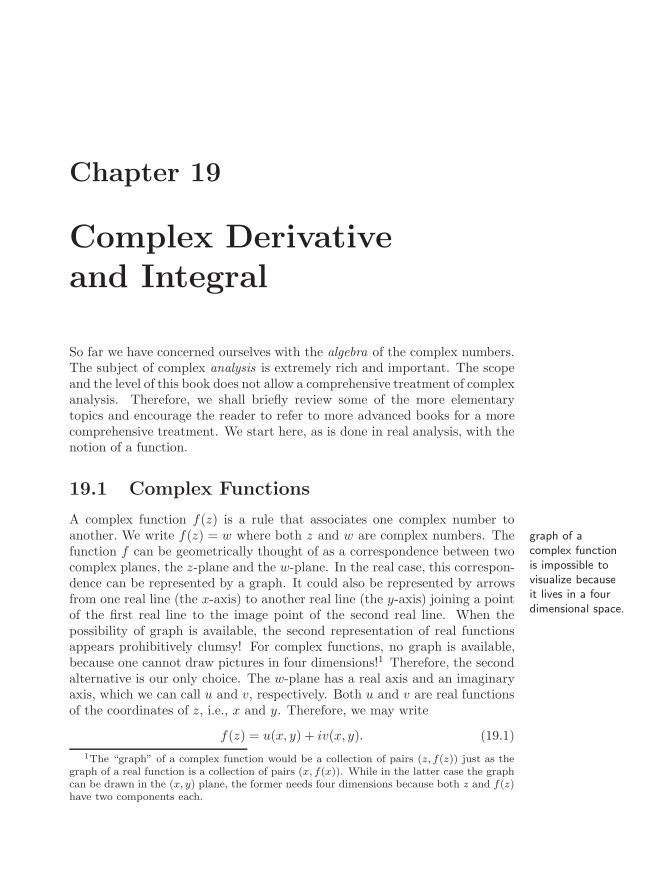
Chapter 19

Complex Derivativeand Integral

So far we have concerned ourselves with the algebra of the complex numbers.The subject of complex analysis is extremely rich and important. The scopeand the level of this book does not allow a comprehensive treatment of complexanalysis. Therefore, we shall briefly review some of the more elementarytopics and encourage the reader to refer to more advanced books for a morecomprehensive treatment. We start here, as is done in real analysis, with thenotion of a function.

19.1 Complex Functions

A complex function f(z) is a rule that associates one complex number toanother. We write f(z) = w where both z and w are complex numbers. The graph of a

complex functionis impossible tovisualize becauseit lives in a fourdimensional space.

function f can be geometrically thought of as a correspondence between twocomplex planes, the z-plane and the w-plane. In the real case, this correspon-dence can be represented by a graph. It could also be represented by arrowsfrom one real line (the x-axis) to another real line (the y-axis) joining a pointof the first real line to the image point of the second real line. When thepossibility of graph is available, the second representation of real functionsappears prohibitively clumsy! For complex functions, no graph is available,because one cannot draw pictures in four dimensions!1 Therefore, the secondalternative is our only choice. The w-plane has a real axis and an imaginaryaxis, which we can call u and v, respectively. Both u and v are real functionsof the coordinates of z, i.e., x and y. Therefore, we may write

f(z) = u(x, y) + iv(x, y). (19.1)1The “graph” of a complex function would be a collection of pairs (z, f(z)) just as the

graph of a real function is a collection of pairs (x, f(x)). While in the latter case the graphcan be drawn in the (x, y) plane, the former needs four dimensions because both z and f(z)have two components each.

498 Complex Derivative and Integral

zw

f

(x, y) (u, v)

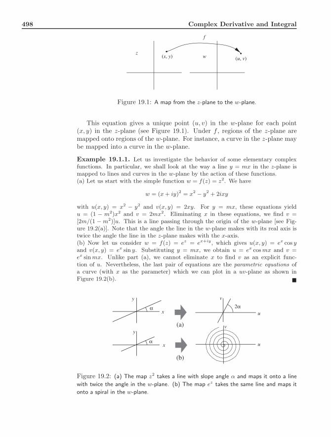
Figure 19.1: A map from the z-plane to the w-plane.

This equation gives a unique point (u, v) in the w-plane for each point(x, y) in the z-plane (see Figure 19.1). Under f , regions of the z-plane aremapped onto regions of the w-plane. For instance, a curve in the z-plane maybe mapped into a curve in the w-plane.

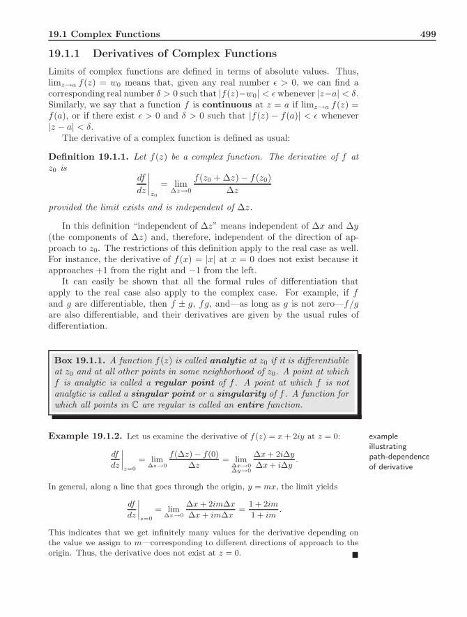
Example 19.1.1. Let us investigate the behavior of some elementary complexfunctions. In particular, we shall look at the way a line y = mx in the z-plane ismapped to lines and curves in the w-plane by the action of these functions.(a) Let us start with the simple function w = f(z) = z2. We have

w = (x + iy)2 = x2 − y2 + 2ixy

with u(x, y) = x2 − y2 and v(x, y) = 2xy. For y = mx, these equations yieldu = (1 − m2)x2 and v = 2mx2. Eliminating x in these equations, we find v =[2m/(1 − m2)]u. This is a line passing through the origin of the w-plane [see Fig-ure 19.2(a)]. Note that the angle the line in the w-plane makes with its real axis istwice the angle the line in the z-plane makes with the x-axis.(b) Now let us consider w = f(z) = ez = ex+iy, which gives u(x, y) = ex cos yand v(x, y) = ex sin y. Substituting y = mx, we obtain u = ex cos mx and v =ex sin mx. Unlike part (a), we cannot eliminate x to find v as an explicit func-tion of u. Nevertheless, the last pair of equations are the parametric equations ofa curve (with x as the parameter) which we can plot in a uv-plane as shown inFigure 19.2(b). !

(a)

α

y

x2α

u

v

(b)

α

y

x u

v

Figure 19.2: (a) The map z2 takes a line with slope angle α and maps it onto a linewith twice the angle in the w-plane. (b) The map ez takes the same line and maps itonto a spiral in the w-plane.

19.1 Complex Functions 499

19.1.1 Derivatives of Complex Functions

Limits of complex functions are defined in terms of absolute values. Thus,limz→a f(z) = w0 means that, given any real number ϵ > 0, we can find acorresponding real number δ > 0 such that |f(z)−w0| < ϵ whenever |z−a| < δ.Similarly, we say that a function f is continuous at z = a if limz→a f(z) =f(a), or if there exist ϵ > 0 and δ > 0 such that |f(z) − f(a)| < ϵ whenever|z − a| < δ.

The derivative of a complex function is defined as usual:

Definition 19.1.1. Let f(z) be a complex function. The derivative of f atz0 is

df

dz

!!!!z0

= lim∆z→0

f(z0 + ∆z) − f(z0)∆z

provided the limit exists and is independent of ∆z.

In this definition “independent of ∆z” means independent of ∆x and ∆y(the components of ∆z) and, therefore, independent of the direction of ap-proach to z0. The restrictions of this definition apply to the real case as well.For instance, the derivative of f(x) = |x| at x = 0 does not exist because itapproaches +1 from the right and −1 from the left.

It can easily be shown that all the formal rules of differentiation thatapply to the real case also apply to the complex case. For example, if fand g are differentiable, then f ± g, fg, and—as long as g is not zero—f/gare also differentiable, and their derivatives are given by the usual rules ofdifferentiation.

Box 19.1.1. A function f(z) is called analytic at z0 if it is differentiableat z0 and at all other points in some neighborhood of z0. A point at whichf is analytic is called a regular point of f . A point at which f is notanalytic is called a singular point or a singularity of f . A function forwhich all points in C are regular is called an entire function.

Example 19.1.2. Let us examine the derivative of f(z) = x + 2iy at z = 0: exampleillustratingpath-dependenceof derivative

dfdz

!!!!z=0

= lim∆z→0

f(∆z) − f(0)∆z

= lim∆x→0∆y→0

∆x + 2i∆y∆x + i∆y

.

In general, along a line that goes through the origin, y = mx, the limit yields

dfdz

!!!!z=0

= lim∆x→0

∆x + 2im∆x∆x + im∆x

=1 + 2im1 + im

.

This indicates that we get infinitely many values for the derivative depending onthe value we assign to m—corresponding to different directions of approach to theorigin. Thus, the derivative does not exist at z = 0. !


A question arises naturally at this point: Under what conditions doesthe limit in the definition of derivative exist? We will find the necessaryand sufficient conditions for the existence of that limit. It is clear from thedefinition that differentiability puts a severe restriction on f(z) because itrequires the limit to be the same for all paths going through z0, the pointat which the derivative is being calculated. Another important point to keepin mind is that differentiability is a local property. To test whether or not afunction f(z) is differentiable at z0, we move away from z0 by a small amount∆z and check the existence of the limit in Definition 19.1.1.

For f(z) = u(x, y) + iv(x, y), Definition 19.1.1 yields

df

dz

!!!!z0

= lim∆x→0∆y→0

"u(x0 + ∆x, y0 + ∆y) − u(x0, y0)

∆x + i∆y

+ iv(x0 + ∆x, y0 + ∆y) − v(x0, y0)

∆x + i∆y

#.

If this limit is to exist for all paths, it must exist for the two particular pathson which ∆y = 0 (parallel to the x-axis) and ∆x = 0 (parallel to the y-axis).For the first path we get

df

dz

!!!!z0

= lim∆x→0

u(x0 + ∆x, y0) − u(x0, y0)∆x

+ i lim∆x→0

v(x0 + ∆x, y0) − v(x0, y0)∆x

=∂u

∂x

!!!!(x0,y0)

+ i∂v

∂x

!!!!(x0,y0)

.

For the second path (∆x = 0), we obtain

df

dz

!!!!z0

= lim∆y→0

u(x0, y0 + ∆y) − u(x0, y0)i∆y

+ i lim∆y→0

v(x0, y0 + ∆y) − v(x0, y0)i∆y

= −i∂u

∂y

!!!!(x0,y0)

+∂v

∂y

!!!!(x0,y0)

.

If f is to be differentiable at z0, the derivatives along the two paths must beequal. Equating the real and imaginary parts of both sides of this equationand ignoring the subscript z0 (x0, y0, or z0 is arbitrary), we obtain

∂u

∂x=

∂v

∂yand

∂u

∂y= −∂v

∂x. (19.2)

These two conditions, which are necessary for the differentiability of f , arecalled the Cauchy–Riemann (C–R) conditions.Cauchy–Riemann

conditions The arguments leading to Equation (19.2) imply that the derivative, if itexists, can be expressed as

df

dz=

∂u

∂x+ i

∂v

∂x=

∂v

∂y− i

∂u

∂y. (19.3)

The C–R conditions assure us that these two equations are equivalent.


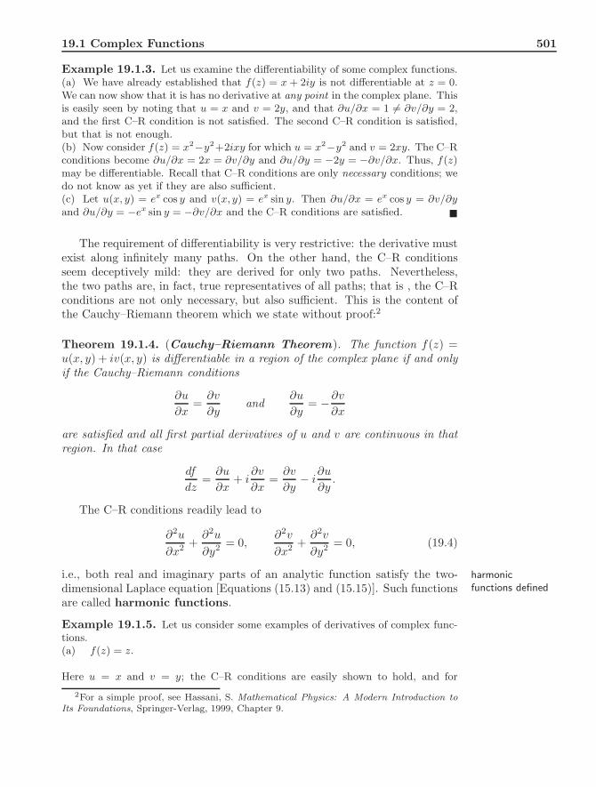
Example 19.1.3. Let us examine the differentiability of some complex functions.(a) We have already established that f(z) = x + 2iy is not differentiable at z = 0.We can now show that it is has no derivative at any point in the complex plane. Thisis easily seen by noting that u = x and v = 2y, and that ∂u/∂x = 1 ̸= ∂v/∂y = 2,and the first C–R condition is not satisfied. The second C–R condition is satisfied,but that is not enough.(b) Now consider f(z) = x2−y2+2ixy for which u = x2−y2 and v = 2xy. The C–Rconditions become ∂u/∂x = 2x = ∂v/∂y and ∂u/∂y = −2y = −∂v/∂x. Thus, f(z)may be differentiable. Recall that C–R conditions are only necessary conditions; wedo not know as yet if they are also sufficient.(c) Let u(x, y) = ex cos y and v(x, y) = ex sin y. Then ∂u/∂x = ex cos y = ∂v/∂yand ∂u/∂y = −ex sin y = −∂v/∂x and the C–R conditions are satisfied. !

The requirement of differentiability is very restrictive: the derivative mustexist along infinitely many paths. On the other hand, the C–R conditionsseem deceptively mild: they are derived for only two paths. Nevertheless,the two paths are, in fact, true representatives of all paths; that is , the C–Rconditions are not only necessary, but also sufficient. This is the content ofthe Cauchy–Riemann theorem which we state without proof:2

Theorem 19.1.4. (Cauchy–Riemann Theorem). The function f(z) =u(x, y) + iv(x, y) is differentiable in a region of the complex plane if and onlyif the Cauchy–Riemann conditions

∂u

∂x=

∂v

∂yand

∂u

∂y= −∂v

∂x

are satisfied and all first partial derivatives of u and v are continuous in thatregion. In that case

df

dz=

∂u

∂x+ i

∂v

∂x=

∂v

∂y− i

∂u

∂y.

The C–R conditions readily lead to

∂2u

∂x2 +∂2u

∂y2 = 0,∂2v

∂x2 +∂2v

∂y2 = 0, (19.4)

i.e., both real and imaginary parts of an analytic function satisfy the two- harmonicfunctions defineddimensional Laplace equation [Equations (15.13) and (15.15)]. Such functions

are called harmonic functions.

Example 19.1.5. Let us consider some examples of derivatives of complex func-tions.(a) f(z) = z.

Here u = x and v = y; the C–R conditions are easily shown to hold, and for

2For a simple proof, see Hassani, S. Mathematical Physics: A Modern Introduction toIts Foundations, Springer-Verlag, 1999, Chapter 9.


any z, we have df/dz = ∂u/∂x + i∂v/∂x = 1. Therefore, the derivative exists at allpoints of the complex plane, i.e., f(z) = z is entire.(b) f(z) = z2.Here u = x2 − y2 and v = 2xy; the C–R conditions hold, and for all points z of thecomplex plane, we have df/dz = ∂u/∂x + i∂v/∂x = 2x + i2y = 2z. Therefore, f(z)is differentiable at all points. So, f(z) = z2 is also entire.(c) f(z) = zn for n ≥ 1.We can use mathematical induction and the fact that the product of two entire

functions is an entire function to show thatddz

(zn) = nzn−1.

(d) f(z) = a0 + a1z + · · · + an−1zn−1 + anzn,where ai are arbitrary constants. That f(z) is entire follows directly from (c) andthe fact that the sum of two entire functions is entire.

(e) f(z) = ez.Here u(x, y) = ex cos y and v(x, y) = ex sin y. Thus, ∂u/∂x = ex cos y = ∂v/∂y and∂u/∂y = −ex sin y = −∂v/∂x and the C–R conditions are satisfied at every point(x, y) of the xy-plane. Furthermore,

dfdz

=∂u∂x

+ i∂v∂x

= ex cos y + iex sin y = ex(cos y + i sin y) = exeiy = ex+iy = ez

and ez is entire as well.(f) f(z) = 1/z.The derivative can be found to be f ′(z) = −1/z2 which does not exist for z = 0.Thus, z = 0 is a singularity of f(z). However, any other point is a regular point of f .

(g) f(z) = 1/ sin z.This gives df/dz = − cos z/ sin2 z. Thus, f has (infinitely many) singular points atz = ±nπ for n = 0, 1, 2, . . . . !

Example 19.1.5 shows that any polynomial in z, as well as the exponentialfunction ez is entire. Therefore, any product and/or sum of polynomials andez will also be entire. We can build other entire functions. For instance,eiz and e−iz are entire functions; therefore, the complex trigonometricfunctions, defined bycomplex

trigonometricfunctions sin z =

eiz − e−iz

2iand cos z =

eiz + e−iz

2(19.5)

are also entire functions. Problem 19.7 shows that sin z and cos z have onlyreal zeros.

The complex hyperbolic functions can be defined similarly:complexhyperbolicfunctions sinh z =

ez − e−z

2and cosh z =

ez + e−z

2. (19.6)

Although the sum and product of entire functions are entire, the ratiois not. For instance, if f(z) and g(z) are polynomials of degrees m and n,respectively, then for n > 0, the ratio f(z)/g(z) is not entire, because at thezeros of g(z)—which always exist—the derivative is not defined.


The functions u(x, y) and v(x, y) of an analytic function have an interestingproperty which the following example investigates.

Example 19.1.6. The family of curves u(x, y) = constant is perpendicular to curves of constantu and v areperpendicular.

the family of curves v(x, y) = constant at each point of the complex plane wheref(z) = u + iv is analytic.

This can easily be seen by looking at the normal to the curves. The normal tothe curve u(x, y) = constant is simply ∇u = ⟨∂u/∂x, ∂u/∂y⟩ (see Theorem 12.3.2).Similarly, the normal to the curve v(x, y) = constant is ∇v = ⟨∂v/∂x, ∂v/∂y⟩.Taking the dot product of these two normals, we obtain

(∇u) · (∇v) =∂u∂x

∂v∂x

+∂u∂y

∂v∂y

=∂u∂x

!−∂u

∂y

"+

∂u∂y

!∂u∂x

"= 0

by the C–R conditions. !

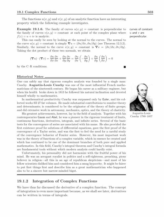
Historical NotesOne can safely say that rigorous complex analysis was founded by a single man:Cauchy. Augustin-Louis Cauchy was one of the most influential French mathe-maticians of the nineteenth century. He began his career as a military engineer, butwhen his health broke down in 1813 he followed his natural inclination and devotedhimself wholly to mathematics.

In mathematical productivity Cauchy was surpassed only by Euler, and his col-lected works fill 27 fat volumes. He made substantial contributions to number theoryand determinants; is considered to be the originator of the theory of finite groups;and did extensive work in astronomy, mechanics, optics, and the theory of elasticity.

Augustin-LouisCauchy 1789–1857

His greatest achievements, however, lay in the field of analysis. Together with hiscontemporaries Gauss and Abel, he was a pioneer in the rigorous treatment of limits,continuous functions, derivatives, integrals, and infinite series. Several of the basictests for the convergence of series are associated with his name. He also provided thefirst existence proof for solutions of differential equations, gave the first proof of theconvergence of a Taylor series, and was the first to feel the need for a careful studyof the convergence behavior of Fourier series. However, his most important workwas in the theory of functions of a complex variable, which in essence he created andwhich has continued to be one of the dominant branches of both pure and appliedmathematics. In this field, Cauchy’s integral theorem and Cauchy’s integral formulaare fundamental tools without which modern analysis could hardly exist.

Unfortunately, his personality did not harmonize with the fruitful power of hismind. He was an arrogant royalist in politics and a self-righteous, preaching, piousbeliever in religion—all this in an age of republican skepticism—and most of hisfellow scientists disliked him and considered him a smug hypocrite. It might be fairerto put first things first and describe him as a great mathematician who happenedalso to be a sincere but narrow-minded bigot.

19.1.2 Integration of Complex Functions

We have thus far discussed the derivative of a complex function. The conceptof integration is even more important because, as we shall see later, derivativescan be written in terms of integrals.


The definite integral of a complex function is naively defined in analogyto that of a real function. However, a crucial difference exists: While in thecomplex integrals

arepath-dependent.

real case, the limits of integration are real numbers and there is only one wayto connect these two limits (along the real line), the limits of integration ofa complex function are points in the complex plane and there are infinitelymany ways to connect these two points. Thus, we speak of a definite integralof a complex function along a path. It follows that complex integrals are, ingeneral, path-dependent.

! α2

α1

f(z) dz = limN→∞∆zi→0

N"

i=1

f(zi)∆zi, (19.7)

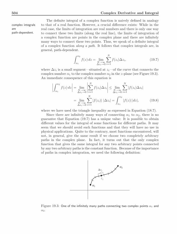
where ∆zi is a small segment—situated at zi—of the curve that connects thecomplex number α1 to the complex number α2 in the z-plane (see Figure 19.3).An immediate consequence of this equation is

####

! α2

α1

f(z) dz

#### = limN→∞∆zi→0

#####

N"

i=1

f(zi)∆zi

##### ≤ limN→∞∆zi→0

N"

i=1

|f(zi)∆zi|

= limN→∞∆zi→0

N"

i=1

|f(zi)| |∆zi| =! α2

α1

|f(z)| |dz|, (19.8)

where we have used the triangle inequality as expressed in Equation (18.7).Since there are infinitely many ways of connecting α1 to α2, there is no

guarantee that Equation (19.7) has a unique value: It is possible to obtaindifferent values for the integral of some functions for different paths. It mayseem that we should avoid such functions and that they will have no use inphysical applications. Quite to the contrary, most functions encountered, willnot, in general, give the same result if we choose two completely arbitrarypaths in the complex plane. In fact, it turns out that the only complexfunction that gives the same integral for any two arbitrary points connectedby any two arbitrary paths is the constant function. Because of the importanceof paths in complex integration, we need the following definition:

α1

α2∆ zi

z i

Figure 19.3: One of the infinitely many paths connecting two complex points α1 andα2.


Box 19.1.2. A contour is a collection of connected smooth arcs. Whenthe beginning point of the first arc coincides with the end point of the lastone, the contour is said to be a simple closed contour (or just closedcontour).

We encountered path-dependent integrals when we tried to evaluate theline integral of a vector field in Chapter 14. The same argument for path-independence can be used to prove (see Problem 19.21)

Theorem 19.1.7. (Cauchy–Goursat Theorem). Let f(z) be analytic ona simple closed contour C and at all points inside C. Then

!

Cf(z) dz = 0

Equivalently," α2

α1f(z) dz is independent of the smooth path connecting α1 and

α2 as long as the path lies entirely in the region of analyticity of f(z).

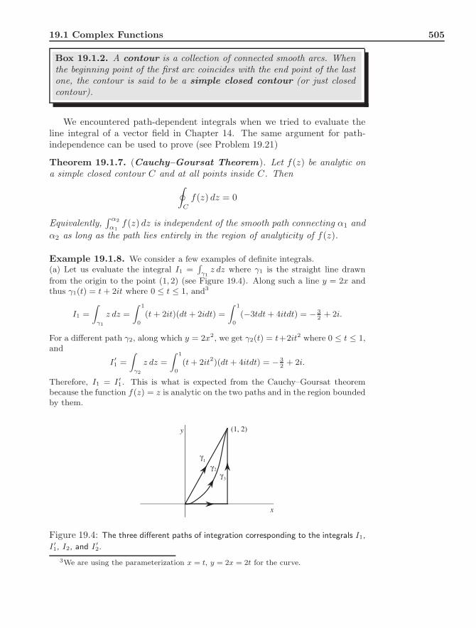
Example 19.1.8. We consider a few examples of definite integrals.(a) Let us evaluate the integral I1 =

"γ1

z dz where γ1 is the straight line drawn

from the origin to the point (1, 2) (see Figure 19.4). Along such a line y = 2x andthus γ1(t) = t + 2it where 0 ≤ t ≤ 1, and3

I1 =

#

γ1

z dz =

# 1

0

(t + 2it)(dt + 2idt) =

# 1

0

(−3tdt + 4itdt) = − 32 + 2i.

For a different path γ2, along which y = 2x2, we get γ2(t) = t+2it2 where 0 ≤ t ≤ 1,and

I ′1 =

#

γ2

z dz =

# 1

0

(t + 2it2)(dt + 4itdt) = − 32 + 2i.

Therefore, I1 = I ′1. This is what is expected from the Cauchy–Goursat theorem

because the function f(z) = z is analytic on the two paths and in the region boundedby them.

γ1

γ 2

γ 3

x

y (1, 2)

Figure 19.4: The three different paths of integration corresponding to the integrals I1,I ′1, I2, and I ′

2.

3We are using the parameterization x = t, y = 2x = 2t for the curve.


(b) Now let us consider I2 =!

γ1z2dz with γ1 as in part (a). Substituting for z in

terms of t, we obtain

I2 =

"

γ1

(t + 2it)2(dt + 2idt) = (1 + 2i)3" 1

0

t2dt = − 113 − 2

3 i.

Next we compare I2 with I ′2 =

!γ3

z2dz where γ3 is as shown in Figure 19.4. Thispath can be described by

γ3(t) =

#t for 0 ≤ t ≤ 1,

1 + i(t − 1) for 1 ≤ t ≤ 3.

Therefore,

I ′2 =

" 1

0

t2dt +

" 3

1

[1 + i(t − 1)]2(idt) = 13 − 4 − 2

3 i = − 113 − 2

3 i,

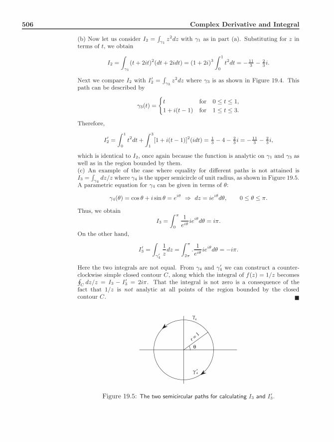
which is identical to I2, once again because the function is analytic on γ1 and γ3 aswell as in the region bounded by them.(c) An example of the case where equality for different paths is not attained isI3 =

!γ4

dz/z where γ4 is the upper semicircle of unit radius, as shown in Figure 19.5.A parametric equation for γ4 can be given in terms of θ:

γ4(θ) = cos θ + i sin θ = eiθ ⇒ dz = ieiθdθ, 0 ≤ θ ≤ π.

Thus, we obtain

I3 =

" π

0

1eiθ

ieiθdθ = iπ.

On the other hand,

I ′3 =

"

γ′4

1zdz =

" π

2π

.1

eiθieiθdθ = −iπ.

Here the two integrals are not equal. From γ4 and γ′4 we can construct a counter-

clockwise simple closed contour C, along which the integral of f(z) = 1/z becomes$C

dz/z = I3 − I ′3 = 2iπ. That the integral is not zero is a consequence of the

fact that 1/z is not analytic at all points of the region bounded by the closedcontour C. !

γ4

′ γ 4

r = 1

θ

Figure 19.5: The two semicircular paths for calculating I3 and I ′3.


C C

ΓL

(a) (b)

Figure 19.6: A contour of integration can be deformed into another contour. Thesecond contour is usually taken to be a circle because of the ease of its correspondingintegration. (a) shows the original contour, and (b) shows the two contours as well asthe (shaded) region between them in which the function is analytic.

The Cauchy–Goursat theorem applies to more complicated regions. Whena region contains points at which f(z) is not analytic, those points can beavoided by redefining the region and the contour (Figure 19.6). Such a pro-cedure requires a convention regarding the direction of “motion” along thecontour. This convention is important enough to be stated separately.

convention forpositive sense ofintegration arounda closed contour

Box 19.1.3. (Convention). When integrating along a closed contour,we agree to traverse the contour in such a way that the region enclosedby the contour lies to our left. An integration that follows this conventionis called integration in the positive sense. Integration performed in theopposite direction acquires a minus sign.

Suppose that we want to evaluate the integral!

C f(z) dz where C is somecontour in the complex plane [see Figure 19.6(a)]. Let Γ be another—usuallysimpler, say a circle—contour which is either entirely inside or entirely out-side C. Figure 19.6 illustrates the case where Γ is entirely inside C. Weassume that Γ is such that f(z) does not have any singularity in the regionbetween C and Γ. By connecting the two contours with a line as shown inFigure 19.6(b), we construct a composite closed contour consisting of C, Γ,and twice the line segment L, once in the positive directions and once inthe negative. Within this composite contour, the function f(z) is analytic.Therefore, by the Cauchy–Goursat theorem, we have

−"

Cf(z) dz +

"

Γf(z) dz +

#

Lf(z) dz −

#

Lf(z) dz = 0.

The negative sign for C is due to the convention above. It follows from thisequation that the integral along C is the same as that along the circle Γ. Thisresult can be interpreted by saying that


Box 19.1.4. We can always deform the contour of an integral in the com-plex plane into a simpler contour, as long as in the process of deformationwe encounter no singularity of the function.

19.1.3 Cauchy Integral Formula

One extremely important consequence of the Cauchy–Goursat theorem, thecenterpiece of complex analysis, is the Cauchy integral formula which we statewithout proof.4

Theorem 19.1.9. Let f(z) be analytic on and within a simple closed contourC integrated in the positive sense. Let z0 be any interior point of C. Then

f(z0) =1

2πi

!

C

f(z)z − z0

dz.

This is called the Cauchy integral formula (CIF).

Example 19.1.10. We can use the CIF to evaluate the following integrals:

I1 =

!

C1

z2 dz(z2 + 3)2(z − i)

, I2 =

!

C2

(z2 − 1) dz

(z − 12 )(z2 − 4)3

,

I3 =

!

C3

ez/2 dz(z − iπ)(z2 − 20)4

,

where C1, C2, and C3 are circles centered at the origin with radii r1 = 32 , r2 = 1,

and r3 = 4, respectively.For I1 we note that f(z) = z2/(z2 +3)2 is analytic within and on C1, and z0 = i

lies in the interior of C1. Thus,

I1 =

!

C1

f(z)dzz − i

= 2πif(i) = 2πii2

(i2 + 3)2= −i

π2

.

Similarly, f(z) = (z2 − 1)/(z2 − 4)3 for I2 is analytic on and within C2, and z0 = 12

is an interior point of C2. Thus, the CIF gives

I2 =

!

C2

f(z)dz

z − 12

= 2πif( 12 ) = 2πi

14 − 1

( 14 − 4)3

=32π1125

i.

For the last integral, f(z) = ez/2/(z2 − 20)4, and the interior point is z0 = iπ:

I3 =

!

C3

f(z)dzz − iπ

= 2πif(iπ) = 2πieiπ/2

(−π2 − 20)4= − 2π

(π2 + 20)4. !

The CIF gives the value of an analytic function at every point inside asimple closed contour when it is given the value of the function only at pointson the contour. It seems as though analytic functions have no freedom withinwhy analytic

functions “remotesense” their valuesat distant points

a contour: They are not free to change inside a region once their value isfixed on the contour enclosing that region. There is an analogous situation in

4For a proof, see Hassani, S. Mathematical Physics: A Modern Introduction to Its Foun-dations, Springer-Verlag, 1999, Chapter 9.


certain areas of physics, for example, electrostatics: The specification of thepotential at the boundaries, such as conductors, automatically determines itat any other point in the region of space bounded by the conductors. This isthe content of the uniqueness theorem (to be discussed later in this book) usedin electrostatic boundary-value problems. However, the electrostatic potentialΦ is bound by another condition, Laplace’s equation; and the combination ofLaplace’s equation and the boundary conditions furnishes the uniqueness of Φ.

It seems, on the other hand, as though the mere specification of an analyticfunction on a contour, without any other condition, is sufficient to determinethe function’s value at all points enclosed within that contour. This is notthe case. An analytic function, by its very definition, satisfies another re-strictive condition: Its real and imaginary parts separately satisfy Laplace’sequation in two dimensions! [see Equation (19.4)]. Thus, it should come asno surprise that the value of an analytic function at a boundary (contour)determines the function at all points inside the boundary.

19.1.4 Derivatives as Integrals

The CIF is a very powerful tool for working with analytic functions. Oneof the applications of this formula is in evaluating the derivatives of suchfunctions. It is convenient to change the dummy integration variable to ξ andwrite the CIF as

f(z) =1

2πi

!

C

f(ξ) dξ

ξ − z, (19.9)

where C is a simple closed contour in the ξ-plane and z is a point within C.By carrying the derivative inside the integral, we get

df

dz=

12πi

d

dz

!

C

f(ξ) dξ

ξ − z=

12πi

!

C

d

dz

"f(ξ) dξ

ξ − z

#=

12πi

!

C

f(ξ) dξ

(ξ − z)2.

By repeated differentiation, we can generalize this formula to the nth deriva-tive, and obtain

Theorem 19.1.11. The derivatives of all orders of an analytic function f(z)exist in the domain of analyticity of the function and are themselves analyticin that domain. The nth derivative of f(z) is given by

f (n)(z) =dnf

dzn =n!2πi

!

C

f(ξ) dξ

(ξ − z)n+1. (19.10)

Example 19.1.12. Let us apply Equation (19.10) directly to some simple func-tions. In all cases, we will assume that the contour is a circle of radius r centeredat z.(a) Let f(z) = K, a constant. Then, for n = 1 we have

dfdz

=1

2πi

!

C

K dξ(ξ − z)2

.


Since ξ is always on the circle C centered at z, ξ − z = reiθ and dξ = rieiθdθ. Sowe have

dfdz

=1

2πi

! 2π

0

Kireiθdθ(reiθ)2

=K

2πr

! 2π

0

e−iθdθ = 0.

That is, the derivative of a constant is zero.(b) Given f(z) = z, its first derivative will be

dfdz

=1

2πi

"

C

ξ dξ(ξ − z)2

=1

2πi

! 2π

0

(z + reiθ)ireiθdθ(reiθ)2

=12π

#zr

! 2π

0

e−iθdθ +

! 2π

0

dθ

$=

12π

(0 + 2π) = 1.

(c) Given f(z) = z2, for the first derivative Equation (19.10) yields

dfdz

=1

2πi

"

C

ξ2 dξ(ξ − z)2

=1

2πi

! 2π

0

(z + reiθ)2ireiθdθ(reiθ)2

=12π

! 2π

0

%z2 + (reiθ)2 + 2zreiθ

&(reiθ)−1dθ

=12π

#z2

r

! 2π

0

e−iθdθ + r

! 2π

0

eiθdθ + 2z

! 2π

0

dθ

$= 2z.

It can be shown that, in general, (d/dz)zm = mzm−1. The proof is left as Problem19.24. !

The CIF is a central formula in complex analysis. However, due to spacelimitations, we cannot explore its full capability here. Nevertheless, one of itsapplications is worth discussing at this point. Suppose that f is a boundedentire function and consider

df

dz=

12πi

"

C

f(ξ) dξ

(ξ − z)2.

Since f is analytic everywhere in the complex plane, the closed contour C canbe chosen to be a very large circle of radius R with center at z. Taking theabsolute value of both sides yields

''''df

dz

'''' =12π

''''! 2π

0

f(z + Reiθ)(Reiθ)2

iReiθdθ

''''

≤ 12π

! 2π

0

|f(z + Reiθ)|R

dθ ≤ 12π

! 2π

0

M

Rdθ =

M

R,

where we used Equation (19.8) and |eiθ| = 1. M is the maximum of thefunction in the complex plane.5 Now as R → ∞, the derivative goes to zero.The only function whose derivative is zero is the constant function. Thus

Box 19.1.5. A bounded entire function is necessarily a constant.

5M exists because f is assumed to be bounded.

19.2 Problems 511

There are many interesting and nontrivial real functions that are bounded andhave derivatives (of all orders) on the entire real line. For instance, e−x2

is such any nontrivialfunction is eitherunbounded or notentire.

a function. No such freedom exists for complex analytic functions accordingto Box 19.1.5! Any nontrivial analytic function is either not bounded (goesto infinity somewhere on the complex plane) or not entire [it is not analyticat some point(s) of the complex plane].

A consequence of Proposition 19.1.5 is the fundamental theorem ofalgebra which states that any polynomial of degree n ≥ 1 has n roots (some fundamental

theorem of algebraproved

of which may be repeated). In other words, the polynomial

p(x) = a0 + a1x + · · · + anxn for n ≥ 1

can be factored completely as p(x) = c(x − z1)(x − z2) . . . (x − zn) where c isa constant and the zi are, in general, complex numbers.

To see how Proposition 19.1.5 implies the fundamental theorem of algebra,we let f(z) = 1/p(z) and assume the contrary, i.e., that p(z) is never zero forany (finite) z. Then f(z) is bounded and analytic for all z, and Proposition19.1.5 says that f(z) is a constant. This is obviously wrong. Thus, there mustbe at least one z, say z = z1, for which p(z) is zero. So, we can factor out(z − z1) from p(z) and write p(z) = (z − z1)q(z) where q(z) is of degree n− 1.Applying the above argument to q(z), we have p(z) = (z − z1)(z − z2)r(z)where r(z) is of degree n− 2. Continuing in this way, we can factor p(z) intolinear factors. The last polynomial will be a constant (a polynomial of degreezero) which we have denoted as c.

19.2 Problems

19.1. Show that f(z) = z2 maps a line that makes an angle α with thereal axis of the z-plane onto a line in the w-plane which makes an angle2α with the real axis of the w-plane. Hint: Use the trigonometric identitytan 2α = 2 tanα/(1 − tan2 α).

19.2. Show that the function w = 1/z maps the straight line y = 12 in the

z-plane onto a circle in the w-plane.

19.3. (a) Using the chain rule, find ∂f/∂z∗ and ∂f/∂z in terms of partialderivatives with respect to x and y.(b) Evaluate ∂f/∂z∗ and ∂f/∂z assuming that the C–R conditions hold.

19.4. (a) Show that, when z is represented by polar coordinates, the C–Rconditions on a function f(z) are

∂U

∂r=

1r

∂V

∂θ,

∂U

∂θ= −r

∂V

∂r,

where U and V are the real and imaginary parts of f(z) written in polarcoordinates.


(b) Show that the derivative of f can be written as

df

dz= e−iθ

!∂U

∂r+ i

∂V

∂r

".

Hint: Start with the C–R conditions in Cartesian coordinates and apply thechain rule to them using x = r cos θ and y = r sin θ.

19.5. Prove the following identities for differentiation by finding the realand imaginary parts of the function—u(x, y) and v(x, y)—and differentiat-ing them:

(a)d

dz(f + g) =

df

dz+

dg

dz. (b)

d

dz(fg) =

df

dzg + f

dg

dz.

(c)d

dz

!f

g

"=

f ′(z)g(z)− g′(z)f(z)[g(z)]2

, where g(z) ̸= 0.

19.6. Show that d/dz(ln z) = 1/z. Hint: Find u(x, y) and v(x, y) for ln zusing the exponential representation of z, then differentiate them.

19.7. Show that sin z and cos z have only real roots. Hint: Use definition ofsine and cosine in terms of exponentials.

19.8. Use mathematical induction and the product rule for differentiation to

show thatd

dz(zn) = nzn−1.

19.9. Use Equations (19.5) and (19.6), to establish the following identities:

(a) Re(sin z) = sin x cosh y, Im(sin z) = cosx sinh y.

(b) Re(cos z) = cosx cosh y, Im(cos z) = − sin x sinh y.

(c) Re(sinh z) = sinhx cos y, Im(sinh z) = cosh x sin y.

(d) Re(cosh z) = coshx cos y, Im(cosh z) = sinhx sin y.

(e) | sin z|2 = sin2 x + sinh2 y, | cos z|2 = cos2 x + sinh2 y.

(f) | sinh z|2 = sinh2 x + sin2 y, | cosh z|2 = sinh2 x + cos2 y.

19.10. Find all the zeros of sinh z and cosh z.

19.11. Verify the following trigonometric identities:

(a) cos2 z + sin2 z = 1.

(b) cos(z1 + z2) = cos z1 cos z2 − sin z1 sin z2.

(c) sin(z1 + z2) = sin z1 cos z2 + cos z1 sin z2.

(d) sin#π

2− z

$= cos z, cos

#π

2− z

$= sin z.

(e) cos 2z = cos2 z − sin2 z, sin 2z = 2 sin z cos z.

(f) tan(z1 + z2) =tan z1 + tan z2

1 − tan z1 tan z2.

19.2 Problems 513

19.12. Verify the following hyperbolic identities:

(a) cosh2 z − sinh2 z = 1.

(b) cosh(z1 + z2) = cosh z1 cosh z2 + sinh z1 sinh z2.

(c) sinh(z1 + z2) = sin z1 cosh z2 + cosh z1 sinh z2.

(d) cosh 2z = cosh2 z + sinh2 z, sinh 2z = 2 sinh z cosh z.

(e) tanh(z1 + z2) =tanh z1 + tanh z2

1 + tanh z1 tanh z2.

19.13. Show that

(a) tanh!z

2

"=

sinh x + i sin y

cosh x + cos y. (b) coth

!z

2

"=

sinh x − i sin y

coshx − cos y.

19.14. Prove the following identities:

(a) cos−1 z = −i ln(z ±#

z2 − 1). (b) sin−1 z = −i ln[iz ±#

1 − z2)].

(c) tan−1 z =12i

ln$

i − z

i + z

%. (d) cosh−1 z = ln(z ±

#z2 − 1).

(e) sinh−1 z = ln(z ±#

z2 + 1). (f) tanh−1 z = 12 ln

$1 + z

1 − z

%.

19.15. Prove that exp(z∗) is not analytic anywhere.

19.16. Show that eiz = cos z + i sin z for any z.

19.17. Show that both the real and imaginary parts of an analytic functionare harmonic.

19.18. Show that each of the following functions—call each one u(x, y)—is harmonic, and find the function’s harmonic partner, v(x, y), such thatu(x, y) + iv(x, y) is analytic. Hint: Use C–R conditions.

(a)x3 − 3xy2. (b) ex cos y. (c)x

x2 + y2where x2 + y2 ̸= 0.

(d) e−2y cos 2x. (e) ey2−x2cos 2xy.

(f) ex(x cos y − y sin y) + 2 sinh y sin x + x3 − 3xy2 + y.

19.19. Describe the curve defined by each of the following equations:

(a) z = 1 − it, 0 ≤ t ≤ 2. (b) z = t + it2, −∞ < t < ∞.

(c) z = a(cos t + i sin t)π

2≤ t ≤ 3π

2. (d) z = t +

i

t−∞ < t < 0.

19.20. Let f(z) = w = u+ iv. Suppose that∂2Φ∂x2

+∂2Φ∂y2

= 0. Show that if f

is analytic, then∂2Φ∂u2

+∂2Φ∂v2

= 0. That is, analytic functions map harmonicfunctions in the z-plane to harmonic functions in the w-plane.


19.21. (a) Show that!

f(z) dz can be written as"

A · dr + i

"B · dr,

where A = ⟨u,−v, 0⟩, B = ⟨v, u, 0⟩, and dr = ⟨dx, dy, 0⟩.(b) Show that both A and B have vanishing curls when f is analytic.(c) Now use the Stokes’ theorem to prove the Cauchy–Goursat theorem.

19.22. Find the value of the integral!

C [(z + 2)/z] dz, where C is: (a) thesemicircle z = 2eiθ, for 0 ≤ θ ≤ π; (b) the semicircle z = 2eiθ, for π ≤ θ ≤ 2π;and (c) the circle z = 2eiθ, for −π ≤ θ ≤ π.

19.23. Evaluate the integral!

γ dz/(z − 1− i) where γ is: (a) the line joiningz1 = 2i and z2 = 3; and (b) the path from z1 to the origin and from there toz2.

19.24. Use Equation (19.10) to show thatd

dz(zm) = mzm−1. Hint: Use the

binomial theorem.

19.25. Let C be the boundary of a square whose sides lie along the linesx = ±3 and y = ±3. For the positive sense of integration, evaluate each ofthe following integrals by using CIF or the derivative formula (19.10):

(a)#

C

e−z

z − iπ/2dz. (b)

#

C

ez

z(z2 + 10)dz. (c)

#

C

cos z

(z − π4 )(z2 − 10)

dz.

(d)#

C

sinh z

z4dz. (e)

#

C

cosh z

z4dz. (f)

#

C

cos z

z3dz.

(g)#

C

cos z

(z − iπ/2)2dz. (h)

#

C

ez

(z − iπ)2dz. (i)

#

C

cos z

z + iπdz.

(j)#

C

ez

z2 − 5z + 4dz. (k)

#

C

sinh z

(z − iπ/2)2dz. (l)

#

C

cosh z

(z − π/2)2dz.

(m)#

C

z2

(z − 2)(z2 − 10)dz.

Complex Derivative and Integral

Documents

Transcript of Complex Derivative and Integral