Fundamentals of Bicomplex Pseudoanalytic Function Theory: Cauchy Integral Formulas, Negative Formal...
31
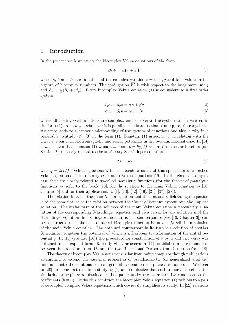
arXiv:1205.4654v1 [math.CV] 21 May 2012 Fundamentals of bicomplex pseudoanalytic function theory: Cauchy integral formulas, negative formal powers and Schr¨odinger equations withcomplex coefficients Hugo M. Campos and Vladislav V. Kravchenko Departamento de Matem´ aticas, CINVESTAV del IPN, Unidad Queretaro, Libramiento Norponiente No. 2000, Fracc. Real de Juriquilla, Queretaro, Qro. C.P. 76230 MEXICO e-mail: [email protected]; [email protected] * May 22, 2012 Abstract The study of the Dirac system and second-order elliptic equations with complex- valued coefficients on the plane naturally leads to bicomplex Vekua-type equations [8], [14], [6]. To the difference of complex pseudoanalytic (or generalized analytic) functions [3], [25] the theory of bicomplex pseudoanalytic functions has not been developed. Such basic facts as, e.g., the similarity principle or the Liouville theorem in general are no longer available due to the presence of zero divisors in the algebra of bicomplex numbers. In the present work we develop a theory of bicomplex pseudoanalytic formal powers analogous to the developed by L. Bers [3] and especially that of negative formal powers. Combining the approaches of L. Bers and I. N. Vekua with some additional ideas we obtain the Cauchy integral formula in the bicomplex setting. In the classical complex situation this formula was obtained under the assumption that the involved Cauchy kernel is global, a very restrictive condition taking into account possible practical applications, especially when the equation itself is not defined on the whole plane. We show that the Cauchy integral formula remains valid with the Cauchy kernel from a wider class called here the reproducing Cauchy kernels. We give a complete characterization of this class. To our best knowledge these results are new even for complex Vekua equations. We establish that reproducing Cauchy kernels can be used to obtain a full set of negative formal powers for the corresponding bicomplex Vekua equation and present an algorithm which allows one their construction. Bicomplex Vekua equations of a special form called main Vekua equations are closely related to stationary Schr¨odinger equations with complex-valued potentials. We use this relation to establish useful connections between the reproducing Cauchy kernels and the fundamental solutions for the Schr¨odinger operators which allow one to construct the Cauchy kernel when the fundamental solution is known and vice versa. Moreover, using these results we construct the fundamental solutions for the Darboux transformed Schr¨odingeroperators. * Research was supported by CONACYT, Mexico. Hugo Campos additionally acknowledges the support by FCT, Portugal. 1
-
Upload
independent -
Category
Documents
-
view
1 -
download
0
Transcript of Fundamentals of Bicomplex Pseudoanalytic Function Theory: Cauchy Integral Formulas, Negative Formal...
arX
iv:1
205.
4654
v1 [
mat
h.C
V]
21
May
201
2
Fundamentals of bicomplex pseudoanalytic function theory:
Cauchy integral formulas, negative formal powers and
Schrodinger equations with complex coefficients
Hugo M. Campos and Vladislav V. Kravchenko
Departamento de Matematicas, CINVESTAV del IPN, Unidad Queretaro,
Libramiento Norponiente No. 2000, Fracc. Real de Juriquilla, Queretaro,
Qro. C.P. 76230 MEXICO e-mail: [email protected];
May 22, 2012
Abstract
The study of the Dirac system and second-order elliptic equations with complex-valued coefficients on the plane naturally leads to bicomplex Vekua-type equations [8],[14], [6]. To the difference of complex pseudoanalytic (or generalized analytic) functions[3], [25] the theory of bicomplex pseudoanalytic functions has not been developed. Suchbasic facts as, e.g., the similarity principle or the Liouville theorem in general are nolonger available due to the presence of zero divisors in the algebra of bicomplex numbers.
In the present work we develop a theory of bicomplex pseudoanalytic formal powersanalogous to the developed by L. Bers [3] and especially that of negative formal powers.Combining the approaches of L. Bers and I. N. Vekua with some additional ideas weobtain the Cauchy integral formula in the bicomplex setting. In the classical complexsituation this formula was obtained under the assumption that the involved Cauchy kernelis global, a very restrictive condition taking into account possible practical applications,especially when the equation itself is not defined on the whole plane. We show that theCauchy integral formula remains valid with the Cauchy kernel from a wider class calledhere the reproducing Cauchy kernels. We give a complete characterization of this class.To our best knowledge these results are new even for complex Vekua equations. Weestablish that reproducing Cauchy kernels can be used to obtain a full set of negativeformal powers for the corresponding bicomplex Vekua equation and present an algorithmwhich allows one their construction.
Bicomplex Vekua equations of a special form called main Vekua equations are closelyrelated to stationary Schrodinger equations with complex-valued potentials. We use thisrelation to establish useful connections between the reproducing Cauchy kernels andthe fundamental solutions for the Schrodinger operators which allow one to constructthe Cauchy kernel when the fundamental solution is known and vice versa. Moreover,using these results we construct the fundamental solutions for the Darboux transformedSchrodinger operators.
∗Research was supported by CONACYT, Mexico. Hugo Campos additionally acknowledges the support
by FCT, Portugal.
1
1 Introduction
In the present work we study the bicomplex Vekua equations of the form
∂zW = aW + bW (1)
where a, b and W are functions of the complex variable z = x + jy and take values in thealgebra of bicomplex numbers. The conjugation W is with respect to the imaginary unit jand ∂z = 1
2 (∂x + j∂y). Every bicomplex Vekua equation (1) is equivalent to a first ordersystem
∂xu− ∂yv = αu+ βv (2)
∂xv + ∂yu = γu+ δv (3)
where all the involved functions are complex, and vice versa, the system can be written inthe form (1). As always, whenever it is possible, the introduction of an appropriate algebraicstructure leads to a deeper understanding of the system of equations and this is why it ispreferable to study (2), (3) in the form (1). Equation (1) arised in [8] in relation with theDirac system with electromagnetic and scalar potentials in the two-dimensional case. In [14]it was shown that equation (1) when a ≡ 0 and b = ∂zf/f where f is a scalar function (seeSection 2) is closely related to the stationary Schrodinger equation
∆u = qu (4)
with q = ∆f/f . Vekua equations with coefficients a and b of this special form are calledVekua equations of the main type or main Vekua equations [16]. In the classical complexcase they are closely related to so-called p-analytic functions (for the theory of p-analyticfunctions we refer to the book [20], for the relation to the main Vekua equation to [16,Chapter 5] and for their applications to [1], [10], [12], [16], [21], [27], [28]).
The relation between the main Vekua equation and the stationary Schrodinger equationis of the same nature as the relation between the Cauchy-Riemann system and the Laplaceequation. The scalar part of the solution of the main Vekua equation is necessarily a so-lution of the corresponding Schrodinger equation and vice versa, for any solution u of theSchrodinger equation its “conjugate metaharmonic” counterpart v (see [16, Chapter 3]) canbe constructed such that the obtained bicomplex function W = u + jv will be a solutionof the main Vekua equation. The obtained counterpart in its turn is a solution of anotherSchrodinger equation the potential of which is a Darboux transformation of the initial po-tential q. In [13] (see also [16]) the procedure for construction of v by u and vice versa wasobtained in the explicit form. Recently Sh. Garuchava in [11] established a correspondencebetween the procedure from [13] and the two-dimensional Darboux transformation from [19].
The theory of bicomplex Vekua equations is far from being complete though publicationsattempting to extend the essential properties of pseudoanalytic (or generalized analytic)functions onto the solutions of more general systems on the plane are numerous. We referto [26] for some first results in studying (1) and emphasize that such important facts as thesimilarity principle were obtained in that paper under the overrestrictive condition on thecoefficients (b ≡ 0). Under this condition the bicomplex Vekua equation (1) reduces to a pairof decoupled complex Vekua equations which obviously simplifies its study. In [22] relations
2

between classes of bicomplex Vekua equations and complexified Schrodinger equations werestudied. In the recent work [2] several results on bicomplex pseudoanalytic functions fromthe point of view of Bauer-Peschl differential operators can be found.
The main difficulty in studying the bicomplex Vekua equation comes from the existenceof zero divisors in the algebra of bicomplex numbers. For example, when the solution Wof (1) does not have zero divisors (the values of the function do not coincide with a zerodivisor at any point z of the domain of interest) for such W we prove a similarity principle(Theorem 14 below). Unfortunately in general this fact is unavailable which forces one tolook for alternative ideas for developing the corresponding pseudoanalytic function theory.
In [6], [8], [14], [16] it was noticed that several constructive results from Bers’ theoryremain valid in the bicomplex case. For example, if a generating sequence correspondingto the bicomplex Vekua equation (1) is known, the construction of corresponding positiveformal powers can be performed by means of Bers’ algorithm based on the concept of the(F,G)-integration. However to the difference from the complex pseudoanalytic functiontheory it is not clear how to prove the expansion and Runge theorems in the bicomplex case,the results ensuring the completeness of the formal powers in the space of all solutions ofthe Vekua equation. Moreover, these results in the classical complex case were obtained forglobal formal powers only (see the definition in Subsection 3.3) meanwhile the only systemof formal powers whose explicit form is known corresponds to the case of analytic functions,(z − z0)
n∞0 . Recently for a wide class of main bicomplex Vekua equations the expansionand the Runge theorems were obtained in [6], [7] using the approach based on so-calledtransmutation (or transformation) operators. It is important to emphasize that in [6] and[7] the results concerning the completeness of systems of local formal powers were obtainedwhich opened the way to apply them in practical solution of boundary value and eigenvalueproblems for second-order elliptic equations with variable coefficients (see [5] and [9]).
The main subject of the present work is the study of negative formal powers for thebicomplex Vekua equation and their applications. Based on the results on the Cauchy kernelswe obtain Cauchy integral formulas for bicomplex pseudoanalytic functions. In the classicaltheory of complex pseudoanalytic functions in fact there are two types of Cauchy integralformulas. One is based on Cauchy kernels for an adjoint Vekua equation and the otherinvolves the Cauchy kernels for the initial Vekua equation (here we call these two Cauchyintegral formulas the first and the second respectively). We obtain a relation between bothCauchy kernels and prove both kinds of Cauchy integral formulas. It is important to mentionthat the Cauchy kernels involved in the obtained Cauchy integral formulas are not required tobe global but instead belong to a much more general class which we call reproducing Cauchykernels. We give a complete characterization of this class. To our best knowledge theseresults are new even for complex Vekua equations. We establish that reproducing Cauchykernels can be used to obtain a full set of negative formal powers for the correspondingbicomplex Vekua equation and present an algorithm which allows one their construction.
Bicomplex Vekua equations of a special form called main Vekua equations are closelyrelated to stationary Schrodinger equations with complex-valued potentials. We use thisrelation to establish direct connections between the reproducing Cauchy kernels and thefundamental solutions for the Schrodinger operators which allow one to construct the Cauchykernel when the fundamental solution is known and vice versa. Moreover, using these resultswe construct the fundamental solutions for the Darboux transformed Schrodinger operators.
3

These results are also new in the context of the classical complex Vekua equations and amongother applications allow one to obtain in a closed form a reproducing Cauchy kernel and aset of negative formal powers for an important class of main Vekua equations.
The layout of the paper is as follows. In Section 2 we introduce the necessary formal-ism concerning the bicomplex numbers. Some of the facts presented here can be found inseveral sources, e.g., [17], [23], [24]. Nevertheless we needed to introduce a special thoughquite natural norm and hence prove several related properties which probably are first pub-lished. In Section 3 we introduce the necessary definitions from pseudoanalytic functiontheory, prove several results concerning bicomplex pseudoanalytic functions, like the men-tioned above similarity principle (for functions without zero divisors). By analogy with thecomplex case we define formal powers and obtain their basic properties. We introduce themain Vekua equation in relation with the stationary Schrodinger equation and obtain someauxiliary results for its solutions. In Section 4 the Cauchy integral formulas for bicomplexpseudoanalytic functions are obtained and the characterization of the reproducing Cauchykernels is given. In Section 5 we establish an important relation between the negative formalpowers corresponding to different bicomplex Vekua equations which in fact leads to an algo-rithm for constructing the negative formal powers. We give several applications of this resultin Section 6 using a valuable observation that for the main Vekua equation the adjoint andthe successor coincide. This leads to the possibility to construct a reproducing Cauchy kernelfor the Vekua equation from a known fundamental solution for a related Schrodinger equa-tion and vice versa and also gives a method for constructing the fundamental solutions for achain of Darboux transformed Schrodinger operators. Finally, several examples of explicitlycalculated kernels and fundamental solutions are presented.
2 Bicomplex numbers
Together with the imaginary unit i we consider another imaginary unit j, such that
j2 = i2 = −1 and i j = j i. (5)
We have then two copies of the field of complex numbers, Ci := a+ ib, a, b ⊂ R andCj := a+ jb, a, b ⊂ R. The expressions of the form W = u+ jv where u, v ⊂ Ci arecalled bicomplex numbers. The conjugation with respect to j we denote as W = u− jv. Thecomponents u and v will be called the scalar and the vector part of W respectively. We willuse the notation u = ScW and v = VecW .
The set of all bicomplex numbers with a natural operation of addition and with themultiplication defined by the laws (5) represents a commutative ring with a unit. We denoteit by B. An element W ∈ B is invertible if and only if WW 6= 0 and the inverse element is
defined by the equality W−1 =W
WW.
Let R(B) be the set formed by the invertible elements of B and σ(B) denote the gener-alized zeros of B (zero divisors), that is
σ(B) =W ∈ B: W 6= 0 and WW = 0
.
It is convenient to introduce the pair of idempotents P+ = 12 (1+ ij) and P− = 1
2 (1− ij)
((P±)2= P±). As it can be verified directly, P± ∈ σ(B) and P+ + P− = 1.
4
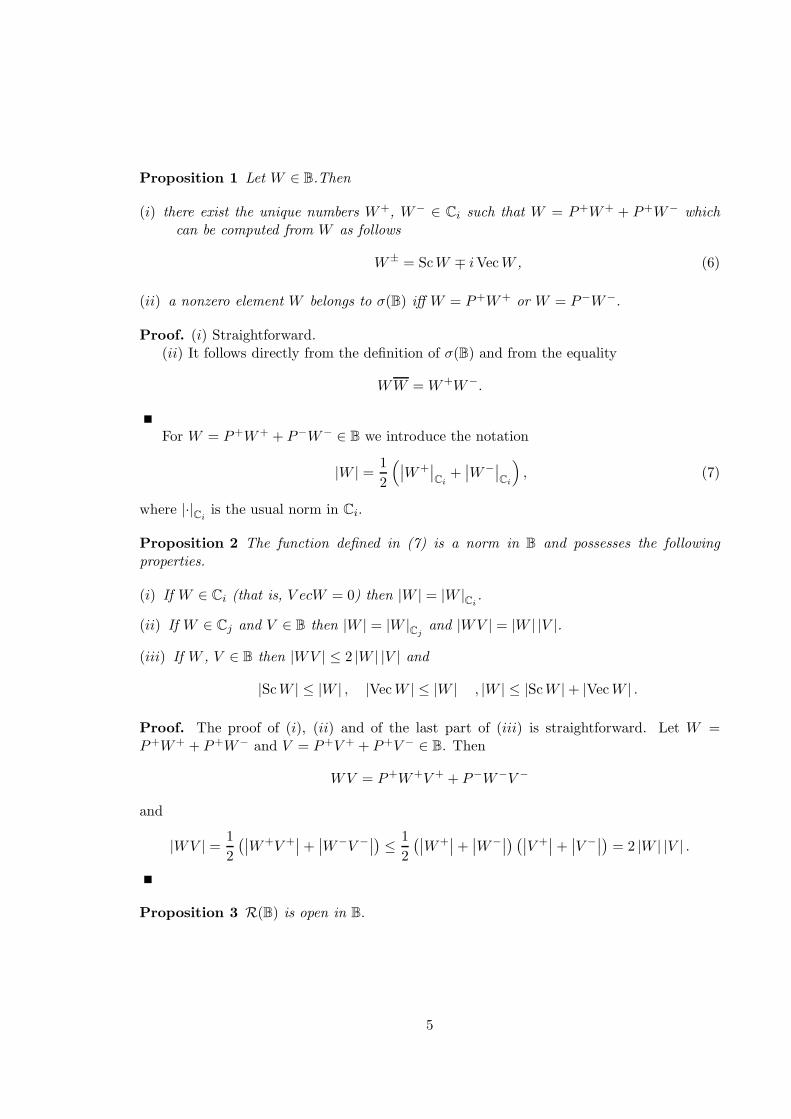
Proposition 1 Let W ∈ B.Then
(i) there exist the unique numbers W+, W− ∈ Ci such that W = P+W+ + P+W− whichcan be computed from W as follows
W± = ScW ∓ iVecW , (6)
(ii) a nonzero element W belongs to σ(B) iff W = P+W+ or W = P−W−.
Proof. (i) Straightforward.(ii) It follows directly from the definition of σ(B) and from the equality
WW =W+W−.
For W = P+W+ + P−W− ∈ B we introduce the notation
|W | =1
2
(∣∣W+∣∣Ci
+∣∣W−
∣∣Ci
), (7)
where |·|Ci
is the usual norm in Ci.
Proposition 2 The function defined in (7) is a norm in B and possesses the followingproperties.
(i) If W ∈ Ci (that is, V ecW = 0) then |W | = |W |Ci.
(ii) If W ∈ Cj and V ∈ B then |W | = |W |Cj
and |WV | = |W | |V |.
(iii) If W , V ∈ B then |WV | ≤ 2 |W | |V | and
|ScW | ≤ |W | , |VecW | ≤ |W | , |W | ≤ |ScW |+ |VecW | .
Proof. The proof of (i), (ii) and of the last part of (iii) is straightforward. Let W =P+W+ + P+W− and V = P+V + + P+V − ∈ B. Then
WV = P+W+V + + P−W−V −
and
|WV | =1
2
(∣∣W+V +∣∣+
∣∣W−V −∣∣) ≤ 1
2
(∣∣W+∣∣+
∣∣W−∣∣) (∣∣V +
∣∣+∣∣V −
∣∣) = 2 |W | |V | .
Proposition 3 R(B) is open in B.
5
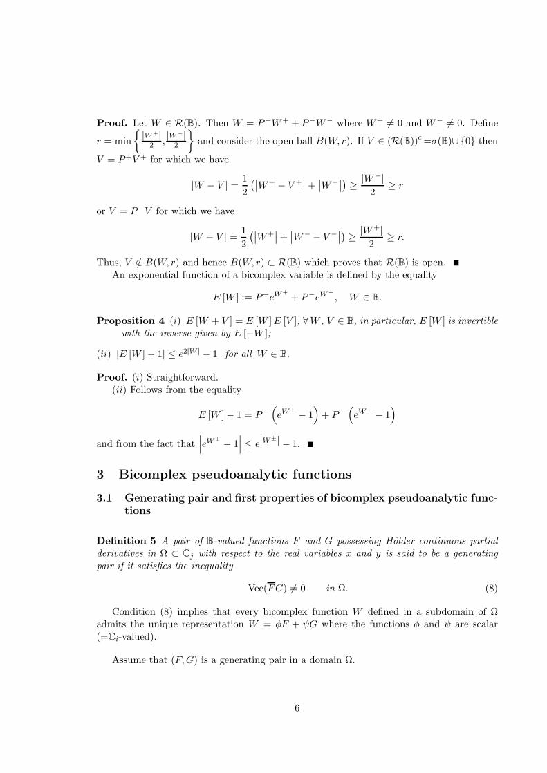
Proof. Let W ∈ R(B). Then W = P+W+ + P−W− where W+ 6= 0 and W− 6= 0. Define
r = min
|W+|
2 ,|W−|
2
and consider the open ball B(W, r). If V ∈ (R(B))c=σ(B)∪0 then
V = P+V + for which we have
|W − V | =1
2
(∣∣W+ − V +∣∣+
∣∣W−∣∣) ≥ |W−|
2≥ r
or V = P−V for which we have
|W − V | =1
2
(∣∣W+∣∣+
∣∣W− − V −∣∣) ≥ |W+|
2≥ r.
Thus, V /∈ B(W, r) and hence B(W, r) ⊂ R(B) which proves that R(B) is open.An exponential function of a bicomplex variable is defined by the equality
E [W ] := P+eW++ P−eW
−
, W ∈ B.
Proposition 4 (i) E [W + V ] = E [W ]E [V ], ∀W , V ∈ B, in particular, E [W ] is invertiblewith the inverse given by E [−W ];
(ii) |E [W ]− 1| ≤ e2|W | − 1 for all W ∈ B.
Proof. (i) Straightforward.(ii) Follows from the equality
E [W ]− 1 = P+(eW
+− 1
)+ P−
(eW
−
− 1)
and from the fact that∣∣∣eW±
− 1∣∣∣ ≤ e|W
±| − 1.
3 Bicomplex pseudoanalytic functions
3.1 Generating pair and first properties of bicomplex pseudoanalytic func-tions
Definition 5 A pair of B-valued functions F and G possessing Holder continuous partialderivatives in Ω ⊂ Cj with respect to the real variables x and y is said to be a generatingpair if it satisfies the inequality
Vec(FG) 6= 0 in Ω. (8)
Condition (8) implies that every bicomplex function W defined in a subdomain of Ωadmits the unique representation W = φF + ψG where the functions φ and ψ are scalar(=Ci-valued).
Assume that (F,G) is a generating pair in a domain Ω.
6
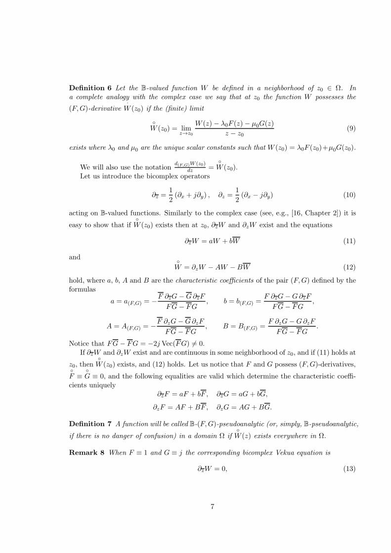
Definition 6 Let the B-valued function W be defined in a neighborhood of z0 ∈ Ω. Ina complete analogy with the complex case we say that at z0 the function W possesses the
(F,G)-derivative·W (z0) if the (finite) limit
W (z0) = lim
z→z0
W (z)− λ0F (z)− µ0G(z)
z − z0(9)
exists where λ0 and µ0 are the unique scalar constants such that W (z0) = λ0F (z0)+µ0G(z0).
We will also use the notationd(F,G)W (z0)
dz=
W (z0).
Let us introduce the bicomplex operators
∂z =1
2(∂x + j∂y) , ∂z =
1
2(∂x − j∂y) (10)
acting on B-valued functions. Similarly to the complex case (see, e.g., [16, Chapter 2]) it is
easy to show that ifW (z0) exists then at z0, ∂zW and ∂zW exist and the equations
∂zW = aW + bW (11)
andW = ∂zW −AW −BW (12)
hold, where a, b, A and B are the characteristic coefficients of the pair (F,G) defined by theformulas
a = a(F,G) = −F ∂zG−G∂zF
FG− FG, b = b(F,G) =
F ∂zG−G∂zF
FG− FG,
A = A(F,G) = −F ∂zG−G∂zF
FG− FG, B = B(F,G) =
F ∂zG−G∂zF
FG− FG.
Notice that FG− FG = −2j Vec(FG) 6= 0.If ∂zW and ∂zW exist and are continuous in some neighborhood of z0, and if (11) holds at
z0, thenW (z0) exists, and (12) holds. Let us notice that F and G possess (F,G)-derivatives,
F ≡
G ≡ 0, and the following equalities are valid which determine the characteristic coeffi-
cients uniquely∂zF = aF + bF , ∂zG = aG+ bG,
∂zF = AF +BF, ∂zG = AG+BG.
Definition 7 A function will be called B-(F,G)-pseudoanalytic (or, simply, B-pseudoanalytic,
if there is no danger of confusion) in a domain Ω ifW (z) exists everywhere in Ω.
Remark 8 When F ≡ 1 and G ≡ j the corresponding bicomplex Vekua equation is
∂zW = 0, (13)
7

and its study in fact reduces to the complex analytic function theory. To see this notice thatwith the aid of the idempotents P± the operator ∂z admits the following representation
∂z = P+dz + P−dz (14)
where
dz =1
2(∂x − i∂y) dz =
1
2(∂x + i∂y)
are the complex Cauchy-Riemann operators. Then the function W = P+W+ + P−W−
satisfies (13) iff the scalar functions W+ and W− (defined by (6)) are antiholomorphic andholomorphic respectively.
Remark 9 The bicomplex Vekua equation (11) is equivalent to the following first orderelliptic system
∂xu− ∂yv = (α+ θ)u+ (γ − β) v
∂xv + ∂yu = (β + γ) u+ (α− θ) v
where u = ScW , v = VecW , α = 2Sc a, β = 2Vec a, θ = 2Sc b, γ = 2Vec b are Ci-valued functions. We stress that if a and b are Cj-valued functions then α, β, θ and γare real valued functions and the bicomplex Vekua equation (11) can be decoupled into apair of independent complex Vekua equations. For example, W is a solution of (11) iffH1 := Re ScW + jReVecW and H2 := ImScW + j ImVecW satisfy
∂zH1 = aH1 + bH1, ∂zH2 = aH2 + bH2. (15)
Notice that all the functions involved in (15) are Cj-valued which means that the theorydeveloped by L. Bers and I. Vekua on complex Vekua equations ([3], [25], [16]) can be appliedto study (15) and therefore to the study of (11) in this special case. In general the reductionof a bicomplex Vekua equation to a pair of decoupled complex Vekua equations is not possible.
Let Ω ⊂ R2 and A, B be the operators acting on complex functions by the rules
(AΦ)(z)=1
π
∫
Ω
Φ(z)
z − ζdΩζ
andB = CAC
where C is the operator of complex conjugation (with respect to i). We recognize immediatelythat A and B are the right inverse operators of dz and dz respectively. Consider the operator
TzW = P+BW+ + P−AW−
acting on bicomplex functions.
Proposition 10 Let W be a bounded measurable B-valued function defined in some boundeddomain Ω ⊂ Cj.
8
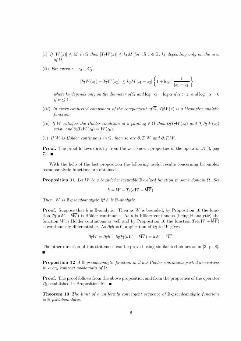
(i) If |W (z)| ≤ M in Ω then |TzW (z)| ≤ k1M for all z ∈ Ω, k1 depending only on the areaof Ω.
(ii) For every z1, z2 ∈ Cj,
|TzW (z1)− TzW (z2)| ≤ k2M |z1 − z2|
1 + log+
1
|z1 − z2|
where k2 depends only on the diameter of Ω and log+ α = log α if α > 1, and log+ α = 0if α ≤ 1.
(iii) In every connected component of the complement of Ω, TzW (z) is a bicomplex analyticfunction.
(iv) If W satisfies the Holder condition at a point z0 ∈ Ω then ∂zTzW (z0) and ∂zTzW (z0)exist, and ∂zTzW (z0) =W (z0).
(v) If W is Holder continuous in Ω, then so are ∂zTzW and ∂zTzW .
Proof. The proof follows directly from the well known properties of the operator A [3, pag7].
With the help of the last proposition the following useful results concerning bicomplexpseudoanalytic functions are obtained.
Proposition 11 Let W be a bounded measurable B-valued function in some domain Ω. Set
h =W − Tz(aW + bW ).
Then, W is B-pseudoanalytic iff h is B-analytic.
Proof. Suppose that h is B-analytic. Then as W is bounded, by Proposition 10 the func-tion Tz(aW + bW ) is Holder continuous. As h is Holder continuous (being B-analytic) thefunction W is Holder continuous as well and by Proposition 10 the function Tz(aW + bW )is continuously differentiable. As ∂zh = 0, application of ∂z to W gives
∂zW = ∂zh+ ∂zTz(aW + bW ) = aW + bW .
The other direction of this statement can be proved using similar techniques as in [3, p. 8].
Proposition 12 A B-pseudoanalytic function in Ω has Holder continuous partial derivativesin every compact subdomain of Ω.
Proof. The proof follows from the above proposition and from the properties of the operatorTz established in Proposition 10.
Theorem 13 The limit of a uniformly convergent sequence of B-pseudoanalytic functionsis B-pseudoanalytic.
9

Proof. Let Wn(z) be a sequence of bounded B-pseudoanalytic functions in a boundeddomain Ω such that Wn(z) →W (z) uniformly in Ω. It follows from Proposition 11 that thefunctions hn defined by
hn =Wn − Tz(aWn + bWn)
are B-analytic in Ω. Then the uniform limit h = W − Tz(aW + bW ) is also a B-analyticfunction in Ω. The last equality together with Proposition 11 allows one to conclude thatW is B-pseudoanalytic in Ω.
Theorem 14 Let W be a B-pseudoanalytic function in Ω except perhaps a finite numberof points z1, .., zp where W is allowed to be unbounded. Then if W−1W is a boundedmeasurable function in Ω, there exists a B-analytic function Ψ in Ω\ z1, .., zp such that
W = ΨE [S] , in Ω,
where S = Tz(a+WWb).
Proof. Application of ∂z to Ψ =WE [−S] gives
∂zΨ = (∂zW )E [−S] +W∂zE [−S]
=(aW + bW
)E [−S] +W
(−a−
W
Wb
)E [−S] = 0.
Then Ψ is B-analytic.
3.2 Vekua’s equation for (F,G)-derivatives and the antiderivative
Definition 15 Let (F,G) and (F1, G1) be two generating pairs in Ω. (F1, G1) is called asuccessor of (F,G) and (F,G) is called a predecessor of (F1, G1) if
a(F1,G1) = a(F,G) and b(F1,G1) = −B(F,G).
By analogy with the complex case [3] (see also [16]) we have the following statements
Theorem 16 Let W be a bicomplex (F,G)-pseudoanalytic function and let (F1, G1) be a
successor of (F,G). ThenW is an (F1, G1)-pseudoanalytic function.
Definition 17 A sequence of generating pairs (Fm, Gm), m = 0,±1,±2, . . . is called agenerating sequence if (Fm+1, Gm+1) is a successor of (Fm, Gm). If (F0, G0) = (F,G), wesay that (F,G) is embedded in (Fm, Gm).
Let W be a bicomplex (F,G)-pseudoanalytic function. Using a generating sequence inwhich (F,G) is embedded we can define the higher derivatives ofW by the recursion formula
W [0] =W ; W [m+1] =d(Fm,Gm)W
[m]
dz, m = 0, 1, . . . .
10
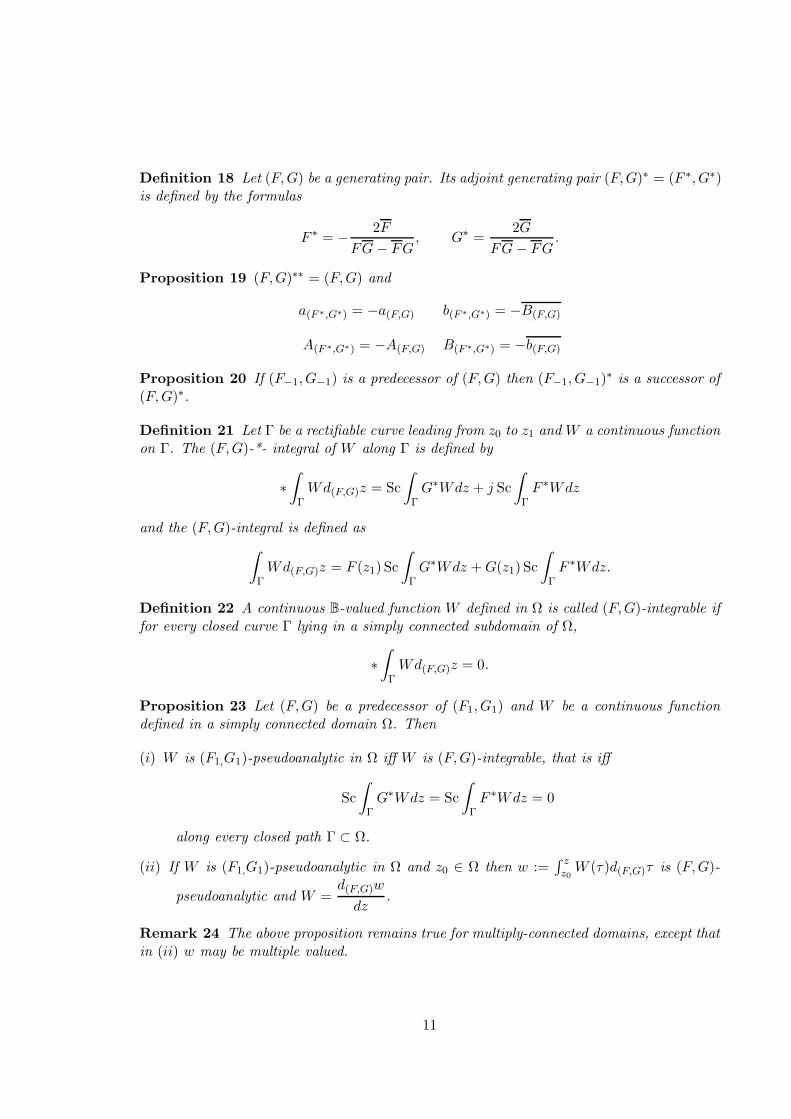
Definition 18 Let (F,G) be a generating pair. Its adjoint generating pair (F,G)∗ = (F ∗, G∗)is defined by the formulas
F ∗ = −2F
FG− FG, G∗ =
2G
FG− FG.
Proposition 19 (F,G)∗∗ = (F,G) and
a(F ∗,G∗) = −a(F,G) b(F ∗,G∗) = −B(F,G)
A(F ∗,G∗) = −A(F,G) B(F ∗,G∗) = −b(F,G)
Proposition 20 If (F−1, G−1) is a predecessor of (F,G) then (F−1, G−1)∗ is a successor of
(F,G)∗.
Definition 21 Let Γ be a rectifiable curve leading from z0 to z1 andW a continuous functionon Γ. The (F,G)-*- integral of W along Γ is defined by
∗
∫
ΓWd(F,G)z = Sc
∫
ΓG∗Wdz + j Sc
∫
ΓF ∗Wdz
and the (F,G)-integral is defined as
∫
ΓWd(F,G)z = F (z1) Sc
∫
ΓG∗Wdz +G(z1) Sc
∫
ΓF ∗Wdz.
Definition 22 A continuous B-valued function W defined in Ω is called (F,G)-integrable iffor every closed curve Γ lying in a simply connected subdomain of Ω,
∗
∫
ΓWd(F,G)z = 0.
Proposition 23 Let (F,G) be a predecessor of (F1, G1) and W be a continuous functiondefined in a simply connected domain Ω. Then
(i) W is (F1,G1)-pseudoanalytic in Ω iff W is (F,G)-integrable, that is iff
Sc
∫
ΓG∗Wdz = Sc
∫
ΓF ∗Wdz = 0
along every closed path Γ ⊂ Ω.
(ii) If W is (F1,G1)-pseudoanalytic in Ω and z0 ∈ Ω then w :=∫ z
z0W (τ)d(F,G)τ is (F,G)-
pseudoanalytic and W =d(F,G)w
dz.
Remark 24 The above proposition remains true for multiply-connected domains, except thatin (ii) w may be multiple valued.
11
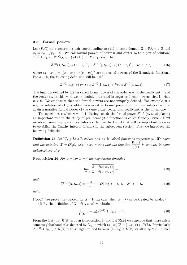
3.3 Formal powers
Let (F,G) be a generating pair corresponding to (11) in some domain Ω ⊂ R2, n ∈ Z and
z0 = x0 + jy0 ∈ Ω. We call formal powers of order n and center z0 to a pair of solutionsZ(n)(1, z0, z), Z
(n)(j, z0, z) of (11) in Ω\ z0 such that
Z(n)(1, z0, z) ∼ (z − z0)n , Z(n)(j, z0, z) ∼ j (z − z0)
n , as z → z0, (16)
where (z − z0)n = [(x− x0) + j(y − y0)]
n are the usual powers of the B-analytic functions.For α ∈ B, the following definition will be useful
Z(n)(α, z0, z) := Scα Z(n)(1, z0, z) + Vecα Z(n)(j, z0, z). (17)
The function defined by (17) is called formal power of the order n with the coefficient α andthe center z0. In this work we are mainly interested in negative formal powers, that is whenn < 0. We emphasize that the formal powers are not uniquely defined. For example, if aregular solution of (11) is added to a negative formal power the resulting solution will beagain a negative formal power of the same order, center and coefficient as the initial one.
The special case when n = −1 is distinguished: the formal power Z(−1)(α, z0, z) playingan important role in the study of pseudoanalytic functions is called Cauchy kernel. Nextwe obtain some asymptotic formulas for the Cauchy kernel that will be important in orderto establish the Cauchy integral formula in the subsequent section. First we introduce thefollowing definition.
Definition 25 Let W , g be a B-valued and an R-valued functions respectively. We agree
that the notation W = O(g), as z → z0, means that the functionW (z)
g(z)is bounded in some
neighborhood of z0.
Proposition 26 For α = 1or α = j the asymptotic formulas
limz→z0
∣∣∣∣∣Z(−1)(α, z0, z)
Z(−1)(α, z0, z)
∣∣∣∣∣ = 1 (18)
andZ(−1)(α, z0, z) =
α
z − z0+O( log |z − z0|), as z → z0 (19)
hold.
Proof. We prove the theorem for α = 1, the case when α = j can be treated by analogy.(i) By the definition of Z(−1)(1, z0, z) we obtain
limz→z0
(z − z0)Z(−1)(1, z0, z) = 1. (20)
From the fact that R(B) is open (Proposition 3) and 1 ∈ R(B) we conclude that there existssome neighborhood of z0 denoted by Nz0 in which (z−z0)Z
(−1)(1, z0, z) ∈ R(B). ParticularlyZ(−1)(1, z0, z) ∈ R(B) in this neighborhood because (z−z0) ∈ R(B) for all z, z0 ∈ Cj. Hence
12
the function on the left hand side of (18) is well defined for z ∈ Nz0 . Finally, using (20) andProposition 2 we have
∣∣∣∣∣Z(−1)(1, z0, z)
Z(−1)(1, z0, z)
∣∣∣∣∣ =∣∣∣∣∣(z − z0)
(z − z0)
∣∣∣∣∣
∣∣∣∣∣Z(−1)(1, z0, z)
Z(−1)(1, z0, z)
∣∣∣∣∣ =
=
∣∣∣∣∣(z − z0)
(z − z0)
Z(−1)(1, z0, z)
Z(−1)(1, z0, z)
∣∣∣∣∣ → 1
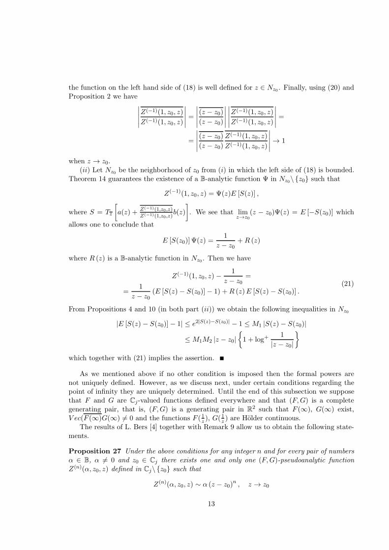
when z → z0.(ii) Let Nz0 be the neighborhood of z0 from (i) in which the left side of (18) is bounded.
Theorem 14 guarantees the existence of a B-analytic function Ψ in Nz0\ z0 such that
Z(−1)(1, z0, z) = Ψ(z)E [S(z)] ,
where S = Tz
[a(z) + Z(−1)(1,z0,z)
Z(−1)(1,z0,z)b(z)
]. We see that lim
z→z0(z − z0)Ψ(z) = E [−S(z0)] which
allows one to conclude that
E [S(z0)] Ψ(z) =1
z − z0+R (z)
where R (z) is a B-analytic function in Nz0 . Then we have
Z(−1)(1, z0, z)−1
z − z0=
=1
z − z0(E [S(z)− S(z0)]− 1) +R (z)E [S(z)− S(z0)] .
(21)
From Propositions 4 and 10 (in both part (ii)) we obtain the following inequalities in Nz0
|E [S(z)− S(z0)]− 1| ≤ e2|S(z)−S(z0)| − 1 ≤M1 |S(z)− S(z0)|
≤M1M2 |z − z0|
1 + log+
1
|z − z0|
which together with (21) implies the assertion.
As we mentioned above if no other condition is imposed then the formal powers arenot uniquely defined. However, as we discuss next, under certain conditions regarding thepoint of infinity they are uniquely determined. Until the end of this subsection we supposethat F and G are Cj-valued functions defined everywhere and that (F,G) is a completegenerating pair, that is, (F,G) is a generating pair in R
2 such that F (∞), G(∞) exist,V ec(F (∞)G(∞) 6= 0 and the functions F (1
z), G(1
z) are Holder continuous.
The results of L. Bers [4] together with Remark 9 allow us to obtain the following state-ments.
Proposition 27 Under the above conditions for any integer n and for every pair of numbersα ∈ B, α 6= 0 and z0 ∈ Cj there exists one and only one (F,G)-pseudoanalytic functionZ(n)(α, z0, z) defined in Cj\ z0 such that
Z(n)(α, z0, z) ∼ α (z − z0)n , z → z0
13

andZ(n)(α, z0, z) = O(|z|n), z → ∞ (22)
and having no other zeros or poles except at z = ∞.
The functions described in the above proposition are called global formal powers. Thenegative global formal powers enjoy the following interesting relations.
Theorem 28 Let (Fm, Gm), m = 0,±1,±2, . . . be a generating sequence of complete gen-
erating pairs in which (F,G) is embedded and Z(−n)m (α, z0, z), Z
∗(−n)m (α, z0, z) denote the
(Fm, Gm)- and the (Fm, Gm)∗- negative formal powers, respectively. Then for any positiveinteger n we have
ScZ(−n)m (j, z0, z) + j ScZ(−n)
m (1, z0, z) = (−1)nZ∗(−n)m−n (j, z, z0)
VecZ(−n)m (j, z0, z) + j VecZ(−n)
m (1, z0, z) = (−1)nZ∗(−n)m−n (1, z, z0).
Due to the above theorem for fixed values of z the global formal powers Z(−n)m (j, z0, z)
are continuously differentiable in the variable z0.There are currently no results regarding the existence or the uniqueness for the global
formal powers of a general bicomplex Vekua equation though in Subsection 4.1 we establishan existence result under certain additional conditions. We end this section by mentioningthat even for complex Vekua equations the construction of the negative formal powers (globalor not) is a very difficult task. In Section 6 we construct the negative formal powers in theexplicit form for some classes of bicomplex main Vekua equations.
3.4 A relation between the Schrodinger equation and the main Vekuaequation
Let q be a complex (Ci-valued) continuous function in Ω ⊆ R2. Consider the two-dimensional
stationary Schrodinger equation
∆u− qu = 0 in Ω (23)
and assume that it possesses a Ci-valued particular solution f ∈ C2(Ω) such that f(z) 6= 0for all z ∈ Ω. We will need a result from [13] (see also [16]) relating the Schrodinger equationwith a Vekua equation of a special kind.
Theorem 29 LetW = u+jv with u = ScW , v = VecW be a solution of the main bicomplexVekua equation
∂zW =∂zf
fW in Ω. (24)
Then u is a solution of (23) and v is a solution of
∆v − q1v = 0 in Ω (25)
where q1 = 2(∂xf)
2+(∂yf)2
f2 − q.
14

Remark 30 A generating pair corresponding to (24) can be chosen in the form
(F,G) = (f,j
f). (26)
The corresponding characteristic coefficients are
a(f, jf) = A(f, j
f) = 0, b(f, j
f) =
∂zf
f, B(f, j
f) =
∂zf
f
and the successor equation of (24) is
∂zW = −∂zf
fW. (27)
We need the following notation. Let W be a B-valued function defined on a simplyconnected domain Ω with u = ScW and v = VecW such that
∂u
∂y−∂v
∂x= 0, in Ω (28)
and let Γ ⊂ Ω be a simple rectifiable curve leading from z0 = x0 + jy0 to z = x+ jy. Thenthe integral
AW (z) := 2
(∫
Γudx+ vdy
)
is path-independent, and all Ci-valued solutions ϕ of the equation ∂zϕ = W in Ω have theform ϕ(z) = AW (z) + c where c is an arbitrary Ci-constant.
Remark 31 It is easy to check that if u is a solution of the Schrodinger equation (23)in a simply connected domain Ω then the B-valued function jf2∂z(f
−1u) satisfies (28) andtherefore the function constructed by the rule
Tf (u) := f−1A(jf2∂z(f−1u)) (29)
is well defined in Ω. Application of Tf to a more general class of functions will be alsoconsidered but as in this case the result of such operation may depend on the choice of thecurve Γ leading from z0 to z, the notation Tf,Γ(u) will be used.
Theorem 32 [14] If u is a Ci-valued solution of the Schrodinger equation (23) in a simplyconnected domain Ω then v = Tf (u) is a solution of (25) and W = u + jv is a solution of(24).
Corollary 33 Let un ∈ C2(Ω) be a sequence of solutions of (23) and u be such that un → u,∂xun → ∂xu and ∂yun → ∂yu uniformly in Ω. Then u is a solution of (23).
Proof. The assumption together with the above theorem allows one to conclude that thesequence of solutions of (24) given by Wn := un + jTf (un) converges uniformly to W :=u + jTf (u). Then by Theorem 13, W is a solution of (24) and from Theorem 29 its scalarpart u is a solution of (23).
15
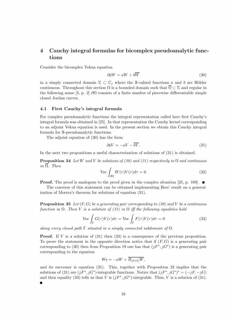
4 Cauchy integral formulas for bicomplex pseudoanalytic func-tions
Consider the bicomplex Vekua equation
∂zW = aW + bW (30)
in a simply connected domain Σ ⊂ Cj where the B-valued functions a and b are Holdercontinuous. Throughout this section Ω is a bounded domain such that Ω ⊂ Σ and regular inthe following sense [3, p. 2] ∂Ω consists of a finite number of piecewise differentiable simpleclosed Jordan curves.
4.1 First Cauchy’s integral formula
For complex pseudoanalytic functions the integral representation called here first Cauchy’sintegral formula was obtained in [25]. In that representation the Cauchy kernel correspondingto an adjoint Vekua equation is used. In the present section we obtain this Cauchy integralformula for B-pseudoanalytic functions.
The adjoint equation of (30) has the form
∂zV = −aV − bV . (31)
In the next two propositions a useful characterization of solutions of (31) is obtained.
Proposition 34 LetW and V be solutions of (30) and (31) respectively in Ω and continuousin Ω. Then
Vec
∫
∂ΩW (τ)V (τ)dτ = 0. (32)
Proof. The proof is analogous to the proof given in the complex situation [25, p. 169].The converse of this statement can be obtained implementing Bers’ result on a general-
ization of Morera’s theorem for solutions of equation (31).
Proposition 35 Let (F,G) be a generating pair corresponding to (30) and V be a continuousfunction in Ω. Then V is a solution of (31) in Ω iff the following equalities hold
Vec
∫
ΓG(τ )V (τ)dτ = Vec
∫
ΓF (τ )V (τ )dτ = 0 (33)
along every closed path Γ situated in a simply connected subdomain of Ω.
Proof. If V is a solution of (31) then (33) is a consequence of the previous proposition.To prove the statement in the opposite direction notice that if (F,G) is a generating paircorresponding to (30) then from Proposition 19 one has that (jF ∗, jG∗) is a generating paircorresponding to the equation
Wz = −aW +B(F,G)W,
and its successor is equation (31). This, together with Proposition 23 implies that thesolutions of (31) are (jF ∗, jG∗)-integrable functions. Notice that (jF ∗, jG∗)∗ = (−jF,−jG)and then equality (33) tells us that V is (jF ∗, jG∗)-integrable. Thus, V is a solution of (31).
16
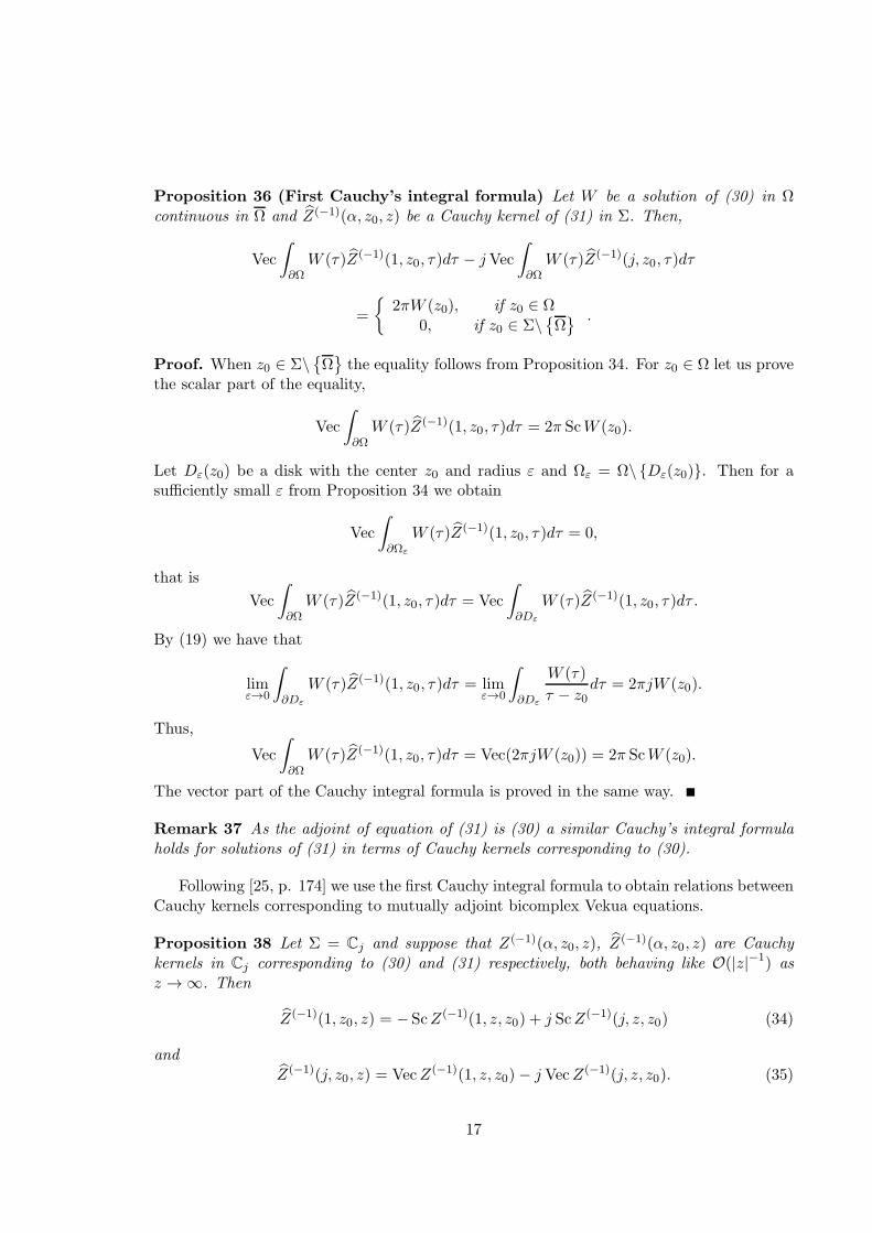
Proposition 36 (First Cauchy’s integral formula) Let W be a solution of (30) in Ωcontinuous in Ω and Z(−1)(α, z0, z) be a Cauchy kernel of (31) in Σ. Then,
Vec
∫
∂ΩW (τ)Z(−1)(1, z0, τ )dτ − jVec
∫
∂ΩW (τ)Z(−1)(j, z0, τ)dτ
=
2πW (z0),
0,
if z0 ∈ Ω
if z0 ∈ Σ\Ω .
Proof. When z0 ∈ Σ\Ωthe equality follows from Proposition 34. For z0 ∈ Ω let us prove
the scalar part of the equality,
Vec
∫
∂ΩW (τ)Z(−1)(1, z0, τ)dτ = 2π ScW (z0).
Let Dε(z0) be a disk with the center z0 and radius ε and Ωε = Ω\ Dε(z0). Then for asufficiently small ε from Proposition 34 we obtain
Vec
∫
∂Ωε
W (τ)Z(−1)(1, z0, τ )dτ = 0,
that is
Vec
∫
∂ΩW (τ)Z(−1)(1, z0, τ )dτ = Vec
∫
∂Dε
W (τ)Z(−1)(1, z0, τ )dτ .
By (19) we have that
limε→0
∫
∂Dε
W (τ)Z(−1)(1, z0, τ )dτ = limε→0
∫
∂Dε
W (τ)
τ − z0dτ = 2πjW (z0).
Thus,
Vec
∫
∂ΩW (τ)Z(−1)(1, z0, τ )dτ = Vec(2πjW (z0)) = 2π ScW (z0).
The vector part of the Cauchy integral formula is proved in the same way.
Remark 37 As the adjoint of equation of (31) is (30) a similar Cauchy’s integral formulaholds for solutions of (31) in terms of Cauchy kernels corresponding to (30).
Following [25, p. 174] we use the first Cauchy integral formula to obtain relations betweenCauchy kernels corresponding to mutually adjoint bicomplex Vekua equations.
Proposition 38 Let Σ = Cj and suppose that Z(−1)(α, z0, z), Z(−1)(α, z0, z) are Cauchy
kernels in Cj corresponding to (30) and (31) respectively, both behaving like O(|z|−1) asz → ∞. Then
Z(−1)(1, z0, z) = − ScZ(−1)(1, z, z0) + j ScZ(−1)(j, z, z0) (34)
andZ(−1)(j, z0, z) = VecZ(−1)(1, z, z0)− j VecZ(−1)(j, z, z0). (35)
17
Proof. Let z0, z ∈ Cj, z0 6= z and ε > 0 be sufficiently small such that z ∈ Ωε =D 1
ε(z0)\Dε(z0) where Dε(z0) is a disc with the center z0 and radius ε. Then from the
first Cauchy integral formula we have
2πZ(−1)(1, z0, z)
= Vec
∫
∂Ωε
Z(−1)(1, z0, τ )Z(−1)(1, z, τ )dτ − jVec
∫
∂Ωε
Z(−1)(1, z0, τ)Z(−1)(j, z, τ )dτ
or equivalently,
2πZ(−1)(1, z0, z)
= Vec
∫
∂D 1ε
Z(−1)(1, z0, τ)Z(−1)(1, z, τ )dτ − j Vec
∫
∂D 1ε
Z(−1)(1, z0, τ )Z(−1)(j, z, τ )dτ
−Vec
∫
∂Dε
Z(−1)(1, z0, τ)Z(−1)(1, z, τ )dτ + j Vec
∫
∂Dε
Z(−1)(1, z0, τ )Z(−1)(j, z, τ )dτ.
Taking into account the asymptotic behaviour of the kernels at infinity it is easy to verifythat the first and the second integrals on the right-hand side of the equality tends to zerowhen ε→ 0. Then (34) is obtained from the last equality applying the first Cauchy integralformula to the last two integrals and considering ε→ 0. A similar reasoning proves (35).
Remark 39 Under the assumptions of Proposition 27 (which in particular imply that a andb are Cj-valued functions) equations (30) and (31) possess unique Cauchy kernels (calledglobal Cauchy kernels) satisfying the conditions of Proposition 38 and therefore they canbe computed one from another by means of (34) and (35). For a general bicomplex Vekuaequation we were not able to obtain comparable definitive results regarding the existence oruniqueness of the kernels possessing such properties. However from the previous propositionwe immediately obtain the following uniqueness result.
Corollary 40 If both equations (30) and (31) possess Cauchy kernels fulfilling the assump-tions of Proposition 38 then they are unique.
4.2 Second Cauchy’s integral formula and reproducing Cauchy kernels
Definition 41 Let Ω ⊆ Σ be a regular domain, W be a continuous function up to Ω andZ(n)(α, z0, z) be a formal power corresponding to (30) in Σ, continuous in the variable z0 forfixed values of z. Following [3] we define
∫
∂ΩZ(n)(jW (τ )dτ , τ , z0) =
∫ b
a
Z(n)(jW (γ(t))γ ′(t)dt, γ(t), z0)
where γ(t) : [a, b] → Cj is a parametrization of ∂Ω.
Theorem 42 (Second Cauchy’s integral formula) [25] Let Z(−1)(α, z0, z), Z(−1)(α, z0, z)
be Cauchy kernels corresponding to (30) and (31) respectively satisfying (34), (35) in Σ andW be a solution of (30) in Ω continuous in Ω. Then
∫
∂ΩZ(−1)(jW (τ )dτ , τ , z0) = 2πW (z0), (36)
18
for z0 ∈ Ω and ∫
∂ΩZ(−1)(jW (τ )dτ, τ , z0) = 0 (37)
for z0 ∈ Σ\Ω.
Proof. Direct calculation gives us the equality
∫
∂ΩZ(−1)(jW (τ)dτ , τ , z0) =
= Vec
∫
∂ΩW (τ)
− ScZ(−1)(1, τ , z0) + j ScZ(−1)(j, τ , z0)
dτ (38)
− j Vec
∫
∂ΩW (τ)
VecZ(−1)(1, τ , z0)− j VecZ(−1)(j, τ , z0)
dτ .
From (34), (35), (38) and from the first Cauchy integral formula we obtain the result.
Remark 43 Formulas (36) and (37) were obtained independently in [3] and [25] using globalCauchy kernels. Our proof which follows that from [25] reveals that the second Cauchyintegral formula is equivalent to the first when an appropriate Cauchy kernel corresponding to(30) is used. The Cauchy kernels involved, Z(−1)(α, z0, z) and Z(−1)(α, z0, z) should satisfyequalities (34), (35) in the domain of interest but not necessarily be global. It is worthnoticing that equalities (36) and (37) are not valid for an arbitrary Cauchy kernel of (30).For example, consider the following Cauchy kernels
Z(−1)(1, ζ, z) =1
z − ζ+ ξ, Z(−1)(j, ζ, z) =
j
z − ζ.
of the equation ∂zW = 0, where z = x+ jy and ζ = ξ + jη. If Ω is the unitary disk, z0 = 0and W ≡ 1 then the left-hand side of (36) is
2π∫
0
Z(−1)(j2ejθdθ, ejθ, 0) = −
2π∫
0
[(cos θ)Z(−1)(1, ejθ, 0) + (sin θ)Z(−1)(j, ejθ, 0)
]dθ
=
2π∫
0
(1− cos2 θ)dθ = π
which is different from 2πW (0).
Definition 44 We say that a Cauchy kernel Z(−1)(α, z0, z) defined in Σ reproduces a solu-tion W of (30) if for every domain Ω where W is pseudoanalytic in Ω and continuous inΩ the formula (36) holds. A local Cauchy kernel is called reproducing if it reproduces allsolutions of (30).
Combining results of the preceding sections we obtain the following criteria describingthe reproducing Cauchy kernels.
19
Theorem 45 Let (F,G) be a generating pair and Z(−1)(α, z0, z) be a Cauchy kernel, bothcorresponding to (30) in Σ and such that for each fixed z the kernel Z(−1)(α, z0, z) is acontinuous function in the variable z0 and
limz0→z
(z − z0)Z(−1)(α, z0, z) = α, α = 1, j. (39)
Then the following statements are equivalent:
(i) Z(−1)(α, z0, z) reproduces both solutions F and G;
(ii) There exists a Cauchy kernel Z(−1)(α, z0, z) corresponding to (31) such that (34) and(35) hold;
(iii) Second Cauchy’s integral formula holds;
(iv) Z(−1)(α, z0, z) is a reproducing Cauchy kernel.
Proof.
(i) ⇒ (ii) Let z0 ∈ Σ and Ω be a domain such that z0 /∈ Ω ⊂ Σ. Then from (i) we have
∫
∂ΩZ(−1)(jF (τ )dτ , τ , z0) =
∫
∂ΩZ(−1)(jG(τ )dτ, τ , z0) = 0.
From this equality and from (38) we obtain
Vec
∫
∂ΩF (τ)w1,2(z0, τ)dτ = Vec
∫
∂ΩG(τ )w1,2(z0, τ )dτ = 0 (40)
where
w1(z0, z) := − ScZ(−1)(1, z, z0) + j ScZ(−1)(j, z, z0),
w2(z0, z) := VecZ(−1)(1, z, z0)− jVecZ(−1)(j, z, z0).
From (40) and Proposition 35 we conclude that w1,2(z0, z) are solutions of (31) inΩ\z0. On the other hand using (39) we see that the left-hand side of these equalitiesdefines Cauchy kernels corresponding to (31). Thus, (34) and (35) hold.
(ii) =⇒ (iii) follows from Theorem 42.
(iii) ⇒ (iv) and (iv) ⇒ (i) is straightforward.
In the following example we slightly change the Cauchy kernel from Remark 43 andobtain a reproducing but not global Cauchy kernel.
Example 46 Consider the Cauchy kernel
Z(−1)(1, ζ, z) =1
z − ζ+ ξ, Z(−1)(j, ζ, z) =
j
z − ζ+ η
20
corresponding to the equation ∂zW = 0 with ζ = ξ + jη. Since
− ScZ(−1)(1, z, z0) + j ScZ(−1)(j, z, z0) =1
z − z0+ z (41)
and
VecZ(−1)(1, z, z0)− j VecZ(−1)(j, z, z0) =1
z − z0, (42)
due to Theorem 45 Z(−1)(α, ζ, z) is a reproducing Cauchy kernel in any bounded domain.Let us prove that this kernel is not a restriction of any global Cauchy kernel in any simply
connected domain containing (0, 0) and (1, 0) as interior points. Indeed, take ζ = 1+ 1nand
z = ζ − 1ξ= 1 + 1
n− n
n+1 . Then Z(−1)(1, ζ, z) = 0. On the other hand as we know a globalCauchy kernel can not vanish except at z = ∞.
5 Construction of negative formal powers
Let(Fn, Gn
), n = 0, 1, 2 . . . be a generating sequence in a domain Σ ⊂ Cj embedding a
generating pair corresponding to (31). In this section we show how a set of negative formalpowers corresponding to (30) can be constructed following a simple algorithm when the
sequence(Fn, Gn
)and a reproducing Cauchy kernel for (30) are known.
Let Z(−1)(α, z0, z) be a reproducing Cauchy kernel of (30) enjoying the properties fromthe hypothesis of Theorem 45. Then, as was established in Theorem 45, Z(−1)(α, z0, z)constructed by means of (34) and (35) is a reproducing Cauchy kernel for (31). For aninteger n ≥ 2 define
Z(−n)n−1 (α, z0, z) :=
(−1)n−1
(n − 1)!
d(Fn−2,Gn−2)
dz...d(F1,G1)
dz
d(F0,G0)
dzZ(−1)(α, z0, z).
By construction, Z(−n)n−1 (α, z0, z) is an
(Fn−1, Gn−1
)-formal power of the order −n. These
are related with the formal powers for equation (30) in the following way.
Theorem 47 Under the above conditions suppose that the functions Z(−n)n−1 (α, z0, z), α = 1, j
are continuous in the variable z0 for fixed values of z and that
limz0→z
(z − z0)nZ
(−n)n−1 (α, z0, z) = α, α = 1, j. (43)
ThenZ(−n)(1, z0, z) := (−1)n Sc Z
(−n)n−1 (1, z, z0) + j(−1)n+1 Sc Z
(−n)n−1 (j, z, z0), (44)
Z(−n)(j, z0, z) := (−1)n+1 Vec Z(−n)n−1 (1, z, z0) + j(−1)n Vec Z
(−n)n−1 (j, z, z0) (45)
are negative formal powers corresponding to (30).
Proof. Let z0 ∈ Σ and Ω be a domain such that z0 /∈ Ω ⊂ Σ. As mentioned aboveZ(−1)(α, z0, z) constructed by means of (34) and (35) is a reproducing Cauchy kernel corre-sponding to (31). This in particular implies that
∫
∂ΩZ(−1)(jF (τ )dτ, τ , z0) =
∫
∂ΩZ(−1)(jG(τ )dτ , τ , z0) = 0.
21

Taking in the above equalities n − 1 Bers’ derivatives with respect to the variable z0 weobtain ∫
∂ΩZ
(−n)n−1 (jF (τ)dτ , τ , z0) =
∫
∂ΩZ
(−n)n−1 (jG(τ)dτ , τ , z0) = 0
which equivalently can be written as follows
Vec
∫
∂ΩF (τ )w1,2(z0, τ)dτ = Vec
∫
∂ΩG(τ)w1,2(z0, τ )dτ = 0, (46)
wherew1(z0, z) := − Sc Z
(−n)n−1 (1, z, z0) + j Sc Z
(−n)n−1 (j, z, z0),
w2(z0, z) := Vec Z(−n)n−1 (1, z, z0)− j Vec Z
(−n)n−1 (j, z, z0).
Equalities (46) together with Proposition 35 allow one to conclude that w1,2(z0, z) aresolutions of (30) in Ω\z0. On the other hand, using (43) we see that the left-hand side of(44) and (45) defines formal powers corresponding to (30).
Remark 48 The generating sequence(Fn, Gn
)required in the above construction can
be obtained as follows. Let (F−n, G−n), n = 0, 1, 2 . . . be a generating sequence embed-
ding a generating pair corresponding to (30). Then by Propositions 19 and 20,(F , G
):=
(jF ∗−1, jG
∗−1) is a generating pair for (31) embedded in the generating sequence
(Fn, Gn
),
n = 0, 1, 2 . . . where(Fn, Gn
):= (j (F−n−1)
∗ , j (G−n−1)∗).
Remark 49 Let us mention that if (F−n, G−n), n = 0, 1, 2 . . . is a complete generatingsequence of Cj-valued generating pairs then by Theorem 28 the corresponding (F,G)- and(Fn, Gn
)- negative global formal powers satisfy (44) and (45).
6 Applications to the main Vekua and Schrodinger equations
Let us suppose that the Schrodinger equation (23) has a nonvanishing particular Ci-valuedsolution f ∈ C2(Ω). Then as it was explained in Section 3.3 the main Vekua equation (24)is closely related to the Schrodinger equation (23). In this section we use this relation forobtaining the following results. Starting from a fundamental solution of (23) we constructexplicitly a reproducing kernel and corresponding negative formal powers for (24) as well asa fundamental solution for the Darboux transformed equation (25).
Definition 50 We say that a function M(ζ, z) satisfies condition I in Ω × Ω if M(ζ, z)together with its first partial derivatives corresponding to ζ are continuous functions in Ω×Ω\ diag, M(ζ, z) is bounded in some neighborhood of every point (z0, z0) and the samepartial derivatives behave like O(log |z − ζ|) as (ζ, z) → (z0, z0).
We are mainly interested in fundamental solutions for (23)
S(ζ, z) = log |z − ζ|+R(ζ, z)
fulfilling the following conditions:
22
(C1) S(z, ζ) is a solution of (23) in both variables z and ζ;
(C2) R(ζ, z) ∈ C1(Ω × Ω\ diag) and R is bounded in some neighborhood of every point(z0,z0), z0 ∈ Ω.
(C3) The functions ∂xR(ζ, z), ∂yR(ζ, z) satisfy the condition I in Ω× Ω.
6.1 Construction of a reproducing Cauchy kernel
The purpose of this subsection is to construct a reproducing kernel for the main Vekuaequation (24) from a fundamental solution of (23). First we notice the following fact.
Proposition 51 Under the choice of the generating pair corresponding to (24) in the form(26) the successor and the adjoint equation for (24) coincide.
Proof. This is a direct consequence of Remark 30.This observation together with Theorem 45 allow us to state that Z(−1)(α, ζ, z) is a
reproducing kernel for (24) when the formulas
Z(−1)1 (1, ζ, z) = − ScZ(−1)(1, z, ζ) + j ScZ(−1)(j, z, ζ), (47)
Z(−1)1 (j, ζ, z) = VecZ(−1)(1, z, ζ)− j VecZ(−1)(j, z, ζ). (48)
hold where Z(−1)1 (α, ζ, z) is some Cauchy kernel of (27). We will start by constructing
Z(−1)1 (1, ζ, z) and then the above formulas can be used to obtain Z
(−1)1 (j, ζ, z) and Z(−1)(α, ζ, z).
Proposition 52 Let S(ζ, z) be a fundamental solution of (23) satisfying (C1)− (C3). Thenthe function defined as follows
Z(−1)1 (1, ζ, z) := 2(∂zS(ζ, z) −
∂zf(z)
f(z)S(ζ, z)) (49)
satisfies the following properties:
(i)
Z(−1)1 (1, ζ, z) =
1
z − ζ− 2
∂zf(z)
f(z)log |z − ζ|+M(ζ, z), (50)
where M(ζ, z) satisfies condition I.
(ii) Z(−1)1 (1, ζ, z) is a Cauchy kernel of (27);
(iii) The scalar and the vector parts of Z(−1)1 (1, ζ, z) are solutions of (23) in the variable ζ.
Proof. (i) Equality (50) and the properties of M follow directly from (49) and from theconditions (C1)− (C3) defining the fundamental solution S.
(ii) By construction Z(−1)1 (1, ζ, z) is a solution of (27) and from (50) we have
limz→ζ
(z − ζ)Z(−1)1 (1, ζ, z) = 1,
23

from which we conclude that this function is a Cauchy kernel.(iii) We prove that the scalar part of (49)
ScZ(−1)1 (1, ζ, z) = ∂xS(ζ, z)−
fx(z)
f(z)S(ζ, z)
is a solution of (23) in the variable ζ. As S(ζ, z) is already a solution of (23) with respect toζ, it is sufficient to prove that ∂xS(ζ, z) is a solution of the same equation in ζ. We give arigorous proof of this fact. Let z0 = x0 + jy0 ∈ Ω and define ϕ(ζ) = ∂xS(ζ, z0),
ϕn(ζ) =S(ζ, z0 +
1n)− S(ζ, z0)1n
, n ∈ N.
Each function ϕn(ζ) is a solution of (23) and ϕn(ζ) → ϕ(ζ) pointwise. Let ζ0 ∈ Ω, ζ0 6= z0.We will prove that
ϕn(ζ) → ϕ(ζ), ∂ξϕn(ζ) → ∂ξϕ(ζ) and ∂ηϕn(ζ) → ∂ηϕ(ζ)
uniformly is some neighborhood of ζ0. This together with Corollary 33 allows us to concludethat ϕ(ζ) is a solution of (23) in such neighborhood of ζ0, and also in Ω\ z0 (because ζ0 isan arbitrary point).
By the mean value theorem there exists some point xn ∈[x0,x0 +
1n
]such that
ϕn(ζ) = ∂xS(ζ, xn + jy0)
Let ε > 0. Then by the continuity of ∂xS in Ω × Ω\ diag there exist r > 0 and n0 ∈ N
such that|ϕ(ζ)− ϕn(ζ)| = |∂xS(ζ, z0)− ∂xS(ζ, xn + jy0)| < ε
for all ζ belonging to the disk Dr(ζ0) of radius r and center ζ0 and n ≥ n0. This showsthat ϕn(ζ) → ϕ(ζ) uniformly in Dr(ζ0). Let us now prove ∂ξϕn(ζ) → ∂ξϕ(ζ). From thecontinuity of ∂ξ∂xS in Ω×Ω\ diag and using the mean value theorem we have that thereexists xn ∈
[x0,x0 +
1n
]such that
∂ξϕn(ζ) =∂ξS(ζ, z0 +
1n)− ∂ξS(ζ, z0)1n
= ∂x∂ξS(ζ, xn + iy0)
= ∂ξ∂xS(ζ, xn + iy0).
As above, given ε > 0 we can find some r such that
|∂ξϕn(ζ)− ∂ξϕ(ζ)| = |∂ξ∂xS(ζ, xn + iy0)− ∂ξ∂xS(ζ, z0)| < ε
for all ζ ∈ Dr(ζ0) which implies that ∂ξϕn(ζ) → ∂ξϕ(ζ) uniformly in Dr(ζ0). The cor-responding convergence for the partial derivatives with respect to η is proved analogously.
Formulas (47), (48) together with (iii) of the above proposition suggest that a Cauchykernel of (27) with the coefficient α = j can be constructed from (49) according to theformula
Z(−1)1 (j, ζ, z) := Tf(ζ)(−Z
(−1)1 (1, ζ, z)). (51)
24
where the integral operator Tf(ζ) (defined by (29)) acts with respect to the variable ζ alongsome path Γ ⊂ Ω joining ζ0 with ζ and not passing through the point z. We prove this factin the following proposition.
Proposition 53 Let Z(−1)1 (1, ζ, z) be the Cauchy kernel of (27) given by (49), ζ0 ∈ Ω and
Ω0 be a simply connected subdomain of Ω such that ζ0 /∈ Ω0. Then
(i) the function (51) is a Cauchy kernel with the coefficient j for equation (49) in Ω0
(ii) the scalar and the vector parts of Z(−1)1 (j, ζ, z) are solutions of (25) in the variable ζ
(iii) the equality holds
Z(−1)1 (j, ζ, z) =
j
z − ζ+ 2j
∂zf(z)
f(z)log |z − ζ|+N(ζ, z) (52)
where N(ζ, z) is a function satisfying condition I in Ω0.
Proof. It follows from (iii) of Proposition 52 and from Remark 31 that (51) is a well definedfunction when ζ belongs to any simply connected subdomain of Ω0 not containing z. Sincethe function M(ζ, z) in (50) satisfies condition I, it is easy to see that
limε→0
Tf(ζ),Γε(−Z
(−1)1 (1, ζ, z)) = 0
where Γε is the boundary of a disk with the center z and radius ε. This implies that (51) isa univalued function in Ω0\ z. Then (ii) of this proposition follows from Theorem 32.
Let us prove (iii). It is clear that the function N(ζ, z) in (52) together with its firstpartial derivatives corresponding to ζ are continuous functions in Ω0×Ω0\ diag. It remainsto study the behavior of N(ζ, z) and of its partial derivatives corresponding to ζ when(ζ, z) → (z0, z0) ∈ Ω0 × Ω0. Consider the scalar part of N(ζ, z),
ScN(ζ, z) = Tf(ζ)(− ScZ(−1)1 (1, ζ, z))−
y − η
|z − ξ|2−∂yf(z)
f(z)log |z − ξ| . (53)
Let z0 ∈ Ω0, ε0 > 0 such that D2ε0(z0) ⊂ Ω0 and ζ = ξ + jη, z = x+ jy ∈ Dε0(z0). Considerthe path Γ = Γ1 ∪ Γ2 ∪ Γ3 where Γ1 is some rectifiable curve joining ζ0 with z + ε0 and notpassing through the point z, and
Γ2(t) = t+ jy, t ∈ [x+ ε0, x+ |ζ − z|] ,
Γ3(t) = z + |ζ − z| ejt, t ∈ [0, arg(ζ − z)] .
It is clear that Γ leads from ζ0 to ζ and Γ2 ∪ Γ3 ⊂ Ω0. We have
Tf(ζ),Γ(− ScZ(−1)1 (1, ζ, z)) =
3∑
m=1
Tf(ζ),Γm(− ScZ
(−1)1 (1, ζ, z)), (54)
where
ScZ(−1)1 (1, ζ, z) =
x− ξ
|z − ξ|2−fx(z)
f(z)log |z − ξ|+ ScM(ζ, z).
25
The function Tf(ζ),Γ1(− ScZ
(−1)1 (1, ζ, z)) is continuous (since z /∈ Γ1) then and as ScM(ζ, z)
satisfies condition I, the function Tf(ζ),Γ2∪Γ3(− ScM(ζ, z)) is bounded in some neighborhood
of (z0, z0). The remaining terms of (54) are
Tf(ζ),Γ2
(ξ − x
|z − ξ|2+fx(z)
f(z)log |z − ξ|
)=fη(z + |ζ − z|)
f(ζ)log |z − ξ| −
fη(z + ε0)
f(ζ)log ε0
+1
f(ζ)
∫ x+|z−ξ|
x+ε0
(fx(z)
f(z)fη(t+ iy)− fζη(t+ iy)
)log |t− x| dt,
Tf(ζ),Γ3
(ξ − x
|z − ξ|2
)=
y − η
|z − ξ|2−
1
f(ζ)
arg(ξ−z)∫
0
fξ(Γ3(t))dt
and
Tf(ζ),Γ3(log |z − ξ|) =
1
f(ζ)
∫ arg(ξ−z)
0f(Γ3(t))dt
−|z − ζ| log |z − ζ|
f(ζ)
∫ arg(ξ−z)
0(fη(Γ3(t)) sin t+ fξ(Γ3(t) cos t) dt.
Substituting these relations on the right-hand side of (53) we conclude that the functionScN(ζ, z) is bounded when (ζ, z) → (z0, z0). Differentiating (53) with respect to ξ and usingthe relation
∂ξTf(ζ)(− ScZ(−1)1 (1, ζ, z)) = −
fξ(ζ)f(ζ) Tf(ζ)(− ScZ
(−1)1 (1, ζ, z))
−fη(ζ)f(ζ) ScZ
(−1)1 (1, ζ, z) + ∂η ScZ
(−1)1 (1, ζ, z)
we obtain that ∂ξ ScN(ζ, z) = O(|log |z − ζ||) as (ζ, z) → (z0, z0). A similar reasoning canbe used to establish that ∂η ScN(ζ, z) = O(|log |z − ζ||) as (ζ, z) → (z0, z0). This shows thatScN(ζ, z) satisfies condition I in Ω0. An analogous reasoning is applicable to VecN(ζ, z)that finishes the proof of part (iii).
Finally, we prove that (51) is a solution of (27) in the variable z. This together with
(52) will imply (i). Using the fact that Z(−1)1 (1, ζ, z) is a solution of (27) and with the
help of Theorem 13 we can prove, reasoning as in Proposition 52, that ∂ξZ(−1)1 (1, ζ, z),
∂ηZ(−1)1 (1, ζ, z) are also solutions of (27) in z. Then the fact that (51) is a solution of (27)
is obtained from the integration with respect to ζ of solutions of (27) in the variable z. Theproposition is proved.
Example 54 Let f = x. Consider the corresponding main Vekua equation ∂zW = 12xW
in some domain Ω such that Ω has no common point with the axis x = 0. The successorequation has the form
∂zW = −1
2xW (55)
26
and the related Schrodinger equations are ∆u = 0 and ∆v = 2x2 v. A fundamental solution
for the Laplace equation satisfying (C1) − (C3) can be chosen as S(ζ, z) = log |z − ζ|. Areproducing Cauchy kernel for (55) is obtained by means of the procedure described aboveand has the following form
Z(−1)1 (1, ζ, z) =
1
z − ζ−
1
xlog |z − ζ| , (56)
Z(−1)1 (j, ζ, z) =
j
z − ζ+y − η
xξ(log |z − ζ| − 1) +
j
ξlog |z − ζ|
−f(ζ0)
f(ζ)
(j
z − ζ0+y − η0xξ0
(log |z − ζ0| − 1) +j
ξ0log |z − ζ0|
)
where z = x+ jy, ζ = ξ + jη and ζ0 = ξ0 + jη0 ∈ Ω is some fixed point. Here the functioninside the brackets is a regular solution of (55) for z belonging to a domain not containingζ0. Therefore
Z(−1)1 (j, ζ, z) =
j
z − ζ+y − η
xξ(log |z − ζ| − 1) +
j
ξlog |z − ζ| (57)
is a Cauchy kernel of (55) as well. Using Theorem 45 it is easy to verify that the expres-sions (56) and (57) also represent a reproducing Cauchy kernel for (55). The correspondingreproducing Cauchy kernel for the main Vekua equation such that (47) and (48) hold has theform
Z(−1)(1, ζ, z) =1
z − ζ+
1
ξlog |z − ζ| − j
y − η
xξ(log |z − ζ| − 1), (58)
Z(−1)(j, ζ, z) =j
z − ζ− j
1
xlog |z − ζ| . (59)
6.2 Construction of negative formal powers for main Vekua equations
In this subsection we explain how a set of negative formal powers for equation (24) can beconstructed from a fundamental solution of (23) satisfying properties (C1) − (C2). In theprevious section a reproducing Cauchy kernel for equation (24) was constructed. Then, aswas shown in Section 5, using such Cauchy kernel and by means of formulas (44), (45) a set ofnegative formal powers for (24) can be obtained whenever a generating sequence embedding(F , G) is known, where (F , G) is a generating pair corresponding to the adjoint equationof (24). Notice that (f, j
f) is a generating pair for (24) and by Proposition 51 (F , G) is a
successor of (f, jf). Hence it is sufficient to know a generating sequence embedding (f, j
f).
As was shown in [3] (see also [16]) when f has a separable form f = φ(x)ψ(y) where φ andψ are arbitrary twice continuously differentiable functions, there exists a periodic generatingsequence with a period two in which (f, j
f) is embedded,
(F,G) =
(φψ,
j
φψ
), (F1, G1) =
(ψ
φ,jφ
ψ
), (F2, G2) = (F,G) , (F3, G3) = (F1, G1), . . .
(methods for construction of generating sequences in more general situations are discussedin [15], [16] and [18]).
27

Example 55 Consider f = x and the corresponding main Vekua equation ∂zW = 12xW .
The negative formal powers constructed according to the described above procedure beginningwith the reproducing Cauchy kernel (58), (59) have the form
Z(−2)(1, ζ, z) =1
(z − ζ)2+j
xVec
1
z − ζ,
Z(−2)(j, ζ, z) =j
(z − ζ)2−
1
ξ
j
z − ζ+j
x
(Vec
1
z − ζ+
1
ξlog |z − ζ|
),
for an odd n ≥ 3
Z(−n)(1, ζ, z) =1
(z − ζ)n−
1
(n− 1)ξ
1
(z − ζ)n−1−j
(n− 1)xSc
(j
(z − ζ)n−1 −1
(n− 2)ξ
j
(z − ζ)n−2
),
Z(−n)(j, ζ, z) =j
(z − ζ)n−
j
(n− 1)xSc
1
(z − ζ)n−1
and for an even n ≥ 4
Z(−n)(1, ζ, z) =1
(z − ζ)n+
j
(n− 1)xVec
1
(z − ζ)n−1 ,
Z(−n)(j, ζ, z) =j
(z − ζ)n−
1
(n− 1)ξ
j
(z − ζ)n−1+j
(n− 1)xVec
(j
(z − ζ)n−1 −1
(n− 2)ξ
j
(z − ζ)n−2
).
6.3 Construction of fundamental solutions using the Darboux-type trans-formation
Let f ∈ C2(Ω) be a nonvanishing particular solution of (23). Consider the operator Tfdefined by (29) that transforms regular solutions of (23) into regular solutions of the Darbouxtransformed equation (25). We stress that direct application of Tf to a fundamental solutionof (23) does not lead to a fundamental solution of (25). The result rather should be amultivalued solution of (25) with the behaviour similar to that of arg(z − ζ) (the imaginarypart of the function ln(z − ζ)). In this subsection we describe a procedure to construct afundamental solution of (25) from a known fundamental solution of (23).
Let S(ζ, z) be a fundamental solution of (23) satisfying the conditions (C1)−(C3). Using
formula (49) one can construct Z(−1)1 (1, ζ, z) and use it to obtain Z
(−1)1 (j, ζ, z) by means of
(51). Then a fundamental solution of (25) is constructed as follows.
Proposition 56 Let Z(−1)1 (j, ζ, z) be the Cauchy kernel given by (51) and characterized by
Proposition 53. Then
S1(z, ζ) := V ec
∫ z
z0
Z(−1)1 (j, ζ, τ)d(f, i
f)τ
= 1f(z)V ec
∫ z
z0
f(τ)Z(−1)1 (j, ζ, τ )dτ
(60)
is a fundamental solution of (25) in Ω0 enjoying properties (C1) − (C3). Here z0 is somefixed point different from ζ0 and such that z0 ∈ Ω\Ω0.
28

Proof. By construction the integral on the right-hand side of (60) does not depend on thepath joining z0 with z (obviously not passing through the point ζ). Substituting into (60)
the representation (52) of Z(−1)1 (j, ζ, τ ) we obtain
S1(z, ζ) =1
f(z)V ec
∫ z
z∗
f(τ)
(j
τ − ζ+ 2j
∂τf(τ)
f(τ)log |τ − ζ|+N(ζ, τ )
)dτ
= log |z − ζ| −f(z0)
f(z)log |z0 − ζ|+
1
f(z)V ec
∫ z
z0
f(τ)N(ζ, τ )dτ.
From the last equality and using the fact that N(ζ, τ) satisfies condition I we conclude thatS1(z, ζ) is indeed a fundamental solution of (25). The remaining properties follow directly
from the properties of Z(−1)1 (j, ζ, τ ) established in Proposition 53.
Example 57 Let us consider the case described in Example 54. Using the kernel (57) andformula (60) with z0 = ζ + 1 we obtain the following fundamental solution for the operator∆− 2
x2 I
S1(z, ζ) = log |z − ζ|+|z − ζ|2
2xξlog |z − ζ| −
|z − ζ|2 + 2(y − η)2 − 1
4xξ.
Remark 58 Since the fundamental solution (60) possesses the properties (C1) − (C3) onecan apply to it the above procedure and construct fundamental solutions of new Schrodingerequations obtained from (25) by applying further Darboux transformations. The procedurecan be repeated a finite number of times. In this way it is possible to obtain fundamentalsolutions of several Schrodinger equations in a closed form as well as the negative formalpowers for the corresponding main Vekua equations.
References
[1] Astala K and Paivarinta L 2006 Calderon’s inverse conductivity problem in the plane. Annals
of Mathematics, 163, No. 1, 265-299.
[2] Berglez P 2010 On some classes of bicomplex pseudoanalytic functions. In Progress in Analysis
and its Applications, M. Ruzhansky and J. Wirth eds., World Scientific ISBN-13 978-981-4313-
16-2, pp. 81-88.
[3] Bers L 1952 Theory of pseudo-analytic functions. New York University.
[4] Bers L 1956 Formal powers and power series. Communications on Pure and Applied Mathematics
9, 693–711.
[5] Campos H M, Castillo R, Kravchenko V V Construction and application of Bergman-type re-
producing kernels for boundary and eigenvalue problems in the plane. Complex Variables and
Elliptic Equations, Published on-line.
29

[6] Campos H M, Kravchenko V V, Mendez L M Complete families of solutions for the Dirac equa-
tion: an application of bicomplex pseudoanalytic function theory and transmutation operators.
Advances in Applied Clifford Algebras, to appear.
[7] Campos H M, Kravchenko V V, Torba S M 2012 Transmutations, L-bases and complete fam-
ilies of solutions of the stationary Schrodinger equation in the plane. Journal of Mathematical
Analysis and Applications, v.389, issue 2, 1222–1238.
[8] Castaneda A and Kravchenko V V 2005 New applications of pseudoanalytic function theory to
the Dirac equation. J. of Physics A: Mathematical and General , v. 38, 9207-9219.
[9] Castillo R, Kravchenko V V and Resendiz R 2011 Solution of boundary value and eigenvalue
problems for second order elliptic operators in the plane using pseudoanalytic formal powers.
Mathematical Methods in the Applied Sciences, v. 34, issue 4, 455-468.
[10] Fischer Ya 2011 Approximation dans des classes de fonctions analytiques generalisees et resolu-
tion de problemes inverses pour les tokamaks. These de doctorat presentee pour obtenir le grade
de docteur de l’Universite Nice-Sophia Antipolis Specialite : Mathematiques Appliquees, 275
pp.
[11] Garuchava Sh. 2011 On the Darboux transformation for Carleman-Bers-Vekua system. In: Re-
cent Developments in Generalized Analytic Functions and Their Applications. Proceedings of
the International Conference on Generalized Analytic Functions and Their Applications Tbilisi,
Georgia, 12 – 14 September 2011 Edited by G.Giorgadze, ISBN 978-9941-0-3687-3, Tbilisi State
University, 51-55.
[12] Kravchenko V V 2005 On the relationship between p-analytic functions and the Schrodinger
equation. Zeitschrift fur Analysis und ihre Anwendungen, 24, No. 3, 487-496.
[13] Kravchenko V V 2005 On a relation of pseudoanalytic function theory to the two-dimensional
stationary Schrodinger equation and Taylor series in formal powers for its solutions. Journal of
Physics A: Mathematical and General, v. 38, No. 18, 3947-3964.
[14] Kravchenko V V 2006 On a factorization of second order elliptic operators and applications.
Journal of Physics A: Mathematical and General, v. 39, 12407-12425.
[15] Kravchenko V V 2008 Recent developments in applied pseudoanalytic function theory. Beijing:
Science Press “Some topics on value distribution and differentiability in complex and p-adic
analysis”, eds. A. Escassut, W. Tutschke and C. C. Yang, 267-300.
[16] Kravchenko V V 2009 Applied pseudoanalytic function theory. Basel: Birkhauser, Series: Fron-
tiers in Mathematics
[17] Kravchenko V V and Shapiro M V 1996 Integral representations for spatial models of mathe-
matical physics. Harlow: Addison Wesley Longman Ltd., Pitman Res. Notes in Math. Series,
v. 351.
[18] Kravchenko V V, Tremblay S 2010 Explicit solutions of generalized Cauchy-Riemann systems
using the transplant operator. Journal of Mathematical Analysis and Applications, v. 370, issue
1, 242-257.
30
[19] Matveev V and Salle M 1991 Darboux transformations and solitons. N.Y. Springer.
[20] Polozhy G N 1965 Generalization of the theory of analytic functions of complex variables: p-analytic and (p, q)-analytic functions and some applications. Kiev University Publishers (in
Russian).
[21] Ramirez M P, Gutierrez A, Sanchez V D, Rodriguez O 2010 Study of the General Solution for the
Two-Dimensional Electrical Impedance Equation. In: Lecture Notes in Electrical Engineering,
Electronic Engineering and Computing Technology, S.-I. Ao and L. Gelman (eds.), Springer, v.
60, 563-574.
[22] Rochon D 2008 On a relation of bicomplex pseudoanalytic function theory to the complexified
stationary Schrodinger equation. Complex Variables and Elliptic Equations, v. 53, No. 6, 501-
521.
[23] Rochon D and Shapiro M 2004 On algebraic properties of bicomplex and hyperbolic numbers.
An. Univ. Oradea Fasc. Mat. 11, 71–110.
[24] Rochon D and Tremblay S 2004 Bicomplex quantum mechanics: I. The generalized Schrodinger
equation. Advances in Applied Clifford Algebras 14, No. 2, 231-248.
[25] Vekua I N 1959 Generalized analytic functions. Moscow: Nauka (in Russian); English translation
Oxford: Pergamon Press 1962.
[26] Youvaraj G P, Jain R K 1990 On pseudo-analytic matrix functions. Complex Variables, Theory
and Application, v. 15, issue 4, 259-278.
[27] Zabarankin M and Krokhmal P 2007 Generalized Analytic Functions in 3D Stokes Flows. The
Quarterly Journal of Mechanics and Applied Mathematics, v. 60, no. 2, 99–123.
[28] Zabarankin M and Ulitko A F 2006 Hilbert formulas for r-analytic functions in the domain
exterior to spindle. SIAM Journal of Applied Mathematics 66, No. 4, 1270-1300.
31