Area-Feature Boundary Labeling (1)

c© The Author 2005. Published by Oxford University Press on behalf of The British Computer Society. All rights reserved.For Permissions, please email: [email protected]

doi:10.1093/comjnl/bxh000

Area-Feature Boundary LabelingMichael A. Bekos1, Michael Kaufmann2, Katerina Potika1,

Antonios Symvonis1

1National Technical University of Athens,School of Applied Mathematical & Physical Sciences,

15780 Zografou, Athens, GreeceEmail: [email protected], [email protected], [email protected]

2University of Tübingen, Institute for Informatics, Sand 13,72076 Tübingen, Germany

Email: [email protected]

Boundary labeling is a relatively new labeling method. It can be useful in automatingthe production of technical drawings and medical maps, where it is common toexplain certain parts of the drawing with text labels, arranged on its boundary so

that other parts of the drawing are not obscured.In boundary labeling, we are given a rectangle R which encloses a set of n sites.Each site si is associated with an axis-parallel rectangular label li. The labelsmust be placed in distinct positions on the boundary of R and to be connectedto their corresponding sites with polygonal lines, called leaders, so that the labels

are pairwise disjoint and the leaders do not intersect each other.In this paper, we study a version of the boundary labeling problem where the sitescan “float” within a polygonal region. We present a polynomial time algorithmthat produces a labeling of minimum total leader length for labels of uniform size

placed in fixed positions on the boundary of R.

Received January 2008; revised . . .

1. MOTIVATION

Placing extra information, in the form of text labels,next to features of a drawing (map) is an important taskin the process of information visualization. Usually, itis desired that the label placement is done so that eachlabel coincides with the feature (site) it describes andis not overlapping with any other label. In general, it isNP -hard [8] to obtain optimal label placements underthis assumption. An extensive bibliography about maplabeling can be found in [15].

In medical maps and technical drawings, it is commonto explain certain features of the drawing with textlabels that are arranged on its boundary. This isillustrated in Figure 1, which depicts a medical map ofa human heart. It is easy to see that if the labels wereplaced close to the features they describe, they wouldobscure the underlying drawing and they would possiblyoverlap with each other. Besides, there are cases, i.e.when the labels are very large or the features are toomany, where it is impossible to find a label placementso that the labels are close to the features they describe.To cope with such cases, Bekos, Kaufmann, Symvonisand Wolff [4] proposed boundary labeling.

In this paper, we study a version of the boundarylabeling problem where the sites can “float” within aregion. This is motivated by the fact that we often wantto label area features of a map, e.g. a body part in amedical map or a machine part in a technical drawing.Figure 2 illustrates the anatomy of the human thighmuscles. Observe that each muscle occupies a regionwithin the figure. According to our approach, insteadof arbitrarily selecting a point to represent each of theseregions, we associate them with polygonal areas (referto the dashed rectangular areas of Figure 2), so that anysite inside (or on the boundary of) these polygonal areascan be selected to represent the corresponding region.

This paper is structured as follows: In Section2, we formally define the area-feature boundarylabeling problem, we present necessary notationand terminology and we review previous results onboundary labeling. Section 3 studies the problemof minimizing the total leader length when type-opoleaders are used and the labels are placed on all foursides of R. In Section 4, we study the problem ofminimizing the total leader length when type-po leadersare used and the labels are placed on two opposite sides

The Computer Journal Vol. 00 No. 0, 2008

2 M.A. Bekos, M. Kaufmann, K. Potika, A. Symvonis

Figure 1: Illustration of a human heart.

Figure 2: Illustration of the human thigh muscles.

of R. We conclude in Section 5 with open problems andfuture work.

2. PROBLEM DEFINITION

In boundary labeling, we are given a set P of n sitessi, i = 1, 2, . . . n, each associated with a rectangularlabel li of dimensions wi × hi. The site set P andthe underlying drawing (map) are enclosed in an axis-parallel rectangle R of sufficient size, which is calledenclosing rectangle. The labels should be placed ondistinct positions on the boundary of R so that theydo not overlap, and should be connected to theircorresponding sites with non-intersecting polygonallines, called leaders. Such labelings are referred to aslegal or crossing free boundary labelings.

Given that several parameters (sites, labels, leaders,enclosing rectangle) are involved in boundary labeling,there exist several variations of boundary labeling, eachgiving rise to a different labeling model.

The sites model features of the drawing. Inthe simplest form of the problem, they model pointlocations on a map, e.g. a city center, or the capitalof a prefecture. In this case, each site si is associatedwith a point pi = (xi, yi) of the plane (see Figure 1or Figures 3a and 3b). To avoid leader overlaps,which would result in confusing situations, we makean additional assumption regarding the location of thesites: We assume that the sites are placed in generalposition i.e. no three sites are collinear and no two sitesshare the same x- or y-coordinate.

As mentioned in Section 1, in practice we often wantto label area features, e.g. a region of a map. In“area-feature boundary labeling” we are given as partof the input a region in which a point-site has to beselected to represent the region and to be connectedto its corresponding label. In order to be consistentwith the terminology used in map labeling, we refer tothese regions as area-sites, or simply as sites when thecontext is clear. We study the cases where the area-sitesare either generalized canonical polygons or rectanglesor line segments. We call generalized canonical polygonor gc-polygon, a simple closed polygon whose edgesare vertical, horizontal or diagonal (at angles whichare multiples of 45 degrees with respect to the axes).Figure 3c shows an example where the area-sites arerepresented by gc-polygons.

Sites are connected with their corresponding labelswith non-intersecting polygonal lines, which are calledleaders. We denote by ci the leader of site si (seeFigure 4). Since we aim at simple and easy to visualizelabelings, we only consider leaders that consist of eithera single straight line segment or a sequence of axis-parallel segments either parallel (p) or orthogonal (o)to the side of R containing the label it leads to. Thetype of a leader is defined by an alternating string overthe alphabet {p, o}. In our approach, we use leaders oftype-po and opo:

Type-po leaders: Leaders of type po consist of twoline segments. The first one is parallel (p) to theside of R containing the label it leads to, whereas thesecond one is orthogonal (o) to that side (see Figure3b). Degenerated case of a po-leader is a leader of typeo, which consists of only one line segment orthogonalto side of R containing the label it leads to.

Type-opo leaders: Following the same notationscheme, leaders of type opo consist of three line seg-ments (see Figure 3a). For each type opo leader,we further assume that it has its parallel p-segmentoutside the enclosing rectangle R, routed in theso-called track routing area. Again, leaders of type oare trivially considered to be of type opo, as well.


Area-Feature Boundary Labeling 3

R

Track Routing Area

(a) Leaders of type-opo

R

(b) Leaders of type-po

R

(c) gc-polygon sites

Figure 3: Different boundary labeling models;

Each leader that connects a site to a label, touchesthe label on a point on its side that faces the enclosingrectangle. The point where the leader touches the labelis called label-port. We can assume either fixed portswhere the leader is only allowed to use a fixed set ofports on the label side (a typical case is where the leaderuses the middle point of the label side; see Figures 3aand 3b) or sliding ports where the leader can touch anypoint of the label’s side (see Figure 3c).

The labels are placed on the boundary of an axis-parallel rectangle R = [lR, rR] × [bR, tR] of heightH = tR − bR and width W = rR − lR. In general,we assume that the labels are of arbitrary size (non-uniform labels), i.e. label li which corresponds to site si

has height hi and width wi. However, it is reasonableto separately consider the restricted cases where thelabels are of uniform size, or of maximum uniformsize. Figures 3a and 3c display labelings with labelsof uniform size, whereas Figure 3b displays a labelingwith non-uniform labels.

Several versions of the boundary labeling problem arehard to solve. To realize that, assume that labels ofvariable height must be placed either to the left or rightside of the enclosing rectangle R, and that the labelheights sum up to twice the height H of R. It is clearthat the task of assigning the labels to the two sidescorresponds to the Partition problem, which is a wellknown NP-complete problem.

Our aim is to obtain legal labelings that optimizesome criterion. Keeping in mind that we want to obtainsimple and easy to visualize labelings, the criterion ofminimizing the total leader length can be adopted fromthe areas of VLSI and Graph Drawing.

2.1. Previous Work

The first results on boundary labeling were presented byBekos, Kaufmann, Symvonis and Wolff in [4]. A varietyof models based on the type of the leaders, the locationof the labels and the size of the labels were studied.The focus of their work was on efficient algorithms forminimizing the total leader length and for minimizingthe total number of leader bends. In subsequent workBekos et al. study variations of boundary labeling,where the labels are arranged in multiple stacks on oneside of the rectangle [1] or where the sites to be labeledare collinear [3].

Benkert and Nöllenburg [6] presented algorithms forminimizing the total leader length with type-po or type-do1 leaders, when uniform labels are allowed to beplaced on one side of the enclosing rectangle. Recently,Benkert, Haverkort, Kroll and Nöllenburg [5] studiedboundary labeling along a new line of research. Theyformulated the problem as an optimization problem,where the objective function is a general qualityfunction which evaluates the niceness of the resultinglabeling. Then, using dynamic programming presentedseveral results for the case where the labels are ofuniform size, placed on one side of the enclosingrectangle and the leaders are either of type-po or oftype-do.

Kao, Lin and Yen [9] introduced the Many-to-Oneboundary labeling to describe a variation of boundarylabeling, where several sites are associated with acommon label. In the case of Many-to-One boundarylabeling, the presence of crossings among leadersoften becomes inevitable. Therefore, they presentedseveral algorithms, approximations and heuristics forminimizing the total number of crossings.

A preliminary version of this paper has appeared in[2].

2.2. Notation and Terminology

In this section, we present some necessary notationand definitions that are heavily used in the remainingof the paper. We denote the number of area-sites(and consequently the number of labels) by n and themaximum number of corners of each area-site by k,where k is a constant.

gc-polygon representation: A gc-polygon is aset of at most k points (of integer coordinates),referred to as corners, indexed {1, . . . , k} in clockwise

1A leader of type-do consists of a horizontal and a diagonalsegment.



R

A

si

sjcj

ci

B

l

Figure 4: Leader ci (cj) is oriented towards (away of)corner A

direction that define its boundary. In Figure 4, gc-polygon si has 4 corners while gc-polygon sj has5 corners.

gc-polygons in general position : We extend thenotion of general position for sites represented aspoints to gc-polygons as follows: We say that gc-polygons s1, s2, . . . sn are in general position if foreach pair of indices i, j with i 6= j,

i) there do not exist two corners belonging to gc-polygons si and sj with the same x- or y-coordinate

ii) there do not exist two corners belonging to gc-polygon si and label lj with the same x- or y-coordinate

Site-ports: Each leader that connects an area-site toa label, touches the boundary of si on a point. Thispoint is referred to as port of area-site si or simply assite-port of si and is denoted by psi . In Figure 4, theports of both area-sites si and sj coincide with somecorner of their corresponding gc-polygons.

Leader orientation: Consider a type-opo leader ci

which originates from site-port psi of a gc-polygonsi and is connected to a label on the right side AB ofthe enclosing rectangle R. The line which contains thefirst o-segment of the leader ci (i.e. the one which isincident to psi) divides the plane into two half-planes(see the dashed line l of Figure 4). We say that leaderci is oriented towards corner A of the rectangle R ifboth corner A and the label-port of si are on the samehalf-plane, otherwise, we say that leader ci is orientedaway from corner A (see Figure 4). In the case oftype-o leader, we consider the leader to be orientedtowards corner A (and also towards corner B).

3. FOUR-SIDE LABELING OFGC-POLYGONS WITH TYPE-OPOLEADERS

We consider the more general case of boundary labelingwith area-sites represented as gc-polygons. Weassume that we have fixed labels of uniform size, placedon all four sides of rectangle R, and type-opo leaders.We present a polynomial time algorithm, that returnsa legal labeling of minimum total leader length.

Let P = {s1, s2, . . . sn} be the set of gc-polygonsand L = {l1, l2, . . . ln} be the set of labels. Sincethe labels have uniform size, each area-site si can beconnected to any label lj . We seek to connect eacharea-site si to a label lj and to specify two points oneon the periphery of si (site-port of si) and one on theperiphery of lj (label-port of lj), so that the total leaderlength is minimized. Algorithm 1 outlines our approach.

Algorithm 1: 4side-area-opoinput : A set P = {s1, . . . , sn} of n gc-polygons

on the plane and a set L = {l1, . . . , ln} ofn uniform labels placed on the boundaryof R.

output: A crossing free four-side type-opo labelingof minimum total leader length.

Step A. Shortest Leader Computation:

Construct a complete weighted bipartite graphG = (P ∪ L, E, w) between all area-sites si ∈ Pand all labels lj ∈ L. The weight w(eij) of an edgeeij = (si, lj) ∈ E is the Manhattan length of theshortest (under the Manhattan metric) leader, saydij , which connects si with lj .

Step B. Compute Minimum Cost BipartiteMatching:

Proceed by computing a minimum-cost perfectbipartite matching M on G, i.e. compute amatching between area-sites and labels thatminimizes the total Manhattan distance of thematched pairs.

Step C. Obtain a labeling M as follows:

If an edge eij = (si, lj) ∈ E is selected in M thenconnect area-site si to label lj with a leader oflength w(eij).

Step D. Eliminate crossings:

Eliminate all crossings of leaders and obtain acrossing free labeling M ′, keeping the total leaderlength unchanged, i.e. equal to that of M .

Initially, we construct a complete weighted bipartitegraph G = (P ∪ L,E, w) between all area-sites si ∈ Pand all labels lj ∈ L, where P = {s1, s2, . . . sn},L = {l1, l2, . . . ln}, E = {(si, lj); si ∈ P, lj ∈ L} and w :E → N is a cost function (see step A of Algorithm 1).Each edge eij = (si, lj) ∈ E of G is assigned a weightw(eij) = dij , where dij is equal to the Manhattan lengthof the shortest (under the Manhattan metric) leaderwhich connects area-site si with label lj . We proceedby computing a minimum-cost bipartite matching onG, i.e. we compute a matching between area-sites and



Rs l

(a) The leader connecting s with l is oftype-o.

Rs

l

(b) The leader connecting s with l is oftype-opo.

Figure 5: Illustration of different leaders of minimumlength connecting s with l.

labels that minimizes the total Manhattan distance ofthe matched pairs (see step B of Algorithm 1). We canobtain a labeling M of minimum total leader lengthas follows: If an edge eij = (si, lj) ∈ E is selectedin the matching, then we connect area-site si withlabel lj using a leader of length w(eij) (see step C ofAlgorithm 1). Labeling M is of optimal total leaderlength, but it might contain crossing leaders. However,we can eliminate all crossings and therefore obtaina legal labeling M ′, keeping the total leader lengthunchanged, i.e. equal to that of M (see step D ofAlgorithm 1). In the following sections, we describein details each step of Algorithm 1.

3.1. Shortest Leader Computation

In Step A of Algorithm 1, we have to compute theminimum Manhattan distance between every area-sitesi ∈ P and every label lj ∈ L. This is equivalent tocomputing the shortest type-opo leader which connectsarea-site s with label l, for all pairs (s, l) where s ∈ Pand l ∈ L. As illustrated in Figure 5, the definitionof the shortest leader which connects area-site s withlabel l is not unique. This is because of the definitionof gc-polygons. Therefore, there might exist severalleaders of minimum leader length connecting s with l.

Lemma 1. Let d be the length of the shortest (underthe Manhattan metric) leader which connects area-sites with label l. Then, there is a leader c of length dwhich connects s with l for which one of the followingstatements hold:

i) Leader c is of type-opo originating from somecorner of area-site s and leading to some cornerof label l.

Rs

l

(a) The bottommost corner of area-sites is unique.

R

s

l

(b) The bottommost corner of area-sites is not unique.

Figure 6: Illustration of the case where area-site s isconnected to label l through a leader of type-opo

ii) Leader c is of type-o and either originates fromsome corner of area-site s or leads to some cornerof label l.

Proof. Without loss of generality, we assume that labell is placed at the right side of rectangle R. To proveLemma 1, we have to consider all cases regarding therelative positions of area-site s and label l.

i) In order to prove statement (i), we consider thecase where all corners of area-site s are abovethe top-left corner of label l (see Figure 6). Thecase where all corners of s are below the bottom-left corner of label l can be treated similarly. Inthis case, the leader which will connect s with lmust be of type-opo. So, it remains to show thatit originates from some corner of area-site s andleads to some corner of label l. The latter caseis implied immediately since the leader which willbe used should touch label l to its top left corner.Consider now the case where the bottommostcorner of area-site s is unique (see Figure 6a).Then, because of the definition of gc-polygons,the leader which connects area-site s with label lshould originate from that corner. To complete theproof of statement (i) it remains to consider thecase where the bottommost corner of area-site s isnot unique, i.e. there are several corners of s withthe same x-coordinate (see Figure 6b). Similarly,in this case, the leader which connects area-site swith label l should originate from the rightmostsuch corner.

ii) In order to prove statement (ii), we distinguish thefollowing cases:



R

s

l

(a) The leader which connects area-site swith label l originates from a negativesloped side of s.

R

s

l

(b) Using the corner of area-site s the totalleader length is reduced.

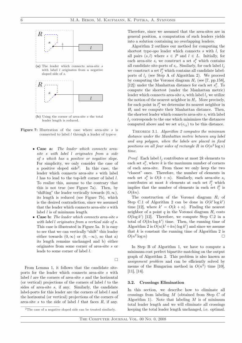
Figure 7: Illustration of the case where area-site s isconnected to label l through a leader of type-o

• Case a: The leader which connects area-site s with label l originates from a sideof s which has a positive or negative slope.For simplicity, we only consider the case ofa positive sloped side2. In this case, theleader which connects area-site s with labell has to lead to the top-left corner of label l.To realize this, assume to the contrary thatthis is not true (see Figure 7a). Then, by“shifting” the leader vertically towards (0,∞),its length is reduced (see Figure 7b), whichis the desired contradiction, since we assumedthat the leader which connects area-site s withlabel l is of minimum length.

• Case b: The leader which connects area-site swith label l originates from a vertical side of s.This case is illustrated in Figure 5a. It is easyto see that we can vertically “shift” this leadereither towards (0,∞) or (0,−∞), so that a)its length remains unchanged and b) eitheroriginates from some corner of area-site s orleads to some corner of label l.

From Lemma 1, it follows that the candidate site-ports for the leader which connects area-site s withlabel l are the corners of area-site s and the horizontal(or vertical) projections of the corners of label l to thesides of area-site s, if any. Similarly, the candidatelabel-ports for this leader are the corners of label l andthe horizontal (or vertical) projections of the corners ofarea-site s to the side of label l that faces R, if any.

2The case of a negative sloped side can be treated similarly.

Therefore, since we assumed that the area-sites are ingeneral position, a computation of such leaders yieldsinto a solution containing no overlapping leaders.

Algorithm 2 outlines our method for computing theshortest type-opo leader which connects s with l, forall pairs (s, l) where s ∈ P and l ∈ L. Initially, foreach area-site si we construct a set sp

i which containsall candidate site-ports of si. Similarly, for each label ljwe construct a set lpj which contains all candidate label-ports of lj (see Step A of Algorithm 2). We proceedby computing the Voronoi diagram Hi (see [7, pp.158],[12]) under the Manhattan distance for each set sp

i . Tocompute the shortest (under the Manhattan metric)leader which connects area-site si with label lj we utilizethe notion of the nearest neighbor in Hi. More precisely,for each point in lpj we determine its nearest neighbor inHi and we compute their Manhattan distance. Then,the shortest leader which connects area-site si with labellj corresponds to the one which minimizes the distancescomputed above and we set w(eij) to be this distance.

Theorem 3.1. Algorithm 2 computes the minimumdistance under the Manhattan metric between any labeland any polygon, when the labels are placed in fixedpositions on all four sides of rectangle R in O(n2 log n)time.

Proof. Each label lj contributes at most 2k elements toeach set sp

i , where k is the maximum number of cornersof each area-site. From those we only keep the two“closest” ones. Therefore, the number of elements ineach set sp

i is O(k + n). Similarly, each area-site si

contributes at most k elements at each set lpj whichimplies that the number of elements in each set lpi isO(kn).

The construction of the Voronoi diagram Hi ofStep C.1 of Algorithm 2 can be done in O(k′ log k′)time [12], where k′ = O(k + n). Finding the nearestneighbor of a point q in the Voronoi diagram Hi costsO(log k′) [12]. Therefore, we compute Step C.2 in atotal of O(kn log k′) time. Then, the running time ofAlgorithm 2 is O(n(k′+kn) log k′) and since we assumethat k is constant the running time of Algorithm 2 isO(n2 log n)

In Step B of Algorithm 1, we have to compute aminimum-cost perfect bipartite matching on the outputgraph of Algorithm 2. This problem is also known asassignment problem and can be efficiently solved bymeans of the Hungarian method in O(n3) time [10],[11], [14].

3.2. Crossings Elimination

In this section, we describe how to eliminate allcrossings from labeling M (obtained from Step C ofAlgorithm 1). Note that labeling M is of minimumtotal leader length and we will eliminate all crossingskeeping the total leader length unchanged, i.e. optimal.



Algorithm 2: Shortest Leader Computation.input : A set P = {s1, . . . , sn} of n gc-polygons

on the plane and a set L = {l1, . . . , ln} ofn uniform labels placed on the boundaryof R.

output: A complete weighted bipartite graphG = (P ∪ L,E,w) between all area-sitessi ∈ P and all labels lj ∈ L, where theweight w(eij) of edge eij = (si, lj) ∈ E isthe length of the shortest (under theManhattan metric) leader, which connectssi with lj .

Step A: Initiate output graph.Construct a graph G = (P ∪ L,E,w) between allarea-sites si ∈ P and all labels lj ∈ L, where theweight w(eij) of an edge eij = (si, lj) ∈ E isinitially equal to zero.

Step B: Determine all possible site and label-ports.for each area-site si (1 ≤ i ≤ n) doAdd the corners of si to sp

i .for each label lj (1 ≤ j ≤ n) doif (lj is located to the right or left side of R)thenFind the intersection points of each edge ofsi with the horizontal lines passing from eachcorner of label lj that faces R and in eachcase select the closest one.

elseFind the intersection points of each edge ofsi with the vertical lines passing from eachcorner of label lj that faces R and in eachcase select the closest one.

Add these points to spi .

for each label lj (1 ≤ j ≤ n) doAdd the corners of lj to lpj .for each area-site si (1 ≤ i ≤ n) doFind the intersection points of the edge of ljthat faces R with the perpendicular to it linespassing from each corner of area-site si. Addthese points to lpj .

Step C: Shortest leader computation.for each area-site si (1 ≤ i ≤ n) do1. Construct the Voronoi diagram Hi (under the

Manhattan distance) for spi .

2. for each element of lpj doFind the nearest neighbor in Hi and computetheir Manhattan distance. Set w(eij) to be theminimum such distance.

Lemma 2. Let M be an opo-labeling (which mightcontain crossings) obtained from Step C of Algorithm 1.Let ci and cj be a pair of intersecting leaders originating

R

si

sjcj

ci

(a) Before rerouting.

R

si

sjc′

j

c′

i

(b) After rerouting.

Figure 8: A pair of intersecting leaders ci and cj .

from area-sites si and sj, respectively. Then, thefollowing hold:

i) The labels li and lj of these leaders lie on twoadjacent sides of the enclosing rectangle R. Let Abe their incident corner.

ii) Leader ci and cj are oriented towards corner A ofthe enclosing rectangle R.

iii) Leaders ci and cj can be rerouted so that they donot cross each other and the sum of their leaderlength remains unchanged.

Proof.

Proof of statement (i): To prove statement (i), weshow that labels li and lj can not both lie on the sameor opposite sides of R. For the sake of contradiction,assume first that the labels li and lj lie on the sameside, say the right side, and the leaders ci and cj

intersect. Then the intersection takes place outsiderectangle R (in the track routing area; see Figure 8a).By swapping the labels to which each area-site isconnected, we can reduce the total leader lengthand also eliminate the crossing (see Figure 8b), acontradiction since we assumed that the total leaderlength of the labeling is minimum.We now consider the case where the labels li andlj lie on opposite sides of rectangle R. Then, sincethe leaders intersect each other, the segments of theleaders which are inside the rectangle (and incidentto the area-sites) have to intersect. However, sincethese segments are parallel to each other, they haveto overlap. Again, by swapping the labels to whicheach area-site is connected, we can reduce the totalleader length (and also eliminate the overlapping), acontradiction since we assumed that the total leaderlength of the labeling is minimum (see an example inFigure 9).



Rsi

sj

cj

ci


Rsi

sj

c′

j

c′

i


Figure 9: A pair of overlapping leaders ci and cj .

Proof of statement (ii): Let A be the corner whichis incident to the two sides of the rectangle Rcontaining the labels associated with leaders ci andcj . In order to show that in a labeling of minimumtotal leader length both leaders ci and cj are orientedtowards corner A, it is enough to show that (ina labeling of minimum total leader length) it isimpossible to have one or both leaders oriented awayof corner A. We proceed to consider these two cases:

Case (a): Exactly one leader, say cj, is orientedaway of corner A. This case is described in the leftpart of Figure 10a. Rerouting both leaders ci and cj

as in Figure 10a results in a reduction of the totalleader length, a contradiction since we assumed thatthe total leader length of the labeling is minimum.Case (b): Both leaders ci and cj are oriented awayof corner A. This case is described in the left partof Figure 10b. When both leaders are oriented awayof corner A, rerouting both leader ci and cj results inhigher reduction of the total leader length (comparedto Case (a) where only one leader was oriented awayof corner A). The rerouting of the leaders is depictedin Figure 10b.

Having eliminated cases (a) and (b), where one orboth crossing leaders are oriented away of corner A,the only case left is the one where both leaders ci

and cj are oriented towards corner A. Such a case isdepicted in Figure 10c.

Proof of statement (iii) : In order to show thatleaders ci and cj can be rerouted so that they do notcross each other and the sum of their leader lengthsremains unchanged, we partition the first segment ofeach leader ci and cj into two sub-segments from theircrossing point to the sides of the enclosing rectange

(see Figure 10c). Then, obtain the new leaders c′i andc′j by a sliding the (sub)segments of leaders ci and cj ,leaving their sum unchanged.

In the following, we show that given a labelingof minimum total leader length which may containcrossings of those described in Lemma 2, we canefficiently resolve all crossings yielding to a newcrossing free labeling so that the total leader length isunchanged.

Theorem 3.2. Let M be an opo-labeling (whichmight contain crossings) obtained from Step C ofAlgorithm 1. We can always identify a crossing-freeopo-labeling M ′ with total leader length equal to that ofM (step D of Algorithm 1). Moreover, labeling M ′ canbe obtained in O(n log n) time.

Proof. We show how to eliminate all crossings oflabeling M by rerouting the crossing leaders. Ourmethod performs two passes over the area-sites, one inthe left-to-right and one in the right-to-left direction.

Consider first the left-to-right pass. In the left-to-right pass of labeling M , we consider all area-siteswith labels on the right side of the rectangle. Weexamine the area-sites from left-to-right and we areinterested only on those who have crossing leaders.Let si be the leftmost3 such area-site and let ci bethe leader that connects it with its correspondinglabel on the right side of the rectangle (see the leftdrawing of Figure 11). Lemma 2.i implies that leaderci intersects only with leaders that are connected withlabels either on the top or bottom side of rectangle R.Without loss of generality, assume that ci is orientedtowards the bottom-right corner of the rectangle, sayA. Then all leaders that intersect ci have their labelson the bottom side of R and are also oriented towardsA (by Lemma 2.ii). Let ck be the leftmost leaderthat intersects ci, and let sk be its incident area-site.According to Lemma 2.ii, we can reroute leaders ci andck so that the total leader length remains unchanged(see the right drawing of Figure 11). Note that thererouting possibly eliminates more than one crossingbut, in general, it might also introduce new crossings.However, the total number of crossings is reduced4 and,more importantly, the leftmost area-site incident to anintersecting leader connected to a label on the rightside of the rectangle is located to the right of area-sitesi. Continuing in the same manner, the leftmost area-site which participates in a crossing (in the left-to-rightpass) is pushed to the right, which guarantees that all“left-to-right” crossings are eventually eliminated.

3Note that the sorting of the area-sites is based on thecoordinates of their ports.

4This is because the new area that contains the area-sites withleaders that cross c′k (refer to the gray colored rectangle of theright part of Figure 11) is fully contained in the area containingthe area-sites with leaders intersecting ci (refer to the gray coloredrectangle of the left part of Figure 11).



sj

R si

cj

ci reroute(ci,cj)

R si

c′

j

c′

i

sj

A

(a) Leader ci (cj) is oriented towards (away of) corner A.

sj

R si

cj

ci reroute(ci,cj)

R si

c′

j

c′

i

sj

AA

(b) Both leaders ci and cj are oriented away of corner A.

sj

R si

cj

ci reroute(ci,cj) sj

R si

c′

j

c′

i

AA

(c) Both leaders ci and cj are oriented towards corner A.

Figure 10: Rerouting used to prove that in an opo-labeling of minimum total leader length, two crossing leaders are orientedtowards the corner incident to the sides of the rectangle containing the associated labels and that their crossingcan be eliminated without reducing the sum of their leader length.

R

sici

reroute(ci,ck)sk

ck

R

si

c′

ksk

c′

i

AA

Figure 11: Rerouting the crossing leaders ci and ck, the leftmost area-site incident to an intersecting leader connected to alabel on the right side of the rectangle is located to the right of area-site si.

Also note that it is impossible to introduce new“right-to-left” crossings, when the left-to-right pass isexecuted. To see this, assume that such a crossing wasintroduced and that it involves leader ci and the leaderc which connects a area-site s to a label on the left sideof the rectangle (see Figure 12). By Lemma 2.i bothleaders c′i and c′ must be oriented towards corner B, acontradiction since leader c′i is oriented away of cornerB (and towards corner A).

From the above discussion, it follows that a left-to-right pass eliminating crossings involving leaderswith their associated labels on the right side of therectangle, followed by a similar right-to-left pass, resultsto a labeling M ′ without any crossings and of totalleader length equal to that of M , that is, minimum.Additionally, since we always keep the position of bothsite and label-ports unchanged the implied labeling willnot contain overlapping leaders. This follows from



R

si

c′

ksk

c′

i

sc

ci

ck

AB

reroute(ci,ck)

R

si

c′

ksk

c′

i

sc

ci

ck

AB

Figure 12: We can not introduce any “right-to-left” crossing during the left-to-right pass.

Lemma 1 and the assumption that the area-sites arein general position.

To complete the proof of the theorem, it remainsto explain how to obtain in O(n log n) time the newlabeling M ′, given labeling M of minimum total leaderlength. Consider the left-to-right pass. The analysisfor the right-to-left pass is similar. During the pass, weprocess the area-sites with labels on the right side of theenclosing rectangle in order of increasing x-coordinate.Sorting the area-sites in increasing order with respectto the x-coordinate of their corresponding site-ports canbe done in O(n log n) time.

In order to process a new area-site si and to eliminatethe crossings involving its leader ci, we have to identifythe leftmost area-site sk such that its correspondingleader ck intersects leader ci. Of course, the intersectioninvolves the first o-segment of leader ci. Without loss ofgenerality, assume that leader ci is oriented towards thebottom-right corner of the enclosing rectangle. The casewhere it is oriented towards the top-right corner can betreated similarly. Then, according to Lemma 2.ii allleaders intersecting leader ci are also oriented towardsthe bottom-right corner and, thus, their associatedlabels are placed on the bottom side of the enclosingrectangle. So, leader ci can only intersect vertical linesegments which have one of their end-points on thebottom side of the enclosing rectangle. This impliesthat we can relax the restriction that these segmentsare of finite size and assume that they are semi-infiniterays having their associated site-ports as their highestendpoints. This is due to the fact that all leaderintersections take place inside the enclosing rectangle.

Under this assumption, the processing of the area-sites during the left-to-right pass can be accomplishedby employing a data structure supporting queries ofthe form “given a set of points Q that change underinsertions and deletions, a threshold value y0 and aquery range (l, r), return the point of Q with thesmallest x-coordinate that is located within the rectangle(l, r) × (y0, tR)5”. The MinXInRectangle query6 just

5Recall that tR denotes the y-coordinate of the top-rightcorner of the enclosing rectangle R

6In Figure 12, the MinXInRectangle query corresponds todetermining the leftmost leader which is contained within thegray colored rectangle.

described can be answered in time O(log n) time byemploying a dynamic priority search tree based onhalf-balanced trees [13, pp 209]. The insert (forinitialization) and delete operations cost O(log n) time.This results to a total of O(n log n) time for the left-to-right pass and, consequently, for the elimination of allcrossings.

Theorem 3.3. Given a site set P of n gc-polygonsand a label set L of n uniform size labels placed atfixed positions on the boundary of R, we can compute inO(n3) time a legal opo-labeling of minimum total leaderlength.

Proof. In Step A of Algorithm 1, we construct acomplete weighted bipartite graph G = (P ∪ L,E, w)between all area-sites si ∈ P and all labels lj ∈ L. Eachedge (si, lj) ∈ E of G is assigned a weight dij equalto the Manhattan length of the shortest (under theManhattan metric) leader, which connects area-site si

with label lj . According to Theorem 3.1, this step costsO(n2 log n) time, assuming that the maximum numberof corners of a type gc-polygon site is fixed.

In Step B of Algorithm 1, we have to computea minimum cost bipartite matching on the outputgraph of Algorithm 1. As already mentioned this willcost O(n3) time. The solution obtained from Step Cof Algorithm 1 might contain crossing leaders. InStep D of Algorithm 1, the crossings are eliminated inO(n log n) time. Thus, the total time complexity ofAlgorithm 1 is O(n3).

3.3. Sample Labeling of type-opo Leaders

Figures 13 and 14 depict the regions of Germany. Inboth Figures, the labels are placed on two opposite sidesof R and the leaders are of type opo. In Figure 13 apoint is arbitrarily selected as the representative of eachregion. The labeling of Figure 13 is visually improvedin Figure 14 by replacing these points with rectangleswithin each region. Both labelings are optimal in termsof total leader length. However, the total leader lengthof Figure 14 is reduced by 37% compare to that ofFigure 13. Note that we also achieved to reduce thenumber of leader bends to 5 (in Figure 14) from 8 (in



Figure 13: A regional map of Germany; a point is therepresentative of each region.

Figure 14: A visually improved map; a rectangle is therepresentative of each region.

Figure 13), just by the use of rectangular area-sitesinstead of point-sites.

4. TWO-SIDE LABELING OFGC-POLYGONS WITH TYPE-POLEADERS

In this section, we consider the problem of labeling area-sites represented as gc-polygons with leaders of type-po. We further assume that we have uniform size labelswith sliding label-ports, placed on two opposite sides ofthe enclosing rectangle R. Our objective is to determinea legal boundary labeling so that the total leader lengthis minimized.

To deal with this problem, we use the (matchingbased) Algorithm 1 for the case of type-opo leaders toget a labeling of minimum total leader length. Thiscan be done in O(n3) time. We proceed by replacingthe type-opo leaders with type-po leaders. Note thatconnecting a site to its label with a type-opo or a type-po leader requires leaders of the same length under theManhattan metric, assuming that we keep the positionof both site and label-ports unchanged. Therefore,

sj

R si

cj

ci


sj

R si

c′

j

c′

i


Figure 15: The rerouting of two crossing po-leaders doesnot always eliminate their crossing.

the solution obtained in this manner remains optimalin terms of total leader length, but it might containcrossings.

Possible crossings between leaders to the same sideof the enclosing rectangle are resolved following asimilar strategy as in [4], without changing the totalleader length. This can be done in O(n2) additionaltime [4, pp.229]. Moreover, we can easily observe thatcrossings between leaders that go to opposite sides ofthe enclosing rectangle cannot occur. This is due tothe fact that swapping these crossing leaders wouldresult in a solution with smaller total leader length, acontradiction since we assume that the original solutionminimizes the total leader length. Note that the samestrategy can be applied in the case where the labels canbe placed on only one side of the enclosing rectangle R.The following theorem summarizes our result.

Theorem 4.1. Given a site set P of n gc-polygonsand a label set L of n uniform size labels placed atfixed positions along two opposite sides of R, we cancompute in O(n3) time a legal po-labeling of minimumtotal leader length.

For the case where the labels can occupy two adjacentsides of the enclosing rectangle R, there exists instancesof the problem where it is not feasible to determinea crossing-free type-po labeling, irrespectable of thelabeling optimization criteria. This follows from theobservation that the rerouting of two crossing po-leadersdoes not always eliminate their crossing (see Figure 15).Figure 16 illustrates an instance of the problem wherethe labels occupy all four sides of R. All sites are



Figure 16: An instance which admits no crossing-freelabeling.

contained within the gray colored rectangular area thatis formed from i) the top left corner of the enclosingrectangle R and ii) the intersection of the lines thatcoincide with the bottom side of the topmost label onthe left side of R and the right side of the leftmostlabel on the top side of R. Since two sites have to beconnected to the dark-gray colored labels (incident tothe bottom-right corner of R), a crossing as the one ofFigure 15 will inevitably arise, which implies that thisinstance admits no-crossing free solution. The followingtheorem summarizes this result.

Theorem 4.2. Consider the area-feature boundarylabeling problem with type-po leaders, uniform labelsplaced at fixed positions. If labels occupy two adjacentsides of the enclosing rectangle there exists instancesthat admit no legal (i.e. crossing-free) labelingirrespectable of the labeling optimization criteria.

4.1. Sample Labeling of type-po Leaders

Figures 17 and 18 depict the regions of France. In bothFigures, the labels are restricted on one side of R andthe leaders are of type po. In Figure 17 a point isarbitrarily selected as the representative of each region.The labeling of Figure 17 is visually improved in Figure18 by replacing these points with rectangles within eachregion. Both labelings are optimal in terms of totalleader length. However, the total leader length of Figure18 is reduced by 10.73% compared to that of Figure 17.Note that the order of the labels is nearly the sameas the order of their corresponding sites in Figure 18,in contrast to Figure 17. We also achieved to reducethe number of leader bends to 1 (in Figure 18) from 14(in Figure 17), just by the use of rectangular area-sitesinstead of points.

Figure 17: A regional map of France; a point is therepresentative of each region.

Figure 18: A visually improved map; a rectangle is therepresentative of each region.

5. CONCLUSIONS

In this paper, we considered the area-feature boundarylabeling problem where area-sites are presented as gc-polygons instead of points. We presented an efficientalgorithm to determine opo-labelings of minimum totalleader length, where the labels are of uniform size,with sliding label-ports, placed on all four sides of theenclosing rectangle R. For the special case, where thelabels can placed on two opposite sides of the enclosingrectangle R, we extended this algorithm to support po-leaders.

It is intuitive that the quality of the labelings can beimproved by allowing combinations of different types ofleaders. To the best of our knowledge no algorithmsexist for this model in the map labeling literature.

All known type-opo boundary labelings use a trackrouting area outside the enclosing rectangle to route thep-segment of the leader. Routing the p-segment insidethe enclosing rectangle might lead to visually improvedlabelings.

The evaluation of different optimization criteria (e.g.the one of minimizing the total number of leader bends)



would also be of particular interest. Furthermore, noresults were presented for the cases of sliding labels ornon-uniform labels. For the latter problem very fewresults exists in boundary labeling, in general.

Another line of research would be to try to findefficient ways of determining for each region of a mapa representative gc-polygon that has less than kcorners, where k is a constant.

REFERENCES

[1] M. A. Bekos, M. Kaufmann, K. Potika, andA. Symvonis. Multi-stack boundary labeling problems.In S. Arun-Kumar and N. Garg, editors, Proc. 26thConference on Foundations of Software Technology andTheoretical Computer Science (FSTTCS2006), LNCS4337, pages 81–92, 2006.

[2] M. A. Bekos, M. Kaufmann, K. Potika, andA. Symvonis. Polygons labelling of minimum leaderlength. In M. Kazuo, S. Kozo, and T. Jiro,editors, Proc. Asia Pacific Symposium on InformationVisualisation (APVIS2006), CRPIT 60, pages 15–21,2006.

[3] M. A. Bekos, M. Kaufmann, and A. Symvonis. Label-ing collinear sites. In Proc. Asia Pacific Symposium onInformation Visualisation (APVIS2007), IEEE, pages45–51, 2007.

[4] M. A. Bekos, M. Kaufmann, A. Symvonis, and A. Wolff.Boundary labeling: Models and efficient algorithms forrectangular maps. Computational Geometry: Theoryand Applications, 36:215–236, 2007.

[5] M. Benkert, H. Haverkort, M. Kroll, and M. Nöllen-burg. Fast algorithms for one-sided boundary label-ing. In Proc. 15th Int. Symposium on Graph Drawing(GD’07). To appear.

[6] M. Benkert and M. Nöllenburg. Improved algorithmsfor length-minimal one-sided boundary labeling. InProc. 23rd European Workshop on ComputationalGeometry (EWCG’07), pages 190–193, 2007.

[7] M. de Berg, M. van Kreveld, M. Overmars, andO. Schwarzkopf. Computational Geometry: Algorithmsand Applications. Springer-Verlag, second edition,2000.

[8] M. Formann and F. Wagner. A packing problem withapplications to lettering of maps. In Proc. 7th Annu.ACM Sympos. Comput. Geom., pages 281–288, 1991.

[9] H.-J. Kao, C.-C. Lin, and H.-C. Yen. Many-to-oneboundary labeling. In Proc. Asia Pacific Symposium onInformation Visualisation (APVIS2007), IEEE, pages65–72, 2007.

[10] H. W. Kuhn. The Hungarian method for the assign-ment problem. Naval Research Logistic Quarterly,2:83–97, 1955.

[11] E. Lawler. Combinatorial Optimization: Networks andMatroids. Holt, Rinehart & Winston, New York, 1976.

[12] D. T. Lee. Two-dimensional voronoi diagrams in thelp-metric. J. ACM, 27(4):604–618, 1980.

[13] K. Mehlhorn. Data structures and algorithms 3: multi-dimensional searching and computational geometry.Springer-Verlag New York, Inc., New York, NY, USA,1984.

[14] C. H. Papadimitriou and K. Steiglitz. CombinatorialOptimization : Algorithms and Complexity. DoverPublications, 1998.

[15] A. Wolff and T. Strijk. The Map-LabelingBibliography. http://i11www.ira.uka.de/map-labeling/bibliography. , 1996.


Area-Feature Boundary Labeling (1)

Documents

Transcript of Area-Feature Boundary Labeling (1)