Automatic labeling of molecular biomarkers of ...

RESEARCH ARTICLE

Automatic labeling of molecular biomarkers

of immunohistochemistry images using fully

convolutional networks

Fahime Sheikhzadeh1,2*, Rabab K. Ward1, Dirk van Niekerk3, Martial Guillaud2

1 Department of Electrical Engineering, University of British Columbia, Vancouver, British Columbia, Canada,

2 Department of Integrated Oncology, Imaging Unit, British Columbia Cancer Research Centre, Vancouver,

British Columbia, Canada, 3 Department of Pathology, British Columbia Cancer Agency, Vancouver, British

Columbia, Canada

* [email protected]

Abstract

This paper addresses the problem of quantifying biomarkers in multi-stained tissues based

on the color and spatial information of microscopy images of the tissue. A deep learning-

based method that can automatically localize and quantify the regions expressing bio-

marker(s) in any selected area on a whole slide image is proposed. The deep learning net-

work, which we refer to as Whole Image (WI)-Net, is a fully convolutional network whose

input is the true RGB color image of a tissue and output is a map showing the locations of

each biomarker. The WI-Net relies on a different network, Nuclei (N)-Net, which is a convo-

lutional neural network that classifies each nucleus separately according to the biomarker(s)

it expresses. In this study, images of immunohistochemistry (IHC)-stained slides were col-

lected and used. Images of nuclei (4679 RGB images) were manually labeled based on the

expressing biomarkers in each nucleus (as p16 positive, Ki-67 positive, p16 and Ki-67 posi-

tive, p16 and Ki-67 negative). The labeled nuclei images were used to train the N-Net

(obtaining an accuracy of 92% in a test set). The trained N-Net was then extended to WI-Net

that generated a map of all biomarkers in any selected sub-image of the whole slide image

acquired by the scanner (instead of classifying every nucleus image). The results of our

method compare well with the manual labeling by humans (average F-score of 0.96). In

addition, we carried a layer-based immunohistochemical analysis of cervical epithelium,

and showed that our method can be used by pathologists to differentiate between different

grades of cervical intraepithelial neoplasia by quantitatively assessing the percentage of

proliferating cells in the different layers of HPV positive lesions.

Introduction

This study addresses the automation of Immunohistochemistry (IHC) image analysis in quan-

titative pathology. IHC staining is a tissue-based biomarker imaging technology widely used to

identify and visualize target cellular antigens specific to certain tissues. In the process, a fixed

PLOS ONE | https://doi.org/10.1371/journal.pone.0190783 January 19, 2018 1 / 18

a1111111111

a1111111111

a1111111111

a1111111111

a1111111111

OPENACCESS

Citation: Sheikhzadeh F, Ward RK, van Niekerk D,

Guillaud M (2018) Automatic labeling of molecular

biomarkers of immunohistochemistry images

using fully convolutional networks. PLoS ONE 13

(1): e0190783. https://doi.org/10.1371/journal.

pone.0190783

Editor: Christophe Egles, Universite de Technologie

de Compiegne, FRANCE

Received: June 28, 2017

Accepted: December 20, 2017

Published: January 19, 2018

Copyright: © 2018 Sheikhzadeh et al. This is an

open access article distributed under the terms of

the Creative Commons Attribution License, which

permits unrestricted use, distribution, and

reproduction in any medium, provided the original

author and source are credited.

Data Availability Statement: All relevant data are

available from Open Science Framework: https://

osf.io/c74wu/ (Identifiers: DOI 10.17605/OSF.IO/

C74WU, ARK c7605/osf.io/c74wu).

Funding: This work was funded through a Natural

Sciences and Engineering Research Council of

Canada grant (RGPIN 2014-04462) to RKW and a

National Institute of Health funded program project

grant (P01–CA-82710). The funders had no role in

study design, data collection and analysis, decision

to publish, or preparation of the manuscript.

https://doi.org/10.1371/journal.pone.0190783

http://crossmark.crossref.org/dialog/?doi=10.1371/journal.pone.0190783&domain=pdf&date_stamp=2018-01-19








http://creativecommons.org/licenses/by/4.0/

https://osf.io/c74wu/

https://osf.io/c74wu/

https://doi.org/10.17605/OSF.IO/C74WU

https://doi.org/10.17605/OSF.IO/C74WU

tissue sample is first sectioned and mounted on a slide, then stained with different IHC bio-

markers, and finally imaged by a scanner or a charge-coupled device color camera mounted

on an optical microscope. Immunohistochemistry imaging is commonly used in the detection

of specific cell types or cells in specific functional states, which can ultimately reflect the physi-

ological state and the changes in a disease process. Analysis of IHC images can determine the

spatial distribution of every biomarker with respect to the tissue’s histological structures as

well as the spatial relationships amongst the cells expressing each biomarker. This information

could provide valuable insights to the molecular complexity of disease processes, enable new

cancer screening and diagnosis tools, inform the design of new treatments, monitor treatment

effectiveness, and predict the patient response to a treatment. However, the manual quantifica-

tion and localization of the different subsets of cells containing a biomarker (in each IHC-

stained tissue) demands a large amount of time and effort. In addition, qualitative or semi-

quantitative scoring systems suffer from low reproducibility, accuracy, and sensitivity, and

decreased ability to distinguish the different stains apart when they overlap spatially. There-

fore, there is a need for methods that can automatically quantify IHC images. This is, however,

a challenging problem due to the variations caused by the different staining and tissue process-

ing procedures.

The techniques proposed in the literature for quantifying histopathology images are gener-

ally based on traditional image processing approaches that rely on extracting pre-defined fea-

tures of nuclei or cell appearance [1,2]. Using pre-defined features in IHC image analysis

however, raises the concern of low reproducibility and lack of robustness, due to variations in

the nuclei and cell appearance that are caused by the different staining and tissue processing

procedures used by different laboratories. Recently, several studies have shown that deep

learning algorithms such as those employing convolutional neural networks [3], could be used

in histopathology image analysis with great success [4–10]. For example, Jain et al. [4] applied

a convolutional network to segment electron microscopic images into intracellular and inter-

cellular spaces. Ciresan et al. [5] and Wang et al. [9] employed deep learning to respectively

detect mitoses and metastastic breast cancer through quantitative analysis of breast histopa-

thology images. This approach has outperformed other methods by a significant margin [5,9].

Janowczyk et al. [10] demonstrated that the performance of their convolutional approach in

segmentation (nuclei, epithelium, tubule, and invasive ductal carcinoma), detection (lympho-

cyte and mitosis) and classification (lymphoma subtype) applications, was comparable or

superior to existing approaches or human performance.

In this paper, we address the automation of IHC image analysis in quantitative pathology.

We propose a deep learning method to detect and locate two biomarkers present in a cervical

intra-epithelial lesion and quantify the percentage of proliferating cells in different layers of a

p16 positive epithelium. The tissue could be a normal cervix tissue, low-grade Cervical Intrae-

pithelial Neoplasia (CIN), or high-grade CIN. The proposed deep learning network is a fully

convolutional neural network that can take an IHC image as an input, and detect and locate

the different biomarkers presented in all cells of the image. This network is an extension of a

convolutional neural network that is trained by using RGB images of nuclei, to classify a

nucleus according to its expressed biomarker.

The benefit of using the deep learning approach (over image processing methods that rely

on capturing pre-defined features of nuclei or cell appearance) is that the feature descriptors

are automatically learned in the convolution kernels [11] (during the training of the network).

Therefore, there is no need to find and quantify sophisticated features for every group of cells

expressing a specific biomarker. We believe that by eliminating the need to find and quantify

advanced features for each cell expressing a biomarker, we could develop more reproducible

methods for biomarker localization in IHC images. In addition, in our proposed approach,

Quantitative IHC analysis


Competing interests: The authors have declared

that no competing interests exist.


there is no need for pre-processing the RGB images before feeding them to the network. This

is in contrast to most methods in the literature, as these methods rely on complicated process-

ing like un-mixing techniques (e.g. un-mixing multi-spectral images and color un-mixing in

RGB images).

We should keep in mind that there is a drawback in employing deep neural networks. They

performed very well and won grand challenges across different practical areas [11,12], and of

course in the field of medical imaging [5], but the good performance of deep neural networks

comes at a cost; the need for large data sets, computational complexity, and being black

box predictors which can make their performances unpredictable.

In this paper, first we explain how we have collected our dataset which is composed of IHC

images selected on whole slide images of cervical biopsies. Then we discuss the methods we

have used to detect and localize the different biomarkers in these images. After that, we explain

the experimental design, results and validation metrics we have used to evaluate our proposed

approach.

Dataset

Patient recruitment and specimen collection

The uterine cervical biopsy specimens we used were obtained from baseline patient visits for

colposcopy review at the Women’s Clinic at Vancouver General Hospital, as described in

Sheikhzadeh et al. [13]. The samples were collected during a clinical trial over a period of 22

months (April 2013- February 2015). The study presented in this paper was part of that clinical

trial. All patients had given informed consent, and the study was approved by the UBC BCCA

Research Ethics Board and the Vancouver Coastal Health Research Institute (Protocols H09-

03303 and H03-61235). These patients had been referred to the clinic based on prior abnormal

Pap smear test results. All patients were later diagnosed as having low-grade CIN, high-grade

CIN, or no abnormality (normal cervix). The uterine cervix biopsies, both normal and abnor-

mal, were collected by trained gynecologists (DM, TE) from clinically selected sites. Biopsy

specimens were immediately placed in saline after they were collected, and then transferred to

the hospital pathology lab in formalin fixative. Eventually, biopsy samples were embedded in

paraffin, and nine 4-μm transverse sections were cut from each of them and mounted on slides

[13].

Staining and imaging specimens

For this study, we used 4 out of the 9 slides cut from each biopsy. The other slides were used

for other projects. Out of the nine slides cut from each biopsy, three slides were stained with

Hematoxylin and Eosin (H&E) and reviewed by an expert pathologist (DVN) to establish dis-

ease grade as either: normal, reactive atypia, CIN1, CIN2, and CIN3. A fourth slide was double

immunostained for p16/Ki-67, using the CINtec PLUS kit (Roche mtm laboratories, Mann-

heim, Germany) according to the manufacturer’s instruction, and then counterstained with

Hematoxylin. This slide was used for immunohistochemical analysis. Our study included 69

slides in total. We randomly selected slides from biopsies with different disease grade to make

sure our dataset includes all disease grades. To ensure that our analysis was not biased by our

staining or tissue processing procedure, the slides were randomly assigned to one of two

pathology cyto-technicians. The slides were split into seven batches (six batches of 10 slides

and one batch of 9 slides). One of the two cyto-technicians stained three batches and the other

technician stained four batches; one batch per week. For all the slides, one reagent lot was used

and the staining was performed manually.




Each immunostained tissue sample (IHC slide) contained three labels: 1) a counterstain

that labeled every nucleus (Hematoxylin [H]), 2) a chromogen (fast red) that labeled a

nucleus-bound IHC biomarker (Ki-67 antigen), and 3) a chromogen (DAB) that enabled the

visualization of the other IHC biomarker (p16 antigen), which is localized in the nuclei and

cytoplasm [14]. The Ki-67 antigen is one of the most commonly used markers of cell prolifera-

tion, and is routinely applied to biopsies of cancerous or pre-cancerous cervical tissues [15].

The p16 protein is an important tumor suppressor protein that regulates the cell cycle, and is

also commonly used as a diagnostic biomarker of cervical neoplasia [16].

We scanned each of the obtained IHC slides with a Pannoramic MIDI whole slide scanner

(3DHISTECH Ltd., Budapest, Hungary) at 20X magnification. Using Pannoramic Viewer

(3DHISTECH Ltd.) at 4X magnification we located the regions exhibiting the worst diagnosis

on the H&E slide, and marked the same diagnostic areas on the corresponding CINtec stained

slide. Then, the marked areas were exported to RGB images in TIFF format (with the total

magnification of 80X and the resolution of 96 dpi). A total of 69 images, varying in size from

1024×1024 up to 17408×17408 pixels, were used in our analysis and validation. For simplicity,

we will refer to these images as IHC images in the rest of this paper.

Biomarker labeling method

The biomarker labeling, outlined in Fig 1 was done in two main steps: i) training a convolu-

tional neural network which we will refer to as Nuclei(N)-Net to label the expressed biomark-

ers in one nucleus, and ii) transforming the N-Net to a fully convolutional network to locate

all cells expressing each of the different biomarkers in an IHC image. We will refer to this net-

work as Whole Image (WI)-Net.

In the first step, the nuclei in the IHC images were segmented. The resulting nuclei images

were labeled and then fed as inputs to the N-Net. We would like to clarify that in our

Fig 1. A two-step approach to biomarker labeling in IHC images. Step one (top): N-Net was trained with nucleus images segmented from IHC images in the

training set, where each image had one nucleus only. This network learned to classify each nucleus image according to the expressed biomarker(s) in its respective

nucleus. Step two (bottom): the trained classifier (N-Net) was extended to WI-Net. This end-to-end, pixel-to-pixel network localized biomarkers of the IHC

images. The input to the WI-Net is an IHC image and the output is a heat-map of the two biomarker expression.

https://doi.org/10.1371/journal.pone.0190783.g001





segmentation, we did not aim to delineate the exact border of the nucleus or the cytoplasm

(which was not necessary for our application) and therefore, each nucleus image was repre-

sented by a square image consisting of the nucleus and its surrounding cytoplasm. The outputs

of the N-Net were the labels that identified the expressed biomarker in the nucleus/cytoplasm

of each input image (Fig 1, top). In the second step, a whole IHC image of arbitrary size was

fed into the WI-Net, and for each pixel the probability of each biomarker being expressed was

calculated. These probability values were ultimately used to produce a color heat-map of the

different regions expressing different biomarkers in the IHC image (Fig 1, bottom).

Nuclei classification using N-Net

The N-Net was the classifier we built for labeling the expressed biomarkers in nuclei images.

Fig 2 shows the schematic representation of the N-Net configuration, which is a convolutional

neural network [3] consisting of five layers. The input to the first layer is an RGB image con-

taining one nucleus only. The first layer is a convolution layer that convolves the input image

with K filters, each having a kernel size of F1× F1×3. These kernel matrices are learned by the

N-Net. The second layer is a max-pooling layer with a kernel size of F2 by F2, which is a sub-

sampling layer that reduces the size of the image. The third and forth layers are fully connected

layers, each containing M neurons. The output layer consists of N neurons, each with a Gauss-

ian function. This layer generates labels, showing the probability of each biomarker being pres-

ent in the image.

Biomarker localization in whole slide images using WI-Net

In the previous section, we explained how N-Net was trained as a classifier for images, each

containing one nucleus. In order to employ this classifier for localizing biomarkers on a whole

Fig 2. Schematic representation of the architecture of the N-Net. N-Net consists of one convolution layer, followed by a max-pooling layer and

two fully connected layers. The last layer is the output layer. This network takes an RGB image of a nucleus as input and generates a label as the

output.






IHC image (containing thousands of nuclei), different approaches could be used. For example,

a sliding window (whose size is equal to the N-Net input size) could be employed on each pixel

of the IHC image. Taking the window region as the input of the N-Net and obtaining the

N-Net output, could generate a label for each pixel in the IHC image. The main disadvantage

of this approach is that it could get computationally intensive especially for large input images.

Therefore, we used a more computationally optimized approach in this study, and took advan-

tage of the nature of convolution which could be considered as a sliding window [17]. By

transforming the trained N-Net to WI-Net which is a fully convolutional network, a classifica-

tion map of the IHC image is obtained (rather than generating a single classification of a

nucleus image by the N-Net). This transformation is shown in Fig 3. The fully connected layers

of the N-Net were converted to convolutional layers [17]; this was done for the purpose of

modifying these layers to make them independent of the spatial size.

Experiments and results

Biomarker localization

Preparing nuclei images for training N-Net. To train N-Net, we must first prepare

nuclei images from the whole slide IHC images. To do so, we first selected different regions of

interest (ROI) delineating the basal membrane and the superficial membrane in six whole

slide images and then coarsely segmented the nuclei in each ROI. Fig 4 shows the ROI selec-

tion, the nuclei images and the label corresponding to each of four different protein expres-

sions (p16 positive, Ki-67 positive, p16 and Ki-67 positive, and p16 and Ki-67 negative).

To select the ROIs we used our in-house image analysis software, Getafics [18], and manu-

ally delineated the basal membrane and the superficial membrane within each image. Then,

we detected the nuclei and their centers of gravity within each ROI at magnification of 20X.

This procedure was semi-automated, requiring only minor manual adjustments (described in

[19]).

Digital RGB images, each containing one nucleus, were rescaled to 32 by 32 pixel images

and stored in a gallery. We then manually labeled the nuclei into four groups: i) p16 positive,

ii) Ki-67 positive, iii) both Ki-67 and p16 positive, and iv) both p16 and Ki-67 negative. These

nuclei images along with their group number were considered as the ground truth and used

for training the N-Net.

Fig 3. Schematic representation of the architecture of the WI-Net. The first two layers of WI-Net (convolution and max-pooling layers) are the

same as the first two layers of N-Net illustrated in Fig 2. The last three layers of WI-Net are convolution layers. The input to the WI-Net is a whole IHC

image, and the output is a heat-map of the present biomarker(s) in the IHC image.






We had a total of 4679 labeled nuclei RGB images obtained within the ROIs from the six

IHC images. The IHC images were acquired from six cases: two CIN3, one CIN2, two CIN1

and one negative (normal cervical tissue) cases. Of these 4679 nuclei images, 156 nuclei images

belonging to one of the six IHC images were used for testing the performance of N-Net, and

the remaining 4523 nuclei images obtained from the other five IHC images were used for

training. Table 1 illustrates the distribution of the nuclei in the training and test sets of the dif-

ferent groups.

Training and testing N-Net. We used the following network configuration. As men-

tioned above, the first layer of N-Net was a convolutional layer containing 96 filters with a ker-

nel size of 11×11×3 and stride of 4 through which each filter was slid. The second layer was a

max-pooling layer with a kernel size of 3×3, and stride of 2. In order to define the kernel sizes,

we used a validation set consisting of 161 nuclei images and trained the N-Net with different

kernel sizes. The kernel size corresponding to the lower error rate was selected. The third and

forth layers were fully connected layers, each containing 2048 neurons. The output layer con-

sisted of four neurons. The N-Net was implemented by using the open source, deep learning

framework Caffe [20], and a system with an Intel I5-6600 3.3GHZ Quad core CPU and a

GTX750TI GP.

For training, we used the back-propagation algorithm whereby 4523 labeled nuclei images

were the inputs to the N-Net. The Softmax function was used in the output layer of the N-Net.

We considered four labels (representing the four groups) as the output of the N-Net. The

trained network learned the features corresponding to the presence of following biomarkers in

each nucleus: i) H and p16 (label: 0 0 0 1), ii) H and Ki-67 (label: 0 0 1 0), iii) H and both Ki-67

and p16 (label: 0 1 0 0), iv) H only (absence of Ki-67 and p16) (label: 1 0 0 0). Training was

stopped after 8000 iterations (with an error rate of 0.04 on the training set). Following the

training, we performed the classification on the test set using N-Net. Tables 2 and 3 show the

Fig 4. Sample of nuclei images obtained from an IHC image. ROI (red enclosure) selected in an IHC image, within which the nuclei were segmented in

order to obtain nuclei images for training N-Net (left). Nuclei images expressing different proteins (right); p16 positive, Ki-67 positive, p16 and Ki-67

positive, and p16 and Ki-67 negative.


Table 1. Distribution of nuclei in the training and test sets.

Number of nuclei in the different groups

p16 positive Ki-67 positive Ki-67 & p16 positive p16 and Ki-67 negative Total

Train Set 918 866 1572 1167 4523

Test Set 62 25 52 17 156

https://doi.org/10.1371/journal.pone.0190783.t001






confusion matrix of the results of the training and test sets respectively. According to the con-

fusion matrix, the classification error rate for N-Net was 0.07 on the test set.

To estimate the accuracy of N-Net classification, we also performed a 10-fold cross-valida-

tion analysis. We split the training set (4523 nuclei images) in to 10 subsets (nine sets of 452

nuclei and one set of 455 nuclei). The subsets were approximately balanced in different labels.

We used the same network architecture and training parameters as explained above and

trained the network 10 different times. At each training round, we trained the N-Net by using

9 subsets and then test the network performance on the left out subset. In 10 training rounds,

we obtained the average accuracy of 0.94 (SD = 0.01) on classifying the test subsets. The

obtained accuracy is consistent with the results obtained from training the N-Net with the

train set of 4523 nuclei images and testing its performance on an independent set of 156 nuclei

images. The results suggest that the performance of N-Net is robust to the way we split our

dataset into training and test data.

Labeling biomarkers in IHC images using WI-Net. After training the N-Net in labeling

the expressed biomarker(s) in nuclei image, we transformed the N-Net into WI-Net for ana-

lyzing the whole IHC image. The WI-Net produced a classification map that covers an input

image of arbitrary size (i.e. the produced classification map is not the result of a single classifi-

cation). We transformed the N-Net to WI-Net based on the method presented by Shelhamer

et al [17]. The kernel sizes for WI-Net are the same as N-Net. The only difference is the last

three layers, which are fully connected layer in N-Net and we transfer them to convolutional

layers (with the kernel sizes of 4, 1, and 1 respectively) in WI-Net. Next, we fed each IHC

image as an input to the WI-Net, and obtained a heat-map for each of its biomarker. In total

four heat-maps were produced for each IHC image, each illustrating the regions in the IHC

image that are: i) p16 positive, ii) Ki-67 positive, iii) both p16 and Ki-67 positive, and iv) both

p16 and Ki-67 negative (only expressing H). Fig 5 shows an example of an IHC image (Fig 5a)

and its corresponding heat-map obtained as the output from the WI-Net (Fig 5f).

Visual comparison of the original IHC image and the labeling results from WI-Net (Fig 5a

and 5f) shows that the WI-Net performance in localizing p16 and Ki-67 in the dual-stained

Table 2. Confusion matrix of the classification results on the training set using N-Net.

Training Set

p16 pos. (Predicted) Ki-67 pos. (Predicted) Ki-67 & p16 pos. (Predicted) p16 & Ki-67 neg. (Predicted) Accuracy

p16 pos. (Actual) 869 0 45 4 94.6%

Ki-67 pos. (Actual) 0 835 30 1 96.4%

Ki-67 & p16 pos. (Actual) 79 10 1483 0 94.3%

p16 & Ki-67 neg. (Actual) 1 6 0 1160 99.4%

Overall Accuracy 96.1%


Table 3. Confusion matrix of the classification results on the test set using N-Net.

Test Set

p16 pos. (Predicted) Ki-67 pos. (Predicted) Ki-67 & p16 pos. (Predicted) p16 & Ki-67 neg. (Predicted) Accuracy

p16 pos. (Actual) 59 0 1 2 95.1%

Ki-67 pos. (Actual) 0 25 0 0 100%

Ki-67 & p16 pos. (Actual) 8 0 44 0 84.6%

p16 & Ki-67 neg. (Actual) 0 0 0 17 100%

Overall Accuracy 92.9%







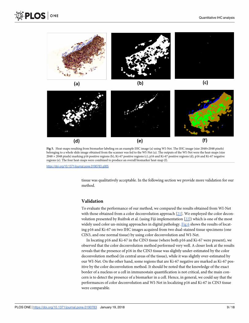
tissue was qualitatively acceptable. In the following section we provide more validation for our

method.

Validation

To evaluate the performance of our method, we compared the results obtained from WI-Net

with those obtained from a color deconvolution approach [21]. We employed the color decon-

volution presented by Ruifrok et al. (using Fiji implementation [22]) which is one of the most

widely used color un-mixing approaches in digital pathology. Fig 6 shows the results of locat-

ing p16 and Ki-67 on two IHC images acquired from two dual-stained tissue specimens (one

CIN3, and one normal tissue) by using color deconvolution and WI-Net.

In locating p16 and Ki-67 in the CIN3 tissue (where both p16 and Ki-67 were present), we

observed that the color deconvolution method performed very well. A closer look at the results

reveals that the presence of p16 in the CIN3 tissue was slightly under-estimated by the color

deconvolution method (in central areas of the tissue), while it was slightly over-estimated by

our WI-Net. On the other hand, some regions that are Ki-67 negative are marked as Ki-67 pos-

itive by the color deconvolution method. It should be noted that the knowledge of the exact

border of a nucleus or a cell in immunostain quantification is not critical, and the main con-

cern is to detect the presence of a biomarker in a cell. Hence, in general, we could say that the

performances of color deconvolution and WI-Net in localizing p16 and Ki-67 in CIN3 tissue

were comparable.

Fig 5. Heat-maps resulting from biomarker labeling on an example IHC image (a) using WI-Net. The IHC image (size 2048×2048 pixels)

belonging to a whole slide image obtained from the scanner was fed to the WI-Net (a). The outputs of the WI-Net were the heat-maps (size

2048 × 2048 pixels) marking p16 positive regions (b), Ki-67 positive regions (c), p16 and Ki-67 positive regions (d), p16 and Ki-67 negative

regions (e). The four heat-maps were combined to produce an overall biomarker heat-map (f).






In the normal tissue (where none of p16 or Ki-67 were present), we observed that our

WI-Net method did not classify any pixel as p16 positive or Ki-67 positive. The color deconvo-

lution method however had mistakenly marked some regions on the tissue as being p16 or Ki-

67-positive. The lack of robustness in the color deconvolution method over different tissue

samples with different disease stages, could be due to difficulty in finding the optimal parame-

ter/threshold setting. It is possible that with a set of parameters the color deconvolution would

perform better in high-grade tissues, but would fail in low-grade tissues.

In addition, we performed two separate analyses in order to evaluate the efficacy of our pro-

posed biomarker labeling method. First, we compared the performance of our fully automatic

algorithm to human performance. Second, we investigated the utility of our immunohisto-

chemical analysis to quantify the proliferation characteristics of the epithelium to aid with

delineating between different pathology grades.

Comparison with manual biomarker labeling. We manually labeled the cells expressing

different biomarkers in IHC images, and then used the labeled cells as the ground truth. Man-

ually obtaining a biomarker heat-map for each IHC image is not easy; it is extremely laborious,

requiring manual delineation of the membrane around each nucleus and cell and labeling each

Fig 6. Comparison between color deconvolution approach and WI-Net approach for locating p16 and Ki-67 positive pixels in two IHC images. The IHC image

on the left two columns corresponds to a high-grade cervical lesion. The IHC image on the right two columns corresponds to a normal cervical epithelium. The first

row shows the RGB images. The second row shows the regions marked as p16 positive by the two methods. The third row shows the regions marked as Ki-67 positive

by the two methods.






pixel in an IHC image. However, the knowledge of the exact border of a nucleus or a cell in

immunostain quantification is not critical, and the main concern is to detect the presence of a

biomarker in a cell. Hence, we only marked the center of the nucleus in each cell and assigned

a label to the center based on the expressing protein(s). To obtain the best possible manual

labeling (in the sense that it could be regarded with confidence as the ground truth for our

comparisons), we asked two experienced cyto-technicians to assign these labels. Basically, the

cyto-technicians worked together and reached to an agreement on the protein expression for

each cell. We considered the label assigned to the center of a nucleus as the ground truth of the

expressed protein(s) in its corresponding cell. We compared this ground truth to the bio-

marker heat-map generated by the outlined proposed method. For each marker, we defined

the following metrics:

• Number of correctly labeled nuclei (true positive): this is the number of nuclei centers in the

ground truth which are marked positive for that biomarker and are classified as positive for

the biomarker heat-map.

• Number of missed nuclei (false negative): this is the number of nuclei centers in the ground

truth which are marked positive for that biomarker and are classified as negative in the bio-

marker heat-map.

• Number of falsely labeled nuclei (false positive): this is the number of nuclei centers in the

ground truth which are not marked positive for that biomarker but are classified as positive

for the biomarker heat-map.

Table 4 shows the validation metrics for the WI-Net performance compared to the human

performance (the ground truth). From the above metrics, we calculate the precision, recall,

and the F-score [23]. We selected two IHC images from our data set and using the proposed

method, we generated their biomarker heat-maps. These images were never seen before by the

network; they were not used (neither as nucleusimages or whole images) for training or testing

the N-Net or WI-Net.

Immunostain analysis in differentiating pathology grades. The true validation of any

algorithm in medical imaging requires the evaluation of how it performs in accordance with

biological behavior/ outcome. Currently, p16 staining is used to differentiate between low-

grade or precancerous tissues where morphological interpretation is not sufficient. The infor-

mation obtained from this staining could also be used to better manage high-grade lesions

[24]. In addition, there is a relationship between how proliferated cells are distributed in the

epithelial layer of the tissue and the grade of neoplasia [14,25]. In higher grade CINs,

Table 4. WI-Net performance evaluation of two IHC images taken from two WSIs: Based on biomarker heat-maps generated by WI-Net. The ground truth is taken

as the labels obtained manually by humans.

IHC image 1 (high-grade CIN) IHC image 2 (normal epithelium)

Image size 2048×2048 pixels 3072×3072 pixels

Process time 166 sec 328 sec

Biomarker p16 pos. Ki-67 pos. p16 & Ki-67 neg. p16 pos. Ki-67 pos. p16 & Ki-67 neg.

True positive 271 157 0 0 18 253

False positive 1 12 0 0 2 28

False negative 0 0 0 0 0 2

Recall 0.996 0.929 - - 0.900 0.900

Precision 1 1 - - 1 0.992

F-score 0.998 0.963 - - 0.947 0.943






proliferation would be seen anywhere from basal membrane to the surface of the epithelium,

while in lower grades it is commonly seen in the basal layer and rarely in upper layers of epi-

thelium. Furthermore, studies have suggested that the coexpression of p16 and Ki-67 may help

to differentiate high-grade dysplasia from other benign lesions [14–16,25].

In this section, we investigate the performance of our biomarker labeling algorithm in

quantifying the proliferation characteristics of the epithelium for discriminating between dif-

ferent CIN grades. As previously described, three H&E-stained slides and one CINtec-stained

slide were cut from each biopsy and used in this study. The study pathologist (DVN) deter-

mined the CIN grade for each biopsy and selected the diagnostic areas in the H&E-stained

slide; two trained pathology technicians drew ROIs on the image of CINtec-stained slide,

marking those areas. More than one region could be indicative of worst diagnosis, therefore

the technicians drew as many ROIs of any size as needed on each image (the ROIs do not over-

lap). The coordinates of these ROIs were saved and used in validation.

The proposed biomarker labeling algorithm was performed on all CINtec-stained images,

and heat-maps of biomarkers (Ki-67 and P16, in this study) were obtained for each image. As

mentioned before, the input to the algorithm were raw RGB images of arbitrary size selected

from immunostained WSIs obtained from scanner. A total of 61 IHC images, varying in size

from 2048×1024 up to 17408×17408 pixels, were analyzed. The entire process was fully auto-

mated and fast (approximately 30 seconds for analyzing an image of size 1024×1024 pixels).

For each case, the coordinates of the ROIs drawn by technicians were used to obtain the equiv-

alent ROIs on each heat-map. Each ROI was then divided into n layers, all of which were

parallel to the basal layer and evenly distributed from the basal membrane to the top of the epi-

thelium (Fig 7).

Using these layers, we obtained the percentage of positive pixels for each stain in each layer.

The graphs in Fig 8 show the average percentage of positive pixels in different layers of epithe-

lium. The results shown in Fig 8 were obtained by analyzing a total of 94 ROIs marked on 61

IHC images. Out of these 61 slides, 16 were CIN3 (31 ROIs), 13 were CIN2 (19 ROIs), 15 were

CIN1 (24 ROIs), and 17 were negative (20 ROIs). Testing was done to determine how many

layers n to use. For different number of layers n from 10 to 20, no significant variation was

observed in the results, therefore we chose to set n to 16.

As shown in Fig 8, the relative proliferation pattern obtained from the results is in good

accordance with the patterns reported in the literature [25]. In normal epithelia, proliferation

mainly occurred in first layers (closer to basal membrane) and dropped rapidly in the upper

layers. The patterns observed in CIN1, CIN2 and CIN3 epithelia were similar to each other

Fig 7. The ROI selected on an IHC image (left), and evenly distributed layers in the ROI parallel to the basal layer (right).






in the first layers (up to one fourth of the thickness of the epithelium). Interestingly, the prolif-

eration rate was notably higher in the upper layers of CIN2 and CIN3 epithelia comparing to

CIN1 epithelia.

We observed negligible p16 positive pixels in the layers of normal cervical tissue images.

For all the layers, the average percentage of p16 positive pixels in low-grade CIN was notice-

ably lower than the average of positive pixels in high-grade CIN (Fig 8). The results show that

the layer-based co-expression of p16 and Ki-67 as a metric has the potential to be employed

for differentiating between normal, low-grade, and high-grade CIN. The dual positive pixels

were not seen in any layer of normal tissue. Although the percentage of dual positive pixels

were similar in the two first layers of low-grade and high-grade CINs, this percentage in low-

grade CIN dropped to half of the percentage in high-grade CINs in upper layers (starting from

the half of the thickness of the epithelium).

Fig 8. The average percentage of pixels classified as Ki-67 positive (top left), p16 positive (top right), and both Ki-67 and p16 positive (bottom) in different

layers of images of cervical epithelium as assessed for each pathology grade. Layer 1 is the first layer (i.e. basal layer) and layer 16 is the superficial layer.






Discussion

Immunohistochemical analysis is commonly employed for detecting dysplastic cells in pre-

neoplastic lesions and for localizing the expression of one or more proteins in a tissue. In IHC

images, it is important to localize the cells that express each of the different labels and visualize

the different biomarkers. In this paper, we propose a deep learning-based algorithm for the

immunohistochemical analysis of IHC images of arbitrary sizes. The IHC images used in this

study were images of selected regions in whole slide images, acquired by whole slide scanners.

However, it is worth noting that, if required in an application, the proposed algorithm can be

easily employed to process the whole slide image as well. Considering that the input size is not

fixed for this algorithm, it can process images of arbitrary sizes using the proper hardware. The

results from our method are in accordance with the expert human observers’ classification and

compare well with the labeling performed manually by experienced cyto-technicians.

We also compared the performance of our WI-Net method for localizing p16 and Ki-67 on

dual-stained tissues with the performance of the color deconvolution method presented by

Ruifrok et al. [21]. We observed in high-grade tissues, their performance were comparable, but

in low-grade tissues, where p16 and Ki-67 were missing, our method performed superior to

the color deconvolution method (Fig 6). This could be a result of manual parameter/threshold

setting in color deconvolution method. One set of parameters may result in very good labeling

in high-grade tissue, while failing in labeling biomarkers in low-grade tissues. In general,

adjusting threshold/parameters in such un-mixing techniques could be very subjective. In the

approach presented in this paper, there is no need to change any parameters manually. Even

for employing our method on unseen data from another institution, there is no need to change

the architecture of the neural network or the training procedure. The network could tune its

parameters during the training with a small dataset from the new institution. The effort needed

to fine-tuning a pre-trained network for each institute is much less than the effort than needed

for training the network from scratch.

One main challenge that our method tackled was to automatically quantify the proliferation

characteristics of the epithelium on dual-stained tissues. Ki-67 and p16 presentation can look

different in each slide or even in different regions in the same slide. It is very difficult for

human observers to identify the cells that are Ki-67 positive in a dual-stained tissue, when the

cells are also p16 positive. To human observers, the color appearance of these cells could be

very similar to the color appearance of the cells that are p16 positive and Ki-67 negative. Even

the expert cyto-technicians that have prepared our dataset for training and testing our N-Net

had difficulties to agree on the expression of Ki-67 protein in p16 positive cells. Therefore, we

decided to use nuclei images as basic elements for our training. We trained the network with

many nuclei images that were p16 and Ki-67 positive or negative, so that the network got

exposed to real examples of a p16 or ki67 positive cell appearance, and learned the features

that were related to these protein expressions.

In this study, the color and spatial information of each pixel in an IHC image (which is an

RGB image) were used to identify the different biomarkers and localize the cells expressing

each biomarker (or a combination of them) in one integrated step. In this approach, the color

information was not disregarded in training the WI-Net, as color plays an important role in

immunohistochemical analysis. There is no need to perform any pre-processing on the color

RGB images. The color IHC images were fed directly to the network. In contrast, most meth-

ods in the literature include complicated processing like an un-mixing technique (e.g. un-mix-

ing in multi-spectral images and color un-mixing in RGB images). For example, in the study

by Chen et al. [6] (in which convolutional neural networks was employed in immunohisto-

chemical analysis), a sparse color un-mixing algorithm to un-mix the RGB image into different




channels representing different markers was used. Then, a convolutional neural network was

used as a cell detection tool in one channel.

The real ground truth is the biological behavior or lesions outcome, and one can only vali-

date the performance of the IHC biomarker quantification by correlating the results with these

biological behavior. Therefore, in addition to visual evaluation of the classification results and

comparison against manually-performed labeling, and visual comparison between our method

and a color deconvolution method, we used our method to automatically obtain different

immunostain expression patterns in cervical epithelia with different pathology grades. We

have shown that there is a correlation between these patterns and the pathology grades (Fig 8).

Based on these results, it can be concluded that the proposed method has the utility to be

used for discriminating between different grades. More importantly, it may aid the pathologist

to distinguish between CIN1 and CIN2 in difficult cases. Since diagnostic of CIN1 or CIN2

may eventually result in different therapeutic management, any novel method (including

imaging biomarker) that can help pathological decision should be carefully assessed. We

should also consider the fact that deep learning-based algorithms are black box predictors

which could make them especially risky in a clinical setting. Now that such algorithms and

tools are being developed, extensive studies over multiple institutions should be done to exam-

ine the reliability of these algorithms.

Conclusion

We trained an end-to-end network for pixel-wise prediction of molecular biomarkers in

immunostained whole slide images. The results demonstrate that the proposed automatic

labeling method compare well (average F-score of 0.96) with the labeling (p16 positive, Ki-67

positive, p16 and Ki-67 positive, and p16 and Ki-67 negative) performed manually by expert

cyto-technicians. The advantage of this method is that it eliminates the need for finding and

quantifying sophisticated features of those cells that express a specific biomarker. Therefore,

this approach is potentially more reproducible than methods that rely on extracting pre-

defined or hand-crafted features of nuclei or cell appearance. In addition, we have shown that

it provides an accurate assessment of epithelial proliferation characteristics that could be help-

ful in delineating disease grades. It should be noted that this approach could be easily applied

to different tissue types and different stains combinations and other research questions in

modern pathology.

Supporting information

S1 Fig. Expression of p16 and Ki67 proteins per layers for Cervical Intraepithelial Neopla-

sia 3 (CIN3) lesions. Expression of p16 and Ki-67 per layers in CIN3 lesions. The box plot of

the percentage of pixels classified as Ki-67-positive (top left), p16-positive (top right), and both

Ki-67 and p16-positive (bottom) in the different layers of CIN3 lesions. Layer 1 corresponds to

the first layer (i.e. basal layer) and layer 16 corresponds to the most superficial layer. (Centralpoint median; box first and third quartiles; whiskers most extreme data points not considered

outliers, + outliers).

(TIF)

S2 Fig. Expression of p16 and Ki-67 proteins per layers for CIN2 lesions. Expression of p16

and Ki-67 per layers in CIN2 lesions. The box plot of the percentage of pixels classified as Ki-

67-positive (top left), p16-positive (top right), and both Ki-67 and p16-positive (bottom) in the

different layers of CIN2 lesions. Layer 1 corresponds to the first layer (i.e. basal layer) and layer

16 corresponds to the most superficial layer. (Central point median; box first and third



http://www.plosone.org/article/fetchSingleRepresentation.action?uri=info:doi/10.1371/journal.pone.0190783.s001



quartiles; whiskers most extreme data points not considered outliers, + outliers).

(TIF)

S3 Fig. Expression of p16 and Ki-67 proteins per layers for CIN1 lesions. Expression of p16

and Ki-67 per layers in CIN1 lesions. The box plot of the percentage of pixels classified as Ki-

67-positive (top left), p16-positive (top right), and both Ki-67 and p16-positive (bottom) in the

different layers of CIN1 lesions. Layer 1 corresponds to the first layer (i.e. basal layer) and layer

16 corresponds to the most superficial layer. (Central point median; box first and third quar-

tiles; whiskers most extreme data points not considered outliers, + outliers).

(TIF)

S4 Fig. Expression of p16 and Ki-67 proteins per layers for normal squamous cervical epi-

thelia. Expression of p16 and Ki-67 per layers in normal squamous cervical epithelia. The

box plot of the percentage of pixels classified as Ki-67-positive (top left), p16-positive (top

right), and both Ki-67 and p16-positive (bottom) in the different layers of normal squamous

cervical epithelia. Layer 1 corresponds to the first layer (i.e. basal layer) and layer 16 corre-

sponds to the most superficial layer. (Central point median; box first and third quartiles; whis-kers most extreme data points not considered outliers, + outliers).

(TIF)

Acknowledgments

We sincerely thank Ms. Anita Carraro and Ms. Jagoda Korbelic from BC cancer research cen-

ter for immunostaining and scanning the specimens. We would also like to acknowledge the

help of Sarah Keyes in editing the manuscript.

Author Contributions

Conceptualization: Fahime Sheikhzadeh, Rabab K. Ward, Martial Guillaud.

Data curation: Fahime Sheikhzadeh, Dirk van Niekerk, Martial Guillaud.

Formal analysis: Fahime Sheikhzadeh.

Funding acquisition: Rabab K. Ward, Martial Guillaud.

Methodology: Fahime Sheikhzadeh.

Resources: Dirk van Niekerk.

Software: Fahime Sheikhzadeh.

Supervision: Rabab K. Ward, Martial Guillaud.

Validation: Fahime Sheikhzadeh, Dirk van Niekerk.

Visualization: Fahime Sheikhzadeh.

Writing – original draft: Fahime Sheikhzadeh.

Writing – review & editing: Rabab K. Ward, Martial Guillaud.

References1. Gurcan MN, Boucheron LE, Can A, Madabhushi A, Rajpoot NM, Yener B. Histopathological Image

Analysis: A Review. IEEE Rev Biomed Eng. 2009; 2:147–71. https://doi.org/10.1109/RBME.2009.

2034865 PMID: 20671804





https://doi.org/10.1109/RBME.2009.2034865


http://www.ncbi.nlm.nih.gov/pubmed/20671804


2. Irshad H, Veillard A, Roux L, Racoceanu D. Methods for Nuclei Detection, Segmentation, and Classifi-

cation in Digital Histopathology: A Review—Current Status and Future Potential. IEEE Rev

Biomed Eng. 2014; 7:97–114. https://doi.org/10.1109/RBME.2013.2295804 PMID: 24802905

3. Lecun Y, Bottou L, Bengio Y, Haffner P. Gradient-based learning applied to document recognition. Proc

IEEE. 1998; 86(11):2278–324.

4. Jain V, Murray JF, Roth F, Turaga S, Zhigulin V, Briggman KL, et al. Supervised Learning of Image Res-

toration with Convolutional Networks. In: 2007 IEEE 11th International Conference on Computer Vision.

IEEE; 2007. p. 1–8.

5. Cireşan DC, Giusti A, Gambardella LM, Schmidhuber J. Mitosis Detection in Breast Cancer Histology

Images with Deep Neural Networks. In: Lecture Notes in Computer Science (including subseries Lec-

ture Notes in Artificial Intelligence and Lecture Notes in Bioinformatics). 2013. p. 411–8.

6. Chen T, Chefd’hotel C. Deep Learning Based Automatic Immune Cell Detection for Immunohistochem-

istry Images. In: Machine Learning in Medical Imaging, 2014. 2014. p. 17–24.

7. Litjens G, Sanchez CI, Timofeeva N, Hermsen M, Nagtegaal I, Kovacs I, et al. Deep learning as a tool

for increased accuracy and efficiency of histopathological diagnosis. Sci Rep [Internet]. 2016 May 23;

6:26286. http://www.nature.com/articles/srep26286

8. Xu J, Luo X, Wang G, Gilmore H, Madabhushi A. A Deep Convolutional Neural Network for segmenting

and classifying epithelial and stromal regions in histopathological images. Neurocomputing [Internet].

2016 May; 191:214–23. http://linkinghub.elsevier.com/retrieve/pii/S0925231216001004

9. Wang D, Khosla A, Gargeya R, Irshad H, Beck AH. Deep Learning for Identifying Metastatic Breast

Cancer. 2016 Jun 18; http://arxiv.org/abs/1606.05718

10. Janowczyk A, Madabhushi A. Deep learning for digital pathology image analysis: A comprehensive

tutorial with selected use cases. J Pathol Inform [Internet]. 2016; 7(1):29. Available from: http://www.

jpathinformatics.org/text.asp?2016/7/1/29/186902

11. LeCun Y, Bengio Y, Hinton G. Deep learning. Nature. 2015 May 27; 521(7553):436–44. https://doi.org/

10.1038/nature14539 PMID: 26017442

12. Russakovsky O, Deng J, Su H, Krause J, Satheesh S, Ma S, et al. ImageNet Large Scale Visual Recog-

nition Challenge. Int J Comput Vis. 2015; 115(3):211–52.

13. Sheikhzadeh F, Ward RK, Carraro A, Chen ZY, van Niekerk D, Miller D, et al. Quantification of confocal

fluorescence microscopy for the detection of cervical intraepithelial neoplasia. Biomed Eng Online

[Internet]. BioMed Central; 2015; 14(1):96. Available from: http://www.pubmedcentral.nih.gov/

articlerender.fcgi?artid=4619300&tool=pmcentrez&rendertype=abstract

14. Reuschenbach M, Seiz M, Doeberitz CVK, Vinokurova S, Duwe A, Ridder R, et al. Evaluation of cervical

cone biopsies for coexpression of p16INK4a and Ki-67 in epithelial cells. Int J Cancer. 2012 Jan 15;

130(2):388–94. https://doi.org/10.1002/ijc.26017 PMID: 21387293

15. Keating JT, Cviko A, Riethdorf S, Riethdorf L, Quade BJ, Sun D, et al. Ki-67, Cyclin E, and p16 INK4

Are Complimentary Surrogate Biomarkers for Human Papilloma Virus-Related Cervical Neoplasia. Am

J Surg Pathol. 2001 Jul; 25(7):884–91. PMID: 11420459

16. Van Niekerk D, Guillaud M, Matisic J, Benedet JL, Freeberg JA, Follen M, et al. p16 and MIB1 improve

the sensitivity and specificity of the diagnosis of high grade squamous intraepithelial lesions: Methodo-

logical issues in a report of 447 biopsies with consensus diagnosis and HPV HCII testing. Gynecol

Oncol [Internet]. 2007 Oct; 107(1):S233–40. Available from: http://linkinghub.elsevier.com/retrieve/pii/

S0090825807005434

17. Shelhamer E, Long J, Darrell T. Fully Convolutional Networks for Semantic Segmentation. IEEE; 2016

May 20; http://arxiv.org/abs/1605.06211

18. Kamalov R, Guillaud M, Haskins D, Harrison A, Kemp R, Chiu D, et al. A Java application for tissue sec-

tion image analysis. Comput Methods Programs Biomed. 2005 Feb; 77(2):99–113. https://doi.org/10.

1016/j.cmpb.2004.04.003 PMID: 15652632

19. Guillaud M, Cox D, Adler-Storthz K, Malpica A, Staerkel G, Matisic J, et al. Exploratory analysis of quan-

titative histopathology of cervical intraepithelial neoplasia: Objectivity, reproducibility, malignancy-asso-

ciated changes, and human papillomavirus. Cytometry. 2004 Jul; 60A(1):81–9.

20. Jia Y, Shelhamer E, Donahue J, Karayev S, Long J, Girshick R, et al. Caffe: Convolutional Architecture

for Fast Feature Embedding. In: Proceedings of the 22Nd ACM International Conference on Multimedia

[Internet]. New York, NY, USA: ACM; 2014. p. 675–8. (MM ‘14). http://doi.acm.org/10.1145/2647868.

2654889

21. Ruifrok AC, Johnston DA. Quantification of histochemical staining by color deconvolution. Anal Quant

Cytol Histol. 2001; 23(4):291–9. PMID: 11531144





http://www.nature.com/articles/srep26286

http://linkinghub.elsevier.com/retrieve/pii/S0925231216001004

http://arxiv.org/abs/1606.05718

http://www.jpathinformatics.org/text.asp?2016/7/1/29/186902

http://www.jpathinformatics.org/text.asp?2016/7/1/29/186902

https://doi.org/10.1038/nature14539

https://doi.org/10.1038/nature14539


http://www.pubmedcentral.nih.gov/articlerender.fcgi?artid=4619300&tool=pmcentrez&rendertype=abstract

http://www.pubmedcentral.nih.gov/articlerender.fcgi?artid=4619300&tool=pmcentrez&rendertype=abstract

https://doi.org/10.1002/ijc.26017





http://arxiv.org/abs/1605.06211

https://doi.org/10.1016/j.cmpb.2004.04.003

https://doi.org/10.1016/j.cmpb.2004.04.003


http://doi.acm.org/10.1145/2647868.2654889

http://doi.acm.org/10.1145/2647868.2654889



22. Schindelin J, Arganda-Carreras I, Frise E, Kaynig V, Longair M, Pietzsch T, et al. Fiji: An open source

platform for biological image analysis. Nat Methods. 2012; 9(7):676–82. https://doi.org/10.1038/nmeth.

2019 PMID: 22743772

23. van Rijsbergen CJ. Information Retrieval. 1979. Butterworth; 1979.

24. Miralpeix E, Genoves J, SoleSedeño JM, Mancebo G, Lloveras B, Bellosillo B, et al. Usefulness of p16

INK4a staining for managing histological highgrade squamous intraepithelial cervical lesions. Mod

Pathol Adv online Publ. 2016;doi(10):304–10.

25. Guillaud M, Buys TPH, Carraro A, Korbelik J, Follen M, Scheurer M, et al. Evaluation of HPV infection

and smoking status impacts on cell proliferation in epithelial layers of cervical neoplasia. PLoS One.

2014; 9(9).



https://doi.org/10.1038/nmeth.2019

https://doi.org/10.1038/nmeth.2019



Automatic labeling of molecular biomarkers of ...

Documents

Transcript of Automatic labeling of molecular biomarkers of ...