Pruned Labeling Algorithms:

Unified Indexing Scheme for Graph Query Processing

（枝刈りラベリング法による大規模グラフ上の体系的なクエリ処理）

by

Takuya Akiba

秋葉 拓哉

A Doctor Thesis

博士論文

Submitted to

the Graduate School of the University of Tokyo

on December 12, 2014

in Partial Fulfillment of the Requirements

for the Degree of Doctor of Information Science and

Technology

in Computer Science

Thesis Supervisor: Hiroshi Imai 今井 浩

Professor of Computer Science

ABSTRACT

Graph-shaped data are ubiquitous; whenever we handle relationship among any kindsof entities, a graph emerges as the most natural model. Owing to the recent populariza-tion of the Internet and the World Wide Web, it is playing more and more importantroles in real applications to extract beneficial information from large-scale graphs suchas social networks and web graphs. One of the most fundamental and crucial buildingblocks there is indexing methods for answering shortest paths and their variants. Thesemethods first construct a data structure called an index from a graph, and then theyefficiently answer queries using the data structure. From both theoretical and empiri-cal sides, the study of these indexing methods has been intensively conducted to seekfor a good trade-off between scalability (i.e., index size and indexing time) and queryperformance (i.e., query time and accuracy).

However, this field has been still in its infancy. Theoretical methods with asymptoticcomplexity bounds for arbitrary graphs do not work well in practice. Therefore, state-of-the-art empirical methods are heuristics that highly depend on properties of a specifickind of queries and targeted real graphs. Hence, lines of research on different problems arealmost independent, and totally different approaches have been developed for differentpopular problems such as shortest-path queries on complex networks, reachability querieson directed acyclic graphs, and shortest-path queries on road networks.

In this thesis, we address this issue by proposing pruned labeling algorithms, whichis based on a new unified principle that can be widely applied to these path-relatedqueries. We first give an indexing method named pruned landmark labeling for shortest-path queries on complex networks. Our method is an exact method, that is, it alwaysanswers correct distance between arbitrary two points. It precomputes distance labels forvertices by performing a breadth-first search from every vertex. Seemingly too obviousand too inefficient at first glance, the key ingredient introduced here is pruning duringbreadth-first searches. While we can still answer the correct distance for any pair ofvertices from the labels, it surprisingly reduces the search space and sizes of labels. Weexperimentally demonstrate that the combination of these two techniques is efficient androbust on various kinds of large-scale real-world networks. In particular, our method canhandle social networks and web graphs with hundreds of millions of edges, which are twoorders of magnitude larger than the limits of previous exact methods, with comparablequery time to those of previous methods.

Then, we show that efficient methods tailored to different kinds of queries can alsobe obtained based on the same pruning principle. Specifically, we design indexing meth-ods for reachability queries on directed acycilic graphs, shortest-path queries on roadnetworks, historical shortest-path queries on evolving networks, and top-k shortest-pathqueries on complex networks. We demonstrate that each of these methods is also com-parable with state-of-the-art methods for each kind of query, thus showing exceptionalgenerality of our unified approach.

Finally, we tackle another long-standing question in this field: what is the key factorbesides network size that has a large effect on the performance of indexing methods? Forexample, when processing real-world networks, we sometimes see that indices constructedfrom the graphs by the same algorithm may be of quite different sizes, even if graphs areof similar size. We investigate the ways for measuring such difficulty of networks. Wetheoretically and empirically show that obtaining the width of a tree decomposition cantake us closer to the answer.

論文要旨

物事の関係が現れるほぼあらゆる場面で，データはグラフとして表現され処理される．

特に近年では，インターネット及びワールド・ワイド・ウェブの普及に伴い，ソーシャル

ネットワークやウェブグラフを始めとする非常に大規模なグラフデータが偏在している．

そのため，大規模グラフデータから有用な情報を効率的に引き出すことは現代社会の様々

な場面において重要な役割を担っている．そのような大規模グラフの処理の根幹を支える

重要な部品の 1 つが，最短経路及び関連問題に対する索引付け手法である．それらの手法

は，グラフから予め索引と呼ばれるデータ構造を前計算し，そのデータ構造を用いて 2 点

間の最短経路などの問合せに効率的に応答する．スケーラビリティ（索引サイズや索引構

築時間）と応答性能（応答時間や精度）の良好なトレードオフを達成することが索引付け

手法の目的である．

しかし，最短経路関連問題に対する索引付け手法の研究は未だに未成熟な状況にあった．

理論的な結果として，任意のグラフにおける漸近的保証を持つ手法の開発が長らく取り組

まれてきているものの，現実的な性能は実用に足るものになっていない．一方，現実的な

グラフにおいて高い性能を達成する手法は，対象とする現実的なグラフの性質に依存した

ヒューリスティクスとして独立に開発されてきた．従って，複雑ネットワーク上での最短

経路クエリ，有向無閉路グラフ上での到達可能性クエリ，道路ネットワーク上での最短経

路クエリというような異なる状況が，完全に異なる問題として扱われ，個別にアプローチ

が開発されており，各個撃破の状態にあった．

そこで，本論文では統一的なアルゴリズムの枠組みである枝刈りラベリング法の提案を

行う．提案手法は距離ラベルと呼ばれるデータ構造を前計算し索引として保存する．距離

ラベルに基づく手法は一般にメモリ参照の局所性により応答性能が極めて優れている．し

かし，既存手法はいずれも距離ラベルの計算を異なる最適化問題への定式化を通じて間接

的に行うため，スケーラビリティに問題があった．一方，枝刈りラベリング法は巧妙な枝

刈りにより最短経路探索と同時に直接的に距離ラベルの計算を行うことができ，応答性能

を犠牲にすることなくスケーラビリティを大幅に向上する．そして，最短経路探索を行う

順番の変更により性質の異なるグラフの構造を活用でき，また異なる種類の距離ラベルに

対しても同じアプローチでアルゴリズムを設計できるため，上記のように今まで異なる問

題として扱われてきた問題に対して体系的にアルゴリズムを与えることができる．具体的

な問題として，複雑ネットワーク上での最短経路クエリ，有向無閉路グラフ上での到達可

能性クエリ，道路ネットワーク上での最短経路クエリ，複雑ネットワーク上での Top-k 最

短経路クエリ，動的ネットワークにおける最短経路変化履歴クエリを扱う．実験によりそ

れぞれの問題における最新の手法との比較を行い，一部の問題では大きな性能改善を達成

し，残りの問題でも少なくとも同程度の性能を達成することができることを示す．

さらに，提案手法を含むグラフ索引付け手法の性能を左右するグラフの性質を探る．例

えほぼ同じサイズのグラフであっても，索引構築時間や索引サイズといった索引付け手法

の性能がグラフによって大きく異なることがあり，その原因は今まで分かっていなかった．

そこで，木分解という道具を用いることにより，このようなグラフに潜むサイズ以外の「難

しさ」をある程度捉えることができることを理論的及び実験的に示す．

Acknowledgements

First and foremost, I would like to thank my supervisor, Prof. Hiroshi Imai, forhis precious advice and encouragement from his broad knowledge and experience.Without his support and guidance, my four years in graduate school could not beaccomplished. I am also obliged to him for showing me how to conduct researcheffectively, how to present results in papers and talks, and how to communicatewith other researchers. These skills would be definitely valuable in my wholeresearch career.

I am also very honored to have Prof. Naoki Kobayashi as the chair, and Prof.Masami Hagiya, Prof. Reiji Suda, Prof. Tetsuo Shibuya, Prof. Kunihiko Sadakane,and Prof. Satoru Iwata as the members of the committee for this Ph.D. thesis.I highly appreciate them taking the time and effort to study and examine thisthesis.

I am also profoundly grateful to my great collaborators so far, Christian Som-mer, Ken-ichi Kawarabayashi, Yoichi Iwata, Yuichi Yoshida, Yosuke Yano, YukiKawata, Takanori Maehara, Nori Nozomi, and Takanori Hayashi. I really en-joyed working with these insightful and talented people, where I learned a lotfrom them.

I would also like to thank all members in Imai Laboratory, Akitoshi Kawa-mura, Francois Le Gall, Masato Edahiro, Mami Takahashi, Norie Fu, Vo-rapong Suppakitpaisarn, Kenta Takahashi, Hiroyuki Miyata, Toshihiro Tanuma,Takahiko Satoh, Jean-Francois Baffier, Yoshikazu Aoshima, Akihiro Hashikura,Shunichi Matsuda, Ly Nguyen, Yoichi Iwata, Hidefumi Hiraishi, Hiroyuki Ohta,Junya Fukawa, Chitchanok Chuengsatiansup, Alonso Gragera, Bingkai Lin, KeigoOka, Akira Motoyama, Yuto Hirakuri, Yuki Kawata, Chihiro Komaki, YosukeYano, Naoto Ohsaka, Takuto Ikuta, Shuichi Hirahara, Takanori Hayashi, MakotoSoejima, Kentaro Yamamoto, Holger Thies, Jeremy Cohen, and Simon Klein.

In addition to the main laboratory, I also had the privilege of working with orvisiting several prominent research groups. First, I have been a member of thecomplex network and map graph group at JST ERATO Kawarabayashi LargeGraph Project. As people there have close research interest with me, I prettyenjoyed the weekly seminar with them, specifically, Ken-ichi Kawarabayashi,Yuichi Yoshida, Naoki Masuda, Takehisa Hasegawa, Kazuhiro Inaba, YutakaHorita, Ryosuke Nishi, Junichi Teruyama, Taro Takaguchi, Ryohei Hisano, Tat-suro Kawamoto, Kodai Saito, Daiki Takeuchi, Yoshitake Murai, Leo Speidel, andmembers from Imai Laboratory. In addition to the team members, I also appre-ciate people in the other teams of the project, especially, Kazuo Imai, NaonoriKakimura, Yusuke Kobayashi, Kohei Hayashi, Yutaro Yamaguchi, Kensuke Ot-suki, and Satoko Tsushima.

I also profited from several fruitful events organized by members of JST ER-ATO Minato Discrete Structure Manipulation System Project. I want to saythank you to people there, especially to Shin-ichi Minato, Hiroki Arimura, KojiTsuda, Takeaki Uno and Yasuo Tabei.

It was also great to be involved with Graph CREST (Advanced Computing andOptimization Infrastructure for Extremely Large-Scale Graphs on Post Peta-ScaleSupercomputers). People there kindly taught me the state-of-the-art research ongraph processing in the high performance computing community. Especially, Iwould like to thank Katsuki Fujisawa, Toyotaro Suzumura, Toshio Endo, HitoshiSato, Ken Wakita, Yuichiro Yasui and Koji Ueno.

I also did two valuable research internships at Microsoft Research. The firstinternship was at Microsoft Research Asia (in Beijing). I owe a big thanks tomy mentor there, Tetsuya Sakai. I also appreciate researchers and colleaguesthere, Yuki Arase, Jun-ichi Tsujii, Mitsuo Yoshida, Jun Hatori, Hiroki Hanaoka,Tsuyoshi Takatani, Satoshi Ikehata, Takeshi Sakaki, Yasuhisa Yoshida, KazuyaOkada, Lin Meng, and Yatao Li.

The second internship was at Microsoft Research Silicon Valley, which wassuddenly closed in September 2014, during my internship. I would never forgetwhat happened there in front of me. I express my sincere appreciation to mymentor there, Daniel Delling, and group members, Robert E. Tarjan, Andrew V.Goldberg, Edith Cohen, Renato F. Werneck, Thomas Pajor, Daniel Fleischmanand Ilya Razenshteyn.

Finally, I would like to express my heartfelt appreciation to my family mem-bers, my friends and all of those who have supported me in any aspect of graduateschool life.

Takuya Akiba, December 2014

v

Contents

1 Introduction 11.1 Real-World Graph Data . . . . . . . . . . . . . . . . . . . . . . . . 1

1.1.1 Social Networks . . . . . . . . . . . . . . . . . . . . . . . . . 11.1.2 Web Graphs . . . . . . . . . . . . . . . . . . . . . . . . . . 21.1.3 Road Networks . . . . . . . . . . . . . . . . . . . . . . . . . 3

1.2 Path-Related Queries on Graphs . . . . . . . . . . . . . . . . . . . 41.2.1 Reachability Queries . . . . . . . . . . . . . . . . . . . . . . 41.2.2 Shortest-Path and Distance Queries . . . . . . . . . . . . . 4

1.3 Indexing Methods . . . . . . . . . . . . . . . . . . . . . . . . . . . 41.4 Contributions . . . . . . . . . . . . . . . . . . . . . . . . . . . . . . 8

1.4.1 Pruned Labeling Algorithms . . . . . . . . . . . . . . . . . 81.4.2 Bit-parallel Labeling for Unweighted Complex Networks . . 91.4.3 Path-based Labeling for Directed Acyclic Graphs . . . . . . 91.4.4 Highway-based Labeling for Road Networks . . . . . . . . . 101.4.5 Historical Queries for Evolving Complex Networks . . . . . 101.4.6 Top-k Distance Queries on Complex Networks . . . . . . . 111.4.7 Treewidth and Empirical Graph Tractability . . . . . . . . 11

1.5 Organization of This Thesis . . . . . . . . . . . . . . . . . . . . . . 12

2 Preliminaries 132.1 Definitions . . . . . . . . . . . . . . . . . . . . . . . . . . . . . . . . 13

2.1.1 Undirected and Directed Graphs . . . . . . . . . . . . . . . 132.1.2 Adjacency, Neighbors and Degree . . . . . . . . . . . . . . . 142.1.3 Edge Weight, Paths and Distance . . . . . . . . . . . . . . . 142.1.4 Strongly and Weakly Connected Components . . . . . . . . 162.1.5 Trees and Shortest-Path Trees . . . . . . . . . . . . . . . . 162.1.6 Planar Graphs, Tree Decomposition and Minor-Closed

Properties . . . . . . . . . . . . . . . . . . . . . . . . . . . . 172.1.7 Dynamic Graphs . . . . . . . . . . . . . . . . . . . . . . . . 18

2.2 Fundamental Graph Algorithms . . . . . . . . . . . . . . . . . . . . 192.2.1 Algorithm Evaluation Criteria . . . . . . . . . . . . . . . . 192.2.2 Single Source Shortest Path Algorithms . . . . . . . . . . . 192.2.3 All Pairs Shortest Path Algorithms . . . . . . . . . . . . . . 19

2.3 Common Structural Properties of Real-world Graphs . . . . . . . . 202.3.1 Complex Networks . . . . . . . . . . . . . . . . . . . . . . . 202.3.2 Road Networks . . . . . . . . . . . . . . . . . . . . . . . . . 21

3 Review of Graph Indexing Methods 223.1 Shortest-path and Distance Queries on Complex Networks . . . . . 22

3.1.1 Labeling Methods . . . . . . . . . . . . . . . . . . . . . . . 223.1.2 Tree-Decomposition-Based Methods . . . . . . . . . . . . . 243.1.3 Landmark-based Methods . . . . . . . . . . . . . . . . . . . 25

vi

3.2 Shortest-path and Distance Queries on Road Networks . . . . . . . 263.2.1 Contraction Hierarchies . . . . . . . . . . . . . . . . . . . . 263.2.2 Labeling Methods . . . . . . . . . . . . . . . . . . . . . . . 27

3.3 Reachability Queries . . . . . . . . . . . . . . . . . . . . . . . . . . 303.3.1 Transitive-closure-based Methods . . . . . . . . . . . . . . . 303.3.2 Online-search-based Methods . . . . . . . . . . . . . . . . . 303.3.3 Labeling-based Methods . . . . . . . . . . . . . . . . . . . . 303.3.4 General Improving Techniques . . . . . . . . . . . . . . . . 31

3.4 Theoretical Results . . . . . . . . . . . . . . . . . . . . . . . . . . . 313.4.1 Highway Dimension . . . . . . . . . . . . . . . . . . . . . . 313.4.2 Power-Law Random Graphs . . . . . . . . . . . . . . . . . . 32

4 Basic Form of Pruned Landmark Labeling Algorithm 334.1 Labeling Algorithm . . . . . . . . . . . . . . . . . . . . . . . . . . . 33

4.1.1 Naive Landmark Labeling . . . . . . . . . . . . . . . . . . . 334.1.2 Pruned Landmark Labeling . . . . . . . . . . . . . . . . . . 344.1.3 Proof of Correctness . . . . . . . . . . . . . . . . . . . . . . 34

4.2 Vertex Ordering Strategies . . . . . . . . . . . . . . . . . . . . . . . 364.3 Theoretical Properties . . . . . . . . . . . . . . . . . . . . . . . . . 37

4.3.1 Minimality . . . . . . . . . . . . . . . . . . . . . . . . . . . 374.3.2 Canonicality of Labels . . . . . . . . . . . . . . . . . . . . . 374.3.3 Exploiting Existence of Highly Central Vertices . . . . . . . 374.3.4 Exploiting Small Treewidth . . . . . . . . . . . . . . . . . . 38

4.4 Common Techniques for Efficient Implementation . . . . . . . . . . 384.4.1 Preprocessing . . . . . . . . . . . . . . . . . . . . . . . . . . 384.4.2 Querying . . . . . . . . . . . . . . . . . . . . . . . . . . . . 39

4.5 Incremental Update Algorithm . . . . . . . . . . . . . . . . . . . . 394.5.1 Supported Updates . . . . . . . . . . . . . . . . . . . . . . . 404.5.2 Update Algorithm for Naive Labeling . . . . . . . . . . . . 414.5.3 Update Algorithm for Pruned Labeling . . . . . . . . . . . 414.5.4 Proof of Correctness . . . . . . . . . . . . . . . . . . . . . . 424.5.5 Efficient Implementation . . . . . . . . . . . . . . . . . . . . 44

5 Bit-parallel Labeling for Unweighted Complex Networks 455.1 Bit-parallel Labeling Technique . . . . . . . . . . . . . . . . . . . . 45

5.1.1 Bit-parallel Labels . . . . . . . . . . . . . . . . . . . . . . . 455.1.2 Bit-parallel BFS . . . . . . . . . . . . . . . . . . . . . . . . 465.1.3 Bit-parallel Distance Querying . . . . . . . . . . . . . . . . 475.1.4 Introducing to Pruned Labeling . . . . . . . . . . . . . . . . 485.1.5 Online Update . . . . . . . . . . . . . . . . . . . . . . . . . 48

5.2 Experiments . . . . . . . . . . . . . . . . . . . . . . . . . . . . . . . 485.2.1 Setup . . . . . . . . . . . . . . . . . . . . . . . . . . . . . . 485.2.2 Performance on Static Networks . . . . . . . . . . . . . . . 515.2.3 Analysis . . . . . . . . . . . . . . . . . . . . . . . . . . . . . 545.2.4 Performance on Dynamic Graphs . . . . . . . . . . . . . . . 58

6 Path-based Labeling for Directed Acyclic Graphs 606.1 Pruned Landmark Labeling for Reachability Queries . . . . . . . . 60

6.1.1 Labeling Algorithm . . . . . . . . . . . . . . . . . . . . . . 606.2 Pruned Path Labeling . . . . . . . . . . . . . . . . . . . . . . . . . 61

6.2.1 Index Data Structure and Query Algorithm . . . . . . . . . 616.2.2 Labeling Algorithm . . . . . . . . . . . . . . . . . . . . . . 62

vii

6.2.3 Correctness . . . . . . . . . . . . . . . . . . . . . . . . . . . 646.2.4 Path Selection . . . . . . . . . . . . . . . . . . . . . . . . . 67

6.3 Theoretical Properties . . . . . . . . . . . . . . . . . . . . . . . . . 676.4 Experiments . . . . . . . . . . . . . . . . . . . . . . . . . . . . . . . 69

6.4.1 Experimental Setup . . . . . . . . . . . . . . . . . . . . . . 696.4.2 Performance on Real-World Networks . . . . . . . . . . . . 706.4.3 Performance on Synthetic Graphs . . . . . . . . . . . . . . 716.4.4 Comparison of Vertex Ordering Strategies . . . . . . . . . . 72

7 Highway-based Labeling for Road Networks 747.1 Highway-based Labeling Framework . . . . . . . . . . . . . . . . . 74

7.1.1 Highway Decomposition and Index Data Structure . . . . . 747.1.2 Query Algorithm . . . . . . . . . . . . . . . . . . . . . . . . 75

7.2 Pruned Highway Labeling . . . . . . . . . . . . . . . . . . . . . . . 767.2.1 Naive Highway Labeling . . . . . . . . . . . . . . . . . . . . 767.2.2 Pruned Highway Labeling . . . . . . . . . . . . . . . . . . . 767.2.3 Example For Pruned Highway Labeling . . . . . . . . . . . 767.2.4 Proof of Correctness . . . . . . . . . . . . . . . . . . . . . . 77

7.3 Detailed Algorithm Description . . . . . . . . . . . . . . . . . . . . 787.3.1 Heuristic Highway Decomposition . . . . . . . . . . . . . . 787.3.2 Storing Labels . . . . . . . . . . . . . . . . . . . . . . . . . 797.3.3 Contraction Technique . . . . . . . . . . . . . . . . . . . . . 79

7.4 Experimental Evaluation . . . . . . . . . . . . . . . . . . . . . . . . 807.4.1 Setup . . . . . . . . . . . . . . . . . . . . . . . . . . . . . . 807.4.2 Performance Comparison . . . . . . . . . . . . . . . . . . . 807.4.3 Analysis . . . . . . . . . . . . . . . . . . . . . . . . . . . . . 81

8 Historical Labeling for Evolving Complex Networks 848.1 Historical Pruned Landmark Labeling . . . . . . . . . . . . . . . . 85

8.1.1 Historical 2-Hop Cover Framework . . . . . . . . . . . . . . 858.1.2 Offline Indexing Algorithm . . . . . . . . . . . . . . . . . . 868.1.3 Online Incremental Update Algorithm . . . . . . . . . . . . 89

8.2 Experiments . . . . . . . . . . . . . . . . . . . . . . . . . . . . . . . 898.2.1 Setup . . . . . . . . . . . . . . . . . . . . . . . . . . . . . . 898.2.2 Indexing Time, Index Size, and Label Size . . . . . . . . . . 898.2.3 Query Time . . . . . . . . . . . . . . . . . . . . . . . . . . . 908.2.4 Update Time and Label Increase . . . . . . . . . . . . . . . 90

8.3 Application to Evolving Network Analysis . . . . . . . . . . . . . . 928.3.1 Ego Network Analysis . . . . . . . . . . . . . . . . . . . . . 928.3.2 Average Distance and Effective Diameter . . . . . . . . . . 928.3.3 Closeness Centrality . . . . . . . . . . . . . . . . . . . . . . 938.3.4 Temporal Hop Plot . . . . . . . . . . . . . . . . . . . . . . . 93

9 Top-k Distance Queries on Complex Networks 959.1 Top-k Pruned Landmark Labeling . . . . . . . . . . . . . . . . . . 96

9.1.1 Index Data Structure . . . . . . . . . . . . . . . . . . . . . 969.1.2 Query Algorithm . . . . . . . . . . . . . . . . . . . . . . . . 979.1.3 Indexing Algorithm . . . . . . . . . . . . . . . . . . . . . . 979.1.4 Proof of Correctness . . . . . . . . . . . . . . . . . . . . . . 989.1.5 Techniques for Efficient Implementation . . . . . . . . . . . 999.1.6 Extensions . . . . . . . . . . . . . . . . . . . . . . . . . . . 99

9.2 Experiments . . . . . . . . . . . . . . . . . . . . . . . . . . . . . . . 100

viii

9.2.1 Setup . . . . . . . . . . . . . . . . . . . . . . . . . . . . . . 1009.2.2 Indexing Time and Index Size . . . . . . . . . . . . . . . . . 1029.2.3 Query Time . . . . . . . . . . . . . . . . . . . . . . . . . . . 102

9.3 Application to Graph Data Mining . . . . . . . . . . . . . . . . . . 102

10 Treewidth and Empirical Graph Tractability 10410.1 Tree Decomposition Algorithm . . . . . . . . . . . . . . . . . . . . 104

10.1.1 Min-degree Heuristic Algorithm . . . . . . . . . . . . . . . . 10410.1.2 Proposed Tree Decomposition Algorithm . . . . . . . . . . 105

10.2 Results and Discussion . . . . . . . . . . . . . . . . . . . . . . . . . 10810.2.1 Non-Trivial Factors for Index Size . . . . . . . . . . . . . . 11010.2.2 Qualitative Empirical Analysis . . . . . . . . . . . . . . . . 11010.2.3 Quantitative Empirical Analysis . . . . . . . . . . . . . . . 110

11 Conclusions 112

References 117

ix

Chapter 1

Introduction

This thesis is about practical indexing methods for real graphs to efficiently an-swer path-related queries. The aim of this chapter is to reconfirm the importanceof these practical graph indexing methods, explain the current research gaps, andgive the overview of the contribution of this thesis.

1.1 Real-World Graph Data

Graph-shaped data are ubiquitous; whenever we handle relationship among anykinds of entities, a graph emerges as the most natural model. Formal definitionof graphs and related terms will be given in Chapter 2.

The study of graphs is considered to be pioneered by Leonhard Euler in 1735.He proved that one cannot cross each bridge exactly once by walk at the famousSeven Bridges of Konigsberg, which is currently known as the notion of Eulertour or Euler path. After that, graphs have been one of the main targets of studyin discrete mathematics.

Nowadays, graphs are also data sources of crucial importance in many kinds ofreal systems such as web services, artificial intelligence, operations managementand industrial engineering. In particular, owing to the recent popularization ofthe Internet and the World Wide Web, it is playing more and more critical rolesin real applications to extract beneficial information from large-scale graphs suchas social networks and web graphs.

In the following part of this section, we review the representative kinds of real-world graph data of our interest. Specifically, we study the definition, history andapplications of them.

1.1.1 Social Networks

Generally, social networks are graphs where each vertex represents an individualand each edge represents some kind of relationship. Examples of relationshipthat is often modeled as social networks are friendship, collaboration (e.g., co-author graphs and co-starring graphs), communication (e.g., e-mail networks andinstant-messaging networks).

Social networks have been definitely the graphs of the biggest interest tovarious research communities such as sociology and psychology because theirproperties are closely related to the nature of human beings. Study of socialnetwork is said to have started in around 1930 [Kar29]. Famous results includesmall-world phenomenon [Mil67,TM69]. In late 1990s, interesting structures ofreal networks stimulated the statistical physics community to build statisticalmodeling of these networks [WS98]. Together with other networks such as web

1

Figure 1.1: A social ego network of the author (i.e., the subgraph induced by thefriends of the authors) extracted from Facebook by Netvizz2.

graphs and biological networks, this led to the emergence of the new researchcommunity called network science or complex network theory.

Recently, many people, especially young people, have started using socialnetworking web services (so-called SNSs). On these services, one creates a listof users with whom to connect (called friends), and they interact by sharingmessages, pictures or videos with them. Indeed, the author is an active userof several social networking services at the moment such as Facebook, Twitter,Google+, LinkedIn, Instagram, Flickr, and Vine, to name but a few.

Through these services, the providers obtain the real, large-scale social net-works. Figure 1.1 is an example of social network data extracted from a SNS.These network data enabled to confirm classic hypotheses that were hard to ver-ify with small data and to find new common global properties [BBR+12,BV12].Moreover, mining beneficial information from these networks is getting a crucialtask for these service providers to improve the quality of experience for these webservices. The numbers of vertices in these social networks correspond to numbersof users of these services, thus ranges depending on their popularity. The largestsocial networking service at this moment is Facebook with 1.35 billion monthlyactive users1.

1.1.2 Web Graphs

Web pages of the day may have hyperlinks, which help visitors to move to anotherweb page by clicking them. Web graphs are graphs where vertices represent webpages and edges correspond to hyperlinks from the web pages.

Interestingly, web graphs also played a crucial role in the most notable changein the history of web search engines: the rise of Google. There were numeroussearch engines before Google, but they ranked search results just by keyword rele-vance, which were fragile to spam sites. Google is the first engine that introducedan idea of search result ranking using web graphs, and it significantly improved

1http://newsroom.fb.com/company-info/2https://apps.facebook.com/netvizz/

2

Figure 1.2: A part of a road network of the City of New York [DGJ09]. Red andblue paths illustrate the shortest paths between the same pair of vertices, wherethe red one optimizes distance and the blue one optimizes time.

web search experience [PBMW99]. This history indicates that web graphs mightbe really precious data sources.

As the notion of web graphs emerged after the popularization of the WorldWide Web, they are newer than social networks. However, while it was veryhard to obtain large-scale social networks before those social networking servicesmentioned above, web graphs can be automatically obtained by crawling, i.e.,just conducting graph search on web pages. Therefore, large graph data madeavailable earlier for web graphs than social networks. Famous results include thebow-tie structure [BKM+00].

Obtaining an accurate web graph is an important task both for scientists (whoare interested in network properties) and practitioners (such as web search engineproviders). Seemingly, crawling is an easy search task based on graph searching.However, it is actually very hard due to the enormous number of web pages anddynamic web services. Therefore, considerable engineering effort has been doneto cope with these problems [BCSV04,BMSV14]. While the number of web pagescannot be soundly defined due to dynamic web services, it is said that there areat least 3.5 billion web pages and 128.7 billion edges [MVLB14].

1.1.3 Road Networks

Road networks are graphs where vertices and edges represent intersections andstreets, respectively. That is, road networks correspond to graph representationsof maps. Figure 1.2 shows an example of a road network. Road networks areobviously helpful for many applications such as route planning, transportationoptimization, and evacuation planning.

Road networks are usually weighted graphs, where weight can be time, dis-tance or cost. Figure 1.2 also illustrates two paths between the same pair ofvertices that optimize distance and time, respectively,

Previously, road networks can be obtained only by buying map data from mapvendors. However, some vendors kindly provided road network data for researchpurpose. Popular ones are the road network of United States provided by Tiger

3

and that of Europe provided by PTV [DGJ09]. Unfortunately, it has been pointedout that the former one contains several errors. Recently, there is a Wikipedia-style collaborative open map called OpenStreetMap3. Researchers can obtainlarge-scale road network data from OpenStreetMap. The road networks createdfrom OpenStreetMap have hundreds of millions of vertices and edges [DGW13].

1.2 Path-Related Queries on Graphs

In this thesis, we focus on indexing methods for processing path-related queries ongraphs. In this section, we briefly introduce the problems and explain applicationsof them. The formal definition of the problems will be given later.

1.2.1 Reachability Queries

Answering a reachability query is to determine whether there is a directed pathfrom a vertex s to a vertex t on a given directed graph G = (V,E). Reachabilityqueries are ubiquitous as one of the most basic and important operations ongraphs.

For example, in query engines such as SPARQL and XQuery, it is one of thefundamental building blocks for answering user queries [PAG09,Cha03,WED+08].In computational biology, it is employed for representing and analyzing molec-ular and cellular functions [vHNM+00]. In program analysis, it enables preciseinterprocedural dataflow analysis [RHS95,Rep97].

1.2.2 Shortest-Path and Distance Queries

A shortest-path query asks the shortest path between two vertices in a graph, anda distance query asks the distance between two vertices in a graph. Answeringthese queries is also ones of the most fundamental operations on graphs, and hasa wide range of applications.

For example, on transportation networks, computing a shortest path corre-sponds the route planning problem. On social networks, distance between twousers is considered to indicate the closeness, and used in socially-sensitive searchto help users to find more related users or contents [VFD+07, YBLS08], or toanalyze influential people and communities [KKT03,BHKL06]. On web graphs,distance between web pages is one of indicators of relevance, and used in context-aware search to give higher ranks to web pages more related to the currentlyvisiting web page [UCDG08, PBCG09]. Other applications of distance queriesinclude top-k keyword queries on linked data [HWYY07,TWRC09], discovery ofoptimal pathways between compounds in metabolic networks [RAS+05, RS06],and management of resources in computer networks [PSV04,BLM+06].

1.3 Indexing Methods

In this section, we introduce indexing methods for graphs, and explain remainingchallenges in this field.

First of all, we would like to confirm the practical importance of quicklyanswering the queries above (Figure 1.3). Suppose we have a real-time network-aware service (e.g., a network-aware search service [VFD+07, YBLS08]) on anonline social network. To generate a response to a user (e.g., a search result),the total procedure may want to compute some kinds of fundamental metrics

3http://www.openstreetmap.org/

4

User

Real-time Network-aware Services(e.g., Network-aware Search)

Access Response Distances between1000 pair of vertices

In 100 ms(10 QPS) Each distance should

be computed in 100 𝜇s

TotalProcedure

Figure 1.3: The necessity of graph indexing methods.

(e.g., distance) on the graph between many pair of vertices (e.g., for ranking thesearch result). On the other hand, as this system is a real-time service, a usermay expect to get a result instantly, or we also have to process many queries ina second to keep low load average. Supposing distances between one thousandpairs of vertices are necessary for each result, and each result should be generatedunder ten milliseconds, distance between single pair need to be obtained underone hundred microseconds.

Therefore, to quickly obtain the answers to the path-related queries intro-duced above, indexing methods have been employed. Generally, graph indexingmethods have two steps: indexing and query answering (Figure 1.4). First, itconstructs a data structure called an index from the given graph. After obtain-ing an index, it answers queries between arbitrary pairs of vertices. The first stepis also called preprocessing or precomputation.

Index

𝑠1, 𝑡1 , 𝑠2, 𝑡2 , …GraphQueries

Answer

Reachable!

Figure 1.4: The overview of graph indexing methods.

The indexing methods are evaluated in terms of the trade-off between scalabil-ity and query performance (Figure 1.5). The term scalability means the applica-bility to larger graphs, and measured by indexing time (i.e., the time consumptionfor constructing an index) and index size (i.e., the data size of the constructedindex). On the other hand, query performance is evaluated with regard to querytime and precision. As evaluation of indexing methods is multi-criteria, methodsthat provide different trade-offs are of different importance.

5

ScalabilityIndexing time

Index size

Query PerformanceQuery time(Precision)

Figure 1.5: The performance trade-off of indexing methods between scalabilityand query performance.

There are two obvious extreme methods that optimize either of those twocriteria: non-indexing methods and full-indexing methods. Non-indexing methodsare those which conduct no preprocessing and answer queries solely by onlinecomputation. Obviously, both indexing time and index size of these non-indexingmethods are optimal, while query performance is generally worse than otherindexing methods and insufficient for practical applications mentioned above.In contrast, full-indexing methods precompute answers to all possible queries(i.e., every pair of vertices). For example, computing the answers to all thepossible distance queries corresponds to the all pairs shortest path problem (seeSection 2.2.3). The query performance of full-indexing methods is clearly optimal,but the scalability is highly limited. Thus, we need to develop more practicalindexing methods that lie midway between no-indexing methods and full-indexingmethods.

Practical graph indexing methods have been studied in the database com-munity and experimental algorithmics community. In these communities, graphindexing methods are relatively recent topics of their interest, probably due tothe recent emergence of large graph data.

Previously, indexing methods for different kinds of queries have been almostindependently studied, and current state-of-the-art methods are apparently basedon different approaches. Here we briefly explain the previous results for reach-ability queries, distance queries on complex networks, and distance queries onroad networks. For details, please see Chapter 3.

Reachability Queries

One of the most classical approaches is to compress transitive closure [Sim88,vSdM11]. Whereas its query performance is excellent, even with compression,space complexity is still essentially quadratic, and thus this approach is notpromising with regard to scalability.

In contrast, methods that conduct an online graph search guided by precom-puted indices for answering each query achieve better scalability due to smallindexing time and index size [CGK05,YCZ12, ZYQ+12]. However, their querytime is several orders of magnitude slower than other methods, which is criticalfor certain applications such as SPARQL engines and XQuery engines, as some-times answers to thousands or millions of reachability queries are necessary toprocess one user query [YCZ12].

Methods based on labeling to vertices have also been studied for a longtime [CHKZ03, STW04, CYL+06, JXRF09]. They precompute a label for eachvertex so that a reachability query can be answered from the labels of two end-points. This approach is promising since, after obtaining small labels, they attainboth fast query time and small index size. However, computing such labels has

6

been challenging and highly expensive, thus limiting the scalability of this ap-proach.

Shortest-Path and Distance Queries on Complex Networks

Although the line of the research is almost independent, labeling-based ap-proaches have been also studied for distance queries. However, as with reachabil-ity queries, for distance queries on complex networks, efficiently finding small la-bels is also a challenging and long-standing problem [CHKZ03,CY09,ADGW12].One of the latest methods is hierarchical hub labeling [ADGW12], which is basedon a method for road networks [ADGW11]. Another latest method related to2-hop cover is highway-centric labeling [JRXL12].

An approach based on tree decompositions is also reported to be effi-cient [Wei10,ASK12]. It heuristically computes a tree decompositions and storesshortest-distance matrices for each bag. It is not hard to compute distances fromthis information.

Unfortunately, both of them highly suffer from drawback of scalability. Theytake at least thousands of seconds or tens of thousands of seconds to index net-works with millions of edges [Wei10,ASK12,ADGW12,JRXL12].

Therefore, to handle larger complex networks, apart from these exact meth-ods, approximate methods are also studied. That is, we do not always have toanswer correct distances. They are successful in terms of much better scalabilityand very small average relative error for random queries. However, some of thesemethods take milliseconds to answer queries [GBSW10,TACGBn+11,QCCY12],which is about three orders of magnitude slower than other methods. Someother methods answer queries in microseconds [PBCG09, VFD+07], but it isreported that precision of these methods for close pairs of vertices is nothigh [QCCY12,ASK12]. This drawback might be critical for applications suchas socially-sensitive search or context-aware search since, in these applications,distance queries are employed to distinguish close items.

Shortest-Path and Distance Queries on Road Networks

In comparison to reachability queries and distance queries on complex networks,shortest-path queries on road network has a larger body of research. Exhaustivesurvey is given in [BDG+14], and detailed experimental comparison of recentmethods is given in [WXD+12].

Methods of an early date are based on the Dijkstra search and they de-crease the number of visited vertices by guiding the search using precomputeddata, which are called goal-directed techniques. Representative methods includeALT [IHI+94,GH05], reach [Gut04] and arc flags [KMS06].

Another newer group of methods is based on hierarchical techniques. Theirindices are hierarchical, where higher levels capture more important parts (e.g.,highways). Among several hierarchical methods, the notable one is the contrac-tion hierarchy algorithm [GSSD08], which is simple, elegant and highly scalable.However, its query time is several orders of magnitude slower than other state ofthe art methods.

More recently, the labeling-based approach became successful for distancequeries on road networks [ADGW11, ADGW12, DGW13]. Interestingly, again,the labeling algorithms are totally different from those for other queries.In [ADGW11], labels for road networks are computed through contraction hi-erarchies.

7

1.4 Contributions

As we have seen above, state-of-the-art empirical methods are heuristics thathighly depend on properties of a specific kind of queries and targeted real graphs.Hence, though problems are related and somewhat close, lines of research ondifferent problems are almost independent, and different approaches have beendeveloped for different popular problems, even when limiting to labeling-basedmethods.

In this thesis, we address this issue by proposing pruned labeling algorithms,which is based on a new unified principle that can be widely applied to these path-related queries. Our emphasis is mainly on the practical impact. We summarizethe contributions below.

1.4.1 Pruned Labeling Algorithms

The main contribution of this thesis is to present indexing methods for a widerange of important path-related queries based on our new notion of pruned la-beling. As we observed above, previous state-of-the-art indexing methods fordifferent queries are almost independently developed, and thus they are based ondifferent approaches. Even limiting to labeling-based methods, their labeling al-gorithms are different among those for different kinds of queries. By contrast, themethods presented in this thesis are based on the same notion of pruned label-ing. Specifically, we design indexing methods for reachability queries on directedacycilic graphs, shortest-path queries on road networks, historical shortest-pathqueries on evolving networks, and top-k shortest-path queries on complex net-works. We demonstrate that each of these methods is also comparable with state-of-the-art methods for each kind of query, thus showing exceptional generality ofour unified approach.

The pruned labeling algorithm is first devised for shortest-path distancequeries, and that for distance queries (without any enhancement) is in the sim-plest form. This basic form is called the pruned landmark labeling algorithm.Therefore, we first present the basic form of the pruned labeling algorithm fordistance queries in Chapter 4. As with previous labeling methods, it is an exactmethod, that is, it always answers correct distance between arbitrary two points.It precomputes distance labels for vertices by performing a breadth-first searchfrom every vertex. Seemingly too obvious and too inefficient at first glance, thekey ingredient introduced here is pruning during breadth-first searches. Whilewe can still answer the correct distance for any pair of vertices from the labels,it surprisingly reduces the search space and sizes of labels.

Moreover, we also propose an efficient online incremental index update algo-rithm (Figure 1.6) for vertex and edge addition. To the best of our knowledge,our method is the first practical exact indexing method to efficiently process dis-tance queries and dynamic graph updates. It basically conducts local prunedBFSs that visit only the vertices whose labels need to be updated. The ideabehind it is to properly resume and stop BFSs.

Real-time index update would definitely improve user experience becausethese networks are highly dynamic and, more importantly, operations of usersare bursty with regard to temporal locality [Bar05]. For example, on an onlinesocial networking service, when a user begins a friendship with another user,chances are high for the user to keep using the service for a few more minutes.Using our dynamic indexing method, the new friendship can be immediately re-flected, which has never been possible with static methods that require periodic

8

Index

Graph

Indexing

IncrementalUpdate Index

In milliseconds

Change Update

New edge

Figure 1.6: A general illustration of incremental index update.

index reconstruction.This is joint work with Yoichi Iwata and Yuichi Yoshida. A part of this work

was published in an extended abstract on Proceedings of the 2013 ACM SIGMODInternational Conference on Management of Data (SIGMOD 2013; research trackfull paper) [AIY13]. The other part of this work was published in another ex-tended abstract on the Proceedings of the 23rd International Conference on WorldWide Web (WWW 2014; research track full paper) [AIY14].

1.4.2 Bit-parallel Labeling for Unweighted Complex Networks

Then, we apply our pruned labeling approach to distance queries on complexnetworks. While solely using the new pruned labeling algorithm is already com-petitive with previous methods, to gain further scalability, we propose anothertechnique to exploit unweightedness of these real complex networks. We showthat we can perform 32 or 64 breadth-first searches simultaneously exploitingbitwise operations, which enables more strong exploitation of the structure ofthese networks.

We experimentally demonstrate that the combination of these two techniquesis efficient and robust on various kinds of large-scale real-world networks. Inparticular, our method can handle social networks and web graphs with hundredsof millions of edges, which are two orders of magnitude larger than the limitsof previous exact methods, with comparable query time to those of previousmethods.

This result was achieved in joint work with Yoichi Iwata and Yuichi Yoshida.An extended abstract was published in the same paper on the Proceedings of the2013 ACM SIGMOD International Conference on Management of Data (SIG-MOD 2013; research track full paper) [AIY13].

1.4.3 Path-based Labeling for Directed Acyclic Graphs

Next, we consider methods based on pruned labeling for reachability queries.Again, the original pruned labeling algorithm itself is already competitive withprevious methods for reachability queries. However, we also present an extensionof pruned landmark labeling algorithm named the pruned path labeling algorithm,which exploits the fact that we are only interested in reachability here.

9

We experimentally compared our method with other state-of-the-art scalablemethods. Our experimental results show that they have good scalability and canbe applied to graphs with tens of millions of vertices and edges, their query timeis the fastest among the methods and two orders of magnitude faster than online-search-based methods, and their index size is an order of magnitude smaller thantransitive-closure-based methods.

This is joint work with Yosuke Yano, Yoichi Iwata and Yuichi Yoshida. Anextended abstract was also published in the Proceedings of the 22nd ACM Inter-national Conference on Information and Knowledge Management (CIKM 2013;DB track short paper) [YAIY13]. In particular, the experiments in this part weredone with considerable help from the first author.

1.4.4 Highway-based Labeling for Road Networks

Then, we move on to shortest-path distance queries on road networks. As roadnetworks have quite a different structure from othe networks, we present a newframework (i.e. data structure and query algorithm) referred to as highway-basedlabelings and a preprocessing algorithm for it named pruned highway labelingbased on pruned landmark labeling. Our proposed method has several appealingfeatures from different aspects in the literature. Indeed, we take advantages oftheoretical analysis of the seminal result by Thorup for distance oracles [Tho04],more detailed structures of real road networks, and the pruned labeling algorithmthat conducts pruned Dijkstra’s algorithm.

The experimental results show that the proposed method is comparable tothe previous state-of-the-art labeling method in both query time and in datasize, while our main improvement is that the preprocessing time is much faster.

This is joint work with Yuki Kawata, Yoichi Iwata and Ken-ichiKawarabayashi. An extended abstract was also published in the Proceedingsof the 16th Meeting on Algorithm Engineering and Experiments (ALENEX2014) [AIKK14]. In particular, the experiments in this part were done withconsiderable help from the last author.

1.4.5 Historical Queries for Evolving Complex Networks

In addition to previous three popular kinds of graph querying problems, we pro-pose new kinds of useful path-related queries that can also be efficiently processedby methods based on pruned labeling. We first consider historical shortest-pathdistance queries on time-evolving complex networks.

When analyzing historical networks, for which timestamps of vertices andedges are also available, in addition to the latest snapshot, the shortest pathsand distances on previous snapshots or transition of them by time are also ofinterest. We call such queries about previous snapshots historical queries. Inparticular, we study two kinds of historical queries. A snapshot query asks theshortest path or distance on a specified previous snapshot, and a change-pointquery asks all the moments when the distance between two vertices has changed.

Indexing schemes supporting historical queries would be a powerful back-endfor time-evolving network analysis, as it enables many new interesting studies.For example, from the transition of the shortest paths between two vertices, wecan grasp the events that shortened the distance or important links that lie inthe shortest paths for a long duration, which would provide valuable insights.Moreover, it would also enable distance-based analysis of influential people andcommunities [KKT03,BHKL06] on dynamic networks. In particular, transition

10

of closeness centrality and distance distribution can be efficiently computed withhistorical change-point queries.

Experimental results show the efficiency and robustness of our method basedon pruned labeling. They can construct indices from large networks with millionsof vertices, and their query time is very small and around microseconds, which arecompetitive with previous static methods. Meanwhile, the proposed methods canupdate their indices for single graph modification in around milliseconds, whichis several orders of magnitude faster than reconstructing indices from scratch.

This result was achieved in joint work with Yoichi Iwata and Yuichi Yoshida.An extended abstract was published in the Proceedings of the 23rd InternationalConference on World Wide Web (WWW 2014; research track full paper) [AIY14].

1.4.6 Top-k Distance Queries on Complex Networks

Then, we also propose an indexing scheme for top-k shortest-path distance querieson graphs, which is useful in a wide range of important applications such asnetwork-aware searches and link prediction. While many efficient methods foranswering standard (top-1) distance queries have been developed, none of thesemethods are directly extensible to top-k distance queries. We develop a newframework for top-k distance queries and then present an efficient indexing algo-rithm based on our pruned landmark labeling scheme. The scalability, efficiencyand robustness of our method is demonstrated in extensive experimental results.

This is joint work with Takanori Hayashi, Nozomi Nori, Yoichi Iwata andYuichi Yoshida. An extended abstract is in press for the Proceedings of theTwenty-Ninth AAAI Conference on Artificial Intelligence (AAAI 2015; technicaltrack paper) [AHN+15]. The experiments in this part were done with help fromthe second author.

1.4.7 Treewidth and Empirical Graph Tractability

The final part of this thesis contributes to the field of practical graph indexingmethods in a different direction from the other contributions above. In thischapter, we tackle the long-standing question in this field: what is the key factorin addition to network size that has a large effect on the size of constructed indicesfor graph path queries? As discussed above, practical indexing methods exploitsthe structure of graphs, and thus their performance cannot be fully predictedonly by sizes of networks.

We take the first big step in this direction by using tree decomposition [RS84].We propose a new heuristic tree decomposition algorithm based on the new no-tion of star-based representation, that is more scalable than previous algorithms.Then, we apply our algorithm to various network instances and compare theresults with performance numbers of state-of-the-art labeling algorithms. Theresults indicate that the difficulty of network instances for labeling-based index-ing algorithms can be measured to some extent by heuristically obtaining treedecompositions.

This result was achieved in joint work with Yoichi Iwata, Takanori Maehara,and Ken-ichi Kawarabayashi. A part of this work is published as an extendedabstract the in Proceedings of the VLDB Endowment, Vol. 7, No. 12 (PVLDB2014; research track full paper) [MAIK14], and the other part is in prepara-tion [AMK14].

11

1.5 Organization of This Thesis

This thesis is organized as follows. Figure 1.7 illustrates the structure of thisthesis. In Chapter 2, we give preliminaries of this thesis such as definition fromgraph theory and basic graph algorithms. Chapter 3 explains the related workconcerning path-related querying methods. Chapters 4–10 contain the contribu-tions outlined in Section 1.4 above. Specifically, Chapter 4 explains the basicform of our pruned labeling algorithms (Section 1.4.1). In Chapter 5, we presentthe bit-parallel labeling scheme for further scalability on unweighted complex net-works (Section 1.4.2). In Chapter 6, we describe our pruned path labeling methodspecialized for reachability queries (Section 1.4.3). Chapter 7 is devoted to ex-plain the pruned highway labeling method for road networks (Section 1.4.4). InChapter 8, the extension of pruned labeling for historical queries on time-evolvingnetworks is presented (Section 1.4.5). Chapter 9 gives another extension of prunedlabeling for top-k distance queries (Section 1.4.6). In Chapter 10, we present therelationship between treewidth and empirical graph tractability (Section 1.4.7).We conclude in Chapter 11.

1. Pruned labeling algorithms (Chapters 4–9)

(a) Basic form [AIY13] (Chapter 4)(b) Further techniques for major graph queries (Chapters 5–7)

i. Distance queries on complex networks [AIY13] (Chapter 5)ii. Reachability queries on DAGs [YAIY13] (Chapter 6)iii. Distance queries on road networks [AIKK14] (Chapter 7)

(c) New graph queries and their usefulness (Chapters 8–9)

i. Historical queries on evolving networks [AIY14] (Chapter 8)ii. Top-k queries on complex networks [AHN+15] (Chapter 9)

2. Treewidth and empirical tractability [MAIK14,AMK14] (Chapter 10)

Figure 1.7: Organization of this thesis.

12

Chapter 2

Preliminaries

In this thesis, we focus on networks that are modeled as graphs. In this chap-ter, we first describe the necessary definitions from graph theory (Section 2.1),then review fundamental algorithms for graphs (Section 2.2), and finally explaincommon structural properties of real graphs (Section 2.3).

List of notations For better readability, please refer to Table 2.1 for the listof notations used throughout this thesis.

Table 2.1: Notations

Notation Description

G = (V,E) A graph.V (G) The vertex set of graph G.E(G) The edge set of graph G.n The number of vertices in graph G.m The number of edges in graph G.N−

G (v), N+G (v) The in-neighbors and out-neighbors of vertex v in graph G.

w(e) The weight of edge e.Pst The set of all (not necessarily simple) paths from s to t.dG(u, v) The shortest-path distance from vertex u to v in graph G.PG(u, v) Set of all the vertices on the shortest paths between vertex

u and v in graph G.

2.1 Definitions

2.1.1 Undirected and Directed Graphs

We consider two kinds of graphs: undirected graphs and directed graphs, definedbelow.

Definition 2.1 (Undirected Graph). An undirected graph G is a pair G = (V,E)where E ⊆

(V2

).

Definition 2.2 (Directed Graph). A directed graph G is a pair G = (V,E)where E ⊆ V × V .

V is called vertices and E is called edges. Vertices are also referred to asnodes or points. We use symbols n and m to denote the number of vertices|V | and the number of edges |E|, respectively, when the graph is clear from thecontext. We also denote the vertex set and edge set of graph G by V (G) and

13

E(G), respectively. We often assume that vertices are uniquely represented byintegers (i.e., V = v1, v2, . . . , vn), enabling natural comparisons of two verticesu, v ∈ V by expressions such as u < v or u ≤ v.

We often explain algorithms assuming that given graphs are undirected.Specifically, algorithms are explained for undirected graphs in Chapters 4, 5,7, 8, 9 and 10. This is for simplicity of exposition, and, as briefly discussed ineach chapter, it is easy to obtain corresponding algorithms for directed graphs,On the other hand, in Chapter 6, we discuss algorithms for directed graphs fromthe beginning, as direction is essential for the problem setting of that chapter.

Following the definition above, the precise notation of an undirected edgebetween two vertices u and v in an undirected graph is set u, v. However,following the tradition in this field, pair (u, v) is also considered to describe theedge u, v in this thesis. Note that, on undirected graphs, pairs (u, v) and (v, u)describe the same edge and indistinguishable. This is in order to make someportion of the discussion common among undirected and directed graphs. In whatfollows, unless mentioned (e.g., when we simply say “a graph G”), discussionsapply both to undirected and directed graphs.

2.1.2 Adjacency, Neighbors and Degree

We then introduce the basic notion of adjacency, neighbors and degree.

Definition 2.3 (Adjacency). For a graph G = (V,E), two vertices u, v ∈ V arecalled adjacent if there is an edge between them, i.e., (u, v) ∈ E or (v, u) ∈ E.

Definition 2.4 (Neighbors). For a graph G = (V,E) and two vertices u, v ∈ V ,u is called an in-neighbor of v if (u, v) ∈ E. The set of the in-neighbors ofvertex v is denoted by N−

G (v), i.e., N−G (v) = u ∈ V | (u, v) ∈ E. Similarly, for

a graph G = (V,E) and two vertices u, v ∈ V , u is called an out-neighbor of vif (v, u) ∈ E. The set of the out-neighbors of vertex v is denoted by N+

G (v), i.e.,N+

G (v) = u ∈ V | (v, u) ∈ E.

Definition 2.5 (Degree). For a graph G = (V,E) and a vertex v, the in-degree and out-degree of v are defined as the number of its in-neighbors andout-neighbors, that is,

∣∣N−G (v)

∣∣ and ∣∣N+G (v)

∣∣, respectively.When the graph is clear from the context, we omit the subscripts, e.g., in-

neighbors of a vertex v may be described as N−(v). Please note that, on undi-rected graphs, for any vertex v, its in-neighbors and out-neighbors are the same(and thus its in-degree and out-degree are also the same). Therefore, for undi-rected graphs, we simply call them neighbors and degree and we omit the super-scripts, e.g., neighbors of a vertex v may be described as NG(v) or N(v).

2.1.3 Edge Weight, Paths and Distance

We sometimes consider weighted graphs to represent costs, time or geometricdistance of an edge.

Definition 2.6 (Weighted Graph). A weighted graph is a graph G = (V,E)associated with a weight function w : E → R. For an edge e ∈ E, we call w(e)the weight of the edge.

In this thesis, unless stated otherwise, we assume that the weight of any edge ispositive, i.e., w : E → R+. This is mainly due to fundamental technical reason,which will be discussed in Section 2.2.2. However, real-world networks rarely

14

have negative weights (as they come from costs, time and geometric distance),and thus this assumption seldom limits the applicability of our algorithms.

In contrast to weighted graphs, a graph that is not associated with a weightfunction is called an unweighted graph. For an unweighted graph G = (V,E),we consider the weight of any edge as one, i.e., we consider a weight function wwhere w(e) = 1 for any e ∈ E.

Next, we define paths and their lengths.

Definition 2.7 (Path). For a graph G = (V,E) and two vertices s, t ∈ V , a pathfrom s to t is a sequence of edges ((u0, u1), (u1, u2), . . . , (uk−1, uk)) where u0 = sand uk = t.

Definition 2.8 (Cycle). A cycle is a non-empty path whose both endpoints co-incide.

Definition 2.9 (Simple Path). A path P is called simple if it does not pass anyvertex more than once.

Definition 2.10 (Path Length). For a path P , its length w(P ) is defined as thesum of the weight of the edges, that is, w(P ) =

∑e∈P w(e).

In this thesis, for a pair of vertices (s, t), let Pst be the set of all (not necessarilysimple) paths from s to t. If Pst 6= ∅, we say that t is reachable from s, andotherwise we say that t is unreachable from s.

Then, we define shortest paths and shortest-path distance. In the following,we consider graphs without cycles with negative length, because shortest pathsand distance cannot be defined otherwise.

Definition 2.11 (Shortest Path). For a graph G = (V,E) and two verticess, t ∈ V , a path P from s to t is called a shortest path if w(P ) = minQ∈Pst w(Q).

Definition 2.12 (Shortest-Path Distance). For a graph G = (V,E) and twovertices s, t ∈ V , we define distance dG(s, t) from s to t as the length of a shortestpath between them, i.e., dG(s, t) = minQ∈Pst w(Q).

For unreachable pairs, following the tradition in this field, we abuse the nota-tion by defining dG(s, t) =∞, where ∞ is considered to be a very large number.Note that, on undirected graphs, distance is symmetry, i.e., dG(s, t) = dG(t, s),whereas it is not always the case on directed graphs. As the shortest-path dis-tance in graphs is a metric, it satisfies the triangle inequalities.

Lemma 2.1 (Triangle Inequality). For a graph G = (V,E) and three verticess, u, t ∈ V , the following inequalities hold.

dG(s, t) ≤ dG(s, v) + dG(v, t), (2.1)

dG(s, t) ≥ |dG(s, v)− dG(v, t)| . (2.2)

We define PG(s, t) ⊆ V as the set of all vertices on the shortest paths betweenvertices s and t. In other words,

PG(s, t) = v ∈ V | dG(s, v) + dG(v, t) = dG(s, t) .

The diameter of a graph is defined below using shortest-path distance.

Definition 2.13 (Diameter). For a graph G = (V,E), the diameter of G isdefined as

maxu,v∈V,dG(u,v)6=∞

dG(u, v).

15

2.1.4 Strongly and Weakly Connected Components

Definition 2.14 (Strongly Connected). For a graph G = (V,E), a pair of ver-tices s, t ∈ V are called strongly connected if both dG(s, t) and dG(t, s) are finite.A graph is called strongly connected if any pair of vertices are strongly connected.

Definition 2.15 (Weakly Connected). For a graph G = (V,E), a pair of verticess, t ∈ V are called weakly connected if there is a sequence of vertices (u1 =s, u2, . . . , uk−1, uk = t) where (ui, ui+1) ∈ E or (ui+1, ui) ∈ E for any 1 ≤ i ≤k − 1. A graph is called weakly connected if any pair of vertices are weaklyconnected.

Both strong connectivity and weak connectivity are equivalence relations.Therefore, we often consider natural partitions defined by the relations, whichare called strongly and weakly connected components.

Definition 2.16 (Strongly Connected Components). For a graph, strongly con-nected components are all the maximal vertex sets where any pair of vertices ineach set is strongly connected.

Definition 2.17 (Weakly Connected Components). For a graph, weakly con-nected components are all the maximal vertex sets where any pair of vertices ineach set is weakly connected.

For an undirected graph, strong connectivity and weak connectivity are equiv-alent, and thus we simply call such pairs or graphs connected. Similarly, we usethe term connected components for undirected graphs.

Directed acyclic graphs (DAGs) are directed graphs which are opposite fromstrongly connected graphs, defined below.

Definition 2.18 (Directed Acyclic Graph). A directed graph is called a directedacyclic graph if no pair of vertices is strongly connected.

In other words, directed acyclic graphs are graphs without cycles.

2.1.5 Trees and Shortest-Path Trees

Definition 2.19 (Undirected Tree). An undirected graph G = (V,E) is calledan undirected tree if it is connected and |E| = |V | − 1.

In other words, an undirected tree is a connected graph without any cycles.Undirected trees are also called unrooted trees. Another equivalent definition ofan undirected tree is a undirected graph on which there is exactly one simplepath between any pair of vertices.

Definition 2.20 (Directed Tree). A directed graph G = (V,E) is called a directedtree if it is weakly connected, |E| = |V | − 1, and there is a vertex r where anyvertex v ∈ V is reachable from r. Such a vertex r is called a root.

In other word, a directed graph is a directed tree if and only if there is avertex r (root vertex) where, for any vertex v, there is exactly one simple pathfrom r to v. In a directed tree, there is exactly one root vertex.

For a directed tree T and two vertices u, v ∈ V (T ), if there is a directed edge(u, v) ∈ E(T ), u is called the parent of v, and v is called a child of u. Any vertexexcept the root has exactly one parent, and the root has no parent.

16

Definition 2.21 (Shortest-Path Tree). For a graph G and vertex s, a directedtree T is a shortest-path tree from s if its root is s, its vertex set V (T ) is the setof reachable vertices from s on G, and, for any vertex u ∈ V (T ), the path from sto u on T is a shortest path from s to u on G.

As we will discuss in Section 2.2.2, computing a shortest-path tree from avertex is called the single source shortest path problem. A shortest-path tree canbe obtained in near-linear time.

2.1.6 Planar Graphs, Tree Decomposition and Minor-Closed Proper-ties

Then, we introduce theoretical graph families that are relevant to our study. Westart from introducing one of the most fundamental and natural graph families,planar graphs. As they are not necessary in the other parts of this thesis, weomit the detailed definition of notions such as plane, drawing and intersection.

Definition 2.22 (Planar Graph). A graph is planar if it can be drawn on theplane under the restriction that its edges intersect only at their endpoints.

Then, we introduce another important notion called tree decomposition andits related notions, width and treewidth. Tree decomposition and the relatednotions were first proposed by Halin [Hal76], and then rediscovered by Robertsonand Seymour [RS84] and, by Arnborg and Proskurowski [AP89], independently.

Definition 2.23 (Tree Decomposition). A tree decomposition of a graph G is apair (T,X ), where T is a tree and X = Xtt∈T is a family of subsets of V (G),with the following properties:

1.⋃

t∈V (T )Xt = V (G).

2. For every (u, v) ∈ E(G), there exists t ∈ V (T ) such that u, v ∈ Xt.

3. For all v ∈ V (G), the set t | v ∈ Xt induces a subtree of T .

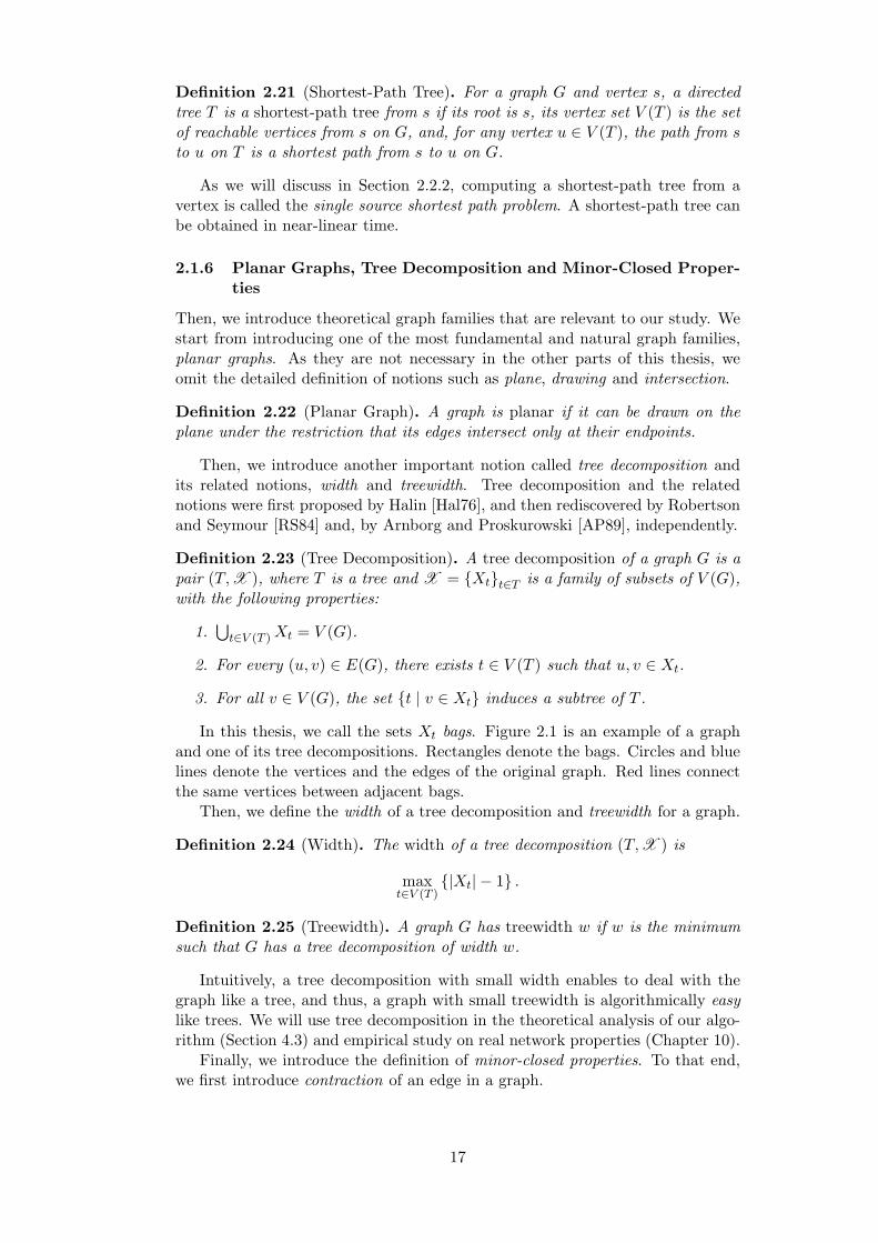
In this thesis, we call the sets Xt bags. Figure 2.1 is an example of a graphand one of its tree decompositions. Rectangles denote the bags. Circles and bluelines denote the vertices and the edges of the original graph. Red lines connectthe same vertices between adjacent bags.

Then, we define the width of a tree decomposition and treewidth for a graph.

Definition 2.24 (Width). The width of a tree decomposition (T,X ) is

maxt∈V (T )

|Xt| − 1 .

Definition 2.25 (Treewidth). A graph G has treewidth w if w is the minimumsuch that G has a tree decomposition of width w.

Intuitively, a tree decomposition with small width enables to deal with thegraph like a tree, and thus, a graph with small treewidth is algorithmically easylike trees. We will use tree decomposition in the theoretical analysis of our algo-rithm (Section 4.3) and empirical study on real network properties (Chapter 10).

Finally, we introduce the definition of minor-closed properties. To that end,we first introduce contraction of an edge in a graph.

17

0

12

3

4

5

6

7

8

9

(a) A graph

8

9

2

3

4

0

1

3

4

1

3

4

5

4

5

6

7

4

5

7

8

(b) One of its tree decom-positions

Figure 2.1: An example of tree decomposition.

Definition 2.26 (Contraction). Given a graph G = (V,E) and an edge e =(u, v) ∈ E, contracting edge e converts the graph G to G′ = (V ′, E′), where,letting ve be a new vertex, V ′ = (V \u, v)∪ve and E′ is obtained by removinge and replacing the occurrence of u and v by ve.

Roughly speaking, contraction of an edge e = (u, v) is an operation of remov-ing the edge e and merging u and v into a new vertex. Intuitively, contraction ofan edge is to make the edge shorter and shorter until its endpoints meet.

Then, we define minor and minor-closed property.

Definition 2.27 (Minor). A graph H is called a minor of a graph G if H isobtained from G by removing vertices, removing edges, and contracting edges.

Definition 2.28 (Minor-closed Property). A graph property P is minor-closedif any minor of a graph satisfying P satisfies P .

As easily observed, minor-closed properties are generalization of planarity andbounded treewidth, That is, planarity is a minor-closed property, and havingbounded treewidth is another minor-closed property.

Seemingly, minor closeness is a quite simple and natural class of graph prop-erties, but actually it has turned out that the minor closeness of a graph familysolely gives strong information on it. One of the most notable results on minorcloseness is Robertson-Seymour theorem (also known as the graph minor theo-rem) [RS04], which states that any minor-closed property is determined by a finiteset of forbidden minors. This is generalization of Kuratowski’s theorem [Kur30](or Wagner’s theorem [Wag37]) for planar graphs.

We will also use some part of the fertile results on minor-closed properties inthe theoretical analysis of our algorithm (Section 6.3).

2.1.7 Dynamic Graphs

In this thesis, we sometimes consider dynamic graphs. We basically model adynamic graph as a time series of graphs, and use symbol Gτ to denote the

18

network at time τ . For simplicity, we assume time is described by positive integers(i.e., graph snapshots are G1, G2, . . .), and we define G0 as an empty graph, i.e.,G0 = (∅, ∅). We use symbol G to denote the latest network.

We denote the distance between vertices u, v in graph Gτ by dτ (u, v). For edge(u, v) ∈ G, we define t(u, v) = τ , where τ is the time when the edge appeared inthe graph (i.e., (u, v) 6∈ E(Gτ−1) and (u, v) ∈ E(Gτ )).

2.2 Fundamental Graph Algorithms

2.2.1 Algorithm Evaluation Criteria

In this thesis, emphasis is largely put on practical performance. Therefore, ourmain evaluation criteria is the real performance numbers on modern computersystems against real network datasets.

We sometimes use synthetic networks, but we prefer real graphs. This isbecause state-of-the-art methods are designed to exploit the common structureson real graphs, and, unfortunately, current synthetic models of networks are notsufficiently similar to real networks. Experimental results on synthetic graphsare often different from those on real graphs.

On the other hand, we also sometimes discuss theoretical complexities. Formeasuring time and space complexities, we assume the word RAM model. In theword RAM model with word length b, each register can hold an integer rangingfrom 0 to 2b − 1. Operations among registers such as addition, subtraction,bit shifts and bit-wise operations can be done in constant time. Registers aremanaged like an array, and indirect addressing is capable.

2.2.2 Single Source Shortest Path Algorithms

The single source shortest path (SSSP) problem is, given a graph G = (V,E) anda source vertex s ∈ V , to compute a shortest-path tree from s or distance from sto all other vertices.

For an unweighted graph, a breadth-first search (BFS) can compute them inO(n + m) time. For a DAG, even if it is weighted, they can be obtained byconducting dynamic programming in O(n+m) time.

For a weighted graph, Dijkstra’s algorithm [Dij59] can be applied if weight ofany edge is non-negative. It runs in O(n2) time when not using priority queues.If we use standard priority queues such as binary heaps, it works in O(m log n)time. In theory, sophisticated priority queues such as fibonacci heaps [FT87]improve the time complexity to O(m+ n log n), but it is slow in practice due tohidden large constant factor. For an undirected graph with non-negative weight,Thorup’s algorithm [Tho99] have the best time complexity of O(n+m) time, butit is also slow in practice.

For a weighted graph that may contain negative weight, these algorithmsdo not work correctly, and thus Bellman-Ford algorithm [Bel58, For56] is oftenemployed. Its worst-case time complexity is O(nm) time, but implementationsusing queues work much faster in practice than what is expected from the timecomplexity.

2.2.3 All Pairs Shortest Path Algorithms

The all pairs shortest path (APSP) problem is, given a graph G = (V,E), tocompute shortest-path trees from all the vertices or distances from any pair of

19

vertices. The obvious solution to this problem is to conduct a SSSP algorithmfor n times from each vertex.

On the other hand, there are some algorithms designed for the APSP problem.The Warshall-Floyd algorithm is a popular algorithm [War62, Flo62], which isbased on very simple dynamic programming and runs in O(n3) time. Whileits asymptotic time complexity is the same as conducting Dijkstra’s algorithmwithout priority queues, The Warshall-Floyd algorithm is much faster becauseof its simpleness. However, as the real graphs that we deal with in this thesishave much less edges than Θ(n2), and thus the former approach based on SSSPis much more efficient.

In theory, APSP algorithms based on algebraic approach have been also pro-posed. In particular, for undirected graphs with small weights, the algorithmbased on matrix multiplication runs in O(M(n) · polylog(n)), where M(n) is thetime complexity of the multiplication of two n×n matrices [Car71]. The currentfastest matrix multiplication algorithm is by Le Gall [LG14] with M(n) = O(nω)where ω < 2.3728639. However, these algorithms are too complex to implement,and also their empirical performance is not believed to be promising because ofhuge hidden constant factors.

2.3 Common Structural Properties of Real-world Graphs

Finally, in this section, we review the common structural properties of real-worldgraphs of our interest. The graph data that we deal with in this thesis canbe roughly classified into two families: complex networks and road networks,where complex networks comprise various but structurally similar networks suchas social networks, web graphs and computer networks. We review the structuralproperties of these two families.

2.3.1 Complex Networks

The structural properties of complex networks have been intensively studied inthe Web, data mining and network science communities. Among many findings sofar, we introduce those that are representative or closely related to our subsequentdiscussion.

Power-law Degree Distribution The degree distribution of various complexnetworks roughly follow a power-law [BA99,FFF99,MMG+07]. That is, for someconstant γ, the fraction p(k) of the vertices with degree k is proportional tok−γ , i.e., p(k) ∝ k−γ . A power-law means that there are likely a few verticesthat have exceptionally high degree, and many vertices have degree below theaverage, leading to the existence of highly central vertices (or hubs). Parameterγ is called power exponent, where 2 < γ < 3 in most networks.

Small Average Distance and Small Diameter Average distance and diam-eters of complex networks are much smaller than what is intuitively expected fromthe numbers of vertices. This is probably famous for social networks together withthe phrase “six degrees of separation” [Mil67,TM69]. Recently, on Facebook so-cial network data, average distance is measured as 4.74, which rewrites the phraseto “four degrees of separation” [BBR+12,BV12].

20

Large Clustering Coefficient Intuitive explanation of the clustering coeffi-cient is the probability that “a friend of a friend” is a friend [HL71]. Global clus-tering coefficient considers any pair of “a friend of a friend”, while local clusteringcoefficient considers only friends of a person. It is known that, for real complexnetworks, global clustering coefficient is much larger than what is expected fromrandom edge connection [HL71,WS98,MMG+07]. Moreover, local clustering co-efficient is quite high especially for vertices with small degree [MMG+07]. Thisindicates that real complex networks have some kind of locality.

Core-Fringe Structure Generally, the core-fringe structure, core-peripherystructure or core-whisker structure of complex networks state that a network canbe roughly classified into two parts: the core part and fringe part, where thecore part is relatively dense and well connected, while the fringe part is tree-like [RPFM14,MMG+07,CSTW12,MAIK14]. With regard to formal definitionof the core-fringe structure, several different formulations have been proposed.Among them, Maehara et al. proposed that a core is a expander-like subgraphand a fringe is a subgraph of small treewidth [MAIK14], which is quite useful foralgorithm designers because these two notions are closely related to graph theoryand graph algorithms.

2.3.2 Road Networks

In contrast to complex networks, the structural property and its modeling is notas popular for road networks. This is probably because the structure of roadnetworks is much more intuitive and seemingly straightforward. However, for us,algorithm designers, since we need to design algorithms for road networks, thestructural properties of road networks are also important.

Small Separators While road networks are not precisely planar, they are closeto planar graphs. Therefore, they share several common properties to planargraphs. Among them, existence of small separators is quite useful when designingalgorithms [Tho04, KMS06, ADGW11]. It indicates that road networks can bedecomposed into parts by removing relatively small set of edges or vertices.

Highways In contrast to general planar graphs, there are highways in roadnetworks. Highways usually have higher average speed than other roads, andthus, one likely pass through highways when traveling long distance. In otherwords, long shortest paths are likely pass through (parts of) paths that correspondhighways. Therefore, compared with complex networks, while complex networkshave highly central vertices (i.e., hubs), road networks may not have verticesthat are as central as these vertices, but instead, they have very popular paths(i.e., highways). This is our motivation of our highway-based labeling frameworkintroduced in Chapter 7, which enable explicitly exploiting these highway paths.

21

Chapter 3

Review of Graph Indexing Methods

In this chapter, we review previous graph indexing methods for path-relatedqueries. As mentioned above, in this field, theoretical and practical methods arealmost totally independent. Since we focus on practical indexing methods in thisthesis, in this chapter, we also mainly review previous practical methods. Fortheoretical results, we refer to [Som14]. In particular, as our method is closelyrelated to indexing methods for distance queries on complex networks, thesemethods are of main interest in this chapter.

3.1 Shortest-path and Distance Queries on Complex Networks

For simplicity, we explain methods for answering distance queries, but it is alsoeasy for almost all the methods to simultaneously answer the shortest paths.Methods are classified into two groups: exact methods and approximate meth-ods. Exact methods always answer correct distance, while answers of approxi-mate methods may contain error. In this section, we assume that given graph isundirected and unweighted, but discussion can be naturally extended for directedand/or weighted graphs.

3.1.1 Labeling Methods

Large portion of these methods can be considered as labeling methods. Therefore,we first introduce labeling methods. Labeling methods are defined as indexingmethods that precompute a label L(v) for each vertex v, and answer a distancequery between vertices s and t only by using two labels L(s) and L(t).

In this thesis, we refer to the data structure and query algorithm of a labelingmethod as a labeling framework. Most of the previous methods are based on thelabeling framework called 2-hop cover [CHKZ03]. Our method also follows thisframework.

Index Data Structure

For each vertex v, we precompute a label denoted as L(v), which is a set of pairs(u, δuv), where u is a vertex and δuv = dG(u, v) (Figure 3.1a). We sometimes callthe set of labels L(v)v∈V as an index. We call the index correct if it satisfiesthe following conditions.

Definition 3.1 (2-Hop Cover Index for Distance Queries [CHKZ03]). Set oflabels L(v)v∈V is a (correct) 2-hop cover index for distance queries of graphG = (V,E) if L(v) is a set of pairs (u, δuv), where u is a vertex and δuv = dG(u, v),and, for any pair of vertices s, t ∈ V ,

22

𝑙1

𝑙2

𝑙3

𝒗

𝛿1

𝛿2

𝛿3

(a) An illustration of a 2-hoplabel

𝑡𝑠

(b) The query algorithm of the 2-hop cover framework

Figure 3.1: The index data structure and query algorithm of the 2-hop coverframework.

1. L(s) ∩ L(t) = ∅ if dG(s, t) =∞, and

2. min δvs + δvt | (v, δvs) ∈ L(s), (v, δvt) ∈ L(t) = dG(s, t) if dG(s, t) 6=∞.

For directed graphs, two labels are computed and stored for each vertex,called a forward label and backward label. Hierarchical 2-hop covers [ADGW12](also called hierarchical hub labelings) are a natural special class of 2-hop coversdefined below.

Definition 3.2 (Hierarchical 2-Hop Cover [ADGW12]). A 2-hop cover indexL(v)v∈V is a hierarchical 2-hop cover index of graph G = (V,E) if the relation-ship “vertex v is in the label of vertex w” defines a partial order on the vertex setV .

Moreover, canonical 2-hop covers [ADGW12] (also called canonical hub label-ings) are a further special class of hierarchical 2-hop covers. Recent algorithms,including our pruned labeling algorithm, compute canonical 2-hop covers. Canon-ical 2-hop covers are defined as follows.

Definition 3.3 (Canonical 2-Hop Cover [ADGW12]). For a graph G = (V,E), a2-hop cover index L(v)v∈V is a canonical 2-hop cover index of G if, for a totalorder r of vertices, L(s) is the set of vertices that ranks the highest in PG(s, t)with respect to r for any vertex t.

Note that, given a total order, the canonical 2-hop cover is unique.

Query Algorithm

To answer a distance query between vertices s and t, we compute and answerQuery(s, t, L) defined as follows (Figure 3.1b),

Query(s, t, L) = min δvs + δvt | (v, δvs) ∈ L(s), (v, δvt) ∈ L(t) .

We define Query(s, t, L) = ∞ if L(s) and L(t) do not share any vertex. It isobvious that, if L is a correct 2-hop cover index, Query(s, t, L) = dG(s, t) forany pair of vertices s and t.

For each vertex v, we store the label L(v) so that pairs in it are sorted bytheir vertices. Then, we can compute Query(s, t, L) in O(|L(s)| + |L(t)|) timeusing a merge-join-like algorithm.

23

Indexing Algorithms

As we have seen above, the indexing framework (i.e., the index data structureand query algorithm) of the 2-hop cover framework is simple. However, findingsmall 2-hop covers efficiently is a challenging and long-standing problem. Asthe minimization of the size of labels is proven to be NP-hard, approximatealgorithms and heuristic algorithms have been studied.

In the original work [CHKZ03], Cohen et al. proposed an approximate labelingalgorithm that guarantees the approximation ratio of O(log n) from the optimal2-hop cover. However, the algorithm first computes the distance matrix, thenreduces the label computation to an optimization problem. Therefore, the scal-ability is highly limited. A faster labeling algorithm built on this approach withthe same approximation guarantee was recently presented by Delling et al., whichis orders of magnitude better than previous algorithm [DGSF14]. Nevertheless,it can process networks with at most tens of thousands of edges.

More scalable algorithm that computes canonical 2-hop covers was pro-posed by Delling et al. [ADGW12]. It is based on a method for road net-works [ADGW11], which will be introduced in later sections. It first constructshierarchical 2-hop covers through contraction hierarchies, then it reduces the la-bel sizes by making them canonical. It also requires Θ(n2) space.

Extensions

A variant related to 2-hop cover is highway-centric labeling [JRXL12]. In thismethod, we first compute a spanning tree T and use it as a “highway”. That is,when computing distance dG(u, v) between two vertices u and v, we output theminimum over dG(u,w1)+dT (w1, w2)+dG(w2, v) where w1 and w2 are vertices inlabels of u and v, respectively, and dT (·, ·) is the distance metric on the spanningtree T .

IS-Label is another method that combines partial 2-hop cover and online graphsearches [FWCW13]. To create an index, it recursively computes a vertex coverand reduce vertices in the corresponding independent set. Simultaneously, it addslabel entries to the labels of these removed vertices. The recursion is stoppedwhen the graph gets sufficiently small. To answer queries, it reduces the problemto many-to-many distance computation on the reduced graph by using the partial2-hop labels.

3.1.2 Tree-Decomposition-Based Methods

An approach based on heuristic tree decomposition is also reported to be ef-ficient [Wei10, ASK12]. Tree decomposition and complex networks are seem-ingly unrelated at first glance, as intuitively treewidth of complex networksis not small. However, because of the core–fringe structure of these net-works [CNSW00,NSW01], the fringe part is actually tree-like, and these methodsexploit the tree-like structure by tree decomposition.

Index Data Structure

Since complex networks do not have small treewidth, to exploit the tree-likefringes, new notion of relaxed tree decomposition is used in these methods.

Definition 3.4 (Relaxed Tree Decomposition [Wei10,ASK12]). A tree decompo-sition is called a relaxed tree decomposition with width w if all bags except forone have size at most w + 1.

24

We call the one arbitrary large bag the root bag. As an index, these methodsprecompute and store a tree decomposition and a distance matrix for each bagof it. The index size is O(nw2 + r2), where w is the relaxed width of the treedecomposition, and r is the size of the root bag.

Indexing Algorithm

They compute a tree decomposition by algorithms built on the min-degree heuris-tic algorithm [BHS03]. As we will also use the min-degree heuristic in Chapter 10,we will explain the algorithm later.

The original method proposed by Wei [Wei10] computes the distance matri-ces after obtaining tree decompositions (Figure 3.2). In contrast, Akiba et al.proposed to simultaneously compute the distance matrices on reduced graphs ofmin-degree heuristics [ASK12]. This technique improved the scalability by anorder of magnitude.

6 8 10

6 0 2 1

8 2 0 2

10 1 2 0

5 6 8

5 0 1 1

6 1 0 2

8 1 2 0

Figure 3.2: The index construction process of tree-decomposition-based ap-proaches.

Query Algorithm

To answer queries, we conduct dynamic programming on the trees (Figure 3.3).The basic algorithm by Wei works as follows [Wei10]. We start from two bagsthat contain the specified endpoints. We ascend the bags by computing distancesfrom endpoints to vertices in each bag. We stop the process at the lowest commonancestor of the two bags. It works in O(w2h) time, where h is the height of thetree decomposition. Akiba, et al. proposed more sophisticated query algorithmsthat work in O(w2 log h) time [ASK12].

3.1.3 Landmark-based Methods

To gain more scalability than these exact methods, approximate methods, whichdo not always answer correct distances, also have been studied. The major ap-proach is the landmark-based approach [TC03,VFD+07].

The basic idea of these methods is to select a subset L of vertices as landmarks,and precompute the distance dG(`, u) between each landmark ` ∈ L and all thevertices u ∈ V . When the distance between two vertices u and v is queried, weanswer the minimum dG(u, `) + dG(`, v) over landmarks ` ∈ L as an estimate.

Generally, the precision for each query depends on whether actual shortestpaths pass nearby the landmarks. Therefore, by selecting central vertices as land-marks, the accuracy of estimates becomes much better than selecting landmarks

25

1 2 3 4

1 2 3 4

2 3

V 1 2

Dist 0 1

V 2 3

Dist 1 2

V 3 4

Dist 1 0

V 2 3

Dist 2 1

+1

+1 +1

+1

Distance from 1 Distance to 4

Original Graph

Tree Decomposition

Figure 3.3: The query algorithm of tree-decomposition-based distance querying.

randomly [PBCG09, CSTW12]. However, for close pairs, the precision is stillmuch worse than the average, since lengths of shortest paths between them aresmall and they are unlikely to pass nearby the landmarks [ASK12].

To further improve the accuracy, several techniques were proposed [GBSW10,TACGBn+11,QCCY12]. They typically store shortest-path trees rooted at thelandmarks instead of just storing distances from the landmarks. To answerqueries, they extract paths from the shortest-path trees as candidates of shortest-paths, and improve them by finding loops or shortcuts. While they significantlyimprove the accuracy, the query time becomes up to three orders of magnitudeslower.

3.2 Shortest-path and Distance Queries on Road Networks

Shortest-path distance queries on road network has a larger body of research. Inthis section, we focus on two representative recent methods that are related withmethods of our interest: contraction hierarchies and labeling methods. Exhaus-tive survey is given in [BDG+14], and detailed experimental comparison of recentmethods is given in [WXD+12]. In this section, as we deal with road networks,we assume that given graph G = (V,E) is weighted and has a weight function w.

3.2.1 Contraction Hierarchies

The idea based on contraction hierarchies is just to repeatedly contract vertices byincreasing order of importance to obtain two DAGs (upward graph and downwardgraph), on which query algorithms can efficiently obtain shortest-paths [GSSD08].

Index Data Structure

From the given graph, indexing algorithms construct two weighted DAGs, upwardgraph G↑ = (V,E↑) and downward graph G↓ = (V,E↓). The two DAGs respecta total order of vertices called importance in a reverse way. That is, for any(u, v) ∈ E↑, u has a lower importance than v, and, for any (u, v) ∈ E↓, u hasa higher importance than v. A weighted graph G′ = (V,E↑ ∪ E↓) is called acontraction hierarchy of the graph G.

26

Indexing Algorithm

We construct a contraction hierarchy basically by repeatedly contracting vertices(Figure 3.4). First, both of the upward and downward graph are initialized withthe edges of original graph with the corresponding directions. Contraction of avertex v is to remove vertex v and add edges that are necessary not to changethe distance between at least one pair of remaining vertices.

When contracting less important vertices, as shortest paths are less likely topass these vertices, new edges are less likely to be added. Therefore, vertices arecontracted by increasing order of importance. The order is heuristically deter-mined simultaneously with contraction process.

Query Algorithm

The query algorithm is just to compute a shortest path from two endpoints inthe contraction hierarchy G′. We can conduct bidirectional search on it.

Relation to Tree-Decomposition-Based Methods

Interestingly, indexing algorithms of contraction hierarchies have much in com-mon with tree-decomposition-based methods introduced above. As we will ex-plain in Chapter 10 the min-degree heuristic algorithm computes tree decomposi-tions by reducing vertices. This reduction process is quite similar to the contrac-tion above. However, one crucial difference is that, while the tree decompositionprocess adds edges between every pair of neighbors, the contraction process onlyadds necessary edges for remaining shortest paths. If we add only necessary edgesduring tree decomposition, obtained decompositions would not be a tree decom-position. On the other hand, as the contraction hierarchy algorithm adds lessedges, it seems to be more scalable.

However, there is also difference of index data structures; while the contrac-tion hierarchies are union of DAGs, tree decompositions can be processed liketrees and thus query algorithms can be more efficient. While these methods aredeveloped independently in different communities (the database community andexperimental algorithmics community), and also targeted graphs are different,they turned out to be interestingly related.

Contraction hierarchies have also interesting relation to labeling-based meth-ods, which will be introduced in the next section.

3.2.2 Labeling Methods

The recent emergence of practical labeling methods for distance queries on roadnetworks is quite interesting and indeed a rare example of practical impact oftheoretical research in this field. In the seminal theoretical work by Abrahamet al. [AFGW10], they theoretically analyzed the indexing algorithms for dis-tance queries on road networks under their new notion of highway dimension.Interestingly, their theoretical result suggested that there should be good labelson road networks, whereas previously little effort has been done for labeling-basedmethods. Then, in their follow-up empirical work, Abraham et al. demonstratedthat indeed the labeling approach is practical on continental-scale road networksof the day [ADGW11].

The labeling framework (i.e., the index data structure and query algo-rithm) used for distance queries on road networks is exactly the 2-hop cover

27

６ １ ４ ３ ５２２２ ２２ １３

(a)

６

１

４ ３ ５２２ ２

２

１

３

５

(b)

６

１

４ ３ ５

２

２

２

２

１

３

５

(c)

６

１

４

３

５

２

２

２

２

１

３

３５

(d)

６

１

４

３

５

２

２

２

２

１

３

３５

８

(e)

６

１

４

３

５

２

２２

２

１

３

３

５

８

(f)

６

１

４

３

５

２

２２

２

１

３

３

５

８

(g)

Figure 3.4: The index construction process of contraction hierarchies. Blue, yel-low and red vertices denote those which are not yet contracted, already contractedand just being contracted, respectively.

28

framework introduced above. However, please note that it is called as hub-based labeling or hub labeling in the field of distance queries on road net-works [ADGW11,ADGW12].

Hierarchical Labels through Contraction Hierarchies

The first practical indexing algorithm by Abraham et al. computes labels byusing contraction hierarchies [ADGW11]. Their labels are hierarchical labels(see Definition 3.2), which respects the order of importance of the correspondingcontraction hierarchies. The basic idea is to construct the forward label of v as thevertices that can be reached from v in the upward graph G↑, and to construct thebackward label of v as the vertices that can reach v in the downward graph G↓. Itis easy to see that the labels are correct because the query algorithm correspondsthe bidirectional search on the contraction hierarchy graph. Surprisingly, theiralgorithm proved that road networks with tens of millions of vertices and edgeshad 2-hop covers with average label sizes of about one hundred. As a result,the labeling-based approach became the indexing method for distance queries onroad networks with the fastest query time.

Canonical Labeling by Pruning

Then, in their next paper, they proposed the notion of canonical labeling (Defi-nition 3.3). They also proposed a pruning algorithm to reduce the label sizes ofhierarchical labels by converting them to canonical labels. For a road network ofWestern Europe, their new indexing algorithm using the technique above reducedthe label size from 85 to 69.

Recall that canonical labeling is unique under the same vertex ordering.Therefore, both their algorithm and our algorithm compute the exactly samecanonical labeling when they are given the same vertex ordering, and both arebased on pruning. However, the algorithms are totally different and our algorithmhas much better scalability. Their algorithm first computes hierarchical labelingand then obtains canonical labeling (the latter step is called pruning), while oursdirectly computes canonical labeling during pruned graph searches. Indeed, intheir recent work [DGPW14], they also started using our labeling algorithm (seeChapter 11).

Label Compression

Because the largest disadvantage of labeling-based methods is space consump-tion, they proposed label compression schemes to reduce the space consump-tion [ADGW11,DGW13,DGPW14]. The basic idea of their compression schemeis to represent a label as a tree and reuse the common parts of different labels.Therefore, the total set of labels is represented as a DAG.

In particular, the underlying thought in [DGW13] is, again, interestingly con-nected with contraction hierarchies. Their finding is that, while they constructhierarchical 2-hop cover labels from contraction hierarchies, contraction hierar-chies can also be easily obtained from any hierarchical 2-hop cover labels byconsidering label trees. This is quite interesting because the labeling-based ap-proach is one of the heaviest indexing approaches, while the contraction hierar-chy approach is one of the most lightweight indexing approaches, in the sense ofthe trade-off between index size and query time. Therefore, their compressionscheme is designed to combine the contraction-hierarchy-like index structure intothe labeling-based approach.

29

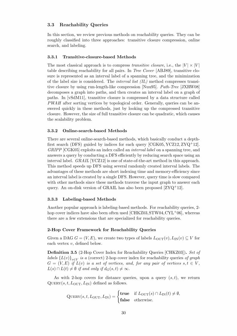
3.3 Reachability Queries

In this section, we review previous methods on reachability queries. They can beroughly classified into three approaches: transitive closure compression, onlinesearch, and labeling.

3.3.1 Transitive-closure-based Methods

The most classical approach is to compress transitive closure, i.e., the |V | × |V |table describing reachability for all pairs. In Tree Cover [ABJ89], transitive clo-sure is represented as an interval label of a spanning tree, and the minimizationof the label size is considered. The interval list (IL) method compresses transi-tive closure by using run-length-like compression [Nuu95]. Path-Tree [JXRW08]decomposes a graph into paths, and then creates an interval label on a graph ofpaths. In [vSdM11], transitive closure is compressed by a data structure calledPWAH after sorting vertices by topological order. Generally, queries can be an-swered quickly in these methods, just by looking up the compressed transitiveclosure. However, the size of full transitive closure can be quadratic, which causesthe scalability problem.

3.3.2 Online-search-based Methods

There are several online-search-based methods, which basically conduct a depth-first search (DFS) guided by indices for each query [CGK05,YCZ12, ZYQ+12].GRIPP [CGK05] exploits an index called an interval label on a spanning tree, andanswers a query by conducting a DFS efficiently by reducing search space using aninterval label. GRAIL [YCZ12] is one of state-of-the-art method in this approach.This method speeds up DFS using several randomly created interval labels. Theadvantages of these methods are short indexing time and memory-efficiency sincean interval label is created by a single DFS. However, query time is slow comparedwith other methods since these methods traverse the input graph to answer eachquery. An on-disk version of GRAIL has also been proposed [ZYQ+12].

3.3.3 Labeling-based Methods

Another popular approach is labeling-based methods. For reachability queries, 2-hop cover indices have also been often used [CHKZ03,STW04,CYL+06], whereasthere are a few extensions that are specialized for reachability queries.

2-Hop Cover Framework for Reachability Queries

Given a DAG G = (V,E), we create two types of labels LOUT(v), LIN(v) ⊆ V foreach vertex v, defined below.

Definition 3.5 (2-Hop Cover Index for Reachability Queries [CHKZ03]). Set oflabels L(v)v∈V is a (correct) 2-hop cover index for reachability queries of graphG = (V,E) if L(v) is a set of vertices, and, for any pair of vertices s, t ∈ V ,L(s) ∩ L(t) 6= ∅ if and only if dG(s, t) 6=∞.

As with 2-hop covers for distance queries, upon a query (s, t), we returnQuery(s, t, LOUT, LIN) defined as follows.

Query(s, t, LOUT, LIN) =

true if LOUT(s) ∩ LIN(t) 6= ∅,false otherwise.

30

We construct labels LOUT and LIN so that, for every s, t ∈ V ,Query(s, t, LOUT, LIN) matches the reachability on G from s to t. Naive cal-culation of Query(s, t, LOUT, LIN) needs O(ls · lt) time for ls = |LOUT(s)| andlt = |LIN(t)|. However, if LOUT(s) and LIN(t) are sorted, it can be done inO(ls + lt) time by scanning both labels from their heads to tails simultaneously.

While the framework is highly common to methods for distance queries intro-duced above, labeling algorithms are again designed independently and almostindependent [STW04,CYL+06]. For example, the approach proposed by Schenkelet al. is based on divide-and-conquer algorithm. The algorithm is tailored tographs that are quite close to trees such as XMLs.

Extensions of 2-Hop Covers

3-hop cover [JXRF09] is a generalization of 2-hop cover, where labels are createdto satisfy that a vertex can reach its descendants via two vertices by using chaindecomposition. These hop cover methods usually achieve small query time andindex size, but computing such good labels is prohibitively expensive on large-scale graphs.

3.3.4 General Improving Techniques

There are some general techniques to improve the performance of reachabilityindices. The idea of query preserving compression [FLWW12] is to make a com-pressed graph with which we can correctly answer reachability queries on the orig-inal graph. In [JRDX12], a reachability computation framework named SCARABwas proposed. In the framework, a smaller graph called a reachability backboneis constructed from an input graph and a reachability query on the original graphcan be answered by issuing several reachability queries on the reachability back-bone. These techniques can be combined with any methods, including ours, andmake them more scalable.

3.4 Theoretical Results

As mentioned in Chapter 1, most of the results from the theoretical algorithmcommunity are of independent interest from practical efficiency. By contrast,there are a few notable theoretical results that offer valuable insight also intoempirical algorithmics on graph indexing. In this section, we introduce theseresults.

3.4.1 Highway Dimension

Real road networks are close to planar graphs, but they are not exactly planar.For example, there are grade separated crossings. Moreover, even if we assumeroad networks are planar, still, it is not sufficient to theoretically explain theefficiency of practical indexing methods for distance queries on road networks.Intuitively, these practical indexing models exploit more specific structures ofroad networks, e.g., existence of popular roads such as highways.

To theoretically discuss the efficiency of algorithms on such road net-works, Abraham et al. proposed a new theoretical notion called highway dimen-sion [AFGW10]. They modeled road networks as graphs with small highwaydimension. Intuitively, a graph with small highway dimension is one that hassmall sets of vertices where any long shortest paths pass through at least one of

31

them. This assumption coincides our intuitive understanding of the structure ofreal road networks.

Under the assumption of small highway dimension, those practical indexingmethods are theoretically proved to be efficient for the first time. Moreover, aswe mentioned above, the results also motivated the use of the labeling approachfor distance queries on road networks, which has been indeed demonstrated tobe prominent.

3.4.2 Power-Law Random Graphs

As with the discussion above, to discuss distance querying on complex networkssuch as social and web graphs, there also should be assumptions for graphs. Aswe explained above, practical methods exploit the common structures of thesenetworks, and thus analysis on general graphs are unfortunately not very inter-esting.

To address this issue, Chen et al. presented the first theoretically interest-ing results about distance queries on graphs with power-law degree distribu-tion [CSTW12]. They assumed fixed degree random graph, and they conductedrigorous average case analysis on the theoretical indexing method by Thorupand Zwick [TZ05]. The results theoretically confirmed our intuition that highlycentral vertices (i.e., hubs) in these networks make shortest path computationeasier.

32

Chapter 4

Basic Form of Pruned Landmark Labeling

Algorithm

In this chapter, we present the basic form of the pruned landmark labeling al-gorithm. Here, we assume that the given graph G = (V,E) is undirected andunweighted. We only consider basic distance queries, i.e., we construct an indexto efficiently answer distances between arbitrary pairs of vertices. As the indexdata structure, we use the original 2-hop cover framework explained in Chapter 3.

We first explain the offline labeling algorithm and prove its correctness (Sec-tion 4.1). Then, we discuss vertex ordering for empirically exploiting the struc-tures of real networks (Section 4.2). Next, we look into theoretical properties ofour labeling algorithm to further see that, with proper vertex ordering strategies,it can exploit various structures of real networks (Section 4.3). In Section 4.4,common engineering techniques for efficient implementation are presented. Fi-nally, we discuss online update algorithms of 2-hop indices for dynamic graphupdate based on pruned labeling (Section 4.5).

In this chapter, we do not present experimental results. Experimental evalu-ation will be presented in the following chapters, which deal with more concreteproblem settings on real instances. This chapter presents the concept of prunedlabeling that is common to the methods tailored to each problem setting.

4.1 Labeling Algorithm

We explain our labeling algorithm (i.e., an indexing algorithm for the 2-hop coverframework) in two steps. We start with the following naive method, and then weintroduce pruning to the method.

4.1.1 Naive Landmark Labeling

Our naive landmark labeling algorithm conducts a BFS from each vertex andstore distances between all pairs as an index. Though this method is too obviousand inefficient, for the exposition of the next method, we explain the details.

Let V = v1, v2, . . . , vn. We start with an empty index L0, where L0(u) =∅ for every u ∈ V . Suppose we conduct BFSs from vertices in the order ofv1, v2, . . . , vn. After the k-th BFS from a vertex vk, we add distances from vk tolabels of reached vertices, that is, Lk(u) = Lk−1(u) ∪ (vk, dG(vk, u)) for eachu ∈ V with dG(vk, u) 6=∞. We do not change labels for unreached vertices, thatis, Lk(u) = Lk−1(u) for every u ∈ V with dG(vk, u) =∞.

Ln is the final index. Obviously Query(s, t, Ln) = dG(s, t) for any pair ofvertices s and t, and therefore, Ln is a correct 2-hop cover for exact distance

33

Algorithm 4.1 Pruned BFS from vk ∈ V to create index L′k.

1: procedure PrunedBFS(G, vk, L′k−1)

2: Q← a queue with only one element vk.3: P [vk]← 0 and P [v]←∞ for all v ∈ V (G) \ vk.4: L′

k[v]← L′k−1[v] for all v ∈ V (G).

5: while Q is not empty do6: Dequeue u from Q.7: if Query(vk, u, L

′k−1) ≤ P [u] then

8: continue9: L′

k[u]← L′k−1[u] ∪ (vk, P [vk])

10: for all w ∈ NG(v) s.t. P [w] =∞ do11: P [w]← P [u] + 1.12: Enqueue w onto Q.

13: return L′k

queries. This is because, if s and t are reachable, then (s, 0) ∈ Ln(s) and(s, dG(s, t)) ∈ Ln(t) for example.

This method can be considered as a variant of landmark-based approxi-mate methods, which we mentioned in Section 3. The standard landmark-basedmethod can be regarded as a method that precomputes Ll instead of Ln and es-timates distance between s and t by Query(s, t, Ll), where l n is a parameterexpressing the number of landmarks.

4.1.2 Pruned Landmark Labeling

Then, we introduce pruning to the naive method. Similarly to the method above,we conduct pruned BFSs from vertices in the order of v1, v2, . . . , vn. We startwith an empty index L′

0 and create an index L′k from L′

k−1 using the informationobtained by the k-th pruned BFS from vertex vk.

We prune BFSs as follows. Suppose that we have an index L′k−1 and we are

conducting a BFS from vk to create a new index L′k. Suppose that we are visiting

a vertex u with distance δ. If Query(vk, u, L′k−1) ≤ δ, then we prune u, that is,

we do not add (vk, δ) to L′k(u) (i.e. L

′k(u) = L′

k−1(u)) and we do not traverse anyedge from vertex u. Otherwise, we set L′

k(u) = L′k−1(u) ∪ (vk, δ) and traverse

all the edges from the vertex u as usual. As with the previous method, we also setL′k(u) = L′

k−1(u) for all vertices u ∈ V that were not visited in the k-th prunedBFS. This algorithm, performing pruned BFSs, is described as Algorithm 4.1,and the whole preprocessing algorithm is described as Algorithm 4.2.

Figure 4.1 shows examples of pruned BFSs. The first pruned BFS fromvertex 1 visits all the vertices (Figure 4.1a). During the next pruned BFSfrom vertex 2 (Figure 4.1b), when we visit vertex 6, since Query(2, 6, L′

1) =dG(2, 1) + dG(1, 6) = 3 = dG(2, 6), we prune vertex 6 and we do not traverseedges from it. We also prune vertices 1 and 12. As the number of performedBFSs increases, we can confirm that the search space gets smaller and smaller.

4.1.3 Proof of Correctness

In the following, we prove that this method computes a correct 2-hop cover index,that is, Query(s, t, L′

n) = dG(s, t) for any pair of vertices s and t.

Theorem 4.1. For any 0 ≤ k ≤ n and for any pair of vertices s and t,Query(s, t, L′

k) = Query(s, t, Lk).

34

1

46

7

8

9

1012

2

3

5

11

(a)

1

4

7

9

12

2

5

8

10

3

6

11

(b)

1

4

7

9

28

3

11

12

56

10

(c)

1

7

9

12

28

10

3

4

56

11

(d)

1

4

7

9

12

28

10

3

65

11

(e)

1

4

7

9

12

28

10

3

56

11

(f)

1

4

9

12

28

10

3

56

7

11

(g)

1

4

7

9

12

2

10

3

56

8

11

(h)

1

4

7

12

28

10

3

56

9

11

(i)

1

4

7

9

12

28

3

56

10

11

(j)

1

4

7

9

12

28

10

3

56

11

(k)

1

4

7

9

28

10

3

56

11

12

(l)

Figure 4.1: Examples of pruned BFSs. Yellow vertices denote the roots, bluevertices denote those which we visited and labeled, red vertices denote thosewhich we visited but pruned, and gray vertices denote those which are alreadyused as roots.

35

Algorithm 4.2 Compute a 2-hop cover index by pruned BFS.

1: procedure Preprocess(G)2: L′

0[v]← ∅ for all v ∈ V (G).3: for k = 1, 2, . . . , n do4: L′

k ← PrunedBFS(G, vk, L′k−1)

5: return L′n

Proof. We prove the theorem by mathematical induction on k. Since L′0 = L0,

it is true for k = 0. Now we assume it holds for 0, 1, . . . , k − 1 and prove it alsoholds for k.

Let s, t be a pair of vertices. We assume these vertices are reachable in G, sinceotherwise the answer∞ can be obviously obtained. Let j be the smallest numbersuch that (vj , δvjs) ∈ Lk(s), (vj , δvjt) ∈ Lk(t) and δvjs + δvjt = Query(s, t, Lk).We prove that (vj , δvjs) and (vj , δvjt) are also included in L′

k(s) and L′k(t). This

immediately leads to Query(s, t, L′k) = Query(s, t, Lk). Due to the symmetry

between s and t, we prove (vj , δvjs) ∈ L′k(s).

First, for any i < j, we prove by contradiction that vi 6∈ PG(vj , s). If weassume vi ∈ PG(vj , s), from Inequality 2.1

Query(s, t, Lk) = dG(s, vj) + dG(vj , t)

= dG(s, vi) + dG(vi, vj) + dG(vj , t)

≥ dG(s, vi) + dG(vi, t).

Since (vi, dG(s, vi)) ∈ Lk(s) and (vi, dG(t, vi)) ∈ Lk(t), this contradicts to theassumption of the minimality of j. Therefore, vi 6∈ PG(vj , s) holds for any i < j.

Now we prove that (vj , dG(vj , s)) ∈ L′k(s). Actually, we prove a more general

fact: (vj , dG(vj , u)) ∈ L′k(u) for all u ∈ PG(vj , s). Note that s ∈ PG(vj , s).

Suppose that we are conducting the j-th pruned BFS from vj to create Lj . Letu ∈ PG(vj , s). Since PG(vj , u) ⊆ PG(vj , s) and vi 6∈ PG(vj , s) for any i < j, wehave vi 6∈ PG(vj , u) for any i < j. Therefore, Query(vj , u, L

′j−1) > dG(vj , u)

holds. Thus, we visit all vertices u ∈ PG(vj , s) without pruning, and it followsthat (vj , dG(vj , u)) ∈ L′

j(u) ⊆ L′k(u).

As a corollary, our method is proved to be an exact distance querying methodby instantiating the theorem with k = n.

Corollary 4.1. For any pair of vertices s and t,

Query(s, t, L′n) = dG(s, t).

4.2 Vertex Ordering Strategies

In the algorithm description above, we conducted pruned BFSs from vertices inthe order of v1, v2, . . . , vn. We can freely choose the order, and moreover it turnsout that the order is crucial for the performance of this method as we will see inthe experimental results presented in Section 5.2.3.

To decide the order of vertices, we should select central vertices first in thesense that many shortest paths pass through these vertices. Since we would liketo prune later BFSs as much as possible, we want to cover larger part of pairs ofvertices by earlier BFSs. That is, the earlier labels should offer correct distancesfor as many pairs of vertices as possible, and therefore the earlier vertices shouldbe those who many shortest paths passes through.

36

This problem is quite similar to the problem of selecting good landmarks forlandmark-based approximate methods, which is discussed well in [PBCG09]. Inthat problem, we also want to select good landmarks so that many shortest pathpasses through these vertices or nearby vertices.

This part of our algorithm highly depends on the structures of graphs. There-fore, we leave this part until we consider concrete problem settings. In fact, onnetworks with skewed degree distribution (e.g., complex networks), simple strate-gies work surprisingly well, as we will see in Section 5.2.3. On the other hand, forroad networks, we need different strategies, as the degree gives little informationabout each vertex on these networks.

4.3 Theoretical Properties

4.3.1 Minimality

Theorem 4.2. Let L′n be the index defined in Section 4.1.2. L′

n is minimal inthe sense that, for any vertex v and for any pair (u, δuv) ∈ L′

n(v), there is a pairof vertices (s, t) such that, if we remove (u, δuv) from L′

n(v), we cannot answerthe correct distance between s and t.

Proof. Let vi ∈ V and (vj , δvjvi) ∈ L′n(vi). This implies j < i. We show that

if we remove (vj , δvjvi) from L′n(vi) then we cannot answer the correct distance

between vi and vj . We claim that, for any k 6= j, either (i) (vk, δvkvi) 6∈ L′n(vi)

or (vk, δvkvj ) 6∈ L′n(vj) holds, or (ii) dG(vi, vk) + dG(vk, vj) > dG(vi, vj) holds.

Suppose k < j and assume that (ii) does not hold. Then, (i) must hold sinceotherwise the j-th BFS should have pruned vertex vi and (vj , δvjvi) 6∈ L′

n(vi).Suppose k > j and assume that (ii) does not hold. Then, vk ∈ PG(vi, vj) andtherefore (vj , δvjvk) ∈ L′

j(vk), thus the k-th BFS prunes vertex vj , leading to(vk, δvkvj ) 6∈ L′

n(vj).

4.3.2 Canonicality of Labels

As we mentioned in Chapter 3, our labels are hierarchical (Definition 3.2).

Lemma 4.1 ( [DGPW14] ). The labels computed by the pruned landmark labelingalgorithm are canonical.

Among hierarchical 2-hop indices that respect a vertex ordering, the canon-ical labeling with respect to the vertex ordering is the only one minimal index(and thus the index is also minimum) [ADGW12]. Therefore, together with thediscussion on minimality, our labels are also canonical with respect to the vertexordering.

4.3.3 Exploiting Existence of Highly Central Vertices

Then, we compare our method with landmark-based methods to show that ourmethod also can exploit the existence of highly central vertices. We consider thestandard landmark-based method [PBCG09,VFD+07], which do not use any pathheuristics. As we stated in Chapter 3, by selecting central vertices as landmarks, itattains remarkable average precision for real-world networks. From the followingtheorem, we can observe that our method is efficient for networks whose distancecan be answered by landmark-based methods with such high precision, and ourmethod also can exploit the existence of these central vertices.

37

Theorem 4.3. If we assume that the standard landmark-based approximatemethod can answer correct distances to (1− ε)n2 pairs (out of n2 pairs) using klandmarks, then the pruned landmark labeling method gives an index with averagelabel size O(k + εn).

Proof. After conducting pruned BFSs from the k landmark vertices first, at mostεn2 pairs are added to the index in total, since we never add pairs whose distancecan be answered from current labels.

4.3.4 Exploiting Small Treewidth

Finally, we show a theoretical evidence that our method can also exploit tree-likefringes efficiently. As we explained in Chapter 3, methods based on tree decompo-sitions were proposed for distance queries [Wei10,ASK12]. Both of them extendmethods which work efficiently for graphs of small treewidth, and they exploitlow treewidth of fringes in real-world networks by tree decompositions. Inter-estingly, though we do not use tree decompositions explicitly, we can prove thatour method can efficiently process graphs of small treewidth. Thus, our methodimplicitly exploits this property of real-world networks too. For definitions oftreewidth and tree decompositions, see Chapter 2.

Theorem 4.4. Let w be the treewidth of G. There is an order of vertices withwhich the pruned landmark labeling method takes O(wm log n+ w2n log2 n) timefor preprocessing, stores an index with O(wn log n) space, and answers each queryin O(w log n) time.

Proof. We consider the centroid decomposition [Jor69] of the tree decomposition.First we conduct pruned BFSs from all the vertices in a centroid bag. Then, laterpruned BFSs never go beyond the bag. Therefore, we can consider as we dividedthe tree decomposition into disjoint components, each having at most half of thebags. We recursively repeat this procedure. The number of recurrences is at mostO(log n). Since we add at most w pairs to each vertex at each depth of recursion,the number of pairs in each label is O(w log n). At each depth of recursion, thetotal time consumed by pruned BFSs from the current components is O(wm +w2n log n), where O(wm) is the time for traversing edges and O(w2n log n) is thetime for pruning tests.

4.4 Common Techniques for Efficient Implementation

4.4.1 Preprocessing

Index: First, in the description above, we treated L′k−1 and L′

k separately andexplained as if we copy L′

k−1 to L′k for simplicity of explanation. However, this

copy can be easily avoided by keeping only one index and adding labels to it aftereach pruned BFS.

Initialization: Another important note is to avoid O(n) time initialization foreach pruned BFS. The reason why this method is efficient is that the searchspace of pruned BFSs gets much more smaller than the whole graph. Howeverif we spend O(n) time for initialization, it would be the bottleneck. What wewant to do in the initialization is to set all values in the array storing tentativedistances as∞ (Line 3). We can avoid O(n) time initialization as follows. Beforewe conduct the first pruned BFS, we set all values in the array P as ∞. (Thistakes O(n) time but we do this only once.) Then, during each pruned BFS, we

38

store all vertices we visited, and after each pruned BFS, we set P [v] as ∞ for alleach vertex v we have visited.

Arrays: For the array storing tentative distances, it is better to use 8-bit integers.Since networks of our interest are small-world networks, 8-bit integers are enoughto represent distances. Using 8-bit integers, the array fits into low-level cachememories of recent computers, resulting in the speed up by reducing cache misses.

Querying: To evaluate queries for pruning (Line 7), it is faster to use an algo-rithm different from the normal one since we can exploit the fact here that weissue many queries whose one endpoint is always vk. Before starting the k-thpruned BFS from vk, we prepare an array T of length n initialized with ∞ andset T [w] = δwvk for all (w, δwvk) ∈ L′

k−1(vk). To evaluate Query(vk, u, L′k−1), for

all (w, δwu) ∈ L′k−1(u), we compute δwu+T [w] and return the minimum. Though

normal querying algorithm takes O(∣∣L′

k−1(vk)∣∣+ ∣∣L′

k−1(u)∣∣) time, this algorithm

runs in O(∣∣L′

k−1(u)∣∣) time. As Line 7 is the bottleneck of the algorithm, this

technique speeds up preprocessing by about twice. Note that T should be rep-resented by 8-bit integers as the same reason described above, and O(n) timeinitialization for array T should be avoided in the same way for array P .

Prefetching: Unfortunately, we cannot fit the index and the adjacency lists intothe cache memory for large-scale networks. However, we can manually prefetchthem to reduce the cache misses, since vertices which we will access soon are inthe queue. Manual prefetching speeds up preprocessing by about 20%.

Thread-Level Parallelism: As with parallel BFS algorithms [APPB10], thepruned BFS algorithm can be also parallelized. However, for simple experimentalanalysis and fair comparison to previous methods, we did not parallelize ourimplementation in the experiments.

Sorting Labels: When applying merge-join-like algorithms to answer queries,pairs in labels need to be sorted by vertices. However, actually we do not needto sort explicitly by storing ranks of vertices instead of vertices. That is, whenadding a pair (u, δ) in the i-th pruned BFS from vertex u, we add a pair (i, δ)instead. Then, since pairs are added from vertices with lower rank to those withhigher rank, all the labels are automatically sorted.

4.4.2 Querying

Sentinel: We add a dummy entry, (n,∞), to the label L(v) for each v ∈ V . Thisdummy entry ensures that we find the same vertices, n, in the end when scanningtwo labels. Thus we can avoid to separately test whether we have scanned tillthe end.

Arrays: For each label L(v), it is faster to store the array for vertices andthe array for distances separately since distances are only used when verticesmatch [ADGW11]. We also align arrays to cache lines.

4.5 Incremental Update Algorithm

Finally, we present our algorithm that incrementally updates the current indexto reflect graph changes. The idea behind our efficient update algorithm is tocarefully resume and stop pruned BFSs.

39

4.5.1 Supported Updates

As we mentioned in Chapter 1, we focus on two kinds of graph updates: vertexadditions and edge additions. We do not consider removal. This is due to thefollowing reasons.

1. As we can see that no previous methods support any incremental updates,supporting only additions is already quite technically challenging.

2. Supporting removals is even much harder and it seems impossible to effi-ciently support removals without making big compromise on performancesuch as index size and query time.

3. Removals never happen in certain kinds of real-world dynamic networkssuch as interaction networks in social media and instant messaging ser-vices, co-author networks, co-starring networks, e-mail networks, telephonenetworks, and so on.

4. In other kinds of real dynamic networks, still, additions are much morefrequent than removals [Mis09].

5. For these reasons, it is quite common to ignore removals when analyzingand modeling dynamic networks [BA99, LKF07,Mis09, VMCG09]. As anevidence, widely used public datasets of time-evolving graphs do not containany removal12.

Please note that we can assume the newly inserted vertex is isolated sinceotherwise we can process it by first inserting an isolated vertex and then insertingedges incident to it. Similarly, if multiple edges are inserted simultaneously, weprocess them one by one. Under the 2-hop framework, inserting a new isolatedvertex v can be easily done by setting a new empty label L(v) = ∅. Thus, inwhat follows, we focus on edge additions.

Since we only consider vertex and edge additions, for any τ > 0, V (Gτ−1) ⊆V (Gτ ) and E(Gτ−1) ⊆ E(Gτ ). As we only consider vertex and edge additions,the following lemma is a key for designing algorithms.

Lemma 4.2. Let Gτ , Gτ ′ be graphs where E(Gτ ) ⊆ E(Gτ ′). For any pairs ofvertices s and t, dτ (s, t) ≥ dτ ′(s, t).

That is, for any pairs of vertices, distance between them never increases byadding vertices or edges.

Proof. The path that was the shortest path in Gτ is also present in Gτ ′ .

Please note that this lemma does not tell that distance on a dynamic graphwithout removals is uninteresting. For example, diameter or average distance donot necessarily always decrease because of vertex additions.

Suppose that we are maintaining index M for dynamic graph G and we wantto update M to reflect a newly inserted edge (a, b) that was previously absent.We refer to the old graph without the new edge as Gτ−1 and the new graph withthe new edge as Gτ . Similarly, we refer to the old and new index as Mτ−1 andMτ , respectively.

From Lemma 4.2, it is sound to keep outdated distances in the index sincewe never underestimate distances because of them. Therefore in our method, we

1http://socialnetworks.mpi-sws.org/2http://konect.uni-koblenz.de/

40

do not remove outdated label entries since detecting them is too costly. We onlyadd new label entries or rewrite distances of existing label entries. Under thisstrategy, the minimality of the index Mτ as a whole is broken after updates, butwe will later see that the set of newly added label entries is minimal to answercorrect distances in Gτ . Moreover, we will see that the increase of label sizes issatisfyingly small in practice.

4.5.2 Update Algorithm for Naive Labeling

We first describe an update algorithm for the naive landmark labeling method.The obvious way is to conduct full BFSs from every vertex again and updatelabels, which is not different from the indexing algorithm at all. To updatelabels more efficiently, let us reduce the search space of each BFS. The two keyinsights here are the following. First, if the distance from vertex vk to vertexu has changed, then all the new shortest paths between them pass through thenew edge (a, b). Second, suppose the shortest path P between vk and u 6= a, bhas changed. Then the distance between vk and w has changed, where w is thepenultimate vertex in P .

We can assume dτ−1(vk, a) ≤ dτ−1(vk, b) without loss of generality. Based onthese facts, for every vk, it suffices to resume the BFS from b originally rootedat vk and stop at unchanged vertices. That is, instead of inserting (vk, 0) to theinitial queue, we insert (b, dτ−1(vk, a)+1) to the initial queue, which correspondsto the position after passing through the new edge (a, b), and we do not traverseedges from vertex u if δ ≥ dτ−1(vk, u), where δ is the tentative distance for udrawn from the queue. Figure 4.2 illustrates an example.

0

1

1

4

5

2 3

2 4

6

65

3

(a) A graph

0

1

1

4

4

2 3

2 3

4

32

3

(b) The graph after inserting a new edge (drawn inblue)

Figure 4.2: A running example for the update algorithm. The green vertex is theroot, and the distance to the root is written in each vertex.

4.5.3 Update Algorithm for Pruned Labeling

Now we explain our update algorithm for the pruned landmark labeling. Weintroduce pruning to the previous update algorithm. Let s, t be vertices and k

41

Algorithm 4.3 Update index M for newly added edge (a, b)

1: procedure InsertEdge(G, a, b, M)2: for all vk ∈M(a) ∪M(b) from lower k do3: ResumePBFS(G, vk, b, d(vk, a) + 1, M) if vk ∈M [a]4: ResumePBFS(G, vk, a, d(vk, b) + 1, M) if vk ∈M [b]

5: procedure ResumePBFS(G, vk, u, δru, M)6: Q← a queue with only one element (u, δru).7: while Q is not empty do8: Dequeue (v, δ) from Q.9: if PrefixalQuery(vk, v, M , k) ≤ δ then

10: continue11: M [v]←M [v] ∪ (vk, δ)12: for all w ∈ N(v) do13: Enqueue (w, δ + 1) onto Q.

be an integer. We define a new function PrefixalQuery as follows,

PrefixalQuery(s, t,M, k) =

min δs + δt | (vi, δs) ∈M(s), (vi, δt) ∈M(t), i ≤ k .

That is, PrefixalQuery(s, t,M, k) is the answer to the query between verticess and t computed from the index M only using distances to vertices whose IDsare at most k. We define PrefixalQuery(s, t,M, k) = ∞ if M(s) and M(t)do not share any vertex whose ID is at most k. Using this function, suppose weare conducting a resumed BFS originally rooted at vk and visiting vertex u withdistance δ, we prune u if PrefixalQuery(vk, u,M, k) ≤ δ.

However, one crucial question is left: for which roots do we need to resumeBFSs? The obvious solution is resuming BFSs no matter what their roots are aswith the previous algorithm, but it is too inefficient since it takes at least Ω(|V |)time. Interestingly, the answer is exactly what we have in M(a) and M(b). Thatis, it suffices to conduct resumed BFSs originally rooted at vk if vk ∈M(a)∪M(b).This is because, if vk 6∈M(a)∪M(b), both a and b are pruned or unreached duringprevious (resumed) BFSs rooted at vk, and since the shortest path between vkand them has not changed from the last snapshot, the situation does not changeat all. The total algorithm is described as Algorithm 4.3.

Time complexity To roughly estimate the time complexity, we assume|L(v)| = O(l) and the number of vertices visited during each resumed BFS isO(s), where l and s are some integers. Then, since we conduct resumed BFSsO(l) times and each pruning test takes O(l) time, in total, each update can bedone in O(l2s) time. In our experiments, l was around hundreds and s was aroundtens on average.

4.5.4 Proof of Correctness

We prove the correctness of the proposed incremental update algorithm. Forvertices s, t and 0 ≤ k ≤ n, we define the restricted distance between s and t withrespect to k as d′(s, t, k) = mini≤k d(s, vi) + d(vi, t). We define d′(s, t, k) = ∞if k = 0 or vi is unreachable from s or t for all i ≤ k. As with dτ , we denote therestricted distance at time τ by d′τ (s, t, k). The following notion of correctness isimportant.

42

Definition 4.1 (Prefixal Correctness). Let M be a 2-hop cover index for graphG. Index M is prefixally correct if PrefixalQuery(s, t,M, k) = d′(s, t, k) forany s, t ∈ V and 0 ≤ k ≤ n.

Note that prefixal correctness is stronger than normal correctness. Due toTheorem 4.1, the initial index constructed by the full pruned landmark labelingalgorithm satisfies prefixal correctness. In what follows, we prove that prefixalcorrectness of an index is maintained by the incremental update algorithm.

In what follows, let Mτ−1 be a prefixally correct index for graph Gτ−1, let Gτ

be the graph created by inserting edge (a, b) 6∈ E(Gτ−1) to Gτ−1, and Mτ be theindex updated by the Algorithm 4.3 from Mτ−1 for the edge addition.

Lemma 4.3. For any pair of vertices s and t and 0 < k ≤ n, we havePrefixalQuery(s, t,Mτ , k − 1) = d′τ (s, t, k − 1). For any vertex u and 0 <k ≤ n, if dτ (vk, u) < dτ−1(vk, u) and dτ (vk, u) < d′τ (vk, u, k − 1), then we have(vk, dτ (vk, u)) ∈Mτ (u).

Proof. Since dτ (vk, u) < dτ−1(vk, u), all the shortest paths from vk to u in the newsnapshot Gτ pass through the new edge (a, b). We assume dτ (vk, a) < dτ (vk, b)without loss of generality, and suppose that one of the shortest paths is of theform (vk, . . . , a, b = w0, w1, w2, . . . , u = wl). We can observe that, not only ubut also for any wi, dτ (vk, wi) < dτ−1(vk, wi) holds. Moreover, since dτ (vk, u) <d′τ (vk, u, k− 1), none of the shortest paths between vk and u in Gτ goes throughthe vertex vj for any j < k. This also holds for any wi, that is, none of theshortest paths between vk and wi in Gτ passes through vj for any j < k, andthus dτ (vk, wi) < d′τ (vk, wi, k − 1).

During the resumed BFS originally rooted at vk, we havePrefixalQuery(vk, wi,Mτ , k) ≥ mind′τ (vk, wi, k − 1), dτ−1(vk, wi) forany wi. Therefore, PrefixalQuery(vk, wi,Mτ , k) ≥ dτ (vk, wi), and wi is notpruned. Thus, the BFS reaches vertex u with the correct distance dτ (vk, u), andpair (vk, dτ (vk, u)) is newly added to the label Mτ (u).

Theorem 4.5. Mτ is a prefixally correct index for Gτ .

Proof. We prove the prefixal correctness of Mτ by mathematical induction onk. For k = 0, it is true as, for any pair of vertices s and t with s 6= t,PrefixalQuery(s, t,Mτ , 0) = d′(s, t, 0) = ∞. Now we assume k > 0 andPrefixalQuery(s, t,Mτ , k− 1) = d′(s, t, k− 1) for any pairs of vertices s and t,and prove PrefixalQuery(s, t,Mτ , k) = d′(s, t, k) for any pairs of vertices s, t.

Let δ′ = d′τ (s, t, k). If δ′ = d′τ (s, t, k−1), then we have nothing to show due to

the assumption of the mathematical induction. Otherwise, since δ′ < d′τ (s, t, k−1), δ′ = dτ (s, vk) + dτ (vk, t). Therefore, it suffices to show that (vk, dτ (vk, s)) ∈Mτ (s) and (vk, dτ (vk, t)) ∈ Mτ (t). Due to the symmetry between s and t, weonly show (vk, dτ (vk, s)) ∈Mτ (s).

First, we consider the case dτ (vk, s) = dτ−1(vk, s). From d′τ (s, t, k) =dτ (s, vk) + dτ (vk, t) < d′τ (s, t, k − 1), there is no vertex vi with i ≤ k − 1 onany shortest path between s and vk in Gτ . This is the case in Gτ−1 sincedτ (vk, s) = dτ−1(vk, s). It follows that d

′τ−1(vk, s, k − 1) > d′τ−1(vk, s, k). Thus if

(vk, dτ (vk, s)) 6∈Mτ−1(s), then PrefixalQuery(vk, s,Mτ−1, k) = d′τ−1(vk, s, k−1) > d′τ−1(vk, s, k), which contradicts to the prefixal correctness of Mτ−1. There-fore, (vk, dτ (vk, s)) ∈Mτ−1(s) ⊆Mτ (s) holds.

Otherwise, we can assume dτ (vk, s) < dτ−1(vk, s). As δ′ < d′τ (s, t, k−1), noneof the shortest paths from vk to s goes through the vertex vi for any i < k, andthus dτ (vk, s) < d′τ (vk, s, k − 1). From Lemma 4.3, (vk, dτ (vk, s)) ∈Mτ (s).

43

Corollary 4.2. Let M1 be the index constructed by the offline indexing algorithmfor graph G1. For 2 ≤ i ≤ τ , let Mi be the index updated by Algorithm 4.3 fromMi−1 for the edge addition to make Gi from Gi−1. Then, the index Mτ is acorrect 2-hop index for Gτ .

Moreover, the sufficient condition for a pair to be added shown in Lemma 4.3is actually also a necessary condition. Therefore, the minimality of newly addedpairs is derived.

Theorem 4.6. The label entries added by the update algorithm are minimal.That is, for any vertex u and any pair in Mτ (u)\Mτ−1(u), if we remove the pairfrom Mτ (u), then Mτ becomes an incorrect 2-hop index for Gτ .

4.5.5 Efficient Implementation

Unnecessary BFSs: When entries (r, δra) and (r, δrb) are contained in bothlabels M(a) and M(b), we actually do not need to resume the BFS twice froma and b. Instead, we compare the distance in these labels. We can assumeδra ≤ δrb without loss of generality. If δrb ≤ δra + 1, then the distance d(r, b)has not changed, and thus nothing happened. Therefore, we need to do nothing.Otherwise, we resume the BFS only from b with distance δra + 1.

Rewriting Labels: Suppose we are conducting a BFS originally rooted at rand visiting vertex v with distance δ. If (r, δrv) ∈ M(v) where δrv > δ, insteadof adding a new label entry (r, δ), we rewrite the distance in the pair above as δ.

Visited Bitset: To avoid evaluating the same prefixal query on a pruned vertexmore than once, we use a bitset to manage visited vertices.

44

Chapter 5

Bit-parallel Labeling for Unweighted

Complex Networks

As we explained in Chapter 1, distance queries on complex networks are used inimportant applications such as network-aware searching and network analysis. Inthis chapter, we focus on distance queries on unweighted complex networks suchas social networks and web graphs. Specifically, we propose the bit-parallel label-ing technique tailored for these networks, and present the experimental resultson unweighted complex networks.

5.1 Bit-parallel Labeling Technique

To further speed up both preprocessing and querying, we propose an optimizingmethod which exploits bit-level parallelism. Bit-parallel methods (also known asbroadword algorithms) are those that perform different calculations on differentbits in the same word to exploit the fact that computers can perform bitwiseoperations on a word at once. The word length is commonly 32 or 64 in computersof the day.

In the following, we denote the number of bits in a computer word as b andassume bitwise operations on bit vectors of length b can be done in O(1) time.We propose an algorithm to conduct BFSs and compute labels from b+ 1 rootssimultaneously in O(m) time. Moreover, we also propose a method to answerdistance queries for any pair of vertices via one of these b + 1 vertices in O(1)time.

5.1.1 Bit-parallel Labels

To describe the preprocessing algorithm and the querying algorithm, we firstdefine what we store in the index. As we explain in the next subsection, weconduct bit-parallel BFSs from a vertex r and a subset of its neighbors Sr ⊆NG(r) with size at most b. We define

Sir(v) = u ∈ Sr | dG(u, v)− dG(r, v) = i .

The key insight of this bit-parallel labeling scheme is as follows (Figure 5.1).Since vertices in Sr are neighbors of r, for any vertex u ∈ Sr and any vertexv ∈ V , |dG(u, v)− dG(r, v)| ≤ 1. Therefore, for each v ∈ V , Sr can be partitionedinto S−1

r (v), S0r (v), and S+1

r (v). That is, S−1r (v) ∪ S0

r (v) ∪ S+1r (v) = Sr.

We compute bit-parallel labels and store them in the index. For each vertexv ∈ V , we precompute a bit-parallel label denoted as LBP(v). LBP(v) is a set ofquadruples (u, δuv, S

−1u (v), S0

u(v)), where u ∈ V is a vertex, δuv = dG(u, v) andSiu(v) ⊆ Su is defined above. We store S−1

u (v) and S0u(v) by bit vectors of b bits.

45

𝛿 + 1

𝛿

𝛿 − 1 𝑢6

𝑣

𝑟

𝑢7 𝑢8

𝑢4 𝑢5

𝑢1 𝑢2 𝑢3

𝑢1~𝑢 are neighbors of 𝑣

𝑟

𝑣

𝑑 𝑣, 𝑟 = 𝛿

𝑑 𝑢𝑖 , 𝑟 =• 𝛿 − 1,• 𝛿, or

• 𝛿 + 1

Figure 5.1: The key insight of the bit-parallel labeling scheme.

Note that S+1u (v) can be obtained as Su \ (S−1

u (v) ∪ S0u(v)), but actually we do

not use S+1u (v) in the querying algorithm.

In order to describe subsets of Sr by bit vectors of b bits, we assign an uniquenumber between one and |Sr| to each vertex in Sr, and express presence of thei-th vertex by setting the i-th bit.

5.1.2 Bit-parallel BFS

We once put aside the pruning discussed in Section 4.1.2 and we make a bit-parallel version of the naive labeling method discussed in Section 4.1.1. Weintroduce pruning later in Section 5.1.4.

Let r ∈ V be a vertex and Sr ⊆ NG(r) be a subset of neighbors of r withsize at most b. We explain an algorithm to compute dG(r, v), S

−1r (v) and S0

r (v)for all v ∈ V that are reachable from r ∪ Sr. The algorithm is described asAlgorithm 5.1. Basically we conduct a BFS from r computing sets S−1 and S0.

Let v be a vertex. Suppose that we have already computed S−1r (w) for all w

such that dG(r, w) < dG(r, v). We can compute S−1r (v) as follows,

S−1r (v) =

u ∈ Sr | u ∈ S−1

r (w), w ∈ NG(v), dG(r, w) = dG(r, v)− 1,

since if u is in S−1r (v), dG(u, v) = dG(r, v) − 1 and therefore u is on one of the

shortest paths from r to v. Similarly, assuming that we have already computedS−1r (w) for all w such that dG(r, w) ≤ dG(r, v) and S0

r (w) for all w such thatdG(r, w) < dG(r, v), we can compute S0

r (v) as follows,

S0(v) =u ∈ Sr | u ∈ S0

r (w), w ∈ NG(v), dG(r, w) = dG(r, v)− 1

∪u ∈ Sr | u ∈ S−1

r (w), w ∈ NG(v), dG(r, w) = dG(r, v).

Therefore, along with the breadth-first search, we can compute S−1r and S0

r

alternately by dynamic programming in the increasing order of distance from r.

46

Algorithm 5.1 Bit-parallel BFS from r ∈ V and Sr ⊆ NG(r).

1: procedure Bp-BFS(G, r, Sr)2: (P [v], S−1

r [v], S0r [v])← (∞, ∅, ∅) for all v ∈ V

3: (P [r], S−1r [r], S0

r [r])← (0, ∅, ∅)4: (P [v], S−1

r [v], S0r [v])← (1, v , ∅) for all v ∈ Sr

5: Q0, Q1 ← an empty queue6: Enqueue r onto Q0

7: Enqueue v onto Q1 for all v ∈ Sr

8: while Q0 is not empty do9: E0 ← ∅ and E1 ← ∅

10: while Q0 is not empty do11: Dequeue v from Q0.12: for all u ∈ NG(v) do13: if P [u] =∞∨ P [u] = P [v] + 1 then14: E1 ← E1 ∪ (v, u)15: if P [u] =∞ then16: P [u]← P [v] + 117: Enqueue u onto Q1.

18: else if P [u] = P [v] then19: E0 ← E0 ∪ (v, u)20: for all (v, u) ∈ E0 do21: S0

r [u]← S0r [u] ∪ S−1

r [v]

22: for all (v, u) ∈ E1 do23: S−1

r [u]← S−1r [u] ∪ S−1

r [v]24: S0

r [u]← S0r [u] ∪ S0

r [v]

25: Q0 ← Q1 and Q1 ← ∅26: return (P, S−1

r , S0r )

That is, first we compute S−1r (v) for all v ∈ V such that dG(r, v) = 1, next we

compute S0r (v) for all v ∈ V such that dG(r, v) = 1, then we compute S−1

r (v) forall v ∈ V such that dG(r, v) = 2, next we compute S0

r (v) for all v ∈ V such thatdG(r, v) = 2, and so on. Note that operations on sets can be done in O(1) timeby representing sets by bit vectors and using bitwise operations.

5.1.3 Bit-parallel Distance Querying

To process a distance query between a pair of vertices s and t, as with nor-mal labels, we scan bit-parallel labels LBP(s) and LBP(t). For each pair ofquadruples that share the same root vertex, (r, δrs, S

−1r (s), S0

r (s)) ∈ LBP(s)and (r, δrt, S

−1r (t), S0

r (t)) ∈ LBP(t), from these quadruples we compute dis-tance between s and t via one of vertices in r ∪ Sr. That is, we computeδ = min

u∈r∪Sr

dG(s, u) + dG(u, t). A naive way is to compute dG(s, u) and

dG(u, t) for all u and take the minimum, which takes O(|Sr|) time. However,we propose an algorithm to compute δ in O(1) time by exploiting bitwise opera-tions.

Let δ = dG(s, r) + dG(r, t). Since δ is an upper bound on δ and dG(s, u) ≥dG(s, r)− 1, dG(u, t) ≥ dG(r, t)− 1 for all u ∈ Sr, δ − 2 ≤ δ ≤ δ. Therefore, whatwe have to do is to judge whether the distance δ is δ − 2, δ − 1 or δ.

This can be done as follows. If S−1r (s)∩S−1

r (t) 6= ∅, then δ = δ−2. Otherwise,

47

if S0r (s) ∩ S−1

r (t) 6= ∅ or S−1r (s) ∩ S0

r (t) 6= ∅, then δ = δ − 1, and otherwise δ = δ.Note that computing intersections of sets can be done by bitwise AND operations.Therefore, all these operations can be done in O(1) time. Thus, the distanceδ can be computed in O(1) time, and, in total, we can answer each query inO(|LBP(s)|+ |LBP(t)|) time.

5.1.4 Introducing to Pruned Labeling

Now we discuss how to combine this bit-parallel labeling methods and the prunedlabeling method discussed in Section 4.1.2. We propose a simple and efficient wayas follows. First we conduct bit-parallel BFSs without pruning for t times, wheret is a parameter. Then, we conduct pruned BFSs using both the bit-parallellabels and normal labels for pruning.

This method exploits different strength of the pruned labeling method andthe bit-parallel labeling method. In the beginning, pruning does not work muchand pruned BFSs visits large portion of the vertices. Therefore, instead of prunedlabeling, we use bit-parallel labeling without pruning to efficiently cover a largerpart of pairs of vertices. Skipping the overhead of vain pruning tests also con-tributes the speed-up.

As roots and neighbor sets for bit-parallel BFSs, we propose to greedily usevertices with the highest priority: we select a vertex with the highest priorityas the root r among remaining vertices, and we select up to b vertices with thehighest priority as the set Sr among remaining neighbors.

As we see in the experimental results in Section 5.2, this method improvesthe preprocessing time, the index size and the query time. Moreover, as we alsoconfirm in the experiments, if we do not set too large value as t, at least it doesnot spoil the performance. Therefore we do not have to be too serious aboutfinding a proper value for t, and our method is still easy to use.

5.1.5 Online Update

As with static pruned landmark labeling, the dynamic method can be combinedwith bit-parallel labeling to further improve the performance. Bit-parallel labelscan be also updated incrementally. For each root r, we resume the BFS fromone of the endpoints of the new edge. The main difference is that, for any visitedvertex v, even if d(r, v) has not changed, we push v to the queue if the associatedbitsets are changed.

5.2 Experiments

5.2.1 Setup

Environment

We conducted experiments on a Linux server with Intel Xeon X5670 (2.93 GHz)and 48GB of main memory. The proposed method was implemented in C++.We used 8-bit integers to represent distances, 32-bit integers to represent vertices,and 64-bit integers to conduct bit-parallel BFSs. For vertex ordering, we mainlyuse the Degree strategy and we do not specify the vertex ordering strategyunless we use other strategies. For query time, we generally report the averagetime for 1,000,000 random queries.

48

Static Graph Datasets

To show the efficiency and robustness of our method, we conducted experimentson various real-world networks: five social networks, three web graphs and threecomputer networks. We treated all the graphs as undirected, unweighted graphs.Basically we used five smaller datasets to compare the performance between theproposed method and previous methods and to analyze the behavior of thesemethods, and used larger six datasets to show the scalability of the proposedmethod. The types of networks, the numbers of vertices and edges are presentedin Table 5.1. The detailed description of each network is as follows.

Table 5.1: Static complex network datasets

Dataset Network |V | |E|Gnutella Computer 63 K 148 KEpinions Social 76 K 509 KSlashdot Social 82 K 948 KNotredame Web 326 K 1.5 MWikiTalk Social 2.4 M 4.7 MSkitter Computer 1.7 M 11 MIndo Web 1.4 M 17 MMetroSec Computer 2.3 M 22 MFlickr Social 1.8 M 23 MHollywood Social 1.1 M 114 MIndochina Web 7.4 M 194 M

Gnutella: This is a graph created from a snapshot of the Gnutella P2P networkin August 2002 [RIF02].

Epinions: This graph is the on-line social network in Epinions(www.epinions.com), where each vertex represents a user and each edgerepresents a trust relationship [RAD03].

Slashdot: This is the on-line social network in Slashdot (slashdot.org) ob-tained in February 2009. Vertices correspond to users and edges correspond tofriend/foe links between the users [LLDM09].

NotreDame: This is a web graph between pages from University of Notre Dame(domain nd.edu) collected in 1999 [AJB99].

WikiTalk: This is the on-line social network among editors of Wikipedia(www.wikipedia.org) created by communication on edits on talk pages by tillJanuary 2008 [LHK10b,LHK10a].

Skitter: This is an Internet topology graph created from traceroutes run in 2005by Skitter [LKF05].

Indo: This is a web graph between pages in .in domain crawled in 2004 [BV04,BRSV11].

MetroSec: This is a graph constructed from Internet traffic captured by Met-roSec. Each vertex represents a computer and two vertices are linked if theyappear in a packet as sender and destination [MLH09].

Flickr: This is the on-line social network in a photo-sharing site, Flickr(www.flickr.com) [MMG+07].

Indochina: This is a web graph of web pages in the country domains of Indochinacountries, crawled in 2004 [BV04,BRSV11].

49

Hollywood: This is a social network of movie actors. Two actors are linked ifthey appeared in a movie together by 2009 [BV04,BRSV11].

First, we investigated the degree distribution of the networks, since degreesof vertices play important roles in our method when we use Degree strategyfor vertex ordering. Figures 5.2a and 5.2b are the log-log plot of degree com-plementary cumulative distribution. As expected, we can confirm that all thesenetworks generally exhibit power-law degree distributions.

Then, we also examined the distribution of distances. Figures 5.2c and 5.2dshow distribution of distances for 1,000,000 random pairs of vertices. As we canobserve from these figures, these networks are also small-world networks, in thesense that the average distance is very small.

100

101

102

103

104

105

106

107

100

101

102

103

104

105

106

Cu

mu

lative

Fre

qu

en

cy

Degree

GnutellaEpinionsSlashdot

NotreDameWikiTalk

(a) Degree distribution of smaller fivedatasets.

100

101

102

103

104

105

106

107

108

100

101

102

103

104

105

106

107

Cu

mu

lative

Fre

qu

en

cy

Degree

SkitterIndo

MetroSecFlickr

HollywoodIndochina

(b) Degree distribution of larger sixdatasets.

0

0.1

0.2

0.3

0.4

0.5

0.6

0.7

0.8

0 2 4 6 8 10 12 14 16

Fra

ctio

n

Distance

GnutellaEpinionsSlashdot

NotreDameWikiTalk

(c) Distance distribution of smallerfive datasets.

0

0.1

0.2

0.3

0.4

0.5

0.6

0.7

0 2 4 6 8 10 12 14 16

Fra

ctio

n

Distance

SkitterIndo

MetroSecFlickr

HollywoodIndochina

(d) Distance distribution of larger sixdatasets.

Figure 5.2: Properties of the static complex network datasets.

Dynamic Graph Datasets

We treated all the graphs as undirected graphs. Statistics of the datasets aregiven in Table 5.2. The detailed description of each dataset is as follows.

Epinions: This is the on-line social network in Epinions(www.epinions.com) [MA05].

Enron: This is an e-mail network among employees of Enron between 1999 and2003 [KY04]. Vertices are employees and edges are created by e-mails betweentwo employees.

P2P: This is a graph constructed from a log of an eDonkey server where verticesdescribe users and a link between two users appears when one provided a file tothe other [ALM09].

50

Table 5.2: Dynamic Complex Network Datasets

Dataset Network |V | |E| Snapshots

Epinions Social 132 K 831 K 421 KEnron Social 87 K 1.1 M 574 KP2P Computer 1.1 M 6.3 M 3.1 MYouTube Social 3.2 M 9.4 M 4.7 MWikipedia Web 1.9 M 36.5 M 18.3 MDMS Synthetic 1.0 M 10.5 M 5.2 MHyperbolic Synthetic 1.0 M 10.5 M 5.2 MForestFire Synthetic 1.0 M 7.6 M 3.8 M

YouTube: This is the online social network among users of YouTube(www.youtube.com) crawled daily in 2007 [Mis09]. Vertices and edges correspondto users and friend links.

Wikipedia: is a web graph between English Wikipedia pages(en.wikipedia.org) constructed from edit history in 2007 [Mis09]. Eachvertex represents a page and each edge represents a link.

DMS: This is a synthetic graph constructed under the Dorogovtsev-Mendes-Samukhin model [DMS00], which is a simple growth model based on preferentialattachment that exhibits power-law degree distribution with configurable power-law exponent. We generally set the power-law exponent as about 2.3.

Hyperbolic: This is also a growth model based on preferential attachment.However, in addition to power-law degree distribution, it takes into accountsimilarity of vertices by using distance on a hyperbolic space, leading to largeclustering coefficients.

ForestFire: This is a graph generated by the forest fire model [LKF07], whichexhibits not only standard static properties but also common properties on dy-namic networks like densification power laws and shrinking diameter. For theDMS network, we set the power-law exponent as around 2.3. We generated theForestFire network by Stanford Network Analysis Platform with the defaultparameters.

When using dynamic graph datasets, we conducted the experiments as follows.

1. We first construct an index from a graph with all the edges except last10,000 edges by the offline indexing algorithm.

2. Then, we measure average update time by inserting the last 10,000 edges.

3. Finally, we measure the average query time with 1,000,000 random queriesafter reflecting all the dynamic updates.

As a baseline, the average time of BFSs for 1,000 random pairs is also reported.

5.2.2 Performance on Static Networks

First we present the performance of our method on the real-world datasets toshow the efficiency and robustness of our method. Table 5.3 shows the perfor-mance of our method for the datasets. IT denotes preprocessing time, IS denotesindex size, QT denotes average query time for 1,000,000 random queries, and LNdenotes the average label size for each vertex, in the format of the size of normal

51

labels (left) plus the size of bit-parallel labels (right). We set the number of timeswe conduct bit-parallel BFSs as 16 for first five datasets and 64 for the rest.

In Table 5.3, we also listed the performance of two of the state-of-the-art ex-isting methods. One is hierarchical hub labeling [ADGW12], which is also basedon distance labeling. The other one is based on tree decompositions [ASK12],which is an improved version of TEDI [Wei10]. For these previous methods,we used the implementations by the authors of these methods, both in C++.Experiments for hierarchical hub labeling were conducted on a Windows serverwith two Intel Xeon X5680 (3.33GHz) and 96GB of main memory. Experimentsfor the tree-decomposition-based method were conducted on our environmentdescribed above. We also described the average time to compute distance bybreadth-first search for 1,000 random pairs of vertices. Among these four meth-ods including the proposed method, only the preprocessing of hierarchical hublabeling [ADGW12] was parallelized to use all the 12 cores. All the other timingresults are sequential.

Preprocessing Time and Scalability

Our emphasis is particularly on the large improvement in the preprocessing time,leading to much better scalability. First, we successfully preprocessed the largesttwo datasets Hollywood and Indochina with millions of vertices and hundredsof millions of edges in moderate preprocessing time of 15,164 seconds and 6,068seconds. This is improvement of two orders of magnitude on the graph size wecan handle since other existing exact distance querying methods take thousandsor tens of thousands of seconds to preprocess graphs with millions of edges.

For next four datasets with tens of millions of edges, it took less than onethousand seconds, while the previous methods did not finish after one day orran out of memory. For smaller six datasets, they took at most one minute, andabout at least 50 times faster than the previous methods for the most of them.

Query Time

The average query time was generally microseconds and at most 16 microseconds.For almost all the smaller five datasets, the query time of the proposed methodis faster than the query time of the previous methods.

Index Size

for three datasets, index sizes were smaller than or almost equal to the previousmethods, and for the other two datasets, index sizes were about 2.5 times largerthan the tree-decomposition-based method, which is not big difference and stillacceptable. For next four networks, index sizes range from two gigabytes to fourgigabytes, and for the largest two networks, index sizes are 12GB and 22GB.For networks of these sizes, the graph data themselves have sizes of gigabytes,and nowadays computers with tens of gigabytes of memory are neither rare norexpensive, therefore it would be acceptable. However, even though nowadayscomputers with tens of gigabytes of memory are neither rare nor expensive, re-ducing the index size can be an important next research issue.

52

Tab

le5.3:

Perform

ance

comparison

betweentheproposedmethodandpreviousmethodsforthereal-worlddatasets.IT

denotes

indexingtime,

ISdenotes

index

size,QT

denotes

querytime,

andLN

denotesaveragelabel

size

foreach

vertex.DNF

meansit

did

notfinishin

oneday

orranou

tof

mem

ory.

Dataset

Pruned

Lan

dmarkLab

eling(T

his

work)

HierarchicalHubLabeling[A

DGW

12]

TreeDecomposition[A

SK12]

BFS

ITIS

QT

LN

ITIS

QT

LN

ITIS

QT

Gnutella

54s

209MB

5.2µs

644+16

245s

380MB

11µs

1,275

209s

68MB

19µs

3.2ms

Epinions

1.7s

32MB

0.5µs

33+16

495s

93MB

2.2

µs

256

128s

42MB

11µs

7.4ms

Slashdot

6.0s

48MB

0.8µs

68+16

670s

182MB

3.9

µs

464

343s

83MB

12µs

12ms

NotreDam

e4.5s

138MB

0.5µs

34+16

10,256s

64MB

0.4

µs

41

243s

120MB

39µs

17ms

WikiTalk

61s

1.0GB

0.6µs

34+16

DNF

--

-2,459s

416MB

1.8µs

197ms

Skitter

359s

2.7GB

2.3µs

123+64

DNF

--

-DNF

--

190ms

Indo

173s

2.3GB

1.6µs

133+64

DNF

--

-DNF

--

150ms

MetroSec

108s

2.5GB

0.7µs

19+64

DNF

--

-DNF

--

150ms

Flickr

866s

4.0GB

2.6µs

247+64

DNF

--

-DNF

--

361ms

Hollywood

15,164

s12

GB

15.6

µs

2,098+64

DNF

--

-DNF

--

1.2s

Indochina

6,06

8s

22GB

4.1µs

415+64

DNF

--

-DNF

--

1.5s

53

5.2.3 Analysis

Next we analyze the behavior of our method to investigate why our method isefficient.

Pruned BFS

First we study how labels are computed and stored. Figure 5.3a shows the numberof distances added to labels in each pruned BFS, and Figure 5.3b shows thecumulative distribution of it, that is, the ratio of the distances stored no laterthan each step to all the distances stored in the end. We did not use bit-parallelBFSs for these experiments.

From these figures, we can confirm the large impact of the pruning. Fig-ure 5.3a shows that the number of distances added to labels in each BFS decreasesso rapidly. For example, after 1,000 times of BFSs, for all the three datasets dis-tances are added to the labels of only less than 10% of the vertices, and afterconducting 10,000 times of BFSs, for all the three datasets distances are addedto the labels of only less than 1% of the vertices. Figure 5.3b also shows thatlarge portion of the labels are computed in the beginning.

Sizes of Labels

Figure 5.3c shows the distribution of the sizes of labels after the whole prepro-cessing, sorted in the ascending order of sizes. We can observe that the size ofa label each vertex has do not differ much for different vertices, and few verticeshave much larger labels than the average. This shows that the query time of ourmethod is quite stable.

If you are anxious about vertices with unusually large labels, you can pre-compute the distance between these vertices and all the vertices and answer itdirectly, since the number of such vertices are few as shown in Figure 5.3c.

Pair Coverage

Figure 5.4a illustrates the ratio of the covered pairs of vertices, that is, the pairsof vertices whose distances can be answered correctly by current labels, at eachstep. We used 1,000,000 random pairs to estimate these ratios. We can observethat most pairs are covered in the beginning. This shows that such a large portionof pairs have the shortest paths that pass such a small portion of central vertices,which are selected by the Degree strategy. This is the reason why landmark-based approximate methods have good precision, and also the reason why ourpruning works so effectively.

Figures 5.4b, 5.4c and 5.4d illustrate the ratio of the covered pairs of ver-tices at each step with pairs classified by distance. They show that generallydistant pairs are covered earlier than close pairs. This is the reason why theprecision of landmark-based approximate methods for close pairs are far worsethan the precision for distant pairs. On the other hand, our method aggressivelyexploits this property: because distant pairs are covered in the beginning, wecan prune distant vertices when processing other vertices, which results in fastpreprocessing.

Vertex Ordering Strategies

Based on the results on landmark-based methods [PBCG09], we propose andexamine the following three strategies.

54

100

101

102

103

104

105

106

107

100

101

102

103

104

105

106

107

La

be

ls

x-th BFS

Skitter

Indo

Flickr

(a) Number of vertices labeled in each prunedBFS.

0

0.1

0.2

0.3

0.4

0.5

0.6

0.7

0.8

0.9

1

100

101

102

103

104

105

106

107

Cu

mu

lative

Pe

rce

ntile

x-th BFS

Skitter

Indo

Flickr

(b) Cumulative distribution of the number ofvertices labeled in each pruned BFS.

100

101

102

103

104

0 0.1 0.2 0.3 0.4 0.5 0.6 0.7 0.8 0.9 1

La

be

l S

ize

Percentile

Skitter

Indo

Flickr

(c) Distribution of the sizes of labels.

Figure 5.3: Effect of pruning and sizes of labels.

• Random: We order vertices randomly. We use this method as a baselineto show the significance of other strategies. As we show in the experiments,this strategy is much worse than other strategies.

• Degree: We order vertices from those with higher degree. The idea behindthis strategy is that vertices with higher degree have stronger connection tomany other vertices and therefore many shortest paths would pass throughthem.

• Closeness: We order vertices from those with the highest closeness cen-trality. Since computing exact closeness centrality for all vertices costsO(nm) time, which is too expensive for large-scale networks, we approxi-mate closeness centrality by randomly sampling a small number of verticesand computing distances from those vertices to all vertices.

55

0

0.2

0.4

0.6

0.8

1

100

101

102

103

104

105

Co

ve

red

Pa

irs

x-th BFS

GnutellaEpinionsSlashdot

(a) Average

0

0.2

0.4

0.6

0.8

1

100

101

102

103

104

105

Co

ve

red

Pa

irs

x-th BFS

d = 3

d = 4

d = 5

d = 6

d = 7

d = 8

(b) Distance-wise, Gnutella

0

0.2

0.4

0.6

0.8

1

100

101

102

103

104

105

Co

ve

red

Pa

irs

x-th BFS

d = 2

d = 3

d = 4

d = 5

d = 6

d = 7

d = 8

(c) Distance-wise, Epinions

0

0.2

0.4

0.6

0.8

1

100

101

102

103

104

105

Co

ve

red

Pa

irs

x-th BFS

d = 2

d = 3

d = 4

d = 5

d = 6

d = 7

(d) Distance-wise, Slashdot

Figure 5.4: Fraction of pairs of vertices whose distance can be answered by index,against number of performed pruned BFS.

Table 5.4: Average size of a label for each vertex against different vertex orderingstrategies.

Dataset Random Degree Closeness

Gnutella 6,171 781 865Epinions 7,038 124 132Slashdot 8,665 216 234NotreDame DNF 60 82WikiTalk DNF 118 158

We see the effect of vertex ordering strategies. Table 5.4 describes the averagesize of a label for each vertex using different vertex ordering strategies. We didnot use bit-parallel BFSs for these experiments. For the Closeness strategy, werandomly sampled 50 vertices and conducted BFSs from these vertices to estimatecloseness centrality. For the NotreDame dataset and the WikiTalk dataset, usingthe Random strategy our program did not finish because it ran out of memory.

As we can see, results are not so different between the Degree strategy andthe Closeness strategy. The Degree strategy might be slightly better. On theother hand, the result of the Random strategy is much worse than other twostrategies. This is because it is critical for our method that the first vertices arenot central since we fail to prune later BFSs efficiently. This shows that by theDegree and Closeness strategies we can successfully capture central vertices.

Bit-parallel BFS

Finally, we see the effect of bit-parallel BFSs discussed in Section 5.1. Figure 5.5shows the performance of our method against different number of times we con-duct bit-parallel BFSs.

56

102

103

104

1 4 16 64 256 1024

Pre

pro

ce

ssin

g T

ime

(s)

Bit-parallel BFS

SkitterIndo

Flickr

(a) Preprocessing time

10-6

10-5

1 4 16 64 256 1024

Qu

ery

Tim

e (

s)

Bit-parallel BFS

SkitterIndo

Flickr

(b) Query time

10

100

1000

1 4 16 64 256 1024

La

be

l S

ize

Bit-parallel BFS

SkitterIndo

Flickr

(c) Average size of a normal label

1

10

100

1 4 16 64 256 1024

Da

ta S

ize

(G

B)

Bit-parallel BFS

SkitterIndo

Flickr

(d) Index size

Figure 5.5: Performance varing number of bit-parallel BFSs.

Figure 5.5a illustrates preprocessing time. It shows that, with a proper num-ber of bit-parallel BFSs, preprocessing time gets two to ten times faster, resultingin the further enhancement to the scalability of our method. Figure 5.5b illus-trates query time. We can confirm that query time also gets faster.

Figure 5.5c shows the average size of a normal label for each vertex. Aswe increase the number of bit-parallel BFSs, many pairs are covered by speciallabels computed by bit-parallel BFSs, and the size of normal labels decreases.Figure 5.5d shows the index size. With a proper number of bit-parallel BFSs,index size also decreases.

Another important finding from these figures is that the performance of ourmethod is not too sensitive to the parameter of the number of bit-parallel BFSs.As they show, the performance of our method does not become worse much unlesswe choose a too big number. The proper parameters seem to common betweendifferent networks. Therefore, our method still is easy to use with this bit-paralleltechnique.

Table 5.5 lists the performance results without bit-parallel BFSs. We confirmthat, even without bit-parallel BFSs, our pruned labeling scheme itself is powerfuland indeed outperforms previous exact indexing methods. On the other hand,we also confirm that the bit-parallel technique significantly improves the overallperformance.

Table 5.5: Performance results without bit-prallel BFSs.

Dataset IT IS QT LN

Skitter 1495 s 3.6 GB 3.8 µs 456Indo 430 s 2.1 GB 2.6 µs 332Flickr 1586 s 4.1 GB 3.8 µs 468

57

5.2.4 Performance on Dynamic Graphs

Finally, we examine the performance of update algorithm by using the dynamicgraph datasets. Average update time reported in Table 5.6 is measured by insert-ing the last 10,000 edges of each dataset. We observe that the average updatetime is generally milliseconds, which is four or five orders of magnitude fasterthan full index reconstruction. Thus, we can confirm that our incremental up-date algorithm is also practical. As we can expect that queries are much morefrequent than updates in real dynamic networks, although updates are slowerthan queries, updates are also sufficiently fast.

Table 5.6: Experimental results of our online update algorithm.

Update Label VisitedDataset time increase vertices

Epinions 0.2 ms 1.0× 10−4 5.7Enron 0.5 ms 3.2× 10−4 4.6P2P 4.0 ms 1.5× 10−4 2.9YouTube 4.3 ms 1.6× 10−4 11.4Wikipedia 6.1 ms 4.0× 10−5 5.4DMS 1.9 ms 1.8× 10−4 8.2Hyperbolic 1.9 ms 2.5× 10−7 3ForestFire 2.6 ms 3.7× 10−4 9.8

We further study update time in Figure 5.6, which illustrates the averageupdate time on synthetic networks with different graph size or density. We definethe density of graph G = (V,E) as |E| / |V |. Figure 5.6a illustrates the averageupdate time on synthetic networks with different numbers of vertices. For theDMS and Hyperbolic model, we set the density as ten. Note that the ForestFire model cannot solely configure density and these generated networks followthe densification power law (i.e., |E| ∝ |V |1.2). From the figure, we can observethe average update time grows slowly with graph sizes. Similarly, Figure 5.6bdescribes the average update time on synthetic networks with 217 vertices anddifferent density. Though the patterns are different between the two models, wecan confirm that the query time does not get too slow for denser networks.

10-1

100

101

215

216

217

218

219

220

Up

da

te t

ime

(m

s)

Number of vertices

DMSHyperbolicForestFire

(a) Varying graph size

10-1

100

101

4 8 16 32 64 128

Up

da

te t

ime

(m

s)

Density

DMSHyperbolic

(b) Varying density

Figure 5.6: Update time on synthetic networks with different size and density.

Average label increase in Table 5.6 describes the average difference of theaverage label size before and after inserting an edge. As the average label increaseis also small, the label size grows slowly. From small update time and labelincrease, we can conclude that our incremental update algorithm is practical.

Table 5.6 also lists the average number of vertices visited during each BFS

58

for dynamic index updates. More precisely, we define that a vertex is visited if itis inserted in the queue. It shows the numbers of visited vertices are very small,that is, the dynamic update is certainly done quite locally.

59

Chapter 6

Path-based Labeling for Directed Acyclic

Graphs

In this chapter, we focus on another kind of queries called reachability queries.As reachability querying is a specialized problem of distance querying, it is easyto see that we can use our pruned landmark labeling algorithm also for reacha-bility queries. In this chapter, after examining application of pruned landmarklabeling to reachability queries (Section 6.1), we propose another method namedpruned path labeling, which is specialized for reachability queries (Section 6.2).Then, we study the performance of these methods theoretically (Section 6.3) andempirically (Section 6.4).

In this chapter, let G = (V,E) be a directed graph. For two vertices s, t ∈ V ,we define reach(s, t) as true if there is a path from s to t and false otherwise.A reachability query (s, t) asks whether reach(s, t) is true or not. Let v ∈ V bea vertex, we denote by anc(v) the set of vertices that can reach v, and by dec(v)the set of vertices that can be reached from v. We denote the children of v bychildren(v) and the parents of v by parents(v).

We can safely assume that the input graph is always a directed acyclic graph(DAG). To see this, let G be a directed graph. Note that all vertices in a stronglyconnected component (SCC) of G is equivalent in terms of reachability since theyare reachable each other. Thus, G can be converted into a DAG by SCCs, preserv-ing the information of reachability among vertices. By Tarjan’s algorithm [Tar72],we can construct the DAG in O(n+m) time, which is much shorter than indexingtime in most cases. Therefore, in this chapter, we assume that the given graphis a DAG.

6.1 Pruned Landmark Labeling for Reachability Queries

First, we explain how to apply the pruned landmark labeling algorithm for reach-ability queries. Specifically, we focus on the difference between distance queryingand reachability querying.

6.1.1 Labeling Algorithm

For simplicity, as with the presentation of pruned labeling algorithm for distancequeries, we first describe a naive algorithm to construct LOUT and LIN withoutpruning, and then proceed to an algorithm with pruning.

60

Naive Landmark Labeling

Let V = v1, . . . , vn be the vertex set. We incrementally construct labels byprocessing v1, . . . , vn in this order. To make exposition easier, we define Lk

OUT andLkIN as LOUT and LIN, respectively, right after processing vk. In the beginning,

we start with L0OUT(v) = L0

IN(v) = ∅ for every v ∈ V . Suppose that we haveconstructed Lk−1

OUT and Lk−1IN . Then, we construct Lk

OUT and LkIN by processing

vk. First we describe how to construct LkIN. We conduct a BFS from vk, and add

vk to the labels of vertices that are visited during the BFS. Specifically, we set

LkIN(v) =

Lk−1IN (v) ∪ vk if v is visited during the BFS,

Lk−1IN (v) otherwise.

To construct LkOUT, we conduct a reversed BFS from vk, for which we traverse

edges backwards. That is,

LkOUT(v) =

Lk−1OUT(v) ∪ vk if v is visited during the reversed BFS

Lk−1OUT(v) otherwise.

We use LnOUT and Ln

IN to answer reachability queries. Obviously, they satisfythat Query(s, t, Ln

OUT, LnIN) = reach(s, t) since every vertex has all information

about which vertices it can reach and it can be reached from. We also note thatQuery(s, t, Lk

OUT, LkIN) = true if and only if there is a path from s to t passing

through one of v1, . . . , vk.

Pruned Landmark Labeling

In pruned landmark labeling, we stop BFSs by pruning vertices whose reachabilitycan be answered correctly from the labels constructed so far. The key observationis the following: Suppose that we are visiting a vertex v during the (forward) BFSfrom a vertex vk, and that v can be shown to be reachable from vk by existinglabels, that is, Query(vk, v, L

k−1OUT, L

k−1IN ) is true. Then, we prune the vertex v

and do not search descendants of v.Similarly, when we visit v during the reversed BFS from vk and

Query(v, vk, Lk−1OUT, L

k−1IN ) is true, then we prune the vertex v. Though

we have pruned vertices, LkOUT and Lk

IN still satisfy the property thatQuery(s, t, Lk

OUT, LkIN) = true if and only if there is a path from s to t passing

through one of v1, . . . , vk.

6.2 Pruned Path Labeling

In this section, we first propose the pruned path labeling method, which is basedon pruned landmark labeling. Then, we show the correctness of pruned pathlabeling. As we have already mentioned, an important part of our method isselecting paths for which many pairs of vertices are connected via these paths.We discuss heuristics to select such paths in Section 6.2.4.

6.2.1 Index Data Structure and Query Algorithm

The idea of pruned path labeling is iteratively selecting paths and conductingBFSs from these paths. The main difference from pruned landmark labeling isthat we use paths instead of vertices to start BFSs with. Then, we store whichvertices can reach these paths or can be reached from these paths. If a query

61

Algorithm 6.1 Answer a query in pruned path labeling

1: procedure Query(s, t, LOUT, LIN)2: i, j ← 13: while i ≤ |LOUT(s)| and j ≤ |LIN(t)| do4: (ps, vs)← the i-th element in LOUT(s)5: (pt, vt)← the j-th element in LIN(t)6: if ps = pt then7: if vs ≤ vt then return true8: else9: i← i+ 1

10: j ← j + 1

11: else if ps < pt then12: i← i+ 113: else14: j ← j + 1

15: return false

(s, t) is given, we find a path we have selected with two vertices u, v such thatthere is a path of the form s− u− v − t. In this sense, our method can be seenas a special case of 3-hop cover [JXRF09]. The detail is given in the following.

For a given DAG G = (V,E), we take l paths P1, P2, . . . , Pl such that⋃lk=1 Pk = V . Let vk,1, vk,2, . . . , vk,pk denote the sequence of vertices that

forms the path Pk, where pk = |Pk|. We construct two types of labelsLOUT(v), LIN(v) ⊆ N×N. It is supposed that, if (i, j) ∈ LOUT(v) for some vertexv ∈ V , then v can reach vi,j . Similarly, it is supposed that, if (i, j) ∈ LIN(v) fora vertex v ∈ V , then v can be reached from vi,j .

We note that, for any vertex v ∈ V and i, we only have to store at mostone pair (i, j) in LOUT(v) and LIN(v) to answer reachability. To see this, supposethat v can reach vi,j for some i and j. Then, v can reach every vi,j′ for j ≤ j′ ≤ pisince vi,j can reach vi,j′ through the path Pi. Thus, we can choose an integer jmin

such that v can reach vi,j if and only if jmin ≤ j ≤ pi. Therefore, we only haveto store the pair (i, jmin) in LOUT(v) to answer the reachability of vertices in Pi

from v. Conversely, for each v ∈ V and i, we only have to store one pair (i, j) inLIN(v).

Upon a query (s, t), we return Query(s, t, LOUT, LIN) defined as follows.

Query(s, t, LOUT, LIN) =

true if ∃i, j, j′ ∈ N s.t. j ≤ j′,

(i, j) ∈ LOUT(s),

(i, j′) ∈ LIN(t),

false otherwise.

In words, Query(s, t, LOUT, LIN) is true if and only if there are a path Pi andtwo integers j, j′ with j ≤ j′ such that s can reach vi,j and t can be reached fromvi,j′ . We emphasize again that vi,j can reach vi,j′ through Pi. We can computeQuery(s, t, LOUT, LIN) in O(|LOUT(s)| + |LIN(t)|) time if LOUT(s) and LIN(t)are sorted by path index (See Algorithm 6.1).

6.2.2 Labeling Algorithm

Now we describe how to construct labels LOUT and LIN. Again, we start witha naive algorithm. We basically conduct BFSs from paths P1, P2, . . . , Pl in this

62

order. Since labels LOUT and LIN grow gradually during the algorithm, we defineLiOUT and Li

IN as LOUT and LIN obtained right after processing the i-th path Pi.In particular, we define L0

OUT(v) and L0IN(v) as ∅ for all v ∈ V , and the pair

LlOUT(v) and Ll

IN(v) is the label finally output by the algorithm. Suppose thatwe have already constructed Lk−1

OUT and Lk−1IN . Then, we construct Lk

OUT and LkIN

as follows.First, we conduct BFSs from vertices in Pk in descending order, that is, from

vk,pk to vk,1. In the BFS from the vertex vk,j , we update LkIN as follows.

LkIN(v) =

Lk−1IN (v) ∪ (k, j) if v is visited during the BFS from vk,j ,

Lk−1IN (v) otherwise.

When performing a BFS from vk,j , we do not have to visit vertices that arealready visited in previous BFSs since they already have a pair (k, j′) for somej′ ≥ j.

After BFSs to construct LkIN are finished, we conduct reversed BFSs by

traversing edges backwards from vertices in Pk in ascending order, that is, fromvk,1 to vk,pk . In the reversed BFS from the vertex vk,j , we update L

kOUT as follows.

LkOUT(v) =

Lk−1OUT(v) ∪ (k, j) if v is visited during the

reversed BFS from vk,j ,

Lk−1OUT(v) otherwise.

Similarly to the previous case, we do not have to visit vertices that are previouslyvisited by reversed BFSs.

Now we improve the naive algorithm by introducing pruning. The idea isthe same as pruned landmark labeling. Suppose that we are processing a vertexv in the BFS from a vertex vk,j for some k and j. Then, we issue a queryQuery(vk,j , v, L

k−1OUT, L

k−1IN ). If the answer is true, we prune v, that is, we stop

the BFS at v. When we are processing a vertex v in the reversed BFS from avertex vk,j for some k and j, we issue a query Query(v, vk,j , L

k−1OUT, L

k−1IN ) instead.

If the answer is true, we prune v. A pseudocode for constructing LOUT and LIN

is shown in Algorithm 6.2.Figure 6.1 shows an example of pruned path labeling. Three paths P1 =

v1,1, v1,2, v1,3, v1,4, P2 = v2,1, v2,2, v2,3, and P3 = v3,1, v3,2, v3,3 are selected.Then, BFSs are conducted from v1,4, v1,3, v1,2, and v1,1 in this order (Figure 6.1a)to obtain L1

IN. We add a pair (1, 2) to L1IN(v2,2), L

1IN(v2,3), and L1

IN(v3,3). Also, weadd (1, 1) to L1

IN(v2,1). No pruning occurs during BFSs from P1. Then similarly,reversed BFSs are conducted from v1,1, v1,2, v1,3, and v1,4 in this order (Figure6.1b) to obtain L1

OUT. For example, LOUT(v2,3) obtains a pair (1, 3). Next, weconduct BFSs from vertices in P2 in an appropriate order. When v1,3 is visitedduring the BFS from v2,3, we issue the query Query(v2,3, v1,3, L

1OUT, L

1IN). The

query is true since (1, 3) ∈ L1OUT(v2,3) and (1, 3) ∈ L1

IN(v1,3). Therefore, v1,3 ispruned and we no longer continue the search from v1,3 (Figure 6.1c). We continuethis process until we finish performing (reversed) BFSs from all the paths (Figure6.1d,6.1e,6.1f).

At this point, we note that pruned path labeling is equivalent to prunedlandmark labeling when we always take paths of length zero, that is, each pathconsists of a single vertex.

A potential drawback of adopting paths instead of vertices is that it mayincrease the index size. This is because that each element in a label is a pairof integers (a path index and an index of a vertex in the path) instead of one

63

Algorithm 6.2 Conduct pruned BFSs from Pk

1: procedure PrunedBFS(G,Pk, Lk−1OUT, L

k−1IN )

2: p← the number of vertices in Pk

3: LkOUT[v]← Lk−1

OUT[v] for all v ∈ V

4: LkIN[v]← Lk−1

IN [v] for all v ∈ V5: Q← an empty queue6: U ← ∅7: for i← p . . . 1 do8: s← Pk[i]9: Enqueue s onto Q

10: while Q is not empty do11: Dequeue v from Q12: U ← U ∪ v13: if Query(s, v, Lk−1

OUT, Lk−1IN ) is false then

14: LkIN[v]← Lk

IN[v] ∪ (k, i)15: for all u ∈ children(v) do16: if u /∈ U then17: Enqueue u onto Q

18: U ← ∅19: for i← 1 . . . p do20: s← Pk[i]21: Enqueue s onto Q22: while Q is not empty do23: Dequeue v from Q24: U ← U ∪ v25: if Query(s, v, Lk−1

OUT, Lk−1IN ) is false then

26: LkOUT[v]← Lk

OUT[v] ∪ (k, i)27: for all u ∈ parents(v) do28: if u /∈ U then29: Enqueue u onto Q

30: return (LkOUT, L

kIN)

integer (a vertex number) as opposed to pruned landmark labeling. Therefore,we do not have any benefit if we cannot find long paths. Also, it is practicallydifficult to cover all the vertices by long paths. To address these issues, wecombine the two methods. That is, for some constant a ≥ 0, we perform prunedpath labeling from a paths and then perform pruned landmark labeling fromremaining vertices. Furthermore, we stop taking paths if the length of the pathis shorter than b. From preliminary experiments, we decided to choose a = 50and b = 10.

The effectiveness of pruned path labeling largely depends on how we selectpaths. We will discuss this issue in Section 6.2.4.

6.2.3 Correctness

We prove the correctness of pruned path labeling in the following two steps:

1. First we prove that the labels computed by the naive algorithm correctlyanswer queries.

2. Then we show that the pruned labels and the naive labels return the sameanswer for any query.

64

1,1

1,2

2,1

1,3

2,2

3,3

1,4

2,3

3 ,1

3,2

(a) a BFS from P1

1,1

1,2

2,1

1,3

2,2

3,3

1,4

2,3

3 ,1

3,2

(b) a reversed BFS fromP1

1,1

1,2

2,1

1,3

2,2

3,3

1,4

2,3

3,1

3,2

(c) a BFS from P2

1,1

1,2

2,1

1,3

2,2

3,3

1,4

2,3

3 ,1

3,2

(d) a reversed BFS fromP2

1,1

1,2

2,1

1,3

2,2

3,3

1,4

2,3

3 ,1

3,2

(e) a BFS from P3

1,1

1,2

2,1

1,3

2,2

3,3

1,4

2,3

3,1

3,2

(f) a reversed BFS fromP3

Figure 6.1: An example of pruned path labeling. Color of a vertex indicates itsstatus: Red is a start point of BFSs, blue is a vertex being searched, gray is apruned vertex, and brown is a vertex already used as a start point.

Before the proof, we review definitions. Given a DAG G = (V,E), letP1, P2, . . . , Pl be a set of l paths such that

⋃lk=1 Pk = V . Let vk,1, vk,2, . . . , vk,pk

denote the sequence of vertices that forms the path Pk. Let LkOUT and Lk

IN bethe labels obtained right after processing the k-th path in the naive algorithm,and let LOUT and LIN be Ll

OUT and LlIN, respectively.

Theorem 6.1. For all s, t ∈ V , Query(s, t, LOUT, LIN) = reach(s, t)

Proof. First we show that Query(s, t, LOUT, LIN) = true implies reach(s, t) =true. Assume that Query(s, t, LOUT, LIN) = true, then there exist i, j, j′ suchthat (i, j) ∈ LOUT(s), (i, j′) ∈ LIN(t), and j ≤ j′. From the algorithm, s ∈anc(vi,j) and t ∈ dec(vi,j′) holds, and it follows that reach(s, vi,j) = true andreach(vi,j′ , t) = true. reach(vi,j , vi,j′) = true also holds from j ≤ j′. Therefore,reach(s, t) = true because of the path s− vi,j − vi,j′ − t.

Next we show that reach(s, t) = true implies Query(s, t, LOUT, LIN) = true.Clearly, s ∈ anc(t) holds. Since

⋃lk=1 Pk = V , there exist i, j such that s ∈ Pi,

s = vi,j . From the algorithm, there exists j′ with j ≤ j′ such that (i, j′) ∈ LIN(t)since at least vi,j can reach t in the BFS from vi,j . Obviously LOUT(s) has a pair(i, j), thus Query(s, t, LOUT, LIN) = true.

Let MkOUT and Mk

IN be the labels obtained right after processing the k-th pathin the pruned algorithm, and let MOUT and MIN be M l

OUT and M lIN, respectively.

Then, we prove the following theorem.

65

Theorem 6.2. For all s, t ∈ V and k ∈ N with 0 ≤ k ≤ l,Query(s, t, Lk

OUT, LkIN) = Query(s, t,Mk

OUT,MkIN)

Proof. We prove the following propositions for all 0 ≤ k ≤ l by induction.

(A) For all s, t ∈ V and k ∈ N such that 0 ≤ k ≤ l, Query(s, t, LkOUT, L

kIN) =

Query(s, t,MkOUT,M

kIN).

(B) For all s, t ∈ V ,Query(s, t,MkOUT,M

kIN) = true if and only if there exist

i, j such that i ≤ k and vi,j ∈ dec(s) ∩ anc(t).

For notational simplicity, we denote Query(s, t, LkOUT, L

kIN) by q(s, t, k) and

Query(s, t,MkOUT,M

kIN) by q′(s, t, k) .

Base case: L0OUT(v) = M0

OUT(v) = ∅, L0IN(v) = M0

IN(v) = ∅ for all v ∈ V bydefinition. Therefore, q(s, t, 0) = q′(s, t, 0) = false for all s, t ∈ V . From this,(A) and (B) follow.

Inductive case: Suppose (A) and (B) hold for 0, 1, . . . , k−1. First, we prove (A)by contradiction. Assume that there exist s, t ∈ V such that q(s, t, k) 6= q′(s, t, k).We can assume that q(s, t, k − 1) = q′(s, t, k − 1) = false since q(s, t, k) =q′(s, t, k) = true holds if q(s, t, k − 1) = q′(s, t, k − 1) = true. Moreover, wecan assume that q(s, t, k) = true, q′(s, t, k) = false, and reach(s, t) = truesince q′(s, t, k) = true implies q(s, t, k) = true from Mk

OUT(v) ⊆ LkOUT(v)

and MkIN(v) ⊆ Lk

IN(v) for all v ∈ V . Since q(s, t, k) = true, there exist j′, j′′

such that (k, j′) ∈ LkOUT(s), (k, j

′′) ∈ LkIN(t), and j′ ≤ j′′. From (B), we have

vi,j /∈ dec(s) ∩ anc(t) for all i ≤ k − 1 and j since q′(s, t, k − 1) = false. Notethat any path between vk,j′′ and t is contained in dec(vk,j′′) ∩ anc(t). Thereis no vertex u ∈ dec(vk,j′′) ∩ anc(t) such that q′(u, t, k − 1) = true sincedec(vk,j′′) ∩ anc(t) ⊆ dec(s) ∩ anc(t) and q′(s, t, k − 1) = false hold. There-fore, t is not pruned during the BFS from vk,j′′ , thus (k, j′′) ∈ Mk

IN(t) holds.Similarly (k, j′) ∈ Mk

OUT(s) holds. However, this contradicts the assumptionthat q′(s, t, k) = false since (k, j′) ∈ Mk

OUT(s) and (k, j′′) ∈ MkIN(t). Therefore,

(A) holds for k.

Next, we prove (B). (⇒): Assume that q′(s, t, k) = true. From the definitionof q′, there exist i, j, j′ such that (i, j) ∈Mk

OUT(s), (i, j′) ∈Mk

IN(t), 1 ≤ i ≤ k, andj ≤ j′. The vertex vi,j ∈ dec(s)∩ anc(t) holds since vi,j ∈ dec(s), vi,j ∈ anc(vi,j′),and vi,j′ ∈ anc(t). (⇐): Assume that there exist i, j such that i ≤ k andvi,j ∈ dec(s)∩anc(t). Then, there exists the minimum j′ ≤ j with (i, j′) ∈ dec(s).Similarly there exists the maximum j′′ such that j′′ ≥ j, (i, j′′) ∈ anc(t). Fromthe algorithm, (i, j′) ∈ Lk

OUT(s) and (i, j′′) ∈ LkIN(t) hold. Therefore, from (A)

and the definition of q, q′(s, t, k) = q(s, t, k) = true. The theorem holds whenk = l.

Based on the two theorems above, the correctness of the pruned path labelingis proved as the following corollary.

Corollary 6.1. For any pair of vertices s, t ∈ V , Query(s, t,MOUT,MIN) =reach(s, t)

Proof. From Theorem 1 and Theorem 2, Query(s, t,MOUT,MIN) =Query(s, t,M l

OUT,MlIN) = Query(s, t, Ll

OUT, LlIN) = Query(s, t, LOUT, LIN) =

reach(s, t).

66

6.2.4 Path Selection

As with pruned landmark labeling, vertex ordering strategies largely influencethe performance of pruned landmark labeling. Correspondingly, effectiveness ofpruning should depend on how to select paths in pruned path labeling. We discussthese problems and propose path selection strategies. We empirically comparethese strategies in Section 6.4.4, along with vertex ordering strategies.

We propose three path selection strategies: Longest, DPDeg, andDPInOut. In all strategies, we first assign a value to each vertex. The valueassigned to a vertex v is 1, d(v), or (dIN(v) + 1)× (dOUT(v) + 1) in each method,if the vertex is not selected as a part of a path before. Otherwise, we assign 0to the vertex. Then, we select the path that maximizes the sum of the value ofvertices in it by dynamic programming on the DAG.

After selecting 50 paths in Longest or DPInOut, we order remaining ver-tices by InOut. In DPDeg, we use Degree to order remaining vertices. Theidea behind Longest is that selecting long paths would contribute to the prun-ing. Similarly, DPDeg and DPInOut are intended to select good vertices asmany as possible.

6.3 Theoretical Properties

In [YAIY13], theoretical evidence that our methods perform well on real-worldnetworks is given as follows. Note that analysis given in Section 4.3 applies topruned landmark labeling even when dealing with reachability queries. In thissection, we further see that our pruned path labeling algorithm can efficientlyprocess graphs satisfying a minor-closed property.

Please note that examples of minor-closed properties include having boundedtreewidth, planarity and bounded genus. That is, minor-closed graphs are gener-alization of bounded treewidth graphs. Thus, interestingly, pruned path labelingis not only practically but also theoretically stronger than pruned landmark la-beling. We note that minor-closed properties also often appear in real-worldnetworks. For example, consider a directed graph used for program analysisgiven as follows. The vertex set corresponds to the variable set used in the inputprogram, and edges represent dependency between variables. If the input pro-gram executes a dynamic programming on a 2-dimensional array, the dependencyamong variables will form a grid graph, which is planar. Our analysis impliesthat pruned path labeling perform well on such networks.

The main result is the following.

Theorem 6.3 ( [YAIY13]). Let P be a minor-closed property and G be a digraphwhose underlying graph satisfies P . Then, there is a strategy of choosing paths forwhich pruned path labeling on G outputs a label of size O(log n) for each vertex.(Constants depending on P are hidden in the O(·) notations.)

Again, the theorem implies that index size is O(n log n) and query time isO(log n). Unfortunately, we can only prove that the running time of findingthe strategy is polynomial (due to Theorem 6.4 below). We leave it as an openproblem to improve it to (quasi-)linear time.

We introduce notions describing how many paths we need to decompose agraph into smaller components. In a rooted tree, a monotone path is a path withone endpoint at the root.

Definition 6.1 ( [AG06,BGJ+12]). Let G be a connected undirected graph of nvertices. G is (s, k)-path separable (for k ≥ n/2) if for any rooted spanning tree T

67

of G either (1) there exists a set P of at most s monotone paths in T so that eachconnected component of G \ P is of size at most k, or (2) for some s′ < s, thereexists a set P of s′ monotone paths in T so that the largest connected componentof G \ P is (s− s′, k)-path separable.

G is said to be s-path separable if G is (s, n/2)-path separable. The set ofpaths P is called an s-path separator of G if each connected component of G \ Shas size at most n/2.

In the above definition, the number of vertices in the path separator is leftunspecified. Trees are 1-path separable, since S can be taken to be the centroid.Similarly, graphs of treewidth w are (w + 1)-path separable. Thorup [Tho04]showed that every planar graph is 3-path separable and we only need the case (1)in the definition. The more general case of minor-closed properties is also known:

Theorem 6.4 ( [AG06, BGJ+12]). Let P be a minor-closed property. Then,there exists s = s(P ) such that every graph satisfying P is s-path separable.Furthermore, an s-path separator can be computed in polynomial time (for anychoice of spanning trees).

The last component in our proof is the following decomposition lemma.

Lemma 6.1 ( [BGJ+12]). Given a digraph G, we can construct in linear time aseries of digraphs G1, . . . , Gk so that

(i) Gi is a subgraph of G.

(ii)∑

i |V (Gi)| ≤ 2|V (G)|.(iii) There exists a spanning tree TG for the underlying graph of G with the

following property. Any monotone path in TG restricted to Gi for anyi ∈ 1, . . . , k is a concatenation of at most two dipaths, and all verticesreachable from and to such a dipath are contained in Gi−1, Gi, or Gi+1.

Proof of Theorem 6.3. The first part of this proof is to recursively separate thegiven graph with directed paths. This can be done in essentially the same waywith the recursive graph fragmentation [BGJ+12] as follows.

We first apply Lemma 6.1 to G0 := G. As a result, a family of subgraphsG0

1, G02, . . . and a spanning tree TG0 are obtained. Due to the path separability,

there is a set of monotone paths P 0 on TG0 that satisfies one of the following twoconditions:

1. the sizes of all the connected components of G0 \ P 0 are at most n/2, or

2. the largest connected component of G0 \ P 0 has size greater than n/2 butis path separable.

Let us assume that P 0 satisfies the second condition. We denote the largestconnected component in G0 \P 0 by G1. By applying Lemma 6.1 to G1, a familyof subgraphs G1

1, G12, . . . and a spanning tree TG1 are obtained. Then, similarly,

there is a set P 1 of monotone paths in TG1 , and, if necessary, we can recurseon the largest connected component of G1 \ P 1. We end the recursion when thecurrent connected component has size at most n/2. The number of paths inS = P 0 ∪ P 1 ∪ · · · is at most s = Θ(1) in total, and the number of times werecurse is a constant.

We now conduct pruned BFSs from each dipath in S to construct the index.Then as an outer recursion, we recurse on the subgraph induced by C for each

68

connected component C of G \ S. Note that C is also s-path separable since Csatisfies the property P .

The correctness is clear since we are just applying pruned path labeling ona specific strategy of choosing dipaths. We now consider the efficiency of thestrategy. From the property (iii), when performing pruned BFSs from dipathsin Gi

j , each vertex in Gij−1, G

ij , G

ij+1 will store a constant number of paths to its

label. Since∑

j |V (Gij)| ≤ 2n and the number of Gi’s is O(1), the total number

of paths added to the label of a vertex in each step of the outer recursion is O(1).The size of the remaining connected components halves after each step. Thus,

the depth of the outer recursion is O(log n).

6.4 Experiments

We conducted two kinds of experiments: performance comparison and analysis.We first compare proposed methods and existing methods. Then, we presentthe comparison of vertex ordering strategies. These methods are evaluated interms of query time, index size, and indexing time. As query time, we report theaverage time over one million random queries.

6.4.1 Experimental Setup

Environment

We conducted all the experiments on a Linux server with Intel Xeon X56753.07GHz and 288GB memory. We used only one core on all the experiments.Pruned landmark labeling (PLL) and pruned path labeling (PPL) are com-pared with three state-of-the-art existing methods, GRAIL [YCZ12], interval list(IL) [Nuu95] and PWAH [vSdM11]. GRAIL is a graph traversal method exploit-ing labels created by random DFSs, and one of the most memory efficient methodsfor reachability queries. IL and PWAH are methods that construct compressedtransitive closure and they were shown to be the fastest methods for answeringreachability queries on large graphs. The implementations of GRAIL and PWAHare by their authors, and the implementation of IL is by the authors of PWAH.In experiments in Section 6.4.2 and Section 6.4.3, we used Degree as the vertexordering strategy for PLL and DPInOut as path selection strategy for PPL. Allalgorithms are implemented in C++ using standard template library (STL).

Datasets

We used real-world network datasets with more than a million vertices that havebeen used in the literature on reachability queries [vSdM11,YCZ12]. The numbersof vertices and edges (after contracting SCCs) are shown in Table 6.1. Thedetailed description is as follows.

ff/successors: This is a graph used for source code analysis of Firefox [vSdM11].

citeseerx, cit-patents: These are citation networks from CiteSeerX1 and USpatents2 [YCZ12].

go-uniprot: This is the joint graph of Gene Ontology terms and annotation filesfrom UniProt3 [YCZ12].

1http://citeseer.ist.psu.edu/2http://snap.stanford.edu/data/3http://www.uniprot.org/

69

Table 6.1: Real-world datasets for reachability queries

Dataset |V |SCC |E|SCC

ff/successors 1,858,504 2,009,541citeseerx 6,540,399 15,011,259cit-patents 3,774,768 16,518,948go-uniprot 6,967,956 34,770,235uniprot22m 1,595,444 1,595,442uniprot100m 16,087,295 16,087,293uniprot150m 25,037,600 25,037,598

uniprot22m, uniprot100m, and uniprot150m: These are RDF graphs fromUniProt database [YCZ12]. We note that underlying graphs of these graphs arevery close to trees.

We also conducted experiments on even larger synthetic graphs to show thescalability of our methods. These graphs are created as follows. We first randomlydetermine the topological order of 10 million vertices. Then we randomly connecttwo non-adjacent vertices |E| times, where |E| is chosen as a parameter. Notethat the direction of each edge is uniquely determined by the topological order.

6.4.2 Performance on Real-World Networks

First, we compared PLL and PPL with existing methods on real-world networks.Tables 6.2, 6.3, and 6.4 list the results of our experiments.

Query Time

Table 6.2 shows the average query time on real-world networks. PLL and PPLoutperform all the other methods in general. IL also performs quite well especiallyon citeseerx. In many cases, however, PLL is about twice faster than IL. This ispossibly because of compactness of labels and simplicity of the query processingprocedure of PLL. PPL is slightly slower than PLL since answering queries byPPL is a little more complicated than PLL. PWAH and GRAIL are comparableon very sparse graphs, but they get very slow on the other graphs.

Table 6.2: Average query time (µs)

PLL PPL GRAIL IL PWAHDataset (This work) [YCZ12] [Nuu95] [vSdM11]

ff/successors 0.085 0.133 0.279 0.154 0.202citeseerx 0.124 0.164 27.946 0.103 0.214cit-patents 0.253 0.296 11.591 0.292 15.451go-uniprot 0.156 0.194 0.520 0.233 0.521uniprot22m 0.083 0.122 0.403 0.173 0.243uniprot100m 0.133 0.197 0.743 0.292 0.361uniprot150m 0.153 0.223 0.776 0.248 0.351

Index Size and Indexing Time

Table 6.3 suggests that the index size of PLL and PPL are reasonable, thoughthere is no doubt that GRAIL is the most memory-efficient method. On

70

uniprot22m, uniprot100m, and uniprot150m, PLL and PPL perform the best,but the difference on these datasets is not very significant. This may be due tothe sparseness of these graphs, which makes it easier to compress the transitiveclosure by using IL or PWAH. On these graphs, the index size of PLL and thatof PPL are exactly the same since the length of the first path in PPL is no longerthan ten and PPL does not use paths at all. IL and PWAH perform better thanPLL and PPL on ff/firefox. On the other hand, PLL and PPL outperform IL andPWAH on citeseerx and cit-patents. The index size of PLL and PPL is about3% of IL and 12% of PWAH on cit-patents. We can say that PLL and PPLare robust in the sense that it only takes moderate space, less than 1GB, on allgraphs in the experiments. As for the difference between PLL and PPL, PLL isslightly more space-efficient than PPL in most cases since we need two integers torepresent each element in a label PPL whereas we only need one integers in PLL.However, the result on cit-patents shows that PLL has a potential to representreachability in a more efficient way than PPL in some cases.

Table 6.3: Index size (MB)

PLL PPL GRAIL IL PWAHDataset (This work) [YCZ12] [Nuu95] [vSdM11]

ff/successors 122.3 91.6 29.7 40.0 34.1citeseerx 122.0 126.7 104.6 441.3 156.0cit-patents 664.6 691.2 60.4 22444.5 5593.1go-uniprot 263.1 273.5 111.5 792.7 255.9uniprot22m 19.4 19.4 25.5 19.6 19.5uniprot100m 206.8 206.8 257.4 223.0 218.8uniprot150m 334.0 334.0 400.6 373.8 366.2

Then we look at Table 6.4, which shows indexing time on real-world networks.GRAIL constantly shows great performance in indexing time since the numberof elements in labels is linear in the number of vertices. Still, indexing time ofPLL and PPL is acceptable, while they are relatively slow. They are even fasterthan IL and PWAH on cit-patents. This suggests that PLL and PPL work wellon large and mildly dense graphs. IL performs quite well except on cit-patents,and PWAH needs approximately 1.5 to 2.5 times longer time than IL.

Table 6.4: Indexing time (sec)

PLL PPL GRAIL IL PWAHDataset (This work) [YCZ12] [Nuu95] [vSdM11]

ff/successors 10.46 8.19 1.08 7.84 5.02citeseerx 23.13 45.42 7.65 6.70 16.03cit-patents 192.05 239.95 8.24 397.04 847.83go-uniprot 26.60 29.74 5.78 18.33 31.10uniprot22m 2.82 3.02 0.96 0.96 1.23uniprot100m 30.80 32.99 12.39 10.64 14.39uniprot150m 49.48 53.56 20.52 17.21 24.16

6.4.3 Performance on Synthetic Graphs

Second, we compared PLL and PPL with existing methods on synthetic graphs.Query time, index size, and indexing time on synthetic graphs are shown in

71

Figure 6.2. These synthetic graphs have ten million vertices and number of edgesranges from twenty million to fifty million. Note that these graphs are drawnwith logarithmic-scale y-axis.

Figure 6.2a shows that PLL and PPL achieve very fast query time. The querytime of PLL, PPL and IL increase very slowly as the number of edges becomeslarger, within a microsecond even on the graph with 50 million edges. On theother hand, the query time of GRAIL and PWAH grows fast and exceeds 10microseconds on that graph.

In Figure 6.2b, the index size of IL and PWAH become larger drastically asthe graph becomes dense. The index size of PLL and PPL grow relatively slowly,and that of GRAIL does not change by the number of edges.

Figure 6.2c shows that GRAIL outperforms other methods in indexing time,especially on relatively dense graphs. PLL and PPL are relatively slow on verysparse graphs. However, these two methods overtake IL and PWAH as the graphbecomes dense.

10-1

100

101

102

20M edges 30M edges 40M edges 50M edges

Qu

ery

tim

e (

us)

Dataset

PLLPPL

GRAILIL

PWAH

(a) Query time

102

103

104

105

20M edges 30M edges 40M edges 50M edges

Ind

ex s

ize

(M

B)

Dataset

PLLPPL

GRAILIL

PWAH

(b) Index size

101

102

103

104

20M edges 30M edges 40M edges 50M edges

Ind

exin

g t

ime

(se

c)

Dataset

PLLPPL

GRAILIL

PWAH

(c) Indexing time

Figure 6.2: Performance comparison of reachability queries on synthetic graphs.

As a whole, we can say that PLL and PPL outperform other methods onrelatively dense graphs, achieving very fast query time and moderate index size.The index size of IL and PWAH becomes very large on dense graphs, and thequery time of GRAIL and PWAH becomes very slow on these graphs. Theseexperimental results show that PLL and PPL has a potential to handle real-world networks larger than those we used in the experiments.

6.4.4 Comparison of Vertex Ordering Strategies

Finally, we compare the performance of vertex selection and path selection strate-gies. We only show index size since query time and indexing time are almost

72

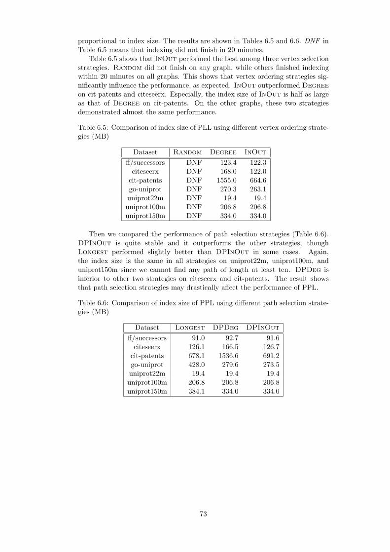
proportional to index size. The results are shown in Tables 6.5 and 6.6. DNF inTable 6.5 means that indexing did not finish in 20 minutes.

Table 6.5 shows that InOut performed the best among three vertex selectionstrategies. Random did not finish on any graph, while others finished indexingwithin 20 minutes on all graphs. This shows that vertex ordering strategies sig-nificantly influence the performance, as expected. InOut outperformed Degreeon cit-patents and citeseerx. Especially, the index size of InOut is half as largeas that of Degree on cit-patents. On the other graphs, these two strategiesdemonstrated almost the same performance.

Table 6.5: Comparison of index size of PLL using different vertex ordering strate-gies (MB)

Dataset Random Degree InOut

ff/successors DNF 123.4 122.3citeseerx DNF 168.0 122.0cit-patents DNF 1555.0 664.6go-uniprot DNF 270.3 263.1uniprot22m DNF 19.4 19.4uniprot100m DNF 206.8 206.8uniprot150m DNF 334.0 334.0

Then we compared the performance of path selection strategies (Table 6.6).DPInOut is quite stable and it outperforms the other strategies, thoughLongest performed slightly better than DPInOut in some cases. Again,the index size is the same in all strategies on uniprot22m, uniprot100m, anduniprot150m since we cannot find any path of length at least ten. DPDeg isinferior to other two strategies on citeseerx and cit-patents. The result showsthat path selection strategies may drastically affect the performance of PPL.

Table 6.6: Comparison of index size of PPL using different path selection strate-gies (MB)

Dataset Longest DPDeg DPInOut

ff/successors 91.0 92.7 91.6citeseerx 126.1 166.5 126.7cit-patents 678.1 1536.6 691.2go-uniprot 428.0 279.6 273.5uniprot22m 19.4 19.4 19.4uniprot100m 206.8 206.8 206.8uniprot150m 384.1 334.0 334.0

73

Chapter 7

Highway-based Labeling for Road Networks

Next, we deal with shortest-path and distance queries on road networks. As weexplained in Chapter 1, structural properties of road networks are quite differentfrom those of complex networks. Moreover, as road networks are weighted graphs,the bit-parallel labeling technique cannot be used. Therefore, we propose anothermethod named pruned highway labeling, which is tailored to road networks.

We first propose another indexing framework (i.e., index data structure andquery algorithm) named highway-based labeling framework (Section 7.1), whichis another extension of the 2-hop cover framework. Then, the overview of ourpruned highway labeling algorithm is presented (Section 7.2). Next, we presentthe detailed description of the algorithm (Section 7.3). Finally, results of ourexperimental evaluation is explained (Section 7.4).

7.1 Highway-based Labeling Framework

In this section, we propose a new labeling framework (i.e., data structure andquery algorithm) referred to as the highway-based labeling framework. We firstintroduce the notion of a highway decomposition and explain what we store forlabels (Section 7.1.1). This concept has some similarity to the decompositionused in Thorup [Tho04]. We then present our query algorithm (Section 7.1.2).

7.1.1 Highway Decomposition and Index Data Structure

First, we define a highway decomposition, which is a key for our proposed frame-work. In what follows, we identify a path with an ordered set of vertices.

Definition 7.1 (highway decomposition). A highway decomposition of a givengraph G is a family of ordered sets of vertices P = P1, P2, ..., PN such that,

1. Pi = (pi,1, pi,2, . . . , pi,li) is a shortest path between two vertices pi,1 and pi,li,

2. Pi ∩ Pj = ∅ for any i and j (i 6= j), and

3. P1 ∪ P2 ∪ . . . ∪ PN = V .

In Section 7.3 we will describe how to compute a highway decomposition ofa graph. In the following, we assume that we are given such a decomposition.In the highway-based labeling framework, a label L(v) for a vertex v is a set oftriples (i, d(pi,1, pi,j), d(v, pi,j)), that is, for each vertex v, we store an index i of

74

a path Pi, distance from the starting point pi,1 of the path to a vertex pi,j on thepath, and distance from the vertex v to the vertex pi,j

1.In the hub-based labeling framework (i.e., the 2-hop cover framework), a can-

didate for the distance between s and t are computed from pairs (v, d(s, v)) ∈ L(s)and (v, d(t, v)) ∈ L(t) for the same vertex v. On the other hand, in the highway-based labeling framework, we can compute a candidate for the distance betweens and t even for the case that the vertices stored in two triples are different.Indeed, suppose that the label L(s) contains a triple (i, d(pi,1, pi,j), d(s, pi,j))and the label L(t) contains a triple (i, d(pi,1, pi,k), d(t, pi,k)). Then we can ob-tain a candidate distance by looking at d(s, pi,j) + d(pi,j , pi,k) + d(pi,k, t) =d(s, pi,j) + |d(pi,1, pi,j) − d(pi,1, pi,k)| + d(pi,k, t). This observation is crucial inour experiment. It allows us to make the label for each vertex to be smaller size.This is a clear advantage of the highway-based labeling framework. In particular,a large part of distances between pairs of far vertices can be answered by storinga few distances to central paths in real road networks (e.g. highways).

7.1.2 Query Algorithm

For an s-t query, we search for the triples that minimize the candidate distance.That is, we define the answer to an s-t query using labels L as

Query(s, t, L)

= mind(s, pi,j) + d(pi,j , pi,k) + d(pi,k, t) |(i, d(pi,1, pi,j), d(s, pi,j)) ∈ L(s), (i, d(pi,1, pi,k), d(t, pi,k)) ∈ L(t).

The distance d(pi,j , pi,k) itself is not contained in labels L(s) and L(t), but canbe computed by using d(pi,1, pi,j) and d(pi,1, pi,k) as mentioned above.

Naively computing the function above takes Θ(|L(s)| |L(t)|) time, but we canobtain a linear-time algorithm based on the following lemma.

Lemma 7.1. There exist triples (i, d(pi,1, pi,j), d(s, pi,j)) ∈ L(s) and(i, d(pi,1, pi,k), d(t, pi,k)) ∈ L(t) that achieve the minimum candidate distanceand satisfy the following: for any vertex pi,l with min(j, k) < l < max(j, k),(i, d(pi,1, pi,l), d(s, pi,l)) 6∈ L(s) and (i, d(pi,1, pi,l), d(t, pi,l)) 6∈ L(t).

Proof. Let (i, d(pi,1, pi,j), d(s, pi,j)) ∈ L(s) and (i, d(pi,1, pi,k), d(t, pi,k)) ∈ L(t) betriples that minimize the candidate distance. Let us choose j, k with j < k suchthat k − j is as small as possible. Suppose there exists pi,l with j < l < ksuch that (i, d(pi,1, pi,l), d(s, pi,l)) ∈ L(s). Then the candidate distance computedfrom triples (i, d(pi,1, pi,l), d(s, pi,l)) and (i, d(pi,1, pi,k), d(t, pi,k)) must also be theminimum, because

d(s, pi,l) + d(pi,l, pi,k) + d(pi,k, t)

= d(s, pi,l) + d(pi,1, pi,k)− d(pi,1, pi,l) + d(pi,k, t)

= (d(s, pi,j) + d(pi,j , pi,l)) + d(pi,1, pi,k)

−(d(pi,1, pi,j) + d(pi,j , pi,l)) + d(pi,k, t)

= d(s, pi,j) + d(pi,1, pi,k)− d(pi,1, pi,j) + d(pi,k, t)

= d(s, pi,j) + d(pi,j , pi,k) + d(pi,k, t).

Note that Pi is a shortest path. This is a contradiction.1The label L(v) does not necessarily contain triples from all indexes i nor contains triples

for all the vertices on a path Pi, because in our preprocessing, we will reduce the total size oflabels L(v).

75

Therefore, like previous labeling methods, by sorting triples in labels withindexes and the distances from the starting point of the path in ascending orderbeforehand, we can answer an s-t query in O(|L(s)|+ |L(t)|) time using a merge-sort-like algorithm.

7.2 Pruned Highway Labeling

In this section we propose our label computation algorithm for highway-basedlabelings. Throughout this section, we assume that a highway decomposition Pis given. In Section 7.3, we will explain how to obtain such a decomposition.

7.2.1 Naive Highway Labeling

Before presenting our efficient preprocessing algorithm, we first give a naive algo-rithm to compute correct labels for the highway-based labeling framework. Westart with empty labels L0 (i.e., L0(v) = ∅ for each vertex v) and then constructnew labels Li+1 from Li iteratively. In order to construct the labels Li, we firstcopy the labels Li−1 to Li, and then conduct the Dijkstra search from each ver-tex pi,j on the path Pi and add the distance between vertices v and pi,j to thelabel Li(v). That is, Li(v) = Li−1(v) ∪ (i, d(pi,1, pi,j), d(v, pi,j)) for all pi,j ∈ Pi.After we conduct all Dijkstra searches, we obtain the labels L = LN . BecauseL(v) contains the distance from v to all vertices, the labels can answer correctdistances between v and any other vertex. Therefore we have the following.

Lemma 7.2. For any pair of vertices s and t, Query(s, t, L) = d(s, t).

7.2.2 Pruned Highway Labeling

We now explain our efficient algorithm for computing labels for the highway-basedlabeling framework named pruned highway labeling. This algorithm is based onthe pruned landmark labeling.

Similarly to the naive algorithm, we start with empty labels L′0 and then

construct new labels L′i+1 from L′

i iteratively. In order to construct the labelsL′i, we conduct the pruned Dijkstra search from all the vertices on the path Pi

simultaneously as described in Algorithm 7.1. When we visit a vertex v fromthe vertex pi,j with distance δ, if Query(v, pi,j , L

′i) is less than or equal to δ,

we prune the search. Otherwise, we add the triple (i, d(pi,1, pi,j), δ) to L′i(v) and

check edges from the vertex v. After we conduct the pruned Dijkstra searchesfrom all the paths, we obtain the labels L′ = L′

N for the highway-based labelingframework. We prove the correctness of our algorithm in Section 7.2.4, but inthe next subsection, we shall give intuition how our algorithm goes.

7.2.3 Example For Pruned Highway Labeling

Figure 7.1 illustrates examples for the pruned highway labeling. For simplicity,we assume that the length of all edges is 1.

First, we decompose the input graph. Suppose that we are given a highwaydecomposition P = P1, P2, P3, where P1 = 0, 1, 2, 3, 4, P2 = 5, 6, P3 =7, 8. Then we conduct the pruned Dijkstra search from the path P1 (Figure1a). A triple (1, 2, 1) is added to the label L′

1(5). However, a triple (1, 3, 2) is notadded to the label L′

1(5) because Query(5, 3, L′1) = d(5, 2) + d(2, 3) + d(3, 3) =

1 + 1 + 0 = 2. Therefore, the search from the vertex 3 is pruned. In the sameway, only one triple (1, 3, 1) is added to the label L′

1(6). On the other hand,

76

Algorithm 7.1 Pruned Dijkstra search from Pi to compute the labels L′i

procedure PrunedDijkstraSearch(G,Pi, L′i−1)

Q← an empty priority queuePush (0, pi,j , pi,j) onto Q for all pi,j ∈ Pi

L′i(v)← L′

i−1(v) for all v ∈ Vwhile Q is not empty do

Pop (δ, v, pi,j) from Qif Query(v, pi,j , L

′i) ≤ δ then

continueL′i(v)← L′

i(v) ∪ (i, d(pi,1, pi,j), δ)Push (δ + w(v, u), u, pi,j) onto Q for all (v, u) ∈ E

return L′i

Algorithm 7.2 Preprocessing by the pruned highway labeling

procedure Preprocess(G)L′0(v)← ∅ for all v ∈ V

P ← a highway decomposition of GN ← the size of Pfor i = 1 to N do

L′i ← PrunedDijkstraSearch(G,Pi, L

′i−1)

return L′N

two triples (1, 0, 1) and (1, 1, 1) are added to the label L′1(7) because we cannot

prune the search.Next, we conduct the pruned Dijkstra search from the path P2 (Figure 1b).

Because the search is pruned, no triples are added to labels L′2(2) nor L

′2(3) and

no other vertices are visited. Similarly, we conduct the pruned Dijkstra searchfrom the path P3 (Figure 1c).

For a query between vertices 6 and 7, we check the two labels L′(6) and L′(7).The triple (1, 3, 1) is contained in L′(6) and the triple (1, 0, 1) is contained inL′(7), so the distance computed by these triples is d(6, 3) + d(3, 0) + d(0, 7) =1+ 3+ 1 = 5. L′(7) also contains the triple (1, 1, 1). We can indeed get 4 as thedistance by using this triple. Although both labels L′(6) and L′(7) contain othertriples, these triples do not coincide to the index of the path. Therefore, we donot need to check these triples. As a result, Query(6, 7, L′) = 4.

7.2.4 Proof of Correctness

In this subsection, we prove the correctness of the pruning. Specifically, we provethat the distance computed by using labels L′ from the pruned highway labelingis equal to the distance computed by using labels L from the naive highwaylabeling.

Theorem 7.1. For any pair of vertices s and t, Query(s, t, L′) =Query(s, t, L).

Proof. For vertices s and t, let i be the index such that Query(s, t, Li′) 6= d(s, t)for any i′ < i andQuery(s, t, Li) = d(s, t). Then there exist vertices pi,j , pi,k ∈ Pi

that satisfy d(s, t) = d(s, pi,j) + d(pi,j , pi,k) + d(pi,k, t). Among others, we choosea pair (j, k) such that no vertices on the shortest path between s and pi,j orbetween pi,k and t are on the path Pi. Suppose that for some i′ < i, a vertex pi′,j′

77

0 13

5

6

4

8

2

7

(a) Pruned Dijkstrasearch from the path P1

0 13

5

6

4

8

2

7

(b) Pruned Dijkstrasearch from the path P2

0 13

5

6

4

8

2

7

(c) Pruned Dijkstrasearch from the path P3

Figure 7.1: Examples for the pruned highway labeling. Pink vertices are on thestarting path Pi, blue vertices are visited and added to some labels, gray verticesare already used as the starting points of the previous searches, orange verticesare visited but pruned, and white vertices are not visited.

on the path Pi′ is on a shortest path between s and pi,j . Then the label L(s)contains the triple (i′, d(pi′,1, pi′,j′), d(s, pi′,j′)) and the label L(t) contains thetriple (i′, d(pi′,1, pi′,j′), d(t, pi′,j′)), and therefore Query(s, t, Li′) = d(s, t) holds,which is a contradiction to the choice of i. Therefore any path Pi′ with i′ < icontains no vertices on the shortest paths between s and pi,j . Thus the searchfrom pi,j to s is not pruned and the triple (i, d(pi,1, pi,j), d(s, pi,j)) is added to thelabel L′(s). In the same way, the triple (i, d(pi,1, pi,k), d(t, pi,k)) is added to thelabel L′(t). As a result, Query(s, t, L′) = Query(s, t, L) holds.

From this theorem, we can answer a query for any pair of vertices correctlyby using labels computed by the pruned highway labeling.

Corollary 7.1. Let L′ be the labels computed by the pruned highway labeling.Then for any pair of vertices s and t,

Query(s, t, L′) = d(s, t).

7.3 Detailed Algorithm Description

7.3.1 Heuristic Highway Decomposition

Until this point, we assumed that a highway decomposition is already given, andthen we conduct the first pruned Dijkstra search. We now show how to constructa highway decomposition and labeling simultaneously. Specifically, we choose apath Pi from remaining vertices just before conducting the i-th pruned Dijkstrasearch. In the pruned landmark labeling algorithm, the order of vertices to startBFSs is crucial to achieve small labels. Similarly, in our method, the order ofpaths Pi in a highway decomposition is important, and this allows us to achievesmall label sizes.

At a high level, we want to choose a path that hits many shortest paths atthe early stage of Dijkstra search, because this would allow us to prune futureDijkstra searches. In what follows, we propose strategies for selecting such a goodpath.

First, we focus on the speed of an edge (i.e., the geometrical length dividedby the travel time). In the real life, we tend to use fast highways when we travellong distance. Therefore, we may assume that the vertices connected to fast edgestend to be passed by many shortest paths. For this reason, we group vertices into

78

several levels according to the speed of their connected edges. We assign verticesconnected to faster edges to higher levels and then we choose a path consistingof the highest level vertices. When the number of vertices in the highest levelis fewer than some threshold, we mix unused vertices in the highest level withvertices in the second highest level to make it possible to select a path of enoughlength.

We now describe how to choose a path from the highest level vertices. Becausethe selected path must be a shortest path between two vertices, we first computethe shortest path tree from a randomly selected root vertex, and then pick a pathbetween the root vertex and another vertex in the shortest path tree. The moredescendants a vertex has in the shortest path tree, the more shortest paths on thetree hit the vertex. Therefore, in order to select a path that hits many shortestpaths, we choose the path by starting from the root vertex and iteratively pick achild with the largest number of descendants.

Finally, we describe our technique to skip unimportant vertices. Suppose thata vertex v on the selected path hits many shortest paths, but most of them alsocontain another vertex w on the selected path. In this case, even if we skip thevertex v while keeping the vertex w, most of the future searches that will bepruned by v are still pruned by w. Thus we skip such unimportant vertices fromthe selected path. Suppose that we chose a vertex v on the shortest path tree, andthen choose its child w. If the difference between the number of descendants of vand w is small, most of the shortest paths on the tree that contain v also containw, and therefore we skip v. This does not affect the correctness of the algorithmbecause this operation corresponds to add shortcut edges across skipped vertices.

In our implementation used in the experiments, we group vertices into fourlevels and we skip a vertex v when the difference between the number of descen-dants of vertices v and its child w is smaller than five percents.

7.3.2 Storing Labels

To make highway-based labelings more practical, we describe the efficientway to store labels in this subsection. The label L(v) is a set of triples(i, d(pi,1, pi,j), d(v, pi,j)), where i is an index of a path. The distance informa-tion in the label is used in the query only when the indexes of the paths aresame in two triples. Therefore, storing the index information and the distanceinformation separately makes the query time faster because we can avoid cachemisses. For a single path, multiple triples may be stored to a vertex. Therefore,by storing pairs of an index and the number of triples for the index, we can re-duce the space usage. Moreover, this also makes the query time faster becausewe can reduce unnecessary comparisons when the indexes do not match in twotriples. For more efficient implementation, we use pointer arithmetic and alignarrays storing labels to cache line.

7.3.3 Contraction Technique

Additionally, to further improve the performance, we introduce a new techniquecalled the contraction technique. First, we consider a vertex v of degree one.Any shortest path from v to another vertex passes through its adjacent vertex x.Moreover, the vertex v is never contained in shortest paths between other vertices.Therefore, we can remove the vertex v from the graph in the preprocessing. Wecan correctly answer the query between the vertex v and another vertex u byreferring the label L(x) and adding the length w(v, x), that is, Query(v, u, L) =

79

Query(x, u, L) + w(v, x).Next, we consider a vertex v of degree larger than one. In this case, the

vertex v may be contained in a shortest path between other vertices. Therefore,we need to add some shortcut edges before removing the vertex v to preservethe distances. We can correctly answer the distance between v and anothervertex u by evaluating the distances from all the neighbors of v to u, that is,Query(v, u, L) = min(v,x)∈E(G)Query(x, u, L) + w(v, x). However, the largerthe degree limit is, the slower query time becomes due to the number of neighborsto check. In our experiments, we only set the degree limit to be at most three.

7.4 Experimental Evaluation

7.4.1 Setup

Environment

We conducted experiments on a Linux server with Intel Xeon X5675 processor(3.06 GHz) and 288 GB for main memory. We implemented the proposed methodin C++ and compiled it with the GNU C++ compiler 4.4.6 using optimizationlevel 3. We did not parallelize the preprocessing and queries and used one core.We evaluate query time as the average time for 1,000,000 random queries.

Datasets

We used two popular graph instances from 9th DIMACS Implementation Chal-lenge [DGJ09]. One is a road network of USA that has about 24 million verticesand 58 million edges. The other is a road network of Western Europe by PTVAG with about 18 million vertices and 42 million edges. In both instances, weuse travel times as the length of edges and treat a graph as an undirected graph.

7.4.2 Performance Comparison

First, we compare the proposed method with several previous methods withregard to preprocessing time, space usage and query time (Table 7.1). Theproposed method is set to use the contraction technique for vertices of degreeone. We compare the proposed method with the following five previous methods:contraction hierarchies (CH) [GSSD08], transit node routing (TNR) [BFM+07],combination of TNR and arc flags (TNR+AF) [BDS+10], hub-based labeling(HL) [ADGW11, ADGW12], and hub label compression (HLC) [DGW13]. ForHL, we used four variants: HL local [ADGW11], HL global [ADGW11], HL-15 local [ADGW12] and HL-∞ global [ADGW12]. All these methods are alsoimplemented in C++. CH, TNR and TNR+AF were evaluated on a ma-chine with an AMD Opteron 270 processor (2.0 GHz) [BDS+10], and HL andHLC were evaluated on a machine with two Intel Xeon X5680 processors (3.33GHz) [ADGW11,ADGW12,DGW13]. The preprocessing is parallelized for onlyHL but not parallelized for other methods including our method. Queries are notparallelized for all methods.

Preprocessing Time

We would like to emphasize our big improvement in preprocessing time. Thepreprocessing time for the proposed method is much faster than previous labelingmethods. Although it seems that HL-15 local is faster than our method, let us

80

Table 7.1: Comparison of the performance between pruned highway labeling andprevious methods. HL is parallelized to use 12 cores in preprocessing and allother methods are not parallelized.

USA EuropePrep. Space Query Prep. Space Query

Method [h:m] [GB] [ns] [h:m] [GB] [ns]

PHL-1 (This work) 0:29 16.4 941 0:34 14.9 1039

CH [BDS+10] 0:27 0.5 130000 0:25 0.4 180000TNR [BDS+10] 1:30 5.4 3000 1:52 3.7 3400TNR+AF [BDS+10] 2:37 6.3 1700 3:49 5.7 1900HL local [ADGW11] 2:24 22.7 627 2:39 20.1 572HL global [ADGW11] 2:35 25.4 266 2:45 21.3 276HL-15 local [ADGW12] - - - 0:05 18.8 556HL-∞ global [ADGW12] - - - 6:12 17.7 254HLC-15 [DGW13] 0:53 2.9 2486 0:50 1.8 2554

observe that its preprocessing is parallelized to use 12 cores. This improvementshows the efficiency of pruned labeling.

Space Usage

The space consumption for our method is also smaller than HL. While this maybe still not very compact, in the situations when space consumption is severe,we can greatly reduce the space usage with help of the contraction technique, atthe cost of a little slower query time, as discussed in Section 7.4.3. Therefore, itwould be not a big problem.

Query Time

With regard to query time, although our method is a bit slower than HL, it isstill sufficiently fast and around 1 µs on average. This shows the efficiency of thehighway-based labeling as a labeling framework.

7.4.3 Analysis

Contraction Technique

Table 7.2 lists the performance of our method with different contraction level.The contraction level denotes the limit of the degree of vertices to remove. Thatis, if the level is 2, we remove vertices of degree no larger than 2. Setting thecontraction level zero means we do not use the contraction technique at all.

Even without the contraction technique, our preprocessing is much fasterthan previous labeling methods. However, by applying the contraction tech-nique, preprocessing time becomes even faster. In particular, it takes only aboutten minutes with contraction level three. This is because the input graph sizeis fairly reduced by this contraction. Moreover, the space usage gets smallerthan five gigabytes with contraction level three, while the query time is not veryslower. Although the higher the level is, the slower the query time becomes, it issufficiently fast. Therefore, the contraction technique is highly useful.

Pruning

Figure 7.2a illustrates the number of triples added to labels in each pruned Di-jkstra search and Figure 7.2b illustrates the cumulative distribution of it. We

81

Table 7.2: Comparison of the performance by the contraction technique. Thecontraction level indicates the degree of removed vertices.

USA EuropePreprocessing Space Query Preprocessing Space Query

Contraction level [h:m] [GB] [ns] [h:m] [GB] [ns]0 0:38 19.8 906 0:50 20.2 10801 0:29 16.4 941 0:34 14.9 10392 0:11 6.4 1793 0:22 8.5 20113 0:07 4.1 2970 0:11 4.6 3344

can confirm big effect of pruning from these figures. From Figure 7.2a, we ob-serve that the number of triples added to labels in each pruned Dijkstra searchdecreases dramatically. In consequence, as Figure 7.2b shows, most triples areadded at the beginning.

Figure 7.3a reports the average number of common paths in labels of twovertices against Dijkstra rank of them. We used labels constructed without thecontraction technique and computed the average on 10,000 pairs of vertices foreach rank. We observe that the number of common paths decreases gradually asthe two vertices get far. This indicates that our preprocessing algorithm success-fully separates input graphs by shortest paths.

100

101

102

103

104

105

106

107

108

109

100

101

102

103

104

105

106

107

Nu

mb

er

of

Trip

les

i-th Dijkstra search

USAEurope

(a) Number of triples added in each pruned Dijkstra search.

0

0.1

0.2

0.3

0.4

0.5

0.6

0.7

0.8

0.9

1

100

101

102

103

104

105

106

107

Cu

mu

lative

Pe

rce

ntile

i-th Dijkstra search

USAEurope

(b) Cumulative distribution of the number of triples added ineach pruned Dijkstra search.

Figure 7.2: Effect of pruning.

82

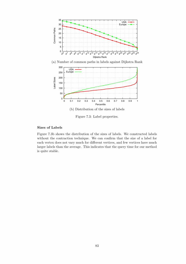
0

5

10

15

20

25

30

35

26

27

28

29

210

211

212

213

214

215

216

217

218

219

220

221

222

223

224

Co

mm

on

Pa

ths

Dijkstra Rank

USAEurope

(a) Number of common paths in labels against Dijkstra Rank

0

50

100

150

200

250

300

0 0.1 0.2 0.3 0.4 0.5 0.6 0.7 0.8 0.9 1

La

be

l S

ize

s

Percentile

USAEurope

(b) Distribution of the sizes of labels

Figure 7.3: Label properties.

Sizes of Labels

Figure 7.3b shows the distribution of the sizes of labels. We constructed labelswithout the contraction technique. We can confirm that the size of a label foreach vertex does not vary much for different vertices, and few vertices have muchlarger labels than the average. This indicates that the query time for our methodis quite stable.

83

Chapter 8

Historical Labeling for Evolving Complex

Networks

When analyzing historical networks, for which timestamps of vertices and edgesare also available, in addition to the latest snapshot, the shortest paths anddistances on previous snapshots or transition of them by time are also of interest.In this chapter, we call such queries about previous snapshots historical queries.We study indexing methods for such kinds of historical queries (Figure 8.1). Inparticular, we deal with the following two kinds of queries: a snapshot query asksthe shortest path or distance on a specified previous snapshot, and a change-pointquery asks all the moments when the distance between two vertices has changed.

Tim

e

Index

Query: transition of distance

Time

Distance

Figure 8.1: An illustration of indexing methods for historical queries.

We first design an indexing method based on pruned landmark labeling forthese kinds of queries (Section 8.1). Second, we present the result of experimentalevaluation (Section 8.2). Finally, the usefulness of these new kinds of historicalqueries is demonstrated via application to evolving network analysis (Section 8.3).

Formal Problem Definition

In this chapter, we study indexing methods that, given a time series of a evolvinggraph (i.e., a graph with edge time stamps), construct an index to quickly answerthe following queries.

Problem 8.1 (Historical Snapshot Distance Query).Given: Two query vertices s, t and time τ .

84

Answer: Distance dτ (s, t).

Problem 8.2 (Historical Distance Change-point Query).Given: Two query vertices s, t.Answer: Set C(s, t) = (τ1, δ1), (τ2, δ2), . . . where (τi, δi) ∈ C(s, t) if and onlyif δi = dτi(s, t) 6= dτi−1(s, t).

8.1 Historical Pruned Landmark Labeling

In this section, we propose a new indexing scheme referred to as historical prunedlandmark labeling to efficiently process historical queries defined above. Unlikeour first method for contemporary queries, as there is no previous work on thesequeries, we start from designing a new index framework (i.e., data structureand query algorithms), named historical 2-hop cover, in Section 8.1.1. Then,we propose an offline indexing algorithm that constructs an index from a storedhistorical graph in Section 8.1.2. Since it is more involved than that for stan-dard contemporary queries, we explain our indexing algorithm with three steps:we start from an algorithm based on dynamic programming, next we turn thealgorithm into a BFS-like algorithm, and then introduce pruning to the algo-rithm. Finally, we present an online incremental update algorithm for onlinegraph changes in Section 8.1.3.

8.1.1 Historical 2-Hop Cover Framework

First, we propose a new indexing framework (i.e., data structure and query al-gorithms) referred to as the historical 2-hop cover framework. Since there is noprevious work on these queries, it is the first framework for historical distancequeries. The main technical challenge here is to design (almost) linear-time queryalgorithms for both kinds of historical queries.

Data Structure

For each vertex v, we store a label L(v). Label L(v) is a set of triples (u, τ, δuv),where u is a vertex, τ describes time, and δuv = dτ (u, v). Due to Lemma 4.2,(u, τ, δuv) ∈ L(v) also indicates dτ ′(u, v) ≤ δuv for τ ′ ≥ τ .

As with the normal 2-hop cover framework, we store triples in a label in theascending order of the IDs of destination vertices. In addition, we sort triples thatshare the same destination vertex in ascending order of distance (i.e. descendingorder of time).

Answering Snapshot Queries

A snapshot query between a pair of vertices s and t at time τ can be answered inO(|L(s)|+ |L(t)|) time. Though we basically conduct a merge-sort-like algorithmas with normal 2-hop cover, there are several differences. First, we need to ignorelabel entries with time later than τ . In addition, to handle triples in a label thatshare the same destination vertex, among them we only see the newest label entrywith time earlier than or equal to τ . That is, if (ui, τi, δi) and (ui+1, τi+1, δi+1)are consecutive labels in L(s) where ui = ui+1 and τ ≥ τi > τi+1, then we ignorethe second label since δi ≤ δi+1 from Lemma 4.2.

85

Answering Change-point Queries

Answering a change-point query between vertices s and t is a little more involved,but can be done in O(l log l) time, where l = |L(s)| + |L(t)|. First, we conducta merge-sort-like algorithm to enumerate candidates of distance change-points.From pairs of triples (u, τs, δs) ∈ L(s) and (u, τt, δt) ∈ L(t), we enumerate pairs(τ, δ) = (max τs, τt , δs + δt), which indicates dτ (s, t) ≤ δ. Then, we sort thesepairs by time τ . Finally, we remove unnecessary pairs. That is, if (τi, δi) and(τi+1, δi+1) are consecutive pairs, where τi ≤ τi+1 and δi ≤ δi+1, then we removethe second pair.

Again, the remaining issue is to handle triples in a label that share the samedestination vertex. If we check every pair of these triples, in the worst case, itwould take quadratic time. However, for these triples, we can also apply a merge-sort-like scan algorithm by considering time of these triples. The algorithm isdescribed in Algorithm 8.1, where v(t) = v, τ(t) = τ and δ(t) = δ for triplet = (v, τ, δ). In total, the first step and the final step can be done in linear time,and the time complexity is dominated by sorting.

Algorithm 8.1 Answer change-point query (s, t)

1: procedure QueryChangePoints(s, t, L)2: is, it ← 03: C ← an empty array4: while is < |L[s]| and it < |L[t]| do5: if v(L[s][is]) < v(L[t][it]) then6: is ← is + 17: else if v(L[s][is]) > v(L[t][it]) then8: it ← it + 19: else

10: τ ← max τ(L[s][is]), τ(L[t][it])11: δ ← δ(L[s][is]) + δ(L[t][it])12: Push (τ, δ) to C13: if v(L[t][it + 1]) 6= v(L[t][it]) then14: is ← is + 115: else if v(L[s][is + 1]) 6= v(L[s][is]) then16: it ← it + 117: else if τ(L[s][is] > τ(L[t][it])) then18: is ← is + 119: else20: it ← it + 1

21: Sort pairs in C by time.22: Filter out unnecessary pairs from C.23: return C

8.1.2 Offline Indexing Algorithm

For presenting the indexing algorithm for contemporary queries, we first de-scribed a naive labeling algorithm without pruning, then we introduced pruningto present the indexing algorithm. However, designing an algorithm for historicalqueries is more challenging since, while the naive labeling algorithm was obviousfor contemporary queries, this time, even the naive labeling algorithm withoutpruning is not trivial for historical 2-hop cover. Therefore, we explain our index-

86

ing algorithm with three steps: we start from an algorithm based on dynamicprogramming, next we turn the algorithm into a BFS-like algorithm, and finallyintroduce pruning to the algorithm to obtain our indexing algorithm.

Dynamic Programming

As usual, we start from an empty index L0 and construct index Lk from Lk−1 byadding triples whose destination vertex is vk. Let D be the maximum distance toa connected vertex from vk regarding all the snapshots. Let T be a (D+1)× |V |table. We conduct dynamic programming on the table T so that each cell T [δ][u]denotes the earliest time τ with dτ (vk, u) ≤ δ. First, we fill the cells with distancezero as T [0][vk] = 0 and T [0][u] =∞ for any u 6= vk. Then, we compute the valuesof cells with distance δ > 0 from smaller δ by the following recurrence relation:

T [δ][u] = minw∈N(u)

max T [δ − 1][w], t(w, u) ,

for any u 6= vk and T [δ][vk] = 0.

Lemma 8.1. Each cell T [δ][u] denotes the earliest time τ with dτ (vk, u) ≤ δ.

This lemma can be proved by mathematical induction on δ. After computingthe table, we add triple (vk, δ, τ) to label Lk(u) where τ = T [δ][u] if T [δ][u] 6=∞and δ = 0 or T [δ][u] < T [δ − 1][u].

Historical Naive Landmark Labeling

While the algorithm above computes the correct index, it takes Θ(D |E|) timeand Θ(D |V |) space. In this subsection, we reduce the time and space complexityby skipping unnecessary computations. Again, we suppose we are to constructindex Lk from Lk−1 by adding triples whose destination vertex is vk.

The key insight here is the following simple fact. For simplicity, we defineT [−1][u] = ∞ for any vertex u in the following. For any vertex u and δ ≥ 0, ifT [δ − 1][w] = T [δ][w] for all w ∈ N(u), then T [δ + 1][u] = T [δ][u]. Therefore, weavoid vainly computing values of such cells as follows. For each distance δ ≥ 0and vertex u, we initially set T [δ + 1][u] = T [δ][u]. Then, we only check edges(w, u) incident to vertex w with T [δ− 1][w] 6= T [δ][w], and update T [δ+1][u] bymax T [δ][w], t(w, u) if it is smaller than the current value.

This can be efficiently achieved by managing vertices with queues. Weprepare two queues, Q and Q′, where initially Q contains vk and Q′ is empty.For each distance δ ≥ 0, supposing that Q contains vertices w with T [δ− 1][w] 6=T [δ][w], we check edges incident to each vertex w ∈ Q and create Q′ for the nextdistance δ + 1. If we obtain T [δ + 1][u] 6= T [δ][u] and u 6∈ Q′, we push u to Q′.Finally, before incrementing δ, we swap Q and Q′, and clear Q′. Note that, thealgorithm now behaves quite similarly to BFSs, although it may visit a vertexmore than once. We also add triple (vk, T [δ][u], δ) to label L(u) when we drawvertex u from Q.

However, even using queues, it still takes Ω(D |V |) time and Θ(D |V |) spacedue to the two-dimensional table. Thus, instead of straightforwardly using a two-dimensional table, we use two one-dimensional arrays with length O(|V |), andavoid full initialization for each distance δ. Consequently, conducting queue-baseddynamic programming and avoiding Θ(|V |) time initialization for each step, thetotal time complexity becomes O(m′), where m′ is the number of traversed edgesincluding duplications. Also note that, by using queues, we do not need to obtainthe maximum distance D beforehand, as it suffices to stop when the queues getempty.

87

Algorithm 8.2 Pruned BFS from vk ∈ V to create index L′k for historical

queries.

1: procedure PrunedBFS(G, vk, L′k−1)

2: L′k[v]← L′

k−1[v] for all v ∈ V (G).3: Q← a queue with only one element vk.4: T [vk]← 0 and T [v]←∞ for all v ∈ V (G) \ vk.5: T ′[v]←∞ for all v ∈ V (G).6: for all δ = 0, 1, . . . until Q gets empty do7: Q′ ← an empty queue.8: for all u ∈ Q do9: if QuerySnapshot(vk, u, T [u], L

′k−1) ≤ δ then

10: continue11: L′

k[u]← L′k[u] ∪ (vk, T [u], δ)

12: for all w ∈ NG(v) do13: τ ′ = max T [u], t(u,w)14: if τ ′ < T ′[w] and τ ′ < T [w] then15: if T ′[w] =∞ then16: Enqueue w onto Q′.

17: T ′[w]← τ ′.

18: T [u]← T ′[u], T ′[u]←∞ for all u ∈ Q′.19: Q← Q′.

20: return L′k

Historical Pruned Landmark Labeling

We finally introduce pruning to the previous algorithm to obtain our indexingalgorithm. Suppose we have started with an empty index L′

0 and we are con-structing index L′

k from L′k−1 and the result of the k-th pruned BFS from vk.

Along with the labeling algorithm for contemporary queries, after drawing vertexu from the queue Q, we issue a query between vk and u, and if the distance is atmost δ, we prune vertex u. The difference from the algorithm for contemporaryqueries here is that we issue a snapshot query with regard to time T0[u]. Thetotal algorithm is described as Algorithm 8.2.

The correctness of this algorithm is not obvious, but can be proved as theexactly same way as the correctness of the pruned landmark labeling algorithmfor contemporary queries.

Theorem 8.1. For any pair of vertices s, t and i, τ ≥ 0,QuerySnapshot(s, t, τ, Li) = QuerySnapshot(s, t, τ, L′

i).

Corollary 8.1. For any pair of vertices s and t and τ ≥ 0,QuerySnapshot(s, t, τ, L′

n) = dτ (s, t).

Corollary 8.2. For any pair of vertices s and t, (τ, δ) ∈QueryChangePoints(s, t, L′

n) if and only if dτi−1(s, t) 6= dτi(s, t) = δ.

By the same discussion as the standard pruned labeling algorithm, the timecomplexity is roughly estimated as O(ml + n2l) time. As with the standardalgorithms for contemporary queries, to exploit structures of real networks, weadopt the same vertex ordering strategies (i.e., we order vertices from those withhigher degree in the final snapshot).

88

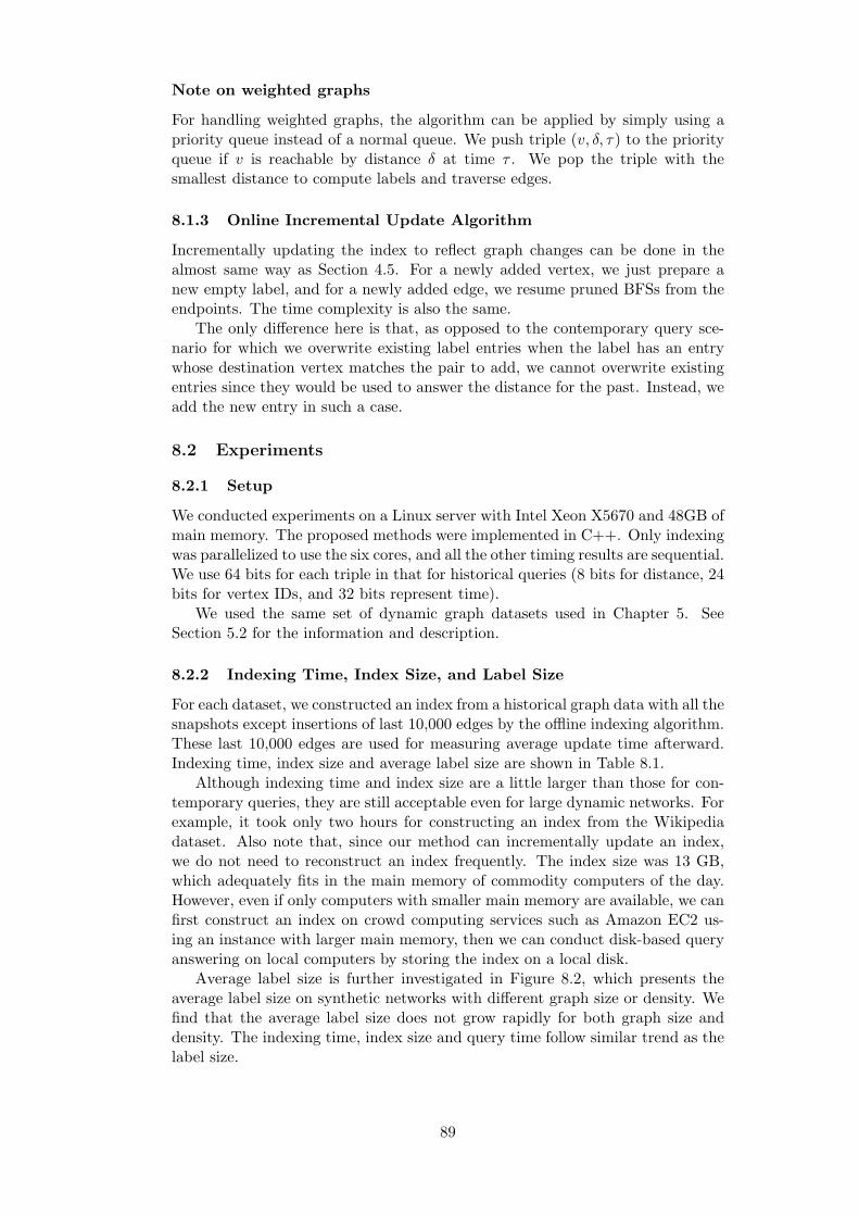
Note on weighted graphs

For handling weighted graphs, the algorithm can be applied by simply using apriority queue instead of a normal queue. We push triple (v, δ, τ) to the priorityqueue if v is reachable by distance δ at time τ . We pop the triple with thesmallest distance to compute labels and traverse edges.

8.1.3 Online Incremental Update Algorithm

Incrementally updating the index to reflect graph changes can be done in thealmost same way as Section 4.5. For a newly added vertex, we just prepare anew empty label, and for a newly added edge, we resume pruned BFSs from theendpoints. The time complexity is also the same.

The only difference here is that, as opposed to the contemporary query sce-nario for which we overwrite existing label entries when the label has an entrywhose destination vertex matches the pair to add, we cannot overwrite existingentries since they would be used to answer the distance for the past. Instead, weadd the new entry in such a case.

8.2 Experiments

8.2.1 Setup

We conducted experiments on a Linux server with Intel Xeon X5670 and 48GB ofmain memory. The proposed methods were implemented in C++. Only indexingwas parallelized to use the six cores, and all the other timing results are sequential.We use 64 bits for each triple in that for historical queries (8 bits for distance, 24bits for vertex IDs, and 32 bits represent time).

We used the same set of dynamic graph datasets used in Chapter 5. SeeSection 5.2 for the information and description.

8.2.2 Indexing Time, Index Size, and Label Size

For each dataset, we constructed an index from a historical graph data with all thesnapshots except insertions of last 10,000 edges by the offline indexing algorithm.These last 10,000 edges are used for measuring average update time afterward.Indexing time, index size and average label size are shown in Table 8.1.

Although indexing time and index size are a little larger than those for con-temporary queries, they are still acceptable even for large dynamic networks. Forexample, it took only two hours for constructing an index from the Wikipediadataset. Also note that, since our method can incrementally update an index,we do not need to reconstruct an index frequently. The index size was 13 GB,which adequately fits in the main memory of commodity computers of the day.However, even if only computers with smaller main memory are available, we canfirst construct an index on crowd computing services such as Amazon EC2 us-ing an instance with larger main memory, then we can conduct disk-based queryanswering on local computers by storing the index on a local disk.

Average label size is further investigated in Figure 8.2, which presents theaverage label size on synthetic networks with different graph size or density. Wefind that the average label size does not grow rapidly for both graph size anddensity. The indexing time, index size and query time follow similar trend as thelabel size.

89

100

101

102

103

215

216

217

218

219

220

Ave

rag

e la

be

l siz

e

Number of vertices

DMSHyperbolicForestFire

(a) Varying graph size

100

101

102

103

4 8 16 32 64 128

Ave

rag

e la

be

l siz

e

Density

DMSHyperbolic

(b) Varying density

Figure 8.2: Label size for historical queries on synthetic networks with differentsize and density.

8.2.3 Query Time

Average query time reported in Table 8.1 is measured by 1,000,000 randomqueries after reflecting all the dynamic updates. As a baseline for snapshotqueries, we also report the average time to evaluate a snapshot query by a BFSfor 1,000 random queries. As a baseline for change-point queries, we suppose anaive method that conducts a BFS for each snapshot. Since this baseline methodtakes too long query time, we estimated the average query time by the productof the average snapshot-query time and the number of snapshots. For both snap-shot queries and change-point queries, the query time of our method for historicalqueries is also generally microseconds and orders of magnitude faster than thebaselines.

8.2.4 Update Time and Label Increase

Average update time listed in Table 8.1 is measured by inserting the last 10,000edges of each dataset. As with the method for contemporary queries, this methodfor historical queries also handles each update in milliseconds. Moreover, asaverage label increase in Table 8.1 is small, we can confirm that the label sizegrows slowly.

90

Tab

le8.1:

Experim

entalresultsofourmethodforhistoricalqueriesagainst

real-worldandsynthetic

networks.

Dataset

HistoricalPruned

Landmark

Labeling(T

his

work)

BFS

Dataset

Indexing

Index

Snapshot

Change-point

Update

Label

Label

Snapshot

Chan

ge-point

time

size

querytime

querytime

time

size

increase

querytime

querytime

Epinions

23.1

s23

6MB

2.7

µs

4.6

µs

0.3

ms

234.2

2.6×

10−4

6.2

ms

2593

sEnron

5.4s

86MB

1.6

µs

3.0

µs

0.2

ms

128.5

4.0×

10−4

5.3

ms

3041

sP2P

2596

.4s

9.7GB

12.4

µs

22.0

µs

10.7

ms

1227.9

2.7×

10−4

79.5

ms

>1d

ayYouTube

1281

.8s

9.1GB

4.5

µs

8.1

µs

2.1

ms

374.7

4.0×

10−5

177.5

ms

>1d

ayWikipedia

5165

.9s

13.0

GB

9.8

µs

12.7

µs

8.3

ms

919.5

3.0×

10−5

413.3

ms

>1d

ay

DMS

920.0s

3.8GB

4.0

µs

5.6

µs

1.0

ms

481.1

8.6×

10−5

126.4

ms

>1d

ayHyperbolic

24.7

s19

5MB

0.5

µs

0.7

µs

0.1

ms

23.9

2.9×

10−6

86.2

ms

>1d

ayForestfire

1056

.3s

6.5GB

8.2

µs

12.8

µs

3.9

ms

835.9

3.6×

10−4

91.4

ms

>1d

ay

91

8.3 Application to Evolving Network Analysis

In this section, we demonstrate the usefulness of our historical indexing methodfor evolving network analysis. The proposed method enables quick and fine-grind temporal analysis of large-scale dynamic networks. For example, with ourindex, users can instantly and interactively check the transition of various featuresrelated to distances, which has never been available at all without our index.

We see by the case study in Section 8.3.1 that transitions of distance andshortest-path themselves are useful and of interest. Furthermore, based on ourmethod, we see that we can also efficiently compute the transition of the followingkinds of network features in the following sections.

8.3.1 Ego Network Analysis

Figure 8.3 illustrates an example of analysis on a real-world Facebook sub-graph [VMCG09] based on historical change-point queries. Figure 8.3a depictsan ego network, i.e., the induced subgraph of a center vertex and its neighbors,where the center vertex is the gray one. From the figure, we can observe thatthere are two clusters on the left and right of the center vertex. Figure 8.3bshows the transition of the distances between the center vertex and its neighbors,where the colors of the lines correspond to those of the vertices in Figure 8.3a.We can confirm that the time periods of the appearance of the friendship linksare different between the two clusters. Moreover, we find that the two clustershappened quite differently. That is, while the left cluster gradually approachedthe center vertex, the right cluster became neighbors almost instantly.

(a) An ego network

1

2

3

4

5

6

7

8

9

Time

Dis

tanc

e

(b) Distances to the neighbors

Figure 8.3: An example of social network analysis on a dynamic Facebook sub-graph [VMCG09] using our method for historical shortest-path distance queries.

8.3.2 Average Distance and Effective Diameter

Distance distribution is one of the most important features of networks, and thetransition of distance distribution of dynamic networks is of strong interest to thedata mining and social network analysis community [LKF07]. Though calculatingdistance distribution of one graph is already too costly, to obtain the transitionof it, we need to do so for many snapshots of graphs, which would be impossi-ble for large historical networks. Using our historical indexing method, however,we can estimate the transition just by evaluating random change-point querieswith regard to a set of randomly sampled pairs of vertices. To demonstrate theeffectiveness of our method, we computed the transition of the average distance

92

2

2.5

3

3.5

4

4.5

5

5.5

6

Ave

rag

e d

ista

nce

Snapshot

EnronEpinions

P2P

YouTubeWikipedia

DMS

Forestfire

(a) Average distance

4

6

8

10

12

14

Eff

ective

dia

me

ter

Snapshot

EnronEpinions

P2P

YouTubeWikipedia

DMS

Forestfire

(b) Effective diameter

Figure 8.4: Transition of average distance and effective diameter.

0.06

0.065

0.07

0.075

0.08

0.085

0.09

0.095

0.1

Clo

se

ne

ss C

en

tra

lity

Snapshot

(a) Enron

0.06

0.07

0.08

0.09

0.1

0.11

0.12

0.13

Clo

se

ne

ss C

en

tra

lity

Snapshot

(b) Epinions

Figure 8.5: Transition of the closeness centrality of some popular vertices.

between pairs and the effective diameter (the 90th percentile distance) of vari-ous networks (Figure 8.4). We can observe that average distance decreases overtime, which confirms the claim of [LKF07], but the effective diameter sometimesincreases.

8.3.3 Closeness Centrality

Closeness centrality is one of the most popular network centralities defined onvertices. There are several different definitions, but all of them are based ondistances to other vertices, and thus they can be efficiently estimated by randomchange-point queries. Here, we adopt the definition that defines the closenesscentrality of vertex v as 1

|V |∑

u∈V 2−d(v,u). We picked up several vertices of highcloseness centralities from Enron and Epinions and computed the transition oftheir closeness centralities by the proposed method (Figure 8.5). We can see thatthe closeness centrality sometimes drastically increases as some moment.

8.3.4 Temporal Hop Plot

To study distance distribution in depth, the (temporal) hop plot, which is thetransition of the fraction of pairs within a fixed distance, is also used. We canapproximate the hop plot by evaluating change-point queries with regard to aset of randomly sampled pairs of vertices. In Figure 8.6, we illustrate the hopplot of YouTube and Wikipedia for various distances. We observe that it tendsto increase over time, as expected from the fact that average distance decreasesover time.

93

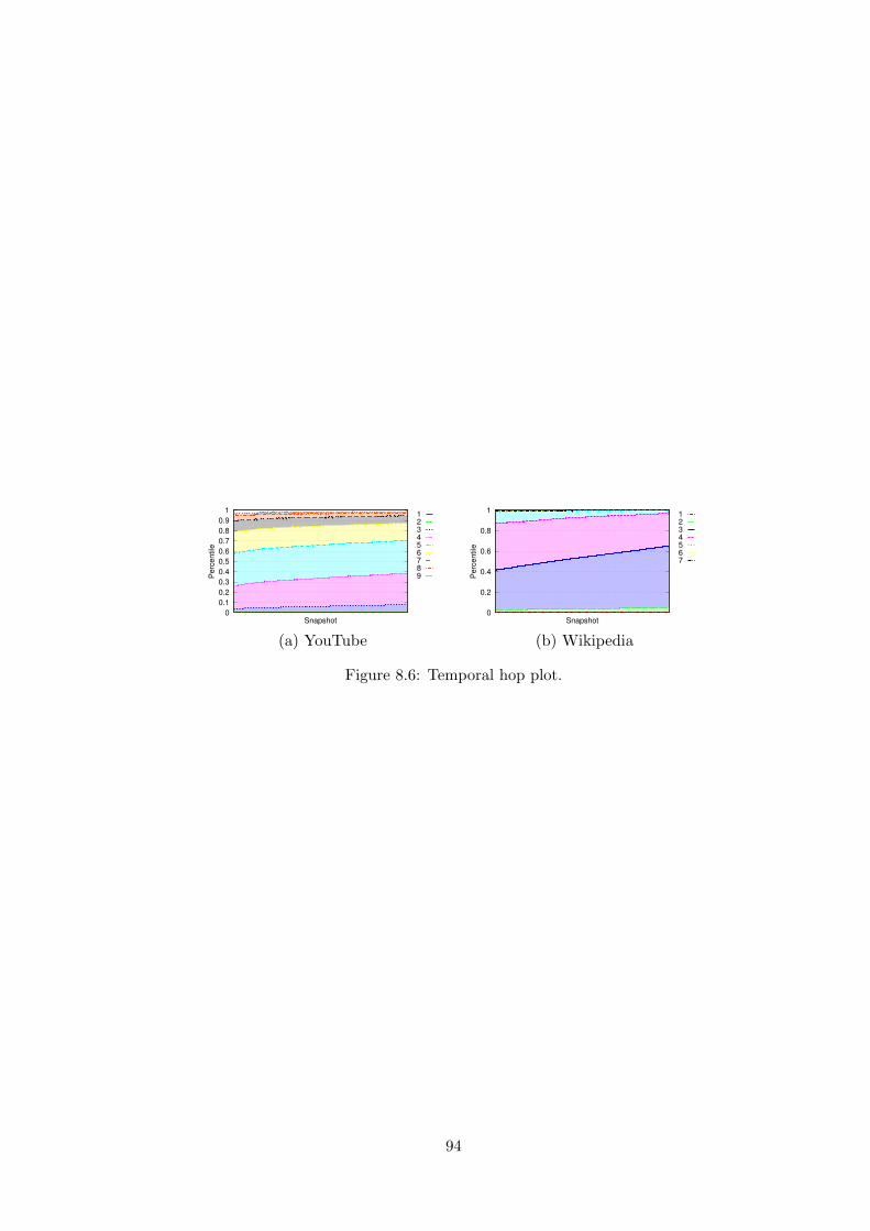
0

0.1

0.2

0.3

0.4

0.5

0.6

0.7

0.8

0.9

1

Pe

rce

ntile

Snapshot

123456789

(a) YouTube

0

0.2

0.4

0.6

0.8

1

Pe

rce

ntile

Snapshot

1234567

(b) Wikipedia

Figure 8.6: Temporal hop plot.

94

Chapter 9

Top-k Distance Queries on Complex

Networks

In this chapter, we study top-k shortest-path distance queries. While manyefficient methods for answering standard (top-1) distance queries have been de-veloped, none of these methods are directly extensible to top-k distance queries.We develop a new framework for top-k distance queries based on 2-hop coverand then present an efficient indexing algorithm based on our pruned landmarklabeling scheme.

First we propse the indexing method for distance queries in Section 9.1, andthen we present the experimental results in Section 9.2. Moreover, in Section 9.3,we discuss the usefulness of top-k distance queries in real applications.

Motivation

As discussed before, the shortest-path distance is widely applied as a proximitymeasure between vertex pairs. However, on complex unweighted graphs suchas social and web graphs, there is a fundamental drawback of basing relevanceon distance alone. Specifically, distances should be integers and the diametersof real-world networks are typically small [Mil67,TM69,WS98,BBR+12,BV12].Such small diameter greatly reduce the number of possible distances and precludethe full use of the underlying structure.

This problem is clearly depicted in Figure 9.1. In each graph in the figure,the distance between the pair of black vertices is four. Hence, based on distancealone, the black pairs in all three graphs have the same similarity. However,the pair in graph (c) seems more tightly connected than the pairs in graphs (a)and (b), since this pair is connected by a greater number of shortest paths.

(a) (b) (c)

Figure 9.1: Examples of connection between two vertices.

95

This intuitive concept can be naturally implemented by adopting the top-kdistances. Table 9.1 presents the top-k distances between the pair of black verticesin each graph of Figure 9.1. Although the pairs in each graph are separated bythe same distance, their top-k distances markedly vary, providing a potentialmeans of distinguishing these three graph structures.

Table 9.1: Distances and top-k distances between the two black vertices in theexamples above.

Graph Distance Top-k Distances

(a) 4 [4, 6, 6, 6, 6, 8, 8, . . . ](b) 4 [4, 4, 4, 6, 6, 6, 6, . . . ](c) 4 [4, 4, 4, 4, 4, 4, 4, . . . ]

Formal Problem Definition

Let P be a set of paths. The i-th shortest path in P refers to the i-th path in P ,ordered by length, where ties are broken arbitrarily. For a pair of vertices (s, t),let Pst be the set of all (unnecessarily simple) paths between s and t. Then fortwo vertices s and t, the i-th shortest path between s and t is the i-th shortestpath in Pst. Let di-th(s, t) denote the length of the i-th shortest path in Pst. Ifthe size of the corresponding set is less than i, then we set them to ∞. We studythe following top-k distance query problem.

Problem 9.1 (Top-k Distance Query).Given: A pair of vertices (s, t).Answer: An array (d1st(s, t), d2nd(s, t), . . . , dk-th(s, t)).

An internal vertex of a path refers to a vertex in the path that is not anendpoint of it. For a vertex v, let P>v

st be the set of paths in Pst whose internal

vertices are all larger than v. Similarly, let P 6>vst be the set of paths in Pst such

that at least one internal vertex is smaller than or equal to v. Let d>vi-th(s, t) and

d 6>vi-th(s, t) denote the length of the i-th shortest path in P>v

st and P 6>vst , respectively.

We define d≥vi-th(s, t) and d 6≥v

i-th(s, t) similarly.

9.1 Top-k Pruned Landmark Labeling

This section describes our proposed method and show its correctness. We alsosuggest several important techniques for practical performance enhancement.

9.1.1 Index Data Structure

The data structure and query algorithm of the proposed method are based on thegeneral framework of 2-hop cover, which is designed for standard (top-1) distancequeries. However, as normal distance queries do not consider the number of paths,the main challenge in processing top-k distance queries is preventing multiplecounts of the same path. To this end, we require a more involved framework.

For each vertex v, our method precomputes and stores the following twolabels:

• Distance label L(v), comprising a set of pairs (u, δ) of a vertex and a pathlength. If we gather lengths in L(v) associated with a vertex u, they shouldform the sequence (d>v

1st(v, u), d>v2nd(v, u), . . . , d

>v`-th(v, u)) for some 1 ≤ ` ≤ k.

96

• Loop label C(v), constituting a sequence of k integers (δ1, δ2, . . . , δk). Thissequence should equal (d≥v

1st(v, v), d≥v2nd(v, v), . . . , d

≥vk-th(v, v)).

An index is a pair I = (L,C), where L and C are the sets of distance labelsL(v)v∈V and loop labels C(v)v∈V , respectively.

9.1.2 Query Algorithm

Given an index I = (L,C) and a pair of vertices (s, t), we compute the top-kdistances between s and t as follows. First, we compute the following multiset.

∆(I, s, t) = δsv + δvv + δvt | (v, δsv) ∈ L(s),

δvv ∈ C(v), (v, δvt) ∈ L(t).

Intuitively, we first move from s to v, then loop back to v several steps later, andfinally move from v to t. Note that from the definition of distance labels andloop labels, every internal vertex in the path from s to t (except v itself) is largerthan v.

Let Query(I, s, t) denote the smallest k elements in the multiset ∆(I, s, t).If |δ(I, s, t)| < k, the remaining entries are filled with ∞. This case occurs onlywhen s and t are disconnected or when s = t and isolated from other vertices.Our answer to the query (s, t) is Query(I, s, t).

9.1.3 Indexing Algorithm

Our index constructing algorithm is summarized in Algorithm 9.1. We first com-pute the loop label C(v) for every vertex v. We then construct the distance labelsL by conducting a pruned BFS from each vertex.

Algorithm 9.1 Indexing Algorithm

1: procedure ConstructIndex(G)2: for i = 1 to n do Compute C(vi) using the modified BFS.3: L(v)← ∅ for all v ∈ V .4: for i = 1 to n do PrunedBFS(G, vi).5: return (C,L).

Algorithm for Computing Loop Labels

We construct the loop labels as follows. For each vertex v, using vertices largerthan or equal to v, we perform a modified version of breadth first search (BFS).In the BFS, each vertex may be visited up to k times. The first k visits to thevertex v gives the distance sequence d≥v

1st(v, v), d≥v2nd(v, v), . . . , d

≥vk-th(v, v).

The modified BFS returns to the starting vertex long before all vertices in thegraph have been visited. Consequently, the running time is very small in practiceand empirically estimated as O(nk) time in total from our experiments.

Algorithm for Computing Distance Labels

We assume that vertices in V are ordered as v1, v2, . . . , vn. Then for each 1 ≤i ≤ n, we perform a pruned BFS from vi (Algorithm 9.2). The pruned BFS isessentially a modified version of the BFS from v that visits the same vertex atmost k times. The crucial difference is the non-trivial pruning; that is, whenvisiting a vertex u at distance δ, the process is discontinued if δ is larger than

97

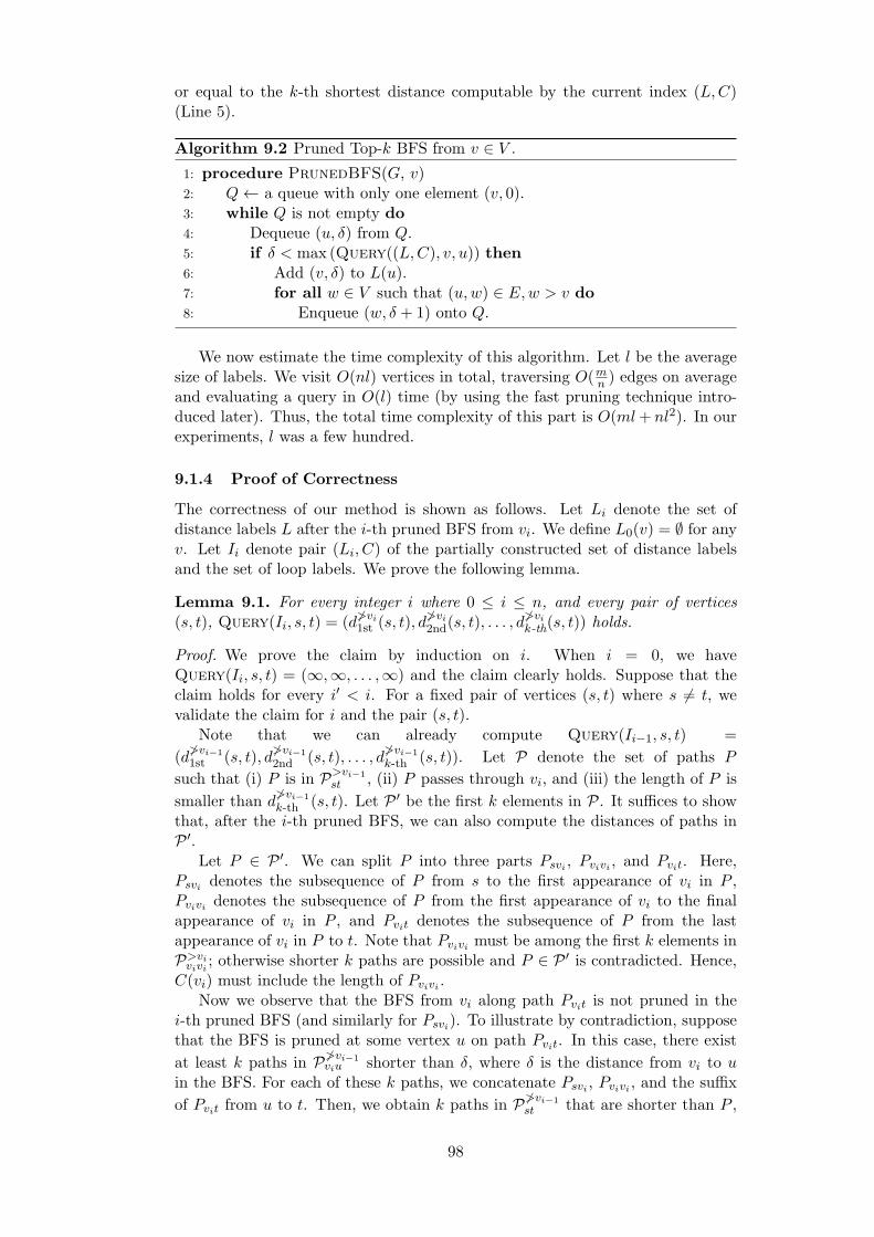
or equal to the k-th shortest distance computable by the current index (L,C)(Line 5).

Algorithm 9.2 Pruned Top-k BFS from v ∈ V .

1: procedure PrunedBFS(G, v)2: Q← a queue with only one element (v, 0).3: while Q is not empty do4: Dequeue (u, δ) from Q.5: if δ < max (Query((L,C), v, u)) then6: Add (v, δ) to L(u).7: for all w ∈ V such that (u,w) ∈ E,w > v do8: Enqueue (w, δ + 1) onto Q.

We now estimate the time complexity of this algorithm. Let l be the averagesize of labels. We visit O(nl) vertices in total, traversing O(mn ) edges on averageand evaluating a query in O(l) time (by using the fast pruning technique intro-duced later). Thus, the total time complexity of this part is O(ml+ nl2). In ourexperiments, l was a few hundred.

9.1.4 Proof of Correctness

The correctness of our method is shown as follows. Let Li denote the set ofdistance labels L after the i-th pruned BFS from vi. We define L0(v) = ∅ for anyv. Let Ii denote pair (Li, C) of the partially constructed set of distance labelsand the set of loop labels. We prove the following lemma.

Lemma 9.1. For every integer i where 0 ≤ i ≤ n, and every pair of vertices(s, t), Query(Ii, s, t) = (d 6>vi

1st (s, t), d6>vi2nd(s, t), . . . , d

6>vik-th(s, t)) holds.

Proof. We prove the claim by induction on i. When i = 0, we haveQuery(Ii, s, t) = (∞,∞, . . . ,∞) and the claim clearly holds. Suppose that theclaim holds for every i′ < i. For a fixed pair of vertices (s, t) where s 6= t, wevalidate the claim for i and the pair (s, t).

Note that we can already compute Query(Ii−1, s, t) =

(d6>vi−1

1st (s, t), d6>vi−1

2nd (s, t), . . . , d6>vi−1

k-th (s, t)). Let P denote the set of paths P

such that (i) P is in P>vi−1

st , (ii) P passes through vi, and (iii) the length of P is

smaller than d6>vi−1

k-th (s, t). Let P ′ be the first k elements in P. It suffices to showthat, after the i-th pruned BFS, we can also compute the distances of paths inP ′.

Let P ∈ P ′. We can split P into three parts Psvi , Pvivi , and Pvit. Here,Psvi denotes the subsequence of P from s to the first appearance of vi in P ,Pvivi denotes the subsequence of P from the first appearance of vi to the finalappearance of vi in P , and Pvit denotes the subsequence of P from the lastappearance of vi in P to t. Note that Pvivi must be among the first k elements inP>vivivi ; otherwise shorter k paths are possible and P ∈ P ′ is contradicted. Hence,

C(vi) must include the length of Pvivi .Now we observe that the BFS from vi along path Pvit is not pruned in the

i-th pruned BFS (and similarly for Psvi). To illustrate by contradiction, supposethat the BFS is pruned at some vertex u on path Pvit. In this case, there exist

at least k paths in P 6>vi−1viu shorter than δ, where δ is the distance from vi to u

in the BFS. For each of these k paths, we concatenate Psvi , Pvivi , and the suffix

of Pvit from u to t. Then, we obtain k paths in P 6>vi−1

st that are shorter than P ,

98

and therefore shorter than d6>vi−1

k-th (s, t) from condition (iii). Hence, we reach acontradiction.

Corollary 9.1. At the end of Algorithm 4.2, we can correctly answer top-k dis-tance queries using the constructed index.

9.1.5 Techniques for Efficient Implementation

We introduce several key techniques for practical performance improvement.

Vertex Ordering Strategy

By properly selecting the order of vertices from which we conduct pruned BFSs,our pruning can drastically reduce the search space and label sizes by exploit-ing the structure of real-world networks, greatly enhancing the efficiency of theproposed method. This is possible because the real networks contain highly cen-tralized vertices (sometimes called hubs). As a heuristic vertex ordering strategy,vertices are selected in order of decreasing degrees. Further discussion is providedin [AIY13].

Fast Pruning

When constructing distance labels, many queries are evaluated for pruning. How-ever, when conducting a pruned BFS from a vertex v, queries are limited to “Arethere more than k paths of length less than δ between v and u?” Given thisrestriction, we can reduce the query time. For each vertex w in the distance labelof v, we can precompute the number cw,δ′ of paths between v and w of length notexceeding δ′ using the loop label C(w). Suppose that we have reached vertex uin the pruned BFS conducted from v. We can then compute the number of pathsbetween v and u of length less than δ as

∑(w,δ′,c)∈L(u) c · cw,δ−δ′ .

Merged Queue Entries

When a (pruned) BFS is performed from a vertex v, rather than pair (u, δ), whichdenotes the existence of a path of length δ between v and u, triplets (u, δ, c) arepushed onto the queue. These triples specify that c paths of length δ exist betweenv and u, This technique enables the simultaneous handling of many paths, andsignificantly reduces the number of pushes onto the queue. Hence, it significantlyreduces the running time.

Merged Label Entries

Related to the above technique, instead of pairs (u, δ), which denotes that thereis a path of length δ between v and u, triplets (u, δ, c) are stored in distancelabels. These triplets indicate that c paths of length δ exist between v and u. Asimilar technique is applicable to loop labels.

9.1.6 Extensions

Directed graphs

If the input graph is a directed graph, we compute and store two distance labelsLIN(v) and LOUT(v) for each vertex v, where LIN(v) and LOUT(v) contain thedistances from and to v, respectively.

99

Weighted graphs

For weighted graphs, we can replace the pruned BFS by pruned Dijkstra’s algo-rithm. In this scheme, the queue used in Algorithm 4.1 is replaced by a priorityqueue. The time complexity becomes O(ml + nl(log n+ l)).

9.2 Experiments

In this section, we show the scalability, efficiency and robustness of the proposedmethod by experimental results using real-world networks.

9.2.1 Setup

Environment

All experiments were conducted on a Linux server with Intel Xeon X5670 (2.93GHz) and 48 GB of main memory. The proposed method was implemented inC++.

Datasets

The target applications of the proposed method are graph mining tasks such asnetwork-aware searching and link prediction. Therefore, our experiments wereconducted on publicly available real-world social and web graphs12345. The sizesand types of these graphs are listed in Table 9.2. We treated all the graphs asunweighted undirected graphs.

Algorithms

As there are no previous indexing methods for top-k distances, the proposedmethod was evaluated against the following two algorithms without precompu-tation.

• The first is the BFS-based naive approach, which uses a FIFO queue inthe graph search, but which allows at most k visits to each vertex. Thisalgorithm was also implemented in C++ by the authors.

• The second is Eppstein’s algorithm [Epp98], which theoretically attainsnear-optimal time complexity. We adopted the C++ implementation ofJon Graehl6.

In what follows, we denote the proposed method by Top-k PLL and these twoprevious methods by BFS and Eppstein.

1http://lovro.lpt.fri.uni-lj.si/support.jsp2http://grouplens.org/datasets/hetrec-2011/3http://snap.stanford.edu/4http://socialnetworks.mpi-sws.org/datasets.html5http://law.di.unimi.it/datasets.php [BV04]6http://www.ics.uci.edu/ eppstein/pubs/p-kpath.html

100

Tab

le9.2:

Dataset

inform

ationan

dperform

ance

oftheproposedandexistingmethodsonreal-worlddatasets

(k=

8).

Dataset

Top-k

PLL

(This

work)

BFS

Eppstein

Nam

eType

|V|

|E|

Indexingtime

Index

size

Querytime

Faceb

ook

-1Social

334

2,218

13.7

ms

178.6

KB

1.9

µs

227.1

µs

378.4

µs

Last.fm

Social

1,89

212,717

125.3

ms

1.3

MB

1.7

µs

1.6

ms

7.5ms

GrQ

cSocial

5,24

214,496

152.9

ms

2.7

MB

1.6

µs

2.2

ms

7.3ms

HepTh

Social

9,87

725,998

631.2

ms

7.8

MB

2.2

µs

5.5

ms

16.5

ms

Con

dMat

Social

23,133

186,936

3.2

s26.4

MB

3.1

µs

15.2

ms

158.8

ms

Faceb

ook

-2Social

63,732

1,545,686

239.0

s716.8

MB

15.2

µs

117.6

ms

2.7s

You

Tube-1

Social

1,15

7,82

84,945,382

624.3

s2.3

GB

5.1

µs

1.5

s7.0s

You

Tube-2

Social

3,23

8,84

818,512,606

1627.1

s9.6

GB

3.9

µs

5.0

s41.1

s

NotreDam

eWeb

325,72

91,497,134

52.3

s617.7

MB

2.9

µs

249.8

ms

1.7s

Stanford

Web

281,90

32,312,497

42.5

s230.0

MB

1.7

µs

454.9

ms

2.9s

BerkStan

Web

685,23

07,600,595

108.7

s1.0

GB

1.9

µs

643.3

ms

10.8

sIndo

Web

1,38

2,90

616,539,644

2695.3

s6.0

GB

12.1

µs

1.4

s25.4

s

101

9.2.2 Indexing Time and Index Size

The high scalability of the proposed method is evident from the index construc-tion time and constructed index size reported in Table 9.2. Indices were con-structed from large social and web graphs comprising tens of millions of edges(YouTube-2 and Indo) in one hour. The index sizes are below 10 GB, easilyaccommodated by the main memories of modern commodity computers.

While the index construction of all datasets was consistently efficient, we ob-serve that the indexing time does not depend on graph size alone. The efficiencyof the proposed method relies on the efficiency of pruning, and is thus related tonetwork properties such as degree distribution and clustering coefficient. How-ever, because the graphs of real-world social, web, computer and biological net-works exhibit similar qualitative properties, the proposed method is robust andconsistently efficient. The same argument is valid for index size.

Figure 9.2a and 9.2b illustrate the effect of k on the indexing time and indexsize in the proposed method. Both are relatively insensitive to the value of k.

10-3

10-2

10-1

100

101

102

103

1 2 4 8 16 32 64

Indexin

g tim

e (

sec)

K

Facebook-1Last.fm

CondMat

(a) Indexing time

10-1

100

101

102

103

1 2 4 8 16 32 64

Index s

ize (

MB

)

K

Facebook-1Last.fm

CondMat

(b) Index size

Figure 9.2: Effect of k on indexing time and index size.

9.2.3 Query Time

The proposed method generally answers queries within microseconds, very muchfaster than the other algorithms (Table 9.2). Indeed for the largest dataset,YouTube-2, the query time was six orders of magnitude faster than those of theBFS-based and Eppstein algorithms. This query time enables top-k distances tobe used in real-time interactive applications such as network-aware search for thefirst time. In our experiments the BFS-based method was faster than Eppstein’salgorithm. This is due to the big constant factor hidden in the O-notation of thetime complexity of Eppstein’s algorithm, as it involves complex data structuremanipulation.

Figure 9.3 plots the query time as a function of k. Although the query timeincreased with k, it remained sufficiently fast at high k.

9.3 Application to Graph Data Mining

In [AHN+15], the usefulness of our indexing method for top-k distance queriesare demonstrated by applying it to the link prediction problem [LNK03]. Inparticular, we confirm that top-k distances can contribute to prediction precisionimprovement. Note that our indexing method enables the first use of the top-kdistances for such tasks, because top-k distances must be computed for manypairs of vertices during training and evaluation.

102

100

101

1 2 4 8 16 32 64

Query

tim

e (

µs)

K

Facebook-1Last.fm

CondMat

Figure 9.3: Effect of k on query time.

We selected link prediction as it is one of the most fundamental and popularproblems on graphs in the AI and Web communities. However, the results suggestthe applicability of top-k distances to other graph tasks such as network-awaresearching.

it is empirically shown that the support vector machine (SVM) with the top-k distances as its feature outperforms a number of baseline methods includingsingular value decomposition and random walk with restart. We emphasize thatour indexing method makes it possible for the first time to use the top-k distancesfor such tasks.

103

Chapter 10

Treewidth and Empirical Graph Tractability

In this chapter, we tackle the long-standing question in this field: what is the keyfactor in addition to network size that has a large effect on the size of constructedindices for graph path queries? As we have discussed several times in this thesis,state-of-the-art graph indexing algorithms, including ours, exploit many commonstructural properties of real-world graphs. Therefore, the performance (i.e., in-dexing time, index size and query time) of such algorithms depends not only thesizes of networks, and indeed vary largely even between networks with almost thesame size (we confirm this point in Section 10.2.1).

Therefore, our goal here is to empirically estimate the tractability (or diffi-culty) of networks. To that end, we propose to use upper bound of treewidthobtained by heuristic tree decomposition algorithms. Here we focus on 2-hop-based indexing methods for distance queries, but we believe that similar resultsalso hold for other problems where state-of-the-art methods are designed to ex-ploit the structures of real networks.

First, as previous decomposition algorithms suffer from the drawback of scal-ability, we present a faster algorithm based on the new notion of star-basedrepresentation in Section 10.1. Then, we discuss the experimental results inSection 10.2. In particular, we confirm that the width of a tree decompositionobtained by our algorithm is indeed informative.

10.1 Tree Decomposition Algorithm

In this section, we give a detailed description of our algorithm for constructing atree decomposition. A naive algorithm for the decomposition can be obtained byextending the well-known min-degree heuristic [BHS03]; however, its scalabilityis highly limited because of its costly clique materialization. To construct the de-compositions for large networks, we propose a new algorithm with several ordersof magnitude better scalability using the new idea of a star-based representation.Our method is also based on the min-degree heuristic; thus we first explain thisheuristic (Section 10.1.1), and then present our new algorithm (Section 10.1.2).

10.1.1 Min-degree Heuristic Algorithm

Our algorithm is based on the min-degree heuristic [BHS03], which is a standardtree decomposition algorithm in practice [XJB05,Wei10,ASK12].

At a high level, the algorithm first generates a list of bags, and then constructsa tree of these bags (Algorithm 10.1). To generate a list of bags, the algorithmrepeatedly reduces a vertex with the smallest degree. The reduction of vertexv includes of three steps. First, we create a new bag Vv including v and all itsneighbors. Second, we change the graph G by removing node v. Third, we create

104

a clique among those vertices in Vv \ v. Then, we construct the tree of thetree decomposition from the list of bags. We set the parent of bag Vv as bag Vp,where (Vv \ v) ⊆ Vp. We can always find the valid parent because all neighborsof a reduced vertex are contained in a clique. Figure 10.1 illustrates a runningexample of the min-degree heuristic algorithm.

Algorithm 10.1 Min-degree heuristic.

1: Repeatedly reduce a vertex with minimum degree to generate a list of bags.2: Add a bag with all the remaining vertices to the list as the root bag.3: Construct a tree of these bags.

Drawback of Scalability Even if we assume that the adjacency lists are man-aged in hash tables and operations on edges can be performed in O(1) time,reducing vertex v takes Θ(|Vv|2) time. Thus, in total, the algorithm takesΘ(

∑t∈T\r |Vt|2) time. Furthermore, we need to materialize edges of cliques;

hence space consumption is also too large. Therefore, even if we use a relativelysmall parameter d (e.g., 100), it becomes impractical to apply the described al-gorithm to large-scale networks.

10.1.2 Proposed Tree Decomposition Algorithm

Overview

The idea behind our method is to virtually conduct the min-degree heuristicalgorithm to avoid costly clique materialization. Rather than naively insertingall the edges of the cliques, we introduce star-based representation to maintainclique edges efficiently. In this representation, all operations on graphs used inthe min-degree heuristic correspond to simple operations, such as modification ofroles of vertices and contraction of edges, which leads to improved scalability ofseveral orders of magnitude.

Star-based Representation Here we deal with two kinds of graphs: A (star-based) representation graph is what we store and maintain in the memory, and arepresented graph corresponds to a virtual snapshot of a graph represented by arepresentation graph that would be maintained by the naive min-degree heuristicalgorithm.

In the star-based representation, each vertex belongs to one of the followingtwo types: normal vertices or hub vertices. Two hub vertices are never connected,i.e., edges connect either two normal vertices or a normal vertex and a hub vertex.The represented graph can be obtained by a representation graph by (1) addingedges to make its neighbors a clique for all hub vertices and (2) removing hubvertices. For example, the representation graphs shown in Figures 10.2a and10.2c represents the graphs shown in Figures 10.2b and 10.2d, respectively.

Overall Algorithm At a high level, our algorithm conducts the min-degreeheuristic (Algorithm 10.1) on virtually represented graphs, i.e., it repeatedlyreduces vertices in the represented graph to generate a list of bags. Then ouralgorithm constructs the tree of the bags. To construct the tree, we use the sametree construction algorithm. Therefore, as noted before, the main difference hereis that, during the reduction phase, we do not maintain the represented graph

105

0

2

4

3

6

5

7

1

89

(a) Theoriginalgraph.

0

2

4

3

6

5

7

1

89

(b) Chosevertex 0.

0

24

1

2

3

4

6

5

7

89

(c) Reduced ver-tex 0.

0

24

1

2

3

4

6

5

7

89

(d) Chose vertex1.

0

2 4

1

2

3

4

2

3

4

6

5

7

8 9

(e) Reduced vertex 1.

0

24

1

2

3

4

2

3

4

6

3

4

5

6

7

8 9

(f) Reduced vertex 2.

0

24

1

2

3

4

2

3

4

6

5

6

7

8

3

4

5

6

7

9

(g) Reduced vertex 8.

0

24

1

2

3

4

2

3

4

6

5

6

7

8

5

6

7

9

3

4

5

6

7

(h) Reduced vertex 9.

Figure 10.1: An example of computation process of a tree decomposition.

itself. We manage the star-based representation graph instead. Thus, we explainhow to reduce vertices using star-based representation for enumerating bags.

Reducing a Vertex First, for an easier case, we consider a situation in whichwe reduce vertex v, whose neighbors are all normal vertices. To remove v andmake its neighbors a clique in the represented graph, we must alter the vertextype of v from normal to hub.

Let us now consider a general situation, where some of v’s neighbors in therepresentation graph are hub vertices. One of the challenges here is the fact

106

6

9

81

7

23

5

4

(a) A star-based representation ofa graph.

6

9

81

7

5

4

(b) The represented graph.

6 9

7

8

1

5

4

(c) The star-based representation af-ter reducing vertex 1.

6 9

7

8

5

4

(d) The represented graph after re-ducing vertex 1.

Figure 10.2: Star-based representation and reduction. The white vertices arenormal vertices, and gray vertices are hub vertices.

that no direct edges can exist in the representation graph between some of v’sneighbors due to these neighbor hub vertices. To make v’s neighbors a clique inthe represented graph, we must create a new hub vertex that is connected to allthese neighbors.

Rather than creating such a new hub from scratch, the new hub can be ef-ficiently composed by contracting v and all the neighboring hub vertices. Con-traction of two vertices means removing the edge between them and merging twoendpoints. For example, reducing the vertex 1 in the represented graph shown inFigure 10.2b corresponds to contracting vertices 1, 2, and 3 in the representationgraph depicted in Figure 10.2a, thus yielding the representation graph in Fig-ure 10.2c. By doing so, as we will discuss in Section 10.1.2, the time complexitybecomes almost linear to the output size using proper data structures. Moreover,we never add any new edge to the representation graph. Therefore, the numberof edges in the representation graph never increases; thus, space consumption isalso kept in linear.

Details

Finding a Vertex to Reduce Precisely finding a vertex with minimum degreeis too costly because we must track the degree of all vertices. Therefore, weapproximately find a vertex with minimum degree by using a priority queue asfollows. First, we insert all vertices into the priority queue, and use their currentdegree as keys. To find a vertex to reduce, we pop a vertex with the smallestkey from the priority queue. If its current degree is the same as the key, then wereduce the vertex. Otherwise, we reinsert the vertex to the priority queue withits new degree.

107

Data Structures We manage adjacency lists in hash tables to operate edgesin constant time. To efficiently contract edges, we manage groups of vertices andmerge adjacency lists, similar to the weighted quick-find algorithm [Yao76].

Time Complexity We roughly estimate the time complexity. As we contractvertices similar to the weighted quick-find algorithm, the expected total timeconsumed for edge contractions is O(m) time [KS78]. Reducing a vertex v takesapproximately O(d′), where d′ is the degree of v. Therefore, we expect that theproposed algorithm computes a tree decomposition in O(

∑i<d idi + m) time,

where di is the number of vertices of degree i.

10.2 Results and Discussion

In Table 10.1, the information of small datasets and results of our tree decompo-sition are given. Note that our tree decompositions are not necessarily optimal,and hence the width given in Table 10.1 is just an upper bound of treewidth.However, the aim of this section is to show how informative the width of a treedecomposition obtained by our algorithm is.

In the following section, we focus on two state-of-the-art indexing methods:pruned landmark labeling and IS-label [FWCW13]. Both are based on the 2-hop cover framework. While both pruned landmark labeling and IS-label usefurther sophisticated frameworks based on 2-hop cover, they can be used to con-struct standard 2-hop indices. Therefore, for simplicity, in our experiments weconstructed standard 2-hop indices by these methods, i.e., pruned landmark la-beling was not combined with the bit-parallel labeling technique and IS-labelconstructed complete vertex hierarchy.

108

Tab

le10.1:Inform

ationof

smalldatasets,

resultsof

ourfulltree

decomposition,andsizesof2-hopindices

constructed

bystate-of-the-artindexing

methodsforshortest-pathdistance

queries.

DatasetInform

ation

Treedecomposition

Distance

Indices

(MB)

Name

|V|

|E|

Type

Tim

e(s)

Width

dd/|V

|PLL

ISL[FW

CW

13]

ca-grqc

5,242

28,980

social(u)

0.02

253

0.048

1.4

3.9

ca-hepth

9,877

51,971

social(u)

0.16

798

0.081

4.4

24.7

wiki-vote

7,115

103,689

social(d)

0.59

1,332

0.187

2.4

23.8

ca-condmat

23,133

186,936

social(u)

1.5

2,160

0.093

13.4

156.8

ca-hepph

12,008

237,010

social(u)

0.52

1,406

0.117

8.8

65.5

email-enron

36,692

367,662

social(d)

1.43

2,178

0.059

8.4

136.1

ca-astroph

18,772

396,160

social(u)

3.34

3,497

0.186

19.5

233.5

email-euall

265,214

420,045

social(d)

1.67

1,033

0.004

84.1

453.0

soc-epinions1

75,879

508,837

social(d)

11.43

5,504

0.073

45.5

1,033.3

soc-slashdot0811

77,360

905,468

social(d)

28.31

8,555

0.111

77.1

1,772.3

soc-slashdot0902

82,168

948,464

social(d)

29.41

9,181

0.112

85.3

2,028.5

web-notredame

325,729

1,497,134

web

(d)

0.99

2,938

0.009

95.4

2,835.4

web-stanford

281,903

2,312,497

web

(d)

2.82

1,611

0.006

64.3

2,086.7

web-google

875,713

5,105,039

web

(d)

80.28

18,229

0.021

712.3

64,540.1

web-berkstan

685,230

7,600,595

web

(d)

10.81

3,272

0.005

195.5

10,482.0

p2p-gnutella08

6,301

20,777

p2p(u)

0.12

1,263

0.200

5.0

26.3

p2p-gnutella09

8,114

26,013

p2p(u)

0.19

1,618

0.199

8.0

43.5

p2p-gnutella06

8,717

31,525

p2p(u)

0.66

2,199

0.252

10.2

65.2

p2p-gnutella05

8,846

31,839

p2p(u)

0.35

2,215

0.250

10.5

65.5

p2p-gnutella04

10,876

39,994

p2p(u)

0.61

2,789

0.256

15.8

102.6

p2p-gnutella25

22,687

54,705

p2p(u)

0.9

3,618

0.159

45.8

284.1

p2p-gnutella24

26,518

65,369

p2p(u)

1.59

4,320

0.163

50.0

389.6

p2p-gnutella30

36,682

88,328

p2p(u)

2.04

5,596

0.153

100.9

707.6

p2p-gnutella31

62,586

147,892

p2p(u)

5.78

9,385

0.150

233.6

2,050.2

cit-hepth

27,770

352,807

citation(d)

11.61

8,515

0.307

158.4

687.0

cit-hepph

34,546

421,578

citation(d)

10.21

10,718

0.310

178.4

1,155.1

109

10.2.1 Non-Trivial Factors for Index Size

We first confirm the existence of non-trivial factors for the index size. Table 10.1lists the sizes of 2-hop indices constructed by the two methods, pruned landmarklabeling and IS-label [FWCW13] for our datasets. The results indicate that,even if two graphs are of similar size, indices constructed from these graphs bythe same algorithm may be of quite different sizes.

For example, datasets email-enron, ca-astroph, cit-hepth and cit-hepph

have similar sizes in terms of the number of vertices and edges. However, sizesof indices for these datasets vary largely and, surprisingly, indices for cit-hepphare approximately ten times larger than those for email-enron for both indexingalgorithms. Similar differences can be observed from datasets ca-condmat andp2p-gnutella30.

This is because these state-of-the-art indexing methods heuristically exploitthe structures of real networks explicitly or implicitly, and thus they depend onthe properties of each network. Indeed, it is proved that 2-hop indices may haveΘ(n2) space for general graphs [GPPR04]. Therefore, it is impossible to constructsmall 2-hop indices without exploiting the network structures.

However, the long-standing question among researchers in this field is that,having understood this, what is the key factor besides network size that hasa large effect on the size of constructed shortest-path distance indices? In thefollowing section, we show that obtaining the width of a tree decomposition cantake us closer to the answer.

10.2.2 Qualitative Empirical Analysis

Widths of tree decompositions obtained using our algorithm are also listed inTable 10.1. We can observe that the difference in index sizes seems to be highlyrelated to widths. For example, widths of the tree decompositions for datasetsemail-enron and cit-hepph are 10,718 and 2,178, respectively. Similarly, treedecompositions for ca-condmat and p2p-gnutella30 have widths of 1,406 and5,596, respectively.

Interestingly, from our results, index sizes for graphs with larger widths arealmost always larger than those for graphs with smaller widths. Therefore,treewidth could be the key factor that has a large effect on the sizes of con-structed shortest-path distance indices.

10.2.3 Quantitative Empirical Analysis

To further analyze the relation between widths of tree decompositions and sizesof distance indices, let us recall the theoretical results discussed in Section 4.3.4.Theorem 4.4 tells that, while there are no non-trivial theoretical bounds on thesize of 2-hop indices that are better than O(n2) for general graphs [GPPR04],we can prove that there are small 2-hop indices for graphs of small treewidth.Specifically, it says that there is a 2-hop index with size O(nw log n) for a graphwith treewidth w.

Although the aforementioned methods do not necessarily yield 2-hop indicesof that size (i.e., O(nw log n)), we show that this theoretical bound works quitewell as an estimation. Figure 10.3 illustrates the relation between the estimatedvalue nw log n and actual sizes of constructed indices showing that these valuescorrelate well.

Moreover, in Table 10.2, we see that Spearman’s correlation coefficient be-tween estimation nd log n and actual index sizes is significantly higher than other

110

100

101

102

103

104

105

106

107

108

109

1010

1011

1012

Ind

ex s

ize

(M

B)

n d log(n)

PLLISL

Figure 10.3: Actual index sizes and estimation using the widths of tree decom-positions.

estimations such as n and m. This indicates that the width d of our tree decom-position is indeed informative. Note that Spearman’s correlation coefficient usesonly ranks and thus, for example, the score for estimation of n2 would be exactlythe same as that of n.

Table 10.2: Spearman’s correlation between actual index sizes and estimationwith and without width d.

Methods n m n+m d nd log n

PLL 0.819 0.774 0.798 0.795 0.899IS-Label [FWCW13] 0.940 0.792 0.875 0.719 0.983

111

Chapter 11

Conclusions

In this thesis, we studied graph indexing methods for path-related queries. Previ-ously, state-of-the-art methods for different queries or different families of graphsare developed almost independently, and their approaches were also quite dif-ferent. Even limiting to labeling-based methods, their labeling algorithms weretotally different. By contrast, the methods presented in this thesis are based onthe same notion of pruned labeling, which were demonstrated to be competitiveor comparable with state-of-the-art methods for each kind of query. Specifi-cally, we designed indexing methods for reachability queries on directed acycilicgraphs, shortest-path queries on road networks, historical shortest-path querieson evolving networks, and top-k shortest-path queries on complex networks. Wedemonstrated that each of these methods is also comparable with state-of-the-artmethods for each kind of query, thus showing exceptional generality of our unifiedapproach.

Lastly, we discuss the follow-up work of our pruned labeling algorithms byother groups and future work in this field.

Follow-up Work

The emergence of pruned labeling algorithms have had large impact to researchcommunities. As evidence, there have already been several papers presentingfollow-up work of them by other groups. We introduce a few notable results.

More robust vertex ordering strategies [DGPW14] As we observed, onmany network instances with skewed degree distribution, simple vertex orderingstrategies such as the Degree strategy work surprisingly well. However, Dellinget al. show that, by approximately solving optimization problems, better vertexorders can be obtained for pruned labeling, which lead to further smaller labelsizes. Moreover, they also showed that their ordering strategies are much morerobust, in the sense that they can find good vertex ordering on various kinds ofgraph families.

Fully dynamic indexing for reachability queries [ZLWX14] We have pre-sented incremental index update algorithm based on pruned labeling against edgeinsertion. Zhu et al. have also independently proposed index update algorithmbased on pruned labeling for labeling-based reachability indices. In contrast toour discussion, they focus on vertex insertion and vertex removal. Vertex removalis much slower than vertex insertion, though it is faster than full reconstruction.

112

External memory labeling algorithm [JFWX14] Our indexing algorithmassumed that given graphs fit in main memory, and does not work well whenthey are in external memory due to frequent random access. Jiang et al. deviseda labeling algorithm for the 2-hop cover framework, which can efficiently processgraphs in external memory. It is also built on the notion of pruned labeling.

Future Work

More scalability While our methods improved the scalability of exact graphquerying (e.g., distance queries on complex networks) by orders of magnitude,they are still not sufficiently scalable when considering huge social and webgraphs, which may consist of billions of vertices and edges. Therefore, we stillneed more scalable indexing methods.

Complex queries Some of real applications requires path-related queries thathave more involved constraints. For example, in graph database systems, answer-ing path queries with label constraints is a fundamental building block [LB13],which cannot be efficiently processed by our current indexing techniques.

Stronger connection to theory Unfortunately, besides the seminal workmentioned in Chapter 3, theoretical research has had little impact to practicalalgorithms. This is because the interest of the theory community (e.g., worst-case asymptotic complexity on general graphs) is in a quite different directionfrom reality (e.g., real running time on real instances). Such discrepancy is quitecommon in the field of algorithmics. This work sometimes borrowed ideas fromgraph theory and theoretical graph algorithms, such as tree decomposition. Theremight be more theoretical ideas that are actually useful in practice. Contrary tothis, the author also hopes to contribute to the calibration of current theoreticalfields from the practice side.

113

List of Figures

1.1 A social ego network of the author (i.e., the subgraph induced bythe friends of the authors) extracted from Facebook by Netvizz1. . 2

1.2 A part of a road network of the City of New York [DGJ09]. Redand blue paths illustrate the shortest paths between the same pairof vertices, where the red one optimizes distance and the blue oneoptimizes time. . . . . . . . . . . . . . . . . . . . . . . . . . . . . 3

1.3 The necessity of graph indexing methods. . . . . . . . . . . . . . . 51.4 The overview of graph indexing methods. . . . . . . . . . . . . . . 51.5 The performance trade-off of indexing methods between scalability

and query performance. . . . . . . . . . . . . . . . . . . . . . . . . 61.6 A general illustration of incremental index update. . . . . . . . . . 91.7 Organization of this thesis. . . . . . . . . . . . . . . . . . . . . . . 12

2.1 An example of tree decomposition. . . . . . . . . . . . . . . . . . 18

3.1 The index data structure and query algorithm of the 2-hop coverframework. . . . . . . . . . . . . . . . . . . . . . . . . . . . . . . . 23

3.2 The index construction process of tree-decomposition-based ap-proaches. . . . . . . . . . . . . . . . . . . . . . . . . . . . . . . . . 25

3.3 The query algorithm of tree-decomposition-based distance querying. 263.4 The index construction process of contraction hierarchies. Blue,

yellow and red vertices denote those which are not yet contracted,already contracted and just being contracted, respectively. . . . . . 28

4.1 Examples of pruned BFSs. Yellow vertices denote the roots, bluevertices denote those which we visited and labeled, red verticesdenote those which we visited but pruned, and gray vertices denotethose which are already used as roots. . . . . . . . . . . . . . . . . 35

4.2 A running example for the update algorithm. The green vertex isthe root, and the distance to the root is written in each vertex. . 41

5.1 The key insight of the bit-parallel labeling scheme. . . . . . . . . . 465.2 Properties of the static complex network datasets. . . . . . . . . . 505.3 Effect of pruning and sizes of labels. . . . . . . . . . . . . . . . . . 555.4 Fraction of pairs of vertices whose distance can be answered by

index, against number of performed pruned BFS. . . . . . . . . . . 565.5 Performance varing number of bit-parallel BFSs. . . . . . . . . . . 575.6 Update time on synthetic networks with different size and density. 58

6.1 An example of pruned path labeling. Color of a vertex indicatesits status: Red is a start point of BFSs, blue is a vertex beingsearched, gray is a pruned vertex, and brown is a vertex alreadyused as a start point. . . . . . . . . . . . . . . . . . . . . . . . . . . 65

6.2 Performance comparison of reachability queries on synthetic graphs. 72

114

7.1 Examples for the pruned highway labeling. Pink vertices are on thestarting path Pi, blue vertices are visited and added to some labels,gray vertices are already used as the starting points of the previoussearches, orange vertices are visited but pruned, and white verticesare not visited. . . . . . . . . . . . . . . . . . . . . . . . . . . . . . 78

7.2 Effect of pruning. . . . . . . . . . . . . . . . . . . . . . . . . . . . . 827.3 Label properties. . . . . . . . . . . . . . . . . . . . . . . . . . . . . 83

8.1 An illustration of indexing methods for historical queries. . . . . . 848.2 Label size for historical queries on synthetic networks with different

size and density. . . . . . . . . . . . . . . . . . . . . . . . . . . . . 908.3 An example of social network analysis on a dynamic Facebook

subgraph [VMCG09] using our method for historical shortest-pathdistance queries. . . . . . . . . . . . . . . . . . . . . . . . . . . . . 92

8.4 Transition of average distance and effective diameter. . . . . . . . . 938.5 Transition of the closeness centrality of some popular vertices. . . . 938.6 Temporal hop plot. . . . . . . . . . . . . . . . . . . . . . . . . . . . 94

9.1 Examples of connection between two vertices. . . . . . . . . . . . . 959.2 Effect of k on indexing time and index size. . . . . . . . . . . . . . 1029.3 Effect of k on query time. . . . . . . . . . . . . . . . . . . . . . . . 103

10.1 An example of computation process of a tree decomposition. . . . . 10610.2 Star-based representation and reduction. The white vertices are

normal vertices, and gray vertices are hub vertices. . . . . . . . . 10710.3 Actual index sizes and estimation using the widths of tree decom-

positions. . . . . . . . . . . . . . . . . . . . . . . . . . . . . . . . . 111

115

List of Tables

2.1 Notations . . . . . . . . . . . . . . . . . . . . . . . . . . . . . . . . 13

5.1 Static complex network datasets . . . . . . . . . . . . . . . . . . . 495.2 Dynamic Complex Network Datasets . . . . . . . . . . . . . . . . . 515.3 Performance comparison between the proposed method and pre-

vious methods for the real-world datasets. IT denotes indexingtime, IS denotes index size, QT denotes query time, and LN de-notes average label size for each vertex. DNF means it did notfinish in one day or ran out of memory. . . . . . . . . . . . . . . . 53

5.4 Average size of a label for each vertex against different vertexordering strategies. . . . . . . . . . . . . . . . . . . . . . . . . . . . 56

5.5 Performance results without bit-prallel BFSs. . . . . . . . . . . . . 575.6 Experimental results of our online update algorithm. . . . . . . . . 58

6.1 Real-world datasets for reachability queries . . . . . . . . . . . . . 706.2 Average query time (µs) . . . . . . . . . . . . . . . . . . . . . . . . 706.3 Index size (MB) . . . . . . . . . . . . . . . . . . . . . . . . . . . . . 716.4 Indexing time (sec) . . . . . . . . . . . . . . . . . . . . . . . . . . . 716.5 Comparison of index size of PLL using different vertex ordering

strategies (MB) . . . . . . . . . . . . . . . . . . . . . . . . . . . . . 736.6 Comparison of index size of PPL using different path selection

strategies (MB) . . . . . . . . . . . . . . . . . . . . . . . . . . . . . 73

7.1 Comparison of the performance between pruned highway labelingand previous methods. HL is parallelized to use 12 cores in pre-processing and all other methods are not parallelized. . . . . . . . 81

7.2 Comparison of the performance by the contraction technique. Thecontraction level indicates the degree of removed vertices. . . . . . 82

8.1 Experimental results of our method for historical queries againstreal-world and synthetic networks. . . . . . . . . . . . . . . . . . . 91

9.1 Distances and top-k distances between the two black vertices inthe examples above. . . . . . . . . . . . . . . . . . . . . . . . . . . 96

9.2 Dataset information and performance of the proposed and existingmethods on real-world datasets (k = 8). . . . . . . . . . . . . . . . 101

10.1 Information of small datasets, results of our full tree decompo-sition, and sizes of 2-hop indices constructed by state-of-the-artindexing methods for shortest-path distance queries. . . . . . . . . 109

10.2 Spearman’s correlation between actual index sizes and estimationwith and without width d. . . . . . . . . . . . . . . . . . . . . . . . 111

116

References

[ABJ89] R. Agrawal, A. Borgida, and H. V. Jagadish. Efficient manage-ment of transitive relationships in large data and knowledge bases.In SIGMOD, pages 253–262, 1989.

[ADGW11] I. Abraham, D. Delling, A. V. Goldberg, and R. F. Werneck. Ahub-based labeling algorithm for shortest paths in road networks.In SEA, pages 230–241, 2011.

[ADGW12] I. Abraham, D. Delling, A. V. Goldberg, and R. F. Werneck.Hierarchical hub labelings for shortest paths. In ESA, pages 24–35. 2012.

[AFGW10] I. Abraham, A. Fiat, A. V. Goldberg, and R. F. Werneck. High-way dimension, shortest paths, and provably efficient algorithms.In SODA, pages 782–793, 2010.

[AG06] I. Abraham and C. Gavoille. Object location using path separa-tors. In PODC, pages 188–197, 2006.

[AHN+15] T. Akiba, T. Hayashi, N. Nori, Y. Iwata, and Y. Yoshida. Efficienttop-k shortest-path distance queries on large networks by prunedlandmark labeling. In AAAI, 2015. to appear.

[AIKK14] T. Akiba, Y. Iwata, K. Kawarabayashi, and Y. Kawata. Fastshortest-path distance queries on road networks by pruned high-way labeling. In ALENEX, pages 147–154, 2014.

[AIY13] T. Akiba, Y. Iwata, and Y. Yoshida. Fast exact shortest-pathdistance queries on large networks by pruned landmark labeling.In SIGMOD, pages 349–360, 2013.

[AIY14] T. Akiba, Y. Iwata, and Y. Yoshida. Dynamic and histori-cal shortest-path distance queries on large evolving networks bypruned landmark labeling. In WWW, pages 237–248, 2014.

[AJB99] R. Albert, H. Jeong, and A. L. Barabasi. The diameter of theworld wide web. Nature, 401:130–131, 1999.

[ALM09] F. Aidouni, M. Latapy, and C. Magnien. Ten weeks in the life ofan edonkey server. In IPDPS, pages 1–5, 2009.

[AMK14] T. Akiba, T. Maehara, and K. Kawarabayashi. Network struc-tural analysis via core-tree-decomposition. Manuscript, 2014.

[AP89] S. Arnborg and A. Proskurowski. Linear time algorithms for np-hard problems restricted to partial k-trees. Discrete Appl. Math.,2:11–24, 1989.

117

[APPB10] V. Agarwal, F. Petrini, D. Pasetto, and D. A. Bader. Scalablegraph exploration on multicore processors. In SC, pages 1–11,2010.

[ASK12] T. Akiba, C. Sommer, and K. Kawarabayashi. Shortest-pathqueries for complex networks: exploiting low tree-width outsidethe core. In EDBT, pages 144–155, 2012.

[BA99] A.-L. Barabasi and R. Albert. Emergence of scaling in randomnetworks. Science, 286(5439):509–512, 1999.

[Bar05] A.-L. Barabasi. The origin of bursts and heavy tails in humandynamics. Nature, 435:207–211, 2005.

[BBR+12] L. Backstrom, P. Boldi, M. Rosa, J. Ugander, and S. Vigna. Fourdegrees of separation. In WebSci, pages 33–42, 2012.

[BCSV04] P. Boldi, B. Codenotti, M. Santini, and S. Vigna. Ubicrawler:A scalable fully distributed web crawler. Software Pract. Ex.,34(8):711–726, 2004.

[BDG+14] H. Bast, D. Delling, A. Goldberg, M. Muller-Hannemann, T. Pa-jor, P. Sanders, D. Wagner, and R. Werneck. Route planningin transportation networks. Technical report, MSR-TR-2014-4,2014.

[BDS+10] R. Bauer, D. Delling, P. Sanders, D. Schieferdecker, D. Schultes,and D. Wagner. Combining hierarchical and goal-directed speed-up techniques for dijkstra’s algorithm. J. Exp. Algorithmics,15(2.3):1–31, 2010.

[Bel58] R. E. Bellman. On a routing problem. Quarterly of AppliedMathematics, 16:87–90, 1958.

[BFM+07] H. Bast, S. Funke, D. Matijevic, P. Sanders, and D. Schultes. Intransit to constant time shortest-path queries in road networks.In ALENEX, pages 46–59, 2007.

[BGJ+12] A. Bhattacharyya, E. Grigorescu, K. Jung, S. Raskhodnikova,and D. P. Woodruff. Transitive-closure spanners. SIAM J. Com-put., 41(6):1380–1425, 2012.

[BHKL06] L. Backstrom, D. Huttenlocher, J. Kleinberg, and X. Lan. Groupformation in large social networks: membership, growth, and evo-lution. In KDD, pages 44–54, 2006.

[BHS03] A. Berry, P. Heggernes, and G. Simonet. The minimum degreeheuristic and the minimal triangulation process. In WG, volume2880 of LNCS, pages 58–70. 2003.

[BKM+00] A. Broder, R. Kumar, F. Maghoul, P. Raghavan, S. Rajagopalan,R. Stata, A. Tomkins, and J. Wiener. Graph structure in the web.Computer Networks: The International Journal of Computer andTelecommunications Networking, 33(1-6):309–320, June 2000.

[BLM+06] S. Boccaletti, V. Latora, Y. Moreno, M. Chavez, and D. Hwang.Complex networks: Structure and dynamics. Physics reports,424(4-5):175–308, 2006.

118

[BMSV14] P. Boldi, A. Marino, M. Santini, and S. Vigna. Bubing: Massivecrawling for the masses. In WWW Companion, pages 227–228,2014.

[BRSV11] P. Boldi, M. Rosa, M. Santini, and S. Vigna. Layered label propa-gation: a multiresolution coordinate-free ordering for compressingsocial networks. In WWW, pages 587–596, 2011.

[BV04] P. Boldi and S. Vigna. The webgraph framework I: compressiontechniques. In WWW, pages 595–602, 2004.

[BV12] P. Boldi and S. Vigna. Four degrees of separation, really. InASONAM, pages 1222–1227, 2012.

[Car71] B. A. Carre. An algebra for network routing problems. IMA J.Appl. Math., 7(3):273–294, 1971.

[CGK05] L. Chen, A. Gupta, and M. Kurul. Stack-based algorithms forpattern matching on dags. In VLDB, pages 493–504, 2005.

[Cha03] D. Chamberlin. XQuery: a query language for XML. In SIG-MOD, pages 682–682, 2003.

[CHKZ03] E. Cohen, E. Halperin, H. Kaplan, and U. Zwick. Reachabil-ity and distance queries via 2-hop labels. SIAM J. Comput.,32(5):1338–1355, 2003.

[CNSW00] D. S. Callaway, M. E. J. Newman, S. H. Strogatz, and D. J.Watts. Network robustness and fragility: Percolation on randomgraphs. Phys. Rev. Lett., 85:5468–5471, 2000.

[CSTW12] W. Chen, C. Sommer, S.-H. Teng, and Y. Wang. A compactrouting scheme and approximate distance oracle for power-lawgraphs. TALG, 9(1):4:1–26, 2012.

[CY09] J. Cheng and J. X. Yu. On-line exact shortest distance queryprocessing. In EDBT, pages 481–492, 2009.

[CYL+06] J. Cheng, J. X. Yu, X. Lin, H. Wang, and P. S. Yu. Fast compu-tation of reachability labeling for large graphs. In EDBT, pages961–979, 2006.

[DGJ09] C. Demetrescu, A. V. Goldberg, and D. S. Johnson. The ShortestPath Problem: Ninth DIMACS Implementation Challenge, vol-ume 74. AMS, 2009.

[DGPW14] D. Delling, A. V. Goldberg, T. Pajor, and R. F. Werneck. Robustdistance queries on massive networks. In ESA, pages 321–333,2014.

[DGSF14] D. Delling, A. V. Goldberg, R. Savchenko, and R. F.Werneck.Hub labels: Theory and practice. In SEA, pages 259–270, 2014.

[DGW13] D. Delling, A. V. Goldberg, and R. F. Werneck. Hub label com-pression. In SEA, pages 18–29, 2013.

[Dij59] E. W. Dijkstra. A note on two problems in connexion with graphs.Numerische Mathematik, 1(1):269–271, 1959.

119

[DMS00] S. N. Dorogovtsev, J. F. F. Mendes, and A. N. Samukhin. Struc-ture of growing networks with preferential linking. Phys. Rev.Lett., 85:4633–4636, 2000.

[Epp98] D. Eppstein. Finding the k shortest paths. SIAM J. Computing,28(2):652–673, 1998.

[FFF99] M. Faloutsos, P. Faloutsos, and C. Faloutsos. On power-law rela-tionships of the Internet topology. In SIGCOMM, pages 251–262,1999.

[Flo62] R. W. Floyd. Algorithm 97: Shortest path. Comm. ACM,5(6):345, 1962.

[FLWW12] W. Fan, J. Li, X. Wang, and Y. Wu. Query preserving graphcompression. In SIGMOD, pages 157–168, 2012.

[For56] L. R. Ford. Network flow theory. Report P-923, The Rand Cor-poration, 1956.

[FT87] M. L. Fredman and R. E. Tarjan. Fibonacci heaps and theiruses in improved network optimization algorithms. J. ACM,34(3):596–615, 1987.

[FWCW13] A. W.-C. Fu, H. Wu, J. Cheng, and R. C.-W. Wong. Is-label: anindependent-set based labeling scheme for point-to-point distancequerying. PVLDB, 6(6):457–468, 2013.

[GBSW10] A. Gubichev, S. Bedathur, S. Seufert, and G. Weikum. Fast andaccurate estimation of shortest paths in large graphs. In CIKM,pages 499–508, 2010.

[GH05] A. V. Goldberg and C. Harrelson. Computing the shortest path:A* search meets graph theory. In SODA, 2005.

[GPPR04] C. Gavoille, D. Peleg, S. Perennes, and R. Raz. Distance labelingin graphs. J. Algorithms, 53(1):85 – 112, 2004.

[GSSD08] R. Geisberger, P. Sanders, D. Schultes, and D. Delling. Contrac-tion hierarchies: Faster and simpler hierarchical routing in roadnetworks. In WEA, pages 319–333, 2008.

[Gut04] R. Gutman. Reach-based routing: A new approach to shortestpath algorithms optimized for road networks. In ALENEX, 2004.

[Hal76] R. Halin. s-function for graphs. J. Geometry, 8:171–186, 1976.

[HL71] P. W. Holland and S. Leinhardt. Transitivity in structural modelsof small groups. Small Group Research, 2(2):107–124, 1971.

[HWYY07] H. He, H. Wang, J. Yang, and P. S. Yu. Blinks: ranked keywordsearches on graphs. In SIGMOD, pages 305–316, 2007.

[IHI+94] T. Ikeda, M. Y. Hsu, H. Imai, S. Nishimura, H. Shimoura,T. Hashimoto, K. Tenmoku, and K. Mitoh. A fast algorithmfor finding better routes by ai search techniques. In VNSI, pages291–296, 1994.

120

[JFWX14] M. Jiang, A. W. Fu, R. C. Wong, and Y. Xu. Hop doublinglabel indexing for point-to-point distance querying on scale-freenetworks. PVLDB, 7(12):1203–1214, 2014.

[Jor69] C. Jordan. Sur les assemblages de lignes. J. Reine Angew Math,70:185–190, 1869.

[JRDX12] R. Jin, N. Ruan, S. Dey, and J. Xu. SCARAB: scaling reachabilitycomputation on large graphs. In SIGMOD, pages 169–180, 2012.

[JRXL12] R. Jin, N. Ruan, Y. Xiang, and V. Lee. A highway-centric labelingapproach for answering distance queries on large sparse graphs.In SIGMOD, pages 445–456, 2012.

[JXRF09] R. Jin, Y. Xiang, N. Ruan, and D. Fuhry. 3-hop: a high-compression indexing scheme for reachability query. In SIGMOD,pages 813–826, 2009.

[JXRW08] R. Jin, Y. Xiang, N. Ruan, and H. Wang. Efficiently answeringreachability queries on very large directed graphs. In SIGMOD,pages 595–608, 2008.

[Kar29] F. Karinthy. Lancszemek. 1929.

[KKT03] D. Kempe, J. Kleinberg, and E. Tardos. Maximizing the spreadof influence through a social network. In KDD, pages 137–146,2003.

[KMS06] E. Kohler, R. H. Mohring, and H. Schilling. Fast point-to-pointshortest path computations with arc-flags. In The Shortest PathProblem: Ninth DIMACS Implementation Challenge, pages 41–72, 2006.

[KS78] D. E. Knuth and A. Schonhage. The expected linearity of a simpleequivalence algorithm. Theor. Comput. Sci., 6:281–315, 1978.

[Kur30] K. Kuratowski. Sur le Probleme des Courbes Gauches en Topolo-gie. Fundamenta Mathematicae, 15:271–283, 1930.

[KY04] B. Klimt and Y. Yang. The enron corpus: A new dataset foremail classification research. In ECML, volume 3201 of LNCS,pages 217–226. 2004.

[LB13] A. Likhyani and S. Bedathur. Label constrained shortest pathestimation. In CIKM, pages 1177–1180, 2013.

[LG14] F. Le Gall. Powers of tensors and fast matrix multiplication. InISSAC, pages 296–303, 2014.

[LHK10a] J. Leskovec, D. Huttenlocher, and J. Kleinberg. Predicting posi-tive and negative links in online social networks. In WWW, pages641–650, 2010.

[LHK10b] J. Leskovec, D. Huttenlocher, and J. Kleinberg. Signed networksin social media. In CHI, pages 1361–1370, 2010.

121

[LKF05] J. Leskovec, J. Kleinberg, and C. Faloutsos. Graphs over time:Densification laws, shrinking diameters and possible explanations.In KDD, pages 177–187, 2005.

[LKF07] J. Leskovec, J. Kleinberg, and C. Faloutsos. Graph evolution:Densification and shrinking diameters. TKDD, 1(1), 2007.

[LLDM09] J. Leskovec, K. Lang, A. Dasgupta, and M. Mahoney. Communitystructure in large networks: Natural cluster sizes and the absenceof large well-defined clusters. Internet Mathematics, 6(1):29–123,2009.

[LNK03] D. Liben-Nowell and J. Kleinberg. The link prediction problemfor social networks. In CIKM, pages 556–559, 2003.

[MA05] P. Massa and P. Avesani. Controversial users demand local trustmetrics: an experimental study on epinions.com community. InAAAI, pages 121–126, 2005.

[MAIK14] T. Maehara, T. Akiba, Y. Iwata, and K. Kawarabayashi. Com-puting personalized pagerank quickly by exploiting graph struc-tures. PVLDB, 7(12):1023–1034, 2014.

[Mil67] S. Milgram. The small world problem. Psychology Today, 1:61–67,1967.

[Mis09] A. Mislove. Online Social Networks: Measurement, Analysis, andApplications to Distributed Information Systems. PhD thesis,Rice University, 2009.

[MLH09] C. Magnien, M. Latapy, and M. Habib. Fast computation ofempirically tight bounds for the diameter of massive graphs. J.Exp. Algorithmics, 13:10:1.10–10:1.9, February 2009.

[MMG+07] A. Mislove, M. Marcon, K. P. Gummadi, P. Druschel, andB. Bhattacharjee. Measurement and analysis of online social net-works. In IMC, pages 29–42, 2007.

[MVLB14] R. Meusel, S. Vigna, O. Lehmberg, and C. Bizer. Graph structurein the web — revisited: A trick of the heavy tail. In WWWCompanion, pages 427–432, 2014.

[NSW01] M. E. J. Newman, S. H. Strogatz, and D. J. Watts. Randomgraphs with arbitrary degree distributions and their applications.Phys. Rev. E, 64(2):026118 1–17, 2001.

[Nuu95] E. Nuutila. Effcient transitive closure computation in large di-graphs. PhD thesis, Finnish Academy of Technology, 1995.

[PAG09] J. Perez, M. Arenas, and C. Gutierrez. Semantics and complex-ity of SPARQL. Transactions on Database Systems, 34(3):16:1–16:45, September 2009.

[PBCG09] M. Potamias, F. Bonchi, C. Castillo, and A. Gionis. Fast shortestpath distance estimation in large networks. In CIKM, pages 867–876, 2009.

122

[PBMW99] L. Page, S. Brin, R. Motwani, and T. Winograd. The PageRankcitation ranking: Bringing order to the web. Technical report,Stanford InfoLab, 1999.

[PSV04] R. Pastor-Satorras and A. Vespignani. Evolution and structureof the Internet: A statistical physics approach. Cambridge Uni-versity Press, 2004.

[QCCY12] M. Qiao, H. Cheng, L. Chang, and J. X. Yu. Approximateshortest distance computing: A query-dependent local landmarkscheme. In ICDE, pages 462–473, 2012.

[RAD03] M. Richardson, R. Agrawal, and P. Domingos. Trust managementfor the semantic web. In ISWC, volume 2870, pages 351–368.2003.

[RAS+05] S. A. Rahman, P. Advani, R. Schunk, R. Schrader, and D. Schom-burg. Metabolic pathway analysis web service (pathway huntertool at cubic). Bioinformatics, 21(7):1189–1193, 2005.

[Rep97] T. Reps. Program analysis via graph reachability. In ILPS, pages5–19, 1997.

[RHS95] T. Reps, S. Horwitz, and M. Sagiv. Precise interproceduraldataflow analysis via graph reachability. In POPL, pages 49–61,1995.

[RIF02] M. Ripeanu, A. Iamnitchi, and I. Foster. Mapping the gnutellanetwork. IEEE Internet Computing, 6(1):50–57, January 2002.

[RPFM14] M. P. Rombach, M. A. Porter, J. H. Fowler, and P. J. Mucha.Core-Periphery Structure in Networks. SIAM J. Appl. Math.,74(1):167–190, February 2014.

[RS84] N. Robertson and P. D. Seymour. Graph minors. III. planar tree-width. J. Comb. Theory, Ser. B, 36(1):49–64, 1984.

[RS04] N. Robertson and P. Seymour. Graph minors. XX. wagner’s con-jecture. J. Comb. Theory, Ser. B, 92(2):325 – 357, 2004. SpecialIssue Dedicated to Professor W.T. Tutte.

[RS06] S. A. Rahman and D. Schomburg. Observing local and globalproperties of metabolic pathways: ‘load points’ and ‘choke points’in the metabolic networks. Bioinformatics, 22(14):1767–1774,2006.

[Sim88] K. Simon. An improved algorithm for transitive closure on acyclicdigraphs. Theor. Comput. Sci., 58(1):325–346, 1988.

[Som14] C. Sommer. Shortest-path queries in static networks. ACM Com-put. Surv.ag, 46:45:1–31, 2014.

[STW04] R. Schenkel, A. Theobald, and G. Weikum. HOPI: An efficientconnection index for complex XML document collections. InEDBT, pages 237–255, 2004.

123

[TACGBn+11] K. Tretyakov, A. Armas-Cervantes, L. Garcıa-Banuelos, J. Vilo,and M. Dumas. Fast fully dynamic landmark-based estimationof shortest path distances in very large graphs. In CIKM, pages1785–1794, 2011.

[Tar72] R. Tarjan. Depth-first search and linear graph algorithms. SIAMJ. Comput., 1(2):146–160, 1972.

[TC03] L. Tang and M. Crovella. Virtual landmarks for the internet. InSIGCOMM, pages 143–152, 2003.

[Tho99] M. Thorup. Undirected single-source shortest paths with positiveinteger weights in linear time. J. ACM, 46(3):362–394, 1999.

[Tho04] M. Thorup. Compact oracles for reachability and approximatedistances in planar digraphs. J. ACM, 51(6):993–1024, 2004.

[TM69] J. Travers and S. Milgram. An experimental study of the smallworld problem. Sociometry, 32:425–443, 1969.

[TWRC09] T. Tran, H. Wang, S. Rudolph, and P. Cimiano. Top-k explo-ration of query candidates for efficient keyword search on graph-shaped (RDF) data. In ICDE, pages 405–416, 2009.

[TZ05] M. Thorup and U. Zwick. Approximate distance oracles. J. ACM,52(1):1–24, January 2005.

[UCDG08] A. Ukkonen, C. Castillo, D. Donato, and A. Gionis. Searchingthe wikipedia with contextual information. In CIKM, pages 1351–1352, 2008.

[VFD+07] M. V. Vieira, B. M. Fonseca, R. Damazio, P. B. Golgher, D. d. C.Reis, and B. Ribeiro-Neto. Efficient search ranking in social net-works. In CIKM, pages 563–572, 2007.

[vHNM+00] J. van Helden, A. Naim, R. Mancuso, M. Eldridge, L. Wernisch,D. Gilbert, and S. J. Wodak. Representing and analysing molecu-lar and cellular function using the computer. Biol. Chem., 381(9-10):921–935, 2000.

[VMCG09] B. Viswanath, A. Mislove, M. Cha, and K. P. Gummadi. On theevolution of user interaction in facebook. In WOSN, pages 37–42,2009.

[vSdM11] S. van Schaik and O. de Moor. A memory efficient reachabil-ity data structure through bit vector compression. In SIGMOD,pages 913–924, 2011.

[Wag37] K. Wagner. Uber eine Eigenschaft der ebenen Komplexe. Math-ematische Annalen, 114(1):570–590, 1937.

[War62] S. Warshall. A theorem on boolean matrices. J. ACM, 9(1):11–12,1962.

[WED+08] Z. Wu, G. Eadon, S. Das, E. I. Chong, V. Kolovski, M. Anna-malai, and J. Srinivasan. Implementing an inference engine forRDFS/OWL constructs and user-defined rules in oracle. In ICDE,pages 1239–1248, 2008.

124

[Wei10] F. Wei. Tedi: efficient shortest path query answering on graphs.In SIGMOD, pages 99–110, 2010.

[WS98] D. J. Watts and S. H. Strogatz. Collective dynamics of ‘small-world’ networks. Nature, pages 440–442, 1998.

[WXD+12] L. Wu, X. Xiao, D. Deng, G. Cong, A. D. Zhu, and S. Zhou.Shortest path and distance queries on road networks: An exper-imental evaluation. PVLDB, 5(5):406–417, 2012.

[XJB05] J. Xu, F. Jiao, and B. Berger. A tree-decomposition approach toprotein structure prediction. In CSB, pages 247–256, 2005.

[YAIY13] Y. Yano, T. Akiba, Y. Iwata, and Y. Yoshida. Fast and scalablereachability queries on graphs by pruned labeling with landmarksand paths. In CIKM, pages 1601–1606, 2013.

[Yao76] A. C.-C. Yao. On the average behavior of set merging algorithms.In STOC, pages 192–195, 1976.

[YBLS08] S. A. Yahia, M. Benedikt, L. V. S. Lakshmanan, and J. Stoy-anovich. Efficient network aware search in collaborative taggingsites. PVLDB, 1(1):710–721, 2008.

[YCZ12] H. Yildirim, V. Chaoji, and M. Zaki. GRAIL: a scalable indexfor reachability queries in very large graphs. The VLDB Journal,21(4):509–534, 2012.

[ZLWX14] A. D. Zhu, W. Lin, S. Wang, and X. Xiao. Reachability querieson large dynamic graphs: A total order approach. In SIGMOD,pages 1323–1334, 2014.

[ZYQ+12] Z. Zhang, J. Yu, L. Qin, Q. Zhu, and X. Zhou. I/O cost mini-mization: reachability queries processing over massive graphs. InEDBT, pages 468–479, 2012.

125