Multiscale Visualization of Small World Networks

David Auber1

LaBRI, Bordeaux, France

Yves Chiricota2

Univ. Québec à Chicoutimi, Canada

Fabien Jourdan, Guy Melançon3

LIRMM, Montpellier, France

Abstract

Many networks under study in Information Visualization are “small world” networks. These networks first appeared in the study social networks and were shown to be relevant models in other application domains such as software reverse engineering and biology. Furthermore, many of these networks actually have a multiscale nature: they can be viewed as a network of groups that are themselves small world networks. We describe a metric that has been designed in order to identify the weakest edges in a small world network leading to an easy and low cost filtering procedure that breaks up a graph into smaller and highly connected components. We show how this metric can be exploited through an interactive navigation of the network based on semantic zooming. Once the network is decomposed into a hierarchy of sub-networks, a user can easily find groups and subgroups of actors and understand their dynamics.

CR Categories and Subject Descriptors: I.3.3 Computer Graphics: Picture/Image Generation - Viewing Algorithms; I.3.6 Computer Graphics: Methodology and Techniques - Interaction Techniques.

Additional Keywords: Small world networks, multiscale graphs, clustering metric, semantic zooming.

1. SMALL WORLD NETWORKS

The small world phenomenon was first identified by Milgram [13] who studied the structure of social networks. He conducted a now well known experiment, asking volunteers to deliver a letter to someone they did not personally know by passing it to one of their acquaintance they thought could help the letter reach its recipient (they knew however that the recipient was a stockbroker working in Boston). The result revealed that all letters could be delivered this way through a path consisting of six persons on average. This property is often cited as the “six degree of separation” principle [7]. The study of these networks was revived and

extended to many other areas by Watts and Strogatz [17],[18].

The defining properties of small world networks rest on two structural parameters: the average path length and the clustering index of nodes. Roughly speaking, small world networks gather highly clustered subsets of nodes that are a few steps away from each other. More precisely, whilst the average path length in a small world network compares to that in a random graph (with the same number of edges), the clustering index of its nodes can be orders of magnitudes larger on average (Section 3.1). Many important real world example networks are small world. This has been observed for neural networks by Watts [17]. Applications to this area are further discussed by Kashurinagan [10]. Adamic [1] has shown that the small world properties hold for networks of sites extracted from the web. Graphs coming from reverse software engineering provide further examples of small world networks [2]. A famous example of a small world network is obtained from the Internet movie database1.

The figures in the table below show the small world nature of some networks. The IMDB example consists in a small part of the IMDB database of actors and films. Starting from a particular actor X, we extracted all other actors and actresses that played with him (films with more than 35 actors were discarded), before deleting all edges connecting these actors to the selected actor X (and deleting X as well). Two actors were then connected by an edge if they played in a movie together (but not with X, otherwise the graph would be complete). The final graph contained 419 actors connected with 5651 edges. This graph is illustrated in Figure 1. Groups of actors having played in a same movie define cliques (subgraphs with maximum number of edges) and appear as dense blue disks.

Graph Clustering

index Ave Path Length

Random graph (same number of nodes and

edges) IMDB 0.9666 3.2043 0.0243 2.6694 “Resyn assistant” 0.9518 3.2847 0.1942 1.8195

Mac OS 9 0.3875 2.8608 0.0179 3.3196 Web2 0.1078 3.1 2.3e-4 - .edu sites2 0.156 4.062 0.0012 4.048

Table 1. Examples of small world networks with corresponding values for their clustering index and average path length. The last two columns report the same statistics for random graphs having the same number of

1 See the URL www.imdb.com. See also the Kevin Bacon oracle web site (www.cs.virginia.edu/oracle). 2 Borrowed from Adamic [1]. The part of the web he studied contained 259,794 pages and site, from which he extracted 153,127 sites (leaving leaf nodes aside). The edu sites were extracted from the latter network.

1. auber@labri.fr 2. ychirico@uqac.ca 3. fjourdan@lirmm.fr, Guy.Melancon@lirmm.fr

nodes and edges than the example graph. In each case, the average path length of the example graph compares with that of a random graph, while its clustering index is significantly higher.

The network named “Resyn Assistant” is a graph associated with a Java API designed for the visualization of chemical components. Nodes correspond to java classes and links are induced from access of a class to attributes or methods of another class (directions are ignored). The Mac OS9 example consists in a graph where nodes correspond to header files and where edges correspond to physical inclusion of header files. Evidence showing that many graphs studied in software reverse engineering are small world networks can be found in [2].

To our knowledge, the structural properties of small world networks have not yet been fully exploited from a visualization perspective. Most of the research efforts on small world networks focus on providing theoretical models that capture the essence of the small world phenomenon. The definition of more focused classes of small networks based on the study of the degree distribution have been proposed [13]. More recently, algorithmic aspects have received much attention, with a special emphasis on the possibility of defining distributed algorithms on small world networks [11].

2. INTERACTIVE VISUALIZATION OF SMALL WORLD NETWORKS Common tasks when dealing with a social network consist in identifying patterns in the set of connections that link the actors. These patterns often correspond to social groups -- collections of actors who are closely linked to one another. Alternatively, they may indicate social positions -- sets of actors who are linked into the total social system in similar ways [12]3. Other more intuitive

3 The website presenting the network visualization software Inflow Software also points out at interesting tasks and areas. See http://www.orgnet.com/.

questions might be “Is there a group connected with all other groups (containing, for each other group, someone linked to it) ?”, or more generally “Are the groups organized in any particular way ?”, etc. Once a group has been identified, unless it consists of actors knowing each other (a clique), it might be of interest to understand how this particular group is organized, this subgroup being itself a social network, i.e. a small world network.

Most of these questions can be addressed by visual inspection, at least in a first stage. Our work focuses on the use of the small world properties of networks to support the visualization process. When exploring a small world network, the user will most probably visually ignore the highly connected components and intuitively concentrate on the network of “cliques”, before digging in for more details on a specific area of the network. This scenario agrees with Schneiderman’s mantra [16]. This statement is supported by the view offered in Figure 1.

The technique we present allows us to compute the decomposition of a small world network into its highly connected components prior to the visualization, and to offer the user an abstract view of the network to start with. This approach, in a sense, implements the filtering stage promoted by Schneiderman. It can bring a valuable aid to the user when dealing with larger networks.

As we shall see, the simple computation of a structural parameter on edges leads to an effective division of a small world network into its highly connected components. Applying a threshold and discarding edges with a low value divides the graph into components that can be captured using classical algorithms on graphs. Hence, based on a simple and efficient structural parameter, we are able to classify the nodes into clusters that form a coherent organization of the network into smaller components.

2.1 Multiscale networks The examples we have studied lead us to the following observation. Most networks not only are small world, but their highly connected components themselves are small world. Hence, it seemed that small world networks can be decomposed into a hierarchy of small world networks. (Obviously, groups at the lowest level of the hierarchy might not be small world but merely consist of cliques.) This observation was made by Adamic [1] for networks induced from the web. Computations of the average path length and clustering index on a network of 153,127 web sites allowed Adamic to show that it is small world. The subset of .edu sites was isolated out of this network and was shown to be small world as well (see Table 1). This phenomenon has been verified on several subnetworks extracted from the IMDB and is discussed in section 4.2.

We believe that relevant information on the network can be deduced from a hierarchical decomposition into small world sub-networks. Moreover, the hierarchy can be efficiently used to navigate the network.

3. STRENGTH OF EDGES AND NETWORK DECOMPOSITION

As mentioned before, our technique requires that we compute a value for each edge of the network. The metric we define was first introduced in [2] and generalizes the clustering index for nodes introduced by Watts (see [17]). Given a node v in the network, its clustering index c(v) is defined by first computing the number r(N(v)) of edges connecting neighbors of v and by taking the ratio:

c(v) = r(N(v))/ (k(k-1)/2).

Figure 1. Force-directed layout of a subset of the IMDB network. The layout is shown for the purpose of the discussion only. The identification of relevant subgroups in the network can be done prior to visualization. A layout of the whole graph can be avoided.

(Here, k denotes the size of v’s neighborhood N(v). Note that the denominator computes the number of edges in a clique of size k.)

The clustering index of a graph G is then defined by taking the average cG(v) = Σv c(v) / N (where N denotes the number of nodes in G).

Small world networks are those with a high clustering index while having a small average path length between nodes, in comparison with a random graph4 with the same number of nodes and edges (see Table 1). Watts [17] discusses several models for generating graphs simultaneously satisfying these two properties. While the class of small world graphs is very large, it is certainly incorrect to say that all graphs occurring in Information Visualization are small world networks. Based on a set of examples we have studied, we make the assumption that many important example networks in Information Visualization are part of this class.

We now turn to the problem of defining the clustering index of an edge.

Given an edge (u, v), its strength is computed by dividing neighbors of u or v into three distinct subsets. Denote by M(u) the set of neighbors of u that are not neighbors of v (excluding v). We define M(v) similarly. Finally, let W(u,v) denote the set of common neighbors to u and v. Write r(A, B) for the number of edges linking nodes in the set A to nodes in the set B. The ratio s(A, B) = r(A, B) / |A|·|B| thus computes the proportion of existing edges among the set of all possible edges connecting nodes of A and B. Now, any edge connecting two of the subsets M(u), M(v) or W(u, v) is part of a cycle of length 4 going through the edge (u, v). Note that all cycles of length 4 are captured this way. Finally, we define the ratio |W(u, v)|/(| M(u)| + |W(u, v)| + |M(v)|) computing a ratio related to the proportion of cycles of length 3 containing the edge (u, v). Note that there are as many of these cycles as there are nodes in W(u, v). The strength of an edge is given by computing:

s(M(u), W(u, v)) + s(W(u, v), M(v)) + s(W(u, v))

+ s(M(u), M(v)) + |W(u, v)|/(| M(u)| + |W(u, v)| + | M(v)|)

(Note: we need to put s(A) = 2r(A)/(|A|·(|A|-1) when computing the proportion of edges connecting a set to itself).

4 Following a uniform distribution, where each graph has the same probability of being drawn at random (among all graphs with a specified number of edges and nodes).

3.1 Discarding weak edges

The strength metric of an edge can be interpreted as a measure of its contribution to the cohesion of its neighborhood. Conversely, if an edge is an isthmus connecting disjoint neighborhoods in the network then it has value 0. Hence, edges inducing weak connections between groups can be identified and filtered out.

This filtering process consist in removing edges having a strength value below a given threshold τ. This operation leads to a set of maximal disconnected subgraphs {H1, H2, …, Hq}, corresponding to a clustering of the initial graph (each connected component is considered as a cluster). We then compute the quotient graph with respect to τ by taking the subgraphs Hi as vertices of a new and higher level graph. There is an edge between two high level nodes Hi and Hj if there exists at least one edge between a vertex of Hi and a vertex of Hj in the original graph.

Figure 2 illustrates this process. Part (a) of the figure represents a graph drawn using a force directed placement algorithm. In part (b), weak edges have been drawn using dashed lines. The resulting quotient graph is represented in part (c). This process can be applied recursively, leading to a hierarchical clustering (the clustering is one level depth in the example). Figure 3 illustrates the quotient graph resulting from the application of this technique on the example network extracted from the IMDB (see also Figure 1, which illustrate the original graph laid out using a force directed placement algorithm). Our visualization technique relies on this clustering algorithm. Technical issues related to the choice of the threshold value are addressed in section 5.

3.2 Hierarchical decomposition

This technique can be fully exploited by recursively applying the metric to each component of the quotient graph. Note that this makes sense by virtue of the multiscale nature of the network. That is, non-trivial components can be further decomposed using the same technique and this can be repeated as required (stopping conditions can be formulated in terms of their size and until the small world property holds). For example, each box in Figure 3 contains a sub-network that has been further decomposed and shows its quotient image. The center of the figure shows that the whole network is organized around four different groups of actors.

This recursive process results into a hierarchically clustered network. The hierarchy itself can actually be used to navigate the network and enter into its small world components. Hence, following a branch down the hierarchy and visually inspecting the associated sequence of quotient graphs can help a user identify the core group of actors in a part of the network.

Figure 2. The clustering process.

3.3 Visual coherence

A word must be said about the layout algorithm we used in our experiments. Our technique is efficient when used in conjunction with a force-directed layout algorithm (or any other variant). This does not come as a surprise, as force-directed algorithm will naturally embed neighbor nodes close to one another. It will only succeed in separating nodes incident to an edge (u, v) if their neighborhoods are poorly connected (that is the case when the set W(u, v) is almost empty, with a low value for s(M(u), M(v)), for instance).

Actually, force-directed layout algorithms have been used as a partitioning technique of a graph. After laying out nodes in Euclidean space, a threshold distance can be defined to determine how clusters are formed. This technique corresponds, in a sense, to what a user does intuitively when inspecting the graph and has already been used with success [7]. This is even more obvious when the graph is large as a subset of tightly connected nodes will appear as a round ball on the screen.

However, a force-directed algorithm will generally not distinguish between edges and will induce the same attractive force for all edges of the graph, weak or strong. That inconvenience can be avoided by assigning weights to edges and by taking weights into account when defining attractive forces (masses can additionally assigned to nodes). Our method implicitly takes the strength of edges into account when laying out the graph on the screen. Indeed, at each recursive step, the quotient graph is laid out using a force-directed algorithm. Now, weak edges between two clusters that have been removed to form the quotient graph are replaced by a single edge, which has a much “weaker” attractive effect.

4. EXPLORATION OF THE STRUCTURE OF A SMALL WORLD NETWORK

The whole method (computation of the metric and hierarchical clustering) was implemented to provide a stand-alone

visualization and exploration application. We opted to develop our tool using the Tulip library [2][4]. Tulip is able to easily scale up to tens of thousands of nodes and edges while offering real time navigation. It moreover offers a framework capable of dealing with hierarchical clusters of a graph. The strength metric and recursive clustering procedure were developed around existing Tulip plug-ins5.

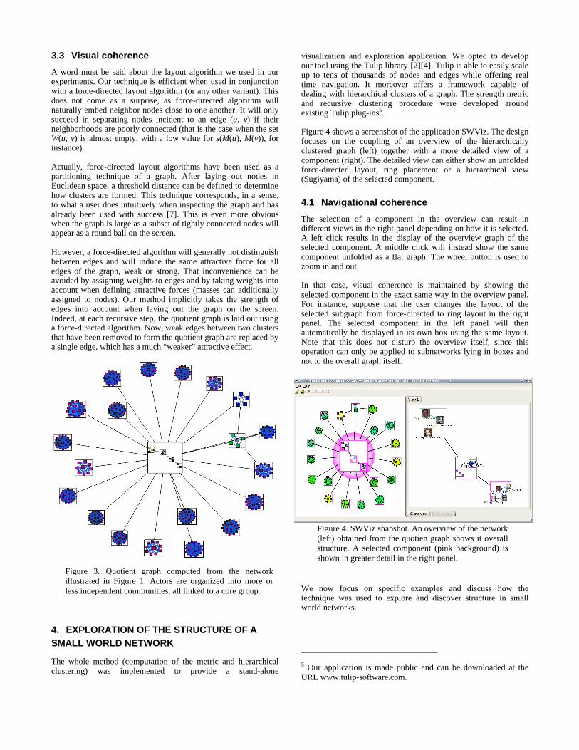
Figure 4 shows a screenshot of the application SWViz. The design focuses on the coupling of an overview of the hierarchically clustered graph (left) together with a more detailed view of a component (right). The detailed view can either show an unfolded force-directed layout, ring placement or a hierarchical view (Sugiyama) of the selected component.

4.1 Navigational coherence

The selection of a component in the overview can result in different views in the right panel depending on how it is selected. A left click results in the display of the overview graph of the selected component. A middle click will instead show the same component unfolded as a flat graph. The wheel button is used to zoom in and out.

In that case, visual coherence is maintained by showing the selected component in the exact same way in the overview panel. For instance, suppose that the user changes the layout of the selected subgraph from force-directed to ring layout in the right panel. The selected component in the left panel will then automatically be displayed in its own box using the same layout. Note that this does not disturb the overview itself, since this operation can only be applied to subnetworks lying in boxes and not to the overall graph itself.

We now focus on specific examples and discuss how the technique was used to explore and discover structure in small world networks.

5 Our application is made public and can be downloaded at the URL www.tulip-software.com.

Figure 3. Quotient graph computed from the network illustrated in Figure 1. Actors are organized into more or less independent communities, all linked to a core group.

Figure 4. SWViz snapshot. An overview of the network (left) obtained from the quotien graph shows it overall structure. A selected component (pink background) is shown in greater detail in the right panel.

4.2 Resyn Assistant API

“Resyn Assistant” is a software designed for the study of chemical components developed in Montpellier (LIRMM). Before going into a new development stage and making new design decisions, the development team decided to study the structure of the actual API. The visualization of the access graph of their API enabled the team to recover the whole history of the past development. Moreover, it offered them a new perspective on their software and showed that their code was organized around a central component (see Figure 5). Components at the periphery correspond to dedicated modules. For instance, classes related to the topology of molecules are grouped into a single cluster. The overall structure of the API is clearly illustrated in Figure 4.

Resyn’s designers were actually able to identify an error in the design of the API. Digging into the hierarchy down to the second level, they found that classes with similar functionalities, that were expected to belong to the same subgroup, were spread out onto two different clusters. The designers plan to recover from this design error in the next release of Resyn.

4.3 IMDB subset

We will now have a closer look at the IMDB subset of actors (Figure 1). The central group in the quotient graph (Figure 3) gathers internationally renowned movie actors, such as Sharon Stone, Meryl Streep, Leonardo Di Caprio, Al Pacino. They lie at the center mainly because of their presence in numerous movies. Clusters at the periphery correspond to movies (actors having played in a same movie necessarily define a clique). This example clearly shows that the method is efficient at finding the influential actors of a small world network.

4.4 Other examples

Many other example graphs extracted from the IMDB were studied. Also, we were able to apply our method to various graphs computed from software systems (include files of Mac OS9, MFC classes, etc.). In each case the method was able to correctly

identify modules or components and showed expected dependencies between them.

5. CHOICE OF THE THRESHOLD VALUE AND QUALITY MEASUREMENTS

One important question has been deferred until now. Just how one should proceed to determine whether an edge is a weak edge ? In other words, how does one choose the threshold value applied to the strength metric when filtering out edges ? A completely satisfying answer to this question requires some work and should rely on the knowledge of the distribution of values for the strength metric.

This is not enough however. Indeed, the choice of the threshold is determined by the fact that the partition induced from the filtering procedure is “good”. So our initial interrogation bounces on the following question: “What is a good partition for a graph ?”. Many criteria have been proposed as strategies for partitioning graphs. In many cases, the partitioning criteria can actually be rephrased as an optimization problem. That is, the “best” partition possible often minimizes a given cost function defined on the set of all possible partitions of a graph. Most of these optimization problems do not admit deterministic solutions however, and many heuristics computing an approaching solution have been proposed. (See [2], [5], [8], for instance.)

5.1 Quality of a partition

The problem of determining the quality of a partition for a given graph can then be answered by computing just how close a partition is to a partition with optimal cost. The answer to this question itself relies on the knowledge of the distribution of costs on the set of all possible partitions.

These considerations led us to select a specific cost function called MQ, first introduced as a partition cost function in the field of software reverse engineering [14]. We provide the definition of MQ, for sake of completeness (see [6]). Given a clustering C={C1, C2, …, Cn} of a graph G, MQ is defined as:

The first term is the mean value of edge density inside each cluster. The second term is the mean value of edge density between the clusters. (See section 3 where the “s” notation is introduced.) It is worth to note that MQ is not a measure for the quality of the visualization itself. It serves as an objective measure of the quality of a clustering (among all possible clustering of the graph).

We apply MQ to automatically choose the “best” clustering for a given graph. The distribution of MQ values (over the set of all partitions of a given graph) is close to a gaussian distribution with µ = -0.2 and σ = 0.2 (MQ is normalized and varies in the [-1, 1] interval). Hence, given any possible MQ value c, we are able to determine the probability for a partition to have a value at least equal to c. For instance, only 0.5% of all partitions of a graph have an MQ value above 0.315. We refer the reader to [6] for more details.

Figure 5. The hierarchical decomposition of the Resyn API shows how the software modules are related to each other.

5.2 Correlating edge strength with MQ

Hence, we see that an answer to our original question of determining the optimal threshold can be based on a combined study of edge strength and MQ. More precisely, the selected threshold should be the one inducing a partition with highest possible MQ value. Figure 6 shows a curve (histogram) describing the variation of MQ with respect to strength. The optimal threshold c = 1.6 can be easily obtained by inspection.

5.2.1 Improving quality

Recall that once a threshold value has been selected, edges with strength below the threshold are discarded. This induces a partition of the graph into several components. In many cases however, this partition will contain several isolated vertices, which actually impoverish its MQ quality. This difficulty can be avoided as follows: isolated vertex with degree one in the original graph are de facto re-inserted in their unique neighbor’s cluster. All other isolated vertices are momentarily grouped into a single cluster and the subgraph induced from this subset is then cut into its connected components.

We were able to observe that this simple reorganization step significantly improves the MQ value associated with a given threshold (by comparing with the results described in [6]). Indeed, post-processing isolated vertices enabled us to reach MQ values as high as 0.8 and 0.9. These values are rather exceptional since a partition has an MQ value at least equal to 0.75 with probability 10-6. Values for Resyn and the IMDB networks are reported in Table 2 below.

Graph (and clustering) MQ Resyn top level quotient 0.771772 Resyn second level quotient (central component in Figure 5) 0.481984

IMDB example network top level quotient 0.947879 IMDB example network second level (right component in Figure 4) 0.6883

Table 2. Listing of several MQ values for the Resyn and IMDB examples. These scores are extremely high and exceptional, considering that MQ is close to a gaussian distribution with µ = -0.2 and σ = 0.2.

5.2.2 A simple partitioning heuristic

Our application takes care of selecting the threshold for the user, by examining the Strength/MQ histogram of a graph. However, one could imagine giving the user complete control over threshold selection by mean of a range slider. This interactive approach has a low computational cost and can be seen as an alternative over other heuristics for many reasons.

§ Many clustering techniques indeed aim at finding partitions having a minimal number of outer edges as possible. This is in accordance with our approach since the filtered out edges indeed correspond to those outer edges. The filtered out edges are “long range” edges, which form a minority of all edges (which can be seen as a property of small world networks).

§ The application provides the user with immediate visual feedback on the partition that is computed, enabling an expert to assess of its significance, e.g.

§ Its computing time is way below the usual optimization algorithms such as hill climbing or genetic algorithms used in software dedicated to graph clustering.

§ But most of all, the validity of these arguments rely on the fact that our method is able to find partitions with an exceptionally high MQ value, which assess of its acuity.

6. CONCLUSION AND FUTURE WORK

Many other application domains must be studied, and many more data set need to be collected and analyzed in order to establish the relevance of small world networks in Information Visualization. Application domains such as biology (neural networks) and linguistics (word association) offer fertile grounds that should be investigated more closely.

We are currently extending our application with navigation techniques such as semantic fish-eye. This will allow the user to navigate the hierarchical network from and into a single panel since the fish-eye combines detailed information and overall context.

A closer examination of structural properties of small world networks such as degree distribution could help us design specific visual cues. Also, the criteria from which small world networks are defined should be revised from an information visualization perspective in order to straighten the vagueness of the statement “having a clustering index significantly higher than a random graph”. Indeed, many examples we looked at and that complied best with our approach had relatively high clustering index (often up to 95%). This calls for the definition of a more focused class of small world networks that differ from some theoretical constructions and correspond better to real-life examples.

References

[1] ADAMIC, L.A. The Small World Web, Xerox Palo Alto Research Center.

[2] ALPERT, C.J. AND A.B. KAHNG. 1995. Recent Developments in Netlist Partitioning: A Survey. Integration: the VLSI Journal 19, 1-2, 1-81.

Figure 6. The curve describes the variation of MQ with respect to edge strength for the “Resyn Assistant” API. The “optimal” threshold approaches 1.6 with for MQvalue close to 0.80, which is remarkably high.

[3] AUBER, D. 2001. Tulip. In 9th International Symposium on Graph Drawing, GD 2001. Lecture Notes in Computer Science 2265, Springer-Verlag. Vienna, Austria.

[4] AUBER, D. 2003. Tulip - A huge graph visualization framework, in Graph Drawing Software. P. Mutzel and M. Jünger, editors. Springer Verlag.

[5] BERKHIN, P. 2002. Survey Of Clustering Data Mining Techniques. Accrue Software: San Jose, CA.

[6] CHIRICOTA, Y., F. JOURDAN, AND G. MELANÇON. 2003. Software Components Capture using Graph Clustering. In: 11th IEEE International Workshop on Program Comprehension. Portland, Oregon: IEEE / ACM.

[7] FAIRCHILD, K.M., S.E. POLTROCK, AND G.W. FURNAS. 1988. SemNet: Three-Dimensional Representation of Large Knowledge Bases. In Cognitive Science and Its Applications for Human-Computer Interaction. Lawrence Erlbaum Associates, Inc.

[8] FJÄLLSTROM, P. 1998. Algorithms for graph partitioning: A survey. Linkoping Electronic Articles in Computer and Information Science, 3.

[9] GUARE, J. 1990. Six degrees of Separation: A Play. New York: Vintage Books.

[10] KASTURIRANGAN, R. 1999. Multiple Scales in Small-World Networks. Brain and Cognitive Science Department, MIT.

[11] KLEINBERG, J. 2000. The Small-World Phenomenon: An Algorithmic Perspective. In: 32nd ACM Symposium on Theory of Computing.

[12] FREEMAN, L.C. 2000. Visualizing Social Networks. Journal of Social Structures 1, 1. http://www2.heinz.cmu.edu/project/INSNA/joss/.

[13] MILGRAM, S. 1967. The small world problem. Psychology Today 1, 61.

[14] MITCHELL, B.S., MANCORIDIS S., YIH-FARN C., GANSNER E. 1999. Bunch: A Clustering Tool for the Recovery and Maintenance of Software System Structures. In: International Conference on Software Maintenance, ICSM.

[15] NEWMAN, M., WATTS D., AND STROGATZ S.H., Random graph models of social networks. Proceedings of the National Academy of Sciences. To appear.

[16] SHNEIDERMAN, B. 1996. The Eyes Have It: A Task by Data Type Taxonomy for Information Visualization. In IEEE Conference on Visual Languages (VL'96). Boulder, CO: IEEE CS Press.

[17] WATTS, D.J. 1999. Small Worlds. Princeton University Press.

[18] WATTS, D.J. AND STROGATZ S.H. 1998. Collective dynamics of "small-world" networks. Nature 393, 440-442.