Potomac Aquifer System, SWIFT Research Center - VTechWorks
160
Groundwater Modeling and Hydrogeological Parameter Estimation: Potomac Aquifer System, SWIFT Research Center Eric D. Matynowski Thesis submitted to the faculty of the Virginia Polytechnic Institute and State University in partial fulfillment of the requirements for the degree of Master of Science In Environmental Engineering Mark A. Widdowson, Chair Thomas J. Burbey Erich T. Hester May 19, 2020 Blacksburg, Virginia Keywords: Groundwater Model, Travel Times, Multi-layered Aquifer, Hydrogeological Parameters
-
Upload
khangminh22 -
Category
Documents
-
view
0 -
download
0
Transcript of Potomac Aquifer System, SWIFT Research Center - VTechWorks

Groundwater Modeling and Hydrogeological Parameter Estimation:
Potomac Aquifer System, SWIFT Research Center
Eric D. Matynowski
Thesis submitted to the faculty of the Virginia Polytechnic Institute and State University
in partial fulfillment of the requirements for the degree of
Master of Science
In
Environmental Engineering
Mark A. Widdowson, Chair
Thomas J. Burbey
Erich T. Hester
May 19, 2020
Blacksburg, Virginia
Keywords: Groundwater Model, Travel Times, Multi-layered Aquifer, Hydrogeological
Parameters

Groundwater Modeling and Hydrogeological Parameter Estimation:
Potomac Aquifer System, SWIFT Research Center
Eric D. Matynowski
Abstract
The Sustainable Water Interactive for Tomorrow (SWIFT) project in eastern Virginia is a
Managed Aquifer Recharge project designed to alleviate the depletion of the Potomac
Aquifer System due to unsustainable groundwater withdrawals. At the SWIFT Research
Center (SWIFTRC) in Nansemond, VA, a pilot testing well (TW-1) has been implemented
to help determine the feasibility of full-scale implementation. The pumping data from TW-
1 and observation head data from surrounding monitoring wells (MW) at the SWIFTRC
were used to calculate hydrogeological parameters (transmissivity, hydraulic conductivity,
specific storage, and storage coefficients). Two sets of data were analyzed from before and
after TW-1 was rehabilitated to account for the change in the flow distribution to each
screen in TW-1. Comparing the results to past literature, the calculated (Theis and Cooper-
Jacob methods) hydraulic conductivity/transmissivity values are within the same order of
magnitude. Using borehole logs as well as apparent conductance and resistivity logs,
multiple single and multi-layered models for both the upper and middle Potomac aquifers
were produced with MODFLOW. Parameter estimation using MODFLOW and PEST and
the two sets of observation data resulted in hydrogeological parameters similar to those
calculated using Theis and Cooper-Jacob methods. The change in the hydraulic
conductivity and specific storage between the pre and post rehabilitation flow distributions
is proportional to that change in the flow distribution. For future modeling of the aquifer
system, the hydrogeological parameters from the model using the 4/26/19 data set with the
post rehabilitation flow distribution is recommended.
Drawdown results from a multi-layered MODFLOW model were compared to results using
the Theis method using both the Theis-calculated and MODFLOW-PEST modeled
hydrogeological parameters. The results were nearly identical except for the Upper
Potomac Aquifer (UPA) layer 1, as the model has a large change in aquifer thickness with
distance from TW-1 that the Theis-based calculations do not consider.
Travel times from the monitoring wells to TW-1 were calculated with the single and multi-
layered models pumping 700 GPM from TW-1. Travel times from the SWIFT MW within
the UPA sublayers ranged from 204 to 597 days depending on the sublayer, while travel
times from the USGS MW within the UPA sublayers ranged from 2,395 to 7,859 days.
For the single layer model of the UPA, the travel time from the SWIFT MW to TW-1 was
372 days while the travel time from the USGS MW was 4,839 days. Travel times from the
SWIFT MW within the MPA sublayers were 416 and 1,195 days, while travel times from
the USGS MW within the MPA sublayers were 4,339 and 11,245 days. For the single
layer model of the MPA, the travel time from the SWIFT MW to TW-1 was 743 days while
the travel time from the USGS MW was 7,545 days.
Groundwater Modeling and Hydrogeological Parameter Estimation:
Potomac Aquifer System, SWIFT Research Center
Eric D. Matynowski
General Audience Abstract
The Sustainable Water Interactive for Tomorrow (SWIFT) project in eastern Virginia is a
project designed to help slow the depletion of the Potomac Aquifer System due to
unsustainable groundwater withdrawals. At the SWIFT Research Center (SWIFTRC) in
Nansemond, VA, a testing well (TW-1) has been implemented to help determine if the full-
scale implementation of the SWIFT project is feasible. The pumping data from TW-1 and
observation head data from surrounding monitoring wells (MW) at the SWIFTRC were
used to calculate hydrogeological parameters (transmissivity, hydraulic conductivity,
specific storage, and storage coefficients). These parameters help describe the behavior of
the aquifer system. Two sets of data were analyzed from before and after TW-1 was
rehabilitated to account for the change in the flow distribution within TW-1. Comparing
the results to past literature, the calculated (using analytical methods, Theis and Cooper-
Jacob methods) hydraulic conductivity/transmissivity values are within the same order of
magnitude. Using data from the boreholes, multiple single and multi-layered models for
both the upper and middle Potomac aquifers were produced with MODFLOW, a
groundwater modeling software. Estimating parameters using observation data within
MODFLOW resulted in hydrogeological parameters similar to those calculated using the
Theis and Cooper-Jacob methods. The change in the hydraulic conductivity and specific
storage between the pre and post rehabilitation flow distributions within TW-1 is
proportional to that change in the flow distribution. For future modeling of the aquifer
system, the hydrogeological parameters from the model using the 4/26/19 (most recent)
data set with the post rehabilitation (more current) flow distribution is recommended.
Drawdown (decrease in the water table) results from a multi-layered MODFLOW model
were compared to results using the Theis method using both the Theis-calculated and

MODFLOW modeled hydrogeological parameters. The results were nearly identical
except for the Upper Potomac Aquifer (UPA) layer 1, as the model has a large change in
aquifer thickness with distance from TW-1 that the Theis-based calculations do not
consider.
The time it took for a particle of water to travel from the monitoring wells to TW-1 were
calculated with the single and multi-layered models pumping 700 GPM from TW-1.
Travel times from the SWIFT MW within the UPA sublayers ranged from 204 to 597 days
depending on the sublayer, while travel times from the USGS MW within the UPA
sublayers ranged from 2,395 to 7,859 days. For the single layer model of the UPA, the
travel time from the SWIFT MW to TW-1 was 372 days while the travel time from the
USGS MW was 4,839 days. Travel times from the SWIFT MW within the MPA sublayers
were 416 and 1,195 days, while travel times from the USGS MW within the MPA sublayers
were 4,339 and 11,245 days. For the single layer model of the MPA, the travel time from
the SWIFT MW to TW-1 was 743 days while the travel time from the USGS MW was
7,545 days.

vi
Acknowledgement
I would first like to thank my adviser, Dr. Mark Widdowson, for everything he has done to help
me through graduate school and for providing guidance with my research. Even with his busy
schedule, he made sure to make time not just to help me, but all his students. His work ethic and
willingness to help is truly inspiring. I would also like to thank my committee members, Dr. Hester
and Dr. Burbey for helping me with this process. I would also like to thank Meredith Ballard for
her help with providing important knowledge and data that was needed to complete this research
and for her willingness to take time from her own work to help me with mine.
I next want to thank all the great colleagues and faculty members at the EWR graduate program at
Virginia Tech for their support and friendship. Although graduate school was challenging and
stressful at times, they helped lift me up and make it an enjoyable experience.
Finally, I would like to thank my friends and family for all their love and support. My parents and
my brother are always there for me and provide an endless amount of love and support for me and
I am so grateful for that. I would also like to thank my friend Matt for being there for me when I
need it and for listening while I vent my stress. Lastly, I would like to thank Maddie for her love
and support, I could not have done this without you.
vii
Table of Contents
Abstract ........................................................................................................................................... ii General Audience Abstract ............................................................................................................ iv Acknowledgement ......................................................................................................................... vi Table of Contents .......................................................................................................................... vii
List of Figures ................................................................................................................................ ix List of Tables ............................................................................................................................... xiv Abbreviations .............................................................................................................................. xvii 1 Introduction ............................................................................................................................. 1
Background ...................................................................................................................... 1
Study Area ........................................................................................................................ 3
Purpose and Scope ........................................................................................................... 4 2 Literature Review.................................................................................................................... 5
Managed Aquifer Recharge ............................................................................................. 5
Why Utilize MAR ..................................................................................................... 5
MAR Types ............................................................................................................... 5
MAR Modeling ................................................................................................................ 6 Scale .......................................................................................................................... 6
Time and Space Discretization ................................................................................. 7
Travel Time ............................................................................................................... 7
Hydrogeological Parameters – Previous Studies ............................................................. 8
3 Data Sources ......................................................................................................................... 11
Wells............................................................................................................................... 11 Well Screening ........................................................................................................ 11
Well Data Sets......................................................................................................... 13
Flow Distribution at TW-1 ............................................................................................. 15 Borehole Data for SWIFT Monitoring Wells ................................................................ 17
4 Methods and Model Description ........................................................................................... 18
Layer Definition ............................................................................................................. 18 Direction and Gradient of Pre-MAR Flow ..................................................................... 23 Hydrogeological Parameters .......................................................................................... 26 GMS/MODFLOW ......................................................................................................... 31
Modeling Assumptions .................................................................................................. 32 GMS Base Models ......................................................................................................... 33 Single Layer Models and Parameter Estimation ............................................................ 40
Multi-Layered Aquifer Models ...................................................................................... 44 Estimating Drawdown within the Multi-Layered Models Using Theis Method .... 48
Estimating Drawdown within the Multi-Layered Models Using MODFLOW ...... 49
Estimating Travel Times within the Single and Multi-Layered Models ........................ 51 5 Results and Discussion ......................................................................................................... 54
Pump Test Analysis with Theis and Cooper-Jacob Methods ......................................... 54

viii
GMS Model Results ....................................................................................................... 57
Hydrogeological Parameter Estimation .................................................................. 57
Multi-Layered Drawdown ...................................................................................... 65
Travel Times ........................................................................................................... 70
6 Conclusion ............................................................................................................................ 72 Summary ........................................................................................................................ 72 Study Limitations and Future Work ............................................................................... 73
References ..................................................................................................................................... 74 ................................................................................................................................... 79

ix
List of Figures
Figure 1-1. Depiction of the PAS cross section throughout the VCPPP (Nelms et al., 2003). ...................... 1
Figure 1-2. Map of the region surrounding the site for this research (outlined in red) with city names for
reference. ...................................................................................................................................................... 3
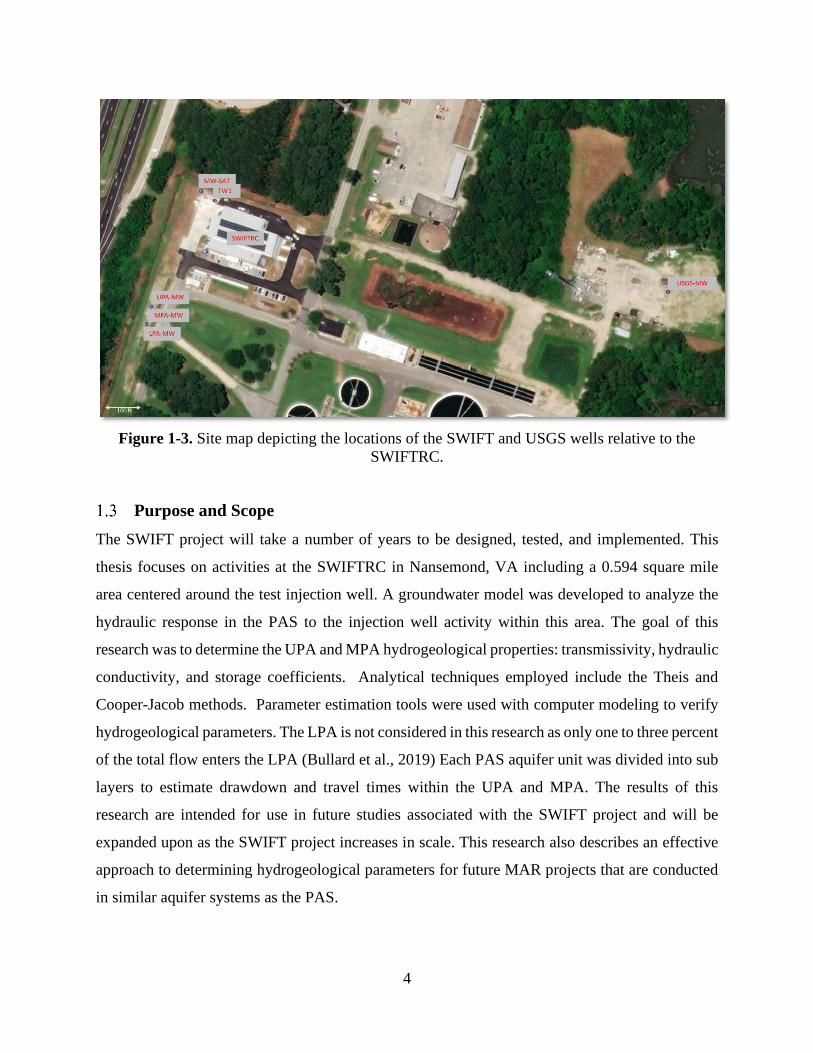
Figure 1-3. Site map depicting the locations of the SWIFT and USGS wells relative to the SWIFTRC. ......... 4
Figure 2-1. Map of the Potomac aquifer system displaying the estimated range of transmissivity values
(Trapp Jr. & Horn, 1997). .............................................................................................................................. 9
Figure 2-2. Map of the estimated range for the hydraulic conductivity values for the Potomac aquifer
(Heywood & Pope, 2009). ........................................................................................................................... 10
Figure 3-1. Conceptual cross section model of the SWIFT wells depicting the aquifer layers, the well
depths, the screening for each well, and the distance each MW is from TW-1 (SWIFT & USGS, 2018). .. 12
Figure 4-1. Conceptual model of the PAS beneath the SWIFTRC showing both the aquifer and confining
layered that make up the UPA, MPA, and LPA ........................................................................................... 18
Figure 4-2. Soil type with depth at TW-1 with the screened intervals and hydrologic units (Lucas, 2016).
.................................................................................................................................................................... 20
Figure 4-3. Location of the cross section depicting the GMS solid layering of both the high- and low-
resolution models for both the UPA and MPA. .......................................................................................... 22
Figure 4-4. Cross section through the low resolution (single layered) UPA and MPA GMS model. .......... 22
Figure 4-5. Cross section through the high resolution (Multiple layers) UPA and MPA GMS model. ....... 23
Figure 4-6. Satellite map of the region with the locations of each well used to calculate the direction and
gradient of flow along with the two triangles they form. .......................................................................... 24
Figure 4-7. Drawdown vs time for the UPA-MW with the 8/18 data set overlayed on the W(u) vs 1/u
graph used for the Theis method. .............................................................................................................. 29
Figure 4-8. Drawdown vs time on a log scale for the UPA-MW with the 8/18 data set used for the
Cooper-Jacob method. ................................................................................................................................ 30
Figure 4-9. GMS model of the research site depicting the aquifer layers and the wells used. .................. 32
Figure 4-10. Aerial satellite map of the research site with the red outline showing the domain of the
model. ......................................................................................................................................................... 34
Figure 4-11. Model domain with the location of TW-1 and the TIN mesh. ................................................ 35
Figure 4-12. Depiction of the two coverage types with the red showing the nodes, arcs, and polygons
used to specify hydrogeological parameters. Blue shows the wells used for observation data,
refinement, and pumping flow rates. ......................................................................................................... 37
Figure 4-13. Depiction of model grid centered and refined around TW-1. Zoomed in to better show cell
sizing. .......................................................................................................................................................... 39
Figure 4-14. 3D depiction of the UPA domain with the aquifer divided into multiple sublayers. ............ 45
Figure 4-15. 3D depiction of the MPA domain with the aquifer divided into multiple sublayers. ............ 45
Figure 4-16. Travel time path lines from the UPA-MW and the USGS-MW to TW-1 (From the 8/18 pre-
flow UPA multi-layered model). ................................................................................................................. 53
Figure 5-1. Sensitivity of the estimated parameters within the 8/18 pre-flow UPA single layer model
using PEST (1-2). .......................................................................................................................................... 59
Figure 5-2. Sensitivity of the estimated parameters within the 4/19 post flow MPA single layer model
using PEST (2-13). ........................................................................................................................................ 59

x
Figure 5-3. Sensitivity of the estimated parameters within the 8/18 pre-flow MPA single layer model
using PEST (2-2). .......................................................................................................................................... 59
Figure 5-4. Modeled cone of influence at the end of one day of pumping for the UPA model run utilizing
the 8/18 data set and the pre-rehabilitation flow distribution. ................................................................. 60
Figure 5-5. Modeled cone of influence at the end of one day of pumping for the MPA model run utilizing
the 8/18 data set and the pre-rehabilitation flow distribution. ................................................................. 61
Figure 5-6. Modeled hydraulic conductivity values from the models only using the SWIFT MW
observation data vs the averaged calculated hydraulic conductivity of the Theis and Cooper-Jacob
methods with a one to one line for comparison. ....................................................................................... 66
Figure 5-7. Modeled cone of depression showing the impact pumping at TW-1 has on the aquifer system
after one day of pumping. (From UPA L1 of the 8/18 pre-flow UPA multi-layered model). ...................... 67
Figure 5-8. Final drawdown after one day of pumping for the results from the UPA multi-layered model’s
vs the calculated drawdown layered UPA with the Theis method. A one to one line is provided for
comparison. ................................................................................................................................................ 68
Figure 5-9. Final drawdown after one day of pumping for the results from the MPA multi-layered
model’s vs the calculated drawdown layered MPA with the Theis method. A one to one line is provided
for comparison. ........................................................................................................................................... 68
Figure 5-10. Drawdown over one day of the UPA L1 for the UPA 8/18 pre-flow model. .......................... 69
Figure 5-11. Drawdown over one day of the UPA L1 for the UPA 4/19 post flow model. ......................... 69
Figure 5-12. Drawdown over one day of the UPA L2 for the UPA 8/18 pre-flow model. .......................... 69
Figure 5-13. Drawdown over one day of the UPA L2 for the UPA 4/19 post flow model. ......................... 69
Figure 5-14. Drawdown over one day of the UPA L3 for the UPA 8/18 pre-flow model. .......................... 69
Figure 5-15. Drawdown over one day of the UPA L3 for the UPA 4/19 post flow model. ......................... 69
Figure 5-16. Drawdown over one day of the MPA L1 for the UPA 8/18 pre-flow model. ......................... 69
Figure 5-17. Drawdown over one day of the MPA L1 for the UPA 4/19 post flow model. ........................ 69
Figure 5-18. Drawdown over one day of the MPA L2 for the UPA 8/18 pre-flow model. ......................... 70
Figure 5-19. Drawdown over one day of the MPA L2 for the UPA 4/19 post flow model. ........................ 70
Figure A-1. Change in depth to water level for the flute well screens during the 8/3/18 data set. .......... 79
Figure A-2. Change in depth to water level for the flute well screens during the 4/26/19 data set. ........ 79
Figure A-3. Resitivity per foot of depth for the USGS wells used to determine layer definition. .............. 80
Figure A-4. Apparent conductance per foot of depth for the USGS wells used to determine layer
definition. .................................................................................................................................................... 81
Figure A-5. TW-1 borehole log, with information like the wells, location, date drilled, diameter, and soil
type with depth. (includes the next 6 pages). ............................................................................................ 83
Figure A-6. Flute well borehole log, with information like the wells, location, date drilled, diameter, and
soil type with depth. (includes the next 6 pages). ...................................................................................... 89
Figure A-7. UPA-MW borehole log, with information like the wells, location, date drilled, diameter, and
soil type with depth. (includes the next 4 pages). ...................................................................................... 95
Figure A-8. MPA-MW borehole log, with information like the wells, location, date drilled, diameter, and
soil type with depth. (includes the next 4 pages). ...................................................................................... 99
Figure A-9. LPA-MW borehole log, with information like the wells, location, date drilled, diameter, and
soil type with depth. (includes the next 5 pages). .................................................................................... 103
Figure A-10. Schematic of wells used to determine hydraulic gradient magnitude and direction with
angle and triangle labeled......................................................................................................................... 108

xi
Figure A-11. Schematic of right-angle triangle between wells 58C 58 and 59D 36 used in hydraulic
gradient magnitude and direction calculations. ....................................................................................... 108
Figure A-12. 8/18 UPA-MW: figure contains data set used for Theis and Cooper-Jacob calculations. W(u)
vs 1/u overlayer on drawdown vs time graph for Theis method. Drawdown vs time on a log scale for the
Cooper-Jacob method. The Parameters used and results found with the Theis method with the pre and
post flow distribution. The Parameters used and results found with the Cooper-Jacob method with both
the pre and post flow distribution. Light green data are the data used for the linear line for the Cooper-
Jacob method and the dark green are the two points used for the Cooper-Jacob calculations. ............. 110
Figure A-13. 8/18 USGS-UPA: figure contains data set used for Theis and Cooper-Jacob calculations.
W(u) vs 1/u overlayer on drawdown vs time graph for Theis method. Drawdown vs time on a log scale
for the Cooper-Jacob method. The Parameters used and results found with the Cooper-Jacob method
with both the pre and post flow distribution. Light green data are the data used for the linear line for the
Cooper-Jacob method and the dark green are the two points used for the Cooper-Jacob calculations. 111
Figure A-14. 8/18 MPA-MW: figure contains data set used for Theis and Cooper-Jacob calculations. W(u)
vs 1/u overlayer on drawdown vs time graph for Theis method. Drawdown vs time on a log scale for the
Cooper-Jacob method. The Parameters used and results found with the Theis method with the pre and
post flow distribution. The Parameters used and results found with the Cooper-Jacob method with both
the pre and post flow distribution. Light green data are the data used for the linear line for the Cooper-
Jacob method and the dark green are the two points used for the Cooper-Jacob calculations. ............. 112
Figure A-15. 8/18 USGS-MPA: figure contains data set used for Theis and Cooper-Jacob calculations.
W(u) vs 1/u overlayer on drawdown vs time graph for Theis method. Drawdown vs time on a log scale
for the Cooper-Jacob method. Light green data are the data used for the linear line for the Cooper-Jacob
method. ..................................................................................................................................................... 113
Figure A-16. 4/19 UPA-MW: figure contains data set used for Theis and Cooper-Jacob calculations. W(u)
vs 1/u overlayer on drawdown vs time graph for Theis method. Drawdown vs time on a log scale for the
Cooper-Jacob method. The Parameters used and results found with the Theis method with the pre and
post flow distribution. The Parameters used and results found with the Cooper-Jacob method with both
the pre and post flow distribution. Light green data are the data used for the linear line for the Cooper-
Jacob method and the dark green are the two points used for the Cooper-Jacob calculations. ............. 114
Figure A-17. 4/19 USGS-UPA: figure contains data set used for Theis and Cooper-Jacob calculations.
W(u) vs 1/u overlayer on drawdown vs time graph for Theis method. Drawdown vs time on a log scale
for the Cooper-Jacob method. .................................................................................................................. 115
Figure A-18. 4/19 MPA-MW: figure contains data set used for Theis and Cooper-Jacob calculations. W(u)
vs 1/u overlayer on drawdown vs time graph for Theis method. Drawdown vs time on a log scale for the
Cooper-Jacob method. The Parameters used and results found with the Theis method with the pre and
post flow distribution. The Parameters used and results found with the Cooper-Jacob method with both
the pre and post flow distribution. Light green data are the data used for the linear line for the Cooper-
Jacob method and the dark green are the two points used for the Cooper-Jacob calculations. ............. 116
Figure A-19. 4/19 USGS-MPA: figure contains data set used for Theis and Cooper-Jacob calculations.
W(u) vs 1/u overlayer on drawdown vs time graph for Theis method. Drawdown vs time on a log scale
for the Cooper-Jacob method. The Parameters used and results found with the Theis method with the
pre and post flow distribution. The Parameters used and results found with the Cooper-Jacob method
with both the pre and post flow distribution. Light green data are the data used for the linear line for the
Cooper-Jacob method and the dark green are the two points used for the Cooper-Jacob calculations. 117
xii
Figure A-20. Sensitivity of the estimated parameters within the 8/18 post flow UPA single layer model
using PEST. ................................................................................................................................................ 123
Figure A-21. Sensitivity of the estimated parameters within the 4/19 pre-flow UPA single layer model
using PEST. ................................................................................................................................................ 123
Figure A-22. Sensitivity of the estimated parameters within the 4/19 post flow UPA single layer model
using PEST. ................................................................................................................................................ 123
Figure A-23. Sensitivity of the estimated parameters within the 8/18 post flow MPA single layer model
using PEST. ................................................................................................................................................ 123
Figure A-24. Sensitivity of the estimated parameters within the 4/19 pre-flow MPA single layer model
using PEST. ................................................................................................................................................ 123
Figure A-25. Modeled vs observed change in head for both the SWIFT MW and the USGS MW for the
UPA, 8/18 pre-rehab flow with equal weighting for each observation point. ......................................... 126
Figure A-26. Modeled vs observed change in head for both the SWIFT MW and the USGS MW for the
UPA, 8/18 pre-rehab flow with a weighting of 1 for USGS MW and 4 for the SWIFT MW. ..................... 126
Figure A-27. Modeled vs observed change in head for both the SWIFT MW and the USGS MW for the
UPA, 8/18 pre-rehab flow with a weighting of 1 for the SWIFT MW and no SWIFT MW. ....................... 127
Figure A-28. Modeled vs observed change in head for both the SWIFT MW and the USGS MW for the
UPA, 8/18 post rehab flow with equal weighting for each observation point. ........................................ 127
Figure A-29. Modeled vs observed change in head for both the SWIFT MW and the USGS MW for the
UPA, 8/18 post rehab flow with a weighting of 1 for USGS MW and 4 for the SWIFT MW. .................... 128
Figure A-30. Modeled vs observed change in head for both the SWIFT MW and the USGS MW for the
UPA, 8/18 post rehab flow with a weighting of 1 for the SWIFT MW and no SWIFT MW. ...................... 128
Figure A-31. Modeled vs observed change in head for both the SWIFT MW and the USGS MW for the
UPA, 4/19 pre-rehab flow using the hydrogeological parameters from the UPA, 8/18 pre-rehab flow
model with a weighting of 1 for USGS MW and 4 for the SWIFT MW. .................................................... 129
Figure A-32. Modeled vs observed change in head for both the SWIFT MW and the USGS MW for the
UPA, 4/19 pre-rehab flow with equal weighting for each observation point. ......................................... 129
Figure A-33. Modeled vs observed change in head for both the SWIFT MW and the USGS MW for the
UPA, 4/19 pre-rehab flow with a weighting of 1 for USGS MW and 4 for the SWIFT MW. ..................... 130
Figure A-34. Modeled vs observed change in head for both the SWIFT MW and the USGS MW for the
UPA, 4/19 pre-rehab flow with a weighting of 1 for the SWIFT MW and no SWIFT MW. ....................... 130
Figure A-35. Modeled vs observed change in head for both the SWIFT MW and the USGS MW for the
UPA, 4/19 post rehab flow using the hydrogeological parameters from the UPA, 8/18 post rehab flow
model with a weighting of 1 for USGS MW and 4 for the SWIFT MW. .................................................... 131
Figure A-36. Modeled vs observed change in head for both the SWIFT MW and the USGS MW for the
UPA, 8/18 pre-rehab flow with equal weighting for each observation point. ......................................... 131
Figure A-37. Modeled vs observed change in head for both the SWIFT MW and the USGS MW for the
UPA, 4/19 post rehab flow with a weighting of 1 for USGS MW and 4 for the SWIFT MW. .................... 132
Figure A-38. Modeled vs observed change in head for both the SWIFT MW and the USGS MW for the
UPA, 4/19 post rehab flow with a weighting of 1 for the SWIFT MW and no SWIFT MW. ...................... 132
Figure A-39. Modeled vs observed change in head for both the SWIFT MW and the USGS MW for the
MPA, 8/18 pre-rehab flow with equal weighting for each observation point. ........................................ 133
Figure A-40. Modeled vs observed change in head for both the SWIFT MW and the USGS MW for the
MPA, 8/18 pre-rehab flow with a weighting of 1 for USGS MW and 4 for the SWIFT MW. .................... 133
xiii
Figure A-41. Modeled vs observed change in head for both the SWIFT MW and the USGS MW for the
MPA, 8/18 pre-rehab flow with a weighting of 1 for the SWIFT MW and no SWIFT MW. ...................... 134
Figure A-42. Modeled vs observed change in head for both the SWIFT MW and the USGS MW for the
MPA, 8/18 post rehab flow with equal weighting for each observation point. ....................................... 134
Figure A-43. Modeled vs observed change in head for both the SWIFT MW and the USGS MW for the
MPA, 8/18 post rehab flow with a weighting of 1 for USGS MW and 4 for the SWIFT MW. ................... 135
Figure A-44. Modeled vs observed change in head for both the SWIFT MW and the USGS MW for the
MPA, 8/18 post rehab flow with a weighting of 1 for the SWIFT MW and no SWIFT MW. ..................... 135
Figure A-45. Modeled vs observed change in head for both the SWIFT MW and the USGS MW for the
MPA, 4/19 pre-rehab flow using the hydrogeological parameters from the MPA, 8/18 pre-rehab flow
model with a weighting of 1 for USGS MW and 4 for the SWIFT MW. .................................................... 136
Figure A-46. Modeled vs observed change in head for both the SWIFT MW and the USGS MW for the
MPA, 4/19 pre-rehab flow with equal weighting for each observation point. ........................................ 136
Figure A-47. Modeled vs observed change in head for both the SWIFT MW and the USGS MW for the
MPA, 4/19 pre-rehab flow with a weighting of 1 for USGS MW and 4 for the SWIFT MW. .................... 137
Figure A-48. Modeled vs observed change in head for both the SWIFT MW and the USGS MW for the
MPA, 4/19 pre-rehab flow with a weighting of 1 for the SWIFT MW and no SWIFT MW. ...................... 137
Figure A-49. Modeled vs observed change in head for both the SWIFT MW and the USGS MW for the
MPA, 4/19 post rehab flow using the hydrogeological parameters from the MPA, 8/18 post rehab flow
model with a weighting of 1 for USGS MW and 4 for the SWIFT MW. .................................................... 138
Figure A-50. Modeled vs observed change in head for both the SWIFT MW and the USGS MW for the
MPA, 4/19 post rehab flow with equal weighting for each observation point. ....................................... 138
Figure A-51. Modeled vs observed change in head for both the SWIFT MW and the USGS MW for the
MPA, 4/19 post rehab flow with a weighting of 1 for USGS MW and 4 for the SWIFT MW. ................... 139
Figure A-52. Modeled vs observed change in head for both the SWIFT MW and the USGS MW for the
MPA, 4/19 post rehab flow with a weighting of 1 for the SWIFT MW and no SWIFT MW. ..................... 139
Figure A-53. Drawdown over one day of the UPA L1 for the UPA 8/18 post flow model. ....................... 142
Figure A-54. Drawdown over one day of the UPA L1 for the UPA 4/19 pre-flow model. ........................ 142
Figure A-55. Drawdown over one day of the UPA L2 for the UPA 8/18 post flow model. ....................... 142
Figure A-56. Drawdown over one day of the UPA L2 for the UPA 4/19 pre-flow model. ........................ 142
Figure A-57. Drawdown over one day of the UPA L3 for the UPA 8/18 post flow model. ....................... 142
Figure A-58. Drawdown over one day of the UPA L3 for the UPA 4/19 pre-flow model. ........................ 142
Figure A-59. Drawdown over one day of the MPA L1 for the UPA 8/18 post flow model. ...................... 142
Figure A-60. Drawdown over one day of the MPA L1 for the UPA 4/19 pre-flow model. ....................... 142
Figure A-61. Drawdown over one day of the MPA L2 for the UPA 8/18 post flow model. ...................... 143
Figure A-62. Drawdown over one day of the MPA L2 for the UPA 4/19 pre-flow model. ....................... 143
xiv
List of Tables
Table 2-1. Estimated hydraulic conductivity values for the aquifer and confining units of the Potomac
aquifer (Smith, 1999). ................................................................................................................................... 8
Table 2-2. Estimated transmissivity values for the upper, middle, and lower Potomac aquifer based on a
packer test (Lucas, 2016). ........................................................................................................................... 10
Table 3-1. Well data used for modeling in this study, such as Well I.D., well elevation, well operator, data
type and aquifer being monitored. ............................................................................................................. 11
Table 3-2. TW-1 well screens including depths, lengths, and aquifer unit. ................................................ 13
Table 3-3. SWIFT UPA monitoring well screens including depths, lengths, and aquifer unit. ................... 13
Table 3-4. SWIFT MPA monitoring well screens including depths, lengths, and aquifer unit.................... 13
Table 3-5. SWIFT LPA monitoring well screens including depths, lengths, and aquifer unit. .................... 13
Table 3-6. TW-1 flow distribution at each screen prior to well rehabilitation (Bullard et al., 2019). ........ 15
Table 3-7. TW-1 flow distribution at each screen following to well rehabilitation (M. Martinez, personal
communication, December 3, 2019). ......................................................................................................... 16
Table 3-8. Flow rates from each aquifer layer for both the 8/18 and 4/19 data sets using the pre-
rehabilitation flow distribution. .................................................................................................................. 16
Table 3-9. Flow rates from each aquifer layer for both the 8/18 and 4/19 data sets using the post
rehabilitation flow distribution. .................................................................................................................. 16
Table 4-1. Wells used to determine the direction and gradient of flow along with the location, depths,
elevations, and head values. ....................................................................................................................... 25
Table 4-2. Distances in the X and Y direction from well 59D 36 for wells used to calculate hydraulic
gradient magnitude and direction. ............................................................................................................. 26
Table 4-3. Intermediate and final calculations for the hydraulic gradient magnitude (I) and direction (𝜃)
for both triangles. ....................................................................................................................................... 26
Table 4-4. Model runs implemented to determine hydrogeological parameters utilizing parameter
estimation, while forward model runs compared results using hydrogeological parameters from 8/18
model runs to 4/19 data sets.. .................................................................................................................... 41
Table 4-5. Model iterations to determine the optimal multiplier and the optimal number of time steps.
.................................................................................................................................................................... 42
Table 4-6. Flow rate values entered into GMS at TW-1 for the 8/18 data set for the UPA and MPA. ....... 43
Table 4-7. Flow rate values entered into GMS at TW-1 for the 4/19 data set for the UPA and MPA. ....... 43
Table 4-8. Estimated transmissivity and specific storage values from Models 1 and 2 based on the SWIFT
MW’s observation data only. ...................................................................................................................... 46
Table 4-9. Aquifer sublayer location of TW-1 screens. ............................................................................... 46
Table 4-10. Pre and post rehabilitation flow distributions for both the UPA and the MPA for both the
8/18 and 4/19 data sets. ............................................................................................................................. 47
Table 4-11. Pre and post rehabilitation flow rate data for both the 8/18 and 4/19 data sets for each
sublayer of the multi-layered models. ........................................................................................................ 47
Table 4-12. Calculated transmissivity and hydraulic conductivity values for the sublayers of both the UPA
and MPA. ..................................................................................................................................................... 48
Table 4-13. Storage coefficient and specific storage data for both the 8/18 and 4/19 data sets for each
sublayer for both the UPA and MPA. .......................................................................................................... 48
xv
Table 4-14. MODFLOW model runs focusing on estimating drawdown in the multi-layered aquifer
models. ........................................................................................................................................................ 49
Table 4-15. Flow rate and hydraulic conductivity values used in GMS for the varying multi-layered
models conducted....................................................................................................................................... 50
Table 4-16. Specific storage and conductance values used in GMS for the varying multi-layered models
conducted. .................................................................................................................................................. 51
Table 4-17. The models focusing on estimating travel times in both single and multi-layered aquifer
models. ........................................................................................................................................................ 52
Table 5-1. Calculated hydrogeological parameters using the Theis and Cooper-Jacob methods for the
UPA and MPA using the 8/18 pre-rehabilitation flow distribution and the 4/19 post rehabilitation flow
distribution for the SWIFT and USGS MW’s. ............................................................................................... 55
Table 5-2. Ratio of hydraulic conductivity (K) over percent of total flow for a layer of the Potomac
aquifer for both the Theis and Cooper-Jacob methods with various data set and flow distribution
combinations. ............................................................................................................................................. 56
Table 5-3. Summary of the hydraulic conductivity and transmissivity values for the Potomac aquifer
found within past research and literature compared to the Theis and Cooper-Jacob method results. .... 57
Table 5-4. Uniqueness of the model results using the PEST package with two separate model runs for
the 8/18 pre-flow UPA single layer model. ................................................................................................. 62
Table 5-5. Summary of the final parameter found with parameter estimation for the 28 models varying
with which aquifer layer, data set, weighting, and flow distribution was used. ........................................ 63
Table 5-6. Ratio of hydraulic conductivity (K) over percent of total flow for the aquifer layer based on the
parameter estimation results of the models only using the SWIFT MW observation data from models 1
through 28................................................................................................................................................... 64
Table 5-7. Summary of the hydraulic conductivity and transmissivity values for the Potomac aquifer
found within past research and literature compared to the model run results......................................... 65
Table 5-8. Estimated travel time from the SWIFT or USGS MW to TW-1 for both the single and multi-
layered steady state model layers based on the pre-rehabilitation flow, 8/18 data set hydrogeological
parameters. ................................................................................................................................................. 70
Table 5-9. Estimated travel time from the SWIFT or USGS MW to TW-1 for both the single and multi-
layered model layers based on the post rehabilitation flow, 4/19 data set hydrogeological parameters. 71
Table 5-10. Comparison of the travel times from the MW’s to TW-1 to the travel times along the fine
mesh. ........................................................................................................................................................... 71
Table A-1. Sediment classifications for the different soil types found in the SWIFT wells boreholes. ...... 82
Table A-2. Distances between wells used to calculate hydraulic gradient magnitude and direction. ..... 109
Table A-3. Angles of triangles made by the wells used to calculate hydraulic gradient magnitude and
direction. ................................................................................................................................................... 109
Table A-4. Layer definition and depth for all 6 wells used in modeling for the low definition models. .. 118
Table A-5. Layer definition and depth for all 6 wells used in modeling for the high definition multi-
layered models. ......................................................................................................................................... 118
Table A-6. GMS Solid unit layers in GMS used for the UPA and MPA single layer models. ..................... 118
Table A-7. GMS Solid unit layers in GMS used for the UPA and MPA multi-layered models. .................. 119
Table A-8. 8/18 and 4/19 data sets used for the SWIFT UPA-MW and USGS-UPA MW observation points.
.................................................................................................................................................................. 120
xvi
Table A-9. 8/18 and 4/19 data sets used for the SWIFT MPA-MW and USGS-MPA MW observation
points. ....................................................................................................................................................... 121
Table A-10. Calculated hydrogeological parameters using the Theis and Cooper-Jacob methods for the
UPA and MPA using the 8/18 post rehabilitation flow distribution and the 4/19 pre-rehabilitation flow
distribution for the SWIFT and USGS MW’s. ............................................................................................. 122
Table A-11. Ratio of specific storage over percent of total flow for a layer of the Potomac aquifer for
both the Theis and Cooper-Jacob methods with various data set and flow distribution combinations.. 122
Table A-12. Uniqueness of the models results using the PEST package with two separate model runs for
the 8/18 post flow UPA single layer model. ............................................................................................. 124
Table A-13. Uniqueness of the models results using the PEST package with two separate model runs for
the 4/19 pre-flow UPA single layer model. ............................................................................................... 124
Table A-14. Uniqueness of the models results using the PEST package with two separate model runs for
the 4/19 post flow UPA single layer model. ............................................................................................. 124
Table A-15. Uniqueness of the models results using the PEST package with two separate model runs for
the 8/18 pre-flow MPA single layer model. .............................................................................................. 124
Table A-16. Uniqueness of the models results using the PEST package with two separate model runs for
the 8/18 post flow MPA single layer model.............................................................................................. 125
Table A-17. Uniqueness of the models results using the PEST package with two separate model runs for
the 4/19 pre-flow MPA single layer model. .............................................................................................. 125
Table A-18. Uniqueness of the models results using the PEST package with two separate model runs for
the 4/19 post flow MPA single layer model.............................................................................................. 125
Table A-19. Theis method and modeled drawdown values for each sublayer of the UPA and MPA for the
8/18 data set for both the pre and post rehabilitation flow distributions. .............................................. 140
Table A-20. Theis method and modeled drawdown values for each sublayer of the UPA and MPA for the
4/19 data set for both the pre and post rehabilitation flow distributions. .............................................. 141
Table A-21. Estimated travel time from the SWIFT or USGS MW to TW-1 for both the single and multi-
layered transient model layers based on the pre-rehab flow, 8/18 data set hydrogeological parameters.
.................................................................................................................................................................. 143
xvii
Abbreviations
ASR Aquifer Storage and Recovery
ASTR Aquifer Storage, Transfer and Recovery
C-J Cooper-Jacob
GHB General Head Boundary
GMS Groundwater Modeling System
HRSD Hampton Road Sanitation District
LPA Lower Potomac Aquifer
MAR Managed Aquifer Recharge
MPA Middle Potomac Aquifer
MW Monitoring Well
PA Potomac Aquifer
Q post Flow Rate Post Rehabilitation
Q pre Flow Rate Pre-Rehabilitation
SAT-MW Flute Well
SWIFT Sustainable Water Interactive for Tomorrow
SWIFTRC SWIFT Research Center
TW-1 Test Well 1
UPA Upper Potomac Aquifer
USGS United States Geological Survey
USGS-LPA USGS 59D 34
USGS-MPA USGS 59D 35
USGS-UPA USGS 59D 36
VCPPP Virginia Coastal Plain Physiographic Province
4/19 4/26/19 Data Set
8/18 8/3/18 Data Set

1
1 Introduction
Background
The Virginia Coastal Plain Physiographic Province (VCPPP) is a heavily populated area in
Virginia, 46% of Virginias population lives in the VCPPP (Pope et al., 2007). According to the
US Census Bureau, 8.5 million people live in Virginia as of July 2019, which means about 4
million people live in the VCPPP (U.S. Census Bureau QuickFacts, n.d.). The water from this area
largely comes from groundwater, more specifically, the Potomac Aquifer System (PAS). The PAS
stores hundreds of trillions of gallons of water and provides 89% of the reported annual total
groundwater removal for the VCPPP. Figure 1-1 depicts the PAS. Despite the size of this aquifer,
Virginia’s population and economy are growing, putting a greater strain on the aquifer and has
resulted in a significant decline in groundwater levels (Pope et al., 2007). Virginia’s population
grew about 2.5% between 2010 and 2015 and is estimated to grow 32% between 2010 and 2040
which will put greater strain on the aquifer (Commonwealth of Virginia State Water Resources
Plan, 2015). The growing economy results in more water needed for industrial, agricultural and
commercial processes (Commonwealth of Virginia State Water Resources Plan, 2015).
Figure 1-1. Depiction of the PAS cross section throughout the VCPPP (Nelms et al., 2003).
2
The rate of groundwater removal from the PAS has increased from 10 MGD to 137.4 MGD since
the beginning of the 20th century (Pope et al., 2007). This increase in removal has resulted in
groundwater levels decreasing by 200 ft near large pumping wells (Pope et al., 2007)). This
decrease in water level can result in changes in gradients, resulting in groundwater flowing inland
instead of out to sea which can cause saltwater intrusion (Pope et al., 2007; The Potomac Aquifer:
A Diminishing Resource, n.d.). The decrease in water levels can also cause the need for deeper
wells in order to reach water and cause land subsidence. Land subsidence has caused up to 50% of
the sea level rise in the area which can result in more flooding (Eggleston & Pope, 2013). Another
issue facing the PAS is the lack of natural recharge from precipitation. Virginia averages 43 inches
of precipitation each year (Virginia Coastal Plain Aquifer System Replenishment Modeling, 2015).
However, because the PAS is made up of three confined aquifers, the Upper Potomac Aquifer
(UPA), Middle Potomac Aquifer (MPA) and Lower Potomac Aquifer (LPA), precipitation takes
a long time to recharge the PAS (The Potomac Aquifer: A Diminishing Resource, n.d.). It is
estimated that it would take tens of thousands of years for the PAS to naturally recover to its
original conditions even if all the water removal halted (The Potomac Aquifer: A Diminishing
Resource, n.d.)
The Hampton Road Sanitation District (HRSD) is working to address the problems that come with
the rising population and water needs. Currently, they serve 1.6 million people (Hampton Roads
Sanitation District, n.d.). The Sustainable Water Initiative for Tomorrow (SWIFT) project will use
Managed Aquifer Recharge (MAR) to alleviate groundwater depletion of the PAS and promote a
more sustainable water source. The cost to treat wastewater is rising as more regulations require
more treatment processes (Hampton Roads Sanitation District, n.d.). Therefore treating the
wastewater to drinking water standards would, one, provide stability in the treatment process as it
would meet most new regulations put forward and, two, allow this treated water to be reused by
storing it in the PAS instead of losing this water to the ocean via water ways (Hampton Roads
Sanitation District, n.d.). By not pumping the treated wastewater into the water ways it will help
the Chesapeake Bay as it will reduce nutrient discharge and could help reduce algal blooms
(Hampton Roads Sanitation District, n.d.). The goal of the SWIFT project is to recharge 120 MGD
of treated wastewater into the PAS when the project is fully developed by 2030 (The Sustainable
Water Initiative for Tomorrow (SWIFT): A Forward-Looking Solution to Tackle Today’s

3
Problems, n.d.). The idea is this water will be stored for later reuse when it is pumped up by wells
instead of being lost to the ocean if it was pumped into the water ways after treatment (Managed
Aquifer Recharge: Replenishing Eastern Virginia’s Primary Groundwater Supply, n.d.).
According to HRSD, the PAS has homogeneous, permeable, and porous geology, a low
replenishment pressure to pump the treated water into the aquifer, and has a carrying capacity
capable of handling recharge (Managed Aquifer Recharge: Replenishing Eastern Virginia’s
Primary Groundwater Supply, n.d.).
Study Area
The SWIFT project aims to address lowering groundwater levels in the PAS, however, the study
area for this paper is focused on the current test injection well (TW-1) located at 36̊ 53’ 39.549”
N and -76̊ 25’ 31.351” W (see Figure 1-2 for location of site). The injection well is just North West
of the SWIFT Research Center (SWIFTRC) and the HRSD Nansemond treatment plant. While the
SWIFT UPA-MW, MPA-MW, and LPA-MW are to the south west of the SWIFTRC and the
USGS site is to the east (as seen in Figure 1-3). A description of the groundwater model for the
site surrounding the SWIFTRC is provided in Section 4 of this thesis.
Figure 1-2. Map of the region surrounding the site for this research (outlined in red) with city
names for reference.
4
Figure 1-3. Site map depicting the locations of the SWIFT and USGS wells relative to the
SWIFTRC.
Purpose and Scope
The SWIFT project will take a number of years to be designed, tested, and implemented. This
thesis focuses on activities at the SWIFTRC in Nansemond, VA including a 0.594 square mile
area centered around the test injection well. A groundwater model was developed to analyze the
hydraulic response in the PAS to the injection well activity within this area. The goal of this
research was to determine the UPA and MPA hydrogeological properties: transmissivity, hydraulic
conductivity, and storage coefficients. Analytical techniques employed include the Theis and
Cooper-Jacob methods. Parameter estimation tools were used with computer modeling to verify
hydrogeological parameters. The LPA is not considered in this research as only one to three percent
of the total flow enters the LPA (Bullard et al., 2019) Each PAS aquifer unit was divided into sub
layers to estimate drawdown and travel times within the UPA and MPA. The results of this
research are intended for use in future studies associated with the SWIFT project and will be
expanded upon as the SWIFT project increases in scale. This research also describes an effective
approach to determining hydrogeological parameters for future MAR projects that are conducted
in similar aquifer systems as the PAS.

5
2 Literature Review
Managed Aquifer Recharge
Managed aquifer recharge is an umbrella term used to define the purposeful recharge of an aquifer
(Ringleb et al., 2016). This can be done by a range of different techniques, such as streambed
recharge structures, riverbank and esker filtration, surface water spreading, and recharge wells
(Dillon et al., 2018). However, a majority of MAR projects focus on well or borehole recharge
methods (Ringleb et al., 2016).
Why Utilize MAR
MAR projects are implemented for a variety of reasons. One reason is that some arid or semi-arid
locations do not have enough natural recharge to meet the water demands (Ringleb et al., 2016).
Another major reason is that they can help slow or prevent saltwater intrusion in coastal locations
(Bachtouli & Comte, 2019). A study done in Long Island, New York was designed to determine
if a hypothetical MAR system could help combat saltwater intrusion that was taking place in their
aquifer (Misut & Voss, 2007). A hypothetical MAR injection well system in a regional model
found that the use of the system could help push the sea water intrusion seaward but could not
return the system back to pre-developed conditions (Misut & Voss, 2007). Another purpose MAR
projects can have is to help stabilize and even raise groundwater levels in aquifers (Bachtouli &
Comte, 2019). From this improvement in groundwater levels, MAR projects can also help slow or
even eliminate land subsidence (Ringleb et al., 2016).
MAR Types
MAR projects can use infiltration beds to help with water quality and groundwater levels. They
can be used in channel modifications like recharge dams to induce recharge. They can use induced
bank filtration to draw water from lakes and rivers into the aquifer. However, the focus of this
research is on injection wells which mainly focus on aquifer storage and recovery (ASR) or aquifer
storage, transport and recovery (ASTR) projects (Ringleb et al., 2016). ASR uses the same well
for injection and recovery while ASTR uses a different well for recovery than it does for injection
(Pavelic et al., 2005). ASTR allows for more uniform residence times and travel distances in the
aquifer which means it is easier to predict the amount of chemical and microbial attenuation
6
(Pavelic et al., 2005). This is important if the injected water needs chemical and microbial
attenuation to meet potable water standards (Pavelic et al., 2005). A key factor in the type of MAR
system used depends on the cost. In a study done in Hanoi, Vietnam, they found that the use of
both injection wells and riverbank infiltration would work best to combat drawdown but found it
unrealistic because of its high cost (Glass et al., 2018).
MAR Modeling
Information provided by models needs to be as accurate as possible as this information helps
decision makers determine the best course of action on water management strategies (Zhou & Li,
2011). MODFLOW is a modeling software used for MAR projects for design, optimization,
feasibility, water quality, groundwater management, recovery efficiency, saltwater intrusion and
residence times (Ringleb et al., 2016). Because MODFLOW is versatile in use, it is a commonly
used program for well MAR projects (Ringleb et al., 2016).
Scale
Past MAR research projects mainly focus on larger surface areas than that of this research. This
research focused on an area smaller than 1 square mile while a vast majority of past research has
focused on scales in the hundreds of square kilometers. Research in Tunisia, Buraydah and Hanoi,
Vietnam had models with study areas of 150 miles2, 559 miles2, and 86 miles2, respectively
(Bachtouli & Comte, 2019; Ghazaw et al., 2014; Glass et al., 2018). This is due to the objective
differences between this research and that of past research papers. This research focuses on the
local hydrogeological makeup of the aquifer and the impact the single testing well has on the local
scale, while these papers and others focus on the impact a fully operational, multi-well MAR
project has on a regional scale. Another difference is this research only has observation data from
six wells. While the other MAR research papers have many observation wells that allow for larger
scale studies, such as the one done in Buraydah, which had 40 wells total to draw data from
(Ghazaw et al., 2014). This research looks to determine an effective process to determine
hydrogeological parameters at a local scale that can be used to help in the development of MAR
projects in similar aquifer systems to the PAS.

7
Time and Space Discretization
To determine the vertical delineation of the aquifer layers for boreholes, borehole drill logs can be
used, however, there are advanced borehole geophysical logging techniques that can also be used
(Maliva et al., 2009). Two of these processes involve using the change in resistivity with depth
and the change in conductance with depth. Where lower resistivity values correlates to aquifer
units and higher conductance values correlates to aquifer units (Kumar et al., 2020; Obiora et al.,
2018). A study done in Long Island, New York created a model of the three layered aquifer system
to analyze the effects that a ASR project would have on salt water intrusion (Misut & Voss, 2007).
The model created had one unconfined and two confined aquifers. Each layer, both the aquifers
and the confining units, were subdivided into 9 layers to allow for curvature of the simulation, as
the layer thicknesses changed greatly within the model domain. The model also has finer mesh
around important regions like areas with greater slopes in the aquifer layers and around the
transition zone between salt and fresh water (Misut & Voss, 2007). Although this model has a
domain area that is in the tens of square miles range, it still provides useful knowledge for creating
a model for this research. It implies that at the very least the aquifer layers should also be modeled
in multiple layers and not just as a single layer. It also stresses the importance of having finer mesh
around areas of interest. This finer grid helps provide a more stable and more accurate estimation
of drawdown but does result in longer run times (Brown & Nevulis, 2005; Marston & Heilweil,
2012).
For time discretization, the time steps depend on the overall time that is being modeled. Before
running a transient model on the effects, a MAR project has on an aquifer, it is important to
determine the initial water levels in an aquifer before pumping. This is done by having the first
stress period be a steady state simulation of observation data during a pre-pumping time frame
(Marston & Heilweil, 2012).
Travel Time
The particle tracking code, MODPATH, can be used to determine travel times in a modeled
groundwater system. MODPATH tracks the movement of imaginary particles with advection
based on the average linear velocity calculated from the MODFLOW generated head values
(Lowry & Anderson, 2006). For this research, the travel times from the MWs to the MAR pilot

8
test well are calculated with MODPATH. While particle tracking is a good first step for looking
at solute transport, particle tracking can overpredict recovery rates as it does not consider
dispersion (Lowry & Anderson, 2006). This is important to consider for future use of the modeling
done with the results of this research. Another key factor in determining the travel times of particles
is the effective porosity (Stefanescu & Dassargues, 1996). A simulated MAR project in Romania
found that changing the effective porosity from 0.15 to 0.05 resulted in a change in travel time
from 18 years to 6 years (Stefanescu & Dassargues, 1996).
Hydrogeological Parameters – Previous Studies
One of the major objectives of this research is determining the hydrogeological parameters of the
PAS at the SWIFT RC, primarily transmissivity and hydraulic conductivity, and storage
coefficient and specific storage. These values have been estimated for the Potomac aquifer in past
research and thus provide reference values to compare. Table 2-1 provides estimated hydraulic
conductivity values for the layers of the Potomac aquifer from a report prepared by the USGS and
the Hampton Roads Planning District Commission (Smith, 1999). These results are based on
aquifer tests conducted in the lee hall area (about 20 miles northwest of the SWIFTRC) for the
Brackish Ground-Water Development Project.
Table 2-1. Estimated hydraulic conductivity values for the aquifer and confining units of the
Potomac aquifer (Smith, 1999).
Hydraulic Conductivity
Potomac Aquifer Units (m/day) (ft/day)
Upper Confining Unit 1.3 4.3
Upper Potomac Aquifer 22.6 74.1
Middle Confining Unit 1.3 4.3
Middle Potomac Aquifer 12.2 40.0
Lower Confining Unit 0.27 0.89
Lower Potomac Aquifer 2.1 6.9
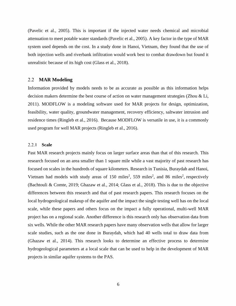
Figure 2-1 provides an estimation of the transmissivity of the entire Potomac Aquifer throughout
Virginia (Trapp Jr. & Horn, 1997). Based on the location of the site being modeled for this
research, the transmissivity value appears to be between 10,000 and 20,000 ft2/day.
9
Figure 2-1. Map of the Potomac Aquifer System displaying the estimated range of transmissivity
values (Trapp Jr. & Horn, 1997).
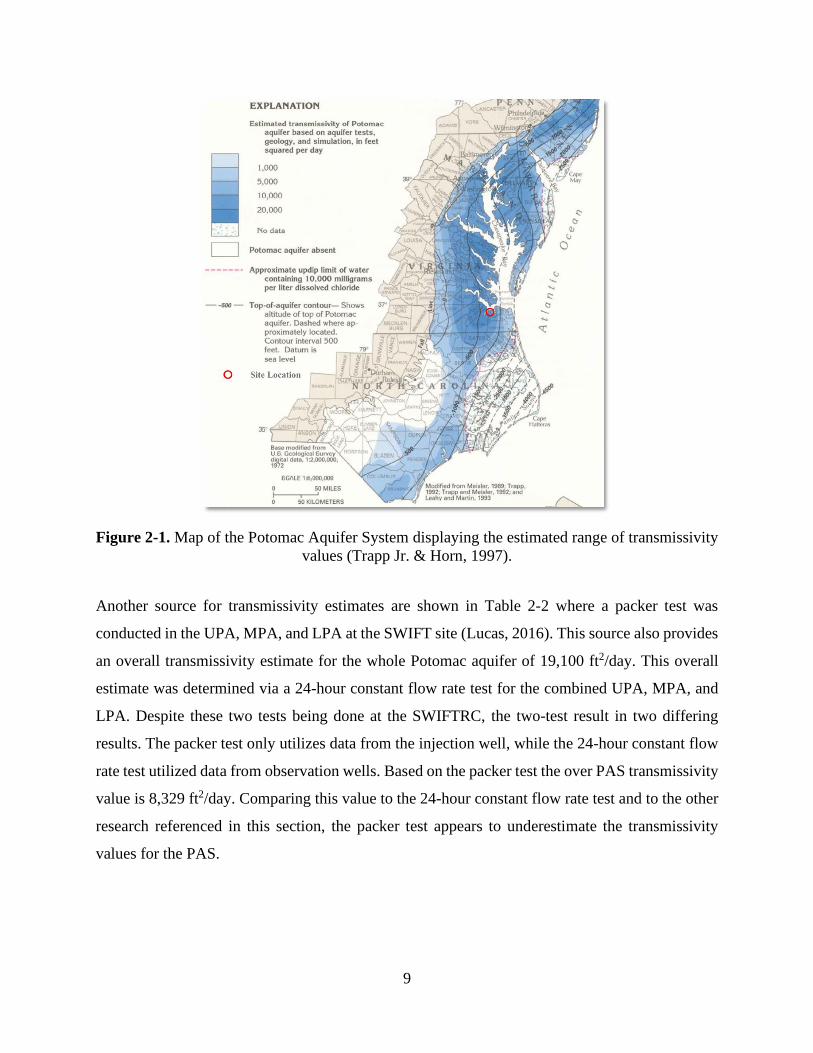
Another source for transmissivity estimates are shown in Table 2-2 where a packer test was
conducted in the UPA, MPA, and LPA at the SWIFT site (Lucas, 2016). This source also provides
an overall transmissivity estimate for the whole Potomac aquifer of 19,100 ft2/day. This overall
estimate was determined via a 24-hour constant flow rate test for the combined UPA, MPA, and
LPA. Despite these two tests being done at the SWIFTRC, the two-test result in two differing
results. The packer test only utilizes data from the injection well, while the 24-hour constant flow
rate test utilized data from observation wells. Based on the packer test the over PAS transmissivity
value is 8,329 ft2/day. Comparing this value to the 24-hour constant flow rate test and to the other
research referenced in this section, the packer test appears to underestimate the transmissivity
values for the PAS.
10
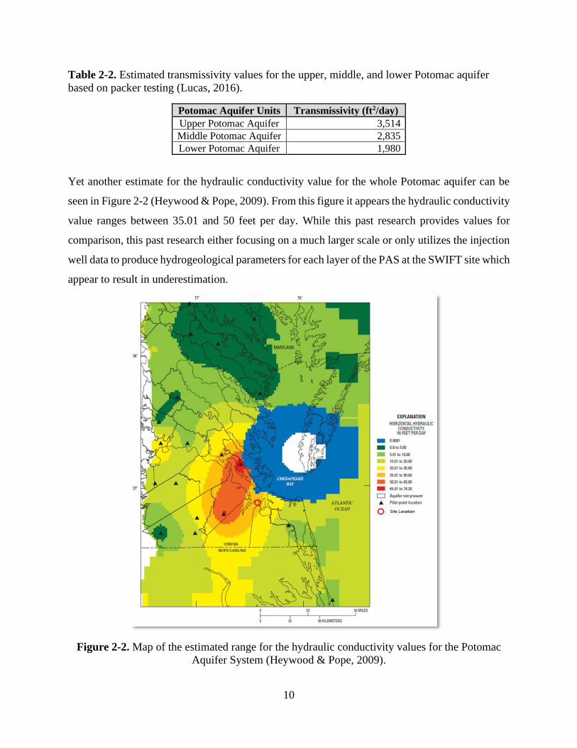
Table 2-2. Estimated transmissivity values for the upper, middle, and lower Potomac aquifer
based on packer testing (Lucas, 2016).
Potomac Aquifer Units Transmissivity (ft2/day)
Upper Potomac Aquifer 3,514
Middle Potomac Aquifer 2,835
Lower Potomac Aquifer 1,980
Yet another estimate for the hydraulic conductivity value for the whole Potomac aquifer can be
seen in Figure 2-2 (Heywood & Pope, 2009). From this figure it appears the hydraulic conductivity
value ranges between 35.01 and 50 feet per day. While this past research provides values for
comparison, this past research either focusing on a much larger scale or only utilizes the injection
well data to produce hydrogeological parameters for each layer of the PAS at the SWIFT site which
appear to result in underestimation.
Figure 2-2. Map of the estimated range for the hydraulic conductivity values for the Potomac
Aquifer System (Heywood & Pope, 2009).

11
It is important to note that due to stratification of the Coastal Plain sediments, the horizontal
hydraulic conductivity usually is greater than vertical hydraulic conductivity. This means that flow
through the confined aquifers is primarily in the lateral direction (McFarland & Bruce, 2006).
3 Data Sources
Wells
In total, data from eight wells were available for this investigation. Table 3-1 describes the wells
and information about each well. The location of each of these wells relative to the SWIFTRC can
be seen in Figure 1-3 above.
Table 3-1. Well data used for modeling in this study, such as Well I.D., well elevation, well
operator, data type and aquifer being monitored.
Well Screening
The wells at the SWIFT site are screened across the major permeable units of the UPA, MPA, and
LPA. Figure 3-1 shows a conceptual model of the PAS with the SWIFT MWs and a depiction of
Well I.D.
Elevation Above
Sea Level from
Land Surface (ft.)
Data
Source Data Type
Aquifer
Screened
Borehole
Log Data
TW-1 13.86 SWIFT
Flow Rate
and Water
Levels
UPA,
MPA, LPA Yes
MW-SAT 13.44 SWIFT Water
Quality
UPA,
MPA, LPA Yes
MW-UPA 11.45 SWIFT Water
Levels UPA Yes
MW-MPA 11.21 SWIFT Water
Levels MPA Yes
MW-LPA 10.79 SWIFT Water
Levels LPA Yes
USGS 59D 36 16.68 USGS Water
Levels UPA
One set of
data for all
three wells
USGS 59D 35 16.68 USGS Water
Levels MPA
USGS 59D 34 16.68 USGS Water
Levels LPA

12
the screens within each well (SWIFT & USGS, 2018). Test well (TW-1) is a multi-screen well
designed for a recharge at 700 gpm and for pumping at 1,400 gpm. Table 3-2 shows the length,
depth, and the hydrogeologic unit of the PAS of the 11 screens in TW-1. Three conventional
monitoring wells (UPA-MW, MPA MW, and LPA MW) are constructed with multiple screens in
the three hydrogeologic units of the PAS. Table 3-3, Table 3-4, and Table 3-5 shows the length,
depth and location of each of the screens in the three SWIFT conventional monitoring wells,
respectively. Although SAT-MW was instrumented with a pressure transducer at three of the
eleven sampling zones, water level data were evaluated and determined not to be viable for this
study as the water level data did not respond to the pumping test (see Figure A-1 and Figure A-2
in the Appendix).
Figure 3-1. Conceptual cross section model of the SWIFT wells depicting the aquifer layers, the
well depths, the screening for each well, and the distance each monitoring well is from TW-1 (SWIFT & USGS, 2018).

13
Table 3-2. TW-1 well screens including depths, lengths, and aquifer unit.
Screen I.D. Starting Depth (ft,bg) Ending Depth (ft,bg) Length (ft) Aquifer Unit
Screen 1 505 530 25 UPA
Screen 2 550 595 45 UPA
Screen 3 665 680 15 UPA
Screen 4 720 755 35 UPA
Screen 5 820 835 15 MPA
Screen 6 860 890 30 MPA
Screen 7 905 920 15 MPA
Screen 8 965 990 25 MPA
Screen 9 1050 1090 40 MPA
Screen 10 1230 1335 105 LPA
Screen 11 1370 1400 30 LPA
Table 3-3. SWIFT UPA monitoring well screen depths and lengths.
Screen
I.D. Starting Depth (ft.bg) Ending Depth (ft.bg)
Length
(ft)
Screen 1 515 565 50
Screen 2 585 605 20
Screen 3 660 675 15
Screen 4 710 740 30
Table 3-4. SWIFT MPA monitoring well screen depths and lengths.
Screen
I.D. Starting Depth (ft.bg) Ending Depth (ft.bg)
Length
(ft)
Screen 5 860 920 60
Screen 6 975 990 15
Screen 7 1030 1090 60
Table 3-5. SWIFT LPA monitoring well screen depths and lengths.
Screen
I.D. Starting Depth (ft.bg) Ending Depth (ft.bg)
Length
(ft)
Screen 8 1260 1320 60
Screen 9 1350 1410 60
Well Data Sets
Data at the SWIFTRC wells were recorded in one-minute intervals starting in May 2018. Data at
the three USGS wells were recorded in six-minute intervals starting in 2017 (USGS, n.d.). Depth
14
to water were recorded at both the SWIFT and USGS monitoring wells. Water level data for TW-
1 was not utilized as TW-1 is screened within all three aquifer layers and therefore cannot be used
to determine hydrogeological parameters for one of the three layers. It is also unknow what the
water level data from TW-1 represents, it could be the average head value of all three aquifer
layers, but this is unknown. Hydraulic head relative to sea level were determined as the difference
between land surface elevations and depth to water data.
For use in this research, two separate intervals of data were used for each well. These two separate
intervals of data acted at pump tests as the TW-1 pumps at a near constant rate. However,
performing a pump test for these two intervals of data was not intended goal of pumping. The first
interval of data used started August 3rd, 2018 at 9:32pm and ran for a duration of 1,440 min (1.0
day). This data set is referred to as the 8/18 data set. The second interval of data used started April
26th, 2019 at 9:29am and ran for a duration of 432 min (0.32 days). This data set is referred to as
the 4/19 data set. The two data sets were monitored and recorded immediately following time
periods in which TW-1 had not been in operation for at least 22 hours beforehand. After a review
of the water level data, this period of inactivity at TW-1 allowed water levels in the aquifer system
to return to a natural condition of steady state.
The data sets were positioned before and after TW-1 underwent rehabilitation. For the 9/18 data
set, TW-1 was pumping at an average of 1,109 GPM, with the removal rate being nearly constant
over the one-day time period. At the start of the 4/19 data set, TW-1 began to remove an average
of 683 GPM for the first five minutes, then the removal rate increased to 1,105 GPM with the
removal rate being nearly constant over the remainder of the 0.3-day time period.
The water level data recorded during these time intervals for the monitoring wells were used to
calculate hydrogeological parameters such as transmissivity and storage coefficients. These same
data sets were used in the modeling process. The data sets used for modeling can be seen in Table
A-8 and Table A-9. Data for the LPA is not provided as the LPA was not considered for this
research. In order to delineate both the low and high-resolution layer definitions for the aquifer
system, the borehole logs (see Appendix) for the swift site wells as well as the apparent
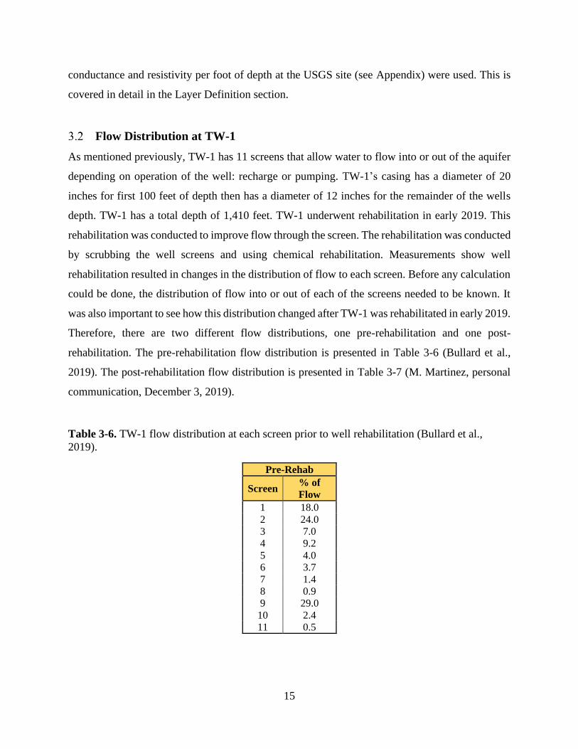
15
conductance and resistivity per foot of depth at the USGS site (see Appendix) were used. This is
covered in detail in the Layer Definition section.
Flow Distribution at TW-1
As mentioned previously, TW-1 has 11 screens that allow water to flow into or out of the aquifer
depending on operation of the well: recharge or pumping. TW-1’s casing has a diameter of 20
inches for first 100 feet of depth then has a diameter of 12 inches for the remainder of the wells
depth. TW-1 has a total depth of 1,410 feet. TW-1 underwent rehabilitation in early 2019. This
rehabilitation was conducted to improve flow through the screen. The rehabilitation was conducted
by scrubbing the well screens and using chemical rehabilitation. Measurements show well
rehabilitation resulted in changes in the distribution of flow to each screen. Before any calculation
could be done, the distribution of flow into or out of each of the screens needed to be known. It
was also important to see how this distribution changed after TW-1 was rehabilitated in early 2019.
Therefore, there are two different flow distributions, one pre-rehabilitation and one post-
rehabilitation. The pre-rehabilitation flow distribution is presented in Table 3-6 (Bullard et al.,
2019). The post-rehabilitation flow distribution is presented in Table 3-7 (M. Martinez, personal
communication, December 3, 2019).
Table 3-6. TW-1 flow distribution at each screen prior to well rehabilitation (Bullard et al.,
2019).
Pre-Rehab
Screen % of
Flow
1 18.0
2 24.0
3 7.0
4 9.2
5 4.0
6 3.7
7 1.4
8 0.9
9 29.0
10 2.4
11 0.5

16
Table 3-7. TW-1 flow distribution at each screen following to well rehabilitation (M. Martinez,
personal communication, December 3, 2019).
Post Rehab
Screen % of
Flow
1 18.8
2 45.5
3 2.1
4 7.2
5 6.0
6 2.8
7 9.5
8 2.0
9 11.1
10 1.1
11 0.0
With these flow distributions the percent of flow derived from each of the three aquifer units was
calculated. Table 3-8 and Table 3-9 show the percent of flow going out of the UPA and MPA
based on the pre-rehabilitation and post-rehabilitation flow distributions, respectively, based on
the time-average flow rates. As mentioned before, the first five minutes for the 4/19 data set has
an average flow rate different than the rest of the data set.
Table 3-8. Flow rates from each aquifer layer for both the 8/18 and 4/19 data sets using the pre-
rehabilitation flow distribution.
Pre-Rehabilitation Flow Rates
Flow Rates 8/3/18 4/26/19 First 5 min
Units Total UPA MPA Total UPA MPA Total UPA MPA
% of Flow 100 58 39 100 58 39 100 58 39
GPM -1,109 -646 -433 -1,105 -643 -431 -683 -397 -266
ft3/day -213,569 -124,297 -83,292 -212,763 -123,828 -82,978 -131,465 -76,513 -51,271
Table 3-9. Flow rates from each aquifer layer for both the 8/18 and 4/19 data sets using the post
rehabilitation flow distribution.
Post Rehabilitation Flow Rates Flow Rates 8/3/18 4/26/19 First 5 min
Units Total UPA MPA Total UPA MPA Total UPA MPA
% of Flow 100 74 31 100 74 31 100 74 31
GPM -1,109 -817 -347 -1,105 -814 -346 -683 -503 -214
ft3/day -213,569 -157,322 -66,849 -212,763 -156,729 -66,597 -131,465 -96,842 -41,150
17
Borehole Data for SWIFT Monitoring Wells
Borehole well logs for the SWIFT MW-UPA, MW-MPA, and MW-LPA, as well as for MW-SAT
and TW-1 can be seen in the Appendix as Figure A-5 through Figure A-9. Well data provided
includes the longitude and latitude of each well, along with the well datum, borehole depth and the
depth at which each well screen starts and ends. Each borehole log includes the sediment type for
every foot of depth down the borehole. The sediment types had many descriptions ranging from
hard clay/hard layers to sand. In order to create both the lower and higher resolution models, these
sediment types needed to be sorted into three groups, one being aquifer sediment, the second being
non-aquifer or confining sediment, and the third group is sediment that is defined based on the
location within the aquifer, as it is made up of both sand and clay. The three groups, and the
sediment types that fall into each group can be seen in Table A-1 in the Appendix. For the USGS
well site, the apparent conductance and resistivity per foot of depth was provided (K. McCoy,
personal communication, June 4, 2019).

18
4 Methods and Model Description
This section begins by defining the lithologic makeup under the SWIFTRC. Then the natural
gradient and direction of flow is determined for the PAS while TW-1 is not active. Flowing this,
the process of creating the conceptual models for both the low- and high-resolution (single and
multi-layered) model is described. This is followed by the varying model runs conducted using
both the low- and high-resolution models.
Layer Definition
Figure 4-1 depicts a conceptual model of the PAS beneath the SWIFTRC showing both the aquifer
layers and confining units that make up the UPA, MPA, and LPA. From the borehole logs and the
USGS apparent conductance and resistivity data, vertical maps of each of the wells around the
SWIFTRC could be produced for both the lower resolution and the higher resolution models.
Figure 4-1. Conceptual model of the PAS beneath the SWIFTRC showing both the aquifer and
confining layered that make up the UPA, MPA, and LPA
Figure 4-2. Soil type with depth at TW-1 with the screened intervals and hydrologic units (Lucas,
2016). shows the lithologic log of the SWIFT site based on the borehole log from the site (Lucas,

19
2016). Based on Figure 4-2. Soil type with depth at TW-1 with the screened intervals and
hydrologic units (Lucas, 2016)., the borehole logs and the three sediment groups discussed above,
the lower resolution (single layer) and higher resolution (multi-layered) vertical maps for each
SWIFT well were created. These vertical maps indicate where the UPA started and ended, as there
are distinct clay layers both above and below with almost all sand, aside for two clay/silty clay
layers, in between. These two clay layers within the UPA were used as confining units when
creating the higher resolution model. This resulted in three aquifer sublayers for the higher
resolution UPA model. The MPA was not as clear in where it began as there are many layers of
clay/clay with sand throughout, and the aquifer soil type was almost all sand and clay combined.
Based on the borehole log from TW-1, there are three clay layers throughout the MPA. However,
they are spaced close together (26 feet or closer) with one much thicker than the others. This thick
clay layer was used as a confining unit resulting in two aquifer sublayers, one above and below
the thick clay layer, for the higher resolution MPA model. The confining unit between the MPA
and the LPA was clearly defined by a large layer of hard clay. As previously discussed, the LPA
was not considered in this paper so is therefore not mapped in this process.
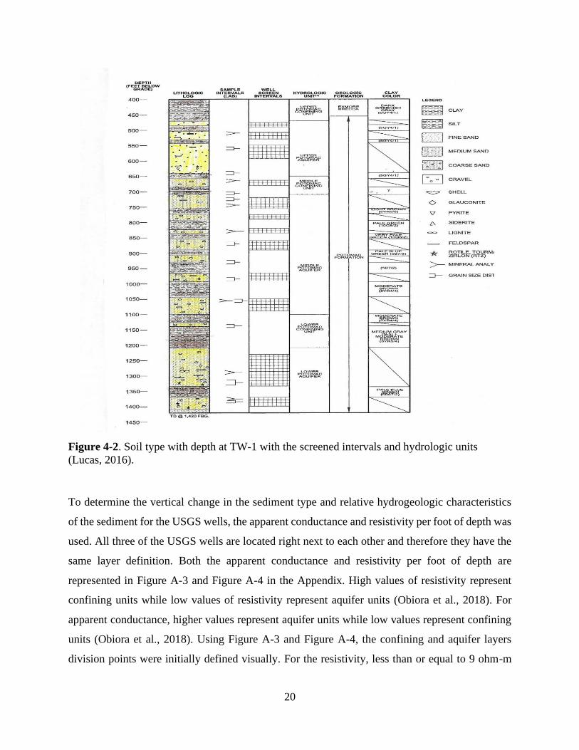
20
Figure 4-2. Soil type with depth at TW-1 with the screened intervals and hydrologic units
(Lucas, 2016).
To determine the vertical change in the sediment type and relative hydrogeologic characteristics
of the sediment for the USGS wells, the apparent conductance and resistivity per foot of depth was
used. All three of the USGS wells are located right next to each other and therefore they have the
same layer definition. Both the apparent conductance and resistivity per foot of depth are
represented in Figure A-3 and Figure A-4 in the Appendix. High values of resistivity represent
confining units while low values of resistivity represent aquifer units (Obiora et al., 2018). For
apparent conductance, higher values represent aquifer units while low values represent confining
units (Obiora et al., 2018). Using Figure A-3 and Figure A-4, the confining and aquifer layers
division points were initially defined visually. For the resistivity, less than or equal to 9 ohm-m
21
represented aquifer units and greater than 9 ohm-m represented confining units until a depth of
800 feet below ground level. After 800 feet below ground level the division point was changed,
for the resistivity, less than or equal to 6 ohm-m represented aquifer units and greater than 6 ohm-
m represented confining units. A similar process was done for the apparent conductance. For the
apparent conductance, less than or equal to 85 mmho/m represented confining units and greater
than 85 mmho/m represented aquifer units until a depth of 800 feet below the ground level. At 800
feet below ground level the division point was changed, for the apparent conductance, less than or
equal to 130 mmho/m represented confining units and greater than 130 mmho/m represented
aquifer units. The change at 800 feet below ground level is due to the apparent shift in the
sensitivity of the reading for both values. The cause of this shift is unknown; however, it could be
due to a change in equipment utilized or a shift in the reading as the equipment leaves the UPA
and enters the MPA. Table A-4 and Table A-5 provides the lithological mapping for all six
borehole locations for both the high resolution and the lower resolution models.
Figure 4-3 depicts the location of the cross sections seen in Figure 4-4 and Figure 4-5. Figure 4-4
and Figure 4-5 depict cross sections through GMS solids for both the UPA and MPA based on
both the higher and lower resolution lithological mapping previously discussed. Figure 4-5 depicts
the confining units with the UPA and MPA that are used to divide the aquifer layers into sublayers.
The method for creating GMS solids is discussed in detail later in this thesis.
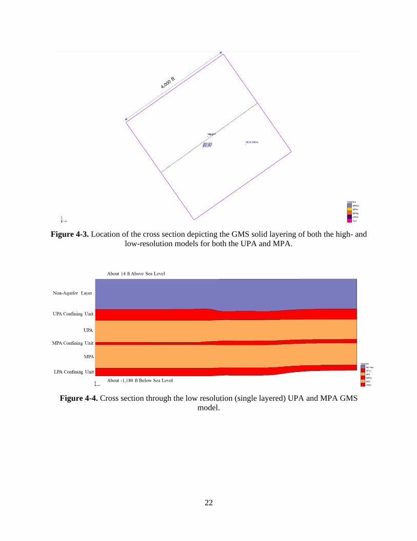
22
Figure 4-3. Location of the cross section depicting the GMS solid layering of both the high- and
low-resolution models for both the UPA and MPA.
Figure 4-4. Cross section through the low resolution (single layered) UPA and MPA GMS
model.
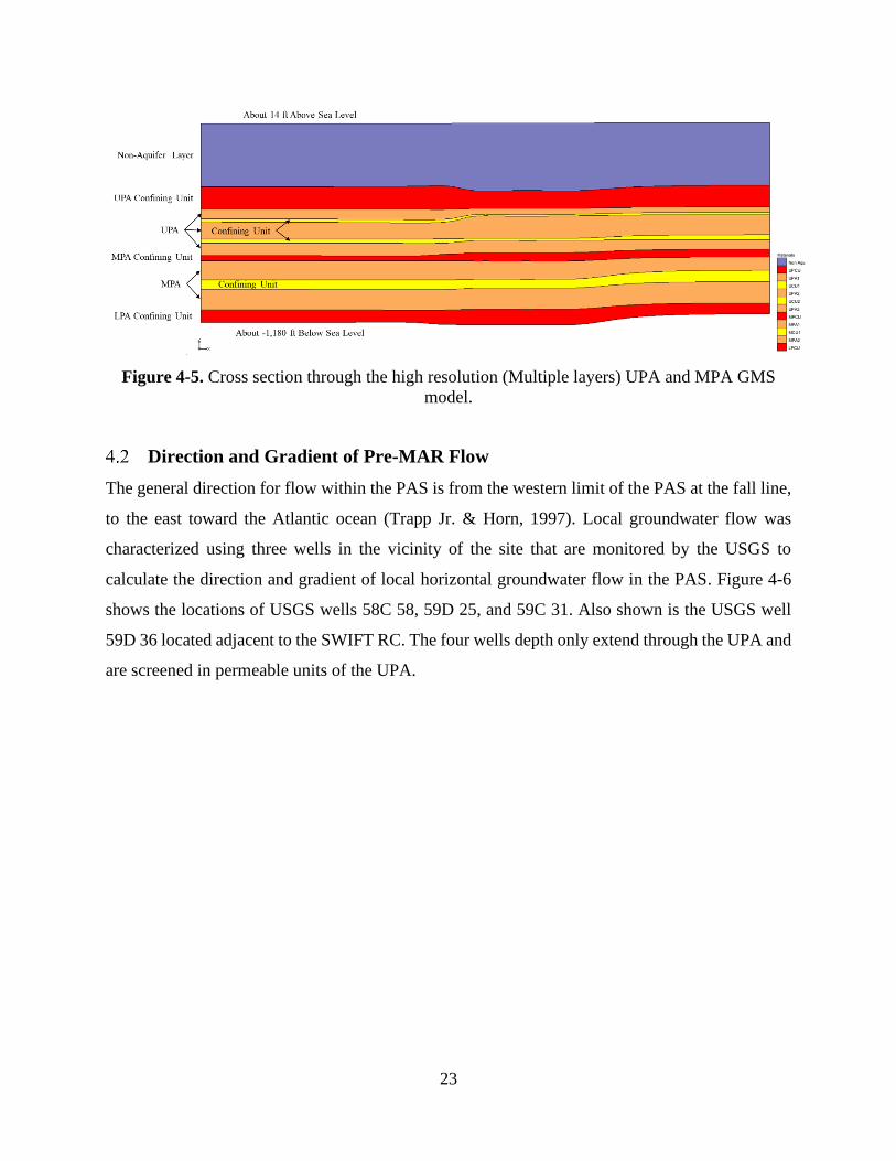
23
Figure 4-5. Cross section through the high resolution (Multiple layers) UPA and MPA GMS
model.
Direction and Gradient of Pre-MAR Flow
The general direction for flow within the PAS is from the western limit of the PAS at the fall line,
to the east toward the Atlantic ocean (Trapp Jr. & Horn, 1997). Local groundwater flow was
characterized using three wells in the vicinity of the site that are monitored by the USGS to
calculate the direction and gradient of local horizontal groundwater flow in the PAS. Figure 4-6
shows the locations of USGS wells 58C 58, 59D 25, and 59C 31. Also shown is the USGS well
59D 36 located adjacent to the SWIFT RC. The four wells depth only extend through the UPA and
are screened in permeable units of the UPA.
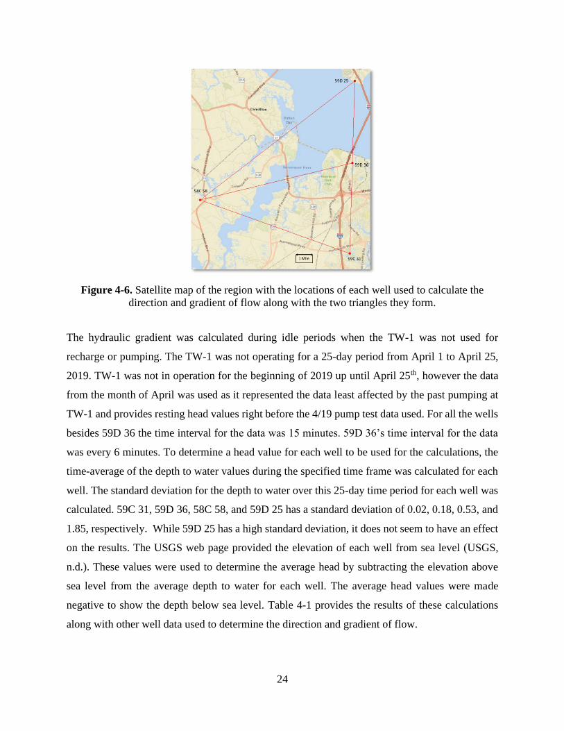
24
Figure 4-6. Satellite map of the region with the locations of each well used to calculate the
direction and gradient of flow along with the two triangles they form.
The hydraulic gradient was calculated during idle periods when the TW-1 was not used for
recharge or pumping. The TW-1 was not operating for a 25-day period from April 1 to April 25,
2019. TW-1 was not in operation for the beginning of 2019 up until April 25th, however the data
from the month of April was used as it represented the data least affected by the past pumping at
TW-1 and provides resting head values right before the 4/19 pump test data used. For all the wells
besides 59D 36 the time interval for the data was 15 minutes. 59D 36’s time interval for the data
was every 6 minutes. To determine a head value for each well to be used for the calculations, the
time-average of the depth to water values during the specified time frame was calculated for each
well. The standard deviation for the depth to water over this 25-day time period for each well was
calculated. 59C 31, 59D 36, 58C 58, and 59D 25 has a standard deviation of 0.02, 0.18, 0.53, and
1.85, respectively. While 59D 25 has a high standard deviation, it does not seem to have an effect
on the results. The USGS web page provided the elevation of each well from sea level (USGS,
n.d.). These values were used to determine the average head by subtracting the elevation above
sea level from the average depth to water for each well. The average head values were made
negative to show the depth below sea level. Table 4-1 provides the results of these calculations
along with other well data used to determine the direction and gradient of flow.
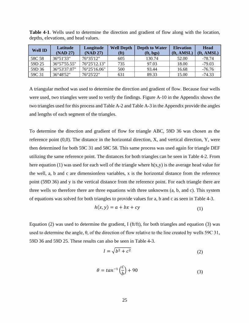
25
Table 4-1. Wells used to determine the direction and gradient of flow along with the location,
depths, elevations, and head values.
Well ID Latitude
(NAD 27)
Longitude
(NAD 27)
Well Depth
(ft)
Depth to Water
(ft, bgs)
Elevation
(ft, AMSL)
Head
(ft, AMSL)
58C 58 36°51'33" 76°35'12" 605 130.74 52.00 -78.74
59D 25 36°57'55.55" 76°25'12.13" 735 97.03 18.00 -79.03
59D 36 36°53'37.07" 76°25'16.06" 500 93.44 16.68 -76.76
59C 31 36°48'52" 76°25'22" 631 89.33 15.00 -74.33
A triangular method was used to determine the direction and gradient of flow. Because four wells
were used, two triangles were used to verify the findings. Figure A-10 in the Appendix shows the
two triangles used for this process and Table A-2 and Table A-3 in the Appendix provide the angles
and lengths of each segment of the triangles.
To determine the direction and gradient of flow for triangle ABC, 59D 36 was chosen as the
reference point (0,0). The distance in the horizontal direction, X, and vertical direction, Y, were
then determined for both 59C 31 and 58C 58. This same process was used again for triangle DEF
utilizing the same reference point. The distances for both triangles can be seen in Table 4-2. From
here equation (1) was used for each well of the triangle where h(x,y) is the average head value for
the well, a, b and c are dimensionless variables, x is the horizontal distance from the reference
point (59D 36) and y is the vertical distance from the reference point. For each triangle there are
three wells so therefore there are three equations with three unknowns (a, b, and c). This system
of equations was solved for both triangles to provide values for a, b and c as seen in Table 4-3.
ℎ(𝑥, 𝑦) = 𝑎 + 𝑏𝑥 + 𝑐𝑦 (1)
Equation (2) was used to determine the gradient, I (ft/ft), for both triangles and equation (3) was
used to determine the angle, θ, of the direction of flow relative to the line created by wells 59C 31,
59D 36 and 59D 25. These results can also be seen in Table 4-3.
𝐼 = √𝑏2 + 𝑐2 (2)
𝜃 = 𝑡𝑎𝑛−1 (𝑐
𝑏) + 90 (3)

26
Table 4-2. Distances in the X and Y direction from well 59D 36 for wells used to calculate
hydraulic gradient magnitude and direction.
Triangle ABC Triangle DEF
Wells X (ft) Y (ft) Wells X (ft) Y (ft)
59D 36 0 0 59D 36 0 0
59C 31 0 -28820 59D 25 0 26145
58C 58 -48184 -13200 58C 58 -48184 -13200
Table 4-3. Intermediate and final calculations for the hydraulic gradient magnitude (I) and
direction (𝜃) for both triangles.
Triangle ABC Triangle DEF
a1 -76.8 a2 -76.8
b1 -6.42E-05 b2 -6.49E-05
c1 8.43E-05 c2 8.68E-05
I1 (ft/ft) 1.06E-04 I2 (ft/ft) 1.08E-04
𝜃1 (deg) 37.28 𝜃2 (deg) 36.77
The average gradient between the two solutions is 0.000107 (ft/ft) and the average angle was
determined to be 37° counterclockwise from the reference line. The reference line created by wells
59C 31, 59D 36, and 59D 25 is less than one degree off a line that is perfectly north and south.
This result means the direction of flow is to the northwest. While the calculated flow direction is
different from the general flow pattern for the PAS, this result is consistent with the flow direction
reported for this region of the PAS (Trapp Jr. & Horn, 1997). This direction of flow could be
explained by the fact that the four largest permits for annual withdraw approved by Virginia are
all within Suffolk, King William or Isle of Wight county, which are all west/northwest of the
SWIFTRC (Virginia DEQ - Ground Water Withdrawal Permits and Fees, n.d.). These four permits
make up 49% of the total annual permitted withdraw within Virginia (Virginia DEQ - Ground
Water Withdrawal Permits and Fees, n.d.).
Hydrogeological Parameters
Using the 8/18 and 4/19 data sets and treating them as though where pumping test data sets,
transmissivity (T) and storage coefficients (S) for the UPA and the MPA were calculated. For
determining the UPA parameters, the UPA-MW and USGS-UPA wells data were analyzed. For
determining the MPA parameters, the MPA-MW and USGS-MPA wells data were used. The Theis
and the Cooper-Jacob methods were used to calculate the hydrogeological parameters (Schwartz
27
& Zhang, 2003) . To verify these methods could be utilized, the drawdown (s) versus time (t) was
plotted on a log-log scale for SWIFT-MW data sets (see Figure A-12, A-14, A-16, and A-18).
These plots were compared to diagnostics plots and determined to follow the Theis model, infinite
two-dimensional confined aquifer (Renard et al., 2009).
The Theis Type-Curve Method assumes that the aquifer is confined, homogeneous, isotropic, the
well is fully penetrating, the flow rate is constant, the flow is horizontal, head loss over the well
screen is negligible, and the confining units are non-leaky (Schwartz & Zhang, 2003). The Theis
method was implemented by plotting the drawdown (s) versus time (t) on a log-log scale,
overlaying this graph with the well function (W(u)) versus 1/u graph, and selecting a match point.
The corresponding W*(u) and s* values were used in the calculation of T, and 1/u* and t* values
were used in the calculation of S.
Equation (4) shows the Theis solution for calculation of drawdown (s(r,t)) based on the flow rate
(Q), the transmissivity (T) and the W(u).
𝑠∗(𝑟, 𝑡) =𝑄
4𝜋𝑇𝑊∗(𝑢) (4)
Rearranging equation (4) to solve for transmissivity results in equation (5).
𝑇 =
𝑄
4𝜋𝑠∗(𝑟, 𝑡)𝑊∗(𝑢) (5)
To solve for hydraulic conductivity equation (6) is used where K is hydraulic conductivity and b
is the aquifer vertical thickness.
𝐾 =
𝑇
𝑏 (6)
Equation (7) defines the dimensionless variable u. In equation (7), r is the radial distance from the
injection well, which in this case is radial distance from TW-1 to monitoring wells where
drawdown data are recorded, S is the storage coefficient. T is transmissivity, and t is time.
𝑢∗ =
𝑟2𝑆
4𝑇𝑡∗ (7)
28
To solve for the storage coefficient, equation (7) was rearranged resulting in equation (8).
𝑆 =
4𝑇𝑡∗𝑢∗
𝑟2 (8)
To solve for specific storage, equation (9) was used where Ss is the specific storage and b is the
aquifers vertical thickness.
𝑆𝑠 =
𝑆
𝑏 (9)
Figure 4-7 shows the overlay of 8/18 UPA-MW data set drawdown verses time graph with the
W(u) verses 1/u graph. As shown in Figure 4-7, the observation data at UPA-MW for 8/18 closely
follows the Theis curve. Figure A-12 through Figure A-19 in the Appendix show the data sets
used, the overlaid graphs and the Theis results for each data set and flow distribution. For the
differing flow distribution used of each data set, the only change in the calculations is using a new
Q value. Figure A-13, A-15, A-17, and A-19 show the USGS-MW data set drawdown verses time
graph with the W(u) verses 1/u graph. For all the USGS data sets besides the 4/19 USGS-MPA
data set, the drawdown verses time graph does not line up with the W(u) verses 1/u graph.

29
Figure 4-7. Drawdown vs time for the UPA-MW with the 8/18 data set overlayed on the W(u)
vs 1/u graph used for the Theis method.
For comparison, the Cooper-Jacob method was used on the same data sets as the Theis method
was used on. The Cooper-Jacobs method utilizes the same assumption as the Theis method. The
Cooper-Jacob method involves plotting the drawdown verses time with time being in log scale.
This should result in the data resembling a linear function. Figure 4-8 shows the 8/18 UPA-MW
data set drawdown verses time on a log scale.

30
Figure 4-8. Drawdown vs time on a log scale for the UPA-MW with the 8/18 data set used for
the Cooper-Jacob method.
Each data set was visually analyzed to determine the best-fit line following the early-time data.
The R2 values was used to help verify the fit of the semi-log line. Equation (10) represents the
best-fit equation based on the data points used from the 8/18 UPA-MW data set, where t is time
and s is the drawdown.
𝑠 = 0.8832 ln(𝑡) − 1.3014 (10)
To calculate the transmissivity, T, equation (11) was rearranged to equation (12) (Schwartz &
Zhang, 2003). Two points from the data set were then chosen. One point provided the first
drawdown value, s1, and the first time, t1. The second point provided the second drawdown value,
s2, and the second time, t2. Q represents the flow rate.
∆𝑠 = 𝑠2 − 𝑠1 =
2.303𝑄
4𝜋𝑇log
𝑡2𝑡1
(11)
𝑇 =
2.303𝑄
4𝜋∆𝑠log
𝑡2𝑡1
(12)
y = 0.8832ln(x) - 1.3014R² = 0.9996
0
1
2
3
4
5
6
0.1 1 10 100 1000 10000
Dra
wd
ow
n, s (
ft)
Time, t (min)
Cooper-Jacob Method with 8/18 data from the UPA-MW
31
Equation (6) was again used to calculate the hydraulic conductivity from the transmissivity values.
Before the storage coefficient could be calculated, the time when the straight line intersects the
line of zero drawdown (s=0) needed to be found, t0. This required rearranging equation (10) and
plugging zero in for drawdown as seen in equation (13).
𝑡0 = 𝑒
(0+1.3014)0.8832 (13)
With t0, the storage coefficient (S) is calculated using equation (14). Where r is the distance from
the injection well, which in this case is TW-1, to the monitoring wells from which the drawdown
data are used, which in this case is the UPA-MW. T represents the transmissivity.
𝑆 =
2.25𝑇𝑡0𝑟2
(14)
Equation (9) was used to calculate the specific storage from the storage coefficient values.
Figure A-12 through Figure A-19 in the Appendix shows the data set, graph drawdown vs time in
log scale, and the Cooper-Jacob method results for each data set and flow distribution. As noted
above for the Theis method, the differing flow distribution used for each data set requires updates
to Q in the calculation of T and S.
Like the Theis method, there were multiple instances where the USGS data cannot be used as the
data did not respond to the pumping in a way that hydrogeological parameters could be calculated.
For the Cooper-Jacob method the USGS-UPA 4/19 and the USGS-MPA 8/18 data sets did not
form a linear line that could be used for the Cooper-Jacob method (as seen in Figure A-15 and A-
17). The USGS-UPA 8/18 and USGS-MPA 4/19 data sets were usable with the Cooper-Jacob
method as a linear line of best fit could be created (as seen in Figure A-13 and Figure A-19).
GMS/MODFLOW
A conceptual model was created in the groundwater modeling system (GMS) as a precursor to
constructing a groundwater flow model using MODFLOW. Figure 4-9 depicts a conceptual model
of the whole PAS with each aquifer layer as a single GMS solid layer. GMS tutorials were
consulted to create conceptual models using GMS (GMS 10.4 Tutorials | Aquaveo.Com, n.d.). The

32
PEST package allows the user to employ parameter estimation based on observed data to estimate
hydrogeological parameters within the model domain (MODFLOW-Automated Parameter
Estimation, n.d.).
Figure 4-9. GMS model of the research site depicting the aquifer layers and the wells used.
Modeling Assumptions
Before modeling began multiple assumptions were made to simplify the modeling process or to fit
the requirements of the GMS application. The assumptions are listed below:
• Used general head boundaries, GHB, for the 4 vertical boundaries of the model. This is
because the head and flow rate are not known and cannot be assumed constant. However,
the head is assumed to be constant some distance away from the well where the pumping
does not affect the head and thus a GHB can be used. The use of GHB’s requires a
conductance value be entered into each of the four vertical boundaries. This conductance
value (same value for all four boundaries) was one of the three parameters to undergo
parameter estimation with PEST.

33
• Confining units are no flow boundaries as the hydraulic conductivity values are
significantly smaller than that of the aquifer layers and are assumed to not be leaking
confining units. This conforms to the Theis and Cooper-Jacob methods assumption and
diagnostic plot comparison (Renard et al., 2009).
• There is refinement of the grids cell size around TW-1 to better model the greater change
in head seen closer to TW-1.
• Each aquifer layer is homogeneous and isotropic.
• The borehole log for the UPA does not record soil type data past the depth of the UPA.
Therefore, the gap in data for the MPA from the UPA log is assumed to be the same found
in the MPA borehole log.
• The effective porosity for each aquifer layer is equal to the porosity of each layer. 0.27 for
the UPA and 0.28 for the MPA (Bullard et al., 2019).
• Only considering horizontal hydraulic conductivity, as the vertical is assumed to be much
less than the horizontal.
GMS Base Models
The domain of the groundwater models created for this research was centered around the TW-1
with equal horizontal dimensions of 4,000 ft. by 4,000 ft. or 0.594 square miles and is oriented
with the direction of natural groundwater flow as seen in Figure 4-10. The domain size was chosen
because it encompasses all the MWs being used. The domain is big enough to visualize the cone
of depression and encompass any new wells that may be drilled around the site. Because of the
number of wells and their limited spacing from each other, bigger domains resulted in lower
confidence in the lithologic makeup, which resulted in keeping the domain smaller in scale. The
grid size was set to 20 ft with refinement around TW-1 with a minimum size of 10 ft. This grid
size was chosen as it is small enough to provide a high resolution of detail while not too small to
result in slow model times. There was refinement around TW-1 because there is a greater change
in head around TW-1 and this refinement will help properly model this larger change in head. The
model depths varied depending on which of the two confined aquifers (UPA or MPA) was being
modeled.
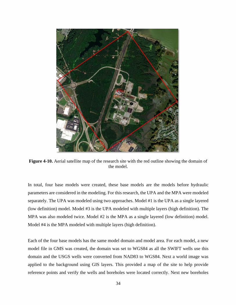
34
Figure 4-10. Aerial satellite map of the research site with the red outline showing the domain of
the model.
In total, four base models were created, these base models are the models before hydraulic
parameters are considered in the modeling. For this research, the UPA and the MPA were modeled
separately. The UPA was modeled using two approaches. Model #1 is the UPA as a single layered
(low definition) model. Model #3 is the UPA modeled with multiple layers (high definition). The
MPA was also modeled twice. Model #2 is the MPA as a single layered (low definition) model.
Model #4 is the MPA modeled with multiple layers (high definition).
Each of the four base models has the same model domain and model area. For each model, a new
model file in GMS was created, the domain was set to WGS84 as all the SWIFT wells use this
domain and the USGS wells were converted from NAD83 to WGS84. Next a world image was
applied to the background using GIS layers. This provided a map of the site to help provide
reference points and verify the wells and boreholes were located correctly. Next new boreholes

35
were created and located in their correct positions based on their longitude and latitude. Next a
new coverage was created, and the outline of the model boundary was drawn with each side of the
square being 4,000 feet long. This outline was then centered on TW-1 and rotated 37°
counterclockwise from the vertical or 53° clockwise from the horizontal. From here the vertices
were redistributed along the outline so that they were evenly spaced 40 ft apart. Next a polygon
was built from the outline and this was mapped to a new TIN which can be seen in Figure 4-11.
Figure 4-11. Model domain with the location of TW-1 and the TIN mesh.
From here the single layer and multi-layered models differ as the layer definitions that were entered
into each of the boreholes were different. For the single layered models, the starting depth of each
layer of the UPA and MPA can be seen in Table A-4. For the multi-layered models, the starting
depth of each layer of the UPA and MPA can be seen in Table A-5. Both tables also provide the
horizon labels for each layer used. These horizons are needed to build GMS solids from the
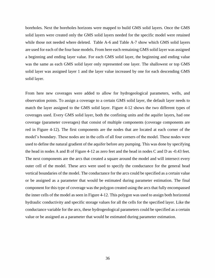
36
boreholes. Next the boreholes horizons were mapped to build GMS solid layers. Once the GMS
solid layers were created only the GMS solid layers needed for the specific model were retained
while those not needed where deleted. Table A-6 and Table A-7 show which GMS solid layers
are used for each of the four base models. From here each remaining GMS solid layer was assigned
a beginning and ending layer value. For each GMS solid layer, the beginning and ending value
was the same as each GMS solid layer only represented one layer. The shallowest or top GMS
solid layer was assigned layer 1 and the layer value increased by one for each descending GMS
solid layer.
From here new coverages were added to allow for hydrogeological parameters, wells, and
observation points. To assign a coverage to a certain GMS solid layer, the default layer needs to
match the layer assigned to the GMS solid layer. Figure 4-12 shows the two different types of
coverages used. Every GMS solid layer, both the confining units and the aquifer layers, had one
coverage (parameter coverages) that consist of multiple components (coverage components are
red in Figure 4-12). The first components are the nodes that are located at each corner of the
model’s boundary. These nodes are in the cells of all four corners of the model. These nodes were
used to define the natural gradient of the aquifer before any pumping. This was done by specifying
the head in nodes A and B of Figure 4-12 as zero feet and the head in nodes C and D as -0.43 feet.
The next components are the arcs that created a square around the model and will intersect every
outer cell of the model. These arcs were used to specify the conductance for the general head
vertical boundaries of the model. The conductance for the arcs could be specified as a certain value
or be assigned as a parameter that would be estimated during parameter estimation. The final
component for this type of coverage was the polygon created using the arcs that fully encompassed
the inner cells of the model as seen in Figure 4-12. This polygon was used to assign both horizontal
hydraulic conductivity and specific storage values for all the cells for the specified layer. Like the
conductance variable for the arcs, these hydrogeological parameters could be specified as a certain
value or be assigned as a parameter that would be estimated during parameter estimation.
37
Figure 4-12. Depiction of the two coverage types with the red showing the nodes, arcs, and
polygons used to specify hydrogeological parameters. Blue shows the wells used for observation
data, refinement, and pumping flow rates.
The confining unit GMS solid layers only have parameter coverage layers as they do not have any
of the wells screened in them for flow or observation data. However, the aquifer unit GMS solid
layers have wells screened in them for flow or observation data and there for a second type of
coverage (well coverages) are required for these layers. The components for this type of coverage
can also be seen in Figure 4-12 as the blue components. TW-1 needed to be added to each layer as
a well that had a screen the length of the sum of the screen lengths in the GMS solid aquifer layer.
The screen needed to have a starting and ending depth that was within the depth of the aquifer
layer. This well was also used to specify the cell size of the grid and had refinement around the
well. The cells had a max size of 20 ft with a refinement of 10 ft around TW-1. The second
Red - Parameter Coverage
Blue - Well Coverage
38
component of these coverage types was the observation points. Every coverage had a point at the
USGS well location regardless of if the UPA or the MPA was being modeled. However, the UPA-
MW was only used for UPA models and the MPA-MW was only used for MPA models. The type
of observation data used within MODFLOW depended on if the model was a transient or steady
state model.
The next step was to create a new grid frame. This grid frame perfectly outlined the arcs of the
parameter coverages which means each side of the frame is 4,000 feet long, was centered around
TW-1, and has the necessary rotation. This grid frame was used to create a 3D finite difference
grid and used refinement points. The X and Y dimensions were specified by the grid frame. The Z
dimension had the number of cells equal to the number of GMS solid unit layers. The origin for
the Z dimension was set to -1500 feet and the length was set to 1600 feet. These values were chosen
because this would result on an initial grid that fully encompasses the GMS solid layers.
Next a new MODFLOW model was created to allow for the GMS solids to be mapped to the
MODFLOW model/grid. To map the GMS solids to the model/grid, boundary matching was used.
The resulting MODFLOW models /grids sizing for each of the base models can be seen in Figure
4-13.

39
Figure 4-13. Depiction of model grid centered and refined around TW-1. Zoomed in to better
show cell sizing.
Every model used MODFLOW 2005 and had starting head values of zero for every layer. For
parameter estimation models, three packages were used. GHB1-General Head Boundary, PEST-
ASP and WEL1-Well are the three packages used. GHB1 was used to define the vertical boundary
conditions of the model as GHB’s as discussed in the assumptions. PEST was used to allow for
parameter estimation of hydraulic conductivity, specific storage, and the conductance of the
GHB’s. WEL1 was used to allow for the use of wells in the model to model the addition or removal
of water from the aquifer through the screened portions of a well. For forward models, the PEST-
ASP package is not used as there is no parameter estimation. For steady state models the
observation data selected for coverages needed to be head only. For transient models, the
observation data selected for coverages needed to be transient head.

40
Single Layer Models and Parameter Estimation
Once the four base models were created, the MODFLOW models were executed to determine
hydrogeological parameters and simulate head values. MODPATH was used to calculate travel
times. Table 4-4 describes how base single layered Models 1 and 2 were used for different model
runs with varying combinations of flow distributions, data sets, model types, run options and
weighting to determine hydrogeological parameters.
Model runs were conducted to determine the optimal hydrogeological parameters that best
simulate observations data sets. The initial hydrogeological parameter values entered into each of
the transient runs for both Models 1 and 2 were based on the average between the Theis and
Cooper-Jacob calculations. For the transient models, the time steps and multipliers needed to be
specified. To determine these values, Model-run 1-1 was conducted multiple times with varying
values for both the number of time steps and multipliers to find the combination that resulted in
the lowest model error. The model error represents the deviation of the best possible estimate for
the change in head compared to the true observed value. The magnitude of the model error value
for each run of model-run 1-1 was affected by the weighting/standard deviation of the observation
data, however, the percent change in the model error from one run to another did not change. This
means that regardless of the weigh value for the observation points, the same combination for the
number of time steps and multiplier result in the lowest model error. Table 4-5 displays the model
error for each run of Model-run 1-1 with multiple combinations of the number of time steps and
multipliers. For each run the weight for both the USGS and SWIFT MWs was set to one. From
this table, 60-time steps and a multiplier of 1.2 was chosen for all the transient models. These
values were chosen because the error did not decrease as more time steps were added, and the
more time steps used the longer the model run times. A maximum value allowed for the multiplier
was 1.2 as it is recommended by the USGS not to exceed 1.2 (ModelMuse Help: Time Step
Options, n.d.). For every transient model, the first stress period had a length of zero, one-time step,
a multiplier of 1 and was steady state. This was done to determine the initial head values before
any pumping and was based on the natural gradient of the groundwater. This meant that TW-1 had
a pumping flow rate of zero for the first stress period. For model runs using the 8/18 data set, the
second stress period started at zero and had a length of one day. For model runs using the 4/19 data
set, the second stress period has a length of 5 minutes or 0.00347 days to accommodate for the

41
different removal rate for the first 5 minutes of pumping. There are five time steps and a multiplier
of 1 for this second stress period. The third stress period starts at 0.00347 days and ends at 0.3
days.
Table 4-4. Model runs implemented to determine hydrogeological parameters utilizing
parameter estimation, while forward model runs compared results using hydrogeological
parameters from 8/18 model runs to 4/19 data sets.
Model #
-Run # °
Data
Set
Flow
Rate+
Flow Rate
Distribution Run Option
USGS Ob.
Point
Weighting
SWIFT MW
Ob. Point
Weighting
Starting
hydrogeological
parameters values*
1-1 8/18 8/18 Pre Parameter Est. 1 1 Calculated
1-2 8/18 8/18 Pre Parameter Est. 1 4 Below Calculated
1-2 8/18 8/18 Pre Parameter Est. 1 4 Above Calculated
1-3 8/18 8/18 Pre Parameter Est. NA 1 Calculated
1-4 8/18 8/18 Post Parameter Est. 1 1 Calculated
1-5 8/18 8/18 Post Parameter Est. 1 4 Below Calculated
1-5 8/18 8/18 Post Parameter Est. 1 4 Above Calculated
1-6 8/18 8/18 Post Parameter Est. NA 1 Calculated
1-7 4/19 4/19 Pre Forward NA NA From 1-2
1-8 4/19 4/19 Pre Parameter Est. 1 1 Calculated
1-9 4/19 4/19 Pre Parameter Est. 1 4 Below Calculated
1-9 4/19 4/19 Pre Parameter Est. 1 4 Above Calculated
1-10 4/19 4/19 Pre Parameter Est. NA 1 Calculated
1-11 4/19 4/19 Post Forward NA NA From 1-5
1-12 4/19 4/19 Post Parameter Est. 1 1 Calculated
1-13 4/19 4/19 Post Parameter Est. 1 4 Below Calculated
1-13 4/19 4/19 Post Parameter Est. 1 4 Above Calculated
1-14 4/19 4/19 Post Parameter Est. NA 1 Calculated
2-1 8/18 8/18 Pre Parameter Est. 1 1 Calculated
2-2 8/18 8/18 Pre Parameter Est. 1 4 Below Calculated
2-2 8/18 8/18 Pre Parameter Est. 1 4 Above Calculated
2-3 8/18 8/18 Pre Parameter Est. NA 1 Calculated
2-4 8/18 8/18 Post Parameter Est. 1 1 Calculated
2-5 8/18 8/18 Post Parameter Est. 1 4 Below Calculated
2-5 8/18 8/18 Post Parameter Est. 1 4 Above Calculated
2-6 8/18 8/18 Post Parameter Est. NA 1 Calculated
2-7 4/19 4/19 Pre Forward NA NA From 2-2
2-8 4/19 4/19 Pre Parameter Est. 1 1 Calculated
2-9 4/19 4/19 Pre Parameter Est. 1 4 Below Calculated
2-9 4/19 4/19 Pre Parameter Est. 1 4 Above Calculated
2-10 4/19 4/19 Pre Parameter Est. NA 1 Calculated
2-11 4/19 4/19 Post Forward NA NA From 2-5
2-12 4/19 4/19 Post Parameter Est. 1 1 Calculated
2-13 4/19 4/19 Post Parameter Est. 1 4 Below Calculated
2-13 4/19 4/19 Post Parameter Est. 1 4 Above Calculated
2-14 4/19 4/19 Post Parameter Est. NA 1 Calculated
° Model # 1 represents UPA single layer model, Model # 2 represents MPA single layer model.
+ Flow Rates values are the calculated average over the time period.
* Starting estimated hydrogeological parameters values based on averages of Theis and Cooper-Jacob results.

42
Table 4-5. Model iterations to determine the optimal multiplier and the optimal number of time
steps.
8/18 Data and Pre-Flow
Number of
Time Steps Multiplier Model Error
20 1.2 6.98
40 1.1 6.86
60 1.1 6.78
80 1.1 6.77
100 1.1 6.77
120 1.1 6.77
140 1.1 6.77
40 1.2 6.77
60 1.2 6.76
80 1.2 6.76
100 1.2 6.76
The removal rates from TW-1 and observation data needed to be added to the well coverages for
the aquifer layer. For the UPA observation points, the UPA had two points each within the aquifer
layer of the model. One point was located at the USGS well site and the other was at the UPA-
MW site. The data that was entered into each point depended on if the 8/18 or the 4/19 data set
was being used. The data used for these two points for both data sets can be seen in Table A-8 in
the Appendix. For the MPA observation points, the MPA had two points each within the aquifer
layer of the model. One point was located at the USGS well site and the other was at the MPA-
MW site. The data used for these two points for both data sets can be seen in Table A-9 in the
Appendix.
For the flow rates of TW-1, the values used depended on the data set used and whether pre or post
rehabilitation flow distribution was being used. For both data sets the flow rate was set to transient
to allow for the flow rate to change with time. For the 8/18 data set the flow rates used for TW-1
can be seen in Table 4-6 where the negative means removal. For the 4/19 data set the flow rates
used for TW-1 can be seen in Table 4-7.

43
Table 4-6. TW-1 flow rates used to simulate the 8/18 data set for the UPA and MPA.
UPA Flow Rate (ft3/d) MPA Flow Rate (ft3/d)
Time (days) Per Rehab. Post Rehab. Per Rehab. Post Rehab.
0 0 0 0 0
0 -124,297 -157,322 -83,292 -66,849
1 -124,297 -157,322 -83,292 -66,849
Table 4-7. TW-1 flow rates used to simulate the 4/19 data set for the UPA and MPA.
UPA Flow Rate (ft3/d) MPA Flow Rate (ft3/d)
Time (days) Per Rehab. Post Rehab. Per Rehab. Post Rehab.
0 0 0 0 0
0 -76,513 -96,842 -51,271 -41,150
0.00347 -76,513 -96,842 -51,271 -41,150
0.00347 -123,828 -156,729 -82,978 -66,597
0.3 -123,828 -156,729 -82,978 -66,597
The observation data were weighted with the use of equation (15) where SD is the standard
deviation and GPW is the group weight. GPW was set to one for all of the observation points as
they are all within the same group, observation wells.
𝑊𝑒𝑖𝑔ℎ𝑡 =
1
(𝑆𝐷)2 ∗ 𝐺𝑃𝑊 (15)
Because the GPW was always one, the only way to change the weighting of a certain observation
point was by changing the SD value. Because most of the USGS monitoring wells data did not fit
the Theis curve and appeared corrupt, multiple weighting combinations were applied to multiple
model runs for base Models 1 and 2. These weighting combinations can be seen in Table 4-4. The
first combination has the SWIFT and USGS MW observation data weighed the same. The second
combination has the SWIFT MW observation data weighted 4 times greater than that of the USGS
MW observation data. The last combination only uses the SWIFT MW observation data and does
not consider the USGS MW observation data.
To test the uniqueness of the results for the transient/parameter estimation models, the model runs
for both base Models 1 and 2 that weighed the SWIFT MW observation data 4 times greater than
that of the USGS MW were conducted twice as seen in Table 4-4. These runs were conducted
twice, once where the initial hydrogeological parameter values were set to well below the average

44
between the Theis and Cooper-Jacob calculated results. The second was where the initial
hydrogeological parameter values were set to well above the average between the Theis and
Cooper-Jacob calculated results. The sensitivity of each parameter being estimated was analyzed,
using the same model-runs used for the uniqueness testing, to determine the effect each parameter
had on the model. This was done through MODFLOW with the PEST package.
The forward model runs were conducted to see how the results using the estimated hydrogeological
parameters from the 8/18 model runs would compare to the 4/19 observation data. Forward model
runs 1-7 and 1-11 focus on the UPA while forward model runs 2-7 and 2-11 focus on the MPA.
Models 1-7 and 2-7 used the estimated hydrogeological parameters from Models 1-2 and 2-2 (8/18
data set and pre-rehabilitation flow), respectively, and ran a forward model using the pre-
rehabilitation flow distribution. These model-run results were compared to the observed data from
the 4/19 data set. Model runs 1-11 and 2-11 used the estimated hydrogeological parameters from
Models 1-5 and 2-5 (8/18 data set and post rehabilitation flow), respectively, and ran a forward
model using the post rehabilitation flow distribution. These modeled results were compared with
the observed data from the 4/19 data set.
Multi-Layered Aquifer Models
In order to estimate drawdown and travel times for each sublayer of the UPA and MPA, the UPA
and the MPA needed to be divided into multiple sublayers. The depths at which each aquifer is
divided up into separate sublayers has already been discussed above. For the UPA, the aquifer was
divided into three aquifer sublayers (UPA L1, UPA L2, and UPA L3) separated by confining units
as seen in Figure 4-14. All the results for Models 1 and 2 can be seen in Table 5-5 in the results.

45
Figure 4-14. 3D depiction of the UPA domain with the aquifer divided into multiple sublayers.
While the MPA was divided into two aquifer sublayers (MPA L1 and MPA L2) separated by
confining units as seen in Figure 4-15.
Figure 4-15. 3D depiction of the MPA domain with the aquifer divided into multiple sublayers.

46
The hydrogeological parameters for each of these sublayers needed to be estimated. However, as
there is no observation data for every screen for each MW, it was not possible to perform parameter
estimation in GMS to estimate these hydrogeological parameter values for each sublayer.
Therefore, the hydrogeological parameters estimated from single-layered Models 1 and 2 were
used. From Models 1 and 2, the results from runs 3, 6, 10, and 14, which only used the SWIFT
MW observation data (Table 4-8), were used to calculate the hydrogeological parameters for each
sublayer of the multi-layered aquifers.
Table 4-8. Estimated transmissivity and specific storage values from Models 1 and 2 based on the
SWIFT monitoring wells observation data only.
Transmissivity (ft2/day) Specific Storage (1/ft)
8/18 4/19 8/18
4/19
Layer Q pre-
rehab.
Q post
rehab.
Q pre-
rehab.
Q post
rehab.
Q pre-
rehab.
Q post
rehab.
Q pre-
rehab.
Q post
rehab.
UPA 11,022 13,966 15,166 19,265 2.8E-06 3.5E-06 2.7E-06 3.4E-06
MPA 14,982 12,027 13,485 10,824 5.4E-06 4.4E-06 3.9E-06 3.1E-06
The first step to calculating the hydrogeological parameters for each of the sublayers for both the
UPA and MPA was to determine the distribution of flow for each sublayer. This was done by
determining which screens were in each sublayer and adding up the percent of flow distribution in
each screen within that sublayer. Table 4-9 provides a summary of which screens are in which
sublayer.
Table 4-9. Aquifer sublayer location of TW-1 screens.
Screen Sublayer
1 UPA L1
2 UPA L2
3 UPA L2
4 UPA L3
5 MPA L1
6 MPA L1
7 MPA L1
8 MPA L2
9 MPA L2
Using the flow values for each aquifer layer in Table 4-10 (from Table 3-8 and Table 3-9), and the
percent of total flow entering each sublayer, the flow entering each sublayer was calculated for

47
both data sets and both pre and post rehabilitation flow distributions. This was done by multiplying
the percent of total flow into each sublayer by the aquifer layer flow rate (Table 4-11).
Table 4-10. Pre and post rehabilitation flow distributions for both the UPA and the MPA for
both the 8/18 and 4/19 data sets.
% of Total Flow Flow for 8/18 (ft3/day) Flow for 4/19 (ft3/day)
Layer r(ft) Length
(ft)
Q pre-
rehab.
Q post
rehab.
Q pre-
rehab.
Q post
rehab.
Q pre-
rehab.
Q post
rehab.
UPA 340 240 58 74 -124,297 -157,322 -123,828 -156,729
MPA 390 231 39 31 -83,292 -66,849 -82,978 -66,597
Table 4-11. Pre and post rehabilitation flow rate data for both the 8/18 and 4/19 data sets for
each sublayer of the multi-layered models.
% of Total Flow Flow for 8/18 (ft3/day) Flow for 4/19 (ft3/day)
Sublayer Length
(ft)
Q pre-
rehab.
Q post
rehab.
Q pre-
rehab.
Q post
rehab.
Q pre-
rehab.
Q post
rehab.
UPA L1 33 18 19 -38,442 -40,060 -38,297 -39,909
UPA L2 134 31 48 -66,206 -101,793 -65,957 -101,409
UPA L3 73 9 7 -19,648 -15,469 -19,574 -15,410
MPA L1 107 9 18 -19,435 -38,983 -19,361 -38,836
MPA L2 124 30 13 -63,857 -27,866 -63,616 -27,761
To calculate the transmissivity and hydraulic conductivity values for each sublayer, the
transmissivity values from Table 4-8 were used. These model runs were chosen as they were the
models that only used the SWIFT monitoring wells for parameter estimation and not the USGS
wells. The USGS monitoring well data was not used, as much of the data appeared nonresponsive
to pumping or appeared noisy and/or corrupt. The model runs from which the results were used
depended on which data set, flow rate, and flow distribution was being used. To calculate the
transmissivity in each sublayer, Ti, equation (16) was used where TAtot is the transmissivity of the
whole aquifer layer (UPA or MPA). Qi is the flow rate for the sublayer and QAtot is the total flow
rate for the whole aquifer layer (UPA or MPA).
𝑇𝑖 = 𝑇𝐴𝑡𝑜𝑡 ∗ (
𝑄𝑖
𝑄𝐴𝑡𝑜𝑡) (16)
The hydraulic conductivity was calculated by taking the transmissivity for each sublayer and
dividing it by the length of that sublayer. Table 4-12. Calculated transmissivity and hydraulic
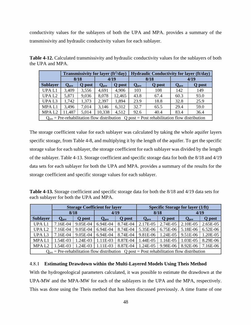
48
conductivity values for the sublayers of both the UPA and MPA. provides a summary of the
transmissivity and hydraulic conductivity values for each sublayer.
Table 4-12. Calculated transmissivity and hydraulic conductivity values for the sublayers of both
the UPA and MPA.
Transmissivity for layer (ft2/day) Hydraulic Conductivity for layer (ft/day)
8/18 4/19 8/18 4/19 Sublayer Qpre Q post Qpre Q post Qpre Q post Qpre Q post
UPA L1 3,409 3,556 4,691 4,906 103 108 142 149
UPA L2 5,871 9,036 8,078 12,465 43.8 67.4 60.3 93.0
UPA L3 1,742 1,373 2,397 1,894 23.9 18.8 32.8 25.9
MPA L1 3,496 7,014 3,146 6,312 32.7 65.5 29.4 59.0
MPA L2 11,487 5,014 10,338 4,512 92.6 40.4 83.4 36.4
Qpre = Pre-rehabilitation flow distribution Q post = Post rehabilitation flow distribution
The storage coefficient value for each sublayer was calculated by taking the whole aquifer layers
specific storage, from Table 4-8, and multiplying it by the length of the aquifer. To get the specific
storage value for each sublayer, the storage coefficient for each sublayer was divided by the length
of the sublayer. Table 4-13. Storage coefficient and specific storage data for both the 8/18 and 4/19
data sets for each sublayer for both the UPA and MPA. provides a summary of the results for the
storage coefficient and specific storage values for each sublayer.
Table 4-13. Storage coefficient and specific storage data for both the 8/18 and 4/19 data sets for
each sublayer for both the UPA and MPA.
Storage Coefficient for layer Specific Storage for layer (1/ft)
8/18 4/19 8/18 4/19
Sublayer Qpre Q post Qpre Q post Qpre Q post Qpre Q post
UPA L1 7.16E-04 9.05E-04 6.94E-04 8.74E-04 2.17E-05 2.74E-05 2.10E-05 2.65E-05
UPA L2 7.16E-04 9.05E-04 6.94E-04 8.74E-04 5.35E-06 6.75E-06 5.18E-06 6.52E-06
UPA L3 7.16E-04 9.05E-04 6.94E-04 8.74E-04 9.81E-06 1.24E-05 9.51E-06 1.20E-05
MPA L1 1.54E-03 1.24E-03 1.11E-03 8.87E-04 1.44E-05 1.16E-05 1.03E-05 8.29E-06
MPA L2 1.54E-03 1.24E-03 1.11E-03 8.87E-04 1.24E-05 9.98E-06 8.92E-06 7.16E-06
Qpre = Pre-rehabilitation flow distribution Q post = Post rehabilitation flow distribution
Estimating Drawdown within the Multi-Layered Models Using Theis Method
With the hydrogeological parameters calculated, it was possible to estimate the drawdown at the
UPA-MW and the MPA-MW for each of the sublayers in the UPA and the MPA, respectively.
This was done using the Theis method that has been discussed previously. A time frame of one

49
day with time steps of 0.2 days was chosen to produce the drawdown with time curve. There is no
observation drawdown data from each screen within the monitoring wells available to compare
these calculated results to. Equation (7) was used to calculate u for each sublayer for every time
step. Equation (17) was then used to calculate W(u) for each sublayer at each time step.
𝑊(𝑢) = −0.5772 − ln(𝑢) + 𝑢 −
𝑢2
2 ∗ 2!+
𝑢3
3 ∗ 3! (17)
Finally, equation (4) was used to calculate the drawdown for each sublayer at each time step. This
process was done four times in total. It was done four times to accommodate all the
hydrogeological parameters calculated with both data sets and both flow distributions.
Estimating Drawdown within the Multi-Layered Models Using MODFLOW
Having calculated the hydrogeological parameters for each of the sublayers for both the UPA and
MPA multi-layered models, drawdown estimates for each of these sublayers could be estimated
with MODFLOW. This was done using Models 3 and 4 which are the UPA and MPA multi-layered
models, respectively. Each model had 4 runs that differed in which data set, hydrogeological
parameters, and flow rate distributions were used. Table 4-14 provides a summary of these model
runs and how they differ.
Table 4-14. MODFLOW model runs focusing on estimating drawdown in the multi-layered
aquifer models.
Models Focusing on Estimating the Change in Head in Each Layer of a Multi-Layered Aquifer
Model # -
Run # °
Data
Set
Used
Flow Rate Flow Rate
Distribution
Model
Type
Run
Option
Hydrogeological
Parameters values
3-1 8/18 8/18 Average Pre Transient Forward Calculated from 1-3 Results
3-2 8/18 8/18 Average Post Transient Forward Calculated from 1-6 Results
3-3 4/19 4/19 Average Pre Transient Forward Calculated from 1-10 Results
3-4 4/19 4/19 Average Post Transient Forward Calculated from 1-14 Results
4-1 8/18 8/18 Average Pre Transient Forward Calculated from 2-3 Results
4-2 8/18 8/18 Average Post Transient Forward Calculated from 2-6 Results
4-3 4/19 4/19 Average Pre Transient Forward Calculated from 2-10 Results
4-4 4/19 4/19 Average Post Transient Forward Calculated from 2-14 Results
° Model # 3 represents UPA multi-layered model, Model # 4 represents MPA multi-layered model.
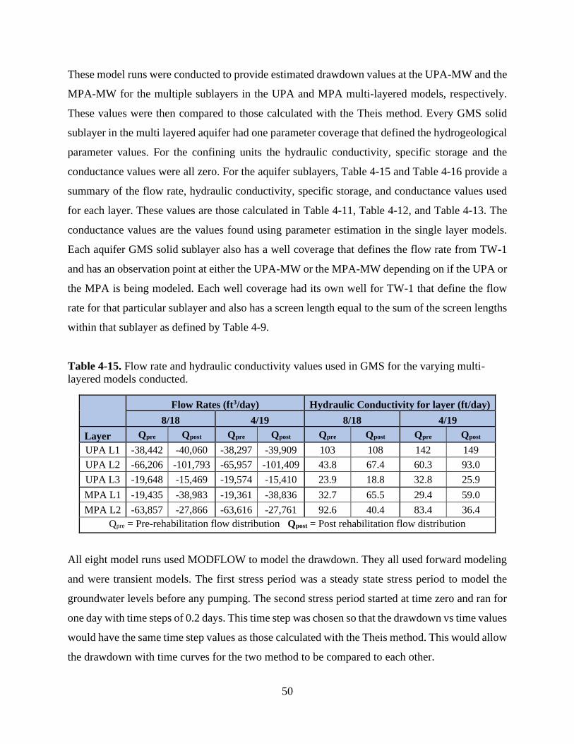
50
These model runs were conducted to provide estimated drawdown values at the UPA-MW and the
MPA-MW for the multiple sublayers in the UPA and MPA multi-layered models, respectively.
These values were then compared to those calculated with the Theis method. Every GMS solid
sublayer in the multi layered aquifer had one parameter coverage that defined the hydrogeological
parameter values. For the confining units the hydraulic conductivity, specific storage and the
conductance values were all zero. For the aquifer sublayers, Table 4-15 and Table 4-16 provide a
summary of the flow rate, hydraulic conductivity, specific storage, and conductance values used
for each layer. These values are those calculated in Table 4-11, Table 4-12, and Table 4-13. The
conductance values are the values found using parameter estimation in the single layer models.
Each aquifer GMS solid sublayer also has a well coverage that defines the flow rate from TW-1
and has an observation point at either the UPA-MW or the MPA-MW depending on if the UPA or
the MPA is being modeled. Each well coverage had its own well for TW-1 that define the flow
rate for that particular sublayer and also has a screen length equal to the sum of the screen lengths
within that sublayer as defined by Table 4-9.
Table 4-15. Flow rate and hydraulic conductivity values used in GMS for the varying multi-
layered models conducted.
Flow Rates (ft3/day) Hydraulic Conductivity for layer (ft/day)
8/18 4/19 8/18 4/19
Layer Qpre Qpost Qpre Qpost Qpre Qpost Qpre Qpost
UPA L1 -38,442 -40,060 -38,297 -39,909 103 108 142 149
UPA L2 -66,206 -101,793 -65,957 -101,409 43.8 67.4 60.3 93.0
UPA L3 -19,648 -15,469 -19,574 -15,410 23.9 18.8 32.8 25.9
MPA L1 -19,435 -38,983 -19,361 -38,836 32.7 65.5 29.4 59.0
MPA L2 -63,857 -27,866 -63,616 -27,761 92.6 40.4 83.4 36.4
Qpre = Pre-rehabilitation flow distribution Qpost = Post rehabilitation flow distribution
All eight model runs used MODFLOW to model the drawdown. They all used forward modeling
and were transient models. The first stress period was a steady state stress period to model the
groundwater levels before any pumping. The second stress period started at time zero and ran for
one day with time steps of 0.2 days. This time step was chosen so that the drawdown vs time values
would have the same time step values as those calculated with the Theis method. This would allow
the drawdown with time curves for the two method to be compared to each other.
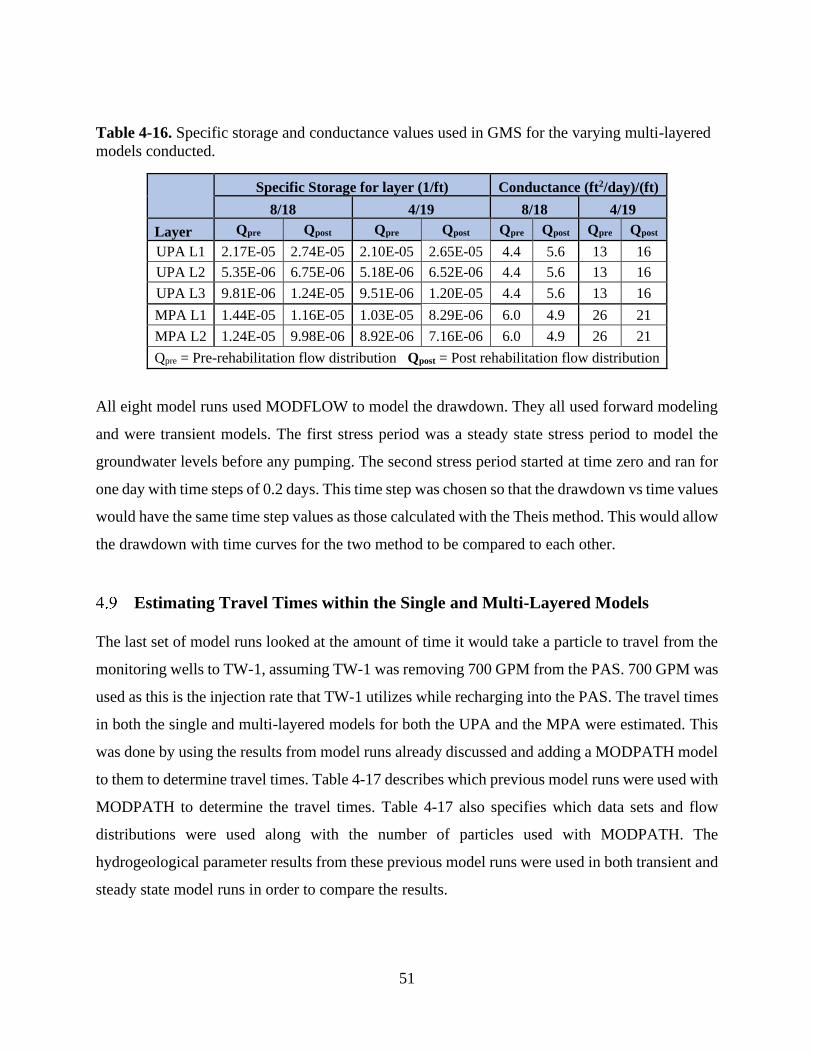
51
Table 4-16. Specific storage and conductance values used in GMS for the varying multi-layered
models conducted.
Specific Storage for layer (1/ft) Conductance (ft2/day)/(ft)
8/18 4/19 8/18 4/19
Layer Qpre Qpost Qpre Qpost Qpre Qpost Qpre Qpost
UPA L1 2.17E-05 2.74E-05 2.10E-05 2.65E-05 4.4 5.6 13 16
UPA L2 5.35E-06 6.75E-06 5.18E-06 6.52E-06 4.4 5.6 13 16
UPA L3 9.81E-06 1.24E-05 9.51E-06 1.20E-05 4.4 5.6 13 16
MPA L1 1.44E-05 1.16E-05 1.03E-05 8.29E-06 6.0 4.9 26 21
MPA L2 1.24E-05 9.98E-06 8.92E-06 7.16E-06 6.0 4.9 26 21
Qpre = Pre-rehabilitation flow distribution Qpost = Post rehabilitation flow distribution
All eight model runs used MODFLOW to model the drawdown. They all used forward modeling
and were transient models. The first stress period was a steady state stress period to model the
groundwater levels before any pumping. The second stress period started at time zero and ran for
one day with time steps of 0.2 days. This time step was chosen so that the drawdown vs time values
would have the same time step values as those calculated with the Theis method. This would allow
the drawdown with time curves for the two method to be compared to each other.
Estimating Travel Times within the Single and Multi-Layered Models
The last set of model runs looked at the amount of time it would take a particle to travel from the
monitoring wells to TW-1, assuming TW-1 was removing 700 GPM from the PAS. 700 GPM was
used as this is the injection rate that TW-1 utilizes while recharging into the PAS. The travel times
in both the single and multi-layered models for both the UPA and the MPA were estimated. This
was done by using the results from model runs already discussed and adding a MODPATH model
to them to determine travel times. Table 4-17 describes which previous model runs were used with
MODPATH to determine the travel times. Table 4-17 also specifies which data sets and flow
distributions were used along with the number of particles used with MODPATH. The
hydrogeological parameter results from these previous model runs were used in both transient and
steady state model runs in order to compare the results.

52
Table 4-17. The models focusing on estimating travel times in both single and multi-layered
aquifer models.
Model #
-Run # °
Data
Set
Used
Flow Rate
Distribution
Model
Type
Run
Option
Hydrogeological
Parameters
values
Number of
MODFLOW
Particles
1-15 8/18 Pre Transient Forward From 1-3 2
1-16 8/18 Pre Steady State Forward From 1-3 2
3-5 8/18 Pre Transient Forward From 3-1 6
3-6 8/18 Pre Steady State Forward From 3-1 6
1-17 4/19 Post Transient Forward From 1-14 2
1-18 4/19 Post Steady State Forward From 1-14 2
3-7 4/19 Post Transient Forward From 3-4 6
3-8 4/19 Post Steady State Forward From 3-4 6
2-15 8/18 Pre Transient Forward From 2-3 2
2-16 8/18 Pre Steady State Forward From 2-3 2
4-5 8/18 Pre Transient Forward From 4-1 4
4-6 8/18 Pre Steady State Forward From 4-1 4
2-17 4/19 Post Transient Forward From 2-14 2
2-18 4/19 Post Steady State Forward From 2-14 2
4-7 4/19 Post Transient Forward From 4-4 4
4-8 4/19 Post Steady State Forward From 4-4 4
° Model # 1 represents UPA single layer model, Model # 2 represents MPA single layer model,
Model # 3 represents UPA multi-layered model, Model # 4 represents MPA multi-layered model.
The pumping rate at TW-1 for all models is 700 GPM
The transient model runs had two stress periods. The first was a steady-state stress period that
modeled the groundwater before any pumping. The second stress period started at time zero and
goes for 12,000 days with 400 time steps. MODPATH was used by placing one particle within the
cell in which the SWIFT and USGS MWs are located. For the UPA models, the UPA-MW was
used and for the MPA the MPA-MW was used. Before the particles were placed, the correct layer
had to be selected to ensure the particle was placed within the correct aquifer layers and not the
confining layers. For the single layered models only two particles were needed. For the multi-
layered UPA models, six were needed, two for each aquifer sublayer. For the multi-layered MPA
models, four were needed, again two for each aquifer sublayer. Once the particles were placed and
MODFLOW had run, the travel times for each particle could be calculated and the results could
be obtained. Figure 4-16 below provides a visual example of the particle tracking function in
MODPATH. There are three path lines for each MW site as this is a model of the UPA with the
three sublayers.

53
Figure 4-16. Travel time path lines from the UPA-MW and the USGS-MW to TW-1 (From the
8/18 pre-flow UPA multi-layered model).
Finally, the impact that refinement around TW-1 had on travel times was analyzed. This was done
by rotating the location of the SWIFT and USGS particles until they were within the cells impacted
by refinement as seen in Figure 4-16. This resulted in the particle have to travel about the same
distance to TW-1 as they did from the SWIFT and USGS MW’s. However, now the particles
traveled through the cells that were affected by the refinement. The affect the refined cells had on
travel time can be seen in section 5.2.3.

54
5 Results and Discussion
Pump Test Analysis with Theis and Cooper-Jacob Methods
Table 5-1 below display the results of the calculations described in section 4.3 of this report for
the 8/18 pre-rehabilitation flow distribution and the 4/19 post rehabilitation flow distribution for
the SWIFT and USGS MW’s. The results for the 8/18 post rehabilitation flow distribution and the
4/19 pre-rehabilitation flow distribution for the SWIFT and USGS MWs can be seen in Table A-10
in the Appendix and are for comparison and validation purposes. Table 5-1 shows the results of
the realistic combinations for the data sets and the flow distributions, as the 8/18 data set took
place pre-rehabilitation and the 4/19 data set took place after rehabilitation at TW-1. When looking
at the SWIFT MW’s, the results are very similar when comparing the results of the Theis and
Cooper-Jacob methods for the same aquifer layer with the same data set and flow distribution. The
hydraulic conductivity values all fall within 4 ft/day of each other while the specific storage values
are within 1.3E-6 ft-1 of each other. These numbers help verify that the methods were utilized
correctly as they used the same data set and should result in very similar values. The slight
differences are likely due to human interpretation when it comes to where the graphs line up with
the Theis method and where the linear line should be placed for the Cooper-Jacob method.
Comparing results derived from the SWIFT MW data to the USGS MW, the USGS hydraulic
conductivity results that could be obtained differed slightly from the SWIFT MW results, with the
smallest difference in hydraulic conductivity values being 15 ft/day. However, this difference is
within reason as the results are within the same order of magnitude, which is reasonable when
comparing hydraulic conductivity. The specific storage results were closer in values with all but
one of the results being outside of one order of magnitude of the SWIFT MW results. While the
USGS results differ from the SWIFT results, the differences are within reason given the large
range in possible values for both hydraulic conductivity and specific storage. However, as
discussed earlier, only a small number of the USGS data sets were usable with the Theis and
Cooper-Jacob methods. For the data sets that were not usable, as seen in Figure A-13 through
Figure A-19, their log-log plots were compared to other diagnostic plots. The 8/18 USGS-MPA
data set was the only data that had any resemblance to a diagnostic plot, that being the plot for
double porosity aquifers (Renard et al., 2009). However, this resemblance is likely due to the
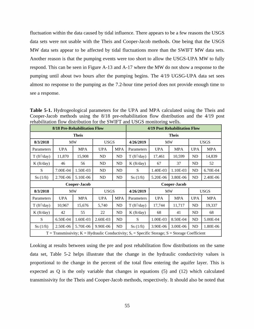
55
fluctuation within the data caused by tidal influence. There appears to be a few reasons the USGS
data sets were not usable with the Theis and Cooper-Jacob methods. One being that the USGS
MW data sets appear to be affected by tidal fluctuations more than the SWIFT MW data sets.
Another reason is that the pumping events were too short to allow the USGS-UPA MW to fully
respond. This can be seen in Figure A-13 and A-17 where the MW do not show a response to the
pumping until about two hours after the pumping begins. The 4/19 UGSG-UPA data set sees
almost no response to the pumping as the 7.2-hour time period does not provide enough time to
see a response.
Table 5-1. Hydrogeological parameters for the UPA and MPA calculated using the Theis and
Cooper-Jacob methods using the 8/18 pre-rehabilitation flow distribution and the 4/19 post
rehabilitation flow distribution for the SWIFT and USGS monitoring wells.
8/18 Pre-Rehabilitation Flow 4/19 Post Rehabilitation Flow
Theis Theis
8/3/2018 MW USGS 4/26/2019 MW USGS
Parameters UPA MPA UPA MPA Parameters UPA MPA UPA MPA
T (ft2/day) 11,870 15,908 ND ND T (ft2/day) 17,461 10,599 ND 14,839
K (ft/day) 46 56 ND ND K (ft/day) 67 37 ND 52
S 7.00E-04 1.50E-03 ND ND S 1.40E-03 1.10E-03 ND 6.70E-04
Ss (1/ft) 2.70E-06 5.10E-06 ND ND Ss (1/ft) 5.20E-06 3.80E-06 ND 2.40E-06
Cooper-Jacob Cooper-Jacob
8/3/2018 MW USGS 4/26/2019 MW USGS
Parameters UPA MPA UPA MPA Parameters UPA MPA UPA MPA
T (ft2/day) 10,967 15,676 5,740 ND T (ft2/day) 17,744 11,717 ND 19,337
K (ft/day) 42 55 22 ND K (ft/day) 68 41 ND 68
S 6.50E-04 1.60E-03 2.60E-03 ND S 1.00E-03 8.50E-04 ND 5.00E-04
Ss (1/ft) 2.50E-06 5.70E-06 9.90E-06 ND Ss (1/ft) 3.90E-06 3.00E-06 ND 1.80E-06
T = Transmissivity; K = Hydraulic Conductivity; Ss = Specific Storage; S = Storage Coefficient
Looking at results between using the pre and post rehabilitation flow distributions on the same
data set, Table 5-2 helps illustrate that the change in the hydraulic conductivity values is
proportional to the change in the percent of the total flow entering the aquifer layer. This is
expected as Q is the only variable that changes in equations (5) and (12) which calculated
transmissivity for the Theis and Cooper-Jacob methods, respectively. It should also be noted that

56
the thickness of the layer, b, does not change when calculating hydraulic conductivity from
transmissivity and therefore does not affect the ratio.
Table 5-2. Ratio of hydraulic conductivity (K) over percent of total flow for the UPA or MPA of
the Potomac Aquifer for both the Theis and Cooper-Jacob methods with various data set and flow
distribution combinations. K (ft/day) % of Total Flow Ratio (K/% of Total Flow)
UPA Theis 8/18 Pre-Flow 46 58 0.79
Post Flow 58 74 0.78
UPA C-J 8/18 Pre-Flow 42 58 0.72
Post Flow 55 74 0.74
UPA Theis 4/19 Pre-Flow 53 58 0.91
Post Flow 67 74 0.91
UPA C-J 4/19 Pre-Flow 54 58 0.93
Post Flow 68 74 0.92
MPA Theis 8/18 Pre-Flow 56 39 1.44
Post Flow 45 31 1.45
MPA C-J 8/18 Pre-Flow 55 39 1.41
Post Flow 44 31 1.42
MPA Theis 4/19 Pre-Flow 47 39 1.21
Post Flow 37 31 1.19
MPA C-J 4/19 Pre-Flow 52 39 1.33
Post Flow 41 31 1.32
These calculated hydrogeological parameters can be compared to those discussed in the literature
review. Table 5-3 provides a summary of the K and T values from the sources in the literature
review. If it is assumed that the LPA transmissivity is significantly lower than that of the UPA and
the MPA, than it can be assumed that the sum of the transmissivity values for the UPA and the
MPA is equal to the overall Potomac aquifer transmissivity value. Using the SWIFT MW results,
the sum of the UPA and the MPA transmissivity values fall between 25,000 and 30,000 ft2/day
which is greater than that reported in Trapp Jr. and Horn (1997) but within reason. The
transmissivity values for each individual layer of the Potomac aquifer provided in Lucas (2016)
are significantly lower than those calculated in this research. However, the overall transmissivity
provided in Lucas (2016) is significantly greater than the sum of the transmissivity values of the
three layers and places these values into question. The transmissivity values for the UPA, MPA,
and LPA provided in Lucas (2016) are based on a packer test within TW-1 and only utilize water
level data from TW-1. Whereas the PAS transmissivity value from Lucas (2016) is based on a 24-
hour constant rate pump test that utilized data from MW’s. Based on how their results compare to
this research and past research, the pump tests utilizing MW water level data and not just TW-1

57
water level data provided better results. The overall transmissivity value provided by Lucas (2016)
is within the range provided in Trapp Jr. and Horn (1997). The hydraulic conductivity values
provided in Smith (1999) are very close in value to the results of the 4/19 post-rehabilitation flow
distribution calculated results. The Smith (1999) values say that the UPA has a higher K value than
the MPA which contradicts the 8/18 pre-rehabilitation flow distribution calculated results. As a
result of this contradiction along with the 4/19 post flow values being the most current, the
calculated 4/19 post flow results should be used for future studies of this site.
Table 5-3. Summary of the hydraulic conductivity and transmissivity values for the Potomac
aquifer found within past research and literature compared to the Theis and Cooper-Jacob method
results.
Hydrogeologic
al Parameters
Smith,
1999
Heywood &
Pope, 2009
Lucas,
2016
Trapp Jr.
& Horn,
1997
Calculated
average (8/18
pre-rehab.)*
Calculated
average (4/19
post rehab.)*
UPA T
(ft2/day) - - 3,514 - 11,418 17,602
UPA K (ft/day) 74.1 - - - 44 68
MPA T
(ft2/day) - - 2,835 - 15,792 11,158
MPA K
(ft/day) 40 - - - 56 39
Potomac
Aquifer T
(ft2/day)
- - 19,100 10,000 to
20,000 27,210+ 28,760+
Potomac
Aquifer K
(ft/day)
35.01 to 50 - - 58+ 61+
*Based on Theis and Cooper-Jacob calculations on the SWIFT MW observation data only. +Values only based on UPA and MPA, LPA is not included.
T = Transmissivity K = Hydraulic Conductivity
GMS Model Results
Hydrogeological Parameter Estimation
For the purposes of this research, the gradient and direction of flow for the MPA is assumed to be
the same as that calculated for the UPA. The sensitivities for each of the hydrogeological
parameters estimated with parameter estimation can be seen in Figure 5-1 through Figure 5-3.
These figures only show the sensitivity results for the UPA and MPA 8/18 pre-rehabilitation flow

58
rate model run and the MPA 4/19 post rehabilitation flow rate model run. The remaining sensitivity
results can be seen in the Appendix. These three figures were chosen as they summarize the
sensitivities for the three parameters for the UPA and MPA models. Figure 5-1 shows that for
every model run of the UPA the hydraulic conductivity affected the model the most while
conductance had the smallest impact on the model run results. For the MPA model runs using the
4/19 data set, the sensitivity values are summarized in Figure 5-2. For these model runs the
conductance still has a smaller impact on the model run results. Figure 5-3 summarizes the
sensitivity values for the MPA model runs using the 8/18 data set. For these model runs the
hydraulic conductivity still has the greatest effect on the model results. However, the specific
storage and conductance have a relatively higher and near equal impact on the models results
compared to the UPA. The change in the conductance’s sensitivity values between the different
model runs can be explained by the difference in the radius of the cone of influence produced by
pumping at TW-1. Figure 5-4 shows the cone of influence for the UPA 8/18 data set, pre-
rehabilitation flow distribution model run. Figure 5-5 shows the cone of influence for the MPA
8/18 data set, pre-rehabilitation flow distribution model run. When these two figures are compared,
the UPA model run has smaller change in head values at the boundaries of the model (around -0.4
feet) compared to the MPA model run using the 8/18 data set (around -1 feet). Figure 5-4 also
shows that the rate at which the change in head values approach zero moving away from TW-1 is
greater than that seen in Figure 5-5. This can be seen as the change in head goes from -20 feet at
TW-1 to about -0.4 feet at the boundaries of the model for Figure 5-4. Whereas the head goes from
-6.4 feet at TW-1 to about -1 feet at the boundaries of the model for Figure 5-5. This implies that
the cone of influence for the MPA model runs using the 8/18 data set extends much further past
the boundaries then for the UPA model runs or for the MPA model runs using the 4/19 data set.
The larger cone of influence would result in the conductance value having a greater impact on the
model.

59
Figure 5-1. Sensitivity of the estimated parameters within the 8/18 pre-flow UPA single layer
model using PEST (1-2).
Figure 5-2. Sensitivity of the estimated parameters within the 4/19 post flow MPA single layer
model using PEST (2-13).
Figure 5-3. Sensitivity of the estimated parameters within the 8/18 pre-flow MPA single layer
model using PEST (2-2).
8.85E-02
2.29E-02
2.77E-05
0.0E+00
1.0E-02
2.0E-02
3.0E-02
4.0E-02
5.0E-02
6.0E-02
7.0E-02
8.0E-02
9.0E-02
1.0E-01
Hydraulic Conductivity(ft/Day)
Specific Storage (1/ft) Conductance(ft^2/Day)/(ft)
Sen
siti
vity
Sensitivity of UPA 8/18 Data Modeled with Pre-rehab Flow Rate
1.79E-02
6.16E-03
1.63E-03
0.0E+00
2.0E-03
4.0E-03
6.0E-03
8.0E-03
1.0E-02
1.2E-02
1.4E-02
1.6E-02
1.8E-02
2.0E-02
Hydraulic Conductivity(ft/Day)
Specific Storage (1/ft) Conductance(ft^2/Day)/(ft)
Sen
siti
vity
Sensitivity of MPA 4/19 Data Modeled with Post Rehab Flow Rate
2.40E-02
1.21E-021.10E-02
0.0E+00
5.0E-03
1.0E-02
1.5E-02
2.0E-02
2.5E-02
3.0E-02
Hydraulic Conductivity(ft/Day)
Specific Storage (1/ft) Conductance(ft^2/Day)/(ft)
Sen
siti
vity
Sensitivity of MPA 8/18 Data Modeled with Pre-rehab Flow Rate
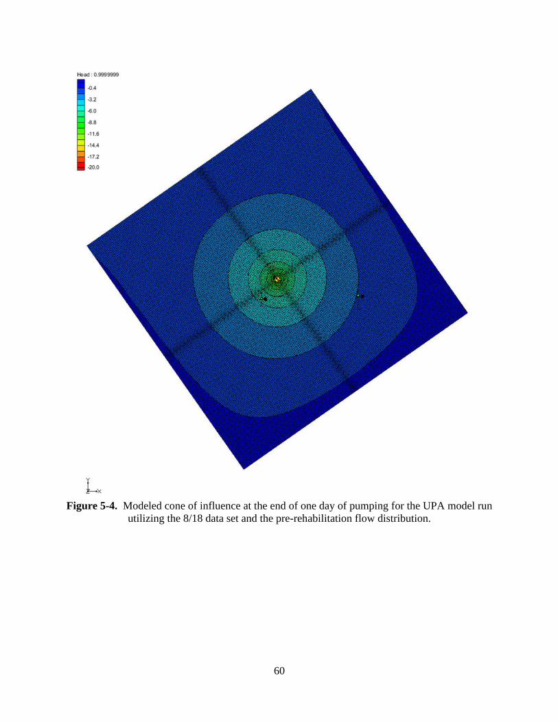
60
Figure 5-4. Modeled cone of influence at the end of one day of pumping for the UPA model run
utilizing the 8/18 data set and the pre-rehabilitation flow distribution.

61
Figure 5-5. Modeled cone of influence at the end of one day of pumping for the MPA model run
utilizing the 8/18 data set and the pre-rehabilitation flow distribution.
Table 5-4 provides an example of how the uniqueness of the models were tested to ensure the
model converges on the same result regardless of the initial values. The difference in conductance
values is expected considering the low sensitivity value for conductance. The uniqueness tables
for the other model results can be seen in the Appendix as Table A-12 through Table A-18.

62
Table 5-4. Uniqueness of the model results using the PEST package with two separate model
runs for the 8/18 pre-flow UPA single layer model.
UPA 8/18 Data Modeled with Pre-rehabilitation Flow Rate Uniqueness (1-2)
High Initial Values Low Initial Values
Parameter Initial
Values
Final
Values Parameter
Initial
Values
Final
Values
K (ft/Day) 80 27.3 K (ft/Day) 10 27.3
Ss (1/ft) 1.00E-04 5.85E-06 Ss (1/ft) 1.00E-07 5.86E-06
Conductance
(ft2/Day)/(ft) 10000 9999
Conductance
(ft2/Day)/(ft) 1 5350
K = Hydraulic Conductivity Ss = Specific Storage
Table 5-5 provides a summary of the hydrogeological parameters determined from models 1 and
2 (single layer) runs. From the discussion on the low conductance sensitivity values for the UPA
models, the large fluctuation seen in the conductance values for UPA model runs is not alarming.
Figure A-25 through Figure A-52 in the Appendix show the modeled vs observed drawdown vs
time for each model run for the single layered model runs. For the forward model runs, the modeled
and observed drawdown curves do not overlap which confirms that the hydrogeological
parameters calculated from one data set (8/18 or 4/19) cannot be used to model the over data sets
observation data. This is expected as rehabilitation of TW-1 took place between these two data
sets.
Looking at the impact the change in the weighting of the SWIFT MW data had on the results for
the parameter estimation models. There was little change in the hydraulic conductivity or the
specific storage for the MPA models when the weighting was changed from one to four. Only the
4/19 data set models for the UPA saw a drastic change in the hydraulic conductivity and specific
storage values. This large change is not surprising as the 4/19 UPA USGS MW data seen in Figure
A-17 in the Appendix has the worst response to the pump test, as previously discussed. When
comparing the model runs that used the USGS MW data to the runs that do not, there is a change
in hydraulic conductivity and specific storage values. However, this difference is again within
reason for these parameters. But these differences in the results do imply that the USGS MW data
differs in its response to the pump tests, which could be due to tidal influences as previously
discussed or other factors. For the UPA, the increase in the hydraulic conductivity and specific
storage values, when the USGS MW data are not considered, could be due to an unknown obstacle
or a low transmissivity zone within the aquifer unit located between TW-1 and the USGS

63
monitoring wells. For the MPA the decrease in the hydraulic conductivity and specific storage
values, when the USGS MW data are not considered, could be due to a high transmissivity zone
within the aquifer unit located between TW-1 and the USGS monitoring wells. However, for the
MPA, the change in the hydraulic conductivity and specific storage values when the USGS MW
data are not considered, is much smaller compared to the UPA.
Table 5-5. Summary of the final parameter found with parameter estimation for the 28 models
varying with which aquifer layer, data set, weighting, and flow distribution was used.
Modeled Hydrogeological Parameters for Both Data Set
Model
# -
Run #
°
Model type
Data
Set
Used
Flow Data
Used
USGS
Standard
Dev.
SWIFT
MW Ob.
Point
Weighting
K
(ft/Day) Ss (1/ft)
Conductance
(ft2/Day)/(ft)
T
(ft2/day)
1-1 Parameter Est. 8/18 Pre-rehab. 1 1 26 7.4E-06 24,292 6,839
1-2 Parameter Est. 8/18 Pre-rehab. 1 4 27 5.9E-06 5,350 7,108
1-3 Parameter Est. 8/18 Pre-rehab. NA 1 42 2.8E-06 4 11,022
1-4 Parameter Est. 8/18 Post-rehab. 1 1 33 9.4E-06 12,492 8,634
1-5 Parameter Est. 8/18 Post-rehab. 1 4 35 7.4E-06 4,779 8,997
1-6 Parameter Est. 8/18 Post-rehab. NA 1 54 3.5E-06 6 13,966
1-7 Forward 4/19 Pre-rehab. NA NA 27 5.9E-06 5,350 7,108
1-8 Parameter Est. 4/19 Pre-rehab. 1 1 32 1.1E-05 31,250 8,398
1-9 Parameter Est. 4/19 Pre-rehab. 1 4 46 4.5E-06 7,366 11,916
1-10 Parameter Est. 4/19 Pre-rehab. NA 1 58 2.7E-06 13 15,166
1-11 Forward 4/19 Post-rehab. NA NA 35 7.4E-06 4,779 8,997
1-12 Parameter Est. 4/19 Post-rehab. 1 1 41 1.4E-05 31,251 10,643
1-13 Parameter Est. 4/19 Post-rehab. 1 4 58 5.7E-06 6,632 15,084
1-14 Parameter Est. 4/19 Post-rehab. NA 1 74 3.4E-06 16 19,265
2-1 Parameter Est. 8/18 Pre-rehab. 1 1 63 4.8E-06 5 16,351
2-2 Parameter Est. 8/18 Pre-rehab. 1 4 63 4.9E-06 5 16,297
2-3 Parameter Est. 8/18 Pre-rehab. NA 1 58 5.4E-06 6 14,982
2-4 Parameter Est. 8/18 Post-rehab. 1 1 50 3.9E-06 4 13,123
2-5 Parameter Est. 8/18 Post-rehab. 1 4 50 3.9E-06 4 13,080
2-6 Parameter Est. 8/18 Post-rehab. NA 1 46 4.4E-06 5 12,027
2-7 Forward 4/19 Pre-rehab. NA NA 63 4.9E-06 5 16,297
2-8 Parameter Est. 4/19 Pre-rehab. 1 1 53 3.6E-06 28 13,795
2-9 Parameter Est. 4/19 Pre-rehab. 1 4 52 3.8E-06 26 13,638
2-10 Parameter Est. 4/19 Pre-rehab. NA 1 52 3.9E-06 26 13,485
2-11 Forward 4/19 Post-rehab. NA NA 50 3.9E-06 4 13,080
2-12 Parameter Est. 4/19 Post-rehab. 1 1 43 2.9E-06 23 11,071
2-13 Parameter Est. 4/19 Post-rehab. 1 4 42 3.0E-06 21 10,946
2-14 Parameter Est. 4/19 Post-rehab. NA 1 42 3.1E-06 21 10,824
T = Transmissivity K = Hydraulic Conductivity Ss = Specific Storage
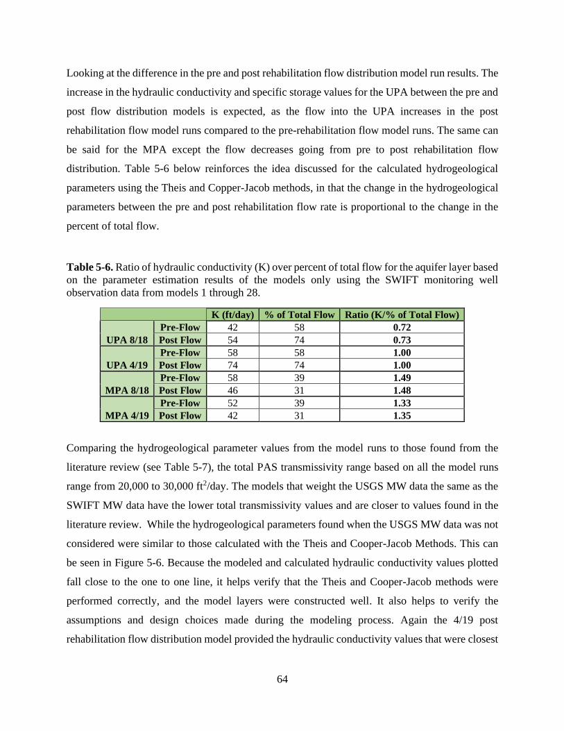
64
Looking at the difference in the pre and post rehabilitation flow distribution model run results. The
increase in the hydraulic conductivity and specific storage values for the UPA between the pre and
post flow distribution models is expected, as the flow into the UPA increases in the post
rehabilitation flow model runs compared to the pre-rehabilitation flow model runs. The same can
be said for the MPA except the flow decreases going from pre to post rehabilitation flow
distribution. Table 5-6 below reinforces the idea discussed for the calculated hydrogeological
parameters using the Theis and Copper-Jacob methods, in that the change in the hydrogeological
parameters between the pre and post rehabilitation flow rate is proportional to the change in the
percent of total flow.
Table 5-6. Ratio of hydraulic conductivity (K) over percent of total flow for the aquifer layer based
on the parameter estimation results of the models only using the SWIFT monitoring well
observation data from models 1 through 28.
K (ft/day) % of Total Flow Ratio (K/% of Total Flow)
UPA 8/18
Pre-Flow 42 58 0.72
Post Flow 54 74 0.73
UPA 4/19
Pre-Flow 58 58 1.00
Post Flow 74 74 1.00
MPA 8/18
Pre-Flow 58 39 1.49
Post Flow 46 31 1.48
MPA 4/19
Pre-Flow 52 39 1.33
Post Flow 42 31 1.35
Comparing the hydrogeological parameter values from the model runs to those found from the
literature review (see Table 5-7), the total PAS transmissivity range based on all the model runs
range from 20,000 to 30,000 ft2/day. The models that weight the USGS MW data the same as the
SWIFT MW data have the lower total transmissivity values and are closer to values found in the
literature review. While the hydrogeological parameters found when the USGS MW data was not
considered were similar to those calculated with the Theis and Cooper-Jacob Methods. This can
be seen in Figure 5-6. Because the modeled and calculated hydraulic conductivity values plotted
fall close to the one to one line, it helps verify that the Theis and Cooper-Jacob methods were
performed correctly, and the model layers were constructed well. It also helps to verify the
assumptions and design choices made during the modeling process. Again the 4/19 post
rehabilitation flow distribution model provided the hydraulic conductivity values that were closest
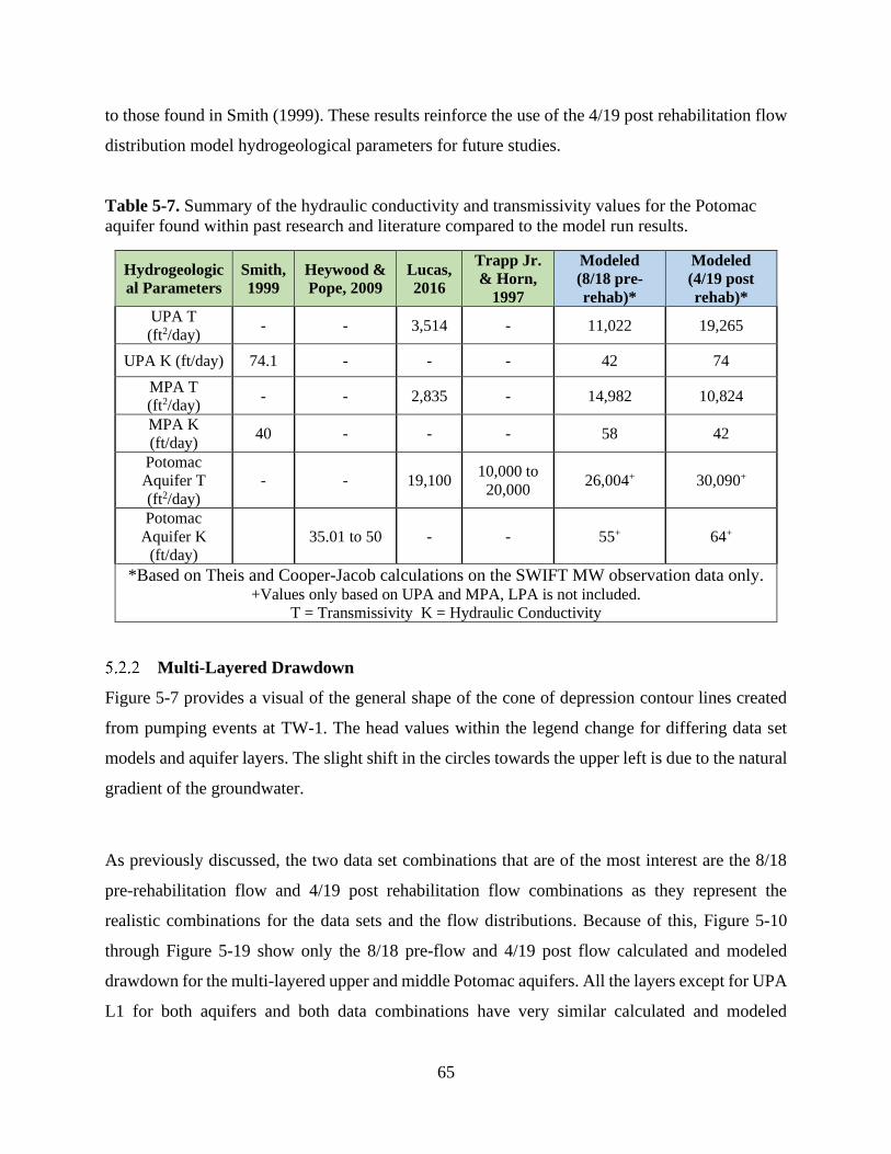
65
to those found in Smith (1999). These results reinforce the use of the 4/19 post rehabilitation flow
distribution model hydrogeological parameters for future studies.
Table 5-7. Summary of the hydraulic conductivity and transmissivity values for the Potomac
aquifer found within past research and literature compared to the model run results.
Hydrogeologic
al Parameters
Smith,
1999
Heywood &
Pope, 2009
Lucas,
2016
Trapp Jr.
& Horn,
1997
Modeled
(8/18 pre-
rehab)*
Modeled
(4/19 post
rehab)*
UPA T
(ft2/day) - - 3,514 - 11,022 19,265
UPA K (ft/day) 74.1 - - - 42 74
MPA T
(ft2/day) - - 2,835 - 14,982 10,824
MPA K
(ft/day) 40 - - - 58 42
Potomac
Aquifer T
(ft2/day)
- - 19,100 10,000 to
20,000 26,004+ 30,090+
Potomac
Aquifer K
(ft/day)
35.01 to 50 - - 55+ 64+
*Based on Theis and Cooper-Jacob calculations on the SWIFT MW observation data only. +Values only based on UPA and MPA, LPA is not included.
T = Transmissivity K = Hydraulic Conductivity
Multi-Layered Drawdown
Figure 5-7 provides a visual of the general shape of the cone of depression contour lines created
from pumping events at TW-1. The head values within the legend change for differing data set
models and aquifer layers. The slight shift in the circles towards the upper left is due to the natural
gradient of the groundwater.
As previously discussed, the two data set combinations that are of the most interest are the 8/18
pre-rehabilitation flow and 4/19 post rehabilitation flow combinations as they represent the
realistic combinations for the data sets and the flow distributions. Because of this, Figure 5-10
through Figure 5-19 show only the 8/18 pre-flow and 4/19 post flow calculated and modeled
drawdown for the multi-layered upper and middle Potomac aquifers. All the layers except for UPA
L1 for both aquifers and both data combinations have very similar calculated and modeled
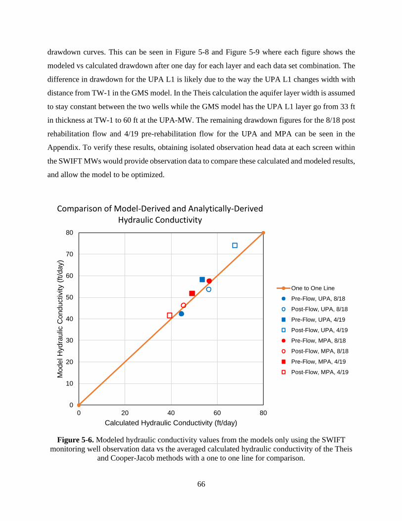
66
drawdown curves. This can be seen in Figure 5-8 and Figure 5-9 where each figure shows the
modeled vs calculated drawdown after one day for each layer and each data set combination. The
difference in drawdown for the UPA L1 is likely due to the way the UPA L1 changes width with
distance from TW-1 in the GMS model. In the Theis calculation the aquifer layer width is assumed
to stay constant between the two wells while the GMS model has the UPA L1 layer go from 33 ft
in thickness at TW-1 to 60 ft at the UPA-MW. The remaining drawdown figures for the 8/18 post
rehabilitation flow and 4/19 pre-rehabilitation flow for the UPA and MPA can be seen in the
Appendix. To verify these results, obtaining isolated observation head data at each screen within
the SWIFT MWs would provide observation data to compare these calculated and modeled results,
and allow the model to be optimized.
Figure 5-6. Modeled hydraulic conductivity values from the models only using the SWIFT
monitoring well observation data vs the averaged calculated hydraulic conductivity of the Theis
and Cooper-Jacob methods with a one to one line for comparison.
0
10
20
30
40
50
60
70
80
0 20 40 60 80
Mo
de
l H
yd
rau
lic C
ond
uctivity (
ft/d
ay)
Calculated Hydraulic Conductivity (ft/day)
Comparison of Model-Derived and Analytically-Derived Hydraulic Conductivity
One to One Line
Pre-Flow, UPA, 8/18
Post-Flow, UPA, 8/18
Pre-Flow, UPA, 4/19
Post-Flow, UPA, 4/19
Pre-Flow, MPA, 8/18
Post-Flow, MPA, 8/18
Pre-Flow, MPA, 4/19
Post-Flow, MPA, 4/19
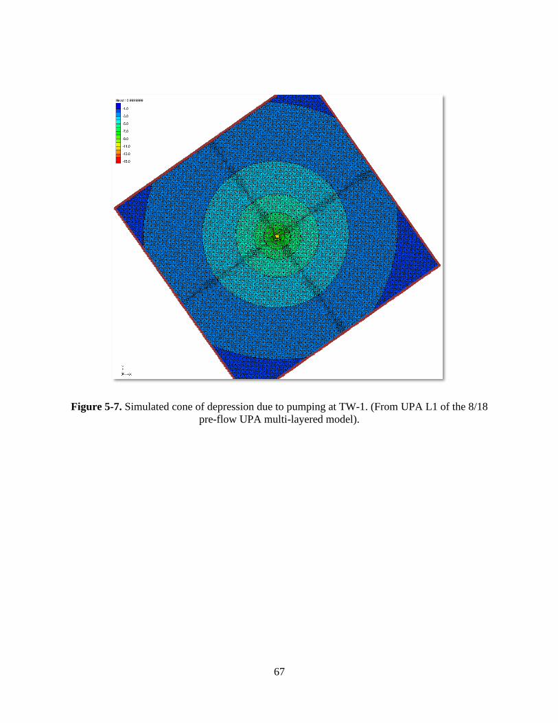
67
Figure 5-7. Simulated cone of depression due to pumping at TW-1. (From UPA L1 of the 8/18
pre-flow UPA multi-layered model).
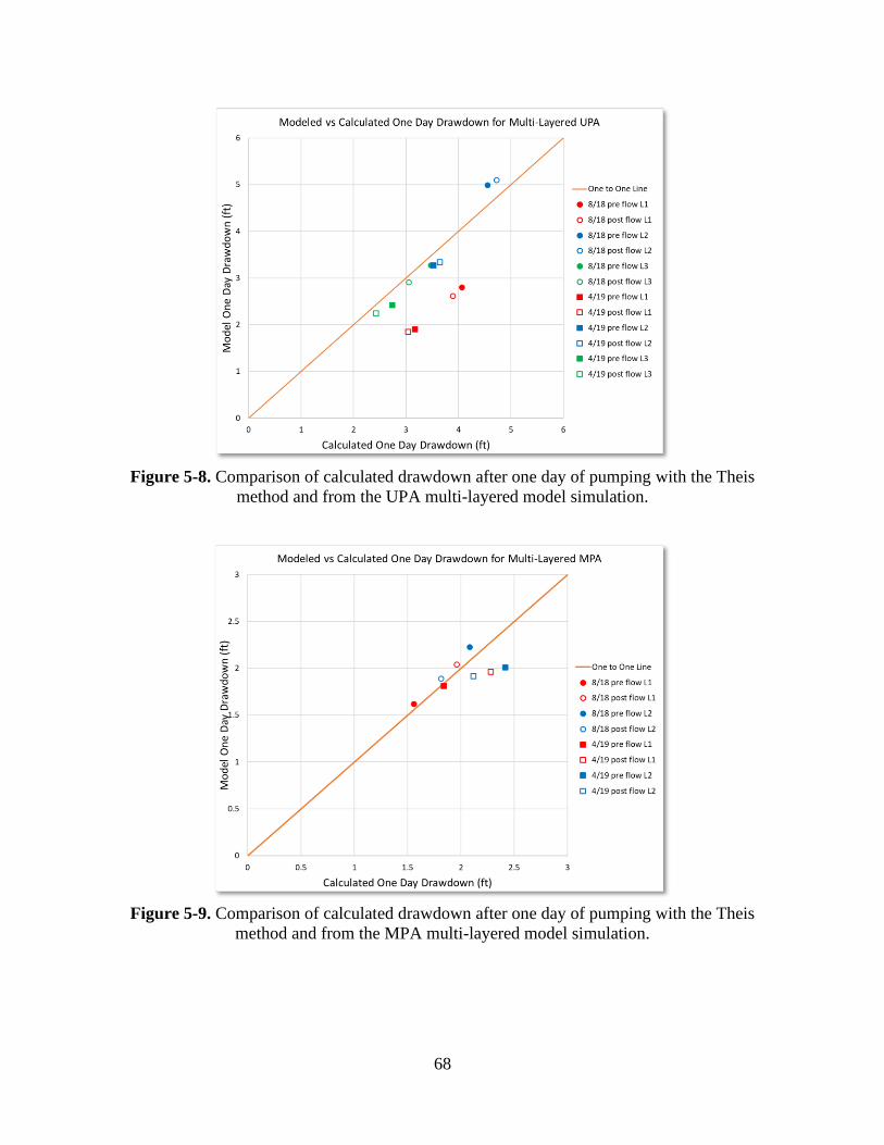
68
Figure 5-8. Comparison of calculated drawdown after one day of pumping with the Theis
method and from the UPA multi-layered model simulation.
Figure 5-9. Comparison of calculated drawdown after one day of pumping with the Theis
method and from the MPA multi-layered model simulation.
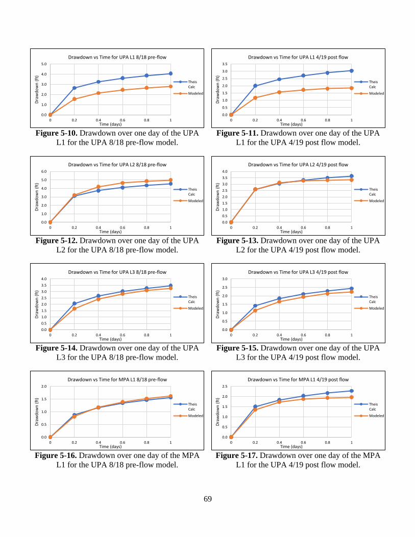
69
Figure 5-10. Drawdown over one day of the UPA
L1 for the UPA 8/18 pre-flow model.
Figure 5-11. Drawdown over one day of the UPA
L1 for the UPA 4/19 post flow model.
Figure 5-12. Drawdown over one day of the UPA
L2 for the UPA 8/18 pre-flow model.
Figure 5-13. Drawdown over one day of the UPA
L2 for the UPA 4/19 post flow model.
Figure 5-14. Drawdown over one day of the UPA
L3 for the UPA 8/18 pre-flow model.
Figure 5-15. Drawdown over one day of the UPA
L3 for the UPA 4/19 post flow model.
Figure 5-16. Drawdown over one day of the MPA
L1 for the UPA 8/18 pre-flow model.
Figure 5-17. Drawdown over one day of the MPA
L1 for the UPA 4/19 post flow model.
0.0
1.0
2.0
3.0
4.0
5.0
0 0.2 0.4 0.6 0.8 1
Dra
wd
ow
n (
ft)
Time (days)
Drawdown vs Time for UPA L1 8/18 pre-flow
TheisCalc
Modeled
0.0
0.5
1.0
1.5
2.0
2.5
3.0
3.5
0 0.2 0.4 0.6 0.8 1
Dra
wd
ow
n (
ft)
Time (days)
Drawdown vs Time for UPA L1 4/19 post flow
TheisCalc
Modeled
0.0
1.0
2.0
3.0
4.0
5.0
6.0
0 0.2 0.4 0.6 0.8 1
Dra
wd
ow
n (
ft)
Time (days)
Drawdown vs Time for UPA L2 8/18 pre-flow
TheisCalc
Modeled
0.0
0.5
1.0
1.5
2.0
2.5
3.0
3.5
4.0
0 0.2 0.4 0.6 0.8 1
Dra
wd
ow
n (
ft)
Time (days)
Drawdown vs Time for UPA L2 4/19 post flow
TheisCalc
Modeled
0.0
0.5
1.0
1.5
2.0
2.5
3.0
3.5
4.0
0 0.2 0.4 0.6 0.8 1
Dra
wd
ow
n (
ft)
Time (days)
Drawdown vs Time for UPA L3 8/18 pre-flow
TheisCalc
Modeled
0.0
0.5
1.0
1.5
2.0
2.5
3.0
0 0.2 0.4 0.6 0.8 1
Dra
wd
ow
n (
ft)
Time (days)
Drawdown vs Time for UPA L3 4/19 post flow
TheisCalc
Modeled
0.0
0.5
1.0
1.5
2.0
0 0.2 0.4 0.6 0.8 1
Dra
wd
ow
n (
ft)
Time (days)
Drawdown vs Time for MPA L1 8/18 pre-flow
TheisCalc
Modeled
0.0
0.5
1.0
1.5
2.0
2.5
0 0.2 0.4 0.6 0.8 1
Dra
wd
ow
n (
ft)
Time (days)
Drawdown vs Time for MPA L1 4/19 post flow
TheisCalc
Modeled

70
Figure 5-18. Drawdown over one day of the MPA
L2 for the UPA 8/18 pre-flow model.
Figure 5-19. Drawdown over one day of the MPA
L2 for the UPA 4/19 post flow model.
Travel Times
The travel times for a particle to travel from either the UPA-MW (for UPA layers) and the MPA-
MW (for MPA layers) to TW-1 for both the 8/18 pre-flow and 4/19 post flow data combinations
can be seen in Table 5-8 and Table 5-9. These tables show only the steady state model results, as
the transient models (see Appendix) provide results that differ by no more than a day. These results
are a good initial estimate for travel times but do not consider diffusion which would affect solute
travel times in a tracer test. Looking at the 4/19 post flow values compared to the 8/18 pre-flow
values. The time change is relative to the change in the flow rate entering each layer, but they are
not proportional. When looking at the effect the fine mesh had on the travel times for a particle
traveling the same distances as if it were from the SWIFT or USGS MW’s. Table 5-10 shows how
the fine mesh does not significantly affect the travel times over the same distance. This can be seen
when the ratios for the time over distance traveled for the particles at the MWs are compared to
the ratios for the time over distance traveled for the particles along the fine mesh.
Table 5-8. Estimated travel time from the SWIFT or USGS monitoring well to TW-1 for both the
single and multi-layered steady state model layers based on the pre-rehabilitation flow, 8/18 data
set hydrogeological parameters.
Steady State 8/18 Travel Time to TW-1 (days) Pre-Rehab. Flow
Layer SWIFT MW USGS MW % of Total Flow Flow from Layer (GPM)
UPA SL 372 4,839 58 406
UPA L1 204 2,395 18 126
UPA L2 322 4,005 31 217
UPA L3 597 7,859 9.2 64.4
MPA SL 743 7,545 39 273
MPA L1 1,195 11,245 9.1 63.7
MPA L2 416 4,339 30 210
0.0
0.5
1.0
1.5
2.0
2.5
0 0.2 0.4 0.6 0.8 1
Dra
wd
ow
n (
ft)
Time (days)
Drawdown vs Time for MPA L2 8/18 pre-flow
TheisCalc
Modeled
0.0
0.5
1.0
1.5
2.0
2.5
0 0.2 0.4 0.6 0.8 1
Dra
wd
ow
n (
ft)
Time (days)
Drawdown vs Time for MPA L2 4/19 post flow
TheisCalc
Modeled

71
Table 5-9. Estimated travel time from the SWIFT or USGS monitoring well to TW-1 for both the
single and multi-layered model layers based on the post rehabilitation flow, 4/19 data set
hydrogeological parameters.
Steady State 4/19 Travel Time to TW-1 (days) Post Rehab Flow
Layer SWIFT MW USGS MW % of Total Flow Flow from Layer (GPM)
UPA SL 292 3,757 74 518
UPA L1 193 2,284 19 133
UPA L2 209 2,560 48 336
UPA L3 754 9,867 7 49
MPA SL 919 9,273 31 217
MPA L1 596 5,669 18 126
MPA L2 949 9,812 13 91
Table 5-10. Comparison of the travel times from the monitoring wells to TW-1 to the travel
times along the fine mesh.
MPA L1 From Wells Along fine Mesh
Monitoring
Wells Distance
(ft) Travel Time
(Days) Ratio of
Time/Distance Distance
(ft) Travel Time
(Days) Ratio of
Time/Distance
SWIFT 378 1195 3.16 382 1175 3.08
USGS 1266 11245 8.88 1274 11340 8.90
MPA L2
From Wells Along fine Mesh
Monitoring
Wells Distance
(ft) Travel Time
(Days) Ratio of
Time/Distance Distance
(ft) Travel Time
(Days) Ratio of
Time/Distance
SWIFT 378 416 1.10 382 409 1.07
USGS 1266 4339 3.43 1274 4290 3.37
72
6 Conclusion
Summary
From the results of this research and those from past research for the Potomac aquifer, it was found
that the use of the 4/19 post rehabilitation flow distribution provided the best hydrogeological
parameters to be used for future modeling of this site. This is because the results from this
combination of data set and flow distribution utilizes the most current data set and uses the flow
distribution that represented the distribution of flow within TW-1 at that time. These results also
closely resemble those found in past research done on the Potomac aquifer. The Theis and Cooper-
Jacob methods provided hydrogeological parameter values that nearly matched those from
Parameter estimation using the GMS models with only the SWIFT MW data. The models using
the USGS MW data had slightly differing hydrogeological parameter values but were within
reason to the results from the SWIFT MW data. The slight difference in results for the USGS MW
data are due to the MWs not responding to the pump test in a reliable way. If TW-1 undergoes
rehabilitation again in the future, new flow distributions should be determined as this change in
distribution will have a proportional impact on the change in the hydrogeological parameters for
the aquifer.
The multi-layered calculated and modeled drawdown values were similar in their values except
for UPA L1 as the modeled thickness changes with distance from TW-1. To verify these results,
obtaining isolated observation head data at each screen within the SWIFT MWs would provide
drawdown values that could be compared to these drawdown values calculated and modeled. The
travel times estimated for each layer provide good initial estimations and will help with the
planning of future studies such as tracer tests. The fine mesh within the models did not appear to
affect travel times.
This research provides hydrogeological parameter values for the PAS for the UPA and the MPA
as both single and multi-layered units on a local scale around the SWIFTRC. These values will be
used in future studies for the SWIFT project and will be added onto as the project expands in its
scale. This research also provides a hydrogeological parameter determination process that can be
used for similar MAR projects within similar aquifer systems. Based on the questionable results
from the packer test at TW-1 from Lucas (2016), pump test data from MWs screened within
73
individual aquifer units appear to provide data that is better suited to calculate hydrogeological
parameters than data from a single injection well. This data can be utilized within analytical
methods or modeling/parameter estimation tools to determine hydrogeological parameters needed
to develop and implement MAR projects.
Study Limitations and Future Work
This research provides analyses on the site surrounding the SWIFT pilot testing well. However,
there is still more work to be done to fill the gaps left by this research and help better understand
this aquifer system. Some of the limitations that this research faces are the limited number of wells
available with usable observation data. While the SWIFT monitoring wells provided good data,
the USGS wells data was unreliable. One way to remedy this problem is by expanding the scale
of the model to reach other private or USGS wells that may have more reliable data. This would
also help with another limitation of this research, that being the models small scale. While going
through past MAR modeling research, a large majority of them are much larger in scale (ten to
hundreds of square miles). For the purposes of this research, the small scale was adequate,
however, as the SWIFT project expands so too will the model need to expand in its scale to
incorporate new injection wells and observation wells. For the multi-layered models, having
isolated observation data for the head values at each screen within the monitoring wells would
allow parameter estimation to be utilized to determine hydrogeological parameters for each
sublayer. Having this isolated observation data would also help verify that the division points for
each sublayer were chosen correctly. Looking at the way the hydrogeological parameters were
calculated, the pump tests only used removal rates from TW-1. Going forward, injection pump test
data should be used to calculate the hydrogeological parameters to verify if the results are the same
found from the removal pump test data. As mentioned before, the estimated travel times from this
research do not consider dispersion, only advection. As a result, these travel times likely
underestimate the travel times for a solute in a tracer test.
74
References
Bachtouli, S., & Comte, J.-C. (2019). Regional-Scale Analysis of the Effect of Managed
AquiferRecharge on Saltwater Intrusion in Irrigated CoastalAquifers: Long-Term
Groundwater Observations and ModelSimulations in NE Tunisia. Journal of Coastal
Research, 35(1), 91–109.
Brown, C. J., & Nevulis, R. (2005). A model study of the proposed Everglades Restoration
Hillsboro ASR Pilot Project. AQUIFER RECHARGE, 5th International Symposium, 71–
132.
Bullard, M., Widdowson, M., Salazar-Benites, G., Heisig-Mitchell, J., Nelson, A., & Bott, C.
(2019). Managed Aquifer Recharge: Transport and Attenuation in a Coastal Plain
Aquifer. 14.
Commonwealth of Virginia State Water Resources Plan (p. 145). (2015). Virginia DEQ.
Dillon, P., Pavelic, P., Palma Nava, A., & Weiping, W. (2018). Advances in multi-stage planning
and implementing managed aquifer recharge for integrated water management.
Sustainable Water Resources Management, 4(2), 145–151.
https://doi.org/10.1007/s40899-018-0242-8
Ghazaw, Y., Ghumman, A., Al-Salamah, I., & Khan, Q. (2014). Investigations of Impact of
Recharge Wells on Groundwater in Buraydah by Numerical Modeling. Arabian Journal
for Science & Engineering (Springer Science & Business Media B.V. ), 39(2), 713–724.
https://doi.org/10.1007/s13369-013-0690-2
Glass, J., Via Rico, D. A., Stefan, C., & Nga, T. T. V. (2018). Simulation of the impact of
managed aquifer recharge on the groundwater system in Hanoi, Vietnam. Hydrogeology
Journal, 26(7), 2427–2442. https://doi.org/10.1007/s10040-018-1779-1

75
GMS 10.4 Tutorials | Aquaveo.com. (n.d.). Aquaveo.Com. Retrieved February 12, 2020, from
https://www.aquaveo.com/software/gms-learning-tutorials
Hampton Roads Sanitation District. (n.d.). SWIFT Sustainable Water Initiative for Tomorrow.
Heywood, C. E., & Pope, J. P. (2009). Simulation of groundwater flow in the Coastal Plain
aquifer system of Virginia (Scientific Investigations No. 2009–5039). U.S. Geological
Survey & U.S. Department of the Interior.
Kumar, D., Mondal, S., & Warsi, T. (2020). Deep insight to the complex aquifer and its
characteristics from high resolution electrical resistivity tomography and borehole studies
for groundwater exploration and development. Journal of Earth System Science, 129(1),
1–15. https://doi.org/10.1007/s12040-019-1336-x
Lowry, C. S., & Anderson, M. P. (2006). An assessment of aquifer storage recovery using
ground water flow models. Ground Water, 44(5), 661–667.
Lucas, M. (2016, September 15). SWIFT: Hydraulic and Geochemical Testing To Assess Aquifer
Compatibility Managed Aquifer Recharge Demonstration Project at the Nansemond
Wastewater Treatment Plant.
Maliva, R. G., Clayton, E. A., & Missimer, T. M. (2009). Application of advanced borehole
geophysical logging to managed aquifer recharge investigations. Hydrogeology Journal,
17(6), 1547–1556. https://doi.org/10.1007/s10040-009-0437-z
Managed Aquifer Recharge: Replenishing eastern Virginia’s primary groundwater supply.
(n.d.). Hrsd.Com. Retrieved February 12, 2020, from
https://www.hrsd.com/swift/managed-aquifer-recharge
Marston, T. M., & Heilweil, V. M. (2012). Numerical simulation of groundwater movement and
managed aquifer recharge from Sand Hollow Reservoir, Hurricane Bench area,
76
Washington County, Utah (Scientific Investigations Report No. 2012–5236; p. 44). U.S.
Geological Survey & U.S. Department of the Interior.
http://pubs.er.usgs.gov/publication/sir20125236
Martinez, M. (2019, December 3). Flowmeter Flow Distribution [Personal communication].
McCoy, K. (2019, June 4). Nasemond 59D well nest [Personal communication].
McFarland, E. R., & Bruce, T. S. (2006). The Virginia coastal plain hydrogeologic framework
(Professional Paper No. 1731). U.S. Dept. of the Interior, U.S. Geological Survey.
Misut, P. E., & Voss, C. I. (2007). Freshwater–saltwater transition zone movement during
aquifer storage and recovery cycles in Brooklyn and Queens, New York City, USA.
Journal of Hydrology, 337(1–2), 87–103. https://doi.org/10.1016/j.jhydrol.2007.01.035
ModelMuse Help: Time Step Options. (n.d.). Retrieved April 17, 2020, from
https://water.usgs.gov/nrp/gwsoftware/ModelMuse/Help/index.html?modflow_time_dial
og_box.htm
MODFLOW-Automated Parameter Estimation. (n.d.). AQUAVEO. Retrieved April 11, 2020,
from http://gmstutorials-10.4.aquaveo.com/MODFLOW-
AutomatedParameterEstimation.pdf
Nelms, D., Harlow, G., Plummer, N., & Busenberg, E. (2003). Aquifer Susceptibility in Virginia,
1998-2000 (Water-Resources Investigations Report No. 03–4278). U.S. Department of
the Interior & U.S. Geological Survey.
https://pubs.usgs.gov/wri/wri034278/wrir03_4278.pdf
Obiora, D. N., Ibuot, J. C., Alhassan, U. D., & Okeke, F. N. (2018). Study of aquifer
characteristics in northern Paiko, Niger State, Nigeria, using geoelectric resistivity
77
method. International Journal of Environmental Science & Technology (IJEST), 15(11),
2423–2432. https://doi.org/10.1007/s13762-017-1612-8
Pavelic, P., Dillon, P., & Robinson, N. (2005). Modelling of well-field design and operation for
an Aquifer Storage Transfer and Recovery (ASTR) trial. AQUIFER RECHARGE, 5th
International Symposium, 133–138.
Pope, J. P., McFarland, E. R., & Banks, B. (2007). Private Domestic-Well Characteristics and
the Distribution of Domestic Withdrawals among Aquifers in the Virginia Coastal Plain
(Scientific Investigations No. 2007–5250; p. 58). U.S. Departmant of the Interior & U.S.
Geological Survey.
Renard, P., Glenz, D., & Mejias, M. (2009). Understanding diagnostic plots for well-test
interpretation. Hydrogeology Journal, 17(3), 589–600. https://doi.org/10.1007/s10040-
008-0392-0
Ringleb, J., Sallwey, J., & Stefan, C. (2016). Assessment of Managed Aquifer Recharge through
Modeling—A Review. Water, 8(12), 579. https://doi.org/10.3390/w8120579
Schwartz, F. W., & Zhang, H. (2003). Fundamentals of Ground Water. John Wiley & Sons Inc.
Smith, B. S. (1999). The potential for saltwater intrusion in the Potomac aquifers of the York-
James Peninsula, Virginia (No. 98; Water-Resources Investigations). USGS.
https://doi.org/10.3133/wri984187
Stefanescu, C., & Dassargues, A. (1996). Simulation Of Pumping And Artificial Recharge In A
Phreatic Aquifer Near Bucharest, Romania. Hydrogeology Journal, 4(3), 72–83.
https://doi.org/10.1007/s100400050095
SWIFT, & USGS. (2018, December 6). SWIFT December 6th, 2018 Meeting.

78
The Potomac Aquifer: A Diminishing Resource. (n.d.). Hrsd.Com. Retrieved February 11, 2020,
from https://www.hrsd.com/swift/potomac-aquifer-diminishing-resource
The Sustainable Water Initiative for Tomorrow (SWIFT): A forward-looking solution to tackle
today’s problems. (n.d.). Hrsd.Com. Retrieved April 16, 2020, from
https://www.hrsd.com/swift/about
Trapp Jr., H., & Horn, M. A. (1997). Ground Water Atlas of the United States: Segment 11,
Delaware, Maryland, New Jersey, North Carolina, Pennsylvania, Virginia, West Virginia
(USGS Numbered Series No. 730–L; Hydrologic Atlas, p. L1L24). U.S. Geological
Survey. http://pubs.er.usgs.gov/publication/ha730L
U.S. Census Bureau QuickFacts: Virginia. (n.d.). Retrieved April 27, 2020, from
https://www.census.gov/quickfacts/VA
USGS. (n.d.). Water Resources of the United States—National Water Information System
(NWIS) Mapper. Maps.Waterdata.Usgs.Gov. Retrieved February 12, 2020, from
https://maps.waterdata.usgs.gov/mapper/index.html
Virginia Coastal Plain Aquifer System Replenishment Modeling (p. 289). (2015). Hampton
Roads Sanitation District & AQUAVEO.
Virginia DEQ - Ground Water Withdrawal Permits and Fees. (n.d.). DEQ.Virginia. Retrieved
April 29, 2020, from
https://www.deq.virginia.gov/Programs/Water/WaterSupplyWaterQuantity/WaterWithdr
awalPermittingandCompliance/GroundwaterWithdrawalPermitsFees.aspx
Zhou, Y., & Li, W. (2011). A review of regional groundwater flow modeling. Geoscience
Frontiers, 2(2), 205–214. https://doi.org/10.1016/j.gsf.2011.03.003

79
Figure A-1. Change in depth to water level for the flute well screens during the 8/3/18 data set.
Figure A-2. Change in depth to water level for the flute well screens during the 4/26/19 data set.
-101.0
-100.5
-100.0
-99.5
-99.0
-98.5
-98.0
-97.5
-97.0
-96.5
-96.0
0 200 400 600 800 1000 1200 1400
Dep
th t
o W
ater
Lev
el b
elo
w g
rou
nd
(ft
)
Time (min)
Change in Water Level at the Flute Well for the 8/3/2018 Data Set
Screen 5 (MPA) Screen 10 (LPA) Screen 1 (UPA)
-101.5
-101.0
-100.5
-100.0
-99.5
-99.0
-98.5
-98.0
-97.5
-97.0
-96.5
-96.0
0 50 100 150 200 250 300 350 400 450 500
Dep
th t
o W
ater
Lev
el b
elo
w g
rou
nd
(ft
)
Time (min)
Change in Water Level at the Flute Well for the 4/26/2019 Data Set
Screen 5 (MPA) Screen 10 (LPA) Screen 1 (UPA)
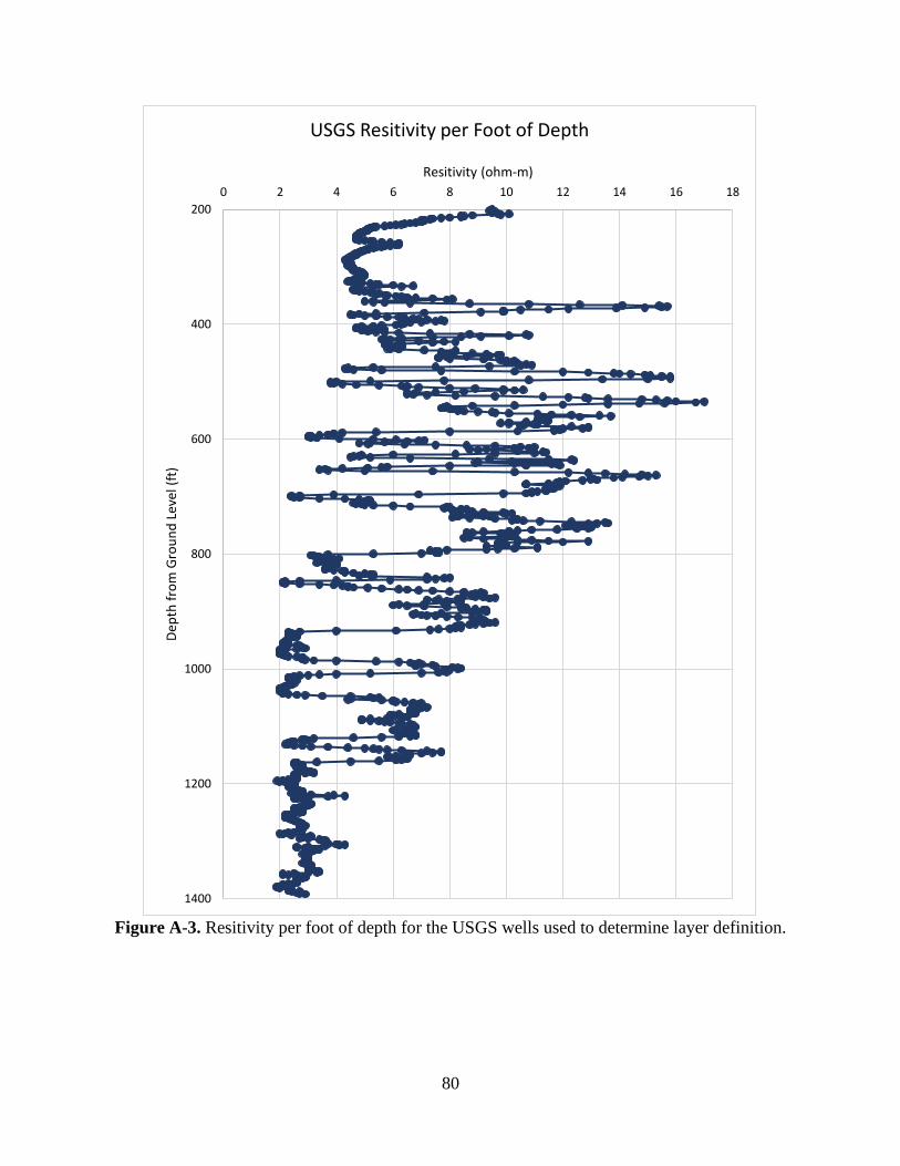
80
Figure A-3. Resitivity per foot of depth for the USGS wells used to determine layer definition.
200
400
600
800
1000
1200
1400
0 2 4 6 8 10 12 14 16 18
Dep
th f
rom
Gro
un
d L
evel
(ft
)Resitivity (ohm-m)
USGS Resitivity per Foot of Depth

81
Figure A-4. Apparent conductance per foot of depth for the USGS wells used to determine layer
definition.
200
400
600
800
1000
1200
1400
0 50 100 150 200 250 300 350 400 450 500
Dep
th f
rom
Gro
un
d L
evel
(ft
)
Apparent Conductance (mmho/m)
USGS Apparent Conductance per Foot of Depth
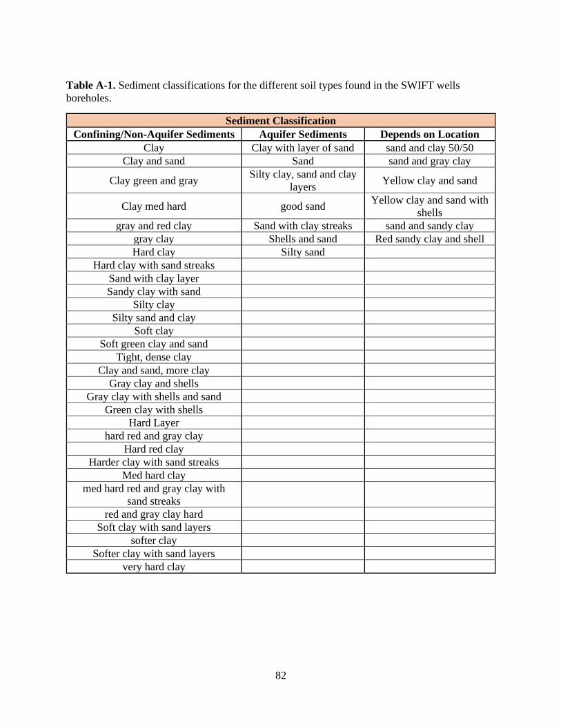
82
Table A-1. Sediment classifications for the different soil types found in the SWIFT wells
boreholes.
Sediment Classification
Confining/Non-Aquifer Sediments Aquifer Sediments Depends on Location
Clay Clay with layer of sand sand and clay 50/50
Clay and sand Sand sand and gray clay
Clay green and gray Silty clay, sand and clay
layers Yellow clay and sand
Clay med hard good sand Yellow clay and sand with
shells
gray and red clay Sand with clay streaks sand and sandy clay
gray clay Shells and sand Red sandy clay and shell
Hard clay Silty sand
Hard clay with sand streaks
Sand with clay layer
Sandy clay with sand
Silty clay
Silty sand and clay
Soft clay
Soft green clay and sand
Tight, dense clay
Clay and sand, more clay
Gray clay and shells
Gray clay with shells and sand
Green clay with shells
Hard Layer
hard red and gray clay
Hard red clay
Harder clay with sand streaks
Med hard clay
med hard red and gray clay with
sand streaks
red and gray clay hard
Soft clay with sand layers
softer clay
Softer clay with sand layers
very hard clay
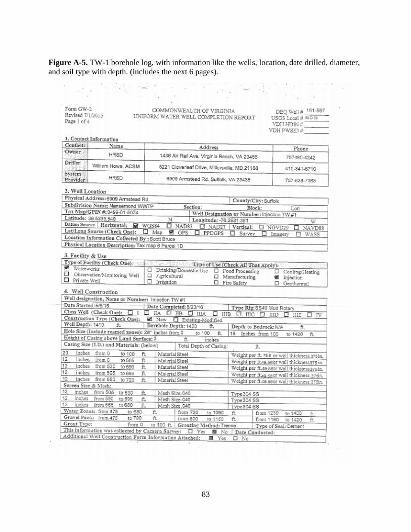
83
Figure A-5. TW-1 borehole log, with information like the wells, location, date drilled, diameter,
and soil type with depth. (includes the next 6 pages).
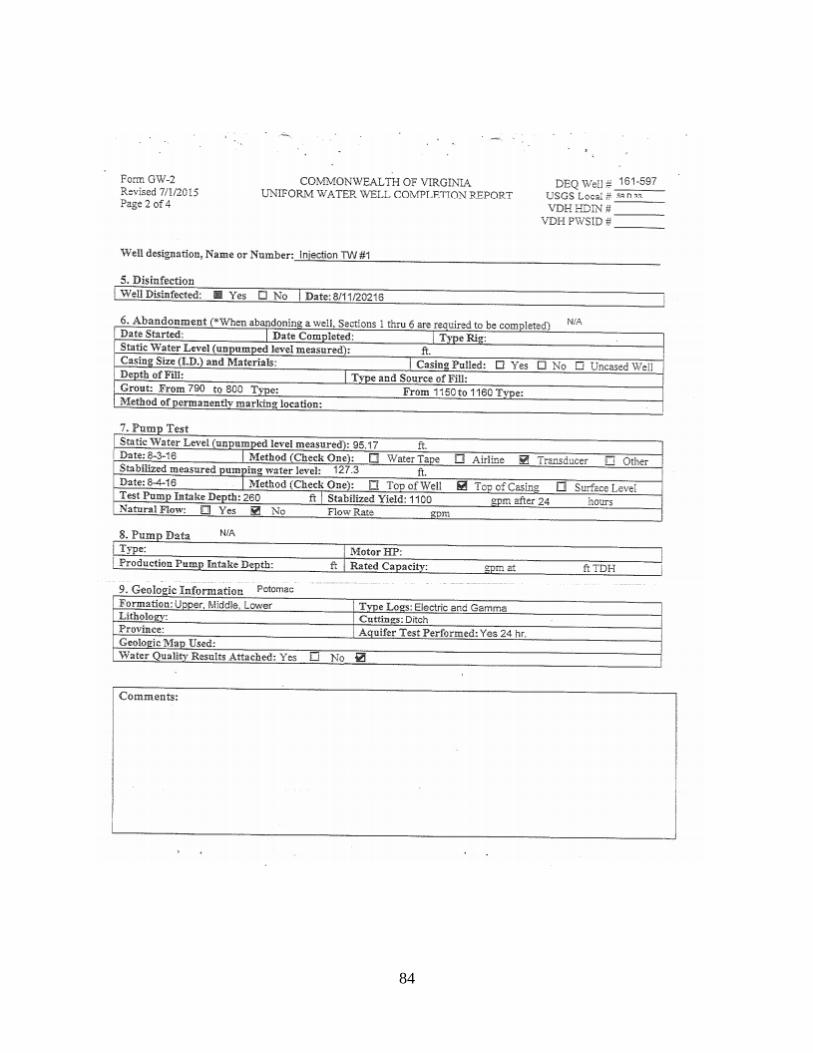
84

85
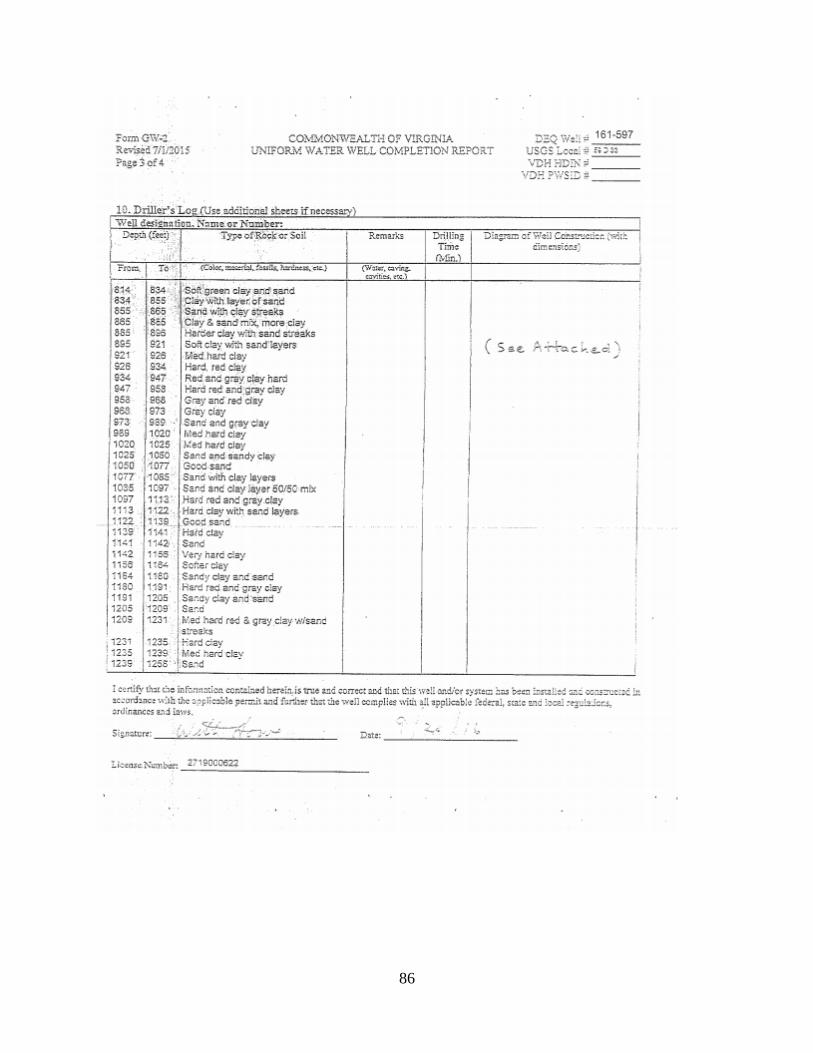
86
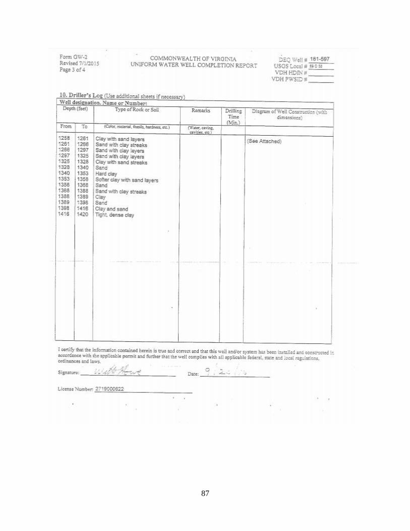
87
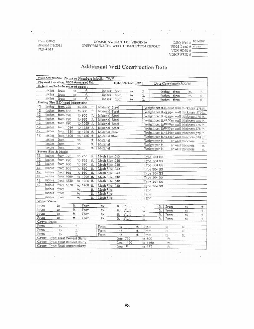
88
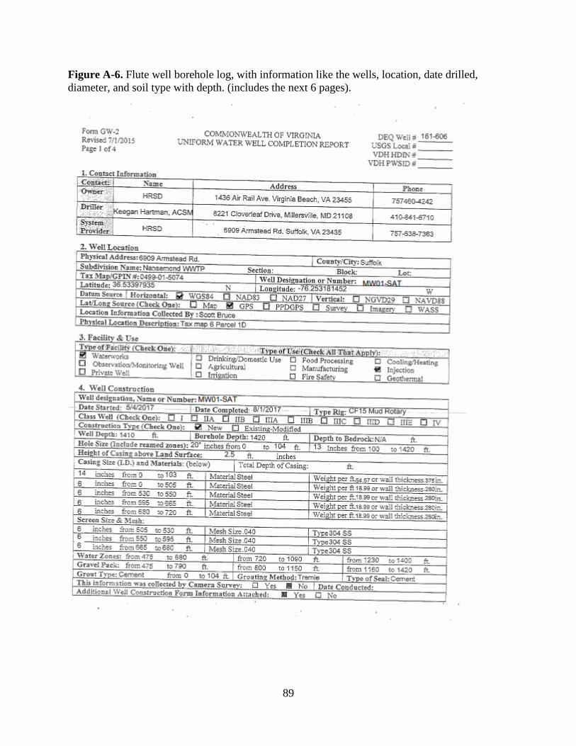
89
Figure A-6. Flute well borehole log, with information like the wells, location, date drilled,
diameter, and soil type with depth. (includes the next 6 pages).
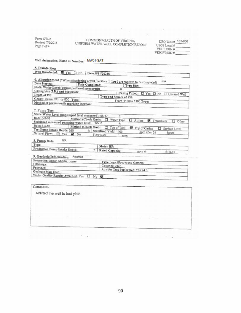
90

91
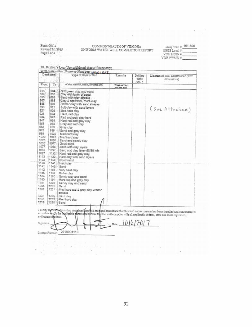
92

93
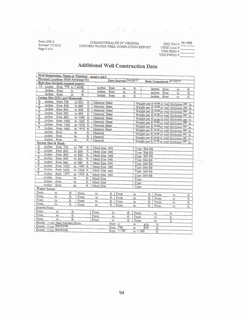
94
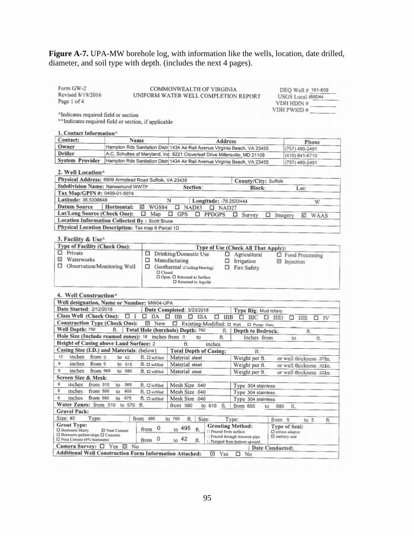
95
Figure A-7. UPA-MW borehole log, with information like the wells, location, date drilled,
diameter, and soil type with depth. (includes the next 4 pages).
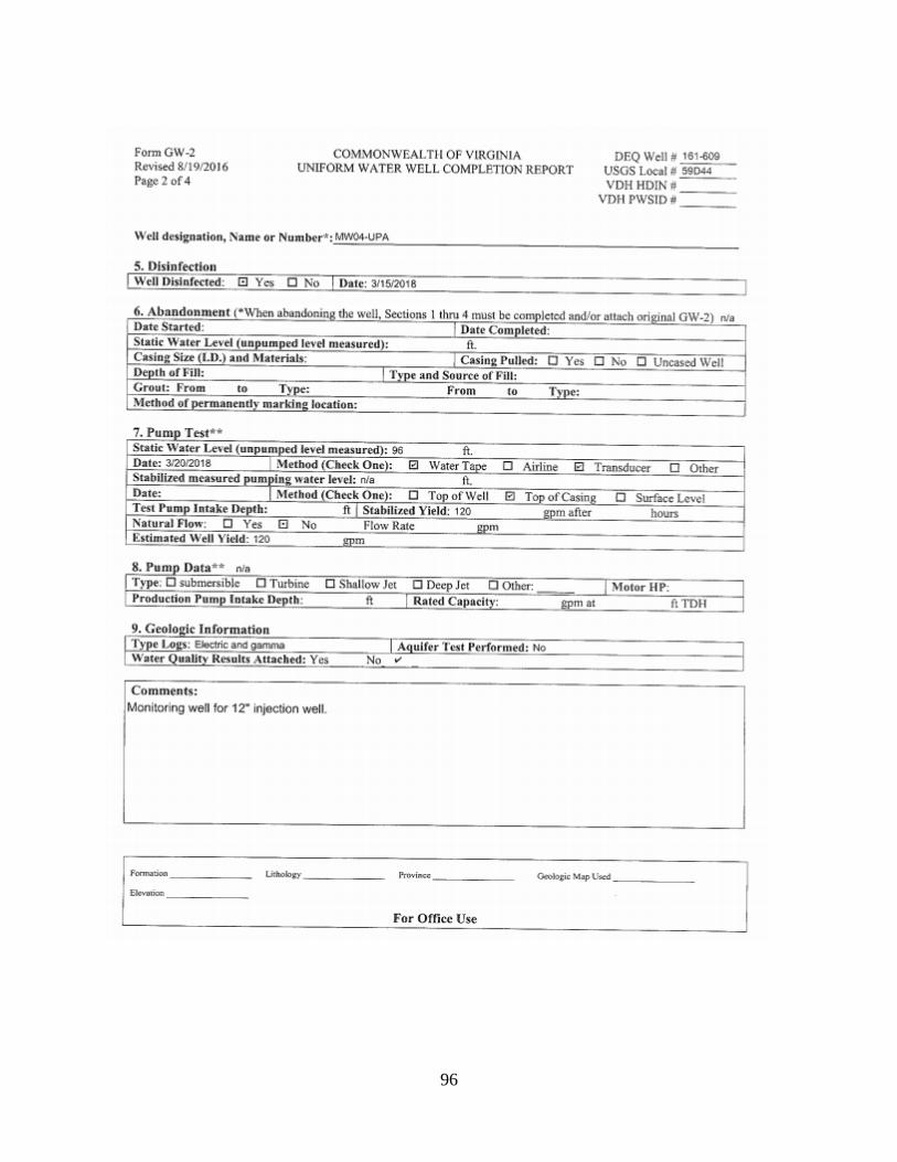
96
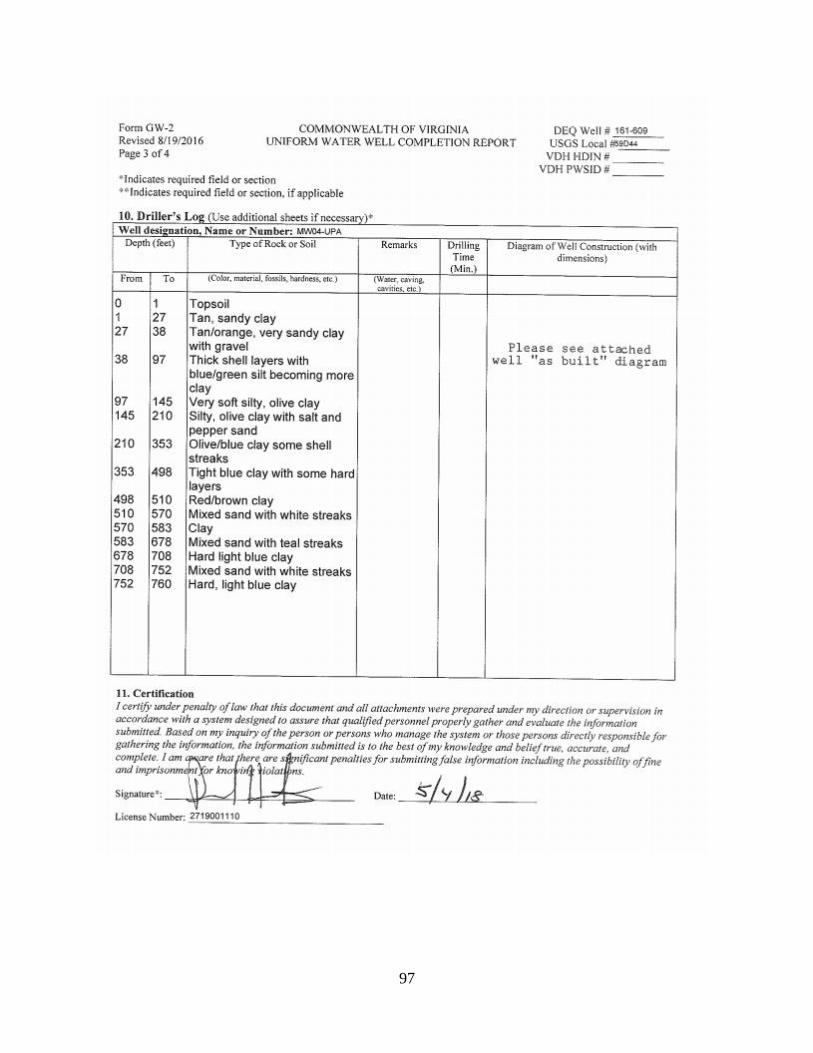
97

98

99
Figure A-8. MPA-MW borehole log, with information like the wells, location, date drilled,
diameter, and soil type with depth. (includes the next 4 pages).
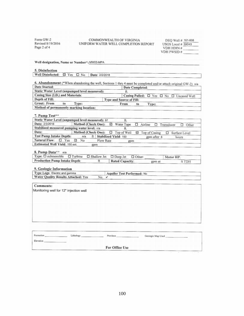
100
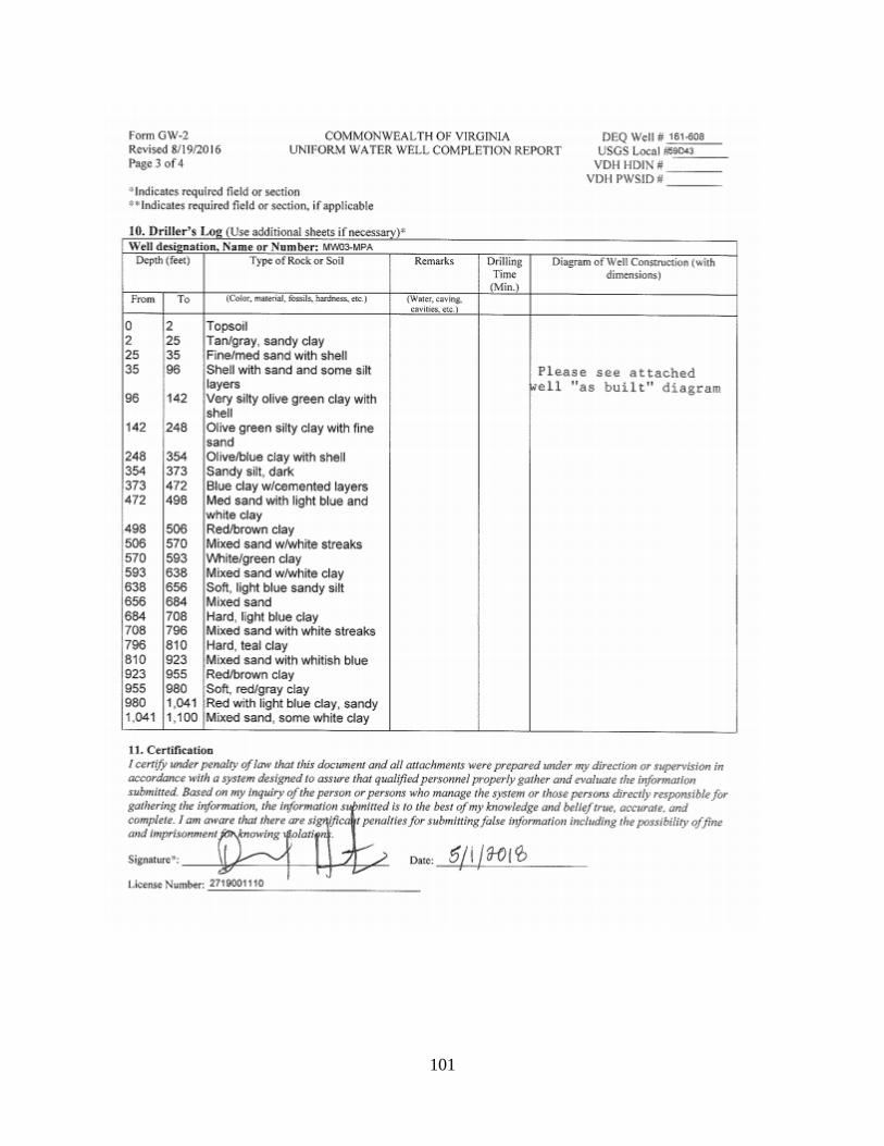
101
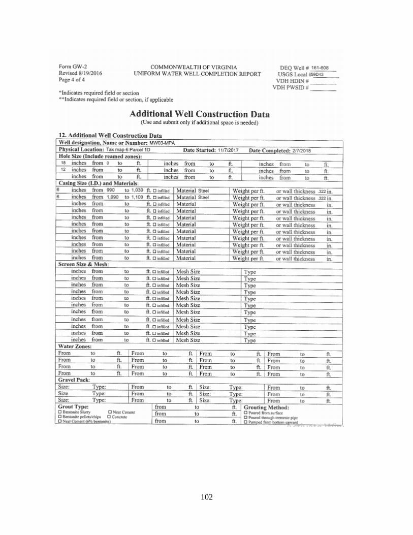
102
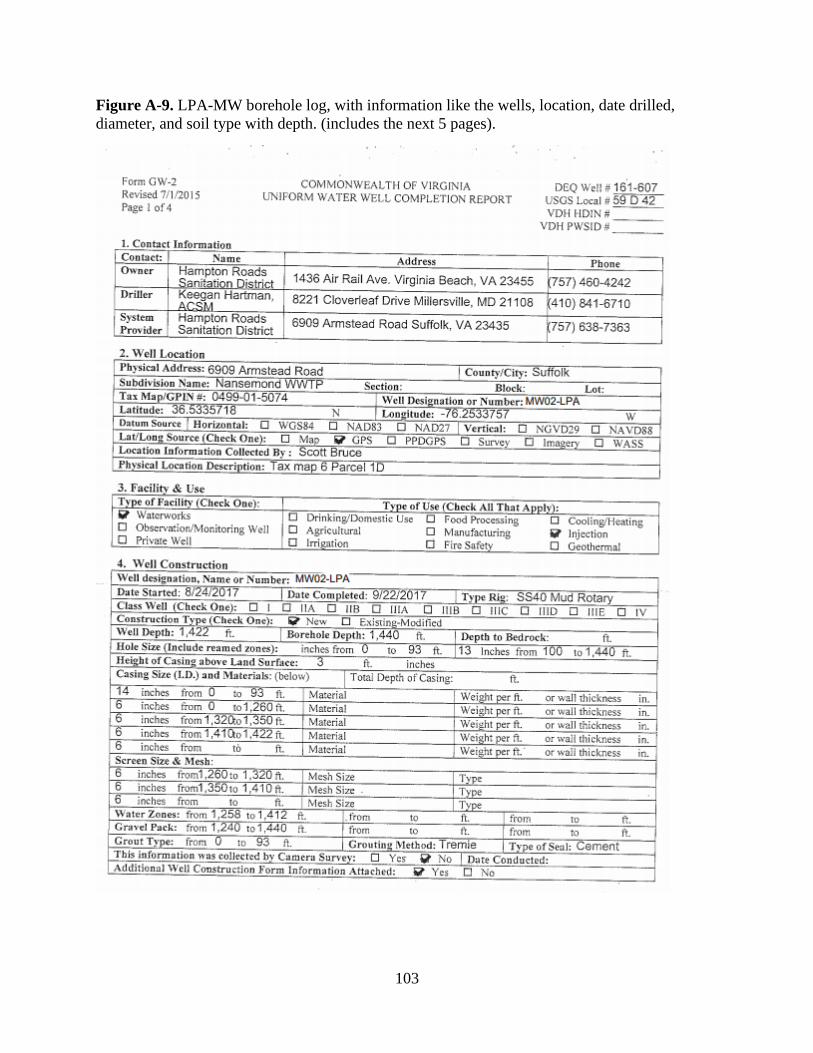
103
Figure A-9. LPA-MW borehole log, with information like the wells, location, date drilled,
diameter, and soil type with depth. (includes the next 5 pages).

104
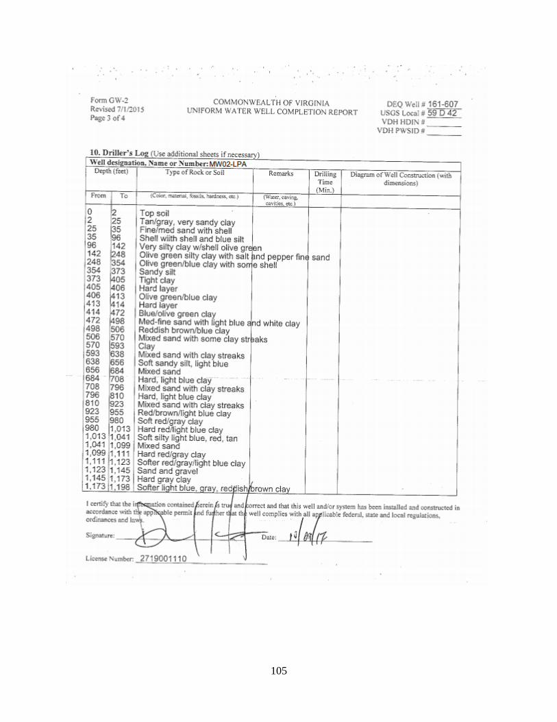
105

106
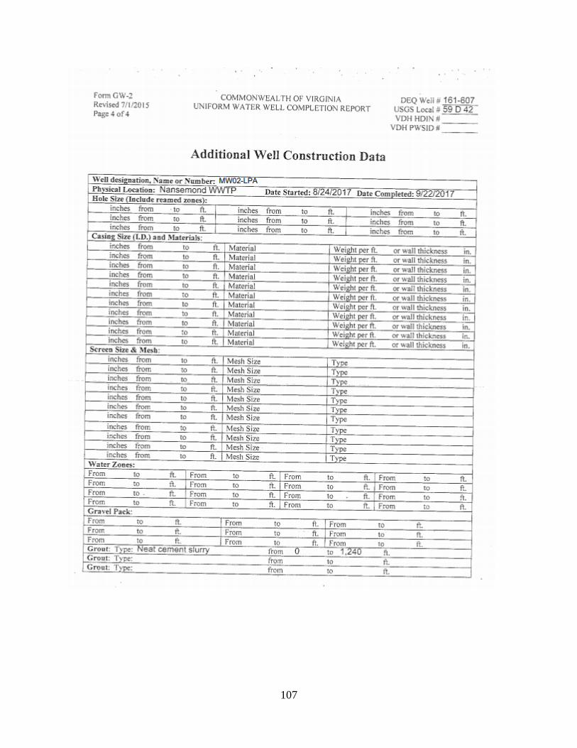
107

108
Figure A-10. Schematic of wells used to determine hydraulic gradient magnitude and direction
with angle and triangle labeled.
Figure A-11. Schematic of right-angle triangle between wells 58C 58 and 59D 36 used in
hydraulic gradient magnitude and direction calculations.

109
Table A-2. Distances between wells used to calculate hydraulic gradient magnitude and
direction.
Line Segment Distance
(ft) Well 1 Well 2
58C 58 59D 25 62210.0
59D 25 59D 36 26144.8
59D 36 59C 31 28820.0
59D 36 58C 58 49959.5
59C 31 58C 58 50655.0
58C 58 RA 13199.8
59D 36 RA 48184.2
Table A-3. Angles of triangles made by the wells used to calculate hydraulic gradient magnitude
and direction.
Angle Degrees
A 74.7
B 72.0
C 33.3
D 23.9
E 50.8
F 105.3
G 15.3

110
Time (min) Drawdown (ft)
1 0.01
2 0.11
3 0.28
4 0.41
5 0.53
6 0.63
7 0.71
8 0.79
9 0.87
10 0.93
11 0.99
12 1.05
13 1.11
14 1.16
15 1.20
16 1.25
17 1.29
18 1.33
36 1.86
54 2.21
72 2.47
108 2.83
144 3.11
180 3.31
216 3.46
252 3.58
288 3.68
360 3.88
432 4.06
504 4.25
576 4.44
648 4.62
720 4.77
792 4.90
864 4.96
936 4.96
1008 4.92
1080 4.92
1152 4.95
1224 4.95
1296 4.99
1440 5.20
8/18 UPA-MW Theis Method
Parameter
Pre-Flow
Rate
Post-Flow
Rate
Q (ft3/min) 86.32 109.25
S (ft) 0.10 0.10
time (min) 10.00 10.00
1/u 4.10 4.10
W(u) 0.12 0.12
R (ft) 340 340
b (ft) 260 260
T (ft2/min) 8.24 10.43
T (ft2/day) 11870 15023
K (ft/day) 45.65 57.78
S 6.96E-04 8.80E-04
Ss (1/ft) 2.68E-06 3.39E-06
8/18 UPA-MW Cooper-Jacob Method
Parameter
Pre-Flow
Rate
Post-Flow
Rate
Q (ft3/min) 86.32 109.25
R (ft) 340 340
b (ft) 260 260
dt 108 108
ds 1.25 1.25
to 4.36 4.36
T (ft2/min) 7.62 9.90
T (ft2/day) 10967 14259
K (ft/day) 42.18 54.84
S 6.47E-04 8.41E-04
Ss (1/ft) 2.49E-06 3.24E-06
Figure A-12. 8/18 UPA-MW: figure contains data set used for Theis and Cooper-Jacob calculations. W(u) vs 1/u overlayer on drawdown vs time graph for Theis method. Drawdown
vs time on a log scale for the Cooper-Jacob method. The Parameters used and results found with the Theis method with the pre and post flow distribution. The Parameters used and
results found with the Cooper-Jacob method with both the pre and post flow distribution. Light green data are the data used for the linear line for the Cooper-Jacob method and the
dark green are the two points used for the Cooper-Jacob calculations.
y = 0.8832ln(x) - 1.3014R² = 0.9996
0
1
2
3
4
5
6
0.1 1 10 100 1000 10000
Dra
wd
ow
n, s (
ft)
Time, t (min)
Cooper-Jacob Method with 8/18 data from the UPA-MW

111
Time (min) Drawdown (ft)
1 0.00
6 0.01
12 0.01
18 0.00
24 0.00
30 0.01
60 0.01
90 0.02
120 0.04
180 0.06
240 0.07
300 0.10
360 0.11
420 0.16
480 0.22
540 0.30
600 0.39
660 0.58
720 0.76
780 0.93
840 1.07
900 1.17
960 1.20
1020 1.18
1080 1.13
1140 1.14
1200 1.25
1260 1.40
1320 1.57
1380 1.72
1440 1.83
8/18 USGS-UPA Cooper-Jacob Method
parameter
Pre-Flow
Rate
Post-Flow
Rate
Q (ft3/min) 86.32 109.25
R (ft) 1270 1270
b (ft) 260 260
dt 360 360
ds 0.81 0.81
to 464.28 464.28
T (ft2/min) 3.99 5.05
T (ft2/day) 5740 7266
K (ft/day) 22.08 27.94
S 2.58E-03 3.27E-03
Ss (1/ft) 9.93E-06 1.26E-05
Figure A-13. 8/18 USGS-UPA: figure contains data set used for Theis and Cooper-Jacob calculations. W(u) vs 1/u overlayer on drawdown vs time graph for Theis method.
Drawdown vs time on a log scale for the Cooper-Jacob method. The Parameters used and results found with the Cooper-Jacob method with both the pre and post flow distribution.
Light green data are the data used for the linear line for the Cooper-Jacob method and the dark green are the two points used for the Cooper-Jacob calculations.
y = 1.7291ln(x) - 10.6169R² = 0.9859
0.0
0.5
1.0
1.5
2.0
0.1 1 10 100 1000 10000
Dra
wd
ow
n, s (
ft)
Time, t (min)
Cooper-Jacob Method with 8/18 data from the USGS-UPA
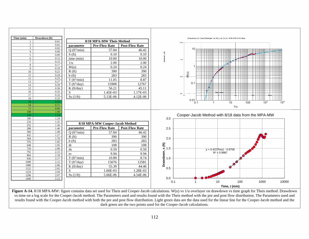
112
Time (min) Drawdown (ft)
1 0.01
2 0.02
3 0.02
4 0.06
5 0.09
6 0.12
7 0.15
8 0.17
9 0.19
10 0.21
11 0.24
12 0.25
13 0.27
14 0.29
15 0.30
16 0.32
17 0.33
18 0.35
36 0.55
54 0.71
72 0.83
108 1.00
144 1.14
180 1.24
216 1.31
252 1.36
288 1.40
360 1.49
432 1.57
504 1.70
576 1.82
648 1.95
720 2.06
792 2.15
864 2.18
936 2.17
1008 2.12
1080 2.06
1152 2.05
1224 2.04
1296 2.07
1440 2.22
8/18 MPA-MW Theis Method
parameter Pre-Flow Rate Post-Flow Rate
Q (ft3/min) 57.84 46.42
S (ft) 0.10 0.10
time (min) 10.00 10.00
1/u 2.00 2.00
W(u) 0.24 0.24
R (ft) 390 390
b (ft) 283 283
T (ft2/min) 11.05 8.87
T (ft2/day) 15908 12767
K (ft/day) 56.21 45.11
S 1.45E-03 1.17E-03
Ss (1/ft) 5.13E-06 4.12E-06
8/18 MPA-MW Cooper-Jacob Method
parameter Pre-Flow Rate Post-Flow Rate
Q (ft3/min) 57.84 46.42
R (ft) 390 390
b (ft) 283 283
dt 108 108
ds 0.59 0.59
to 9.94 9.94
T (ft2/min) 10.89 8.74
T (ft2/day) 15676 12581
K (ft/day) 55.39 44.46
S 1.60E-03 1.28E-03
Ss (1/ft) 5.66E-06 4.54E-06
Figure A-14. 8/18 MPA-MW: figure contains data set used for Theis and Cooper-Jacob calculations. W(u) vs 1/u overlayer on drawdown vs time graph for Theis method. Drawdown
vs time on a log scale for the Cooper-Jacob method. The Parameters used and results found with the Theis method with the pre and post flow distribution. The Parameters used and
results found with the Cooper-Jacob method with both the pre and post flow distribution. Light green data are the data used for the linear line for the Cooper-Jacob method and the
dark green are the two points used for the Cooper-Jacob calculations.
y = 0.4227ln(x) - 0.9708R² = 0.9987
0.0
0.5
1.0
1.5
2.0
2.5
3.0
0.1 1 10 100 1000 10000
Dra
wd
ow
n, s (
ft)
Time, t (min)
Cooper-Jacob Method with 8/18 data from the MPA-MW

113
Time (min) Drawdown (ft)
1 0.00
6 0.00
12 0.02
18 0.04
24 0.11
30 0.24
60 0.30
90 0.35
120 0.43
180 0.49
240 0.51
300 0.54
360 0.56
420 0.59
480 0.64
540 0.70
600 0.76
660 0.91
720 1.06
780 1.19
840 1.29
900 1.34
960 1.32
1020 1.24
1080 1.13
1140 1.07
1200 1.09
1260 1.17
1320 1.27
1380 1.37
1440 1.46
Figure A-15. 8/18 USGS-MPA: figure contains data set used for Theis and Cooper-Jacob calculations. W(u) vs 1/u overlayer on drawdown vs time
graph for Theis method. Drawdown vs time on a log scale for the Cooper-Jacob method. Light green data are the data used for the linear line for the
Cooper-Jacob method.
y = 0.2649ln(x) - 0.8275R² = 0.9993
0.0
0.5
1.0
1.5
2.0
0.1 1 10 100 1000 10000
Dra
wd
ow
n, s (
ft)
Time, t (min)
Cooper-Jacob Method with 8/18 data from the USGS-MPA
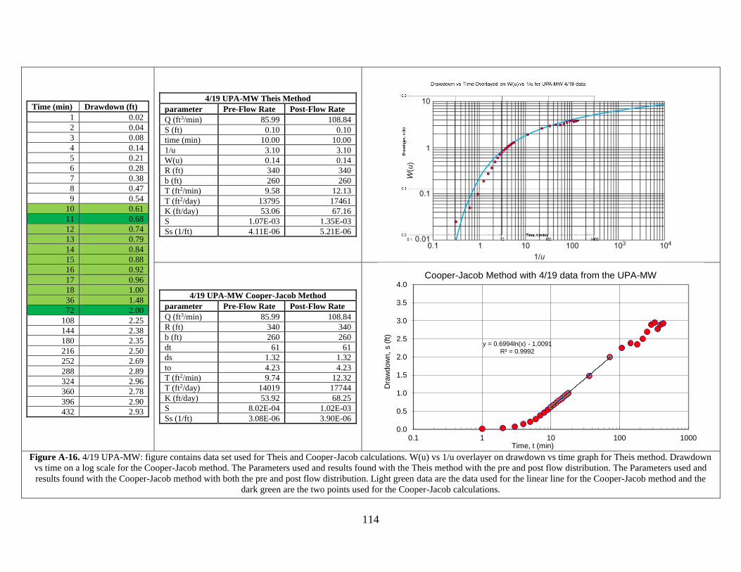
114
Time (min) Drawdown (ft)
1 0.02
2 0.04
3 0.08
4 0.14
5 0.21
6 0.28
7 0.38
8 0.47
9 0.54
10 0.61
11 0.68
12 0.74
13 0.79
14 0.84
15 0.88
16 0.92
17 0.96
18 1.00
36 1.48
72 2.00
108 2.25
144 2.38
180 2.35
216 2.50
252 2.69
288 2.89
324 2.96
360 2.78
396 2.90
432 2.93
4/19 UPA-MW Theis Method
parameter Pre-Flow Rate Post-Flow Rate
Q (ft3/min) 85.99 108.84
S (ft) 0.10 0.10
time (min) 10.00 10.00
1/u 3.10 3.10
W(u) 0.14 0.14
R (ft) 340 340
b (ft) 260 260
T (ft2/min) 9.58 12.13
T (ft2/day) 13795 17461
K (ft/day) 53.06 67.16
S 1.07E-03 1.35E-03
Ss (1/ft) 4.11E-06 5.21E-06
4/19 UPA-MW Cooper-Jacob Method
parameter Pre-Flow Rate Post-Flow Rate
Q (ft3/min) 85.99 108.84
R (ft) 340 340
b (ft) 260 260
dt 61 61
ds 1.32 1.32
to 4.23 4.23
T (ft2/min) 9.74 12.32
T (ft2/day) 14019 17744
K (ft/day) 53.92 68.25
S 8.02E-04 1.02E-03
Ss (1/ft) 3.08E-06 3.90E-06
Figure A-16. 4/19 UPA-MW: figure contains data set used for Theis and Cooper-Jacob calculations. W(u) vs 1/u overlayer on drawdown vs time graph for Theis method. Drawdown
vs time on a log scale for the Cooper-Jacob method. The Parameters used and results found with the Theis method with the pre and post flow distribution. The Parameters used and
results found with the Cooper-Jacob method with both the pre and post flow distribution. Light green data are the data used for the linear line for the Cooper-Jacob method and the
dark green are the two points used for the Cooper-Jacob calculations.
y = 0.6994ln(x) - 1.0091R² = 0.9992
0.0
0.5
1.0
1.5
2.0
2.5
3.0
3.5
4.0
0.1 1 10 100 1000
Dra
wdow
n,
s (
ft)
Time, t (min)
Cooper-Jacob Method with 4/19 data from the UPA-MW

115
Time (min) Drawdown (ft)
1 0.01
6 0.01
12 0.01
18 0.00
24 0.00
30 0.00
42 0.00
54 0.00
66 0.00
78 0.01
90 0.01
102 0.01
114 0.02
126 0.03
138 0.03
150 0.03
162 0.04
174 0.03
186 0.03
198 0.03
210 0.03
222 0.02
240 0.02
252 0.02
264 0.02
276 0.01
288 0.01
300 0.01
312 0.01
324 0.01
336 0.02
348 0.03
360 0.03
372 0.05
384 0.05
396 0.06
408 0.08
420 0.1
432 0.13
444 0.13
456 0.12
Figure A-17. 4/19 USGS-UPA: figure contains data set used for Theis and Cooper-Jacob calculations. W(u) vs 1/u overlayer on drawdown vs time
graph for Theis method. Drawdown vs time on a log scale for the Cooper-Jacob method.
0
0.02
0.04
0.06
0.08
0.1
0.12
0.14
1 10 100 1000
Dra
wd
ow
n (
ft)
Time (min)
Cooper-Jacob Method with 4/19 data from the USGS-UPA

116
Time (min) Drawdown (ft)
1 0.01
2 0.02
3 0.02
4 0.04
5 0.07
6 0.10
7 0.14
8 0.17
9 0.21
10 0.25
11 0.27
12 0.30
13 0.33
14 0.36
15 0.38
16 0.40
17 0.42
18 0.44
36 0.72
72 1.06
108 1.25
144 1.36
180 1.36
216 1.43
252 1.53
288 1.63
324 1.68
360 1.63
396 1.68
432 1.70
8/18 MPA-MW Theis Method
parameter Pre-Flow Rate Post-Flow Rate
Q (ft3/min) 57.62 46.25
S (ft) 0.10 0.10
time (min) 10.00 10.00
1/u 1.80 1.80
W(u) 0.20 0.20
R (ft) 390 390
b (ft) 283 283
T (ft2/min) 9.17 7.36
T (ft2/day) 13206 10599
K (ft/day) 46.67 37.45
S 1.34E-03 1.08E-03
Ss (1/ft) 4.73E-06 3.80E-06
8/18 MPA-MW Cooper-Jacob Method
parameter Pre-Flow Rate Post-Flow Rate
Q (ft3/min) 57.62 46.25
R (ft) 390 390
b (ft) 283 283
dt 90 90
ds 0.81 0.81
to 7.04 7.04
T (ft2/min) 10.14 8.14
T (ft2/day) 14599 11717
K (ft/day) 51.59 41.40
S 1.06E-03 8.48E-04
Ss (1/ft) 3.73E-06 3.00E-06
Figure A-18. 4/19 MPA-MW: figure contains data set used for Theis and Cooper-Jacob calculations. W(u) vs 1/u overlayer on drawdown vs time graph for Theis method. Drawdown
vs time on a log scale for the Cooper-Jacob method. The Parameters used and results found with the Theis method with the pre and post flow distribution. The Parameters used and
results found with the Cooper-Jacob method with both the pre and post flow distribution. Light green data are the data used for the linear line for the Cooper-Jacob method and the
dark green are the two points used for the Cooper-Jacob calculations.
y = 0.4548ln(x) - 0.8879R² = 0.9979
0.0
0.5
1.0
1.5
2.0
0.1 1 10 100 1000
Dra
wdow
n,
s (
ft)
Time, t (min)
Cooper-Jacob Method with 4/19 data from the MPA-MW
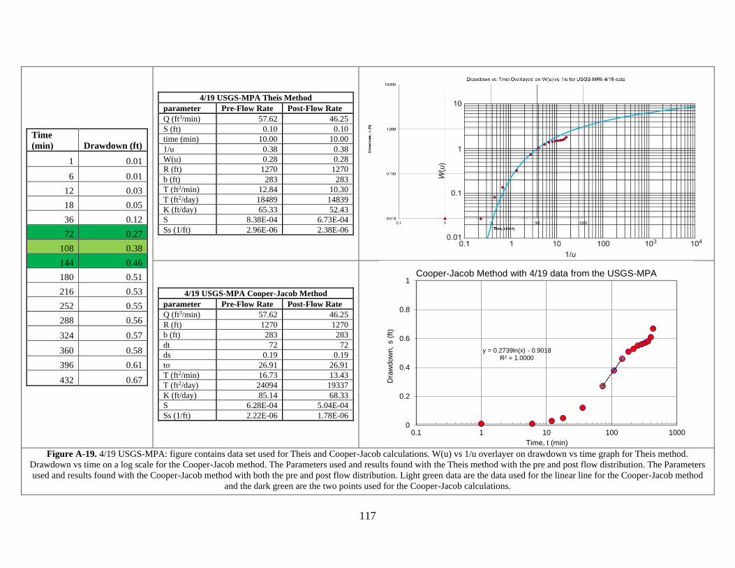
117
Time
(min) Drawdown (ft)
1 0.01
6 0.01
12 0.03
18 0.05
36 0.12
72 0.27
108 0.38
144 0.46
180 0.51
216 0.53
252 0.55
288 0.56
324 0.57
360 0.58
396 0.61
432 0.67
4/19 USGS-MPA Theis Method
parameter Pre-Flow Rate Post-Flow Rate
Q (ft3/min) 57.62 46.25
S (ft) 0.10 0.10
time (min) 10.00 10.00
1/u 0.38 0.38
W(u) 0.28 0.28
R (ft) 1270 1270
b (ft) 283 283
T (ft2/min) 12.84 10.30
T (ft2/day) 18489 14839
K (ft/day) 65.33 52.43
S 8.38E-04 6.73E-04
Ss (1/ft) 2.96E-06 2.38E-06
4/19 USGS-MPA Cooper-Jacob Method
parameter Pre-Flow Rate Post-Flow Rate
Q (ft3/min) 57.62 46.25
R (ft) 1270 1270
b (ft) 283 283
dt 72 72
ds 0.19 0.19
to 26.91 26.91
T (ft2/min) 16.73 13.43
T (ft2/day) 24094 19337
K (ft/day) 85.14 68.33
S 6.28E-04 5.04E-04
Ss (1/ft) 2.22E-06 1.78E-06
Figure A-19. 4/19 USGS-MPA: figure contains data set used for Theis and Cooper-Jacob calculations. W(u) vs 1/u overlayer on drawdown vs time graph for Theis method.
Drawdown vs time on a log scale for the Cooper-Jacob method. The Parameters used and results found with the Theis method with the pre and post flow distribution. The Parameters
used and results found with the Cooper-Jacob method with both the pre and post flow distribution. Light green data are the data used for the linear line for the Cooper-Jacob method
and the dark green are the two points used for the Cooper-Jacob calculations.
y = 0.2739ln(x) - 0.9018R² = 1.0000
0
0.2
0.4
0.6
0.8
1
0.1 1 10 100 1000
Dra
wdow
n,
s (
ft)
Time, t (min)
Cooper-Jacob Method with 4/19 data from the USGS-MPA

118
Table A-4. Layer definition and depth for all 6 wells used in modeling for the low definition
models.
Lower Resolution
Depth from Sea Level (ft) Horizon
Aquifer Classification Testing
Well 1
Flute
Well
UPA
Monitoring
Well
MPA
Monitoring
Well
LPA
Monitoring
Well
USGS
Well
For All
Wells
Non-Aquifer 13.86 13.44 11.45 11.21 10.79 16.68 6
Upper Potomac Confining Unit -386.14 -386.56 -341.55 -361.79 -362.21 -348.32 5
Upper Potomac Aquifer -490.14 -490.56 -498.55 -494.79 -495.21 -480.32 4
Middle Potomac Confining Unit -750.14 -750.56 -740.55 -784.79 -785.21 -727.32 3
Middle Potomac Aquifer -800.14 -800.56 -798.55 -798.79 -799.21 -773.32 2
Lower Potomac Confining Unit -1083.14 -1083.56 -1089.55 -1089.79 -1088.21 -1042.32 1
Lower Potomac Aquifer -1177.14 -1177.56 -1187.55 -1187.79 -1187.21 -1103.32 0
Table A-5. Layer definition and depth for all 6 wells used in modeling for the high definition
multi-layered models.
High Resolution
Depth from Sea Level (ft) Horizon
Aquifer Classification Testing
Well 1
Flute
Well
UPA
Monitoring
Well
MPA
Monitoring
Well
LPA
Monitoring
Well
USGS
Well
For All
Wells
Non-Aquifer 13.86 13.44 11.45 11.21 10.79 16.68 12
Upper Potomac Confining Unit -386.14 -386.56 -341.55 -361.79 -362.21 -348.32 11
Upper Potomac Aquifer Layer 1 -490.14 -490.56 -498.55 -494.79 -495.21 -480.32 10
Upper Confining Unit 1 -523.14 -523.56 -558.55 -558.79 -559.21 -509.32 9
Upper Potomac Aquifer Layer 2 -532.14 -532.56 -571.55 -581.79 -582.21 -525.32 8
Upper Confining Unit 2 -666.14 -666.56 -666.55 -672.79 -673.21 -641.32 7
Upper Potomac Aquifer Layer 3 -677.14 -677.56 -696.55 -696.79 -697.21 -674.32 6
Middle Potomac Confining Unit -750.14 -750.56 -740.55 -784.79 -785.21 -727.32 5
Middle Potomac Aquifer Layer 1 -800.14 -800.56 -798.55 -798.79 -799.21 -772.32 4
Middle Confining Unit 1 -907.14 -907.56 -911.55 -911.79 -912.21 -847.32 3
Middle Potomac Aquifer Layer 2 -959.14 -959.56 -968.55 -968.79 -969.21 -916.32 2
Lower Potomac Confining Unit -1083.14 -1083.56 -1089.55 -1089.79 -1088.21 -1042.32 1
Lower Potomac Aquifer -1177.14 -1177.56 -1187.55 -1187.79 -1187.21 -1103.32 0
Table A-6. GMS Solid unit layers in GMS used for the UPA and MPA single layer models.
GMS Solids Used for Single Layered Models
UPA MPA
GMS Solid layers Horizon Horizon
Non-Aquifer Delete Delete
Upper Potomac Confining Unit Used Delete
Upper Potomac Aquifer Used Delete
Middle Potomac Confining
Unit Used Used
Middle Potomac Aquifer Delete Used
Lower Potomac Confining Unit Delete Used
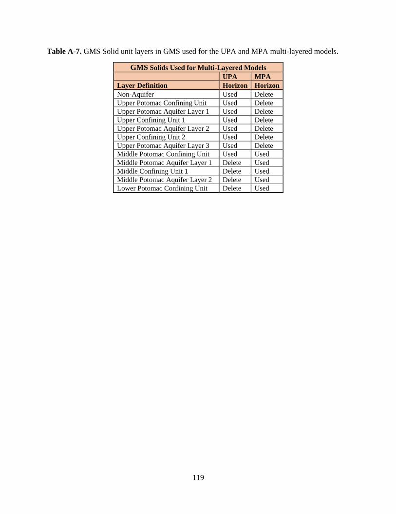
119
Table A-7. GMS Solid unit layers in GMS used for the UPA and MPA multi-layered models.
GMS Solids Used for Multi-Layered Models
UPA MPA
Layer Definition Horizon Horizon
Non-Aquifer Used Delete
Upper Potomac Confining Unit Used Delete
Upper Potomac Aquifer Layer 1 Used Delete
Upper Confining Unit 1 Used Delete
Upper Potomac Aquifer Layer 2 Used Delete
Upper Confining Unit 2 Used Delete
Upper Potomac Aquifer Layer 3 Used Delete
Middle Potomac Confining Unit Used Used
Middle Potomac Aquifer Layer 1 Delete Used
Middle Confining Unit 1 Delete Used
Middle Potomac Aquifer Layer 2 Delete Used
Lower Potomac Confining Unit Delete Used

120
Table A-8. 8/18 and 4/19 data sets used for the SWIFT UPA-MW and USGS-UPA MW
observation points.
UPA Observation Data used for Modeling
8/3/18 UPA-MW 8/3/18 USGA 59D 36 4/26/19 UPA-MW 4/26/19 USGA
Time (days)
Drawdown (ft)
Time (days)
Drawdown (ft)
Time (days)
Drawdown (ft)
Time (days)
Drawdown (ft)
0 -0.207 0 -0.124 0 -0.207 0 -0.124
0.0125 -1.542 0.0125 -0.124 0.0125 -1.205 0.0125 -0.124
0.025 -2.064 0.025 -0.124 0.025 -1.690 0.025 -0.124
0.0375 -2.422 0.05 -0.134 0.05 -2.207 0.05 -0.124
0.05 -2.676 0.0625 -0.134 0.075 -2.459 0.075 -0.144
0.075 -3.042 0.075 -0.144 0.1 -2.587 0.1 -0.164
0.1 -3.315 0.1 -0.164 0.125 -2.559 0.125 -0.154
0.125 -3.516 0.125 -0.184 0.15 -2.710 0.15 -0.144
0.15 -3.664 0.15 -0.194 0.175 -2.899 0.175 -0.144
0.175 -3.788 0.175 -0.224 0.2 -3.101 0.2 -0.134
0.2 -3.891 0.2 -0.234 0.225 -3.164 0.225 -0.134
0.25 -4.085 0.225 -0.284 0.25 -2.984 0.25 -0.154
0.3 -4.266 0.25 -0.344 0.275 -3.102 0.275 -0.184
0.35 -4.460 0.275 -0.424 0.3 -3.135 0.3 -0.254
0.4 -4.647 0.3 -0.514
0.45 -4.822 0.35 -0.704
0.5 -4.976 0.4 -0.884
0.55 -5.107 0.45 -1.054
0.6 -5.168 0.5 -1.194
0.65 -5.168 0.55 -1.294
0.7 -5.132 0.6 -1.324
0.75 -5.132 0.65 -1.304
0.8 -5.152 0.7 -1.254
0.85 -5.157 0.75 -1.264
0.9 -5.201 0.8 -1.374
1 -5.406 0.85 -1.524
0.9 -1.694
0.95 -1.844
1 -1.954
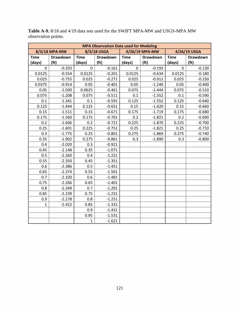
121
Table A-9. 8/18 and 4/19 data sets used for the SWIFT MPA-MW and USGS-MPA MW
observation points.
MPA Observation Data used for Modeling
8/3/18 MPA-MW 8/3/18 USGA 4/26/19 MPA-MW 4/26/19 USGA
Time (days)
Drawdown (ft)
Time (days)
Drawdown (ft)
Time (days)
Drawdown (ft)
Time (days)
Drawdown (ft)
0 -0.203 0 -0.161 0 -0.193 0 -0.130
0.0125 -0.554 0.0125 -0.201 0.0125 -0.634 0.0125 -0.180
0.025 -0.755 0.025 -0.271 0.025 -0.912 0.025 -0.250
0.0375 -0.914 0.05 -0.401 0.05 -1.249 0.05 -0.400
0.05 -1.030 0.0625 -0.461 0.075 -1.444 0.075 -0.510
0.075 -1.208 0.075 -0.511 0.1 -1.552 0.1 -0.590
0.1 -1.341 0.1 -0.591 0.125 -1.552 0.125 -0.640
0.125 -1.444 0.125 -0.651 0.15 -1.620 0.15 -0.660
0.15 -1.511 0.15 -0.671 0.175 -1.719 0.175 -0.680
0.175 -1.560 0.175 -0.701 0.2 -1.821 0.2 -0.690
0.2 -1.606 0.2 -0.721 0.225 -1.870 0.225 -0.700
0.25 -1.691 0.225 -0.751 0.25 -1.821 0.25 -0.710
0.3 -1.775 0.25 -0.801 0.275 -1.869 0.275 -0.740
0.35 -1.902 0.275 -0.861 0.3 -1.890 0.3 -0.800
0.4 -2.020 0.3 -0.921
0.45 -2.148 0.35 -1.071
0.5 -2.260 0.4 -1.221
0.55 -2.350 0.45 -1.351
0.6 -2.386 0.5 -1.451
0.65 -2.374 0.55 -1.501
0.7 -2.320 0.6 -1.481
0.75 -2.266 0.65 -1.401
0.8 -2.249 0.7 -1.291
0.85 -2.239 0.75 -1.231
0.9 -2.278 0.8 -1.251
1 -2.422 0.85 -1.331
0.9 -1.431
0.95 -1.531
1 -1.621
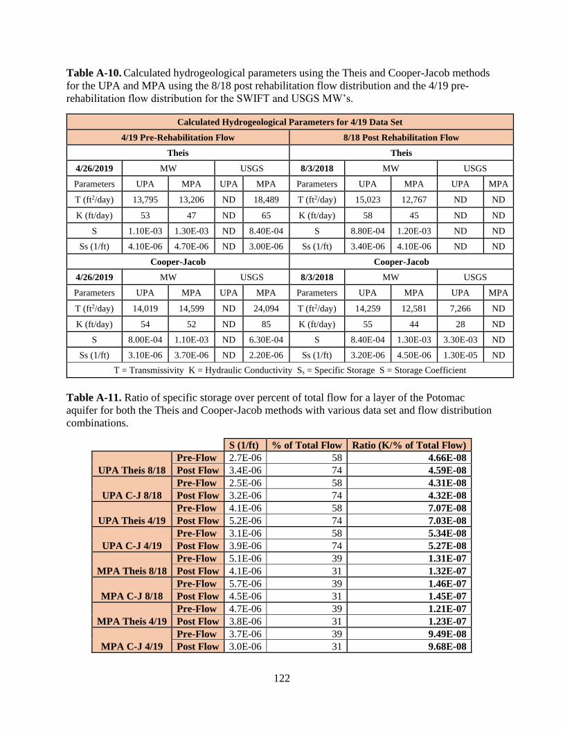
122
Table A-10. Calculated hydrogeological parameters using the Theis and Cooper-Jacob methods
for the UPA and MPA using the 8/18 post rehabilitation flow distribution and the 4/19 pre-
rehabilitation flow distribution for the SWIFT and USGS MW’s.
Calculated Hydrogeological Parameters for 4/19 Data Set
4/19 Pre-Rehabilitation Flow 8/18 Post Rehabilitation Flow
Theis Theis
4/26/2019 MW USGS 8/3/2018 MW USGS
Parameters UPA MPA UPA MPA Parameters UPA MPA UPA MPA
T (ft2/day) 13,795 13,206 ND 18,489 T (ft2/day) 15,023 12,767 ND ND
K (ft/day) 53 47 ND 65 K (ft/day) 58 45 ND ND
S 1.10E-03 1.30E-03 ND 8.40E-04 S 8.80E-04 1.20E-03 ND ND
Ss (1/ft) 4.10E-06 4.70E-06 ND 3.00E-06 Ss (1/ft) 3.40E-06 4.10E-06 ND ND
Cooper-Jacob Cooper-Jacob
4/26/2019 MW USGS 8/3/2018 MW USGS
Parameters UPA MPA UPA MPA Parameters UPA MPA UPA MPA
T (ft2/day) 14,019 14,599 ND 24,094 T (ft2/day) 14,259 12,581 7,266 ND
K (ft/day) 54 52 ND 85 K (ft/day) 55 44 28 ND
S 8.00E-04 1.10E-03 ND 6.30E-04 S 8.40E-04 1.30E-03 3.30E-03 ND
Ss (1/ft) 3.10E-06 3.70E-06 ND 2.20E-06 Ss (1/ft) 3.20E-06 4.50E-06 1.30E-05 ND
T = Transmissivity K = Hydraulic Conductivity Ss = Specific Storage S = Storage Coefficient
Table A-11. Ratio of specific storage over percent of total flow for a layer of the Potomac
aquifer for both the Theis and Cooper-Jacob methods with various data set and flow distribution
combinations.
S (1/ft) % of Total Flow Ratio (K/% of Total Flow)
UPA Theis 8/18
Pre-Flow 2.7E-06 58 4.66E-08
Post Flow 3.4E-06 74 4.59E-08
UPA C-J 8/18
Pre-Flow 2.5E-06 58 4.31E-08
Post Flow 3.2E-06 74 4.32E-08
UPA Theis 4/19
Pre-Flow 4.1E-06 58 7.07E-08
Post Flow 5.2E-06 74 7.03E-08
UPA C-J 4/19
Pre-Flow 3.1E-06 58 5.34E-08
Post Flow 3.9E-06 74 5.27E-08
MPA Theis 8/18
Pre-Flow 5.1E-06 39 1.31E-07
Post Flow 4.1E-06 31 1.32E-07
MPA C-J 8/18
Pre-Flow 5.7E-06 39 1.46E-07
Post Flow 4.5E-06 31 1.45E-07
MPA Theis 4/19
Pre-Flow 4.7E-06 39 1.21E-07
Post Flow 3.8E-06 31 1.23E-07
MPA C-J 4/19
Pre-Flow 3.7E-06 39 9.49E-08
Post Flow 3.0E-06 31 9.68E-08

123
Figure A-20. Sensitivity of the estimated parameters
within the 8/18 post flow UPA single layer model
using PEST.
Figure A-21. Sensitivity of the estimated parameters
within the 4/19 pre-flow UPA single layer model
using PEST.
Figure A-22. Sensitivity of the estimated parameters
within the 4/19 post flow UPA single layer model
using PEST.
Figure A-23. Sensitivity of the estimated parameters
within the 8/18 post flow MPA single layer model
using PEST.
Figure A-24. Sensitivity of the estimated parameters
within the 4/19 pre-flow MPA single layer model
using PEST.
8.85E-02
2.29E-02
3.93E-05
0.0E+00
1.0E-02
2.0E-02
3.0E-02
4.0E-02
5.0E-02
6.0E-02
7.0E-02
8.0E-02
9.0E-02
1.0E-01
Hydraulic Conductivity(ft/Day)
Specific Storage (1/ft) Conductance(ft^2/Day)/(ft)
Sen
siti
vity
Sensitivity of UPA 8/18 Data Modeled with Post Rehab Flow Rate
3.46E-02
9.99E-03
1.12E-05
0.0E+00
5.0E-03
1.0E-02
1.5E-02
2.0E-02
2.5E-02
3.0E-02
3.5E-02
4.0E-02
Hydraulic Conductivity(ft/Day)
Specific Storage (1/ft) Conductance(ft^2/Day)/(ft)
Sen
siti
vity
Sensitivity of UPA 4/19 Data Modeled with Pre-rehab Flow Rate
3.46E-02
9.99E-03
1.58E-05
0.0E+00
5.0E-03
1.0E-02
1.5E-02
2.0E-02
2.5E-02
3.0E-02
3.5E-02
4.0E-02
Hydraulic Conductivity(ft/Day)
Specific Storage (1/ft) Conductance(ft^2/Day)/(ft)
Sen
siti
vity
Sensitivity of UPA 4/19 Data Modeled with Post Rehab Flow Rate
2.40E-02
1.21E-021.10E-02
0.0E+00
5.0E-03
1.0E-02
1.5E-02
2.0E-02
2.5E-02
3.0E-02
Hydraulic Conductivity(ft/Day)
Specific Storage (1/ft) Conductance(ft^2/Day)/(ft)
Sen
siti
vity
Sensitivity of MPA 8/18 Data Modeled with Post Rehab Flow Rate
1.79E-02
6.16E-03
1.63E-03
0.0E+00
2.0E-03
4.0E-03
6.0E-03
8.0E-03
1.0E-02
1.2E-02
1.4E-02
1.6E-02
1.8E-02
2.0E-02
Hydraulic Conductivity(ft/Day)
Specific Storage (1/ft) Conductance(ft^2/Day)/(ft)
Sen
siti
vity
Sensitivity of MPA 4/19 Data Modeled with Pre-rehab Flow Rate
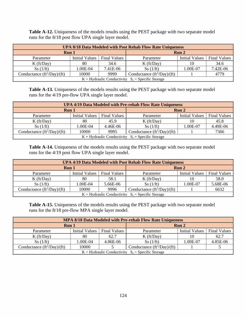
124
Table A-12. Uniqueness of the models results using the PEST package with two separate model
runs for the 8/18 post flow UPA single layer model.
UPA 8/18 Data Modeled with Post Rehab Flow Rate Uniqueness
Run 1 Run 2
Parameter Initial Values Final Values Parameter Initial Values Final Values
K (ft/Day) 80 34.6 K (ft/Day) 10 34.6
Ss (1/ft) 1.00E-04 7.41E-06 Ss (1/ft) 1.00E-07 7.42E-06
Conductance (ft2/Day)/(ft) 10000 9999 Conductance (ft2/Day)/(ft) 1 4779 K = Hydraulic Conductivity Ss = Specific Storage
Table A-13. Uniqueness of the models results using the PEST package with two separate model
runs for the 4/19 pre-flow UPA single layer model.
UPA 4/19 Data Modeled with Pre-rehab Flow Rate Uniqueness
Run 1 Run 2
Parameter Initial Values Final Values Parameter Initial Values Final Values
K (ft/Day) 80 45.9 K (ft/Day) 10 45.8
Ss (1/ft) 1.00E-04 4.46E-06 Ss (1/ft) 1.00E-07 4.49E-06
Conductance (ft2/Day)/(ft) 10000 9995 Conductance (ft2/Day)/(ft) 1 7366 K = Hydraulic Conductivity Ss = Specific Storage
Table A-14. Uniqueness of the models results using the PEST package with two separate model
runs for the 4/19 post flow UPA single layer model.
UPA 4/19 Data Modeled with Post Rehab Flow Rate Uniqueness
Run 1 Run 2
Parameter Initial Values Final Values Parameter Initial Values Final Values
K (ft/Day) 80 58.1 K (ft/Day) 10 58.0
Ss (1/ft) 1.00E-04 5.66E-06 Ss (1/ft) 1.00E-07 5.68E-06
Conductance (ft2/Day)/(ft) 10000 9996 Conductance (ft2/Day)/(ft) 1 6632 K = Hydraulic Conductivity Ss = Specific Storage
Table A-15. Uniqueness of the models results using the PEST package with two separate model
runs for the 8/18 pre-flow MPA single layer model.
MPA 8/18 Data Modeled with Pre-rehab Flow Rate Uniqueness
Run 1 Run 2
Parameter Initial Values Final Values Parameter Initial Values Final Values
K (ft/Day) 80 62.7 K (ft/Day) 10 62.7
Ss (1/ft) 1.00E-04 4.86E-06 Ss (1/ft) 1.00E-07 4.85E-06
Conductance (ft2/Day)/(ft) 10000 5 Conductance (ft2/Day)/(ft) 1 5 K = Hydraulic Conductivity Ss = Specific Storage

125
Table A-16. Uniqueness of the models results using the PEST package with two separate model
runs for the 8/18 post flow MPA single layer model.
MPA 8/18 Data Modeled with Post Rehab Flow Rate Uniqueness
Run 1 Run 2
Parameter Initial Values Final Values Parameter Initial Values Final Values
K (ft/Day) 80 50.2 K (ft/Day) 10 50.3
Ss (1/ft) 1.00E-04 3.90E-06 Ss (1/ft) 1.00E-07 3.90E-06
Conductance (ft2/Day)/(ft) 10000 4 Conductance (ft2/Day)/(ft) 1 4 K = Hydraulic Conductivity Ss = Specific Storage
Table A-17. Uniqueness of the models results using the PEST package with two separate model
runs for the 4/19 pre-flow MPA single layer model.
MPA 4/19 Data Modeled with Pre-rehab Flow Rate Uniqueness
Run 1 Run 2
Parameter Initial Values Final Values Parameter Initial Values Final Values
K (ft/Day) 80 52.5 K (ft/Day) 10 52.4
Ss (1/ft) 1.00E-04 3.77E-06 Ss (1/ft) 1.00E-07 3.78E-06
Conductance (ft2/Day)/(ft) 10000 26 Conductance (ft2/Day)/(ft) 1 26 K = Hydraulic Conductivity Ss = Specific Storage
Table A-18. Uniqueness of the models results using the PEST package with two separate model
runs for the 4/19 post flow MPA single layer model.
MPA 4/19 Data Modeled with Post Rehab Flow Rate Uniqueness
Run 1 Run 2
Parameter Initial Values Final Values Parameter Initial Values Final Values
K (ft/Day) 80 42.1 K (ft/Day) 10 42.1
Ss (1/ft) 1.00E-04 3.03E-06 Ss (1/ft) 1.00E-07 3.03E-06
Conductance (ft2/Day)/(ft) 5000 21 Conductance (ft2/Day)/(ft) 1 21 K = Hydraulic Conductivity Ss = Specific Storage
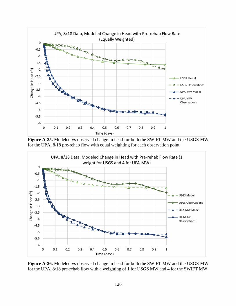
126
Figure A-25. Modeled vs observed change in head for both the SWIFT MW and the USGS MW
for the UPA, 8/18 pre-rehab flow with equal weighting for each observation point.
Figure A-26. Modeled vs observed change in head for both the SWIFT MW and the USGS MW
for the UPA, 8/18 pre-rehab flow with a weighting of 1 for USGS MW and 4 for the SWIFT MW.
-6
-5.5
-5
-4.5
-4
-3.5
-3
-2.5
-2
-1.5
-1
-0.5
0
0 0.1 0.2 0.3 0.4 0.5 0.6 0.7 0.8 0.9 1
Ch
ange
in H
ead
(ft
)
Time (days)
UPA, 8/18 Data, Modeled Change in Head with Pre-rehab Flow Rate (Equally Weighted)
USGS Model
USGS Observations
UPA-MW Model
UPA-MWObservations
-6
-5.5
-5
-4.5
-4
-3.5
-3
-2.5
-2
-1.5
-1
-0.5
0
0 0.1 0.2 0.3 0.4 0.5 0.6 0.7 0.8 0.9 1
Ch
ange
in H
ead
(ft
)
Time (days)
UPA, 8/18 Data, Modeled Change in Head with Pre-rehab Flow Rate (1 weight for USGS and 4 for UPA-MW)
USGS Model
USGS Observations
UPA-MW Model
UPA-MWObservations

127
Figure A-27. Modeled vs observed change in head for both the SWIFT MW and the USGS MW
for the UPA, 8/18 pre-rehab flow with a weighting of 1 for the SWIFT MW and no SWIFT MW.
Figure A-28. Modeled vs observed change in head for both the SWIFT MW and the USGS MW
for the UPA, 8/18 post rehab flow with equal weighting for each observation point.
-6
-5.5
-5
-4.5
-4
-3.5
-3
-2.5
-2
-1.5
-1
-0.5
0
0 0.1 0.2 0.3 0.4 0.5 0.6 0.7 0.8 0.9 1
Ch
ange
in H
ead
(ft
)
Time (days)
UPA, 8/18 Data, Modeled Change in Head with Pre-rehab Flow Rate (0 weight for USGS and 1 for UPA-MW)
UPA-MWModel
UPA-MWObservations
-6
-5.5
-5
-4.5
-4
-3.5
-3
-2.5
-2
-1.5
-1
-0.5
0
0 0.1 0.2 0.3 0.4 0.5 0.6 0.7 0.8 0.9 1
Ch
ange
in H
ead
(ft
)
Time (days)
UPA, 8/18 Data, Modeled Change in Head with Post Rehab Flow Rate (Equally Weighted)
USGS Model
USGS Observations
UPA-MW Model
UPA-MWObservations
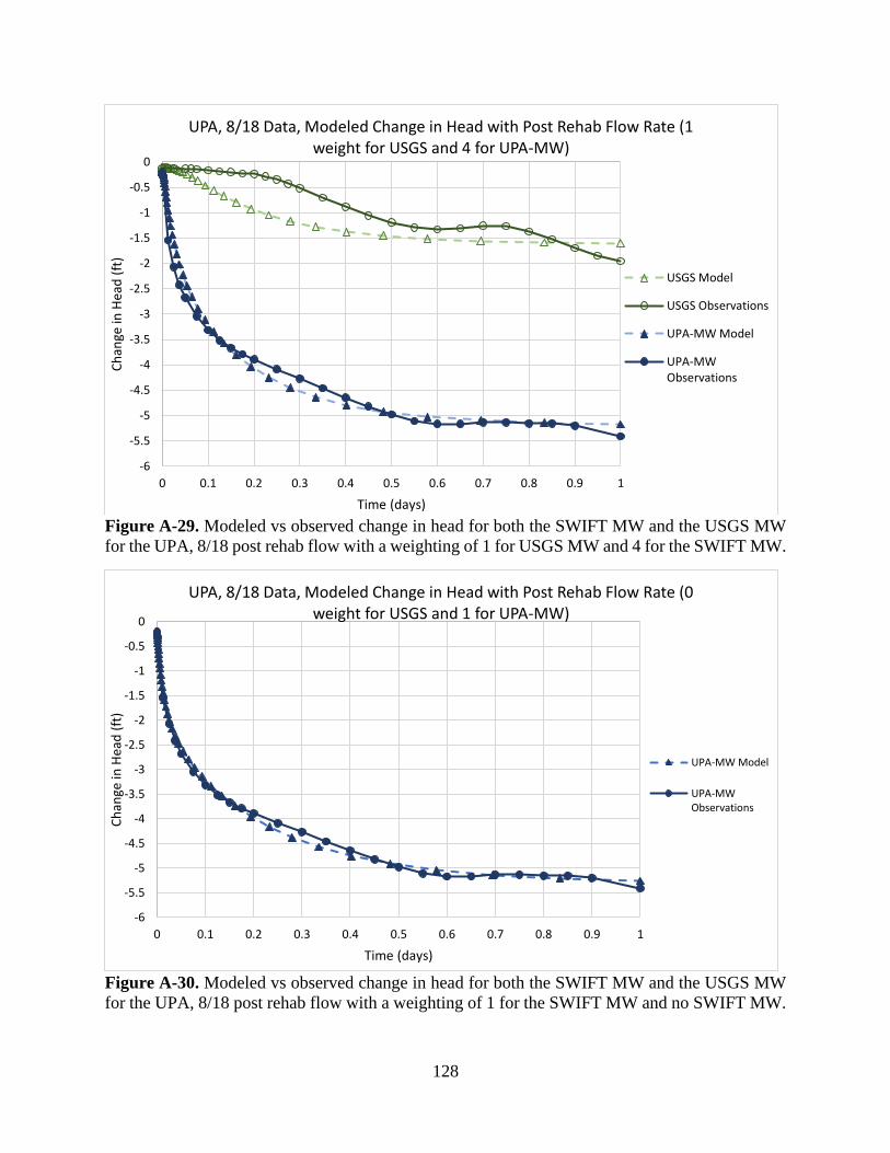
128
Figure A-29. Modeled vs observed change in head for both the SWIFT MW and the USGS MW
for the UPA, 8/18 post rehab flow with a weighting of 1 for USGS MW and 4 for the SWIFT MW.
Figure A-30. Modeled vs observed change in head for both the SWIFT MW and the USGS MW
for the UPA, 8/18 post rehab flow with a weighting of 1 for the SWIFT MW and no SWIFT MW.
-6
-5.5
-5
-4.5
-4
-3.5
-3
-2.5
-2
-1.5
-1
-0.5
0
0 0.1 0.2 0.3 0.4 0.5 0.6 0.7 0.8 0.9 1
Ch
ange
in H
ead
(ft
)
Time (days)
UPA, 8/18 Data, Modeled Change in Head with Post Rehab Flow Rate (1 weight for USGS and 4 for UPA-MW)
USGS Model
USGS Observations
UPA-MW Model
UPA-MWObservations
-6
-5.5
-5
-4.5
-4
-3.5
-3
-2.5
-2
-1.5
-1
-0.5
0
0 0.1 0.2 0.3 0.4 0.5 0.6 0.7 0.8 0.9 1
Ch
ange
in H
ead
(ft
)
Time (days)
UPA, 8/18 Data, Modeled Change in Head with Post Rehab Flow Rate (0 weight for USGS and 1 for UPA-MW)
UPA-MW Model
UPA-MWObservations
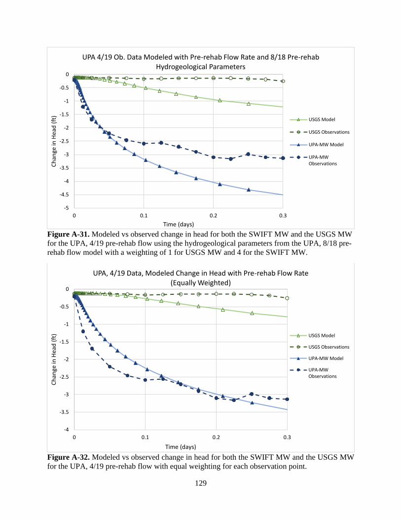
129
Figure A-31. Modeled vs observed change in head for both the SWIFT MW and the USGS MW
for the UPA, 4/19 pre-rehab flow using the hydrogeological parameters from the UPA, 8/18 pre-
rehab flow model with a weighting of 1 for USGS MW and 4 for the SWIFT MW.
Figure A-32. Modeled vs observed change in head for both the SWIFT MW and the USGS MW
for the UPA, 4/19 pre-rehab flow with equal weighting for each observation point.
-5
-4.5
-4
-3.5
-3
-2.5
-2
-1.5
-1
-0.5
0
0 0.1 0.2 0.3
Ch
ange
in H
ead
(ft
)
Time (days)
UPA 4/19 Ob. Data Modeled with Pre-rehab Flow Rate and 8/18 Pre-rehab Hydrogeological Parameters
USGS Model
USGS Observations
UPA-MW Model
UPA-MWObservations
-4
-3.5
-3
-2.5
-2
-1.5
-1
-0.5
0
0 0.1 0.2 0.3
Ch
ange
in H
ead
(ft
)
Time (days)
UPA, 4/19 Data, Modeled Change in Head with Pre-rehab Flow Rate (Equally Weighted)
USGS Model
USGS Observations
UPA-MW Model
UPA-MWObservations
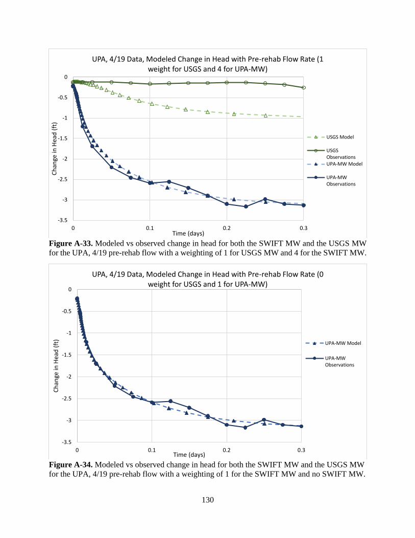
130
Figure A-33. Modeled vs observed change in head for both the SWIFT MW and the USGS MW
for the UPA, 4/19 pre-rehab flow with a weighting of 1 for USGS MW and 4 for the SWIFT MW.
Figure A-34. Modeled vs observed change in head for both the SWIFT MW and the USGS MW
for the UPA, 4/19 pre-rehab flow with a weighting of 1 for the SWIFT MW and no SWIFT MW.
-3.5
-3
-2.5
-2
-1.5
-1
-0.5
0
0 0.1 0.2 0.3
Ch
ange
in H
ead
(ft
)
Time (days)
UPA, 4/19 Data, Modeled Change in Head with Pre-rehab Flow Rate (1 weight for USGS and 4 for UPA-MW)
USGS Model
USGSObservationsUPA-MW Model
UPA-MWObservations
-3.5
-3
-2.5
-2
-1.5
-1
-0.5
0
0 0.1 0.2 0.3
Ch
ange
in H
ead
(ft
)
Time (days)
UPA, 4/19 Data, Modeled Change in Head with Pre-rehab Flow Rate (0 weight for USGS and 1 for UPA-MW)
UPA-MW Model
UPA-MWObservations
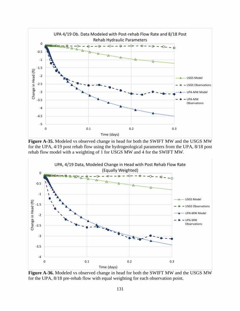
131
Figure A-35. Modeled vs observed change in head for both the SWIFT MW and the USGS MW
for the UPA, 4/19 post rehab flow using the hydrogeological parameters from the UPA, 8/18 post
rehab flow model with a weighting of 1 for USGS MW and 4 for the SWIFT MW.
Figure A-36. Modeled vs observed change in head for both the SWIFT MW and the USGS MW
for the UPA, 8/18 pre-rehab flow with equal weighting for each observation point.
-5
-4.5
-4
-3.5
-3
-2.5
-2
-1.5
-1
-0.5
0
0 0.1 0.2 0.3
Ch
ange
in H
ead
(ft
)
Time (days)
UPA 4/19 Ob. Data Modeled with Post-rehab Flow Rate and 8/18 Post Rehab Hydraulic Parameters
USGS Model
USGS Observations
UPA-MW Model
UPA-MWObservations
-4
-3.5
-3
-2.5
-2
-1.5
-1
-0.5
0
0 0.1 0.2 0.3
Ch
ange
in H
ead
(ft
)
Time (days)
UPA, 4/19 Data, Modeled Change in Head with Post Rehab Flow Rate (Equally Weighted)
USGS Model
USGS Observations
UPA-MW Model
UPA-MWObservations

132
Figure A-37. Modeled vs observed change in head for both the SWIFT MW and the USGS MW
for the UPA, 4/19 post rehab flow with a weighting of 1 for USGS MW and 4 for the SWIFT MW.
Figure A-38. Modeled vs observed change in head for both the SWIFT MW and the USGS MW
for the UPA, 4/19 post rehab flow with a weighting of 1 for the SWIFT MW and no SWIFT MW.
-3.5
-3
-2.5
-2
-1.5
-1
-0.5
0
0 0.1 0.2 0.3
Ch
ange
in H
ead
(ft
)
Time (days)
UPA, 4/19 Data, Modeled Change in Head with Post Rehab Flow Rate (1 weight for USGS and 4 for UPA-MW)
USGS Model
USGS Observations
UPA-MW Model
UPA-MWObservations
-3.5
-3
-2.5
-2
-1.5
-1
-0.5
0
0 0.1 0.2 0.3
Ch
ange
in H
ead
(ft
)
Time (days)
UPA, 4/19 Data, Modeled Change in Head with Post Rehab Flow Rate (0 weight for USGS and 1 for UPA-MW)
UPA-MW Model
UPA-MWObservations
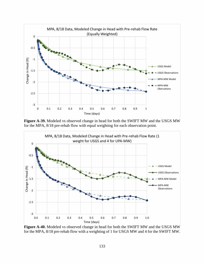
133
Figure A-39. Modeled vs observed change in head for both the SWIFT MW and the USGS MW
for the MPA, 8/18 pre-rehab flow with equal weighting for each observation point.
Figure A-40. Modeled vs observed change in head for both the SWIFT MW and the USGS MW
for the MPA, 8/18 pre-rehab flow with a weighting of 1 for USGS MW and 4 for the SWIFT MW.
-3
-2.5
-2
-1.5
-1
-0.5
0
0 0.1 0.2 0.3 0.4 0.5 0.6 0.7 0.8 0.9 1
Ch
ange
in H
ead
(ft
)
Time (days)
MPA, 8/18 Data, Modeled Change in Head with Pre-rehab Flow Rate (Equally Weighted)
USGS Model
USGS Observations
MPA-MW Model
MPA-MWObervations
-3
-2.5
-2
-1.5
-1
-0.5
0
0.0 0.1 0.2 0.3 0.4 0.5 0.6 0.7 0.8 0.9 1.0
Ch
ange
in H
ead
(ft
)
Time (days)
MPA, 8/18 Data, Modeled Change in Head with Pre-rehab Flow Rate (1 weight for USGS and 4 for UPA-MW)
USGS Model
USGS Observations
MPA-MW Model
MPA-MWObservations
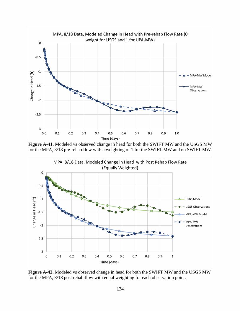
134
Figure A-41. Modeled vs observed change in head for both the SWIFT MW and the USGS MW
for the MPA, 8/18 pre-rehab flow with a weighting of 1 for the SWIFT MW and no SWIFT MW.
Figure A-42. Modeled vs observed change in head for both the SWIFT MW and the USGS MW
for the MPA, 8/18 post rehab flow with equal weighting for each observation point.
-3
-2.5
-2
-1.5
-1
-0.5
0
0.0 0.1 0.2 0.3 0.4 0.5 0.6 0.7 0.8 0.9 1.0
Ch
ange
in H
ead
(ft
)
Time (days)
MPA, 8/18 Data, Modeled Change in Head with Pre-rehab Flow Rate (0 weight for USGS and 1 for UPA-MW)
MPA-MW Model
MPA-MWObservations
-3
-2.5
-2
-1.5
-1
-0.5
0
0 0.1 0.2 0.3 0.4 0.5 0.6 0.7 0.8 0.9 1
Ch
ange
in H
ead
(ft
)
Time (days)
MPA, 8/18 Data, Modeled Change in Head with Post Rehab Flow Rate (Equally Weighted)
USGS Model
USGS Observations
MPA-MW Model
MPA-MWObservations
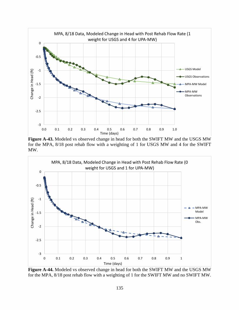
135
Figure A-43. Modeled vs observed change in head for both the SWIFT MW and the USGS MW
for the MPA, 8/18 post rehab flow with a weighting of 1 for USGS MW and 4 for the SWIFT
MW.
Figure A-44. Modeled vs observed change in head for both the SWIFT MW and the USGS MW
for the MPA, 8/18 post rehab flow with a weighting of 1 for the SWIFT MW and no SWIFT MW.
-3
-2.5
-2
-1.5
-1
-0.5
0
0.0 0.1 0.2 0.3 0.4 0.5 0.6 0.7 0.8 0.9 1.0
Ch
ange
in H
ead
(ft
)
Time (days)
MPA, 8/18 Data, Modeled Change in Head with Post Rehab Flow Rate (1 weight for USGS and 4 for UPA-MW)
USGS Model
USGS Observations
MPA-MW Model
MPA-MWObservations
-3
-2.5
-2
-1.5
-1
-0.5
0
0 0.1 0.2 0.3 0.4 0.5 0.6 0.7 0.8 0.9 1
Ch
ange
in H
ead
(ft
)
Time (days)
MPA, 8/18 Data, Modeled Change in Head with Post Rehab Flow Rate (0 weight for USGS and 1 for UPA-MW)
MPA-MWModel
MPA-MWObs.

136
Figure A-45. Modeled vs observed change in head for both the SWIFT MW and the USGS MW
for the MPA, 4/19 pre-rehab flow using the hydrogeological parameters from the MPA, 8/18 pre-
rehab flow model with a weighting of 1 for USGS MW and 4 for the SWIFT MW.
Figure A-46. Modeled vs observed change in head for both the SWIFT MW and the USGS MW
for the MPA, 4/19 pre-rehab flow with equal weighting for each observation point.
-2
-1.5
-1
-0.5
0
0 0.1 0.2 0.3
Ch
ange
in H
ead
(ft
)
Time (days)
MPA 4/19 Ob. Data Modeled with Pre-rehab Flow Rate and 8/18 Pre-rehab Hydraulic Parameters
USGS Model
USGS Observations
MPA-MW Model
MPA-MWObservations
-2
-1.5
-1
-0.5
0
0 0.1 0.2 0.3
Ch
ange
in H
ead
(ft
)
Time (days)
MPA, 4/19 Data, Modeled Change in Head with Pre-rehab Flow Rate (Equally Weighted)
USGS Model
USGS Observations
MPA-MW Model
MPA-MWObservations
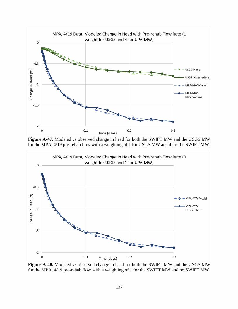
137
Figure A-47. Modeled vs observed change in head for both the SWIFT MW and the USGS MW
for the MPA, 4/19 pre-rehab flow with a weighting of 1 for USGS MW and 4 for the SWIFT MW.
Figure A-48. Modeled vs observed change in head for both the SWIFT MW and the USGS MW
for the MPA, 4/19 pre-rehab flow with a weighting of 1 for the SWIFT MW and no SWIFT MW.
-2
-1.5
-1
-0.5
0
0 0.1 0.2 0.3
Ch
ange
in H
ead
(ft
)
Time (days)
MPA, 4/19 Data, Modeled Change in Head with Pre-rehab Flow Rate (1 weight for USGS and 4 for UPA-MW)
USGS Model
USGS Observations
MPA-MW Model
MPA-MWObservations
-2
-1.5
-1
-0.5
0
0 0.1 0.2 0.3
Ch
ange
in H
ead
(ft
)
Time (days)
MPA, 4/19 Data, Modeled Change in Head with Pre-rehab Flow Rate (0 weight for USGS and 1 for UPA-MW)
MPA-MW Model
MPA-MWObservations
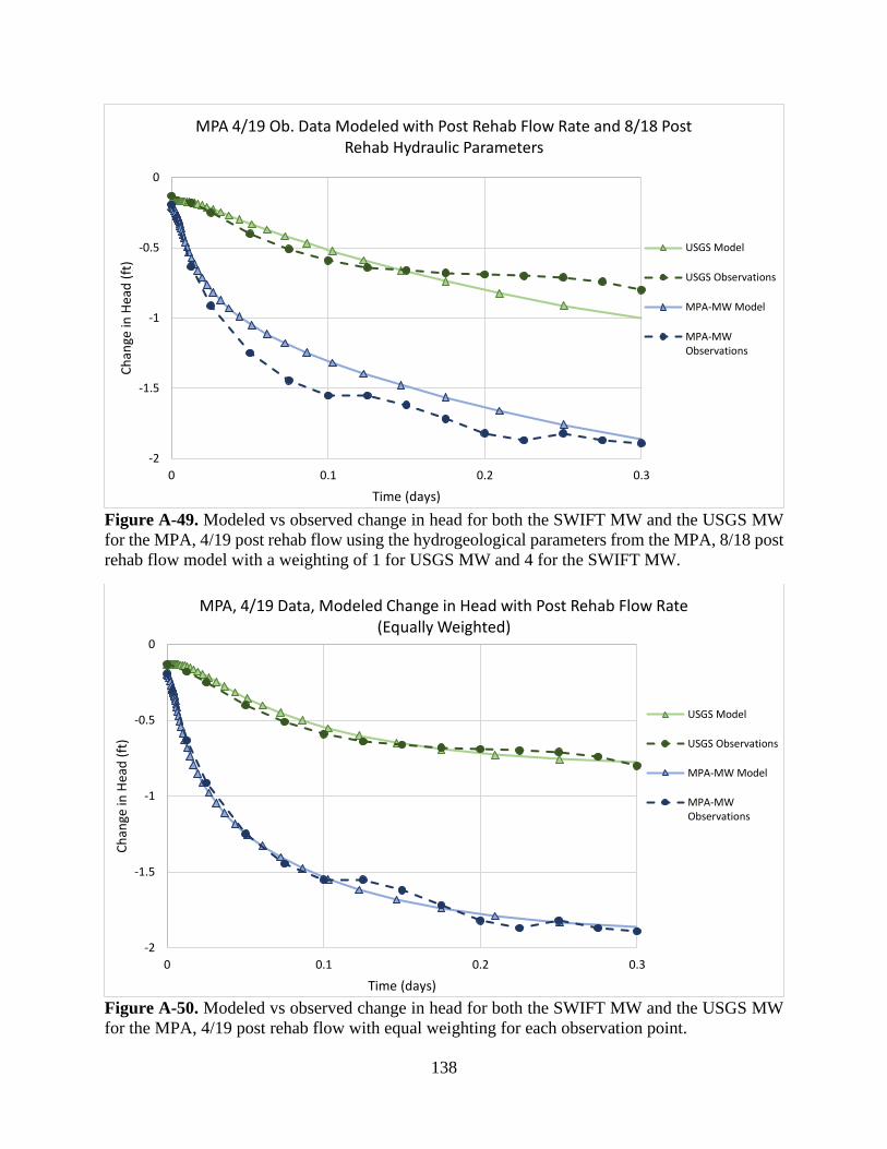
138
Figure A-49. Modeled vs observed change in head for both the SWIFT MW and the USGS MW
for the MPA, 4/19 post rehab flow using the hydrogeological parameters from the MPA, 8/18 post
rehab flow model with a weighting of 1 for USGS MW and 4 for the SWIFT MW.
Figure A-50. Modeled vs observed change in head for both the SWIFT MW and the USGS MW
for the MPA, 4/19 post rehab flow with equal weighting for each observation point.
-2
-1.5
-1
-0.5
0
0 0.1 0.2 0.3
Ch
ange
in H
ead
(ft
)
Time (days)
MPA 4/19 Ob. Data Modeled with Post Rehab Flow Rate and 8/18 Post Rehab Hydraulic Parameters
USGS Model
USGS Observations
MPA-MW Model
MPA-MWObservations
-2
-1.5
-1
-0.5
0
0 0.1 0.2 0.3
Ch
ange
in H
ead
(ft
)
Time (days)
MPA, 4/19 Data, Modeled Change in Head with Post Rehab Flow Rate (Equally Weighted)
USGS Model
USGS Observations
MPA-MW Model
MPA-MWObservations
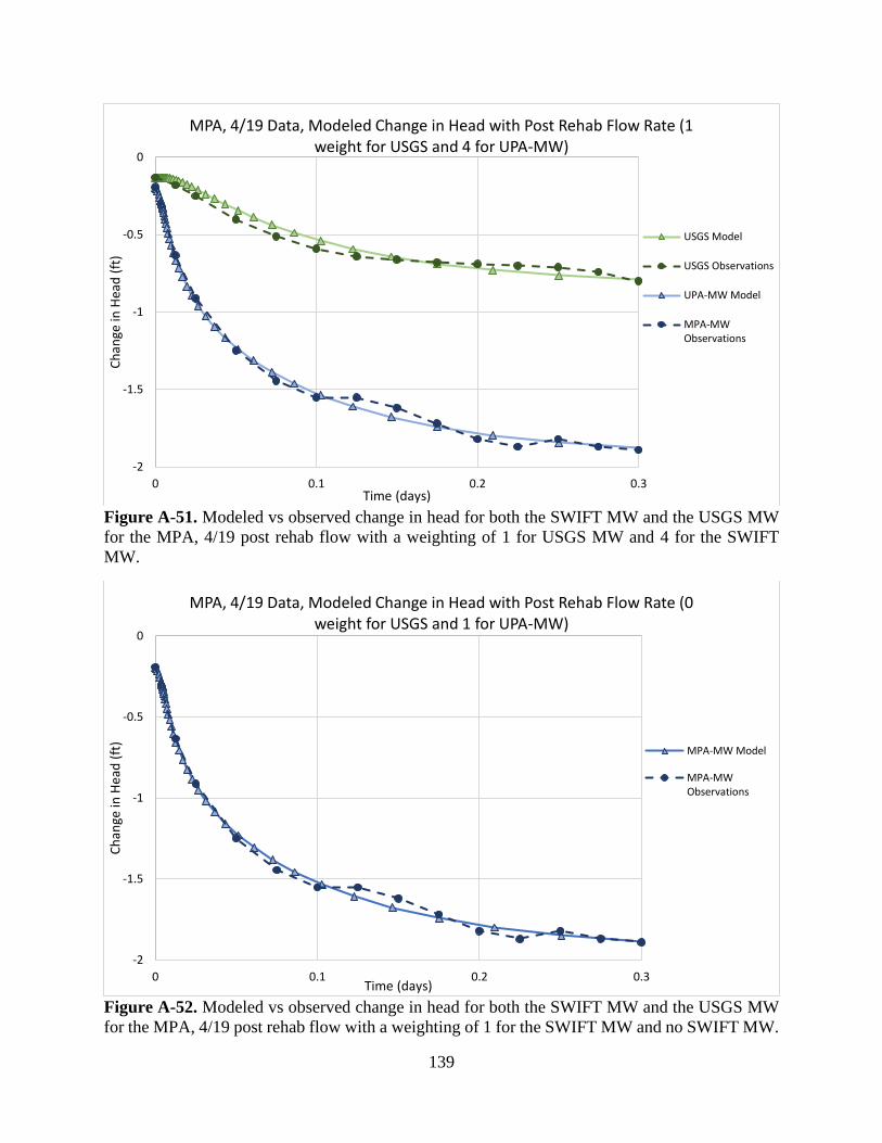
139
Figure A-51. Modeled vs observed change in head for both the SWIFT MW and the USGS MW
for the MPA, 4/19 post rehab flow with a weighting of 1 for USGS MW and 4 for the SWIFT
MW.
Figure A-52. Modeled vs observed change in head for both the SWIFT MW and the USGS MW
for the MPA, 4/19 post rehab flow with a weighting of 1 for the SWIFT MW and no SWIFT MW.
-2
-1.5
-1
-0.5
0
0 0.1 0.2 0.3
Ch
ange
in H
ead
(ft
)
Time (days)
MPA, 4/19 Data, Modeled Change in Head with Post Rehab Flow Rate (1 weight for USGS and 4 for UPA-MW)
USGS Model
USGS Observations
UPA-MW Model
MPA-MWObservations
-2
-1.5
-1
-0.5
0
0 0.1 0.2 0.3
Ch
ange
in H
ead
(ft
)
Time (days)
MPA, 4/19 Data, Modeled Change in Head with Post Rehab Flow Rate (0 weight for USGS and 1 for UPA-MW)
MPA-MW Model
MPA-MWObservations
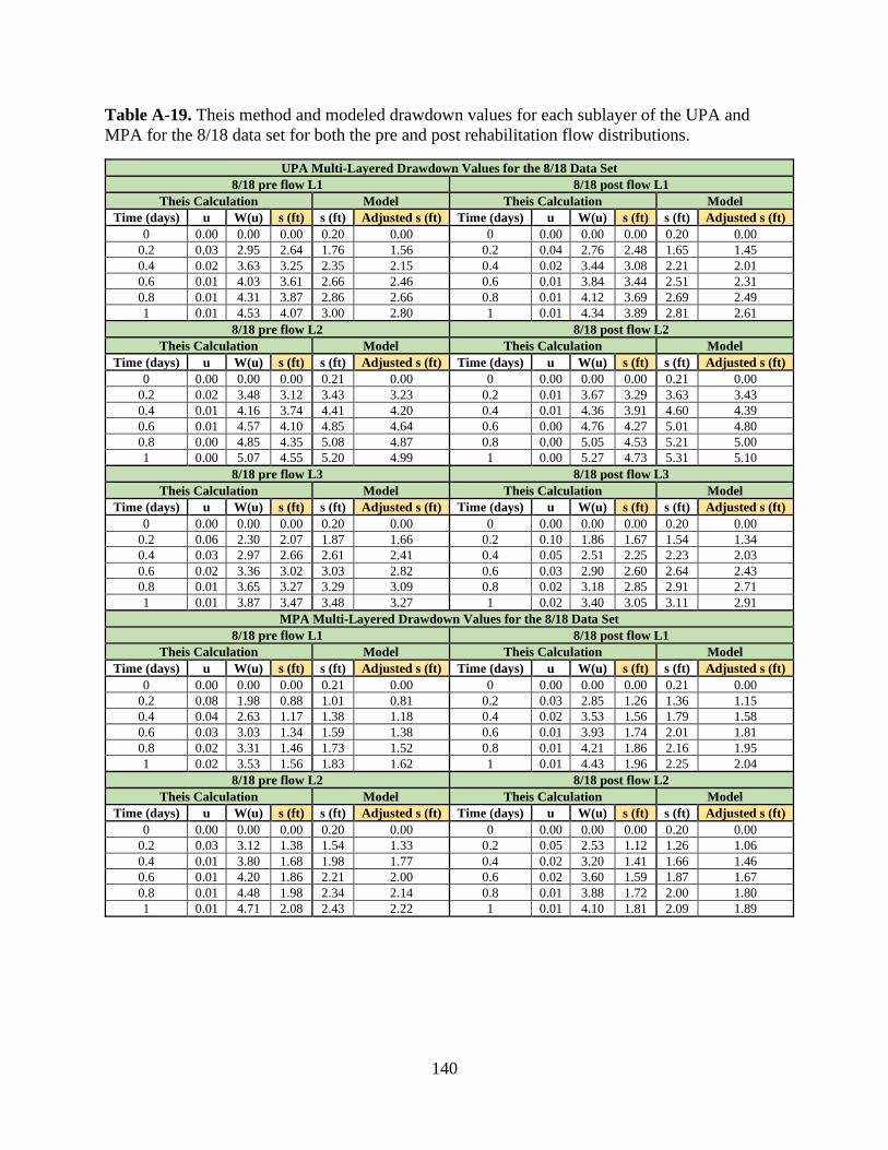
140
Table A-19. Theis method and modeled drawdown values for each sublayer of the UPA and
MPA for the 8/18 data set for both the pre and post rehabilitation flow distributions.
UPA Multi-Layered Drawdown Values for the 8/18 Data Set
8/18 pre flow L1 8/18 post flow L1
Theis Calculation Model Theis Calculation Model
Time (days) u W(u) s (ft) s (ft) Adjusted s (ft) Time (days) u W(u) s (ft) s (ft) Adjusted s (ft)
0 0.00 0.00 0.00 0.20 0.00 0 0.00 0.00 0.00 0.20 0.00
0.2 0.03 2.95 2.64 1.76 1.56 0.2 0.04 2.76 2.48 1.65 1.45
0.4 0.02 3.63 3.25 2.35 2.15 0.4 0.02 3.44 3.08 2.21 2.01
0.6 0.01 4.03 3.61 2.66 2.46 0.6 0.01 3.84 3.44 2.51 2.31
0.8 0.01 4.31 3.87 2.86 2.66 0.8 0.01 4.12 3.69 2.69 2.49
1 0.01 4.53 4.07 3.00 2.80 1 0.01 4.34 3.89 2.81 2.61
8/18 pre flow L2 8/18 post flow L2
Theis Calculation Model Theis Calculation Model
Time (days) u W(u) s (ft) s (ft) Adjusted s (ft) Time (days) u W(u) s (ft) s (ft) Adjusted s (ft)
0 0.00 0.00 0.00 0.21 0.00 0 0.00 0.00 0.00 0.21 0.00
0.2 0.02 3.48 3.12 3.43 3.23 0.2 0.01 3.67 3.29 3.63 3.43
0.4 0.01 4.16 3.74 4.41 4.20 0.4 0.01 4.36 3.91 4.60 4.39
0.6 0.01 4.57 4.10 4.85 4.64 0.6 0.00 4.76 4.27 5.01 4.80
0.8 0.00 4.85 4.35 5.08 4.87 0.8 0.00 5.05 4.53 5.21 5.00
1 0.00 5.07 4.55 5.20 4.99 1 0.00 5.27 4.73 5.31 5.10
8/18 pre flow L3 8/18 post flow L3
Theis Calculation Model Theis Calculation Model
Time (days) u W(u) s (ft) s (ft) Adjusted s (ft) Time (days) u W(u) s (ft) s (ft) Adjusted s (ft)
0 0.00 0.00 0.00 0.20 0.00 0 0.00 0.00 0.00 0.20 0.00
0.2 0.06 2.30 2.07 1.87 1.66 0.2 0.10 1.86 1.67 1.54 1.34
0.4 0.03 2.97 2.66 2.61 2.41 0.4 0.05 2.51 2.25 2.23 2.03
0.6 0.02 3.36 3.02 3.03 2.82 0.6 0.03 2.90 2.60 2.64 2.43
0.8 0.01 3.65 3.27 3.29 3.09 0.8 0.02 3.18 2.85 2.91 2.71
1 0.01 3.87 3.47 3.48 3.27 1 0.02 3.40 3.05 3.11 2.91
MPA Multi-Layered Drawdown Values for the 8/18 Data Set
8/18 pre flow L1 8/18 post flow L1
Theis Calculation Model Theis Calculation Model
Time (days) u W(u) s (ft) s (ft) Adjusted s (ft) Time (days) u W(u) s (ft) s (ft) Adjusted s (ft)
0 0.00 0.00 0.00 0.21 0.00 0 0.00 0.00 0.00 0.21 0.00
0.2 0.08 1.98 0.88 1.01 0.81 0.2 0.03 2.85 1.26 1.36 1.15
0.4 0.04 2.63 1.17 1.38 1.18 0.4 0.02 3.53 1.56 1.79 1.58
0.6 0.03 3.03 1.34 1.59 1.38 0.6 0.01 3.93 1.74 2.01 1.81
0.8 0.02 3.31 1.46 1.73 1.52 0.8 0.01 4.21 1.86 2.16 1.95
1 0.02 3.53 1.56 1.83 1.62 1 0.01 4.43 1.96 2.25 2.04
8/18 pre flow L2 8/18 post flow L2
Theis Calculation Model Theis Calculation Model
Time (days) u W(u) s (ft) s (ft) Adjusted s (ft) Time (days) u W(u) s (ft) s (ft) Adjusted s (ft)
0 0.00 0.00 0.00 0.20 0.00 0 0.00 0.00 0.00 0.20 0.00
0.2 0.03 3.12 1.38 1.54 1.33 0.2 0.05 2.53 1.12 1.26 1.06
0.4 0.01 3.80 1.68 1.98 1.77 0.4 0.02 3.20 1.41 1.66 1.46
0.6 0.01 4.20 1.86 2.21 2.00 0.6 0.02 3.60 1.59 1.87 1.67
0.8 0.01 4.48 1.98 2.34 2.14 0.8 0.01 3.88 1.72 2.00 1.80
1 0.01 4.71 2.08 2.43 2.22 1 0.01 4.10 1.81 2.09 1.89

141
Table A-20. Theis method and modeled drawdown values for each sublayer of the UPA and
MPA for the 4/19 data set for both the pre and post rehabilitation flow distributions.
UPA Multi-Layered Drawdown Values for the 4/19 Data Set
4/19 pre flow L1 4/19 post flow L1
Theis Calculation Model Theis Calculation Model
Time (days) u W(u) s (ft) s (ft) Adjusted s (ft) Time (days) u W(u) s (ft) s (ft) Adjusted s (ft)
0 0.00 0.00 0.00 0.20 0.00 0 0.00 0.00 0.00 0.20 0.00
0.2 0.02 3.29 2.14 1.45 1.25 0.2 0.03 3.11 2.01 1.37 1.18
0.4 0.01 3.97 2.58 1.83 1.63 0.4 0.01 3.79 2.45 1.75 1.56
0.6 0.01 4.37 2.84 1.99 1.79 0.6 0.01 4.19 2.71 1.92 1.72
0.8 0.01 4.66 3.03 2.06 1.86 0.8 0.01 4.48 2.90 2.00 1.80
1 0.00 4.88 3.17 2.10 1.90 1 0.01 4.70 3.04 2.04 1.84
4/19 pre flow L2 4/19 post flow L2
Theis Calculation Model Theis Calculation Model
Time (days) u W(u) s (ft) s (ft) Adjusted s (ft) Time (days) u W(u) s (ft) s (ft) Adjusted s (ft)
0 0.00 0.00 0.00 0.21 0.00 0 0.00 0.00 0.00 0.21 0.00
0.2 0.01 3.82 2.48 2.68 2.48 0.2 0.01 4.03 2.61 2.81 2.60
0.4 0.01 4.51 2.93 3.23 3.02 0.4 0.01 4.71 3.05 3.33 3.12
0.6 0.00 4.91 3.19 3.40 3.19 0.6 0.00 5.12 3.31 3.48 3.27
0.8 0.00 5.20 3.38 3.46 3.25 0.8 0.00 5.40 3.50 3.53 3.32
1 0.00 5.42 3.52 3.48 3.27 1 0.00 5.63 3.64 3.55 3.34
4/19 pre flow L3 4/19 post flow L3
Theis Calculation Model Theis Calculation Model
Time (days) u W(u) s (ft) s (ft) Adjusted s (ft) Time (days) u W(u) s (ft) s (ft) Adjusted s (ft)
0 0.00 0.00 0.00 0.20 0.00 0 0.00 0.00 0.00 0.20 0.00
0.2 0.04 2.64 1.71 1.59 1.39 0.2 0.07 2.19 1.42 1.34 1.13
0.4 0.02 3.31 2.15 2.13 1.93 0.4 0.03 2.86 1.85 1.86 1.66
0.6 0.01 3.71 2.41 2.39 2.19 0.6 0.02 3.25 2.10 2.15 1.94
0.8 0.01 3.99 2.59 2.54 2.33 0.8 0.02 3.53 2.29 2.33 2.12
1 0.01 4.21 2.74 2.62 2.42 1 0.01 3.75 2.43 2.45 2.24
MPA Multi-Layered Drawdown Values for the 4/19 Data Set
4/19 pre flow L1 4/19 post flow L1
Theis Calculation Model Theis Calculation Model
Time (days) u W(u) s (ft) s (ft) Adjusted s (ft) Time (days) u W(u) s (ft) s (ft) Adjusted s (ft)
0 0.00 0.00 0.00 0.21 0.00 0 0.00 0.00 0.00 0.21 0.00
0.2 0.07 2.19 1.07 1.20 1.00 0.2 0.03 3.07 1.50 1.56 1.35
0.4 0.03 2.85 1.40 1.61 1.41 0.4 0.01 3.75 1.84 1.94 1.73
0.6 0.02 3.25 1.59 1.82 1.62 0.6 0.01 4.15 2.03 2.08 1.88
0.8 0.02 3.53 1.73 1.94 1.74 0.8 0.01 4.44 2.17 2.14 1.94
1 0.01 3.75 1.84 2.02 1.81 1 0.01 4.66 2.28 2.17 1.96
4/19 pre flow L2 4/19 post flow L2
Theis Calculation Model Theis Calculation Model
Time (days) u W(u) s (ft) s (ft) Adjusted s (ft) Time (days) u W(u) s (ft) s (ft) Adjusted s (ft)
0 0.00 0.00 0.00 0.20 0.00 0 0.00 0.00 0.00 0.20 0.00
0.2 0.02 3.34 1.63 1.68 1.48 0.2 0.04 2.75 1.34 1.44 1.24
0.4 0.01 4.02 1.97 2.03 1.83 0.4 0.02 3.42 1.67 1.83 1.64
0.6 0.01 4.42 2.17 2.15 1.95 0.6 0.01 3.82 1.87 2.00 1.80
0.8 0.01 4.71 2.31 2.19 1.99 0.8 0.01 4.10 2.01 2.08 1.88
1 0.00 4.93 2.41 2.21 2.01 1 0.01 4.33 2.12 2.11 1.91
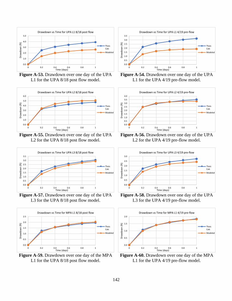
142
Figure A-53. Drawdown over one day of the UPA
L1 for the UPA 8/18 post flow model.
Figure A-54. Drawdown over one day of the UPA
L1 for the UPA 4/19 pre-flow model.
Figure A-55. Drawdown over one day of the UPA
L2 for the UPA 8/18 post flow model.
Figure A-56. Drawdown over one day of the UPA
L2 for the UPA 4/19 pre-flow model.
Figure A-57. Drawdown over one day of the UPA
L3 for the UPA 8/18 post flow model.
Figure A-58. Drawdown over one day of the UPA
L3 for the UPA 4/19 pre-flow model.
Figure A-59. Drawdown over one day of the MPA
L1 for the UPA 8/18 post flow model.
Figure A-60. Drawdown over one day of the MPA
L1 for the UPA 4/19 pre-flow model.
0.0
1.0
2.0
3.0
4.0
5.0
0 0.2 0.4 0.6 0.8 1
Dra
wd
ow
n (
ft)
Time (days)
Drawdown vs Time for UPA L1 8/18 post flow
TheisCalc
Modeled
0.0
0.5
1.0
1.5
2.0
2.5
3.0
3.5
0 0.2 0.4 0.6 0.8 1
Dra
wd
ow
n (
ft)
Time (days)
Drawdown vs Time for UPA L1 4/19 pre-flow
TheisCalc
Modeled
0.0
1.0
2.0
3.0
4.0
5.0
6.0
0 0.2 0.4 0.6 0.8 1
Dra
wd
ow
n (
ft)
Time (days)
Drawdown vs Time for UPA L2 8/18 post flow
TheisCalc
Modeled
0.0
0.5
1.0
1.5
2.0
2.5
3.0
3.5
4.0
0 0.2 0.4 0.6 0.8 1
Dra
wd
ow
n (
ft)
Time (days)
Drawdown vs Time for UPA L2 4/19 pre-flow
TheisCalc
Modeled
0.0
0.5
1.0
1.5
2.0
2.5
3.0
3.5
0 0.2 0.4 0.6 0.8 1
Dra
wd
ow
n (
ft)
Time (days)
Drawdown vs Time for UPA L3 8/18 post flow
TheisCalc
Modeled
0.0
0.5
1.0
1.5
2.0
2.5
3.0
0 0.2 0.4 0.6 0.8 1
Dra
wd
ow
n (
ft)
Time (days)
Drawdown vs Time for UPA L3 4/19 pre-flow
TheisCalc
Modeled
0.0
0.5
1.0
1.5
2.0
2.5
0 0.2 0.4 0.6 0.8 1
Dra
wd
ow
n (
ft)
Time (days)
Drawdown vs Time for MPA L1 8/18 post flow
TheisCalc
Modeled
0.0
0.5
1.0
1.5
2.0
0 0.2 0.4 0.6 0.8 1
Dra
wd
ow
n (
ft)
Time (days)
Drawdown vs Time for MPA L1 4/19 pre-flow
TheisCalc
Modeled
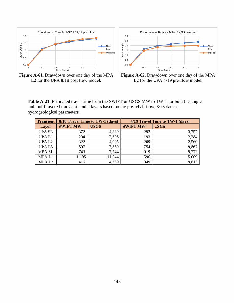
143
Figure A-61. Drawdown over one day of the MPA
L2 for the UPA 8/18 post flow model.
Figure A-62. Drawdown over one day of the MPA
L2 for the UPA 4/19 pre-flow model.
Table A-21. Estimated travel time from the SWIFT or USGS MW to TW-1 for both the single
and multi-layered transient model layers based on the pre-rehab flow, 8/18 data set
hydrogeological parameters.
Transient 8/18 Travel Time to TW-1 (days) 4/19 Travel Time to TW-1 (days)
Layer SWIFT MW USGS SWIFT MW USGS
UPA SL 372 4,839 292 3,757
UPA L1 204 2,395 193 2,284
UPA L2 322 4,005 209 2,560
UPA L3 597 7,859 754 9,867
MPA SL 743 7,544 919 9,273
MPA L1 1,195 11,244 596 5,669
MPA L2 416 4,339 949 9,813
0.0
0.5
1.0
1.5
2.0
0 0.2 0.4 0.6 0.8 1
Dra
wd
ow
n (
ft)
Time (days)
Drawdown vs Time for MPA L2 8/18 post flow
TheisCalc
Modeled
0.0
0.5
1.0
1.5
2.0
2.5
3.0
0 0.2 0.4 0.6 0.8 1
Dra
wd
ow
n (
ft)
Time (days)
Drawdown vs Time for MPA L2 4/19 pre-flow
TheisCalc
Modeled