ficrhod I arha ao - VTechWorks
182
THE FINITE ELEMENT ANALYSIS OF LAMINATED COMPOSITES by Fu Tien Lin Thesis submitted to the Graduate Faculty of the Virginia Polytechnic Institute and State University in partial fulfillment of the requirements for the degree of | DOCTOR OF PHILOSOPHY in Engineering Mechanics APPROVED: Beel Crekonek Daniel Frederick, Chairman ficrhod I arha ao Richard M. Barker Robert A. ten [PROe &. cay i! | 7 tah we / "| December, 1971 Blacksburg, Virginia
-
Upload
khangminh22 -
Category
Documents
-
view
0 -
download
0
Transcript of ficrhod I arha ao - VTechWorks

THE FINITE ELEMENT ANALYSIS OF LAMINATED COMPOSITES
by
Fu Tien Lin
Thesis submitted to the Graduate Faculty of the
Virginia Polytechnic Institute and State University
in partial fulfillment of the requirements for the degree of |
DOCTOR OF PHILOSOPHY
in
Engineering Mechanics
APPROVED: Beel Cr ekonek Daniel Frederick, Chairman
ficrhod I arha ao Richard M. Barker Robert A. ten
[PROe &. cay i! | 7 tah we / "|
December, 1971
Blacksburg, Virginia

LD 5055 V856 1g7! Ls4 Q, a
S
ACKNOWLEDGEMENTS
This investigation was supported by the Department of Defense,
Project THEMIS, Contract Number DAA FO7-69-C-O449 with Watervliet Arsenal,
Watervliet, New York.
The author expresses his sincere appreciation to Dr. Daniel
Frederick, Director of Project THEMTS and Chairman of his committee for
providing guidance and enccuragement throughout the investigation.
Special thanks must go to Dr. Richard M. Barker for his help and
advice in this investigation. Thanks are also extended to members of
his graduate committee for the assistance they have provided during his
study at Virginia Polytechnic Institute and State University.
Also, the patience and support of the author's wife, Chii Mei,
is gratefully acknowledged.
ii

TABLE OF CONTENTS
*
Chapter
LIST OF FIGURES . 2. 1. 6 6 we ew we we ee
LIST OF TABLES . 2. 2. 2 «© «© © © © © © we ow oe
LIST OF SYMBOLS . . 2. 2. 2 2 0 2 0 ew ew ew ew .
I. INTRODUCTION . 6. 6 6 6 ww we ew te we tw
II. REVIEW OF LITERATURE . . 2. 1 6 «© 2 oe we ow .
IfI. ANALYTICAL METHOD... 2... 1. 2 es ew we 2
A. Development of the Governing Equations for a Lamina
Assumptions and Definitions ........ . Hellinger-Reissner Variational Principle. . Equations of Motion ..... oe oe
Stress Resultant-Displacement Relations hips .
Basic Equations for the Bending of Rectangular Plates Governing Equations for the Extension of Plates .
B. Cylindrical Bending of a Two-Ply Laminate oe
Examples and Discussion . ... 2.4 1 6 6» . Fourier Series Representation for a Uniform Load
IV. PINITE ELEMENTS IN TWO DIMENSIONS ..... ar
A. 16-DOF Element Formulation .....e...
Displacement Functions .. oe ew
Derivation of Element Stiffness Matrix. . .
Consistent Element Joint Loads. ......
Trace of the Element Stiffness Matrix...
Assembly and Analysis .....
24U-DOF Element Formulation. ...... «ee
Shape Functions . . 1. 2. 1 6 © ew ew ee Coordinate Trans formation oe 8 ee ew ee
Element Stiffness Matrix. woe
Trace of the Element Stiffness Matrix...
Consistent EDlement Joint Loads. . ....-.
Stress Analy ais 2 e * * . . ° e * ° ° . . e
iii
Page
LO
LO
10
13
17
18
18
20
22
36
38
39
Wi
42
43
uy.
uy 47 4g 49 50
YY a

iv
Chapter
V.
VI.
C. Applications and Discussion...
Aluminum-Steel Laminate in Cylindrical Bending. . . 2-Ply Laminate ......6. +66. 3-Ply Laminate . . « e . ° ° ° * + e
FINITE ELEMENTS IN THREE DIMENSIONS .
Shape Function for 72-DOF Element .
Coordinate Transformation .
The Elasticity Matrix ........
Element Stiffness Matrix ......
Trace of the Stiffness Matrix...
Consistent Element Joint Loads. ...
Application and Discussion .....
CONCLUSIONS . 2. 2 6 0 we we ew ew et
BIBLIOGRAPHY . 2. 2. 2 2 2 6 ee we ew ww
APPENDICES . 2. 2. 6. © 6 6 1 oe ew ew ew
A. The elements of selected matrices
B, The elements of selected matrices
C. 16-DOF Program Listing. .....
D. 24-DOF Program Listing. .....
E. 72-DOF Program Listing. .....
VITA . 6 6 ww ew ww ew ww ee
e ° ° cd
used in
used in
Chapter
Chapter
Page
52
52 56
58
61
61
63
65
67
69
69
73
78
80
83
83
85

Figure
1. Laminate, Lamina and Element of the Lamina .......
2. Aluminum-Steel Laminate in Cylindrical Bending .....
3. Displacement and Stress Distributions for Aluminum-Steel Laminate, hy = 1", hy = .5",s = 10 ....64608446-4
4, Fourier Series Expansion for Uniform Load q=i1.....
5. 16-DOF Element, Distributed Force and Trace. ......
6. 24-DOF Element, 4# x 4 Gauss Rule and Trace .......
7. Consistent Element Joint Loads for Cubic Curve Line. .
8. Stress Distributions for Aluminum-Steel Laminate in Cylin- drical Bending by Sinusoidal Load, s=10......
9, Stress Distributions for Aluminum-Steel Laminate in Cylin- drical Bending by Uniform Load, s = 10 ce ee ew
10. Stress Distributions for 2-Ply Laminate in Cylindrical Bending by Sinusoidal Load, s=4 ...... 2. 2 ee
ll. Displacement and Stress Distributions for 3-Ply Leminate in Cylindrical Bending by Sinusoidal Load, s =4....
12. 72-DOF Element, Parent Elements and Trace of Right Prism
13. Consistent Element Joint Loads for Distributed Surface Load.
14. Symmetric 3-Ply Square Laminate and Idealization....
15. Stress and Displacement Distributions in Symmetric 3-Ply
LIST OF FIGURES
Square Laminate . 1... 6 6 ee ee ew we ew we
7
Page
Li
» 23
*.
30
31
37
45
51
53
54
57
59
62
- 71
- 74
- 77
Table
Il.
Itt.
IV.
LIST OF TABLES
Page
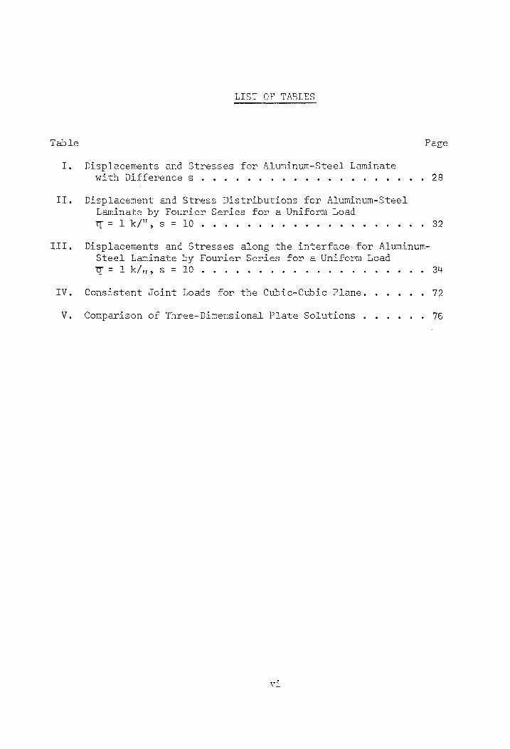
Displacements and Stresses for Aluminum-Steel Laminate with Difference S . 1 1 1 6 ew ew ew ew ww ew ww ww ww 28
Displacement and Stress Distributions for Aluminum-Steel Laminate by Fourier Series for a Uniform Load dT=1k/", s = 10 ° ° * . e e * . ° ° e e e e o . . . e e 32
Displacements and Stresses along the interface for Aluminum- Steel Laminate by Fourier Series for a Uniform Load @Q@=1k/n,s = 10 ° e s * * . . ° e e e e * ° ° . e ° eo ° 34
Consistent Joint Loads for the Cubic-Cubic Plane. ..... 72
Comparison of Three-Dimensional Plate Solutions ...... 76
Vi

LIST OF SYMBOLS
Lamina principal directions
Element side lengths in x, y, z directions
Direction cosines for angle between lamina and
global axes
Flexural rigidity
Modulus of elasticity for isotropic material
Shear modulus for isotropic material
Plate thickness
Weighing coefficients for Gaussian points
Kinetic energy
Length of a side of an element
cos 8, sin 6 respectively where § is the angle between lamina and global axes
Bending stress resultants
Total number of layers in a laminate
In-plane stress resultants
Intensity of distributed load
pistributed load
Maximum intensity of sinusoidal distributed load
Boundary surface on which stress prescribed
Boundary surface on which displacement prescribed
T B T + B. ot T xT T tT 5
B e
+ o_, respectively XZ XZ, YZ Vz Z Z
Shear stress resultants
vii

u, V,
Us, Vs, W
Xs Vo Zz
W
aq.
a, Bs, ¥
E,n, sf
O19 Oy» o
T 3 XY XZ
f°? € >
Yay? _
rt ce XZ? yz? B B
T 4 iT XZ yz
O.. 1]
E..
1)
Vv
U..
LJ
0
fA]
[Bq
[c]
[DJ
= |
vill
Displacement functions at the micplane in x, y, z direction
Displacements of a point in x, y, z directions
Global cartesian coordinates
Mixed strain energy density function
Constants in displacement functions
Linear term of u, v, w expansion
Local curvilinear coordinates
Normal stress components with respect to global system
Shear stress components with respect to global system
Normal strain components with respect to global system
Shear strain components with respect to global system
Stresses at the top face of lamina
Stresses at the bottom face of lamina
Stresses in constitutive relations for an anisotropic material
Strains in constitutive relations for an anisotropic material
Poisson's ratio for isotropic material
Poisson's ratio relating normal strain in j-direction due to uniaxial normal stress in i-direction
Mass density per unit volume
Matrix relating nodal displacements to constant
Matrix relating strains to nodal displacements
Matrix representing differentiation of {N} with respect
to Es ns Z
Elasticity matrix

—{£}
{PF}
[J]
[k]
[Kk]
[M]
{Nn}
{Pp}
fu,}
fu}
[XyzJ
{a}
fe}
{a}
ix
Element nodal force vector
Global force vector
Jacobian Matrix
Determinate of [J]
Element stiffness matrix
Global stiffness matrix
Matrix relating displacement matrix {u} to constant matrix {a}
Shape functions
Consistent element joint loads vector
Element displacement vector
Global displacement vector
Matrix representing element node global coordinates
vector of stress
Vector of strain
Matrix representing constants in displacement functions

I. INTRODUCTION
A composite material consists of high strength, continuous or
discontinuous filaments embedded in matrix material. Filament materials
which have been used widely are glass, steel, boron and graphite; and
matrix materials in use are aluminum, epoxies, epoxy phenolics. When a
composite is subjected to external loads the matrix transfers stresses
to the embedded high strength fibers. With such a configuration of
filaments and matrix, a high strength-to-weight ratio is achieved. Com-
mon applications of composites are for aircraft, space vehicle and deep
sea structures.
There are various kinds of constituent materials and many options
in the fiber arrangements of a lamina, and in lamina orientations of a
composite. Of the different combi ations for a composite, one may design
a composite such that the laminas are oricnted in an optimum manner with
respect to some prescribed design criteria.
An individual lamina, or basic ply, of a multilayered composite
is considered to be a homogeneous and orthotropic material. But the
layered laminate, which is formed by bonding arbitrary oriented laminas
in the form of laminated composite plates and shells, in a complex, non-
homogeneous, anisotropic structure.
Classical laminated plate theories (CPT) have been used to analyze
composite structures and some boundary value problems have been formulated
and solved. Owing to certain assumptions of CPT, such as the classical
small deformation assumption, the results for deformation and stress

distributions have not been in good agreement with the exact elasticity
solutions. Although some recent exact solutions are available, they are
restricted to certain special types of boundary value problems.
It is the purpose of this dissertation to present a truly three
dimensional finite element analysis for laminated composites which re-
moves the undesirable restrictions existing in the CPT and some refined
theories. The basic restriction, which is one straight line normal ro-
tation through the plate thickness, is removed by taking a linear varia-
tion of displacements through the element thickness and using one or
more elements for each layer of the laminate. Thus a complete three-
dimensional analysis of the composite is developed which includes the
thickness-stretching deformation as well as extension deformation, and
transverse shear strains. Most of the problems solved by the CPT, re-
fined theories and exact elasticity theory have been for rectangular
plates with simply-supported edges. In this study generality is achieved
by using a curved isoparametric element with cubic displacements expan-
Sion in plane which enables the element to fit boundaries of arbitrary
shape.
Prior to presenting the two- and three-dimensional finite element
analyses of laminated composites, an analytical method for composite with
isotropic lamina is presented. A linear expansion for displacements is
assumed in each lamina. By applying the Hellinger-Reissner variational
principle, governing equations for bending and extensicn are derived.
Because of the complexity of the governing equations and difficulty of
achieving exact solutions, the equations for the three-dimensional prob-
lem are specialized to the two-dimensional case of cylindrical bending.

Solutions are obtained in this case for sinusoidal and uniform loadings.
A Fourier series solution is obtained for the latter.
Two elements are developed for the finite element analysis of
two-dimensional laminated composites. Because the plate bending is
usually associated with cubic displacement functions, and the individual
layers of laminated plates are relatively thin compared with the other
dimensions of plate, a 16 degree of freedom (DOF) element is presented
first. A cubic expansion of displacements in the plane direction and a
linear variation of displacements through the thickness of the element
are used. In order to evaluate the performance of the 16-DOF element, a
24-DOF element is developed for which a cubic expansion of displacements
in the thickness direction is employed. In the 16-DOF element, rectangu-
lar cartesian coordinates are used and the element stiffness matrix is
formulated directly and explicitly for a rectangular element. In the
24H-DOF element, a local curvilinear coordinates are used to describe the
nodal displacements of the element and its geometry, and a numerical in-
tegration procedure is applied to formulate the element stiffness matrix.
Results of the finite element analyses are compared with the solutions by
an analytical method and, wherever possible, with an exact elasticity
solution.
A curved, isoparametric, 72-DOF element is developed for the
three-dimensional finite element analysis of the laminated composites.
The displacement expansion is the three-dimensional analog of the 16-DOF
element, that is, a cubic expansion of the displacement in the element
plane and a linear variation of displacement through the thickness of the

element are made. A numerical integration procedure is employed to formu-
late the element stiffness matrix. Fesults are compared with the exact
elasticity solution.
It is believed that the refined, curved, isoparametric element
to be presented herein offers an improvement over the simple, linear
triangular and quadrilateral elements and that the finite element method
facilitates the investigation of the arbitrary shaped layered composites.
Furthermore the applicability of the solutions for the laminated compo-
sites can be expanded to more general fields.

II. REVIEW OF LITERATURE
The first report on composite plates laminated with thin ortho-
tropic layers or plies was published by Smith [g]* in 1953. Reissner
and Stavsky [10] were first to recognize the coupling phenomenon between
in-plane stretching and transverse bending for nonsymmetrical laminated
plates. This phenomenon does not occur in the theory of homogeneous
plates and had been overlooked by Smith. The coupling effect was pre-
sented by considering two orthotropic layers of equal thickness laminated
in such a way that the axes of elastic symmetry are located at an angle
of +8 with the plate axes in one layer and an angle of -@ in the other
layer. Results obtained by considering coupling were quite different
from those obtained without coupling.
In 1962, a general small-deflecticn theory for the elastostatic
extension and flexure of thin laminated anisotropic shells and plates
was formulated by Dong, Pister and Taylor [11]. The multilayered com-
posites were composed of arbitrary numbers of bonded layers, each of
different thickness, orientation, and/or anisotropic elastic properties.
The Kirchhoff-Love assumptions were retained and the governing equations
were specialized for the cylindrical shells with orthotropic laminas of
equal thickness in various lamina orientation by using the Donnell theory.
Although transverse shear deformations were neglected in the theory, the
equilibrium equations were used to derive the interlaminar shear stresses.
Whitney and Leissa [12] solved a number of problems relating to
“Numbers in brackets [] refer to references given in the Bibliography.

the bending, vibration, and stability of coupled laminates by including
the influence of bending-extensional coupling in unsymmetrical laminates.
Later, Ashton [13] solved the special class of simply-supported lami-
nated plates by "reduced stiffness matrix" concept to uncouple the
governing equations. His approximate solutions were acceptable in com-
parison with the solutions in reference [12].
The previously described development for the laminated composites
was clearly outlined and discussed in references [1] and [16] and was
named the classical laminated plate theory (CPT). Later, some research-
ers realized the limitations of CPT and developed refined theories such
as shear deformation theory (SDT) [6] and exact elasticity solutions
[2,4].
Stavsky [14] was the first to introduce the shear deformation
into laminated plate theory. Ambartsumyan [14] developed a rather cum-
bersome approach to define transverse shear stresses that satisfied the
required continuity conditions at interfaces. Three boundary conditi s
per edge were specified, but the analysis was restricted to symmetric
laminates in which the orthotropic axes of each layer coincided with the
plate axes. Whitney [3] extended Ambartsumyan's approach to solve cer-
tain specific boundary valued problems for more general material proper-
ties and geometries. The most general linear theory for laminates was
developed by Yang, Norris and Stavsky [15], and solved the frequency
equations for the propagation of harmonic waves in a two-layer isotropic
plate of infinite extent. Whitney and Pagano [6] investigated the bend-
ing theory of Yang, Norris and Stavsky [15]. Good agreement was ob-
served in numerical results for plate bending as compared to CPT but poor

agreement was found in comparison with the results of Pagano [2].
Pagano presented exact solutions for composite laminates in
cylindrical bending [2] and for rectangular bidirectional composites and
sandwich plates with simply supported boundary conditions for the static
bending [4]. Results for 2-ply and symmetric 3-ply laminates were com-
pared with those of CPT to give insight into the assumptions required
for the formulation of more general laminated plate theories. Recently,
Pagano [5] extended the investigation to consider the influence of shear
coupling for the angle-ply laminates. The general range of validity of
CPT were offered.
The finite element method (FEM) was developed originally as a
concept of structural analysis based on matrix formulation using elec-
tronic computers [18, 19]. Since 1956, there has been a concurrent and
rapid development of electronic computers, matrix techniques, and FEM.
The FEM can be used to deal with structural problems of complex and ir-
regular geometric shapes, complex in loading-patterns and nonlinear non-
homogeneous and anisotropic properties of materials. The FEM deals
with the solutions of the element analysis and of the total system
analysis. The element analysis involves: (1) the selection of a func-
tion that uniquely describes the displacements within the elements in
terms of the nodal point displacements {fu}, (2) the derivation of corre-
sponding stresses, and (3) the derivation of consistent element joint
loads {f} from the distributed boundary stresses. The element analysis
yields a relationship between nodal point forces and nodal point dis-
placements, {f} = Ek]{u}, where [k] is the element stiffness matrix.
Selecting the most efficient type of element for various purposes is a

major task in FEM. Once the element analysis is completed, the system
analysis may be formulated in such a way that it is completely unaffect-
ed by the type of element used.
The most recent FEM for laminated anisotropic plates was pub-
lished by Pryor [22]. A rectangular 28-DOF element which includes ex-
tension, bending, and transverse shear deformation states at the midplane
was employed for the analysis of rectangular anisotropic laminate plates.
The properties of the individual layers were integrated through the
thickness of the plate. The results were in agreement quantitatively
with the solutions of Whitney [3] but disagreed with the solutions of
Pagano [2] because the normal to the midplane was severely distorted for
sandwich plates with a large difference in material properties between
layers.
An increase of available parameters associated with an element
usually leads to improved accuracy of solution for a given number of
parameters representing the whole assembly. Thus it is possible to use
fewer elements for the solution. Based with this concept, Ergatoudis,
Irons, and Zienkiewicz [7] introduced curved, isoparametric, quadri-
lateral elements and these were subsequently expanded to three-
dimensional isoparametric elements by Zienkiewicz et al. [21]. Clough
[20] compared the directly formed, refined hexahedron element with the
one assembled by tetrahedron elements and concluded that the former was
superior to the latter, with regard to their structural efficiency and
to their general applicability. By using advanced isoparametric cubic
elements, the number of unknown nodal displacements and therefore the

size of the coefficient matrix of the simultaneous equations for the
structure becomes considerably smaller than in the standard procedure.

ITI. ANALYTICAL METHOD
A. Development of the Governing Equations for a Lamina
The governing equations for an individual lamina of the laminate
are derived by applying the Hellinger-Reissner variational principle [9].
Each lamina is assumed to be a linear elastic, homogeneous, isotropic
rectangular layer of constant thickness with normal and shear stresses
applied at the top and bottom faces, and all deflections are assumed to
be small.
Assumptions and Definitions
An element of a ply of the laminate is shown in Figure 1 oriented
with respect to rectangular cartesian coordinates. The displacements are
assumed to be expanded in the following form:
"i u(x, y, Zz, t) = u(x, y, t) + a(x, y, tz
vix, y, t) + B(x, y, t)z (3.1)* v(x, Ys 25 t)
wx, y, 2, t) = wlx, y, t) + v(x, y, tz
where u, v and w are displacements of the middle surface and a and 8 are
rotations about the middle surface in the x and y directions and y is the
normal strain in a direction orthogonal to the middle surface. The in-
plane, bending moment, and twisting moment stress resultants are defined
as
h/2 (Pus Pus Puy) = J (653 Sys Ti) dz
9 -
~h/2
ote
Equations are indicated by numbers in parenthesis.
10

11
Figure 1. Laminate, Lamina and an Element of the Lamina.

12
_ sh/2 (Ms Me Me) = n/2 (o.. o> gy 282 (3.2)
ph/2 (1
(Vs V? ~ -h/2 \oxz? ‘yz
Using the generalized Hooke's law and the equilibrium equations of
elasticity without the body force terms, the stress components may be
derived in the following form:
1 12 Oo oO = a (Os y? Ty) AP. Po? Py + 3 2(M Mo He)
ot
~ x -Z h ot 22,2 3 Te et Set, - Fs) - Sis (3.3)
gt
- h ot 22,2 3 Tv = wy 2 - — ~ —— —
yZ 2 * ey h * ,, 2 Std ( 2h
S - ~h as. as — 22,24, 2 o = + [so +2 (2+ — - onvita - (1 x yy
+ + - _ . 5 dS aS JS —- Ll x 4 x Vy . 22 25h
+ Low - 5(—" + —s-) Jz + ( 5 + 7 ohy)[1-¢ 7) ig
x y x y
where
St = T T +T B St = T t +T and St = ot + O°, X XZ XZ? ¥ yz Z Z
tied (X, Ys =, t), T Big (x, y, -5, t), etc.3; 9 is the XZ xz? 72 2? 9%? xy, xz 7 PQ? "? “3
mass density per unit volume.
13
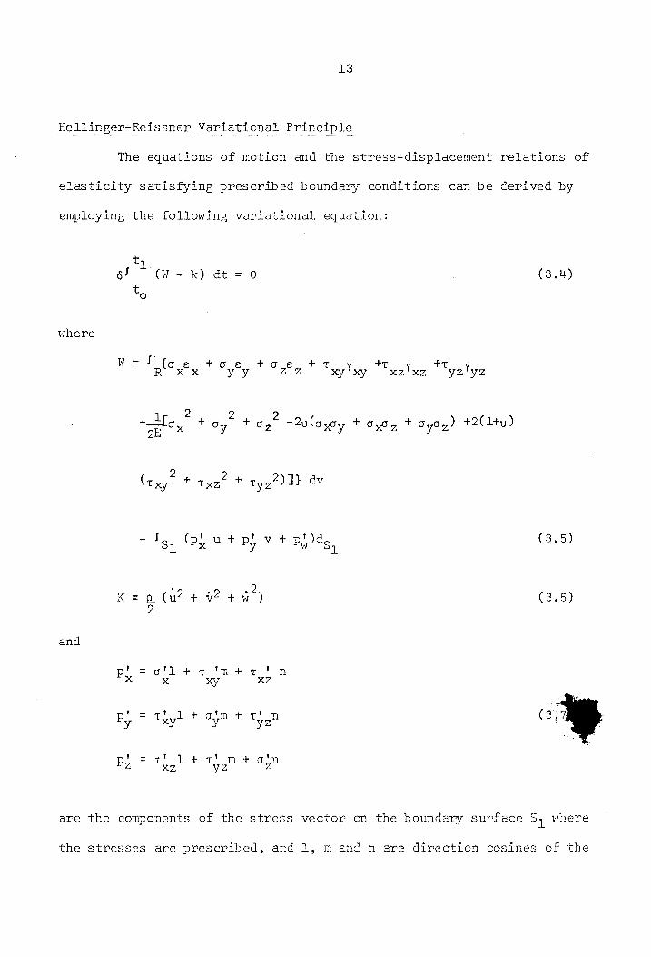
Hellinger-Reissner Variational Principle
The equations of motion and the stress~displacement relations of
elasticity satisfying prescribed boundary conditions can be derived by
employing the following variational equation:
t
éf t (W-k) dt = 0 | (3.4)
to
where
We J + + + , + , + nit Ey Oye FOE t Ty TT olys Myztyz
_ilr. 2 2 2 Hox + Oy + om -2ula yy + O50 5 + CySy) +2(1ty)
Ce sep 2)}} 4 Txy + TRY, + Tyz } Vv
-Jo (plhutptvtp!)d (3.5) Sy Py ¥ Py Py? Sy
. . 2 K = g (ut +024) (3.6)
and
t = 1 + 1 + ? Py. ot Ty TL n
Py = Thyl + ajm + Thon
tr - ~f ! t Po Tot + Tm + on
are the components of the stress vector on the boundary surface S, where
the stresses are prescribed, and 1, m and n are direction cosines of the

L4
outer unit normal vector. The body forces are neglected in the deriva-
tion. That part of the boundary surface S. where the displacements are
prescribed does not enter into the equation since the variation of the
known displacements vanishes there. The boundary conditions on either
displacements or stress resultants arise from this principle also. For
plate bending and extension, the surface integral term in the equation
(3.5) becomes
+ {J B h 1g * Us foo, ys - 3) ~J ' ' t , (piu + PyV + piw)ds :
LE
B h B h + Tus Ys >) + T zulss Ys - a
y
Fg. lagu, y; 3) + tux, Y> 2) + Tavs Y >» ay} dxdy
where SuR is that part of the edge surface on which the stresses are
prescribed; and Sar and Sip are those portions of the top and bottom
surfaces, respectively, where the stresses are prescribed. Substituting
the stress components from equation (3.3) and strains from equation (3.1)
into equation (3.4) and employing standard techniques from the calculus
of variationals, the following equation is obtained.
uy OP oP ey . oP ey oP, s ¢ g (l- 4 - a - 8, + ehul Su + [- 5 - 3 > Spt phvdov
° x y x y
qV 9V - x y —~— =
+ ee, Pi [ 5 5 S. + ohw]é w
x y

A
OM aM n+ 2 . x 323 too, YI -
+ L ~ qo oa y +-V = = & + an a | 6a Ox oy a 2. LZ
oM OM ho +t 3 T oA y X h oh aN iva. +E -— et - 2+ y - 250+ Fe) 63 + pee SK SE)
Ox oy y 2 y 2 Ox dy Gh xy
— Pp uP ou K vy v + vA - _ voh” ° [Pet et St ee OS + $ -— él ox Eh Eh 2E “2 12s (Sx yay? jor YI O,,
— P uP ov y 4 v + uh - ~ veoh i
+ aT OD = ft oo S te 5 - TT 6P dy Eh Eh 2b 12h ( XX y 59? 12a : 4
30, 12 12vu 60g U + + vo + [-- - = Mot = M —=— S — (S$ + - => pul 6 lox 7 no“, * Fs y ) Ben oe * tor Ox,x voy gp Pwd OM,
3 12 12v ss, uD - + + + (8-1 y = oe —-- (S +S _) oy 3 ¥y 3 x oh Z LOE NX 3¥
Eh E Y
ae
“. —~ 6V 5 _ _v url Oit 30 a6 _ 12 MM NM no OW _ a 24 VW
4 pt ay aa c es ao ] 614 + [ ' ry mt 4 or ry ed § ¥
SE y oy ou Gn? XY XY OX 50 LOG % 1.
+
—~ 6V 5 3 aw V r ae a 3 9... oh -_ _
+ [2 + aT OT OF; < r — ay + ae _ Q HS + ra ~ Cs + S
oy OA LOG ¥ 22, 70 Z 210 xX Yo¥
2,3 0... “ 3 i “ oh Zz i - . 1 oh” srt oh an ~
- -Wo=- >up (B wot Se LS S Tos © 7 pte UA FBT Ow + be Cig 82 * go age F Sy yy?
2,9 we 2 - “ 3 p a von oh 4
- -—=-— (P +P sa yléy; ddd 60. * (Pt PD = tpn viby edd,
t L - ' __ . t _ { oT
+ J> Fo {fp - PL) 6a + Gi - BN )éole + CCP - P+) bu + C x x x x xy XY
oO 1
! . . t _ 1 _
+ (4 - Su amc EoD - bP ) évo+ CM - 6 BAL RY ny eA KY KY A

16
2 _ t — _ xt _owlyan he - 1
+ [(P, ey év + Cn My 6B ]m + Cv, V dw + 1D (Sy S or iz
2 + [WV v') owt (ST S'-)éy]m 4C_dt yo ty? SWF ag Sy 7 Py PEF 1
ty a _ _ +i° Ff {[péu t+ M, sale +(P S6u+M 6alm+ (Pov +M dp]
tT. Co XY xy xy xy
— — he — n° + [{P 6v +M 68jm + [V_6w + — S™ 6y]J2 + LV 6wt+—S 6yJm
y y x 12 & y 12 y
} de,dt
j Le 3 2 o oh? 2,3 + 2 + {—f—poh* Ss, +82 (st 4 gt . 8 -~—=vp (MM +M S 2B 70 Z "910 22 4X Sry 105 W 5 o ¢ x yl
“tt — tL Sw } d,.dy t
Oo
. 3 2.3 ~ 5 ¢ 4 p98 on? g- 4 OR gt Foy ph Se 2
s ‘de °70 8? Sz * ai9 $ xx Soy los OUST
e ° t
(M +M )] éwh ~ did x Vy to a ¥
5, l cph? ph 215 uph* t+. {= [5— st+oi(ss +57 )-f2 yy - Sh’ (pl +P) S “2B “12 Z 60 ox VV 60 6 * y
3 . h t - pr y]sy} 1 did
12 to *Y
3. . . 2.5 2 1 uy - h , ~f t2 eh st 4 ph’ (gs +s7 )- oh yo - 2 (p +P) S 2E 12 “2 & X4X Yo¥ 60 6 x y

3 t h . 1 . Pe d
12 yey) xty
eo BL 3 - Qe [TphCudu + vov + wow) + ph*
- 12 (60 + BSB + yoy)” 0 (3.8)
The line integral involving Cc, is taken over boundary where the stresses
are prescribed, and the one involving C., is taken over the remaining
portion of the boundary where the displacements are prescribed.
equation (3.8), the coefficients of each variations must vanish
individually.
Equations of Motion
From the first five brackets of equation (3.8) arise five equations
of motion
OP.. oP - X+— 4085 = phu
OX oy
3P 9P ——a3L ~~ =s 3X + yt y oh v
JV aV
—%+—L+s5> = phw
M OM, + 3 xy - Ve + 2
Ox ay 2
ah oM xy y h
- Vl eee —
(3.9)
18
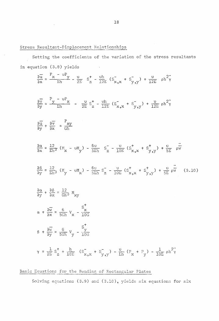
Stress Resultant-Displacement Relationships
Setting the coefficients of the variation of the stress resultants
in equation (3.8) yields
pu Px 7 UP U + uh - - v 2" ox Eh ~ OF °s ~ 138 (Sox r Sy? r L2E phy
—- P - vP ov. OY x Vv ot uh - v 2. by SCE DE 8s 7 TOE “Syn t Syiy? * Toe OP Y
du, av _ xy oy ax Gh
aa _ 12 6uU - Vv + + v _—
x Ens My W uM.) - ben 82 7 tor Sxyx * Say? Top PW
0B _ 12 ro 6u - U ot + v= ay ~ End “My ~ UML) ~ cep 8, 7 Tow ‘x,x t Sy,y? F spew (-10)
da, 2B _ 12 ay * ox Gh ey
+
oe HL By ax 5Gh x 106
+
— S ow _ 6 y
P+ ay * sch ‘y 7 toa
Ll ot h - - U 1 2. = SS ——~ -_ — - —__
Y= oe 8, tor “yon t yyy? 7 EW Ox t Py) > Top eh Y
Basic Equations for the Bending of Rectangular Plates
Solving equations (3.9) and (3.10), yields six equations for six

19
unknowns , Ws V,V,M 4M and M.. They are x° oy x XY y
DV w = S -k v7(S7) - Sh (2 v° st + 2 yest) - phw Z Z 1 Ox y
2 Xx oy
17-6 3.222 ph? wt “+ ph? uit * Sotisuy PP YW + T50g “Sy,x * Sy.y? * Tow 68, 7 ObY ?
+ 2st 4 st 2 XX Y oy
2 2 2 h* 2 _ phe * 3 2 ho+ he 1_- to” ‘x7 ‘e = too Ye Pa YM oo t Te T%:,x
3 3 3 k + h + h 1 + il ph = + —h —__ —_ - oY
12 Oe RX 120 ee yy * [30 I-v Sy Ay 60 i-v “°*
_ oh? ot
120G x
2 2 2 h* _2 oh* * 9 2- hot hey 1 To Vv vy - Vy 0G vy + Da Vow - a Sy + To Tou Oy
3 3 3 k + h + h 1 + ll ph —
r vie So yy * 730 Oo Axx * [30 Tu Sx xy ~ 60 Inv “oY
_ phe gt 120 “y
_ 6 l-v — _ 3U - 2-v Qt v +
M = DLS am Vay 7 Owexx + UWsyW) - cap 8, - a9g xox 7 BOG “yoy
ve ony

20
ch? 6 i ot +
- 2 OG x xy 12 Sth Voy + Vv x w,xy i Xs yx) J
6 l-v — — 3u - 2-v ot
= LE Ga - <—s -S My Lee Vyoy (ws + Ws.) - tah S 7 Boe Sy.y
18) + LL VU 3—
- p06 8x,x1 * GO Toy OF
3 2
where D = Boh and k = bo 2-0 The boundary conditions for this 1 (1-07) 10 I-v
problem are also obtained from the variational equation (3.8). Ona
straight edge of constant x, these are
Vo=zvi or weH=w X x
M =M! or a=a'! x xX
= t = t May My or 8 8
Whereas on a straight edge of constant y, the boundary conditions are
w'! V V' or w tt
y
M = M' or 8 = Bi y¥ ¥
M = Mi or a= a! xy xy
Thus three boundary conditions must be satisfied on an edge instead of
two as in the classical theory.
Governing Equations for the Extension of Plates
From the first three equations ot (3.10) and the first two equations
of (3.9), proper manipulation gives two equations on u and v and three
equations for the loads in terms of the displacements u and v. These arc

21
aa, OF OF aa, av - =~ CL 7+ Yeggy 7 (2 tv) gl t Gh (> + Say? + Sy = ehe
aX oy
2— 2— 2— 2— av au oF av au - xs
c[—~ + v-—— - (1 + vv) =] + Gh (Se + eS) t+ Ss = phv ay? dx0Y ox 3x2 dxoy y
_ 4p ou ov P= Cla + X35 - (1 + v)F]
P= of 8% + yee - (1 + v)FI y oy Ox
_ du av. Py = Choa + ox
_ Eh _ vot uh - - U 2. where C = oe and F = aE S IDE (Sox + Soy? i5E oh y
The boundary conditions for this problem, for rectangular plates,
are
a) ona straight edge of constant x
b) ona straight edge of constant y
P =Pt orue=iu xy xy
it <I
P = Pt or Vv
The equation for y is shown in the last equation of (3.10).

22
From the last integral of equation (3.8), twelve initial conditions
arise. These may be initial displacements and initial velocities. For
the bending problem, there will be six conditions: two on w, two on a
and two on 8. There are also six conditions for the extension problem:
two on u, two on v and two on jy.
B. Cylindrical Bending of a two-ply Laminate
The derived governing equations for three-dimensional problem are
specialized to solve the two-dimensional problem. A two-ply laminate is
shown in Figure 2. A distributed load q(x) is applied at the top face.
Recognizing that almost any loading function can be expressed in the form
of Fourier series, a sinusoidal loading is used for q(x). The laminate
is simply supported at both ends and is in a state of plane strain with
respect to the xz plane.
The governing equations of a single ply of the laminate subjected
to static bending can be shown to be
- + _ 3+ div °2 oh ax k aS, kh Px at OD 2 dD 2 ip 33
+
~— ds aa _ 1L-v QTL vv ds. hu x
2 2Gh x 4G dx 24UG6 2 dx d
3 ds_ ae. __ dw ne awe | gt ok Se kx O- - ae 7 5-0) .3 Io "x BCh dx 10G 5

23
Figure 2,
. ot
3 ° 10 x 10° ksi
1/3
a
30 x 10° ksi
225
Aluminum-Steel Laminate in Cylindrical Bending.

24.
— 2 Aas
~~. _v_ du + i i-2v ot 3-3v0-5v h x
Y° " Toy dx 4G d-v z B30E(1-v) dx (3.11)
- 2 +
ge pee 4h ot ye kn Sfx x 3 2 x dx 12 2
dx dx
+
ye pee ye Sx x 2 Z, 12 dx
dx
> - 2h a ph ov ot ht vu Bx x l-v dx 2 l-v Zz 12 l-v dx
All unknowns are expressed in terms of applied load q(x) at the top face
and the unknown interface stresses o and z. The interface stresses are
solved by the continuity conditions of displacement at the interface,
these are
ee ee 22, 1 2 1° #67°2 2
(3.12)
ae = Ww _ 2
1° > YY 9° 9 Yo
Recognizing that the boundary conditions of a simply-supported
laminate are w, Mand P, equal to zero and that the loading function q(x)
is in the form of a single sinusoidal function, the following forms of
the solutions of T and o are used
T = C. cos
0/33 > 2X
+c, (1 - =) 3 & (3.13)
o = C. sin —-—+C

25
Writing the equations (3.11) for each ply and applying the con-
tinuity conditions (3.12), it can be shown that C. and Ch are zero and
C, and C, are given by solution of the following simultaneous equations
2 9 2 ; ed P2, . no ; oP) . 1 hy C2 . 3-30) -5v,
2D,” By 10° G, G, Wn 1-0, “4G, SE,
2 2 2 _ 1 hy, C2 . 3-3U5-5U, 4
lin I-v; ‘4G, SE,
k k 1-v 1l-v 1 14 1 2. 2 1 2 + Cif (—— + —)n° + (— + —)n + = h h 2°D, ” By Bb)” By 86, 1" 8G, 2
_ nt Ky 5 1-v,
=a[p-+ p® - ge hol 2 2 2
1,2 yPz Pps g ty tr, Clase te > 2m (eat a! (8-28) 1 2 wy 2"9
ec tech - 22) BCh_ 22,-5 po “2_ in 22, 2°20" 6, 7 G, 2D, ~ Dy 2 Dd, 20 &,
where n = “ Once C, and C, are obtained, the displacements and stress i 2
resultants are solved by the following equations
h kh — ~-n 3 1 2 lol . 1X Wa = Dy [Cn + Cian + C, ky n+ Cy Tp! sin z
h kh - =n —, 3 2_2 — 2 2 -. TX We = D, [2 ~ q)n~ - Cnt (C, - qQ)k )n - Cia sin 7-
v l-v h uU_2 G. 3-3u_,-5u 2 C y 2 ctrectn- be. - Lb CE, 22 1) Ty cin
1 Go 12h, 4 2 6(1-v,) 4 ES 5 n R

HW H
Nn uv
26
2 - —~30_-5v lie Vo . 1-v, oe a- hy ee . Co 3-30,-5U,
G, 1 2h,, uy 2 6(1-v, ) 4 Ey 5
“1 Tsin ~ aa)
Lp eR 2 hk oy cog TE G Loh ~\o “yp # Olt 1 g 1 l
l-v hv 1 2 — 2°2 TX aa LCE n + (Cc, + q) n- Oh C.J Cos t
2 2
2 n° +c 1 n*-C os n- _ C_.lcos DL 1 "2D, 2 SGjh, 206, “1 2
3 h 3U Vv _— 2 2 — 2? 2 TX
[(q - C,) Boge. n* + (C, - q) === n - = -s CL] cos — 2° Dd, 1 2D, 2 56h, 206, “1 2
(3.15) TX
- C, n cos —
(C, -~q) ncos & R
h L 2 1X
- n(C,n + Cy 5) sin >—
—_ Ay TX n (ce, - q)n- ¢, 5] sin 5—
.. 7X C. n sin —
. 1 - C n sin

27
The displacement distributions and stress distributions for a section
are obtained by substituting equations (3.15) into (3.1) and (3.3),
respectively.
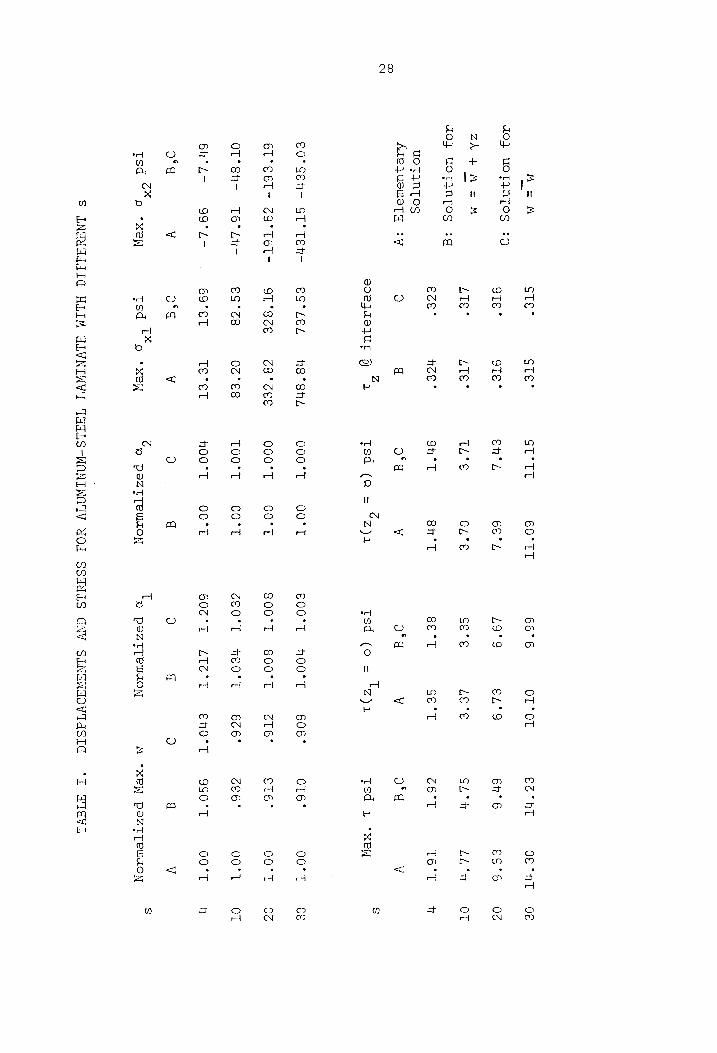
Examples and Discussion
Solution for the laminate as shown in Figure 2 are shown in Table I
for various s, which is the span-to-thickness ratio of the laminate.
Three cases are shown for comparison. Solution A is calculated by the
elementary beam theory in which the transformed section of the two
materials is used to calculate displacements and stresses. Solution B
is obtained in this study. In order to observe the significant effect
of the displacement function y, solution C is obtained by dropping y
in the expansion of vertical displacement w. The normalized maximum
vertical deflections are shown for the three cases. The solution B is
about 5.6% and the solution C is about 4.3% larger than the solution A
for s = 4. This indicates that both shear deformation and normal
straining should be considered in which s is less than 10. The normal-
ized horizontal rotations about y-axis Oy and a, are shown for solu-
tions B and C. In the beam theory, a is a constant through the
thickness. It is shown in the table that %® is not the same for each
layer, specially when s is less than 10. The solutions of the maximum
normal stress o.. at each layer are almost the same in three cases. The
maximum shearing stress are at the neutral axis for the solution A and
calculated at the interface for the solution B and C. In this example,
the neutral axis is located near the interface. The shearing stresses
at the three points of the cross-section are the same for both solutions
28
M=aiM
JOF UOTINTOS
:9
ZXQ+M=2—
M
OF
UOTAINTOS :gq
UOTANTOS
ALBLUSUSTY
sy
€O°SEh- ST*
Teh
6T°S6T- Z9°T6T-
OT’Sh- T6°Lh-
6h°L- =
99° L-
o*d V
tsd o%
5 *xey
STE°*
OTE °
LTE *
ECE”
U
Soe fASAUT
€S°LEL
QT *8ZE
€S9°%8
69°ST
afd
tsd T%
STEe*
OTE *
LTE*
HE *
n8 "StL
68° CEE
0Z°E8
Te *eT
V
*“ XP]
ST°TT
end
TL“€
n° T
000°T
Q00°T
TOO*T
n00°T
O
@
60° TT
66° 4
OLE
Bn T
00°T
QO°T
00°T
OO°T
q
0) PeSZTTEUaoNn
66°6 OT* OT
EO ° nT
O€ “AT
L9°9 eL°9
6° 6
ES*6
GEe°'e LEE
GL° ht
LL ‘t
BE°T Gert
C6°T T6°T
og V
of V
Tsd (0
= lzya
Tsd 1
*XeW
€00°T h00°T
606° OT6*
00°T
800°T
800°T
cL6° eT6°
. OO°T
ceO°T heo°Tt
626° CoB"
0O0°T
600°T LTé°T
e€nO0°T 9S0°T
00°T
0 q
O d
V
+ 0 peZTTeUdoy
M *XPY
POZTTeUToN
S INFeaIIIG
HLIM
ALVNIWVT
TSRLS-WANIWATV
YOU SSaeYLS
ANV SLNENSOVTdSIG
“I d1avVL
Of
OZ
OT
O¢
O%
OT

29
Band C. This is also for the normal stress c. at the interface.
In Figure 3, an example is shown where the neutral axis is not near
the interface. Comparison with the solution of the elementary beam
theory shows excellent agreement for the maximum normal stresses and
shearing stress for s = 10. Thus it is natural to conclude that the
theory developed with linear terms in the expansion of the displacement
functions is good for the isotropic, homogeneous ply in the laminate.
Fourier Series Representation for a Uniform Load
The Fourier series representation for a uniform load q is the
following
_ Ag TX 37x , 1 OTX q(x) = 7 [sin q + 3 sin => 5 n> + -~--]
or
bg , q(x) = -2 og 4 sin BU (3.16) T n R
n=1,3,
The partial loads represented by the first three terms are shown in
Figure 4(a), 4(b) and 4(c). The sum of the first and second term is
shown in Figure 4(d), and the sum of the first three terms is repre-
sented in Figure 4(e). The sum of all the terms of the series gives
the straight line q = 1. In general, only the first few terms of this
series are needed to achieve sufficient accuracy.
The laminate as shown in Figure 2 is solved by two Fourier series
representations of the uniform load q = 1 for s = 10. Solution for
stresses and displacement distributions are shown in Table II. Three
cases are shown for comparison. Solution A is obtained by using only
the first three partial loads. Solution B is obtained by using the

30
Oo") Al.
Er | [ +
N |
{ N w | r
& 2D
ASL as -~-.8 -.4 Na J L ! i. —L4 ab. 1 1 J t i J
L450 452 4 .usts 107! ~.6 -.2 2 Ns x 107°
wl) u(L)
NA.
1. 2. a, De -50 -25 50 75 100
4 Figure 3. Displacement and Stress Distributions for Aluninum-Steel t
Laminate, h, = .1", h, = .5", s = 10 1

Pigure 4,
31
TM
a+
tA
pee
mw
Fourier Series Expansion for Unifor
(e)
a /4

32
60%
T_I* ox
Tx %
ZO d+
Zo Gt"
Wt Wt
Wo xy
604° OTL"
este" TSTe*
et A
Ag
Q9T6Z° STLZ°
9TLe" 6TE0°
STEO"
G2T°T g92T'T
LZT'T S°T
tht ont
769%" = 697"
661S°- 661S*~
O xd
eV oO
4d uV
oO q
V qd
V
dry (2/8) W
Ut/x (4)
“A ‘UE
| OT x
(Z/4)M ‘UT
7-01 ¥
(3)n
0 0
0 0
0 GO"ZOT
ZL°TOT Z6°TOT
Tot’ LOT’
6Z°S 60°S
6th
nee’ TSE"
Li’h 6T°L
86°9
g6S* €29°
ST'L §©6©98°9)
so L9*9)s EEG
QZ*OT)— HZ
OT
uotintos AdejusueTg
+9 ces’
= g98°
Te°s 99°S
TTh'S TTS
the ene
sotdes detanoj
swie, g
gq 666°
8se0'T chee
=o LZ" OBTE
SeTies detTdnoj
slide} g
iV €90°T
€0T‘T 0
0 0
OT'6S- ZH°6S-
0S°6S-
q V
3 q
V 2
q Vv
TSY (Z/%)"0
Tsy (t)2
TSY (Z/%)" 2
ror =
8 fue
= Su
fate =
fy ey
T =
b qvoOT
WHOJINA V
OI NOLLVINGSTYdTY
SAYS
aqaTdNoOd AG
GLVNIWNVT
THSLS-WONIWNIV
YOd SNOLLAGLIeLSIG
LNAWSOVIdSId
ANV SSaeaLS
“IL aATavL

33
first five terms partial loads. Solution C is calculated by the
elementary beam theory by using the transformed section. The stress
C, is shown for mid span at the top face, interface and bottom face.
Two values are shown at the interface, since the elasticity moduli
are different. Solution for OL. is good compared with the elementary
solution even only three terms are used. The shear stress resultant
for the solution B is better than the solution A compared with the
solution C. Therefore the distribution of Te is the same. This
indicates that in order to obtain a better solution for TL» more terms
in the series be used. The solutions for displacement u and w are
good for the solution A. The maximum value for w is occurred at the
interface. The normal stress o. for the solution B is better than the
solution A at the midspan, while it is zero at the supported edges by
the Fourier analysis.
The displacements and stresses along the interface for this problem
are shown in Table III for solutions A and B. The displacements u and
w are the same for solutions A and B along the x-direction. The
stresses TW? oO, and Vy from the solution B is better than the solution
A. The stress Oy My and P are good already from the solution A.
Thus, more terms are needed in the solution of shearing stress and
normal stress Oo. by a Fourier series representation of the uniform load
than the normal stress OL. and displacements u and w.
In general, for a N-ply laminate, there are (N - 1) sets of
equations (3.14) obtained from the displacement continuity conditions
at the (N - 1) interfaces. The solutions of the interface stresses

34
66S°S 809°S SéT*T Lot’
HEE
* TS¢°-
6eh*o~ 92°
OT Ion"
E- 4G
°OT CLE" CLE"
c/%
Bens
ben TS
E60°T €60°T eS"
99¢° 86d
°- ne?
LG0°T 966° T
See E=
9T6* 6
Lee" e-
LE6*6 €9S °
690° 080° 080°
cT/%S
LLo°n T96°h 000°T L66° Soh°
Lot" 8ce"- hice
nSh* %
OLn'S 8TO*E-
0S0°6 8EO°E-
0€0°6 9ES" SES" SST° SST°
€/%
Lot*h HOG" h
nhs *
St °
8SZ" OEL° TTE* -
CCE’ =
OLL*E
6T9°E 66m"
o>
L£nG*L Oot
o-
LEG*L Tot *
noc’
Tad"
Tod"
n/%
TIL‘’€
6cT’°€S
Géo93°
8d9"
686°
TLO'T
LOE'
E8Et
806°h
oc0°s
dah’ To
Ogu’ Ss
cEeL*T-
69n's
BET’
SET"
ELC*
ELS"
9/%
STL T
769° T
HE *
One”
990°T
eBe°T
Bice ~
986° ~
LO2°9
68E°S9
Gig
*
TH6'S
TL8*
CO8°S
oL0°*
oL0°
LOE *
LOE*
CL/S
0 q
0 V
0 q
0 v
Boh’ T q
666°T V
0 g
0 v
ZBL
d 086°9
¥ 0
‘TY otis
© 0
*TY orig
= =¥
0 g
0 v
ete" q
Te" v
0
oT =
Ss *"/x
T =
b CYOT
WHOJINN V
YO4 SAIYSS
USTUNOI A
GLVNINVI TGGLS-WANIWNIV
YOI JOVSINALNI
SHL SNOIV
SASSTYLS ANY
SLNENAOVIdSIG ‘III
Favs

35
are solved once the properties of each lamina and the dimensions of the
laminate are known. With the displacement and stress equations, the
stress and displacement for any point in a laminate are obtained. The
formulation described in sections III-A and III-B can be expanded to
solve the general anisotropic laminate. Since the formulation is
lengthy and restricted to the special ease of boundary shape of
composites, the numerical analysis, the finite element method, will be
used to solve the linear elastic, nonhomogeneous, anisotropic laminated
composites with boundaries of arbitrary shape.

IV. FINITE ELEMENTS IN TWO DIMENSIONS
An analysis of a laminated plate by discrete elements connected
at a finite number of nodal points can be performed by using a direct
stiffness or displacement formulation. Solutions to the fundamental
equation of the linear theory for laminated composites, which was de-
scribed in Chapter III, will be obtained using this approach. In this
chapter, a 16-DOF element and a 24-DOF element will be developed for
the two-dimensional analysis of laminated composites with various
loading and boundary conditions.
A. 16-DOF Element Formulation
For the analysis of arbitrary laminated anisotropic plates, a
rectangular plate element shown in Figure 5 with 2-fOF at each nodal
point will be used. This element will perform the deformation with a
cubic expansion in the x-direction and with a linear variation in the
z-direction. The deformation pattern for the displacement corresponds
to the linear theory described in Chapter III. The solution accuracy
of the displacement formulation depends on the ability of the assumed
functions to accurately model the deformation modes of the composite.
In selecting this element, a cubic deformation pattern for the displace-~
ment w is assumed and for most loading conditions this will give the
correct solution and there is no need to have many divisions in the
x-direction.
36

37
5 6 7 8 Zz A ~
[ | |< 52 < >
b —O ——o— 1 2 3 4
i 3 3 i 8 8 8 8
— D. D —
Py
1
L L g
3 3 3 P P
1 2 z= Py
; *
\ Normalized Trace
\ |
\ 2. 7
NS . oe
i \ | } ! J —l A/c
.2 3 «4H 5.6 1 2 3. 4 6 10
Figure 5 Oixteen DOF Rlement, Distributed Force and Trace.

38
Displacement Functions
The assumed displacement functions associated with the degrees
of freedom shown in Figure 5 are
2 3 2 3 t+ oa,X t+ a,2 t+ a,% + a_Xz + a.X +a_,xX Zt aX 2 u=a
1 2 3 ly 5 6 7 8 (4)
wt + + +t x? + xXxZ + xo +a oe ~ Gg T Gy gk T O44 T Oy 5 O13 Cay 15
3 + O16% Z
or in matrix form
fu} = {[M] {a} (4,2)
where [MJ] is a function of x and z. The sixteen constants {a} are
evaluated by solving the two sets of eight simultaneous equations which
result when the nodal coordinates and the corresponding nodal displace~
ments are inserted into equations (4.1). Expressing {a} in terms of the
nodal displacements {u,} which are now the unknowns of the problem, if
the inverse of [A] exists,
[A] fa} (4,3)
-1
ay
G fe ue it
fa} = [A] ~ {u,} (4,4)
where [A] is the matrix relating the nodal displacements and the con-
stants fo}. If cay+ does not exist, then different displacement

39
functions must be chosen. The displacements for any point in the element
are obtained by substituting {a} in equation (4.4) into equation (4.2),
thus
{uk = [mM] cay? (u,} = EN] {u,} (1.5)
where [N] are shape functions such that Ny = 1 at node i and is equal to
zero at all other nodes. It defines the deformation of any point in terms
of the nodal displacements.
Derivation of Element Stiffness Matrix
With the displacement functions formulated, the strains are cal-
culated from equations (4.5) and expressed in terms of the nodal dis-
placements. This is done by appropriate differentiation of LM], which
yields
ex] f ae | xX
Es - O49 ~1
fe} = | se | = EQIAl “fu,} = [Blt{u,} (4,6)
+ du | OW
| “2 oz Ox
where [Q] is the differentiation of [M] and [B] is the differentiation
of [N]. The stresses are related to the strains by the following
equation

LO
{o} = |°z = [De} (4.7)
where [D] is the elasticity matrix. For the transversely isotropic com-
posite material [23] in a state of plane stress
Bu. Fay 31 0
P= Yip M37 FY y3'31
E [D] = 33 0 (4.8)
T= Mi gh 37
| ymmetry G13
and in a state of plane strain
; T= Vog% 39 . ¥37tP 91% 39 0 ul E hl p
[D] = BE. +7 ree oo (4.9) 33 —— + F
symmetry Si4 where F = (1 -v U_nU - Ul .UL AU ); and 1, 12°21 "23°32 ~ “13"31 ~ “19%23"31 ~ Yoi%13"32 2 and 3 refer to the principal directions of the lamina, and V43 is the
Poisson ratio measuring normal strain in the 3-direction due to uniaxial

ui
normal stress in the l-direction. In this study the axes of elastic
symmetry of the various layers are parallel to the structure axes. The
inclusion of anisotropic properties for composite material applications
is readily accomplished at the dement level by inserting elastic con-
stants associated with the principal directions of the composite.
Thus, with the displacement functions in equation (4.5) and the
elasticity matrix in equation (4.8) or (4.9), the element stiffness
matrix is formulated straightforwardly by the following equation
[k] = J [BJ (DICBlav (4,10)
This element stiffness matrix relates the nodal displacements fu, } di-
rectly to the nodal forces {£3 by
{f,} = [k] fu, } (4.121)
As shown, the element stiffness matrix can be determined by a series of
systematic steps in matrix algebra based on assumed displacement
functions and known material properties. The more realistic the dis-
placement function, the closer the stiffness will be to the true value.
Consistent Element Joint Loads
The nodal forces due to the distributed force as shown in
Figure 5 are calculated by the following equation
S Sésuds = 12 ,pouds Pjéu, + P6u, + P,6u,, + Ps uw, (4,12)

42
where p is the load intensity; Po» Pos P, and Py are equivalent joint
leads; and Uy» Us Us and uy, are joint displacements. With Figure 5, it
can be shown that
— 11,x x2. 9,x,3, — x, 45x, 2 p= fi - sp) + SF) - ay? ] Py + [o(F) - >)
+ Fey 5 + FSG) + 1B, + HE - 3° (4.13)
where Py Pos Py and Py are load intensity at node 1, 2, 3 and 4, re-
spectively. Similarly, u can be expressed in terms of u Un» Ug and u 1?
with the same form. Substituting equation (4.13) into the left side of
uu
equation (4.12) and integrating the consistent joint loads coefficients
become
— Q _ “T — im
[P| 128 ge 36 19 Py
P, 2 99 = 648 ~81 -36 Py _ = T6505 | = £P]{p} (4.14)
P ~36 -81 648 99 D 3 3
P 19-36 99 128 D a i | LP For a uniformly distributed load, the coefficients are shown in the top
of Figure 5(b).
Trace of the Flement Stiffness Matrix
The trace of the clement stiffness matrix, which is the sum of
the diagonal terms in the matrix, provides a convenient measure of the

Ng
quality of the element [20]. The best element of a group of elements
having the same geometry and desrees of freedom is, in general, the one
with the lowest trace. The trace of each 16-DOF rectangular element
with various aspect ratios of A and C but with constant area, equal to
AC, is shown in Figure 5. Evidently, the best one has an aspect ratio
located between 3 and 4, but an element with aspect ratios from 1 to 10
will perform very well. This provides a guide for selecting an ideali-
zation of the structure by recommending that relatively thin elements
should be used.
Assembly and Analysis
Beginning with the idealization of the structure and the assumed
displacement functions, followed by the formulation of element stiffness
matrix and joint loads, the last step involved in every finite-element
analysis is the summation of equation (4.11) over all the elements in
the structure. This result can be writtcn as follows
{F} = [k] {u} (4.15)
where {F} is the load vector due to the external forces including con-
centrated and distributed loads; [k] is the structure stiffness matrix,
and {u} is the unknown nodal displacement vector. The nodal displace-
ments can be determined by solving the system of simultaneous equations
(4,15).
With the displacements known, the stresses can be calculated by
equations (4.7) and (4.6), which give
Hu
{o} = [DILBI{u,} (4.16)
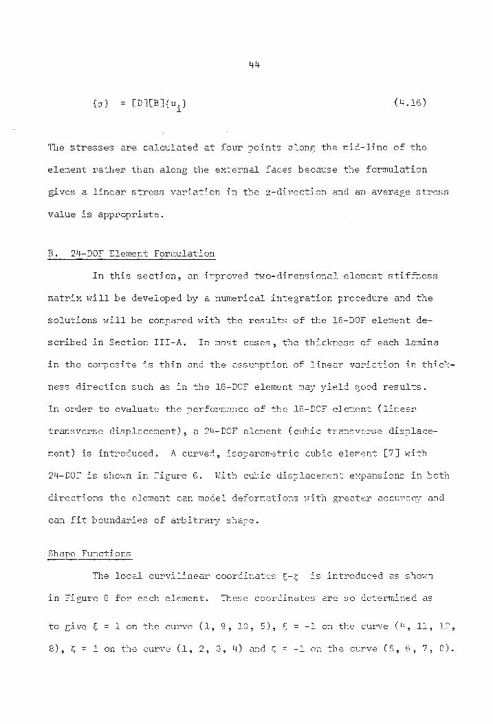
The stresses are calculated at four points along the mid-line of the
element rather than along the external faces because the formulation
gives a linear stress variation in the z-direction and an average stress
value is appropriate.
B. 24~DOF Element Formulation
In this section, an improved two-dimensional element stiffness
matrix will be developed by a numerical integration procedure and the
solutions will be compared with the results of the 16-DOF element de-
seribed in Section III-A. In most cases, the thickness of each lamina
in the composite is thin and the assumption of linear variation in thick-
ness direction such as in the 16-DOF element may yield good results.
In order to evaluate the performance of the 16-DOF element (linear
transverse displacement), a 24-DOF element (cubic transverse displace-
ment) is introduced. A curved, isoparametric cubic element [7] with
24-DOF is shown in Figure 6. With cubic displacement expansions in both
directions the element can model deformations with greater accuracy and
can fit boundaries of arbitrary shape.
Shape Functions
The local curvilinear coordinates —-c is introduced as shown
in Figure 6 for each element. These coordinates are so determined as
to give € = 1 on the curve (1, 9, 10, 5), € = -1 on the curve (4, 11, 12,
8), © = 1 on the curve (1, 2, 3, 4) and ft = -1 on the curve (5, 6, 7, ©).

x
E = ,33998 H, = .84785
He, = .,65214
gE = -,86113 86113) Ly 3 2
0 Ay Ay
c r= -.33998
Co
Cy
ay a, a, ay
Normalized Se - Trace
uy, a
1 2 3. 4 6 10 A/C
—t * ry, slags Tm i TO re ey ee ~ . - aes to Figure 6. Twenty-four DOF Plement, 4 x 4 Gauss Rule and Trace. t
46
The relationships between the Cartesian and local coordinates are
2 2 3 2 xX = a + a6 + O 5 + O 6 + O90 + OG + O 6 + O46 0
+ ago + ioe + 36° + O18 2° (4.17)
Zz = same form
or in matrix form
{x}. = [M]to} (4.18)
Substituting the corresponding nodal coordinates in the two systems for
each node results in
{x,} = [Alf{a} (4.19)
Solving the above equation yields
fo} = [AY “{x,} (4,20)
Equations (4.19) and (4.20) are similar to equations (4.3) and (4.4),
Substituting equation (4.20) intu equation (4.18) gives
T x = Nx. + Nix. +... + N..x.. = {NO f{x.}
Li 2 2 12 12 1 (4,22)
T = y t eo a 6 t = e Zz Nj, + NZ. + + Ny 249 {nN} tz, }

47
where N. are shape functions and are functions of & andz [7]. They
have a value of unity at the point in question and zero elsewhere. It
is a most convenient method to establish the coordinate transformation
by using these shape functions. The twelve shape functions are shown
in Appendix A for the 24-DOF element.
The displacement functions can also be defined by N, such that
u (Et) = Nou. + Nout... tN tn} fu, } 144 a, 12°12
(4,22)
w (&,0) H Hi N.w. + Nw. + T t T 1 5 wee + Noy {Nn} tw, }
Since the shape functions N. defining geometry (4.21) and functions
(4.22) are the same, the elements are called isoparametric [6].
Coordinate Transformation
As shown in equations (4.6) and (4.10), the differentiation and
the integration are taken with respect to slobal coordinates x-z, but
the N. and integrand are functions of € and t. It is necessary to ex-
press the global derivatives in terms of local derivatives and to carry
out the integration over the element surface in terms of the local co-
ordinates with an appropriate change of limits of integration. For
derivatives of Nes we have
5
ON O 3 ON oN,
st meas 2 _— i
= = [J] (4.23) oN 3 3 oN oN,
1 _* _e@ J 1
oc at, af OZ ag,
48
where [J] is the Jacobian Matrix. The global derivatives become
oN. | aN,
ox -1 J€
= [J] (4,24)
oN. oN.
az | | 8c | where coyt is the inverse of [J].
For isoparametric formulation, [J] is
aN, ON, | ON XB) ey:
[gy] = 5 4 = [C][xzZ] (4,25)
J T
oN, OM. Bae to, dn COL dC xe
; | M12 722] where [C] is the matrix for derivatives of Ne with respect tof and z,
shown in Appendix A, and [XZ] is the element global coordinate matrix.
The transformation of variables in the surface integration is
dxdz = |J| dé dz (4.26)
where | o| is the determinant of [J]. The region with respect to the
integration can be written as
sl sl SCF r yy Hy Ly ShE 26) dE de (4.27)

4g
where G(&,c) stands for [By EDIE} 3] ; [B] is shown in Appendix A and
[D] is the same elasticity matrix as given in Section A.
Element Stiffness Matrix
The formulation of the element stiffness matrix, equation (4.10),
can be rewritten as
- S cay! - Jt fst Ck] = “ [BJ CDI[B]dv = 7, 15 Gle.c)de dz (4,28)
Due to the tay matrix, in which polynomials occur in the denominator,
the above integration is carried out by numerical procedures.
The location of the sixteen Gaussian points (a, C3) and the
corresponding weighting coefficients He for the 4 x 4 Gauss Rule is
shown in Figure 6. Equation (4.28) then becomes
[k] = i # H. H. Gla., c.) (4,29) isl jel * td
Trace of the Stiffness Matrix
The trace of the 2H-DOF element stiffness matrix is shown in
Figure 6 for various aspect ratios A/C with constant element area.
This comparison is for rectangular elements. As expected, the lowest
trace is for the element which is square since the element is cubic in
both directions. The curve is symmetric with respect to the lowest
value of the trace.

50
Consistent Element Joint Loads
A cubic curve and its curvilinear and cartesian coordinates
with shape functions are shown in Figure 7. The following relationships
exist
u= Nvu Li
nd
p iPs
x = Nx, 11
(4.30)
The element consistent joint loads equation (4.12) can be written as
{Su }'{p} = foul! SP (hte)? Cedtwt? (pt ae
or = {PE = FF twitch” Gon? GB) ae
where C. = N, .. Consider the element P,_., it will be 1 1,4 11
~l 537 -3 139
P1127 03 Tio Te Fae] 1*
. T L 2b Setting {x}° = [ 0 5 = U1, P,, becomes
— 537. L 3 | 2b, 139 _ 8b
11°” «61120 3 16 3 3360 ~ 105
7 oe a gk This is equal to Pal
Psy can be obtained from equation (4.31).
(4,31)
in equation (4.14). Similarly, other elements of

n= h¢ (ge. levge - one? + 1) LE 1- €)(9—& - 1) Cc. - TE 18— - 278 + 1
N J ; Soe ) ty = 7a ~ 3E)(1 - &— ) C, = Tet 9s -~2& ~ 3
g 2 9 2 , = E ~_ = - 9 - N., we + 3E)C1 ro) C. a3 E 2e )
1 = ly (or lero eR oT ES = = QF ne 2 ~ Ny = yeti + 098 - 1) C, = pet® 6 + 27 8 - 1)
(p 7 T wT 7 - . To TT
“4 1 x | Py
Py a Ne Xe P.
= r Cc Y i 1 oN __ aE pof = -1 far, | Ea So Sa Sut fe | a Mo Ma MA fa] 3 3 3 3
D . _
u Pa | Au | | Pa |
Figure 7, Consistent Element Joint Leads for Cubic Curve Line.

52
Stress Analysis
Following the standard procedure to solve the unknown nodal
displacements, the stresses are calculated by equation (4.16) at twelve
nodal points on the edges of the element. This time the local coordi-
nates §€ and =f are used.
C. Applications and Discussion
Three problems are analyzed by computer programs for the 16-DOF
and the 24-DOF elements. The framework of the programs was taken from
an existing program for rectangular elements with 8-DOF [24J, in which
the element stiffness matrix was formulated directly like the one for
16-DOF in this study; and from a general quadrilateral program with
8-DOF [25], in which numerical intepration was used to formulate the
element stiffness matrix like the one for 24-DOF in this study. For
analyzing the transversely isotropic laminated composite, the element
elasticity [D] subroutine was also modified.
This example was solved in Chapter III by the analytical method,
in which the linear expansion of displacemes.t functions are assiied,
exactly for the sinusoidal load and approximately for the uniform load
using a Fourler series expansion. The idealization of FEM analysis for
16-DOF and 24-DOF rectangular elements is shown in Figure 8 for the
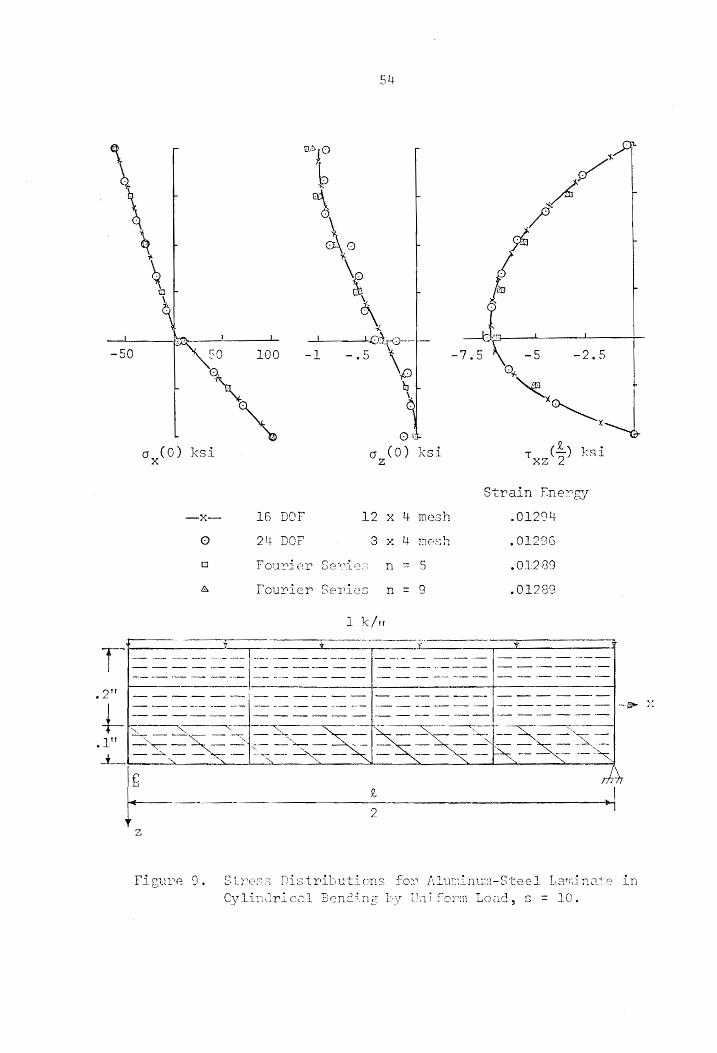
Sinusoidal load and in Figure 9 for the uniform load. The uniform mesh
of 3 x 4 for 2H-DOP element and 12 x 4 for 16-DOF element is employed.
Each of the 24-DOF elements are sliced equally into four layers. Since

aD
-50
oO
Jor
25 75 50
(0) ksi x
Yo oO
7
Anal. Sol,
16-
244--DOF
DOF
53
oO
0 =o T
XZ (>) 5 ksi
Strain Energy
007563
.007988
2007973
ee Ne ee
Xx NN MoT Boo
a= SaaS} TSE aE SSSee=
SESCES/ESSS NY SESE
fh
in Cylir
Stress -_
rd x ae teal
Distributions rn rend 3 ne
fer Aluminum-Steel Laminate
Ty Sinusoidal ads 'y Sinusoidal Lead, s 10.
-50
L. 16 DOF
24 DOP
1
Ot
(0) ksi
S
2
3.8
Q e =) k Tyo? KS
ers train En
201294
.012°6
a Fourier Sevinn n= 5 201289
Aa Fouricr Series n= 93 .012789
Lik/n
+7} ¥ + ¥ ¥
| ee ee eb ee ee Pe
Oe oe eo ee
| = ee — _— ~ were ee ee ae ene — — ——
a ae ee _—|— — — —N-— — — Ke
+ OTT aS a aN RO
E a
Db.
IN
Gt o> Figure 9, trons TY 7 ww ia} deo tribution
Wrage initio Pp aAtner Cylindrical Bending
for A . rt yay oT
i OL. CIM ua —
qt Ko
. . Tuminumn-Steel Lanminats
ad = aay S
~
LT

55
it is a symmetric problem, only the half span of plate is considered.
The aspect ratio A/C of each element is 3.75 for the 24-DOF element and
15 for the 16-DOF element. These are within the ideal range of the
trace as shown in Figures 5 and 6. The boundary conditions are zero
horizontal displacements at the center of the span and zero vertical
displacements at the support end. Since the solution for displacements
are in excellent agreement with the analytical solution, only the com-
parison of stress distributions are shown. Note that the stresses cal-
culated at the midpoint of the thickness for each element in 16-DOF,
where the displacements vary linearly in the thickness direction, are
fitted closely on the curves of the analytical solution. But in the
24-DOF element, stresses are evaluated at the nodal points along the
edges, a, and TL, are in good agreement with the analytical solution
and o. is not. o, can be improved by using a finer 3 x 8 mesh.
The strain energy for the three cases are also shown in the
Figures. Since no initial strains or initial stresses exist in this
example, by the principle of enerzy conservation, the strain energy will
be equal to the work done by the external loads which increase uniformly
q
from zero. Thus the strain energy for the analytical method, U = =:
For the finite element method [FEM], U = ful Ek Hul/2, as shown by
Zienkiewicz [19]. The larger the strain energy, the better the apprexi-
mate sclution. Generally use of a finer mesh will increase the strain
energy. From a3 x 4 mesh for the 24-DOF element and a 12 x 4 mesh for
the 16-DOP element, it appears that one 24-DOF element is better than
four 16-DOF elements for the Laminate with isotropic layers. Results
56
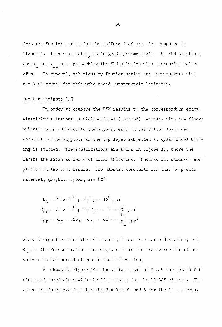
from the Fourier series for the uniform load are also compared in
Figure 9. It shows that o is in good agreement with the FEM solution,
and o. and TL, are approaching the FEM solution with increasing values
of n. In general, solutions by Fourier series are satisfactory with
n= 9 (5 terms; for this unbalanced, unsymmetric laminates.
Two-Ply Laminate [2]
In order to compare the FEM results to the corresponding exact
elasticity solutions, a bidirectional (coupled) laminate with the fibers
oriented perpendicular to the support ends in the bottom layer and
parallel to the supports in the top layer subjected to cylindrical bend-
ing is studied. The idealizations are shown in Figure 10, where the
layers are shown as being of equal thickness. Results for stresses are
plotted in the same figure. The elastic constants for this composite
material, graphite/epoxy, are [2]
6 ° 5 .
Ee = 25 x 10 psi, Ee = 10° psi
G = .5 xX 10° 1, G = ,2 10° 1
_ _ _ _ TT Vig = Upp = +259 Vaz = 201 ( = = Vin?
L
where L signifies the fiber direction, T the transverse direction, and
View is the Foisson ratio measuring strain in the transverse direction
under uniaxial normal stress in the L direction.
As shown in Figure 10, the uniform mesh of 2 x 4 for the 2H-DOF
element is used along with the 12 x 4 mesh for the 16-DOF element. The
aspect ratio of A/C is 1 for the 2 x 4 wesh and 6 for the 12 x 4 mesh.

Z
A
Elasticity Solutions
12 16-DO>
24-DOF
_ oT yg = sins k/n q a
or |
57
Ref,
x 4 mesh
[2]
L gL
0,65)
~2180
22198
oe) Piouro 10. str
* Yep tT metal | in Cylineric
S Ly
° : 4 Loa dD mtans
de VOD PLS UD et -
NUCL ONS “ Toast x os -~- ~ i alo herding by Sinusoidal Lead,
a 2 | te
— | |------ ---~~-|---=- <-|-s5007 {ODD DISTT TTT TTT TT
/
for 2-Ply Laminate
Strain Energy
RF
an? xP eon

58
They are within the ideal range of the trace. While some difficulties
occurred in the study by Pryor [22], results of both finite element
analyses are in excellent agreement with those of the elasticity solution
for both stresses and displacements. This indicates that the solution
of the 16-DOF element is as good as the 24-DOF element even for a thick
laminate, s = 4H.
3-Ply Laminate [2]
This example was also solved exactly by Pagano [2]. A symmetric
3-ply laminate with layers of equal thickness, the L direction coinciding
with x in the outer layers, while T is parallel to x in the central layer,
is shown in Figure 11. The material properties are the same as in the
previous example. The plate is in cylindrical bending under sinusoidal
‘load and S$ = 4. An equidistant mesh, 3 x 4 for the 24-DOF element and
18 x 4 for the 16~DOF element, is used. Since Pryor assumed that normals
remained straight after deformation, the displacement u and stresses
were not accurate because the normals are severaly distorted [22]. Re-
sults of both finite element analyses for displacement and stress solu-
tions are in excellent agreement with the exact elasticity solutions and
compared in Figure 11. It is concluded that the performance of 16-DOF
element for two-dimensional finite element analysis of laminated com-
posites is very good even though more elements are needed to achieve the
same results with a 24-DOF element. Since the layers in a laminate are
thin and the linear variation of displacements for the 16-DOF element is
£ f an excellent representation in the direction of the layer thickness, as
shown by the above examples, the three dimensional analog of the 16-DOF

59
a Oo t (0) ksi XZ
oS) ksi
Elasticity Solutions Ref, [2] Y
m=} Sh 168-DGOF 18 x 4 me
2u-TOP 3 xX 4 mesh
gz . oS) ksi
Strain Energy
NI Pan ETO bh POT TT a AF Slo eo oe eae en
\ Stop Tr
) 4 Sort |m rms mrs mmaSCx Fs an Oe OM a a ef | -=-— =).
-1.0 / 1.0 TTrr Tr rr Te ra
\ h {————|-—-——|————|---— EN ~|—— ee ee ee ee ee Oo bn NG 3 fae ae Hf eS | | ES
a Q . uc yr /} u ul E/h
Figures Ll.
S hey
Displacement Laminate in Cyli
~s Obey ee F iow tn *4 a+ - cond Stress DMstributions
Crteal Eondinea by Si Met a
MN
for
nusoidal Loed,
3-Ply can
60
element will be formulated for the analysis of three dimensional lami-
nated composites in the next chapter.

V. FINITE ELDMENTS IN THREE DIMENSIONS
Recognizing the well-known fact that for isotropic plates the
normals to the midplane remain practically straight after deformation
and in general the thickness of each layer for a laminate is thin com-
pared to the other dimensions, the three-dimensional analog of the 16-
DOF element for two-dimensional elements, a 72-DOF element, is developed
for the three-dimensional analysis of laminated composites. An element
similar to this one had been described by Ahmad, et al. [26] and was ap-
plied to isotropic shells and plates by condensing all of the degrees of
freedom to the middle surface of the element. In so doing, the strain
in the Z-direction was lost and assumed to be negligible. In this in-
vestigation, the degrees of freedom are retained at the corners of the
element so that the strain in the Z-direction remains. Also with this
element, the interconnections between layers of the laminate can be made
at their interfaces and a better description of the important transverse
shear stresses can be obtained through the thickness of the composite.
Shape Functions for 72-DOF Element
A curved isoparametric cubic element is shown in Figure 12. The
external faces of the element are curved, while the sections across the
thickness are generated by straight lines. Let — and n be two curvilinear
coordinates in the midsurface of the element and ¢t a Jinear coordinate
in the thickness direction. §&€,n and t vary between -1 and 1 on the
respective faces of the element. Thus the seneral form of the relation-
ship between the Cartesian coordinates and the local curvilinear
61

62
Figure 12,
CO oer ote : NAT VAs e+ ™m- 7 - ee ceventy-tvo DOP Plemont, Parent Flements
Ripht Prisis. 2

63
coordinates is
—~ ‘i Toe ee Ky v _ \ T r x = Ny x, + Nox + + Noy Xou = {N} {x,}
y = Ny yz + Novo + <---> + Non You = {N}? {ys} (5.1)
a> Ny 2 + No Zo + —— oo + Nou 29u = {n}P {zs}
where Ny are functions of &, n and ct and named isoparametric shape
functions [7]. They define a value of unity at the node in question and
zero at all other nodes. The 2 24 shape functions are shown in Appendix
B for the 72-DOF element.
The displacement functions can also be expressed in terms of N;
such that
u = {N}" {uz}
v = {nN} {v,} (5.2)
w= {N}P {we}
Using the isoparametric shape function is a most convenient way to beth
define the geometry and to establish the coordinate transformation.
Coordinate Transformation
As in equation (4.23) for the two-dimensional element, the-
corresponding equation for the three-dimensional element is

64
ani] fax ay a2) [anil | aNd | 0& JF a& 0& ox aX
oNi jo oy am ahi = [J] oa (5.3)
on on on on ay Jy
9 Ni ox ay OZ 9 Ni aNi
oo | }oT ot ot az | 3 z | where [J] is the Jacobian Matrix. Then the global derivative becomes
aNi | rani | ox 0&
aNi | = [g}-t oN (5.4) oy an
LONG gNL | Z| ' OG |
where [J]~+ is the inverve of [J], which in isoparametric formulation is
ONy a aNoy xy Yu Zy
0€ dF
[J] = ONy dNoy . . . = [C][XY2Z2] (5.5)
an an
oNy Noy “24 You 724 | 8c a L 4
2 where [C] is the matrix for derivatives of N; with respect to §, n and @,
which is shown in Appendix B, and [XYZ] is the global coordinates for
the element nodes.
Knowing the Jacobian [J], the volume integration becomes
dxdydz = 1J1 d&dndr (5.6)

65
where lJl is the determinant of [J].
The Elasticity Matrix
Consider each lamina or layer of the composite behaving as a
homogeneous orthotropic material. Nine independent elastic constants
are required to describe this material. For the principal axes of
elastic symmetry (1, 2, 3) which coincide with the reference axes (x, y,
z), the constitutive relations for a typical layer of a composite are
Poy Diy Pig Dig 89 eg |
09 Doo Do3 0 0 0 E?
03 Dag 0 0 0 E49 (5.7)
T12 Duy 0 0 Y12
T43 Symmetry Des 0 Y13
| To3 jk Deg ¥93
- 1-929 - 1-v v G —~ L-vq5vU n where D1 = 23 Se Ey Doo = 13 ¥3 E593 Dax = 12° ?1 ngs F F F
. 12 F 13 32 _ ¥13 +%12 Y93 Di2 = F702 Dig = ae Bg?
Voq +U U - 23 21 3 ~ - - Dog = = 833° Duy - Gio» Des = G13; Deg ~ G53
and =P = 1 = Vyo¥o 7 ~ Y1331 P2332 —¥12%23¥31 — Y21%13%32>
For an arbitrary orientation of a lamina, the principal axes will

66
not coincide with the refercnce axes of the laminate. The trans forma-
tion laws of Cartesien tensors [27] of order 2? are a
Fik “34 Sk. fie~
tte
(5.8)
“He “41 PKI
where o,1 and e,1] are stresses and strains referred to the principal
axes and Of and Eis are stresses and strains referred to the reference
or laminate axes; and as, are direction cosines of the reference axes
with respect to the principal axes. In this study, the following trans-
formation matrix is used
cos 6 -Ssin 6 0
! a = sin 9 cos 96 0 (5.9)
0 0 L
Performing the operation in equations (5.8) a (Qu
tu
@m
ct
ct
fe
Oo Ga
m= cos 6, n = Sin 6, results in

67
fo | fm2 n2 0 -2mn 0 07 Jo, | [oy |
oy né m2 0 2m 0 So T.
om 0 0 1 0 0 0 Tx Ty = =[T] (5.10)
Tey mi -m O m-n2 0 0 T19 15
ye 0 Q 0 0 m -n T13 T13
T 0 0 0 0 n m T T yz} | | [6234] 23 |
and fe} = [T]{es]} (5.11)
where x refers to the reference axes and i refers to the principal axes.
Equation (5.11) yields
fe,} = [T]-1 te} (5.12)
where [T]-1 ts obtained by replacing n with -n in [TI]. Substituting
equation (5.12) into equation (5.7) and then into equation (5.10) gives
{o,} = [TI[DI[TI-1 f{e,} (5.13)
Thus the elasticity matrix [D] is modified by prerultiplying with [T]
and postmultiplying with (tT]-1 for the dominate where the principal axes
of its laminas are not coincident with the reference axes.
Element Stiffness Matrix
The strains and displacements relations in a three-dimensional
continuum are

68
fe du
€ ov
¥ Oy € Ow
Z Ie
= = [B] tu, } (5.14)
V snp ou ov
xy oy ax
ou ow Y — ~e x2 oz, ox
~ y ov ow ya ay, Jy
L _| a “
where [B] is shown in Appendix B. With [BJ] given in equation (5.14),
[D] in equation (5.13) and [J] in equation (5.5), the stiffness matrix
becomes
ck} = Send epieetav = $2 52 12 cet eparsafal aganae Vv -~1 -1 -1
Lyl sl arama - = tT TT Ty OE. 0, Bdabanaz (5.15)
Due to polynominals in the denominator of G, a numerical integration
procedure is performed to evaluate [k]. The 32 Gaussian points (a.,
Das C) and the corresponding weighting coefficients H. for the 4x4? .
1
Gauss Rule are shown in Figure 6 for the Ca, » Ds) and te = .57735,
H = 1.0 in G-direction. Equation (5.15) becomes
4H oy 2 J=.2, 0, 2 1 Gla., b. 5.16 Tk] =.%, 521 eg HHH, Gt i? Pas GD (5.16)
Trace of the Stiffness Vatriz
eo
The trace of the 72-DOF element stiffness matrix is shown n n
Figure 12 for various aspect ratio A/C in each aspect ratio of A/B with
constant element volume. This comparison is for right prisms. The
lowest trace is for an element whose projection in the x-y plane is a
square, A=B, and A=3C. This is expcected from the results of 16-DOF and
24-DOF elements. In the 16-DOF element, the lowest value of the trace
is for the element with A/C of 3 and in the 24H-DOF element A/B = Il.
These volumes will serve as a guide for the idealization of a continuum
and for keeping the proportions of the element within an ideal range
whenever possible.
Consistent Element Joint Loads
The equation for calculating consistent element Joint loads due
to distributed curface leads is, from equation (4.12),
Su dndy = P. 6u. + P. du. +... ¢ P. du, 5.17 APee Gacy 1 2 Lcd (
where u = Neus s D = N.Dy> x = NeRs y= Nave and Pe are consistent jcint
h loads. Using the lsoparametric shape functions Ne and performing the
coordinate transformation for dxdy, equation (5.17) becomes
{su}? {Pp} = (oul 7 Tokar” By] dédn
i
_— t
hme]
fe4
os
mo
a4
he
oy iw
le a
or {Pp} {pt la] afan (5.18)

70
where | J] is the determinate of the Jacobian Matrix [J] which is equal
to
oN, ONg x Vi
[sj =| 28 ag . | = felexy]
aN, . . . 8Ng
an an *9 Vg
for the cubic-linear surface and equal to equation (4.25) for the
cubic-cubic surface. The N; and their derivatives with respect to &
and n, which are like those of the 16-DOF element in Section IV-A, are
shown in Appendix B.
In the case of the parallelogram as shown in Figure 13, equation
(5.18) becomes, for the distributed load in the cubic-linear plane,
PP, | | 256 198 ~72 38 128 09 -36 8619 | 3, |
P, 1296 -162 -72 99 648 -81 -36 Py
P. 1296 198 -36 -81l 648 49 Pa
Py 256 19 -36 99 128 Py
P. _ 8 256 198 -72 38 Pe
Pe 1296 -162 -72 Pe
Py syninotry, = 2 1296 198 Py
fs 10080 256 Po
J L +k 4
(5.19)
For the distributed load in the cubic-cubic plane equation (5.18) is
expanded as Table IV. Simplified further, the consistent joint loads
for the uniformly distributed load case arc shown in Figure 13.

71.
1a.
nm Nae ~Cubi Cubic
. one bs C
Suptac:

72
cD
{Qu I. rn) cc
! Cy | fa
oN (on at
le, fee be, ~
fa, Ce a
mo (3 Cs NS
CO =}
tn
t
rf CN
NN \
BIS
LQ
O966T
Ol8-
QBRY
H6itc7
ELO6 ANVId
oLfaho-olgao
Tond-
9dth
HEB
Téne7
HIBS
dHL Yod
OS6oT
© aN tO ro
J
r
NS
io) t
“ it iD C9
{
Osig
OT38~
nent=
odvot
LNLTOL
|
COS O0T
. a
= 0
* AdtjouAs
9éTh
ee —
| STLC
SoTK
i | hontm
hese
O96eT |
Qhao7 Tong-
O¢93T- O95eT
1ISS 198%
Téone- nosn-
yeta
“LNGLSISNOO “AL
Tayi
pee ce cee
rr Ay
After the clement stiffness matri: and joint leads are estab-
lished, the unknown nodal displacements are solved by the standard pro-
ecdure. Once the element nodal displacements are known, the stresses
at any point within the elemert are claculated by equation (4.16).
The computer program for the 24-DOF elements in the two-dimension-
al problem is modified and expanded to include the 72-DOF elements in
the three-dimensional problem. Because of the large increase in band-
width brought about by the use of this <ivanced element in the three
dimensional problem and due to the maximum storage capacity of the com-
puter, one division in x-y plane is used to enalyze a three-ply laminated
plate as shown in Figure 14. In order to observe the performance of this
element and keep the aspect ratios within the best range of the trace for
the element and also to be able to compare with the results in Pazano [4],
one element for each layer is used for the finite-element analysis. The
plate is a synmetric squere laminate with equal thickness layers loaded
4 ongitudinal di- [+
n the je
by a sinusoidal load, the L direction which is
rection of the fibers, coincides with x in the outer layers, while T the
transverse direction is parallel to x in the central layer. Since it is
symmetric about the x and y axes, only one quarter of the plate needs to
be considered. The idealization for a querter of the plate and the
material properties are also shown in Figure 14.
The boundary conuitions for this preblem are
oy At x =+ i %, a *
34
x Nt om qn G At y =#S
2

7h
96"
?
3 " ft
th /:
e
tis
Woo 3
]
a Ba seu bo

75
Since the plate is under symmetric looting, the horizontal displacement
u at the plane of x = 0 and v at the plane of y = 0 are cqual to zero.
The low span-to-depth ratio, s equal to 4, is studied in order to com-
pare with the available solutions.
Results of normalized stresses are compared with the exact elas-
ticity solution and the classical laminated plate theory (CPT) solution
for maximum values and are given in Table V. When the maximum values of
nective columns t txz do not occur at Z = 0, two values are shown in the res
The upper value gives the one at % = 0, while the lower number represents
the maximum value with the corresponding % being given in parentheses.
Note that the maximum values for dy occur in the central layer. The
normalized stress and displacement distributions are shown in Figure 15.
Even with one element for each layer, the results of the FEM ana’vsis is
in good agreement with the exact elasticity solutions and shows an im-
provement over the CPT solutions. One exception is the transverce shear
stress txz which gives a movimum velue in the central layer rati..p than
in the outer layers. This distribution can be improved by placing addi-
ckness direction as was done in the two- fee
eR) tional elerents in the th
dimensional analysis. The significant advantage of the higher order
elements, like the 72-DOF elemant, over the lower elemerts is that with
fewer elements a more exact solution can be obtainec.

76
ETCO*+
ECBO"
G6E°>
O8T°+
6ES° +
99h0°
ES6LT°- (LT°)
LSZ°-
L935 ° CTL’
rd 6ShO*-
nHSo*o SES°
eSL° 4
S0S0° COLTS"
= (L2°)
280°-
995° GSL°-
. VORPXKY
TLSO°*- 992°"
HES *
TO08 *
C_ 6G
6G 6G
¢ CA
6o Gen
¢ GC
én ¢
(FF 2D
3) (0
D 0)
(0 °O
>) (+
0 *0)
(+F O
*0)
AXL ZAL
ZXL
Ao XO
SNOLLNIOS
GALVId IVNOISNEWIC-Ga¢HL
FO NOSTaVdNOO
“A FIEVL

V7
——~}
u
h i a &
co he N wu
i it ul "
LA ° - an |S Lo | tc Jie |e
wr
-r
605
Symmetric
3
t .
0,
in
= fae
{
~.005
u(
stribution
ved Gl
oT B
fr we de eh ed el eet
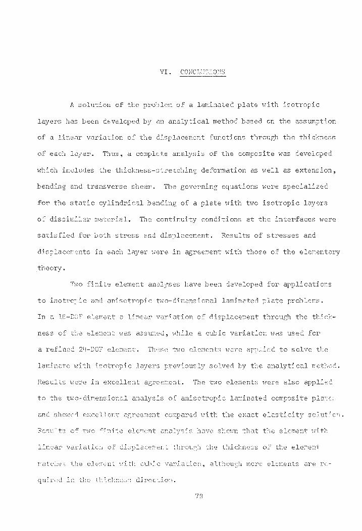
VI. CONCTUSIONS
A solution of the preblem of a laminated plate with isotropic
layers has been developed by an analytical method based on the assumption
of a linear variation of the displacemont functions through the thickness
of each layer. Thus, a complete analysis of the composite was developed
which includes the thickness-stretching deformation as well as extension,
bending and transverse shear. The governing equations were specialized
for the static cylindrical bending of a plate with two isotropic layers
of dissimilar material. The continuity conditions at the interfaces were
satisfied for both stress and displacement. Results of stresses and
displacements in each layer were in agreement with those of the elementary
Two finite element analyses have been developed for applications
u
4
to isotre;ic and anisotropic two-dimensional laminated plate problems.
In a 16-DOF element a linezir variation of displacement through the thick-
ness of the element was assumed, while a cubic variation was used for
a refined 2H-DOF element. These two elements were app.ied to solve the
laminate with isotropic layers previously solved by the analytical method.
reement. The two elements were also applicd
to the two-dimensional analysis of anisotropic laminated composite plate.
and showed excellen ment compared with the exact elasticity solution. ct 93)
63 5 o p
Results of two finite element analysis have shown that the element with
lincar variation of displecement throuph the thickness of the element
“ L matches the element with cubic variation, although more elcments are re-
A true three-dimensi onal
veloped for applications to nomhemogenecus anisotropic laminated plate
problems. A curved isoparametric element with cubic displacement ex-
at. tion of disp }4 pansion in the plate plane and linear varia acement thrceugh
the thickness of the element can be applied to solve arbitrary shape
boundary and severe normal warping problems. Results of the finite ele-
ment analysis for a 3-ply laminate were in good agreement with the exact
elasticity solution, even when only one element is used for each layer.

10.
il.
12.
BIBLIOGRAPHY Te
Calcote, Lee R., The Anaélvsis of Lamin Van Nostrand Reinhold
Pagano, N. J., "Exact Solutions of Composite Laminates in Cylindri-
cal Bonding" , Journal of Composite Vat a
1969, p. 398.
Whitney, J. M., "The Effect of Transverse Shear Deformation on the Bending of Laminated Plates", Journal of Cormosite Materials, Vol. 3, July, 1969, p. 534.
Pagano, N. J., "Exact Solutions for Rectangular Pidrect Tonal Ceom-
osites end Sandwich Plates", Journal of Comnosite Materials 5 5
Vol. 4, January, 1970, p. 270.
Pagano, N. J., "Influence of Shear Coupling in Cylindrical Bending al o } 1 of Anisotropic Laminates", Journal
fF Composite Materials, Vol.
4, July, 1970, p. 330.
Whitney, J. M., and Pagano, N. J., "Shear Deformation in Hetero- geneous Anisotropic Plates", Journal of Annlied Mechanics, Vol. uv 1370, Pp. LO31L.
Ergatoudic, J., Irons, B. M., and Zioenkiawier, 0. C., "Curved, Isoparametric, Quadrilateral Elenents for Finite cuomen’ Analysis", Int. J. Selids Structures, Vol. 4, 196 p. ?l.
Smith, C. B., "Some New Types of Orthotropiec Plate Orthotropie Mat ' 5 i 1953, p. 286,
Washizu, K., Variation Methocs in Flasticity ana Plasticity, Perga- eee en noe 2 A RE ANN RA RN Se MRR MT 3 wen,
n
mon Press, 1U68.
Reissner, E., an Types of Net
actions of ti
hing of Certain a
mM
2panair- ———
Dong, S. B., Pister, K. S., and Taylor, R. L., "On the Theory of haminated Anisotropic Shells and Plates", Journal of the Aero-
space Sciences, Ausust LEn2, p. 869.
hr T me - y Se f V7 tt aarti IZ LT. marie fiwnrta Whitney, J. ., and Leissa, 4. W., "Analysis of Heterorenecus Anise- 3 2] -34 ~ ff T, x ore Vtg 1 MA AI anita Of 5 tropie Pletes’, Jourrel of frplied Mechanics, June 1969, p. 261.
on
Ashton, J. F., ! Ppproxinate Poletti ons for Unsymmetrically Lamirated
Plates", Journal of Composite Miterials, Vol. 3, January, 1959.
pn ee ty a a A., Theory of Anisotropic Plates, translated from th Pusehe 1 by T. Cheren and edited by J. E. Ashton, Technomic Publishine “Co., 1°69.
Yang, P. C., Norris, C. H., and Stavsky, Y., "Elastic Wave Provarsa~ tion in Heterogeneous Plates", International Journal of Solids oO 3
and Structures, Vol. 2, 1966, p. 665.
Ashton, J. B., Halpin, J. C., Petit, P.
Materials: Analysis, Technomic Publi
H., Primer on £0 mposite
is
Abel, J. F., and Popov, E. P., "Static and Dynamic Finite Element Analysis of Sandwich Structures", Pr ines IT Conference on Matrix Metheds in “tructural Machanics , Wright-Patterson 2.93, Ohio, 1968.
QO OQ D oO fu
hag 3
Zienkiewicz, 0. C., and Cheung, Y. K., The Finite Element Method in Structural and Continuum Mechenics, McGraw-Hill rublisning Com- pany, Limited, London, 1967.
The Finite Element Method in Engineering Scierce - ;
4
Cloush, R. W., "Comparison of Three Dimensional Finite Elements",
Proceedings of ‘ of Finite Clement
Methods in Civil &. Sey ACCT, “eno University,
Nashvilie, Tenn. Mov. Luce.
Zienkiewiez, O. C., Ircns, B. M., Ersatoucis, J., Ahmad, 2 and Scott, FP. C., "“Iso-parasetric and Associated Flement Families
sion lysis", Chapter 13, in Finite on ~~? . - - 4 for Two- and “Three-DMmensional Anaiys. 7 Element Methods in Stress Ana
Pe ee Te as Dane Teer city ny at y 2 Techn. University oF Nozvay, Tapir Press, Morvay, Trondheim, 1067.
Pryor, C. W., Jr., "Finite Element Analysis of Laminated Aniso- tropic Plates", Ph.D. dissertation, 1970, Virginia Polytec nic Institute and State University. a
Tsai, S. W., Mechanics of Comnosite Materials, Wright-Patterson 4™,
Ohio, 19C6.
Weaver, J. W., "Finite Elenent 5
Ph.D. dissertation, 1070, Virginia Polytechnic Institute anc State University.
“+e Wy ft - 4 ren OTT en Sy pe a Ay aT mvt Hatt, T. Fink erent Andlvsis Using GConaral Iscrarametrt ;
I
b 2 1 .¢ ~ * * « . ro a
aya" “HSCE thesis, LOVL, Virginia Folytechnic Instivute j

82
26. Ahmad, S., Irons, B. M., and Zienkiewiez, 0. C., "Analysis of Thick and Thin Shell Structures by Curved Finite Elements ," International Journal for Numericel Method in Encineerins, Vol. 2, 1970, p. HIS
27. Frederick, D., and Changs, T. S., Continuum Mechenics, Allyn end Bacon, Inc., Boston, 1965.

APPEUDIN A re
The elements of selected matrices used in Chapter IV are given
as fFolilovws:
Cubic-Cubic Shape Functions Ny
Ny = 1/32(1-8) (1-2) [9Ce7457)-10] Ny = 9/92(1+3E) (145) (1-87)
No = 9/32(1-3E) (1-0) (1-57) Ng = 1/32(1+e) (+0) L9(E7+57)-107
Ng = 9/32(1+3E)(1-7) (1-6) Ng = 9/92(1-E) (1-35) (1-27)
Ny = 1/92(140)(1-2)[9 (£7407 )-10] Nig = 9/32(1-£)(143¢) (1-27)
Ns = 1/32(1-E) (14) 9 (E+ -10] Nz. = 9/32(1+E) (1-30) (1-2)
Ng = 9/32(1-3E)(1+5)(1-E*) Nyo = 9/32(14E) (1435) (1-07)
Nior Ne sr
Cit = 1/32(1-0)£9(28-36°-¢° +10] Coy = 1/32(1-E 09 (20-307-E* +10]
Cro = 9/32(1-0)(967-26-3) Cop = 9/32(1-38)(E7-1)
Cyg = 9/22(1-5)(9-987-28) Coq = 9/32(143E) (E71)
Cry = 1/32(1-n)£9(2e4387 +e°)-10] Con = 1/32(140)19( 20-907 = 8" 4107
Cy5 = 1/82¢1+5)L9( 28-38 ser )e10] Co5 = 1/32(1-E)[9( 204907 +£°)-107
Cig = 9/221) (e223) Cog = 9/32(1-36) (1-87)
Cy = 9/92(1+0)(9-92"-28) Co7 = 9/32(1+3E)(1-£*)
Cig = 1/32Ciec)fo(2e+3e*+e*)-107 Cog = 1/3212) C2 (2088e 4e*)-10]
Cig = 9 92(1-3¢) (07-1) Cog = 9/32(1-£)(65°~25-9)
Cyiig = 9/32(1455) (5° -1) Co ap = 9/9218) (3-95-20)
Cy = 0/32(1-92) (4-67) Cod = 9/32(1+ “\(or* 07-9)
Cy oqo = 9/32(148E) (1-27) Co gp = 9/82(1+5)(3-90°=22)
83

gu
All elements of Bes aro zero, except the following:
Bay = Ns = 1 EF oo6y4-FyoCoa Fs 5 = 1, 25 02-12, i = 2j-l.
dx = J]
-~ ONs Ll _ - 4 = = Bos 1 = b41%55 F510 443 5 1, 2, ...12, i = 25
gZ EJ]
Ba; = Bia) P=e2,h, ...24, 7 =i-t1
Bas = Boy 1=i1, 3, 23, 7 =127+1

APPDEEDIX B
be. The elements of selected matvices in Chapter V are given as
follows:
Cubic-Cubic-Linear Shape Functions N;
Nig
>
st
1
1/64(1-E)(1-n) (Aer) £9 (Een )-107
9 /6u(1-3E)(1-n) (1-2) (1-£°)
9 /64(1+3E)(1-n)(1-¢) (1-87)
L/64(14E)(1-n) (1-2) [9 (En? )-107
1/64(1-E)(1-n) (14 c) £9(6°#n7)-10]
9/64 (1-32 )(1-n) (ite) (1-8°)
9/64(148)(1-n) (145) (1-E")
1/64 (14E)C1-n) (140 £9 (E74n7)-10]
9/68(1-£)(1+3n) (1-2) (1-n*)
9/6uC1-E)(148n) (1-2) (1-n7)
9/6N(1FE)C -3n) (1-5) (i-n*)
9/6u(14E)(1+3n) (1-2) (1-n*)
9/6u(1-£)(1-3n) (1¥5)(1-n*)
9/6u(1-£)(143n) (14) en’)
9/16(1+E)(1-an) (145) (=n)
9/16 (1+E)(143n) (140) =n”)
1/64 (1-E)(14n) (1-0) 19 (E4n*)-10)
9/64 (1-88) (Ltn) (1-2) 1-5") >
9/64(1435) Clin) (1-7) C1-5°)
nh 2 L/64C14E) Clean dC1-7)£9C5 "+n )-10]

Nol
Noo =
23 7
86
2 2 L/GUCL-E) Clty) (asc) £908 ¢n )-10]
9 /6u(1-3£) (len) (iet) (1-27)
9/64 (143£).14en) (14) (1-27)
L/GUCLEE) (len) (14x )£9CE2 47 )-107
1/64(1-n) (1-2) L10+9(2E-3%=n7) I
9/64(1L-n) (1-0) (98°~ 28-3)
9/64(1-n) (1-0) (3-2£-9£")
1/64(1-n) (1-0) L9( 88749428 )-103
1/64u(1-n) (140) £1049 (28-387 -n*) J
9/64(1-n) (140) (96°-22-3)
9 /6u(1=n) (147) (3-28-9687)
1/64 (Lan) (Ler) £9( 38747422) -107
9/6"(1-8n) (1-2) (n*-2) a oN\e yf 2
= 9/64(14+2q) C12) (n°-1)
= 9/64(1-3n) (1-2) (1-n*)
= 9 /6uC145n) (1-2) (1-n*)
= 9/64(1-3n) (+E) (n=)
= 9/64(148n) (142) (n*-1)
= 9/6U(1-34) (140) (1-n*)
= 9/64(1+0n) (140) (1-n*)
= 1/64 (1tq) (1-7) £10400 28-35 %-n7) 7
= 9/64(14) (1-0) (06% =28-3)
= 9/64(1+n) (1-7) 03-28-95 cy
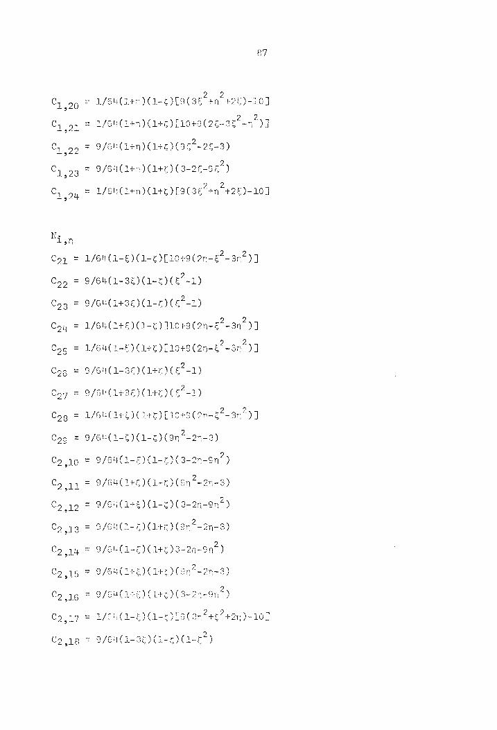
= 1/64(14n) (1-2) [9(36 +n +26)-10]
= 1/64(14n) (142) £1049 (26-38)
= 9/64(1+n) (140) (98°-28-3)
= 9/64(1in) (140) (3-2E-9E*)
= L/6uCL4n) (14z) £90367 426)-107
= 1/6(1-£)(1-t)[10+9(2n-£°-3n7) J
9 /64(1-35)(1-0)(E°-1)
g/6U(143E)(1-0)(E7-1)
1/64(1+E) (1-0) ]10+9(2n-&7-3n*) J
1/64(1-E)(1+0)[1049 (2n-£°-3n*) I
9/6U( 1-38) (140) (E7-1)
9/64(143E)(140)(6°-1)
/6uC145) (140) £10+9(2n-£7-3n")]
9/6u(1-£) (1-2) (9n*-2n-3)
= 9/64(1-E) (1-2) (3-2n-9n7)
= 9/64(1+5) (1-0) (9n*-2n-3)
= 9/61 (1+E) (1-2) (3-2n-9n*)
= 9/6N(1-£)(1+e)(9n7-2n-3)
= 9/64(1-£)(1+5)3-2n-9n*)
= 9/64(1+5)(1+ze)(9n*-2n-2)
= 0 /6uC1l+E) (ltr) (3-2n-9n7)
2 = U/CR(L-2)Cl-r) £9 C an? +7 4+2n)-16)
, 2 O/6NC1-38) (1-7) (1-27) a
‘

Cy yg = 9/6N(L#3E)(1-5)(-E)
Co 20 = L/6UC14E) (1-2) L930 +8420 )- 10]
Cy oy = L/64(1-E) (140 )E9(8n +E 421)~10]
Co no = 9/64(1-36)(140)(1-E°)
Cy og = 9/GU(A+3E) (14) (1-8)
Co oy = 1/64C14E) Cite) £9( an 40% 42n)-10]
C31 = 1/64(1-£) (1-n)[10~9(8°4n7)]
Cyp = 9/64(1-36)(1-n)(E°=1)
Cag = 9/64(1496)(1-n) (67-2)
Coy = 1/64 (1+5)(1-n)£10-9( 6 #n*)]
C35 = 1/64(1-E)(1-n)[9(27#n*)-10]
C3g = 9/64(1-35)(1-n) (1-87)
Cg7 = 9/64(1435)(1-n) (1-87)
3 = L/64C1+) (1-n) £9(6%4n*)-10]
C3g = 9/64(1-E)(2-2n) (u*-1)
C3,10 = 9 /64(1-£) (1491) (n*-1)
C3,11 = 9/64(1+E)(1-3n)(n*-1)
C3,12 = 9/68(1+8)(1+3n) (n*-1)
C3,13 = 9/64(1-£)C1-3n) (1-7)
C3,14 = 9 /64(1-£)(1+3n)(1-n")
C315 ° 9/64(14E)(1-3n) C1-n*)
Cy ig = 9/6uC1+E) (1430) (1-7)
C3.a7 = 1/G4(1-8) Clty £10-9€ een) T

C3 jin =
C319 =
C3,20 =
C3 21
C3,22 =
C3,23 =
C3 04 =
9/64( 1-36) (tn) (67-1)
9/64(143E) (len) (e°-1)
1/64(140) (tn) 0 10-9(E +n) ]
1/64(1-E) (+n) £9(6°4n7)-10]
9 /64(1-35) (L#n) (1-87)
9/64(1+32)(14n)(1-E°)
1/64(14E)(14n) £9(E74n*)-10]
All elements of Bis are zero, except the following:
Buy = oN = [JI(1,k) C(k,j)]; k = 1,2,3; G7 = 1, 2, ... 24, i
3 x
By, = SG = [oT(2,k) C(k,j)4; k = 1,2,35 J = 1, 2, ... 28, i oy
On. tos : Ba, = Vj = [UI(3,k) ©” (3)]3 k = 1,2,33; j = 1, 2, ... 24, i
dz
Buy = Bay> 1 = 2,5, 8, ... 71, j = i-l
Bus = Boss 1 =1,4, 7, ... 70, 1 = jt]
Boy = Bays 2 = 3, 6, 3, ... 72, } = 1-2
Bes = Bas3 P=zel,4, 7, ... 70, J = 142
Bez = Boys 2 = 9; 6, 9, . 725 J = 1-2
Bey = Ba45 1 = 2, 5, 8, 71, 3 = i-l
where
JI€1,1) = [802,2)008,3)-3(2,93003,2) J/1d1
JIC1,2) = £ICL 30038 ,2)-J01 20005 3) 7/101
tt 35-2.
35-1
33

JI(L,3) = [001 ,2)002 39-301 S002 2) T/L
JEC2,1) = [002,3)903,1)-002,19903,3) 2/21
JI(2,2) = [5€1,1)003,3)-0(1,3)903,1) V/1d1
JI(2,3) = [3(1,3)0(2,1)-0(1,1)0(2,3) ]/1d1
JI(3,1) = [0(2,1)59063,2)-3(2,2)003,1) 0/101
JI(3,2) = £9(1,2)9038,1)-3(1,1)5(3,2)]/i01
JI(3,3) = [3C€1,1)5(2,2)-3(1,2)7(2,1)J/1d1
Cubic-Linear Shape Functions N, 1
Ny = 1/32(1-6) (1-n) (967-1) Ns = 1/32(1-E) (14) (98-1)
No = 9/82(1-36)(1-n)(1-5°) Ng = 9/32(1-36)(1#n)(1-£7)
Ng = 9/32(1+36)(1-n)(1-8°) Ny = 9/32(1+36) (itm) (1-5°)
Ny = 1/32(1+6)(1-n) (987-1) Ng = 1/32(1+2)(14n)(¢e*-1)
Nye Neon
Cyz = 1/32€1-n)[1+32(2-38)] Coz = 1/32(1-E){1 L-SE")
Cio = 9/3: 2(L-n)(95°-28-3 Cop = 9/32(1-38)(6°-1)
Cyg = 9/32(1-n)(3-28- 36°) Cog = 9/32(143E)(E°-1)
Cay = 1/32(1-n) £96(2+38)-1) Coy = 1/32(14E)(1-96")
Crp = 1/32(1in)[1+96(2-26)] Cog = 1/32(1-E) (9% 57-1)
Cig = 9/32(1#n) (S6°=2-3) Cog = 9/32(1-3E)(1-£°)
C,, = 9/92(14n)(9-28-96") Coq = 9/22(1438)(1-8°) 2
ut = 1/32C1tn)09£(2+32)-1) Ca L/S2C142) CIE -1)

16
APPENDIX C
-DO \ Po Procran L
OL

92 T+¥9N
= WIEN
OF O
= N
QO =
$TGN
(COTZ* AST
TV) SLIM
37LIL
Vivo
(MG1539N)} TSWAS
113
SAN3W39VIdSIO
L1ND INldad
ONY 2LVINDW
3 44TiS VW
XTYL¥w
SSANASATLS
Wadd
3 IWNDS0G
TW)
T =
JOVd!I TS
O3H
(GOCS=GN3*OCOT*SOXSIT)
Gvau
0s
WY¥HOGdd
FO NOTLYNIWHSL
YO W379Cdd
MBN
AD LYVIS
YWOAS WOISHD
D 9
=1$14
GS =
Qa!
(N*£7*O000G4999)
2 ATTA
JNESIG
(arr*a*§oo0s*o99)
T 3tld
3NTaaad
ZONSGNS ONS OFT
SIENNA SCOOT
IG SIZE foot
/ NIGS
/ NOWWOD
SANS INSMETS IdALWS LAWN
® TOWN
SA NWON
£65 9005 XI
¢ *(94*8)9*fOCS)S9*
(905)SV¥ T
S(OZSTIZNS LOSSTIKENS COZST
IZ FCO2STIX*EGZST)3IG09
/ WALVG
/ NOWWOD
ANIM I9NVdTS COZPOSHS
LST Vaud
7 OVIH
/ NOWWOD
3995
MSOALNY
(7-049-V)
Se WIet
LID dw!
SiNSWITS
HV INONVLOSH
YyOd WVHODdd
(SOON
HOVE
LY 2)4d0C-9T
wad OD
¥ €
é T
X mew
n-+ 3
Q-----)----~0--~---0 (
2 '
i |
2 j
| Z
2 Qarn nen
Qe nnn O-----0
3 8
L 9
S 2
SSLTSOGWOD
GSILVNIWY
TYNOISNSGWEO-2
40 SISAVVNY
INaSwW379 3LINISA
9

93
(7-949-V)
es Wau
ft
JL ESIT
NS EON
aV49 a4
Gudd a NOTAV
EN Gen Pld
LAD
ahiT
tm
= ot
by cD EWC
Tae
4d OX
ETE PALEY
TE OMT
fe RDN
Bey
mai
NAVA
LEAN Lvs
is TA
ENTSMd
Gey
GLy mutes

Qu
‘pel S(3cALWAT)3
e
1!
wont
be DN,
mee
) }
mn
by
fl cALA
ate %
~~
“Ch
LP)AL
Re ‘ ANK
AN (08 0
mn!

95
N €Q8T0
28ST
VE 2h)
Saye obesad
(PSV)
((2)7
- OF)
2) Se¥5
CRS]
(7%
= €9)%)
(fi) yx1l=
yx I
Wis TAN
(C8T-NPXT HOGS}
Co (18TH8)XI
(14N)
#*T=] 4
SGT EGLT EET
(K-#)
§
"i
2 geet
WI LY ed peed
we (8 tT
2 Fs
eT beet
(7
ee
MN
nm ova
ee rol
EYPFV EMR
MS CHF
2b
ES
wE

96
~
) SV Foy AEs
LaDSCLANDX
TD EN (EOC e
che i
wal.
shen?
an NH
f¥ OT
Ly X
seeteecs é Ce
Fee FXT-€]
>
eet
ae
SETS
OT ESRT On
Tea ope
age
8 ord
te, >
Met
i
t pond tt

97
(7-25
SAIOV
NI Xdsives
4900]
PVEnoyva
Le (9 PEELS
T BANS]
Thii
3
CES TASTOSEV
ITD ZHET EXE
ETF
iS bem
p=
W4t
fee Std AL
LWEQd
VW é
om rem
{cc
tae
fifcth*:
be

98
*¢ ty
we ta
34°
LE Te
(Peupxs
STHi
SLOdAAY
a
PTS
ih OF
€ |
XTuive
ssi
MTC ANG EMC]
OC} TE
ONIN)
S3nT
bea
Es
S THE
SITL9
any
T+ wf vi
4:
41
(4 A)¥
¥T

99
me!
wd
a
=
frye
Po
COTS Tar
eet
ht=al*$ i
fT )Sy)
(itsyo
+ Off)
4 é
Lea OE
UNE oye
8 ir
4 ays
Set
FT
Kt
oO
amt
~ ~~
iN ~
a
-
rm
peost
CPSiyu sn
O84tye +
Of:
"LTT 29
x
(N
wae

100
4
FOVIT
SE LG!
"Loe
vn,
a .,
ne
me i
Bw o
il a
few
<4
Vo LNFONG
SPT
LR
SANT
LNOOD
C1!
sHHedS +
CR ATIpY
= Cres

101
riiet & <
CWA
aw fhe
{ a
\
é
PucT
TEE
Ee
L¥RL
Sig OXS
fcypfe=
MeL €T=re
(ane
®yted
¥
ae t
dQ LALHS
Gn
342 (
3 miié yn
¥ )
jay
7 ty
5
w SSSN4ITLiS
OTL
(NSE
7S
4 YVHEE
TAX so.
(cf 1) XI
FWA §
(dNWON
Say
Peat
oe &
JL G8
yw é =f*(r*tiv))
HEOPM ONY
PH Ob Ey
ah
eay
(yes
wb -
CTTe
ete
a
se
> £4
2
t
HT — T=]
[St
ATT
) At
LS)
te
T=
Ve

102
*{
(& ye
2 *
(257
(7Ennwet
Peat
yt:
sly
LOVIsEL
pov
TEAK
+ Tenn
—
sew ue
wrt goof ONY
retired ON)
leading’
AN
eda
i
mM sre
a Sty aaa
oe, ‘ wo
t
che (ee we CAR K
~ETANX
me TANK
(Ve (FL)
(75:
eet Wow gh hadnt
poe
pw eh

103
(Ta
de:
CTPA
T) fd
ee.
SIG
fe
Beit acai’
(7-4 5-4)
4.) SOREINT
SJOACS OLS
“HAF
ee od
Fad F
ay ot
en
“
“LS
seed
oy

104
vt é
CEUs Cayo
fe Tet
pve
ay ot
F
©
i
:
ry
2
med
I
see cat Oe
on peed od pend pe
-
ad
- a
. ' et ee
f
(S FE
VHS CW
ach TILES (aa
(ST bys
+
re
had
on NI
we
ut
on
- pow he
- ne Phen ce "1
gett art, oO . i? rey og
pepe ei
Pe oh Fr Fh Rh FP hh - wi
em Es
FE ee a oes wn ke
(
“
red oom St wo
we
i a atti
ue ogy ”
Le" ZAEC
PEA EGP THEOL
Eb)
4 4
Cotes dont?
: ( { (
wok
con
an
- m
Om a
~ oF 2, pend dere
-_ he Ph hh fF hh Om ® we
fee - oe
4
fh
€
abe “
vr car, ty rey
Act

105
ey
vel
Cs
ped eed
il foot
ner pw
d 1
~ sat
we ee ae ae
it _
if pr wie gee peed
a4 bad
to (%
eo 2
pas Oo}:
Lys +
€5
(ote LE
CtRaS
ve G¢Leiyit
+ (£49
S4°SFECe TEL
& UE
TOGA SC
OPTEE DH
# CST
AZ DE
tt FH cata, eed tej
aa
re
ery,
Les rf
-
. .
et
ee
+ fig ®
co OQ J
ry
are)
JO t
Cx
o
(NOS
(PhS T&F
ESTE aT oe
E*9T)
ff 37a
Pd ALYY LYRA
EINE TAR
ON fINWON
EGE
tte
ae (cep saee
*EDZET PENNE
CSC STINE
CST ITEC
EST KE
CCSST IAG
PY VEE
EST EOLYSSCOTES
INE MOT
oe
oO
ue

107
“TES 1: oa j
NIALL
(eff ey 4
(fe
XTHL Ye fn
fyy
3*hOT)e ‘yy
SS.
Ad
(rs
y
god
“at as
108
oy
pe
i” +!
i
ied
2% mes?
on
5. ay ‘eowal
a
/ ( may é
(T4N)¥
/ SFE
OL OF
| Fase
AN ae
| 6 4 See 2
de TOT
GL OS
€ 6
TORT MTUND
- Ce they
OOo) eCMaT
STEP ECHNE
WET SCP A
TW)
OOCL aT)
Geay ve
it (TTs
yds) =
XT 222
GL OF
€ WIECNW
"Att YTUN)
4I Santa
dO yoOT: a
hone
s
peri
(hn SKN)
Y=
POM
ay eo
fat
Toe To Nwe
€49OT PE
EP
Litt ldaal
C2 AES
UACASy
2 4+.)
W4HbsASN
SHE
AATGS
J Rw FES

1093
fray ®
(4 de
(T)ex (fp
yy -
HG
GN
hb
40
PaaS TES
ES NV BONSNG
%
{ oo] of
(RN *&T=Ye
Os) Je
ORS PEPER EEN
S THT!
CP eT
eu )) CMP
eT) alex
Ct -
(Ttea te)
of
Yown 64992
( 0}
(xf Ndbved
- Cf é
A i bai)
4 ef
V4) e-tl)s=
(1)8 *t) ) +
seed
BY
oat
=
~ #
“
rae
fm
fy
met
iy. =¢¢
(re ryy
m
ms
wi Sad

110
ey awe at
rod pend
TEETIESCLPOTS fO9LINS
ESTES)
POUT POTS
ACE Teal
ECOL SoS
fyr LEA TERN
(HOT Put
(ce F007)
ORT BOA Ee ia
OT
EAN
f(eSeyaeene
K4(025T)3009 /
whava / /
we J2O4
ENT
aad
LEP Tdht!

111
i a,
Yl ds
yew
Ly ae
4
e PekCEVOES #
Pe e03
Cetsb hy
((E)8 /CEVIESYNYLVODS
=U
ee
if it’
ot
SU° Ge
vef5e%
oh €
Ce
Mt
vk
mae Smee “ =
NVLY
~ (fT
DU-¥
JOV¥S
dix
eleeyOTS-€i):
H#((P)OTIS+OT)
SAgbksS WWalowl
YG ub
(Fane
OP STIL
+ CPST!
OEST
(To -
d)&E
i
(ta
v C(T-XUEN)
& IR) HT
+ ON
T +
IN/ ET
) (Il
- Pee
+
|
foo
fh GO
SOLS
S). al
t

112
TL O2
FR cet me
(kts
“e ~+ "(S47 K1
"CNY
OT Z/CL
Lt cern
(LZ°T=ES C108!
C2STHTDF CDOT ag
sila
+ LSa
PISALS
COTS
M447
LS
FETs
( iG
*T=r*er*lys))
JD 8 ANGST
6-96
eh Of
692 (T
tT +
S)SHFN
(edu zF
S) 4H
2
GG OF
5° {
(OCO74L
wh G2
(3b *%
17
CE5)959TS -
(FPOTS Seve
Ts
“hs
(Y}OTS
4+ 07°
(2)91S
4
C i * e
£
H
(YISG
= 8D
‘eyxX] =
YW
: é £ ei
ANN TIED
Sy} F)
JLT
PTLTL
PEGS
int
me
* 3417)
ai
= (230)
AON TLS
VW CR UA aa
oT OL Tl
ay OL
8 &
Capo f
POL
OF
(FOTN
oF
ay
ot '
4 tes Ady i
wd

113
STONY
HS f KHACOD LS ANG
“st on
Sand >
> WS
Oo wn
~“ tm,
5
7
L
~*~
Fated
5
>
4 ts
m™ OM ~
ad ON TO ~O™N ——, ~
Bd 1.
E
COTSZTILSELIOIS FEST
IANS COTE
CHOP
EIT SSTES FCOTES
TES SUCTS
xT ya CaTes
CANFANE
RO TE SAALAS
EVAR
“COSSTVAP
ECC ZOT IRN
EEL Cot
(ero
Lg
("Sot
(4 foTaée
(+
SMASH
VRHO Layee se: SOO
EX OF Teste
oer’
»
”
ne
cre
§
ye “}
*
t¢
in
SS IMLS
HTH YE
FOSS
a aL. wie!

114
AANTENOD
os
SPNT
ENO o
(ro TL
Ct
Ul
(Pea atafdyoa
+ (Ff
TDL 9Tf
Ts
2.
i
u
aoe =
(red)
4%
4 =
iH
SUC
PHOT
ace Ho
Y-
(TIG/OP
Sa (hd
Cu mm
~~
pond
see Cy
3
~ ond
i a
ae
v aa
Cad ®
‘ EN
i iH
— «a,
gore gooeed
mont get PE Vt Pee YY”
VES
(LY) 4«27
CL }GX Keo
tH
c
tt

APPENDIX D
24~DOF Program Listing
115

116
e
SONw 4
rie
CSPZNE
ES Gxt
INET
fS9ovd 1 &€.
@NIweF 1 PUNGE
CHF LATE
So Gol
palloe
C205
)7 ©
‘L444 FL
ST7
wv dtide
ow ew
m
Y Je-+----tj+----+-:
SNikw
EC
LEXI
* €40:
(: Is
(tray
d
At } x e
S
ed
-—-—-+
=
f Viz
93
SISA
VWNY
ae cee ee
ee ee ee
woe
LW
Ly
Ti
is 1
ADTs
et hh ad Sat RG Sa t C3
117
TN
a fik
OW ay
aN
UE
bASR
SS aN ee
Uh
Sl TititdGad
Wits
lve Cae
GAY CdNS
AN EME
A EUR WON
fT
IN fo
Ain
§ CET
SD xIC
9) 300" ae
(OGTISBe
CL CTS EEE
Wie (o
4)
Col3)24OE005)K%
/ vk
ON Fis
CE Tava
® (OL PGI
S LS rye
/ ‘
FO
(2-2 fH-V)
Bad
Ps LIST
tawd SOLiSledaa.
WATCOMG
SAL 45
NDTL
(VdSTO-7HE
ORE
T fh eS LO-KHL EX YY
(MTSENE TPZ
8 Oa
Te
a
118
ot mere
*
4
ZC +e yz
XG +#(0T-1)X
id (tT
“eat
© =
€F)S000Tr
¢2 that
oom,
pd
I
at sneer
the
ale te foord
ft i
> oe)
AHN
ET ENOD
XZ/ ECT)
Z-ONI
ZF =
Ze KEA
COV XO
dR] =
XG
-- oé
Se
(INEZ EEN
XN EON
EE ZEON
K EER)
aS
Ce. €fiSE4)
ail de
ThLIL VWs
VLVO
GNTUd
PYGON
uf he
wee
(9 *l=LSisdaAiatiysa)
43dal
ee OL
Go
(S*T=f! (4dALat fia) fad
(ZTGc FASE)
(iTac*LSid)-
aM *
Ly AON
© LAN OIM
f ad way
LS tt
} or
bd

119
ROTELOTEE ST
CCL Z
— C107 08)
COLX
— C41 St
J <i
on pom Téw
KTS 1
O98 Ce TAT-NJXI
CTENDXI +
CIST-N)XT =
CEENDXT 251
EL‘S=] 261
uC e+
CISTANIXE =
efter Tal
OSTHELOTSL ST
i. i
femet —
fomee NE tone
, ”
ae Sees!
4 LS
ped
ey ue
sree pers
on, wor wT
mere 2
wt
+ cay
iJ ce
xt
pod
ve mle
f4%
2e {far
tt rE
(1x9
(STST=IS
CLP AXIS
oe
pe
tof
wont
Sad
eo
wd onal
to
pwd weil
No (&
Loe
Epe.
oF Mi
:
EXD ZNSE
CAPXGE ODE EOD
KE Cd soe
DE Sa OGL
oO PEESE
DT) i
+ anid
= >
(Fics
kLSbPT) Gliese
=TEtL
WW
[6 GL
OO (AG
*44% FIR)
Sl VAIN=y
26 06
7
feet
or
“Add
o ae
~
co
be a
us
wnel ee
‘mm, pot
te :
“ZLPINH
# exe &
120
CLEXG f4L0N
IX
SNOTSTAIC
&
t és
sGAL
C(° STIs
GT) -
CUO
= ¥ oa
eo, &
an
(SS aN%01
Lue
fei fC
T9HY
ECSHE fx
& oe
Me
OX {Gyeerte
* eae:
/GTEST 8SWH
1&6
yéeorer
{GE eens
40 (SLVh
Vout
aiete
f*ck
Is
Ta
‘AN
NOTLS AO
}
ih
TDS
iNers
«*
}
LNIud.
®XoT EOE
xs
43
NI Wad
wad fee
hl Reh
COTENYXI-ACT SS
3 Gg
fo:
4x
fG
py
(4a
é +
ALT
e- OF
Ms
“hy 1é}
*u1) vi)
t)
fs
wie
anD
dp} tl

121
dt SON
*MeET & bya
AN eqs a
fin
(2*2)ytrc&
(ete
‘ bie “pba
1&
rue
*(GATISSS ECTS YS
NT qeas Sd
49H4 iS]
44 an
(Z-134
WLLL
40 NOLLY
Od
ret Samet bend
XESLVew
SSINAATLS
SLES
CW
aoVvdI SH
FEST TAGHOT
(Z-u4H-V)
GELS ANN Tea
SSaqdis
ANV Ud
é
2
S1ZT*xe a 3805}
fas
dead TG
d
wt N
ot
ol
blake!
Lae Fee
£ ae
iM Sue ON ey o
122
“ (i
*NDKE SCONES
Ty *a0%
©
S42
ST
“Lt
€3
“VaNS t
SoMa
SGaNsdTiS
WLU
#0 HOOT.
STHL
Shodan
Ste
Jk
PuUaWAN
At X LUE
same
fr o%
iNT 48
SHOU
NE XTeiv¥aw
Ss: Ws
TINie 444
HHENNAW
SSH9O
TE 4b
S35 lekLve
dee Mulag?
tifkl

123
bet ul
CSP
GUSTE EC GEG
is
e; oe
‘si e.
i +
GNRIN®
THN
ooe
Ua
SSUGN
LY S50 404
GSHiv (LR
SNOT
MT LNG!
+
(114 He)S
+ CFPSTT
VG “tre *tiyy
| GULLS
Cr EMD
ESOT OPER
ESN ET
ON Fe OZEEST PE)
FLIUN
eoTe
ste et
(fF f-Mel)
41
Tf 228.02
(ff)
4l
= 1
Z rt oaF
» 4}
ge Ske
ES
7
ond
i
Sei ~-
T+
TIT - V+
7 -
(PN)
rt Hout ae at tte
ste a
I
- &
et:
a
me oss
at
feet oe
Me
tl
MS
x
at a Pen
2 e
3
me po
’ -
Free geen pet
ifs dl oon
oo
~
ms
(i =
HV
(ET EN
on
(NIAELS
12 VG
£
y
GS Cin
OS Ce
CAN PKTSONVS
Gause
FLV
DG SGNES
o-GG"
SLIt
VO)AT
erred Way ERS
oy TN
fae
4

124
(GN
f Too
©
HJGTS M4MOT
dQ LSTHS
IN’ WSIG
Nu Sworawas
MPEP OMT
* 1 =F
SCGN
STEHT Ser
ebay)
+t -
[
wr tb
Do €
€an~w * bee
pert
d\n
é—=
ww)
ee,
wf mr
t i AEN
YE
Ve*T=w Ze
a6
CGS. = (¢)8
(x)
Hh
yS
3
ee, i
i
-_
G
wh a
Cab tak,
(WX
Sh
N )
Al
fom
Ce dR
hae iL
UO

125
“(ZT
S 25% Cee
GNS4ANFEMGT
f EUR
foc ctpsae
at Tb
WON
© TaN Of
a NIN
EOC
STISVS£
CO
Te DH
aL vw
rol ret
LL ened Me
“wy I oS
wheat KR
Room
pe fe “) too
ag
ite
Hix
€TCANKee TA
1G
ype pe
463
I1i/e
tla/22nued LAME
. 74
wee
wef
4T “
a
a
(24d. tra*(é
§Z rae
Ce FEVON
(et Beat ected
ul wenaeea
dacd*¢?
fl clixié (
ayent tee
)x ae
| GAZ*C:
S434
*X¥1laeive SSanNsdld
LRG
SG450%
feys=
HLGIN
J HTM
Oy 4 PVRSH
ont eee
3 ae 8, aan <a i y
vw J)
vile
ae |
126
i
PEST Se
OF
ER ZEEE
CdNf SNE
MELE EVA Wf
Top wig)
IGUIT AC
TES A
ELLSYK fo
wives yk
§ ag
Ne WAN
© CSETIS
FEO TISWE ECS)
ENS
S418 veh 40
INT< x fC
Fach
=
(
AHL® CO CANKA
EC TANK
FE
t nnd
ee Sr
Zep
ye
Vafiabe (ECONKXe 2LANX
= “Doe
cr gee £2
90G
LOVI/A
LEC CCN
ee
eX a
: Ny
BAY
eFINX
+ Telit
bx (cen
SINX - « 3°
Lp
(Te!
a
! “nate

127
a,
io 4 -
worl
»
Ce
!
i om
St geen
~*~ &
eotid= (6°T)9
Oe
Te ts
Yer on
(WR
Re
cue @ TV EA
*
Kk
t
beisr ita
Peale vy
YW 4e- (
ou*
T+
t
(CL) eh2-00°T)
(1 -
Fhe
+ |
=
se!
PF PLCK
eS
etre ax
CP PTS Ke Latte
cS Led
x
“i .
ae f
i}
a S
x WS.
ka he
ae
or
rz 6B
eet eel
“meet geet Tags
&
ore CTDWA
Ze S6-E
ee (PPT
SKR.
it
wm,
reed
»
per,
eet
XK,
AVWUOSSNGUML
*ONOGD
(EXZTIZXe(ZTKEID =
(exer 2X
xldLve *aCLD
EeTbd (Py
As Cle
(tT -
Ibs
128
COL Wa7e5 0°51
(LO*L2~-CT
18412. (CLVEZF
= Gwe
(l20°22-(1)
¢42
(FP ISKa
UGS aes
pel CT)Visse
DG Te-Cd*
el ]
1
ces
l TPES AK»
“su (PP
LSX:
an A
{ dy
“ ?
} 4
CEIGACT PL:
PFLAGACTS cdrs
PLIC/EEST
ILS
gee a
an ow
satel]
220d?
T-dax(L) idx
pu
wl CPP
TS xt oe
(2'é
(cf
Cot
Te
COP VTS KA LG
(5
PEP eT
ST PA
CCR
YES XE
oo
AE LZR
ope (CAPT
SA-
(214%
}
+ i ! fi
~~ - & eed
u
poss yernd
eo

129
at
{ oe
‘wa =e
}
Sit ite, >»
C42"
=f * Ce
ZS T=aLS
EPFL Sd)
(PSX eGaaGePLIGe
(RA
+ CTH
dS =
CTE ANS
oT
Sbte dt
oy 4
é
PP eS/ ETS
2 axe METRY
a
PO"ZE/
ETE ZG be
S20 1FG
meet Vey
aet of2)1F
9 S
"EE/CCVEE
Ie EE ATIF

130
Rob Gh
ee fe
Fo
CHA HN
=F ( We
leer etyyy)
€
i
oy a
my
rel
fi woe Bevin
es a: bevernt
pow
«, we
ba
TS om Le
MOUTH bal
NAHL
GNV
FSaF
TE An
SNE
ZN
fON fan Ord
fats
GN OCR SLE OES
SETI
(Z-U fH-v)}
COPLVV8s
SAGANY Le
TS ad
fa yyes
KaL SAND
1
ent
we
pond
y

131
<f
»
Po bend
fa Lil
of t -~
kwon boven
Gs
dard
fran! ty
Ge ag
fa 4¥
de: 4) YOOTO
GNZ SHa
SO SNE
SINGad
IT TEST NAGNDINA
}*¢
(TPoetatnde
-
=
=fS
INNS
T=
P* OF ET
(&)
CHEN) coat
(lye tune
(ténudy
/ € TSN)
e= 2
Eo
GE Ub
vt
fy
-
132
7 8
wt a
4
rs Nae
(2 SIS
*€(s2
eee ere
ftefe pest
ety7y% T
Pre EC SEZ GLEE
Z ESE YG
TEE Cro
eeeYS
f xt
INE SNS
sp 1447s NNwt
(62 That
tye See
Liv fw
eat
wa Mee CET
yx ®(oos)
au OTe
eel i
ZC
OGYR
FS WA
ESE Vaeeti
/
(7-0SH-9)
nN
2
LV Ee pes
(S718.
cs cat
(NN AT
HR E CHS
DE OMe
fear
el

133
CFA:
her og
{ti -
CFS dp
cGa
$2
(>) TH
WTeNDeIN)
ET +
Sil
(ft -
MZ
-
: Tow mee bf ee NL tet ae A
St whe
a
ret omed peep see
femme tee
4 PA - ! reew wo ty os ra OO) oi we tot
i
it i ~
“4 hen! Smt Saget mage pres at ft om ae
ra o ’ nen bere
3
S
J
f am Ar
LL, emt
~ ¢ eer
a
wy ’
(POF ‘
oe Neamt
Ah UF em) LD
é ee > we AD
134
E * wb Gi
tb OX 24a
E xy
ie
i*2/ CT Te
AS4i 4:
CCP dM PPE
TT) a mee
= ane geet
WY
ome Hi
Oe
(2 tar? (eFt=i
SOP FT Y
S)
Ve o-age*
Sh
GG SaNY
CL4TH=LS
CE PSGLS)S CH E
ND XT ON
(L*T=P* (1 FSES)
© EH AND XI
L4?
((S)01S
-
ti buk
Ph TVS
4)
Ai
(2)01S
PAE fad
(7907S tal, fod
fen’ he <t ot —~

135
t):
FO TONYHS
& XH 8S &e Ss -
* Te
man wae
aio- fed
wl*
7 Fo
ES T=
feed
Tt
4.1 6
2
2
49 %G
fy FE
A? fb yEy
STS EA
Lt *
WW Dei ove
C1)%
= €2°
77%
2
CURX
= CFF
LELX
(LfRXE
= 4
ct'ts Eooe
Ut
INTSa@
WOON
HO
x ALR
8 OO
N :
é
eel
tz
CL)ZK
U
sOd® (ve
seys
/O8TV bin
jag
TXT EGG
men ral
AE CGS FEE
(Tc ev)
(FPEXZE IEE
KEULY HW
9s aseae
§
oe, =
ADMINS VIWoLS
Z°5 sty
LGUs OXY ATTL ES
wZLUtZt adhe
VLG
iy
SoNIwhoT
!xXe *SoaNuis- Vetcee teas
SS3ULE- WHA EK
OF AU
UNH YAK ES ONT
TS
a t
wd wal bom ached Lat ee
Cho af
hb Ug Let
fer pee er fy 0G Lr a

136
}
re
”
me (WN
LER
ue
a (VRE 24,
7° te
a
re
eb
eoG* hotli Ske.
* et)
EESks cut
Ts }
eto-f5%)
45x
Tes de
COUN Le OF
—PEESXR UCT
RD pe
OVE LZ4
FT"
} ) ) }
f
( TE
Come Pe UH
EL Sk
LES G&
)-. ( vu
*
a
pede
a
eee
treet Teme me et ST et eee CT eee”
it
s i
a
no
us
4
prooel pret
+ nm
+P aS
ah 4
focee mm!
a
-
| ™
oo ah >
Pa ae
POLE. 0 Gt
ee PPE LZ
TS Xe
st
OL CULE
OF
CTISKxOUTE LISX
x ut LOC LZ
2 VEZ
Le 22—LESxe
C8 Stace eT i s
ax iG*igde (evi
ee
WEL
GP beeen TIS Ke
Oo Phd
TiS ke
IOS
eb (VV bee
as Seer
nt
t
Se!
pede
“
t
weve pani pheeh pool gee gem freee, ed
peed
ode mot
us o
ss <r
h Hi
tt gti et sete
{ mh
PFO UP Um
Sgt ret geet tet ae ee St
Sct
ped
whew
at
i”
yey eer
ig
pom goon
: of
(otesuce
i
ms]
t..t
*
ms m
“e Cr ae
|
i
wei ed
y
€ fm
*
eo.
~.,
= eum
ome
tt “ <<
be
me
ey eo}
Ce i. ~
aa)
LUTT= S1ISX
if ees
on
wm
7 vee
fe ~
6O° —
=TISk
»
“Sb UU
i)
+ peers
3
». :
os ui pond
ony t Nee
a .
wry
~,
bp.
«¢
o
i © frre romes nnd pron reel
r
cnt
*
a ~,
*
po
|
4
a
A
™
ae ew
1
“ ¢ ri
Renan?
he
“d am
os b.
®
re!
i
ij bod
bony a
oe
a
an
s
good
ti
rol pe
Woo ert ee et
es
an
ie re
qe u
ates lat
pent

137
“y
TG
- dtd
(2x
cree Tr}u
+ ¢
~
peed
een!
It
~ —_—
#
res
7 Ve
tat °
5 Ki
aim,
4 x Se a
-
fret
bent: ool
na
“St
bad
c
ns
H
ad
-
i
' 4 4
+ +
*
sd
yO.
meth Te eet Me Saag ome gs Mae
som came Nel
te ce
eyy Ld
(VE LZeR
OOS
+
st
Te out
Moles
VVLZe GC"
dei Ut het
ide oo"
‘
a
oo
c.
2 at
pe
» a
ed on,
°
pe Bee fh
aA
eet eet
hom
yet OP ~~
2 :
'
— *
ed
aN oy *
oy
+
i ? poe
Spee eet Me” yest pee
4 is
ost Bae
’ ‘
~ =
(£8)
Jr ES 8 EY
eV
ee EAL
Es
o~ am oe
on be we
*
ond
ma
Me +
-
st
a, am,
bee teow trate, boven
“YD
COS LTA
es VW
LP.
2ayVd
Fy G
& ny
OS Oro
J I SX
ate "6
2° 6-2
seed TS Keck
V¥L Le
UOT LS
TU bdo 0
:
~
o - °
si
Th
2 te,
a,
* Ts.
| a
t
ee * Kart wPV
I fox
Seni

138
~
ws * *
INE ON rt
(Sop
ext
on
OT ZEL
COT GH
G*PEL (TEE)
Sal
Cifiyv
CCE Che
CES TEL
( é*2yrr
af 2)
Ee &*L
ait Se Cl
Swe
“y 4
«4 {=
(VT.
(TAT Tea)
= (bob
Gn Ct fe) TT)
=
CTS LD
(741 )oe
—_ er,

APPENDIX E
72-DOF Program Listing
139

140
*(
~ ay
bois
“ty 2A§
KY eS
faa id
PFOnN SO
ery
fs To
Nw fee
LT)
EVRb ON ET IWOAR Fa NWA
£06 ACL
TISIECITISE (CUE
PAR EE ST
ERMEE?
FNTI VSS
AD ROTLVNTadal
(
(NSPE
rsyes
Sho y)
4
-
1)
ob
{ C N
oo
Iga lOWV
Ta’
X1T#E" Tysvf
ee Late
eT
fel a
t.
a Loy nr
Loa
HM TEEN
CRS
( of
(o"
f7N)}
L923 Mbu
®
oe ie t My ‘ L
od
jerr
j we, ag if)
, ween BO
di tH YY

L41
e
EE GD
f
(otf
HES oda
af tl)
fadAlw
CLEP ELS
feet
ECT)
sof oT)
Fes TPF
Cl CTIANE
OC BT
yen
Ft. tea
(it)
Sova
é eh D
A/T
fw
AIC 4
AN GEOG
\ ce Wy
LboD Wd!
ta 4
.
CTdS Tt-Z7HL
AXE TE Tas
“AHTEKTTEXHT
AKL 48
pew
Len
~
y
Ne
ee
pone]
t WY
bE Mad
™ a
(A)0TS
SaSsde
ie
rey ae!
see
i werent a“
,
Lt
te
We feeP
Uf
OND TSCA
LEN RES CHES

142
ENV ZOFONPAS FONT
XE EER
DZ SERVASOND
XE CRD IIIOTEN
. oe
(1-17) AD
#0T- 7}
XC +(T-
1) (7
- PPI
ST =
Gc
ks,
+ {
u t
wt ct
“th
3
AKAUE TA
AKA COVEY
GO
$e, &
“i
—
ca
a
rt zEPSEq) S4LTL
2IV2 INlod
OES ESET).
tl =
SL GPLST WILY
oy
at

143
(NSO
(NISAS
ENDS F
7 C(0)2 CIDA CUL)X
o S
CLELSCeT
*CTfn XL)
~~
int eS
-
peed
il pe! "CN)Se
Saat N
i
ane!
i}
yews *
ry ‘tren
YI =
tT
—-,
aaa
~
pond
!
NG Nyx }
ood
~
*
Se wos d
-
we?
a,
~a z
(2 bout ay
cos
Tf:
m,
44
DON VHGEXL
ES ZU Me
EX REET EEE
EX
oT hide fy?
Ser
Tide
Sy oh orn
Coe
yS
CcES PO
SAVE SEL
YR :
fETEtrerreeered pete
yy
4°
/ET*erereeecingid
“9 OAQQ
HE
2EbG EC
EGZE st
ran Soest
CCTENDXEHCTANDYT)
PPM-ONW
oA TG
oe
1 foet OTe
ete at
CN
CSYSDEINISS
FINDS 7 Soe
FON SESS ST SL ECT OND TD
Oe 09
CELLS

145
(He ee yee
ZONS
CNEL
PE TZ
AE OS
(14 a3ohdet
ds STC PAVE
W ABST
E
Te
ee
ye Wie AHS
% x
SMUT
fb wen
Sq2 40
aus -
GO Vda.
da 4 vr
|
“EftT I-72?
Ko
ET TASTOSAG FTE T EY
ON EVM TOME
soe vH eT
Oen ge dA
Nb
VY ONT!
+ q
ENswa T4045
"LF4ef otis
Lt
te PHP AP
ey t)
L
146
*i
OTe FO
BOOT SIME
SLOsd4v LNAWATS
SI LoS
ET tha
te TERA
OT:
AYR
NG
wNh= MPU |
PLT AM
SA
FLY UATE
or
NOLES ZEWILINI 2

147
Sadism
Le
CTE PS
+ OF
FF)
WN (ey
TET
S&L GT
83s
‘Et
7 (TI
-
StuIo-
T +
fi ~
7 +
= 2?
Sel
- »
+ =
2A tae
SSsNdaiiS
WLob
= i
~ 8d
= 4h
emt
* Dope wan et
— =
ee? 2 -
pomes
fen
Of
Toe,
"iy

148
Gu dT
Fania
Me Pere
YAN
+ f
ii a ue
{I eee, ee,

149
/ ’ ~ x
*ESTYSDECI
TIS LE
Fob dee
SO Leo
Tye *
SEED TATE CSTE
CTUP EEO
UTRA SED
OTD :
(27-Uf HR
Ades
TEEN ge
tT fy
KPH La
Lui
d 834
Cele wav
diveb $ou
Loy
= S¥IOT
"ON Sug T
fo it=
EAS
OB CY
MRuEQban
(Sf*®T)xl-
= (8
7°8T)¥T
©
FVIRSIN
#7 HE Gh
OE
GVERN
Sf ACTF
) Al
“ ey
i a -
¢
wo
hat fe
or a a
ar
oa UL To
(ON FT
ane Eade
PAE
“EF Caf
4S CNG
THT f OR
ST) )) a
CANEMGTERE

150
—4T dN
x)
APSE yt (9%?
hy oP
Lord
/ be:
JOV4/
1
bras
Lova/
te tes)
LRA
ees
As
EQVAS
CEE
(Fee)3-
of§ee fey
ZyeLub
ees “ANAWAN 806
(Lear
x
4
CPN
&
FING
62 (14) 4
te (Teo Pel Tog
pe
Wks (TES) Fao UST
} ee (Tes
date Vey
ay
x E199
JG4+TZ0NXK Ys
(12) 457078€)
CVT I/OVS SS),
(TST VIS
ETE?)
(SfOjpdL
a 34Oypt
(249
)08 (Efe
Z)7AX
Hehe date LEAL
YS 2 TYXES
OE OT
AG
SHOTS
SED ya
Ge Td:
as chet
f
weed < g af
wt
So
i SN 6h).
Vaya
= Vip
=
YFejye
=
ef
e te
= e4iyo
= yee
ys =
Vea
=
C&T
yo =
FRC
yy oa
Vey
= ‘rps
= (FFL:
x
fp! 3
a % i
i
eo RF ee
vo ve
orvenel
a fe
eet et et
~ se
151
aR
2¥ RE
(Fixe
EPS 8
Coe
‘ wom
CRAP SSAWD
LVw SSEN441
9 (WN4TLS TE
2ANT 5
(Pfs
dta Geb yal
+ CF
fT )e se)
ba
roo]
ou st
ee,
~ > my -
Co ~
wed
i} bend
tt
”
” aw]
Sager
fe
t
fe
sy LY ey
—_,
OO ~
Hea ae
|
fl
1
sing,
iN ~
wr ‘Pome
benim i
t
Uf
wy re
af ond
Op eet om Om Om OR OR OT:
Tt .
(Pfc}l-
=
(7*T)i-
= (PoopaxOy
fb ph
+ CF
FLTIGL =
¢
wr
™
pont
»
wet
re
|
i
et ge oct so,
~
rod
i
gé Ts]
7 an
shoypTe
(S4S)L- =
U5 8O)E
(VISHEINTSG =
(94694
G 4G Rh
t
Lae ~~,
1
il
lm yen
(2°t)L
- TIL
= (74 od
( Fyi-
= (24 HDL
OG8 bo
= (ef
dt e* EDL Ef 7UL
(E4774
“t
pomk Sanit
I
7 om
at
we rel
a oad
re
it
tm, a
us
yet
or
be
(T4eyixlatz- = (4a
(VLFHLINISTR(VLSALISIO: =
(Tee di

152
eed ERE
= (¥O)P
Ha 9
SNY ZAX
(I -
I)*3 +
¢€7 -
ped pred pee!
mt
“ange oat
s
¢
wi
) M
= (£)M
ae fa (2
ye tert=(T)®
i H i
i i ey pm,
:
ii raver
LAUD eee et yt eer et eet genet et med et tt, i net
SIM
7X¥o¥e
BET®
“ERE
8 ERR
fh
(2 MMS
fe MF
efep rpg’
ce feye:
PERe SE VaEEZL
OT ECGS ZT)
SMT & ty 4M
4 paw
eA
CCT
S3* (oT
5 $
} SECT
PTGS ET
OT PANE
ET TEN
ty
atte,
fi

153
et PYGLZ4e0
0° T)e
COP ee
T) =
(41 :
Ine. PyVGdto
O° Dds CCP
OY La:
t}) =(8%
5
rho do reboee * od pet et
ry Sens!
I
i ~
+ + eet
pend To Ped
=x ECT
PY EZ HDS
T pe
Pet CEWEZ— ln Ts
~ OH)ESKe
STs xECETP YLT
+ Qa"
—
nn
hd
é + 4 4 & é é
oe
~“? wet <i
—
‘ad
pod wet emmy
rom
+ vom,
wm OS :
2 . a
(> ~
DESL eee
Ce dyy
hr 6 rr
—
in,
~~
+e,
Sf EW
L?
CREP VES eed
eCEDPVLZ
+ 3°
~ (WPISK<OUSS
e€CD)Vie
- It
eet
3 ms,
arm,
“—
ood
ee
pN oe
‘
a g
rn
poet th eon!
M. ~~ . yO
eet my were cnet ee
wet 1%,
it
Fea
ue
-
rent
nae 3
tet
(OTS?
goed gael
aw
oes —
ON
BO) at
yond
meer 4
a
sit,
~~ a
coms gent
Set
i
hy,
oP
~
aod
wren
ud
?
vot
(CH) PEK RLS
*
e
a
eek
yo
a
fr.
mt
anene?
aa (C182
{ sxamd
x(CTDPYL?
(ee PVE
Re CHES
Ke OTF eT
€ tT
pA CET PY
fre eed moe!
—
hi
ee,
~
ad
tome
G3
ro
ww
i
a. ovat
ro
awed
oar
wo
pond ced
~~ ee mw
rem
é
~ &
pod
iJ ee:
m:
= bee
et
lf a
aa nm

154
*
Pres, Se
(Oleg
he — CISL CEA
ESK -
ie pe
= CPW
bo oe
awed
a”
roent pnd Mngpat
SUNS TR
De COLL =
a
S°T) =
(342) (cx%x
OP YL
ee as
fir. ®
by
«
— —-,,
«
nae
<I
here t Ae uw ci
«
~_
a
pre
vot
oe
.~ feat
a
}
ood
rane
4
nm
te T)viz +
62 VLE
TA*T YS
u
are,
™
tg
M: font
fd *
wort cod
More Ou
Cael
»
rae Nappanee
i
—
~
ryt
meer
etm am,
meet reenter feet eet er Ripert gry, Fewer Senet
nad *
ms
i
Sead
io c
“I —
fe af
~~, :
* Ts
~~ om ,
3
a
© png
mutt
i
on bom et
-
os
emer
a
an,
ne,
foot
Smet
«yt 1 je
)
€ -
* ne
‘er
i
ten.
=
st gems
eae!
®
goed eet
nad
n
seo
ay Say!
»
TE OM reer
( Xe
OF py
(iS
ee tes
EH) TSK el
ta)
orn
Cat bye
za (PV LO®
(CLIL?Z
-
- (HV
ES Ke
Oe
CCTV
EZ +
e
PN eer tenet
Za
OD]
(Cx) ES
Cue ({f)¢
rye
L
Is
+
ay
ond
n
od
at ma
rm
& ved
net
i!
~m
eed
>»
oN,
mat
at x
ym prem
eed
iB ame
wae af
ai
-
pened
weet
- (MpPESKe test
— Stee
ue CET
peer wl
Awe
i ae
pe
xt Me
-
red
ne
#(€T)
ie (PV
La )
Viz +
( .
Ty) CED) Vi7
+ oy
as
}
a
"i on.
fA)
mag
~ yo
Soper
- (#4)
1S ¥eTEN ow
— (4)1C*
“€€T¥I?Z
-
+
ma
a.
aa
fA
ae (ryens.
* CYP TS
Pivie
HETSK alt
robs
po=(. 74h)
ake
- (HPP ZEW
TET =
Tes
ye
sh (LVL?
-
See
hi
=(61*T)
fi aa
a a ont
net
bed
wd * rt,
n
ane
#
gent
eo
See
+ (CLF
L?2 -
4
(262 (PPG LE KOO 6
— Ae
t CHES ¥e
~ (S)TSK2 LCST
+ Lt Eps CODE?
- O° Te
OOP
¥ ba
+ 2a
(4
4
rt
2
on,
ue
bene!
s
pet Pe ed ped eed et ped
Smo set
hi i
~~,
“ pond
eo} ul
5
om wah pened
~~ ™
rer eet
meen oe
4% y nach nel
red os

155
agent)
See CX)E
SK
C685
Pe (MPISKETG?
cn sya OCEF
ae ome
fee eed Meet pm end geet pred ett
™~
®
+ Fae
(PV EIS
~ (f)vbtettt's?
-
~ 2.
eb? 8 Ty
= (OP
VEF
Pe COPIWLE =
0G PebR
-
«CER E
- (fd¥
(CT)
FL
E+
Vist
cf
~ (ff)
(CT).
- (Ff)
(Cl)¢
ua rent gat
rm vetond
ad A
Mb of bee
ine feo
*
-—_—
oe
4
«
!
haeve
e
conse
eer
4
ro fe} mee
met be
+ ek ee
fo.
* a eed remh emd LP
met eee |
re ue ers
neat
wed ree pod
a
a
.
“ @ ro
7 ead
pred
oe
1 t £. ou \
pred peel pe
mew 2?
- (f)viierts
(A)0S*
eo CRYV
ES 5%
S)ISk
-
CFE
LAs
oad’ D)e
COARESK
- ¢
ore
>
u
3
a
preg
met
if am
eet,
2
* wet
cet ed meet TL eet ee ae oa
'
_
‘na *
Peet
(90 — atte
seer ent ps ww
<P
-
_
en tn
we OY ND
eo
a
ty tm,
at)
eye a i
»
OE AM
“5!
‘
»
*d
rm
Ie
4
-
™. ae
— gm
a oye,
rt oe Oy -
Sp ad
Home eam
am
ph vod
o e* 3
ae
ares Oe,
wv 1 rod govt
* ~
“ ta
Soca owett
wn
red
~
ust
wer
veo om red

156
}
> 7 * ta
a °
fed Med
t : "
pe ft yee
“ (
& ere
(<ef2ora
“(Shr
yed -
(Tero:
: (Ec €or
dct t f
e yrc
- Cb
fe dra
€e £2
FC
C78 ord
€efeyrgd
- Cafe
“(2 ZL
G)S
ie 7
PUVNT Caio
aad
Cexe)ifa
*
Sh Of
(AMEPOPZAX
& EPR
ELTEPO +
Coeft
dd
“>
Sant bond
li
% : tenn
N
ee ey OR et,
‘a f° rT eat
ye e& & me FF fk
my
aor
pons on,
*
{.
Set
+
eh eee eee eet Neer et
eR ee eed DOD
i
+
CT wee eae
a)
a
- et
~
od
Li
ha
FO LV
CEKP
TD ZAM
w (48K)
= Ce
Ke) MIG!
WE SAP TAD WA
2
(Cv 4tn fo
Ke OFA)
TeaM oY
OG Mae’
ae Pe
CER PTL
E # CUT
T Dx
) au
(8) ES Xs:
SECR
IV LS
+ Te
COM) yo
=fe fey
ee (HPT
S¥s
Bt Spe
CCP ba
+ Ot
Tbe (08)
po =CeTfeya
(
4
pore
= (En
be Le
és
Ki
CPE Pee
Sb
COR PTSK
+ OP Te
COP DE
) =F
0*e) ce CPF
EA OTS
DA COMDESK
+ Ot
Te
COPD EL-
} a(Ttfe):
CPYV Ese
LTS
ye COR
VTSX —
coeds COPY
ya
Tf 34
BER YER IESE
OOH ESR
-— COT)
& EOP DY y=
(9F5)5
= (F4An
fy
ee

157
rr}
OTH
OL CCT EE VI SLOPE
TES) “oP
TES VIAL t
wy
€ “EIS
COTS
EDO Ce
BOs(
OTM Ste EF
TPESFCC
VSS Poals
i?
" vy
Mey,
“yf y
é.
é &:
Sap en
et et eet
ed
yr
se 4
} ye ire
+0) +t
TOTH ETE
rrc+ (dle
Rot CTE?
ee PES +E
TE?
‘TYP CHE
TS:
(( Lae
yr CCT
Sty ede
( 2eeg en
Seder
a eye
) } “)
Ver dul Z& ZICH
E VAT
y! (
ee
fA VIREO
TA Ye
OZ FT
PIR CHET
PO
Be ( cfs
pre
G+ CSTD
a ye
(24T)
ive +
(ie . ye:
ZPe)TR
Peo prpes+ (44)
et yr
Pot (Vit
ie
1
—
my
eye
Ly tu
x
}
—_
oo
ee
t
=“
and
EPeyEPce eft)
poets (Té
<(
%
bette) de
:
Feet bowel
chee
ZL‘
bo =
“ -
pomnd
il
! a
preys Poy
=
es (ec
Ro
L ee
ro
=
~ 2
i
cfc
‘TL ee
rT}
=
oN ad ie

158
road
i
{
tae
PERC ZLSGYTT
(7-04H-¥)
= itty
ye (MGT
*&y
ery NVESSArS
1 SNEINe
LIAR
_
OD ald
XTadive
TRER SEEN
EN AST!
—~ -.
(c2P* iar
i (CLS
T=1S (FAT)
(Vos) ddaa
Pitt CV!
NPS
=
2Le T=
4
q

159
© OL
9
f
Bo €
w rPTyey)
t+
¢ S94
( PPINN
&
CHN EA WWen ODT aE
bere
we
at
ud
a rt
(w abe

160
c a
fEOoT}
{ eh zo
ypye ee
Oy TEED
ET, PGE
EE
-
PON FON
SON EYED
TER TOD é
é Bt
} é lve
-
a o~
a
choye peopae
(ober
yp Pax
ZLYS
f
mes t
= a x
PE mm pe fom
Prog
© (e
PNA
3401
pi
eps:
oC aa
v) POLS A
UL ISw
EEL TeOT)A
(2 40ASCUSTOX
SF eayoi
eee tyra
(7-0 4H-¥)
en
Zef CoC
LyAd
~~)
~
—
ee
Tae
A eed om
|
Gd
To
—
So SENT
Tei
97
Ly S
LY IGG IEA
} ¢¥ftadt)
(34 TiN
}
Sh G12
€ &
*f 44%
AY
ToS TN
(NPGS
€ATON
(N)a
= NN
+
om aim
i
Go XPsSkvk
ao SABA
JoU94OES
as
Sikh as
Oy Td
id
GSAT
IS ie
(YN fT
anf OS
PEO oS
Te car hue
tal f(r ed
“3e GL
a (
MSEANG
¢ Seco

161
(CLXF}
A
SLAS
FE
STH
IS oats
(ATANS TI
(ET-S TEND
SIN) -
7
CEKNZEZAY
= (S2XE}D =
CEXEIE Ga
LAX
AY
(9)3TDS
S95
(2)9TS FEL):
en Tol eed
af. my ow ~~ OH
Tet peel
a
foment promt mL fame ine!
s, “
a wd A tone.

162
rt. af
*
rey
~~ .
” a
~@
cyet
aa
Ti
fre
ws
a
be
t 5
“3
Cet
ee Jot
ae
* ped eed eet
1 ot f
ou OW oT te oy
SA ey ol fee EE pee Ae FE eed
oF
Nf es Oe
Te =TISx
@
thy
ae ost
fan oo
peng Lancet er
7 ~
erent
*
vt
it
a MB
is
i¢
ra TG
aos Laat beeen,
iit aad
et, ed
4s
wry
rye eo
Tat .
~
aet-
uti e
cl peef pent
1
HM Foe
OR
EZR TZ
Fae bo
Teg Tei
Test es
T eed
&

163
$ a
ran a a ES
ue
“
dev
. *s
tat “nut . *
ond
a an my 7 ; . oy oy
cat Sneed ae =m tad See ad ws a * 2 * * *
8 rey m, ery oty
/ / /
af.
i
wfae
-# sa Lo DS See - orn , : . =, ee 2 ey ay vn nny oo
~. at FOO “ ned weet et - yee Tent
* s * a * ® s 2 *
; ‘ 4, 1
aie
by * ee AP peed ewe enh LT comme UE ere geet LT gad a.
om j I AG an mt pg ay
! on
Yodo ow HO) ou Ww So oH Ge UW WoW chou oh th cD oW em wn ot 2b ok ou & denen TE fre A bee my fee at we el eet beers Fame mm rem jot freee Tw frre femmes premed faee » bom << mt aT wf eet eT, fered poved beet peed el pe reg i ret
LF? fom od pee TD UG ree CU be OD be be 4 Wie Mo Dm ee we EB lu UPON UL CR Gb LN ae Dr ok 4m oe Oo ee OS ue
eH
ar a £ ns Ht oY , pod Cs! oy Tr
ton rot sree caved rot mt cel Od ow“! 74 Ao

164
*
<p ned
Hae LESX2
O81?
creaky
PES
ke
STEP R
a
AR
r
~FsxT
TS yea
Ab SS
I
me
ce ae
}
at
the ae
ec nat
wey
ts eet
pone
tf at +
.
»
PeVV Lint
Cte yx
Tisxao
ose acu
Pro ret
LEON
meme nett
e &
ch —
f aed
wR eh J.
vie
Lé AS
wy
ge. 4s
ay
reed vod yond
zoek mmm pend ped ron *
eet eet See lange
ret
7- L= oe
oT 1) be
)
yy
of } )
be Od af tt
ate
ay
<< att ot aa
ods poet OE ret
ewe
Doe CP. ewe eee
“i
pod omer ~— t n Hi
om om,
Pro Me — to gen!
fares ped OND TS -
ae,
oes
ee ee ee ee ee ee oo i i 1
>
é Sal
pert ered peed peed
—
o core peed cord ed poet pad
eet
rod peek owed prota coed
wat seed 3 Wot. hed Kat Nee po saat
et

165
Bored wee pe |
pool
reo CyS(VYLZ-LOTT
*
(
v 17
- tt
| ft
t.*
we (VR LEGS
VE LS ane
iftrlG*
HOV
Z-LO®
a 2
~~
i ie
ee
Ve
_
“ay “rd,
os rom
xe. coco pry poem
hp emer ONE me OE EL eee Cp ped emt meee nt inet eet gett eee emer”
A,
<< al eT
xs # an
=) “ es eo
mM
t
rot
oF
Jemnce
we ct
*
ZS .
pond
*
pores
a
Sd
i amet <T
“F a
Pal
a on Nate!
rot om
me) *
=>
rot
a
sort
*
rot
meer “‘
—,
<i ee
‘ fe Be + aan
Co e
eee peed yee] gotta pen fol
aa
ay ‘i jee
tN
;
Land
Pret {
+s aK
ar,
bond
“wort Samet
—e
mer
we
sonal
—Zxx TIS
KaCES Pe
oN
me es
Pe
7
Sv
.
yf
whe
T
al
we
pond ss
poet rt epee cored meet ee tee
x te
T
SOK te
T
tn? ie Pt ee met fee
rif a
8 nf
sme pote,
‘ c*
Ai ett Rm,
ee ad SE Meet Mat met Mei agate Nae
wont fee
v ee eet “tenet ‘ot
ph.
oe!
ou hob b if | tie Om,
doH OL i! i!
me
vd A a
meg I ira
ese Fe HR OH RH ~_ > > -_— mm &
eee ee nme ame ge eet eet
} 5 roy Pema Taare’ wa Wo t
ond

166
(Tee yore
PRUE
PEON
yPus {
Pro ck
Tye ix
EYP =
24ers
FCPS
G8 EVery
joy emi, tty, . yo
*
pol cm NN
ge oti ay
my
~
ety
ee ASSN NS
.
ae”
al
aa
om,
vy
a
a) *
iF
“went
“pe
a
“rs See ©
bee be iit
at 4
v oy
oa
*
rh
(N16
2ece VV (cee
at
bw fom
(Path
LIS 06-22)
mae
) i
fy
Petyes
- Tf
pee
Pfeype =
ef*tjpre -
cfeyrg
- ef?
yen =
- (t*2
- (1
‘te
(
MSP
RY TAR
~ EFRSTTDD
XEPO
= €
Fe eee
aa
—
sh ea,
Jeoeod orem
Borg preg ert bern
a}
‘ }
Roe (2*O
ES
eet re vt a
i,
af “4
jer
t
eRe
ey at
* “e
24
TES
RM iss “
yr *€2)rae
PT)
To:
( (7 vi
CTfbor
{ { i
1g
(2 fo) Pox
“ya
pre
_ a
‘aa
ed PO ee Oe ne
am |
bom
went CA} woe
Ja QVyd
pR EVV
ye OV
UL be
(79 L-
*
romped t
ay ST
PTpe (OO
LI SET
RCTIS Ke
Ot Tye
(eto DD

167
Va
GE
OD
¢
oan
wt
CTENND
YT ECNNEN DS 4
CO TEN DE, 3
> ateose
gy ee)
CE hOsSEETEC)
it eos
EE TES).
PER U4 (TSS)
DH €
PYLE ETE pax
‘VIF IN+07
fT) 9s SSE IPF
CaS Te
Zee PIP
Gt
TEL Ps
vried
4
~
wad rN] <
ry ott
~
“
red
— ay am
rome
ref ge
a a + meet
ert el
AD t
~
Cen (VE
tele LO TRIA
CUTE
IEC O*HOL
CUVEE} I © €
my ~
ry
oan
2
“pir g+eté
IL
FETE
ZyIrec+ eqs
SNe
‘roman
tot a
oa
(2 *2
ye R EOP ET
C*P JTC OFC
TEL):
FEZYEC
HEE TSEL
OH
€
3 iy —
anol
us
~
red
~
sd
WO
net on)
Z
~~
em
nigger hae
woe? ss
a
Somer Smee
“7
*, : La all
4 ‘one st, * Mee
ged pend
oe i
rt Fe &
nb
et ere meet
TEGO (FEE
Oe OF
ELDER CH
OV Ede
C282 EPEC
Be OTE
: TEL
(CTES Ge
CE 2
DIRT H OTE?
P98 C7
SZ EPOHO
TAT De
CTSA EP
Lath CCTER
Oe CS
STV IPGFETES)
O5 OZ4ET
DAP SEC
TET) De
OT EDDIE iv é
-
iN
mo
woh -
peed genet
it} fl
(VO) =
fe) ZAtHM
fEZLKE)>
I &-
é
PLaC/
COTEZ
tae fire
- ECbS
PPI eET PT) P
o)
= PETS
COTETIGUe OZ for G
- EeST Peet
Sey
d)
= C2
fede

168
> yrs
& x
nN 7
~XHE
EK
SE 2/OTT
eh
CPE) Fee
OF PS
(WAND SV =
4 WN)
(Ww)
(ce*
T= wee
th Qo
€
=fPPe TOs)
*cyé
oy —_
Rot
J =
i
CY 19
oe
{
%
AN DX
Ef aN
So CL
£, gs
CS*TH=LS CLOTS)
SONS AND
XE CTO f 5
Bom pe fee bem oy
& “ Vd
L If I!
fret
ui im
aye
Sat VAN]
:
£
Ye NO}
be
ol
an

169
ADYING
ANTGMLE Ce
> LOS*
xe FTL
ss (2°
bo Toots
it
end
ay
. @-
wat
TUL fx:
VITA
The author was born on September 1, 1934, in Taichung, Taiwan,
China. He was graduated from the Civil Engineering Department of the
National Taiwan University in July 1958. After two years of reserve
officer's training in the Chinese Army, he worked for the Taiwan Pro-
vincial Water Conservancy Bureau as an engineer from July 1960 to Noverber
1964. In December 1964 he came to the United States of America.
In March 1965, he began graduate work in the Civil Fngineering
Department at Virginia Polytechnic Institute and in March 1966 comple'ed
the requirements for the M.S. degree. From March 196€ to December 1967
he worked in @ consulting firm, Edvard and Hjorth, in New York City.
Since January 1968, he has been in pursuit of the Doctor of Philcsophy
degree in the Enginecring Mech .aies Department at Virginia Polytechnic
Institute and State University.
A, Law
176
(ABSTRACT)
Laminated plates with homogeneous isotropic layers in bending & ity J ©
and extension wv. -¢ investigated by an analytical method. A linear varia-
© tion through the thickness of the lemina was assumed for displacements.
Ve The governing equations were derived by the Nellingcr-Reissner Va.iation-~
al Principle. Two isotropic layered plate prceblems were solved
specialized cylindrical bending by imposing continuity on stresses and wf
7
displacements at the interface. Solutions were in excellent arreemurt
when compared with the elementery theory.
Two finite elements were developed for the finite clement analy-
Sis of two-dimensional laminated plates. A linear variation of displace-
ment throush the thic' ness of element was assumed for one clement anda
cubie variation for the other. Solutions from both finite element anal-
yses are in excellent agreement with the analytical solution for isctrepic
rs and lasticity sclution for transverse isotropi overs. layers and exact e icity solution for trans. ely isotropic lcyer
Solutions using the clement with linear variation displacement with an
increased nurhery of elements through the thickness match the solutic
btained by usines the element with cubic variation.
FO Ay eens pe Eo ye aA a lem t. ees 1 * 1 A 72-@ogrec-ot-freodem element was developed fer the three-
- “sy Tepe tis iT py ae ~ So. - 4 Yo.ws — dimensional enciysie ef nonhome;,encous, aniaetropic Lleninated plates.

cubic in plate plane was assumed. Fex
the exact elasticity solutions even when one elerent is used for each
layer in a 3-ply laminated plate.