Untestable Fault Identification UsingImplications

Manan Syal

Thesis submitted to the Faculty of

Virginia Polytechnic Institute and State University

in partial fulfillment of the requirements for the degree of

Master of Science

in

Electrical Engineering

Dr. Michael S. Hsiao : Chair

Dr. Dong S. Ha : Member

Dr. Sandeep K. Shukla : Member

December 6, 2002

Bradley Department of Electrical and Computer Engineering,

Blacksburg, Virginia.

Keywords: Fault Models, Untestable faults, ATPG, implications, symbolic simulation.

Copyright c©2002, Manan Syal

Untestable Fault Identification Using Implications

Manan Syal

Abstract

Untestable faults in circuits are defects/faults for which there exists no test pattern that can

either excite the fault or propagate the fault effect to an observable point, which could be either a

Primary output (PO) or a scan flip-flop. The current state-of-the-art automatic test pattern genera-

tors (ATPGs) spend a lot of time in trying to generate a test sequence for the detection of untestable

faults, before aborting on them, or identifying them as untestable, given enough time. Thus, it would

be beneficial to quickly identify faults that are redundant/untestable, so that tools such as ATPG

engines or fault simulators do not waste time targeting these faults. Our work focuses on the identi-

fication of untestable faults at low cost in terms of both memory and execution time. A powerful and

memory efficient implication engine, which is used to identify the effect(s) of asserting logic values

in a circuit, is used as the basic building block of our tool. Using the knowledge provided by this

implication engine, we identify untestable faults using a fault independent, conflict based analysis.

We evaluated our tool against several benchmark circuits (ISCAS ’85, ISCAS ’89 and ISCAS ’93),

and found that we could identify considerably more untestable faults in sequential circuits compared

to similar conflict based algorithms which have been proposed earlier.

Acknowledgements

I would like to thank my advisor, Dr. Michael Hsiao for his direction, support and motivation

throughout this work. I would also like to thank Dr. Dong S. Ha and Dr. Shukla for graciously

serving on my thesis committee. Last, but not the least by any means, I would like to thank my

friends who have made my stay at graduate school enjoyable and the people in my research group

who have made every aspect of research exciting and interesting for me.

Dedication

I would like to dedicate this thesis to my guru Shree K.D. Nagar and my parents - “I would not

be who I am and where I am without their blessings and support”.

Contents

1 Introduction 1

1.1 Previous Work . . . . . . . . . . . . . . . . . . . . . . . . . . . . . . . . . . . . . . . . 2

1.2 Thesis Outline . . . . . . . . . . . . . . . . . . . . . . . . . . . . . . . . . . . . . . . . 5

2 Preliminaries 6

2.1 Logic Implications . . . . . . . . . . . . . . . . . . . . . . . . . . . . . . . . . . . . . . 6

2.2 Redundancy Identification using Single Line Conflicts . . . . . . . . . . . . . . . . . . 17

2.3 Multiple Node Redundancy Identification . . . . . . . . . . . . . . . . . . . . . . . . . 19

2.4 Single Fault Theorem . . . . . . . . . . . . . . . . . . . . . . . . . . . . . . . . . . . . 20

3 A Novel, Low-Cost Algorithm 23

3.1 Recombination of Faults . . . . . . . . . . . . . . . . . . . . . . . . . . . . . . . . . . . 23

3.2 Theorem for Sequentially Untestable Fault Identification . . . . . . . . . . . . . . . . . 27

3.3 Implementation . . . . . . . . . . . . . . . . . . . . . . . . . . . . . . . . . . . . . . . . 30

3.4 Algorithm . . . . . . . . . . . . . . . . . . . . . . . . . . . . . . . . . . . . . . . . . . . 33

3.5 Results . . . . . . . . . . . . . . . . . . . . . . . . . . . . . . . . . . . . . . . . . . . . . 34

4 Multiple Node Conflict Analysis 38

4.1 Identification of Candidate Node Pairs . . . . . . . . . . . . . . . . . . . . . . . . . . . 39

4.2 Results . . . . . . . . . . . . . . . . . . . . . . . . . . . . . . . . . . . . . . . . . . . . . 44

5 Implications based Untestable Bridge fault Identifier 48

5.1 Introduction . . . . . . . . . . . . . . . . . . . . . . . . . . . . . . . . . . . . . . . . . . 48

i

5.2 Symbolic Simulation . . . . . . . . . . . . . . . . . . . . . . . . . . . . . . . . . . . . . 51

5.3 Fault Models . . . . . . . . . . . . . . . . . . . . . . . . . . . . . . . . . . . . . . . . . 54

5.4 Algorithm . . . . . . . . . . . . . . . . . . . . . . . . . . . . . . . . . . . . . . . . . . . 56

5.5 Results . . . . . . . . . . . . . . . . . . . . . . . . . . . . . . . . . . . . . . . . . . . . . 59

6 Conclusions and Future Direction 63

6.1 Future Direction . . . . . . . . . . . . . . . . . . . . . . . . . . . . . . . . . . . . . . . 64

ii

List of Figures

2.1 Graphical representation of implications . . . . . . . . . . . . . . . . . . . . . . . . . . 7

2.2 Illustration of the difference between extended backward and backward implications . 10

2.3 Graph Reduction . . . . . . . . . . . . . . . . . . . . . . . . . . . . . . . . . . . . . . . 11

2.4 Segment of a sequential circuit . . . . . . . . . . . . . . . . . . . . . . . . . . . . . . . 12

2.5 Graphical representation of the implications of A = 1 . . . . . . . . . . . . . . . . . . 13

2.6 Implication graph, after indirect implications . . . . . . . . . . . . . . . . . . . . . . . 14

2.7 Implication graph, after extended backward implications . . . . . . . . . . . . . . . . . 14

2.8 Algorithm to identify candidate gates for EB implications . . . . . . . . . . . . . . . . 15

2.9 Algorithm to identify untestable faults using line conflicts . . . . . . . . . . . . . . . . 17

2.10 Segment of a circuit, to illustrate the identification of untestable faults . . . . . . . . . 18

2.11 Iterative Logic Array Expansion of a Sequential Circuit . . . . . . . . . . . . . . . . . 21

3.1 ILA representation of a sequential circuit, for two time frames . . . . . . . . . . . . . . 24

3.2 Effect of re-combination of two copies of a fault . . . . . . . . . . . . . . . . . . . . . . 25

3.3 Fault effect gets blocked after re-combination . . . . . . . . . . . . . . . . . . . . . . . 26

3.4 Untestable Fault Model . . . . . . . . . . . . . . . . . . . . . . . . . . . . . . . . . . . 27

3.5 ILA representation of a circuit, with a 5-frame window for untestability identification . 28

3.6 Unobservability Cone . . . . . . . . . . . . . . . . . . . . . . . . . . . . . . . . . . . . . 31

3.7 Two-frame ILA to demonstrate ID propagation for unobservability analysis . . . . . . 32

3.8 Algorithm to identify untestable faults using the application of the new theorem . . . 33

4.1 Reconvergent structure . . . . . . . . . . . . . . . . . . . . . . . . . . . . . . . . . . . . 40

iii

4.2 Algorithm to identify candidate stem pairs for multiple gate redundancy analysis . . . 46

4.3 Function to perform Check #2 on candidate stem pairs . . . . . . . . . . . . . . . . . 47

5.1 Relationship between the fault models identified by ATPG and implications based tool 50

5.2 Illustration of uncontrollability . . . . . . . . . . . . . . . . . . . . . . . . . . . . . . . 51

5.3 Illustration of symbolic value UncontrollableTo 1Z . . . . . . . . . . . . . . . . . . . 53

5.4 Illustration of symbolic value UncontrollableTo 0Z . . . . . . . . . . . . . . . . . . . 53

5.5 Characteristic Propagation table for a two-input OR gate . . . . . . . . . . . . . . . . 54

5.6 Fault models, their representations and excitation condition(s) . . . . . . . . . . . . . 55

5.7 Algorithm for untestable bridge fault identification . . . . . . . . . . . . . . . . . . . . 57

5.8 Use of Generic ID : IDG . . . . . . . . . . . . . . . . . . . . . . . . . . . . . . . . . . . 59

iv

List of Tables

2.1 Comparison of the Limited EB method with the traditional EB method . . . . . . . . 16

3.1 Untestable Faults Identified (New Theorem vs Traditional Implementation) . . . . . . 35

3.2 Comparison of our tool with FUNI+FIRE . . . . . . . . . . . . . . . . . . . . . . . . . 37

4.1 Performance of the multiple node FIRE w.r.t. the single line FIRE . . . . . . . . . . . 43

4.2 Comparison of the technique proposed in [8] with our technique . . . . . . . . . . . . 44

5.1 Results Obtained for 16000 randomly generated bridges . . . . . . . . . . . . . . . . . 60

5.2 Time taken for ATPG to analyze Suntest . . . . . . . . . . . . . . . . . . . . . . . . . . 62

v

Chapter 1

Introduction

In this thesis, we present techniques to identify untestable faults in combinational and sequential

circuits, using implications. In order to detect a fault, we must be able to both excite the fault, and

propagate the fault effect to an observable point. Faults for which either the excitation condition

or the propagation condition cannot be met are undetectable or untestable. Thus, for such faults,

the good machine (i.e. the fault free machine) and the faulty machine (i.e. the circuit in which the

fault is present) behavior of the circuit remains unchanged. Tools such as Automatic Test Pattern

Generators (ATPG) spend a lot of time (and hence exhibit their worst case performance) in trying to

generate test patterns for such faults, before aborting on them or declaring them as untestable (given

enough time). The overall performance of such tools can therefore be enhanced if the knowledge of

untestable faults is available beforehand. It may be argued that if the static behavior of the circuit

remains the same in the presence of such faults, then, from the perspective of the functioning of the

design, we should not really care if such faults are actually present or not. Although such faults do

not alter the static behavior of the circuit, however, it is important to note that under the presence

of such faults, the timing characteristics of the circuit might change [1]. So, a chip that performs

according to the specifications at say 1.2 GHz may fail at say 2.0 GHz in the presence of such faults.

Also, such faults may alter the power dissipation characteristics [1] leading to hot spots which may

eventually burn the chip. Not only that, the presence of an untestable fault on one hand may make

another fault, which is testable normally, untestable, and on the other, such faults may make another

1

untestable fault testable.

In this work, we propose two methods to identify untestable stuck-at faults in combinational

and sequential circuits. First, we propose a theorem that can be used to identify more untestable

faults in sequential circuits than the current fault independent and fault dependent algorithms can

identify. We validate the strength of this theorem by applying it to the conventional single line

conflict analysis (FIRE [1]) and show that more untestable faults can be identified if the proposed

theorem is incorporated into the traditional single line conflict analysis. Second, we propose a

method for combining implications of node pairs, and performing a multi-node conflict analysis to

identify even more untestable faults. Since the complexity of this technique of combining circuit

nodes can be quadratic in the size of the circuit, instead of exhausting all possible node pairs in the

circuit, we identify node pairs intelligently (using some heuristics), so that the overall complexity

of the algorithm becomes linear in the size of the circuit, without compromising on the number of

untestable faults identified. Although the time taken for this multi-node analysis is more than the

analysis for single line conflicts, we are able to identify a lot of untestable faults which are missed

by the analysis on single line conflicts. Finally, we target a different class of defects, bridging faults

(bridging faults are defined as defects where multiple nets in the circuit are unintentionally shorted),

and present a novel technique to identify untestable bridging faults using implications and symbolic

simulation, which is used to identify the controllability characteristics of nets in circuits.

1.1 Previous Work

A number of approaches have been proposed in the past for the purpose of identifying untestable

faults. The single fault theorem [2] proposed by Chakradhar and Agrawal provided a technique

for identifying sequentially untestable faults using combinational ATPG. The single fault theorem

states that if a single fault injected in the last time frame of a k-frame unrolled sequential circuit

is found to be untestable using combinational ATPG (i.e. there is no k-frame combinational test

that can detect the fault), then the fault would be sequentially untestable. In their analysis, the

authors used the ILA(Iterative Logic Array) representation of a circuit, where the combinational

2

logic is replicated within a finite limit to represent the sequential circuit. Also, they assumed the

state variables in the lowest time frame of this ILA to be fully controllable, so that every state could

be achieved as the present state of the lowest time frame, and the next state variables of the last

time frame were assumed to be fully observable, i.e. the next state variables in the last time frame

behaved as primary outputs.

As an extension to the single fault theorem, three new procedures were introduced in [3] by Reddy

et al., and a larger set of untestable faults could be identified with the aid of these procedures.

In the first procedure, an ILA of length N was considered, and the fault under consideration was

injected into the last time frame similar to the single fault theorem. However, for the lower N-1

time frames, the considered fault was inserted permanently, i.e. the lower N-1 time frames were

made faulty. Then, a combinational ATPG was invoked to identify redundant faults. In the second

procedure, an ILA of length M+N was considered. In this case, the considered fault was injected

into the higher N time frames, and the lower M frames were kept fault free. Then a combinational

ATPG which could handle multiple faults was invoked to identify redundant faults. Finally, proce-

dure three was a combination of the first two procedures. In this case, an ILA of length M+N was

considered and the fault was inserted permanently into the lower M time frames, and was injected

in the conventional way into the higher N time frames. Again, a combinational ATPG algorithm

(for multiple faults) was invoked to identify undetectable faults. It was found that these procedures

could identify significantly more untestable faults than could be identified by the single fault theorem.

FIRE [1] was introduced as a fault independent algorithm as opposed to the fault oriented

ATPG based algorithms, by Iyer and Abramovici. FIRE is based on a conflict based analysis, and

its underlying principle is that faults which require a conflict on a single line/net as a necessary

condition for their detection are combinationally untestable. Since it is impossible for a net to have

conflicting values (i.e. both logic 0 and logic 1) at the same time, faults requiring such an assignment

for detection are untestable. FIRES [4] was proposed as an extension of FIRE for sequential circuits,

and used sequential implications to identify sequentially untestable faults.

3

Since the success of fault independent algorithms such as FIRE and FIRES depends upon

the number of implications associated with each line, it is important to have as large an implication

set associated with each line as possible. A number of approaches have been proposed for learning

implications. A 16-value logic algebra and reduction list method was proposed by Rajski and Cox

[5] to determine node assignment. A more complete implication engine is based on recursive learn-

ing [6]. However, in order to keep simulation time within reasonable bounds, the recursion depth

must be kept low. An improved implication algorithm was introduced by Zhao et al. [7]. It was

shown in their work that they could identify significantly large number of indirect implications by

using the concepts of extended backward implications, forward implications, and contrapositive law.

When their implication engine was applied to redundancy identification using the single line conflict

based approach, they identified more redundant faults than could be identified by the original FIRE

algorithm. However, the implication process proposed in [7] was only applicable to combinational

circuits. This concept of improved implication procedure introduced by Zhao et al. was applied to

multi-node redundancy identification by Gulrajani and Hsiao [8]. They combined the implications

of two nets and identified untestable faults as those that required a conflict on these two nets as

a necessary condition for their detection. By doing so, they identified more untestable faults than

could be identified by [7]. However, their approach was applicable only for combinational circuits, as

their implication engine was not designed to identify sequential implications. The problem associated

with sequential implications is that in order to store the implications of the entire circuit as lists, one

would require a large amount of memory because each gate can potentially imply every other gate

in every time frame of the limited ILA. So, the tool would eventually run out of memory for large

sequential circuits. This problem was addressed by Zhao in [9], where they presented a graphical

representation of implications. This representation had the advantage of the ability to be used for

sequential circuits without suffering from memory explosion. Application of this implication graph to

redundancy identification resulted in the identification of more redundancies than could be identified

by FIRES. More recently, this graphical representation was used by Hsiao [10] along with the pro-

cedure of maximizing impossible node combinations to identify more untestable faults than could be

identified either by FIRES or by [9]. The approach presented in this work was based on identifying

4

local impossible node combinations, and then enumerating faults that required these combination

of node values as necessary for their detection. Since each of the identified node combinations are

impossible, faults that require these combinations for detection would be untestable.

In this thesis, we present two techniques for identifying untestable stuck-at faults. The first one

is based on a theorem that we have formulated as a possible extension to the single fault theorem.

The second technique is based on the concept of multiple node redundancy technique introduced in

[8]. Finally, we present our work on a different fault class, i.e. bridging faults, and we present a novel

algorithm to identify untestable bridging faults.

1.2 Thesis Outline

An outline of the rest of the thesis is as follows:

• Chapter 2 outlines the background and basic concepts of implication laws along with the princi-

ple behind single line conflict analysis, the single fault theorem, and multiple node redundancy

identification.

• Chapter 3 describes a novel and low cost algorithm that can be used to identify significantly

more untestable faults in sequential circuits.

• Chapter 4 explains a new multiple node redundancy algorithm.

• Chapter 5 describes the procedure for identifying untestable bridging faults in sequential cir-

cuits.

• Chapter 6 concludes with a brief overview of our work and recommendations for future work

based on our findings.

5

Chapter 2

Preliminaries

In this section, we would discuss the basic ingredients of our untestable fault identification engine,

which are:

• Implication Engine/Database

• Redundancy Identification Based on Conflict Analysis

In addition to the abovementioned, we would also discuss the Single Fault Theorem [2] proposed by

Agrawal and Chakradhar and Multiple Node Redundancy Identification [8] proposed by Gulrajani

and Hsiao, as it would be important to understand the concepts introduced by these papers, to

understand and appreciate the work presented in this thesis.

2.1 Logic Implications

Basic terms linked with implications, that would be used throughout this discussion, are listed below:

1. [N, v, t]: Assign logic value v to gate N in time frame t. For combinational circuits, t is equal

to 0, and is dropped from the expression, i.e. if t = 0, [N, v, t] = [N, v].

2. [N, v]→ [M,w, t]: Assigning logic value v to gate N would imply or have the effect of assigning

logic value w to gate M in time frame t.

6

3. impl[N, v]: All implications resulting from the value assignment of logic value v to gate N in

the current time frame (i.e. time frame 0).

Logic implications can be considered as the effect of asserting logic values throughout a circuit.

The construction phase of the implication engine can be thought of as a static learning procedure,

i.e. the implication engine is built as a preprocessing step to untestable fault identification.

In general, the total number of implications associated with the entire circuit can be exponential in

the size of the circuit. Thus, a memory efficient technique must be used to store the implications

associated with each gate. We use a directed-graph based representation of the implication engine

proposed by [9], as this representation has the advantage of being used for sequential circuits without

suffering from the problem of memory explosion. Each node in this graph represents a circuit node

assignment. A directed edge between two nodes (i.e. from node A to node B) represents an impli-

cation between the two nodes (i.e. A → B). Finally, the weight associated with an edge represents

the relative time frame associated with the implication. Figure 2.1 shows such an implication graph

for a sequential circuit.

A = 0

C = 1 B = 0

D = 0

E = 1

0

0

0

- 1

1

Figure 2.1: Graphical representation of implications

7

Broadly, logic implications consist of direct implications, indirect implications and extended back-

ward implications. Direct implications of a gate g consist of implications associated with the gates

directly connected to g. Such implications are easily computed by traversing through the immedi-

ate fanouts and immediate fanins of a gate. However, indirect implications and extended backward

implications require extensive use of transitive and contrapositive properties associated with impli-

cations. Let us discuss the laws and properties associated with implications, along with the concept

of indirect and extended backward implications.

1. Transitive Law: If [N, v]→ [M,w, t1] and [M,w]→ [L, y, t2], then [N, v]→ [L, y, t1 + t2].

2. Contrapositive Law: If [M,w] → [N, v, t], then [N, v] → [M,w,−t]. Here, v represents the

logical complement of v. This property is extensively used to identify non-trivial implications

with respect to every indirect and extended backward implication learnt.

3. Impossible Nodes: If [M,w] → [N, v, t] and [M,w] → [N, v, t] or if [M,w] → [M,w], then

[M,w] is impossible, i.e. gate M would never be able to acquire value w and would be a constant

with value w.

4. Forward Implications: Forward implications of a gate g consist of all implications associated

with the output cone of this gate. The fact that the output value of a gate can be uniquely

determined if all input values to this gate are known or if any one input has controlling value,

is used to enumerate forward implications. For example, for an AND gate, if one of the inputs

is set to 0, then the output is 0; if all inputs are set to 1, the output would be 1.

5. Backward Implications: Let us assume that we are considering the implications of node N

with value v. Let [G, v, t] be an implication associated with [N, v], such that G is unjustified

with value v, with m unspecified input nodes (S0, S1.....Sm−1) and a specified output node Y .

If G is an AND gate, and,

if [Y, 0] ⊂ impl[N, v] then, impl[N, v]← impl[N, v] ∪ (⋂ m

i=1 impl[Si, 0, t])

Here, ← represents the assignment operation, i.e. the quantities on the right hand side of the

8

equation are assigned to the quantity on the left hand side.

If G is an AND gate, and,

if [Y, 1] ⊂ impl[N, v] then, impl[N, v]← impl[N, v] ∪ (⋃ m

i=1 impl[Si, 1, t])

In words, the above expression means that if Y = 1 (Y = 1 must be a part of the current

implication set of node N), then all inputs of the AND gate would naturally be 1, and so we

can add the implications of each of the inputs (Si) set to 1, to the implication list of node N .

If Y = 0, then we find the implications of each input of Y (i.e. Si) set to 0, and add only the

common implications (common between impl[Si, 0, t]) to the implications of node N .

The above discussion applies to backward implications for AND gate. Similar expressions can

be obtained for other type of gates.

6. Indirect Implications: Indirect implications can be considered as special forward implica-

tions, which require logic simulation along with the knowledge of the existing set of implications.

Indirect implications are generated when all inputs to a gate are known and are set to the non-

controlling value for the gate, while forward implications are generated when either all inputs

to a gate are known, or any input is set to the controlling value for the gate. Thus, all indirect

implications are forward implications, but not all forward implications are indirect.

7. Extended Backward Implications: Extended Backward implications are similar to back-

ward implications because like backward implications, extended backward implications are

performed on unjustified gates. However, unlike backward implications, the extended back-

ward implications for the assignment [N, v] also involves the use of the implication list of node

N , i.e. impl[N, v]. Let us assume that gate G in the implication list of [N, v] in time frame t

has m unjustified inputs (S1, ....Sm) and gate G has an unjustified value w.r.t. to its inputs.

Then, If G is an AND gate, then,

impl[N, v]← impl[N, v] ∪ (⋂ m

i=1 Simulate(impl[N, v] ∪ impl[Si, 0, t]))

Here Simulate refers to logic simulation where logic values for gates are plugged into the circuit

and gates are evaluated in an event-driven fashion, until no more new events can be scheduled.

9

The difference between this equation and the equation presented for backward implications

is that here the implications of the unjustified inputs of G, i.e. impl[Si, 0, t] are added to

impl[N, v], and logic simulation is used to learn new implications.

Intuitively, extended backward implications can identify more implications than simple back-

ward implications. This can be seen through the following example:

Example 2.1: Consider the circuit shown in Figure 2.2.

A

B

C

D

X

Y

Figure 2.2: Illustration of the difference between extended backward and backward implications

Let us consider the implications of [C, 0]. It can be seen that [C, 0] → [A, 0]. Also, let us

assume that gates X and Y are not implied to any value.

Case (i): BackwardImplications : According to backward implications,

impl[C, 0]← impl[C, 0] ∪ (impl[X, 0]⋂

impl[Y, 0])

Since, impl[X, 0]⋂

impl[Y, 0] = [B, 0];

impl[C, 0]← impl[C, 0] ∪ [B, 0]

Case (ii): ExtendedBackward(EB)Implications : According to EB implications,

impl[C, 0]← impl[C, 0]∪((Simulate(impl[C, 0]∪impl[X, 0])⋂

(Simulate(impl[C, 0]∪impl[X, 0]));

Since, Simulate(impl[C, 0]∪ impl[X, 0])⋂

(Simulate(impl[C, 0]∪ impl[X, 0]) = [B, 0], [D, 0], it

follows that

impl[C, 0]← impl[C, 0] ∪ ([B, 0], [D, 0]).

10

Thus, it can be seen that extended backward implications can help learn more implications

than just backward implications.

8. Graph Reduction: Graph reduction is a very important aspect of the implication engine. If

we assume that the number of gates in a circuit is n, then the number of nodes in the implication

graph would be 2n (because each node represents a binary assignment; so, corresponding to each

gate g there would be two nodes, one corresponding to g = 1 and the other corresponding to

g = 0). However, the number of edges in the implication graph could potentially be exponential

in n. Storing information about such a large number of edges would be memory intensive and

thus motivates the removal of redundant edges. Graph reduction is performed such that the

transitive closure of each node in the implication graph is unaffected. Transitive closure of

node a N refers to the set of implications obtained on traversing the graph rooted at N . Let

us consider an example of graph reduction for the graph shown in Figure 2.3

0

0

- 1 0

0 0

- 1

1

A

D

F G

E C B

Figure 2.3: Graph Reduction

It can be seen that nodes D and E can be reached from node A either in one hop, or in two

hops through the path C − G, with the same overall weight, i.e. 0 in the case of A −D and

-1 in the case of A− E . Thus, the direct edge between node A and node D and node A and

node E can be removed without affecting the transitive closure of node A.

Let us look at an example to understand how the implication graph is actually built:

Example 2.2: Consider the circuit shown in Figure 2.4

11

A

C

B

D

E

F

I

H

J

b

a

O 1

1

1

1

1

1

1

1

0

: Indirect Implication

: Extended Backward Implication

G

Figure 2.4: Segment of a sequential circuit

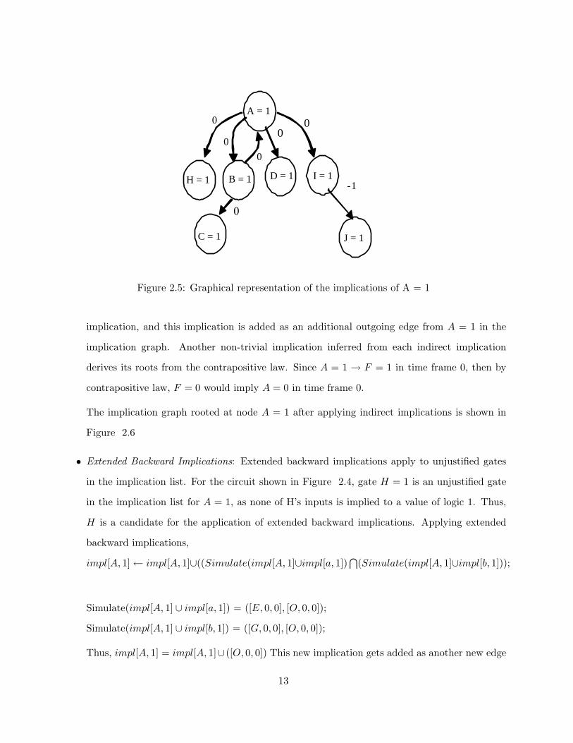
Let us consider the implications of gate A = 1.

• Direct Implications: Direct implications of [A, 1] would be associated with its directly connected

nodes, i.e. gates B, D, I, H. Thus, the set ([A, 1, 0], [B, 1, 0], [D, 1, 0], [I, 1, 0], [H, 1, 0]) forms the

direct implication list for [A, 1]. These implications are stored in the form of a graph as shown

in Figure 2.5

In order to save memory, only the directly connected edges of node A = 1 are stored, and

the complete implication list corresponding to an assignment (say A = 1) is enumerated by

traversing the graph rooted at the node that represents the assignment (i.e. graph is traversed

from node A = 1 to identify impl[A, 1]).

So, traversing the graph shown in Figure 2.5, the implication list for A = 1 after direct

implications would be:

impl[A, 1] = ([A, 1, 0], [B, 1, 0], [D, 1, 0], [I, 1, 0], [H, 1, 0], [C, 1, 0], [J, 1,−1])

• Indirect Implications: Although C = 1 or D = 1 do not imply anything on gate F individually,

together, they imply F = 1. Thus, indirectly, A = 1 would imply F = 1. This is an indirect

12

0

0 0

0

- 1

A = 1

B = 1 I = 1 D = 1 H = 1

J = 1

0

C = 1

0

Figure 2.5: Graphical representation of the implications of A = 1

implication, and this implication is added as an additional outgoing edge from A = 1 in the

implication graph. Another non-trivial implication inferred from each indirect implication

derives its roots from the contrapositive law. Since A = 1 → F = 1 in time frame 0, then by

contrapositive law, F = 0 would imply A = 0 in time frame 0.

The implication graph rooted at node A = 1 after applying indirect implications is shown in

Figure 2.6

• Extended Backward Implications: Extended backward implications apply to unjustified gates

in the implication list. For the circuit shown in Figure 2.4, gate H = 1 is an unjustified gate

in the implication list for A = 1, as none of H’s inputs is implied to a value of logic 1. Thus,

H is a candidate for the application of extended backward implications. Applying extended

backward implications,

impl[A, 1]← impl[A, 1]∪((Simulate(impl[A, 1]∪impl[a, 1])⋂

(Simulate(impl[A, 1]∪impl[b, 1]));

Simulate(impl[A, 1] ∪ impl[a, 1]) = ([E, 0, 0], [O, 0, 0]);

Simulate(impl[A, 1] ∪ impl[b, 1]) = ([G, 0, 0], [O, 0, 0]);

Thus, impl[A, 1] = impl[A, 1]∪ ([O, 0, 0]) This new implication gets added as another new edge

13

0

0 0

0

- 1

A = 1

B = 1 I = 1 D = 1 H = 1

J = 1

0

C = 1

0

F = 1

0

Figure 2.6: Implication graph, after indirect implications

from node A = 1 in the implication graph as shown in Figure 2.7. Also, by contrapositive law,

the implication [O, 1]→ [A, 1] is also learnt.

0

0 0

0

- 1

A = 1

B = 1 I = 1 D = 1 H = 1

J = 1

0

C = 1

0

F = 1

0

O = 0

0

Figure 2.7: Implication graph, after extended backward implications

Note on Extended Backward Implications: As discussed earlier, EB implications are enumerated

for every unjustified gate g in the implication list for a node N . Also, it has been noted that EB

implications require logic simulation for every unspecified input of each unjustified gate. Since the

number of unjustified gates can potentially be of multiple order in magnitude of the size of the circuit,

enumerating EB implications can prove to be expensive in terms of time. However, EB implications

14

cannot be completely ignored because extended backward implications are critical and help discover

many more untestable faults than can be discovered without their enumeration. Thus, it would

be beneficial if the process of identifying EB implications could be carried out only on a subset of

unjustified gates, without incurring any loss w.r.t. the number of untestable faults identified. We

identify such a subset of unjustified gates by performing a check on each unjustified gate before

analyzing the gate for EB implications. The process of identifying a candidate gate for application

of Limited EB implications is described in Figure 2.8.

For every node N{ For every unjustified gate g in the implication list of N

{ For every input i of g { check if the fanin−cone of i has a fanout−stem if fanout−stem does not exist for i { do not perform EB on g break } } }}

Figure 2.8: Algorithm to identify candidate gates for EB implications

The technique described here is new, and helps us reduce the execution time required to create the

implication engine by almost a factor of 1.5-2 for a number of circuits. These results (for sequential

circuits) are shown in Table 2.1.

15

Table 2.1: Comparison of the Limited EB method with the traditional EB method

Circuit Time (sec) Time (sec)

Complete EB Limited EB

s386 0.50 0.36

s400 0.18 0.17

s499 0.72 0.66

s713 0.33 0.28

s953 3.17 2.35

s991 0.42 0.32

s1238 1.10 1.01

s1423 0.35 0.29

s3330 87.41 86.26

s5378 43.25 36.13

s9234 135.41 117.8

s9234.1 62.57 48.79

s13207 238.91 177.6

s13207.1 332.41 260.70

s15850 749.87 414.11

s15850.1 190.69 143.95

s35932 494.64 414.22

s38417 303.24 267.19

s38584 8059.72 1256.89

Results are obtained for an ILA expansion of size 3, i.e. from time frame -1 to 1

16

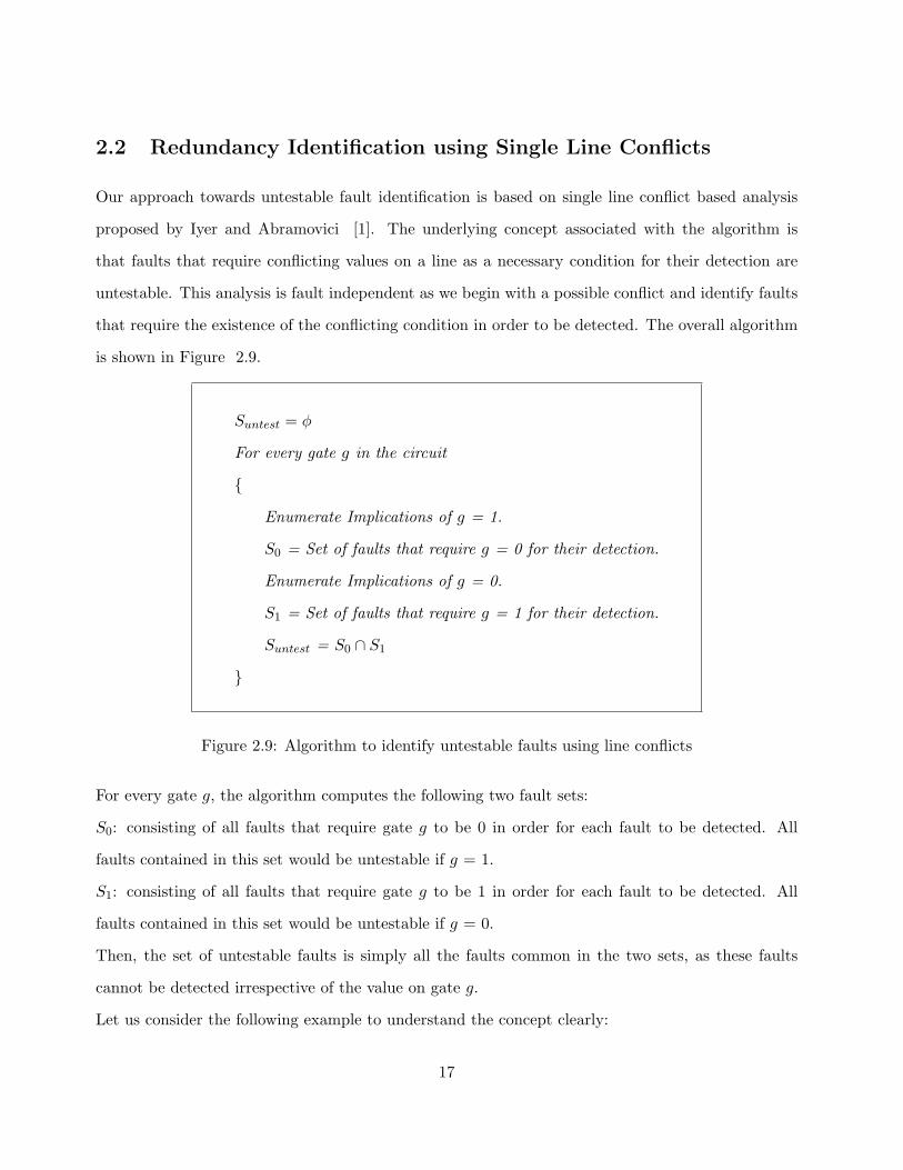
2.2 Redundancy Identification using Single Line Conflicts

Our approach towards untestable fault identification is based on single line conflict based analysis

proposed by Iyer and Abramovici [1]. The underlying concept associated with the algorithm is

that faults that require conflicting values on a line as a necessary condition for their detection are

untestable. This analysis is fault independent as we begin with a possible conflict and identify faults

that require the existence of the conflicting condition in order to be detected. The overall algorithm

is shown in Figure 2.9.

Suntest = φ

For every gate g in the circuit

{

Enumerate Implications of g = 1.

S0 = Set of faults that require g = 0 for their detection.

Enumerate Implications of g = 0.

S1 = Set of faults that require g = 1 for their detection.

Suntest = S0 ∩ S1

}

Figure 2.9: Algorithm to identify untestable faults using line conflicts

For every gate g, the algorithm computes the following two fault sets:

S0: consisting of all faults that require gate g to be 0 in order for each fault to be detected. All

faults contained in this set would be untestable if g = 1.

S1: consisting of all faults that require gate g to be 1 in order for each fault to be detected. All

faults contained in this set would be untestable if g = 0.

Then, the set of untestable faults is simply all the faults common in the two sets, as these faults

cannot be detected irrespective of the value on gate g.

Let us consider the following example to understand the concept clearly:

17

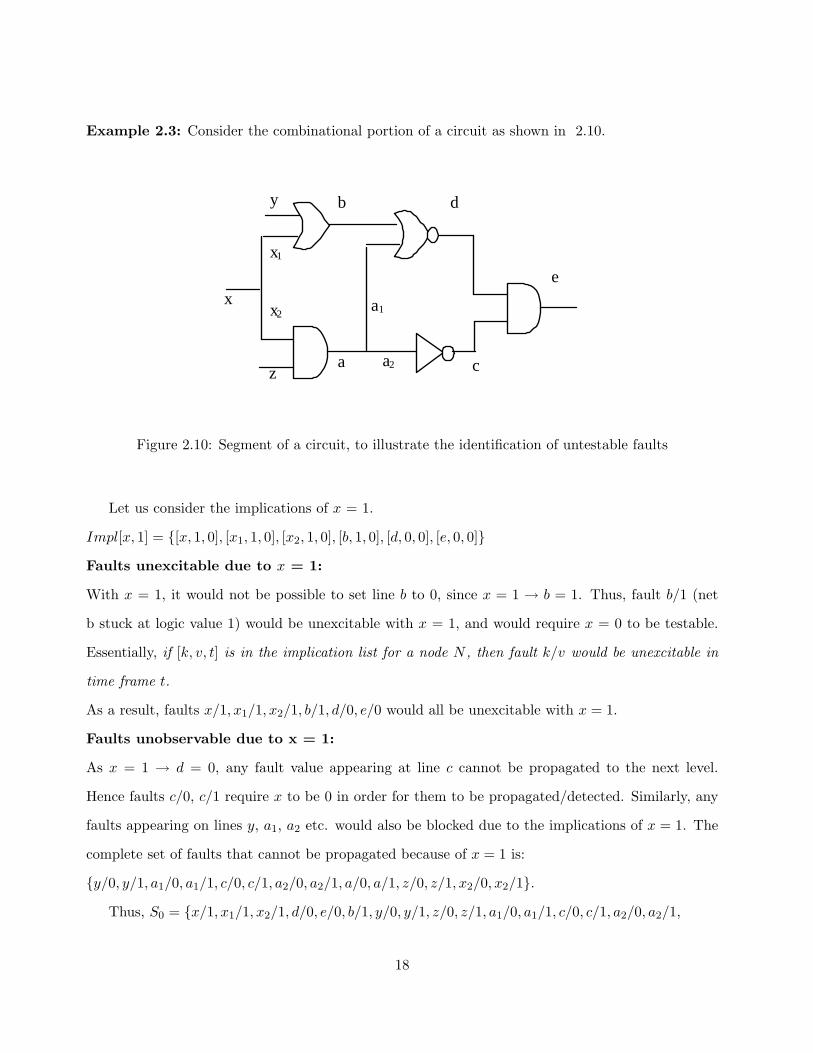
Example 2.3: Consider the combinational portion of a circuit as shown in 2.10.

x x 2

y

a a 2

a 1

x 1

b d

c

e

z

Figure 2.10: Segment of a circuit, to illustrate the identification of untestable faults

Let us consider the implications of x = 1.

Impl[x, 1] = {[x, 1, 0], [x1, 1, 0], [x2, 1, 0], [b, 1, 0], [d, 0, 0], [e, 0, 0]}

Faults unexcitable due to x = 1:

With x = 1, it would not be possible to set line b to 0, since x = 1 → b = 1. Thus, fault b/1 (net

b stuck at logic value 1) would be unexcitable with x = 1, and would require x = 0 to be testable.

Essentially, if [k, v, t] is in the implication list for a node N , then fault k/v would be unexcitable in

time frame t.

As a result, faults x/1, x1/1, x2/1, b/1, d/0, e/0 would all be unexcitable with x = 1.

Faults unobservable due to x = 1:

As x = 1 → d = 0, any fault value appearing at line c cannot be propagated to the next level.

Hence faults c/0, c/1 require x to be 0 in order for them to be propagated/detected. Similarly, any

faults appearing on lines y, a1, a2 etc. would also be blocked due to the implications of x = 1. The

complete set of faults that cannot be propagated because of x = 1 is:

{y/0, y/1, a1/0, a1/1, c/0, c/1, a2/0, a2/1, a/0, a/1, z/0, z/1, x2/0, x2/1}.

Thus, S0 = {x/1, x1/1, x2/1, d/0, e/0, b/1, y/0, y/1, z/0, z/1, a1/0, a1/1, c/0, c/1, a2/0, a2/1,

18

a/0, a/1, z/0, z/1, x2/0}.

Now consider implications of x = 0.

Impl[x, 0] = {[x, 0, 0], [x1, 0, 0], [x2, 0, 0], [a, 0, 0], [a1, 0, 0], [a2, 0, 0], [c, 1, 0]}

Similar to the analysis for x = 1, faults which are unexcitable and unobservable due to x = 0 are

enumerated:

S1 = {x/0, x1/0, x2/0, a/0, a1/0, a2/0, c/1, z/0, z/1}

Thus, S0 ∩ S1 = {x2/0, a/0, a1/0, a2/0, c/1, z/0, z/1} forms the set of faults that are untestable,

because these faults require an impossible (conflicting) assignment on line x as a necessary condition

for their detection.

2.3 Multiple Node Redundancy Identification

The underlying concept of the approach introduced by Gulrajani and Hsiao [8] is also based on

conflict based analysis; however, instead of single line conflicts their approach was based on multiple

node conflicts, where they restricted the number of nodes (over which conflicts are analyzed) to two.

The basic steps used in multiple node redundancy identification are illustrated below:

• Identify a node pair (a, b) for analysis;

• Generate the following implication sets:

– Impl{[a, 0]⋃

[b, 0]};

– Impl{[a, 0]⋃

[b, 1]};

– Impl{[a, 1]⋃

[b, 0]};

– Impl{[a, 1]⋃

[b, 1]};

• Then identify the following four sets of untestable faults:

– S0 = Untestable faults due to Impl{[a, 0]⋃

[b, 0]};

– S1 = Untestable faults due to Impl{[a, 0]⋃

[b, 1]};

– S2 = Untestable faults due to Impl{[a, 1]⋃

[b, 0]};

19

– S3 = Untestable faults due to Impl{[a, 1]⋃

[b, 1]};

• Then identify the set of untestable faults as:

Suntest = {S0⋂

S1⋂

S2⋂

S3}

The faults in the set Suntest would be untestable because they require an impossible combination

of value on nets (a, b). The faults in this set would not be testable for any value combination

of a and b.

However, the selection of candidate pair of nodes is critical, because selecting all node pairs

would make the algorithm’s complexity of order O(n2), and make the whole procedure prohibitively

expensive in terms of time. The author’s of [8] proposed two methods for selecting candidate node

pairs.

In this thesis, we present a new technique to select candidate pair of nodes for multiple node

redundancy identification. We found that our technique for selecting candidate pairs helped us to

identify more untestable faults than could be identified by the algorithm proposed in [8].

2.4 Single Fault Theorem

Single fault theorem [2] was proposed by Agrawal and Chakradhar, as an approach to iden-

tify sequentially untestable faults using combinational ATPG. Before stating the theorem, let us

understand what an iterative logic array (ILA) representation of a sequential circuit refers to.

An iterative logic array expansion of a sequential circuit consists of copies of the combinational

portion of the circuit connected in such a way that the next state generated by the ith copy serves

as the present state variables for the i + 1th copy. Such an ILA expansion of a sequential circuit is

shown in Figure 2.11.

Here, X defines the input bus, Y defines the output bus, Si defines the present state inputs to

the ith time frame, and Ni defines the next state outputs of the ith frame. Lets assume that the initial

state S0 as shown in Figure 2.11 has a reachable state space of size | S0 |. The subsequent reachable

state space for successive time frames shrinks monotonically, i.e. | Si+1 |≤| Si | for 0 ≤ i ≤ k − 1,

where k represents the length of the ILA, i.e. the circuit is unrolled in k frames.

20

C

Y

Y

Y

S 0 S 1 N 0 S k

X X X

C C

Combinational Logic (C)

X Y

N(t) S(t)

f/fs

Y

Figure 2.11: Iterative Logic Array Expansion of a Sequential Circuit

Single Fault Theorem: The single fault theorem states that if a single fault injected in the last

time frame of a k-frame unrolled sequential circuit, i.e. in the kth frame of the ILA, is found to be

untestable using combinational ATPG, then the fault would be sequentially untestable.

The single fault theorem associates the lowest time frame of the ILA with full controllability,

i.e. if the circuit has N flip flops, then the lowest time frame is assumed to have a state space of

2N . Also, the theorem associates the flip-flop boundary in the last time frame of the ILA with full

observability, i.e. the flip-flops in the last time frames behave as primary outputs. So, if a fault effect

propapagtes to the flip-flop boundary in the last time frame, the fault is declared as “ not-untestable”.

In this thesis, we formulate a theorem, which is more powerful than the single fault theorem.

This theorem states that if a single fault injected in any time frame (as opposed to the last time frame

in the single fault theorem) of the k-frame unrolled sequential circuit is found to be untestable (i.e. if

there does not exist a k-frame combinational test for the fault), then the fault would be sequentially

21

untestable too, provided some additional constraints are met. This theorem and its implementation

would be described in detail in the next chapter.

22

Chapter 3

A Novel, Low-Cost Algorithm

In this chapter, we introduce a theorem and a novel, low-cost algorithm to identify sequentially

untestable faults. In the theorem, we state that if a single fault injected in any time frame of the

k-frame unrolled sequential circuit is found to be untestable using combinational ATPG, the fault

would be sequentially untestable, provided some constraints are met. This theorem holds true only if

the target fault either does not re-combine with its copy in a higher time frame, or if re-combination

occurs, the combined fault effect gets blocked. The theorem does not restrict the injection of the

fault in the last time frame (single fault theorem [2] of the ILA, and can handle fault injection in

any time frame. To make the theorem practical, we propose a very inexpensive method of ensuring

that the fault declared as untestable does not become testable after recombining with its own copy

in a higher time frame.

The approach we use is based on an implication engine and the single line conflict analysis similar

to that used in FIRE [1]. Application of the proposed algorithm to ISCAS’89 sequential benchmark

circuits showed that significantly more untestable faults could be identified using our approach, at

practically no computational overhead in terms of both memory and execution time.

3.1 Recombination of Faults

Before discussing the new theorem, we would illustrate that a combinationally untestable fault in

a k-frame unrolled circuit may become testable if the fault effect(s) combine with the same fault in

23

any higher time frame.

Example 3.1: Consider a portion of an unrolled (Iterative Logic Array representation) sequential

circuit shown in Figure 3.1

a/1 E (0/1)

0

0 0

D C B A

1

A B C D

Frame - i Frame i+1

PI

PO

Figure 3.1: ILA representation of a sequential circuit, for two time frames

Consider the fault (we assume a single fault model, i.e. the fault is injected in only one time

frame) a/1 injected in time frame i. Assume that the fault effect for a/1 propagates to the next time

frame as shown in 3.1 (fault effect marked as E). Assuming that the condition that excited the fault

also made the output of gate C equal to logic 0 in time frame i + 1, the fault effect E would seem to

get blocked in time frame i + 1 at gate D. Even though the fault effect got blocked before it could

reach the next time frame or a primary output, the fault cannot be marked as untestable because

the controlling off-path that blocked the fault effect at gate D, contained the gate A itself, indicating

that the injected fault can recombine with its copy in time frame i + 1 and become testable. This

recombination of fault effects is shown in Figure 3.2.

Thus, if we inject a single fault, in order to avoid false positives, where a fault is declared

24

0 /1

E (0/1)

0

0 /1 D C B

A

1

A B C D

Frame - i Frame i+1

0/1

0/1

Figure 3.2: Effect of re-combination of two copies of a fault

untestable wrongly, we must make sure that the fault effect does not recombine with itself in a higher

time frame.

However, just because a fault effect recombines with itself in a higher time frame, it does not

mean that the fault is definitely sequentially testable. For example, assume that gate D is followed

by gate F as shown in Figure 3.3. In this case, the fault effect would be truly blocked at gate F in

time frame i + 1, because the controlling off-path does not contain gate A, and there would be no

chance for the fault to become testable even after recombination. Thus, declaring a fault as testable

just because it recombines with itself in a higher time frame is too conservative, and may lead to a

reduction in the untestable fault list.

Thus, in our approach we guarantee that a fault that we declare as untestable either does not

recombine with itself in any time frame greater than the time frame in which the fault is injected,

or even if recombination occurs, the combined fault effect truly gets blocked. It can be easily seen

that the latter condition is a superset of the former condition. Thus, we present the following cases

which can cause a fault to be sequentially untestable:

25

0 /1

E (0/1)

0

0 /1

D C B A

1

A B C D

Frame - i Frame i+1

0/1

0/1

F F

0

Figure 3.3: Fault effect gets blocked after re-combination

1. If the fault can be excited in some time frame i, but the fault effect cannot be propagated

across the flip-flop boundaries. That is, the fault effect does not reach time frame i+1. (Single

Fault Theorem).

2. If the fault effect crosses time frame boundaries, but does not recombine with a copy of itself

in any higher time frame, and the fault effect is blocked before it can reach either the primary

output or the flip-flop boundary in the last time frame.

3. If the fault effect recombines with itself in a higher time frame, but the combined fault effect

is eventually blocked.

These conditions can be illustrated pictorially as shown in Figure 3.4:

26

A

BC D E

Figure 3.4: Untestable Fault Model

Here, region:

• A: represents combinationally redundant faults.

• B: represents the untestable faults that can be excited (in any time frame), but cannot be

propagated across F/F boundaries. Such faults can be identified using the single fault theorem.

• C: represents those untestable faults that propagate across F/F boundaries, but do not recom-

bine with their own copies in any higher time frames.

• D: Covers the faults lying in region C and also represents those untestable faults that recombine

with themselves in higher time frames, but are eventually blocked.

• E: represents the entire set of sequentially untestable faults.

3.2 Theorem for Sequentially Untestable Fault Identification

In our work, we target the faults that lie in regions C and D. The single fault theorem states

that a target fault injected in the last time frame of a k-frame unrolled circuit, if found untestable,

would be truly sequentially untestable. Our theorem does not restrict the injection of the fault to

27

the last time frame only. The theorem statement is shown below:

Theorem 1: If a target fault injected in any time frame i is found to be combinationally

untestable, and if it can be guaranteed that the injected fault either does not recombine or does

not become testable after re-combination with a copy of the same fault in any time frame greater than

i, the fault would be truly sequentially untestable.

Proof:

Consider the ILA representation of a circuit as shown in Figure 3.5. A k-frame window is selected

to identify untestable faults. For illustration, assume k = 5. Also assume that the fault f is injected

in time frame i, with i = 2, as shown. Faults f1 and f2 represent copies of f in higher time frames.

We also assume the initial state P0, to be fully controllable. If after excitation, the fault effect does

not propagate across the current time frame boundary, then, in accordance with the single fault

theorem, the fault is truly sequentially untestable. However, if the fault effect crosses the current

time frame boundary (crosses time frame 2), then one of the following may occur:

S 0 S 1 S 2 S 3 S 4 S 5

Primary I/ps

Primary o/ps

0 1 2 3 4 5

5 - frame window [time frame 0 – time frame 4]

Shifted 5 - frame window [time frame 1 - time frame 5]

f f 1 f 2

Figure 3.5: ILA representation of a circuit, with a 5-frame window for untestability identification

• Assume that the fault effect f does not recombine with any of its copies (f1 and f2) in any

higher time frame. Since f1 and f2 would not affect the injected fault f , every copy of f for

time frames greater than 2 (i.e. f1 and f2) can be ignored from the perspective of f . If the

28

injected fault f does not propagate to the primary outputs or to the D flip-flops in the last

time frame of the k-frame window (i.e. to S5), then the single fault would be combinationally

untestable. Now we must prove that this fault is the sequentially untestable too. Consider the

same fault injected in a higher time frame i + m. The analysis can be performed simply by

shifting the 5-frame window over which the analysis is performed by m time units. In Figure

3.5, let us consider the same fault injected in time frame 3, so the window would shift by one

time unit and would now extend from time frame 1 to time frame 5. Since the reachable state

space at S1 is a proper subset of the state space at S0, it follows that if the fault injected in

time frame 2 is untestable in the first 5-frame window, the same fault injected in time frame

3 will definitely not be observed over the shifted window as well. This is true for any fault

injected in any time frame because if a fault injected in time frame i gets blocked in time frame

i + m, then the same fault injected in any other time frame (i ± n) would also be blocked in

time frame (i± n) + m. Thus, if the fault injected in any time frame does not recombine with

its own copy in a higher time frame and is found to be combinationally untestable, it would be

sequentially untestable too.

• Assume that the fault effect does recombine with one or more copies of the same fault in a

higher time frame. However, if the combined fault effect gets blocked, then again, fault effects

present in time frames greater than the fault injection frame (i) would not affect the detection

of f . This is true because even though recombination of fault effects occurs, the fault effect

(both combined and single) does not become observable. In order to prove that the fault is

sequentially untestable, we can consider fault injection in any time frame i + m, and shift

the analysis window by m time units. Again, the fault effect would recombine with a copy

in some frame greater than i + m, but the combined fault effect would eventually get blocked

within the analysis window. Thus, if a fault injected in any time frame gets blocked even after

recombination, it would truly be sequentially untestable.

Consider the single fault from the perspective of implications. Assume that there exists a necessary

condition for the excitation of the fault in time frame i. Lets assume that in order to excite the fault

29

a/1 (a stuck-at-1) in time frame i, gate z = 0 in time frame i ± m (where m can be any integer

value) is the necessary condition (because say z = 1 implies a = 1 in time frame i). Assume that

this condition blocks the propagation of the fault in some time frame ≥ i (say p). So, the fault would

be combinationally untestable in the time frame range i to p. However, if it can be guaranteed that,

the fault a/1 does not recombine with any of its copies in any time frame between i and p, then

according to our theorem, the fault would be sequentially untestable. This is so because irrespective

of the value of i, z must be 0 in the time frame i±m if the fault is to be excited. And since z = 0

implies values in the circuit which block the fault in some time frame ≥ i, the fault effect would not

be observable.

3.3 Implementation

Since our implementation is a fault independent one, unlike the implementation of the single fault

theorem, we do not inject any fault in the circuit. We use the concept of the theorem we presented as

a guide to find more untestable faults using an implication engine and the single line conflict (FIRE)

algorithm.

Whenever any input(s) to a gate is a controlling value for the gate, all the other inputs become

unobservable because values present at these inputs would be blocked by the controlling value present

at the other input. This unobservability propagates along the input cone of each of the ‘unobservable

lines/inputs’. The concept of unobservability propagation is shown in Figure 3.6.

Whenever a stem is encountered in this unobservable cone, an analysis is done to determine if all

branches of the stem are unobservable (blocked). If even one branch is found to be observable (un-

blocked), the stem is marked observable, and unobservability does not propagate beyond (backwards

from) this stem. This analysis is in accordance with lemma 1 [1] introduced in FIRE. However,

we take special care when this unobservability cone extends beyond time frame boundaries. This

is required to prevent declaring a signal as unobservable, when it actually becomes observable after

re-combining with itself in a higher time frame. As stated in the theorem, if it can be guaranteed

that a signal/fault does not re-converge with itself in a higher time frame or does not become ob-

30

D C B

A 0 Unobservability cone.

No signal in this cone is observable due to the controlling value present at one of D’s inputs

Figure 3.6: Unobservability Cone

servable/testable even after recombination, it can safely be marked as unobservable or untestable.

Thus, we propagate unobservability backwards across time frame boundaries, and declare a signal as

unobservable only if it is truly unobservable in accordance with our theorem. The key is to develop

a technique that would determine if a signal is truly unobservable (even after recombination) or

not, without causing extra overhead in terms of both execution time and memory requirements. We

achieve this by performing a special stem analysis in a sequentially unrolled circuit. The concept

can be better understood through the following example.

Example 3.2: Consider the circuit shown in Figure 3.7. Let us assume that the implications of

a node, say z = 0, are as shown in 3.7 ([C, 1, i], [B, 0, i+1], etc). The presence of a controlling value

at the input of D in time frame i+1 (due to C = 0) would cause the input cone associated with the

other input to become unobservable. Assuming that the unobservability propagates across the time

frame boundaries, we would need to analyze the observability of the stem at the output of gate A in

time frame i. The following steps are undertaken for this analysis:

1. We associate an ID (say X) with gate A in time frame i, and propagate it. X can propagate

across B, but would be blocked by the controlling value present at the off-path input of C.

Since there is another path for the ID to propagate (dashed path), the stem cannot be declared

31

0

0 0 D C B

A

1

A B C D

1 1

X X

X X

Y

Y

Y

Z Z

Figure 3.7: Two-frame ILA to demonstrate ID propagation for unobservability analysis

as unobservable at this stage. Let us assume that the ID, X, propagates to a D flip flop, and

crosses the time frame boundary.

2. Before we start analyzing the propagation path for ID X, we associate gate A (the gate from

which ID propagation began in time frame i) with a new ID (say Y ) in time frame i + 1, and

propagate it, until it gets blocked in the current time frame (i.e. time frame i + 1). Here, Y

would propagate across gate B, gate C and gate D.

3. Now we analyze the path of the previous ID, i.e. X associated with time frame i. The ID

propagates to D. Although the other input to gate D presents a controlling value, the ID

associated with this controlling input is Y , implying that there exists a path for the fault at

gate A in time frame i to combine with the fault present at gate A in a higher time frame. Thus,

the stem is not declared as unobservable, and ID X propagates across gate D in time frame

i + 1. If there is another gate at the output of D, say E, with the other input(s) controlling

the output, then the ID at the output of D would truly be blocked (assuming that the other

controlling input(s) of E cannot be reached by either A in time frame i + 1 or by A in time

frame i).

32

3.4 Algorithm

The complete algorithm for untestable fault identification is shown in Figure 5.7.

The implication graph (explained in Chapter 2) is generated as a pre-processing step to untestable

Generate the Implication graph using:

Direct, Indirect and Extended Backward Implications.

//Perform single line conflict analysis with the addition

//of extended unobservability propagation.

Suntestable = φ;

For every gate g in the circuit

{

Enumerate Implications of g = 1.

S0 = Set of faults that require g = 0 for their detection.

Enumerate Implications of g = 0.

S1 = Set of faults that require g = 1 for their detection.

Propagate unobservability across time frame boundaries when required.

Suntestable = S0 ∩ S1

}

Figure 3.8: Algorithm to identify untestable faults using the application of the new theorem

fault identification. Initially, a graph consisting of direct implications is generated. Indirect and

extended backward implication are then enumerated for each gate and added to the implication graph.

However, extended backward implications are enumerated for only a subset of unjustified gates for

each node in the implication graph. The way the candidate gates are chosen was explained in Chapter

2. Single line conflict algorithm is then applied to identify untestable faults. The new theorem is

applied wherever applicable to extend the unobservability cone across time frame boundary. This

33

propagation of unobservability across time frame boundaries increases the probability of identifying

more untestable faults, because now, a bigger intersection can be achieved between sets S0 and S1

(Figure 5.7).

3.5 Results

The proposed algorithm was implemented in C++ and experiments were conducted on ISCAS89

and ISCAS93 circuits on a 1.8 GHz, Pentium-4 workstation with 512 MB RAM, with Linux as the

operating system. The results are reported in Tables 5.1 and 5.2. In Table 5.1, results were

obtained for two implementations for each circuit. The first implementation (traditional method)

did not consider the newly proposed theorem, and here, the unobservability propagation does not

cross time frame boundaries. The second implementation, based on the proposed method, did not

bound unobservability propagation to time frame boundaries, and we made sure that recombination

of fault effects would not cause false positives via our theorem and algorithm. Since the implication

graph for both the traditional and our approaches are exactly the same, the memory requirements

are identical. For the traditional implementation, the untestable fault set Suntest, and execution time,

are reported for time frames ranging from -1 to 1 (M or Maximum Edge Weight = 1) in columns

2 and 3 of Table 5.1 and for time frames ranging -5 to 5 (M = 5) in columns 4 and 5. For the

second implementation, which involves the implementation of our theorem, the implication graph is

generated only over time frame range -1 to 1, and the set of untestable faults Suntest identified and

the corresponding execution times are reported in columns 5 and 6 in Table 5.1. It can be seen that

for many circuits, our proposed approach could identify more untestable faults without too much

additional computational effort.

For example, in s5378, the proposed theorem could identify 877 untestable faults in only 46.02

seconds (with time frames ranging -1 to 1), while the traditional implementation could identify only

778 untestable faults over the same time frame range of -1 to 1, in 45.04 seconds. Even when the

ILA size is increased to 11 (time frame -5 to 5), only 781 untestable faults were identified with the

traditional method, at a cost of more than 900 seconds. This indicates that increasing the ILA size

by the traditional method cannot capture untestable faults that recombine within the ILA. Note

34

Table 3.1: Untestable Faults Identified (New Theorem vs Traditional Implementation)

Traditional Implementation New Approach

Circuit Suntest Time Suntest Time Suntest Time

∗M = 1 (sec) M = 5 (sec) M = 1 (sec)

s386 60 0.41 60 0.70 60 0.4

s400 7 0.17 8 0.73 8 0.26

s499 89 0.85 89 6.99 89 0.89

s713 32 0.29 32 0.58 32 0.34

s953 4 2.98 4 6.34 4 3.58

s991 0 0.40 0 1.35 6 0.40

s1238 9 1.17 9 1.45 9 1.66

s1423 9 0.35 9 1.04 9 0.42

s3330 420 88.6 420 112.77 493 88.94

s5378 778 39.47 781 732.75 877 42.07

s9234.1 193 69.71 193 155.17 195 90.80

s13207.1 374 273.78 381 1036.6 399 290.74

s15850.1 315 155.77 315 902.76 317 194.5

s35932 3984 435.19 3984 772.60 3984 487.65

s38417 328 336.58 332 2442.95 356 681.95

s38584 1638 1369.9 1654 5938.66 1691 1551.72

∗M : Maximum Edge Weight: M = 1→ frame range from -1 to 1

35

that our approach only required less than 1 seconds (in same ILA size) to perform unobservability

propagation across time frame boundaries and detected nearly 100 more untestable faults. Likewise,

for s3330, 73 more untestable faults were identified at practically no overhead. Not only does the

implementation based on our new theorem identify more untestable faults without costing much

additional effort, it also does not require additional memory overhead. For some circuits (s9234.1,

s15850.1, etc), the number of untestable faults identified using the new method was the same as those

identified using the traditional approach. For these circuits, crossing the time frame boundaries did

not benefit in identifying more untestable faults. Here, an implementation based on the single fault

theorem would be sufficient to identify untestable faults, because faults injected in a time frame i that

cross time frame boundaries do not get blocked in higher time frames with or without recombination

with multiple copies of the same fault. Table 5.2 compares our results with the untestable fault set

obtained using FUNI+FIRE [11].

Here, column 2 shows the number of untestable faults identified by the combination of FUNI

and FIRE, when run on SUN sparc10 [11]. The column shows two quantities: number of untestable

faults identified / number of time frames the sequential circuit was unrolled into. Column 3 shows the

corresponding execution times. Column 4 through 7 show the number of untestable faults identified

by our tool, using only 3 frames for all circuits, and the time taken for the analysis, respectively.

We report results for 2 scenarios: with and without extended backward (EB) implications (since

FUNI+FIRE did not use EB implications). It can be seen that although our tool does not explicitly

enumerate a subset of the illegal state space, we can identify more untestable faults as compared

to FUNI and FIRE combined, for quite a few circuits. FUNI outperforms our implementation for

circuits which have a lot of un-initializable flip flops (such as s15850), and hence a lot of unreachable

states. Since we do not enumerate unreachable states, we identify a smaller subset of untestable

faults for these circuits. Note that for most circuits, we can identify more untestable faults using

fewer number of frames. Finally, even when the tool is run without EB implications, we still identify

a larger subset of untestable faults for a few circuits.

36

Table 3.2: Comparison of our tool with FUNI+FIRE

FUNI+FIRE Our Tool Our Tool

(W/O EB Impl) (W/ EB Impl)

Circuit Suntest/ Time Suntest/ Time Suntest/ Time

#Fr. (sec) #Fr. = 3 (sec) #Fr. = 3 (sec)

s386 36/2 0.4 60 0.11 60 0.4

s400 16/3 2.0 8 0.42 8 0.26

s713 91/15 1.7 32 0.11 32 0.34

s953 0/5 8.5 4 1.20 4 3.58

s1238 6/3 4.1 6 0.85 9 1.66

s1196 0/3 3.5 0 0.32 0 0.96

s1423 5/2 12.3 9 0.25 9 0.42

s5378 414/15 43.5 577 4.79 877 42.07

s9234 257/15 108.8 272 43.95 274 163.41

s13207 654/10 150.8 688 29.06 791 197.74

s15850 816/10 114.0 356 78.1 445 479.16

s35932 3984/0 237.4 3984 80.47 3984 487.65

s38417 381/5 373.4 337 297.1 356 681.95

s38584 1582/5 405.4 1553 333.8 1691 1551.72

37

Chapter 4

Multiple Node Conflict Analysis

This chapter describes a multiple node redundancy identification algorithm which can be used

to identify more untestable faults than the single line conflict analysis can identify. This work is

motivated by the analysis presented by Gulrajani and Hsiao [8]. Although our approach is based

on the concept introduced in [8], the way we identify a candidate node pair for analysis is different

from the selection methods introduced earlier. Also, the work presented in [8] is limited to com-

binational circuits, while the work presented here is applicable to sequential circuits as well. Also,

we observed that by using a different technique to identify candidate node pairs, we could identify

more untestable faults than the methods in [8] could identify, and in better time. The basic idea

is to find a candidate pair of node [a, b], and identify faults that require a conflicting (assignment)

combination of values on these gates, as a necessary condition for their detection. However, if the

circuit has n gates, then the number of such candidate pairs could be of the order of n2, i.e. if all

gates are paired up. If we assume that such an exhaustive search identifies m extra untestable faults,

then the idea is to reduce n to n1 (such that n1 � n) without letting a reduction occur in m.

38

The basic algorithm is described below:

• Identify a node pair (a, b) for analysis;

• Generate the following implication sets:

– Impl{[a, 0]⋃

[b, 0]};

– Impl{[a, 0]⋃

[b, 1]};

– Impl{[a, 1]⋃

[b, 0]};

– Impl{[a, 1]⋃

[b, 1]};

• Then identify the following four sets of untestable faults:

– Set0 = Untestable faults due to Impl{[a, 0]⋃

[b, 0]};

– Set1 = Untestable faults due to Impl{[a, 0]⋃

[b, 1]};

– Set2 = Untestable faults due to Impl{[a, 1]⋃

[b, 0]};

– Set3 = Untestable faults due to Impl{[a, 1]⋃

[b, 1]};

• Then identify the set of untestable faults as:

Suntest = {Set0⋂

Set1⋂

Set2⋂

Set3}

4.1 Identification of Candidate Node Pairs

The basic approach we use to identify candidate node pairs is described below:

• Identify all stems S1, S2, ..., Sn that reconverge on the same gate g (A stem or a fanout-stem is

defined as a circuit element that has more than one fanout).

• Identify the distance in terms of multiple input gates between these stems and gate g.

• Create a link from gate g to all stems that re-converge on g with a distance less than some

threshold.

39

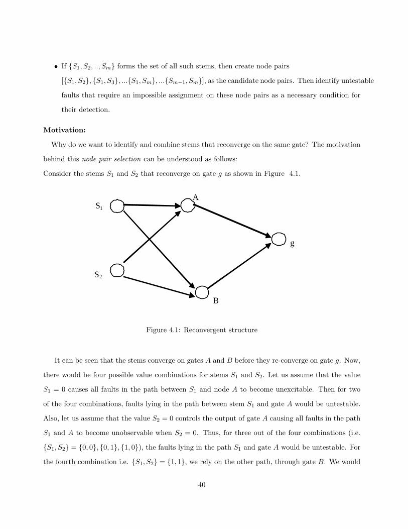
• If {S1, S2, .., Sm} forms the set of all such stems, then create node pairs

[{S1, S2}, {S1, S3}, ...{S1, Sm}, ...{Sm−1, Sm}], as the candidate node pairs. Then identify untestable

faults that require an impossible assignment on these node pairs as a necessary condition for

their detection.

Motivation:

Why do we want to identify and combine stems that reconverge on the same gate? The motivation

behind this node pair selection can be understood as follows:

Consider the stems S1 and S2 that reconverge on gate g as shown in Figure 4.1.

S 1

S 2

A

B

g

Figure 4.1: Reconvergent structure

It can be seen that the stems converge on gates A and B before they re-converge on gate g. Now,

there would be four possible value combinations for stems S1 and S2. Let us assume that the value

S1 = 0 causes all faults in the path between S1 and node A to become unexcitable. Then for two

of the four combinations, faults lying in the path between stem S1 and gate A would be untestable.

Also, let us assume that the value S2 = 0 controls the output of gate A causing all faults in the path

S1 and A to become unobservable when S2 = 0. Thus, for three out of the four combinations (i.e.

{S1, S2} = {0, 0}, {0, 1}, {1, 0}), the faults lying in the path S1 and gate A would be untestable. For

the fourth combination i.e. {S1, S2} = {1, 1}, we rely on the other path, through gate B. We would

40

want this combination to generate a new implication on gate B which can reach gate g and make

the other path, i.e. through gate A unobservable. This would make faults lying in the path between

stem S1 and gate A unobservable, and hence untestable because they cannot be detected for any

combination of values associated with stems S1 and S2.

However, the greater the number of multiple input gates between the stem-pair and the re-

convergent gate, lesser would be the probability that any implication associated with either of the

stems would reach the re-convergent gate. For example, if there were a lot of multiple input gates

between stem S2 and gate g (through the path that contains gate B), then the probability that the

new implication generated through the combination {S1, S2} = {1, 1} would reach the re-convergent

node would be less. Hence the last combination of {1, 1} would not make the faults lying in the

path from stem S1 and gate A unobservable. Therefore, not all reconvergent stem-pairs would be

useful. So, we filter out some stem-pairs by identifying the distance (in terms of multiple input gates)

between the stem under consideration and its re-convergent gate.

Consider what would happen if (refer Figure 4.1) there are a lot of multiple input gates between

either stem S1 and gate A or between stem S2 and gate A. If there exist a lot of multiple input gates

between stem S2 and gate A, then it is possible that the assignment S2 = 0 gets blocked midway

and does not propagate through to gate A. This would mean that the combination {S1, S2} = {1, 0}

would no longer make the path between stem S1 and gate A unobservable indicating that the faults

lying in the path can no longer be marked as untestable. Also, if the distance in terms of multiple

input gates between stem S1 and gate A is high, then the assignment S1 = 0 may not make a lot of

nets unexcitable as the value assignment may get blocked early. Thus, if we want to combine stems

S1 and S2, then we must make sure that:

• Check #1: The number of multiple input gates between stems S1 and S2 and the reconvergent

gate is below a threshold (say threshold1);

• Check #2: The number of gates between S1 and the gate(s) at which S1 converges with S2

is less than a given threshold (say threshold2). Also, the number of gates between S2 and the

gate(s) at which the two stems converge is less than the threshold (i.e. less than threshold2).

41

After a lot of experimentation, in our analysis, we’ve set threshold1 to 10 gates, and threshold2

to 4 gates. It is also important to note that there would be no point in combining stems that have

less than 2 overlapping paths to the convergent node. Thus, we combine stems S1 and S2 if and only

if they have atleast 2 overlapping or common paths to the reconvergent gate.

Although it is beneficial to prune out the number of stems to be combined, it is important

that the pruning scheme not be very expensive in terms of time. However, the pruning scheme which

involves estimating the distance between the candidate stems and the gates on which they converge

(i.e. Check #2) can prove to be very expensive if carried out on all stem pairs. Thus, we use an

intuitive concept to eliminate candidate pairs before performing Check #2. The concept we use is

based on the fact that stems which are structurally far apart in the circuit may not converge early,

and hence one or more combination of values (from the set {0, 0}, {0, 1}, {1, 0}, {1, 1}) would not

generate any untestable faults (which would mean that the intersection of set Set0, Set1, Set2, Set3

may turn out to be null). That is, if assume that stems S1 and S2 form a candidate node pair and

these two stems are structurally far apart in the circuit, then, one of these stems would potentially

have a lot of multiple input gates in its path before it can converge with the other stem. Thus, it

would not be beneficial to combine these two stems for analysis. So, we perform Check #2 only on

stems that are structurally close, and do not combine stems which are structurally distant.

We use two metrics to determine if two stems are structurally close or not. The first metric is the

forward level of the stem, which indicates how far the stem is from primary inputs, and the other

metric is the backward level, which indicates how far the stem is from a primary output. After

performing a lot of analysis, we found that only the candidate pair of stems which are either in

the same backward level or in the same forward level are useful in terms of identifying additional

untestable faults, and stems which do not lie either in the same forward level or in the same backward

level generally tend to be structurally spaced, and do not converge soon.

Thus, the overall algorithm to identify candidate node pairs can be described as shown in Figures

4.2 and 4.3.

42

Table 4.1: Performance of the multiple node FIRE w.r.t. the single line FIRE

Single line FIRE Multi-Node FIRE

Circuit Suntest Time (sec) Suntest Time (sec)

c2670 39 0.65 81(+42) 6.97

c3540 105 3.74 130(+25) 90.16

c5315 20 2.12 32(+12) 10.19

c7552 42 8.76 54(+12) 81.93

s386 60 0.4 64(+4) 0.82

s400 8 0.26 10(+2) 0.33

s713 32 0.34 38(+6) 0.45

s953 4 3.58 5(+1) 5.75

s1238 9 1.66 17(+8) 4.90

s1423 9 0.42 11(+2) 0.80

s5378 877 42.07 883(+6) 126.20

s9234.1 195 90.80 299(+104) 208.24

s13207.1 397 290.74 410(+13) 956.38

s15850.1 317 194.5 336(+19) 815.96

s38417 356 681.95 393(+37) 1301.36

s38584 1691 1551.7 1781(+90) 4341.43

Results are obtained for an ILA expansion of size 3, i.e. from time frame -1 to 1

43

4.2 Results

The proposed algorithm was implemented in C++ and experiments were conducted on ISCAS85

and ISCAS89 circuits on a 1.8 GHz, Pentium-4 workstation with 512 MB RAM, with Linux as the

operating system. The results obtained (number of untestable faults identified Suntest and execution

time) for the multiple node FIRE are presented in Table 4.1. Column 1 in Table 4.1 lists the combi-

national and sequential circuits for which the algorithm was evaluated. Column 2 shows the number

of untestable faults identified using the single line conflict approach coupled with the theorem intro-

duced in Chapter 3. Column 3 lists the respective execution times. Columns 3 lists two quantities.

The first value is the number of untestable faults identified using the multiple node conflict analysis

(after having run the single line FIRE) and the second value in the parenthesis is the number of

untestable faults identified in addition to the number identified by single line FIRE. Finally, column

5 shows the time taken to run the entire tool (i.e. the time taken to build the implication graph,

to execute single line FIRE and the time taken to execute the multiple node FIRE). For example,

for circuit c2670, the single line FIRE could identify 39 untestable faults in 0.65 seconds, while the

multiple node FIRE could identify an additional 42 untestable faults in a total time of 6.97 seconds.

It can be seen that the multiple node analysis could identify a significantly larger set of untestable

faults as compared to the single line FIRE for most of the circuits, but at a higher cost in terms of

run time.

Table 4.2: Comparison of the technique proposed in [8] with our technique

Previous Method [8] New Multi-Node FIRE

Circuit Suntest Time (sec) Suntest Time (sec)

c432 1 0.18 0 0.22

c2670 44 31.0 81 6.97

c3540 115 427.0 130 90.16

c5315 20 - 32 10.19

c7552 44 357.8 54 81.93

44

Table 4.2 compares the results obtained by our technique with the results obtained by the

technique proposed by Gulrajani and Hsiao [8]. Since they ran their tool only for combinational

circuits, results for sequential circuits are omitted here. The first column shows the circuits for which

the tools were executed. The second and the third columns show the number of untestable faults

identified and the time taken (respectively) by the method proposed in [8]. Finally, the fourth and

the fifth columns show the number of untestable faults and the execution times for our multi-node

analysis technique. The experiments by Gulrajani [8] were conducted on a UltraSPARC-1 station

with 64MB RAM. It can be seen that we can identify more untestable faults with the proposed

technique of selecting node pairs. Also, the time we spend on the analysis is less than 1/3rd of the

execution times reported in [8].

45

For every stem S in the circuit

{

Identify the gate G on which S reconverges.

Determine the distance d between S and G in terms

of multiple input gates.

If d ≤ threshold1, create a link from G to S.

}

For every reconvergent gate G with m (m ≥ 2) outgoing links

{

For all links from i to m

{

Identify Si and Si+1 as a candidate node pair.

If Si and Si+1 lie in the same forward or backward level

{

• check2 = combinationCheck(Si, Si+1)

• if (check2 = 1)

• Combine stem Si and Si+1 to

identify additional untestable faults.

}

}

}

Figure 4.2: Algorithm to identify candidate stem pairs for multiple gate redundancy analysis

46

combinationCheck(S1, S2)

{

• Identify the gates on which S1 and S2 converge.

• If Si and S2 converge on less than 2 gates,

return 0.

• Determine the distance between S1 and the gates on which

it converges with S2.

• If distance is greater than threshold2 return 0.

• Determine the distance between S1 and the gates on which

it converges with S2.

• If distance is greater than threshold2 return 0.

return 1

}

Figure 4.3: Function to perform Check #2 on candidate stem pairs

47

Chapter 5

Implications based Untestable Bridge

fault Identifier

In this chapter, we present novel, low cost technique based on implications to identify untestable

bridging faults in sequential circuits. Sequential symbolic simulation [12] is first performed, as a

preprocessing step, to identify nets which are uncontrollable to a specific logic value. Then, an

implication-based analysis is carried out for each fault to determine if a particular fault is testable

or not. We also use information about the untestable stuck-at faults to filter out some bridges early

in the analysis process. The application of our technique to ISCAS 89 sequential benchmark circuits

and a few industrial circuits showed that a large number of untestable bridges could be identified at

a low cost, both in terms of memory and execution time.

5.1 Introduction

A bridge fault between two or more nets refers to a defect where the nets are unintentionally

shorted together. While the size of the more commonly studied stuck-at fault list is of the order of

the size of the circuit, bridging fault lists can potentially be of polynomial order in the size of the

circuit. Furthermore, the cost of bridge-fault ATPG can exceed that of the stuck-at counterpart.

Thus, it would be beneficial to quickly identify bridging faults that are redundant/untestable, so that

tools such as bridging fault ATPG engines or bridging fault simulators do not waste time targeting

48

these faults. Our work focuses on efficient identification of such untestable bridging faults.

Algorithms have been proposed earlier for two node [13] and multinode [14] bridge fault

extraction/analysis. In our approach, we limit the analysis to two-node bridges. Also, we assume

the bridge fault to be present between the outputs of two nodes, and no bridges internal to a Boolean

gate are considered for analysis. Resistance of a bridge determines the kind of fault effect the bridge

produces in a circuit. Bridges of high resistance type cause the outputs of the succeeding gates to

have a delayed transition, leading to a delay fault, while bridges having low resistance (hard short)

cause the static behavior of the circuit to change. In our analysis, we assume the bridge fault to

be of the hard short type, which causes the functionality of the circuit to change. A lot of models

have been proposed for the analysis of such kind of bridges. Stuck-at faults have been used to

model the behavior of bridges [15], along with the voting [16] and the biased voting method [17],

which are the more popular modeling methods. The model we use for our purpose of identifying

untestable bridges is based on the wired and the dominant fault models [18]. Although much

work has been presented for the identification of untestable stuck-at faults, there hasn’t been any

significant contribution towards the identification of untestable bridges in sequential circuits. Thus,

to the best of our knowledge, our work on the identification of untestable bridges using implications

is the first of its kind. Our implementation is based on the representation of a sequential circuit as

an iterative logic array (ILA) of fixed length. For each bridge, we identify a set of conditions that

are necessary for the fault to be testable. We imply these set of conditions within the ILA and use

this information to determine whether the bridge can be declared as untestable or not. We evaluated

our tool against the larger ISCAS 89 circuits along with a few industrial circuits. We validated

and compared these results with our internal ATPG engine for bridging faults. Interestingly, it was

observed that we could identify more untestable faults using this new tool than the ATPG tool could

identify. The relationship between the untestable faults identified by the ATPG tool and our new

implications based tool is shown in 5.1

Although the graphical representation of implications proposed in [9] is a memory efficient

approach, it would still blow up for large (sequential) industrial circuits (with size > 100K gates).

Also, the use of extended backward implications on such circuits would prove to be too expensive

49

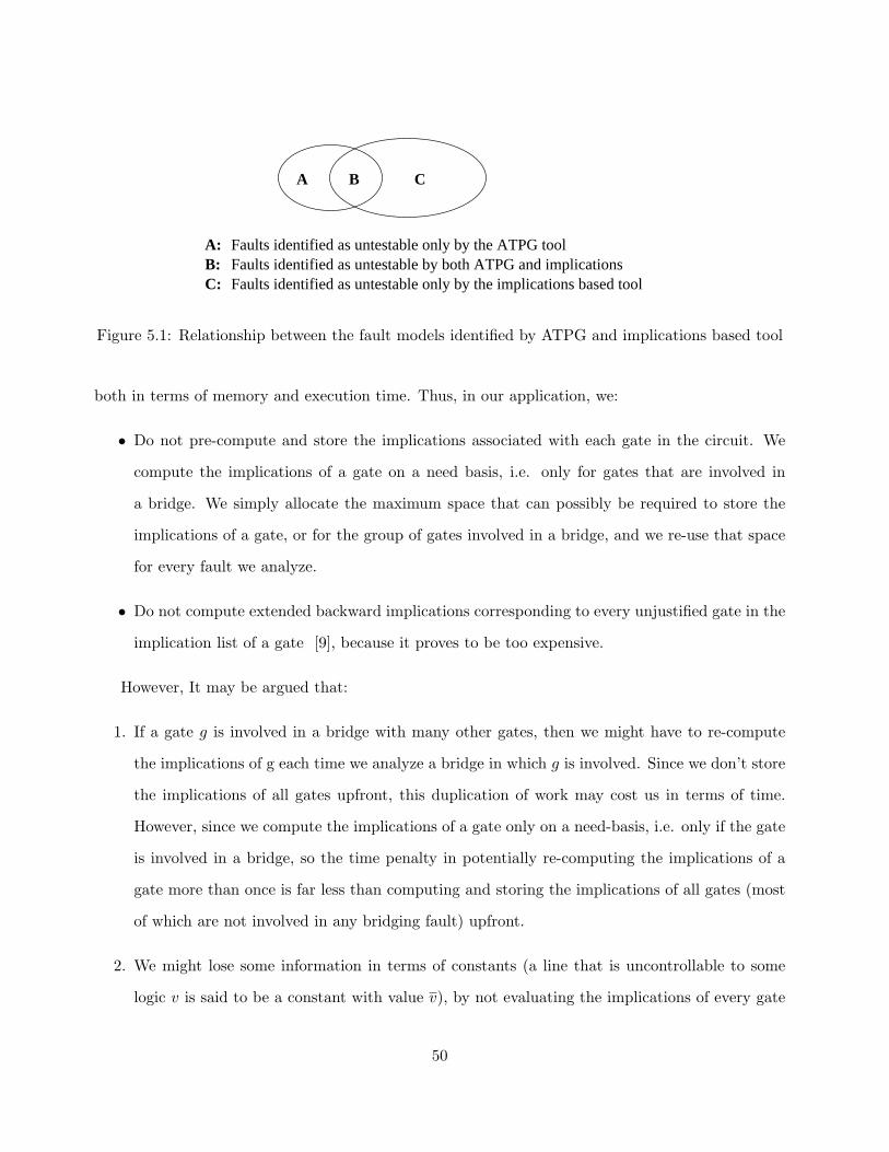
A B C

A: Faults identified as untestable only by the ATPG toolB: Faults identified as untestable by both ATPG and implicationsC: Faults identified as untestable only by the implications based tool

Figure 5.1: Relationship between the fault models identified by ATPG and implications based tool

both in terms of memory and execution time. Thus, in our application, we:

• Do not pre-compute and store the implications associated with each gate in the circuit. We

compute the implications of a gate on a need basis, i.e. only for gates that are involved in

a bridge. We simply allocate the maximum space that can possibly be required to store the

implications of a gate, or for the group of gates involved in a bridge, and we re-use that space

for every fault we analyze.

• Do not compute extended backward implications corresponding to every unjustified gate in the

implication list of a gate [9], because it proves to be too expensive.

However, It may be argued that:

1. If a gate g is involved in a bridge with many other gates, then we might have to re-compute

the implications of g each time we analyze a bridge in which g is involved. Since we don’t store

the implications of all gates upfront, this duplication of work may cost us in terms of time.

However, since we compute the implications of a gate only on a need-basis, i.e. only if the gate

is involved in a bridge, so the time penalty in potentially re-computing the implications of a

gate more than once is far less than computing and storing the implications of all gates (most

of which are not involved in any bridging fault) upfront.

2. We might lose some information in terms of constants (a line that is uncontrollable to some

logic v is said to be a constant with value v), by not evaluating the implications of every gate

50

in the circuit. However, we more than compensate for this through the sequential symbolic

simulation.

3. By not performing extended backward implications, we might not have as powerful an im-

plication engine, as we might have with the application of extended backward implications.

Though this is true, the time penalty associated with the computation of extended backward

implications for every unjustified gate in the implication list for a gate outweighs the advantage

of a more powerful implication engine available with extended backward implications.

5.2 Symbolic Simulation

Symbolic simulation is performed as a preprocessing step to untestable bridge analysis; it identifies

nets that are uncontrollable to a specific logic value. For example, line b in the circuit shown in 5.2

is uncontrollable to logic 0 assuming that the initial state of the flip-flop is unknown, and line a is

fully controllable to any value.

b

D

a Q

CLK

Figure 5.2: Illustration of uncontrollability

We perform symbolic simulation using 11 symbols, that represent the controllability charac-

teristics of any given line. Node G is uncontrollable to a logic value V means: There is no single

finite sequence I, which when applied to the controllable points in the net-list, can set G to value V

for every possible power up state of the sequential elements in the design, where V ∈ {0, 1, Z} . Z in

the value set refers to the high impedance state of a net. Since most of the industrial circuits have

51

tri-state devices and bus structures, we support the high impedance value in our tool. The symbols

used, and their meaning is described below:

• Strong 0 (Strong 1): If a line can only take a value of strong0 (strong1), then it is associated

with this symbol. For example, a net directly connected to VSS (VDD) would take this symbolic

value. (Represented as ST 0(ST 1)).

• ControllableToAny (C ANY ) : If a particular net can assume any value from the defined

value set, then it is associated with the ControllableToAny symbol. This symbol is associated

with all the primary inputs and the scan elements.

• UncontrollableTo 0 (UncontrollableTo 1): A net that cannot be controlled to logic 0 (logic

1) is associated with the UncontrollableTo 0 (UncontrollableTo 1) symbol. For example, the

output of the OR gate shown in 5.2 cannot be driven to logic 0, and hence would assume this

symbol. (Represented as UN 0 (UN 1)).

• UncontrollableToAny (U ANY ): This symbol is associated with the net that cannot be con-

trolled to any value. This is the symbol associated with the output of every non-scan latch/flip-

flop at the beginning of symbolic simulation.

The symbolic values described above can be associated with any gate/net in the circuit, while the

ones described below can only be associated with the nets that produce/transmit a high impedance

(Z) state.

• Strong Z : Associated with the net that can only take the high impedance state. For example,

a tri-state device with an active high enable would assume this symbolic value, if the enable

line is a constant 0.

• UncontrollableTo Z: A net would assume this value if it can never achieve the high impedence

state. For example, a controlled buffer with an active high enable would be associated with

this symbolic value if the enable line is a constant 1.

• UncontrollableTo 01: If a net can never be driven to either 0 or 1, then it would be associated

with this symbolic value.

52

• UncontrollableTo 1Z: A net which cannot achieve either a high impedance state or cannot be

excited to logic 1 would be associated with this symbolic value. For example, a wired-AND

gate (as shown in Figure 5.3) with one driver set at UncontrollableTo 1Z would be associated

with this symbolic value, as the UncontrollableTo1Z on one of the driver’s o/p would dominate

the value on any other driver.

Wired - AND gate UncontrollableTo_1Z

UncontrollableTo_1Z

Figure 5.3: Illustration of symbolic value UncontrollableTo 1Z

• UncontrollableTo 0Z: A net which cannot be excited to either a logic value of 0 or Z would

be associated with this symbolic value. For example, a wired-OR gate with one driver as

UncontrollableTo 0Z would be associated with the symbolic value of UncontrollableTo 0Z

(as shown in Figure 5.4).

Wired - OR gate UncontrollableTo_0Z

UncontrollableTo_0Z

Figure 5.4: Illustration of symbolic value UncontrollableTo 0Z

Symbolic simulation is initiated by assigning ControllableToAny symbol to all primary

inputs and scan elements, and UncontrollableToAny symbol to all latch elements/flip flops. The

53

simulation is event-driven; it proceeds in a levelized manner, and each gate is evaluated one time

frame after another, until the circuit settles down to a stable state. To propagate symbols, pre-

computed characteristic propagation table for each gate is looked up to determine the resulting

symbolic value for the gate. Such a characteristic table for a 2-input OR gate is shown in Figure

5.5.

C_ANY UN_0 C_ANY ST_1 UN_0 C_ANY

UN_0 U_ANY U_ANY ST_1 UN_0 U_ANY

C_ANY U_ANY ST_0 ST_1 UN_0 UN_1

ST_1 ST_1 ST_1 ST_1 ST_1 ST_1

UN_0 UN_0 UN_0 ST_1 UN_0 UN_0

C_ANY U_ANY UN_1 ST_1 UN_0 UN_1

C_ANY U_ANY ST_0 ST_1 UN_0 UN_1

C_ANY

A B

A

B

U_ANY

ST_0

ST_1

UN_0

UN_1

Figure 5.5: Characteristic Propagation table for a two-input OR gate

5.3 Fault Models

The fault models that we use to describe the behavior of a bridge, along with conditions that are

required to excite the bridge fault of each type, is shown in Figure 5.6 [18]. Column one in this table

represents the bridge fault models used. Column two shows the representation for each model and

column three shows the excitation condition(s) for each bridging fault type. Here, a and b represent

the nets in the good machine, while a′ and b′ represent the same nets in the faulty machine. It may be

argued that since the excitation conditions for the DOM bridge fault covers the excitation condition

54

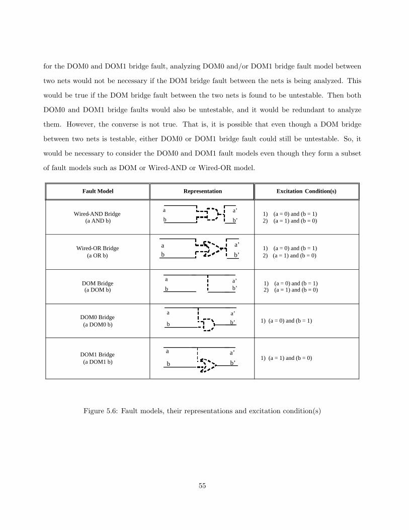
for the DOM0 and DOM1 bridge fault, analyzing DOM0 and/or DOM1 bridge fault model between

two nets would not be necessary if the DOM bridge fault between the nets is being analyzed. This

would be true if the DOM bridge fault between the two nets is found to be untestable. Then both

DOM0 and DOM1 bridge faults would also be untestable, and it would be redundant to analyze

them. However, the converse is not true. That is, it is possible that even though a DOM bridge

between two nets is testable, either DOM0 or DOM1 bridge fault could still be untestable. So, it

would be necessary to consider the DOM0 and DOM1 fault models even though they form a subset

of fault models such as DOM or Wired-AND or Wired-OR model.

Fault Model Representation Excitation Condition(s)

Wired - AND Bridge (a AND b)

a

b

a’

b’

1) (a = 0) and (b = 1) 2) (a = 1) and (b = 0)

Wired - OR Bridge (a OR b)

a b

a’

b’

1) (a = 0) and (b = 1) 2) (a = 1) and (b = 0)

DOM Bridge (a DOM b)

a

b a’ b’

1) (a = 0) and (b = 1) 2) (a = 1) and (b = 0)

DOM0 Bridge (a DOM0 b)

a

b b’

a’

1) (a = 0) and (b = 1)

DOM1 Bridge (a DOM1 b)

a

b

a’

b’

1) (a = 1) and (b = 0)

Figure 5.6: Fault models, their representations and excitation condition(s)

55

5.4 Algorithm

The following definition of an observation point is necessary to understand before we can discuss

the algorithm:

Definition 1: (Observation point)

An observation point for a fault is defined as the nearest fanout stem, a primary output or a latch

element, in the fanout cone of the fault site.

Also, our analysis is based on the ILA (iterative logic array, of fixed length K) representation

of a sequential circuit, where the latch elements of the lowest time frame (i.e.frame −K/2) of the

ILA are fully controllable, and the latch elements in the right most time frame (i.e. frame K/2) are

fully observable. Figure 5.7 outlines the overall algorithm.

Let us look at the algorithm in detail:

1. Symbolic simulation and absorption of stuck-at information: As discussed earlier, we perform

a sequential symbolic simulation using 11 symbols, to identify controllability characteristics of

nets in the circuit. At the beginning of the simulation, we associate the primary inputs (PIs) and

the controllable latch elements with the symbol ControllableToAny, and the other sequential

(latch) elements with the symbol UncontrollableToAny, and propagate these symbols across

the circuit. We use the table look-up scheme described earlier, until the circuit stabilizes to

steady state w.r.t. symbolic values.

We absorb a fault list which lists all untestable stuck at faults in the circuit, and screen out

certain bridge faults before starting the per-fault analysis. For example, if the fault bstuck−at0

is untestable, then the bridging fault aDOM0b between nets a and b would also be untestable,

and can be dropped from the original bridge fault list. Our tool that identifies untestable stuck-

at faults is based on symbolic simulation and Boolean satisfiability analysis, but we would not

discuss the details of that tool in this discussion.

56

a) Perform Symbolic Simulation to obtain information

about constants in the circuit.

Also, absorb the untestable stuck-at information to

screen out some bridging faults.

b) For the remaining fault (per-fault analysis):

b.1) Find the necessary condition(s) to excite the fault,

and to propagate the fault effect to an Observation Point.

b.2) Backward imply/justify these set of conditions

b.3) If no conflict exists, forward imply with the logic

values set in the circuit. If a conflict exists in either

backward or forward implications, the bridge fault is untestable.

b.4) Perform observability analysis to determine if the

fault effect can be propagated to a PO or to a latch

boundary in the last time frame of the K-frame unrolled circuit.

Figure 5.7: Algorithm for untestable bridge fault identification

2. Per-Fault Analysis: After filtering the initial fault list, we perform the following analysis on

each fault in the reduced list:

(a) Identification of conditions necessary for fault detection: Depending upon the fault type,

we identify the fault site and the condition(s) for fault excitation (as previously shown

in Figure 5.6). For example, if a aDOM0b bridge exists between nets a and b, then the

fault excitation condition would be (a = 0) and (b = 1), and the fault site would be net

b, because a fault effect of 0/1 (good machine value / faulty machine value) appears on

this net. Then, we identify the conditions necessary to propagate the fault effect to an

observation point. This basically means that we identify the non-controlling values on

57

each gate in the off-path from the fault site to the observation point. These conditions

must be met if the fault has to be testable.

(b) Backward implications:A backward implication routine is then invoked on the necessary

set of conditions. We could have separately implied each necessary condition and added

the individual implication lists to obtain the composite implication list corresponding to

the set of necessary conditions. This is exactly what would have been done if implications

corresponding to each gate were computed as a pre-processing step. However, we compute

the implications associated with the entire set of necessary conditions in one go, because

this technique helps in learning more implications. The backward implication process

begins at the fault injection frame, and goes on till the lowest time frame in the ILA

expansion is reached (i.e. −K/2, in an ILA representation of K frames) or till no more

implications can be learnt.

(c) Forward Implications: If no conflict is encountered in the backward implication process,

then a forward implication process is invoked on the already learnt implication set. This

implication process begins at the lowest level of the ILA expansion, and continues till the

last frame of the ILA is reached (i.e. begins at −K/2, or the lowest frame that has a valid

implication associated with it, and continues till frame K/2) or till no more implications

can be learnt.

(d) Observability Analysis: If no conflict occurs during either the backward implication process

or during the forward implication process, then an observability analysis is carried out to

determine if the fault effect can be observed or not. This observability analysis marks the

last step of untestability analysis for a fault, and the motivation behind the observability

analysis is to check if the excitation conditions for the fault block the fault effect from

propagating to the primary output(s) or not. The way we implement this observability

analysis is through multiple ID propagation. This is explained below: We associate an ID

with the fault site, (say X), and propagate it through the circuit. We also keep a track

of the polarity of this ID, and identify the inverted value of this ID as X. This is done to

identify masking of fault effects (For example, if an id of X and X appear at the input of

58

an AND gate, the fault effect would get killed due to the opposite polarities of the fault

IDs). Since most of the industrial designs contain tri-state devices, and buses, we use

another ID, which is a generic ID, and we call it IDG. The motivation of using IDG can

be understood through Figure 5.8.

0

1

X

Z/0

Z/1

Figure 5.8: Use of Generic ID : IDG

Let’s assume that fault ID X (lets assume X represents a faulty state of 0/1) appears at

the select line of a tri-state device, as shown in Figure 5.8, with an active high enable.

The faulty machine value at the output of the gate would be the value applied at the

input of the gate, but the good machine value will be Z, i.e. high impedance state. A

fault effect of Z/0 or Z/1 cannot be directly associated with either X or X (because X

and X are of the form 0/1 or 1/0). Thus, this fault effect is represented by a new ID, i.e.

IDG. Thus, if any of these IDs, i.e. X, X R or IDG propagate to either a PO or to the

latch boundary in the last time frame of the ILA expansion, then the fault is not declared

untestable. However, if none of these IDs can propagate to a completely observable point,

then the bridge is marked as untestable.

5.5 Results

The proposed algorithm was implemented in C++ and experiments were conducted on ISCAS89

and some industrial circuits on a 500 MHz, HP workstation. The results are reported in Table 5.1.

Column 1 in Table 5.1 shows the ISCAS ’89 circuits, and the industrial circuits (C1, C2, C3) for

59

Table 5.1: Results Obtained for 16000 randomly generated bridges

Circuit ATPG Red. Suntest Suntest Time (sec) Time (sec)

(bk = 1000) ∗K = 2 K = 0 K = 2 K = 0

s5378 261 552 176 361 40

(187/365) (176/0)

s9234 965 5585 5568 356 47

(679/4906) (676/4902)

s13207 1595 13163 13160 318 31

(1485/11711) (1485/11708)

s15850 496 1190 1183 804 95

(230/960) (228/955)

s35932 1382 945 927 979 534

(915/30) (897/30)

s38417 535 428 418 2139 100

(115/311) (111/307)

s38584 1113 868 861 3085 846

(714/154) (711/150)

C1 154 39 39 63 23

(39/0) (39/0)

C2 43 27 27 90 63

(27/0) (27/0)

C3 76 21 21 97 14

(21/0) (21/0)

∗K = ±Number of time frames in which the sequential circuit is unrolled

60

which the tool was evaluated. Column 2 shows the number of faults our bridge fault ATPG engine

identified as untestable, with the backtrack limit set to 1000. Column 3 shows the number of faults

identified as untestable using the new implications-based tool, with the time frame expansion of the

circuit being from -2 to 2. The numbers in the parenthesis in this column show two values. The first

value is the number of faults identified as untestable both by the new tool and by ATPG, and the

second value in bold identifies the number of faults that our tool identified as untestable, for which

ATPG aborted after 1000 backtracks. For example, for circuit s5378, ATPG identified 261 faults as

untestable. With the implications based approach, we identified 552 faults as untestable. Out of

these 552 faults, 187 faults were identified as untestable by both ATPG and the implications based

tool, while the rest 365 faults identified as untestable, were the faults on which ATPG aborted. So,

the gain here is w.r.t the 365 faults which our new tool could identify as untestable, while for which

ATPG could not generate a pattern. Column 4 shows the number of faults identified as untestable by

the new tool, using K = 0, i.e. by unrolling the sequential circuit in just one time frame (effectively

combination analysis). Finally, columns 5 and 6 show the time taken by the implications based tool

to analyze all faults for an ILA size of 5 (K = 2) and ILA size of 1 (K = 0) respectively.

Table 5.2 shows the time spent by ATPG to analyze the faults identified as untestable using

the implications based algorithm. Column 1 in Table 5.2 shows the circuit name, and the 2nd

column shows the time spent by ATPG only on the faults which were identified as untestable using

the implications based tool (Sunt for K = 2). For example, for s15850, the ATPG engine took 953

seconds to analyze the 1190 faults identified as untestable by our tool for K = 2. It was observed

that the number of untestable faults identified with K = 0 (combinational analysis) is almost the

same as the number of faults identified by expanding the ILA to a length of 5 frames for most of

the circuits. Thus, it can be seen that even in a combinational framework, our tool can quickly

identify more untestable faults than the ATPG tool can capture. It was also seen that although

our implications based approach for identifying untestable bridges worked out better than ATPG for

ISCAS circuits, it identified only a subset of untestable faults identified by the ATPG engine for the

industrial circuits. This is primarily due to the fact that the bus structures present more commonly in

industrial designs limit the strength of implications, and hence limit the untestable fault identification

61

Table 5.2: Time taken for ATPG to analyze Suntest

Circuit TimeATPG

(sec)

s5378 58

s9234 592

s13207 14380

s15850 953

s35932 60

s38417 86

s38584 405

C1 10

C2 13

C3 8

capability. Nevertheless, our tool provides a novel technique to quickly identify non-trivial untestable

bridging faults, thereby reducing the size of the bridging fault list to be analyzed.

62

Chapter 6

Conclusions and Future Direction

In this thesis, we presented:

1. A theorem that can be used to identify more untestable stuck-at faults in sequential circuits

(using fault independent, single line conflict approach) than could be identified by the tra-

ditional methods based on the principle of single line conflicts or by fault oriented methods

such as the single fault theorem(with the same ILA expansion). We demonstrated through our

results that by using the proposed theorem, we could identify more untestable stuck-at faults

with an ILA of size 3 than could be identified by the traditional methods even by incrementing

the ILA size to upto 11. We implemented a powerful implication engine as the basic framework

of this untestable fault identification engine. We boosted the execution speed of this impli-

cation engine by doing a selective extended backward implication without letting any loss in

the performance of the tool in terms of the number of untestable faults identified. We further

propose that fault oriented approaches can benefit from the proposed theorem to identify more

untestable faults (at a higher expense in terms of execution time) than the fault independent

approaches can.

2. An approach to combine the implications of two nets in the circuit, and use that information to

identify more untestable faults than can be identified by single line conflict. If the circuit has

n gates, then the complexity associated with the combination of all pairs of gates in the circuit

can be of the order of n2. Therefore, we presented a technique to intelligently combine nets

63

in the circuit to form pairs, so that the complexity of this technique can be reduced without

letting the number of untestable faults identified by this technique fall by a lot.

3. A technique to identify untestable bridging faults based on implications and symbolic simula-

tion. We performed an 11-symbol simulation as a pre-processing step to identify uncontrollable

nets in the design. We then used the information provided by the untestable stuck-at faults

to filter out some untestable bridges early in the analysis process. We then used implications

associated with the necessary conditions required to detect the bridging fault, and the infor-

mation provided by the symbolic simulator to identify untestable bridges. We validated and

compared our results with an internal ATPG tool for bridging faults and found that we could

quickly identify a lot of non-trivial untestable bridges for which the ATPG tool aborted for

large sequential circuits. Thus, the performance of the ATPG tool in terms of execution time

can be increased by complimenting it with our tool. However, we also found that the power

of implications is greatly hit by more commonly present bus-structures in industrial designs.

However, we believe that by incorporating extended backward implications (which are not cur-

rently implemented due to reasons related to execution speed) into the implication engine, we

can achieve a higher success w.r.t. identifying untestable bridges in large industrial designs

too.

6.1 Future Direction

In our method used to identify extra untestable faults using multiple node implications, we ex-

plored just one characteristic of the circuit that can lead to redundancy, i.e. reconvergent stems.

However, we believe that there could be some other characteristics that can be further explored to

combine nets in pairs that can help increase the number of untestable faults identified. Also, it was

found that although our technique helps identify more untestable faults, the overall cost in terms of

execution time paid for this increase is quite large. So, the number of gate pairs should be trimmed

further if possible so as to boost the speed of the entire algorithm.

In the work presented by Hsiao [10], local impossible combinations of nets were explored. When

64

an impossible combination of node values was identified, faults that required this impossible combi-

nation as a necessary condition for their detection were enumerated. The underlying principle here

is that since this combination can never occur, faults that require this combination of node values

either for their excitation or their propagation would be untestable. We believe that in addition to

these local conflicting scenarios, there could be some global impossible value combinations, which

could help in identifying more untestable faults. However, the important thing to note is that such

global combinations should be non-trivial, and the method to identify these conflicting values should

not be too expensive in terms of time.

None of the ideas mentioned above have been explored yet, and hold good potential for research.

65

Bibliography

[1] M. A. Iyer and M. Abramovici, “FIRE: a fault independent combinational redundancy algo-

rithm”, IEEE Trans. VLSI, June 1996, pp. 295-301.

[2] V. D. Agrawal and S. T. Chakradhar, “Combinational ATPG theorems for identifying untestable

faults in sequential circuits”, IEEE Trans. Computer-Aided Design, vol. 14, no. 9, Sept. 1995,

pp. 1155-1160.

[3] S. M. Reddy, Irith Pomeranz, X. Lim and Nadir Z. Basturkmen, “New procedures for iden-

tifying Undetectable and Redundant Faults in Synchronous Sequential Circuits”, VLSI Test

Symposium, 1999. Proceedings. 17th IEEE, 1999, Page(s): 275-281.

[4] M.A. Iyer, D.E. Long, Abramovici, “Identifying sequential redundancies without search”, Pro-

ceedings Design Automation Conference, 1996, pp. 457-462.

[5] J. Rajski and H. Cox, “A method to calculate necessary assignments in ATPG”, Proceedings

Int’l. Test Conference 1990, pp. 25-34.

[6] W. Kunz and D. K. Pradhan, “Recursive Learning: A new implication technique for efficient

solutions to CAD problems-test, verification, and optimization”, IEEE Trans. On CAD, Sept

1994, pp. 1149-1158.

[7] J. Zhao, M. Rudnik, J. Patel, “Static Logic Implication with application to fast redundancy

identification”,Proceedings VLSI Test Symposium, 1997, pp. 288-293.

[8] K. Gulrajani and M.S. Hsiao, “Multi-Node Static Logic Implications for Redundancy Identifi-

cation”, Proceedings Design Automation and Test in Europe Conference, 2000, pp. 729-733.

66

[9] J. Zhao, J. A. Newquist and J. Patel, “A graph traversal based framework for sequential logic

implication with an application to c-cycle redundancy identification”, Proceedings VLSI Design

Conference, 2001, pp. 163-169.

[10] M. S. Hsiao, “Maximizing Impossibilities for Untestable Fault Identification”, Proceedings IEEE

Design, Automation and Test in Europe Conf., March 2002, pp. 949-953.

[11] D. E. Long, M. A. Iyer, M. Abramovici, “FILL and FUNI: Algorithms to identify illegal states

and sequentially untestable faults”, ACM Transactions on Design Automation of Electronic

Systems, pp 631-657.

[12] Hsing - Chung Liang, C. Len Lee, Jwu E. Chen, “Identifying untestable faults in sequential

circuits”. IEEE Design and Test of Computers, Fall 1995, Pages 14-23.

[13] S. T. Zachariah, S. Chakravarty, C. D. Roth. “A novel algorithm to extract two-node bridges”,

Proceedings Design Automation Conference, 2000. pages 790-793.

[14] S.T. Zachariah, S. Chakravarty. “A novel algorithm for multi-node bridge analysis of large VLSI

circuits”, Proceedings VLSI Design, 2001, pages 333-338.

[15] S.D. Millman, E.J. McCluskey, and J.K. Acken, “Diagnosing CMOS bridging faults with stuck-

at fault dictionaries”, Proceedings Int’l. Test Conference, 1990, pages 860-870.

[16] S. D. Millman, Sir J.P. Garvey. “An accurate bridging fault test pattern generator”, Proceedings

Int’l. Test Conference ,1991 , pages 411-417.

[17] P.C. Maxwell and R.C. Aitken. “Biased voting: A method for simulating CMOS bridging faults

in the presence of variable gate logic thresholds”, Proceedings Int’l. Test Conference, 1993,

pages 63-72.

[18] M. Abramovici, M.A. Breuer and A.D. Friedman, “Digital Systems Testing and Testable De-

sign”, Computer Science Press, 1990.

67

Vita

Manan Syal was born in Mehsana, a small town in Gujarat, India. He did his schooling partly

from Dehradun and partly from Mumbai, India. He joined K.J. Somaiya College of Engineering

under the Mumbai university in 1996, to obtain technical education in the area of electronics. After

graduating with a bachelor’s degree in Electronics Engineering in July 2000, he joined Virginia

Polytechnic Institute and State University in August 2000 for a Masters degree in the Bradley

Department of Electrical and Computer Engineering. He joined Dr. Michael Hsiao and his research

group in August 2001 and has since then been involved in research related to hardware testing.

Manan’s hobbies include sketching, hiking, music and generally having fun with his friends. His

technical interests include VLSI testing, verification and VLSI design. His long term goals are to

contribute to the scientific community in the areas of hardware testing and verification during and

after his PhD.

68