Lthvt. feppr~s RWWA ew - VTechWorks

A Simple Finite Element For The Dynamic Analysis of Rotating Composite Beams

by

Vikas B. Dhar

Thesis submitted to the Faculty of the

Virginia Polytechnic Institute and State University

in partial fulfillment of the requirements for the degree of

Master of Science

in

Aerospace and Ocean Engineering

APPROVED:

Lthvt. feppr~s RWWA ew Rakesh K. Kapani4, Chairman Raphael ‘MHaftka

= Eric R. Johnson William H. Mason

May, 1990

Blacksburg, Virginia

LD S655 VESS 1990 D437 ds

A Simple Finite Element For The Dynamic Analysis of Rotating Composite Beams

by

Vikas B. Dhar

Rakesh K. Kapania, Chairman

Aerospace and Ocean Engineering

(ABSTRACT)

An attempt is made to understand the phenomenon of aeroelasticity as applied

to the helicopter rotors, specifically laminated composite rotor blades. Realizing

the immense complexity of the problem, a beginning has been made by

developing a structural model for a rotating composite beam. Present work has

three objectives; 1) To carry out an extensive survey of research related to the

aeroelastic analysis of rotor blades, 2) To expand an existing finite element model

by introducing new degrees of freedom and validate the changes, 3) and, finally

using this model to carry out a linear static and dynamic analysis for a rotating

composite beam. It was found that the rotation and fiber orientations have a

pronounced effect on the static deflections and the natural frequencies of

vibration of the laminated beam.

Acknowledgements

My thanks are due to Dr. Rakesh K. Kapania for his constant help and advice,

and Drs. Raphael T. Haftka, Eric R. Johnson, and William H. Mason for serving

on my committee. I would also like to thank Dr. J. A. Schetz, Head of the

Department, for providing me with timely financial assistance.

Acknowledgements iti

Table of Contents

Nomenclature ....... csc ccc c ccc cere e cece creer sere cece rears er eeeeesesseens 1

Introduction 2.2... cc ccc ccc ce ccc cere cree nee e cece rece cerca reer eer esseseeene 6

Literature Survey 2... ccc cc ccc cee cere meee ee eee eee e eee eee neeeeeess 17

Introduction 2.0... ccc cc ee ee eee eee ete eee te eee eee ete e eee ees 17

Structural Modeling ... 2... ccc ccc et cect ete eee ete e eet eeeeeens 18

RevieWS 2... ccc cece cee eee tne e eee eee eee este nen eeneeeenees 18

Isotropic Blades 2... eee ct eee eee eee eee eee tee eee eens 20

Composite Rotor Blades 2.0... .... ccc ccc ce eee ence e eee eee eees 26

Aerodynamic modeling ....... ccc cc ccc ccc ee ce eet ete teen ee eee ee eenas 32

Classical Unsteady Aerodynamic Theories. .........0 cc eee cece cee cece eet eeees 34

Three Dimensional Vortex Theories ......... cc cece cece ec ee eee eee eee eee 37

Dynamic Inflow Theory ......... 0. cc cece cece eee eee eee eee eee tence eens 39

Models ..... 2... ccc cree cern reece ree c cere reece care sere cere reece see eeeee 41

Structural Model 2.0... cc ee eee ee ee ee eee eee te eee eee eens 41

Table of Contents iv

Incremental Stiffness Matrix .. 0.0... ce ee cee ee ee eee eee eee eee eee 47

Static Deflection and Free Vibration Analysis ......... 0... cece eee eee ee eee eens 50

Aerodynamic Model 2.2.1... cc cc ee eee eee ee ee eee eee nee eee eee 51

Solution for Aeroelastic results. 2... 0... ccc ee wee ee tee eee eee tee cease 52

Results 2... ccc ccc ccc cee cree re cee eee ee eee eee ee tee eee eee e nets nee eees 54

Validation ... ccc cc cee ee ee tee ee ee eee ne eee ee tee eee eee enes 56

Static deflections .. 0... ccc ccc ce cc ee cee tte et ee ee eee eee et eee eee ee eee 56

Free Vibrations 2.0... . 0... ccc ee cee ee eee tee eee eee ee ete e ee eee eees 57

Aeroelastic results 2.0... ccc ce ee cee ee tee eee ete ee eect eee ee eee tees 59

Results from the rotating beam. 2... ec eect eee eee te ee eee eee ee teee 59

Static deflections. 2.2.0.0... ccc cc ec ce ce ee ee ee eee eee eee ee eee eee eee eae 60

Free Vibration. 2... 0... ccc ee cc ce ee eee eee eee ee ee ee eee eee ee enee 60

Conclusions and Recommendations for Future Work .........cccccccccccsccvecececs 62

References 2... cc ccc ccc cc ccm ec cece we eter eee cece ene eect eee e tect es eees 64

Figures and Tables 2.0... . cc cece ccc ccc cer werner cece eee eee e eres esses eeees 15

Appendix A. The Incremental Stiffmess Matrix ....... ccc cccceccccceccercescccees 98

Appendix B. The Data File 2.0... . ccc cece cece cece cence cere anew senses seenes 101

Vita Coc ccc ce ccc ce ee eee eect eee ete t ee eaten tee tee cess ee seeee 142

Table of Contents v

List of Illustrations

Figure

Figure

Figure

Figure

Figure

Figure

Figure

Figure

Figure

Figure

Figure

Figure

Figure

Figure

Figure

Figure

Figure

Figure

1. a)A typical Helicopter configuration b) defining precone and droop ......... 80

2. Various hub configurations of rotor blades, Reference[7] .............05- 81

3. Typical Helicopter rotor configuration ............. vceeueueeucueeues 82

4. Block diagram of inflow dynamics ........... ccc eee c eect eee e neces 83

5. Built-up blade model. 2.2... kc eect eee eee eens 84

6. Element degrees of freedom ......... cece ccc eee eee ee eee teen eens 85

7. Strain-Displacement Matrix ............e00. cee eee ee eee ee ete 86

8. Configuration of a rotating beam. .. 1.1... cee eee eee eee tes 87

9. Distribution of deflections due to bending and shear deformations and twisting angle fora l6 ply [45,/ —45,], underatip load 2... 0... ccc eee ce eee eee 88

10. Box Beam Geometry Ref. [14] 2... .. ccc ce cece eee eee eens 89

11. Box Beam Tip Deflection Under a Tip Load... cece cee ccc eens 90

12. Critical Speed of an Unswept Graphite/Epoxy Plate,(@,/0), ...........45. 91

13. Flutter and Divergence Speeds of an Unswept Box Beam ...............-.. 92

14. Tip deflection vs 6 for a rotating (@,/0), plate. .. 0... . cc eee ce eens 93

15. Variation of first natural frequencies of vibration with angular velocity for an isotropic beam, R = 0... ec eee eee ee eee eee eens 94

16. Variation of first natural frequencies of vibration with angular velocity for isotropic beam with different values of Row... cee eee ee eet eens 95

17. Variation of first natural frequencies of vibration with angular velocity for the Graphite/Epoxy plate R = 0. 2... cece ec eee eee teen eee 96

18. Variation of first natural frequencies of vibration with angular velocity for the Box-Beam with different values of R 1.1... ccc ee ee ee ee ee tees 97

List of Illustrations vi

List of Tables

Table 1. Maximum deflection w, in pe due to shear deformation only ............. 76

Table 2. Natural frequencies for the Aluminium plate ........... 0c cee eee eee eens 77

Table 3. Natural Frequencies of a 30 Degrees Off-Axis Graphite/Epoxy Cantilever Beam . 78

Table 4. Natural frequencies of a [ 45, /0,], Boron/Epoxy plate .............e ee eee 79

List of Tables Vii

Nomenclature

Ay 5 inf =1,...56

Ay

[A]

b

b,

By, inf =1,..056

c

C(k,)

Nomenclature

non-dimensional offset between semichord and origin

nondimensional offset between the aerodynamic center and the mid chord

section lift curve slope

complex element aerodynamic matrix

elemental area

extensional stiffness coefficients

transverse shear stiffness

assembled aerodynamic matrix

beam chord

reference airfoil semichord

bending-extension stiffness coefficients

chord of the cross - section

Theodorsen’s circulation function

H, ,i=1,...,5

J

Jn

k

k,

[k]

K

[K]

[KG1]

[KG2]

[KG3]

Nomenclature

lift curve slope

bending stiffness coefficients

beam force-strain matrix

cover skins force-strain matrix

distance between aerodynamic center and the elastic axis of the cross-section

undeformed blade reference axes

deformed blade reference axes

Stringers’ moduli

element nodal load vector

assembled nodal load vector

centrifugal force at x’

damping coefficient

Gaussian quadrature weights

mass polar moment of inertia

Bessel function of the first kind

reference reduced frequency

reduced frequency

element stiffness matrix

Timoshenko’s shear factor

assembled stiffness matrix

constant part of the incremental stiffness matrix

linear part of the incremental stiffness matrix

quadratic part of the incremental stiffness matrix

l

L

Ly Ly Ly, Ly:

[m]

M

M,, M., My, M,

Mr, M:, M, M,,

(M]

n

N,,i=1,...54

Ney Nyy Ney Nez

N,, Ni Noy N-

{N}

p

q

{q}

[2]

r

R

R

[S]

T

Nomenclature

element length

aerodynamic lift

lift components

element mass matrix

aerodynamic moment

aerodynamic moment components

plate resultant moments

assembled mass matrix

total number of skin layers

Hermitian interpolation polynomials

plate resultant forces

aerodynamic displacements interpolation vectors

resultant force vector

number of elements covered

total number of elements in the analysis

nodal displacement vector

reduced transormed local stiffness matrix

offset between center of gravity and origin

radius of the hub

radius of the hub non - dimensionalized w.r.t. the element length.

transformation matrix from undeformed to deformed state

element Kinetic energy

YA, YB, YD ,i=1,...,6

B

?

5W

x9 Eps Vey

Exy Eyy Vays Vz

{e}

1%}

Nomenclature

axial displacement

element strain energy

element strain energy due to the centrifugal force

lateral deflection due to bending

flow speed over the blade

transverse deflection

wake spacing function

transverse deflection due to bending

transverse deflection due to shear

element dimensional coordinate system

element dimensional coordinate axis along the length of the element.

Gaussian quadrature abscissas

global coordinate system

Bessel function of the second kind

stiffness coefficients pertaining to the lateral deflection

in-plane shear angle

beam material density

Aerodynamic forces virtual work

reference surface in-plane strains

local strains

active strain vector

reference surface strains and curvatures vector

6,

6,

Ky Ky, Ky, K

p

pA

Nomenclature

xy

non-dimensional elemental coordinate along the length

non-dimensional chordwise coordinate

transverse bending slope

transverse shear slope

curvatures

non-dimensional spanwise coordinate

air density

element mass per unit length

twist angle

twist angle component due to the geometric transformation of the transverse shear slope @,

torsion variable

beam oscillation frequency

angular velocity of the rotating beam

Introduction

Aeroelasticity is a branch of science which is concerned with the motion of

deformable bodies through fluids. It is often also defined as, a science which

studies the mutual interaction between aerodynamic, inertial and elastic forces

and its influence on airplane design and performance. One more and a rather

graphic way of defining it could be “as an interface between solid and fluid

mechanics, with dynamics serving as the adhesive ” [ 1 }. Regardless of the choice

of simile, however, engineers in the field of aircraft and missiles are well aware

of its existence and influence on the success of their designs.

Aeroelastic problems would not exist if airplane structures were perfectly rigid.

Modern airplane structures are flexible, and this flexibility is fundamentally

responsible for various aeroelastic phenomena. On its own structural flexibility

may not be objectionable. But when the deformations in a flexible structure

Introduction 6

induce additional aerodynamic forces, which in turn lead to higher deformations

and so on, they are singled out as the culprit. Problems in the realm of

aeroelasticity are diverse and they are a fast multiplying species. Their

classification; however, quite ingeniously done by Collar [ 2 ] back in 1946, still

remains widely accepted. The triangle of forces, with aerodynamic, elastic and

inertia forces at the three vertices show how these forces interact to pose a wide

variety of problems for an aeroelastician. Duncan [ 3 J, in 1968, suggested

another way of classifying the aeroelastic problems. They may be classified in the

first place as oscillatory or non-oscillatory, further depending on the role

flexibility plays in the phenomena.

Group A Phenomena in which structural flexibility plays an important

part.

A.1 Non-oscillatory phenomena

A.2 Oscillatory phenomena

Group B Phenomena in which structural flexibility does not play an

essential part.

B.1 Non-oscillatory phenomena.

B.2 Oscillatory phenomena.

Introduction ”

The phenomena of Group A would not occur if the structure could be made rigid.

Those in Group B are significantly influenced by structural flexibility but could

still occur in its absence. The content of various categories are as follows;

A.l Structural divergence of surfaces

Reversal of control.

A.2. Flutter

B.1 Non-oscillatory behaviour of the aircraft as a whole ( in relation to

stability, control and response )

B.2 Snaking and longitudinal snaking

Oscillatory behavoiur of the aircraft as a whole.

Buffeting.

The growth of aeroelasticity in its early years was not in any way very general

or abstract. It had been developed with the immediate aim of application to

aeronautics. Hence it grew under the stress imposed by the urgent practical

demands and new techniques had to be developed in an ad hoc fashion. In fact

the problem of aeroelasticity did not attain the prominent role it plays now until

the early stages of WW-II. Prior to that time, airplane speeds were relatively low

Introduction 8

and the load requirements placed on the aircraft structures by design criteria

specifications produced a structure sufficiently rigid to preclude any aeroelastic

phenomena. As speeds increased, however, with little or no increase in load

requirements, and in absence of a rational stiffness criteria for design, aircraft

designers encountered a wide variety of problems in aeroelasticity, the ones

classified above.

Although aeroelastic problems have occupied their prominent position for a

relatively short period, they have had some influence on airplane design since the

beginning of the powered flight. Perhaps the first designer to be effected was

Professor Samuel P. Langley of the Smithsonian Institution. It seems likely that

the unfortunate wing failure which wrecked Langley’s machine on the Potomac

river houseboat in 1903, could be described as a wing torsional divergence.

Perhaps the success of the Wright biplane and the failure of Langley’s monoplane

was the original reason for the dominance of the biplanes till the mid-thirties. The

most widespread early aeroelastic problem in the days when military aircraft were

almost exclusively biplanes was the tail flutter problem. One of the first

documented cases of the flutter occured on the horizontal tail of the twin-engined

Handley Page 0/400 bomber in the beginning of the WW-I. A second epidemic

of tail flutter was experienced by DH-9 airplanes in 1917, and a number of lives

were lost before it could be cured. The Fokker D-8 played havoc on the German

Air Corps in WW-I. Since the aircraft was high-tech for its time, only the cream

of the airforce got to handle it. Unfortunately the aircraft had a number of

crashes and many ace pilots were lost. The cause was collapse of wing in torsion

Introduction 9

due to very high loads at the tips under the strains of combat manoevers. After

the war the D-8 also demonstrated a non-destructive kind of bending-aileron

flutter.

The period of developement of the cantilever monoplane seems to have been the

period in which serious research in aeroelasticity commenced. Today the subject

is quite well developed and boasts of contributions to fields other than

aeronautics. Aerothermoelasticity, for example, deals with the effect of

temperature, Aeromagnetoelasticity similarly studies the effect of the strong

magnetic field, like that of earth, on the airplane design. Another of the often

repeated terms is Aeroservoelasticity, which takes into account the effect of

dynamics of guidance and control on aeroelasticity.

Although the technological cutting edge of the field of aeroelasticity has centered

in the past on the aeronautical applications, applications are found at an

increasing rate in Civil Engineering; e.g. flows about bridges and tall buildings;

Mechanical Engineering; e.g. flows around turbomachinery blades and fluid flows

in flexible pipes; Nuclear Engineering; e.g. flows about fuel elements and the heat

exchanger vanes. It may well be that such applications will increase in both

absolute and relative number as technology in these areas demands light weight

structures under severe flow conditions.

Coming back to the aeronautical applications we have overlooked an important

group of flight vehicles influenced rather strongly by the aeroelastic phenomena,

Introduction 10

namely those of Rotary-Wing airplanes or Helicopters, as they are popularly

called ( Autogyros, have become history after an unimpressive Start).

Notwithstanding the developement of the conventional airplane, we have been

aware that helicopters are the only means to achieve complete mastery of the air;

namely, the ability to stay aloft without maintaining forward speed (what is

technically hovering ) and to ascend and land vertically in restricted areas. A

basic introduction to aerodynamics and mechanics of helicopters may be found

in References [ 4] and[ 5 J.

It will be in order to mention the V/STOL aircraft configurations which make use

of rotors or propellers for the necessary lift or thrust. Even these otherwise

conventional aircrafts often have a design criterion based on rotor or propeller

Stability.

Dynamic stability and response problems associated with rotary-wing aircrafts

represent some of the most complex problems in the area of aeroelasticity. There

are two basic sources of this complexity. “ One is the unusual flexibility of the

prop-rotor blades (even in the case of so-called rigid rotors), and the other is the

complexity due to rotation. Flexibility manifests itself both by adding degrees of

freedom which can be important and by allowing initial deflections to be large

enough to add coupling terms between degrees of freedom. Rotation, of course,

leads to 1) much more complicated inertia forces (e.g., centrifugal, Coriolis,

gyroscopic) which must always be regarded as potential sources of stiffness or

coupling between the degrees of freedom, and 2) an aerodynamic situation of

Introduction 11

exquisite intractability ” [ 6 ]. The stability problems in helicopters is dealt in two

steps, first by considering an isolated blade and a fixed hub, and secondly by

carrying out a coupled aeroelastic analysis of rotor and fuselage by assuming a

movable hub. Types of motion exhibited by the blade and fuselage of a typical

helicopter are shown in Figure 1.

Due to the complicated nature of the aeroelastic problems, rotary- wing

aeroelasticity had been considerably less developed than its fixed-wing

counterpart. This field has seen intense activity in the last three decades. Still

since the classical books in aeroelasticity date back to 50s or 60s, one does not

even find a mention of this field of comparable importance.

Over the years a number of configurations of the rotor blades have been

developed, each with a specific purpose in mind. The ones in extensive use can

be divided into four types , as shown in Figure 2 [ 7 ], ; These are (i )

semi-articulated or see-saw, ( il ) articulated, ( ili ) hingeless and lastly ( iv )

bearingless rotors. The see-saw rotor ( Bell ) is typically a two-bladed rotor with

the blades connected together and attached to the shaft by a pin which allows the

two-blade assembly to rotate such that tips of the blades may freely move up and

down with respect to the plane of rotation (flapping motion). In the fully

articulated rotor, each blade is individually attached to the hub through two

perpendicular hinges allowing rigid motion of the blade in the two directions, out

of the plane of rotation (flapping) and in the plane of rotation ( lead-lag ) as

typified by Sikorsky, Boeing-Vertol and Hughes helicopters.The third type is the

Introduction 12

hingeless rotor in which the rotor blade is a cantilever beam. Being a long thin

member, elastic deformations of the hingeless blade are significant in the analysis

of the dynamics of the vehicle. Both hingeless and bearingless rotors were built

with an eye on mechanical simplicity and increased maintainability. A bearingless

design eliminates the hinges and the pitch bearing found in an articulated rotor.

Some bearingless designs employ lag dampers. The bearingless blade has an

elastic flexure consisting of flexbeams and a torque tube to facilitate pitch

changes.

Other recent developements in the rotor configuration are the Tilt rotor [ 8,9 ],

ABC rotor [ 10,11 ] and the circulation rotor [ 12,13 ].

Present day rotor blades are often made up of composite materials, which have

found increasing use in the field of structural design. Composites unlike the

metallic counterpart have direction dependent properties. And the fact that they

have very high strength to weight or stiffness to weight ratio is of essence. A wise

manipulation of these properties can lead to cheaper and much lighter designs.

For the laminated composites, the stacking sequence of the plies is of primary

importance, which divide them into symmetric and asymmetric categories. The

elastic couplings exhibited by both these categories are often used in, what is now

popularly termed as Aeroelastic tailoring. As the name suggests, fiber composites

are cut and pasted in a particular fashion so as to yield desirable results. This has

been possible owing to highly directional behaviour of the these materials. Some

of these couplings in the elastic stiffness matrix are,

Introduction 13

e Bending-Extension

e Shear-Extension

e Twist-Bending couplings.

The first of these is exhibited only by the unsymmetrically laminated

plates/beams, which basically means that the in-plane and the out-of-plane

problems are coupled. Much more, in terms of strength, weight and life is

expected of today’s structures, which has what led to the increasing research in

the field of composite structures which provide much more flexibility than their

isotropic counterpart.

Castel and Kapania [ 14 ] have presented a one dimensional model of a composite

laminated beam amenable to linear aeroelastic analysis. They developed a 24

degree of freedom finite element which is capable of analysing a beam/plate of

arbitrary cross-section, planform, taper and sweep. The special features of the

analysis are the inclusion of shear deformation, warping correction factor, and its

capability to study the effect of various elastic stiffness couplings. The element

degrees of freedom include transverse, lateral, axial deflections, torsion, and

inplane shear. This element was successfully used for aeroelastic analysis of

laminated wings. Hence it can be considered quite appropriate for the proposed

coupled flap-lag-torsional stability analysis of laminated beams. In the past a

major chunk of the literature in composite research has been devoted to the

Introduction 14

analysis of symmetrical laminates. But as the requirements get more and more

stringent emphasis is fast shifting to the unsymmetrical counterpart which offer

many more couplings which mean much more freedom in manipulating elastic

properties.

The objective of the present work is three-fold,

1. To understand various aspects of the problem and solution of aeroelastic

stability analysis of rotor blades. To this end an extensive literature survey is

conducted.

2. To expand the code developed by Castel and Kapania to its maximum

potential and validate the changes. The analysis in Reference [14] is carried

out using only w,, w,,7t and their derivatives. Deformations like u, B and v

are not accounted for.

3. and thirdly, to carry out static and free vibration analyses using a simple

structural model for the rotating composite beam.

For the aeroelastic analysis in [ 14 ], modified strip theory aerodynamics was

employed and these results will be used in validating the changes in the code.

Rotary-wing aerodynamics, as discussed later, has very different characteristics

as compared to the fixed wings. In addition to the modified strip theory or

quasi-steady approximations for the unsteady airloads, induced flow through the

Introduction 1S

rotor disk also needs to be modeled. Present work does not deal with the

aeroelastic analysis of rotating blades.

Introduction 16

Literature Survey

Introduction

The following survey is towards an effort to appreciate the approach taken by the

researchers in the field of rotor blade aeroelasticity as far as structural and

aerodynamic modeling of the problem is concerned. Since this study is

preliminary in nature, this survey has been restricted to discussion of the

formulations. There has been no attempt made to analyse the nature of the

results obtained.

Literature Survey 17

Structural Modeling

Reviews

One of the first significant reviews of the rotary-wing V/STOL dynamic and

aeroelastic problems was undertaken by Lowey [ 6 ] covering a wide range of

topics : static and dynamic classical coupled flap-pitch problems, flap-lag flutter,

mechanical instability ( ground resonance ), coupled airframe/rotor instabilities

in flight ( air resonance ), problems associated with forward flight and periodic

coefficients like prop-rotor whirl flutter ( where both blade and hub motions are

involved ). With increased flexibility and use of anisotropic materials for the rotor

blades flap-lag-torsional problem have gained an increased significance for both

vertical ( hover ) and forward flight. A more restricted survey emphasizing the

role of unsteady aerodynamics and vibration problems in the forward flight was

presented by Dat [ 15 ]. Flight dynamics problems of hingeless rotors including

experimental results were treated by Hohenemser [ 16 ]. Blade stability was also

discussed in [ 16 ], since it is considerd to be a part of the broader flight dynamics

problem. Another detailed survey by Ormiston [ 17 ] discussed the aeroelasticity

of hingeless and bearingless rotors in hover, from an experimental and theoretical

point of view.

Friedmann presented three comprehensive reviews [ 18 - 20 ] between 1977 - 87.

In Reference [ 18 ] a detailed chronological discussion of flap-lag and coupled


flap-lag-torsion problems in hover and forward flight was presented emphasizing

the inherently non-linear nature of the hingeless blade aeroelastic problem. The

nonlinearities considered were geometrical due to moderate deflections. In [ 19 ]

the role of unsteady aerodynamics, including dynamic stall, was examined

together with the treatment of nonlinear aeroelastic problem in forward flight.

Finite element solutions to the rotary-wing aeroelastic problems were also

considered together with the treatment of coupled rotor/fuselage problems. In

Reference [ 20 ] more than hundred papers published between 1981-86 were

reviewed. To simplify the review, papers were classified based on the subjects

they dealt with. Categories were ( 1 ) structural modelling, ( 2 ) aerodynamic

modelling, ( 3 ) aeroelastic problem formulation using automated or computerized

methods, ( 4 ) aeroelastic analyses in forward flight, ( 5 ) coupled rotor/ fuselage

analyses, ( 6 ) active control and their application to aeroelastic response and

Stability, ( 7 ) applications of structural optimization to vibration reduction, and

(8 ) aeroelastic analysis and testing of special configurations.

Among the reviews emphasizing aeroelastic stability, two other surveys [ 21, 22 ]

dealt exclusively with the vibration problem and its active and passive control in

rotorcraft. Johnson [ 23, 24 ] published a comprehensive review paper which

described both the aeroelastic stability and rotor vibration problems in the

context of dynamics of advanced rotor system. A review emphasising some

practical design aspects capable of alleviating aeromechanical problems was

presented by Miao [ 25 ]. Recently a very comprehensive research report [ 26 ]

has been published which contains a detailed review of research carried out by


NASA / Army sponsorship, between 1967 and 1987. Finally recently Friedmann

[ 27 } presented a paper providing a detailed discussion of what he called four

important current topics in the helicopter rotor dynamics and aeroelasticity,

namely, ( 1 ) the role of geometric nonlinearities in rotary-wing aeroelasticity, ( 2

) Structural modeling, free vibration and aeroelastic analysis of composite rotor

blades, ( 3 ) modelling of coupled rotor/fuselage aeromechanical problems and

their active control, and ( 4 ) use of higher harmonic control ( HHC ) for

vibration reduction in helicopter rotors in forward flight ( In this approach the

vibratory aerodynamic loads on the blades are modified at their source as against

control after their generation, often done in conventional methods).

In the discussion that will follow, we will concentrate on the first two from the

above mentioned list of problems. Attempt will be made to understand the basic

approaches taken and some significant achievements.

Isotropic Blades

The rotor blade has been traditionally and quite justifiably modeled as a beam,

thus reducing a three - dimensional problem to a one - dimensional one along the

axis of the beam. A very significant developement in the blade modeling has been

recognizing the inherent non - linearity of the problem. Thus correct treatment of

a wide class of problems in this area need consistent mathematical modelling

which will lead to a set of non-linear equations of motion. Nonlinearity due to the


geometry is most dominant amongst the various types. The effect of this

nonlinearity seems to be important for the hingeless and bearingless rotor blades

[ 21 - 23 ], while not so important for the articulated blades ( although both

articulated and the bearingless configurations fall in the category of cantilever

blades ) [ 24 ]. In the days of articulated rotors, rotor speeds involved were low

and blade stability analysis was not of any crucial importance. In fact

aeroelasticians went only as far as to carry out a classical bending - torsion, a two

degree of freedom flutter analysis assuming linear strain-displacement relations.

Often a fixed-wing aerodynamic theory was used and the formulation compared

with Reference [ 28 ] which was by far the most complete.

From the point of view of geometrical nonlinearities, the beam equations

presented in the literature can be put under two categories, ( 1 ) ones assuming

moderate deflections and rotations and (2 ) and the other for large deflections

and rotations . Assumption of small strains is common to both the theories. Work

under the first category was done mainly in the 70s with a lot of effort put in

trying to find a consistent ordering scheme used to obtain the equations of

motion. It will be in order here to mention the work of Houbolt and Brooks [ 28

] who presented a systematic derivation of the linear partial differential equations

of motion for coupled bending and torsion of twisted non - uniform beams which

later became a check case, common for all the nonlinear equations derived from

different starting points.


References [ 29 - 31 ] represent some of the major works in the moderate

deflection theory. Reference [ 29 ] used Hamilton’s principle to derive the

non-linear equations of motion, torsion in the blade was totally borne by a root

torsional spring. Most of the non-linear terms were present but an inconsistent

ordering scheme led to unsymmetric mass and stiffness matrices and the

gyroscopic matrix was also not anti-symmetric. A refined version of this work

was later presented in [ 32 ]. A more complete set of non-linear equations were

presented in [ 30 ], where bending and torsion and rotations about flap and

lead-lag hinges were considered. However, certain non-linear terms present due

to elastic deformations were discarded and later found to be important for

stability of cantilever blade configurations. Perhaps the most complete of all the

moderate deflections work has been due to Hodges and Dowell [ 31 ]. Complete

and consistent non-linear equations of motion for the elastic bending and torsion

of twisted and non-uniform rotor blades were derived using both, the Newtonian

method and the Hamilton’s principle. On linearizing, the equations reduced to the

ones presented in [ 28 ]. This paper also describes the various ordering schemes

and coordinate transformations between the deformed and undeformed

configuration. Attempts have been made to validate the theory of moderate

deflections through experiments consisting of static tests [ 33 ].

Ordering schemes are basically used to prevent overcomplication of the

non-linear equations. Terms are neglected if they are higher than a certain order

( which determines the order of non-linearity considered ). Grounds of ordering

scheme are complicated and quite a few papers may have presented inconsistent


results by discarding wrong terms. “When neglecting terms in a large system of

equations, care must be exercised to ensure that the terms retained constitute

self-adjoint structural and inertial operators. These self-adjoint operators lead to

a symmetric stiffness and mass matrices and an anti-symmetric gyroscopic matrix

in the modal equations ” [ 31 ].

The procedure in deriving the non-linear blade equations use transformation

matrices relating the deformed with the undeformed configuration. It has been

customary to treat the blade as a long slender beam undergoing combined

bending and torsion for which the transformation matrix is derived using Euler

angles or other parameters. When using the Euler angles, the question of which

rotational sequence to use is left to choice. Reference [ 34 ] makes a good reading

in this respect. Alkire [ 35 ] extended the analysis presented in [ 34 ] to obtain a

better understanding of the role of built-in pretwist and the elastic twist in the

derivation of transformation matrices which relate the position vectors of the

undeformed and the deformed states of the blade.

As stated earlier, a lot of experience was needed in deriving these non-linear

equations using Euler angles and a consistent ordering scheme. To cite an

example of such a transformation process, the transformation matrix shown

below has been taken from [ 36 ]. The theory is second order accurate ( governed

by the ordering scheme ) and uses a typical hingeless rotor blade shown in

Figure 3 in the undeformed and the deformed states. Such a tranformation based


on the assumptions of finite deflections and rotations, small strains for a blade

undergoing flap, lag and torsional motion has the following mathematical form,

i’ 1 Vx Wy i i

[afr ]r eet te Ha fe cen is | k! a (w ~ pv, ) ~ C + VW) ] k ke

and,

[sy’ = [s]’

where u, v, w are the displacements in the x, y, and z respectively, as shown in the

figure. @ is the torsional variable about the elastic axis of the beam.

This transformation matrix is of the second order. Orders of magnitude are

assigned to the various parameters of the problems in terms of elastic blade slopes

which are assumed to be moderate i. slopes are of order € , with

0.1 < e < 0.2, and using the relation

O(1) + O(e?) = O(1)

equations of motion are derived.


This technique is used while deriving equations of motion explicitly, ie. when

equation is written explicitly and each expression can be studied independently.

Hence this method has an advantage of providing a good physical insight to the

problem. Often, and as is particularly true for helicopter blade equations, the

procedure for deriving them is varied. Terms of explicitly derived equations can

be easily compared, one at a time, thus bringing out the specific differences.

Implicit methods like finite element techniques [ 37 ], on the other hand, generate

each term of the equation numerically. Hence there is a loss of physical

understanding of the problem.

In the 80s the trend changed to that of considering the assumption of large

deflections and rotations but small strains. This theory dispensed with the

ordering schemes and is amenable to explicit ( used in conjunction with Euler

angles [ 38 ] ) as well as implicit technniques. References [ 38 -40 ] dealt with

large rotations using Rodrigue’s parameter instead of Euler angles for finite

rotations. Rodrigue’s parameter is another form of representation of the direction

cosine tensor. They are three in number and can totally describe the rotational

motion of a vector relative to another. One of their disadvantages is, that they

tend to become infinite for certain values of rotation. A good discussion on these

parameters can be found in the Reference [ 41 ]. Euler angles have been

successfully used with an implicit formulation for large deflections of isotropic

and composite beams [ 42 ]. The only functional code, however, for aeroelastic

analysis using this formulation is GRASP ( General Rotorcraft Aeromechanical

Stability Program ) [ 43 ].


While discussing implicit formulations, mention should be made of the extensive

work that has been devoted to finite element type of discretization in space.

Sivaneri and Chopra developed a finite element code for hingeless [ 44 ] and

bearingless [ 45 ] rotor blade configurations. Former work is similar to the one

carried out by Friedmann and Straub [ 46 ]. GRASP [ 43 ] is a FEM ( Finite

Element Method ) code for the bearingless rotor. It utilises higher order elements

as compared to the conventional ones used in [ 44 - 46 J. Another,16 d.o.f. finite

element model [ 47 ] has been used to study the influence of compressible lifting

theory on the coupled flap-lag-torsional aeroelastic stability of hingeless blades in

hover. More recently Celi and Friedmann [ 37 ] presented a FEM model with

implicit aerodynamic formulation for rotor blade aeroelasticity.

Composite Rotor Blades

All the structural models discussed above were restricted to isotropic blades. One

of the more important recent developements has been the emergence of structural

models suitable for the analysis of composite rotor blades, which are widely used

in modern helicopters. The reasons for switching over to composite constructions

are,

1. Significant improvements in fatigue life and damage tolerance of the blade.


2. Ability to manufacture more refined aerodynamic designs for planform and

airfoil geometries.

3. Aeroelastic tailoring.

All the non-linear kinematics involved in the models, discussed so far, were

complex since both deformed and undeformed configurations of the beam are

three dimensional. With the use of laminated composite materials ( anisotropic

nature ) and this complexity increases many-folds as the non classical effects of

beam theory such as transverse shearing deformations, torsion related warpings

and various elastic couplings become more pronounced. Cross-sections no longer

remain plane after deformation. While dealing with anisotropic materials, the out

of plane warping is important to the analysis. Low strain levels, however, still

remain valid keeping blade fatigue life in mind.

This field of research is a fairly new one and probably most of the important

concepts developed only in the last five years are well covered in References [

48,27 }. The limited research in this field can be said to have followed one of the

two directions namely,

1. Use of one dimensional kinematics amenable for analysing the composite

rotor blades.


2. Developing approaches to reduce the general three dimensional constitutive

laws of an anisotropic material into a simple one dimensional form of the

beam problem.

In the first category, analogous to its isotropic counterpart, two approaches have

been taken, one of assuming moderate deflections and the other large deflections,

both working with small strains. A comprehensive study using the former was

done by Hong and Chopra [ 49 ]. The blade was treated a single cell box-beam

with arbitrary lay-up of composite plies on all the four walls of the undeformed

rectangular cross-section. Strain-displacement relations are taken from [ 31 ] and

Hamilton’s principle is used to derive the equations of motion for the problem of

coupled flap-lag-torsion stability. This coupling is shown to be strong and

influencing the instability boundaries in hover. The analysis was extended to

bearingless rotors in hover [ 50 ] and later in forward flight [ 51 ]. It was found

that ply orientation is effective in reducing both blade response and hub shears.

Bauchau and Hong [ 52,42,53 ] presented a large deflection theory accounting for

transverse shear deformation, torsional warping effects and elastic couplings. In

the final version of this theory naturally curved and twisted beams undergoing

large displacements and rotations and small strains were analysed.

Minguet and Dugundji [ 54,55 ] used Euler angles in conjunction with large

deflection model for static and free vibration analysis. However transverse shear

deformation and cross - sectional warping were ignored.


Under the second category, research is focussed on the determination of warp

function(s) , shear center location and the cross-sectional stiffness values, in that

order. The cross-sectional analysis is usually linear and two dimensional, done

once for each cross-section ( if the beam is non uniform ) and decoupled from the

one dimensional non-linear global analysis of the beam. There have been two

distinct approaches used in tackling this problem. One is the purely analytical one

in which a closed form solution is attempted for the warp functions, shear center

location and the stiffness properties. Hegmier and Nair [ 56 ] in 1977 developed

a technique to analyse heterogenous and transversly isotropic elastic beam with

built-in twist. Mansfield and Sobey [ 57 ] derived expressions for the coupled

torsional, extensional and flexural stiffnesses of a simplified rotor blade modeled

as a hollow composite tube. Mansfield [ 58 ] extended the theory to two-celled

beams. The theory however, did not recieve a follow up. Further it did not

account for tranverse shear and warping of the beam cross-section. It did serve

the purpose of giving an idea about the control a designer can wield while dealing

with composites, basically hinting at aeroelastic tailoring. A similar approach was

taken by Rehfield [ 59 ] but incorporating the effects of transverse shear and

warping ( only torsional in nature ). The theory was verified by Nixon [ 60 ]. He

worked with this theory and found a good correlation between coupled beam

analysis based on the theory and the results obtained by carrying on a series of

axial and torsion tests. Hodges, Nixon, and Rehfield [ 61 J, found a good

correlation between this theory and a NASTRAN finite element model for a

single closed celled beam.


The finite element approach has been very popular approach in contrast to the

analytical one owing to its verstality and flexibility. Although it is often argued

that one looses physical insight in such numerical techniques. Worndle [ 62 ],

probably the first person to work with a finite element model, calculated

cross-sectional warping functions using a linear two dimensional model under

torsional and transverse shear. The analysis was however restricted to transversly

isotropic thus precluding any demonstration of aeroelastic tailoring. Kosmatka [

63 ] revived this theory by applying it to generally orthotropic materials (

arbitrary orientation of its material principle axes ). The global one dimensional

anlysis assumed moderate deflections and small strains.

Giavotto, et al. [ 64 ] presented the most general analyses in the sense that it

accounts for both inplane and out of plane warping. It talks about an extremity

and a central solution to the warping problem. The extremity solutions

correspond to warping solutions due to end effect, while the central solution

yields warping due to load without the end effect. Work was extended by Borri

and Mantegazza [ 65 ] and Borri and Merlini [ 66 ] to include nonlinear

deformation. An anisotropic theory has been developed by Bauchau [ 67 ] in

which out of plane cross section warping is expanded in terms of eigenwarpings.

The cross section is assumed rigid and the analysis is restricted to multi-celled

thin walled beams. Initially theory was restricted to only transversly isotropic

materials but in [ 68 ] it has been expanded to include general orthotropy. The

report claimed substantial savings in computational effort as it found that use of


only a few eigenwarpings, that of torsional warping and shear deformation, was

sufficient.

All the studies cited till now had a separate linear two dimensional analysis for

the cross - sectional properties. A new approach due to Kim,Lee, and Stemple [

69 -71 ] analyses a thin walled beam of arbitrary cross - section, with the

provision for arbitrary cross - section warpings and the beam could be of any

planform or taper. The cross section warping is coupled with bending, torsion and

extension of the beam. Some static and free vibration results have also been

presented in [ 71 J]. This theory suffers from not so efficient computational

characteristics.

Thus we notice a lot of attention being given to the developement of a general

anisotropic beam theory. As pointed out in Ref. [ 27 J, [ 49 ] is the only work

which has resulted into aeroelastic stability analysis of composite rotor blades. It

is suggested that using the existing moderate deformation theories in conjunction

with linear two dimensional analysis like the one presented in [ 64 ], might be

adequate for the aeroelastic analysis. Moreover, research in this direction might

show if a general anisotropic beam theory is worth the extensive attention it has

been receiving.


Aerodynamic modeling

The aerodynamic environment of the helicopter rotor is significantly more

complex than that of the lifting elements of a fixed wing aircraft because the rotor

blade is forced to pass in proximity to its wake on each revolution, and the rotary

motion of the blade relative to the fuselage imparts a basic unsteady aspect to the

flow. Unlike the fixed wing counterpart , the helicopter rotor is subjected to

oscillatory aerodynamic loads even in a steady gustless forward flight since each

blade section encounters variation in relative airspeed as the blade travels the

azimuth ( loosely defined as path along the circumference of the rotor disc ). In

addition, the local flow encountered by a rotor blade contains, in the relative near

field, disturbances from the previous blade passage. Although these disturbances

are constant in time for a steady hover or climb, transient blade dynamics can

create unsteady flow phenomena that significantly affect the blade dynamics.

Also a very flexible rotor blade leads to coupling of aerodynamics with the

structural dynamics of the blade. Therefore while attempting to solve the problem

of blade dynamics a compatible model for various aspects ( lift model, induced

wake model, structural model for the blade and the fuselage ) of the flow have to

be obtained.

Figure 4 provides a schematic diagram [ 72 ] of a general dynamic analysis of a

helicopter. The forward loop relates the instantaneous blade angle of attack to

instantaneous lift and circulation existing on the blade. The time history is


provided to an induced flow theory ( such as Biot - Savart law based on a wake

geometry ) to provide the inflow information that is fed back to the angle of

attack to create unsteady aerodynamics. The blade lift is provided to a structural

dynamic model of the blade to provide blade motions which, in turn, alter the

angle of attack to complete the aeroelastic loop. This double feedback loop shows

that the inflow dynamics is strongly coupled with the rotor dynamics to form the

dynamic equations of the rotor. For an aerodynamic lift or inflow model to be

useful for rotor dynamics, it must be capable of filling the appropriate blocks with

defined state variables and must have appropriate coupling capability so that the

loops can be closed with computational efficiency.

While in the previous section we encountered some very highly developed

structural models of the blade it is interesting to note that the aeroelastic analysis

has often involved crude quasi - steady aerodynamics. This situation is a

consequence of the lack of an appropriate unsteady aerodynamic theory that can

be consistently combined with the periodic equations of motion governing the

blade dynamics in forward flight.

As Stated before an attempt will be made to give an overall picture of the

developemental process in helicopter aerodynamic modeling.

It has been long known that the induced flow associated with a helicopter rotor

responds in a dynamic fashion to the changes in blade angle of attack [ 73 - 75 ].


It is therefore, the research work in unsteady induced flow that we will be looking

into. They can be classified into three main categories;

1. Classical unsteady aerodynamic theories.

2. Rotor vortex theories.

3. Dynamic inflow theories.

Classical Unsteady Aerodynamic Theories.

For many years flutter calculations were restricted to a thin airfoil oscillating in

a uniform stream of incompressible fluid [ 76 ]. While Glauert [ 77 ] partially

solved the case of simple harmonic motion, the complete solution was due to

Theodorsen [ 78 ], where a thin airfoil modeled as a flat plate airfoil with vorticity

distribution in a potential flow. Both variation of bound vorticity and its

continuously shed vortex wake were considered for unsteady flow. Theodorsen’s

work resulted in the so - called Theodorsen’s lift deficiency function C(k) which

accounts for the induced - flow effect on circulatory lift and has the form of,

Ji(k) — iV (k) C(k) = ¥o(k) — i ¥,(K) + (4 (Kk) + iJg(k))


where J,(k) and Y,(k) are Bessel functions of first and second kind,

respectively and k = “2 is the reduced frequency. This function relates the net

circulatory lift amplitude and phase to the airfoil angle attack as a function of

reduced frequency. However, since the helicopter rotor blade is essentially a

rotating wing , the shed vorticity no longer remains in the plane of the lifting

surface as it travels downstream. Instead it forms a helical pattern below the

rotor disk due to the presence of a finite inflow through the rotor disk. Other

reasons which prohibit the application of Theodorsen’s result in rotary wing

analysis is the time varying free-stream and the presence of returning wake.

Nevertheless various quasi-steady and unsteady models for the aerodynamic

loads based on this theory have been frequently employed in the rotary wing

aeroelasticity.

The effect of time variation and the presence of induced flow was taken care of

in Greenberg’s [ 79 ] theory. In applying this theory velocity components, relative

to the deformed cross-section of the blade have to be identified and used.

It is worth noting that we are still dealing with fixed wing aerodynamic theories.

Loewy’s [ 80 ] theory is the first significant adaptation of the Theodorsen’s theory

in approximating the unsteady wake beneath the rotor.In fact Jones [ 81 ] and

Timmon and van de Vooren [ 82 ] also worked on the same lines. All of them

considered flow to be incompressible and the main restriction on their theories is

that helicopter is operating in a vertical flight or hover condition. Lowey

considered the influence of vorticity that is shed and blown below the rotor disk


and which is passed over by successive blades in successive revolutions ( basis of

the returning wake concept ). Based on this inflow assumption,the author was

able to formulate a two dimensional wake model for a flat plate airfoil by

introducing parallel layers of vorticity. With this wake model, Lowey derived his

lift deficiency function (which accounts for the effect of the oscillatory motion on

the magnitude and phase of the lift vector), C’ (k )for a rotor blade in vertical

flight,

J (k)(1 + 2W) -— iY, (k) CCE) = Fey = ay, (K) + Uk) + ig (KCI + 2M)

Here the wake spacing function W accounts for the layers of vorticity beneath the

airfoil. Lowey’s lift deficiency function looks similar to Theodorsen’s function but

is different in nature. C’ (k ) oscillates with the reduced frequency while C ( k )

does not. Lowey’s study concluded that quasi - steady aerodynamic theory is

inadequate for rotor dynamic problems such as calculating flutter speeds or

damped amplification factor. There are some inherent drawbacks of this theory

although it is extensively used for rotor aeroelastic problems.

1. The unsteady wake beneath the rotor in forward flight is a skewed helix while

assumed two dimensional flat - layered in the theory.

2. Poor behaviour of the model for low frequency problems.


3. Formulated in the frequency domain ( i.e. is based on the assumption of

simple harmonic motion ) which implies it is strictly valid only at the stability

boundary and does not yield meaningful results for off - critical analyses.

Observing that Lowey’s theory is for incompressible flows, notable extensions or

modifications to his theory to incorporate compressibility has been due to Jones

and Rao [ 83 ] and Hammond and Pierce [ 84 ].

One of the drawbacks of Lowey’s method, as discussed above, was its

formulation in the frequency domain. Thus it was not compatible with the

structural dynamic equations which had periodic coefficients for the forward

flight. Friedmann and Venkatesan [ 85 ] presented Lowey’s theory in the time

domain ( often referred to as the finite state models ), thus solving one of the

classical two dimensional unsteady aerodynamic problems ( within the

approximations ) to satisfaction.

Three Dimensional Vortex Theories

Vortex theory has served as a fundamental tool to compute induced velocity field

associated with lifting rotors by the Biot - Savart law. This is a more direct

approach to the modelling of unsteady rotor wake. The wake is first modelled

theoretically / experimentally and the effect of such known patterns are studied.


The theories proposed under this category can be based on wake specification; 1

) rigid wake, 2 ) distorted ( or free ) wake, and 3 ) prescribed ( experimental )

wake.

Among the rigid wake theories important contributions have been due to Drees [

86 ], Heyson [ 87 ], and Wang [ 88 ]. While Dree’s work was essentialy a quasi -

steady aerodynamic technique, Heyson described wake as a number of concentric

vortex cylinders and studied its induced flow field. Wang presented a very

complex model but with some closed form solutions. However with his

assumption of infinite number of blades, there is no way of calculating

instantaneous values of induced velocities needed for rotor dynamic studies.

Miller [ 89 ] introduced the concept of ‘near wake’ and ‘far wake’ and studied

these two vortex distributions using lifting line and lifting surface theories,

respectively.

In free wake analysis, segment vortex filaments from each rotor blade is allowed

to move freely until a convergent wake is developed. Scully’s [ 90 ] and Sadler’s [

91 ] models are those typically used. Former considered distortion of only tip

vortex while the latter considered distortion of bound vorticity too. This theory

presents a three dimensional unsteady wake model but there are serious

computational problems associated with it.


Gray [ 92 ], one of the pioneers in the field of prescribed vortex theory, developed

a semi-empirical method for the wake of a single blade rotor based on empirical

wake geometry data acquired from smoke-visualization tests.

Dynamic Inflow Theory

Dynamic inflow modelling in rotorcraft flightdynamics is a means of accounting

for the low - frequency wake effects under unsteady or transient conditions. Here

unsteady aerodynamics is divided into two parts: (i) dynamic inflow that is

viewed globally as rotor - disc downwash dynamics under unsteady flight

conditions ( wake theory or often the steady inflow part ) and ( ii ) the classical

unsteady rotor aerodynamics that is viewed locally as airfoil aerodynamics under

steady flight conditions (lift model or the perturbation part).

The wake theory (or outer problem) calculates induced velocity associated with

the helicopter rotor. In such a formulation, dynamic inflow theory models the

wake, leaving a flexible choice for the lift model. Sissingh [ 74 ] made the first

systematic exploration that established a relation between instantaneous .

perturbation in thrust, and perturbations in the induced flow. Sissingh’s analysis

was a quasi - steady approach and was motivated by Amer’s observations [ 73 ],

that a part of the difference between predicted and measured pitch and roll

damping is due to dynamic inflow effects. Almost twenty years later Curtiss and

Shupe [ 93,94 ] revitalized this research by refining Sissingh’s quasi-steady


formulation ( no time lag ) to include induced flow perturbation in pitch and roll

moments. Dynamic inflow research is said to have been always driven by the

impetus of experimental data. Since 1980s dynamic inflow has been one of the

intensly pursued area of research which in good measure, was spurred by

Bousman’s test data [ 95 ] on aeromechanical stability in hover. Present day’s

research revolves around what is called Pitt and Peter’s dynamic inflow model [

96,97 ] and its application to help predict damping and response in forward flight.

Although this model has been used extensively due to its practicality, it is worth

noting that the model is only a low order approximation of the rotor induced flow

field, and can only account for rotor wake dynamics of low frequencies.

References [ 15,19 ] and [ 72 ] are good treatment and provide a good review of

dynamic flow models. References [ 15,19 ] also deal extensively with the other two

models.


Models

The static and dynamic analysis in the present work uses an extension of the

Structural model of Castel and Kapania [ 14 ]. In this chapter a mere outline of

the models will be provided, highlighting their salient features and some

important steps. For details of the modeling one is referred to [ 14 ].

Structural Model

The blade is modeled as a Timoshenko beam of arbitrary cross section and span.

Top and bottom skins are curved and made up of laminated composite material.

Four webs and eight stringers run along the span as shown in the Figure 5. The

webs are assumed to carry transverse shear stresses t,, only, while the stringers

carry only axial stresses. The properties of any web or stringer can be set to zero,

and no membrane type assumption is made concerning the behaviour of the

Models 41

skins, so that a wide range of structures can be analysed, from beam-plates to

monocoque box beams to fully built-up structures.

Transverse shear and the warping correction factor are included in the the

formulation. The chord, thickness, and sweep can vary along the span.

The 24 d. o. f. finite element as shown in Figure 6 is used to discretize the one

dimensional beam and all the degrees of freedom are assumed to vary cubically

along its length. The following equations present them as a function of Hermitian

polynomials.

u(x) = Nu, + Nou’; + N3u, + Nau’,

W,(x) = NyWy, + Now's, + N3Wo2 + Ngw'se

w(x) = Nw + Nowe + N3We2 + Ngw' so T(x) = Nyt, + Not’) + N3t2 + Nyt’

B(x) = Ny By + Nob’) + N3B2 + NgB'2 v(x) = Nyvy + Nov’) + N3v2 + Nav’>

[1.1]

where the prime stands for . The second order Hermitian polynomials N, are

given as:

N(x) =1-3(F YP + FP 3 2

Noa) =x — 2° +=

2 N3(x) = 3(- - AY ue

2 3

Nae) =A +

Models 42

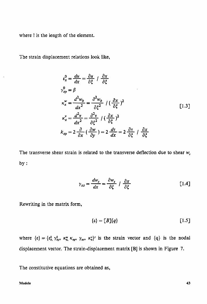
where | is the length of the element.

The strain displacement relations look like,

0_ du _ du , ox

ox ay OE! BE

Vay = B

* dx? gg? °° 88 [1.3]

v_ dv _ av ,, ox ne ak lar)

a2 (OW) Gu Ht OX Kay = 2G OG, = 2 2a | Be

The transverse shear strain is related to the transverse deflection due to shear w,

by:

dw, ow, Ox

Rewriting in the matrix form,

{e} = [B]{q} [1.5]

where {c} = {e2 y&, KY Ky, Yer KY} is the strain vector and {q} is the nodal

displacement vector. The strain-displacement matrix [B] is shown in Figure 7.

The constitutive equations are obtained as,

Models 43

- - - -

Ny Ay Aig By Big YA\| & Ai2 By

Nyy Aig Aes Bye Bes YAg| vxy Ar, Bre |

mrt = By, Bye Dy Dye YB, jer h + Bir D2 1 [1.6]

Myy Big Bes Pio Deo YBe| Kxy Bog Dos | ”

M: YA, YAg YB, YB, YD | Ke YA, YB,

The A’s, B’s and D’s are defined by analogy with the Classical Lamination

Theory [98] as:

5b ntl 2 =k

Ay = (24 — 24-1) Oy4y b —3k=l

5b ; n+l 2 = - By=|*° > De -%-VQGY t= 1,....6 [1.7] 226 b ; n+] 2 3. 3 mk

Ds=\ OF »~@ — 2) Qgdy - > k=] 2

and the terms pertaining to the lateral bending deflection are :

Models 44

b ntl

YA;= |? yd (ee - 2%) Oi b

-> k=]

b y n+1 2 2_ 2 yak ; YB, = oy Dee Oty j=1,...,6 [1.8]

-2° xl 2 5b ntl

YD=|? yD e—4Ony -2 2

where n is the total number of plies and z, is the coordinate of the top surface of

the k-th ply, numbered from the top down.

The transverse shear deformation is included in this formulation by splitting the

transverse deflection in two parts :

w= Ww, + W, [1.9]

w, is evaluated following Timoshenko’s method in which the transverse shear

force-strain relation is :

Nyxz = KA gay xz [1.10]

A,, is the transverse shear stiffness :

Models 45

Aga = (24 — 21) Gt34y [1.11]

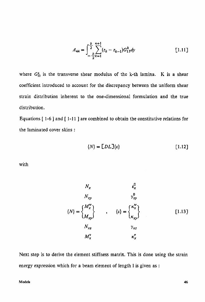
Where Gj, is the transverse shear modulus of the k-th lamina. K is a shear

coefficient introduced to account for the discrepancy between the uniform shear

Strain distribution inherent to the one-dimensional formulation and the true

distribution.

Equations [ 1-6 ] and [ 1-11 ] are combined to obtain the constitutive relations for

the laminated cover skins:

{N} = LDL ]{e} [1.12]

with

Ny ey

Nyy Vey

My Ky w=} | = 11.13]

Myy Ky

N yz Yxz

M, Ky

Next step is to derive the element stiffness matrix. This is done using the strain

energy expression which for a beam element of length | is given as:

Models 46

vat { ‘fey (N}dx [1.14] 2 0

where [k], the element stiffness matrix, is given by :

tk = | Tayo cela [1.15]

Incremental Stiffness Matrix

At this point we add the effect of rotation to the stiffness matrix. Observe that

the incremental matrix is derived from a linear analysis, i.e. assumption of small

deflections and rotations and, of course, small strains. Assuming a constant force

along the chord of the beam at any cross-section, the strain energy contribution

due to the centrifugal force acting on the beam is,

b ‘ 2 ! g If’, ;@

Ucentri = ri fas y)(SEY dx dy + > |e BY ote] -+ |

where,

Models 47

w(x, y, t) = w,(x,t) + w,(x,t) — yt(x,t) [1.17]

On substituting [ 1.17 } in [ 1.16 ] and assuming f, to be a function of x only and

for a uniform beam,

Ow Ow fawn WA F, (sr 2 *dx' + uw ax 7 )>dx’

1 Fi = )*dx’ t +5 Ele e ye + $f pry) artis] it F, (& » dx"

The expression for the centrifugal force F, and the incremental stiffness matrices

are given in the Appendix A. Here x’ is a dummy variable along the beam axis.

The effective stiffness matrix of the element is obtained on adding the stiffening

effect due to rotation to the original stiffness matrix [ 1.15 ]

Elemental mass matrix is obtained through the kinetic energy expression.

Neglecting rotatory inertia, the kinetic energy of the beam can be written as:

l

T= | oA ae dx + +f pa( yd + +f pa(-4- A yrgy 54.19]

Models 48

Using [ 1.17 ] expression for the kinetic energy is obtained as :

1 .2 .2 2 wt T= > pA[wy(x) + wi(x) + u(x) + v(x) ]dx

“0

if? ae 1 {' 2 + > 2pA[w,(x)w,(x)]dx + > | Ji*dx [1.20]

“0 0 /

++ | arpA(iyt + w,t)dx 2 Jo

where p is the material density, A(x) is the cross-sectional area of the beam, J(x)

is the polar mass moment of inertia of the section and r(x) is the offset between

the reference line and the center of gravity position. A more complete expression

for the Kinetic Energy leads to terms due to Coriolis and gyroscopic forces.

Following expressions for the element mass matrix components obtained in terms

of the interpolation polynomials :

for w,,w,,U and v:

my = f'pA(X)N)N(x)dx

fort:

my = fI(X)NC)N(x)dx [1.21]

coupling between w, and w, m= {'pA(x)N(x)N(x)dx

coupling between t and w,w,: my = fir(x)pA(x)N(x)N(x)adx

Models 49

Static Deflection and Free Vibration Analysis

At this stage of analysis we have the total stiffness and the mass matrix. Hence

we can go ahead with static analysis or we can find the natural frequencies and

mode shapes of the structure depending on the need.

The static deflection equation :

[K]{q} = (F} [1.22]

where [K] is the assembled structure stiffness matrix, {q} the total nodal

displacement vector and {F} the total nodal load vector. Eqn. [ 1.22 ] is solved

by the IMSL subroutine DLSLRG for the nodal displacements given {F}.

The equations of motion of the structure are obtained from Lagrange’s equations

and for harmonic oscillations are :

[LK] — w°[M] ]{q} = {0} [1.23]

where [M] is the assembled structure mass matrix and qw is the oscillation

frequency. This eigenvalue problem is solved with the help of the IMSL

subroutine DGVCRG. This code using 24 d.o.f. element for static and free

vibration analysis is called AE24.

Models 50

Aerodynamic Model

The strip theory was developed with the sole aim to analyze a three dimensional

wing with a two dimensional approach. Modified strip theory as developed by

Yates [ 99 - 103 J, is basically Theodorsen’s technique ( as discussed earlier ),

taking into account finite span of the wing oscillating ( sinusoidally ) in

compressible flow conditions. Main modifications being,

1. Arbitrary section lift - curve slope C, = C, (y) used instead of 2 z.

2. Arbitrary section aerodynamic center a, = a,(y) used instead of quarter -

chord.

3. The circulation function of Theodorsen is modified on the basis of 2-D

compressible flow theory to account approximately for effects of

compressibility on the magnitudes and phase angles of the section lift and

moment vectors.

The resulting expressions for the lift and moment are given in[ 7 ]. The principle

of virtual work is used to derive the aerodynamic matrix,

l l

éW = | dwLdx + { étMdx [1.24] 0 0

Models 51

aw = [[{dq}'NyLyNG + LNG + LAN + LYNG} [1.25] 0

+ {5q}'N,(M,,Ni, + MyNg + M,N! + MLN1){q} lw7*dx

- (5a) (tal + LyNyNj-+ LiNyNi+ LyNyNo [1.26]

+ M,,N.Ni,+ MgN.Ni + M_N,N! + M N,N) )o7dx ]{q}

= {59}'w*La]{q} [1.27]

Nodal load vector equivalent to the distributed aerodynamic loading is

therefore:

2 w* [a] {q}

where [a] is the complex element aerodynamic matrix.

Solution for Aeroelastic results.

The equations of motion of the wing oscillating with frequency w in unsteady

flow are:

([K] — [M]w? — [A]w){g} = {0} [1.28]

Models §2

where [A], the assembled aerodynamic matrix, is a function of the flow speed V

through the reduced frequency k =o . These equations are solved for the

flutter speed and frequency, and for divergence speeds using the V - g method.

The procedure is explained in [ 7 ]. For the flutter boundary it is necessary to find

that value of structural damping g, which when added to the existing damping,

just prevents the structure from going into the instability region. While

divergence speed is characterized by the speed at which g goes abruptly to zero (

from negative ), simultaneously with the frequency of oscillation.

Models 53

Results

Results obtained from the present code for a number of problems found in the

literature are presented. One of the objectives of the present work was to make

changes in the model developed by Castel & Kapania [ 14 ], and validate these

changes. AE12 (code using 12 d.o.f. used in Ref. [ 14 ]), dealt with six degrees

of freedom at each node w,, w,, t and their derivatives. Present code, AE24, is

basically an expansion to use the formulation in its full potential, i.e. addition of

u, B, v and their derivatives to render a 24 d.o.f. finite element. Each of these

deformations can become significant while dealing with anisotropic materials.

To validate this transformation some of the cases dealt with in [ 14 ] ( and some

others ) are reconsidered. Having verified the formulation and coding for the

stiffness, mass and the aerodynamic matrices through static, free vibration and

aeroelastic results respectively, the effects of centrifugal force on the static and

dynamic characteristics is studied.

Results 54

The results are hence divided into two parts, the first dealing with the validation

of the new expanded code and the second with the results obtained from the

rotating beam analysis.

Results 55

Validation

Static deflections

In the first case shear deflection for an isotropic beam under tip loading is

analysed. Material is aluminum and results are obtained and compared for the

case K = 0.667 and 0.867. Comparisons are made with exact solution due to

Timoshenko [ 105 ], and other references cited in Table 1.

A symmetrically laminated cantilever beam under the end load P, is next studied

and the distribution of tip deflections, both due to bending and shear

deformation, and twist are obtained using one element. The plotted values of the

delections are for the non - dimensionalized parameters

47 3 Wy WK Dag PPd,e Pld, ?P!

so that they are equal to unity at the tip. d,, and d, are the flexural compliances.

The properties of the beam [45,/ —45,], are the same as given in the reference

[ 106 ]. The results as shown in Figure 9 are in good agreement with ones

presented in [ 106 ].

Results 56

Finally in the static analysis, a beam consisting of top and bottom flat laminated

skins rigidly connected as shown in Figure 10 with unidirectional layer of

orthotropic material oriented at an angle @ from the spanwise axis, is considered.

The material properties of the laminae are as follows: E, = 6.9 x 10! N/m?,

E, = 5.0 x 10° N/m?, v1. = 0.30, Gy. = 1.5.x 10!° N/m?, p = 2.71 x 10? kg/m’.

Four elements were used to model and the analysis is done for the tip deflection

under a vertical tip load P = 200 N. The results obtained agreed well with the

ones in [ 14 ] over the entire range of values of the fibre angle @ as depicted in

Figure 11. The variatons are due to the different boundary conditions due to

additional degrees of freedom.

Free Vibrations

One example each from isotropic, and composite laminated structures ( one each

for symmetrical and unsymmetrical laminations ) were run.

Aluminum plates of dimension 6’ x 3” x 0.0416’, is used to perform the

analysis. Values for the bending and torsion frequencies, given in Table 2 match

well with the ones obtained in [ 109 ] confirming that plate analyzing capacity of

the code.

Results 57

Abarcar and Cunniff [ 110 ] presented results for the free vibrations of high

aspect ratio cantilever beams of unidirectional fiber reinforced composite

material. The beam length is 1 = 7.5 in, its width is b = 0.5 in and its thickness

is h = 0.125 in. The material properties are £,, = 18.7x10° psi,

Ey. = 1.36x 10° psi v,. = 0.3, G, = 0.7479 x 10° psi, G,; = 0.624 x 10° psi,

p = 0.1449 x 10-3 lb — sec? /in’.

The frequencies obtained using 3,4,8 and 9 finite elements to model a 30 ° off-axis

beam are shown in Table 3 and are found to agree well with those of Reference

[ 110 ]. We note a good convergence of results for the first four modes.

For unsymmetrically laminated panels, Thornton [ 111 ] evaluated the natural

frequencies of unsymmetric cantilevered Boron/Epoxy panels. The panels were

square (L = b = 8 in, h = 0.046 in), with the following material properties :

E, = 23.3x 10° psi, £, = 1.81 .x10° psi, v,. = 0.21, G,, = 0.98 x 10° psi,

p = 0.174 x 10-3 lb-sec?/ in* .

Eight plies constituted each panel, the four bottom plies being oriented at 0 °

while the top four plies were oriented at an off-axis angle to obtain the desired

bending-stretching coupling. The [ 45, / 0,], panel was modeled using 4 elements

to obtain the results presented in Table 4. The present formulation yields better

results for the first four modes than the 12 d.o.f. model from Ref. [ 14 ], when

compared to the experimental results presented in reference in [ 111 ].

Results 58

Aeroelastic results

Reference [ 112 ] presents analytical and experimental results for unswept

laminated cantilever plates. Two - dimensional unsteady aerodynamics is used in

conjunction with strip theory. Figure 12 shows that values obtained from

present study match well with [ 112 ], and are quite the same as [ 14 ]. Reason for

discrepancy can be attributed to one - dimensional nature of modeling of a plate

in the AE24 and also since it does not account for camber effect unlike [ 112 ].

For the box - beam Figure 10 ,the stability boundaries obtained from AE24 are

the same as presented in reference [ 14 ], and also match well with those presented

in reference { 113 ] as shown in Figure 13.

Results from the rotating beam.

We observe that the analysis using AE24 behaves more or less like the analysis

using the code AE12 of Ref. [ 14 ]. The incremental matrix introduced in the

code from a linear analysis of the rotating composite beam is now verified. The

pattern to be followed is the same as that of the first part i.e. static, free vibration

and lastly aeroelastic analysis, now with the effect of rotation.

Results 59

Static deflections.

The effect of rotation on a composite plate under a constant transverse tip load

is studied. The plate is a symmetrical Graphite/Epoxy [ 6,/0 ], considered in

reference [ 112 ]. The reference work, however, does not deal with static analysis.

Plate has the dimensions of J/= 0.305m b = 0.076 m and

h = 0.804x10-?m and the properties are, £,, = 98.0x 109 N/m?,

Ei. = 7.9.x 109 N/m2, Vio = 0.28, Gi. = 5.6 x 10° N/m?,

Gi; = 5.6x10°N/m2, p = 1.52x 10°?kgm-3.

The results obtained are shown in Figure 14. As expected centrifugal forces

increase the stiffness of the plate and tip deflections decrease. Higher values of @

mean a lower value of flexural stiffness, a fact clearly represented in the figure.

We notice higher values of deflection with increasing 6.

Free Vibration.

Beginning with the isotropic case, the first natural frequency is plotted against the

angular velocity of an aluminum rotating beam. The values plotted are non -

pals

ETS angular velocity of rotation and the natural frequency of vibration of the beam

Alt dimensionalized parameters defined as, Q( ), and w( —), for the

respectively. Comparisons are made with several works namely that of Kumar [

114 ], Wang [ 115 ], Bhat { 116 ] which used Mykelstad, Galerkin and Raleigh -

Ritz methods respectively. Comparison as can be seen in Figure 15 is good.

Results 60

Effect of the radius of the hub on the vibration characteristics of the blade is also

studied. Values are compared with those in reference [ 104 ] ( which also uses a

finite element technique ) and the comparison is good. As shown in Figure 16

for R values of 2.4 and 6 ( which are more true for turbine blades for example ),

higher hub radius to blade length ratio seem to render a stiffer structure.

A similar study is carried out for a Graphite/Epoxy plate considered in [ 110 J.

The plot of angular velocity vs first natural frequency of vibration is presented in

Figure 17 for different values of fiber orientation. The behaviour is similar to the

isotropic one with plate getting more flexible for higher values of fiber angle as

evident from lower values of frequency of vibration.

Figure 18 shows the effect of R on the free vibration characteristics of the box

beam. The non-dimensionalized parameter used here is of the form,

pAPh} pAPh} Q ( Dif ), and w ( DT ).

Results 61

Conclusions and Recommendations for Future Work

The code for 24 degrees of freedom, AE24, was successfully run and validated

using several examples. It seemed to perform better than the code AE12[ 14 ], for

the unsymmetrical specimen. Linear static and free vibration analysis yielded

results consistent with expected ones. Both rotation and fiber orientation are seen

to play a prominent role in the determination of the static deflections and the

natural frequencies of vibration.

As seen in the literature survey, the state of art structural model used in the

aeroelastic analysis of helicopter rotors is much more complex than the one used

in the present work.

Conclusions and Recommendations for Future Work 62

There is a need for developing a non-linear analysis technique for the structural

model. Care should be taken to account for the Coriolis and gyroscopic terms in

the mass and the stiffness matrices. Warping, which is very significant in

anisotropic materials has to be accounted for in a more efficient way. Stemple

and Lee [ 70 ] have suggested a coupled analysis for the cross-section warping and

the bending, torsion, and extension of the beam. This could be introduced in the

present FEM model. Also features like pretwist, droop and precone have been

found to be important for the helicopter rotor analysis.

A preliminary aeroelastic analysis for helicopter rotors could be carried out using

either a modified-strip theory approximation for unsteady airloads (this model

already exists in AE24) or a quasi-steady approximation in conjunction with a

simple induced flow model [ 44 ]. The state of art classical unsteady aerodynamic

approach is the State-Space or Finite-State representation (i.e. in the time

domain) of the equations of motion [ 85, 118 ].

Conclusions and Recommendations for Future Work 63

References

References

Bisplinghoff, R.L., and Ashley, H., Principles of Aeroelasticity, John Wiley and Sons, Inc., NY, 1962.

Collar, A. R., “The Expanding Domain of Aeroelasticity,” Journal of Royal Aeronautical Society, Vol. 50, August 1946, pp. 613 - 636.

Duncan, W.J., “Inroductory Survey,” AGARD, Manual of Aeroelasticity, August 1959, pp. 1 - 51.

Gessow, A., and Myers, G., C., Jr., Aerodynamics of Helicopters, The Macmillan Co., NY, 1952.

Bramwell, A.R.S., Helicopter Dynamics, John Wiley & Sons, NY, 1976.

Loewy, R.G., “Review of Rotary-Wing V/STOL Dynamic and Aeroelastic Problems,” Journal of American Helicopter Society, Vol. 14, 1969, pp. 3 - 23.

Dowell, E., H., “A Modern Course in Aeroelasticity,” Sijthoff & Noordhoff, Alphen aan den Rijn, The Netherlands, 1978.

Marr, R., L., Blackmann, S., Weiberg, J., A., and Schroer, L., G., “Wind Tunnel and Flight Test for XV-15 Tilt Rotor Research Aircraft,” Paper No. 79-54, Proceedings of the 35th Annual National Forum of the American Helicopter Society, Washington, D.C., 1979.

Bilger, J.. Marr, R., L., and Zahedi, A., “Results of Structural Dynamic Testing of the XV-15 Tilt Rotor Research Aircraft,” Journal of the American Helicopter Society, Vol. 27, No. 2, April 1982, pp. 58 - 65.

10.

12.

13.

14.

15.

16.

17.

18.

19,

20.

21.

22.

References

Jenny, D., S., “ABC Aircraft Developement Status,” Paper No. 8, Proceedings of the 6th European Rotorcraft Forum, Bristol, England, September 1980, pp. 8.1 - 8.6.

Linden, A., and Ruddell, A., “An ABC Status Report,” Proceedings of the 37th Annual National Forum of the American Helicopter Society,New Orleans, May 1981, pp. 72 - 87.

Williams, R., M., “Application of Circulation Control Rotor Technology to a Stopped Rotor Aircraft Design,” Vertica, Vol. 1, No. 1, 1976, pp. 3 - 16.

Potthast, A., J., “X-Wing Stability and Control Developement and Wind Tunnel Demonstration Tests - Helicopter Conversion and Fixed Wing flight,” Paper No. 80-27, Proceedings of the 36th Annual National Forum of the American Helicopter Society, Washington, D.C., May 1980.

Castel, F., and Kapania, R.,K., “A Beam Element for Aeroelastic Analysis of Damaged and Undamaged Wings.”, A Report for CCMS (Virginia Tech) CCMS 88-13.

Dat, R., “Aeroelasticity of Rotary-Wing Aijrcraft,” Helicopter Aerodynamics and Dynamics, AGARD Lecture Series, No. 63, Chapter 4, 1973.

Hohenemser, K., H., “Hingeless Rotorcraft Flight Dynamics,” Agardograph, No. 197, 1974.

Ormiston, R., A., “Investigation of Hingeless Rotor Stability,” Vertica, Vol. 7, pp. 143 - 181.

Friedmann, P., P., “Recent Developements in Rotary-Wing Aeroelasticity,” Journal of Aircraft, Vol. 14, 1977, pp. 1027 - 1041.

Friedmann, P., P., “Formulation and Solution of Rotary-Wing Aeroelastic Stability and Response Problems,” Vertica, Vol. 7, No. 2, 1983, pp. 101 - 141.

Friedmann, P., P., “Recent Trends in Rotary-Wing Aeroelasticity,” Vertica, Vol. 11, No. 1, 1987, pp. 139 - 170.

Reichert, G., “ Helicopter Vibration Control - A survey, ” Vertica, Vol. 5, 1981, pp. 1 - 20.

Loewy, R., G., “Helicopter Vibrations: A Technological Perspective,” Journal of American Helicopter Society, Vol. 29, 1984, pp. 4 - 30.

65

23.

24.

25.

26.

27.

28.

29.

30.

31.

32.

33.

34.

References

Johnson, W., “ Recent Developements in the Dynamics of Advanced Rotor Systems - Part I,” Vertica, Vol. 10, 1986, pp. 73 - 107.

Johnson, W., “Recent Developements in the Dynamics of Advanced Rotor Systems - Part II,” Vertica, Vol. 10, 1986, pp. 109 - 150.

Miao, W., “Influence of Pitch - Axis Location and Orientation on Rotor Aeroelastic Stability,” Vertica, Vol. 11, No. 1/2, 1987, pp. 171 - 185.

Ormiston, R.,A., Warmbrodt, W., G., Hodges, D.,H., and Peters, D., A., “Survey of Army / NASA Rotorcraft Aeroelastic Stability Research,” NASA TM - 101026, October, 1988.

Friedmann, P., P., “ Helicopter Rotor Dynamics and Aeroelasticity - Some Key Ideas and Insights, ” Third Workshop on Aeroelastic Stability Modelling of Rotorcraft Rotor Systems, March 12 - 14, Durham, NC, 1990.

Houbolt, J., C., and Brooks, G., W., “Differential Equations of Motion for Combined Flapwise Bending, Chordwise Bending and Torsion of Twisted Non - uniform Rotor Blades,” NACA Report 1346, 1958.

Friedmann, P., P., and Tong, P., “Dynamic Nonlinear Elastic Stability of Helicopter Rotor Blades in Hover and in Forward Flight,” NASA CR - 114485, May 1972.

Arcidiacono, P., J., “Steady Flight Differential Equations of Motion for a Flexible Helicopter Blades with Chordwise Mass Unbalance,” USAAVLABS TR68 - 18A, Vol. I, February 1969.

Hodges, D., H., and Dowell, E., H., “Nonlinear Equations of Motion for Elastic Bending and Torsion of Twisted Non - uniform Blades,” NASA TN D - 7818, 1974.

Friedmann, P., P., “Influence of Modeling and Blade Parameters on the Aeroelastic Stability of a Cantilevered Rotor,” AJAA Journal, Vol. 15, February 1977, pp. 149 - 158. .

Dowell, E., H., Traybar, J., and Hodges, D., H., “An Experimental Theoretical Correlation Study of Nonlinear Bending and Torsion Deformations of a Cantilever Beam,” Journal of Sound and Vibration, Vol. 50, 1977, pp. 533 - 544.

Hodges, D., H., Ormiston, R., A., and Peters, D., A., “On the Nonlinear Deformation Geometry of Euler Bernoulli Beams,” NASA TP - 1566, 1980.

66

35.

36.

37.

38.

39.

40.

41.

42.

43.

44.

45.

References

Alkire, K., “An Analysis of Rotor Blade Twist Variables Associated with Different Euler Sequences and Pretwist Treatment,” NASA TM - 84394,

1984.

Shamie, J., and Friedmann, P., “Effect of Moderate Deflections on the Aeroelastic Stability of a Rotor Blade in Forward Flight,” Proc. Third European Rotorcraft and Powered Lift Aircraft Forum, Aix - en - Provence, pp. 24.1 - 24.37, 1977.

Celi, R., and Friedmann, P.,P., “Rotor Blade Aeroelasticity in Forward

Flight with an Implicit Aerodynamic Formulation,” AJAA Journal , Vol. 26, No. 12, 1988, pp. 1425 - 1433.

Hodges, D., H., “Nonlinear Equations for the Dynamics of Pretwisted Beams Undergoing Small Strains and Large Rotations,” NASA TP - 2470, 1985.

Hodges, D., H., “Nonlinear Beam Kinematics for Small Strains and

Finite Rotations,” Vertica, Vol. 11, No. 3, 1987, pp. 573 - 589.

Danielson, D., A., and Hodges, D., H., “A Beam Theory for Large

Global Rotation, Moderate Local Rotation and Small Strain,” Journal

of Applied Mechanics, Vol. 55, pp. 179 - 184.

Kane, T., R., Likins, P., W., and Levinson, D., A., “Spacecraft

Dynamics,” McGraw-Hill, 1983.

Bauchau, O., A., and Hong, C., H., “Large Displacement Analysis of Naturally Curved and Twisted Composite Beams,” AJAA Journal, Vol. 25, No. 11, 1987, pp. 1469 - 1475.

Hodges, D., H., Hopkins, A., K., Kunz, D., L., and Hinnant, H., E.,

“Introduction to GRASP - General Rotorcraft Aeromechanical Stability Program - A Modern Approach to Rotorcraft Modeling,” Proc. 42nd Annual Forum of American Helicopter Society, Washington D. C., 1986, pp. 739 - 756.

Sivaneri, N. T., and Chopra, I., “Dynamic Stability of Rotor Blade Using Finite Element Analysis,” AJAA Journal, Vol. 20, 1980, pp. 716 - 723.

Sivaneri, N. T., and Chopra, I., “Finite Element Analysis of Bearingless Rotor Aeroelasticity,” Journal of American Helicopter Society, Vol. 29, 1984, pp. 42 - 51.

67

46.

47.

48.

49.

50.

51.

52.

53.

54.

55.

56.

57.

References

Friedmann, P. P., and Straub, F., “Application of the Finite Element Method to Rotary - Wing Aeroelasticity,” Journal of American Helicopter Society, Vol. 25, 1980, pp. 36 - 44.

Fu, C., and Wang, S., “Aeroelastic Stability of a Rotor by Lifting Surface Theory and Finite Element Method,” Proc. //th. European Rotorcraft Forum, London, Paper No. 68, 1986.

Hodges, D., H.,“ Review of Composite Rotor Blade Modeling,” AIAA Paper 88 - 2249, Proc. AIAA / ASME / ASCE / AHS 29th Structures, Structural Dynamics, and Materials Conference, Williamsburg, Va, April 18 - 20, 1988, pp. 305 - 312.

Hong, C. H., and Chopra, I., “Aeroelastic Stability Analysis of a Composite Rotor Blade,” Journal of American Helicopter Society, Vol. 30, No. 2, 1985, pp. 57 - 67.

Hong, C. H., and Chopra, I., “Aeroelastic Stability Analysis of a Composite Bearingless Rotor Blade,” Journal of American Helicopter Society, Vol. 31, No. 4, 1986, pp. 29 - 35.

Panda, B., and Chopra, I., “Dynamics of Composite Rotor Blades in Forward Flight,” Vertica, Vol. 11, No. 1/2, 1987, pp. 187 - 209.

Bauchau, O., A., and Hong, C., H., “Finite Element Approoach to Rotor Blade Modeling,” Journal of American Helicopter Society, Vol. 32, No. 1, January 1987, pp. 60 - 67.

Bauchau, O., A., and Hong, C., H., “Nonlinear Composite Beam Theory,” Journal of Applied Mechanics, Vol. 55, March 1988, pp. 156 - 163.

Minguet, P., and Dugundji, J., “Experiments and Analysis for Structurally Coupled Composite Blades Under Large Deflections : Part ] - Static Behaviour,” AIAA Paper No. 89 - 1365 - CP, 1989.

Minguet, P., and Dugundji, J., “Experiments and Analysis for Structurally Coupled Composite Blades Under Large Deflections : Part II] - Dynamic Behaviour,” AIAA Paper No. 89 - 1366 - CP, 1989.

Hegemier, G., A., and Nair, S., “A Nonlinear Dynamical Theory for Heterogenous, Anisotropic, Elastic Rods,” AJAA Journal, Vol. 15, No. 1, 1977, pp. 8 - 15.

Mansfield, E. H., and Sobey, A. J., “The Fibre Composite Helicopter Blade , Part I : Stiffness Properties ( by E. H. Mansfield ) ; Part II :

68

38.

59.

60.

61.

62.

63.

64.

65.

66.

67.

68.

References

Prospects for Aeroelastic Tailoring ( by A. J. Sobey ),” Aeronautical Quarterly, May, 1979, pp. 413 - 449.

Mansfield, E., H., “ The Stiffness of a Two - Cell Anisotropic Tube,” Aeronautical Quarterly, Vol. 32, 1981, pp. 338 - 353.

Rehfield, L., W., “Design Analysis Methodology for Composite Rotor Blades,” AFWAL - TR - 85 - 3094, 1985.

Nixon, M., W., “Extension - Twist Coupling of Composite Circular Tubes with Applications to Tilt - Rotor Blade Design,” AIAA Paper No. 87 - 0772, 1987.

Hodges, R., V., Nixon, M., W., and Rehfield, L., W., “Comparison of Composite Rotor Blade Models : a Coupled Beam Analysis and an MSC / NASTRAN Finite Element Model,” NASA TM 89024, 1987.

Worndle, R., “Calculation of the Cross - Sectional Properties and the Shear Stresses of Composite Rotor Blades,” Vertica, Vol. 6, 1982, pp. 111 - 129.

Kosmatka, J., B., “Structural Dynamic Modeling of Advanced Composite Propellers by the Finite Element Method,” Ph.D. Dissertation, University of California, Los Angeles, 1986.

Giavotto, V., Borri, M., Mantegazza, P., Ghiringhelli, G., Carmaschi,

V., Maffloli, G., C., and Mussi, F., “Anisotropic Beam Theory and Applications,” Computers and Structures, Vol. 16, 1983, pp. 403 - 413.

Borri, M., and Mantegazza, P., “Some Contributions on Structural and Dynamic Modelling of Helicopter Rotor Blades,” Presented at U. S. Army Research Office Workshop on Dynamics and Aeroelastic Stability Modeling, Georgia Institute of Technology, Atlanta, Georgia, December 4-5, 1985.

Borri, M., and Merlini, T., “A Large Displacement Formulation for Anisotropic Beam Analysis,” Meccanica, Vol. 21, 1986, pp. 30-37.

Bauchau, O., A., “A Beam Theory for Anisotropic Materials,” Journal

of Applied Mechanics, Vol. 52, 1985, pp. 416 - 422.

Bauchau, O., A., Coffenberry, B., S., and Rehfield, L., W., “Composite

box -beam analysis : Theory and Experiments,” Journal of American Helicopter Society, Vol. 6, 1987, pp. 25 - 35.

69

69.

70.

71.

72.

73.

74,

75.

76.

77.

78.

79.

80.

81.

References

Lee, S., W., and Kim, Y., H., “A New Approach to Finite Element Modeling of Beams,” International Journal for Numerical Methods for Engineers, Vol. 24, 1987, pp. 2327 - 2341.

Stemple, A. D., and Lee, S., W., “Finite Element Model for Composite Beams with Arbitrary Cross - Sectional Warping,” A/AA Journal, Vol. 26, No. 12, December 1988, pp. 1512 - 1520.

Stemple, A., D., and Lee, S., W., “Large Deflection Static and Dynamic Finite Element Analysis of Composite Beams with Arbitrary Cross - Sectional Warping,” AIAA Paper 89 - 1363 - CP, 1989.

Gaonkar, G., H., and Peters, D., A., “Review of Dynamic Inflow Modeling for Rotorcraft Flight Dynamics,” AIAA - 86 - 0845, 1986.

Amer, K., B., “ Theory of Helicopter Damping in Pitch and Roll and Comparison with Flight Measurement,” NACA TN 2136, October 1948.

Sissingh, G., J., “ The Effect of Induced Velocity Variation on Helicopter Rotor Damping in Pitch and Roll, ”Aeronautical Research Council ( Great Britain ), A. R. C. Technical Report C. P. No. 101 ( 14, 757 ), 1952.

Carpenter, P., J., and Fridovich, B., “Effect of a Rapid Blade Pitch Increase on the Thrust and Induced Velocity Response of a Full Scale Helicopter Rotor,” NACA TN 3044, Nov, 1953.

Bisplinghoff, R., L., Ashley, H., and Halfman, R., L., Aeroelasticity, Addison - Wesley Publishing Company, 1955, pp. 251 - 281.

Glauert, H., “The Force and Moment on an Oscillating Airfoil, ” Br. A R. C., R. and M. 1242, 1929.

Theodorsen, T., “General Theory of Aerodynamic Instability and the Mechanism of Flutter,” NACA R 496, 1985.

Greenberg, J., M., “Airfoil in Sinusoidal Motion in Pulsating Stream,” NACA TN 1326, 1947.

Loewy, R., G., “ A Two Dimensional Approach to the Unsteady Aerodynamics of Rotary Wings, ” Journal of Aerospace Science, Vol. 24, 1957, pp. 81 -98.

Jones, W., P., “The Oscillating Airfoil in Subsonic Flow,” British

Aeronautical Research Council, R & M 2921, 1956.

70

82.

83.

84,

85.

86.

87.

88.

89.

90.

91.

92.

References

Timman, R., and van de Vooren, A., I., “ Flutter of a Helicopter Rotor Rotating in its Own Wake,” Journal of the Aerospace Sciences, Vol. 24, No. 9, September 1957, pp. 694 - 702.

Jones, W., P., and Rao, B., M., “Compressibility Effects on Oscillating

Rotor Blades in Hovering Flight,” Presented at the AIAA Structural Dynamics and Aeroelasticity Specialist Conference, New Orleans, Louisiana, April 16 - 17, 1969.

Hammond, C., E., and Pierce, G., A., “A Compressible Unsteady

Aerodynamic Theory for Helicopter Rotors,” Presented at the AGARD Specialist’s Meeting on “The Aerodynamics of Rotary Wings,” Marseille, France, September 13 - 15, 1972.

Friedmann, P., P., and Venkatesan, C., “Finite State Modeling of Unsteady Aerodynamics and its Application to a Rotor Dynamic Problem,” Presented at Eleventh European Rotorcraft Forum, Paper No.

72, London, England, September 10 - 13, 1985.

Drees, J.,. M., “A Theory of Airflow Through Rotor and its Application to Some Helicopter in Forward Flight,” Journal of the Helicopter Society of Great Britain, Vol. 3, No. 2, 1949.

Heyson, H., H., and Kotzoff, S., “Induced Velocities Near a Lifting

Rotor with Non - uniform Disk Loading,” NASA TR 1319, 1957.

Wang, Shi - Cun, “ Generalized Rotor Vortex Theory, Problems of

Helicopter Rotor Aerodynamics,” NASA TT F - 494, September 1967.

Miller, R., H., “Rotor Blade Harmonic Air Loading,” AJAA Journal,

Vol. 2, No. 7, July 1964, pp. 1254 - 1269.

Scully, M., P., “A Method of Computing Helicopter Vortex Wake Distortion,” MIT, ASRL TR138 - 1, June 1967.

Sadler, S., G., “Developement and Application of a Method for

Predicting Rotor Free Wake Positions and Resulting Rotor Blade Airloads,” NASA CR - 1911, Vol. I : Model and Results, NASA CR -

1912 Program Listing, 1971.

Gray, R., B., “ On the Motion Helical Vortex Shed from a Single - Bladed Hovering Helicopter Rotor and its Application to the Calculation of the Spanwise Aerodynamic Loading, ”Princeton University, Aero. Engineering Dept., Report No. 313, September 1955.

71

93.

94.

95.

96.

97.

98.

99.

100.

101.

102.

103.

104.

References

Shupe, N., K., “ A Study of the Dynamic Motions of Hingeless Rotored Helicopters,” Ph.D. Thesis, Princeton University, 1970.

Curtiss, H., C., Jr., and Shupe, N., K., “A Stability and Control Theory

for Hingeless Rotors,” Annual National Forum of the American Helicopter Society, Washington, D.C., May 1971.

Bousman, W., G., “An Experimental Investigation of the Effects on Aeromechanical Stability of a Hingeless Rotor Helicopter,” Journal of American Helicopter Society, Vol. 26, No. 1, January 1981, pp. 46 - 54.

Pitt, D., M., and Peters, D., A., “ Theoretical Prediction of Dynamic Inflow Derivatives,” Vertica Vol. 5, No. 1, March 1981, pp. 21 - 34.

Peters, D., A., and Ninh HaQuang, “Dynamic Inflow for Practical Application,” Journal of the American Helicopter Society, Vol. 33, No. 4, October 1988.

Jones, R., M., Mechanics of Composite Materials, McGraw - Hill, 1975.

Yates, E., C., Jr., “Calculation of Flutter Characteristics for Finite - Span Swept or Unswept Wings at Subsonic and Supersonic Speeds by a Modified Strip Analysis,” NACA RM L57L10, 1958.

Yates, E., C., Jr., “Use of Experimental Steady - Flow Aerodynamic Parameters in the Calculation of Flutter Characteristics for Finite Span Swept or Unswept Wings at Subsonic, Transonic, and Supersonic Speeds,” NASA TM X - 183, 1960.

Yates, E., C., Jr., “Subsonic and Supersonic Flutter Analysis of a Highly Tapered Swept Wing Planform Including Effects of Density Variation and Finite Wing Thickness and Comparison with Experiments,” NASA TN D - 4230, 1967. ( Supercedes NASA TM X - 764, 1983 )

Yates, E., C., Jr., “Modified - Strip Analysis Method for Predicting Wing

Flutter at Subsonic to Hypersonic Speeds,” Journal of Aircraft, Vol. 3, No. 1, January - February 1966, pp. 25 - 29.

Yates, E., C., Jr., “Flutter Prediction at Low Mass - Density Ratios with

Application to the Finite - Span Noncavitating Hydrofoil,” AIAA Paper No. 68 - 472, April - May, 1968.

Hoa, S., V., “Vibration of a Rotating Beam With a Tip Mass,” Journal of Sound and Vibration, Vol. 67, No. 3, 1979, pp. 369 - 381.

72

105.

106.

107.

108.

109.

110.

111.

112.

113.

114.

115.

116.

References

Timoshenko, S., P., Goodier, J., N., Theory of Elasticity, 3rd Edition, McGraw - Hill Book Company, New York, 1970.

Chen, A., T., and Yang, T., Y., “Static and Dynamic Formulation of a Symmetrically Laminated Beam Finite Element for a Microcomputer,” Journal of Composite Materials, Vol. 19, September, 1985.

Archer, J., S., “Consistent Matrix Formulations for Structural Analysis Using Finite Element Techniques,” AJAA Journal, Vol. 3, 1965, pp. 1910 - 1918.

Popov, E., P., “Jntroduction to Mechanics of Solids,” Prentice-Hall, Inc. Englewood Cliffs, N.J., 1968, pp. 482 - 487.

Crawley, E., F., “The Natural Modes of Graphite/Epoxy Cantilever Plates and Shells,” Journal of Composite Materials, Vol. 13, July 1979, pp. 195 - 205.

Abarcar, R., B., and Cunniff, P., F., “The Vibration of Cantilever Beams of Fiber Reinforced Material,” Journal of Composite Material, Vol. 6, 1972, pp. 504 - 517.

Thornton, E., A., “ Free Vibrations of Unsymmetrically Cantilevered Composite Panels,” Shock and Vibration Bulletin, Part 2, 1976, pp. 79 - 84.

Hollowell, S., J., and Dugundji, J., “Aeroelastic Flutter and Divergence of Stiffness Coupled, Graphite/Epoxy, Cantilevered Plates,” AIAA Paper 82 - 0722, May 1982.

Bergen, F., D., “Shape Sensitivity Analysis of Wing Dynamic Aeroelastic Response,” M. S. Thesis, Virginia Polytechnic Institute and State University, July, 1988.

Kumar, R., “Vibrations of Space Booms Under Centrifugal Force Field,” Transactions of the C.A.S.1., No. 7, 1974, pp. 1 - 5.

Wang, J., T., H., Mahrenholtz, O., and Bohm, J., “Extended Galerkin’s Method for Rotating Beam Vibrations Using Legendre Polynomials,” Solid Mechanics Reviews, 1976, pp. 341 - 365.

Bhat, R., B., “Transverse Vibrations of a Rotating Uniform Cantilever Beam with Tip Mass as Predicted by Using Beam Characteristic Orthogonal Polynomials in Raleigh-Ritz Method,” Journal of Sound and Vibrations, Vol. 105, No. 2, 1986, pp. 199 - 210.

73

117.

118.

References

Weisshaar, T., A., “Divergence of Forward Swept Composite Wings,” Journal of Aircraft, Vol. 17, No. 6, 1980, pp. 442 - 448.

Leishman, J., G., Nguyen, K., Q., “State-Space Representation of Unsteady Airfoil Behavior,” AJAA Journal, Vol. 28, No. 5, May 1990, pp. 836 - 844.

74

Figures and Tables

Figures and Tables 75

Table 1. Maximum deflection w, in Pik? 4El

due to shear deformation only

K = 0.667 K = 0.867

Exact Soln. [ 105 ] 1.33 -

Ref. [ 106 ] 1.33 1.0

Ref. [ 107 | 1.34 1.17

Strain Energy | 108 ] 1.33 1.04

24 d. o. f. 1.33 1.023


Table 2. Natural frequencies for the Aluminium plate

Mode Ref. [| 109 } 24 dof.

f Hz. f Hz

I Bending 37.6 37.5

] Torsion 158.3 143.9

II Bending 234.9 235.5

II Torsion 518.8 431.83

III Bending 658.1 663.7


y L78i $9681

9SLLI CLLLI

008! 60677

v

L'vc6 6S16

1016 {016

8°816 1'@?6

t

SICe €6ce

6L7t 6 LCE

£'87e C6ce

¢

Les Les

9¢S 9S

9S -

9S

I

“ZH §

“ZH YS

"ZH J

“ZHI S “ZIT S

“ZH

SJUIWIIJD 6 |

SJUdUIDID g |

spuduaja p |

syudWaa ¢ |

“ONY DPOF]

lout) “Jou

juowniodxy fort)

Ju Yonsipesd

YAO AA HUISIAT

ureag saaajuey

dxodq/ayydery sixy-yO

$39383q O¢

BJO satquanbaiy

pesnyeN, =

“€ F198 L

78 Figures and Tables

Table 4. Natural frequencies of a [ 45, /0, ]; Boron/Epoxy plate

24 dof. Ref. | 14] Experiment Ref{ 111 J

Mode No. f, Hz f, Hz f, Hz

1 23.0 25.0 24.4

2 47.6 41.7 $5.1

3 131.6 117.0 141.0

4° 156.4 143.5 157.0


, a)

ROL jl PITCH

DROOP

Ce ee — J PRECONE

Figure 1. a)A typical Helicopter configuration b) defining precone and droop

b)


AXIS

AXIS OF

ROTATION

HINGELESS ARTICULATED

BEAM FLEXURE

LEADING BEARINGLESS

PITCH LINK

Figure 2. Various hub configurations of rotor blades, Reference [ 7 |


Z, K

4;

pe,

Figure 3. Typical Helicopter rotor configuration: a) Undeformed , b) Deformed position of the

elastic axis


Q)

erOW INDUCED K FLOW THEORY |.

@&eocenerseeoeece 4

CONTFOLS ATTACK, UFTING THEORY | CRORATON OR

AIRF O&_ AEROOYNAMICS |

GLADE MOTIONS

ROTOR OYNAMICS }<

BOOY DYNAMICS

Figure 4. Block diagram of inflow dynamics


Figure 5. Built-up blade model.

\—z-+ STRINGER


Figure 6. Element degrees of freedom


auem, 2]/LN, 0 ‘ @ e

0 0 6 9 ‘ °

0 0 4ju?n", 4jt'w, 4 ¢

(CB) =

0 0 o e 6 °

0 0 6 @ = 2/LN, ILN;

0 e ¢ ¢ 0 é

2/LNy 2/LNy; 6 e

Q e ¢ ®

6 0 4/L'n, 4/1'N,

Q 0 9 0

¢ e e 0

e 0 8 @

Figure 7. Strain-Displacement Matrix

Figures and Tables

¢ oe 6

° oN Of,

0 ee e@

4/LN", 4]LN", @ 6

¢ o @¢ @

Q ee

e ® e e

® 6 6 e

@ 6 9 6

° 6 4/LN’, 4/LN, 0

2/LN’; 2/LN, 6 0

e e ® e

@ 4/0N, Lh,

e e 6

Ne ¢

e 6 @

e 0 0

6 . 8

4

0 afin, 4/L?N,

|

86

Figure 8. Configuration of a rotating beam.


NONDIMENSIONALIZED DEFLECTIONS

o 92

9 9

9 9

9 oo

= Ne fe

oe YY

® ©

°

Figure 9.

0.2 . 0.3 0.4 0.5 0.6 0.7 . 0.8 . 0.9 7 1.0

X / L BEAM LENGTH

i ese BENDING(AE2Z4 ) 1+ SHEAR AEZ4 )

o-2-» TWISTCAE2Z4 } eea BENDING REF.(106 eee SHEAR REF.( 106) oe TWIST REF.(106)

Distribution of deflections due to bending and shear deformations and twisting angle for a

16 ply (45, / —45,], under a tip load P.


-05m

05m rigid connectors

L

we

3 Am ™y

> <

Figure 10. Box Beam Geometry Ref. | 14 ]


).

cna ns sti

te Caen

t

( METERS

Ge

Ct

af» »

TIP

DEFLECTION

bunt

-

0 T - T ” T ¥ T ¥ T ¥ tT ¥ " ' " . ~

0 10 20 30 40 5 60 70 80

FIBER ANGLE — REF. 113 ~—— REF. 14 eos PRESENT WORK

Figure 11. Box Beam Tip Deflection Under a Tip Load

Figures and Tables

40; =

355

DS (M/S

8 CRITICAL SPEE

Nn on °

FIBER ANGLE (DEG) +++ DIVERGENCE.(112) ooD FLUTTER, ( 8&0 DIVERGENCE AE24 + FLUTTER Ae

Figure 12. Critical Speed of an Unswept Graphite/Epoxy Plate, ( 6, / 0),

Figures and Tables

2 2 >

—

91

150 7F v

1207

wo oO

CRITICAL SPEEDS

( M/S

) mo oO

S

FIBER ANGLE (DEG) +++ DIVERGENCE .(113) e248 FLUTTER.(113) 8)» DIVERGENCE AE24 ooo FLUTTER AE24 ++ 5 >) 6

Figure 13. Flutter and Divergence Speeds of an Unswept Box Beam


FLECTION

NON—DIMENSIONAL

DE

1.23

o

oO ©o o

Oo a

on

oe

9

Oo ND 0.0

0 15 30 45 60 75

FIBER ANGLE ( DEG )

oo 0 RPM +++500 RPM 2» 1000 RPM

Figure 14. Tip deflection vs 6 for a rotating ( 6, / 0 ), plate.

Figures and Tables

90

93

4 GW (PA(L**4)/EI) 2

A

ihn

a

Sate

ah

it te

a o

2;

of § ied 7 oe q " q ” q * é * t ” qT “

0 1 2 3 4 5 6 7 8 9 10 d

A(PA(L**4)/EI)2 — REF. (115) ----- REF. (116) —— REF. (114) oe» PRESENT WORK

Figure 15. Variation of first natural frequencies of vibration with angular velocity for an isotropic beam, R=0.


FREQUENCY

PARAMETER

NY #=W

3 ~A

oO +

&® BS

& 8

*%

‘e

“Se

ai 2

oe @

£ e af

eo

ee

ah

N \

*

04

o 1 2 3 4 85 6 7 8 $ 1 ANGULAR VELOCITY PARAMETER

+++RBAR 0 AE24 +++ RBAR 0 HOR eee RBAR 2.4 RE24 e--« RBAR 2.4 HOR ®50 RBAR 6 RE24 0-6-8 RBAR 6 HOR

Variation of first natural frequencies of vibration with angular velocity for isotropic beam Figure 16. with different values of R


3000 ;

x

Pa

aa

N o ° ‘ ‘

“

vociatnttimnbe

ANGULAR FREQUENCY

2000; q

]

1500; y q a

4 7”

a q a . 4 0

5

1000: ue *

°° 4

q 4q

inSbefendiee te

: 01a aaa aaa —— — : 0 500 1000 1500 2000 2500

0 ----0 DEG --- 30 DEG eoo60 DEG + +90 DEG

Figure 17. Variation of first natural frequencies of vibration with angular velocity for the Graphite/Epoxy plate R = 0.


6 a

q

§

4

q

q be)

4

' D

4 e

oe

55 ° ° .

‘ d rd

@o

e o

of q Y ,

4 o 4 o 4 7

Pa id e + e °

o ° a * “ °

4 4 ° . ¢ ° ¢

q a ao ° . ” *

¢ * e

&% 4 s o ° ” * ‘ b) ‘ 4 ° ra

’ ° o 4 a o” ra

roe 4 yg o? .

hd ’ q eo ° a~

ra * *

°” ¢ 4 e +

4q o” a”

? * ¢ 4 Ig” ° *

‘? ° * A. q e o” o

» ’ ° o” « ¢ * . * ° ”

0 o” - 4 . * °”

4 ” . ” . * °*

4 o” a d ° ’

a ” o q ° ~~ ‘7 Ww

q a oe

oe oe 4 é o” e

fz} ’

‘ *” °e

s o? i? Om Oe ¢ * ¢ o e & * ¢

2 4 ad ". ” § of of of

a oe Zs e” 4¢4 ¢ A”? i id

? 4 o” et, o

Be oe « Lae o * a ¢

4 on et 06 46

q o98,e" * 4?

one” q © 45eF

we Ca

-” «2507 oe 1 Ate -%4%

, eo*

4 ot oo? oo?

tT wv vv ee wv as ¥ ¥ T ¥ ¥ + _ as 7 ve Ff = r as vr wv ¥ ¥ wv we t GE ee ee J

ANGULAR VELOCITY PARAMETER +++ RBAR-0 0 DEG «+ RBAR-0.1 0 DEG eee RBAR-0.3 0 DEG +++ RBAR=-0 45 DEG +--+ RBAR=0.1 45 OEG o--2 RBAR=0.3 45 DEG

Figure 18. Variation of first natural frequencies of vibration with angular velocity for the Box-Beam with different values of R


Appendix A. The Incremental Stiffness Matrix

We will be referring to Figure 8 for deriving expression for the centrifugal force

[ 104 }.

Consider the finite element shown in the figure. The centrifugal force associated

with an infinitesimal length dx’ of the element located at x’ is,

dF, = A®°yQ?(R + pl + x’) dx’

where A®* is the area ( assumed to be constant ) of the element and Q the

rotational speed of the blade.

The force acting on any section at a distance x’ from the left end of the element

iS,

Appendix A. The Incremental Stiffness Matrix 98

l gq!

Fy = | AtyQ(R + pl + xa! + | AyQ?(R + x)dx x’ (p + 1)

where A is the area distribution along the span, which for our discussion is

assumed to be linear. Note that function A could obtained from the coordinates

of the section nodes which are input to AE24.

Expression for the centrifugal force is obtained as,

é

= ye — A(R + nn - é n’]

where A(x) = A + bx, = a R = 4.

and

1 — —

c= Ap +> + R) + aR@ - p- 1) + + (a + bp) (q? - p? - 2p - 1)

Substituting in [ 1.18 ] yields incremental matrix as a sum of three matrices since

the expression for the force is quadratic. The three matrices are the same for each

of the terms, the representation of all the degree of freedoms being similar.


ee ee * io" i | 1, 1p -1);-—P

_ 10 30 10 60

[KGl]=} 3 “1 3 4 5 ha 5

0 -zyF 0 so!

mw 3, _12 1, ° % 9 35

1, 2p Sy -aP —_ 14 105 14 70

CKG2]= | 2 ot, 42 39 14 35 3

~-ti -4P ag! a5?

PF 6 a, LB , 2 |

| 1, 2p -1, -+e _ 10 15 10 30

(KG3J= | 6 (1, 6. Ly r> - >

qo! ~w? m0! ish


Appendix B. The Data File

A sample data file is presented at the end of this appendix. The file is organized

as follows:

e Data Deck I

This deck contains information about blade and hub dimensions and about

the rotational speed of the blade. First entry is the angular velocity of the

blade in rad/sec., radius of the hub, area of the cross - section of the blade

at the root and tip. Linear interpolation is done for the values in between.

Next entry is the blade material density and lastly the length of the blade.

e Data Deck 2

this deck contains the number of elements, the number of lowest vibration

modes to be printed for both the natural frequencies and the flutter analysis,

and the value of NFLAGI and NFLAG2. If NFLAGI = 1, the analysis is

linear and non - linear when equals 2. If NFLAG2= 2 then the program sets

Appendix B. The Data File 101

the spanwise reference axis at the midchord and computes the offset between

this axis and the center of gravity position. If NFLAG2 = 1, the offsets are

supplied by the user (see data deck 7).

Data Deck 3

This data deck contains the geometric boundary conditions for all the degrees

of freedom. There is a line for each section (number of sections = number

of elements + 1), and a 0 or 1 for each degree of freedom of the section. A

0 indicates the corresponding displacement is constrained to zero, a 1

indicates no geometric constraint.

Data Deck 4

This data deck contains the sampling point abcissas and the coefficients for

the Gaussian quadrature, and should not be modified.

Data Deck 5

This data deck contains the Timoshenko shear coefficient and the warping

stiffness correction factor (for definition refer [14] )

Data Deck 6

This data deck contains the air density, and default values for the initial

reduced frequency, step size and number of iterations used in the flutter

search (see Appendix C).

Data Deck 7


This data deck contains the information necessary to define the elements.

This includes for each element :

On the first line : the total number of skin plies (top + bottom), the number

of top plies, the shear modulus of the webs, the length of the elements and the

material density.

On the second line:

« The non-dimensional (with respect to the aerodynamic semichord) offset

between the aerodynamic center and the midchord, positive towards the

trailing edge,

« The non-dimensional (with respect to the aerodynamic semichord) offset

between the reference line and the midchord, positive towards the trailing

edge. If NFLAG2 = 2, AE is set to zero.

« The non-dimensional (with respect to the structural semichord) offset

between the center of gravity and the midchord, positive towards the

trailing edge. If NFLAG2 = 2, the input value is ignored and cg is

computed internally.

» The value of the lift-curve slope.

« The value of the reference line sweep angle in degrees, positive back.


There is a line for each skin layer, from top to bottom. Each line includes the

material properties E, , E,, V,., G;2, Gi; , the fiber orientation angle (relative

to the spanwise axis, positive counterclockwise), and the two design variables

pertaining to this particular layer ( refer [14] ).

Immediately following the layers data is a line containing the thicknesses of

the four longitudinal web.

The last two lines for the element contain the stringers moduli £; and

cross-section areas A, respectively.

e Data Deck 8

This data deck contains the geometric data defining all the sections. For each

section this includes:

On the first line : the aerodynamic semichord

On the second line : The chordwise coordinates of each pair of section nodes

On the third line : The thickness coordinates of the four top nodes

On the fourth line : The thickness coordinates of the four bottom nodes

© Data Deck 9

This data deck contains the 29 design variables.

e Data Deck 10

This data deck contains information for the subroutine SECPRO computing

section properties, and should not be modified.


e¢ Data Deck 11

This data deck contains the nodal loads used in the static deflection analysis.

There is a line for each section, and a value for each degree of freedom of the

section.


CHEERS EERE EEEEEEEEEEEEEEEERE EERE HERES REEEERESAEEHERERSEEES REESE EREE

** FREQUENCY OF ROTATION OF THE BLADE,RADIUS OF THE HUB,AREA OF CROSS** ** SECTION OF THE BLADE AT THE ROOT,AT THE TIP, DENSITY OF MATERIAL, ** ** LENGTH OF THE BLADE. ++ee 0.0 0.0 0.0625 0.0625 1.449E-4 7.5 SEER EKEREEKEEEEEREERERHEEERAEEEEEERERSEEEEEEEEESEREREESEREESEREREEEEEE

** NUMBER OF ELTS, NUMBER OF FREQUENCIES TO BE PRINTED, ** ** NFLAGI (1-LINEAR ANALYSIS, 2-NON-LINEAR ANALYSIS), * ** NFLAG2 (1-INPUT VALUES FOR AE & CG, 2-COMPUTED VALUES) **

4 1 1 2 GEOMETRIC BOUNDARY CONDITIONS FOR EACH D.O.F. (0:CONSTRAINED, 1:FREE) +

0 1 1 j l em

fee

feet

pet

ee

pt pet pet et

pot pet pet

hee

CY

pect pee pen

feed pe

A

mat

peed fmt fet

CD

meh

fe

ee

fee

Wewed femeh fremd fets CD

mt

net

feet

eee

CD 0

1 1 ] 1 S

teet

eet tet et

** GAUSSIAN QUADRATURE COEFFICIENTS ** -0.90617984593866400 0.236926885056189000 -0.53846931010568300 0.478628670499366000 0.00000000000000000 0.568888888888889000 0.53846931010568300 0.478628670499366000 0.90617984593866400 0.236926885056189000

** SHEAR COEFFICIENT ALPHA, WARPING STIFFNESS CORRECTION KIT ** 0.8333 1.570796

** AEROD. DATA: RO AIR, INIT. RED. FREQ., STEP SIZE, # OF ITERATIONS **

1220 ebeancenencnncnacbeaensanaseesenscnscnsceecensaneneusaneguesenees

FOR NLAYER, NLAYERTOP, GI3WEB, LENGTH, WIDTH, DENSITY, AC, AE, CG, CLA, SWEEP FOR EACH LAYER: LAYER THICKNESS, E1, E2, NU12, G12, G13, THETA, DESIGN VAR.

EACH WEB THICKNESSES STRINGER MODULI

ELT STRINGER AREAS SEEKERS EEREERERE ERE EERE ESEEEE EEE HEERSE REE EEKESEEEESESEAEKEREREEE EEE

1 1 0.00E+40 1.875 0.5 1.449E-04 -0.5 0. 0. 6.28319 0.0 0.125 18.7E06 1.36E06 0.3 0.7479E06 0.624E06 0. 9 29 0.0 00 00 0.0

0.0 00 00 00 00 0.0 0.0 0.0 0.0 0.0 0.0 00 0.0 0.0 0.0 0.0 ++ +s

0.00E+40 1.875 0.5 1.449E-04 oS 0. 0. 6.28319 0.0 125 18.7E06 1.36E06 0.3 0.7479E06 0.624E06 0.9 29 0 00 00 0.0

0.0 0.0 0.0 0.0 0.0 0.0 0.0 0.0 0.0 0.0 0.0 0.0 0.0 0.0 0.0 0.0 ++ ++

0.00E+40 1.875 0.5 1.449E-04 Pe) 0. 0. 6.28319 0.0 : 125 18.7E06 1.36E06 0.3 0.7479E06 0.624E06 0.9 29 0 00 00 90.0 0.0 0.0 0.0 0.0 0.0 0.0 0.0 0.0 0.0 0.00 0.0 0.0 0.0 0.0


* +t

1 1 0.00E+40 1.875 0.5 1.449E-04 -0.5 0. 0. 6.28319 0.0 0.125 18.7E06 1.36E06 0.3 0.7479E06 0.624E06 0. 9 29 0 0 00 O00 0.0

0.0 00 00 00 00 0.0 0.0 0.0 0.0 0.0 0.0 0.0 0.0 0.0 0.0 ++ e+

CHEER REE ERE EEE EEE EERE EEE EE EEEEEEEEEREEEEEEEREEREEEEEEEEEEREEEEEREEEEE

FOR AIRFOIL SEMICHORD

EACH SECTION GEOMETRY X(l)--- X(4 +..%..%..% Y(1) - - - ¥(4)

SECTION Y(5) - - - Y(8) +..%..#..4 CERES EAEEEREEEEEEEEEEEEEEEEEEE ESTE ERE EE ERSTE EE EEREEEEEEEEEEEEEEHEEEOEE

0.25 0.0 0.1667 0.333 0.5 0.125 0.125 0.125 0.125 0.0 0.0 - 0.0 0.0

* +

0.25 0.0 0.1667 0.333 0.5 0.125 0.125 0.125 0.125 0.0 0.0 0.0 0.0

+ ee

0.25 0.0 0.1667 0.333 0.5 0.125 0.125 0.125 0.125 0.0 0.0 0.0 0.0

*t +

0.25 0.0 0.1667 0.333 0.5 0.125 0.125 0.125 0.125 0.0 0.0 0.0 0.0

** **

0.25 0.0 0.1667 0.333 0.5 0.125 0.125 0.125 0.125 0.0 0.0 0.0 0.0

+ ot

teteteeeee® =~ DESIGN VARIABLES *#*e*TETA=0.0 teeeenene 0.0075 0.0075 0.0075 0.0075 0.0075 0.0075 0.0075 0.0075 0.00000 0.00375 0.00375 0.00375 0.00375 0.00375 0.00375 0.00375 2.55000 1.63200 1.16586 0.77724 0.62169 0.46614 0.31110 0.15555 0.04800 0.03600 0.02400 0.02400 60.0 *ekEREEE KH VLASOV DATA; NOT TO BE MODIFIED SSEKEREEEEEETEEEEESE

NUMBER OF ELEMENTS IN THE SECTION, NUMBER OF NODES 8 8

ELEMENT #, NODE 1, NODE 2 I

RU RWN—

“oO kWN

A ~I

00

& Wh


SRESCKEEEKEEELEREEEHEESEHAEES

o 8

8 2

8

e 2

© —8

_«

e 6¢

8 #

«6

Ce

ee

. 6

8 ©

_¢@

108

5 1

6 5

0.0

7

8 INITIAL POLE COORDINATES 70.

- ©

@ 28

—«@

- 8

* 68


IJBBUEEREBREBREBREEEBREERBEBEBE BREE EBERT RE BBE HBEEHEBANRENEERBBRRE

C FINITE ELEMENT PROGRAM FOR THE AEROELASTIC ANALYSIS OF C LAMINATED BEAMS. C THE BEAM ELEMENT HAS 12 DEGREES OF FREEDOM, AND IT INCLUDES C THE EFFECT OF UNSYMMETRY, TRANSVERSE SHEAR AND LATERAL DEFLECTION. C (330888882 HE RHE BERBER GENRE BHNBE BEBE EEEE BEBE EBNEBEBRREHEEEE

IMPLICIT DOUBLE PRECISION (A-H;,0-Z) DIMENSION ESTIF( 24,24) ,NBC( 10,12 3,VL(100),G613(10,21), GSTIF(100,100),F(100),EX(5),H(5)} sNLAYER(10},AC(10),CLA(10), DISPL(12),T(10,21},E1(10,21),E2(10,21),V12(10,21), XL(10 },G12(10,21),DEN( 10) ,XMASS[ 24,24} ,GMASS(100,100), BETA( 100 ),EIG( 100 ) ,ITEM( 100), TSPAR( 10,4 ),X(10,8),2(10,8), GSTIF12(100,100 },INODE(8,2),T1X(24,24),ES(10,8), AS(10,8),SWEEP( 10 ),BE(10),AE(10),CG(10),AEP(10),CGP(10), THETA(10,21),V1(10),V2(10),DV1(10},DV2(10),W1(10),W2(10);, DW1(10) ,DW2010) sTAUL(10) ,TAUZ( 103, DTAUL(10 ) »DTAU2( 10) REAL®8 LEN,KG( 24524) INTEGER GDOF(10,12),ZDOF ,IUMEL(8),ISPAR( 10) COMPLEX*®16 ALFA(100),EIVE( 100,100) ,OMESQ,LAMBD COMMON /WORKSP/ RWKSP REAL RNKSP(30000 ) CALL IWKIN( 30000 )

On OM

SPWN

eH

aa

= mi

rT ' NUMBER OF ELEMENTS

NUMBER OF NODES = NEL + 1 GEOMETRIC BOUNDARY CONDITIONS : 0 OR 1

NUMBER OF ZERO DEGREES OF FREEDOM NMOD - NUMBER OF MODES TO BE PRINTED ESTIF - ELT STIFFNESS MATRIX GSTIF - GLOBAL STIFFNESS MATRIX XMASS - ELEMENT MASS MATRIX GMASS - GLOBAL MASS MATRIX Tix ~ TRANSFORMATION MATRIX FROM ELT TO GLOBAL COORD. SYSTEM EX - GAUSSIAN INTEGRATION POINTS H - GAUSSIAN INTEGRATION COEFFICIENTS XL - ELEMENT LENGTH DEN ~ ELEMENT OENSITY cG - NONDIMENSIONAL CG OFFSET FROM REF. LINE (WRT STRUCTURAL

SEMICHORD, POSITIVE TOWARDS T.E.) NLAYER - TOTAL NUMBER OF LAYERS FOR AN ELEMENT. THE WEBS ARE

TREATED AS A LAYER BETWEEN THE TOP AND BOTTOM SKINS HAVING TRANSVERSE SHEAR (G13) PROPERTIES ONLY LAYER THICKNESSES

TSPAR - WEB THICKNESSES ES - SPAR CAPS MODULT AS - SPAR CAPS AREAS x ~ STRUCTURAL SECTION NODES COORDINATES, CHORDWISE Zz ~- STRUCTURAL SECTION NODES COORDINATES, THICKNESSWISE BE - SECTION AERODYNAMIC SEMICHORD SWEEP - ELEMENT SWEEP ANGLE, POSITIVE BACK CLA - LIFT CURVE SLOPE Ac - NONDIMENSIONAL AERODYNAMIC CENTER OFFSET FROM THE

REFERENCE LINE, POSITIVE TOWARDS T.E. ( AC DIM. = (AC N.D. )*AEROD. SEMICHORD )

AE ~ NONDIMENSIONAL REFERENCE LINE OFFSET FROM AEROD. MIOCHORD (WRT AERODYNAMIC SEMICHORD, POSITIVE TOWARDS T.E.)

OMEGA - THE ROTATIONAL SPEED OF THE ROTOR BLADE RHUB <- RADIUS OF THE HUB. DENS - DENSITY OF THE MATERIAL OF THE ROTOR BLADE. LEN - LENGTH OF THE ROTOR BLADE. ACS ~ CROSS - SECTIONAL AREA OF THE ROTOR BLADE.

N

a

388

3 1te

DANANAANNAANHAAAANAANANAGANNANMANANAANAANAAAANAANAAA

+ ‘

CALL INPUT(CAS,NEL »NON,NMOD »NFLAG1 »NFLAG2 »NBC »EX>H,ALPHA »NLAYER > T,E1,E2,V12,612,613,THETA,XL »DEN>VL >TSPAR »WKIT » %»Z>ES ,NUMEL »NNODE , TUMEL » INODE » XAP »>ZAP »SWEEP > RAIR »RFR>STEP >ITER >BE >AE »CG>ISPAR,CLA,AC,RHUB ,OMEGA; W

h


4 DENS ,A,B,LEN)

0 8 I = 1;,NON

DO lJ = 1;12 F ¢NBC(I,J).EQ.0) THEN GDOF (I,J }=0 ZDOF = ZDOF+l1

ELSE GDOF(T ,J )=K K=K+#l

ENDIF i CONTINUE

INITIALIZE GLOBAL STIFFNESS, MASS AND THE DISPLACEMENT MATRICES

- NORD IS THE ORDER OF THE ASSEMBLED MATRIX-

aaa

NORD = 12%*NON-ZDOF DO 3 I = 1,NORD

DO 3 J = 1,NORD GSTIF(I,J) = 0.0

3 GMASS(I,J) = 0.0 IF (NFLAG1.EQ.2) GO TO 221

FEIESEIEIE HE IEFE FE HEDE DEDEDE ETE FE TE EEE EPEC EEE DEEN TEE SEDE FETE HEE SE FE DE DEERE FE DEDE TEE DE SESE TE HEE MEE DEE FE ENE TEE ESE TE

LINEAR PROBLEM

xx

x

*

TEETER EEE IEEE EEE EE SEE EE EEE ETE FETE ETE TE TE TE SE BEBE DE FE FE FETE DE DESE FETE TE DEE ETE FE FETE DE TE DETE TE TE FEE TE

ASSEMBLE GLOBAL STIFFNESS MATRIX AND MASS MATRIX

AANAAAAaAAaAND

00 17 IK = 1,NEL NPLIES = NLAYER(IK)

c CALL TGLOB( SHEEP ,T1X,IK ) CALL STIFF(NPLIES,IK »sNUMEL »NNODE »IUMEL »INODE ,ISPAR( IK) »WKIT;>

1 EX,H,ALPHA>T 5E1,E2,V12,612,613 > THETA>»XL ,ESTIF »TSPAR> 2 %»Z>sES>yAS »XAP > ZAP »SWEEP »X2P ,AEP( IK ) )

IF(NFLAGZ.EQ.2) AE( IK )=00.00 c CALL TRASF(ESTIF,T1X) c EXJ=0.0

CALL INCREM(NEL,»IK »KG,»XLCIK ),RHUB»DENS,OMEGA,A,B,TOTXL ) CALL KADD(ESTIF ,KG) CALL ASSEM(ESTIF ,IK »GDOF »,GSTIF ) CALL MASS(EX>H>XLCIK ) sDENC IK J,IK »XMASS »>CG( IK ) »NPLIES,T,TSPAR »X,

1 Z»AS,NUMEL »NNODE , IUMEL , INODE »XAP »ZAP ,X2P ,NFLAG1 »ISPAR( IK ) ) c CALL TRASF(XMASS »T1X }

17 = CALL ASSEM(XMASS »IK »GDOF »GMASS ) DO 18 I = 1,NORD

DO 18 J = 1,NORD 18 GSTIFI(I,J) = GSTIF(I,J)

c Caeneeeee STATIC ANALYSIS s8280888HRRBHRBRBRBHEBRB RHR HHOUEBEEEHBBERBHHEE

Cc C ASSEMBLE LOAD VECTOR {F) c

N= 0 KJ = 1 DO 50 I = 1,NON

DO 54 J = 15,12 N = N+l IF(NBC(I,J).EQ.0) GOTO 54 F(KJ) = VLON) KJ = KJ¢1

54 CONTINUE


50 CONTINUE c C SOLVE THE SYSTEM [K] {(Q) = {F) c DO 12 JK=1,18

CALL DLSARG( NORD ,GSTIF 5100,F,1>5VL ) WRITE(65190) K = 0 DO 56 I = 1,NON

DO 57 J =1,12 IF (NSC(I,J).EQ.0) THEN

c DISPL(I,J}) = 0.0 DISPL({J) = 0.0

ELSE K = K¢l

c DISPL{I,J) = VL(K) DISPL(J) = VL(K)

ENDIF 57 CONTINUE

c 56 WRITE(6,200) I,(DISPL(J),J=1,12)

c C2seHeeeee FREE-VIBRATION PROBLEM 3808880888808 RREEEHREEHOHROBREBHHRRHEHE

Cc CALL DGVCRG( NORD »,GSTIF ,100 ,GMASS,100 »,ALFA,BETA;,EIVE 5100) DO 60 I = 1,NORD

DO 60 J = 1,NORD 60 GSTIF(I,J) =REAL(EIVE(I,J))

DO 61 I = 1,NORD IF (BETA(I)[email protected]) THEN

EIG(I )=1.E+40 GOTO 61

END IF OMESQ = ALFA(T )/BETAIT) EIG(I) =REAL(OMES@)

61 CONTINUE C REARRANGE EIGENVALUES IN INCREASING ORDER OF MAGNITUDE

CALL SORT{NORD,EIG, ITEM) WRITE(6,210) PI=4.*ATAN(1. ) DO 64 L = 1,NMOD

I = ITEM(L) EIGVL = EIG(TI) OMEGA = SQRTUEIGVL ) WRITE (6 >) WRITE(6,%) ‘MODE # ',L,* FREQUENCY (RAD/S): ‘,» OMEGA WRITE (6 »#) WRITE(6,190) KN = 0 KM = 0 DO 64 J = 1,NON

DO 66 K = 1;12 KM = KM¢1

IF(NBC(J,K}[email protected] THEN DISPL(K) = 0.0

ELSE

KN=KN¢41

IF(L.EQ.1LIVLEKN) = GSTIF(KN,T) DISPL(K) = GSTIF(KN>TI)

ENDIF 66 CONTINUE 64 WRITE(6,200)J,(DISPL(N) »N=1,12)

C64 CONTINUE CALL AERO(GSTIF1,GMASS,NEL»NORD,GDOF ,RAIR»RFR»STEP ,»ITERsXL>

$ BE ,AE »CG,SWEEP »NMOD,AC ,CLA)


Cx9eHeReeEReE FORMAT STATEMENTS 288808008008 RRRROBHREOHEROHRHREBHBRHHHOHRHE

c 190 FORMAT(5X,15H DISPLACEMENTS: »/) 200 FORMAT(3X,10H NODE NO. »15,/,4H U ,10X,E12.5,

1 /,8H DER-U »6X,E12.55/,4H W-B,10X,E12.5>/,8H THETA-B»6X,E12.55/ 1 »4H W-S,10X,E12.5,/,8H THETA-S,6X,E12.55/54H TAU,10X,E12.53/, 1 8H DER. TAU,6X,E12.55/,4H BET,10X,E12.55/,8H DER-BET»6X,E12.55/> 1 4H VV) ;10X,E12.5,/,8H DER-V »6X5,E12.55/)

210 FORMAT(5X,/,47HDYNAMIC ANALYSIS: NATURAL FREQUENCIES AND MODES>/) 220 FORMAT(5X,8HMODE NO. »I5,3X,28HEIGENVECTORS AT EIGENVALUE =,E15.6

1,>2X,19HFREQUENCY (RAD/S) =,E15.63/)

SUBROUTINE ASSEM - THIS SUBROUTINE ASSEMBLES THE ELEMENT STIFFNESS AND MASS MATRICES INTO GLOBAL MATRICES

Oaaaadg

SUBROUTINE ASSEM(XMATR >IK »GDOF ,GMATR } IMPLICIT DOUBLE PRECISION (A-H,0-2)

DIMENSION XMATR( 24,24) ,GMATR( 100,100 ),LM[ 24) INTEGER GDOF(10,12) DO 2 K = IK>IK+#l

DO 2 J = 1512 N=J IF(K.EQ.IK+1 JN=J+12

2 LM(N) = GDOF(K,J) DO 4 II = 13,24

IDOF = LM(IT) IFCIDOF ..EQ.0)GOTO 4 DO 5 JJ = 1524

JDOF = LM( JJ) IF(JDOF.EQ.0)GOTO 5 GMATRCUIDOF »JDOF) = GMATRCIDOF > JDOF )+XMATR(II>JJ)

5 CONTINUE 4 CONTINUE

RETURN END

Cc C3BB8 BBR BB BERNER EEHEBENBEREEBEEEEHEERBGHEEBE

c SUBROUTINE STIFFUNLAYER>IK »NUMEL »NNODE ,IUMEL , INODE ,ISPAR,WKI1T>

1 EX,H»ALPHA>sT >E1,E2,V12,G12,G613 »>THETA >XL »XKMAT »SPAR »X»Z,ES>AS> 2 XAP»ZAP »SWEEP »X2C > AE )

IMPLICIT DOUBLE PRECISION (A-H,0-Z) c C THIS SUBROUTINE CALCULATES THE LINEAR STIFFNESS MATRIX C FOR EACH ELEMENT c

DIMENSION A(3,3),B(3,53),D(3,3),BTC( 24,6 ),ES(10,8),AS(1058);5 XKM( 2924) ,BK(6»26 ) »BT (2456 ) »XK( 24524) 5EX(5),H(5), TX 24) sXKMAT (2424) ,G13(10521),G12(10,21) ,SPAR( 1054), T(10,21),E1010,21),E2(10,21),V12(10,213,THETA(10,21), XL(10 ) ,044(10),ZIT(8 ) > IUMEL(8 ) ,COORD(8,2),INODE(8,2), X(10,8),Z(10,8),XT(8),2T(8) ,COEF(8,8) ,UT(8) ,CSTIF(6,6), SWEEP(10}),YA(3),YBC(3 ),COUM(5,5),E1S(10,8),TT1(8}, QA11(8 ) ,QA16( 8) ,QA66(8 ) ,QD1118) ,QD16(& ) ,QD66(8),ZTO(S) O

n

WN PW

Cx NUMBER OF GAUSS POINTS

L=5 NTLAY=ISPAR-1 TT=0.000000000000 DO 21 I=1,NTLAY

21 TT=TT+TCIK »I) DO 51 I=1,3


51 TTLT 3=TT TT=0 .000000000000 DO 22 I=NLAYER,ISPAR+1;,-1

22 TT=TT+TCIK >I) DO 52 I=5,7

52 TT1CT )=17

THE REFERENCE IS THE SECTION GEOMETRIC CENTROID

aoa

DO 452 I=1,8 QA11(T)=1. QA16(T )=0.0000000000000 QAG66(T )=0..0000000000000 QD11(T )=0.0000000000000 QD16(TI }=0.0000000000000 QD66(T )=0.0000000000000

452 E1S( IKI )=1.0000000000000 Cc c sane WEB PROPERTIES — s¢2¢s6238200038 c

TT1(4 J=SPARCIK 54) TT1C8 J=SPARCIK>1)

c DO 20 IL = 1524

DO 20 JL = 1524 XKCIL,JL) = 0.00000000000000 XKMCIL, JL} = 0.0000000000000

20 = XKMAT(IL,JL) = 0.0D0 DO 30 IL = 15,24

DO 30 JL = 156 30 )=6 BT(IL>JL) = 0.000

DO 40 KI = l,L EXV = EX(KT)

LINEAR VARIATION OF THE CHORD AND SECTION NODES ALONG THE SPAN OF THE ELEMENT

Aaa

DO 50 I=1,8 XT CI J=CXCIK41 »I -XCIK oI) DHEXV/2. CXC IK41 >I 4X IK I) 72.

50 ZIT(I 9=0Z0IK41 »I -ZC IK »I ) MEXV/2. #1 Z2CIK41 I 4+ZCIK 51972. WT=ABS( XT(1)~-XT(4)) DO 60 I=1,8

COORD(T,1)=XT(T) 60 COORD(TI,2 }=ZIT(T)

CALL SECPRO(NUMEL »NNODE > IUMEL ,INODE »XAP ,ZAP ,COORD ,QA11,QA16,

$ QA66 »QD11,QD16 ,QD66 »>TT1 »X2C »>Z2C ,AS,E1S5NT >IK »X5P ,Z5P ,CDUM)

XO=X2C-XT(1) XO=WT/2.

IF (KI.EQ.1) THEN AE= (X2C-XT(1)-WT/2. )

END IF

saeeeeet CHANGE OF COORD. SYSTEM: CHORDWISE FROM -1 TO 41, THICKNESS FROM CENTROID

aAaaaanaanaa

a

DO 80 I=1,8 80 2T(T =ZIT(I )-Z2e

DO 90 I=1,8 90 UT(T J=0 2. MXTCL I -XT OG XT CLD ORT RTD)

Cc C 88 STRINGER CONTRIBUTION 263636263 c

TAS=0.0D0 TBS=0.0D0 TDS=0.0D0 YTAS=0.0D0


YTBS=0.0D0

¥TBS=0.0D0

bo 100 I=1,8

TAS=TAS+ES( IK >I JXAS(IK,I)

TBS=TBS+tESCIK >I J¥ASCIK »I 2*ZT(I)

TDS=TDOS+ESCIK >I XASCIK »I DHZTCT 3302

YTAS=YTAS+ESCIK >I )¥ASCIK >I JHUT(I JXWT/2.

YTBS=YTBS+ES(IK »I JXASCIK >I ¥ZTCI JHUTCI ENT /2.

100 YTDS=YTOS+tES( IK >I J¥ASCIK >I JC UTCI JEWT/ 2. J9862

DO 120 I=1;8

po 120 J=1,8

120 COEF(I,J)=0.0D0

DO 130 IT=1;4

DO 140 J=1,;3

COEF(TI »JJ=UT(T (4-5)

140 COEF (I 44,544 J=UT(1 +4 3814-5)

COEF(TI »4)=1.0D0

130 COEF(I+4,8 )=1.0D0

CALL DLSLRG(8,COEF,8,ZT,1,ZT )

CALL LAMINA( IK »NLAYER>ZT>T,E1,E2,V12,G612,THETA,D44,G613 >A,B,D>

$ SPAR »WT 5EX>H>UT »YAsYB>,YO »XO >ISPAR )

A(1,1)=A(1,1)+4TAS

B(15,1)=B(1,1)+4+TBS

D(1,1)=D(1,1)+TDS

YACLIJ=YAC1I4YTAS

YB(1)=YB(1)+YTBS

YD-YD+YTDS

CALL CMATR(A,B,D,ALPHA,IK »D44,CSTIF ,YA,YB>YD »WKIT )

CALL BKMATR (EXV,XLCIK),BK)

DO 150 LI = 1,24

DO 150 LJ = 156

150 BT(LI,LJ)J=BK(LJ,LTI)

CALL MULT(BT>CSTIF ,24,6,6,BTC)

CALL MULT(BTC »BK 524 56>245XK )

DO 160 I = 1,24

DO 160 J = 1,24

160 XKM(I > J J=XKM(T > J 4XK(T > J MHC KI JC XLCIK 72. )

40 CONTINUE

CALL TMATR(XLCIK),TX)

DO 170 I = 1,24

DO 170 J = 15,24

170 XKMAT(I,;J) = TX(I J¥XKMCI J eTXOU)

240 RETURN

END Cx

C2268 E RHEE HHEBHEHHOBR RENEE ROHR HEHHBHHEHEEHEHOB HEHEHE

Cx

C SUBROUTINE LAMINA - THIS SUBROUTINE CALCULATES THE [A], [BJ, AND [D]

C MATRICES FOR EACH ELEMENT

Cc

SUBROUTINE LAMINA(IK »NLAYER,YT>1T,E1,E2,V12,G12,THETA,D44,

1 G13,A,B,D,TSPAR,WT ,EX,H,UT »>YA,YB,YD,Y0,ISPAR )

IMPLICIT DOUBLE PRECISION (A-H,0-Z2)

DIMENSION A(3,3),B(3,3),0(3,53 },QRTRNS(3,3),T010,21)5

E1(10,21),£2(10,21),V12(10,21 ) »>sTHETA(10,21),612(10,21),

D44(10 },G613(10,21),YT(8),EX(5) »H(5),TSPAR( 1054) ,UT(8),

ZF(4),2ZF1(04),YAC3),YBC3)

REAL¥®8 YD>,WT,YO

INTEGER NLAYER;,ISPAR

Wh

Cx

Cx INITIALIZE MATRICES Cx

D44( IK )=0.0D0 2K=0.0D0 2K1=0.0D0 YD=0.000 DO 10 I=1;3


YAC(I )=0.0D0 YB(I )=0.0D0 DO 10 J=1;3

A(I,J)}=0.0D0 B(I,J)=0.0D0

10 3=DB{I,J)=0.0D0 Cx

Cx COMPUTE THE A»B»D MATRICIES Cx

DO 70 I=154 ZFCI HVT C1 HUT CT eS 4+YT( 2 MUTCI eZ 4YT(S DRUTII 4YT(4) DO 200 IL=1,ISPAR-1

200 ZFCI J=ZF(I -TCIKsIL 72. 70 CONTINUE Z2D1=-YT(5 J+YT(6 )-YT( 7 34+YT(8) ZEL=YT(5 4+¥T(6 +YTC74YT(8) L=5 DO 30 KI=1,L

EXV=EX(KTI ) ZO=Y¥T( 1 JHEXVEHSF4YT( 2 JHEXVIERZ4+YT(3 DREXVAYT(G ) DO 203 IL=1,ISPAR-1

203 20=Z0+T(IK>,IL)/2. 2K1=Z0 WC=WT DO 40 I=1,ISPAR-1

CALL QSTIFF(E1(IK,I),E2(IK,I),V1IZ2CIK,I ),G12CIKsI) »sTHETACIK,1)>, 1 QRTRNS )

2K=2ZK1-TCIK >I) YD=YD4¢QRTRNS(E 1 »1 3% ZK1—-ZK DHHCKT JC WTC EXV41 0/2. YO JRRZEWT/2. D44( IK )=D44G(IK) + GI3CIK»T )%( 2K1-ZK JRC KT DHWT 7/2.

DO 60 J=1;3 YAC JS J=YACI+QRTRNSC1 > J 0 ZK1-2ZK JEHCKI DC WTC EXV41 1/2-YO DEWT/2.

YBCJ)J=YBCS) + (1.72. JXQRTRNS(1>J ( ZK1¥2ZK1-ZK"ZK DRHCKTI ) $ %( WT#( EXV4+1)/2.-YO JRWT/2.

DO 60 K=1,3 AC J,KJ=A0J,K) + QRTRNS(J>K )%*(ZK1-ZK J*HEKI ENT 7/2. B(J,KI=BCJsK) + (1.72. JHQRTRNS( J >K 334( ZK1RZK1—-ZKEZK JHC KT )

$ XWT/2. 60 D(J,K)=D( JK) + (1.73. J*¥QRTRNS( J sK 0 ( ZK 133 ~ZK 33 JHH( KI DUWT/2.

2K1=2K WC=WT


DO 20 I=15,4¢ ZFICT J=YT(S RUT CT eS 4 VTC 6 DHUTCT J 24YT( 7 DRUT(I 4YT(8) DO 210 IL=ISPAR+1,NLAYER

210) ZFI(T S=ZFICIJ4+TCIK,IL)/2. 20 CONTINUE

DO 80 KI=1;L c KI=5

EXV=EX(KTI) ZO=YT( 5 )HEXVERZS+YT ( 6 DREXVIENRZF+YT (7 JHEXVFYT(S ) DO 90 I=ISPAR+1,NLAYER

90 Z20=Z0¢4T(IK>I)/2. 2K1=29 DO 110 I=ISPAR+1,NLAYER

c I=NLAYER CALL QSTIFFCELCIK,I),E2(IK,I),VIZ(IK,I),GLZ2CIK,I) > THETACIK>I)>

1 QRTRNS } ZK=ZK1-TCIK>I) YD=YD+QRTRNS( 1 »1 3% 2K1-2K DHHC KT (WTC EXV41 0/2. -YO JRRZEWT /2. DG4( IK )=D44(IK) + G13(IK,T )( ZK1-2K JRH(KI XAT/2. DO 120 J=1,3 YA( J )=YACJ)+QRTRNSC1 »J JC ZK1-Z2K DEH (KI JC ATC EXV41 72. -Y¥O JE

$ WT/2. YB(J)J=YBCJ) + (1.72. }*QRTRNS(1,J )3( 2K1*ZK1-ZK¥ZK )*H(KTI )


120

110 80

ao

141

$ NCATHCEXV41 /2.~-YO EWT 7/2. STOP

DO 120 K=1,3 A(J,K)=0.0

AC J>,KIJ=ACJ,K) + QRTRNS(J>K 330 2ZK1-ZK DRHOKI DXWT/2. B(J,KI=BC JK) + 01.72. }*QRTRNS( JK 39( ZK1¥HZK1-ZKHZK DRHCKT )

$ WT 72. D(J,KI=DCJ,K) + (1.73. JXQRTRNS( JK J ( ZK 193 ~ZK HS HH KT DWT /2. 2K1=2K WC=WT

CONTINUE CONTINUE

CALL QSTIFFCE1CIK,ISPAR ),E2( IK, ISPAR),V12CIK»ISPAR), 1 G12( IK ,ISPAR ), THETACIK »ISPAR ) >QRTRNS ) DO 141 JK=154

D44(IK )=D44(IK) + G13CIK »ISPAR )%( ZF( UK J-2F1( JK ) DRTSPARCIK > JK) DO 142 I=1;3

DO 142 J=1;I1 A(T, J)=AJ,T) B(I,J)=B(J,T)

142 DII,J)=DlJ>T)

Cx

RETURN END

CBB BBRE EBERRON ONE BBN BBN E BBE BEBE EHHHHEEHIEE

Cx

Cx

Cx

Cx

Cx

Cx

SUBROUTINE CMATR-THIS SUBROUTINES CALCULATES THE [C] MATRIX WHICH IS DEFINED AS:

{N}=1C] {E}

SUBROUTINE CMATR(A>B,D,ALPHA,IK »044,CSTIF »YA,YB,>YD »WKIT ) IMPLICIT DOUBLE PRECISION (A-H,0-Z)

DIMENSION CSTIF(656)>,A(353)>B(353)5,D(353)5F(256) »FX(652)>5 lL FKY(656),CT(656) »D44(10),YA(3),YB(3 )

DO 3 I = 136 DO 4 J = 156 CSTIF(I,J) = 0.0D0 CT(I,J) = 0.0D0

& CONTINUE CONTINUE FRAL = B(2,2)/D(2,2) FRA2 = B(2,2)/A(2,2) DENI] = ((BI2,2 )%*2)/D(2,2))-A(252) DEN2 = ((B(2>2 )**2)/A0252))-D(252) F(l,1) = €Al1,2)-Bl1,2 )*FRAL)/DENI F(1,2) = (A(2>3 )-B( 2,3 )*FRAL )/DENL F(1,3) = (B(1,2)-D(1,2 )*FRA1)/DENL F(1,4) = (B(253)-D(2>3 )*FRAI )/DENL F(1,5) = 0.0D0 F(1,6) = (YAC2)4YB( 2 *FRA1 )/DENL F(2,1) = (BC1,2 }-AC1,2 J*FRAZ J/DEN2Z F(2,2) = (BC2,3 )-A(Z2>3 J*FRA2 )/DENZ F(2,3) = (D(1,2)-BC1l>2 J*FRA2 )/DEN2 F(254) = (D(2,3)-B( 253 )*¥FRA2 )/DEN2Z F(2,5) = 0.000 F(2,6) = CYB(2)+YA( 2 J*¥FRA2 )/DEN2 FX(1,1) = AC1,2) FX( 1,2) = B(1,2) FX(2,1) = A253) FX(2,2) = B(2,3) FX(3,1) = B(1,2) FX(3,2) = D(1,2) FX(4,1) = Bl2,3) FRK(G52) = D(253) FX(5,1) = 0.000 FX(5,2) = 0.0D0


FX(65,1) = YA(2) FX(6,2) = YB(2) CALL MULT(UFX>F 562 56 >FXY ) CT(1,1) = A(1,1) CT(1,2) = A153) CT(1,3) = B(1,1) CT(154) = B(1,3) CT(2,1) = A153) CT(2,2) = A(3,3) CT(2,3) = Bll,3) CT(254) = B(3,3) CT(3,1) = B(1,1) CT(3,2) = B(1,3) CT(3,3) = D(1,1) CT(354) = D(1,3) CT(4,1) = B(1,3) CT(452) = BI3,3) CT(453) = Dll,3) CT(454) = D(353) CT(5,5) = ALPHAXDG4( IK ) CT(1,6) = YA(1) CT(2,6) = YAC3) CT(3,6) = YB(1) CT(4,6) = YB(3) CT(6,6) = YD CT(6,1) = YA(1) CT(652) = YA(3) CT(6,3) = YB(1) CT(654) = YB(3)

c c geese FOLLOWING FOR WARPING CORRECTION 2€2626363 c

CT04 54 J=CT(G 54 J( WK1T/1«. 570796 2 Cc Cc

CALL ADD(CT,»FXY 6,6 ,CSTIF ) c c

RETURN END

Cx

(0298888H88HHHHHEEHERE BEBE EBB EHRN BEER EBH AEH RE RHEEEEREAEEEEEREBRHRRE Cx

Cx SUBROUTINE BKMATR- THIS SUBROUTINES CALCULATES THE MATRIX [BK], Cx WHERE [BK] IS DEFINED AS: cx {E=[BK] (Q) Cx

SUBROUTINE BKMATRIEX>XL »BK ) IMPLICIT DOUBLE PRECISION (A-H;0-2)

DIMENSION BK(6,24) Cx

DO 1TI = 1,36 DO 2 J = 1524 BK(I,J)=0.0D0

0. 25%(2.-3 HEX+EXHHS ) 0. 25%( EXee3-EXHH2-EX4+1. ) 0.25%(2.43.*EX-EXx«3 } 0. 25%( EXxe3+EXNH2-EX-1. )

BK(1,1)=2.0%(-0. 7540. 75%( EX%*2 ) /RL BK(1,2 )=2.0%(-0.25-0. 5*EX+0. 75% ( EX2€2 ) XL BK( 1,13 3=2.0%(0. 75-0. 75%( EX%*2 ))/XL BK( 15146 )=2.0%(-0.25+0. SXEX+0. 75%( EX**2 ) I/XL BK(2,9}=xXN1 BK( 2510 )=XN2 BK(2Z>21 )=XN3

z


BK( 2522 )=XNG BK(3 »3 3=4.0%( 1. SHEX /(XL2 } BK(3 >4 )=4¢.0%(-0.54+1. SXEX J/(XL*2 ) BK( 3,15 )=4.0%( -1. SHEX )/( XL32 } BK(3 516 )=4¢.0%(0.5+1. SEX )/(CXL€2 ) BK(4 7 )=4.0%(-0. 7540. 75%( EX3€2 ) /XL BK(4 8 )=4.0%(-0.25-0. SXEX+0. 75%( EX3#2 )/XL BK( 4519 )=4.0%(0. 75-0. 75% ( EXxe2 ) /XKL BK(4 »20 )=4.0%(-0.2540. SHEX40. 75%( EXe2 ) /XL BK(5,5 )=2.0%(-0.75+0, 75%( EX2 ) )/XL BK(5 56 )=2.0%{ -0.25-0. SeEX+0. 75%( Exzet2 ) /XL BK(5,17 )=2.0%(0. 75-0. 75%( EXxe2 0 /XL BK(5 518 )=2.0%(-0. 2540. SHEX4+0. 75% ( ExXvee2 )/XL BK (6 511 J=4.0%( 1. SREX )/( XL 332 ) BK(6 512 3=4.0%( -0.541. 5*EX 3/( XL ) BK(6 »23 3=4. O81 -1. SHEX /( XL 3602 ) BK (6 524 )=4.0%(0.541. SHEX )/( XL¥H2 ) RETURN END

c CBB BREBBBEBB BEBE BBB EERE OHNO BEEBE RHEE BBB BUH BHHERHBHE

c C SUBROUTINE TMATR - THIS SUBROUTINE CREATES THE TRANSFORMATION c VECTOR {TX} TO TRANSFORM THE STIFFNESS MATRIX c FROM NONDIMENSIONAL COORDINATE SYSTEM TO c %-COORDINATE SYSTEM. Cc

SUBROUTINE TMATRE(XL »TX) IMPLICIT DOUBLE PRECISION (A-H;,0-Z)

DIMENSION TX( 24) DO 12 I = 1524

12 = TX(I) = 0.000 DO 13 I = 15,2352

13 0«=6 TX(I) = 1.000 DO 14 TI = 252452

14. =TX(I) = XL/2. RETURN END

c (CE 9EIEIE IE IE ESE IE IESE IERE IE FE IE IE IEE SESE SEIESE IEDEIEIESEDEIE IE IE TEE IE TEE MEBE FE DE DEDEDE SE IE-FESE- FE FETE FEFE ESE DEE SETE FETE TEDEDEFE SESE ESE TE

Cc

SUBROUTINE MASS(EX;,H,XL ,»DEN,IK »>XMASS,CG »NLAYER>T »TSPAR>

$ X»Z,AS,NUMEL »NNODE , IUMEL » INODE »XAP > ZAP »>X2P »NFLAG1 ,»ISPAR )

IMPLICIT DOUBLE PRECISION (A-H,0-Z2)

c

c THIS SUBROUTINE CREATES THE MASS MATRIX FOR EACH ELEMENT

Cc

DIMENSION XMASS(24,24),EX(5),H(5),XN(G4),

XMA(454),TX( 24 )5XMC(4,4),COORD(8,2 ),XMB(4,4),T(10,21)5

SWEEP( 10), TSPAR(10,4),ROS(10,8),AS(10,8),

QA11(8),QA16(8),QA66(8 } ,QD11(8),QD16(8),QD66(8),1TT1(8),

IUMEL(8), INODE(8,2),X(10,83,2(10,8),C(5,5)

DO 7 TI 1,24

DO 7 J 1,24

7 XMASS(I,J} = 0.000

DO 1 I=1;8

ROS(IK »I }=DEN

QA11(I }=DEN

QA16(TI )=0.0

QA66(T )=DEN

QD11(I }=DEN

QD16(I)=0.0

1 QD66(I }=DEN

TT=0.0

DO 11 I=1;,ISPAR-1

lls TT=TT4+T(IK>1)

DO 12 I=1;3

Wh


1200 «TT1T)=TT TT=0.0 DO 13 I=ISPAR+1,NLAYER

1300 (Oo TT=TT4+T(IK>sTI) DO 14 I=5,7

14) -TT1T)=TT TT1(4)=0.0 TT1(8)=0.0 L=5 DO 4 JK DO 4 KJ XMA( JK »KJ) XMB( UK »KJ) XMC( UK KJ)

4 CONTINUE DO 2 KI= 1>L

EXV=EX(KTI ) XNC1) = 0.25%(2.0-3. OXEXV+EXV2eS ) XN(2) = 0. 25%( EXVRS-EXVERZ-EXVEL. ) XNC3) = 0.25%(2.043. OXEXV-EXV2e%3 ) XN(G) = 0. 25%( EXVERS+EXVERZ-EXV-1. ) DO 50 I=1,;8

COORD(TI »1 )=(XCIK+41 »I -XCIK I) MEXV/2. +(XCIK4+1,1 J+X(IK5I) 0/2. 50 COORD(T 2 3=(Z( IK4+1 51 3-ZCIK >I ) MEXV/2. +(Z20IK41 TI 4+Z0IK 513072.

WT=ABS(COORD( 1,1 )-COORD(4,1)) CALL SECPRO(NUMEL »NNODE »IUMEL »INODE »XAP »ZAP ,COORD »QA11,QA16,

$ QAG66 ,QD11,QD16 ,QD66,TT1»XG»ZG AS »ROS WT >IK »>X1P,VIP>C) R=XG-COORD(1,1)-WT/2. IF(NFLAGZ.EQ.1) R=CG¥WT/2. DO 3 K = 154 DO 3 J = 154 XMACK>J) = XMACK > J )4XNOK J3EXNO J DEHOKT D*CXL/2. 8C(151) E=XNCK )3XN( J HOKI 90 XL/2. C0151) XMB(K>J) = XMB(K,J)-EX0.277555756156289135E-16

154 154

0. QO. 0. o

oo

XMC(K»J) XMCOK 9 J J4XNCK DEXNG J MHOKI 90 XL/72. (C0252 9400353 ))

3 CONTINUE

2 CONTINUE

XMASS(3,5)} = XMA(1,1)

XMASS(3,6) = XMA(1,2)

*MASS(35;17) = XMA(1,3)

XMASS(3,18) = XMA(1,4)

XMASS(4,5) = XMA(2,1)

XMASS(456) = XMA(2,2)

XMASS(4,17) = XMA(2>53)

*MASS(4,18) = XMA(254)

XMASS(5,15) = XMA(3,1)

XMASS(6,15) = XMA(352)

XMASS(15,17) = XMA(3,3)

XMASS(15;18) = XMA(3,4¢)

*XMASS(5,16) = XMA(45,1)

XMASS(6,16) = XMA(4,2)

XMASS(16,17) = XMA(G,3)

*MASS(16,18) = XMA(G,G)

XMASS(5,5) = XMA( 15,1)

XMASS(5,6) = XMA(1,2)

XMASS(5,17) = XMA[1,3)

XMASS(5,18) = XMA(1,4)

XMASS(656) = XMA(2>2)

*MASS(6517) = XMA(2)53)

*MASS(6,18) = XMA(254)

XMASS(17,17) = XMA(3,3)

XMASS(17,18) = XMA(3,4)

XMASS(18,18)} = XMA(4,G4)

XMASS(3,3) = XMAC1,13 XMASS(3 54) = XMA(1,2) XMASS(3,515) = XMA(1,3) XMASS(3516) = XMA(1,4)


aan

XMASS(454) = XMA(252) XMASS(45,15) = XMA(2,3) XMASS(4,16) = XMA(254¢) XMASS(15,15) = XMA(3,3) XMASS(15,16) = XMA(3;4) XMASS(16,16) = XMA(4,4) XMASS(1,1) = XMA(1,1) XMASS(1,2) = XMA(1,2) XMASS(1,13)

XMASS(2.2) = XMA(252) XMASS(2,13) = XMA(253) XMASS(2514) = XMA(254) XMASS(135;13) = XMA(3,3) XMASS(13519) = XMA(354) XMASS(14519) = XMA(G>4) XMASS(11,11) = XMA(1;1) XMASS(11,12) = XMA(1,23} XMASS(11,23) = XMA(1;3) XMASS(1152¢) = XMA(15,4) XMASS(12,12) = XMA(252) XMASS(125,23) = XMA(2,3) XMASS(1252¢) = XMA(2>4) XMASS(23,23) = XMA(353) XMASS( 23524) = XMA(3>4) XMASS( 24524) = XMA(G54)

seneedee FOLLOWING FOR CG OFFSET COUPLING ssHnHnHHHE

XMASS(3 7 )=XMB( 1,1)

XMASS(3 »8 )=XMB(152)

XMASS( 3,19 )=XMB(1,3)

XMASS(3 520 J=XMB( 154)

MASS (47 )=XMB(2,1)

XMASS(4 58 )=XMB(2 52)

XMASS(4519 )=XMB(2,3)

*MASS( 4» 20 J=XMBE 2 54)

XMASS( 5,57 )=XMB(15,1)

XMASS(5 8 )=XMB(1,2)

XMASS(5,19 )=XMB(1,3)

*XMASS(5,20 )=XMB(1,4)

*MASS( 6,7 J=XMB(251)

XMASS( 6,8 J=XMB(2 52)

XMASS( 6,19 )=XMBC 2,3)

XMASS( 6 »>20 )=XMB( 254)

XMASS( 7,15 )=XMBC1,3)

XMASS( 7 »16 )=XMB(154)

XMASS( 7 >17 )=XMB(1,3)

XMASS( 7,18 )=XMB(154¢)

XMASS( 8,15 )=XMB(2,3)

XMASS( 8,16 )=XMB(2 54)

XMASS(8 517 )=XMB(253)

*XMASS(8 518 )=XMB(2 54)

XMASS(.15519 )=XMB(3,3)

XMASS(15,20 )=XMB(3 54)

XMASS(16 519 )=XMB(3 54)

XMASS( 16 > 20 J=XMB(G 54)

XMASS(17,19 )=XMB(3 53)

*MASS( 17,20 )=XMB(3 54)

XMASS(18,19 )=XMB(3 4)

XMASS(18, 20 )=XMB(4 54)

XMASS(7,7) = XMC(1,1) XMASS(7>8) = XMC(1,2) XMASS(7,19) = XMC(153)

= XMC(154) XMASS(7,20) XMASS(8,8) = XMC(Z52)


= XMA(1,3) XMASS(1,14) = XMA(154)

120

XMASS(8,19) = XMC(2,3) XMASS(8,20) = XMC(254) *MASS(19,19) = XMC(3,3) XMASS(19,20) = XMC(3>4¢) XMASS(20,20) = XMC(424¢) DO 6 I = 1,24 DO 6 J = 1324 XMASS(J,I) = XMASS(T,J)

o CONTINUE c C see COORD TRANSF. IEEE c

CALL TMATR(XL>TX) DO 10 I = 15,24 DO 10 J = 1,24

10 XMASS(I,J) = TXOI )*XMASS(T » J *TX( J) RETURN END

c (28800888088 RHEEHERE BERNE ERHEE BEEN EHR RBEHEEEEENEBENEEEREREHEENEHEBEGE

c C SUBROUTINE TGLOB - THIS SUBROUTINE CREATES THE TRANSFORMATION c MATRIX T1X TO TRANSFORM THE STIFFNESS MATRIX c FROM LOCAL COORDINATE SYSTEM TO GLOBAL c COORDINATE SYSTEM c

SUBROUTINE TGLOB(DV,DH,TAU,T1X)

IMPLICIT DOUBLE PRECISION (A-H,0-Z)

DIMENSION T1X(24,24),T2K(12)12)

REAL®8 DV,DW,TAU,A,B,C

A=DVHE2

B=DWex2

C=TAU*2

DO 10 I=1;12

DO 10 J=1,12

10 T2X(I,J)=0.0

bO 20 I=1,24¢

DO 20 J=1,24

20 T1X(I,J)=0.0

T2XC151 )=1.0-A/2.0-B/2.0 01=T2X(151) T2xX(1,3 }=DW D3=T2X(1;53) T2XC15113=DV D2=T2xX(1,11) T2XC3 »1 J=DVETAU-DK D7=T2X(351) T2X3,3 J=1.0-B/2.0-C/2.0 D9=T2X(3,3) T2X(3 511 J=-TAU-DV*DW/2 .0 D&=T2X(3,11) T2XK(4,2 J=-DV-DAXTAU D@=T2X(4,2) T2X(4 54 J=1.0-A/2.0~-C/2.0 D5=T2X(454) T2X(11,3 }=TAU-DV*DW/2.0 D6=T2X( 11,3)

T2X( 1,5 )=D3 T2X(2,2)=D1 T2X( 2 4 J=D2 T2X(2 56 J=D2 T2X( 2512 )=D3 T2X04 57 J=DG


T2K(4 512 J=D6 T2X(5,5 )=D9 T2X6 »6 )=DS T2XC757)=D1 T2X(7,9 }=D3 T2X(8,8)=D1 T2X(8,10 }=D2 T2X(957)=D7 T2X(9,9)=D9 T2X(10 58 )=D4 T2X(10,10)=D5 T2X(11513=D4 T2X( 11,5 }=D6 T2X(011511)=D5 T2X(12 52 )=D7 T2X(12 »4 )=D8 T2X( 12,6 J=D8 T2X(12,12)=D9

DO 30 I=1,12 DO 30 J=1;,12

TIX(I,JJ=T2X(I J) 3000) - TIX(I+12,J+12 =T2X(I J)

RETURN END

Cc c

SUBROUTINE TRASF(XMAT,T1X) IMPLICIT DOUBLE PRECISION (A-H,0-Z) DIMENSION XMAT( 24529) »T1X( 2424 ) »sXGMAT( 24,24)

c C |e 2G ERE TRANSF. FROM ELEMENT TO GLOBAL COORD. SYSTEM xexestst18 c

DO 10 IT=1,24¢ DO 10 J=1,24¢

XGMAT(T »J)=0.0 DO 10 K=1;,24¢

10 XGMAT(I > J J=XGMAT(I J 4XMAT(I »K JRTIXOK oJ) DO 20 I=1,24 DO 20 J=1,24

XMAT(I,J}3=0.0 DO 20 K=1,24¢

20 XMAT(I > J J=XMAT(I > J 4¢TLX(K I DRXGMATOIK a J) Cc

RETURN END

c (3980000808000 EEHURHURE88808888R0UNUEERBEEECRUREREREBUEEEEGEERREREEERHE c -

SUBROUTINE QSTIFF(E1,E2,V12,G612,THETA»QRTRNS ) IMPLICIT DOUBLE PRECISION (A-H,0-Z)

Cx

Cx INPUT: £1,E2,V12,G12,THETA ENGINEERING CONSTANTS cx OUTPUT: QR(3,3) --- REDUCED STIFFNESS MATRIX USING INPUT Cx QRTRNS(3,3) --- TRANSFORMED REDUCED STIFFNESS AT THETA Cx

DIMENSION QR(353),5 QRTRNS(3,3) Cx

Cx INITIALIZE MATRICES Cx

DO 1110 I=1,3 DO 1110 J=1,3

QR(I,J)=0.0 1110 QRTRNS(T,J)=0.0

Cx

$11 $12

1./E1 -V12/E1


$22 S66

1./E2 1./612

Cx

Cx

C2eeseHHeHHHeEHEeHHHE REDUCED STIFFNESS MATRIX 2828236808 RQRRREHRERRHRHHRHREHHHEE

Cx

cx

QDENOM = $11*S22 - $12*S12 QR(1,1) = S22/QDENOM QR(1,2) = -(S$12/QDENOM) QR( 251) = QRI1,2) QR( 2,2) = $11/QDENOM QR(3,3) = 1./S66

Cx

THETAR = THETA * 3.14159265 / 180. SIN1 = SIN(THETAR) SIN2 = SIN1 * SIN1 SIN3 = SIN1 * SIN2 SING = SIN1 * SIN3 COS1 = COS(THETAR) COS2 = COS1 * COS1 COS3 = COS1 * COS2 COS4 = COS1 * COS3

Cx

Cxseeeeeeuee TRANSFORMED REDUCED STIFFNESS MATRIX s#808HH8GGRRRRHEGEEHR0RK Cx

QRTRNS( 1,1) = QRO1,1)*COSG + 2.%(QR(1,2) + 2.%QR( 3,3) XSINZKCOS2 + 1 QR(2>2 )*SING QRTRNS(1,2) = (QR(1,1) +¢ QR(252) - 4.*QR( 3,3) JMSINZXCOS2 +

1 QR(1,2)*(SING + COS4) QRTRNS( 252) = QR(1,1IXSING + 2.%(QR( 1,2) # 2.%QR(3,3) RSINZRCOS2 +

1 QR( 2,2 )*COS4¢ QRTRNS(1,3) = (QR(1,1) - QR(1,2) - 2.%QR(3,3) )XSINIXCOS3 +

1 {QR(1,2) - QRE2,2) + 2.%QR( 3,3) XSIN3*COSL QRTRNS( 2,3) = (QR(1,1) - QRI1,2) - 2.%QR(3,3))*SIN3*COS1 +

1 (QR(1,2) - QRI2,2) + 2.*QR(3,3) XSINLXCOS3 QRTRNS(3,3) = (QR(1,1) + QRE2,2) - 2.%QR(1,2) - 2.xQR(3,3)

1 SIN2*COS2 + QR(3,3)*(SING + COS4) QRTRNS( 2,1) = QRTRNS(1,2) QRTRNS(351) = QRTRNS(1,3) QRTRNS(3,2) = QRTRNS(253) RETURN END

c (03988088000HHBHBEEEEEE RHE R BHR U8BENRRHNERRRHHEHHEHHHERHEREERBEEE

c SUBROUTINE MULT(X>Y>MsK »N>XM) IMPLICIT DOUBLE PRECISION (A-H,0-Z)

c C THIS SUBROUTINE CALCULATES THE PRODUCT OF TWO MATRICES. c

DIMENSION X(M>K),Y(K»N) >XMIM»N) DO 2I = 1,M DO 2 J = 1,N xM(I,J) = 0.0D0 DO 2L = 15K XM(I»J) = XCI ob HYCL J I4+XMIT J)

2 CONTINUE RETURN END

c (2008868000080 0 EUR EE0EUEGEUBEEEEUHEEEEBENEE88H8E8NR8BBRHEEBHEBEERREBE c

SUBROUTINE ADD(X>Y>M>N»Xy ) IMPLICIT DOUBLE PRECISION (A-H,0-2)


THIS SUBROUTINE PERFORMS MATRIX ADDITION

an

DIMENSION X(M>N),YCM»N) >XY(MSN) DO1I = 15M DO 1 J = 15M KVCI,J) = XII J4V(I J)


SUBROUTINE SORT(NORD,EIG, ITEM) IMPLICIT DOUBLE PRECISION (A-H,0-Z)

THIS SUBROUTINE REARRANGES THE EIGENVALUES IN INCREASING ORDER OF MAGNITUDE

aaaan

DIMENSION EIG( 100), ITEM( 100) XMIN = 0.0 DO 62 I = 1,NORD XMAX = 1.0£+60

DO 63 J = 1,NORD

TEIG = EIG(J) IF(TEIG.LE.XMINIJGOTO 63

IF(TEIG.GT.XMAX)GOTO 63 ITEM(I }=J XMAX = TEIG

63 CONTINUE XMIN = XMAX ~


SUBROUTINE AERO(K,M,NEL »NORD ,GDOF ,RAIR,RFR»STEP,IT>L $,BE ,AE »>CG,SW,NMOD>AC CLA) IMPLICIT DOUBLE PRECISION (A-H,0-2) REALS £L(10},K(100,100),M(100,100),T1X(24,24),

1 AE(10),BE(10 ),RFR,»RW( 200 ),SW(10),STEP,RAIR, 2 CG(10),PI,RA( 100,100) ,BETA( 100), 3 FREQ( 100 ) ,DAMP( 100 ),AC(10),CLA(10),REFR(100) COMPLEX*16 A(100,100),F( 100,100 ),B( 100,100 ),CK(100,100),Wi100);,

1 ALFA(100),EIGB(100) INTEGER NEL ,NORD,GDOF(10,12),ITEM( 100)

PI=4.x*ATAN(1. }

IF (ABS(BE(NEL+41 )-BE( NEL )).LT.(BE(NEL )/1000)) BECNEL+1 )=BE(NEL )

IDIV=1 :

CALL CASSEM( RAIR»A,NEL>,NORD,3,L,AE »BE »RFR»SW»IDIV,GDOF ,AC CLA)

DO 711 I=1,NORD

BDO 711 J=1,NORD

RA( I,J) =REAL(A(I,J))

711) CK(I,JIJ=K(I,J)

CALL DGVLRG( NORD ,K,100,RA,100,ALFA,BETA)

SUP=REAL(BETA(1)/ALFA(1))

DO 41 I=2,NORD

EV=BETA(I )/ALFA(T )

SP=REAL(BETAtTI )/ALFA(T ))

IF(SP.GT.SUP) SUP=SP

IF(SUP.LE.0.) THEN

WRITE( 7,81)

ELSE

WRITE( 7,51) 1/SQRT(SUP )

END IF

C51 FORMAT(/;' DIVERGENCE SPEED: ‘,F10.2)

csi FORMAT(/,' 33% NO DIVERGENCE e',/)

IDIV=0

aaaganganandng

rw


Cc s;HBBHRBHeEHeeHE DIVERGENCE FROM THE V-G METHOD sese2e2e22G26200006

RFR=0.000001

CALL CASSEM(RAIR,A,NEL »NORD,3>L,AE »>BE »RFR»SW,IDIV,GDOF ,AC ,CLA)

DO 87 I=1,NORD

DO 87 J=1,NORD

87 B(I,J)=M(I J )tA(I J)

CALL DGVLCG(NORD,CK,100,B,100,ALFA,EIGB)

DO 103 I=1,NORD

RZ=REAL( EIGB(I )/ALFAITI))

CZ=REAL((0. 5-1. XEIGB(I )/ALFACI))

IF (RZ.LE.0O.)} THEN

FREQ(TI )=-55.

DAMP(TI )=-55.

GOTO 103

ELSE

FREQ(I J=1/SQRT( RZ)

DAMP (TI )=CZ/RZ

END IF

103 CONTINUE

CC REARRANGE FREQUENCIES IN INCREASING ORDER OF MAGNITUDE

CALL SORT(NORD,FREQ,ITEM)

I = ITEM(1)

FREQS = FREQ(I)

DAMPS = DAMP(T)

SPEED=FREQS*BE(1)/RFR

WRITE( 7,151) SPEED

151 FORMAT(/,' DIVERGENCE SPEED (V-G): ',F10.2)/)

WRITE( 75%)

IFL=0

111 WRITE(7,*)

WRITE(7,%}?'°DO YOU WANT AN AUTOMATIC SEARCH (0/1, 2 TO QUIT)’

READ(7,%) ISER

IF (ISER.EQ.2) RETURN

IF (ISER.EQ.1) THEN

IF (IFL.EQ.1) THEN

WRITE(7,%)° SAME MODE (0/1)'

READ (7,%) ISMM

IF (ISMM.EQ.1) THEN

RFR=RFR+STEP

STEP=STEP/10.

IT=11

IFL=0

GOTO 113

ELSE

IFL=0

GOTO 114

END IF

END IF

114 WRITE(7,%)' ENTER INITIAL REDUCED FREQUENCY, STEP SIZE, NUMBER'

WRITE(7,%}' OF ITERATIONS AND MODE NUMBER'

READ (7,%*) RFR, STEP, IT,NMSC

ELSE

IFL=0

WRITE(7,%)" ENTER INITIAL REDUCED FREQUENCY, STEP SIZE AND NUMBER'

WRITE(7,%)° OF ITERATIONS'

READ (7,;%) RFR, STEP, IT

END IF

113. DO 60 KI=1,IT

IF (ISER.NE.1) WRITE( 7,50) RFR

CALL CASSEM(RAIR;A,NEL>,NORD,3,L,AE,BE,RFR»SH,IDIV,GDOF ,AC,CLA)

DO 80 I=1;NORD

DO 80 J=1,NORD

80 BUI, JI=M(I,JI4A0I,J)

CALL DGVLCG( NORD ,CK,100,B,100,ALFA,EIGB)

DO 100 I=1,NORD

RZ=REAL( EIGB(I )/ALFACT })


CZ=REAL( (0. »-1. XEIGB(I D/ALFACT )) IF (RZ.LE.O.) THEN

FREQ(T )=-55. DAMP(T )=-55. GOTO 100

ELSE FREQ( TI })=1/SQRT(RZ) DAMP(T }=CZ/RZ

END IF 100 CONTINUE

CC REARRANGE FREQUENCIES IN INCREASING ORDER OF MAGNITUDE CALL SORT(NORD,FREQ,ITEM)

IF (ISER.EQ.1) THEN I=ITEM(NMSC ) IF (DAMP(I).GT.0.0) THEN

IFL=1 FREQS = FREQ(T) DAMPS = DAMP(T) SPEED=FREQS*BE(1)/RFR WRITE( 7,50) RFR WRITE( 7,110) NMSC,SPEED,DAMPS,FREQS GOTO 111

ELSE GOTO 60

END IF ELSE

DO 64 L1 = 1,NMOD I = ITEM(L1) FREQS = FREQ(UT} DAMPS = DAMP(T) SPEED=FREQS*BE(1)/RFR

64 WRITE( 7,110) L1,SPEED,DAMPS,FREQS WRITE( 7 >)

END IF 60 RFR=RFR-STEP

IF (CISER.EQ.1).AND.(CIFL.EQ.0)} THEN RFR=RFR+STEP I = ITEM(NMSC) FREQS = FREQ(T) DAMPS = DAMP(T) SPEED=FREQS*BE(1)/RFR WRITE(7,50) RFR WRITE( 7,110) NMSC,SPEED,DAMPS,»FREQS

END IF GOTO 111

20 = FORMAT(/, 'NODE Vv DV/DX TWIST’ 5/)} 50 FORMAT (7,° MODE SPEED DAMPING FREQUENCY

&K=" ,F8.6>/) C70 FORMAT(/;° REDUCED FREQUENCY RFR=‘,E10.45/) 110 FORMAT( 2X 5I356X,E10.4,4X,E10.4,4X,E10.4¢)

END

SUBROUTINE GAUSS(QA,QB ,QD,QE ,QF ,QG,QH,L,BF,BI,>BR,RFK )


DIMENSION H(5),X(5)

REAL*8 L,U,CO(8;5),B0(4,5),BF ,BI RFK

COMPLEX*16 QA(12,1253),QB(12,1255),QD(12,125,5);

1QE(1251253),QF(12,12,3),QG6(125,1253 ) »>QH(12,1253);5

2Q(458 58) ,QI(1252457)5,C ,CK(25,5)

DATA H(1),HC2),H(3),H(4),H(S ) X01) X02) X03) X04) X05 97

1.5688888889, .4786286705, .4786286705, .2369268851,

2.2369268851,0. ».5384693101 ,-. 53846693101 ». 9061798459 »-. 90617984597

DO 10 K=1;5

U=X(K )

CO(1>K J=( 2-3*U+ URES 3/4

COC 2 5K J=( Used ~Lex2 -U4] "L/S

CO(3 5K )=(24+3%U—Les 0/4


CO(4,K )=( Unees +L 2 -U-1 DLS

COU 5 »K )=3%( U2 -1 D/( 2%L )

COL 6 »K J=( SUEZ -2HU-1 0/4

CO( 7 ,K )=-CO(5>K )

CO(8,K J=( SUR 2 4 28U-1 0/4

BO(1,K J=(BF-BI )¥U/2+( BF+BI 0/2

BO( 2 5K }=BO( 1K )2

BOC 3 »K J=BOC1 »K )3e3

BO(4 ,K }=BOC1 »K )34

CK(1,K)=1.

RF=RFK*B0(1,K )/BR

C=1.410.61*RFK*BO( 1 ,»K )*(0.,1. )/BR

C=CX(1.41.774*4REKXBOC 1 »K (0.51. )/BR)

C=C/( 1,413 .51*RFKxXBO(1>K )¥(0.51. )/BR)

10) CK(25K J=C/(1.42. 745XRFKXBO(1,K )*(0.51. )/BR)

DO 20 I=154

DO 20 J=1;,8

DO 20 M=1>4¢

Q(I,J,M)=0.0 Q( I,J »M+4 3=0.0

DO 20 K=1,5

QUI JM J=Q( I,J >M J FLHCK COLT »K )®COl JK )XBOCM,K J9CK(1,K 372

20 QUI J oM+4 J=QUI »J oM+G J4LHIK J*CO(I »K J®COl UK HBO MK JECKE 2 5K 72

DO 21 I=1,12

DO 21 J=1,24¢

DO 21 M=1,7

21 QI(I,J,M)=0.0

DO 110 M=1,7

DO 110 I=1,3

DO 110 J=1;3

DO 110 K=1,4

bDO 110 IA=1;,2

DO 110 JA=1;2

DO 110 KA=1;2

110 QI(IA4+2%(I-1 )4+6%(KA-1 ) »JAt2%( Jol +0 K~-1 86 »M =Q( IA4+( KA-1 2*2,

XJA+( K-1 25M)

DO 30 I=1,12

DO 30 J=1,12

QA(I,J,1)=QI(I,J,1)

QA(I,J,2 }=QI(I,J,2)

QA(T ,J,3)=QI(I,J,5)

DO 100 M=1,;5

QB(I,J»M)=0.

100 QD(I,J,M)=0.0

QE(I,J,1 )=QI(I,J+1251)

QE(IT ,J,2 J=QI(I,J+1252)

QE(T,J,3 )=QI(1,J4+12,5)

DO 30 M=1;3

QF(I,J,M)=0.

QG(I,J,M)=0.

30 QH(I,JsMJ=0.

DO 40 I=1,12

DO 40 M=1;,3

QA(I,5,M)=0.

QA(I56,M)=0.

QA(I5;115M)=0.

QA(I,12,M)=0.

QE(I,5,M)=0.,

QE(I,6,M)=0.

QE(I,11,M3=0.

40 QE(I,12,M)=0.

bdo 50 J=1,12

DO 50 M=1,3

QA(5,J,M)=0.,

QA(6,J,M)=0.

QA(11,J,M)=0.

QA(12,J,M)=0.


QE(5,J,M)=0.

QE(6,J,M)=0.

QE(11,J,M)=0.

50 QE(12,J,M}=0.

DO 60 I=1,10

DO 60 K=1;2

DO 60 KA=1;2

DO 160 M=1,3

QBUI 544K +( KA~1 336 »M =QI(C I 544K 4( KA-1 36M) QBU5 »44K4+(KA-1 J36 5M )=0.0

160 QB 6 544K 4+( KA~1 )*6 5M )=0.0

DO 170 M=4,5

QB( I >44K+( KA-1 )%6 »M J=QI(I 544K +( KA-1 336 pM 41) QB(5»44K4+(KA-1 )%65M)=0.0

170 QB( 6 »44K+( KA~1 )#6 5M )=0.0

QF( I ,G4K4(KA-1 )%6,1 D=QICI 44K +0 KAF1 8652)

QF(I »>44+K +€ KA-1 )¥6 52 J=QICT »>G4K +( KA4] 38653 )

QFCI 544K 4( KA-1 36,3 J=QI(I 544K +( KA41 36,6)

DO 60 M=1,3

QF (5544+K+(KA-1 }6 »M)=0.0 60 QF(654+K+(KA-1 )%6 5M )=0.0

DO 70 K=1;2

DO 70 KA=1,2

DO 71 J=1,10 QB 44K + ( KA-1 96 2] D=QIIG4K4( KA-1 )8#6,J412,2 )

QGB1 44K +( KA-1 #65552 J=QI( 44K 4( KA-1 1%6 5341253 ) 71 QG( 44K + ( KA~1 36 J 53 J=QIIGHK4+( KAW1 16 > J412 56)

DO 72 M=1,3

QG(44K+(KA-1 )*6,5,M)=0.0 72 QG(44K+( KA~1 )*656,M)=0.0

70 CONTINUE DO 120 I=556

DO 120 J=556

DO 120 K=1,2 DO 120 KA=1,2

DO 180 M=1,3

180 QD( T4+(K-1 )*6 ,J4( KA—1 36 »M =QI (CT 4( K-1 36 p> Jt( KA-1 86 M41) DO 190 M=4,5

190 QDCIT4+(K-1 6,340 KA~1 36 »M )=QI( I 4( K~1 16 54 ( KA~1 36 »M42 )

QH(I+(K-1 )¥6 > J#( KA-1 )%6 1 D=QIC I +E K—-1 86 ,J4+( KA41 08653) QH(T4+(K-1 )%6 > J4(KAW1 086 52 J=QI( I 4( K-11 386 p+ ( KA41 386 54)

120 QHEI4+(K=1 )%6 9 J4+( KA-1 06 »3 J=QI (140 K—-1 36 pJ4+( KA41 3657) RETURN END

SUBROUTINE CASSEM{ RAIR,»T »NE »NORD>IM,L>AE »BE »RFR»SW,IDIV,GDOF ,AC>

& CLA)

IMPLICIT DOUBLE PRECISION (A-H;,0-Z)

COMPLEX*16 T(100,100),ELA( 24,24) ,ELEA(12;12)

REAL®8 AE(10),BE(10),L(10),RFR,TLX( 24,24¢),AC(10),CLA(10),

1 RAIR,SW(10)

INTEGER GDOF(10,12),LM( 24)

DO 10 ZT=1,NORD

DO 10 J=1,NORD

10 T(I,J)=0.0

DO 17 IK = 1,NE

CALL ELAE(ELEA,AECIK },BEC IK), BEC IK41),BE(1),L(IK ),RFR,RAIR,

1 SW(LIK ),IDIV,ACCIK) ,CLACIK))

DO 20 I=1,24

DG 20 J=1;,24¢

20 ELA(T,J}=0.0

DO 30 I=1;6

DO 30 J=1;6

ELA(I+2,J+2 J=ELA(I+2,J+¢2 J#ELEA(I,J)

ELA(I+#+2,J+14 J=ELA(I+2,J414 )4ELEA(I »J+6)

ELACI+14,J+¢2 J=ELA(I+14,J4¢2 )+ELEA(I+6,J)


aaanaan

aan

30 ELA(I4+145J41¢ )=ELA( 1414 J4+14¢ )tELEA(I+6,J+6 ) CALL TGLOB(SW,T1X,IK )

CALL CTRASF(ELA,T1X) DO 2 K = IK;IK+1 DO 2 J = 1512 N=J IF(K.EQ.IK+1 JN=J412 LM(N) = GDOF(K>J)

2 CONTINUE DO G4 II = 1,24 IDOF = LM(IT) IFCIDOF .EQ.0)GOTO 4 DO 5 JJ = 1,24 JDOF = LM( JJ) IF( JDOF.EQ.0)GOTO 5 TC IDOF ,JDOF} = T(IDOF ,JDOF J+ELA( IT ,JJ)

5 CONTINUE q CONTINUE 17 CONTINUE

RETURN END

SUBROUTINE DESIGN (NEL,»NLAYER>T,THETA,IDV1,IDV2; &DEVAR > ISPAR }


senneenee =6THE DESIGN VARIABLES AFFECT THE THICKNESS AND MATERIAL ORIENTATION OF EACH LAYER AND THE THICKNESS OF THE FRONT AND REAR SPARS. THE FINAL VALUES ARE THE SUM OF THE INITIAL VALUE AND THE DESIGN VARIABLE VALUE 2888288888 RRHHOHBRRRBREERNRBEHHBERHRBBHEHRHE

DIMENSION T(10,21),THETA( 10,21} ,DEVAR(30 ) INTEGER IDV1(10,21),IDV2(10,21) ,NLAYER(10),ISPAR( 10) DO 10 IK=1,NEL

DO 20 ILA=1,NLAYER(IK) IF (ILA.EQ.ISPAR(IK)) GOTO 20 TCIK ,ILA J=TCIK,ILA )#DEVARCIDVICIK, ILA) ) THETA(IK,ILA )=THETA( IK, ILA )4+DEVAR(IDV2(IK,ILA))


RETURN END

SUBROUTINE CTRASFCUXMAT »T1X ) IMPLICIT DOUBLE PRECISION (A-H;,0-Z) COMPLEX*16 XMAT(12512),X1MAT( 14514) »>XGMAT(1465,14) DIMENSION T1X(14,14)

JOE TRANSF. FROM ELEMENT TO GLOBAL COORD. SYSTEM sesese280638

DO 10 T=1;14 DO 10 J=1,14

10 =XGMAT(I,J)=0.0 DO 20 I=1,56

DO 20 J=1;6 XGMAT(I J J=XMAT(I 5 J)

20 8 XGMAT(T»>J+7 J=XMAT(I »J+6 ) DO 30 I=7,12

DO 30 J=1,6 XGMAT(I+1,J }=XMAT(T »J)

30 8 XGMAT(14+1,J+7 )=XMAT(I >J+6 ) DO 40 I=1,14

DO 40 J=1514¢ XIMAT(T >J)=0.0 DO 50 K=1,14

50 3 XIMAT(I>JJ=XIMAT(I > J )+XGMAT(TI »K XTIX(K J)


40

70 60

80

90

cc cc

cc

CONTINUE DO 60 I=1,14

DO 60 J=1,14 XGMAT(TI »JJ=0.0 DO 70 K=1,14¢ XGMAT(TI »J J=XGMAT(TI »J94+T1X(K oI DUXIMAT(Ks J)

CONTINUE DO 80 I=156

DO 80 J=1,6 XMAT(I,J J=XGMAT(TI >J)

XMAT(I »J+6 J=XGMAT(I »J+7) DO 90 T=7,12

DO 90 J=1,6 XMAT(I J =XGMAT(I41,J)

XMAT(I > J+6 J=XGMAT(I4+1,J+7) RETURN END

SUBROUTINE SECT (ZA,2ZW»ZSW»ZSX »ZSY »ZIXY »ZIXX sZIYY »ZIWX > ZIWY »>ZIWN, &ZHS »ZHC »>ZHQ,ZHPHI »>ZJG »>ZRP2 »>ZZKY »ZZKX »>ZZKW,ITEBRAN > ISBRAN>IC,ISO, &XNODE » YNODE ,CA11,CA16,CA66,CD11,CD16,CD66,TT2 ,GAM»ZTA»CK15, &ANG1 >ZWC »>ZW1 »Z5 26 »ZS > ZCJIJ »NUMEL » IJUNCT »XP > YP »>ZCT >XCO,YCO )

IMPLICIT DOUBLE PRECISION (A-H»,0-Z) DIMENSION IEBRAN( 8), ISBRAN( 8 ),XNODE(8,2},YNODE(8,2),ZWC(8),

&2W1(8),Z25(8) ,26(8) »Z2S(8) »>2ZCJJ(8 ) 5ANG1(8),2CT(8),R(8) DIMENSION 1T7T2(8),CA11(6) ,CA16(8& ) ,CA66(8) ,CD11(8),CD16(8),

& Cdé6(8) SUBROUTINE TO EVALUATE SECTION PROPERTIES

2C1=0.0 ZC2=0.0 ZA=0.0000000 ZSX=0..0000000 ZSY=0.0000000 ZSW=0.0000000 ZIxXY=0 .0000000 ZIXX=0 ..0000000 ZIYY=0.0000000 ZIWX=0.0000000 ZIWY=0.0000000 ZIWW=0 .0000000 ZJG=0.6000000 ZHS=0.0000000 ZHC=0 .0000000 ZHQ=0.0000000 ZHPHI=0 .0000000 ZRP2=0.0000000 Z2ZKY=0 .0000000 ZZKX=0 .0000000 Z2ZKW=0 .00000090

CC = seaesesezesezexexexe «FOLLOWING FOR CLOSED SECTION ANALYSIS %se2e2e280000008 cc

cc

qooaaan

WOOAZTI=Z

ZzQH ONO

to

* @O@e

«© @

°o

oO

4

a7

Oe BT

iunthnrereogdrnrogoosd

C1WH C2WH= Cllw=

PI=ARCOS(-1.)


cc

cc

cc

ce

PI2=2.*PI PIF=PI/2. DO 100 L1=1,NUMEL

TT1=TT2EL1) QA11=CA1I(L1) QA16=CA16(L1) QA66=CAG66(L1) QD11=CD11(L1) QD16=CD16(L1) QD66=CD66(L1) X1L=XNODE(L1,1) Y1=YNODE(L21,1) X%2=XNODE(L1,2) Y2=YNODE(L1,2) ZCIS( LI J=€ CX1-K2 90 X1-X2 341 Y¥1~-¥2 el Y¥1-V¥2 ) see. 572.

CALL VNGDI (X2;¥2,X1,Y1,ANG1(L1))

CALL VECTA (X%1,V1,X2,¥25Z25,26 >XP,YP,L1)

ZS(L1)=2.*ZCJJ0L1 *TT1

CC seseseseseeenee «FOLLOWING FOR CLOSED SECTION ANALYSIS stiese2e282020008 cc

ce

IF (L1.NE.1) CLIW=C1IW+R( LI-1 )%(ZC2-2C1) 2C1=2C2 2C2=ZC1 +2 .*XZCJJ(L1)

ZYS=ZCIJOLI 0X1 4X2 RTTI ZKS=ZCIJI LI "(V1 +¥2 eTT1 ZAYVS=ZCIJCL C2. HXRLEV1 42 . HXZHVZ 4X1 HY ZtK2HY1 73. RTT ZYYS=2 . RZCIICL1 eC K1LHX1L+X2HXZ+X1HRZ V/3.¥*TTI ZXKS=E2 . RAZCIIOLI eC YLRVL4Y 24Y24V1"Y2 )/3.8TT1 ZA=ZA4QAL1¥ZS(L1) ZSK=ZSX+QAL1XZXS ZSY =ZSY +QA11*ZYS

CC -serereserenezexexexe FOLLOWING FOR CLOSED SECTION ANALYSIS sHeHeHHHHE

cc

ce 100

CK15=CK15+QA16*ZS(L1) CJG=CJG+QA66%2ZS(L1) CHC=CHC+QA16*%ZXS CHS=CHS+QA16%ZYS CSH=CSH+QAl11%( ZC 2%%2-ZC 12 RTTI/2. CHQ1=CHQ1+QA16%( ZC2%H2-Z2ZC1RN2Z DRNTTI/2. CIWX=CIWX+QALINTT1¥El V1" ZC2HHZ2—-ZC LENZ 2. CY Z-V1 DEL 2 RZC ZS

&-3 . RZCLRZC2HH24ZCL HHS / (6. *( ZC2-ZC1))) CIWY=CIWY tQAL1l*TT 1 ( X1*( ZCZRRZ-ZCL EZ N/ 2. +0 X2-X1 Je 2. MAC ZS

&-3 . RZC1LHZC2HR24 201 HS 716.1 2C2-201))) CALL CALCR(X1,Y1,X2,Y¥2,XP>YP,R(L1)) CIWNN=CIWN+QALIXTT1¥e( CLINN( ZC2%H2-ZC 12/2.

StROLI JHC 2. RZCZHMZ~3 . RZCIRZCZHHZ+ZCLHNS 3/6. ) C2WA=CZWN+QALINTT1¥( 20233-20133 7/3.

ZIRY =ZIXY +QA11*ZXYS- &QD11*SIN( ANGI(L1 ) *COS( ANGLO L1) *ZSCL1 *TTIRTTI ZIXX=ZIXK+QALIL*XZXXS+

&QD11*COS( ANG1(L1) J¥COS(ANGI(L1) )¥ZS(L1LIXTTIXTT1I ZIVY=ZIYY+QA11¥ZYYS+

&QDLIXSIN( ANGIC LI) JXSINCANGLOCLI ) *ZSCL2*TTIXNTT1L ZHS=ZHS+2.¥QD16*SIN( ANG1(L1 ) *¥ZS(L2 XTT1*TT1 ZHC=ZHC +2. *QD16*COS( ANG1(L1 ) 3*ZSCL1 J*TT1IRTTI ZJIG=ZJG+4 . XQD66%ZS( L1 RTTI*XITL 2C1=2C2 CONTINUE RETURN


cc

cc

100 110

cc

120

130

cc cc

1

40 42

41

30 32

31

20

21

10

12

ll

13 50

cc

END

SUBROUTINE VECTA (X1;V1,X%2,Y2,2Z5 526 »XP »YP »N1 )

IMPLICIT DOUBLE PRECISION (A-H;0-Z2)

DIMENSION 25(8),26(8)

CHECK FOR COINCIDENCE

IF (CABS(XP-X1]1).LT.0.00001).AND.(ABS(YP-Y1).LT.0.00001)) GOTO 120

IF (( ABS( XP-X2 ).LT.0.00001).AND.( ABS(YP-Y2).LT.0.00001}) GOTO 120

CALL VNGDI (X1,Y1,XP>¥P,ANGO)

CALL VNGDI (X2,Y2,XP,YP,ANGOO )

DANG=ABS( ANGO-ANGOO }

CHECK FOR COLLINEARITY

IF (DANG.LT.0.005) GOTO 120

IF (DANG.GT.3.13659265.AND.DANG.LT.3.149659265) GOTO 120

Z5ON1) =CX1-XP eC OY14Y2 72. -¥P J-CY1-Y¥P 00 (X14X2 0/2. XP)

Z6CN1 J=CX1-XP )3( (-¥1492 072. -CV¥1-Y¥P Je ( -X1 4X2 )/2.)

GOTO 130

Z5(N1) =0.00000000

Z6(N1)=0.00000000

CONTINUE

RETURN

END

SUBROUTINE VNGDI (X,Y >XC,YC,ANG) IMPLICIT DOUBLE PRECISION (A~H,0-2) FORMAT( 1X, *WARNING MESSAGE: SINGULARITY,ARC POINT COINCIDES WITH',

&* CENTER OF CURVATURE ‘ ) PI=ARCOS(-1. } XX=X-XC YY=Y~-YC IF (ABS(XX).LT.0.0001) GOTO 10 ANG=ATANCYY/XX } IF (ABS(ANG).LT.0.0001) GOTO 30 IF (ANG.LT.O.) GOTO 20 IF (XX.LT.O.)3 GOTO 41 ANG=ANG GOTO 50 ANG=ANG+PI GOTO 50 IF (XX.LT.0.) GOTO 31 ANG=0. GOTO 50 ANG=PI GOTO 50 IF (XX.LT.0.) GOTO 21 ANG=ANG+2.*PI GOTO 50 ANG=ANG+PI GOTO 50 IF (ABS(YY).LT.0.0001) GOTO 13 IF (YY.LT.O.) GOTO ll ANG=PI/2. GOTO 50 ANG=PI*1.5 GOTO 50 WRITE(6,1) RETURN END

SUBROUTINE CALCR(X1>Y1 5X2 ,¥25XP YP »R) IMPLICIT DOUBLE PRECISION (A-H,0-Z)

A=X2-X1 B=Y2-Y1 C=Bx*( XP-X1 )-Ax( YP-Y1) DELTA=Ax*2+B22 DX=-BxC/DELTA


ce

cc

10

30

aan

aoa

10

DY=A*C/DELTA R=SQRT ( DX32 +DY 32 )

saeeee «=8TO DETERMINE THE SIGN OF R_ xe

SIG=0.0 IF (X1.EQ.X2) GOTO 10 IF (DY.NE.0.0) SIG=AxDY/( ABS( A )¥ABS( DY )) GOTO 20 IF (DX.NE.0.0) SIG=-BxDX/( ABS(B }*ABS( DX) ) R=R*SIG RETURN END

SUBROUTINE INCREM(NEL>IK,KG,XL,RHUB,DENS ,OMEGA,A,B,TOTXL ) IMPLICIT DOUBLE PRECISION( A-H,0-Z) REAL*8 OMEGA,LEN,RHUB ,DENS XL REAL*8& KG(2¢ 24) »,KGH1( 24,24) »KGH2( 2424 3} »KGH3( 24524),

IKGV1( 24 » 24} ,KGV2( 24524 ) »>KGV3( 24,24)

ASSUME EACH ELEMENT IS OF THE SAME LENGTH.

PREF =DENS( OMEGA32 J*XL RBAR=RHUB/XL ELCOV=IK-1 ANEL=NEL

AREA=A4+B%( TOTXL+XL/2.0)

PKG1=-( RBAR+ELCOV )#AREA PKG2=-0.5%AREA PKG3=AREA*( ELCOV+0 . 5+RBAR ) +A®RBAR*( ANEL~ELCOV-1.0 )+

1 0. 5%( A+B*xRHUB J ( ANEL 32 )-( ELCOV##2 )-2. O*XELCOV-1.0) 2 +XL*B/3 .O%( ( ANEL2#3 )-( (ELCOV41 . 0 )xe3 3)

DO 10 I=1,24 DO 10 J=1,24¢

KG(I,J)=0. KGH1(T,J) KGN2(T J) KGN3(T»J} KGV1(TI5J) KGV2(T J) KGV3(T»,J)}

CONTINUE

oooo0oo0o0oeo

ecoooce

KGWN1(3 ,3 )=0.6 KGW103 54 )=0.1%*XL KGN1(3 515 )=-0.6 KGN1(3,16 )=0.0 KGW1(4,3 )=0.1%XL KGN1(4 54 J=0 033331 XL**2 ) KGN1(4,,15 )=-0.1XL KGH1(4,16 )=-0.0167%( XL3#«2 ) KGN1(15,3 )=-0.6 KGW1015 54 )=-0.1®XL KGWN1(15,15 )=0.6

KGW1(15,16 )=0.0 KGW1(16 »3 3=0.0 KGW1(16 »4 )=-0.0167%( XL32 }

KGW1(16,15}=0.0


KGW1(16 516 )=0. 1e( XL 32 J

KGW2(3 »3 )=0.343 KGW2(3 4 )=0.0714%XL KGW2(3,15 )=-0.343 KGN2(3 516 )=-0.0286*XL KGW2 (4,3 )=0.0714%XL KGN2(4 54% )=0.01 93 ( XL 32 ) KGN2(4,15 }=-0.0714%XL KGH2(4,16 )=-0.0143%( XLe2 ) KGWN2(1553 }=-0.343 KGH2(15 54 }=-0.0714G"XL KGW2(15,15 )=0.343 KGW2(15,16 }=0.0286%XL KGW2(16 »3 }=-0.0286%XL KGWN2(16 »4 )=-0.0143%( XL¥#2 } KGW2(16 515 3=0. O286%XL KGW2(16 516 )=0.0857%( XL#2 )

KGW3(3 3 )=1.2 KGH3(3 »4 3=0.1*XL KGN3(3515 )=-1.2 KGH3(3 516 )=0.1*XL KGN3 (4,3 J=0.1*XL KGW3(4 54 }=0. 133% ( XL2 ) KGW3 (4,15 )=-0.1XL KGW3(4,16 )=-0. O3%( XL€2 ) KGW3(15,3)=-1.2 KGH3(15 54 }=-0. 1*XL KGW3(15,15)=1.2 KGH3(015,16 }=-0. 1®XL KGW3(16 3 )=0.1*XL KGH3(16 »¢ )=-0., O3%( XL 12 ) KGW3(16 515 )=-0. 1*XL KGW3(16 »16 )=0,. L3%*( XL3e2 )

KGV1(11,11)=0.6 KGV1(11,123=0.1*XL KGV1(11,23 )=-0.6 KGV1(11,24)=0.0 KGV1(12511)=0.1%XL KGV1(12,12 )=0.0333%( XL¥#2 ) KGV1(12,23 J=-0.2*XL KGV1(12 524 }=-0.0167%{ XLH«2 ) KGV1(23,11)=-0.6 KGV1(23,12 J=-0. 1*XL KGV1(23 »23 )=0.6 KGV1( 23,24 )=0.0 KGV1(024,11)=0.0 KGV1(24 512 )=-0.0167%( XL3e2 J KGV1(24,23 )=0.0 KGV1(24 24 J=0, 1( KL#2 )

KGV2(11,11)=0.343 KGV2(11512 J=0.0714%XL KGVZ( 11,23 )=-0.343 KGV2(11,24 )=-0.0286%XL KGV2(12,11)=0.0714%XL KGV2(12 512 )=0.019%( XL 22 ) KGV2(12 23 }=-0.0714%XL KGV2012 529 }=-0 ..0143%( XL 32 ) KGV2( 23,11 }=-0.343 KGV2( 23512 }=-0.071G%XL


KGV2( 23,23 )=0.343 KGV2( 23 » 24 )=0..O0286%XL KGV2( 24511 )=-0.0286%XL KGV2( 24,12 J=-0.0143%( XLm€2 ) KGV2(24,23 )=0.0286%XL KGV2( 24,24 )=0 .0857%( XL 2 )

KGV3(11,11)=1.2 KGV3(11,512 )=0.1%XL KGV3(11,23 )=-1.2 KGV3(1152¢)=0.1*XL KGV3(12,11)=0.1*XL KGV3(12 ,12 }=0, 13%( XL22 ) KGV3(12,23 )=-0.1*XL KGV3(12 ,24 }=-0 .03%( XL 2 ) KGV3(23,11)=-1.2 KGV3(23 512 }=-0.12%XL KGV3(23 523 )=1.2 KGV3( 23 > 24 )=-0. 1*XL KGV3(24,21 )=0.1%*XL KGV3(24,12 }=-0. O3%( XLv«2 ) KGV3( 24,23 J=-0. 1*XL KGV3( 24,24 )=0.13%( XL9€2 )

DO 20 I=1,24 DO 20 J=1,24

KGW1(T > J )=KGH1(T »J )*PKG1 KGW2(I 5 J )=KGH2(TI »J )*PKG2 KGW3(I »J )=KGN3(TI »J )*PKG3 KGV1(I ,J)=KGV1(TI >J )*PKG1 KGV2(TI >J )=KGV2(T »J J*PKG2 KGV3(T J )=KGV3(TI »J )*PKGS

KG(I,J)=KG(I>J)+KGH1(T > J) #KGH201 > J +KGH3( TJ +KGVI(T »J 4KGV2(T J) 1 = #K6V3(I;J)

20 CONTINUE

DO 30 I=1,24¢ DO 30 J=1,24¢

KG(T J )=KG(I »J )*PREF 30 CONTINUE

TOTXL=TOTXL+XL RETURN END

aan

SUBROUTINE KADD(ESTIF »KG) IMPLICIT DOUBLE PRECISION(A~H,0-Z) REAL®8 ESTIF(24,24) ,KG(24524) DO 10 I=1,24¢

DO 10 J=1,24¢ 10 ESTIF(I,J)=ESTIF(T»J)+KG(T J)

RETURN END

aa

SUBROUTINE INPUT( AS,NEL »NON,NMOD ,NFLAG1 »NFLAG2 »NBC »EX,H,ALPHA,

NLAYER,T,E1,E2,V12,G612,613,THETA»XL »DEN>F >TSPARs

WKI1T >X»Z»ES»>INUMEL »NNODE » IUMEL ,INODE »XAP,YAP >»

SWEEP ,RAIR,RFR,STEP »ITER,BE >AE »CG,ISPAR,CLA>AC,

RHUB ,OMEGA,DENS ,A,B,LEN )

RHUB ,DENS,»A,B,LEN)

IMPLICIT DOUBLE PRECISION( A-H,0-2Z)

PWN


c c

313

314

ll

12

10

THIS SUBROUTINE READS THE INPUT VALUES USING FREE FORMAT

DIMENSION NBC(10,12),EX(5),H(5),NLAYER(10),F(100),

T(10,21),E1(10,21),E2010,213},V12(10,21),612(10,21),

THETAC10,21),XL€10),W(10),DEN(10),G13(10,21),

IDV1(10;21),IDV2(10,21),ISPAR( 10) ,DEVAR( 30),

X%(10,8)},2(010,8),ES(10,8),AS(10,8) ,SWEEP(10),

IUMEL(8 ) ,INODE(8,2),TSPAR(1054),

BE(10),AE(10),CG(10),AC(10),CLA(10)

REAL®8 LEN

DO 313 I=1,4¢

READ(8,*)

READ( 8, JOMEGA ,»RHUB »AROOT ,ATIP »DENS,LEN

A=AROOT

B=( ATIP-AROOT )/LEN

DO 314 I=1,4

READ( 8 ,*)

READ(8 > JNEL »NMOD ,NFLAG1 »NFLAG2

NON=NEL +1

NTOF = 12%NON

READ(8 ,)

READ( 8, )( (NBCI I,J),J=1,12),I=1,NON}

READ(8,*)

READ(8,* )(EX(I),H(Z),I=A1,5)

READ(8,*)

READ( 8, JALPHA ,WKI1T

READ(8,*)

READ(8,*) RAIR»RFR,STEP,ITER

READ(8,%)

READ(8,*)

READ(8,*)

READ(8,*)

READ(8,*)

READ(8,%)

READ(8,*)

READ(8&,*)}

READ(8,*)

DO 10 I=1,NEL

READ(8,*)} NLAYER(I ) ,NTOP,G13N,XL(I}),DEN(TI)

READ( 8, JAC(I ),AE(I ),CG(I),CLAC(I ) ,SWEEP(T)

NLAYER(T J=NLAYER(TI )41

ISPAR(I J=NTOP +1

G13(I,ISPAR(I ) )=G13W

SWEEP(I J=SWEEP(I) * 3.14159265 / 180.

DO 11 J=1,ISPAR(I)-1

READ(8,*)T(I,J),E1(I,J),E20I,J),V12015,J),G12(1,J),GIS(I»J)>5

1 THETA(I,J),IDVI(I,J),IDV2(I,J)

CONTINUE

DO 12 J=ISPAR(TI )+1,NLAYER(T )

READ(8,*IT(I,J),E1(I,J),E2(I,J),V1l2(1I ,J),61201,J),613(1 J),

1 THETA(CI,J),IDV1(I,J),IDV2(I,J)

CONTINUE

READ(8,*) (TSPAR(I,J),J=1,4)

READ(8,#) (ES(I,J},J=1,8)

READ(8,*) (AS(I,J),J=1,8) READ(8&,*)

READ(8,%)

READI8,*)

READ(8,*)

READ(8 ,*)

READ( 85%) READ(8,*)

READ(8 ,*)

DO 30 I = 1,NON

READ(8,*) BE(I)

READ(8,%*) (X(I,J),J=154)

DO 20 J=154¢

oMmPWwWnh


20

30

oan

60

oan

80

Cx

KKKKK

KKK

K XK

OANQAAMNAAANQAANAAAaAN

XI »J+G J=X(I J) READ(8,%) (Z(I5J)sJ=154¢) READ(8,*) (201 ,J4+4),J=154)

READ(8,*) READ( 8, )

3BBeRREeH READ DESIGN VARIABLES WVRHEVHHHHBBHRHHHBHHHEHE

READ( 8 »>* }( (DEVAR( (I~1 )*74J ) >J=1,7),I=154) READ(8,*} DEVAR(29) DEVAR(30) = 0.0 CALL DESIGNINEL »NLAYER,T,THETA,IDV1 ,IDV2 »DEVAR »ISPAR ) READ(8,*) 320HHRReEHt «=6READ VLASOV DATA 300808888 RRBHRBRHBRRHHBORRHRHEREOOHHE

READ(8,*) READ(8,%) INUMEL »NNODE READ(8,*) DO 60 I=1,INUMEL READ(8,*) IUMEL(I),INODE(I,1),INODE(T,2) CONTINUE READ(8,*) READ(&,%) XAP,YAP

BeRRBeeHE READ NODAL LOADS 28RBHRRRREBRREHEBEBHHEEOREEBERHEHRRRE

READ(8,%} READ(8,*)( (FC (I-21 )¥124¢J5),J=1,12),T=1,NON) DO 80 I=1,NEL SWE =SWEEP(T )*180.0/3 .1415926 RETURN END

SUBROUTINE SECPRO(NUML »NNOD ,IUMEL »JNODE »XAP »YAP ,ENODE »,PA11»PA16; $ PA66 »>PD11,PD16 »PD665T11,X1C,Y1IC »AS ES WT »IK »X1P sYIP 5C ) IMPLICIT DOUBLE PRECISION(A-H,0-Z)

HEE IE IETE EDIE IE IEICE EEE ESE FE FETE FEE E SE EDE ESE ESE SEE FEE TE HE FE TE FETE DE

CODE: VLASOV2

sweEHHBeeeE BASED ON ISOKONG2 26369¢063696069000903638

CALCULATION OF SECTION PROPERTIES

-SECOND FINAL VERSION AS OF JULY 1985. PATRICK K. LO. THIS IS THE ORIGINAL (BACKUP) VERSION x

kKeKKKK

KK

EK X

TEI IEEE EEE EEE IEEE SEE SEE FETE DEDEDE ESE SESE SEE TEESE SE FEDE EEE EEE TEESE

GEOMETRY INFORMATION 04 DISK DATA FILE MATERIAL INFORMATION O5 DISK DATA FILE

CHARACTER®60 TITLE DIMENSION IUMEL(8),INODE(8,2),ITUMPT(8),DNODE(8,2); &XNODE(8,2),YNODE(8,2 ),IEBRAN( 8 ) ,ISBRAN( 8) ,ZWC(8),ZW1(8), &25(8),26(8),ZS(8),Z2CJJ(8 ) ,ANG1(8) ,C(5,5),ES(10,8),AS(1058);5 &JNODE (8,2), ENODE(8,2),ZCT(8) DIMENSION T11(8),PA11(8),PA16(8& ) ,PA66(8 ) >PD11(8),PD16(8),;

& PD66(8) DIMENSION TT1(8),QA11(8) ,QA16(8 ) ,QA66(8 ) ,QD11(8),QD16(8),

& QD66(8) DATA ZA»ZSX »ZSY »ZSW»ZIXY »>ZIXX »ZIVY sZIWX > ZIWY »>ZIWA,ZHS »ZHC »ZHQ, &ZJG/140 .000000/ DATA ZWC >ZW1/8x0 .000000 »8*0 .000000/ DATA ZW/0.000000/ NUME L =NUML NNODE =NNOD DO 719 I=1;8


719

619

10

Appen

DO 719 J=1;,2 INODE(T ,J}=JNODE(T>J)

DNODE( I,J )=ENODE(T,J) DO 619 I=1,8

QA1L1(TI )=PA11(T ) QA16(TI )=PA16(T} QAG6(T )=PA66(T ) QD1I(1I }=PD11(1) QD16(I )=PD16(T) QD66(TI )=PD6E6(T )

TTT )=T1L11) ZA=0.0

-+ Ooo

NNA

NWN

mrxr rH

ee

Bouvzs

ooo0oc.e

- -

oeoooo

unot

tun

yypa

ee

huvwogmg-r

ogogoournnnunaoagd

OOQO-+

«- @Me - «

g < =<

°

FORMAT(12X%5I2,11X,I2)

FORMAT(/»1X515511X%,I5,5X5I5)

FORMAT(1X%5I5,11X,15,5X,15)

FORMAT(// »1X,I5511X,F15.9,5X,F15.9)

FORMAT(1X,I5»511X,F15.9,5X,F15.9)

FORMAT( // 51X,F15.9,1X,F15.9)

FORMAT(/751X, PRINCIPAL POLE',/,1X5F15.9,1X,F15.9)

FORMAT(F16.%4,F15.45F5.3,F15.4)

FORMAT(I2)

FORMAT(I253X,F10.6,F10.4)

FORMAT( 1X, °-=-PLY--' ,5X%5 '=---THETA :

&'-THICKNESS-' ,8X%, '---INTERFACES---‘ )

FORMAT ( 3X 5I2 55% 5F10.4,4% 5F10.65 7% 9F 9.6) 9X5 F7.5594XsF7.5)

FORMAT( 1X, 'Q(1,1)=' ,E12.553X%> 'Q(1,2 )=' ,E12.5,3X%»,'Q(1,6)= ',y

&°O.Q0000E+00' ,/,1X,22X%, 'Q( 2,2 }=' ,E12.553X,'°'Qt2,6)= 0.00000E+00';

&/ 1% 544%, 'Q(6,6 J=' ,E12.5)

DEG/RA' oune! 25%»

FORMAT( 1X; '--PLY--' 3X, '----- @BAR 11----- 52Ky taon en @BAR 13----- ', 83x, '----- @BAR 66----- ") FORMAT( 2X 513 ,8X,E12.5,7X,E12.5,8X,E12.5) FORMAT( 1X, "ABD COEFFICIENTS ' 5/51X,5X, ‘Al »10X,E12.55/s1Xs5X>

&'D11° 510X%,E12.55/71K%>5X, 'D16' »10X,E12.559/751X»5X%> 'D066" »10X,E12.5) FORMAT( 1X» ‘CONNECTIVITY ' ) FORMAT(/>1X%, ‘COORDINATES ® ) FORMAT(1X%,5X,°O'} FORMAT(1X,16X5F15.9,5X,F15.9) FORMAT(/»1X, °CROSS-SECTION AREA A'»19X,E14.7) FORMAT(1X, ‘SECOND MOMENT IXX' ,22X,E14.7) FORMAT(1X,*°SECOND MOMENT IYY‘»22X,E14.7) FORMAT( 1X, "SECOND SECTORIAL MOMENT IWW’,12X,E1¢.7) FORMAT(/»1X, "INTEGRAL HS‘ »28X%,E14¢.75/51X%, INTEGRAL HC'>

&28X% 5E14.75/,1X, INTEGRAL HQ‘ »28X,E14.7) FORMAT( 1X, "INTEGRAL H-PHI',25X,E14.7) FORMAT(1X,"TORSIONAL STIFFNESS‘ ,20X,E14.7)} FORMAT(/,1X,*COORDINATES OF CENTROID IN THE ARBITRARY CARTESIAN',»

&/,1K,' <--RELATIVE TO ORIGIN--‘ ,18X,E10.4¢,5X,F10.5)

dix B. The Data File 138

51 FORMAT(1X,‘INCLINATION OF PRINCIPAL AXIS' »>/,1X, &' --RELATIVE TO ORIGINAL CARTESIAN AXIS--' 516X,F10.5)

52 FORMAT(1X, "COORDINATES OF PRINCIPAL POLE‘ >/ 1X; &* --RELATIVE TO THE CENTROID-~' ,12X,E10.4,5X,F10.5)

53 FORMAT(1X,'*RADIUS OF GYRATION : RAISED TO POWER OF TWO';/,2X> &*' --WITH RESPECT TO PRINCIPAL POLE~-~* ,21X;,F10.7)

54 FORMAT(1X,'RADIUS OF GYRATION : RAISED TO POWER OF TWO',/,1X; &' -=--BY PARALLEL AXIS THEOREM --',26X,F10.7)

55 FORMAT( / 1X, CURVATURE KY' 545X,F10.75/751X%, "CURVATURE KX',

&45X5F10.79/51X%» ‘CURVATURE KW‘ 545X,F10.7)

60 FORMATC 1X; ‘ ---NUMEL<---' 5325 '---NNODE-~--' ,I2)

61 FORMAT(/51X, ‘CONNECTIVITY ' )

62 FORMAT(1X,15,'.',10X,I5,5X,I5)

63 FORMAT( / 51%, "JUNCTION MATRIX' )

64 FORMAT( /»1X%, ‘COORDINATES ' )

65 FORMAT(1X,3I5,°.',»10X%,F15.9,5X,F15.9)

91 FORMAT(1X,'XDATA BLOCK’ )

98 FORMAT(1X,'% WARNING : ZIWA HAS LESS THAN 5S SIGNIFICANT FIGURES' ) 99 FORMAT(/51X, ' xexesesex TEI JEEIEIEE IIE JHE ‘,

& HEHE EIEN sesenestze' y / }

IJUNCT=0 IF (NUMEL.EQ.0) GOTO 170 DO 160 K1=1,NUMEL DO 160 K2=1,NUMEL IF (INODE(K1,1).NE.INODE(K2,2)) GOTO 160 IJUNCT=IJUNCT+1 TSBRAN(IJUNCT )=K1 TEBRANCIJUNCT )=K2

160 CONTINUE 176 TEMP=0.0000000

ANGIPD=0.0 cc cc TO FIND THE CENTROID cc

DO 200 L1=1,NUMEL X1=DNODE( INODE(L1,1),1) XNODE(L1,1 )=DNODE( INODE(L1,1)51) Y1=DNODE( INODE(L1,1)52) YNODE(L1,1)=DNODE(INODE(L1,1),2) X2=DNODE( INODE(L1,2)51) XNODE(L1,2 }=DNODE( INODE(L1,2351) Y2=DNODE( INODE(L1,2)52) YNODE(L1,2 }=DNODE( INODE(L1,2)52)

200 CONTINUE cc

CALL SECT (2A ,Z2W»ZSW,ZSX »ZSY »ZIXY »>ZIXX »ZIVY > ZIKX > ZIWY > ZINN,

&ZHS,ZHC »>ZHQ,ZHPHI »ZJG »>ZRP2Z »ZZKY »>ZZKX »ZZKW, TEBRAN »sISBRAN,IC ISO,

&XNODE > YNODE »QA11,QA16 ,QA66 .QD11,QD16 ,QD66,TT1,GAM>2TA,CK15,

&ANG]I »ZWC >ZWN1 »>Z552Z6 »ZS » ZCI »NUMEL > IJUNCT »XAP > YAP »ZCT »XCO,YCO)

cc

CC xseexext STIFFENERS IN CENTROID POSITION xsese2c2e20200

cc

DO 260 I=1,8

ZBY=ZBY +DNODE(T 1 )XESCIK >I JXAS(IK >I )

ZBX=ZBX+DNODE(T »2 JHESCIK »I JRXASCIK »I )

ZBYY=ZBYY+DNODE (I 1 J**2*ESCIK ,I JXASCIK >I)

ZBXY =ZBXY +DNODE (J 51 JXDNODE(I > 2 JXESCIK >I JXAS(IK»I)

ZBXX=ZBXX+DNODE(T » 2 )**2XESCIK pI XAS(IK >I)

260 SAS=SAS+ES(IK >I )¥XASCIK >I)

ZSY1=ZSY+ZBY

ZSX1=ZSX+ZBX

ZA1=ZAtSAS

ZIYY1=ZIYY+ZBYY

ZIXY1=ZIXY +ZBXY

ZIXKL=EZIXK+ZBXX

CC —EREREIEIENE IHHGBRREE

ce


cc POSITION OF CENTROID IN ORIGINAL CARTESIAN

XC=ZSY/ZA YC=ZSX/ZA X1C=ZSY1/ZAl Y¥Y1C=ZSX1/ZAl ZIIXY=( ZIYY -ZSY*ZSY/ZA )-( ZIXX-ZSK*XZSX/ZA J Z11XY=( ZIVY1-ZSY1*ZSY1/ZA1 )-( ZIXX1-ZSK1¥ZSX1/ZAL 3 IF (ABS(ZITXY ).LT.0.000001) GOTO 350 ANGP=.5*ATAN( 2. %(ZIXY-ZSX*ZSY/ZA )/ZITRXY ) ANGP1=. 5xATAN[ 2.%( ZIXY1~ZSX1¥*ZSY1/ZA1 D/Z11XY ) ANGPD=ANGP*180./ARCOS(-1. ) ANG1PD=ANG1PD+ANGPD GOTO 360

350 ANGP=ARCOS( -1. 1/4. ANGP1=ARCOS(-1. 0/4. ANGPD=ANGP#180./ARCOS(-1. }

360 ZIIXX=( ZIXX-ZSX*ZSX/ZA )*COS( ANGP 3®COS( ANGP J +( ZIVY-ZSY#ZSY/ZA ) &SIN( ANGP J¥SIN( ANGP )-2 . *( ZIXY -ZSX#ZSY/ZA )*COS( ANGP J*SIN( ANGP ) ZITYY=( ZIXX-ZSK*¥ZSK/ZA JXSIN( ANGP )¥SIN( ANGP )4( ZIYY-ZSY*ZSY/ZA Jt

&COS( ANGP )®COS( ANGP )4+2 .%( ZIXY-ZSX*¥ZSY/ZA )*COS( ANGP )*SIN( ANGP ) ZIIXY =( ZIXX-ZIYY -ZSK*¥ZSX/ZAtZSYRZSY/ZA JESIN( ANGP )®COS( ANGP }+

&(ZIXY -ZSX*ZSY/ZA J*( COSC ANGP )*#COS( ANGP )-SIN( ANGP )3SIN( ANGP ) ) Z11XX=1( ZIXK1-ZSX1¥*ZSK1/ZA1 }#COS( ANGP1 )*COS( ANGP1 D+ &(Z2IYY1-ZSY1EZSY1/ZAl &SIN( ANGP1 DXSINCANGP1 3-2. ( ZIXY1-ZSK1*ZSY1/ZA1 ) &*COS( ANGP1 J¥SIN( ANGP1 ) Z11YY=( ZIXX1-ZSX1*ZSK1/ZAL JXSIN( ANGP1 JXSIN( ANGPL )

&+( ZIYY1-ZSY1*ZSY1/ZA1 )% &COS( ANGP 1 )¥COS( ANGP1 )42 .%( ZIXY1-ZSX1"ZSY1/ZA1 ) &*COS(ANGP1 JXSIN( ANGP1 } Z11XY=( ZIXX1-ZIYY1-ZSX1¥ZSK1/ZA1+ZSY1LeZSY1/ZA1 )

&*SIN( ANGP1 )®COS( ANGP1 )+ &( ZIXY1-ZSK1*ZSY1/ZA1 )*( COS( ANGP1 )*COS( ANGP1 ) &-SINCANGP 1 JXSIN( ANGP1 ))

500 DO13 1 =1;5 DO 13 J = 155

13 4 =6C{I,J) = 0.0 C(l,1) = ZAl C(1,5) = CK15 C(2,2) = Z11XX C(2,5) = ZHC C(3,3) = Z11YY C(3,5) = =-ZHS

c C(4,4) = ZIIWN C(4,4) = ZIWN C(4,5) = ZHQ C(5,5) = ZG

cc cc serexevee §«6THE FOLLOWING TERMS ARE ZERO IN THE FINAL COORD SYSTEM cc

C(1,2) = -2SX C(1,3) = -2ZSY C(1,4) = +ZSW C(2,3) = ZIIXY

Cc C(254) = ZIIWK C124) = ZIWX

c C(3,4) = ZIIWY C1354) = ZIWY

cc DO 14 I=1,5

DO 14 J=1,T 1@ «= C(I, J =C(J>T)

RETURN END

Cc SUBROUTINE ELAE(A,AE,BI,BF>BR,»L>RFR»RO»SW,IDIV,AC »CLA )


IMPLICIT DOUBLE PRECISION( A-H,0-Z) REAL*®& SW,PI,AE,BI,BF ,BR,L»RO,RFR»RFK COMPLEX*®16 QA(12,12,3),QB(12,12,5),QD(12,12,5); 1QE(12512,3),QF(12,1253),QG(12,1253),QH(12,12,3) COMPLEX*16 A(12512)5YsZ PI=4.xATAN(1. } RFK=RFR/COS(SNW ) CALL GAUSS(QA,QB,QD,QE ,QF »QG,QH,L BF »BI »BR RFK ) DO 50 I=1,12

DO 50 J=1,12 50 A(T,J)=0.0

IF (IDIV.EQ.1) THEN DO 30 IA=1;6

DO 30 JA=1,6 DO 30 K=1;2

DO 30 M=1;2 T=IA+(K~I 36 J=JA+(M-1 )%6 Z=(AE+.5 J*(QD(T >J>1 )-TAN( SW )¥QG(I,J51))} Z=Z-( AEH#*2 JHTANCSW *QH(T 5J,1)4+QB(I,J51) Z=Z-TAN( SW )*(QE(I,J,1)-( .5-AE JHQF(I,J,1))

30 AUT » J )=2*PI*XROM( (COS( SW ) )sese2 EZ GOTO 40

END IF DO 10 TA=156

DO 10 JA=1;6 DO 10 K=1;2

00 10 M=1;2 T=IAt( K=-1 )*6 J=JAtCM-1 86

Z=PIRHQA(TI »J52)-(0. 51. JHBRECLANQA(T ,J53 )/RFK Z=Z+PI*AEXQB(T »J 3 J4+CLAR( BRe2Z JHQBIT >J,4 /T RFK 2 ) Z2=Z+(0. 51. #BR¥C(CLA/(2%PI )+AC-AE )XCLA/PIXQB(I>J,5) &+QB(I,J,2) *PI/RFK Z=Z+PIXAEXQB( J> 1,3 )-( AE-AC JHCLANBRE(O. 51. )*QB(J,1,5)/RFK =Z+PIH( (AENRKEZ 4.125 RQD(I J ,3}

&+CLA*( AE-AC )%( BR€2 )¥QD(T J 4 /T RF KZ ) Z=Z-(0. »2. )HPIH(CLA/( 2"PI JtAC-AE JRBREC .S¥QD(I »J52)

&-( AE-AC J¥CLA/( 2*PI J¥QD(I,J>5) )/RFK Y=(0. 9-1. )*HPIXHQE(T >J,2 )-CLAXBR*QE(I5J,3)/RFK Y=Y¥-(0.,1. XAEXPIRQF(T,J,2 )+CLA®(CLA/( 2*PI )+AC-AE J®

&BReQF(I,>J,3)/RFK Y=Y¥-(0. 51. JXPIXAEXQG(T ,J52 J-( AE-AC JRCLAXBREQG(I ,J,3 )/RFK Y=Y¥~-(..125+( AE 2 ) (0. 51. HPINQHIT »J52 )-PIMAEXBR*QH(TI 5J,1/RFK Y=Y-PI*(CLA/( 2*PI J+AC-AE JXBR*IQH(I »J51 )-(C AE-AC )HCLA/PIMQH(TI 5J53))

&/RFK Z=Z+TAN( SW J*BREY/RFK

10 A(T »J)=RORZ G0 CONTINUE

RETURN END


Vita

The author was born in Giridih ( Bihar ), India on the 3rd August, 1967. He got

a B. Tech. degree in Aeonautical Engineering from the Indian Institute of

Technology, Kharagpur in June 1988. He joined Virginia Polytechnic Institute

and State University in August 1988 to pursue studies towards a Master of

Science degree in Aerospace Engineering.

Vita 142

Lthvt. feppr~s RWWA ew - VTechWorks

Documents

Transcript of Lthvt. feppr~s RWWA ew - VTechWorks