Evaluation of the Effectiveness of Deep Polymer Impregnation

as a

Corrosion Abatement Technique for Overlaid Bridge Decks

by

Tapas Dutta

Thesis submitted to the Faculty of the

Virginia Polytechnic Institute and State University

in partial fulfillment of the requirements for the degree of

Master of Science

in

Civil Engineering

APPROVED:

JAMA Mn Richard E. weyers s, Chairman

Nebel D. Wall, Donald R. Drew Richard D. Walker

Sad lbh adh Imad L. Al-Qadi

{

April 12, 1991

Blacksburg, Virginia

Lo go bu

V s&s

1991

Ds C.2

Evaluation of the Effectiveness of Deep Polymer Impregnation

as a

Corrosion Abatement Technique for Overlaid Bridge Decks

by

Tapas Dutta

Richard E. Weyers, Chairman

Civil Engineering

(ABSTRACT)

The focus of this research was primarily on corrosion of the

reinforcing steel (rebars) in bridge decks. It has been

estimated that over $20 billion is required to repair or

rehabilitate corrosion induced deficient bridge decks and that

the cost is rising at the rate of $0.5 billion annually.

Corrosion occurs when there is a_ sufficiently high

concentration of chloride ions at the top rebar mat. The

principal source of chloride ions is from the deicing salts

applied on the decks during winter. More than 9 million tons

of deicing salts are consumed each year in the U.S.A. As

corrosion products have a larger volume than steel, corrosion

causes cracking and spalling of the deck.

Concrete laboratory specimens with rebars were cast and

subjected to a chloride environment. The corrosion potential

and rate were monitored with Cu-CuSO, half-cell and the 3LP

device, respectively. When active corrosion had _ been

initiated, the specimens were treated in six ways, one being

the 'control'. Two overlay types and polymer impregnation were

used in all combinations as treatment methods. The specimens

which were impregnated were grooved and dried to 230 °F prior

to impregnation and polymerization. The post-treatment

corrosion rates were appreciably reduced.

Mortar cubes were made, dried to different temperatures

between room temperature and 600 °F, impregnated and

polymerized. The cubes were then vacuum saturated and their

resistivity obtained. They were then cut, dried to 220 °F and

the effects of drying temperature was evaluated using a

Mercury Porosimeter and a Scanning Electron Microscope. The

cubes were subjected to a chloride environment and subsequent

chloride content was determined. The results suggested that a

lower drying temperature was sufficient for effective

impregnation.

Other laboratory specimens were dried to 150 °F and 180 °F and

impregnated as before. The post treatment corrosion rates

supported the conclusions determined in the cube study.

ACKNOWLEDGEMENTS

This study was sponsored by Strategic Highway Research Program

(SHRP) .

I would like to thank Dr. Richard E. Weyers for his

substantial help throughout the course of the study, Dr. Imad

L. Al-Qadi for his assistance at the latter stages of the

study, Dr. Donald R. Drew and Dr. Richard D. Walker for being

on my committee, Dr. Tawei Sun for doing the porosimeter

testing, and Frank Cromer for doing the SEM testing. I would

also like to acknowledge the students in the Civil Engineering

Structures and Materials Research Laboratory, especially Mark

B. Henry, J. Eric Peterson, William D. Collins, N. Lalith

Galagedera, Brian D. Prowell and Erin Larsen who helped in

various ways in the eighteen months it took to complete this

research work.

I am grateful to Dennis Huffman, Clark Brown and Brett Farmer

for their technical assistance.

lv

TABLE OF CONTENTS

AbStract.... ccc ccc cc cc ecw crc eee cece cc cece cece eee ccc cece wee e edi

Acknowledgements...........-. cece cece eee cece cece e tee eens eee elVv

List of Tables... ce cee ce cece cece cee ene cc ec cee cece eee eo Vil

LiSt Of FIQGUTES. . cc cece eee e cece cere cece erence eee cece eee ee lX

1.0 INTRODUCTION............. cover cccccces corer eenveces eee cce eld

1.1 Description of the Problem......ce cere reece cccceee 1

1.2 Present Rehabilitation Techniques......... cece eee e ceed

1.3 SCOpe .... eee eee ew ene ee eee emer merc cere ern erro esseese sO

2.0OREVIEW OF POLYMERS........2--222-- weet eer cere esr eccers 2-2-8

2.1 General Description of Polymers.......... ewe cccceess 8

2.2 Polymers in Bridge Decks..... eee cee eee ec eees oeeee ee l3

3.0 REVIEW OF CORROSION.........-ccc0- we cccane were nesece eee ee - 16

3.1Mechanismof COrroOSioOn.....ceccecrcececccccccccceee ce lG

3.2 Factors Influencing COrroSioOn......cseccceccsseseseeca

4.0 EXPERIMENTAL DESIGN..... re a ar er ee a eeeeel3

4.1 Overview of Experimental DeSign............eeeee002223

4.2 Impregnation of Rigid Overlay Systems............... 26

4.3 Optimizing the Drying Temperature for Corrosion

AbATEMENt. 2. ccc cece rer v eee cccerccccecceese sc sc se 0 46

4.3.1 Effects of Drying Temperature on

Corrosion PropertieS.....cceescccecccccesee ee 0 46

4.3.2 Effects of Drying Temperature on Corrosion

Rates... eoeoeess eeeeee*es#esee#8F*e#stse?e 86 @ eoe¢eee#ee85§4useseetseeeste#see#nmfmekgees#e# 56

5.0 ANALYSIS OF RESULTS............2.-2202 ccc e rere crc ccc ccee 58

5.1Rigid Overlay Specimens........... seme ec ee eee w eee -..58

5.2 Influence of Cathode to Anode Area on Corrosion

5.3 Pre-Impregnation Drying of Specimens............... 102

5.4 Optimization of Drying Temperature...........2..2+--111

5.5 Comparison of Corrosion Activity of Specimens

Dried at Different Temperatures.......... eee e eee eee lL2Z9

6.0 FINDINGS AND CONCLUSIONS... 2... cee cnn ccc n vce rvnccsveccsecce 136

G.1 FINGINGS... ccc ccc cece cnr snc ccccccccccccccccesseses 136

6.2 Conclusions.......... cece eee ccc cece ere cceeee eee e137

7.0 RECOMMENDATIONS FOR FUTURE RESEARCH... .. 2.2 cceccscceceeeld&

APPENDIX A: DeSign ParameterS...... cece cc cce sce ccesccccece 140

APPENDIX B: Instrument USe... 2... cece cer c cece nce vcccecese eel SO

APPENDIX C: Experimental Data........ccercccccces eee eee ee e158

REFERENCES... 2c ccc ccc ccc cece c cre c ccc c eee cr cere cee se ese c sees LID

VITA. cc ccc cece rer c ce cc crc ccc ccc eves ccc eecce Coe ere ec cccesece 203

vi

Al.

A2.

A3.

A4.

A5.

A6.

A7.

A8.

AQ.

Cl.

C2.

C3.

C4.

C5.

C6.

C7.

cs.

LIST OF TABLES

Measures for Evaluating Effectiveness of Treatments....77

Results from Impregnated CubeS....... cee e cece eee vce 112

Data from Porosimeter Test....... wee cee cee ee eww cece 122

Data from SEM-EDS TeSt.... 2. cece ccc c cece cee ccc cercccee 127

Mean I (1", 2": 150 °F, 180 °F, 230 °F) (mA/sq ft)..134 corr

Mix Design —- Specimens............6- cece eee wee e eee ee L441

Compressive Strength - Specimens (pSi)............ ++ -142

Mix Design - OverlayS........eeee-. ecm ce eee e ee wc eee 222143

Compressive Strength - Overlays (psi)........... cee e e 144

Mix Design - Latex Modified Mortar............ eee ee ee e145

Mix Design - Mortar CubeS..........cceeeeee eee eee ee ee 146

Compressive Strength of Air Dried Mortar Cubes (psi)..147

Properties of Materials Used in the Specimens.........148

Properties of #7 Stone Used as C.A. in the Overlays...149

Potential (1", 230 °F) (-mV)........... rn 159

Teorr (1, 230 °F) (MA/Sq ft)... cece eee e eee eee eee ..167

Macro I (1", 230°F) (mA)........... re 171 corr

Chloride Content of Selected Specimens (lb/yd*).......175

Change in Micro I over time (1", 230 °F) (mA/sq ft)177 corr

Micro, Macro & Mixed I (1", 230 °F) (mA/sq ft)....178 corr

Mixed I for Different C/A (1", 230 °F) (mA/sq ft).179 corr

Macro I for Different C/A (1", 230 °F) (mA/sq ft).180 corr

Vil

co.

c10.

C11.

C12.

C13.

C14.

Potential (2", %"; 150 °F, 180 °F) (-mV)..... wee eeee e181

I (2", 3": 150 °F, 180 °F) (mA/sq ft).......ee0- ..184 corr

Macro I (2", %"; 150 °F, 180 °F) (mA)..........-.--186 corr

Results of SLR Between Potential and I,,..........--..188

Drying of Specimens (1", 230 °F) (Temperature in °F)..189

Drying of Specimens (2", %"; 150 °F, 180 °F)

(Temperature in °F)... cee ccc ccrnsnvccccccces coe ecceee LOL

viii

10.

11.

12.

13

14.

15.

16.

17.

18.

19.

20.

21.

22.

LIST OF FIGURES

Chemical Structure of MMA........ ccc ccc cccrereeccccceeee eld

Plan and Elevation of Specimens......... cece eee eee oeee 27

Groove Dimensions......... sccm wee ccm e ccc e eee cece eee 38

Cube Sections for Porosimeter & SEM Tests.......... 2000 D2

Cube Sections for Acid Etching & Chloride Tests.........55

Pre-Treatment Mean Potential (1", 230 °F)........cee02024-62

Post-Treatment Mean Potential (1", 230 °F)...........+4+4-66

Post-Treatment Mean I (1", 230 °F)... ccc eee c een ne ee 69 corr

Percent Change in Mean I (1", 230 °F)....-. cee wee ee 73 corr

Different Electrical Connections Used.............-. 22 ee Bl

- 83 Mixed I... vs C/A (1", 230 °F)........ a corr

Macro I vs C/A (1", 230 °F)..... se cee cece cece een wenn 88 corr

Micro I... vS Time (1%, 230 °F) ...csceeeceecer cece nner 092

Mixed and Micro I (1", 230 OF). ccc ccc cece cece cece ee 95 corr

Micro and Macro I... (1", 230 °F)....... wee e eee ee eee ee 0 ID

Temp at 4" Below Top Rebar vs Time (1", 230 °F)........103

Surface and Ambient Temperature vs Time (1", 230 °F)...105

Internal Temperatures vs Time (2", 4%"; 150 °F, 180 °F).107

Volume of Monomer Loaded vs Temperature.............. ..114

Moisture Content vs Temperature...... cece cere eee e ree e eo e LLG

Resistivity vs Temperature... .... ccc ccc c cece eve vcecce ll

Chloride Content vs Temperature.......cceeeeccccoes ~.--120

23.

24.

25.

26.

C1.

C2.

C3.

C4.

Intrusion Volume & Pore Area vs Temperature............ 123

Carbon to Calcium vs Temperature.......... cece cece scese 128

Post-Treatment Mean I (1", 4%"; 150 °F, 180 °F, corr

230 °F).....22.- cece cee eene eee c cer er cece cere cccese rece el dO

Percent Change in Mean I,,,. (1", 4%"; 150°F, 180°F,

ZBO°F) occ ccc ccc cc ccc cece tcc cece cece eee e ese ceeeces wee -132

Depth of Impregnation vS VTime....... cee eee wee scenes 195

Non-Impregnated Sample Under the SEM (1 kX)............ 196

Impregnated Sample Under the SEM (1 kX)................ 197

Illustrative Graph from the SEM-EDS...........cccceeee0 198

1.0 INTRODUCTION

1.1 Description of the problem

Premature deterioration of reinforced concrete bridge decks

was first recognized by highway agencies in the latter part of

the 1950's and early 1960's. An initial study determined that

the principal cause was spalling which resulted from corrosion

of the reinforcing steel caused by the high chloride content

of the concrete [1,2]. The major source of chlorides is the

deicing salts applied to the roadways during winter. In 1950,

about 1 million tons of salt were used in the U.S. In 1970 it

was over 9 million tons [3]. A second source of chlorides is

the spray from sea water on bridge components in marine

environment.

By the 70's, highway agencies had begun to identify the

enormous cost involved in the repair/rehabilitation of

deficient bridges. The rehabilitation costs the agencies were

faced with kept spiralling alarmingly. As the number of

bridges that became deficient each year far exceeded the

actual number of bridges that were repaired in the same time

frame, an increasingly large backlog of deficient bridges were

created with each passing year. In the 1986 final report of

SHRP Research Plan, the cost of rehabilitation of deficient

1

bridges related to corrosion alone was estimated at $20

billion with an annual increase of $0.5 billion [4].

1.2 Present Rehabilitation Techniques

An early response to the bridge deck deterioration problem was

to modify the design parameters. The cover depth was increased

up to 3 inches which prolonged the time it took the chloride

ions from reaching the top mat of rebars. By reducing the

water to cement ratio to between 0.40 and 0.45, the chloride

permeability of concrete was reduced and hence the rate of

diffusion of the chloride ions was diminished. However, these

methods did not arrest or stop the corrosion process. They

merely extended the time to initiate the corrosion of the

rebars.

Rigid overlay systems on bridge decks had been used for some

time as a rehabilitation technique. The most commonly used

rigid overlays are Latex Modified Concrete (LMC), Low Slump

Dense Concrete (LSDC) and Polymer Concrete (PC). These overlay

systems were also applied to new bridge decks as corrosion

protection means. On existing chloride contaminated bridge

decks, the spalled and delaminated areas are first repaired

and then the relevant overlay is placed.

Electrochemical chloride removal in conjunction with the

injection of materials such as penetrating sealants and

corrosion inhibitors has been recently used. Corrosion

inhibitors such as calcium nitrite when injected into the

concrete encapsulates the steel and acts as a barrier to

3

chloride ions.

Protective methods which are only applicable to new bridge

decks include coating the steel rebars with materials such as

epoxy and stainless steel. Galvanized rebars were also once

used. Of the coating materials, the most popular at the

present time is epoxy. In fact the use of epoxy coated rebars

has been extended to include the parapet, substructure and

superstructure components of bridges. However, this method has

not proved completely successful over long periods of time in

severe environments such as the Florida Keys. One possible

reason might be the loss of adhesion of the epoxy coating by

the formation of Fe(OH), under the coating. This can occur

without the presence of oxygen in a sufficiently high acidic

medium.

The application of waterproofing membranes along with an

asphaltic concrete wearing surface has also been in use as a

protection technique. Preformed thermoplastics and

polyurethane are used as membrane materials.

Impressed current systems and galvanic cathodic protection

systems have demonstrated their capability of arresting

corrosion of steel in concrete. In cathodic protection, a

current is applied to the corrosion cell. Its value is such as

to reduce the anodic (corroding) current of the rebar to zero.

Consequently, there is no anodic reaction and corrosion stops.

The cathode (non-corroding site) still acts as a normal cell

4

cathode but with an increased reaction rate [5].

Deep impregnation (to depths > 3.0 inches) of monomer into

concrete and subsequent in situ polymerization abates

corrosion where it has started and prevents corrosion from

initiating in the steel. A deep grooving method of the

concrete which was developed [6,7] resulted in the feasibility

of polymer impregnating entire bridge decks. The monomer which

was used is methyl methacrylate (MMA). The polymer

encapsulates the concrete around the reinforcing steel and

fills most of the void spaces, thereby stopping the flow of

current and consequently prevents the onset or continuation of

any corrosion activity.

This is the only non-electrochemical method of stopping

corrosion of steel in concrete bridge decks.

1.3 Scope

The objective of this study is to evaluate the effectiveness

of polymer impregnation as a possible cost effective method

for arresting corrosion in sound but salt contaminated rigid

overlaid bridge decks.

To achieve this, bridge decks conditions were simulated in the

laboratory with scaled down concrete specimens which were made

and tested in a controlled environment. The laboratory

specimens were first exposed to a deicer salt solution until

corrosion had been initiated. Although the focus was on the

impregnation of overlaid decks, several combinations of

corrosion abatement treatment methods were applied to the

specimens for comparison of the variability both between and

within each group. The overlay systems used were LMC and LSDC.

For impregnation, the deep grooving technique was employed.

There were also non-treated control specimens. In all, five

treatments were used. They were LMC overlay, LSDC overlay,

polymer impregnation, impregnation of specimens overlaid by

LMC and impregnation of specimens overlaid by LSDC.

This study compared the corrosion arresting capability of each

treatment method.

The other objective of this study was ascertaining an optimum

drying temperature of the concrete prior to impregnation. In

order to accomplish this task, mortar cubes were made and

6

impregnated after being dried at different temperatures. The

results indicated that a lower drying temperature than what

was used in previous studies [9] might be sufficient for

impregnation to the desired depth. To validate this

hypothesis, several specimens, with actively corroding rebars,

were impregnated after being dried at the lower temperatures.

The post impregnation corrosion activity levels were used to

evaluate the results.

The cubes were further observed under the Scanning Electron

Microscope (SEM) and the Mercury Porosimeter. The former

indicated the nature and distribution of the impregnated

polymer molecules in the concrete as well as the amount of

each element present in them, while the latter revealed the

pore size distribution of both impregnated and normal

concrete. Several cubes were subjected to chloride environment

and their chloride contents were obtained which gave a measure

of the resistance offered by impregnated concrete to the

ingress of chloride ions.

2.0 REVIEW OF POLYMERS

2.1 General Description of Polymers

A polymer is an organic chemical made up of large molecules

which consist of carbon and one or more elements, with repeat

units which are linked together by covalent bonds. The basic

unit is termed as monomer, and the combination of this repeat

unit comprises a polymer.

Polymeric materials which are used in industry can be broadly

divided into two categories: plastics and elastomers. Of the

two, plastics form the largest category by production volume

[8]. Plastics are further subdivided into thermoplastics and

thermosets. Thermoplastics melt on heating and may be

processed by several molding and extrusion techniques.

Examples are polyvinyl chloride (PVC) and polyethylene (PE).

The monomer used in this study - MMA - or rather its polymeric

form PMMA (poly methyl methacrylate) is also a thermoplastic.

PMMA was first produced on a commercial basis in the UK in

1934 [8].

Thermosets, on the other hand, cannot be melted and remelted

and thus its set is irreversible. Examples are epoxy (EP) and

polyurethane (PUR). Examples of elastomers are natural rubber

(NR), polybutadiene (BR) and silicon rubber.

The rubber industry was well established before the advent of

the modern plastic industry. At that time it was not known

that rubbers were polymeric substances. At present synthetic

rubber is widely used alongside natural rubber and as such a

clear distinction between plastics and rubbers is hard to

define.

As mentioned earlier, monomer is the basic repeating unit. A

large number of monomers link together to form a polymer. The

basic property of a monomer is its functionality which is

defined as the number of sites that a monomer can link with

other monomer molecules to form a long chain. The linking

process is termed polymerization. The minimum value of

functionality is 2. For example, vinyl chloride - a monomer -

has functionality of 2. It is a colorless gas with a chemical

formula C,H,Cl. The carbons have a double bond giving it a

functionality of 2.

During polymerization of the monomer to form poly vinyl

chloride (PVC), the double bond breaks into a single one and

results in two sites where other monomer molecules can link.

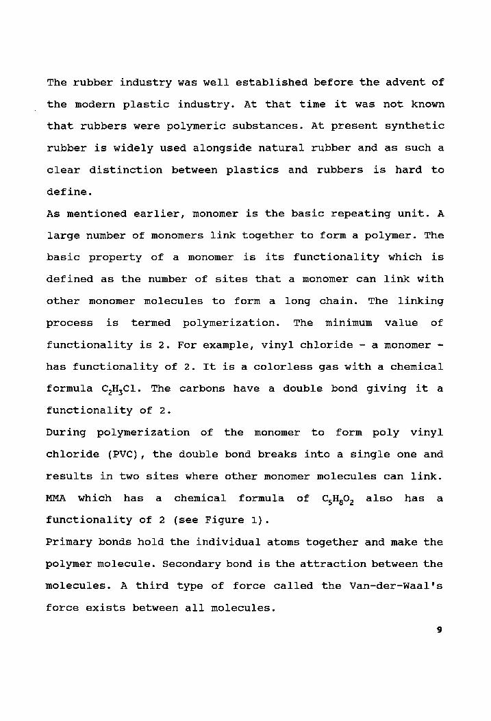
MMA which has a chemical formula of C,H,O, also has a

functionality of 2 (see Figure 1).

Primary bonds hold the individual atoms together and make the

polymer molecule. Secondary bond is the attraction between the

molecules. A third type of force called the Van-der-Waal's

force exists between all molecules.

ah on!

° H—-C-H

Figure 1 Chemical Structure of MMA

Bond length is the distance between the individual carbon

atoms. Bond energy is the external energy required to break

the bonds between carbon atoms, expressed as the amount of

energy per molecule. Both these quantities are constant for a

particular type of bond. As an illustration, a double bond has

a bond length of 1.32 x 10°'° meter and possess a bond energy

of 607 kJ/mol. As can be expected, a triple bond has a shorter

bond length and a larger bond energy. Another parameter of the

structure is the bond angle, which is the angle between

individual carbon atoms. This quantity is also constant for a

specified type of bond. A single bond molecule is free to

rotate about the C-C bond while the double and triple bond

molecules can experience no rotation.

A polymer can form in linear chains of monomer or it can be a

branched chain. A third possibility arises when there are two

or more kinds of repeating units. This type of polymer is

called a copolymer. Depending on the relative position of its

constituting repeating units, a copolymer can be further

divided into alternating copolymer, random copolymer and the

block copolymer.

A polymer can also consist of two and three dimensional

networks of chemical bonds. Graphite has a two dimensional

network while diamond is three dimensional. The networks are

interconnected through primary chemical bonds and are called

cross linked polymers. Cross linking increases the mechanical

11

strength of a polymer.

Converting the monomer into polymer, that is the process of

polymerization can occur in three ways depending upon the

monomer involved. They are chain polymerization, stepwise

polymerization and thermoset polymerization. In chain

polymerization a single monomer continues to link with the

same repeating unit until a stable configuration is reached.

There are very few intermediate polymers formed. In stepwise

polymerization, the polymerization occurs ina number of steps

with intermediate polymers formed at each stage of its

formation. Thermoset polymerization occurs when there are more

than two functional groups in a step polymerization reaction.

The reaction leads to branched structures which intercombine

to random three-dimensional networks which finally extends

through the whole mass to form a single giant molecule. The

degree of polymerization is defined as the weight of a typical

polymer molecule divided by the weight of the repeating unit.

12

2.2 Polymers in Bridge Deck

The main reasons for the growing use of polymers in bridge

deck repair and rehabilitation are its properties of rapid

cure and low permeability as well as the flexibility of many

possible formulations. It has been estimated that about 90% of

the voids in concrete is filled up by the process of polymer

impregnation.

The factors which control the selection of an appropriate

monomer system are familiarity with its physical, chemical,

fire hazard and health hazard properties. In an earlier study

on the use of polymers in highways [9], the monomer system

chosen was one for which all of the aforementioned properties

were known in detail. The system was as follows:

90% Methyl Methacrylate (MMA)

10% Trimethylolpropene trimethacrylate (TMPTMA)

0.5% of the above monomer mix of Azobisiobutyronitrile (Azo)

All the above proportions are by weight. TMPTMA is the cross

linking agent. The Azo acts as the initiator to the

polymerization reactions.

In the present study, the same monomer system was employed.

Other monomer system can conceivably be used once detailed

knowledge of its properties is available.

The specific advantages of this monomer system are mainly its

properties of low viscosity and its rapid auto accelerating

13

polymerization reaction.

However, this monomer system has several disadvantages, most

of which can be virtually eliminated by adhering to good

safety practices. They are flammability (due to its low flash

point at 70° F and high vapor pressure), high cost, toxicity

and its irritating odor.

Standard precautionary measures employed during the handling

of the monomer were as follows:

(1) The three components of the monomer system were stored

separately in adequately ventilated areas with explosion proof

electrical facilities.

(2) Mixing was done under the fume hood at a temperature not

exceeding 70° F. Over this temperature, the components may

react spontaneously giving rise to an exothermic reaction.

(3) Care was taken not to subject the Azo to strong physical

shocks.

(4) The Azo was refrigerated when not in use due to

flammability at high temperatures.

(5) The maximum volume of monomer mixed in one batch was

allowed not to exceed 55 gallons.

(6) All unused monomer mixture was kept under refrigeration

and later disposed of safely by burning.

(7) Monomer loading was initiated only after the concrete had

cooled to a temperature below 100° F.

(8) Class B fire extinguishers were kept available.

14

(9) During impregnation all persons in the immediate vicinity

wore protective gloves, masks and goggles.

15

3.0 REVIEW OF CORROSION

3.1 Mechanism of Corrosion

The process of corrosion involves the conversion of metal into

non-metallic corrosion products. When the metal involved is

iron or its products like steel, the phenomenon is called

rusting and the non-metallic end product is called rust [10].

Although the only metal considered in this study is steel (the

reinforcing bars in concrete bridge decks), the more general

term "corrosion" will be used throughout. Pore water in

reinforced concrete is alkaline in nature with a pH value

between 12.5 and 13.5 [11,12]. A layer of gamma iron oxide

(Fe,0,) is formed around the steel in this alkaline environment

which renders it passive thus preventing the onset of any

corrosion activity. Thus, the breaking down of this passive

layer by any external agent will cause corrosion to initiate.

The passive layer can be degraded primarily by two mechanisms.

One is by leaching of water or a reaction with carbon dioxide

or other acidic material which causes partial neutralization

of the passive layer. Depassivation will occur if the pH value

drops below approximately 10-11 [13]. The second mechanism is

by electrochemical reactions involving chloride ions in the

presence of oxygen. Relative to corrosion in bridge decks, the

16

latter is by far the predominant method in which the passive

layer is destroyed.

As mentioned earlier, the major source of chlorides on bridge

decks is from the deicing salts - mainly sodium and calcium

chloride - used during the winter season. Splashes and sprays

from sea water on concrete bridge components in marine

environment is a second source. Chlorides may also be present

in the mixing water, in admixtures (if used) or in aggregates

in the concrete mix.

Chlorides penetrate into the concrete mainly by the process of

diffusion. Another mode is through cracks on the deck which

may have been formed due to shrinkage or other means. When the

chloride ion concentration at the rebar level reaches the

threshold level, the corrosion reactions start. From previous

studies, the level is taken as 1.2 lb of chloride ions per

cubic yard of concrete [14].

The chloride ions which first react with iron are then

released for reuse; thus an accumulation of chloride ions are

maintained. The corrosion product, rust has a larger volume

than steel. The generated pressure causes a rupture in the

concrete above the surface of the rebar. The cracks which are

formed allows an increased penetration of chloride and oxygen

which in turn accelerates the corrosion rate.

17

The electrochemical reactions in chloride contaminated

concrete are as follows.

Anode Reactions:

Fe + 2Cl° > Fe** + Cl’ + 2e

Fe"Cl, + 2H,O > Fe(OH), + 2H* + 2Cl°

In the presence of oxygen:

6(Fe** + 2Cl) + 0, + 6H,O > 2Fe,0, + 12H* + 12C1°

Cathode Reaction:

40, + HO + 2e° > 20H

A corrosion cell consists of two electrodes, the anode and the

cathode, which are electrically connected so that electrons

can flow. In concrete the reinforcing steel is the electrodes

and the medium through which the current is propagated is the

pore water.

The Electromotive force (EMF) of a cell is the algebraic sum

of the two electrode potentials. As a reminder, electrical

potentials are normally stated in comparison to the potential

of the hydrogen electrode. As the electrode with the lower

potential value will undergo corrosion, the EMF of a cell is

always negative. It follows that the more negative the EMF is,

the greater the corrosion activity. If there is no difference

18

in potential between the cathode and anode, the EMF of the

cell is zero and there is no flow of current and no corrosion

activity.

In the corrosion reactions, the anode undergoes oxidation and

is the electron donor as has already been illustrated in the

reactions listed in page 18. The cathode undergoes reduction

and is the electron acceptor. Thus, the corroding site is the

anode.

Faradays' first and second law govern the rate of corrosion.

The first law states that the rate of corrosion is directly

proportional to the corrosion current. In mathematical terms:

weight of metal reacting/time a I corr

or R=kKI (1) corr

where,

R = rate of corrosion in grams/second,

k electrochemical equivalent in grams/Coulomb, and

Lior = Corrosion current in Ampere.

The second law of Faraday states that the rate of reaction at

the anode is equal to the rate of reaction at the cathode.

For bridge decks, cracking is a secondary mode of entry of

chloride ions, the primary mode being diffusion. Cracks may

occur due to load deflection during concrete placement

operation, plastic shrinkage, drying shrinkage or by

subsidence cracking. Subsidence cracking occurs due to the

19

differential settlement of concrete. If t, is the tensile

stress due to the differential settlement of concrete and t,

is the tensile strength of the fresh concrete, subsidence

cracking will take place if

t, > t,

A possible third mode of chloride penetration was thought to

be by capillary action. However this has been discarded as

being extremely doubtful [14]. Capillary action is thought to

be prevalent to a depth of about 0.5 inch or 1.27 cm from the

top surface of the bridge deck.

The process of diffusion of chlorides through concrete obeys

Fick's second law.

§c/ét = D, (6*C/ 5X?) (2)

where,

Cc chloride ion concentration in %,

= distance or depth in cn, Xx

t time in years, and

D. = diffusion constant in cm*/year.

20

A solution to the above second order differential equation is:

C(X,t) = C, [1 - erf{X/(2 v(D,t))}]

where,

Cc, = integration constant in %, and

erf is a probability function based on random variable.

Desired values are available from standard tables.

As the chlorides penetrates into the deck from the top

surface, the top mat of rebars which it would encounter first

will be the corroding site and act as the anode.

There are two types of corrosion cells. Micro~cell corrosion

occurs when the cathode and anode are close to each other as

on the same rebar in a bridge deck. In macro-cell corrosion,

the cathode and anode are separated by some distance. In a

bridge deck, the anode will be located in the top mat of

rebars while the cathode will be in the bottom mat of rebars.

It has been estimated that 90% of bridge deck corrosion is

micro-cell in nature.

21

3.2 Factors Influencing Corrosion

Corrosion of steel is influenced by various factors like cover

depth, type of cement, relative humidity, nature of ions

present, concrete permeability or its indicator water/cement

(w/c) ratio and degree of consolidation.

The presence of oxygen is an important factor in initiating

the corrosion reaction. However, in most cases oxygen is

readily available for diffusion into the concrete. A far more

important factor is the water content of the concrete. Ata

low water content there is very little ionic conduction and

the corrosion rate is low. At very high water contents there

is less available oxygen and the corrosion rate is low. Thus,

there is an optimum water content at which corrosion is least

inhibited [15]. As with lower permeabilities, larger cover

depths increase the time to initiate corrosion. Whereas a

lower permeability decreases the rate of chloride diffusion,

larger cover depths increase chloride diffusion path length.

22

4.0 EXPERIMENTAL DESIGN

4.1 Overview of Experimental Design

Simulation of bridge deck conditions was achieved in the

laboratory by casting small reinforced concrete specimens.

Previous studies had indicated that scaling down test

specimens from bridge deck size to laboratory size has no

substantial effect on the validity of results obtained and

results and conclusions from one apply equally to the other.

Eighteen specimens of approximately one foot-square were made

with two triad of rebars in each specimen. The specimens were

then subjected to alternate wet and dry cycles with salt

solution until corrosion had been initiated. The 3LP device

manufactured by Kenneth C. Clear, Inc. as well as standard

copper-copper sulfate half cell (CSE) were used to determine

the degree of corrosion activity in the specimens. These

measurements were further validated by determining the

chloride ion concentration of the concrete. Once it was

evident that there was active corrosion in the rebars, the

specimens were subjected to five different corrosion abating

treatments. Treatments included LMC and LSDC overlays and

impregnation with the chosen monomer system. Control specimens

were not treated. A comparison of pre and post treatment

23

corrosion activity for each treatment method indicated the

effectiveness of the treatment procedures as a means of

arresting corrosion in bridge decks.

In the study just outlined, the concrete was dried prior to

impregnation such that the temperature at half inch below the

top rebar was about 230 °F. This is the drying criterion used

in previous polymer impregnation studies [9]. However, if a

lower drying temperature was to be equally acceptable for

effective impregnation, it would represent a large saving of

time, energy and consequently cost. In order to investigate

that possibility, a number of mortar cubes were made. They

were divided into several sets and each set was dried to a

different temperature ranging from room temperature to 600 °F.

The cubes were then polymer impregnated. Cut pieces of the

cubes were evaluated using a mercury porosimeter and a

scanning electron microscope. The cubes were also exposed to

saline environment and chloride content tests were run to

obtain the resistance of polymer impregnation following

different degrees of drying to the ingress of chloride ions.

Results obtained from these studies indicated that a lower

drying temperature was sufficient for the purpose of

impregnation.

To validate the above conclusion, several other laboratory

specimens were dried to 150 °F and 180 °F (temperature at half

inch below the top rebar level) and then polymer impregnated

24

as before.

25

4.2 Impreqnation of Rigid Overlay Systems

In the past, deep polymer impregnation (impregnation to a

depth of 3" to 4") had been used as a rehabilitation technique

for salt contaminated but sound bridges. With the development

of the grooving procedure, [6,7] deep polymer impregnation

became feasible under other conditions such as decks with

rigid overlays where the sound but chloride contaminated

concrete had been left in place.

The objective of this study was to evaluate polymer

impregnation of overlaid bridge decks as an effective means of

abating corrosion. AS a means for comparison, several

treatment methods were employed other than impregnation

through rigid overlays.

Eighteen laboratory concrete specimens were cast. They were

12" long and 10 %" wide. Each specimen had two triad of

rebars, see Figure 2. Each triad consisted of one rebar at the

top and two rebars equidistant from the top rebar at the

bottom, thus forming an isosceles triangle. The bottom rebars

were 1 \" from the bottom of the specimens. The rebars were

placed along the width of the specimens. The rebars were

approximately 11 %" long such that they extended about %" each

beyond the two ends of the specimens. The rebars used were #4

(ASTM specifications A 615) with nominal diameter of 4%". The

overall height of the specimens was 4". The cover depth was

26

12.0°

ea aeweoe

ee ee

' ‘ ‘ ‘ ’ ‘ ‘ ’ i ‘

+ ’ $ ‘ ’ a ‘ ’ ' 4 ' ' ' ' ‘ ‘ ‘ ‘ ‘ ‘ ‘ ‘ ‘ i

4 ‘ i '

t ' ' ‘ 1 ‘ i ; ‘ ‘ ‘ ‘ ‘ ‘ ‘ ‘ ‘ 1 ‘ ‘ ’ ’ ‘ ' ’ ’

' ,

o ‘ , 4 ’ ‘

10.376°

“ek O

Figure 2 Plan and Elevation of Specimens

27

1".

The forms for the specimens were made of %" plywood A-C

exterior grade and fastened by 2" #8 dry wall screws. Spacers

of dimensions 4%" x \" made of plexiglass were used on one side

of the forms (two spacers per form) so that the thermocouple

(TC) wire could be accommodated. For adequate clearance, holes

that were drilled in the form for the rebars were %" in

diameter.

The rebars were cut to size, drilled and tapped at one end to

a depth of %" to accommodate screws of diameter ‘%". In order

to minimize the effects of manufacturing oil and existing rust

on the rebars, the rebars were cleaned by soaking ina

solution of hexane for about 20 minutes and then wiped clean.

The rebars were then dried in an oven at 240 °F for 10

minutes. Hexane is a suitable cleanser as it leaves no

residual ions on the rebars and thus eliminates contamination

from the cleaning process. To prevent corrosion from taking

place at the exposed ends, the two ends were covered by

electroplating tape such that the uncovered length of each

rebar was 6.5". Thus the exact surface area exposed for

corrosion was known and hence corrosion rates could be

normalized to a square foot of surface area of the rebar. The

wooden forms were painted with two coats of form oil with

overnight drying between coats. This was done to prevent the

concrete from adhering to the forms.

28

Thermocouple (TC) junction was taped at the center of each top

right rebar of the specimens. Type T plugs were attached to

the other ends. The TC was thus designed to indicate

temperature at the top rebar, i.e. the anode of each specimen.

A notch was filed at the bottom of the hole in the forms which

would contain the TC attached rebar to facilitate pulling out

of the TC wire out of the hole after the specimens were cast.

The rebars along with the TC wire and spacers were assembled

in each form in an inverted configuration to minimize

consolidation (subsidence) cracking. Care was taken to ensure

that the drilled and tapped holes in all rebars were on the

same side. The forms were then codified with a permanent

marker according to the treatment process each specimen would

undergo. Five treatment methods were used and one set of

specimens acted as controls which were not subjected to any

treatment. Thus there were six sets of three specimens each.

The two letter code assigned to each set was as follows:

ecO: Specimens which acted as controls and were not treated,

eLM: Specimens which were overlaid with LMC,

eLS: Specimens which were overlaid with LSDC,

ePC: Specimens which were polymer impregnated,

ePM: Specimens which were overlaid with LMC and

polymer impregnated, and

ePS: Specimens which were overlaid with LSDC and

polymer impregnated.

29

To distinguish between the three specimens in each group,

numbers 1, 2 and 3 were used after the two letter code. For

instance, the three specimens which were polymer impregnated

were named PCl1, PC2 and PC3.

Concrete was then placed in the forms. For mix designs,

properties and compressive strengths see Appendix A. The

specimens were removed from their forms after 24 hours of

moist curing. Being cast inverted, the top surface of the

specimens were in contact with the wooden form. There was a

possibility of the surface being contaminated with form oil.

To eliminate this, the surfaces were cleaned with muriatic

acid (dilute hydrochloric acid).

In bridge decks, there is no ingress of salt from the sides.

To incorporate this factor into the laboratory specimens the

Sides were coated with epoxy. Two kinds of epoxy were used for

this purpose. The first was EP-5. This epoxy consists of two

components, A and B which were mixed in equal proportions for

three minutes with a paddle attached to a hand drill. The

other type of epoxy was Epon 828 resin. 100 parts of the resin

was mixed to 10 parts of DETA (the curing agent) by weight.

These epoxies have relatively short curing time and small

batches were mixed at one time to prevent premature hardening.

Care was taken to ensure that no epoxy spilled on the top

surface or seeped to the bottom surface.

Plexiglass dikes 1" high and 5/16" thick were fixed on top of

30

each specimen with silicon rubber. Glass covers were used on

the specimens to minimize moisture loss during wet cycles.

Electrical connections were fitted on the rebars with screws

of diameter %". A resistor of 100 N was connected between the

top rebar and bottom right rebar of each triad. A jumper cable

was fitted between the two bottom rebars of each triad.

Prior to the first wet cycle, potential and temperature

readings were taken in order to establish base readings.

Temperature readings were with a digital Type T TC meter.

Potential readings were taken with a CSE half cell according

to the procedure outlined in ASTM C-876 [16]. For each top

rebar, three readings were taken one in the front, one in the

middle and one in the rear of the specimen. The three readings

for each rebar did not show appreciable variation and the mean

of the three readings was recorded. The interpretation of the

potential values are also given in ASTM C~876 and are:

eIf the potential is more positive than -200 mV CSE, there is

a probability of more than 90% that there is no active

corrosion present.

elf the potential is between -200 mV CSE and -350 mV CSE,

corrosion activity is in the uncertain region.

elf the potential is more negative than -350 mV CSE, there is

a probability of more than 90% that there is active corrosion

present.

31

Thus, the interpretation of the potential values from the

copper-copper sulfate half cell is based on a probability

function.

Five days after the concrete was placed, the first wet cycle

was started. As the permeability of concrete decreases with

age, the first wet cycle was started as soon as practicable to

introduce chloride ions into the concrete at the earliest. A

6% solution of sodium chloride by weight was used as the

source of chloride ions for the concrete. 500 ml of the

solution was used for ponding each specimen. The wet cycle

extended for a period of three days. At the end of the period,

the solution was taken off the specimens with a 2.25 peak HP,

16 gallon wet-dry shop vacuum. During the dry cycle the

ambient temperature was raised to 120 °F by using several

infra red lamps. The maximum temperature that the concrete

attained at the top rebar level was in general somewhat higher

than the highest ambient temperature. The high temperature

dried the concrete and made it moisture hungry so that the

penetration of salt solution during the next wet cycle was at

a higher rate. The duration of the dry cycle was four days.

Ponding with salt solution was continued and measurements were

taken periodically.

Another instrument, the three electrode linear polarization

device (3LP device) manufactured by Kenneth C. Clear, Inc. was

used to monitor the corrosion current. As mentioned in the

32

previous chapter, the corrosion rate of metal is directly

proportional to the corrosion current. The 3LP devise

impresses a current in the reverse direction and polarizes the

corrosion current. Knowing the impressed current and the

corresponding value of the potential, the corrosion current is

obtained by using the Stern-Geary equation. A description of

the test procedure is outlined in Appendix B. Interpretation

of the corrosion current (I...) values obtained is given in corr

the 3LP manual [17] as:

elon < 0-2 mA/sq ft > no corrosion damage expected.

elo. between 0.2 and 1.0 mA/sq ft ~ corrosion damage possible

in 10 to 15 years.

elo, between 1.0 and 10 mA/sq ft > corrosion damage expected

in 2 to 10 years.

eliorr 7 10 mA/sq ft > corrosion damage expected in 2 years or

less.

During the ponding period, chloride contents of some selected

specimens were determined at different depths using the

specific ion probe test method developed by James Instruments,

Inc. [18]. Description of the method can be found in Appendix

B. Earlier work by Herald [19] correlated the results

obtained by the specific ion probe method and the standard

AASHTO test method, T-260-78.

In the available literature, several different values of

chloride ion concentration have been suggested as a threshold

33

value for the initiation of corrosion. The author has used the

value of 1.2 1b of chloride ions per cubic yard of concrete as

concluded from research done by the Federal Highway

Administration (FHWA) [20,21].

The alternate wet and dry cycles were continued and corrosion

activity was monitored at regular intervals.

Treatment activities were started when it was determined that

there were active corrosion in most of the rebars. At that

point in time, all the potentials were more negative than 350

mV, the mean corrosion current was 4.2 mA/sq ft with most of

the values being over 2 mA/sq ft and the chloride content at

the rebar level of selected test specimens were greater than

1.2 lb/cubic yard. The treatments took about a month to be

completed from the time the last pre-treatment measurements

were taken. Several sets of readings prior to treatments

indicated accelerating rates of corrosion in the rebars. Thus,

it is likely that the corrosion levels were higher when the

treatments were applied than were indicated in the last pre-

treatment readings.

During the treatment processes, the application of periodic

salt solution on all the eighteen specimens were suspended.

As a reminder, the specimens of the LM and LS series were

overlaid by LMC and LSDC, respectively. The PC series was

polymer impregnated. The PM series was overlaid with LMC and

polymer impregnated while the PS series was overlaid with

34

LSDC and polymer impregnated. The CO series were left

untreated. Thus, there were twelve overlayed specimens, nine

impregnated specimens and three untreated specimens.

Twelve forms with height measuring about 6" were made to

accommodate the overlays which were 2" high. As before, two

coats of form oil were applied to the forms. The specimens of

the LM, LS, PM and PS series were placed in the form. The

inner periphery between the edge of the specimens and the form

was covered by duct tape to prevent the overlay concrete from

dripping along the sides of the existing concrete. The

surfaces of the specimens were wetted with plain water and

covered with plastic sheets twelve hours prior to the

application of the overlays.

LMC overlays were applied to the LM and PM series, while the

LS and PS series were overlaid with LSDC. Mix designs for LMC

and LSDC, properties of the aggregates and compressive

strengths of the overlays are given in Appendix A.

The specimens with LMC overlays were kept moist for 48 hours

while the specimens with LSDC overlays were kept moist for a

period of 14 days. This was done by placing moist burlap

covered by plastic sheets on the specimens and keeping the

burlap wet during the period of moist curing. After the curing

period, the specimens were freed of the forms. The sides of

the overlays were coated with epoxy like the original concrete

layer.

35

The seven and fourteen day compressive strengths of the

overlays were satisfactorily high for the next step of the

treatment procedures for the overlayed specimens to be

initiated.

The specimens of the PC, PM and PS series had to be grooved as

the first stage in the polymer impregnation treatment process.

In an earlier study [7], an empirical formula was developed to

determine the grooving parameters: groove spacing, groove

depth and groove width for optimum polymer impregnation. The

objective in deep polymer impregnation is to encapsulate the

steel by impregnating the concrete to about a depth of 4"

below the top rebar level. A greater depth is not desired as

impregnating the concrete further is redundant and the larger

volume of monomer required becomes an unnecessary expense.

Encapsulation of the top rebar results in isolating the anode

and thus forcing electrical discontinuity between the cathode

and anode. Consequently, the corrosion current decreases.

In this study the grooving parameters were roughly determined

by assuming a 10% polymer loading of concrete by volume as

determined in the earlier study [6,7]. The depth of

impregnation is %" below the top rebar.

There were two values of depth of impregnation involved. The

specimens of the PC series had the original cover depth of 1"

and the final depth of polymer penetration was 2". For these

specimens, the depth of groove was 4%". For all the specimens,

36

the groove width was %" and the edge to edge distance between

grooves was 2 4". The overlay specimens (PM and PS series) had

a cover depth of 3" and the final depth of polymer penetration

was to be 4", The groove depth for the overlaid specimens was

2 4". With the above groove parameters, the number of grooves

on each specimen was three (see Figure 3).

The groove lines were marked on each specimen with a permanent

ink marker. A masonry saw was used to cut along the groove

lines. Concrete between the cut lines were then chipped out

with a mason's chisel.

The next stage in treatment for the three impregnated series

(PC, PM, PS) was drying. Prior to monomer impregnation, the

concrete has to be sufficiently dry so that the monomer can

diffuse into the concrete and fill the void spaces. Thus, it

would seem that the concrete had to be dried to above the

boiling point of water at the depth of impregnation which is

+" below the top rebar level. The drying temperature used at

this depth in a former study on polymer impregnation of

concrete [9] was 230° F. The same value was used in the

treatment of the current specimens. Later studies investigated

the possibility of using lower drying temperatures without

lower corrosion abatement effectiveness (see section 4.3).

Because concrete bridge decks have to be dried from their top

surface, oven drying was not appropriate. Thus, propane fired

infra-red heaters were used to dry the specimens. Three

37

Q

OD = 1/2" for PC

Mm = 2 4/2" tor PM and ?S

Figure 3 Groove Dimensions

38

heaters were placed side by side suspended by chains from a

metal framework so that the height of heaters from the top of

the specimens could be adjusted as necessary. A partial

enclosure was made around the heaters to a height of 3 feet

from ground level with sheet metal. The pressure of the gas

was adjusted to 3 psi.

In order to monitor the temperature at a depth of 4" below the

top rebar level high temperature TC wires were encased in

ceramic tubing and inserted into a hole made in the bottom of

the specimens to a depth such that the TC junction was 4"

below the top rebar. A 4%" carbide drill bit was used to drill

the TC holes. The TC wire inside the concrete was kept secure

in the concrete by duct tape. The TC wire used was about five

feet in length so that the other end could be brought out of

the drying enclosure.

The nine specimens were set up below the heaters. For

uniformity, all the specimens were placed so that their top

surfaces were at the same level and thus all the specimens

were at the same distance from the heaters. Fiberglass

insulation (3%" thick) was wrapped around the specimens. The

fiberglass was supported by a layer of sand and gravel. The TC

wires leading outside the enclosure were covered with sand and

gravel. Insulating the specimens thus, prevented the entry of

heat from the sides. The TC wires were insulated so that the

TC junction would measure the temperature at the proper

39

location. A metal sheet with rectangular holes cut in it was

placed over the specimens so that only the top of the

specimens was exposed to the heaters. This ensured that the

concrete was heated only from the top surface.

Along with the nine specimens, three 4 x 8 cylinders made from

the same concrete mix design as the impregnated specimens were

also dried. The cylinders were used to determine the rate of

monomer impregnation of the concrete.

A tag was attached to each TC wire to identify each specimen

when the temperatures were taken during the heating and the

subsequent cooling. A probe was fixed to record the shaded

ambient temperature outside the heating enclosure. A second

probe was placed on the top surface of the specimen at the

center of the drying area in order to record the surface

temperature.

The heaters were then lowered so that the distance between the

edge of the heaters and the top surface of the specimens was

9",

Initial temperatures were taken of all locations before the

heaters were turned on. The locations were internal

temperatures at %" below the top rebar level, surface and

ambient temperature.

The heaters were then turned on with a self-igniting propane

fired torch. Temperatures at all locations were recorded at

regular intervals.

40

After 70 minutes of heating, the internal temperatures of two

specimens, PCl and PC3 reached 230° F. As the internal

temperatures of the other specimens were substantially lower,

the heaters could not be turned off. To remedy the situation,

the two specimens were covered with a metal sheet to prevent

further heating of these specimens.

At 150 minutes, most of the specimens had internal

temperatures which were nearly the requisite value. Therefore,

the heaters were turned off. Because concrete acts as a heat

sink, the internal temperatures of all the specimens continued

to rise even after the heaters were turned off until a thermal

equilibrium was established. Thus, the maximum internal

temperatures of all but two specimens were in the vicinity of

230 °F.

Temperatures at all the previous locations were taken at

regular intervals after the heaters were turned off.

Temperature readings were taken for about five hours after the

heaters were turned off. The specimens were then covered with

a layer of fiberglass insulation and left to cool for about 12

hours before impregnation was started.

The ends of the grooves in the nine specimens were sealed with

epoxy putty which does not dissolve in MMA. Like most epoxies,

epoxy putty has two components which were mixed in equal

quantities by kneading vigorously by hand. After application,

the epoxy putty was allowed to cure for about two hours. The

41

putty was also used to make dikes about one inch high on the

three cylinders. The specimens and the cylinders were covered

with plastic sheet cut to size and taped around the edges with

duct tape. A slit was made in the middle of the plastic of

each. The slits were covered by pieces of duct tape. This

arrangement ensured little loss of the monomer by evaporation

during the monomer loading period.

The monomer was mixed carefully under the fume hood. 90 % of

MMA was mixed with 10 % of TMPTMA, by weight. 0.5 % of the

above mixture of Azo, by weight, was added.

The monomer was ponded on the top surface of the specimens and

cylinders using a 20 ml pipette and placed through the slit in

the plastic. The slit was kept covered after monomer was

placed on the specimens.

The three cylinders which were marked as 3E, 6E and 7E had

impregnation times of 6 hours, 14 hours and 23 hours,

respectively. During this period more monomer was added as

required when all existing monomer had diffused into the

concrete. The same was done in the case of the specimens

during their impregnation period. After the designated

impregnation time for each cylinder, the residual monomer was

drawn off with the pipette. Volume of monomer placed on each

cylinder as well as the volume of the remaining monomer at the

end of the impregnation periods were recorded.

The cylinders were then placed in a hot water bath at 185 °F

42

for polymerization of the monomer. They were kept in the bath

for four hours. The cylinders were taken out of the bath and

cut longitudinally in half using a masonry saw. The cut

cylinders were then etched with muriatic acid. The acid etches

all portions of the concrete except the area of impregnation.

Thus, the depth of impregnation of the cylinders could be

visually distinguished. A previous study [9] demonstrated that

the rate of monomer impregnation of concrete is a function of

the square root of time of impregnation.

Using this relation a graph of depth in inches versus square

root of time in hours was plotted from the data obtained from

the acid etching of the three cylinders. A fourth data point

was the origin of the graph. The resulting graph was a

straight line (see Appendix C). Thus, the rate of impregnation

for the particular concrete was ascertained. As the bottom of

the grooves in the specimens were 4%" above the top rebar level

and the desired depth of impregnation was %" below the top

rebar level, the distance monomer had to diffuse in the

specimens was 1". Since the monomer loading is approximately

10 % by volume, the actual depth of impregnation was 1.5 + 0.9

= 1.67". From the graph, the time corresponding to this depth

is 16 hours.

Accordingly, the specimens were allowed to be impregnated for

a period of 16 hours. At the end of this period, the residual

monomer was drawn of with a pipette and the specimens were

43

polymerized in a water bath at 185 °F for 24 hours. During

this period the specimens also absorb water.

At the end of 24 hours, the heaters were turned off and the

specimens taken out. The grooves in the PM and PS series of

specimens were filled with latex modified mortar (LMM). For

mix proportions of the LMM, see Appendix A.

Application of salt solution was resumed with the same wet and

dry cycles used before treatments.

Post treatment potential and corrosion current measurements

were taken periodically.

Potential and I,,,. readings were also taken with different

cathode to anode surface areas (C/A). In the standard

electrical connection on the specimens, the C/A surface area

ratio was 2. C/A ratios of 1, 3 and 4 were achieved by

isolating the left anode, and connecting jumper cables such

that the right anode was connected to 1, 3 and 4 cathodes

(bottom rebars), respectively. As the left anode had been

isolated, micro-cell corrosion readings were taken on this

rebar.

This study was done to investigate the effect of C/A surface

area ratio on the corrosion rates and to compare micro-cell

corrosion to macro-cell and mixed-cell (combination of micro

and macro) corrosion rates.

Along with the mixed-cell corrosion readings, the macro-cell

corrosion readings were also taken. This was done by

44

connecting a volt meter across the resistor and recording the

potential drop in mV. Since the value of the resistor was 100

Nn in each case, the corresponding macro-cell current was

obtained in mA using Ohms Law. (Current = Potential/Resistance)

45

4.3 Optimizing the Drying Temperature for Corrosion Abatement

4.3.1 Effects of Drying Temperature on Corrosion Properties

As mentioned in the preceding section, the drying temperature

of the concrete at a depth of 4%" below the top rebar level

prior to monomer loading was 230 °F. This value was used ina

previous study [9] on polymer impregnation of concrete. The

objective of this study was to investigate the possibility of

using a lower drying temperature which would reduce drying

time and substantially reduce impregnation costs. Specially,

for a long bridge deck this would translate into a

considerable reduction of time and money.

It was decided that the influence of the drying temperature on

the corrosion properties would be studied for a wide range of

temperatures.

Forty-two 2" mortar cubes were made for this experiment. For

mix proportions, and other properties, see Appendix A. The

cubes were made in accordance with ASTM C-109-90. The cubes

were divided into 14 sets each set containing three cubes.

The cubes were taken out of their molds after 24 hours and

inscribed with codes with a permanent ink marker. The codes

used for the sets were the numbers 1 through 13 and the

letters 'CON', standing for control specimens. The cubes in

each set were marked with letters A, B and C. The cubes were

46

then moist cured for thirty days.

After curing the cubes were air dried. The cubes in set 1,

that is cubes 1A, 1B and 1C were tested for compressive

strength. The results are presented in Appendix A.

The cubes in set 2 were air dried at room temperature (75° F).

The cubes in set 3 through 13 were oven dried to the following

temperatures: 100 °F, 125 °F, 150 °F, 175 °F, 200 °F, 225 °F,

250 °F, 300 °F, 400 °F, 500 °F and 600 °F.

The cubes were weighed once in each 24 hour period to the

nearest 1/10th of a gram using a digital scale. The weights of

the cubes before the drying stage were approximately in the

range 270 g to 290 g. Each set of cubes were taken to be fully

dried to its designated drying temperature, when the decrease

in the weight of each cube was less than 0.1 % of its weight

in a 24 hour period, that is the difference in weight was

roughly less than 0.3 g in each 24 hour period. All the cubes

were placed in the oven at one time and the oven set to the

lowest drying temperature: 100 °F. When the cubes of set 3

were completely dry at this temperature, they were taken out

and placed in a desiccator to prevent any absorption of

moisture before the cubes could be impregnated. The oven was

then set at the next higher temperature, 125 °F and so on

until all the cubes were dried.

At lower temperatures, the cubes required a relatively longer

time to be dry. As the drying temperature at this point was

47

less than the boiling point of water, the molecules of water

took a long time to evaporate from the cubes. For the cubes

that were dried at temperatures below 225 °F, it took between

7 to 11 days to dry. In the case of cubes over this

temperature it progressively required a shorter time as the

drying temperature was increased. For the last set of cubes,

it took 48 hours from the time the penultimate set of cubes

were removed and the oven temperature raised to 600 °F.

As mentioned before, the dried cubes were placed in a

desiccator before impregnation could be initiated. The drying

agent used was anhydrous CaSO, which is a deliquescent

material and absorbs water vapor from the atmosphere. Two

kinds of CaSO, granules were used: a non-indicating and

relatively cheap white colored type and an indicating but more

expensive blue colored type. A handful of the blue type was

mixed with a larger quantity of the white type in the

desiccator. On absorbing water molecules, the blue granules

turn to a purple color.

The desiccator lid was sealed using vacuum grease.

Monomer was mixed in a Similar way as in the case of the

specimens described in the preceding section. The cubes were

again weighed and then impregnated by submerging them in

monomer inside a metal box for a period of five days. During

the impregnation period, care was taken so that the cubes were

completely submerged at all times.

48

After the impregnation period, the cubes were taken out of the

box and allowed to be air dried. Another set of weights were

then taken.

The cubes of set 2, that is the cubes which were dried to

ambient temperature, showed random cracks all over the

surfaces. One cube had a small piece which had completely

broken off. The other cubes which were dried to higher

temperatures did not appear to be cracked. An earlier

experiment performed on mortar cubes by the author resulted in

the cubes dried to ambient temperature cracking during the

impregnating stage. Repeatability of this phenomenon precluded

faulty mix design as being a possible cause of the cracks.

This matter is discussed further in Chapter 5.

Each cube was individually wrapped in aluminum foil and each

set of cubes were placed in water proof plastic bags and

immersed in a water bath at 185 °F for 24 hours. The aluminum

foil and plastic bag were used to prevent the cubes from

absorbing water during polymerization, so that when they were

vacuum saturated the moisture content would be due to water

uptake during the vacuum saturation only.

After polymerization, the cubes were removed from the bath,

allowed to cool to ambient temperature and another set of

weights were taken.

The cubes were then vacuum saturated, and the moisture content

of the cubes were determined as follows:

49

Moisture Content = {(W)/W,) x 100} %

where,

W ‘ weight of water absorbed in vacuum saturation in g, and

W 5 weight of the cube before vacuum saturation in g.

The resistivity of the cubes were obtained by using a Nilsson

Soil Resistance Meter [22]. For the purpose, the instrument

was modified slightly. See Appendix B for a description of the

testing procedure.

Three resistivity values were taken across each pair of

opposite sides of the cubes for total of nine values from each

set of three cubes. The mean value of the nine resistivity

readings was used for analysis.

The suggested criteria used for interpreting the resistivity

values is presented below [23,24].

elf resistivity exceeds 12,000 N-cm, corrosion is unlikely.

elf resistivity is between 5,000 N-cm and 12,000 N-cn,

corrosion is probable.

elf resistivity is less than 5,000 N-cm, corrosion is almost

certain.

A separate study on marine structures in California indicated

that at resistivity values over 60,000 N-cm no corrosion

occurred but corrosion was detected below 60,000 N-cm [25].

Other work [26] suggested that corrosion was unlikely above

50

20,000 N-cm and active corrosion would occur at resistivities

between 5,000 to 10,000 Q-cm.

A masonry saw was used to cut sections from the "C" cube of

the impregnated cube sets 3 through 13 and the non-impregnated

set CON (see Figure 4).

The remaining pore size characteristics after impregnation

were determined for one section using a mercury porosimeter

and the chemical composition was determined for another

section using a scanning electron microscope - energy

dispersive x-ray spectroscope system (SEM-EDS system). The

sections were approximately 2" x 1" x 1" as this is the

maximum size which can be accommodated in the mercury

porosimeter. The mortar sections were dried in the oven at

220° F until the weight loss in a 24 hour period were less

than 0.1 % of their original weight. As the original weights

were in the order of a few grams, a precision balance was used

for weighing, which has a least count of 1/1000 g.

It took nine days for the concrete pieces to be dried to the

requisite level. The mortar sections were then placed in the

mercury porosimeter.

Mercury has a high surface tension and is non-wetting to all

materials with a few exceptions. This causes mercury to occupy

the minimum surface area and largest radius of curvature

possible at a given pressure. In the porosimeter, mercury is

forced into the pores of the sample by increasing the pressure

51

~q—

-f-

— N\

IS

Figure 4 Cube Sections for Porosimeter & SEM Tests

52

in steps. The pressure is then reduced and the mercury

extrudes from the sample. The parameters of pore sizes in the

sample is determined on the basis of the capillary law

governing liquid penetration into small pores which relate the

pore diameter to the applied pressure, surface tension and

contact angle [27].

In the SEM, the mortar sample was bombarded by a stream of

electrons which were absorbed inelastically by the sample.

Each element present in the sample possesses a characteristic

excitation potential and the subsequent X ray radiation

consists of these characteristic frequencies which were

identified by the SEM [28,29]. The relative intensity of the

radiation gave a measure of the quantity of the particular

element present in the sample. The element Gold (Au) was

present due to the samples being sprayed with gold powder

prior to the SEM experiment in order to increase the

conductivity of the specimens.

Cube A of each Set of cubes was submerged in a 6 % (by weight)

NaCl solution in cycles of three days wet followed by air

drying for four days. This alternate wet and dry cycle was

continued for a period of 100 days. After that, the

resistivity values of the cubes were taken with the cubes in

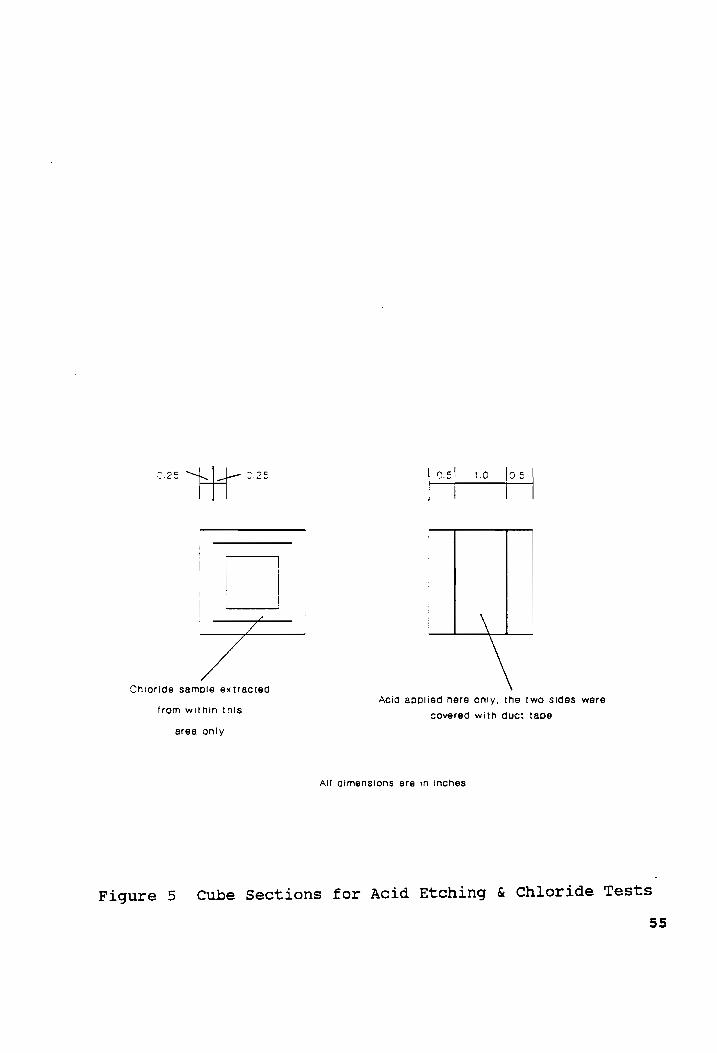
a surface dry condition. The cubes were then cut in half with

a masonry saw. From one half of each cut cube, powdered sample

was extracted with a 4%" diameter carbide drill from a square

§3

strip of width 4". The beginning edge of the strip was 4%" from

the edge of the cubes (see Figure 5). The sampling depth was

Jem,

The samples were tested for chloride content using the

specific ion probe from James Instruments, Inc as discussed in

the preceding section.

The other half of the cubes were etched with muriatic acid.

The acid was applied to a strip of width 1" in the center of

the cube section, while the rest of the surface was covered by

pieces of duct tape (see Figure 5). The acid was introduced on

the cubes with a glass dropper under the fume hood.

One cube which had not been impregnated nor subjected to salt

solution was also acid etched. The results are discussed in

Chapter 5.

54

©) NM an

O)

tf cn

oO

an

o Oo mn

Chicride sample extracted Acid aodlied here oniy, the two sides were

from within this covered with duct tape area only

All dimensions ars in inches

Figure 5 Cube Sections for Acid Etching & Chloride Tests

55

4.3.2 Effects of Drying Temperature on Corrosion Rates

From the results obtained in the section 4.3.1, it was evident

that a lower drying temperature should be sufficient for

effective polymer impregnation of concrete. This hypothesis is

discussed in detail in Chapter 5.

To validate the above statement, eight laboratory specimens of

the same dimensions and rebar configuration of the experiment

described in Section 4.2 (except for cover depths), were dried

using lower drying temperature criteria, polymer impregnated

and polymerized as before.

Four specimens had cover depth of 2" while the other four had

cover depth of %". Four specimens (two of each cover depth)

were dried to 150 °F at %" below the top rebar level while the

other four were similarly dried to a temperature of 180 °F.

Four other specimens (two of each cover depth) acted as

controls and were not impregnated.

All the steps in the polymer impregnation process were as

described in Section 4.2 except as noted below.

Grooves were not cut on the specimens. The impregnation was

accomplished from the top surface of the specimens. The time

of impregnation was estimated from the graph plotted

previously. For the specimens with 2" cover, the time was 50

hours while the corresponding time for the specimens with 4%"

cover was 17 hours.

56

In addition to recording ambient, surface and temperatures at

5" below top rebar level, temperatures at the rebar levels

were also recorded at regular intervals during the heating and

the subsequent cooling stages. The existing TC wire was

lengthened by attaching a piece of another TC wire. The wire

was insulated during the drying stage by wrapping aluminum

foil around it.

Wooden dikes were made, painted with a mixture of 90 % Epon

828 resin and 10 % of DETA (by weight) in order to make them

water tight and adhered on to the top of the specimens with

Silicon rubber. The monomer mixture was ponded on the top of

the specimens.

After polymerization, potential and 3LP (corrosion rate)

readings were taken as in the case of the first series of

specimens.

57

5.0 ANALYSIS OF RESULTS

5.1 Rigid Overlay Specimens

After a number of potential and 3LP readings were taken, it

was observed that the ambient temperature at the time of

measurement had a marked effect on the resultant readings. The

higher the temperature, the higher the 3LP reading and more

negative the potential value.

In order that all the data could be analyzed without

developing a temperature correction factor, all readings were

taken at room temperature which was 72 °F.

The potential values and the corresponding 3LP values both

before and after treatments indicated that post-treatment

potential values did not reflect very accurately the corrosion

activity in the specimens. While the I,,,, values in the

treated specimens showed very little active corrosion, the

corresponding potential values for most specimens were well

into the 90 % active corrosion region, that is more negative

than -350 mV. Therefore, it would seem that once corrosion had

been initiated and then abated by some treatment method, the

potential values were no longer reliable indicators of the

corrosion activity.

The I value being a more direct measure of corrosion rate corr

58

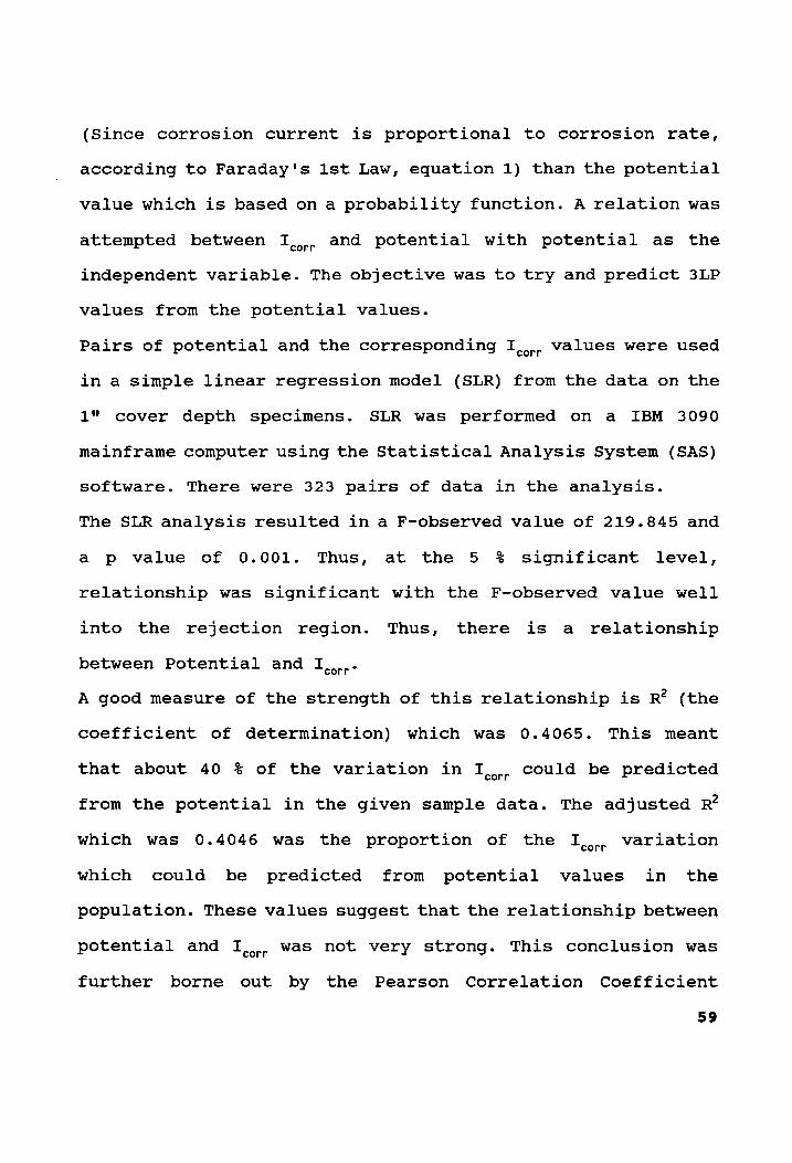
(Since corrosion current is proportional to corrosion rate,

according to Faraday's 1st Law, equation 1) than the potential

value which is based on a probability function. A relation was

attempted between I and potential with potential as the corr

independent variable. The objective was to try and predict 3LP

values from the potential values.

Pairs of potential and the corresponding I,,,. values were used

in a simple linear regression model (SLR) from the data on the

1" cover depth specimens. SLR was performed on a IBM 3090

mainframe computer using the Statistical Analysis System (SAS)

software. There were 323 pairs of data in the analysis.

The SLR analysis resulted in a F-observed value of 219.845 and

a p value of 0.001. Thus, at the 5 % significant level,

relationship was significant with the F-observed value well

into the rejection region. Thus, there is a relationship

between Potential and I,,,..

A good measure of the strength of this relationship is R* (the

coefficient of determination) which was 0.4065. This meant

that about 40 % of the variation in I,,.. could be predicted

from the potential in the given sample data. The adjusted R*

which was 0.4046 was the proportion of the I,,,. variation

which could be predicted from potential values in the

population. These values suggest that the relationship between

potential and I was not very strong. This conclusion was corr

further borne out by the Pearson Correlation Coefficient

59

between potential and I,,,. which was 0.64. The correlation

coefficient values will be between +1.0 and -1.0 with negative

value indicating negative correlation between the two factors.

The closer the positive correlation value is to +41.0, the

stronger is the relationship between the two factors.

The low values of R* and the correlation coefficient indicated

that the relationship between potential and I was not very corr

strong and it was not possible to predict I,,,, values from

potential values with a high degree of certainty.

In view of the above results, only I,,,, values were used for

comparative analyses.

For convenient display oof information, the data was

transformed into graphs and divided into three treatment

groups.

The controls (CO), LMC overlaids (LM) and LMC overlaid-

polymer-impregnated specimens (PM) were compared as_ one

treatment group. The controls, LSDC overlaids (LS) and LSDC

overlaid-polymer-impregnated specimens (PS) were compared as

the second group. Controls polymer impregnated specimens (PC)

were the third treatment group. The treated specimens in the

three groups will be referred to from now on as the latex

group, low slump group and polymer impregnated group,

respectively.

In graphs and tables, the cover depth(s) in inches and the

drying temperature(s) in °F of the specimens discussed therein

60

have been indicated in parenthesis following the caption.

The mean measurement is the average of six readings obtained

from each series of specimens, each time readings were

taken. The individual readings are presented in Appendix

Cc.

The pre-treatment potential values started with values ranging

from about -225 mV to -260 mV which is more or less in the 90

% no-corrosion region. During the course of the next fifty

days the values became less negative or the steel became more

noble with respect to corrosion activity. See Figures 6A, 6B

and 6C. This phenomenon was due to the formation of a passive

layer of gamma iron oxide around the steel which protects the

rebar from further corrosion activity.

After 50 days, the chlorides in the vicinity of the rebar

progressively destroyed the passive layer resulting in more

negative potential values. At day 214, all the specimens had

potential values more negative than -350 mv, that is in the 90

% active-corrosion region.

Chloride contents were taken on selected specimens on day 71

and again on day 190. At day 190 the chloride content at a

depth of 1 to 1%" (rebar level) for all the tested specimens

were well over the accepted threshold level for corrosion

initiation, viz. 1.2 lb/yd*. See Appendix Cc.

The third method for monitoring degree of corrosion was

the I values obtained from the 3LP device. As with the corr

61

550

500 -

450 a

400 -

E 350 ad woo Lf 250+—# Ka

150 ~ _ , , 0 50 100 150 200

Figure 6A Pre-Treatment Mean Potential (1", 230 °F)

AGE OF CONCRETE (DAYS)

—=— CO —— LM — PM

Latex Group

250

62

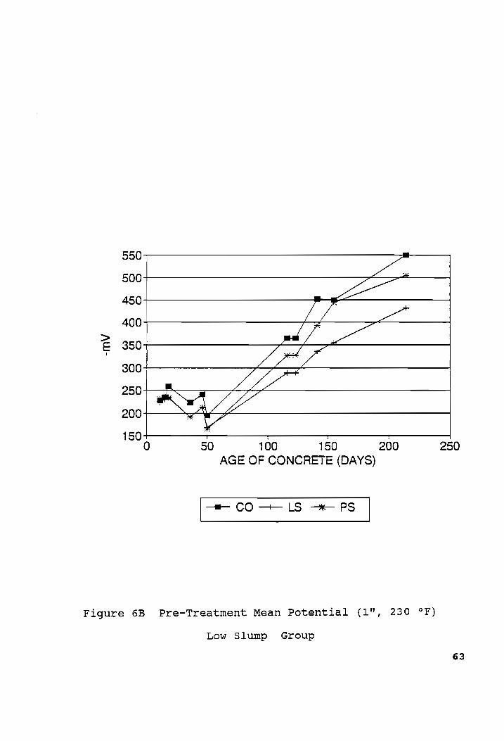
550

500

450

400

350

300

250

200

150

-mV

Figure 6B Pre-Treatment Mean Potential (1", 230 °F)

SUZ

50 100 150 AGE OF CONCRETE (DAYS)

—#t CO —— LS —«— PS

Low Slump Group

200

250

63

550

500

450

400

350

300

250

200

150

-mV

Figure 6C Pre-Treatment Mean Potential (1", 230 °F)

= mn Se q

50 100 150 AGE OF CONCRETE (DAYS)

—m CO —-— PC

Polymer Impregqnated Group

200

250

64

potential values, the mean of six readings were used for

evaluation. The individual readings are presented in Appendix

C. The mean I.,,, value at day 214 was over 2 mA/sq ft for all

the six series of specimens excepting the latex modified

concrete overlay specimens. The low value for this series was

a result of several rebars having lower than usual values at

that point in time.

The specimens were prepared for the different treatment

methods after day 214. Since it took about 33 days for the

entire process of treatments to be completed, it can be safely

assumed that at the actual time of treatments the corrosion

levels were higher than what was indicated at day 214.

For reasons cited, the post-treatment potentials were not used

for evaluation. The mean post-treatment potential values are

presented in Figures 7A, 7B and 7C.

The mean values of the corrosion current (see Figures 8A, 8B

and 8C) indicated that the control specimens progressively

corroded to extremely high levels with the passage of time,

while in all the treated specimens the corrosion levels

dropped and then did not show appreciable fluctuation over

time.

Since the last pre-treatment values had a significant range

for the different series of specimens, the absolute mean post-

treatment values is not a good measure for comparing the

effectiveness of the five treatment methods with each other

65

0 i l |

0 50 100 150 200 DAYS AFTER OVERLAYS (Days)

——-coO j—>-LM —<—PM

Figure 7A Post-Treatment Mean Potential (1", 230 oF)

Latex Group

66

300 Ne

NN 200

100 0 el !

0 50 100 150 200 DAYS AFTER OVERLAYS (Days)

co ~LS —-*<PS

Figure 7B Post-Treatment Mean Potential (1", 230 °F)

Low Slump Group

200 Say

100

0 ! ! l

0 50 100 150 200 DAYS AFTER OVERLAYS (Days)

—=- CO —> PC

Figure 7C Post-Treatment Mean Potential (1", 230 °F)

Polymer Impregnated Group

68

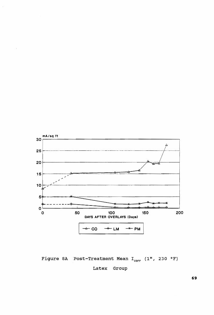
mA/sq ft

25 - oe é

~ an 15 oe = =

10 = a”

5 wake

fo ee 0 —— : |

0 50 100 150 200 DAYS AFTER OVERLAYS (Days)

—~—- CO ——— LM —— PM

Figure 8A Post-Treatment Mean I,,,. (1", 230 °F)

Latex Group

69

mA/sq ft

30

20}-- poms f

77 15 fe = =

10--<- ae

- 3 0 | al : l

0 50 100 150 DAYS AFTER OVERLAYS (Days)

-4—- CO —LS —— PS

Figure 8B Post-Treatment Mean I,,,, (1", 230 °F)

Low Slump Group

200

70

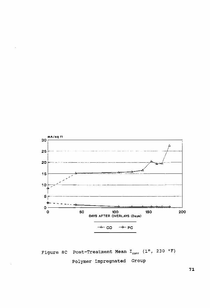
mA/sq ft

30:

20 lan /

15 a =

10 -->— &

5

a

0 — de ee eee

O 50 100 150 200 DAYS AFTER OVERLAYS (Days)

co PC

Figure 8C Post-Treatment Mean Liorr (1%, 230 °F)

Polymer Impregnated Group

721

and with the control specimens. Therefore the % change in each

post-treatment value was computed on the basis of the last

pre-treatment value as follows:

% change = {(B - P)/B} x 100 (3)

where,

B = last pre-treatment I in mA/sq ft, and corr

P present I in mA/sq ft. corr

Therefore, a positive value of "% change" indicates that

corrosion rate has decreased from its pre-treatment level,

while a negative value of "% change" signifies a higher

corrosion level compared to its pre-treatment value.

At day 181 after the application of the overlays, the control

specimens had % change as -223.4 demonstrating the extreme

deteriorated condition of the untreated specimens. See Figure

9A, 9B and 9C. The latex group and polymer impregnated groups

demonstrated values of over +50 % at day 181. The

corresponding figures for the low slump group were well below

+50 % improvement level. However, they remained in the

positive range indicating that the treatments did have the

desired effect of reducing corrosion levels. The low slump

overlay specimens had a value of +22.7 % while the low slump

overlay with polymer impregnation had a slightly higher value

of +36.2 4%.

72

100

% CHANGE

Figure 9A Percent Change in Mean I

\

‘

60

80 100 120 140 160 180 200 DAYS AFTER OVERLAYS (DAYS)

—=m CO —— LM — PM

(1", 230 °F) corr

Latex Group

% CHANGE

100

\

‘ 4

40 60 80 100 120 140 160 180 200 DAYS AFTER OVERLAYS (DAYS)

—= CO-—- LS —*- PS

Figure 9B Percent Change in Mean I,,,, (1", 230 oF)

Low Slump Group

100 7 —

% CHANGE

3 Oo

0 60 80 100 120 140 160 180 200

DAYS AFTER OVERLAYS (DAYS)

—m CO —— PC

Figure 9C Percent Change in Mean I (1", 230 °F) corr

Polymer Impregnated Group

75

At 41 days after overlays, all series of treated specimens,

except for the polymer impregnated specimens had negative

values of "% change". A possible explanation is that there is

a time lag before the overlays cause a decrease in the

corrosion rates.

The absolute difference in the "% change" between the last and

first values may be a useful measure of the effectiveness of

each treatment procedure. See Table 1.

The maximum value of this measure was 91.03 %* for the LSDC

specimens and the minimum value was 42.30 % for the polymer

impregnated specimens. There seemed to be no well defined

trend between the three groups. This indicated that there was

no appreciable difference in the effectiveness of any

treatment method. The specimens with only = overlays

demonstrated higher values than their counterparts which were

polymer impregnated in addition to the overlays. This would

seem to indicate that impregnation had decreased the

effectiveness of the overlays in abating corrosion.

However, both the series with overlays and polymer

impregnation, the PM series (LMC overlay-polymer-impregnation)

and the PS series (LSDC overlay-polymer-impregnation) had the

highest pre-treatment corrosion rates of 4.99 mA/sq ft and

4.92 mA/sq ft, respectively. It is conceivable that these

higher corrosion rates had an effect on the "absolute

difference in % change" values. It is reasonable to expect

76

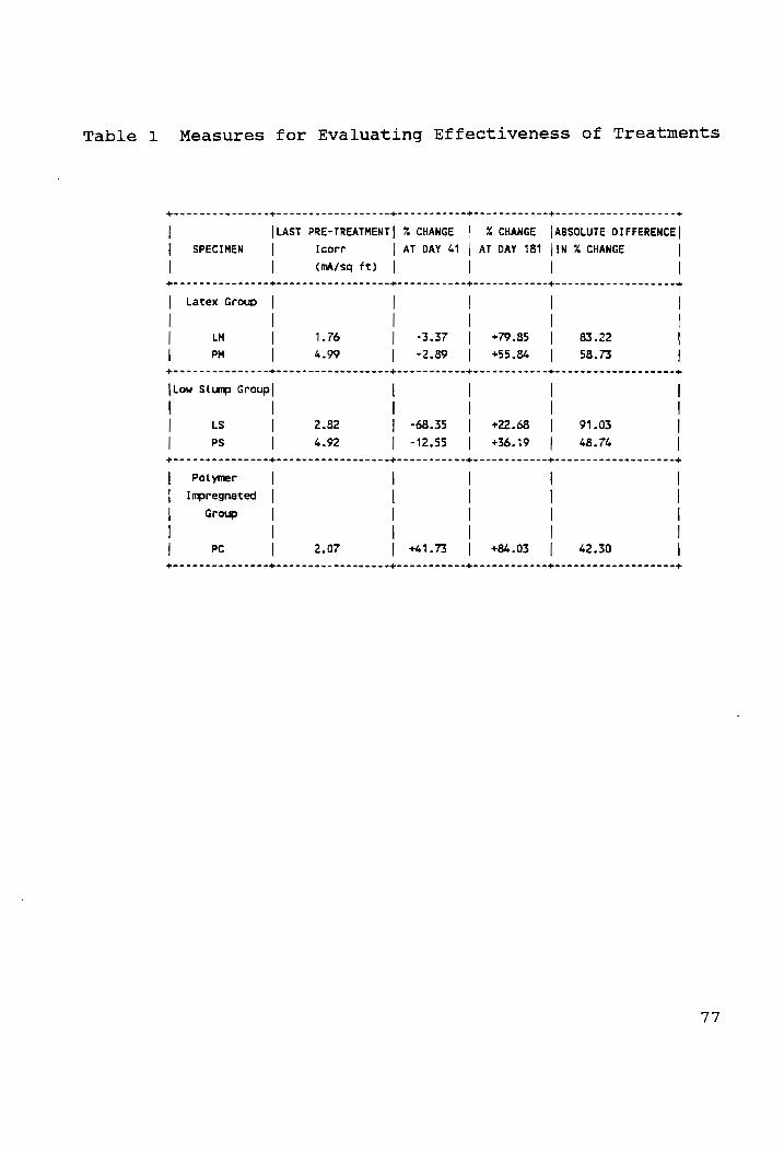
Table 1 Measures for Evaluating Effectiveness of Treatments

Pewee weeewsenccven Pecceeesenecrewrncce Pecan acnetaecen

|LAST PRE-TREATMENT | % CHANGE | | | SPECIMEN

| Peewee sewweesocce

| Latex Group

| | LM

| PM peweceeccecawswe=

| Ls | PS

Polymer

Impregnated

| | | Group

| |

Icorr

(mA/sq ft)

eaeanan en nanos easeee

AT DAY 41

$e

g¢ — — — —

g¢ — —

—

gt

% CHANGE

AT DAY 181

+ ‘ ’ ‘ ‘ ‘ ‘ a ‘ ‘ ‘ ‘ ‘ ‘ ‘ ‘ t ‘ ‘ ’ +

{ABSOLUTE DIFFERENCE |

|1N % CHANGE |

| | Peewee were er ececaue +

| | | | | 83.22 |

| 58.73 | bocce wee eter ese ewene +

| | | | | 91.03 |

| 48.74 | eee ween ee wceecnneoe +

| | |

| | | | | 42.30 |

eee ccen wn nccccevcee +

77

that any treatment method would be more effective if the

initial corrosion rate was low than the case where the initial

corrosion rate was relatively higher. For a better analysis of

the situation, the post-treatment corrosion rates should be

monitored for a longer period of time than could be

accommodated in the scope of this study.

From a comparison of the actual values of "% change", the low

slump group appeared to have lower effectiveness as compared

to the other two groups. As have been mentioned before, this

measure might not be a very accurate representation of the

situation, since it does not indicate the 'degree' of the "%

change".

The values of the "% change" at day 41 (see Table 1) indicated

that the low slump group also had been least effective in

abating corrosion at this age. However, specimens which had

been overlaid with LSDC (LS) had an unusually high negative

value of "% change", viz. -68.35 % which was comparable to the

"3 change" of the control specimens at the same point in time,

-79.47 %. The much lower negative value of "% change" (-12.55

%) in the specimens with LSDC overlay-polymer-impregnation

(PS) could probably be attributed to the polymer impregnation.

However, this value for the PS series was more negative than

the other groups. The higher pre-treatment corrosion rates

could not be forwarded as a possible cause, since the

specimens with LMC overlay-polymer-impregnation (PM) also had

78

similar high pre-treatment corrosion rates. In the case of the

PM series, the "% change" at day 41 was -2.89 % which was

comparable to the -3.37 % value for the LMC overlay (LM)

specimens.

A possible explanation for the apparently lower effectiveness

of the low slump group is that the low design slump of LSDC

overlay resulted in imperfect compaction after the overlay was

placed. The LSDC overlay had a rough surface which suggests

the presence of more void spaces resulting in increased

permeability for more rapid ingress of chloride ions after

treatment.

79

5.2 Influence of Cathode to Anode Area on Corrosion Rates

The standard electrical connections had a cathode to anode

surface area (C/A) of 2. In order to study the influence of

the C/A on corrosion rates, corrosion current readings were

taken with different electrical connections such that the C/A

were 1, 2, 3 and 4 as shown in Figures 10A and 10B. In each

case, the anode involved was the right anode of each specimen.

The left anode was kept isolated in order to obtain the micro-

cell corrosion values. After each C/A connection type was

completed, the specimen-system was allowed to stabilize for at

least one day before readings were taken.

When I.,.. readings were taken with the cathode and anode being

separated by a distance, the obtained values were a mixture of

micro-cell and macro-cell corrosion current, or mixed-cell

corrosion current.

Effect of C/A on Mixed I,,,,

Change in C/A did not have appreciable effect on the corrosion

current for the five treatment methods. See Figures 11A, 11B

and 11C. The corrosion abatement techniques had substantially

decreased the corrosion rates, and increased cathode area had

little influence in changing the corrosion rate. Thus, some

80

O O \ \ C/A = 2

Figure 10A Different Electrical Connections Used

C/A = 1, 2

81

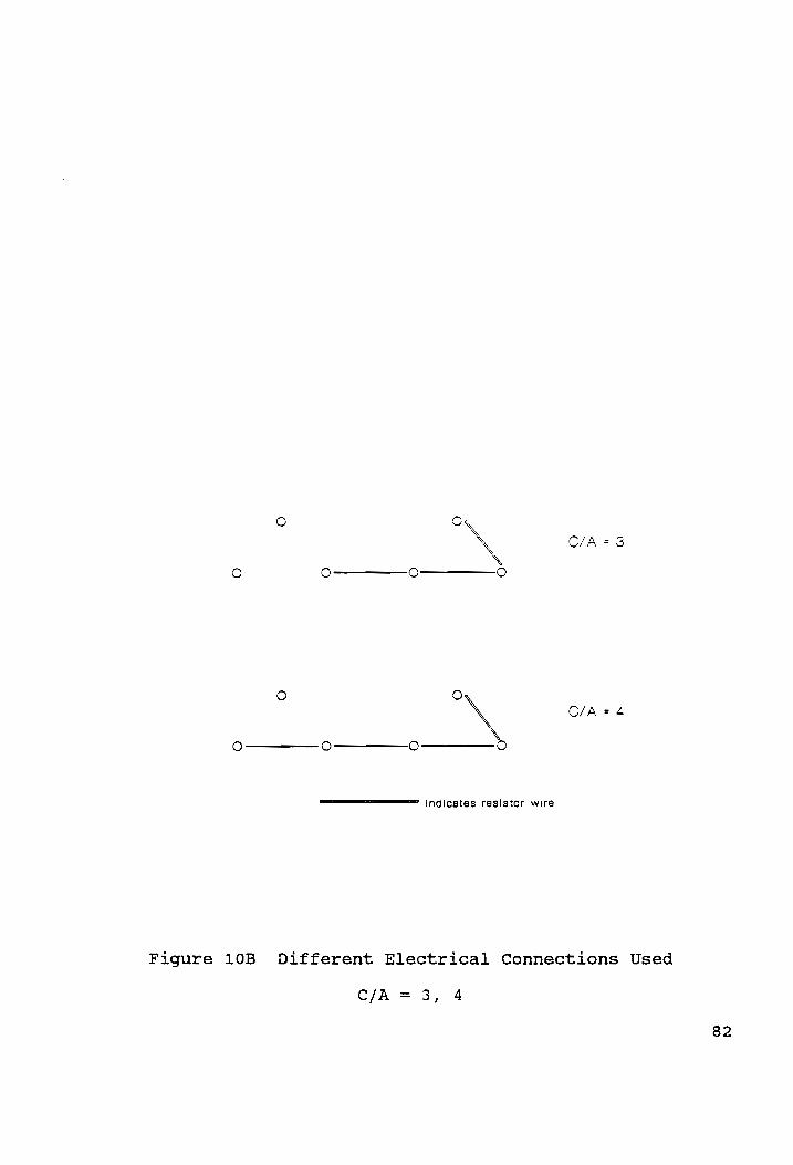
O oO \ C/A = 4

indicates resistor wire

Figure 10B Different Electrical Connections Used

C/A = 3, 4

82

=

mA/sq

20 18

12

10

ON fF

OD

|

C/A

—a— CO —— LM —* PM

Figure 11A Mixed I vs C/A (1", corr

Latex Group

230 °F)

83

mA/s

q ft

20

18

16

14

12

10

oO NM

fF

OD @W

Figure 11B Mixed I

C/A

— CO —— LS —*- PS

vs C/A (1", 230 °F) corr

Low Slump Group

84

Figure 11C Mixed I vs C/A (1", corr

Polymer Impregnated Group

230 °F)

85

other factor is controlling the corrosion rate of the treated

specimens. Possible factors are chloride content, temperature,

moisture content, available oxygen and resistance between the

cathode and anode. Of these factors, the temperature, moisture

content and available oxygen were more or less constant for

the different C/A ratios. The chloride content could not have

changed much, as all the readings with different C/A ratio

were taken in a time span of nine days. However, resistance

increases with increasing C/A ratio. Therefore, the inherent

increment in I,,,. with increase of C/A ratio was neutralized

by the corresponding increase in resistance. Consequently,

there was insignificant net change in the corrosion current.

For the case of the control specimens, the corrosion rate

(I was much higher and thus it was more sensitive to corr)

changes in C/A ratios. For C/A ratio between 1 and 2 and

between 2 and 3, the I... showed decrements; a sharp drop

followed by a more gradual decrease. In this region of the

graph, the higher resistance not only negated the effect of

the increase in C/A ratio but actually caused the I,,,. to

decrease. However between C/A ratio 3 to 4, the larger cathode

area appears to have had an influence resulting in an increase

in the corrosion current which returned to approximately the

same rate as the C/A ratio of 1.

86

Effect of C/A on Macro-cell Corrosion

The macro-cell corrosion current were measured in mA for the

corroding system. Individual readings are presented in

Appendix C. For comparison purposes with the micro-cell and

mixed-cell corrosion rates, the macro-cell current was

converted to mA/sq ft for the corroding systems.

The corroding surface area was the uncovered portion of the

anode which was 6.5" long. Therefore, the requisite surface

area is given by: {m(d/2)* x 6.5} square inches; where, d =

diameter of rebar in inch. Substituting 5" for 'd', the area

is 10.21 sq.in. or 0.0709 sq.ft. Hence, to convert values from

mA to mA/sq ft, the multiplicative factor is 1/0.0709 =

14.10382 was used.

As shown in Figures 12A, 12B and 12C, the changes in macro-

cell corrosion current with increasing C/A ratio were similar

to that of the trends observed in mixed-cell corrosion. For

the specimens which underwent the five treatment methods,

there were no significant difference in the macro-cell current

with changing C/A ratio. However, for the control specimens

the macro-cell current increased significantly with increase

in C/A ratio.

87

mA/s

q ft

1.2

ss Z 0.6 WA

0.4

0.2 a

f.

-H+

1 2 3 C/A

—#— CO —— LM —* PM

Figure 12A Macro I vs C/A (1", 230 °F) corr

Latex Group

88

1.2 oo

Z

0.8

0.6 Lf

0.2 Zo —_—_——_————

<_

0 . | — | 1 2 3 4

C/A

—=s CO-+—-LS -*- PS

Figure 12B Macro I,,,, vs C/A (1", 230 °F)

Low Slump Group

89

mA/s

q ft

1.2

0.8

0.6

0.4

0.2

Figure 12C Macro I

vs C/A (1", 230 °F) corr

Polymer Impregnated Group

90

Change of Micro-cell I,,.. over time

The treated specimens showed little change in the micro-cell

current over a period of six days. See Figures 13A, 13B and

13C. As the corrosion level had been reduced, there were very

little corrosion activity to reflect any change in their

values over time.

In the control specimen, on the other hand, the micro-cell

I increased with time as expected, since the active corr

corrosion of these specimens increased with time.

Comparison Between Micro-cell and Mixed-cell Corrosion

There was little difference between the micro-cell and mixed-

cell corrosion for the treated specimens for the same reasons

stated previously. For the control specimens, which were

actively corroding the difference was apparent. See Figures

14A, 14B and 14C.

91

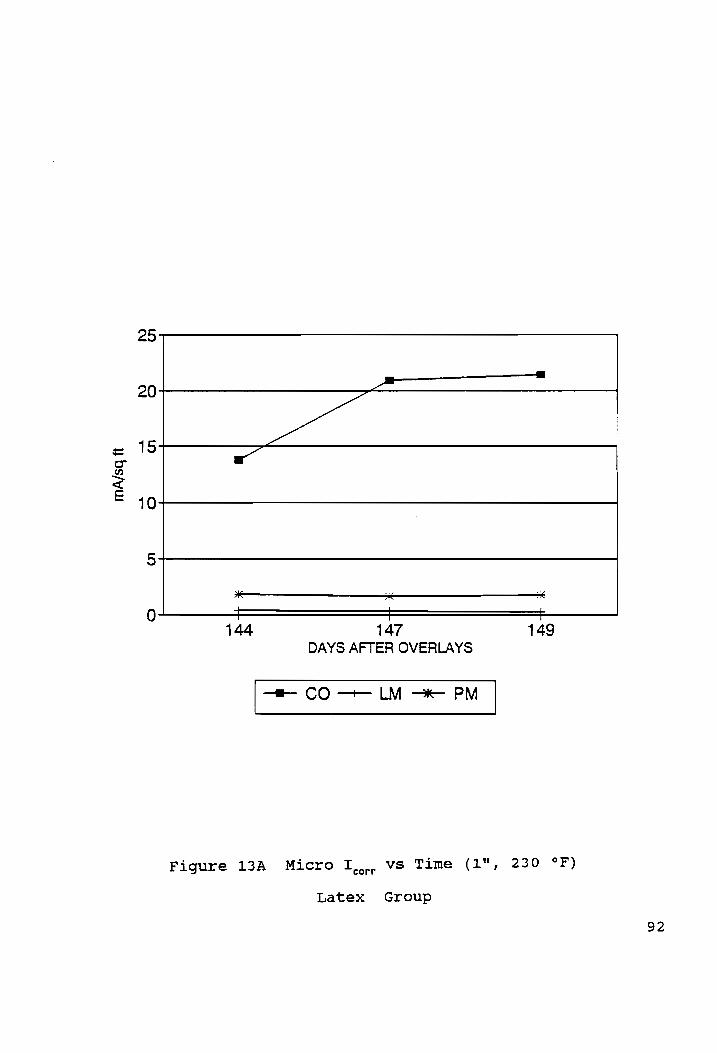
25

a

mA/s

q ft

wes —~ +

144 147 149 DAYS AFTER OVERLAYS

—™m CO —~- LM —- PM

Figure 13A Micro I vs Time (1", 230 °F) corr

Latex Group

92

25

— ij

15 c — uf

< E 40

5 x x

0 - 144 147 149

DAYS AFTER OVERLAYS

—= CO—-—-LS —-* PS

Figure 13B Micro I vs Time (1", 230 °F) corr

Low Slump Group

93

mA/sq

ft

25

= —ai

: ea

15 —

10

5

0 “ _

144 147 149 DAYS AFTER OVERLAYS

—= CO —— PC

Figure 13C Micro I vs Time (1", 230 °F) corr

Polymer Impregnated Group

94

mA/s

q ft

20

18

16

14

Oo

N

Ff

OD WD

OO

_— Pee

——~

MIXED MICRO lcorr TYPE

—=— CO —— LM —* PM

Figure 14A Mixed and Micro I,,,, (1", 230 °F)

Latex Group

95

mA/sq

ft

18 —

16 ~~.

14 —~_

12

10

8

6

4 wag

2 —— -

° MIXED MICRO Icorr TYPE

—m— CO—-—- LS —* PS

Figure 14B Mixed and Micro I,,,, (1", 230 °F)

Low Slump Group

96

mA/sq

ft

oO

N

Ff DO

BD

OD

20

18

16

12

Figure 14C Mixed and Micro I

a

MIXED lcorr TYPE

~ MICRO

—™ CO —-— PC

corr (1", 230 °F)

Polymer Impregnated Group

97

Comparison Between Micro-cell and Macro-cell Corrosion

As shown in figures 15A, 15B and 15C, the differences between

the micro-cell corrosion and macro-cell corrosion were more

pronounced for all the specimens than their corresponding

differences between micro-cell and mixed-cell corrosion. This

was expected since a major portion of corrosion current is due

to the micro-cell.

98

mA/s

q ft

14 YO

12

; \

AL __--—_

MICRO MACRO lcorr TYPE

—= CO —— LM —* PM

Figure 15A Micro and Macro I (1", 230 °F) corr

Latex Group

99

mA/s

q ft

14 \

12 \

10

\

| oN —$__

MICRO MACRO lcorr TYPE

—= CO—-— LS —* PS

Figure 15B Micro and Macro I,,,, (1", 230 °F)

Low Slump Group

100

mA/s

q ft

14 \

12

A \

MICRO MACRO {corr TYPE

—s— CO — PC

Figure 15C Micro and Macro I (1", 230 °F) corr

Polymer Impregnated Group

101

5.3 Pre-impreqnation Drying of Specimens

Three drying temperatures were used in this study: 150 °F, 180

°F and 230 °F. The drying temperatures refer to the

temperature at 4%" below the top rebar level at the time the

heaters were turned off.

Drying Temperature 230 °F : Cover Depth 3" (2" overlay plus 1"

cast)

Of the nine specimens that were dried to this temperature, the

polymer impregnated (PC) series without an overlay and thus

with a cover depth of only 1" attained the requisite

temperature before the other specimens (see Figure 16). To

minimize further increase in temperature while the other

specimens were being dried to the requisite temperature, the

PC specimens were covered with metal sheet. In spite of this,

the temperature of the PC series continued to increase

The mean temperature of the LSDC overlay-polymer-impregnation

(PS) series five minutes before heaters were shut off was less

than 230 °F due to the fact that one of the three PS

specimens had an unusually low temperature. It can be safely

assumed that at the time the three heaters were shut off,

eight of the nine specimens had temperatures close to 230 °F

102

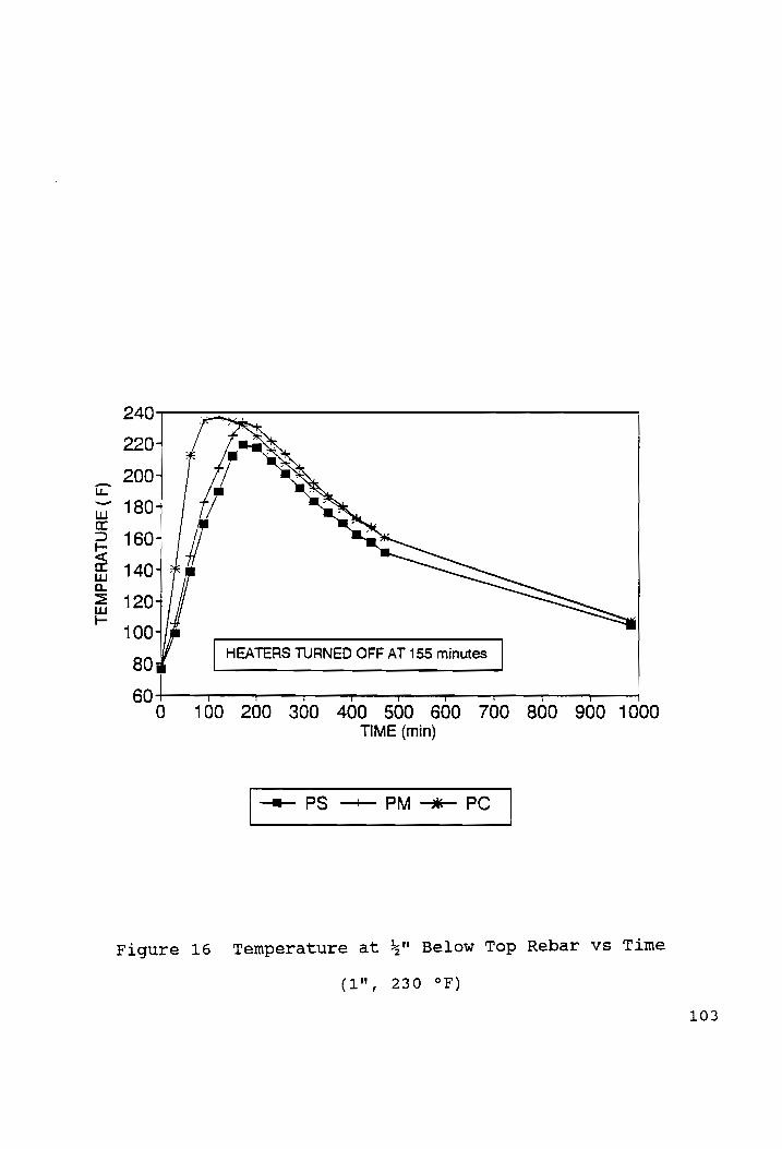
TEMP

ERAT

URE

( F)

240

220-

2007

1807

1607

1407 >

120-

100-/" 80 HEATERS TURNED OFF AT 155 minutes

60 r —— - — QO 100 200 300 400 500 600 700 800 900 1000

TIME (min)

—m—- PS —— PM —-* PC

Figure 16 Temperature at 4%" Below Top Rebar vs Time

(1", 230 °F)

103

or above at 4" below the top rebar level. The only specimen

(PS2) which may have had a lower temperature could have had a

faulty TC or connection which would cause a discrepancy in the

temperature readings.

After the heaters were turned off, the internal temperature of

most of the overlaid specimens continued to rise. This was not

the case for the PC series which did not have an overlay.

Concrete being a heat sink, the heat energy from the surface

continued to be absorbed by the concrete below thereby

increasing the internal temperature for a period of time after

the heaters were turned off. Predictably, this phenomenon

would be more pronounced with increased concrete depth as

shown in Figure 16. After the heaters were turned off, the

internal temperatures of the overlaid specimens increased

between about 5 °F to 10 °F. The drying time was about 2%

hours.

During the cooling period, the surface and internal

temperature approached each other and at about 1000 minutes

(from the beginning) the surface and internal temperatures

were nearly equal. Concrete retains heat for a long period of

time and this was evident from the fact that even after 850

minutes from the time the heaters were turned off (1000

minutes from the beginning) the internal temperature was over

100 °F with an ambient temperature of about 50 °F (see Figure

17).

104

600

500-

400-

300- HEATERS TURNED OFF AT 155 minutes

200-

TEMP

ERAT

URE

(F)

—_

© © 1 | —ai

0 T r , ~E T 1 T T ,

O 100 200 300 400 500 600 700 800 300 1000 TIME (min)

—=@- AMBIENT —+— SURFACE

Figure 17 Surface and Ambient Temperature vs Time

(1", 230 °F)

105

During the heating, the surface temperature reached a maximum

of 529 °F (see Figure 17) and then decreased sharply after the

heaters were turned off. After which, for a period of about

two hours, the rate of cooling was more gradual.

3 Drying Temperature 150 °F and 180 °F (Cover Depths: 4%" and 2")

Cover depth: 2"

After the heaters were turned off, the temperature increase at

5" below top rebar for the four specimens were between 8 °F

and 18 °F (see Figures 18A and 18B). Two of these specimens

(PM2 & PC3) were covered with sheet metal before the heaters

were turned off. As a result, the temperature rise may have

been somewhat less than what would have normally occurred if

they were covered with insulation immediately after the

heaters were turned off.

The drying time was approximately one hour.

Cover depth: 3%"

Increases in temperature after the heaters were turned off

were between 20 °F and 24 °F (see Figures 18C and 18D).

The drying time was about 4 hour.

106

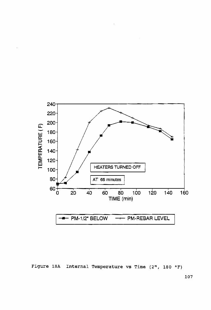
240

2207

2007

180-

160-

140-

1207

100°

TEMPERATURE

( F)

HEATERS TURNED OFF

AT 65 minutes

60-+ = 7 T T T —T y

0 20 40 60 80 100 120 140 £2160 TIME (min)

—@— PM-1/2" BELOW -—+— PM-REBAR LEVEL

Figure 18A Internal Temperature vs Time (2", 180 °F)

107

200

180- JON

a 160 - LL

5 _

= HEATERS TURNED OFF AT LL QO.

.

= 64 minutes LL -~

60-7 q T T T T

Q 20 40 60 80 100 120 140 #4160 TIME (min)

t C

Figure 18B Temperature at &" Below Top Rebar vs Time

(2", 150 °F)

108

260 240- 2207 200 180- 160- 140- 120- 100- 80

TEMPERATURE

( F)

HEATERS TURNED OFF

AT 30 minutes

60 qT = ”

20 40 60 80 100 120 140 TIME (min)

—™— PM-1/2" BELOW -—— PM-REBAR LEVEL

Figure 18C Internal Temperature vs Time (%", 180 °F)

109

240

220+

_ 2007 i ~ 180;

cc 160; —

Ee 140- i 420- HEATERS TURNED OFF ou. = 4 iL 100 AT 25 minutes

804

60

40 q ot v + y

0 20 40 60 80 100 120

TIME (min)

—m— PC-1/2" BELOW -—— PC-REBAR LEVEL

Figure 18D Internal Temperature vs Time (%", 150 °F)

110

5.4 Optimization of Drying Temperature

The following analysis is with reference to Table 2.

With the increase in drying temperature, %* volume of water

lost increased, as more water was driven out of the cubes.

At 75 °F, % volume monomer gained was 20 % and the value at

100 °F was 10.5 %. At 125 °F, % volume monomer gained was 8.8

oe

At higher drying temperatures, %* volume monomer gained

increased with increasing drying temperatures up to 400 °F and

remained constant afterwards at 10.3 % (see Figure 19). The

cubes at 75 °F were visibly cracked after the impregnation

stage and the high monomer content was probably due to direct

physical entry of some monomer into the cracked cubes rather

than entry only by diffusion. Although the cubes at 100 °F

were not visibly cracked the anomaly in the monomer content

might be due to direct entry of monomer via micro-cracks

invisible to the unaided eye.

The difference in volume between water lost and monomer gained

-increased with drying temperature. Thus, at higher drying

temperatures, water accessible voids were not being refilled

with monomer. A possible explanation is that, monomer

molecules being large organic molecules, were filling voids to

a certain limiting size. Voids smaller than this limit could

not be filled with the large monomer molecules.

The moisture content values following vacuum saturation of the

111

Table 2 Results from Impregnated Cubes

VOLUME OF VOLUME OF MOISTURE CONTENT

ORYING WATER LOST POLYMER AFTER VACUUM

TEMP DURING DRYING GAINED OL FFERENCE SATURATION

€ FY (4) (%) (4) (%)

73 - 20.0* - -

100 13.2 10.5** 2.7 0.75

125 14.0 8.8 5.2 0.70

150 15.5 9.3 6.2 0.85

175 15.3 9.7 5.6 0.70

200 16.0 9.7 6.3 0.37

225 16.5 9.5 7.0 0.58

250 16.6 9.0 7.6 0.52

300 17.1 10.0 7.1 0.44

400 18.3 10.3 8.0 0.59

500 19.2 10.3 8.9 0.68

600 20.2 10.3 9.9 0.92

CONTROL - - - 2.67

* CUBES FRACTURED DURING IMPREGNATION

** POSSIBLE MICRO CRACKS DURING [MPREGNATION INVISIBLE

TO THE UNAIDED EYE

112

Table 2 Results from Impregnated Cubes (Contd.)

RESISTIVITY RESISTIVITY

DRYING BEFORE SALT AFTER SALT DIFFERENCE IN CHLORIDE

TEMP APPLICATION APPLICATION RESISTIVITY CONTENT

( F) ¢€1000 ohm-cm) (1000 ohm-cm) (1000 ohm-cm) (lb/cu yd)

75 - - - -

100 406 13.2 392.8 0.61

125 401 12.5 388.5 0.66

150 350 13.2 336.8 0.65

175 654 20.7 633.3 0.65

200 793+ 20.5 772.5 0.61

225 490 26.0 464.0 0.62

250 313 16.8 496.2 0.60

300 849 34.3 814.7 0.60

400 487 57.8 429.2 0.55

500 267 35.5 231.5 0.57

600 200 27.3 172.7 0.54

CONTROL 4.8 2.8 2.0 14.38

b+ MEAN FROM TWO CUBES; THIRD CUBE HAD VERY HIGH VALUES

113

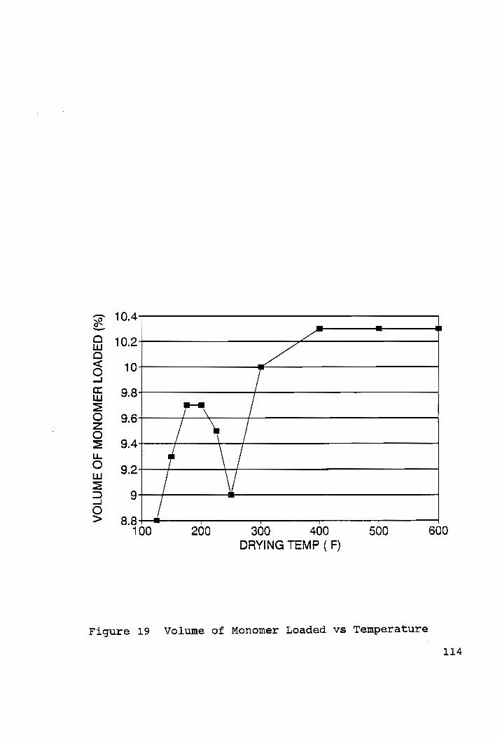
10.4 ‘ 7

10.2 Za

—

©

9.8 96 pr /

aw

VOLUME

OF MONOMER LOADED

(%)

22 : LT

8.8- T T T T

100 200 300 400 500 600

DRYING TEMP ( F)

Figure 19 Volume of Monomer Loaded vs Temperature

114

cubes are presented in Figure 20. The lowest value of moisture

content was at 200 °F. After this, the moisture content

increased with increasing temperatures. At temperatures below

the boiling point of water, the higher moisture contents are

the result of water remaining after drying. At higher

temperatures, more water could fill the smaller voids which

the monomer could not fill. At 200 °F, most of the available

void spaces had been filled by the monomer molecules,

resulting in the low moisture content. The moisture content of

the control cubes (unimpregnated) was much higher (2.67 $%)

than any of the impregnated cubes. Thus, even at low drying

temperatures, some degree of monomer impregnation is possible.

With reference to Figure 21, the resistivity values before

salt application showed peak values at 200 °F and 300 °F and

then decreased at higher temperatures. The lowest resistivity

value was 200,000 N-cm. Previous studies [23, 24, 25, 26]

suggested different resistivity values above which corrosion

will not occur. The smallest value is 12,000 Q-cm [23, 24]

while the highest is 60,000 N-cm [25]. Thus, even if the most

conservative value was to be adopted, it would result in the

lowest obtained resistivity value being in the no-corrosion

region.

The resistivity values followed a trend which supported the

corresponding values of moisture content. Around 200 °F, the

moisture content was the lowest and the resistivity was near

115

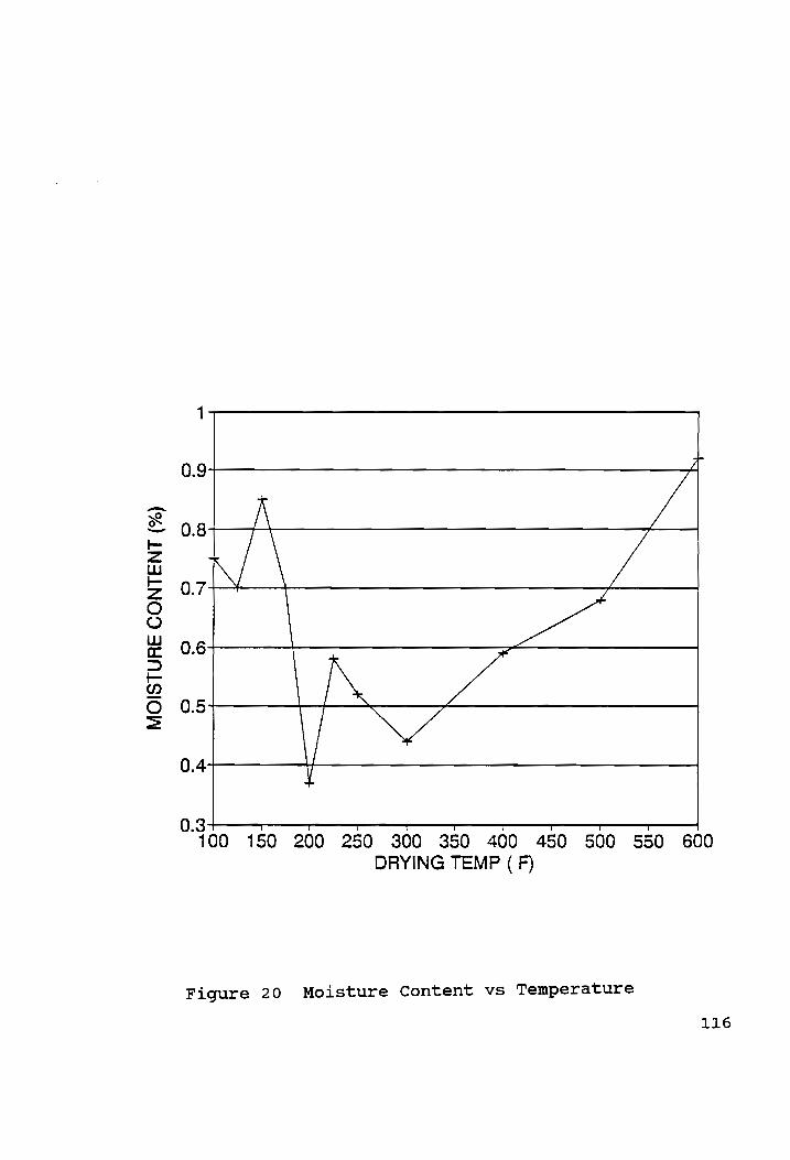
MOISTURE CONTENT

(%)

T 7

eva Z

a _ ea

oN ie 4 0.4 V 0.3 oF { i q q 1 t q q

100 7150 200 250 300 350 400 450 500 550 600

DRYING TEMP ( F)

Figure 20 Moisture Content vs Temperature

116

RESI

STIV

ITY

(1000

ohm-cm)

PRE-SALT: PRIMARY Y-AXIS POST-SALT: SECONDARY Y-AXIS

ns h_A * wo LL AZ \ wo fi} A \ te so f = —

oye Ns

DRYING TEMP (F)

—™@— PRE-SALT —+— POST-SALT

200 T T T T T T T “T" T 10

100 150 200 250 300 350 400 450 500 550 600

Figure 21 Resistivity vs Temperature

RESI

STIV

ITY

(100

0 oh

m-cm

)

117

its peak. Since, the ionic pore solution is the conducting

agent, the resistivity of concrete increases with decreasing

moisture content. Predictably, at 600 °F when the moisture

content was high, the resistivity was low.

The resistivity values after salt application were much lower

than their pre-salt application values (see Figure 21). The

trend of the post-salt application resistivity values was

similar to that of the pre-salt application ones, with respect

to drying temperatures. Apart from the large shift downwards,

there was apparently a slight shift to the right.

The values of the post-salt application resistivity were low

due to the Cl ions being present in the mortar pore water.

The value corresponding to 200 °F was 20,500 N=-cm which is

greater than the lowest suggested no-corrosion value of 12,000

N-cm, but less than the highest suggested value of 60,000 n-

cm. However, the possibility remained that the cubes were not

fully surface dry when the post-salt application resistivity

values were taken, which could have resulted in lower values

than actual.

118

Acid Etching and Chloride Content of the Cubes

Application of the acid had no discernible effect on the

impregnated cubes, as the polymer molecules prevented the

dissolving of cementitious particles. However, in the non-

impregnated cubes the cement portion was attacked by the acid.

For a more visual demonstration of this phenomenon, both

impregnated and unimpregnated cubes were colored with a

permanent marker and then etched with the acid. In the

impregnated cubes, almost all the color remained while for the

non-impregnated cubes the color started to fade after repeated

applications of the acid.

The relationship between chloride content and drying

temperature (see Figure 22) indicated that with higher drying

temperatures there was a lowering of the chloride content as

higher volume of the polymer resisted the Cl” ingress into the

cubes. The maximum value at a drying temperature of 125 °F was

0.66 lb/yd>.

For the control cubes, the chloride content was much higher

(14.38 lb/yd*) than in the impregnated cubes. With the absence

of polymer molecules, the chloride ions readily diffused into

the mortar cubes.

119

CHLO

RIDE

CO

NTEN

T (lb/cu y

d)

0.66 im

0.64

i

0.6 mt

0.58 \

0.56 wo

0.54 T T T T T 7 = = r -

100 150 200 250 300 350 400 450 500 550 600 DRYING TEMP ( F)

Figure 22 Chloride Content vs Temperature

120

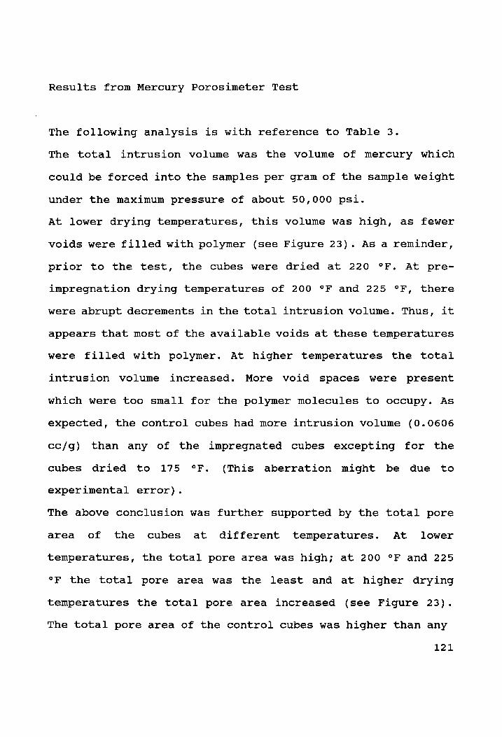
Results from Mercury Porosimeter Test

The following analysis is with reference to Table 3.

The total intrusion volume was the volume of mercury which

could be forced into the samples per gram of the sample weight

under the maximum pressure of about 50,000 psi.

At lower drying temperatures, this volume was high, as fewer

voids were filled with polymer (see Figure 23). As a reminder,

prior to the test, the cubes were dried at 220 °F. At pre-

impregnation drying temperatures of 200 °F and 225 °F, there

were abrupt decrements in the total intrusion volume. Thus, it

appears that most of the available voids at these temperatures

were filled with polymer. At higher temperatures the total

intrusion volume increased. More void spaces were present

which were too small for the polymer molecules to occupy. As

expected, the control cubes had more intrusion volume (0.0606

cc/g) than any of the impregnated cubes excepting for the

cubes dried to 175 °F. (This aberration might be due to

experimental error).

The above conclusion was further supported by the total pore

area of the cubes at different temperatures. At lower

temperatures, the total pore area was high; at 200 °F and 225

°F the total pore area was the least and at higher drying

temperatures the total pore area increased (see Figure 23).

The total pore area of the control cubes was higher than any

121

Table 3 Data from Porosimeter Test

DRYING TL INTRUSION TOTAL PORE AVERAGE 4

TEMP VOLUME AREA PORE DIA CAPILLARY

( F) (cc/g) (sq m/g) (micrometers)

100 0.0518 5.2038 0.0398 7.5823

125 0.0435 5.7887 0.0300 7.0170

150 0.0520 6.0464 0.0344 7.7263

175 0.0693 7.1469 0.0388 9.2071

200 0.0080 1.0022 0.0319 0.9541

225 0.0042 0.2114 0.0795 0.9501

250 0.0185 1.0314 0.0716 2.9150

300 0.0544 5.8839 0.0370 6.7780

400 0.0426 5.7121 0.0298 6.4912

500 0.0419 6.1251 0.0273 7.0573

600 0.0367 5.3034 0.0277 5.1400

CONTROL 0.0606 7.9242 0.0306 7.0250

122

0.07 8

Sool A & 0.06 7s

a & = 0.057 A Po ——_ rE oS

3 w/ SL

O | -5 =< > 0.04 << #

3 | / M3 Q 0.03 aa

z | 8 E 0.02 lo

2 |_/) : <= 0.01 4 O WY

0 T T T T 0

100 200 300 400 500 600

DRYING TEMP ( F)

—a— TLINTRU VOL —— TL PORE AREA

Figure 23 Intrusion Volume & Pore Area vs Temperature

123

of the impregnated cubes (see Table 3).

The average pore diameter showed a decrease at temperatures

over 250 °F. This indicated that in spite of larger total pore

area at higher temperatures, the average pore diameter of

accessible pores is smaller. This supports the hypothesis of

selective filling up of pores by the monomer. The high value

of average pore diameter at 225 °F and 250 °F may be due to

the ink-well effect.

The % capillary results further supported the hypothesis

regarding the nature of monomer impregnation at different

drying temperatures. The lowest % capillaries were at 200 °F

and 225 °F where the monomer molecules had filled most of the

available pore spaces.

124

Results from the Scanning Electron Microscope-Energy

Dispersive X-Ray Spectroscope System (SEM-EDS)

The following analysis is with reference to Table 4.

The SEM identifies the elements in the sample and their

relative quantities. Since little conclusion could be drawn

from the absolute values of the amounts of each element

identified, the ratios of carbon to other elements were

calculated. Carbon does not normally occur in regular

concrete. Carbon is a major component of the polymer. On the

other hand, calcium (Ca) occurs only in the cement and not in

the polymer. The values of C/Ca had abrupt increases at 225 °F

and 250 °F indicating the presence of larger quantities of

polymer (see Figure 24). The C/O had no pronounced trends over

temperature probably due to the fact that oxygen is present

both in the cement and the monomer. The absolute quantity of

Silicon (Si) at 225 °F was very low. This might be due to

there being little cementitious particles or it being masked

by the polymer in the spot the SEM scanned. This would explain

the abnormally high value of C/Si at this temperature.

Although the SEM results could be interpreted as supporting

previous conclusions, very definite inferences should not be

drawn from this test due to the following reasons:

1. The SEM scans a small area of the sample. As the sample is

non-homogeneous, the relative ratios of elements in one spot

125

might be a biased representation of the sample as a whole.

2. The SEM scans only the surface and certain elements which

might be present in significant quantities below the surface

would not be represented in the results.

126

Table 4

DRYING TEMP

( F)

100 125 150 175 200 225 250 300 400 500 600

CONTROL

c/o

0.4210 0.5709 0.4853 0.2072 0.5116 0.4081 1.7015 0.0351 0.1077 0.2538 1.1697 0.0195

c/ca

0.0413 0.0256 0.0118 0.0136 0.0199 0.2584 0.2327 0.0344 0.0257 0.1393 0.0456 0.0034

Data from SEM-EDS Test

C/si

0.0282 0.0219 0.0283 0.0127 0.0148

10.2799 0.0309 0.0015 0.0033 0.0074 0.1427 0.0066

127

CARBON

TO CALCIUM

0.3

0.25

j 0.2

i 0.15

0.1

0.05 pl A f\ of \ 7

Figure 24

0 ’ T T T T T T T 7

100 150 200 250 300 350 400 450 500 550 600

TEMPERATURE ( F)

Carbon/Calcium vs Temperature

128

5.5 Comparison of Corrosion Activity of Specimens Dried at

Different Temperatures

As stated before, laboratory specimens were dried to three

different drying temperatures before polymer impregnation: 150

°F, 180 °F and 230 °F. The corrosion current data from this

study was organized into two groups for more _ lucid

presentation. In the first group, the 1" cover depth

impregnated specimens dried at 230 °F were compared with the

4" cover depth specimens dried to the lower drying

temperatures. In the second group the same 1" cover depth

specimens were compared to the 2" cover depth specimens dried

at the lower temperatures.

First Group

At the time of impregnation, the %" cover depth specimens had

very high rates of corrosion (see Figure 25). One of the

specimens (PC3) had a visible crack running on the surface

vertically over the left rebar. PC2 had corrosion products on

the top but did not have any visible cracks. There were other

specimens with the same cover depth (which were not treated)

that had visible signs of active corrosion. It is likely that,

3 at that point in time, most if not all of the 4%" cover depth

129

25 *

+ Ly

20 (: { j l\

15% x

5 ¢

awe os TT

0 A —= —= ohn

0 50 100 150

DAYS AFTER IMPREGNATION (Days)

— PC-230 F (1°) —PPM-180 F (3/4°) + PC-150 F (3/4")

Figure 25

(1", a4 44

Post-Treatment Mean I,,,,

150 oF 180 oF, 230 °F)

200

130

specimens had some structural damage due to high corrosion

rates even though they were not visible in all specimens.

After impregnation, the corrosion rates in all the specimens

decreased. However, after a period of time, the corrosion

rates in the %" cover depth specimens started to rise. Even

then, at day 89 after impregnation the " % change" was still

positive (see Figure 26). After drying and subsequent

impregnation, cracking above the rebar was visually evident in

these specimens. Most displayed hair line cracks. The cracks

were responsible for allowing large quantities of chloride

ions to enter the impregnated specimens resulting in some

corrosion despite the presence of polymer in the concrete.

The unusually low value of "% change" for the PM specimens

dried to 180 °F at day 62 might be due to experimental error

(see Figure 26).

131

100

0 i { '

0 sO 100 150 200 DAYS AFTER IMPREGNATION (Days)

—2-PC-230 F (1°) —-PM-180 F (3/4°) —*- PC-150 F (3/4")

Figure 26 Percent Change in Mean I,,,,

(1", %"; 150 °F, 180 °F, 230 °F)

132

Second Group

At the time of impregnation, the mean corrosion rates in the

2" cover depth specimens were very low and not in the active

corrosion region (see Table 5). The corrosion current at day

89 after impregnation for these specimens were actually higher

than their pre-impregnation values. However, the corrosion

current was still low and not in the active corrosion region.

Definite conclusions regarding these specimens could not be

reached. The corrosion rates of these specimens need to be

monitored for an extended period to observe the nature of

changes, if any.

133

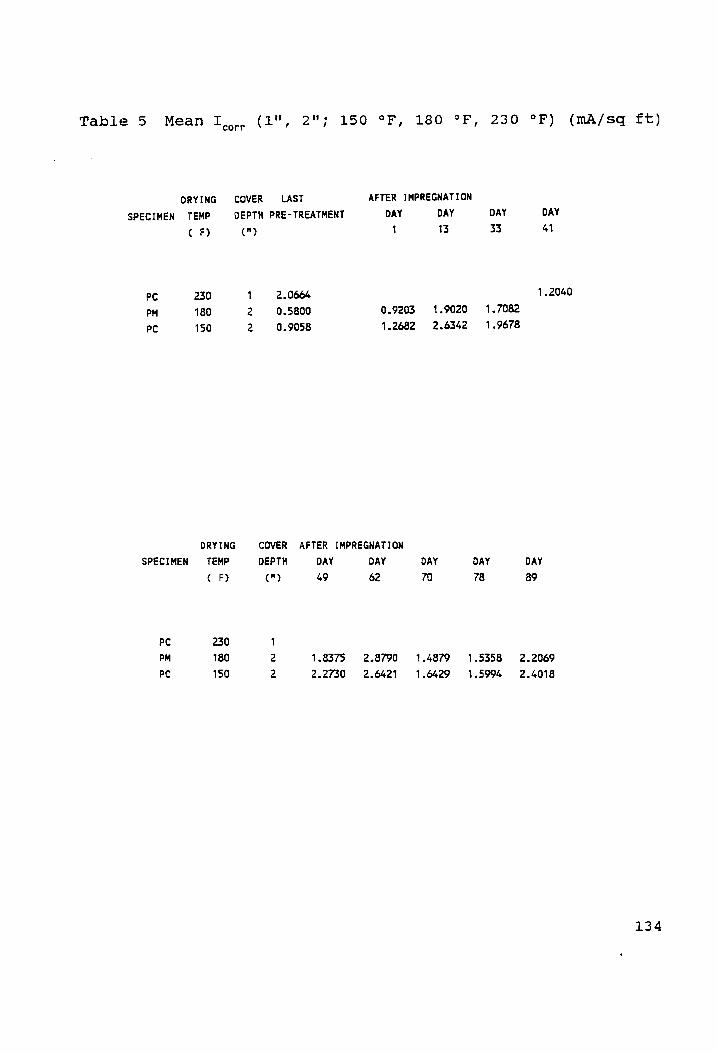
Table 5 Mean I (1", 2": 150 °F, 180 °F, 230 °F) (mA/sq ft) corr

DRYING COVER LAST AFTER IMPREGNAT ION

SPECIMEN TEMP DEPTH PRE-TREATMENT DAY DAY DAY DAY

( F) (") 1 13 33 41

PC 230 1 2.0664 1.2040

PM 180 2 0.5800 0.9203 1.9020 1.7082

PC 150 2 0.9058 1.2682 2.6342 1.9678

DRYING COVER AFTER IMPREGNATION

SPECIMEN TEMP DEPTH DAY DAY DAY DAY DAY

( F) c") 49 62 70 78 89

PC 230

PM 180 2 1.8375 2.8790 1.4879 1.5358 2.2069

PC 150 2 2.2730 2.6421 91.6429 1.5994 2.4018

134

" Table 5 Mean I,,,, (1",

DRYING SPECIMEN TEMP

( F)

PC 230 PM 180 PC 150

DRYING SPECIMEN TEMP

¢ F)

PC 230 PM 180 PC 150

2"; 150 °F, 180 °F, 230

(Contd. )

COVER AFTER IMPREGNATION DEPTH DAY DAY DAY

c") 105 125 141

1 0.4195 0.3690 0.3352 2 2

COVER AFTER IMPREGNATION DEPTH DAY DAY DAY

c") 154 162 170

1 0.3671 0.3347 0.3050 2 2

oF)

DAY

181

0.3300

(mA/sq ft)

135

6.0 FINDINGS AND CONCLUSIONS

6.1 Findings

The Cu-CuSO, Half-Cell proved to be an unreliable

instrument after active corrosion cells had been

successfully abated by the various treatment methods.

The three-electrode linear polarization device (3LP)

manufactured by Kenneth C. Clear, Inc. was sensitive to

ambient temperature.

It was confirmed that the major portion of the corrosion

cell is micro-cell in nature.

Reducing concrete drying temperature from 230 °F to 180 °F

resulted in drying time reduction by a factor of 2.5.

Concrete with structural damage impairs the effectiveness

of polymer impregnation as a corrosion abatement

technique.

Polymer molecules, being large organic molecules fill

voids in concrete selectively and there exists a lower

limit of void size which can be filled by the monomer.

Polymer impregnation of mortar cubes provided good

resistance against the ingress of chloride ions.

136

6.2 Conclusions

There was little difference in the effectiveness of the

five treatment methods used in this study. However, there

remained a possibility that treatments involving low slump

dense concrete overlay might be less effective as a

corrosion abatement technique.

For low corrosion rates of treated specimens, the cathode

to anode area in the corrosion cell have little influence

on the corrosion activity.

Pre-impregnation drying temperatures can be lowered to

180 °F at 4" below top rebar level at the time heaters

are turned off. Due to the thermal gradient, the

temperature at that depth would continue to rise to about

200 °F. The study on the mortar cubes yielded the

conclusion that optimum impregnation is achieved ata

drying temperature of about 200 °F.

137

7.0 RECOMMENDATIONS FOR FUTURE RESEARCH

The following are suggested areas for future studies. Some of

the recommendations stemmed from this research while others

were studies which could not be accommodated within the scope

of this project.

If a modified version of the 3LP device incorporating

temperature correction is not available in the market in the

near future, an experimental study could perhaps be undertaken

to develop an empirical temperature correction factor such

that all 3LP data taken at different temperatures could be

transformed to a base temperature. This would expand the use

of the 3LP device to all weather conditions.

A study on operator variability in the 3LP device could easily

be undertaken. Several operators would take readings with the

same instrument on the same specimens. The differences in

instrument readings would be tested for statistical

significance.

The exact cause of the failure of the Cu-CuSo, half-cell to

interpret corrosion rates after corrosion activity is stopped

should be investigated. This may lead to suitable

modifications so that the half-cell would be a more useful

tool.

Long term studies should be performed to investigate the

138

nature of corrosion activities long after treatment methods

had been applied. This would lead to the development of life-

cycle models for different bridge deck rehabilitation

techniques covered in the present study.

Other practical factors could be added to the study of

effectiveness of the treatment methods used in this study. Two

suggested factors are the influence of traffic volume and

major classes of vehicle loadings on the bridge decks.

139

APPENDIX A

DESIGN PARAMETERS

140

Table Al Mix Design - Specimens

Quantities per batch of specimens (SSD) in lb

Cement:

Water:

Coarse aggregate: Fine aggregate:

BATCH SLUMP # ()

1 2 1/4 2 1 3/4 3 3.1/4 4 2 1/2

42.64 16.96 72.54

109.54

141

Table A2 Compressive Strength - Specimens (psi)

mW

4850 5917 5556 5376

142

Table A3 Mix Design - Overlays

Quantities are in lb (OD)

LSDC LMC

Cement: 54.43 43.56 Water: 19.29 7.96

Latex: - 13.77 Coarse aggregate: 87.70 86.70 Fine aggregate: 87.96 97.07 AEA (Microair): 11.40 ml -

Total: 249.38 249.06

Slump: 0.25" 5.5" (after 5 min)

Air: 6.5 % 4 %

Bonding agent: Cement paste Latex paste

143

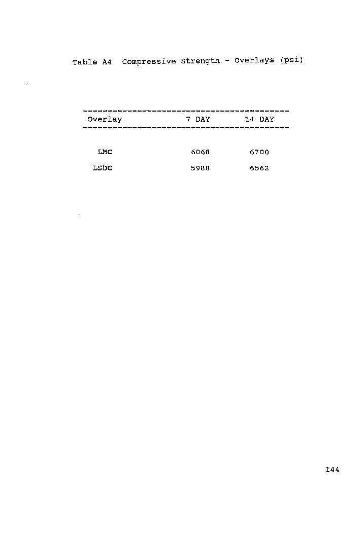
Table A4 Compressive Strength - Overlays (psi)

Overlay 7 DAY 14 DAY

LMC 6068 6700

LSDC 5988 6562

144

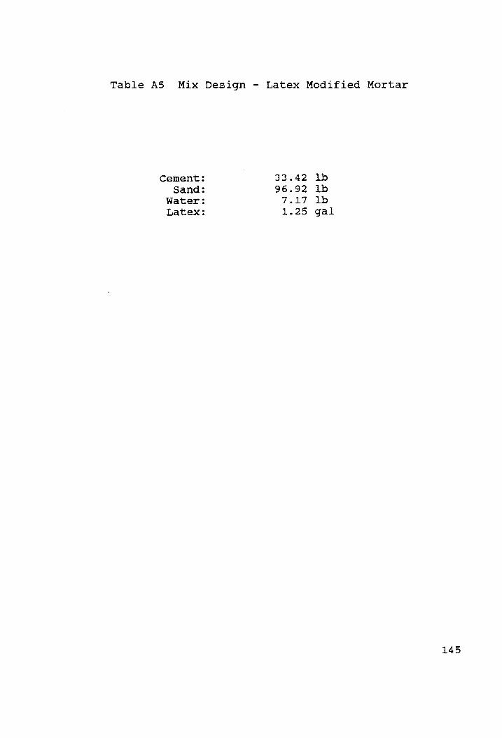
Table AS Mix Design - Latex Modified Mortar

Cement:

Sand: Water:

Latex:

33.42 96.92 7.17 1.25

lb Lb 1b gal

145

Table A6é Mix Design - Mortar Cubes

Quantities for six cubes ing

Portland cement (Type I): 500 Water (w/c=0.47): 235 Sand: 1380

146

Table A7 Compressive Strength of Air Dried Mortar Cubes (psi)

Cube # Strength

1A 5125 1B 4625 ic 3625

147

Table A8 Properties of Materials Used in the Specimens

(A) Coarse Aggregates

Unit weight:

Voids in dry rodded aggregate:

Bulk Specific Gravity (Ory):

Bulk Specific Gravity (SSD):

Apparent Specific Gravity:

Absorption:

(B) Fine Aggregates

Bulk Specific Gravity (Dry):

Bulk Specific Gravity (SSD):

Apparent Specific Gravity:

Absorption:

Fineness Modulus:

96.5 lb/cu ft

44.18 %

2.77 g/cc

2.78 g/cc

2.81 g/cc

0.57 %

2.61 g/cc

2.66 g/cc

2.66 g/cc

0.36 %

3.39

148

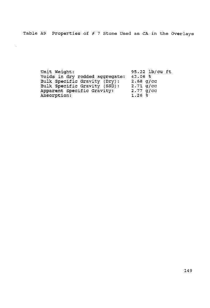
Table A9 Properties of # 7 Stone Used as CA in the Overlays

Unit Weight: Voids in dry rodded aggregate: Bulk Specific Gravity (Dry): Bulk Specific Gravity (SSD): Apparent Specific Gravity: Absorption:

95.22 lb/cu ft 43.06 % 2.68 g/cc 2.71 g/cc 2.77 g/cc 1.26 %

149

APPENDIX B

INSTRUMENT USE

-150

(1) Copper-Copper Sulfate Half-Cell

The half cell was used in accordance with the American Society

for Testing and Materials Standard C-876-87 [16].

The main components in this test are a Copper-Copper Sulfate

Half-Cell, two lengths of cables with alligator clips at one

end, a voltmeter, pieces of sponge and wetting agent. The

wetting agent used was common soap solution.

The cable connected to the positive terminal of the voltmeter

was hooked to the anode. The negative terminal was attached to

the half-cell. The voltmeter was adjusted such that it read

millivolts.

Three readings were taken per anode. Thus, a total of six

readings were taken for each specimen. The sponge pieces were

so cut that they were only a little bigger in size than the

half-cell cross section area. The sponge were moistened with

the wetting agent and placed on the concrete surface directly

over the anode. The three positions were the front, middle and

rear. The wetting of the concrete was for ensuring good

conductivity in the electrical circuit formed by placing the

half-cell on top of the wet sponge. The voltage readings were

taken after the display had stabilized within a_ few

millivolts. Normally this occurred within three minutes of

placing the half-cell on the sponge.

In taking half-cell readings as in the 3LP measurements, the

151

concrete was kept sufficiently wet throughout the length of

the measurement were taken.

(B) The Three Electrode Linear Polarization Device

The 3LP device (Model 3LP NBSI) is manufactured by Kenneth C.

Clear, Inc. The three electrodes are the corroding rebar

(anode), the counter electrode through which the counter-

potential is applied and a standard Cu-CuSo, half-cell.

The instrument imposes a known value of potential in a

direction contrary to that of the current in the corrosion

cell thereby polarizing the normal cell. The corresponding

value of the current is noted. This operation is repeated for

four values of potential. The counter potential used were 0,

4, 8 and 12 mV. The corresponding values of current (Topo)

were recorded in mA.

The Stern-Geary equation was employed which is:

Teorr = Lapp (8, * 8,)/{2-3 Ap (B, + B,)} (4)

where,

corr = COrrosion current in mA,

appt = Current corresponding to the counter potential in mA,

A@ = the counter potential in mv,

B. = anodic tafel slope = 150 mV/decade, and

B. = cathodic tafel slope = 250 mV/decade.

152

The values of the tafel slopes given above were obtained from

a large number of experimental data and were provided in the

3LP manual [17].

The corrosion current in mA/sq ft is given by the following

relation:

Toore = 14953.95 xX S/(K.B) (5)

where,

I = corrosion current in mA/sq ft, corr

S = Tapp / AG, obtained from above,

K corroding bar length in inches, and

B = bar number, as per ASTM specifications A-615.

In this study, K was 6.5" and B was 4.

In practice, the I values in mA/sq ft were computed using corr

an IBM-PC compatible software which is supplied with the 3LP

package. The current values corresponding to the four imposed

potential values and values of K and B were the input

parameters.

153

(C) The Specific Ion Probe

The ion probe manufactured by James Instruments, Inc. [18] was

used to obtain the chloride contents of selected specimens

before treatments as well as for the mortar cubes.

The manufacturers provided three standard solutions marked 1,

oo

2 and 3 of known chloride concentrations of 0.005 %, 0.05

and 0.5 %, respectively. Before testing the powdered concrete

samples (extraction procedure is described shortly), the probe

had to be calibrated against the standard solutions. The meter

was turned on and set in the "volt" mode. The meter displayed

readings in mV. The probe was inserted in standard solution 1

and the meter reading was noted after a period of three

minutes in which time the display had been allowed to

Stabilize. Similarly, the mV readings corresponding to

solutions 2 and 3 were obtained.

James Instruments, Inc. recommends the use of a semi-log graph

paper and plotting the mV readings against % Cl” in order to

get the calibration relation. In this study, however, a simple

linear regression was run to obtain the calibration equation

connecting mV with % Cl’.

The calibration had to be performed each time the meter was

turned on.

After the calibration was done, each sample was tested in the

following manner.

154

3 g of sample - weighed in a triple beam balance - was

introduced into a fixed volume of "chloride extraction

solution" provided with the ion probe package and shaken

vigorously for 15 seconds with the cap fixed tight. The probe

was then immersed in it and the mV reading was taken after a

period of three minutes. The reaction temperature was also

recorded by inserting a TC wire into the solution of the

extraction liquid and sample at the time the probe had been

immersed in it.

The mV reading was substituted in the calibration equation to

obtain the corresponding value of % Cl’. Corrections for

temperature and standardization to the standard potentiometric

titration method (AASHTO T-260-78) were done. Finally, the

chloride content in % Cl was converted to Cl in lb of

chloride per cubic yard of concrete.

The extraction equipment consisted of a power drill with a

hollow bit which had an orifice at the cutting edge, a tube

that led from the drill to a standard wet-dry shop vacuum, a

collection receptacle attached to the vacuum and ordinary

coffee filter paper. The drill unit had a frame such that the

depth of penetration could be adjusted.

The powdered sample was collected at the cutting edge of the

bit and sucked by the vacuum via the tube and collected ina

coffee filter placed in the collecting receptacle. The coffee

filter was folded and stored in small plastic containers until

155

the ion probe test.

More details can be found in the thesis by Steve Herald [19].

(D) The Resistivity Meter

Resistivity of the mortar cubes were found with a modified

soil resistivity meter. The two sets of cables in the meter

was soldered onto two circular metal surfaces which served as

the electrodes propagating the current through the cube. The

contact diameter was 1 square inch. From Ohm's Law, R = V/I

where, R = resistance in 2, V = potential in Volt and I =

current in Ampere.

R = pL/A, where p = resistivity in 2 inch, L = length in inch,

and A = cross section area in square inches. p, L and A can be

any compatible units.

Transposing, p = A.R/L

In centimeters, the above translated into:

p = (m X 2.54 X 2.54 X R)/(4 X 2.54 X 2)

Simplifying, p = 0.997 x R

The meter read resistance values in 2. However, since the

values of resistivity and resistance were nearly equal in this

particular experimental set up, the meter readings were

approximated.as resistivity values in cm.

Two small circular pieces were moistened, placed over the

contact area and the two contact areas were clamped tightly at

156

the center of two opposite sides of each cube. The dials were

adjusted until the null point was reached and the dialed value

was recorded. For each cube, three readings were taken across

the three pairs of sides and the mean value of resistivity

calculated.

157

APPENDIX C

EXPERIMENTAL DATA

158

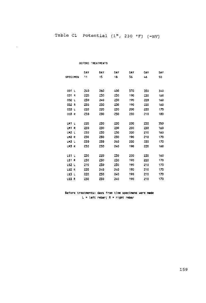
Table Cl Potential (1", 230 °F) (-mv)

BEFORE TREATMENTS

DAY DAY DAY DAY DAY DAY

SPECIMEN 11 15 18 36 46 50

cot L 240 260 400 370 350 340

coi R 220 230 230 190 230 160

co2 L 230 240 230 190 220 160

co2 R 230 230 230 190 220 160

Cos L 220 220 230 200 220 170

CO3 R 230 230 230 200 210 180

LMT L 220 230 230 200 230 350

LM1 R 230 230 230 200 230 160

LM2 L 230 230 230 200 210 160

LM2 R 230 230 230 190 210 170

LM3 L 230 230 240 200 220 170

LM3 R 230 230 240 190 220 160

LS7 L 230 220 230 200 220 160

LST R 230 230 230 190 220 170

Ls2 L 210 230 230 190 210 170

LS2 R 220 240 240 190 210 170

LS3 Lb 220 230 240 190 210 170

LS3 R 230 230 240 190 210 170

Before treatments: days from time specimens were made

L = left rebar: R = right rebar

159

Table Cl Potential (1", 230 °F) (-mV) (Contd.)

BEFORE TREATMENTS

DAY DAY DAY DAY DAY

SPECIMEN 116 123 141 155 214

col L 390 390 480 510 590

CO1 R 400 400 500 520 590

co2 L 370 370 480 410 550

co2 R 320 320 450 450 510

cCO3 L 340 340 400 410 540

co3 R 370 370 400 400 520

LM1 L 400 400 390 320 400

LM1 R 210 219 360 310 400

LM2 L 180 180 185 190 220

LM2 R 230 230 270 300 390

LM3 L 200 200 300 370 460

LM3 R 200 200 310 390 490

LST L 280 280 330 400 530

LS1 R 180 180 310 400 490

LS2 Lb 450 450 480 480 470

LS2 R 420 420 490 490 480

LS3 L 200 200 205 180 380

LS3 R 200 200 200 180 240

Before treatments: days from time specimens were made

L = left rebar; R = right rebar

160

Table Cl

SPECIMEN

PC1

PC1

PC2

PC2

PCS

PC3

PM1

PM1

PM2

PM2

PM3

PM3

PS1

PS4

PS2

PS2

PS3

PS3

NT

XY TF

wD

Te A

Tf AT

v

T- A

- ADAryar

Potential (1",

BEFORE TREATMENTS

DAY

11

220

220

220

220

230

220

230

220

220

220

230

230

230

240

230

230

230

230

DAY

15

240

230

230

230

230

240

230

240

220

230

240

230

230

230

240

240

230

240

DAY

18

230

240

230

240

240

230

240

230

240

230

240

230

230

230

230

240

230

240

230 oF)

DAY

36

200

180

190

180

190

190

190

190

190

190

200

190

190

190

190

200

190

190

(~mV)

DAY

46

210

210

220

220

210

210

210

220

210

210

210

210

210

210

220

220

210

210

Before treatments: days from time specimens were made

L = left rebar: R = right rebar

(Contd. )

DAY

50

180

160

150

150

160

160

160

160

170

160

180

170

160

160

160

170

170

170

161

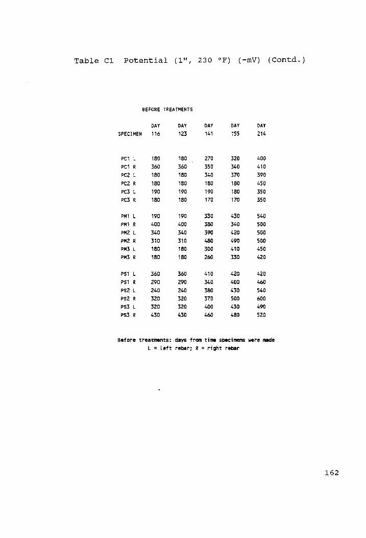
Table Cl Potential (1",

SPECIMEN

PC

PC4

PC2

PC2

PCS

PC3

PM1

PM4

PM2

PM2

PM3

PM3

PS1

PS1

PS2

PS2

PS3

PS3

A

TT

WF TF

AD

A

-

A

Tr AT

ATF

wae Ar

BEFORE TREATMENTS

DAY

116

180

360

180

180

190

180

190

400

340

310

180

180

360

290

240

320

320

430

DAY

123

180 360

180

180

190

180

190

400

340

310

180

180

360

290

240

320

320

430

230

DAY

141

270

350

340

180

190

170

330

380

390

480

300

260

410

340

380

370

400

460

oF) (-mV)

DAY DAY

155 214

320 400

340 410

370 390

180 450

180 350

170 350

430 540

340 500

420 500

490 500

410 450

330 420

420 420

400 460

430 540

500 600

430 490

480 520

(Contd. )

Before treatments: days from time specimens were made

L = left rebar; R = right rebar

162

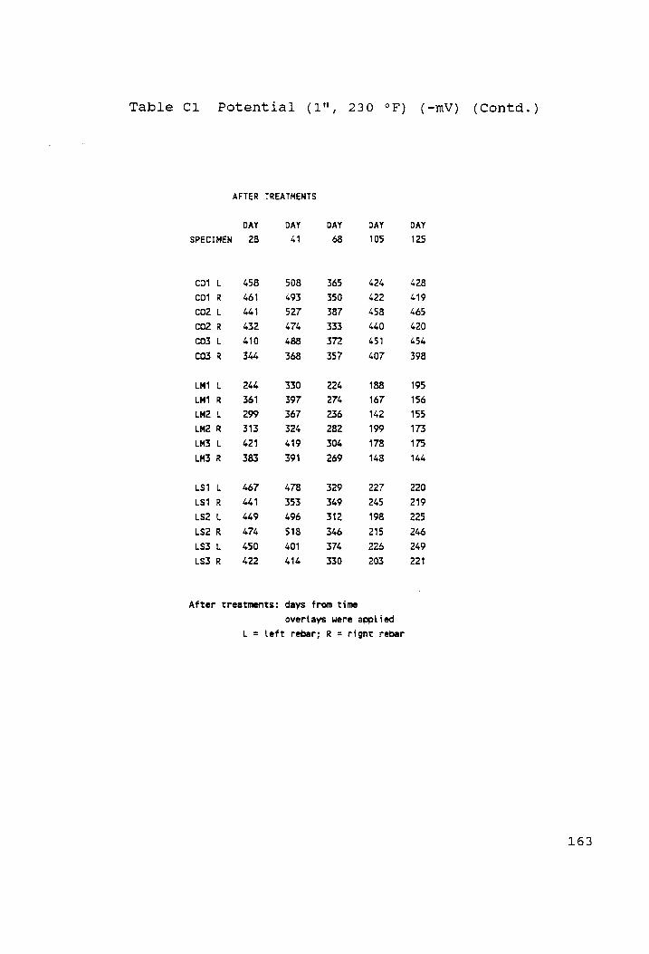
Table Cl

SPECIMEN

co1

cot

co2

co2

co3

CO3

LM1

LMT

LM2

LM2

LM3

LM3

LS1

LSi

Ls2

Ls2

LS$3

Ls3

Potential (1",

ya - Rrra

rT A

-

A Ta

rT Aer DT

WD

AFTER

DAY

28

458

461

441

432

410

344

244

361

299

313

421

383

467

441

449

474

450

422

TREATMENTS

DAY

41

508

493

527

474

488

368

330

397

367

324

419

391

478

353

496

518

401

414

DAY

365

350

387

333

372

357

224

274

236

282

304

269

329

349

312

346

374

330

230 °F)

DAY

105

424

422

458

440

451

407

188

167

142

178

148

227

245

198

215

226

203

After treatments: days from time

overlays were applied

left rebar; 8 = L = right rebar

(~mvV)

DAY

125

428

419

465

420

454

398

195

156

155

173

175

144

220

219

225

246

249

221

(Contd. )

163

Table Cl Potential (1",

AFTER TREATMENTS

SPECIMEN

CO1

co1

co2

co2

Co3

CO3

LM

LM1

LM2

LM2

LM3

LM3

Ls1

LS1

LS2

LS2

Ls3

LS3

After

a

-

A

T-

wD

nT

DD

T- AT

aT

DT

2

DAY

141

501

500

555

526

528

503

248

206

194

223

239

240

300

314

291

317

314.

293

DAY

154

525

532

570

535

537

517

e777

217

296

211

306

239

284

296

276

293

279

281

DAY

162

496

500

552

524

527

506

249

17

232

192

282

212

268

ev?

237

278

270

257

230 °F)

DAY

170

486

491

531

511

506

495

242

159

264

205

273

201

210

249

213

227

256

264

treatments: days from time

overlays were applied

L left rebar: R right rebar

(-mvV)

DAY

181

500

505

556

528

538

512

263

193

281

210

306

281

251

289

266

314

268

263

(Contd. )

164

Table C1 Potential (1",

AFTER TREATMENTS

DAY DAY DAY

SPECIMEN 28 41 68

Pet L431 446306 PCT R «6-313 495 348 Pe2L 41S 491 323 pc2R 864510 425 252 PCS L060 256 321140 PCS R 406 470 297

PMI L 86460 5223579 PMI R 4465 484 373 PM2 L455 5310377 PM2 R 86-378 533 379 PMS L488 S16 396 PMS R 86499 5350355

PS1L 6520 549 45 Pst R 515 9551 412 Ps2L 509 480 344 PS2R 452 568 402 PSSL S270 536 4B PSSR 481 738 397

230 °F)

DAY

105

231

234

172

147

142

171

365

332

373

359

396

349

388

369

437

390

361

379

After treatments: days from time

overlays were applied

L = left rebar; R = right rebar

(-mV)

DAY

125

228

161

138

112

167

343

377

368

319

358

325

370

340

441

373

347

353

(Contd. )

165

Table Cl Potential (1",

AFTER TREATMENTS

DAY

SPECIMEN 141

PCt

PC1

PC2

PC2

PCS

pcs

PM1

PM‘

PM2

PM2

PMS

PM3

PS$1

PS1

PS2

PS2

PS3

PS3

After

292

306

318

235

206

275 A

—

A

~~ wT

395

426

410

376

aA TfwAar

A

eT

38

394

378

468

381

400 Ra

~ KHOA

treatments: days from time

overtays were applied

L = left rebar: R

DAY

154

329

327

261

234

288

312

378

358

391

378

451

377

385

370

351

434

361

374

DAY

162

310

290

214

216

221

255

349

329

368

361

420

346

361

350

354

413

354

366

230

DAY

170

241

250

303

209

215

249

338

347

358

355

394

328

349

329

320

395

348

350

oF)

DAY

181

275

281

283

226

223

251

352

362

369

359

420

355

343

355

367

436

383

371

right rebar

(—mvV) (Contd. )

166

Table c2 I (1", 230 °F) (mA/sq ft) corr

BEFORE TREATMENTS AFTER TREATMENTS

DAY DAY DAY DAY DAY

SPECIMEN 179 214 41 105 125

col Lk 9.1601 9.2421 27.1644 19.0621 18.8822

cO1 R 8.9877 9.7140 26.2183 25.2179 27.0637

co2 & 8.1091 8.5654 12.7388 15.0019 14.2436

cO2 R 5.9987 6.1685 4.7665 6.2312 6.5437

co3 L 8.2721 9.9156 13.8625 19.8912 20.2999

co3 R 7.3167 7.3590 6.7148 8.3167 8.0161

LM1 L 1.8823 1.9104 0.9705 0.2167 0.2099

LM1 R 1.8767 1.9112 0.6873 0.1922 0.1811

LM2 Lb 0.5987 0.6122 1.3559 0.4167 0.2761

LM2 R 1.7169 1.7298 1.8419 0.3354 0.4097

LM3 L 2.0492 2.1415 2.8728 0.4267 0.4112

LM3 R 2.2328 2.2784 3.2122 0.9177 0.4543

LST L 5.8791 6.9107 3.1949 0.5767 0.4731

LS1 R 2.7654 2.8874 1.7729 0.8798 0.4601

L$2 L 2.0761 2.1528 7.1161 2.4875 2.8297

LS2 R 2.0692 2.2006 9.6711 4.3495 3.5803

LS3 L 1.6954 1.8769 3.88946 2.3624 2.3164

LS3 R 0.8226 0.8905 2.8383 0.5837 0.6182

Before treatments: days from time specimens were made

After treatments: days from time

overlays were applied

L = left rebar; R = right rebar

167

Table C2

SPECIMEN

co1

C01

co2

co2

co3

LM1

LM1

LM2

LM2

LS1

LSs1

LS2

Ls2

LS3

LS3

A

-— B®

—-— 2

rT ya

T-

FR FAT

A TAT

wT

I corr

(1", 230 °F)

AFTER TREATMENTS

DAY

141

20.0961

22.9245

17.5728

7.8017

18.7165

12.1319

0.1654

0.1482

0.2144

0.3913

0.4359

0.4057

0.9121

0.9826

0.6831

3.6929

1.9206

0.6833

DAY

154

24.8868

30.4701

19.0949

12.0988

18.8431

16.9729

0.2072

0.1913

0.3093

0.3999

0.5942

0.5956

0.7279

1.0473

3.5836

5.2511

1.7666

0.6042

DAY

162

22.5303

27.2562

18.9985

10.1365

22.7547

14.5331

0.2359

0.1771

0.2302

0.2892

0.4258

0.5913

0.9308

0.8718

3.3851

4.4079

1.8515

0.7021

After treatments: days from time

overtays were applied

L = left rebar: R = right

(mA/sq ft)

DAY DAY

170 181

25.1961 32.7229

26.9354 40.3721

20.6054 32.1389

11.4975 11.8097

20.0012 27.3928

12.5606 20.3824

0.2705 0.2777

0.2101 0.1913

0.1913 0.2892

0.3999 0.3971

0.5193 0.4661

0.4934 0.5107

0.6833 0.7136

0.8028 0.7625

3.3549 3.5922

5.3618 5.1719

2.2529 2.0991

0.7279 0.7423

rebar

(Contd. )

168

Table C2

SPECIMEN

PC

PCt

PC2

PC2

PCS

PCS

PM1

PM1

PM2

PM2

PMS

PM3

PS1

PS1

PS2

PS2

PS3

PS3

Before treatments: days from time specimens were made

After treatments: days from time

nT

DT

wT

AT

RTF fT

A

T-—

2A Tr

FT

I corr (1",

BEFORE TREATMENTS

DAY

179

2.0006

1.7762

1.9762

2.5793

1.0292

0.9981

7.1792

2.0788

3.2791

10.0062

1.5421

1.4466

1.7654

1.9862

7.4293

9.7214

2.6609

4.9781

DAY

214

2.0241

1.8803

1.9986

2.7761

1.8768

1.8423

8.4489

2.2847

3.7601

12.2651

1.7441

1.4479

1.9287

2.0671

7.6698

10.0161

2.6752

5.1917

230 °F) (mA/sq ft) (Contd.)

AFTER TREATMENTS

DAY

41

1.7657

2.4372

0.5924

0.4687

0.8066

1.1531

4.6501

3.9024

3.7988

5.7328

5.0009

7.7314

3.8075

3.6551

5.0584

6.4115

6.5308

7.7933

overlays were applied

L = left rebar: R = right rebar

DAY

105

0.3806

0.7791

0.1987

0.3688

0.4207

0.3692

1.8045

1.2523

1.3386

1.5931

1.9727

3.2761

1.3631

1.0482

4.3122

3.9455

1.6881

2.8887

DAY

125

0.4687

0.6182

0.2559

0.3767

0.2847

0.2099

2.1395

0.4328

1.5284

1.4177

1.9037

2.6169

1.6191

1.4709

5.6594

5.2266

3.0569

3.9699

169

Table C2

SPECIMEN

PC’

PC1

PC2

PC2

PCS

PC3

PM1

PM1

PM2

PM2

PM3

PMS

PS1

PS1

PS2

PS2

PS3

PS3

a renAarar

aT

WAT Ae

7m

DT

DT

I corr

(1", 230 °F)

AFTER TREATMENTS

DAY

141

0.3871

0.5999

0.2633

0.4287

0.1755

0.1568

1.8055

0.5467

1.6832

0.9251

2.6183

3.8124

1.8271

1.5163

1.9134

4.9575

3.1103

4.2756

DAY

154

0.4244

0.7668

0.1281

0.3985

0.2187

0.2661

2.0745

0.9768

1.9393

2.4385

2.9218

5.0107

2.1392

1.6645

1.9206

5.6826

4.5576

5.3056

DAY

162

0.4776

0.5697

0.2388

0.3654

0.1654

0.1913

1.7121

1.3264

1.4631

1.9968

2.5349

3.0873

2.4428

1.3739

1.8645

4.3188

3.3065

4.5086

After treatments: days from time

overlays were appl ied

L = left rebar; R

(mA/sq ft)

DAY DAY

170 181

0.3856 0.3323

0.5611 0.56488

0.2316 0.2676

0.2287 0.3871

0.1539 0.1511

0.2691 0.1928

1.9004 1.8918

0.5352 0.4776

1.9047 1.9321

1.9695 2.2903

2.7781 2.4284

4.2857 4.2051

1.8213 1.2201

1.9637 1.7163

2.7463 1.6127

5.5459 5.2726

3.4931 4.6295

3.0197 4.4036

= right rebar

(Contd. )

170

Table C3 Macro L,,,, (1", 230 °F) (mA)

BEFORE TREATMENTS AFTER TREATMENTS

DAY DAY DAY DAY

SPECIMEN 141 155 28 76

co1 L -0.0371 -0.041 0.05 -0.009

Coi R -0.0683 -0.076 0.07 -0.019

co2 L 0.0071 0.071 0.09 NA

co2 R -0.0581 -9.055 0.06 -0.019

co3 & -0.0542 -0.057 0.09 0

COS R -0.0251 -0.021 0.08 -0.023

LM1 L 0.0201 0.011 “0.01 -0.001

LMT R 0.0071 0.003 0.03 0

LM2 L NA 0 -0.03 -0.001

LM2 R NA 0.001 0.01 -d.002

LM3 Lb NA -0.006 0.06 -0.002

LM3 R NA 0.015 0.1% -0.006

LS1 L NA -0.025 0.22 -0.011

LS1 R NA -0.017 0.11 0

LS2 L 0.0501 0.041 0.15 -0.037

LS2 R 0.9102 0.099 0.16 -0.035

LS3 L NA ) 0.18 -0.001

LS3 R NA 0 0.04 -0.003

Before treatments: days from time specimens were made

After treatments: days from time

overlays were applied

L = left rebar; R = right rebar

171

Table C3 Macro I corr

AFTER TREATMENTS

DAY

SPECIMEN 141

co1

co1

co2

co2

co3

co3

LM1

LM1

LM2

LM2

LM3

LM3

LS

LS1

Ls2

LS2

LS3

LS3

After

-0.025

-0.046

-0.097

-0.048

-0.041

-0.006 a

rr

DFT

we

Ar

FD - 2

CT

oo

0 2 &

-0.002

-0.007

-0.001

-0.023

-0.028

-0.001

-0.003 a

7-— AT

AT

treatments:

L = left

DAY

154

-0.034

-0.065

-0.066

-0.058

-0.059

-0.061

0.003

0.006

-0.002

-0.007

-0.001

-0.017

-0.023

-0.001

-0.002

(1",

DAY

162

-0.032

-0.065

-0.131

-0.054

-0.069

-0.065

0.001

0.002

0.012

-0.001

-0.005

-0.001

-0.011

-0.018

-0.002

days from time

overlays were applied

230 °F)

DAY

170

-0.036

-0.071

70.064

-0.056

-0.092

-0.068

0.001

0.0001

0.011

0.001

-0.004

-0.001

-0.012

-0.015

-0.001

-0.002

rebar; R = right rebar

(mA )

DAY

181

-0.043

-0.081

-0.152

-0.062

-0.128

-0.081

0.002

0.009

0.016

0.011

-0.004

-0.002

-0.003

0.026

-0.001

-0.002

(Contd. )

172

Table C3 Macro I (1", 230 °F) (mA) (Contd.) corr

BEFORE TREATMENTS AFTER TREATMENTS

DAY DAY DAY DAY

SPECIMEN 141 155 28 76

PCT L NA 0.006 -0.03 -0.001

PC1 R 0.0101 0.007 0.04 0.002

PC2 L NA 0.021 -0.01 -0.001

PC2 R NA Q -0.03 -0.021

PCS L NA 0 0.01 0

PC3 R NA 0 -0.01 0.001

PMT L NA -0.032 0.18 -0.042

PM1 R 0.0151 0 0.06 -0.007

PM2 L -0.0291 -0.028 0.17 -0.031

PM2 R -0.0351 -0.026 0.44 -0.041

PM3 L NA 0.026 0.07 -0.009

PM3 R NA 0.011 0.21 NA

Psi L -0.0281 -0.046 0.27 -0.054

PS1 R NA -0.024 0.15 -0.035

Ps2 L NA -0.039 0.32 0

PS2 R -0.0231 -0.024 0.31 0

PS3 LL -0.0392 -0.039 0.13 -0.032

PS3 R -0.0582 -0.049 0.24 -0.058

Before treatments: days from time specimens were made

After treatments: days from time

overlays were applied

L = left rebar: R = right rebar

173

Table C3 Macro I (1", 230 corr

AFTER TREATMENTS

DAY DAY DAY DAY

SPECIMEN 141 154 162 170

PC1

PC1

PC2

PC2

PC3

PCS

PM

PM1

PM2

PM2

PM3

PMS

PS1

PS1

PS2

PS2

PS3

PS3

After

L “0.004 -0.014 -0.007 -0.004

R -0.005 -0.008 -0.006 -0.008

L 0 60.005 0 0

R -0.003 -0.004 -0.002 -0.001

L 0 -0.001 0 0

R 0 0 0 0

L -0.031 -0.027 -0.019 -0.021

R 0 -0.006 -0.003 0

L -0.024 -0.018 -0.013 -0.013

R -0.056 -0.027 -0.008 -0.011

L 0.012 -0.003 -0.007 -0.011

R -0.019 -0.018 -0.015 -0.019

L -0.038 -0.021 -0.016 -0.016

R “0.032 -0.026 -0.021 -0.022

L -0.137 -0.141 -0.005 -0.096

R -0.009 -0.061 -0.036 -0.041

L -0.012 0.019 0.028 0.038

R -0.037 -0.038 -0.024 -0.021

treatments: days from time

overlays were applied

L = left rebar; R = right rebar

°F) (mA)

DAY

181

-0.004

-0.008

-0.002

-0.019

-0.008

-0.012

-0.009

-0.016

-0.019

-0.015

-0.021

-0.085

-0.052

0.071

-0.017

(Contd. )

174

Table C4

(A) 1" cover, 230 F

BEFORE TREATMENTS DEPTH

SPECIMEN (")

CO1 0-1/2 1/2-1

1-1 1/2 1-2

1 1/2-2

CO3 0-1/2 1/2-1

1-1 1/2 1 1/2-2

LS3 0-1/2 1/2-1

1-1 1/2 1 1/2-2

Before treatments:

DAY 71

17.01 NA NA 1.04

NA

12.21 2.82 0.69 0.59

16.92 11.97 2.31 0.79

days from time specimens were made

DAY 190

19.38 12.91 8.03

NA 1.74

19.07 14.48 3.38 1.01

19.37 14.17 3.86 1.15

Chloride Content of Selected Specimens (1b/yd)

175

Table C4 Chloride Content of Selected Specimens (1b/yd?)

(Contd. )

(B) 2" cover, 180 F

SPECIMEN DEPTH (")

PM1 0-1/2 1/2-1

1-1 1/2 1 1/2-2 2-2 1/2 2 1/2-3

PM2 0-1/2 1/2-1

1-1 1/2 1 1/2-2 2-2 1/2 2 1/2-3

Before treatment: days from time specimens were made

BEFORE TREATMENT

DAY 154

19.71 8.84 1.74 1.12 0.97 1.01

19.96 7.34 1.51 1.44 1.28 1.23

176

Table C5

co

LS PC PM PS

Change in Micro I

DAY 144

13.7998 0.3515 1.4257 0.1204 1.8357 4.0258

corr over Time (1",

(mA/sq ft)

POST-TREATMENT DAY 147

20.9234 0.3194 1.8659 0.0949 1.6357 4.1931

DAY 149

21.4600 0.2815 1.6938 0.0969 1.7503 3.9150

230 oF)

177

Table C6

CO

LS PC PM PS

MICRO

13.7998 0.3515 1.4257 0.1204 1.8357 4.0258

Micro, Macro & Mixed I

MACRO

0.7663 0.0000 0.1457 0.0188 0.3150 0.8791

corr (1",

MIXED

18.7951 0.2719 1.1719 0.2753 2.0357 2.2836

230 oF) (mA/sq ft)

178

Table C7 Mixed I for Different C/A (1", 230 °F) (mA/sq ft) corr

C/A C/A C/A C/A 1 2 3 4

co 17.468 14.286 14.096 18.044 LM 0.369 0.315 0.527 0.454 LS 1.849 1.786 2.474 2.193 PC 0.627 0.395 0.531 0.486 PM 2.169 1.761 3.271 2.969 PS 3.761 3.583 4.114 3.852

179

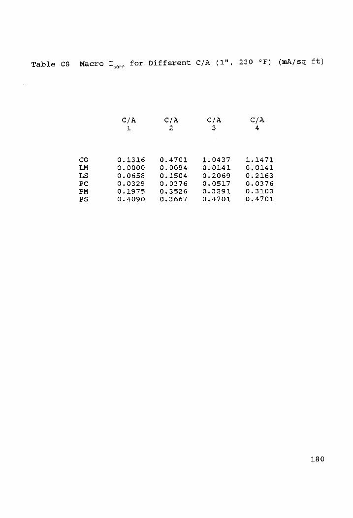
Table C8 Macro I

co

LS PC PM PS

for Different C/A (1", corr

C/A

0.1316 0.0000 0.0658 0.0329 0.1975 0.4090

C/A 2

0.4701 0.0094

0.1504 0.0376 0.3526 0.3667

C/A 3

1.0437 0.0141 0.2069 0.0517 0.3291 0.4701

230 oF)

C/A

1.1471 0.0141 0.2163 0.0376 0.3103 0.4701

(mA/sq ft)

180

Table C9 Potential (2", 4%"; 150 °F, 180 °F)

COVER DRYING BEFORE IMPREGNATION

SPECIMEN DEPTH TEMP DAY DAY DAY DAY

(") ( F) 10 28 98 186

Pc2 L 2 150 150 160 160

PC2 R 2 150 150 160 150

POS L 2 150 150 160 160

PCS R 2 150 160 160 160

PC2 L 3/4 150 454

PC2 R 3/4 150 418

PCS L 3/4 150 481

PC3 R 3/4 150 452

PM1 L 2 180 150 160 160

PM1 R 2 180 140 160 160

PM2 L 2 180 160 170 150

PM2 R 2 180 160 160 160

PM1 L 3/4 180 460

PM1 R 3/4 180 476

PM2 L 3/4 180 466

PM2 R 3/4 180 335

cot L 2 160 150 160

CO1 R 2 - 170 160 160

co2 L 2 - 150 160 160

co2 R 2 - 150 160 160

col t 3/4 - 447

Cot R 3/4 - 427

co2 L 3/4 - 417

co2 R 3/4 418

Before impregnation: days from time specimens were made

L = left rebar; R = right rebar

(-mvV)

181

Table c9 Potential

COVER SPECIMEN DEPTH

()

PC2 L 2 PC2 R 2 Pc3 L 2 PC3 R 2 PC2 L 3/4 PC2 R 3/4 PC3 L 3/4 PCS R 3/6

PM1 L 2 PM1 R 2 PM2 L 2 PM2 R 2 PM1 L 3/4 PM1.R 3/4 PM2 L 3/4 PM2 R 3/4

coi L 2 CO1 R 2 co2 L 2 CO2 R 2 coi L 3/6 CO1.R 3/4 co2 L 3/4 CO2 R 3/4

Before impregnation: days from time specimens were made

(2",

150

150

150

150

150

150

150

150

180

180

180

180

180

180

180

180

LH. a

DAY

199

180

180

190

200

380

170

190

190

160

170

190

180

150

DAY

370

156

225

355

125

352

360

205

180

285

301

320

318

oF,

ORYING BEFORE IMPREGNATION

TEMP

( FY

180

AFTER I[MPREGNATION

DAY

1

241

340

528

232

568

563

720

698

462

502

NA

NA

654

661

591

509

NA

NA

NA

NA

NA

NA

NA

NA

After impregnation: days from time of impregnation

L = left rebar; R = right rebar

oF)

DAY

13

262

338

510

310

487

427

500

496

460

489

327

205

411

462

421

441

290

300

205

221

397

367

354

(-mvV)

DAY

33

264

242

389

268

413

424

469

470

355

427

318

194

422

408

418

429

171

184

189

103

407

373

388

361

(Contd. )

182

Table C9 Potential (2", 4%"; 150 °F,

COVER DRYING AFTER IMPREGNATION SPECIMEN DEPTH TEMP DAY DAY DAY

cH) CF) 49 62 70

PC2 L 2 150 356 345 317 PC2 R 2 150 377 364 332 PC3 L 2 150 355 419 374 PC3 R 2 150 301 383 361 PC2 L 3/4 150 496 506 505 PC2 R 3/4 150 532 530 504 PC3 L 3/4 150 525 518 486 PC3 R 3/4 150 504 505 459

PM1 L 2 180 663 438 387 PM1 R 2 180 501 473 428 PM2 L 2 180 301 432 416 PM2 R 2 180 340 389 297 PMT L 3/4 180 452 530 475 PM1 R 3/4 180 478 550 516 PM2 L 3/4 180 499 571 527 PM2 R 3/6 180 495 518 535

col L 2 - 268 213 194 COI R 2 - 312 280 257 Co2 L 2 - 323 258 282

CO2 R 2 - 337 306 313 cot L 3/4 - 493 512 463 COI R 3/4 - 483 489 478 CO2 L 3/4 . 457 459 437 cCO2 R 3/4 - 455 486 450

After impregnation: days from time of impregnation

L = left rebar: R right rebar

180 °F)

DAY

78

319

330

380

360

517

522

300

485

370

429

410

301

503

536

550

542

167

232

298

325

501

496

494

487

(-mvV)

DAY

89

331

354

377

359

560

558

528

518

390

447

421

360

520

548

583

572

188

264

238

337

521

550

538

551

(Contd. )

183

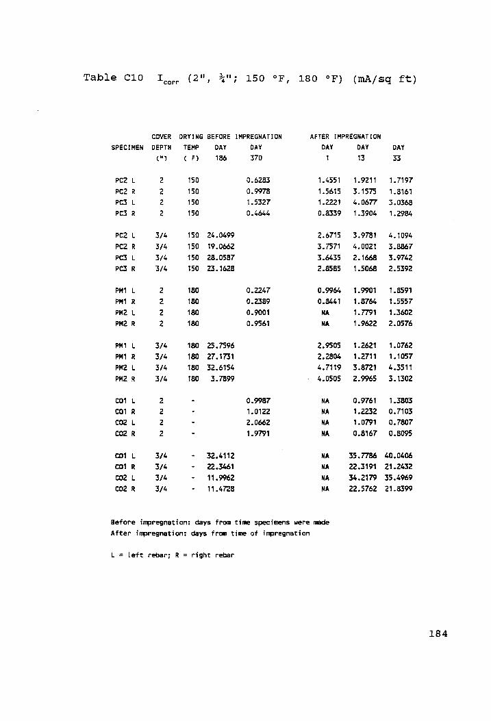
Table c10 I

PC2

PC2

PC3

PCS

PC2

PC2

PC3

PCS

PM1

PM1

PM2

PM2

PM1

PM1

PM2

PM2

cot

co1

co2

co2

co1

co1

co2

corr (2", 4"; 150 °F,

COVER ORYING BEFORE

SPECIMEN OEPTH TEMP

(") € F)

L 2 150

R 2 150

L 2 150

R 2 150

L 3/4 150

R 3/4 150

L 3/4 150

R 3/4 150

L 2 180

R 2 180

L 2 180

R 2 180

L 3/4 180

R 3/4 180

L 3/4 180

R 3/4 180

L 2 -

R 2 -

L 2 -

R 2 -

L 3/4 -

R 3/4 -

L 3/4 -

R 3/4 -

Before impregnation:

co2

DAY

186

24.0499

19.0662

28.0587

23.1628

25.7596

27.1731

32.6154

3.7899

32.4112

22.3461

11.9962

11.4728

IMPREGNATION

DAY

370

0.6283

0.9978

1.5327

0.4644

0.2247

0.2389

0.9001

0.9561

0.9987

1.0122

2.0662

1.9791

180 °F)

AFTER IMPREGNATION

DAY 4

1.4551

1.5615

1.2221

0.8339

2.6715

3.7571

3.6435

2.8585

0.9964

0.8441

NA

NA

2.9505

2.2804

4.7119

4.0505

NA

NA

NA

NA

NA

NA

NA

NA

days from time specimens were made

After impregnation: days from time of impregnation

L left rebar; R = right rebar

(mA/sq ft)

DAY

13

1.9211

3.1575

4.0677

1.3904

3.9781

4.0021

2.1668

1.5068

1.9901

1.8764

1.7791

1.9622

1.2621

1.2711

3.8721

2.9965

0.9761

1.2232

1.0791

0.8167

35.7786

22.3191

34.2179

22.5762

DAY

33

1.7197

1.8161

3.0368

1.2984

4.1094

3.8867

3.9742

2.5392

1.8591

1.5557

1.3602

2.0576

1.0762

1.1057

4.3511

3.1302

1.3803

0.7103

0.7807

0.8095

40.0406

21.2432

35.4969

21.8399

184

Table C10 I... (2", 4"; 150 °F, 180 °F) (mA/sq ft) (Contd. )

COVER DRYING AFTER IMPREGNATION

SPECIMEN OEPTH TEMP DAY DAY DAY DAY DAY

(") ( F) 49 62 70 78 89

PC2 L 2 150 3.1837 2.1881 1.8127 1.8285 2.9549

PC2 R 2 150 2.7161 2.3911 1.9019 1.9954 2.5406

PC3 L 2 150 2.0846 3.6081 1.4444 1.3481 2.3565

PC3 R 2 150 1.1077 2.3809 31.4127 1.2257 1.7551

PC2 L 3/4 150 6.7529 9.1856 9.3626 15.4825 12.8699

PC2 R 3/4 150 8.3224 14.7819 9.6934 17.1973 13.2958

PC3 L 3/4 150 3.7534 6.7256 3.9663 8.3066 10.1121

PCS R 3/4 150 1.7321 5.5401 2.8816 6.6393 9.2705

PM1 L 2 180 1.9263 2.7952 1.6041 1.5481 2.0385

PM1 R 2 180 2.3493 4.4741 2.2673 1.9652 3.2701

PM2 L 2 180 1.1381 1.5393 1.1092 1.3696 1.4343

PM2 R 2 180 1.9364 2.7075 0.9711 1.2602 2.0846

PMT L 3/4 180 1.9896 14.3474 4.8956 8.7281 9.6114

PM1 R 3/4 180 1.7192 14.7387 4.3418 6.3731 4.9992

PM2 L 3/4 180 4.5374 30.5506 10.7422 27.7798 27.1396

PM2 R 3/4 180 2.1939 17.7901 5.9027 17.6908 11.6543

CO1 L 2 - 2.3637 1.2027 1.1883 1.4357 1.0804

coi R 2 - 1.7407 1.3711 «1.1998 1.3178 1.0775

co2 L 2 - 1.28971 1.0185 1.1711 1.2746 0.6301

cO2 R 2 - 1.7997 1.7781 1.8314 1.4789 1.9652

coi L 3/4 - 43.9543 54.2045 43.0393 50.6727 89.9644

C01 R 3/4 - 31.6986 47.6242 36.2821 51.0295 72.6908

coe L 3/4 - 45.9583 47.1207 41.7604 50.0181 94.4514

co2 R 3/4 - 40.9447 53.8002 41.0799 60.9214 99.3371

After impregnation: days from time of impregnation

L = left rebar; R = right rebar

185

Table C11 Macro I corr

PC2 PC2 PC3 PC3 PC2 PC2 PC3 PC3

PM1 PM1 PM2 PM2 PM1 PM1 PM2 PM2

col col CcO2 CO2 col col C02 CO2

After impregnation:

L

POABerDrAr

ADAranrwdrwne

ADArwerwaran

left rebar; R =

(")

3/4 3/4 3/4 3/4

TEMP ( F)

150 150 150 150 150 150 150 150

180 180 180 180 180 180 180 180

days from time of impregnation

(2", %"; 150

DAY 49

0.029 -0.053 -0.053 0.044 0.038

-0.042 0.001 0.021

0.079 0.041

0 -0.034 0.054 0.031

0 0.025

0.149 -0.201 -0.006 “0.035 0.006 0.018

0 -0.018

right rebar

°F, 180

COVER DRYING AFTER IMPREGNATION SPECIMEN DEPTH DAY

62

0.045 -0.054

0 0.041 0.033

-0.059 -0.016 0.071

0.046 0.031

0 0.296 0.041

-0.019 -0.129 -0.215

0.002 0.016

0 -0.025 0.099

-0.232 0.027

-0.119

oF)

DAY 70

0.038 “0.041

0.032 0.017

-0.076

-0.022 0.049

0.029 0.015

0.097 0.041

-0.033 -0.006 -0.222

0.001 0.011

“0.025 0.175

-0.134 0.096 0.018

(mA )

186

Table C11 Macro I...

COVER

SPECIMEN DEPTH

(")

PC2 L 2

PC2 R 2

PC3 L 2

PC3 R 2

Pc2 L 3/4

PC2 R 3/4

PC3 L 3/4

PC3 R 3/4

PM1 L 2

PM1 R 2

PM2 L 2

PM2 R 2

PM1 L 3/4

PM1 R 3/4

PM2 L 3/4

PM2 R 3/4

col L 2

co1 R 2

co2 L 2

CcO2 R 2

coi L 3/4

CcO1l R 3/4

co2 L 3/4

co2 R 3/4

After impregnation: days from time of

L=

xu ° f

150 150 150 150 150 150 150 150

180 180 180 180 180 180 180 180

oF, 180

DAY 78

0.036 -0.043

0 0.033

-0.001 -0.119 -0.049 0.031

0.031 0.021

0 0.098 0.057

-0.015 -0.108 -0.083

0.002 0.011

-0.001 -0.027 0.111

-0.133 0.039 0.011

left rebar; R = right rebar

oF)

DRYING AFTER IMPREGNATION TEMP

( F) DAY 89

0.037 -0.043

9) 0.029

-0.028 -0.125 -0.077 0.001

0.027 0.021

0 0.037 0.056 0.013

~Q.111 -0.067

0 0.009

0 -0.035 0.141

-0.081 0.058

-0.011

impregnation

(mA ) (Contd. )

187

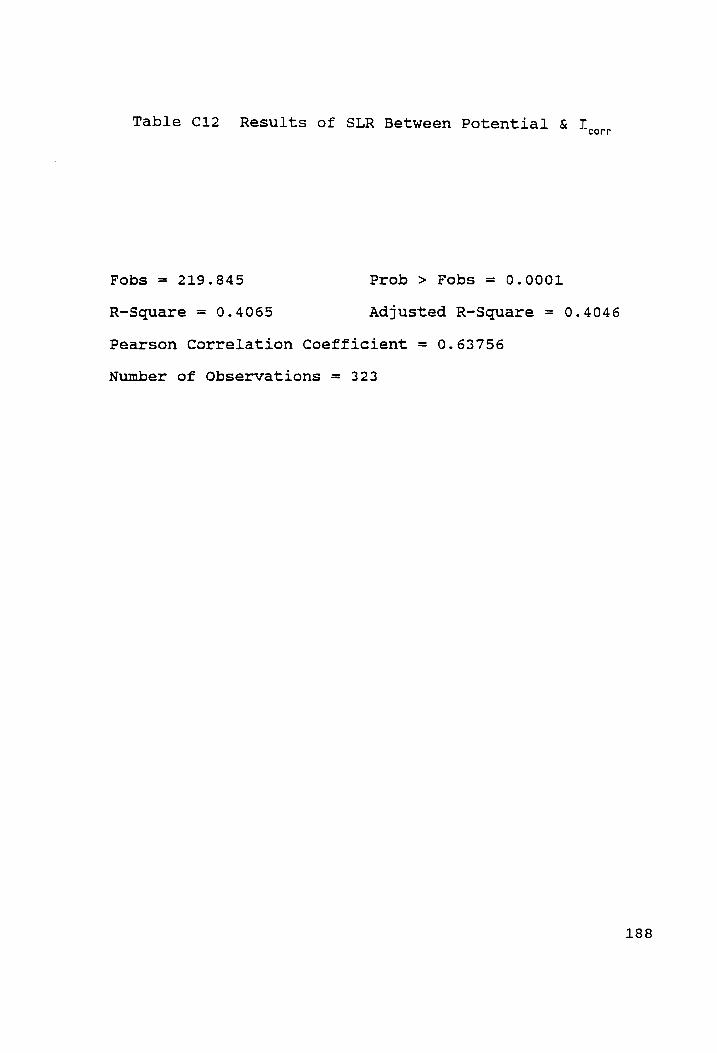
Table C12 Results of SLR Between Potential & I corr

Fobs = 219.845 Prob > Fobs = 0.0001

R-Square = 0.4065 Adjusted R~Square = 0.4046

Pearson Correlation Coefficient = 0.63756

Number of Observations = 323

188

Table C13

CLOCK

TIME

1550

1605

1620

1635

1650

1700

1720

1730

1750

1820

1840

1910

1940

2010

2040

2110

2140

2210

2240

2310

2340

0815

TIME

(min)

15

30

45

60

70

90

100

120

150

170

200

230

260

290

320

350

380

410

440

470

985

AMBIENT SURFACE

TEMP

69.1

65.8

63.3

58.7

56.6

57.0

53.2

51.4

50.1

50.5

48.5

50.9

Drying of Specimens (1",

TEMP

78.5

398.9

421.8

451.5

459.9

473.7

518.9

528.8

NA

294.8

257.7

225.0

212.9

197.6

186.2

179.0

170.0

164.0

157.1

110.4

TEMP a 1/2" BELOW TOP REBAR

PS3

76.9

97.3

136.9

165.8

187.5

207.5

213.1

211.9

203.2

194.2

183.7

175.1

167.4

160.5

153.5

148.1

142.4

98.4

PS2

74.3

94.5

126.2

150.3

169.1

188.5

195.3

193.1

185.5

178.4

170.4

162.8

156.9

150.9

144.5

140.0

134.6

93.2

PS1

77.8

105.5

153.1

190.7

212.0

239.2

248.9

247.0

238.0

230.2

221.2

211.6

203.8

196.2

188.7

183.0

176.1

120.3

230 °F)

PM3 PM2

79.9 78.1

101.2 105.7

139.3 151.1

168.5 187.5

190.9 210.4

209.8 231.9

216 243.8

212.8 241.8

202.7 233.2

194.9 226.2

185.3 217.5

175.6 208.1

167.9 200.5

161.1 193.2

154.1 185 .6

148.9 179.8

142.9 173.3

96.1 114.8

(Temp in °F)

REMARKS

Heaters turned on

height of heaters = 9"

Heaters turned off at 1825

189

AMBIENT SURFACE

Table C13

CLOCK TIME

TIME (min) TEMP

1550 0 79.5

1605 15 -

1620 30 76.7

1635 45 -

1650 60 76.3

1700 70 -

1720 90 74.5

1730 100 -

1750 120 72.6

1820 150 70.9

1840 170 69.1

1910 200 65.8

1940 230 63.3

2010 260 8658.7

2040 290 56.6

2110 320 57.0

2140 350 53.2

2210 380 51.4

2240 410 50.1

2310 440 50.5

2340 470 48.5

0815 985 50.9

TEMP

78.5

398.9

421.8

451.5

459.9

473.7

518.9

528.8

NA

294.8

257.7

225.0

212.9

197.6

186.2

179.0

170.0

164.0

157.1

110.4

TEMP 3 1/2" BELOW TOP REBAR

PM1

75.6

109.2

154.9

191.8

211.0

232.8

240.4

236.6

227.8

218.9

210.1

200.3

192.6

185 .3

177.5

171.8

164.7

110.3

(Contd. )

PC3

76.6

154.6

235.0

253.1

253.8

245.4

241.1

238.6

231.3

222.7

214.5

207.3

198.8

192.3

185.9

179.2

173.9

167.9

114.8

Drying of Specimens (1",

PC2

78.0

119.0

187.3

216.9

223.7

240.0

241.9

238.5

229.9

219.1

210.3

200.9

191.5

184.1

177.0

169.4

163.7

156.9

101.8

230 °F) (Temp in °F)

PCI

76.0

147.9

214.3

230.7

233.2

224.3

219.4

217.3

212.0

204.8

197.7

191.4

183.9

177.9

172.0

166.1

161.2

155.8

105.2

REMARKS

Heaters turned on

height of heaters = 9"

PC1 & PC3 covered with

metal sheet

PC2 covered

Heaters turned off at 1825

190

Table C14A Drying of Specimens (2",

CLOCK

TIME

1705

1715

1730

1745

1800

1810

1825

1840

1900

1915

1930

TIME

(min)

10

25

40

55

65

80

95

115

130

145

AMBIENT SURFACE TEMP @ 3" DEPTH

TEMP

60

57

57

56

56

54

53

53

52

52

50

TEMP

64.2

322.4

393.6

396.0

397.9

400.2

312.1

211.7

162.7

145.3

134.1

PM1

69.9

70.9

92.7

129.4

160.8

180.6

196.0

195.2

184.8

174.0

156.9

PM2

70.2

71.8

97.9

145.2

184.0

208.2

208.1

204.5

196.5

189.6

171.1

180

TEMP @ 2" DEPTH

PM1

69.8

82.0

136.4

189.7

220.1

229.0

219.2

207.6

190.5

185.1

169.7

PM2

61.6

84.7

148.1

210.8

229.0

233.4

222.0

211.7

197.2

188.7

168.6

°F) (Temp in °F)

REMARKS

Heaters turned on

height of heaters = 10"

PM2 covered

Heaters turned off

191

Table C14B Drying of Specimens (2", 150 °F) (Temp in °F)

CLOCK TIME AMBIENT SURFACE TEMP a 3" DEPTH REMARKS

TIME (min) TEMP TEMP PC2 PCS

1445 0 66 69.3 70.0 68.9 Heaters turned on

1500 15 67 236.5 75.5 76.8 height of heaters = 8 1/2"

1515 30 66 277.4 94.9 107.9

1530 45 66 294.6 118.2 144.8

1545 60 66 466.2 141.0 179.8 PC3 covered at 1536

Heaters turned off at 1549

1600 75 65 300.2 175.3 191.6

1605 80 65 272.1 182.0 192.1

1630 105 60 219.0 189.3 186.8

1645 129 56 197.5 186.6 180.4

1700 135 52 189.2 183.2 175.6

1715 150 50 184.1 172.5 161.7

192

Table C14C Drying of Specimens (%", 180

CLOCK

TIME

1350

1400

1410

1420

1430

1440

1450

1500

1515

1530

1545

1600

TIME

(min)

10

20

30

40

50

60

70

85

100

115

130

oF)

AMBIENT SURFACE TEMP 3 1 3/4" DEPTH TEMP @ 3/4" DEPTH

TEMP

S&B BSSSAN

ANNAN

TEMP

79.9

235.1

386.3

395.7

205.7

144.8

133.6

120.1

108.7

111.9

110.4

89.3

PM1

77.8

80.6

131.5

180.6

205.1

199.2

193.9

188.2

178.6

169.9

160.9

137.7

PM2

77.0

82.9

141.2

181.0

204.7

199.8

195.1

188.4

178.7

169.8

160.2

138.0

PM

80.8

98.6

189.5

239.5

237.3

223.4

213.8

202.4

189.3

179.3

169.1

144.0

PM2

78.9

(Temp in °F)

REMARKS

Heaters turned on

102.3 height of heaters = 10"

194.5

253.1

239.6

226.7

216.7

205.6

191.9

181.6

170.3

145.4

Heaters turned off

193

Table C14D Drying of Specimens (%",

CLOCK TIME

TIME (min)

1005 0

1015 10

1025 20

1035 30

1045 40

1055 50

1105 60

1115 70

1125 80

1135 90

1145 100

1155 110

1205 120

150 °F) (Temp in °F)

AMBIENT SURFACE TEMP 3 1 3/4" DEPTH TEMP @ 3/4" DEPTH

TEMP

52

54

54

55

56

57

58

60

61

63

TEMP

52.5

267.6

421.9

243.3

179.5

152.6

139.8

118.3

109.5

100.4

111.6

110.1

111.3

PC2

59.4

83.6

138.8

177.4

175.4

171.8

166.5

160.8

155.3

149.9

145.5

142.5

138.4

PC3

59.5

77.3

134.9

176.1

181.1

178.0

173.3

167.9

161.9

155.6

150.4

146.7

142.3

PC2

59.5

139.5

209.0

213.8

176.8

166.7

157.5

150.6

144.6

140.0

136.3

134.3

130.9

PC3

55.1

122.3

206.1

231.0

205.0

195.6

184.2

174.7

166.8

159.7

153.2

149.6

141.5

REMARKS

Heaters turned on

height of heaters = 10"

PC2 covered at 1028

Heaters turned off at 1030

194

©

Nh

a1

nO

Oo

on

—

DEPTH

OF I

MPRE

GNAT

ION

(inch)

in

.

wa q q TT q J

0 1 2 3 4 5 6 7 8 SQUARE-ROOT OF TIME (hours)

Figure Cl Depth of Impregnation vs Square-Root of Time

195

Figure C2 Non-Impregnated Sample under SEM (1 kX)

196

Figure C3 Impregnated Sample under SEM (1 kX)

197

-,.

tH ' “ i

tis pr amare heen, | -_— & = —_e -—— "

ee a am =- - - ~—- -

murSeni 2 O88okev = 3

oD

——

+ f

Figure C4 Illustrative Graph from the SEM-EDS

198

[1]

[2]

[3]

[4]

[>]

[6]

[7]

[8]

REFERENCES

Durability of Concrete Bridge Decks, Report 5, Portland

Cement Association, U.S. Bureau of Public Roads & Ten

State Highway Agencies, 46pp (1969)

Durability of Concrete Bridge Decks, Final Report,

Portland Cement Association, U.S. Bureau of Public Roads

& Ten State Highway Agencies, 35pp (1970)

Slater, J.E.,"Corrosion of Metals in Association with

Concrete", STP 818, ASTM, Philadelphia, PA, 83pp (1983)

AASHTO, FHWA, TRB, NCHRP, Strategic Highway Research

Program - Research Plans, Final Report, Technical

Research Area 43, pp TRA 4-1 thru TRA 4-60 (May 1986)

Morgan, John H., "Cathodic Protection", Leonard Hills

Books Ltd, London (1959)

Weyers, R.E. and Cady, P.D., "Development: Deep

Grooving - A Method for Impregnating Concrete Bridge

Decks", Transportation Research Record 962, pp 14-18

(1984)

Weyers, R.E. and Cady, P.D., “Application: Deep

Grooving - A Method for Impregnating Concrete Bridge

Decks", Transportation Research Record 962, pp 19-21

(1984)

Hall, Christopher, "Polymer Materials", John Wiley &

199

[9]

[10]

[11]

[12]

[13]

[14]

[15]

Sons, New York (1989)

Manson, J.A.; Chen, W.F.; Vanderhoff, J.W.; Mehta, H.C.;

Cady, P.D.; Kline, D.E. and Blankenhom, P.R., “Use of

Polymers in Highway Concrete", National Cooperative

Highway Research Program 190, TRB (1978)

Uhlig, Herbert H. and Revie, R. Winston, "Corrosion and

Corrosion Control", John Wiley & Sons (1985)

Powers, T.C., "The Nature of Concrete", Significance of

Tests and Properties of Concrete and Concrete Making

Materials, STP 169B, ASTM, pp 59-73 (1978)

Barneyback, R.S. Jr and Diamond, S., "Expression and

Analysis of Pore Fluids from Hardened Cement Pastes and

Mortars", Cement and Concrete Research, Vol 11, No. 2, pp

279-285 (1981)

Fraczek, J, "A Review of Electrochemical Principles as

Applied to Corrosion of Steel in Concrete or Grout

Environment", Corrosion, Concrete and Chlorides - Steel

Corrosion in Concrete: Causes and Restraints, SP~-102, ACI

(1987)

Cady, P.D. and Weyers, R.E., "Chloride Penetration and

Deterioration of Concrete Bridge Decks", Cement, Concrete

and Aggregates, CCAGDP, Vol 5, No. 2, pp 81-82 (Winter

1983)

Weyers, R.E., "Corrosion of Steel in Concrete", Third

International Conference, Environmental Degradation of

200

[16]

[17]

[18]

[19]

[20]

[21]

[22]

[23]

Engineering Materials, Penn State, University Park, PA,

pp 351-361 (1987)

Annual Book of ASTM Standards, C-876-87, "Standard Test

Method for Half-cell Potentials of Uncoated Reinforcing

Steel in Concrete", ASTM, Philadelphia, PA

K.C. Clear, Inc., 3LP Package - Test Procedure, Data

Analysis, Procedure and General Information (June 1988)

Test Model CL 500, Instruction Manual, James Instruments,

Inc., Chicago

Herald, S.E., "The Development of a Field Procedure for

Determining the Chloride Content of Concrete and an

Analysis in the Variability of the Effective Diffusion

Constant", M.S. Thesis in Civil Engineering, Virginia

Polytechnic Institute & State University, Blacksburg, VA

(Sept 1989)

Clear, K.C., "Reinforcing Bar Corrosion in Concrete:

Effect of Special Treatments", SP-49, ACI, Detroit,

MI, pp 71-82 (1975)

Clear, K.C., "Time to Corrosion of Reinforcing Steel in

Concrete Slab", Report # FHWA RD-76-70, FHWA, Washington,

DC (April 1976)

Nilsson Model 400 Solid State 4-Pin Soil Resistance

Meter, Instruction Manual, Nilsson Electrical Laboratory,

Inc., New York

Manning, David G., "Detecting Defects and Deterioration

201

[24]

[25]

[26]

[27]

[28]

[29]

in Highway Structures", National Cooperative Highway

Research Program, Synthesis of Highway Practice 118,

TRB, National Research Council, Washington, DC (July

1985)

Vassie, P. R., "A Survey of Site Tests for the Assessment

of Corrosion in Reinforced Concrete", LR 953, Transport

and Road Research Laboratory, England (1980)

Tremper, B., Beaton, J. L. and Stratfull, R. F., " Causes

and Repair of Deterioration to a California Bridge due to

Corrosion of Reinforcing Steel in a Marine Environment

Part II: Fundamental Factors Causing Corrosion", Highway

Research Bulletin 182, TRB, National Research Council, pp

18-41, Washington, DC (1958)

Browne, R. D., “Mechanisms of Corrosion of Steel in

Concrete in Relation to Design, Inspection and Repair of

Offshore and Coastal Structures", Performance of Concrete

in a Marine Environment, SP-65, ACI, pp 169-204

(1980)

Micromeritics Autopore 9200, Mercury Porosimeter,

Instruction Manual

Hearle, J. W. S., Sparrow, J. T. and Cross, P. M., " The

Use of the Scanning Electron Microscope", Pergamon Press

(1972)

Gabriel, Barbra L., "SEM: A User's Manual for Materials

Science", ASM, Metals Park, OH (1985)

202

VITA

Tapas Dutta was born in Calcutta, India on May 21, 1963. He

completed his Bachelor of Civil Engineering at Jadavpur

University, Calcutta, India in 1988. He started his graduate

studies at Virginia Polytechnic Institute & State University

in January 1989 on Transportation Materials in the Civil

Engineering Department.

4 apabyde”

203