APPROVED: Cue Kh Soler - VTechWorks

LOAD TRANSFER IN THE STIFFENER-TO-SKIN JOINTS

OF A PRESSURIZED FUSELAGE

by

Naveen Rastogi

Dissertation submitted to the Faculty of the

Virginia Polytechnic Institute and State University

in partial fulfillment of the requirements for the degree of

DOCTOR OF PHILOSOPHY

in

Aerospace Engineering

APPROVED: Cue Kh Soler

Dr. Eric R. Jolthson. Chairman

Hla

Dr. Rakesh

. W. Hyer . Kapania

Dr. OAL Grifan, — “Dr. E. Nikolaidis

4 SG

Dr. Z. Girdal

February, 1995

Blacksburg, Virginia

LOAD TRANSFER IN THE STIFFENER-TO-SKIN JOINTS

OF A PRESSURIZED FUSELAGE

by

Naveen Rastogi

Committee Chairman: Dr. Eric R. Johnson

Aerospace Engineering

(ABSTRACT)

Structural analyses are developed to determine the linear elastic and the geo-

metrically nonlinear elastic response of an internally pressurized, orthogonally stiff-

ened, composite material cylindrical shell. The configuration is a long circular cylin-

drical shell stiffened on the inside by a regular arrangement of identical stringers

and identical rings. Periodicity permits the analysis of a unit cell model consisting

of a portion of the shell wall centered over one stringer-ring joint. The stringer-

ring-shell joint is modeled in an idealized manner; the stiffeners are mathematically

permitted to pass through one another without contact, but do interact indirectly

through their mutual contact with the shell at the joint. Discrete beams models of

the stiffeners include a stringer with a symmetrical cross section and a ring with

either a symmetrical or an asymmetrical open section. Mathematical formulations

presented for the linear response include the effect of transverse shear deformations

and the effect of warping of the ring’s cross section due to torsion. These effects

are important when the ring has an asymmetrical cross section because the loss of

symmetry in the problem results in torsion and out-of-plane bending of the ring,

and a concomitant rotation of the joint at the stiffener intersection about the cir-

cumferential axis. Data from a composite material crown panel typical of a large

transport fuselage structure are used for two numerical examples. Although the

inclusion of geometric nonlinearity reduces the “pillowing” of the shell, it 1s found

that bending is localized to a narrow region near the stiffener. Including warping

deformation of the ring into the analysis changes the sense of the joint rotation.

Transverse shear deformation models result in increased joint flexibility.

ACKNOWLEDGEMENTS

I would like to express sincere gratitude to my advisor Prof. Eric R. Johnson

for his contribution to my academic and professional development. His invaluable

guidance at every step of this work has been a constant source of encouragement

for me. I am grateful to my other committee members, Profs. E. Nikolaidis, M.

W. Hyer, O. H. Griffin, Jr., R. K. Kapania, and Z. Gurdal for serving on my

committee and reading my dissertation. Finally, I would like to thank my wife Ritu

and daughter Apoorva for their understanding and moral support through out the

course of this work.

This work is supported by the Structural Mechanics Branch, NASA Langley

Research Center, under the grant NAG-1-537. The support is gratefully acknowl-

edged.

iv

TABLE OF CONTENTS

Abstract

Acknowledgements

List of Tables

List of Figures

1. Introduction

1.1 Composite Materials in Primary Structures

1.2 Fuselage Loads and Design

1.3 Stiffener-to-Skin Joints .

1.4 Contact Problems

1.5 Pressurized, Stiffened Shells

1.6 Objectives

1.7 Problem Definition

1.8 Analysis Approach

2. Governing Equations for Linear Analyses

2.1 Structural Model and Assumptions

2.2 Transverse Shear Deformation Formulations

2.2.1 Shell

2.2.1.1 Strain-Displacement Relations

2.2.1.2 Virtual Work

2.2.1.3 Constitutive Relations

2.2.1.4 Equilibrium Equations

2.2.1.5 Boundary Conditions

2.2.2 Stringer

il

iv

xi

QO bd

~]

. 10

. 14

2.2.3 Ring

2.3 Classical Formulations

2.3.1 Shell

2.3.1.1 Strain-Displacement Relations

2.3.1.2 Virtual Work

2.3.1.3 Constitutive Relations

2.3.2 Stringer

2.3.3 Ring

2.4 Displacement Continuity

2.5 Augmented Virtual Work for the Assembly

3. Governing Equations for Nonlinear Analysis

3.1 Analytical Model and Assumptions

3.2 Shell

3.2.1 Strain-Displacement Relations .

3.2.2 Internal Virtual Work

3.2.3 External Virtual Work

3.3 Stringer

3.4 Ring

3.5 Incremental Virtual Work

3.5.1 Shell

3.5.2 Stringer

3.5.3 Ring

3.6 Displacement Continuity

3.7 Augmented Virtual Work Terms

4. Fourier Approximations and Solution Procedure

4.1 Introduction

. dl

. 30

. 30

. 36

. 36

. 37

. 38

. 38

44

. 44

. 45

. 45

. 46

. 46

. o9

. 09

. 60

. 62

. 63

. 64

. 64

. 65

67

. 67

vi

4.2 Displacements and Rotations Approximations ......... . 68

421Shel 2... ee, J. . . 68

4.2.2 Stringer . . . 69

42.3 Ring . 2... . ee ee ee ee ee 70

4.3 Interacting Load Approximations . . Lo .... 71

4.3.1 Shell-Stringer . 2... 2... .. Tl

4.3.2 Shell-Ring 2... 2... 2. ee 72

4.4 Terms Omitted in the Fourier Series . . . . 2. . . 18

4.4.1 Rigid Body Equilibrium for Ring . . . . 13

4.4.2 Rigid Body Equilibrium for Stringer . .......2. =.=. =. 78

4.4.3 Terms Omitted 2... .....2.2, . . 18

4.5 Discrete Equations and their Solution . . . 80

4.5.1 Linear Analyses . 2... 2... ee ee ee ee. 80

4.5.1.1 Transverse Shear Deformation Model . . . . &l

4.5.1.2 Classical Model . 2... 2. 2... 82

4.5.2 Nonlinear Analysis ......... 15)

4.5.3 Verification of Numerical Solution ..... . . . 89

5. A Unit Cell Model with Symmetric Stiffeners 90

5.1 Introduction... 2... ee ee ee ee. 90

5.2 Numerical Data . ....... ; ; . . 90

5.3 Validation of Structural Model . ......... 2... 91

5.4 Linear Response Versus Nonlinear Response. : , . . 96

5.4.1 Pillowing ...........2.22. , , . . 96

5.4.2 Bending Boundary Layer .......... , . . 99

5.4.3 Interacting Load Distributions . , , , . 104

5.4.4 Stiffener Actions ....... , , . . 109

Vil

5.5 Singularity at the Shell-Stringer-Ring Joint

5.6 Summary of Results

6. A Unit Cell Model with an Asymmetric Ring

6.1 Introduction

6.2 Numerical Data

6.3 Influence of an Asymmetrical Section Ring

6.3.1 Interacting Load Distributions

6.3.2 Resultants at the Stiffener Intersection

6.3.2.1 Comparison of Pull-Off Load

6.3.3 Singular Behavior at the Joint

6.3.4 Stiffener Actions

6.3.5 Shell Response

6.4 A Ring with Symmetrical Cross Section

6.5 Summary of Results

7. Concluding Remarks

7.1 Summary

7.2 Concluding Remarks

7.2.1 Effect of Geometric Nonlinearity .

7.2.2 Influence of an Asymmetrical Section Ring

7.2.3 Singularity at the Shell-Stringer-Ring Joint

7.38 Recommendations for Future Work

References

Nomenclature

Appendix A

Elements of matrices for linear analysis using transverse shear

deformation model

154

155

157

158

159

163

166

vill

Appendix B

Elements of matrices for linear analysis using classical model

Appendix C

Elements of tangent stiffness and load stiffness matrices for nonlinear

analysis

Appendix D

Elements of residual force vectors for nonlinear analysis

VITA

172

178

198

209

1X

LIST OF TABLES

6.1 Effect of transverse shear and warping on the interacting line load intensities

and their distributions along the contact limes .......2.... 121

6.2 Rotations about the circumferential axis at the stiffener intersection . . 132

6.3 Resultants at the stiffener intersection .............. . 136

1.1

1.2

1.3

2.1

2.2

2.3

3.1

3.2

3.3

3.4

4.1

4.2

5.1

5.2

5.3

5.4

LIST OF FIGURES

Orthogonally stiffened cylindrical shell subjected to internal pressure

Repeating unit of an orthogonally stiffened cylindrical shell

Interacting line load intensities shown in the positive sense acting on the

inside surface of the shell

Displacements and rotations for shell

Displacements and rotations for stringer .

Displacements and rotations for ring

Enclosed volume of a repeating unit .

Position vector and elemental area of the deformed upper surface

Image of diameter POQ in the deformed state is P'O'Q’ with O' on the

axis of revolution

Stiffened shell of (a) three, and (b) four unit cells

Cylindrical coordinates (x,¢, Rg + €) of a typical point P in the ring .

Structure of shell stiffness matrix [Ay] for classical structural model, linear analysis, and for generic values of m and n

Circumferential distribution of the shell’s normal displacement from

the linear analysis at 10 psi

Axial distribution of the shell’s normal displacement from the linear

analysis at 10 psi

Circumferential normal strain on the inner and outer shell surfaces from

the linear analysis at 10 psi

Axial normal strain on the inner and outer shell surfaces from the hnear

analysis at 10 psi

_ Ii

18

. 18

. 29

. 32

AT

. 49

. OO

. 14

. 84

. 92

. 93

. 94

. 95

xi

3.0

5.6

5.7

5.8

5.9

5.10

5.11

5.12

9.13

5.14

9.15

5.16

5.17

5.18

6.1

Circumferential distribution of the shell’s normal displacement from

the nonlinear analysis at 10 psi

Axial distribution of the shell’s normal displacement from the nonlinear

analysis at 10 psi

Circumferential normal strain on the inner and outer shell surfaces from

the nonlinear analysis at 10 psi

Axial normal strain on the inner and outer shell surfaces from the

nonlinear analysis at 10 psi .

Distribution of the shell’s circumferential bending moment midway between the rings (zr = —l) at 10 psi .

Distribution of the shell’s circumferential transverse shear resultant

midway between the rings (x = —/) at 10 psi

Tangential component of the line load acting on the shell due to the

ring at 10 psi .

Normal component of the line load acting on the shell due to the

ring at 10 psi .

Tangential component of the line load acting on the shell due to the stringer at 10 psi

Normal component of the line load acting on the shell due to the

stringer at 10 psi

Stringer axial force and bending moment distributions at 10 psi .

Ring circumferential force and bending moment distributions at 10 psi .

Normal load intensity A, and total normal load F, at the stiffener

intersection for increasing number of harmonics in the linear analysis

at 10 psi .

Normal load intensity A, and total normal load F, at the stiffener

intersection for increasing number of harmonics in nonlinear analysis

at 10 psi .

Stiffener cross sections

. 98

100

101

102

103

105

106

107

108

110

111

113

114

119

xX

6.2

6.3

6.4

6.5

6.6

6.7

6.8

6.9

6.10

6.11

6.12

6.13

6.14

6.15

6.16

6.17

6.18

6.19

6.20

Stringer-shell tangential force intensity in axial direction at 10 psi .

Stringer-shell normal force intensity at 10 psi .

Ring-shell axial force intensity in circumferential direction at 10 psi

Ring-shell tangential force intensity in circumferential direction

at 10 psi .

Ring-shell normal force intensity at 10 psi

Ring-shell tangential moment intensity in circumferetial direction

at 10 psi .

Ring-shell normal moment intensity at 10 psi .

Joint rotations for (a) the classical structural models, and (b) for transverse shear deformable models

Components of the resultant of the interacting line load intensities acting on the inside wall of the shell at the origin

Stringer axial force and bending moment distribution at 10 psi

Stringer transverse shear force distribution at 10 psi .

Ring circumferential force and in-plane bending moment distributions

at 10 psi .

Ring in-plane shear force distribution at 10 psi

Ring out-of-plane bending moment and torque distributions at 10 psi

Ring out-of-plane shear force distribution at 10 psi

Distribution of shell’s normal displacement at 10 psi .

Distributions of the axial normal strain on the inner and outer shell

surfaces midway between the stringers (6 = —O) at 10 psi

Distributions of the circumferential normal strain on the inner and outer

shell surfaces midway between the rings (rx = —!) at 10 psi

Ring-shell tangential force intensity in circumferential direction for a ring with symmetrical cross section at 10 psi

122

123

124

128

129

131

134

138

139

148

149

Xi

CHAPTER 1

INTRODUCTION

1.1 COMPOSITE MATERIALS IN PRIMARY STRUCTURES

Composite materials are being used increasingly for variety of structural applica-

tions in aerospace engineering and other related weight sensitive applications where high

strength-to-weight and stiffness-to-weight ratios are required. The success of composite

materials results from the ability to make use of the outstanding strength, stiffness and

low specific gravity of fibres such as glass, graphite or Kevlar. When superior specific

mechanical properties are combined with the unique flexibility in design and the ease of

fabrication that composites offer, it is no wonder that their growth rate has far surpassed

that of other materials.

Development of the state-of-the-art manufacturing techniques has made it possible

to replace complicated structural components/assemblies by single co-cured or adhesively

bonded composite parts, thereby minimizing the number of fasteners to be used in a

structure, and hence, enhancing the structural integrity. While the use of bonded com-

posite structures as secondary and tertiary load carrying members has been widespread

in aerospace industry, their use as primary load carrying members is still very limited.

Most of the applications of composites as primary structural components have been in the

area of fabrication of empennage or control surfaces of an aircraft. Thus, the potential of

composite materials as a primary load carrying structure, such as fuselage of an aircraft,

has not been fully realized yet. One of the main reasons for this could be the lack of

confidence of aerospace industry in utilizing composite materials for fuselage manufactur-

ing, which, in turn, could be due to the lack of a full scale analysis, design, and testing

1

to qualify composite materials for use in the fuselage of both civil and military transport

aircraft.

1.2 FUSELAGE LOADS AND DESIGN

As described in the text by Niut, the loads affecting fuselage design of a transport

aircraft can result from flight maneuvers, landings, cabin pressurization and ground han-

dling, etc. Fuselage (or cabin) pressurization of a transport aircraft induces hoop and

longitudinal stresses in the fuselage. The fuselage internal pressure depends on the cruise

altitude and the comfort desired for the flight crew and/or passengers, and can cause a

pressure differential of up to 10 psi across the fuselage skin. An unstiffened, or monocoque,

fuselage would carry this internal pressure load as a shell in membrane response, like a

pressure vessel. However, internal longitudinal and transverse stiffeners are necessary to

carry the loads resulting from flight maneuvers, landings, and ground handling, etc. The

longitudinal stiffeners, called stringers or longerons, carry the major portion of the fuse-

lage bending moment. The transverse stiffeners, called frames or rings, are spaced at

regular intervals along the length of the fuselage to prevent buckling of the longitudinals

and maintain cross-sectional shape of the fuselage. The presence of these internal stiffen-

ers introduces the following two important aspects in the fuselage design of a transport

aircraft:

1. The stiffeners, i.e. stringers and rings, are attached to the fuselage skin by some

kind of fasteners, or perhaps bonded to it. Thus, there is a transmission of loads between

the skin and the stiffeners all along their attachment lines, and at the stiffeners’ intersection

a local concentration of the interacting loads due to joint stiffness occurs. Understanding of

the load transfer mechanism in the stiffener-to-skin joints under pressurization is necessary

for determining the load capacity of these joints.

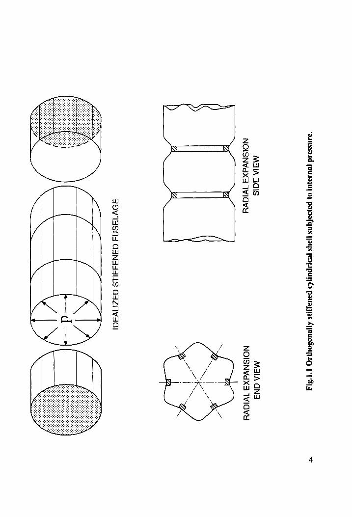
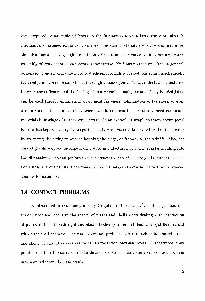
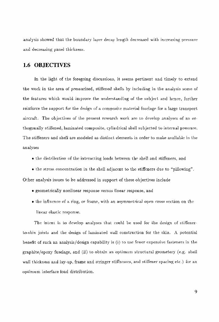
2. The presence of internal stiffeners, particularly the presence of frames or rings,

prevents expansion of the fuselage skin as a membrane, and the skin bulges, or “pillows”,

between the stiffeners under the action of the internal presure as shown in Fig. 1.1. Hence,

where the skin is restrained against its expansion as a membrane along the stiffeners, a

bending boundary layer is formed.

1.3 STIFFENER-TO-SKIN JOINTS

The design of stiffener-to-skin joints was cited by Jackson et al.” as one of the major

technology issues in utilizing graphite/epoxy composites in the fuselage of a large transport

aircraft. In order to realize the full potential of advanced composites in lightweight aircraft

structure, it is particularly important to ensure that the joints, either adhesively bonded

or mechanically fastened, do not impose a reduced efficiency on the structure and should

be cost effective as well. The use of graphite/epoxy composites in conjunction with metal

fasteners in conventional, mechanically fastened joints is a critical design factor. Improper

coupling of joint materials can cause serious corrosion problems to metals because of the

difference in electric potential between these metals and graphite. In other words, insuring

the galvanic compatibility of fastener materials with graphite composites is essential to

avoid corrosion problems in the structure?*.

It has been established that materials such as titanium, corrosion-resistant steels,

nickel and cobalt alloys can be coupled to graphite composites without such corrosive

effects. In contrast, aluminum, magnesium and stainless steel are most adversely affected

because of the difference in electric potential between these materials and graphite, and

their use would lead to serious corrosion problems in the structure. However, fasteners

made of materials such as titanium, corrosion-resistant steels, nickel and cobalt alloys

are much more expensive than the more conventional fastner materials like aluminum,

magnesium and stainless steel, etc. With thousands of fasteners, e.g., rivets, bolts, nuts,

3

‘aunssaid jBusajUy

0} pazydafqns

jays pBdyapuyAD

pauayys AjpeuosouIO [13h

MalA SdIs

MalA CNS

NOISNVdXa4 1VI0VY

NOISNVdXa4 WIOQVd

% Yi

NY

A9DV1ASNA QANAsSAILS

GAZINVAAI

Lo

Lo Lf

£

|

[ ff

YX

NNN.

NON

d

etc. required to assemble stiffeners to the fuselage skin for a large transport aircraft,

mechanically fastened joints using corrosion-resistant materials are costly and may offset

the advantages of using high strength-to-weight composite materials in structures where

assembly of two or more components is imperative. Niu! has pointed out that, in general,

adhesively bonded joints are more cost efficient for lightly loaded joints, and mechanically

fastened joints are more cost efficient for highly loaded joints. Thus, if the loads transferred

between the stiffeners and the fuselage skin are small enough, the adhesively bonded joints

can be used thereby eliminating all or most fasteners. Elimination of fasteners, or even

a reduction in the number of fasteners, would enhance the use of advanced composite

materials in fuselage of a transport aircraft. As an example, a graphite-epoxy crown panel

for the fuselage of a large transport aircraft was recently fabricated without fasteners

by co-curing the stringers and co-bonding the rings, or frames, to the skin’®. Also, the

curved graphite-epoxy fuselage frames were manufactured by resin transfer molding into

two-dimensional braided preforms of net structural shape’. Clearly, the strength of the

bond line is a critical issue for these primary fuselage structures made from advanced

composite materials.

1.4 CONTACT PROBLEMS

As described in the monograph by Grigoluk and Tolkachev®, contact (or load dif-

fusion) problems occur in the theory of plates and shells when dealing with interaction

of plates and shells with rigid and elastic bodies (stamps), stiffening ribs/stiffeners, and

with plate-shell contacts. The class of contact problems can also include laminated plates

and shells, if one introduces reactions of interaction between layers. Furthermore, they

pointed out that the selection of the theory used to formulate the given contact problem

may also influence the final results.

The study of load diffusion in the stiffener-to-skin joints of an orthogonally stiffened

shell subjected to internal pressure is also a shell contact problem. The type of structural

theory used to model the discrete elements, i.e., the shell, the stringer, and the ring,

influences the distribution of the interacting loads at the shell-stiffener interface. A brief

literature survey on the work done in the area of contact problems is presented in the

remainder of this section.

Contact problems have always attracted scientists, academicians and designers alike

because of their inherent importance for any structure analysis involving an assembly of

two or more components. The first work is by Melan?, who considered a semi-infinite

plate with an infinite stiffener attached to its edge. A concentrated longitudinal force is

applied to the stiffener. In 1932, Melan obtained a closed form solution for tangential

forces in the plate along the line of stiffener attachment and also for the axial force in the

}!°, in 1948, analyzed a semi-infinite plate to which a semi-infinite stiffener stiffener. Buel

is attached, loaded at the origin with a longitudinal force. An infinite series solution for

the airy stress function reduced the problem to an infinite set of algebraic equations, and

Buell obtained a numerical solution by reducing the set to six equations in six unknowns.

A solution to Buell’s problem and an identical problem for an infinite plate were obtained

by Koiter! in 1955. Using as a Green’s function the solution with a concentrated force,

Koiter obtained a singular integral equation for the interacting tangential force between

the stiffener and the plate. Through a series of complex mathematical steps using Mellin

transformation, Koiter found the longitudinal force in the stiffener as an infinite series.

Koiter’s solution can serve as a criterion of exactness of Buell’s numerical solution.

The load diffusion problem for a finite stiffener attached to an infinite plate was first

solved by Benscooter!? in 1949. He obtained an integro-differential equation, of the same

form as the Prandtl equation for the distribution of aerodynamic forces in aircraft wing

6

(also known as monoplane equation), with stiffener axial force as an unknown variable.

First, Benscooter expanded the variable into a series of Chebyshev polynomials of the

second kind to obtain the discretized equations, and then solved them for unknown coef-

ficients. Budiansky and Wu! extended Melan’s problem for the case where the stiffener

is rivetted to the plate at discrete points with constant spacing. Subsequent to some of

these landmark works, numerous authors have studied the load diffusion problem between

sheet and stiffener. An extensive biblography on the subject is given in Chapter 3 of Ref.

[8].

As for circular cylindrical shells stiffened by longtudinal stiffeners, studies are few.

Fischer!4 was the first to analyze an infinitely long circular cylindrical shell reinforced by

equally spaced, continuously attached longitudinal stiffeners, each stiffener being loaded by

a single concentrated longitudinal force (a counterpart of Melan’s plate problem). Fischer

accounted for bending of stiffeners and obtained a solution for the membrane shearing

stress transmitted by a loaded stringer to the shell, and the axial stress developed within

the stringer. Grigoluk and Tolkachev® also analyzed this problem but did not take into

account the bending of stiffeners. A detailed biblography on some other types of shell

contact problems can be found in Chapter 8 of Ref. [8].

1.5 PRESSURIZED, STIFFENED SHELLS

A literature survey on the work done in the area of stiffened shells under internal

pressure suggests that in the past, only a few studies have been carried out in this area. In

1952, Flugge!® studied the stress problems in pressurized cabins of high altitude aircraft

by dividing it into two problems. First problem was concerned with curved walls of the

cabin or pressure vessel, hence was called shell problem. The second problem, called the

plate problem, was concerned with small rectangular panels of the cabin wall, framed

by stiffeners. Of interest here are the former problems where Fligge obtained analytical

7

expressions for stresses in the shell and the stiffeners (i.e., stringer and ring) for a single

cylinder model, and a double cylinder model, using a smeared stiffness approach. In 1958,

Houghton’® computed the stresses occuring in stringer reinforced pressurized cylindrical

shells due to restraining action of the frames. He presented results showing the effect of

variation of frame pitch and stiffness on the bending moment and shear force in the skins,

and the hoop stress in the skins between the frames. Houghton’s analysis was limited

to metallic components, and did not take into account the eccentricity of stiffeners with

respect to the skin. Pressure-cabin problems are described in Chapter 9 of Williams!”

1960 text on aircraft structures. In the preface Williams justified the need for a chapter

devoted to this subject on the importance of high speed civil air-transport. The effect of

frames and bulkheads on the stresses in a cabin shell was considered in some detail, and

it was shown how the presence of reinforcing stringers de-localizes the constricting effect

of a frame or bulkhead. Williams analyses were also limited to metallic components, and

did not take into account the eccentricity of stiffeners with respect to the skin. Wang!®, in

1970, carried out a discrete analysis of a metallic, orthogonally stiffened cylindrical shell

subjected to internal pressure. Stiffener eccentricity, the normal component of interacting

load between shell and stiffeners, and closed-end pressure vessel effects were taken into

account. In 1985, Wang and Hsu‘? improved the earlier work by including in the analysis,

a composite material shell wall, interacting shear forces between the skin and stiffeners,

and a direct accounting of closed-end pressure vessel effects. In both of these works, the

results were obtained for a linear elastic response and symmetric stiffeners. Skin-stiffener

interactions were computed but results for them were not presented. In 1985, Boitnott?°

examined by experiment and analysis the pressure pillowing of a cylindrical composite

panel clamped in a stiff fixture. Boitnott’s geometrically nonlinear analysis correlated

well with the experiments when panel slip from the fixture was taken into account. The

8

analysis showed that the boundary layer decay length decreased with increasing pressure

and decreasing panel thickness.

1.6 OBJECTIVES

In the light of the foregoing discussions, it seems pertinent and timely to extend

the work in the area of pressurized, stiffened shells by including in the analysis some of

the features which would improve the understanding of the subject and hence, further

reinforce the support for the design of a composite material fuselage for a large transport

aircraft. The objectives of the present research work are to develop analyses of an or-

thogonally stiffened, laminated composite, cylindrical shell subjected to internal pressure.

The stiffeners and shell are modeled as distinct elements in order to make available in the

analyses

e the distribution of the interacting loads between the shell and stiffeners, and

e the stress concentration in the shell adjacent to the stiffeners due to “pillowing”.

Other analysis issues to be addressed in support of these objectives include

e geometrically nonlinear response versus linear response, and

e the influence of a ring, or frame, with an asymmetrical open cross section on the

linear elastic response.

The intent is to develop analyses that could be used for the design of stiffener-

to-skin joints and the design of laminated wall construction for the skin. A potential

benefit of such an analysis/design capability is (i) to use fewer expensive fasteners in the

graphite/epoxy fuselage, and (ii) to obtain an optimum structural geometery (e.g. shell

wall thickness and lay-up, frame and stringer stiffnesses, and stiffener spacing etc.) for an

optimum interface load distribution.

1.7 PROBLEM DEFINITION

An idealized model is assumed for the semi-monocoque fuselage. This configuration

is a closed-end, stiffened, pressurized shell in which closure is mathematically presumed to

occur at infinity. The long circular cylindrical shell is stiffened on the inside by a regular

arrangement of identical stringers and identical rings (frames). With respect to the applied

internal pressure load, which is assumed spatially uniform, the model is periodic in the

circumferential and longitudinal directions both in geometry and in material properties.

Periodicity of this configuration permits the analysis of a portion of the shell wall centered

over a generic stringer-ring joint as shown in Fig. 1.2; i.e., deformation of a structural

unit cell (or repeating unit) determines the deformation of the entire stiffened shell. The

radius of the middle surface of the undeformed cylindrical shell is denoted by R, and the

thickness of the shell is denoted by ¢. Axial coordinate z and the circumferential angle @

are lines of curvature on the middle surface, and the thickness coordinate is denoted by z,

with —t/2 < z<t/2. The origin of the surface coordinates is centered over the stiffeners’

intersection so that -l << 4 <land -O < @< Q, where 2/ is the axial length, and 2RO

is the circumferential arc length of the repeating unit. The stringer is assumed to have

a symmetrical cross section, and the frame is assumed to have either an asymmetrical

or a symmetrical open section. Asymmetrical open section frames are commonly used

as transverse stiffeners in the fuselage structure. The stiffeners are modeled as discrete

beams perfectly bonded to the inside shell wall, so that the interacting loads between

the stiffeners and shell wall are line load intensities. These line load intensities represent

resultants of the tractions integrated across the width of the attachment flanges of the

stiffeners.

Mathematical formulations for the linear elastic and a geometrically nonlinear elastic

response are presented in this work. The formulations for the linear elastic response

10

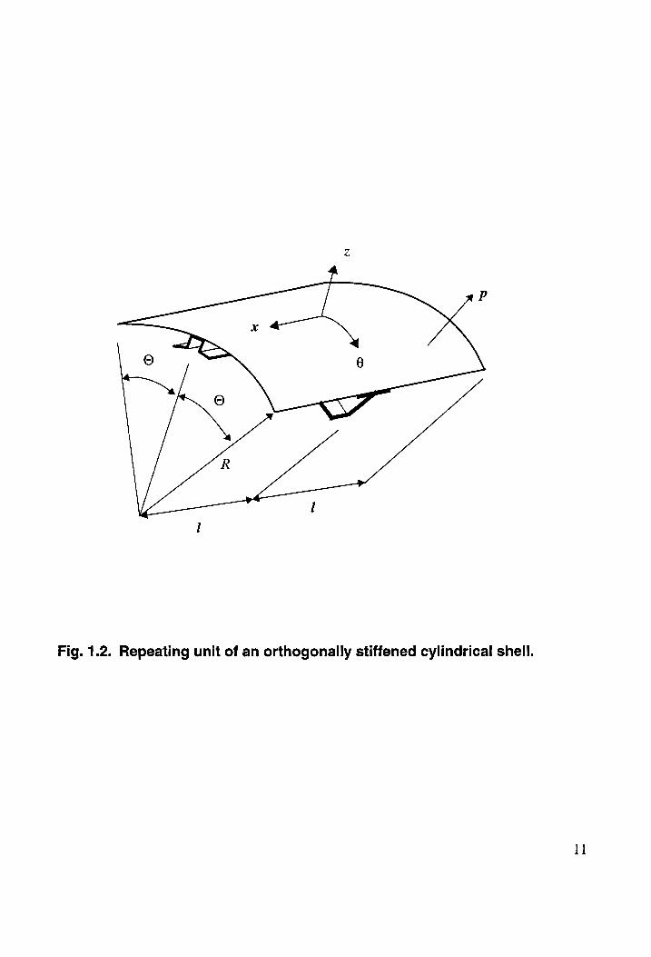
Fig. 1.2. Repeating unit of an orthogonally stiffened cylindrical shell.

11

include the effect of transverse shear deformations and the effect of warping deformation

of the ring’s cross section due to torsion. These effects are important when the ring has

an asymmetrical cross section, because the loss of symmetry in the problem results in

torsion of the ring, as well as out-of-plane bending, and a concomitant rotation of the

joint at the stiffener intersection about the circumferential axis. For symmetric section

stiffeners, the response of the unit cell (see Fig. 1.2) is symmetric about the stringer axis

and the ring axis, and there is no rotation of stringer-ring-shell joint. The formulations

for a geometrically nonlinear response are presented for symmetric stiffeners only, and are

based on classical theory. The stringer-ring-shell joint is modeled in an idealized manner;

the stiffeners are mathematically permitted to pass through one another without contact,

but do interact indirectly through their mutual contact with the shell at the joint.

On the basis of the symmetry about the z-axis for the unit, only the interacting line

load components tangent and normal to the stringer are included in the analysis. However,

due to the ring’s asymmetrical cross section, the components of line loads between shell

and the ring consist of three force intensities and two moment intensities. The shell-

stringer interacting force components per unit length along the contact lines are denoted

by Azs(x) for the component tangent to the stringer, and A_,(x) for the component normal

to the stringer. The three shell-ring interacting force components per unit length along

the contact lines are denoted by A,,(@) for the component acting in the axial direction,

Aer(@) for the component tangent to the ring, and A,,(@) for the component normal to

the ring. The two shell-ring interacting moment components per unit length along the

contact lines are denoted by Ag,(@) for the component tangent to the ring, and A-,(@) for

the component normal to the ring. These interacting loads acting in a positive sense on

the inside surface of the shell are shown in Fig. 1.3.

12

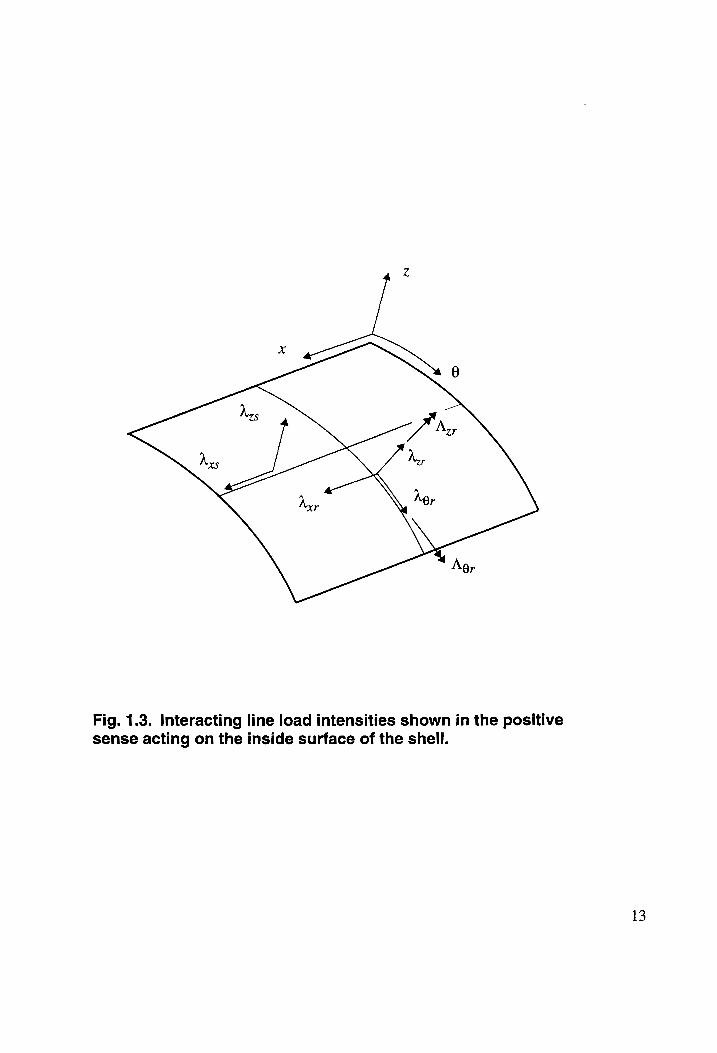
Fig. 1.3. Interacting line load intensities shown in the positive

sense acting on the inside surface of the shell.

13

1.8 ANALYSIS APPROACH

For both the linear elastic and geometrically nonlinear elastic response of the repeat-

ing unit to internal pressure, the Ritz method is used. The principle of virtual work is

applied separately to the shell, stringer and ring. Displacements are individually assumed

for the shell, stringer, and the ring as Fourier Series expansions. The virtual work func-

tionals are augmented by Lagrange multipliers to enforce kinematic constraints between

the structural components of the repeating unit. As a result, point-wise displacement con-

tinuity between structural elements is achieved. The Lagrange multipliers represent the

interacting line loads between the stiffeners and the shell, and are also expanded in Fourier

Series. Closed-end pressure vessel effects are included. Data for the example problems are

representative of the dimensions of large transport fuselage structure.

The primary advantage of using the analysis approach discussed above results from

the fact that a point-wise displacement continuity is achieved between the structural

elements. In commercial finite element analysis codes viz., ABAQUS?!, NASTRAN??,

etc., the interpolation functions used for the displacement fields of the structural elements

(e.g., the shell and beam elements) are, in general, not the same. Thus, the continuity

between the structural elements can only be satisfied at discrete points, i.e., at the nodes.

Another shortcoming of these finite element codes is that they can not model the torsional

warping deformation of an open section, laminated, curved beam. This is a disadvantage

since the restraint of warping deformation in the ring due to continous contact with

the shell results in significant circumferential normal stresses in the ring. To account

for torsional warping deformation in the ring, the ring would have to be modeled as a

branched shell with these finite element codes. Branched shell models of the stiffeners

would significantly increase the degrees-of-freedom in the finite element model. It should

be mentioned that beam models including torsional warping deformation require seven

14

nodal degrees of freedom between elements. The seventh degree of freedom is related to

the rate of twist. However, it is standard in finite element codes to have only six nodal

degrees of freedom (three displacements and three rotations) between one-dimensional

elements.

15

CHAPTER 2

GOVERNING EQUATIONS FOR LINEAR ANALYSES

2.1 STRUCTURAL MODEL AND ASSUMPTIONS

Linear elastic analyses are carried out for a unit cell model (Fig. 1.2) defined in

Section 1.7 of an internally pressurized, orthogonally stiffened, long circular cylindrical

shell. The interacting line loads between the shell and stiffeners acting in a positive

sense on the inside surface of the shell are shown in Fig. 1.3. For a symmetrical section

ring, the repeating unit (or unit cell model) is symmetric about 6-axis as well, which

implies that there is no out-of-plane bending and torsion of the ring, and consequently, no

rotation of the joint at the stiffener intersection about the circumferential axis. Thus, for

the symmetrical section stiffeners only the interacting line load components tangent and

normal to the stiffeners are non-zero.

Mathematical formulations for the linear elastic response presented in this chapter

include the effect of transverse shear deformations and the effect of warping deformation

of the ring’s cross section due to torsion. These effects are important when the ring has

an asymmetrical cross section, because the loss of symmetry in the problem results in

torsion of the ring, as well as out-of-plane bending, and a concomitant rotation of the

joint at the stiffener intersection about the circumferential axis. This stringer-ring-shell

joint is modeled in an idealized manner; the stiffeners are mathematically permitted to

pass through one another without contact, but do interact indirectly through their mutual

contact with the shell at the joint. Restraint of cross-sectional warping, as occurs here in

the ring due to contact with the shell, is an important contributor to the normal stresses in

thin-walled open section bars, as was demonstrated by Hoff??. Based on transverse shear

deformation and cross-sectional warping of the ring, four structural models are defined.

16

The simplest model uses non-transverse-shear-deformable theory, or classical theory, and

neglects warping due to torsion. The most complex model includes both effects. Models

of intermediate complexity occur for inclusion of one effect without the other.

The purpose of linear elastic analyses is two fold. First, the linear elastic analy-

sis developed in this chapter is compared with a geometrically nonlinear elastic analysis

developed in Chapter 3 for the unit cell model with symmetrical cross section stiffeners.

Second, the effect of skin-stringer-ring joint flexibility, and the effect of warping of the

ting’s cross section due to torsion, on the response are quantified. The following gen-

eral assumptions, which are valid for classical as well as transverse shear deformation

formulations, are made for linear elastic analyses of the unit cell model:

1. Normals to the undeformed reference surface remain straight and are

inextensional.

2. Material behavior is linearly elastic.

3. The thickness normal stress is assumed to be small with respect to the normal

stresses in the axial and circumferential directions, and hence it is neglected

in the material law.

2.2 TRANSVERSE SHEAR DEFORMATION FORMULATIONS

2.2.1 SHELL

A consistent first order transverse shear deformation theory is developed to model

the shell. Based on the assumption that the shell thickness tis relatively small and hence,

does not change during loading, the displacements at an arbitrary material point in the

shell are approximated by

U(z,0,7z) = u(z,@) + z¢,(2,8) (2.1)

17

b,

ar

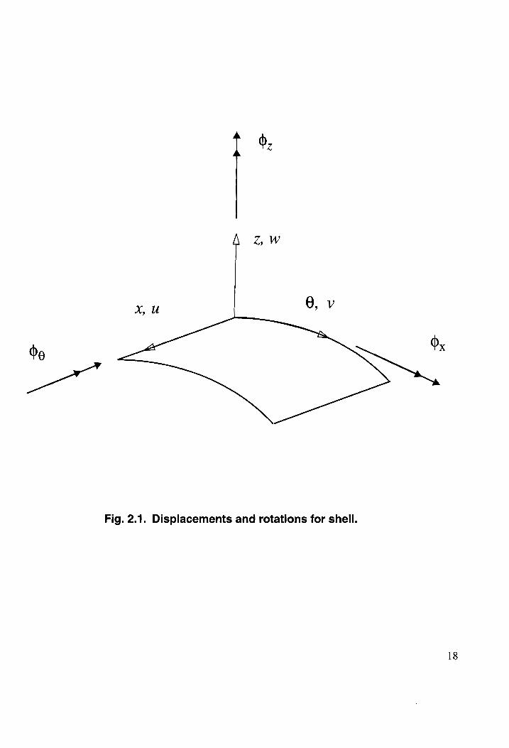
Fig. 2.1. Displacements and rotations for shell.

0

18

V(2,6,z) = v(z,0) + zde(z, 8) (2.2)

W(2,6,z) = w(2,8) (2.3)

where u(z,@), v(z,@) and w(z,@) are the displacements of the points of the reference

surface, and $;(z,0) and ¢¢(z,@) are the rotations of the normal to the reference surface

as shown in Fig. 2.1. Assuming small displacement gradients, the three-dimensional

engineering strains are related to the displacements by

OU 1 OV OW

eo = Go, 0 = Tey alogtW) te = GP (2-4) OV 1 ou

“t= Oe * (RFs) 00 (25) dU OW ov 1 OW

= = ort oe 6 = a taralae 1! (2.6) in which the polar radius r in cylindrical coordinates is replaced by R + z. Substituting

Eqs. (2.1) to (2.3) into Eqs. (2.4) to (2.6), and rearranging the terms results in the

following expressions for the three-dimensional engineering strains:

€66 + ZKae Crr = €ex t 2ZKx 699 = €s, = 0 (2.7)

wo tlt =5)Keg + Zhe érg = Yxre ( + op) 6+ oR 6 (2.8)

(1+ %)

Cez = YVrz Céz _162 (2.9) ~ O+%) in which €g7, Ker, €665 666, Yx@, Br, Kr6, Yrz, and yg, are the shell strains independent of z-

coordinate. These shell strains are defined in the following sub-subsection. The transverse

shear strains e,, and eg, given in Eqs. (2.9) were obtained through differentiation of Eqs.

(2.1) to (2.3) with respect to z However, Eqs. (2.1) to (2.3) are approximate in the

zcoordinate, so that differentiating with respect to z cannot capture the distribution

of the transverse shear strains through the thickness of the shell. Since the material is

19

assumed rigid in the z-direction (e,, = 0), the distribution of the transverse shear strains,

and consequently the distribution of the transverse shear stresses, does not influence the

shell behavior. It is the integral of the transverse shear stresses through the thickness,

or transverse shear resultants, that influences shell behavior. Thus, Eqs. (2.9) should be

viewed as average values of the transverse shear strains, or as the transverse shear strains

evaluated at the reference surface (z = 0).

2.2.1.1 STRAIN-DISPLACEMENT RELATIONS

In Eqs. (2.7) to (2.9), the two-dimensional, or shell, strain measures, which are

independent of the z-coordinate, are defined by

Ou Obr ‘cr = Op Nex = a

cg = oh B ag = OM RoO R R 06

Ov 10u 1x6 = 5 + Re

keg = 298 1 bx idv

Ox ROO ROL

Keg =< 200 LOGe _ 1 Ov

Oc R O6 ROz«

yer = be + SY yoo = oe 24 58

If we set the (average) transverse shear strains in Eqs.

rotations of the normal are

Ow br ~ On

v 1 Ow

= RRO

so that

—. . 2 Orw 2 Ov

Koo = Be RP acdd | ROL Kero = 0

(2.9) to zero,

(2.10)

(2.11)

(2.12)

(2.13)

(2.14)

(2.15)

then the

(2.16)

(2.17)

(2.18)

20

Hence, the thickness distribution of the shear strain reduces to

coy = 1b t 2 + aA) Kes (2.19) ° (1+ #)

24 which coincides with the results of Novozhilov’s** classical shell theory.

It is evident from Eq. (2.8) that three shell strain measures are needed to represent

the distribution of the in-plane shear strain through the thickness in the transverse shear

deformation shell theory. Whereas, only two shell strain measures are required in classical

shell theory to represent the shearing strain distribution through the thickness (refer to

Eq. (2.19)). Also it can be shown that under rigid body motions of the shell, the nine shell

strain measures, given by Eqs. (2.10) through (2.15) vanish. (For Novozhilov’s classical

shell theory, six shell strain measures given by Eqs. (2.10-2.12) and (2.18) vanish under

rigid body motions. )

2.2.1.2 VIRTUAL WORK

In the three-dimensional elasticity theory, the internal virtual work for the shell is

given by

bwener =/ff [Onrb€nx + 799599 + Fzz6€zz + Or96€xg + On26€rz + 0426€92| dV

(2.20)

where V denotes the volume of shell and dV = (1+ 4) dxR d@ dz. Substitute the variation

of Eqs. (2.7) to (2.9) into Eq. (2.20), and note that the virtual strains are explicit functions

of z. Integrals of the stresses with respect to z give force and moment resultants conjugate

to the shell strains. Hence, the volume integral in Eq. (2.20) reduces to an area integral,

and the internal virtual work becomes

é gael = II §@F on O shell dS, (2.21)

S

21

where S denotes the area of the reference surface with dS = dz Rd@. The generalized 9 x 1

stress vector for the shell in Eq. (2.21) is defined by

O shell = [Naw Noo, Nex, Merz, Moo, Mea, Meo, Qe, Qe’, (2.22)

and the generalized strain vector for the shell is

so _ T €shell = [eras 666, 20s Kar, 66, hnb, x65 nz, Oz) (2.23)

The physical stress resultants and stress couples for the shell, some of which appear in

Eq. (2.22), are defined in terms of stress components of the symmetric stress tensor in

cylindrical coordinates by

(Nez, Morr) = [0,2)o00(1 + =) dz t R

(Neo, Moa) = / (1,2)o%9 dz t

(Nz, Myo) = [0.200001 + 5) dz

: (2.24) (Noe, Moz) = fa. Z)Ogr dz

t

2: a2(l =) dz Qe = fo(1+ 5)

Qe = [oezde t

In Eq. (2.22), M9 and M,»9 are the mathematical quantities conjugate to the modified

twisting measures Kzg and K 9, respectively, and are defined in terms of the physical stress

couples by

— 1 ~ 1 Mee = 5 (Mee + Mor) Meo = 5 (Meo _ Moz) (2.25)

The nine elements of the stress vector in Eq. (2.22) and the relations of Eq. (2.25)

determine all the stress resultants and stress couples listed in Eq. (2.24) except for shear

resultant Ng. The shear stress resultant Nz» is determined from moment equilibrium

about the normal for an element of the shell. This so-called sixth equilibrium equation is

Mor

R Neo = Nor + (2.26)

22

Written out in full, the internal virtual work for the shell is given by

syehell / [ [Neo Seon + Noodcos + Nox626 + Mezbkiee + Moodtive + Myo bRve

+ Mz 9bk%ee + O26 Yarz + Q66702] dS

(2.27)

The external virtual work for the shell is

éweshell _— swerell 4 éwesrell (2.28)

where bwehell is the external virtual work due to the spatially uniform internal pressure

load, and 6W$""' is the external (or augmented) virtual work due to interacting loads.

The external virtual work for a cylindrical shell under uniform internal pressure, including

an axial load due to the closed-end effect, is written as

: RP | sywshell — [fe éwdS + »| =z 08 [5u(1,6) — 5u(—1, 8)] (2.29)

-@

The discussion on the augmented virtual work due to interacting loads is given in Section

2.0.

2.2.1.3 CONSTITUTIVE RELATIONS

The material law for an orthotropic lamina with one material axis in the normal

direction is given by

Orr Qu Qi2 Qi6 rx

Toe p= |Q12 Qa2 Qe] 4 €oe (2.30) Ox8 Qie Qee Qee] | exe

where Qi; are the transformed reduced stiffnesses given in the text by Jones?®. (The

thickness normal stress is assumed to be zero in the material law.) Substitution of Eq.

(2.30) into Eqs. (2.24) in conjunction with Eqs. (2.25), and use of Eqs. (2.7) to (2.9) for

the three-dimensional engineering strains, results in the following linear elastic constitutive

23

law for a laminated composite shell wall:

New Noe Nox

Moz Moe Mee

Mee

Ai. Aig Bir Bio Bile Big Ex Aso Agog Big Boo Big Bag E66 Aog Aces Ber Ber Bhe Bébe x6 By» Be Dy4 D2 Die D2, Ker (2.31)

Boo Bez Dig Da. Dig De K66

Big Bos Dig Dig Dee Dé6 Kind By, Bgs Dig D3 De Do§4 \ Kae

in which stiffnesses A;;,B;; and D;; are given by

(Aji, Bit, Dir) =/0. z,27)Qi(1+ = )dz

=|

(Ajo, Bio, Diz) = [022 \O12dz t

_ 2 ul

(A22, Baz, Doz) = [0,2.2)0n + @? dz t

(Aig, Bei) = [0,2)Qrede t

= 2.71

(A26, Ber) = [0.202601 + ? dz t

—1

Age = | Qeo(1 + 5) dz

Bi, =| G20 + 5)dz

Big = [ dw gpd (2.32)

Boe = [ One 4 3 + api + =) ‘dz

zal

d Bhy = [ Qavaal (1+ @) z

Bée = [ Qesz(1 + 55 + 5p + =) ‘dz

~ zi cl

Bég = | dee0 + RP dz

Die = [ Qw20 + sd

Dig = | dwipae

Dye = [ Qn + 5 + spl + a) ‘de

24

—i z Di, = | Qie5 (1+ ®) dz

zy -1 DE = | Ooo (+55 (+4) dz

_ zy -l Die = [ Qe + spl + PR? dz

z7l

Déé b= [ Ooo axl (1+ 5) dz

The lamina material law relating transverse shear stresses and strains is

Oxz Cag C45 | J Cxz = 2.33 O82 \ ci | ‘ €6z \ ( }

C44 = Gi13Cos’a + Go3Sin*a

C'45 =(Gi3 _ Go3)CosaSina

where

C's5 =G'93C 0s" a: + Gi35in?a

in which a is the ply orientation angle. Substitution of Eq. (2.33) into the last two of

Eqs. (2.24), in conjunction with Eqs. (2.9) for the transverse shear strains, results in

the following linear elastic constitutive law for a laminated composite shell wall relating

transverse shear resultants and strains:

3: } [as at | { T=} = 2.34

\ Q 6 Ags Ass | | Yoz (2.34)

The transverse shear stiffnesses, Ag4, A453, and Ass in Eq. (2.34) are given by

= 1 *)d Aga [cut + R? z

Ags = | Cosa (2.35)

t x -l

Ass = [ Css(1 +—) dz ! R

Since Eqs. (2.9) represent average values of the transverse shear strains, the constitu-

tive law relating transverse shear resultants and strains, Eq. (2.34), can be viewed as

25

a Hooke’s law based on the assumption of constant transverse shear strain distribution

through the thickness. Alternatively one can obtain the constitutive law relating trans-

verse shear resultants and strains based on the assumption of constant transverse shear

stress distribution through the thickness. A detailed discussion on the subject is given in

Chapter 2 of the text by Vasiliev?®. However, both the methods result in a shear correction

factor of one (as opposed to 5/6) for isotropic materials. Cohen?" derived the transverse

shear stiffnesses of laminated anisotropic shells without making either of the assumptions

mentioned above. He employed Castigliano’s theorem of least work to minimize the shear

strain energy, and obtained the desired constitutive law, which for homogeneous isotropic

materials gives a shear correction factor of 5/6.

2.2.14 EQUILIBRIUM EQUATIONS

The equilibrium equations for the shell can be derived using the principle of virtual

work which is stated as

awe” = ayysiel (2.36) for every kinematically admissible displacement field. For the purpose of deriving the

equilibrium equations of the shell, the contribution of the augmented virtual work due

to interacting loads is neglected in Eq. (2.28) for the external virtual work. Thus, sub-

stituting Eqs. (2.27) and (2.29) for internal and external virtual work, respectively, into

Eq. (2.36), using the definitions of the strain-displacement relations given by Eqs. (2.10)

through (2.15), performing integration by parts, and recognizing the arbitrary nature of

the first variation of the displacements, results in the following set of equilibrium equa-

tions, or Euler equations, for the shell:

ONg, | 1 ONor —_—_—_— + —

ae 37 éu Ae RP 96 0 (2.37)

ON xe 1 ONoe 1 _ éu;: Da R00 + Ree = 0 (2.38)

26

00+ 1a i Oe 100) It tp =0 (2.39)

ww: oe t ROO R

— OMzr | 1 OMez _ box : De + R 08.” Qe= (2.40)

OM 1 OMee _ bd6: De + R00 —Q,=0 (2.41)

2.2.15 BOUNDARY CONDITIONS

The derivation of Euler equations from the principle of virtual work results in the

following boundary integrals:

© : oR 41 ( re “> du + Negdv+ Qr6w + Mrrbds + Mrobds _# dé

-@ (2.42)

i +0

+ / | Noxdu + Ngodv + Qodw + Monddn + Meee] de =0 —l

Boundary integrals in Eq. (2.42) can be made to vanish individually by specifying the

boundary conditions in two ways. One way is to prescribe periodic boundary conditions;

alternatively either an essential or a natural boundary condition can be prescribed. In the

first case, the periodic boundary conditions at = +l are expressed as

Nzre(l,@) = Nee(—l, 8), dv(l,@) = dv(—l, 6)

Q,(1,@) = Q,(—1, 8), éw(l, 8) = dw(—l, 8)

(2.43)

M,,(1,@) = Mzz(-l, 8), 6¢(1,0) = d¢z(—I,@)

M,e(l,0) = Mzra(—l,?), 6he(1,0) = d¢e(-1,6) 6 € [-0,9]

For the closed-end pressure vessel effect, prescribe

R Nex(l,0) = pe and N,,(-1,6) = > 6 € [-0,0] (2.44)

27

Thus, 6u(+/,@) is not prescribed to vanish. Periodic conditions at 6 = +O edges are

Nor(2,0) = Nor(e,-9), éu(z,O) = du(z,-O)

Nee(z, 9) = Nog(x,-O), dv(z,O) = dv(a, -O)

Qe(z,0) = Qa(z, -9), 6w(z,0) = dw(z,-O) (2.45)

Moe(z,90) = Mee(z,-9), 6¢,(x,0) = 6¢,(2,-O)

Mor(z,0) = Mez(z,-9), 66(2,0) = d6ge(x,-9) we (-l,]|

In the second case, the associated boundary conditions at zc = tl edges are to

prescribe

either N,. — pe or u but not both,

either N,g or v but not both,

either Q, or w but not both,

either M,., or ¢, but not both, and

either M9 or dg but not both.

The associated boundary conditions at 9 = +O edges are to prescribe

either Ng, or u but not both,

either Ngg or v but not both,

either Qa or w but not both,

either Mg, or ¢; but not both, and

either Mgg or dg but not both.

2.2.2 STRINGER

Let us(z) and w.(2) denote the axial and normal displacements, respectively, of a

material point on the stringer reference axis, and let ¢g,(2) denote the rotation of normal

as shown in Fig. 2.2. Thus, the axial and normal displacements of a generic material

point of the stringer are given by

Us(2,€) = us(x) + €dos(2) (2.46)

28

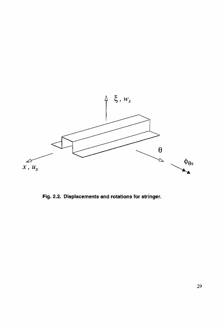
Fig. 2.2. Displacements and rotations for stringer.

gs

™

29

W,(2,€) = w.(z), (2.47)

respectively. The coordinate system (2,6, £) is located at the centroid of the stringer as per

the right-hand rule (see Fig. 2.2), in which € is the normal coordinate. Using Eqs. (2.46)

and (2.47) and assuming small displacement gradients, the three-dimensional engineering

strains are

§ s Cre = €as tEKos €3, = 0 €%, = Yes (2.48)

which are independent of the @-direction coordinate because of the symmetric deformation

assumption. In Eq. (2.48), the one-dimensional strain-displacement relations are defined

by

xs = U's Kos = 04s Yes = bos t+ W's (2.49)

in which €,, is the normal strain of the centroidal line, the product Ekg, is the portion of

the axial normal strain due to bending, y,, is the transverse shear strain, and the prime

denotes an ordinary derivative with respect to z.

The physical force and moment resultants for the stringer in terms of stress compo-

nents of the symmetric stress tensor are given, in usual way, by

(Nes, Mes) =f 008s dA,

Ves =/f o., dA, As

in which N,, is the axial force in the stringer, Mg, is the bending moment, V,, is the trans-

(2.50)

verse shear force, and A, is the cross-sectional area of the stringer. Based on transverse

shear deformation theory, the internal virtual work expression for the stringer is

i

bysiringer -/ [Nasb€xs + Mg,dKas + V256Yzs|dz, (2.51)

-1

and the Hooke’s law is

Nes = (EA) s€cs Mes = (ETI) s%es Vis = (GA) s¥z5 (2.52)

30

2.2.3 RING

The structural model is based on transverse shear deformation theory and includes

cross-sectional warping due to torsion. Warping is a distinctive feature of thin-walled,

open section beams. Restraint of cross-sectional warping, as occurs here in the ring

due to its contact with the shell, leads to additional longitudinal normal strains in the

ring as a result of torsion. The extension of classical thin-walled, open section, curved

bar theory to laminated composite materials was developed by Woodson, Johnson, and

Haftka?®. However, Woodson et al. did not consider transverse shear deformations. Most

of the developments for the ring theory presented here are obtained from Woodson’s

. . 9

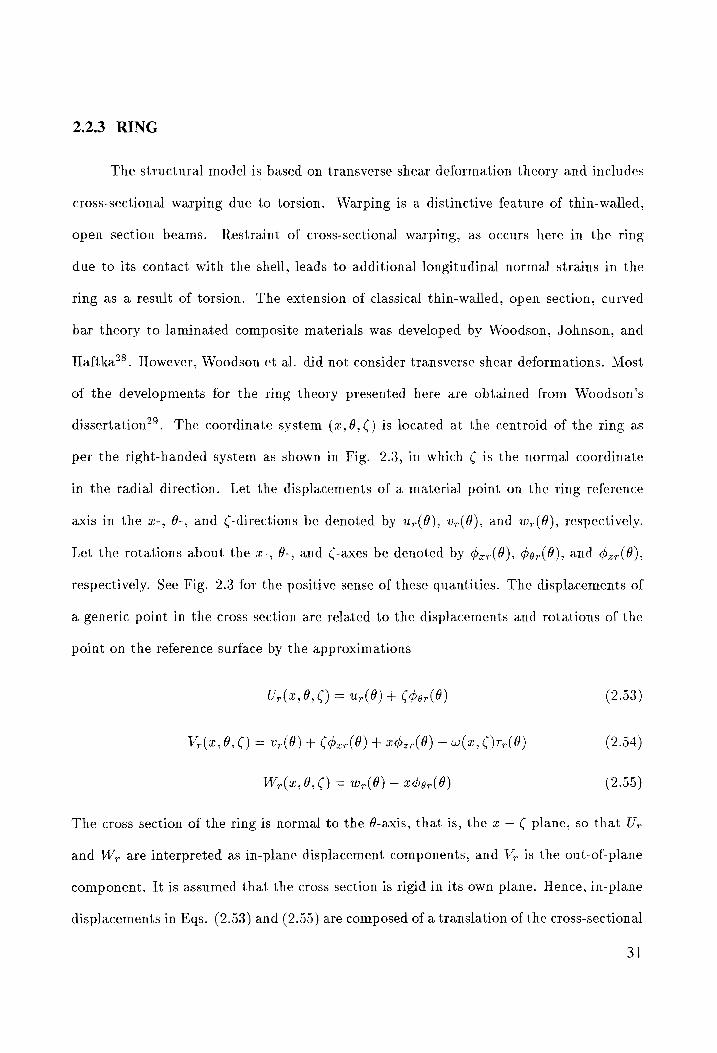
dissertation”? . The coordinate system (z,6,C) is located at the centroid of the ring as

per the right-handed system as shown in Fig. 2.3, in which ¢ is the normal coordinate

in the radial direction. Let the displacements of a material point on the ring reference

axis in the z-, @-, and ¢-directions be denoted by u,(@), v-(@), and w,(@), respectively.

Let the rotations about the z-, 6-, and ¢-axes be denoted by ¢,,(@), ¢9,(@), and $2,(8),

respectively. See Fig. 2.3 for the positive sense of these quantities. The displacements of

a generic point in the cross section are related to the displacements and rotations of the

point on the reference surface by the approximations

U,(@,0,C) = ur(8) + Cher(@) (2.53)

V,(@,8,0) = vr(8) + Cbor(9) + thzr(8) — w(2,C )Tr(8) (2.54)

W,(2,9,¢) = wr(@) — xdor(6) (2.55)

The cross section of the ring is normal to the @-axis, that is, the z — ¢ plane, so that U,

and W, are interpreted as in-plane displacement components, and V, is the out-of-plane

component. It is assumed that the cross section is rigid in its own plane. Hence, in-plane

displacements in Eqs. (2.53) and (2.55) are composed of a translation of the cross-sectional

3]

Fig. 2.3. Displacements and rotations for ring.

0g,

32

origin plus a small rigid body rotation ég, about the 6-axis. The out-of-plane displacement

given by Eq. (2.54) is composed of a translation of the origin v,, a component C¢z, due

to bending about the z-axis, a component x¢,, due to bending about the ¢-axis, and a

component —w7T, due to warping of the cross section out of the flexural plane. In Eq.

(2.54), w(x,¢) is the warping function for the ring’s cross section, and 7,(@) is the twist

rate which is given after the next equation. The internal virtual work is

Oo

swe = / [Nord€r + Morb Kap + MardKe2r + Ts76Tr + Mur6(Tr/ Ro) + Vor 6 Yar (2 56)

—~@ .

+ V.76Y27]Ro dé

in which No, is the circumferential force, M,, is the in-plane bending moment, M,, is the

out-of-plane bending moment, M,,, is the bimoment, 7, is the St. Venant’s torque, Vr,

is transverse shear force in the x-direction, V,, is transverse shear force in the ¢-direction,

€g, is the circumferential normal strain of the centroidal arc, Kz, is the in-plane bending

rotation gradient, «,, is the out-of-plane bending rotation gradient, y,, is the transverse

shear strain in z-@ plane, 7,; is the transverse shear strain in 6-¢ plane, and Ro is the

radius of ring reference arc. The rotations and strain-displacement relations are

1, 1. 1. Car = —(v, + Wr) Ker >= — er Ker = —( er _ er)

Ro Ro Ro oO ' (2.57) Tr = Re” + Per) Ver = Par _ Rye” _- Wp ) Yer = Pup + Ro

in which the over-dot denotes an ordinary derivative with respect to 6. The material law

is based on the assumption that the shear forces are decoupled from extension, bending,

and torsional deformations of the ring. Thus, Hooke’s law for the ring is

Nor EA ES, —-ES, —-#S, LH €or

Mop ES», Elyr —Elze -Eluy LA, Ker

Mp = —~ES, —-EI,, Elz: Ely, —FH, Ker , (2.58)

Mor -ES, -Elg, Ely: El, —-EH, Tr/ Ro

T sr BH EH, -EH, —EH, GJ Tr

and

Ver _ GAzg GAz: Yer ‘

| = an oa Ie } (2.59)

The stiffnesses in Eq. (2.58) are commonly referred to as modulus-weighted section

properties. The “EH” terms are unique to laminated thin-walled beams (see Bauld and

Tzeng*°). If the laminate construction for each branch of the ring is specially orthotropic

with respect to z-, @-, and ¢-directions, then the “EH” terms are all equal to zero. The

stiffness elements are evaluated from a computer code developed by Woodson. The reader

is encouraged to refer to Chapters 2 and 3 of Ref. [29] for further details on this subject.

The transverse shear stiffness elements in Eq. (2.59) are given by

K

GAs =[As5 hw + 5 (Ae )e (bw)a] k=1

K

GAz,z =[Ags hy + S (Aas Je (bw dx (2.60) k=1

K

GAzg =[Aos hw + S_(Ass)e (bw) a k=1

in which the transverse shear stiffnesses, A44, Aq3, and Ass are calculated based on the

assumption of constant transverse shear strain distribution through the thickness, and

are given by Eq. (2.35). In deriving the transverse shear stiffness elements given by Eqs.

(2.60) above, it is assumed that cross section of the ring is made up of a vertical web and

horizontal flanges. That is, the web is assumed to be parallel to the ¢-axis, and flanges

are assumed to be parallel to the z-axis. In Eqs. (2.60), the parameters h,, and b,, denote

the web height and flange width, respectively, and A is the total number of flanges in the

ring cross section.

For structural models in which the effect of warping of the ring cross section is

excluded, the contribution of the bimoment, M,,,, to the virtual work of the ring in Eq.

(2.56) is neglected, and the fourth row and column of the stiffness matrix, Eq. (2.58), are

ignored. Also, the warping function w(z,¢) is taken as zero.

34

2.3 CLASSICAL FORMULATIONS

2.3.1 SHELL

The shell is modeled with Sanders’ theory?!, in which first approximation thin shell

theory is used; i.e., the effects of transverse shear and normal strains are neglected. The

displacements at an arbitrary material point in the shell are approximated by Eqs. (2.1)

to (2.3), in which the rotations ¢, and ¢¢ are related to the displacements by Eqs. (2.16)

and (2.17), respectively. Thus, transverse shear strains e,, and eg, in Eqs. (2.9) vanish.

For small displacement gradients, the three-dimensional engineering strains in Sanders’

theory are given by Eqs. (2.7) and

2

Cro = (1+ am t+ FRe xe + 2(1 + sR) Kio

7 (1+ %) in which the quantity «3, is the twisting strain measure in the Sanders’ theory, which is

(2.61)

defined in the following sub-subsection.

2.3.1.1 STRAIN-DISPLACEMENT RELATIONS

Define a generalized strain vector in terms of the shell strain measures by

Esnell = [€xx,€80, ods Koa, KG0, Kee] (2.62)

The first five strain measures of the shell reference surface in Eq. (2.62) are related to the

displacements by Eqs. (2.10-2.12), and the sixth strain measure, K°,, is given by

» _ 06, 10b 1, = — —o, 2. “ee = Ge T ROO Re (2.65)

in which the rotation about the normal, ¢,, is given by

1,dv 1 0u 2=-(—--=s 2.64

? 2°0r R 50) (

The Donnell-Mushtari- Vlasov (DMV) approximation, or quasi-shallow shell theory is ob-

tained by neglecting the term % in Eq. (2.17) for the rotation ¢g, and the rotation about

the normal ¢, in Eq. (2.63).

35

2.3.1.2 VIRTUAL WORK

Define a generalized stress vector in terms of the stress resultants and couples of

Sanders’ theory by

Gsnew = (Nex, Noo, Nog, Max, Mog, M3,]* (2.65)

such that the internal virtual work is still given by Eq. (2.21) except that the stress

and strain vectors are 6 xX 1 vectors in Sanders theory. Quantities VN’, and M&, are the

modified shear and twisting moment resultants. In terms of physical stress and moment

resultants of the shell these are given by

1 1 9= = Nz Nez Tn £6 £ . Sp = 5( Nae + Noo) + o(Meo ~ Mex) (2.66)

3 1 6 5 (Mes + Moz) (2.67)

In the Sanders’ original paper*’ the term 7(Mze — Maz) in Eq. (2.66) was considered

to be small as compared to (Nzo + No,), and was, therefore, neglected. However, this

approximation is not made here. For infinitesimal virtual displacements, the internal

virtual work for the shell can be obtained by substituting Eqs. (2.62) and (2.65) into Eq.

(2.21), which results in

éwe9nell = iI [Naed€rat+ Noabdese t+ Negbyxo + MrrbKart+ Mogdkogt+ MigbK36| dS (2.68)

Ss

where S denotes the area of the reference surface. The external virtual work expression

for the classical shell theory is still given by Eq. (2.28).

2.3.1.3 CONSTITUTIVE RELATIONS

Consider the material law for an orthotropic lamina given by Eq. (2.30). To get the

material law for the shell, substitute Eq. (2.30) into the definitions of the resultants in

terms of stresses, Eqs. (2.24); substitute Eqs. (2.7) and (2.61) for the three-dimensional

36

strains; and then perform the integration with respect to the thickness coordinate. Using

the definitions of the modified resultants in Eqs. (2.66) and (2.67) gives the final form of

the material law as

Nee

Noe

Nie Morr Moe

Mere

Ai, Aig Are Bir Bio Bre Exe Ayo Ago Age Bip Boz Boag €66

_ |Ate Axe Ass Ber Ber Bee x6 (2.69) By By Ber Dir Dir Die} | kee By. Boo Ber Dio Doo Doe K66 Big Bop Bop Die Doe Dee Koo

where the stiffnesses Aj1, A1o, A22, Bir, Bi2, Boo, Diy, Dig and Doo in Eq. (2.69) are given

by the first three of E qs. (2.32), with the remaining stiffnesses defined by

: 2 (A16, Ber) = [2 )Qre[1 + 55 + vrei

(Age, Bez) = [a z)Q26(1 + SP + Sala + 5) dz

_ ~1 Age = | Qeoll + 5 + vt (1+ >) dz

Bie = | Qrox (1+ s5)d

- z-l _ Zvi. 2yE 2.70 Boe [G20 + 71e + R? d (2.70)

B ) z ar 66 = | Qeozlt + ‘aR * al * ap (1+ 5) Zz

2.3.2 STRINGER

D16 = [Que 4 + 5p)

~ gz. -l

D6 = | Grez*( + spill + ry dz t

Dee = [ Qsoz*( + 3 + =) (1+ a) a: t

The stringer is modeled with Euler-Bernoulli beam theory thereby neglecting the

transverse shear strain. Hence, equating yz, in the last of Eqs. (2.49) to zero results in

the following expression for $¢s:

6s = —w, (2.71) s

37

It may be noted that neglecting the transverse shear strain would also modify the virtual

work statement given by Eq. (2.51), and the third equation in the Hooke’s law, Eq. (2.52),

is neglected.

2.3.3 RING

The ring is modeled with thin-walled, open section, curved bar theory developed by

Woodson, Johnson, and Haftka?*. For classical formulations, the transverse shear strains

are neglected. Hence, equating y,, and y,, in the last two of Eqs. (2.57) to zero results

in the following expressions for the rotations ¢;, and zp.

1 Up — Wr) Pzr = —Z-Ur (2.72) Per = Ro =(

Ro

It may be noted that neglecting the transverse shear strains would also modify the virtual

work statement given by Eq. (2.56), and Hooke’s law for the shear resultants, Eq. (2.59),

is neglected.

2.4 DISPLACEMENT CONTINUITY

In order to maintain continuous deformation between the inside surface of the shell

and stiffeners along their lines of contact, the displacements and rotations should be

continuous at the shell-stiffener interface. For a symmetrical section stringer, the unit cell

model is symmetric about z-axis, and the only non-zero displacements for the stringer

are the axial and normal displacements. The axial and normal displacements at the top

flange of the stringer in contact with the shell are obtained from Eqs. (2.46) and (2.47)

for € = e,, where e, is the radial distance from the stringer centroid to the contact line

along the inside surface of the shell. Similarly, the corresponding shell displacements

at the inside surface of the shell (i.e., at z = —t/2) are obtained from Eqs. (2.1) and

38

(2.3). Hence, the following displacement continuity constraints are imposed along the

shell-stringer interface (i.e., -I<a2<l,@ = Q).

t Grs = U(z,0) - 7 Pele, 0) — [us(z) + esdos(z)| = 0 (2.73)

Gzs = wW(z,0) — w(x) = 0 (2.74)

The asymmetrical section ring bends out-of-plane and twists, in addition to in-plane

bending and stretching along its circumference. Hence, the displacement field for the ring

consists of axial, circumferential, and normal components given by Eqs. (2.53) to (2.55).

From Eqs. (2.54) and (2.55), it can be observed that the circumferential and normal

displacements of the ring vary along the width of the attachment flange.

Point-wise continuity of the circumferential displacement between the inside surface

of the shell and the attachment flange of the ring implies

V(2,0,—-t/2) = V,(2,0,e,) x € (—by1, 572), 6 € (-O,0) (2.75)

in which by, + bs. = by > 0 where 6; is the width of the attachment flange, and e, is

the distance from the ring reference arc to the contact line along the inside surface of the

shell. Since the kinematic assumptions in the ring theory give V, as an explicit linear

function of z, Eq. (2.54), and the z-distribution of the shell displacement V, Eq. (2.2), is

not known apriori, pointwise satisfaction of Eq. (2.75) across the width of the attachment

flange cannot be achieved. To proceed, the shell displacement is approximated in a Taylor

series in x about « = 0. That is,

OV 2 V(e,0,-t/2)= V(0,0,—t/2) + 25 le=o + O(2 } (2.76)

Substituting Eq. (2.76) into Eq. (2.75), the continuity of the circumferential displacement

across the width of the attachment flange can be achieved through terms of order x. Thus,

V(0,0,—t/2) = V,(0,@,e,) leads to

t Jor = (0,8) — 3 70(0, 9) — [v-(8) + erder(O) — woTr(@)] = 0, (2.77)

39

and r2¥|,-9 = V,(«,6,e,) — V-(0, 9, e,) leads to Ox

Ov t 0d¢

Ger= [Felco 2 Be _-0| — [Pzr(8) — wiry (8)] = 0 (2.78)

The constraint G,, = 0 imposed through Eq. (2.78) also implies that the rotation about

z-axis of the shell’s line element tangent to 2z-curve, Y equals the rotation of the ring

around ¢-axis along their contact line. In Eqs. (2.77) and (2.78), parameters wo and w

are the constant coefficients in the contour warping function, w(z,¢C) = wo + rw, for the

attachment flange of the ring. (Thickness warping is neglected and ¢ =constant along the

flange contour.) For structural models in which the effect of warping of the ring cross

section is excluded, the contour warping function w(z,¢) is taken as zero.

Similarly, point-wise continuity of the normal displacement between the inside sur-

face of the shell and the attachment flange of the ring implies

W(2,0,-t/2) = W,(2, 0, e,) t € (—by5i1, 072), 9 € (-O,0) (2.79)

Since the kinematic assumptions in the ring theory give W, as an explicit linear function

of z, Eq. (2.55), and the x-distribution of the shell displacement W, Eq. (2.3), is not

known apriori, pointwise satisfaction of Eq. (2.79) across the width of the attachment

flange cannot be achieved. To proceed, the shell displacement is approximated in a Taylor

series in x about x = 0. That is,

W (2,6, —t/2) = W(0,0, —t/2) + 0M 0 + O(a?) (2.80)

Substituting Eq. (2.80) into Eq. (2.79) the continuity of the normal displacement across

the width of the attachment flange can be achieved through terms of order x. Thus,

W (0,0, -t/2) = W,(0,6,e,) leads to

Jzr = w(0, 6) _ w,(8) = 0 (2.81)

40

and ee | <0 = W,(z,6,e,) — W,(0,6,e,) leads to

Ow Gor = Or | -o + Per(A) = 0 (2.82)

The constraint Gg, = 0 imposed through Eq. (2.82) also implies that the rotation about

§-axis of the shell’s line element tangent to z-curve, —3 is equal to the twist of the ring,

gor, along the contact line.

Point-wise continuity of the axial displacement between the inside surface of the

shell and the attachment flange of the ring implies

U(z,6, —t/2) = U,(z, 6, e,) x € (—by1, 572), 6 € (-0,0) (2.83)

Since the kinematic assumptions in the ring theory give U, independent of z, Eq. (2.53),

and the shell displacement U, Eq. (2.1), is an arbitrary function of 2, pointwise satisfaction

of Eq. (2.83) across the width of the attachment flange can be achieved only through terms

of order z°. Thus, U(0,6, —t/2) = U,(0,6,e,) leads to

. t ger = u(0,0) — 5 ox(0,8) — [ur(@) + erdor(8)| = 0 (2.84)

In order to include the axial load sharing between the shell and stringer due to closed-

end pressure vessel effects directly into the analysis, a seperate constraint is imposed. This

constraint is that the elongation of the shell at 6 = 0, z = 0 and the elongation of the

stringer at € = 0 are the same; i.e.

[U (i, 0,0) ~ U(—1,0,0)| 7 [Us(1, 0) ~ U;(—1,0)| = 0 (2.85)

Substituting Eqs. (2.1) and (2.46) into Eq. (2.85) leads to

[u(t,0) — u(-1,0)] — [us(1) - us(-))] = 0 (2.86)

4]

2.5 AUGMENTED VIRTUAL WORK FOR THE ASSEMBLY

Inter-element continuity is enforced by augmenting the virtual work functional with

the integrals of Lagrange multipliers functions times the variations in the displacement

constraints. Refering to Fig. 1.3 the Lagrange multipliers are interpreted as the compo-

nents of the interacting line loads between the stiffeners and the shell, and are defined

positive if acting on the inside surface of the shell in positive coordinate directions. Thus,

for the shell, the augmented (or external) virtual work due to the interacting loads is

syyeiell — | { rzo(2) [6u(e,0) — 5ode(2,0) + Asa(2)éw0(2,0)} dr -l

©

+ / {Azr(8) [ou(0, 8) ~ =642(0,8)] + Aar(A)[6(0, 4) ~ 56d(0, 6)| (2.87)

~o Ow Ov 0 + Aop(B)6w(0,8) — Nor(8)6( 5 |,-5) + Mer(A)6( S| ao ~ 5 pleco) }*

(R- 5)d0 ~ Q[éu(l,0) — 6u(—I,0)]

The axial force Q in Eq. (2.87) is an additional Lagrange multiplier that accounts for axial

load sharing between the stringer and shell. Similarly, for the stringer, the augmented (or

external) virtual work due to the interacting loads is

i

gyystringer __ | {Azo(2) [Su4(2) + esdh6s(2)| 4 Az9(2)bw,(2)} dz J, (2.88)

+ Q[6u.(1) — bus(—J)]

and, for the ring is given by

©

bwers = -| { Avr(8) [Sur(8) + €rddor(O)| + Agr(O)[6v,(8) + erdder(9) — wodTr(B)|

-0

+ Asr(B)8we(8) + Nor(0)8der(#) + Aar(8) [6Gze(8) ~ ur 67-(8)] J+ po)

Ro dO (2.89)

42

The displacement constraints (Eqs. (2.73), (2.74), (2.77), (2.78), (2.81), (2.82),

(2.84) and (2.86)) are enforced by vanishing of the inner product of these equations with

the variations in the Lagrange multiplier functions. The variational form of these con-

straints are

J (reedos + Odeegee] de = 0 (2.90) “)

oe

/ [Orr Gar + 6X 6rGer + OX2rJzr + 6AgrG6r + bAzrGzr| (Ro + er) d@ = 0 (2.91)

-O

6Q{ [u(l,0) — u(—I,0)] - [us(2) - us(-D]} = 0 (2.92)

43

CHAPTER 3

GOVERNING EQUATIONS FOR NONLINEAR ANALYSIS

3.1 ANALYTICAL MODEL AND ASSUMPTIONS

A geometrically nonlinear elastic analysis is carried out for the orthogonally-stiffened

cylindrical shell subjected to internal pressure. The structural repeating unit (or unit cell

model) of Fig. 1.2 is analyzed to obtain response of the entire structure. The shell is

modeled with Sander’s nonlinear theory of thin shells, and the stiffeners are modeled with

a nonlinear Euler-Bernoulli beam theory. The purpose of nonlinear elastic analysis is

twofold: First, the distributions of interacting loads between the shell wall and the stiff

eners are obtained and compared with those obtained from a geometrically linear elastic

analysis. Second, the influence of geometric nonlinearity on the the stress concentration

in the shell adjacent to the stiffeners due to “pillowing” is studied.

Only stiffeners with symmetrical cross sections are considered for the nonlinear re-

sponse. Hence there is no out-of-plane bending and torsion of the ring, and no rotation of

the joint at the stiffener intersection about the circumferential axis. Also, on the basis of

the symmetry about the z- and 6-axes for the repeating unit, only the interacting line load

components tangent and normal to the stiffeners are included in the analysis. The shell-

stringer interacting force components per unit length along the contact lines are denoted

by Axs(x) for the component tangent to the stringer, and A,,(2) for the component normal

to the stringer. The two shell-ring interacting load components per unit length along the

contact lines are denoted by A9,(@) for the component tangent to the ring and 4,,(@) for

the component normal to the ring. These interacting loads acting in a positive sense on

the inside surface of the shell are shown in Fig. 1.3. In this chapter nonlinear formulations

44

are presented for the shell and stiffeners based on classical theory. The following general

assumptions are made for nonlinear elastic analysis of the repeating unit:

1. Normals to the undeformed reference surface remain straight and normal

to the deformed reference surface, and are inextensional.

2. Material behavior is linearly elastic.

3. The thickness normal stress is assumed to be small with respect to the normal

stresses in the axial and circumferential directions, and hence it is neglected

in the material law.

3.2 SHELL

3.2.1 STRAIN-DISPLACEMENT RELATIONS

Sanders*? nonlinear theory of thin shells is employed to model the shell. The gen-

eralized strain vector for the shell is given by Eq. (2.62). Assuming the strains are small

and rotations are moderately small, the membrane strain-displacement relations are

Ou ly lia

lov w 1, Il 66 = poe + R + 5% - 5%: (3.1)

Ov 10u Yr = aa Rae 1 oe

in which the rotations ¢,, dg and ¢, are given by Eqs. (2.16), (2.17) and (2.64), respec-

tively. The change in the normal curvature components, Krzr, Keg, and K%, in terms of the

shell rotations are linear and are given by Eqs. (2.10), (2.11) and (2.63), respectively. The

Donnell-Mushtari-Vlasov (DMV) approximation, or quasi-shallow shell theory, is obtained

by neglecting the rotation about the normal in the strains of Eqs. (3.1) and (2.63), and

45

the term % in rotation ¢g of Eq. (2.17). In this work, it is assumed that the contribution

of the rotation about the normal to the strains is negligible for the shell. However, the

DMV approximation is not assumed initially.

3.2.2 INTERNAL VIRTUAL WORK

The generalized stress vector in terms of the stress resultants and couples of Sanders’

theory is defined by Eq. (2.65), and the internal virtual work for the shell in deformed

state is given by Eq. (2.68). However, the stress resultants and stress couples are now

defined in terms of second Piola-Kirchhoff stress tensor, which is based on the undeformed

configuration of the body. Substituting for strains from Eqs. (3.1), Krzr from (2.10), Keg

from (2.11), and «2, from (2.63) into Eq. (2.68), in conjuction with Eqs. (2.16) and (2.17)

for the definitions of rotations, results in the following expression for the internal virtual

work for the shell:

oe = ff fe 0 Be a [BE MOM 1 [Ns oF (o" "4 ee 4 wel 5 (oe yee bw — Mex (8)

=e I 4 4 Pc (28 = 29 rs

Tape we ae) Ca} (3.2)

3.2.3 EXTERNAL VIRTUAL WORK

Mathematically the stiffened shell is considered closed at x = too. The work done

by hydrostatic pressure on an enclosed volume can be derived from a potential energy

functional, since hydrostatic pressure is a conservative load. However, the infinite volume

is inconvenient to deal with. Instead, a repeating volume element of the structure that is

of finite size can be considered, and the potential energy functional for it can be derived.

46

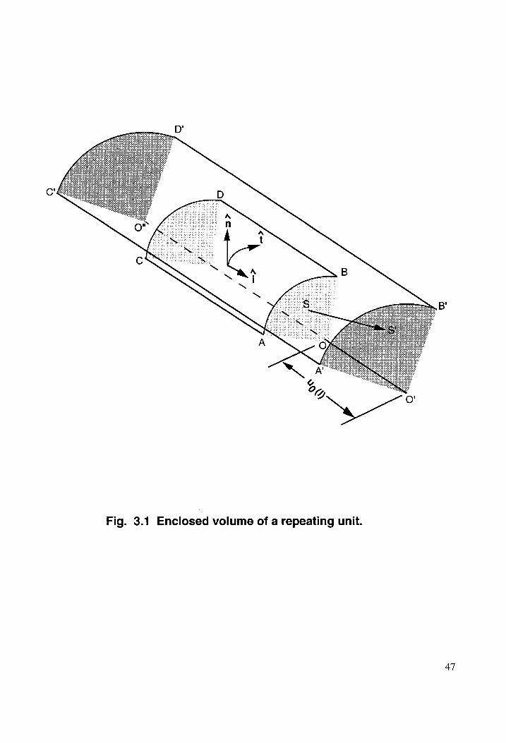
Fig. 3.1 Enclosed volume of a repeating unit.

47

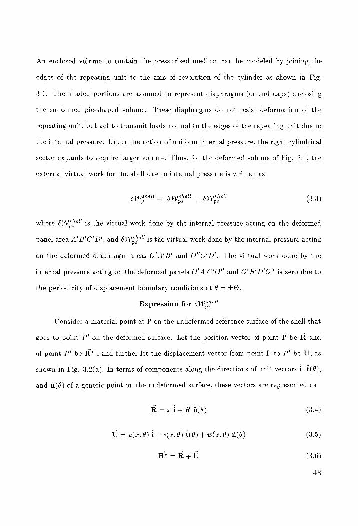
An enclosed volume to contain the pressurized medium can be modeled by joining the

edges of the repeating unit to the axis of revolution of the cylinder as shown in Fig.

3.1. The shaded portions are assumed to represent diaphragms (or end caps) enclosing

the so-formed pie-shaped volume. These diaphragms do not resist deformation of the

repeating unit, but act to transmit loads normal to the edges of the repeating unit due to

the internal pressure. Under the action of uniform internal pressure, the right cylindrical

sector expands to acquire larger volume. Thus, for the deformed volume of Fig. 3.1, the

external virtual work for the shell due to internal pressure is written as

hell hell hell bw = OWoee + OW (3.3)

where bwesnel is the virtual work done by the internal pressure acting on the deformed

panel area A’ B'C’D’, and bw is the virtual work done by the internal pressure acting

on the deformed diaphragm areas O’A’B’ and O”C"D’. The virtual work done by the

internal pressure acting on the deformed panels O’ A’C’O” and O'B'D'O" is zero due to

the periodicity of displacement boundary conditions at @ = +0.

Expression for bwerel

Consider a material point at P on the undeformed reference surface of the shell that

goes to point P’ on the deformed surface. Let the position vector of point P be R and

of point P' be R* , and further let the displacement vector from point P to P’ be U, as

shown in Fig. 3.2(a). In terms of components along the directions of unit vectors i, (6),

and n(@) of a generic point on the undeformed surface, these vectors are represented as

R=2ci+R n(é) (3.4)

U = u(x, 0) i+ v(a,9) t(0) + w(2, 8) a(9) (3.5)

R*=R+U (3.6)

48

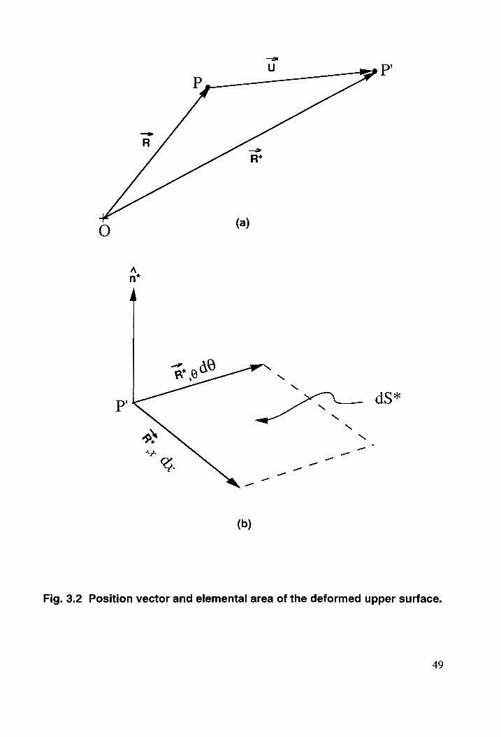
cy

P'

Dy

O (a)

=>

Fig. 3.2 Position vector and elemental area of the deformed upper surface.

49

Using the geometric property of the cross products of position vectors (Fig. 3.2(b)), an

elemental area dS* of the deformed surface can be written as

. aR* aR* ds* n* = —— —_—- ot o* n Dn dz x a0 dé (3.7)

where n* is the unit vector normal to the deformed surface element. Substituting Eqs.

(3.4) and (3.5) into Eq. (3.6), using the resulting expression for R* in Eq. (3.7), and

noting that au = t and at = —n, the following expression for the elemental area of the

deformed surface is obtained. “a

i dS*n* =|1+ 2

roe | l+Rl3e ew) RS where dS = Rdé@ dz is the elemental area of the undeformed surface. For the hydrostatic

n

w dS (3.8) Or

Ww pe|>

seh

ai

Oo

pressure p acting on the deformed surface A’ B’C’D', the external virtual work is given by

dwehell — |[_© dS* n*) e 6U (3.9)

where 6U = 6u(x,0) 1+ dv(a, 0) £(0) + 6w(x,@) A(@) is the virtual (infinitesimal) displace-

ment vector, and S* is the area of the deformed reference surface. Upon substituting Eq.

(3.8) into Eq. (3.9) and carrying out the algebra, the following expression for the first

component of external virtual work is obtained:

ows =e [AR Ge ge + le +N al Liege a8 a0 , , OU Ou 1 ,Ov 1 Ou Ov ~v) (1+ 24) oo4 [4 4) f+ 2H + wy] - Se] ow} ds

(3.10)

in which S denotes the area of the undeformed reference surface. Equation (3.10) is

expanded and the terms are rearranged to obtain the following intermediate expression

for the first pone of external virtual work:

1 Ov Ow WwW. . awshel =p [f {ols p(o? + wy. + 52+ w5e + gag) tu) ~ Gel + Hee 1 edu_de00), 1 (dwdu dws, , 1 (dudv _ du dv,

+ Blan 90 7 30 2)" * Bde 00 00 Oa R\d2 00 30 da 1. 9 9 Ou v Ov w,,0v, 1 dw ~ [ppv + w?) + w] 65) — 55-8 - Bh 55) — Bae éubas an

50

The terms containing derivatives of the virtual displacements in Eq. (3.11) are integrated

by parts, and then the terms are further rearranged to obtain the following expression for

the first component of external virtual work functional:

Ou 1 dv 1 ,dvdOw OAvdw 6 shell __ IT ls 2 “ ae fees Mea

Woe =P Pf Slap Fw)L+S =) +52 + R59) + aR Ga 00 BB ae) UT ded dey 1 (Quon _ Ou dv

38R\dOr 06 800 Oz 3R‘\dz 06 00 0x i

+e] (5leae Par] et [wt Ge ege)] & =!

+ [vee - aad sw} da ©

w + w| as

Ox -©

1 Ow Ov 1 Ou

rr f{[- wm ap ew) + ap (Gg 5p) | 8+ ap (eG -©

Ow 1 Ov Ou +!

wl

Expression for bwesien

The stiffened shell has a periodic symmetry about its axis of revolution in the sense

that a rotation of the structure through integer multiplies of 20 brings the structure into

self-coincidence. That is, after a rotation through 20 about the axis of revolution the

stiffened shell is indistinguishable from its original position. Since the pressure load is

spatially uniform, the deformed structure exhibits the same periodic symmetry about the

axis of revolution. That is, a rotation of the deformed stiffened shell through an integer

multiple of 20 about the axis of revolution brings the deformed shell into self-coincidence.

The @-curves of the shell’s reference surface at x = +/, both in undeformed and

deformed states, serve to define the end diaphragms. In the undeformed state the @-curves

are circles and the end diaphragms are circular areas of radius R. The diaphragms in the

deformed state are defined by the displacement of diametrical lines. Deformed images

of diametrical lines remain straight and pass through the axis of revolution. Consider a

51

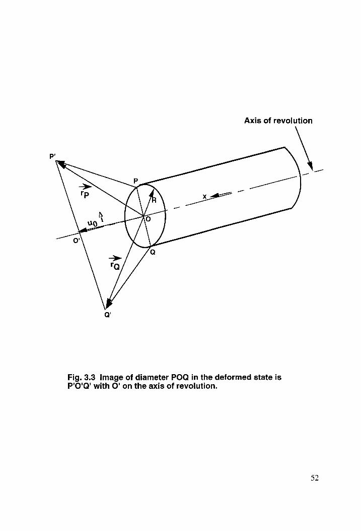
Axis of revolution

Fig. 3.3 Image of diameter POQ in the deformed state is P'O'Q' with O' on the axis of revolution.

52

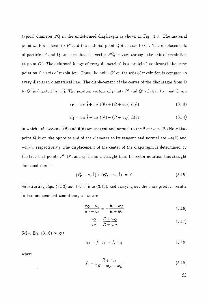
typical diameter PQ in the undeformed diaphragm as shown in Fig. 3.3. The material

point at P displaces to P’ and the material point Q displaces to Q’. The displacements

of particles P and Q are such that the vector P‘Q! passes through the axis of revolution

at point O’. The deformed image of every diametrical is a straight line through the same

point on the axis of revolution. Thus, the point O’ on the axis of revolution is common to

every displaced diametrical line. The displacement of the center of the diaphragm from O

to O' is denoted by uoi. The position vectors of points P’ and Q’ relative to point O are

rp = up it vp t(0)+(R+ wp) ald) (3.13)

rQ = ug i— vg t(6) — (R+ wa) ald) (3.14)

in which unit vectors t(@) and n(@) are tangent and normal to the @-curve at P. (Note that

point Q is on the opposite end of the diameter so its tangent and normal are —t(@) and

—n(@), respectively.) The displacement of the center of the diaphragm is determined by

the fact that points P’, O', and Q’ lie on a straight line. In vector notation this straight

line condition is

(rp — uo i) x (rQ — uo i) = 0 (3.15)

Substituting Eqs. (3.13) and (3.14) into (3.15), and carrying out the cross product results

in two independent conditions, which are

ug-—u _ k+we

upaty ~~ RF wp 6.16) 2 _ ot (3.17)

Solve Eq. (3.16) to get

uo = fi up t+ fe ug (3.18)

where

A= Reo ae (3.19)

53

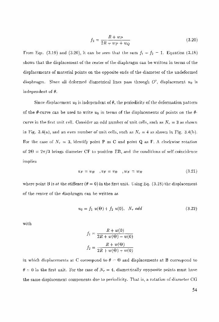
R+wp = 3.20

2h +wpt+ wo ( ) fo

From Eqs. (3.19) and (3.20), it can be seen that the sum f; + fg = 1. Equation (3.18)

shows that the displacement of the center of the diaphragm can be written in terms of the

displacements of material points on the opposite ends of the diameter of the undeformed

diaphragm. Since all deformed diametrical lines pass through O’, displacement uo is

independent of @.

Since displacement uo is independent of 6, the periodicity of the deformation pattern

of the @-curve can be used to write wo in terms of the displacements of points on the 6-

curve in the first unit cell. Consider an odd number of unit cells, such as NV, = 3 as shown

in Fig. 3.4(a), and an even number of unit cells, such as N,; = 4 as shown in Fig. 3.4(b).

For the case of N, = 3, identify point P as C and point Q as F. A clockwise rotation

of 20 = 27/3 brings diameter CF to position EB, and the conditions of self-coincidence

implies

UF =Up ,UF=vUB ,WRF=wB (3.21)

where point B is at the stiffener (9 = 0) in the first unit. Using Eq. (3.18) the displacement

of the center of the diaphragm can be written as

u=fhi u(O) + fo u(0), N, odd (3.22)

with

_ R+w(0)

N= 3Ry w(O) + w(0)

R+w(9) h= 2R + w(O) + w(0)

in which displacements at C correspond to @ = © and displacements at B correspond to

6 = O in the first unit. For the case of N, = 4, diametrically oppposite points must have

the same displacement components due to periodicity. That is, a rotation of diameter CG

54

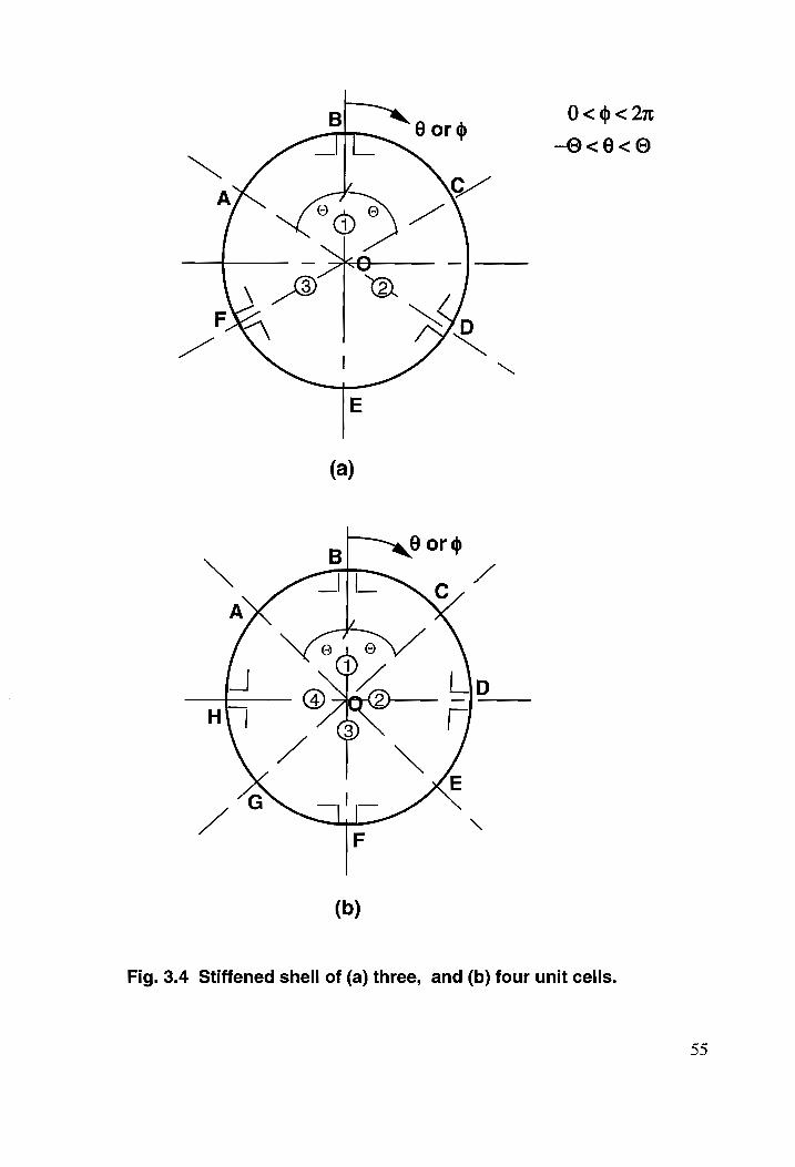
(b)

Fig. 3.4 Stiffened shell of (a) three, and (b) four unit cells.

55

in Fig. 3.4(b) through N,/2 multiples of 20, i.e., 7 radians, implies uc = ug, vc = VG,

and wo = we, with @ = © for point C in the first unit. Identify points C and G with

P and Q, respectively, in Eq. (3.18) such that the periodicity condition gives up = u(Q).

Similar considerations for diameter BF connecting the two stringers leads to up = u(0).

Therefore, for even number of unit cells one gets

uo = u(O) = u(0), N, even (3.23)

The condition for displacement up for N, odd is more complex than for N, even.

Consider a point $ in the circular sector OAB of the diaphragm at 2 = / as shown

in Fig. 3.1. The polar coordinates of S are r and @ withO<r< Rand -O<6< 0.

The particle at S displaces to point 5’ in the deformation. The position vector of point

5’ relative to point O is

r*(l,r,0) =r n(@) + a(l,r, 6) (3.24)

in which r n(@) is the position vector of point S, and u(/,r,@) is the displacement vector

of S. Since the deformed image of a diameter is a straight line, the displacement vector

for point S can be interpolated by

wi(L,7, 8) = = [u(t,8) 1+ o(1,6) (0) + w(l,8) A(@)] + (1 — Zuo!) i (3.25)

in which uo(!) is the axial displacement of the center of the diaphragm at x = /, and

it is given by Eq. (3.22) if N, is odd and Eq. (3.23) if N, is even. At r = #& the

displacement vector for the diaphragm coincides with displacement vector of the shell’s

reference surface at x = 1. The virtual work of the pressure acting on the deformed

diaphragm O'A'B' referenced to the undeformed diaphragm OAB is

Or* Or* ap dO x ar dr)

OR

at r=l -/ P ( -9 0

shell sei

, ¢ bail, 7, 8) (3.26)

56

Substituting Eqs. (3.24) and (3.25) into Eq. (3.26) results in the following expression for

the internal virtual work.

OR 640 +R (1,4) _ 6uo| sév Sé6w éwesnel _ [ou wen 1 2, dr dé at vel = P 1 iv V+ Rog + ¥) ne — ”) rar

-0 0 Alu ,9) — uo] R It Re |rnt (3.27)

A similar procedure is used on the circular sector of the undeformed diaphragm at

z = —l. Note that the displacement of the center of the diaphragm at 7 = —/ is uo(—1),

and it is given by either Eq. (3.22) or Eq. (3.23) as long as the displacements of the

é-curve at x = —/ are used in these formulas. The external virtual work of the hydrostatic

pressure on the deformed sector O"C'D’' is

OR

or* Or* Shell _ ay

Wd at x=-l i [fe ( o@ dé x Or dr) ° éu( lr, 6) (3.28)

-0 0

where / is replaced by -/ in Eqs. (3.24) and (3.25). The total external virtual work of the

pressure on the diaphragms is the sum of the virtual work of the pressure on each of them.

Expanding the determinate in Eq. (3.27) and performing integration with respect to polar

radius r (since r appears explicitly in the integrand), and following a similar procedure for

the virtual work done by the pressure acting on the end diaphragm O"C’D' (Eq. (3.28)),

the second component of the external virtual work is written as

°

shell _ + 1 ov, Ow Ov é6Woa p [Rees (v? + w')+ 5 (wae 0) + Sa] G bu + 260)

1 ;,Ow Ou + xg l( ag ~ 2) (uo) ~ Fal + w)| 60 1; Ou Ov +

4 sale va ~ (u-u uo) (R+ w+ =)| wh Rae

(3.29)

The total external virtual work for the shell due to internal pressure can now be

obtained by substituting Eqs. (3.12) and (3.29) into Eq. (3.3). In this substitution process,

57

the line integrals at edges x = +/ from Eqs. (3.12) and (3.29) combine and simplify.

(Several terms combine to add to zero, and integration by parts in @ are performed to

eliminate derivatives of the virtual displacements. Periodicity of the displacements at

6 = +0 result in vanishing of the boundary terms in the integration by parts.) After

these manipulations, the following expression for the total external virtual work for shell

results:

sett <p [fo] Apu? a tyr 4 2%) 4 (Ot 4 120), 1 (Bo dw dv dw OW, =» ff 6 sR +w)\l+ 5+ 05 + ge) + aR (Ge on 7 D0 De)”

! 1 ,0wdu OQwdu 1 ,dudv Oudv w+wlds+p/ {5| Ov

+ 3p (S530 ~ BO da)” + 3B da db” OO Da? wre 3 -l

— oS) é6u t+ | — w+ 5 (use - ty) go 4 [oot — ye) éw) de Ox Ox Oa 31l Oz Ox -9

e Ov.u Uo 1 Ov Ow

-@ 41

_ [5 + ale +4 w’))(u _ 0) R w|

” (3.30)

On the basis of periodicity of the shell’s displacements at 9 = +0 edges, it can be shown

that the first of the line integrals in Eq. (3.30) vanishes, and the final result for the

external work functional for the shell under hydrostatic pressure is

shell _ eee Ou Ou 1d. 1 dvdw dvdw Went =r] f [w+ sae + wilt 5o)+ wae + 259) + aR Ge Oo ~ Bde)"

1 ,dwdu Owdu 1 ,0dudv Oudv

xh (ac00 7 a0 a0) * Rae a0 ~ Bean)” *S ©

+ op f (e+ G+ B+ ylwgy egy) - .

_ [5 4+ ale” + w’)|(u- 7)

(3.31)

58

3.3 STRINGER

For a symmetrical cross section, the internal virtual work statement for the stringer

is l

6ywsiringer = [ecb + Mas6Ko5\dx (3.32) int

—l

in which N,, is the axial force in the stringer, Ms, is the bending moment, €z, is the

extensional normal strain of the centroidal line, and kg, is the change in curvature of the

centroidal line. Based on Euler-Bernoulli nonlinear beam theory, the strain-displacement

relations for stringer are

f i y2 a Eys = Us t 5 (ws) Kos = — UW, (3.33)

in which the prime denotes an ordinary derivative with respect to z. Substituting Eq.

(3.33) into Eq. (3.32) results in the following expression for internal virtual work for the

stringer.

0 0 0 a bWing we" = / [Nes (5 *) + Nes 5( an) — Mos 6( aah) dx (3.34)

~I

Hooke’s law for the stringer is

Nos = (EA) sts Mos = (ED) hes (3.35)

3.4 RING

For a ring with symmetrical cross section, there is no out-of-plane bending and

torsion. Hence, the statement of internal virtual work for the ring is

int

oO

~o

59

in which N¢, is the circumferential force, M,, is the bending moment, €g, is the circum-

ferential normal strain of the reference arc, Kz, is the change in curvature of the reference

arc, and Ao is the radius of ring reference arc. Based on small strains and moderate

rotations, and the kinematic relations for the ring are

lor = (0, + wr) + str

] Kar =p — dor (3.37)

Der =F(0 _ Wr)

in which the over-dot denotes an ordinary derivative with respect to #. Substituting Eqs.

(3.37) into Eq. (3.36) results in the following expression for internal virtual work for the

ring:

© ir Nor 1 Ow, No Ov Neo 6 ing __ ~ vr oF r r + Yor

Wint -| ‘ Ro (Fr Ro Oe =) év, + mo e a gt Ro 6Wp

-O (3.38)

Nor, 1 OWp Up Ow, OW,

Ro (Ro 00 80 ~ Ry) (SD -F Gar} Bo a

Hooke’s law for the ring is

Nor = (EA)r€6r Mop = (ELD) pK gr (3.39)

3.5 INCREMENTAL VIRTUAL WORK

The internal and external virtual work functionals obtained above contain terms

that are nonlinear in the displacements times virtual displacements of the first degree.

Newton’s method is employed to solve the nonlinear equilibrium equations that result

from the principle of virtual work. It is convenient to derive the incremental virtual

work functionals for each structural element for implementation of the update procedure

in Newton’s method. At fixed values of external loads, consider replacing the (actual)

60

displacement field in the virtual work functional of an element by an approximation. Let

this approximation be a known displacement field plus a small incremental displacement

field. The approximation is substituted into the virtual work functional of the element and

the functional is linearized in the incremental displacement field. As an example of the

replacement procedure, the case of shell is explained in detail. Let the shell displacement

field

{u} —> {ua} + {Au} (3.40)

in which {u} on the right hand side of Eq. (3.40) is assumed to be known and {Au} is

an unknown small increment. As a result of replacement illustrated by Eq. (3.40), the

strains and curvatures become

{é} —> {e} + {Ae} (3.41)

{k} —> {KE} + {AR} (3.42)

in which {Aé} and {Ak} are linear in {Att}. The stress and moment resultants are

replaced as

{N} — {N} + {AN} (3.43)

{M} — {M} + {AM} (3.44)

in which {AN} and {AM} are determined by the constitutive law (Eq. (2.69)) by using

incremental strains and curvatures; viz., {Aé} and {Ag}.

The virtual displacements are not incremented since they are any of a set of kine-

matically admissible (test) functions and it is only the (actual) displacements (in the space

of trial functions) that are being determined by iteration. Consequently,

§ (Ai) = 0 (3.45)

61

Substituting the replacements (Eqs. (3.40) through (3.44)) in the virtual work functional

(Eq. (3.2) or (3.30)), and linearizing in the increments results in the incremental virtual

work functionals. The above procedure is repeated for the stiffeners as well to obtain

respective incremental virtual work functionals.

3.5.1 SHELL

The linearized incremental strains and curvatures for shell are obtained by following

the incremental procedure described above. Substituting Eq. (3.40) to (3.42) into Eqs.

(3.1), (2.10), (2.11), and (2.63) in conjunction with Eqs. (2.16) and (2.17), results in the

following linearized incremental strains and curvatures for shell:

OAu Ow. OAw

Aer = Ge t+ (aay? 10Av Aw 1 Ow v. 1d0Aw Av

Acoo= Roe + Re tebe 7 RR G7 RB? (3.47) OAv 10Au OAw. 10w v Ow. 10Aw Av

(3.46)

Si = oy + Roe toe) Rae RT Se) RGR? MS) 2

Aker = = (3.49) 2

Akos = — a ag + aoe (3.50) 2

ee B a00 * BOs (an Similarly following the replacement procedure explained above, from Eq. (3.2) the lin-

earized incremental internal virtual work for the shell is obtained as

O ANS, 0 AN 10 AN, 0 b(AWwenelty = [ [amen 5) + Ee - 06 — —) + rg OW

Ss L v

R ‘RoO R kR a

- a iba) * ete tcomita » ait Av OAw

Ow ANgg,1 Ow v ANoe Ow

~ a) + Neo Ge Ja.) + | R rT R) +R be 4 Nes OAw Nog ,1 0Aw Ay) «(2 «(oe =)

R a2 + RR ob 7 RB a3,

and from Eq. (3.30), the linearized incremental external virtual work for the shell due to

internal pressure load is obtained as

shell | dAv Ow _ OAv Ow Ov OAw Ov OAw

(AW, 7 Seta dr Oe o dc | Oz 08. 00 Oz | éu+ | Aw

Ov pone OAv Ow Ou

‘ OAw >» Ow OAv Ou Av Ou

1 Ge a ae Oe | 65g) + [Fp + 5p) 42 ot 1 (eon dAw du | Ow Au _ ou OA)

R Oz dz 00 00 dx Ox 00 06 dx’! ow. pone OAw Aw 1 OAu

+ 5p [Augy - © ot ag sage) + [Fe + 3p (5, Ow Ou one w, oAu Ou, Aw ~A A 142)" ony aw "op Oar On apt (A+ gat 0+ 5)

ai OO tae (ee ee ee ey 5

R00 dz 00. 00 dc Ox 00 00 dz °

Ou OAv OAu Ov) ., Ow 1 Ov OAu

+ sp lA ag "56 1° 86 — Aus |6( 5) + ag Auge -° Oa 6

OAv Ou) .,Ow 1 OAv Ow $us — Ave “6 55)} ds + 8p la | (we - Ave

~@

Ov 0Aw Ov Ow OAv,u uo

+ Awag — va p-)uo + (wag — vay) Awe + Seg + F) Ov, Au Aug Aw 1

w 14 9 +! _ Fs + oR” +w*)|(Au— Auo)| R ao}

(3.53)

It may be noted that Eq. (3.53) leads to a symmetric load stiffness since constant pressure

acting on a fully enclosed volume is a conservative force system.

3.5.2 STRINGER

Following the incremental replacement procedure Eq. (3.33) results in the following

linearized incremental strains and curvatures for the stringer:

OAUs Ow, O0AWs +

Atos = Ox (Sy Ox ) (3.54)

63

07 Aw, a (3.55) Akers i

Simularly, from Eq. (3.34) the linearized incremental internal virtual work for the stringer

is obtained as

l

acawvsnrinee) = [ [Nes 6S) + (ANas Re? + Nowa) (SE) Ox Ox Ox Ox 2, (3.56)

Ow,

3.5.3 RING

The application of incremental replacement procedure to Eq. (3.37) results in the

following linearized incremental strains and curvatures for the ring:

1 OAv, Aw, 1 Ou, vr,., 1 @Aw, Av,

Ro 00.1 Ro +'Ro 08 Ro Ry 00.” Ry ) (3.57) A€or =

1 OAv;, 1 @Av,

R2 00) R208? (3.58) Akgr =

Similarly, from Eq. (3.38) the linearized incremental internal virtual work for the ring is

obtained as

©

rin ANo, r 1 Ow, Ner , Avr 1 0Aw, r=f 1 “(5 p+ ae (Gt - He ay)] Om

6(AW? at ~ (AWins Ro ‘Ro Ro 00 Ro ‘Ro Ro 00

ANa,r AMor Ov, AN6o, ANG, 1 Ow, Vp é bw, Or Ur

+(e t ae | (50) +R, we + (a (R30 7 Be? Nor, 1 OAw, At, Ow, AM,, .,0°w, aor _—*)] § — é Ro dO Ro (R, 80 Ro ) (39? R2 (5p )} °

(3.59)

3.6 DISPLACEMENT CONTINUITY

For the symmetrical cross section stiffeners, the repeating unit is symmetric about

z- and §-axes, and the only non-zero displacements for the stiffeners are the axial and

64

normal displacements. For a symmetrical cross section, there is no out-of-plane bending

and torsion of the ring. Thus, axial displacement of the points on the reference arc of the

ring, U,, in Eq. (2.53) is zero. In addition the rotations about 9- and ¢-axes, ¢g, and

@zr, in Eqs. (2.54) and (2.55) for the circumferential and normal displacements of the

ring, are set to zero. Hence, for the symmetrical cross section stiffeners, the displacement

continuity constraints imposed between the shell and stringer at their interface are given

by Eqs. (2.73) and (2.74), and the constraints imposed between the shell and ring at their

interface are given by Eqs. (2.77) and (2.81). Note that in Eq. (2.77) the twist rate 7, is

equal to zero for a symmetrical cross section ring.

The advantage of enforcing the displacement continuty constraints, as opposed to the

strain compatibility constraints (as was done by Wang and Hsu!*), between the discrete

elements is more evident in the nonlinear analysis. The displacement based continuity

constraints result in equations which are linear in displacement and rotations of the el-

ements (Eqs. (2.73), (2.77), etc.). On the other hand the strain based compatibility

constraints would yield nonlinear equations in terms of the displacements and rotations

of the structural elements (see e.g., Eqs. (3.1), (3.33) and (3.37)).

3.7 AUGMENTED VIRTUAL WORK TERMS

Based on the discussion for the displacement continuity constraints in the foregoing

section, the augmented (or external) virtual work terms for the shell due to the interacting

loads are given by

l

syyehelt — | { rz6(2) [6u(2, 0) — 56b2(2,0)] + Aze(2)6w0(2,0)$ da a

° (3.60) + / { rr(8) [60(0, 8) — 56¢6(0, 8) + Asr(0)6w(0,0)} (R- 5a

—~@

— Q[6u(l,0) — 6u(—1,0)]

65

Similarly, the augmented (or external) virtual work terms for the ring due to the inter-

acting loads are

°

anyine =~ | { ron(B)[B09(0) + €75don(0)] + ren(B)Eu9(8)} (1+ <2) Ro dd (3.61) 0 -0

The augmented (or external) virtual work for the stringer due to the interacting loads is

still given by Eq. (2.88). The variational form of the constraints in the nonlinear analysis

are i

J (roeton + 52092] dx = 0

~)

o

/ [5derGer + OrerGer] (Ro + er) dB = 0 (3.62) 0

6Q{[u(1,0) — u(—1,0)] ~ [us(!) ~ us(—D)]} = 0

66

CHAPTER 4

FOURIER APPROXIMATIONS AND SOLUTION PROCEDURE

4.1 INTRODUCTION

The structural model is periodic in the circumferential and longitudinal directions

both in geometry and in material properties. With respect to the applied internal pressure

load, which is assumed spatially uniform, the model is periodic in the circumferential

direction. For a closed-end pressurized shell, in which closure is mathematically presumed

to occur at x = too, there is an axial stretching that corresponds to a non-periodic

axial displacement field. However, for each equal length segment of the shell obtained

by sectioning it perpendicular to the z-axis, the total axial force is the same. Thus, the

elongation of each segment is the same. These periodic conditions and uniform axial

extension due to a closed-end pressure load permit definition of a structural repeating

unit or unit cell model as shown in Fig. 1.2.

The periodic nature of the repeating unit or unit cell model requires that the stress

and moment resultants, and the conjugate displacements and rotations for the discrete

elements are also periodic in nature so that the repeating units, when placed together,

form the complete stiffened cylindrical shell model. An analogy to this approach can be

a jigsaw puzzle with “fully interlocking” identical pieces. This implies that the boundary

conditions for the repeating unit are periodic in nature. The periodicity of the forces and

displacements at the edges of the repeating unit (or in other words, the periodicity of

boundary conditions) is ensured by assuming a Fourier Series solution to the linear elastic

and nonlinear elastic response of the repeating unit. The Ritz method is utilized and the

principle of virtual work is applied separately to each structural element. Displacements

67

are seperately assumed for the shell, stringer and ring. The periodic portions of the dis-

placements and rotations are represented by truncated Fourier Series having fundamental

periods in the stringer and ring spacing. The non-periodic portions of the displacements

due to axial stretching are represented by simple terms in x. The Fourier Series reflect

symmetry about the z-axis only for the repeating unit since the ring can be either sym-

metrical or asymmetrical in cross section. In this chapter the assumed Fourier Series

approximations for the actual, virtual and incremental (for nonlinear analysis only) dis-

placement fields, and the actual and virtual interacting line load intensities are presented.

The system of discrete equations is obtained and their solution procedure is outlined.

4.2 DISPLACEMENTS AND ROTATIONS APPROXIMATIONS

4.2.1 SHELL

For the shell, actual displacements of the middle surface (see Fig. 2.1) are repre-

sented as

M WN MN dor

u(z,0) = “Or + Xu 2, timnSin(amz)Cos(An8) + Xu d UrmnC 08( Amz )Cos( BnA)

(4.1) N

S| VomnSIMAmz)SIN(BrO) (4.2) n=l

Me

v(z, 8) = s s Vi mnC0s(Amzt)Sin( 8,8) +

m=0 n=1 3 WW

M N N

w(2,0) = YS WimnC'0s(Aam)Cos( 3,8) + ud WomnSin(Amz)Cos(Bn8), (4.3)

m=0 n=0 iM

and rotations of the normal are

MN

or(2,8) = S S| PrimnIiNn( Amz )COS( BA) + m=1n=0

oramnC 08(Amz )Cos(BnA) (4.4) Mes

Me

3 \\ e 3 i eS

MeN

o(2,8)= S~ S> $o1mnC08(me)Sin( Bn) + m=0 n=1

N

ud h62mnIiN(Omzr)Sin(B,8) (4.5)

Me

68

in which a, = ** and §, = %& where m and n are non-negative integers. Coefficient

go in the axial displacement field of the shell represents elongation caused by either an

axial mechanical load or due to closed-end pressure vessel effects. Note that some terms

in the truncated Fourier Series of Eqs. (4.1-4.5) have been omitted. The coefficients of

the omitted terms are u290, U2mo, U20n, Wamo, $2200, Pz2mo0, and $z20n, in which m € Sx

and n € Sn where Say = {1,2,...,M} and Sy = {1,2,...,N}. The rationale for their

omission is discussed in Section 4.4.

The test space of the virtual displacements and rotations is the same space used for

actual displacements and rotations. The virtual displacements are represented as

6u(x,0) € {2 bu p0 Sin (1p), 81 p_Sin(ap2)Cos( 8,0), bt12p,Cos{ ap2)Cos(B,8)}

(4.6)

6v(2,9) € {dv oqSin( 8,9), 6vipgC os(apr)Sin(B,8), bv2pqSin(apx)Sin(B,8)+ — (4.7)

dw(x,0) € {6w1o0, dw1poC 08(Apz), bw10gC' 08( 8,8), dWipgC 0s( apt )Cos( B48),

(4.8)

§ Wop 5in(ayz)Cos(8,6)},

and the virtual rotations of the normal are

6b(2,0) € {6bzrip0 Sin(apr), ddzipgSin(apt)Cos( 8), dbz2pqC 08( apr )Cos( B48) }

(4.9)

5Gg(2,0) € {6ho10qSin(Bq9), 5661 pq 0s(apx)Sin(Bq9), dderpqSin(apr)Sin(B,4)} (4.10)

in which a, = #* and 6, = $ where p€ Sy and q€ Sw.

4.2.2 STRINGER

The actual displacements of the centroidal line of stringer (see Fig. 2.2) are

M

S- Us2mC 08(Aam2) (4.11) m=1

M

us(z) = + S- Usim Stn(Am2t) +

m=1

69

M M

w(x) = S- Weim ItN( Amz) + S- Ws2mC08(An2), (4.12)

m=1 m=1

and the rotation of the normal of the stringer about the 6-axis is

M M

bos(z) = Ss" PosimIIN( Om) + S° 6s2mC08( Am ) (4.13) m=l mal

where the coeffcients uso9 , Ws29 and $g599 are omitted. Coefficient gq; in the axial dis-

placement field of the stringer represents elongation caused by either an axial mechanical

load or due to closed-end pressure vessel effects.

The virtual displacements of the centroidal line of stringer are

6 6us(z) € —S_btisipSin( ape), 6tsopCos(ape)} (4.14)

dws(&) € {bwsipSin(apr), 6wWs2,Cos(apz)}, (4.15)

and the virtual rotation of the normal of the stringer about the 6-axis is

bdas(X) € {6dbosipSin( Ayr), 6b9s2pC 0s(ayz) } (4.16)

where p€ Sy.

4.2.3 RING

The actual displacements of the reference circle of the ring (see Fig. 2.3) are

N

ur(O) = S— UrnC0s(bn9) (4.17) n=l

N

vp(B) = D> pn Sin(Bn8) (4.18) n=1

N

wr(8) = 5 > WrnCos(Bn9), (4.19) n=0

70

and rotations are N

$er(8) = S > bern Sin(Bn8) (4.20) n=1

N

$or(8) = S~ darnCos(Bn8) (4.21) nm=1

N

or(8) = S_ bern Sin(n8) (4.22) n=1

where the coeffcients u,9 and $9, are omitted.

The virtual displacements of the reference circle of the ring are

bu,(8) € {6upgCos(G,6)} (4.23)

5v,(8) € {6vpqSin( B.A) } (4.24)

bw,(8) € {6wro, 6WrgC'0s( By), (4.25)

and the virtual rotations are

bbar(O) € {bberq5in( 3,9) } (4.26)

Shar(8) € {6borqgC'05(G_8)} (4.27)

Sder(B) € {6berqSin(B_6)} (4.28)

where g € Sn.

4.3 INTERACTING LOAD APPROXIMATIONS

4.3.1 SHELL-STRINGER

The distributions of the actual interacting line loads between the shell and stringer

(see Fig. 1.3), or Lagrange multipliers, are taken as

M M

Axs(2) = S- Acstmtn( Amz) + F AgstmC 08(Qm2) (4.29)

m=1 m=l1

71

M M

Azs(Z) = Ss) AzsimStN(AQmx) + s° Azs2mC 08(Am2z) (4.30)

m=1 m=]

where the coefficients A,2.9 and A,259 are omitted.

The test space of the virtual interacting loads is the same space used for actual in-

teracting load approximations. The shell-stringer virtual interacting loads are represented

as

bArs(Z) € {OrxstpSin(Qpz), dAzxrs2pC 08(apz) } (4.31)

6Az5(2) € {érzsipSin(Apz), brAzxs2pC08(apx)}, pe Sy (4.32)

4.3.2 SHELL-RING

The distributions of actual interacting line loads between the shell and ring (see Fig.

1.3) are taken as N

Aer (8) = D> AcrnC08(Bn9) (4.33) n=1

N

Aar(9) = So AsrnSin(Bn8) (4.34) n=1

N

Ner(O) = So AzrnC08(Bn8) (4.35) n=0

N

Nor(8) = S~ Norn C'0s(Bn8) (4.36) n=l

N

Ner(8) = S° AzrnSin(Bn8) (4.37) n=1

where the coefficients A;,o and Agro are omitted.

The test space of the virtual interacting loads is the same space used for the actual

interacting load approximations. The distribution of the shell-ring virtual interacting

loads are taken as

Brxr(O) € {bArrgC08( 8,8) } (4.38)

72

6dor(8) € {5orqSin(3,0)} (4.39)

brzr(8) © {6rx00, OAzrqgCos( 6) } (4.40)

der (8) € {5A grqgCos( Bq) } (4.41)

bAzr(B) € {EAzrgSin(BgA)}, GE SN (4.42)

4.4 TERMS OMITTED IN THE FOURIER SERIES

Terms omitted in the truncated Fourier Series for the displacements, rotations, and

interacting loads are determined from the rigid body equilibrium conditions for the ring

and stringer, and from the displacement continuity conditions between the shell and stiff-

eners. The external virtual work for the stringer and ring must vanish for any possible

rigid body motions of these elements.

4.4.1 RIGID BODY EQUILIBRIUM FOR RING

Consider the ring in its entirety, that is, as made up of an integer number of repeating

units around its circumference. Let ¢ be the global coordinate such that 0 < ¢ < 27 (see

Fig. 3.4). The global coordinate ¢ is related to the local coordinate 6 in the 7" repeating

unit by ¢ = ¢;+ 6,7 = 1,...,N, where N, is the total number of repeating units and

g=U- 1st. Rigid body motion of the ring is considered as a translation of its center

point O to O’ plus an infinitesimal rotation about point O’. The displacement of a generic

point P in the ring is then given by

U rigia = Urranslation + U Rotation (4.43)

The ring is referred to a fixed cartesian system (z,y,2) with unit basis vectors i, j, and .

k as shown in Fig. 4.1. Also it is convenient to use cylindrical coordinates (z,¢, Ro + ¢)

73

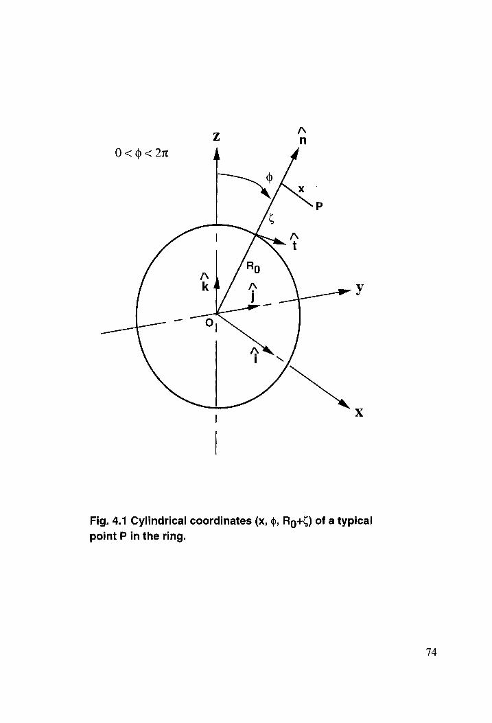
Fig. 4.1 Cylindrical coordinates (x, 0, Rg+¢) of a typical

point P in the ring.

74

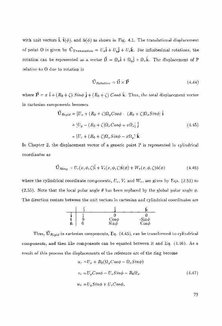
with unit vectors i, t(¢), and a(¢) as shown in Fig. 4.1. The translational displacement

of point O is given by Urranslation = Uni + Oyj + Uk. For infinitesimal rotations, the

rotation can be represented as a vector @ = Q,i+ Qyj +0,k. The displacement of P

relative to O due to rotation is

U Rotation = Q xP (4.44)

where P= ait (Ro + ©) Sind j+ (Ro + €) Cosd k. Thus, the total displacement vector

in cartesian components becomes

Urigia = (Ur + (Ro + C)QyCosd — (Ro + C)Q2 Sind] i

+ [Uy — (Ro + €C)2,Cosd + £2,] j (4.45)

a

+ [U, + (Ro + 0C)0,Sind — cQy] k

In Chapter 2, the displacement vector of a generic point P is represented in cylindrical

coordinates as

URring = U,(2, dg, ¢)i + V,(2, d, C)t(¢) + W,(2, Q, ¢)n(¢) (4.46)

where the cylindrical coordinate components, U,, V, and W,, are given by Eqs. (2.53) to

(2.55). Note that the local polar angle @ has been replaced by the global polar angle ¢.

The direction cosines between the unit vectors in cartesian and cylindrical coordinates are

n

| i j k J 1 0 0 t 0 Cosd -Sing n 0 Sing Cos

Thus, U Rigid in cartesian components, Eq. (4.45), can be transformed to cylindrical

components, and then like components can be equated between it and Eq. (4.46). As a

result of this process the displacements of the reference arc of the ring become

up =U, + Ro(Q,Cosd — 2,Sing)

vy =U,Cosd — U,Sing — RoQe (4.47)

w, =U,Singd + U,Cosé,

75

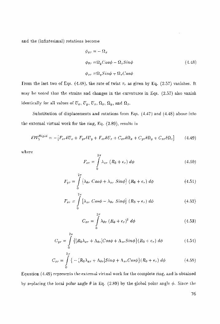
and the (infintesimal) rotations become

Par = — Qy

ber =Q,Cosd — 2,Sind (4.48)

Ger =D, Sing + 0,Cos@

From the last two of Eqs. (4.48), the rate of twist 7, as given by Eq. (2.57) vanishes. It

may be noted that the strains and changes in the curvatures in Eqs. (2.57) also vanish

identically for all values of Uz, Uy, Uz, Q2, Qy, and Nz.

Substitution of displacements and rotations from Eqs. (4.47) and (4.48) above into

the external virtual work for the ring, Eq. (2.89), results in

SWHEHE = —[ Fe 6U ey + Fyr6Uy + Fer 6Uz + Cor6Qe + Cyr6Qy + Crr622] (4.49)

where 27

Fup = / New (Ro + €p) dob (4.50) 0

27

Fyr = / [Aer ‘Cosh + Az Sing] (Ro + e,) dd (4.51)

0

20

Fi, = / [Aer Cosh — Aor Sind] (Ro + er) dd (4.52)

0

27

Cer = / Nar (Ro + er)” db (4.53) 0

27

Cyr = / {[RoAxr + Ag,|Cosd + Az, Singd}(Ro +e,) dd (4.54)

0

27

Cx = / { — [Roden + Aor]Sind + AzrCos}(Ro + er) do (4.55) 0

Equation (4.49) represents the external virtual work for the complete ring, and is obtained

by replacing the local polar angle @ in Eq. (2.89) by the global polar angle ¢. Since the

76

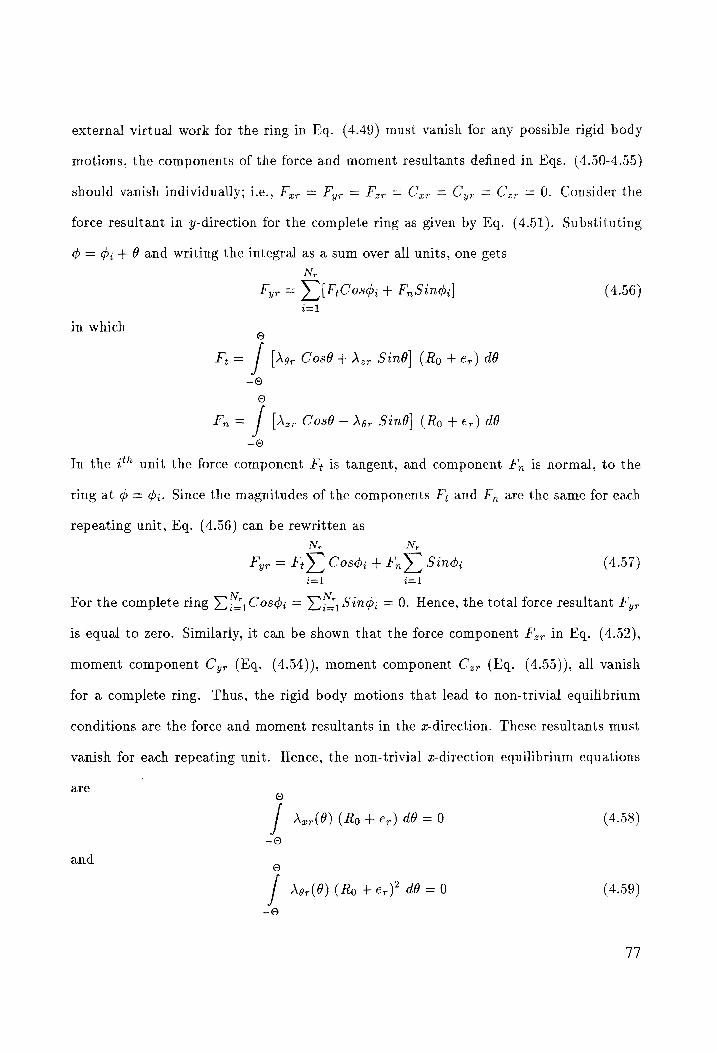
external virtual work for the ring in Eq. (4.49) must vanish for any possible rigid body

motions, the components of the force and moment resultants defined in Eqs. (4.50-4.55)

should vanish individually; i.e., Ppp = Fyr = Pip = Cor = Cyr = Cop = 0. Consider the

force resultant in y-direction for the complete ring as given by Eq. (4.51). Substituting

o = $;+ 86 and writing the integral as a sum over all units, one gets

Ny

Fyr =) [FiCosd; + FnSingi| (4.56) i=l

in which 6

Fi= / [Aor Cos + Xx Sind] (Ro + e-) dé

-0 e

fF, = / [Azr Cos@ — Aor Sin6| (Ro + €,) dé

-©

In the i** unit the force component F; is tangent, and component F,, is normal, to the

ring at @ = ¢;. Since the magnitudes of the components F; and F,, are the same for each

repeating unit, Eq. (4.56) can be rewritten as

Ny Ny

Fyr = F:S~ Cos; + Fn) Sind; (4.57) t= 1 i=l

For the complete ring a Cosd; = St, Sind; = 0. Hence, the total force resultant Fy,

is equal to zero. Similarly, it can be shown that the force component F’,, in Eq. (4.52),

moment component Cy, (Eq. (4.54)), moment component C,, (Eq. (4.55)), all vanish

for a complete ring. Thus, the rigid body motions that lead to non-trivial equilibrium

conditions are the force and moment resultants in the z-direction. These resultants must

vanish for each repeating unit. Hence, the non-trivial z-direction equilibrium equations

are ©

/ Ner(O) (Ro + er) dd =0 (4.58)

-9

and ©

/ Nor(O) (Ro + er)” dd =0 (4.59)

-O

77

4.4.22 RIGID BODY EQUILIBRIUM FOR STRINGER

For the stringer the rigid body motions are spatially uniform x-direction and z

direction displacements. (A rigid body rotation of the stringer in the z-z plane is not

considered since this motion would violate longitudinal periodicity of the repeating units.)

Vanishing of the external virtual work for an arbitrary rigid body displacement of the

stringer in the axial direction leads to the x-direction equilibrium equation

I

/ Azs(v) dx = 0 (4.60)

1

Similarly, the equilibrium equation for a rigid body displacement of the stringer in the

z-direction is

/ Azs(z) dx = 0 (4.61)

—I

4.4.3 TERMS OMITTED

Equilibrium Eqs. (4.58), (4.60) and (4.61) imply that coefficients

Arr = 0 Axs20 = 0 Azs20 = O (4.62)

in the Fourier Series for the interacting loads, and these conditions have been taken into

account in Eqs. (4.33), (4.29), and (4.30). The sine series for Ag, given in Eq. (4.34)

satisfies the equilibrium condition given in Eq. (4.59).

Consider the variational form of the constraints, Eqs. (2.90) and (2.91), for the

spatially uniform components of the virtual interacting line loads. These equations are

N t t

200 — 5 P2200 + d_{u20n - 3 %220n) — (Us20 + €5¢6320)| 6Ars20 = O (4.63)

N

> W10n — w.20| 6A2520 = 0 (4.64)

n=0

78

M t t .

200 — 5 P2200 + s (tomo — 5 Pe2mo) — (Uro + eroro)| 6Azro = 0 (4.65) mal

Since these equations are satisfied on the basis that 6Azs09 = 0, dAzs209 = O and

6Arro = O, consistent with Eq. (4.62), the bracketed terms in Eqs. (4.63) to (4.65)

do not necessarily vanish. The implication that these bracketed terms in Eqs. (4.63) to

(4.65) do not vanish is that displacement continuity conditions are not satisfied pointwise.

Pointwise continuity can be achieved by taking each Fourier coefficient appearing in the

bracketed terms of Eqs. (4.63) to (4.65) to be individually zero. Fourier Series given in

Eqs. (4.1), (4.4), (4.11), (4.13), (4.17), and (4.21) reflect this choice. Moreover, Fourier

coefficients u99, Us20, and u,yo represent rigid body displacement in the axial direction

for the shell, stringer, and ring, respectively, and setting them to zero can be justified

on the basis that rigid body displacement does not contribute to the deformation of the

structural elements. Since Fourier coefficient ws29 represents rigid body displacement of

the stringer in the z-direction, it would seem that it should be set to zero as well. However,

to maintain continuity between the stringer and the shell in the zdirection, the condition

N > Widn — W320 = O (4.66) n=0

is imposed to determine w,29 after obtaining the solution for the displacement components

that deform the shell; i.e., Fourier coefficients wio,, n = 1,...,N, are taken to be non-zero

independent degrees of freedom since the stringer coefficient ws29 is not a part of the

solution vector.

Finally, consider the constraint equation associated with éAg,o, the spatially uniform

component of the interacting moment intensity, which is omitted in the series given by

Eq. (4.36). Derived from Eq. (2.91), this constraint equation is

M

| Ss" Am Wem0 + boro|bAsro = 0 (4.67) mal

79

The constant component of the twist, 9,9, 1s equated to zero from the considerations

associated with Eq. (4.65). Consequently, a non-zero value of the uniform component of

the interacting moment intensity, Ag,o # 0, would not contribute to the equilibrium of the

ring, since Agro and ¢g,0 are conjugate variables in the external work for the ring (refer to

Eq. (2.89)). Since ¢g-9 = 0, it is necessary that Ag;o = 0 to achieve consistent conditions

for the torsional and out-of-plane bending equilibrium of the ring. With 6Ag,o = 0 in Eq.

(4.67), the bracketed term does not necessarily vanish, and as a result pointwise rotational

continuity betwen the shell and the ring is not assured. Pointwise rotational continuity is

achieved if the coefficients womo = 0, m = 1,..., M, as is done in the Fourier Series for the

normal displacement of the shell given by Eq. (4.3).

4.5 DISCRETE EQUATIONS AND THEIR SOLUTION

The Ritz method is used to obtain the system of discrete equations. The principle

of virtual work is applied separately to the shell, stringer, and ring. The virtual work

functionals are augmented by Lagrange multipliers to enforce kinematic constraints be-

tween the structural components of the repeating unit. Discrete equations for the linear

analyses are solved directly. For the nonlinear analysis an iterative solution procedure is

employed.

4.5.1 LINEAR ANALYSES

The approximations in Eqs. (4.1) through (4.28) for the actual and virtual displace-

ments, and Eqs. (4.29) through (4.42) for the actual and virtual interacting loads are

substituted into the virtual work functionals for each structural element, and also substi-

tuted into the variational form of displacement continuity constraints. Then integration

over the space is performed. This process results in a LOM N + 13M +14N +6 system of

equations for the transverse shear deformation model and 6MN+10M+11N+6 system

80

of equations for the classical model, governing the displacements and the interacting loads.

These governing equations are of the form

Ku 0 0 Bry Big Br3 Ushell Fa

0 Ko 0 Box 0 Bo3 Ustr 0

0 0 K 33 0 B39 0 Uring 0

BL BE oo 60 (lO OO] ) Awe (7) 0 (4.68) Bh 0 OBE OOO 0 0 \ring 0 Bi, Bho oO Oa 90 Q 0

in which submatrices K11, Ko2 and H33 are the stiffness matrices for the shell, stringer,

and ring, respectively, obtained from their respective internal virtual work statements.

The submatrices B;;,7,7 = 1,2,3, in Eq. (4.68) are determined from the external (or

augmented) virtual work terms involving the interacting loads, and the constraint Eqs.

(2.73), (2.74), (2.77), (2.78), (2.81), (2.82), (2.84) and (2.86). The vector on the right-

hand-side of Eq. (4.68) is the force vector, determined from the external virtual work

terms involving pressure. The constraint equations correspond to the last three rows of

the partitioned matrix in Eq. (4.68). The non-zero elements of the matrices K;;, B;; and

F\, for the transverse shear deformation and classical models are given in Appendices A

and B, respectively. The symbolic manipulation software Mathematica is used to derive

these submatrices. The discrete vectors of unknown variables (i.e. shell and stiffeners’

displacements, and shell-stiffener interacting loads) in Eq. (4.68) for the transverse shear

deformation model and classical model are given in the following two sub-subsections.

4.5.1.1 TRANSVERSE SHEAR DEFORMATION MODEL

The discrete displacement vector for the shell is the (1OMN +3M+3N 4 2)x1

vector

Ps ~T nT ~T VL Ushell = [tio y Uy seers iiy| (4.69)

in which subvectors are

. T io = [g0, W100, Y101, W101, 41015 +++) VION; W10Ns PO10N | (4.70)

81

tim = [etm Wi mds PeimOs Umi s U2m1s Vim» P21, Wim, WIm1,Peim1,P22m1>

Po1m1, PO2mI1y +> UMN > U2MNs VImNs V2MNy WimNs WamNs PrimN > (4.71)

t T Pr2mN POImN b62mn|

where m = 1,...,M

The (6M +1) x 1 discrete displacement vector for the stringer and (6N + 1) x 1 vector

for the ring are

Ustr = [915 Us115 %5215 Wels W521, P8511, PGs215 +++) UsIM, Us2M;

(4.72) T

WsiMs Ws2M,06s1M, $652M |

a T Uring = [wro Url, Uri, Wri; Peri ; Port 5 dzr1s veeg lr Ny UrN, Wren; ParN; horns bern | (4.73)

in which the term wo for the stringer has been omitted as discussed in reference to Eq.

(4.66). The 4M x 1 discrete interacting loads vector for the shell-stringer interface and

(5N +1) x 1 vector for the shell-ring interface are

a T Astr = [Azsi1 ; Ars21) Azsi1s Azs21s wey Ars1M > Ars2M> AzsiM3 Azs2M| (4.74)

A T - Aring = [Azro, Agrt ; Nori; Nzrls Nort ; Agrt; sees AgrN; AerN; ANzrN; Agrn; Azrn| (4.75)

4.5.1.2 CLASSICAL MODEL

The discrete displacement vector for the shell is the (6MN +2M+4+2N +42) x 1

vector

a a T jy tidy -ue, O44 | (4.76)

in which subvectors are

R T tio = [G0, Wr00, V101; W101) ++ VION, WioN | (4.77)

tm = [w1mo, Wim0s Uim1s U2m1) Vim1, V2m1, W1m1; W2m1,++-) VimN, V2mN;

(4.78) VimN;V2mN;,WVimN; WomN|

82

where m = 1,...,M

The (4M + 1) x 1 discrete displacement vector for the stringer and (4N + 1) x 1 vector

for the ring are

. T Geer = [G1,to11, U521, Ws11, W215 ++, Us1Ms Us2M, Ws1M >» W52M | (4.79)

a T Uring = [wro, Urls Url, Wr, Perl, +) UrNy UrN, WrN; bern | (4.80)

The 4M x 1 discrete interacting loads vector for the shell-stringer interface and (5N+1)x1

vector for the shell-ring interface are the same as for the shear deformation model and are

given by Eqs. (4.74) and (4.75).

The stiffness submatrices Ky1, Ko. and K33 in Eq. (4.68) are symmetric. From

Appendices A and B, it may be noted that the elements of the shell stiffness matrix Ay

are sparsely populated because of the orthogonality of the Fourier Series. The structure

of Ky, is block diagonal; i.e., nonzero elements occur for index p of the test function equal

to index m of the trial function, and index gq of the test function equal to index n of the

trial function. See Fig. 4.2. Furthermore, there is a decoupling of the elements obtained

from the displacement and rotation approximations using single and double Fourier series.

This special nature of the shell stiffness matrix AK 1, makes it possible to invert the matrix

in blocks (i.e., as blocks of 2 x 2 or 6 x 6 submatrices, etc.) instead of inverting the

matrix as a whole (i.e., as (6MN+2M+2N+2)x(6MN+2M +2N +2) matrix). This

results in considerable saving of the CPU time. As an example consider the linear analysis

with Fourier Series approximations truncated at 8 harmonics in z- and @-directions, i.e.,

M=WN =8. This results in 418 x 418 Ky, matrix for the classical structural model. It

takes 20 seconds of CPU time on IBM 3090 machine when the shell stiffness matrix Ay

is inverted in blocks compared to 71 seconds of CPU time on the same computer when

the matrix is inverted as a whole.

83

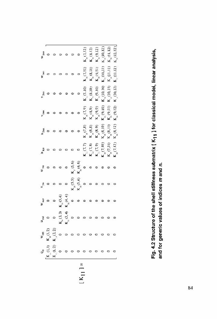
‘U puke

LW SBDIPU!

Jo SaNnjeA

d149UEH JO}

puke ‘sisAjeue

seaul| ‘japow

jeoissejo 104

[ | ly

] xiwewqns sseuyns

[Jays ou}

Jo ainjonals

zp “Bly

27D M

(ZEID MX ODM

(ZI) MH CZ) HM

CZ 0

0 0

0 0

0 7

cal

cell cay

ll eel

cay tl

ool (ID

YM GUID

WY CAton

W Cie)

XM Ais)

XH AO

yw 0

0 0

0 0

0 cel

cell

yl {ll

eH

cll

(zt0D 4

GOD

HX OOD’

MH (Core)

% (018)

MN (Orn)

0 0

0 0

0 0

oll

{Vu ca

ell

eal ell

(716) 4

CI6) YM

Ol)

XY 66)

XM 69

YN 60H

0 0

0 0

0 0

‘ tl

‘ II

‘ VW

‘ Ul

‘ Il

‘ Il

i3) 4%

t's)’ a

(Cors)"w (3)"yx

(9"y

"Hy 0

0 0

0 0

0 ‘

li ‘

it ‘

i ‘

U ‘

tl ‘

tl

(714) MY

Git) MY

OVD xX

6H"

@&WO"X CD'y

0 0

0 0

0 0

Il cll

call =

[ a

] 0

0 0

0 0

0 (99)

3M (9'9)

0 0

0 0

0 0

0 0

0 0

(9s) ¥

(Ss)

0 0

0 0

0 0

0 0

0 0

0 0

(phy

&‘O'y 0

0

0 0

0 0

0 0

0 0

(ro aM

(€) ¥

0 0

0 0

0 0

0 0

0 0

0 0

(%2' a

(D'x

| 0

0 0

0 0

0 0

0 0

0 @D x aD or,

wUz 4

UT A

wUz 4

uy wuz

ww uO

yy vol,

OU A

Oty 001 4,

oH

84

Equation (4.68) is first solved for the displacements in terms of interacting loads,

then this solution is substituted into the constraint equations to determine the interacting

loads. Thus, the total solution is obtained. An LU decomposition procedure is used to

invert the blocks in the stiffness submatrices, 41, Ko. and K33.

4.5.2 NONLINEAR ANALYSIS

As stated earlier, the nonlinear analysis is performed for the repeating unit with

symmetrical section stiffeners only. On the basis of symmetry of the repeating unit about

z- and 6-axes, the displacements and interacting loads approximations are modified for the

nonlinear analysis. In Eqs. (4.1) through (4.3) for shell displacements, in Eqs. (4.11) and

(4.12) for stringer displacements, in Eqs. (4.17) and (4.20) to (4.22) for ring displacements,

in Eqs. (4.29) and (4.30) for the shell-stringer interacting loads, and in Eqs. (4.33), (4.36)

and (4.37) for the shell-ring interacting loads, the coefficients tamn, Vomn, Womn, Us2m>

Wsims Urns Pern, Porns Perns Axs2ms Azsims Axrn, Agrn, and Azrn, all are set to zero where

m=1,2,...,.M and n=1,2,...,N. Note that the corresponding coefficients in the virtual

displacements and interacting load approximations (Eqs. (4.6-4.8), (4.14), (4.15), (4.23),

(4.26-4.28), (4.31), (4.32), (4.38), (4.41), and (4.42)) for the shell and stiffeners are also

set to zero. These modified approximations for the displacements are substituted into the

actual and the incremental virtual work functionals derived for each structural element

in Section 3.5. The incremental displacements have the same functional forms as the

actual displacements, with the amplitudes denoted by the prefix A. The integration over

space is performed after substitution for the Lagrange multipliers, or interacting loads,

and after substitution for each virtual displacement. This process results in a 3M N +

6M +6N +6 system of equations governing the increment in displacements (indicated

by a A preceding the displacement subvector symbol) and the Lagrange multipliers. The

85

governing equations are of the form

Atishell Resnett(Ushell} a)

Atstr ~Rstr(tser)

Ai, | _ —Rp( tip) [Cc] ken > 0 (4.81)

Ar 0

Q 0

where the system matrix [C] is given by

Ky1 (shen) — pL(snet) 0 0 By Bi. Bis 0 K29(tstr) 0 By 0 Ba

_ 0 () K33(t,) 0 B39 0

[e] = Bi, BE 0 0 0 0 (4.82) Bi, 0 Bi, 0 oO 0 BH, Be, 0 0 oO 0

Submatrices Ay,, Ko and K33 are the tangent stiffness matrices for the shell, stringer,

and ring, respectively, that are functions of the displacements. These matrices are ob-

tained from their respective incremental internal virtual work statements. The matrix L

results from the incremental external virtual work functional for the hydrostatic pressure,

Eq. (3.53), and is a function of displacements as well. The submatrices B;;,2,7 = 1,2,3,

in Eq. (4.82) are determined from the external virtual work terms involving the Lagrange

multipliers, and the constraint Eqs. (2.73), (2.74), (2.77) and (2.81). These B;; submatri-

ces are not functions of the displacements. The vector on the right-hand-side of Eq. (4.81)

is the residual force vector. The subvectors of Rsnrei, Rsir, and R, of the residual force

vector are obtained from the internal and external virtual work (due to internal pressure,

Eq. (3.30)) statements of the respective structural element. The constraint equations

correspond to the last three rows of the partitioned matrix in Eq. (4.82). The elements of

submatrices K;; and ZL are given in Appendix C, and the elements of subvectors Renew,

Rr and R, are given in Appendix D. The elements of submatrices B;; are obtained from

those given in Appendix B for the classical model by neglecting the elements corresponding

to the coefficients set to zero based on the symmetry of the stiffeners.

86

The discrete displacement vector for the shell in Eq. (4.81) is the (3MN + 2M +

2N + 2) x 1 vector

n n A a T Ushell — [ag al, sees aay] (4.83)

in which the subvectors are

. T uo =[¢0,Wo0, 01; Wo1;-+-s VON; Won |

, (4.84) tm = [Umo, Wm0,Um1,Um1,Wm1;+-+)UmNsUmN; WmN|

where m = 1,...,M. In Eq. (4.81) the (2M +1) x 1 discrete displacement vector for the

stringer and (2N + 1) x 1 vector for the ring are

n T Ustr =[1,Ust, Ws1, +++) UM Wsm|

(4.85) a T Ur = [wro, Url, Wrl, ++) UrN; Wrn|

The discrete vectors of the Lagrange multipliers are

° T Astr = [Acs1 »Azs1 pee ArsM; AzsM|

(4.86) T

dp = [Azro, Nérts Azrly very Norn; AzrN]

The iterative method of solution is based on Eq. (4.81). At a fixed value of the

pressure p, a sequence of displacements is defined by adding an increment to the previous

member of the sequence to determine the next member in the sequence. For a good

initial displacement estimate, the sequence converges to the displacement solution of the

nonlinear problem. The initial estimate used here is the converged solution at the last

pressure load step. The update procedure to determine the increment is based on the

modified Newton method. In the modified Newton method the matrices Ky,, Ko. and

K33, and L in Eq. (4.82) are only computed for the initial displacement in the sequence,

and are not updated for each new member in the sequence. As shown in Eqs. (4.81) and

(4.82) the constraints are applied to the increments in the displacements. If the initial

estimate of the displacement satisfies these constraint equations and the increments satisfy

87

these same equations, then the final displacement in the sequence will satisfy these same

equations.

The convergence of the solution at a fixed load step implies that the equilibrium

of the repeating unit is attained at that load step. Thus, at the converged solution the

residual defined by 6Wezt — 6Wint = 647 R, and the change in displacements A@ should be

sufficiently small. A reasonable criterion for convergence test can be to minimize Ad! R,

where the virtual displacements are replaced by the (admissible) incremental displacement

vector. An error function defined as Ati? R is used to check the convergence against a

preset tolerance, i.e, AG? R < TOL at the converged solution. In the present analysis,

this error function is formulated as

Aa? R = ABS|AG@,.i[Rsne — Brrdsir ~ Brody — BisQ]|

+ ABS [Aad [— Roce ~ BoXsir — BQ] (4.87)

+ ABS Aa? [—R, — B32 A,]|

The stiffness submatrices (441 — pL), Ko. and K33 in Eq. (4.82) are symmetric.

From Appendix C, it may be noted that the elements of the stiffness matrix for the shell,

Ky, are densely populated inspite of orthogonality of the series. Furthermore, in the

nonlinear analysis there is a coupling of the elements obtained from the displacement

approximations using single and double Fourier Series. Thus, the shell stiffness matrix

(11 — pL) cannot be inverted in the blocks as is done in the case of linear analysis.

Instead, the matrix is now required to be inverted as a whole (i.e., as (3MN + 2M +

2N+2)x(83MN+2M+42N +2) matrix), and hence, is computationally more expensive.

Equation (4.81) is first solved for the displacements in terms of interacting loads, then this

solution is substituted into the constraint equations to determine the interacting loads.

Thus, the total solution is obtained. An LU decomposition procedure is used to invert

the stiffness submatrices.

88

4.5.3. VERIFICATION OF NUMERICAL SOLUTION

Separate FORTRAN computer programs are written for the linear and nonlinear

analyses. In each program several checks on the numerical results are coded to establish

necessary conditions for the solution accuracy. These are

1. The solution for the Fourier coefficients for the displacements and interacting

loads are substituted into the left-hand side of the Eq. (4.68) to compute the force vector.

This computed force vector is compared to the input force vector to check the accuracy

of the numerical solution to Eq. (4.68).

2. From free body diagrams of the shell, stringer, and ring, overall equilibrium

conditions are established for each. These overall] equilibrium conditions are evaluated

using the numerical solution to check if they are satisfied.

3. Pointwise equilibrium equations, or the Euler equations for the functionals, are

not necessarily satisfied by the Ritz method. However, for the stringer and ring in the

present analysis, the Ritz solution is an exact solution of the Euler equations as well.

Consequently, the Euler equations for the stiffeners are programmed and evaluated at

many points using the numerical solution to assess accuracy.

4. For the nonlinear analysis the accuracy of the numerical results at each load step

is ensured by checking the error function defined by Eq. (4.87) against a preset tolerance.

At the converged solution the left-hand and right-hand sides of Eq. (4.81) are individually

equal to zero, and this is verified by the error function given by Eq. (4.87). Furthermore,

for the converged solution at final load step, the final displacements in the sequence are

substituted into the displacement constraint equations at the shell-stiffener interface to

verify them.

All numerical results presented in the following chapters satisfy these checks on

numerical accuracy.

89

CHAPTER 5

A UNIT CELL MODEL WITH SYMMETRIC STIFFENERS

5.1 INTRODUCTION

Numerical results are obtained for a linear elastic and a geometrically nonlinear

elastic response of the unit cell model subjected to internal pressure. The stiffeners are

assumed to have symmetrical cross sections. The purpose of the linear elastic analysis is

two fold: First, the results obtained are used to validate the structural model employed in

the analysis by comparing to the results presented by Wang and Hsu!9. Second, these re-

sults for the linear elastic response are subsequently used to compare with a geometrically

nonlinear elastic response. Data used in the example are representative of the dimensions

and cabin pressure of a large transport fuselage structure.

5.2 NUMERICAL DATA

Numerical data for the example are R = 117.5 in., 2! = 20 in., 2RO = 5.8 in.,

t = 0.075 in., Ro = 113.72 in., es = 1.10 in., e, = 3.78 in., (EA), = 0.592 x 107 Ib.,

(EI), = 0.269 x 10® lb-in?., (EA), = 0.404 x 10 Ib., (EJ), = 0.142 x 108 Ib-in?., and

with the shell wall stiffness matrices given by

0.664 0.221 0 A = |0.221 0.577 O | x 10° lb/in. B= 0

0 0 0.221

262 159 4.33

D = | 159 210 4.33] 1b in.

4.33 4.33 159

This data was originally used in an example by Wang and Hsu!®. In their analysis,

Wang and Hsu neglected the contribution of bend-twist coupling terms Dyg and Dog in

90

the bending stiffness matrix of shell. This implies that the shell wall is assumed to be

specially orthotropic. The present analysis is also based on the same assumption. All the

results presented for this example are for an internal pressure p = 10 psi. The Fourier

Series are truncated at M = N = 16 (unless otherwise indicated), and this results in 966

degrees of freedom (or equations to be solved) in the structural model. Since 20 = 2.83°,

the shell in this example is shallow and the DMV shell theory should be adequate. It is

found that the numerical results using Sanders theory with the rotation about the normal

neglected and the numerical results using DMV theory were essentially the same.

5.3. VALIDATION OF STRUCTURAL MODEL

The results obtained from the linear elastic analysis are compared with those ob-

tained by Wang and Hsu!9 to validate the structural model. They presented the results for

the normal displacement and strains of shell, which are limited to linear analysis. Wang

and Hsu included the interacting loads in their analysis but did not present results for

them. The distributions of the shell’s normal displacement w in the circumferential and

axial directions are shown in Figs. 5.1 and 5.2, respectively, for the linear analysis. The

w-distributions shown for the linear analysis compare very well with those presented by

Wang and Hsu (see Fig. 5 in Ref. [19]). The distributions of the circumferential and axial

normal strains on the inner and outer surfaces of the shell from the linear analysis are

shown in Figs. 5.3 and 5.4, respectively. The values of the €,, and €gg strains compare

very well to those presented by Wang and Hsu (see Figs. 6 and 7 in Ref. [19]), except in

one respect. The exception is that the circumferential distribution of the axial strain €z,

at x = —/l (Fig. 5.4) does not exhibit a decrease in value as the stringer is approached.

Wang and Hsu’s results, however, show érz (Fig. 6 in Ref. [19]) decreasing to nearly

zero as the stringer is approached along the circumference. Several changes to the shell

displacement approximations were attempted, but any of these attempts could not give

9]

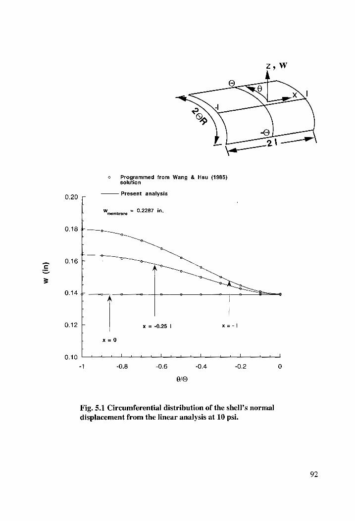
w (i

n)

QO Programmed from Wang & Hsu (1985) solution

0.20 - Present analysis

Ww = 0.2287 in. membrane

0.12 :

x = -0.25 | x=-]

x=0

I mn | 1 | | i 1 __| al Led, _| a | 1 |

-1 -0.8 -0.6 -0.4 -0.2

9/0

Fig. 5.1 Circumferential distribution of the shell’s normal

displacement from the linear analysis at 10 psi.

92

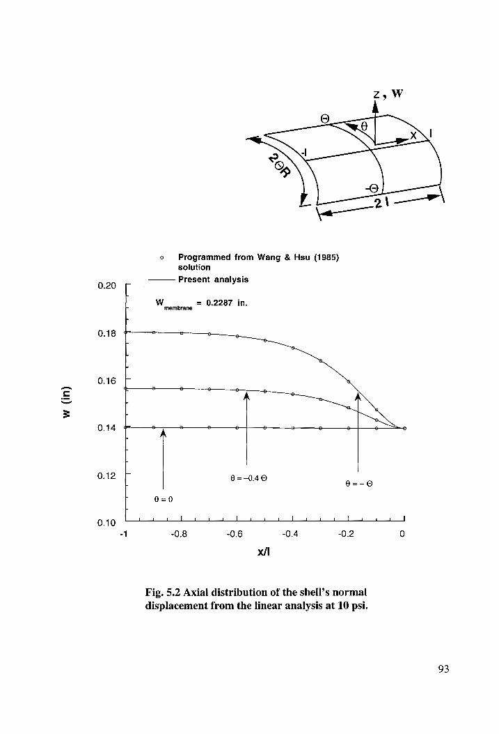
w (i

n)

0.20

0.18

0.16

0.14

0.12

0.10

t |

tT

——

o Programmed from Wang & Hsu (1985) solution

Present analysis

= 0.2287 in. membrane

6=-0.40

Deel L _| | a | J eel, unl. all — | al. j J. a a |

-0.8 -0.6 -0.4 -0.2 0

x/l

Fig. 5.2 Axial distribution of the shell’s normal

displacement from the linear analysis at 10 psi.

93

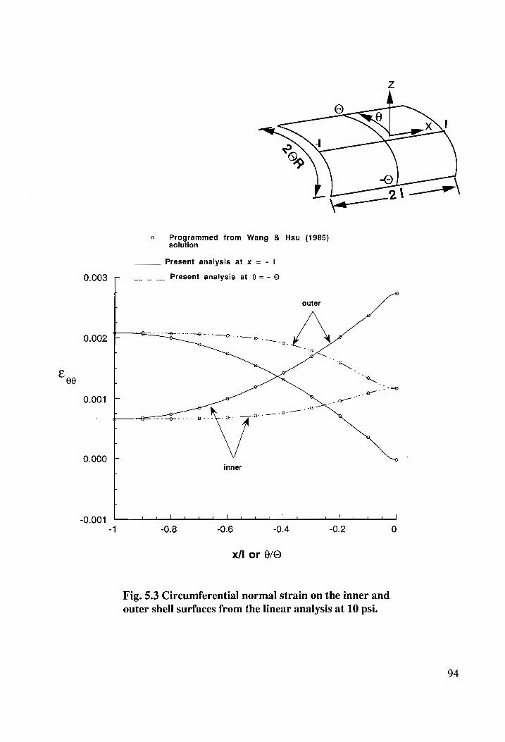
° Programmed from Wang & Hsu (1985) solution

Present analysis at x = - |

0.003 - -_-— __ Present analysis at 6=- 0

0.002 |

E 66

0.001

0.000

-0.001 _! | ! | ! ! i | ! Ld ! | ! ! j i i |

-1 -0.8 -0.6 -0.4 -0.2 0

x/l or 6/0

Fig. 5.3 Circumferential normal strain on the inner and

outer shell surfaces from the linear analysis at 10 psi.

94

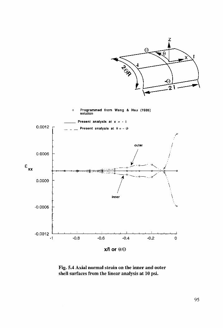
0.0012

0.0006

0.0000

-0.0006

-0.0012

2 Y \ 3

—— ——+\

fe) Programmed from Wang & Hsu (1985) solution

Present analysis at x = - |

__ Present analysis at 6 =- ©

outer /

\

| inner \

B ‘

y

L

1 | mee __| —_l. —_. l 4 ere _ _| | 1 al _] el ml. el __|

-1 -0.8 -0.6 -0.4 -0.2 0

x/I or 6/O

Fig. 5.4 Axial normal strain on the inner and outer

shell surfaces from the linear analysis at 10 psi.

95

a solution showing a decrease in the axial normal strain at the stringer. As a last resort

Wang and Hsu’s solution was programmed. However, as shown in Figs. 5.1 to 5.4, the

solution thus obtained only reconfirmed the results obtained from the current analysis,

and did not show a decrease in the axial normal strain at the stringer.

5.4 LINEAR RESPONSE VERSUS NONLINEAR RESPONSE

5.4.1 PILLOWING

Circumferential distributions of the normal displacement w for the shell are shown

in Fig. 5.1 for the linear analysis and in Fig. 5.5 for the nonlinear analysis. Axial

distributions of the normal displacement for the shell are shown in Fig. 5.2 for the linear

analysis and in Fig. 5.6 for the nonlinear analysis. For reference, the normal displacement

for the unstiffened shell, or membrane reponse, is w = 0.2287 inches for the linear analysis,

and w = 0.2290 inches for the nonlinear analysis. The presence of the stiffeners reduces

the normal displacements from these membrane values as is shown in these figures. The

pillowing effect is much more pronounced for the linear analysis (Figs. 5.1 and 5.2) than

for the nonlinear analysis (Figs. 5.5 and 5.6). The largest normal displacement occurs

midway between the stiffeners, and this value for the linear analysis is 0.1796 inches

while it is 0.1541 inches when geometric nonlinearity is included. The minimum normal

displacement occurs at the stiffener intersection, and its value is 0.1392 inches in the

linear analysis and 0.1490 inches in the nonlinear analysis. Normal displacements along

the stiffeners vary only slightly from their values at the intersection for both analyses.

Thus, including geometric nonlinearity in the analysis increases the minimum value of the

normal displacement of the shell and decreases its maximum value, which is an indication

that pillowing is reduced in the nonlinear response.

96

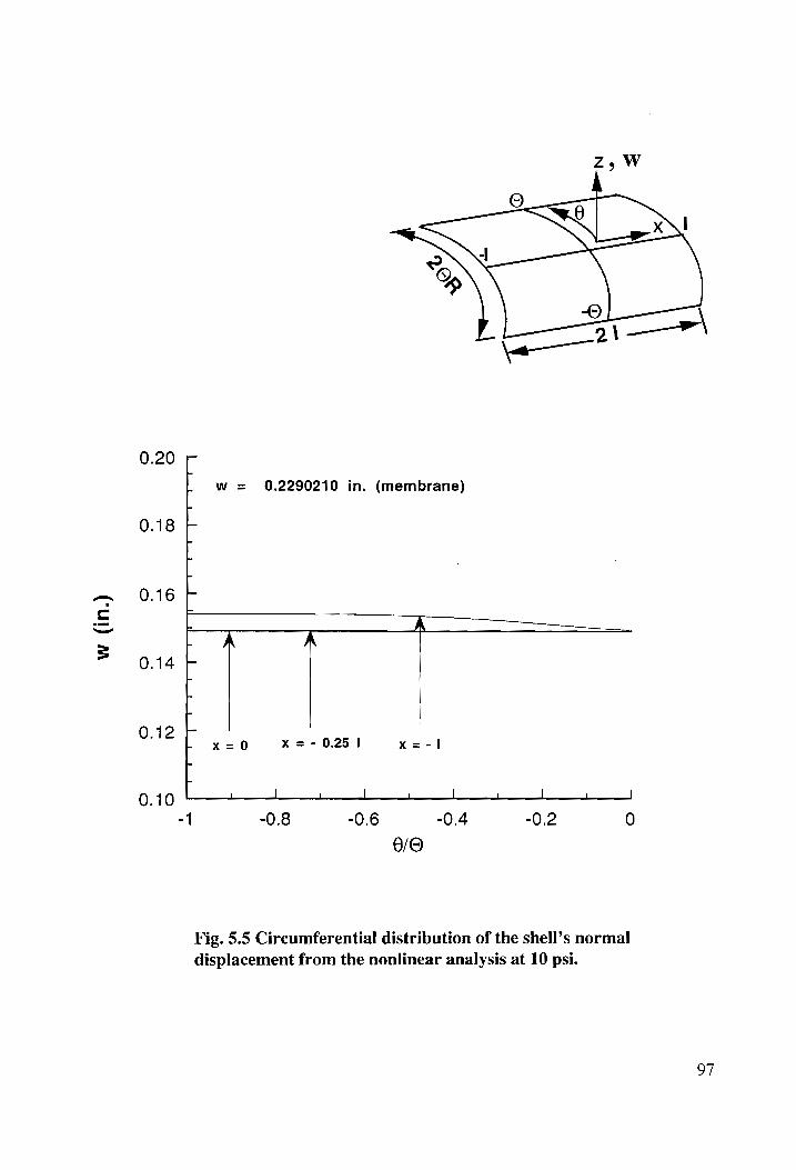
w (in.)

0.20

0.18

0.16

0.14

0.12

0.10

1

w = 0.2290210 in. (membrane)

r

i

P kK

i

i | x=0 x =- 0.25 | x=-|

P a | | | | lg | 1 | ee | |

-1 -0.8 -0.6 -0.4 -0.2 0

e/©

Fig. 5.5 Circumferential distribution of the shell’s normal

displacement from the nonlinear analysis at 10 psi.

97

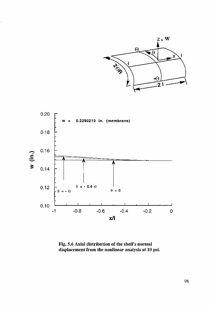
w (in.)

0.20

0.18

0.16

0.14

0.12

0.10

w = 0.2290210 in. (membrane)

t |

q t

' |

' i

a

>

>

' CT

] T

TT

YF }

1

86 =-0.40

@6=-0O0 6=0

1 _| nl, | FI | el | al, |

-1 -0.8 -0.6 -0.4 -0.2 0

Fig. 5.6 Axial distribution of the shell’s normal

displacement from the nonlinear analysis at 10 psi.

98

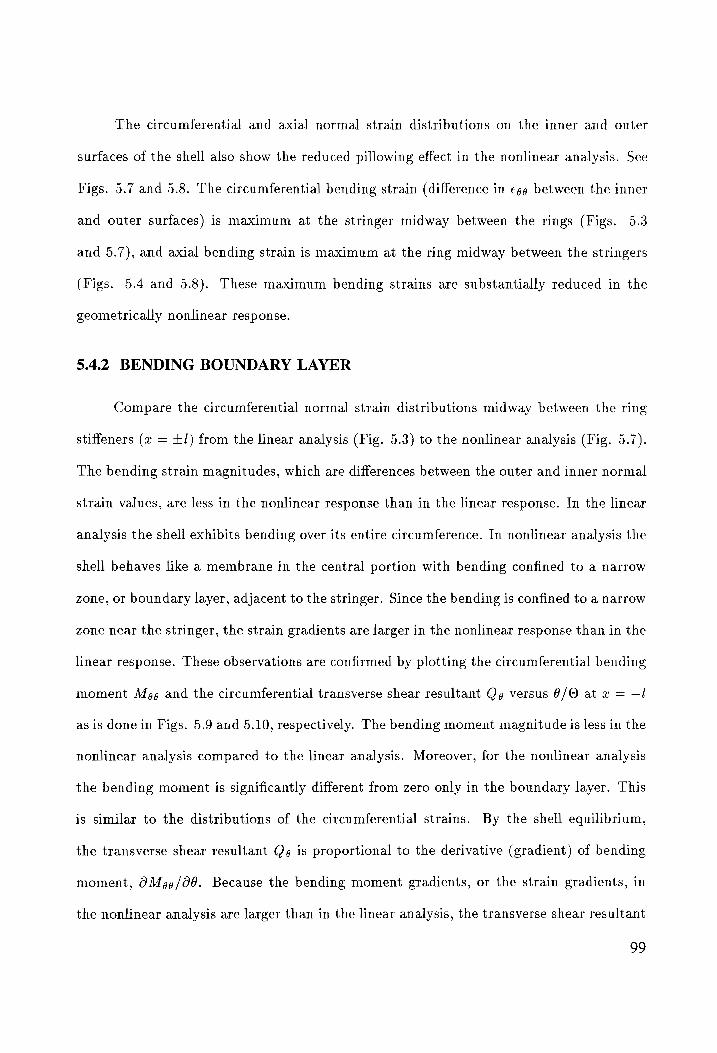
The circumferential and axial normal strain distributions on the inner and outer

surfaces of the shell also show the reduced pillowing effect in the nonlinear analysis. See

Figs. 5.7 and 5.8. The circumferential bending strain (difference in €gg between the inner

and outer surfaces) is maximum at the stringer midway between the rings (Figs. 5.3

and 5.7), and axial bending strain is maximum at the ring midway between the stringers

(Figs. 5.4 and 5.8). These maximum bending strains are substantially reduced in the

geometrically nonlinear response.

5.4.2 BENDING BOUNDARY LAYER

Compare the circumferential normal strain distributions midway between the ring

stiffeners (z = +/) from the linear analysis (Fig. 5.3) to the nonlinear analysis (Fig. 5.7).

The bending strain magnitudes, which are differences between the outer and inner normal

strain values, are less in the nonlinear response than in the linear response. In the linear

analysis the shell exhibits bending over its entire circumference. In nonlinear analysis the

shell behaves like a membrane in the central portion with bending confined to a narrow

zone, or boundary layer, adjacent to the stringer. Since the bending is confined to a narrow

zone near the stringer, the strain gradients are larger in the nonlinear response than in the

linear response. These observations are confirmed by plotting the circumferential bending

moment Mogg and the circumferential transverse shear resultant Q¢ versus 6/O at x = —1

as is done in Figs. 5.9 and 5.10, respectively. The bending moment magnitude is less in the

nonlinear analysis compared to the linear analysis. Moreover, for the nonlinear analysis

the bending moment is significantly different from zero only in the boundary layer. This

is similar to the distributions of the circumferential strains. By the shell equilibrium,

the transverse shear resultant Q¢ is proportional to the derivative (gradient) of bending

moment, 0Mge/00. Because the bending moment gradients, or the strain gradients, in

the nonlinear analysis are larger than in the linear analysis, the transverse shear resultant

99

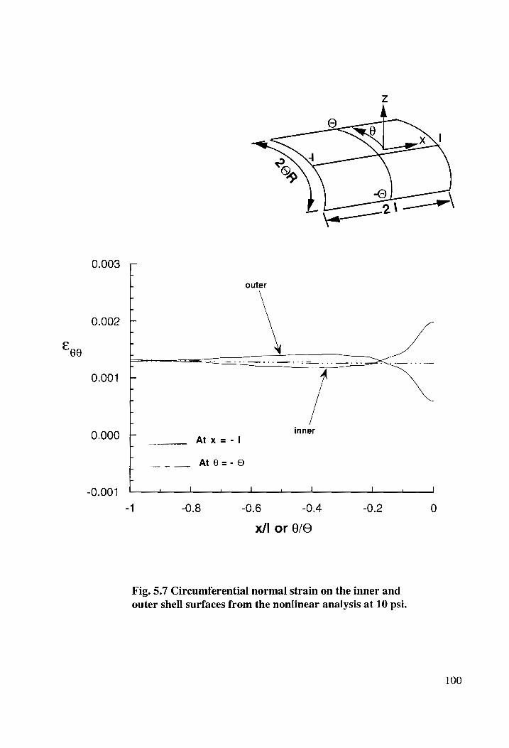
0.003

0.002

00

0.001

0.000

-0.001

outer

|

|

L atx ect inner

L ___- At O=-0O

f _ _] ! __| ! __| | __| 4 |

-1 -0.8 -0.6 -0.4 -0.2 0

x/I or 8/0

Fig. 5.7 Circumferential normal strain on the inner and

outer shell surfaces from the nonlinear analysis at 10 psi.

100

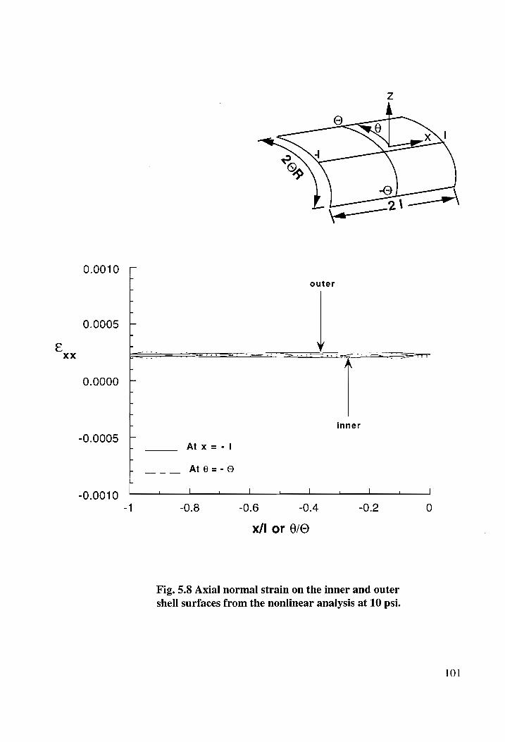
XX

0.0010

0.0005

0.0000

-0.0005

-0.0010

; outer

- SSS — = = = 2S

r inner

At x =- 1

- _ At@=-0

P l | l | l | l | l

-1 -0.8 -0.6 -0.4 -0.2

x/l or 8/0

Fig. 5.8 Axial normal strain on the inner and outer

shell surfaces from the nonlinear analysis at 10 psi.

101

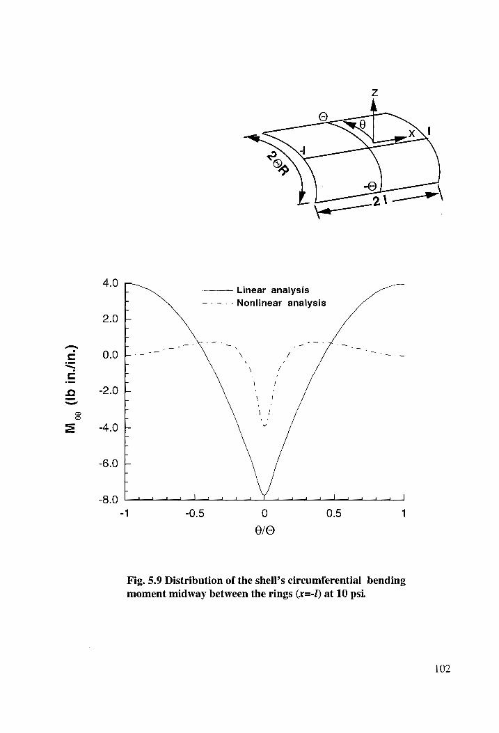
M_,

(Ib i

nJin.)

4.0

2.0

0.0

. Linear analysis

t ~--—.--Nonlinear analysis

- -

ae _ Te

LE

E r

-

i

| |

- -0.5 0 0.5 1

Fig. 5.9 Distribution of the shell’s circumferential bending

moment midway between the rings (x=-1) at 10 psi.

102

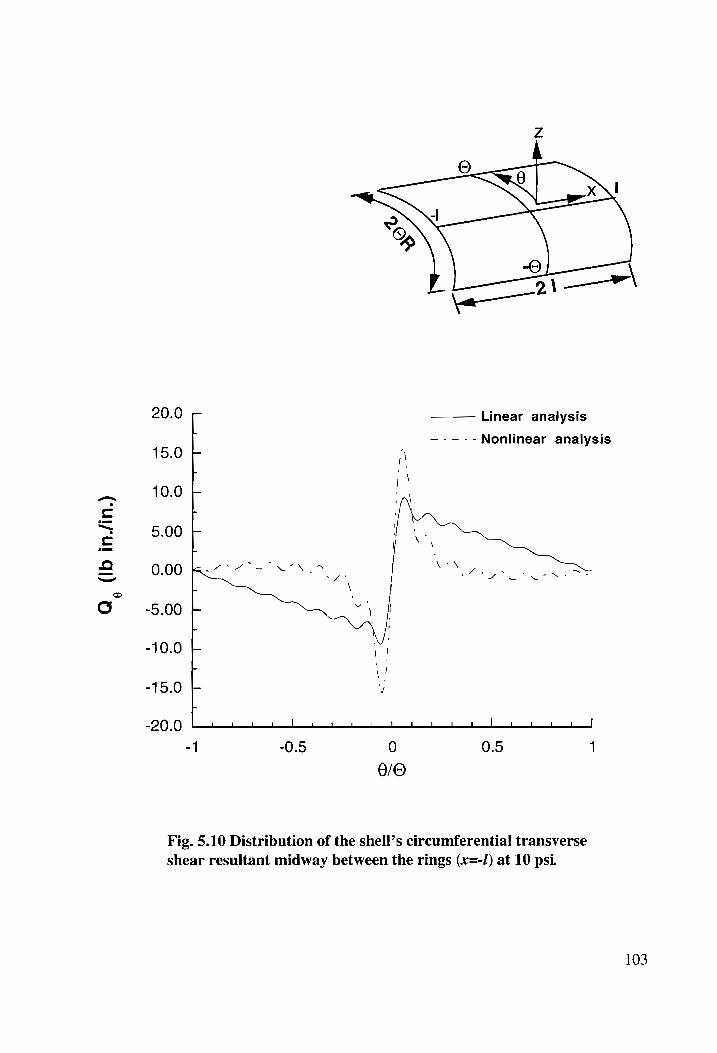
Q (Ib

in.

/in.)

8

20.0

15.0

10.0

5.00

0.00

-5.00

-10.0

-15.0

-20.0 al

Linear analysis

—--.--Nonlinear analysis

aad ad a _| pers beers eens henner _| el os

0 0.5 1

0/O

Fig. 5.10 Distribution of the shell’s circumferential transverse

shear resultant midway between the rings (x=-/) at 10 psi.

103

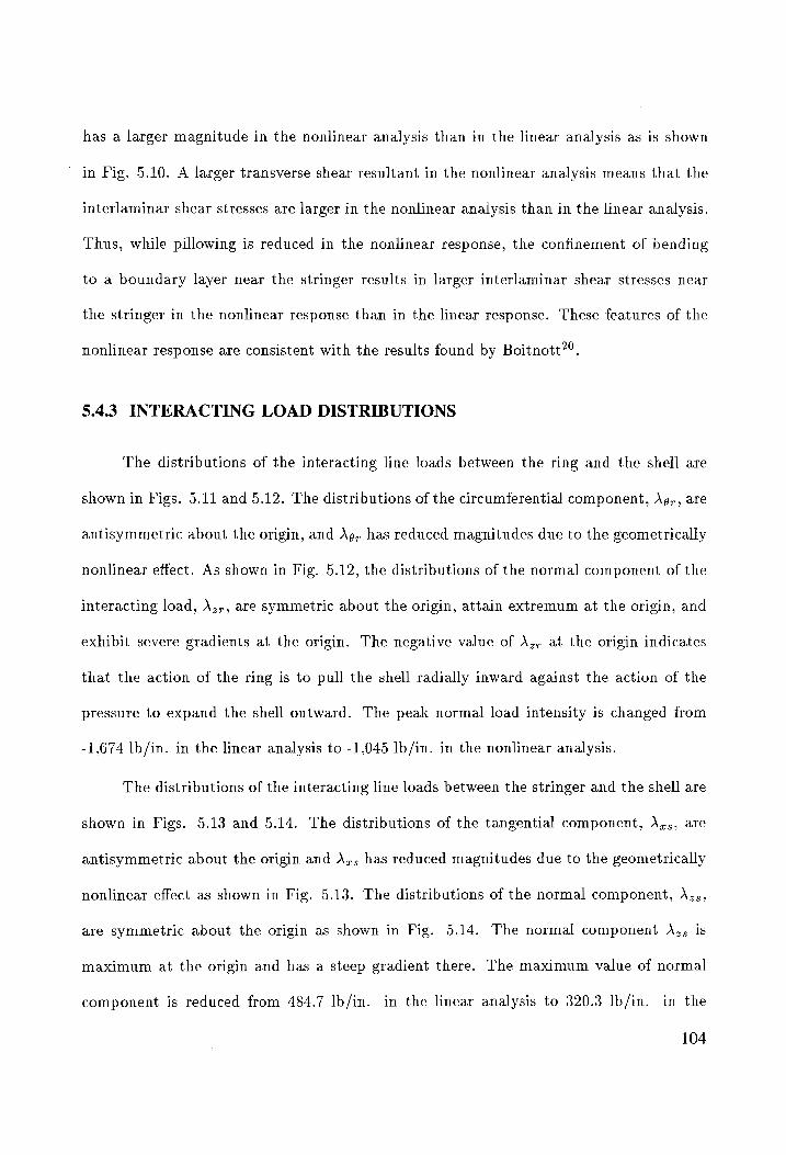
has a larger magnitude in the nonlinear analysis than in the linear analysis as is shown

in Fig. 5.10. A larger transverse shear resultant in the nonlinear analysis means that the

interlaminar shear stresses are larger in the nonlinear analysis than in the linear analysis.

Thus, while pillowing is reduced in the nonlinear response, the confinement of bending

to a boundary layer near the stringer results in larger interlaminar shear stresses near

the stringer in the nonlinear response than in the linear response. These features of the

nonlinear response are consistent with the results found by Boitnott?°.

5.4.3 INTERACTING LOAD DISTRIBUTIONS

The distributions of the interacting line loads between the ring and the shell are

shown in Figs. 5.11 and 5.12. The distributions of the circumferential component, A9,, are

antisymmetric about the origin, and Ag, has reduced magnitudes due to the geometrically

nonlinear effect. As shown in Fig. 5.12, the distributions of the normal component of the

interacting load, A,,, are symmetric about the origin, attain extremum at the origin, and

exhibit severe gradients at the origin. The negative value of A,, at the origin indicates

that the action of the ring is to pull the shell radially inward against the action of the

pressure to expand the shell outward. The peak normal load intensity is changed from

-1,674 lb/in. in the linear analysis to -1,045 lb/in. in the nonlinear analysis.

The distributions of the interacting line loads between the stringer and the shell are

shown in Figs. 5.13 and 5.14. The distributions of the tangential component, A,5, are

antisymmetric about the origin and A,, has reduced magnitudes due to the geometrically

nonlinear effect as shown in Fig. 5.13. The distributions of the normal component, Az,

are symmetric about the origin as shown in Fig. 5.14. The normal component A, is

maximum at the origin and has a steep gradient there. The maximum value of normal

component is reduced from 484.7 lb/in. in the linear analysis to 320.3 lb/in. in the

104

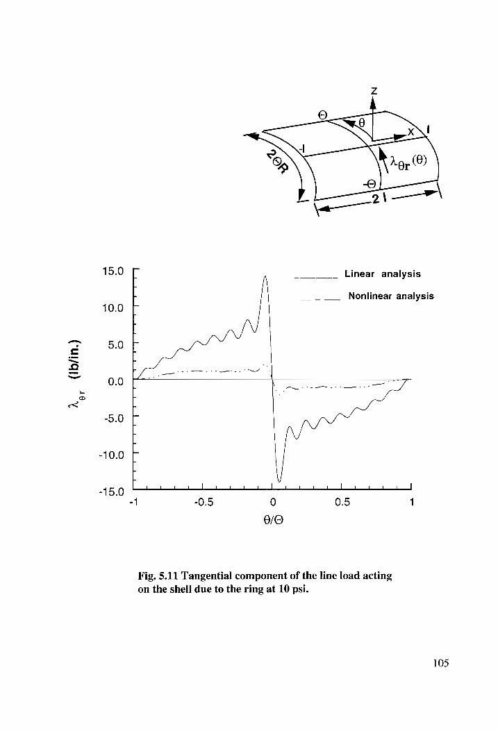
(Ib/

in.)

or

r

15.0 Linear analysis

Nonlinear analysis

10.0

5.0

T tT

] rod

i UJ

T t

1

0.0

-10.0 -15.0

' — ' © ol

Fig. 5.11 Tangential component of the line load acting

on the shell due to the ring at 10 psi.

105

(Ib/in

.) r

(Ib/in

.) r

h,

ar

-1200.0 F

r -1600.0 [

-2000.0

200.0

100.0 '

0.0

-100.0 " -200.0

400.0

0.0 -400.0 Linear analysis

800.0 i ____ Nonlinear analysis 1 -0.5 0 0.5 1

Fig. 5.12 Normal component of the line load acting

on the shell due to the ring at 10 psi.

106

(Ib/in

.) xs

XV

40.0

20.0

0.0

-20.0

-40.0

Linear analysis I”

T T

Nonlinear analysis

‘

s

Fig. 5.13 Tangential component of the line load acting

on the shell due to the stringer at 10 psi.

107

(Ib/

in.)

zs

Xr (Ib

/in.)

zs

r

75.0 r

50.0 -

25.0

0.0

-25.0 -50.0 -75.0

-100.0

-125.0 -

500.0 Linear analysis

Nonlinear analysis

400.0

300.0

200.0

100.0

0.0 K7

-100.0

-200.0 l 1 L | i. l L L | 1 1 1 i | 1 i l ul |

-1 -

Fig. 5.14 Normal component of the line load acting

on the shell due to the stringer at 10 psi.

108

nonlinear analysis. Note that the resultant of this normal component vanishes as a result

of Eq. (4.61).

5.4.4 STIFFENER ACTIONS

The distributions of the force and moment resultants in the stiffeners are shown in

Figs. 5.15 and 5.16. In the linear analysis the total axial load due to the 10 psi pressure

is 3,407.5 lbs (= pR*O), and the portion of this load carried by the stringer is 820.1 lbs,

or about 24% of the total axial load, according to the value of N,, at x = +1 shown

in Fig. 5.15. For the nonlinear analysis at 10 psi, the axial load carried by the stringer

is increased to about 861.4 lbs, or 25.2% of the total axial load. In both the linear and

nonlinear analyses, the axial force in the stringer increases slightly from its minimum value

midway between the rings to a maximum at the ring location. The bending moment in

the ring is reduced by the geometric nonlinearity at the expense of an increase in the

value of the circumferential force Ng, as shown in Fig. 5.16. In the linear analysis the

total circumferential force due to the 10 psi pressure is 23,500 lbs (= pR x 21). The

circumferential force in the ring is nearly uniform and increases from 7,242 lbs in the

linear analysis to 7,757 lbs in the nonlinear analysis. Thus, the force resultants in the

stiffeners increase due to the inclusion of geometric nonlinearity in the analysis.

5.5 SINGULARITY AT THE SHELL-STRINGER-RING JOINT

The results for the interacting normal loads \,, and A,, (Figs. 5.12 and 5.14)

suggest that they exhibit singular behavior at the stiffener intersection. It is expected

that the increased stiffness normal to the structure at the joint, or stiffener intersection,

would result in increased normal loads. However, it is likely that the singular behavior at

the joint is a mathematical artifact of modeling the contact zone between the shell and

stiffeners as a point. The argument for singular behavior is supported by plotting the

109

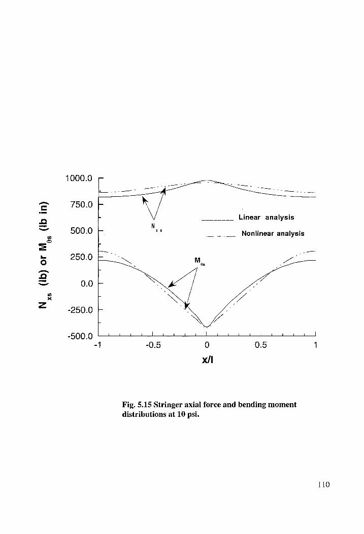
(ib)

or

M,,

(Ib

in)

xs

N

1000.0

750.0

500.0

290.0

0.0

-250.0

-500.0

a Linear analysis

N

t i ____ Nonlinear analysis L

i . ww M.. . 2

J | J |

-1 1

Fig. 5.15 Stringer axial force and bending moment

distributions at 10 psi.

110

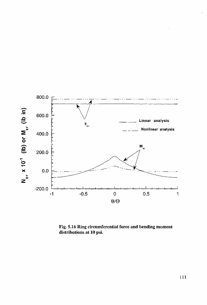
(Ib

in)

xr

(Ib)

or

M N

x10"

er

800.0

600.0

400.0

200.0

0.0

Linear analysis

or

Nonlinear analysis

—l 4 po ml | ! m __| — al

-1 -0.5 0 0.5

8/0

Fig. 5.16 Ring circumferential force and bending moment


111

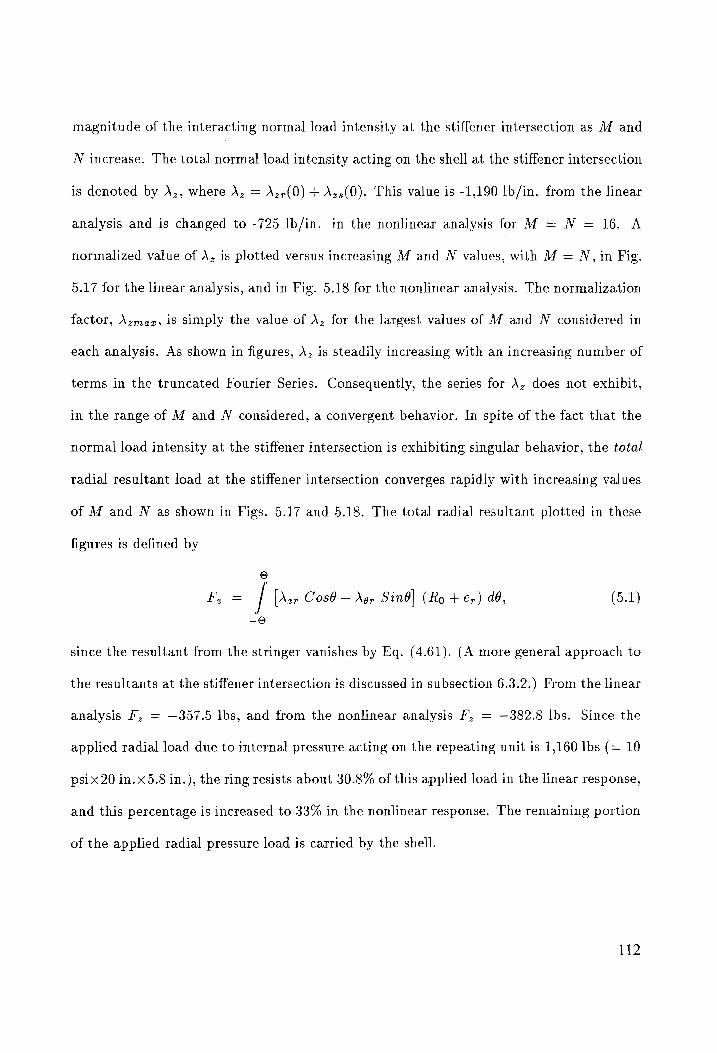
magnitude of the interacting normal load intensity at the stiffener intersection as M and

N increase. The total normal load intensity acting on the shell at the stiffener intersection

is denoted by Az, where A, = A27(0) + Azs(0). This value is -1,190 lb/in. from the linear

analysis and is changed to -725 lb/in. in the nonlinear analysis for M = N = 16. A

normalized value of A, is plotted versus increasing M and N values, with M = N, in Fig.

5.17 for the linear analysis, and in Fig. 5.18 for the nonlinear analysis. The normalization

factor, Azmaz, is simply the value of A, for the largest values of M and N considered in

each analysis. As shown in figures, A, is steadily increasing with an increasing number of

terms in the truncated Fourier Series. Consequently, the series for A, does not exhibit,

in the range of M and N considered, a convergent behavior. In spite of the fact that the

normal load intensity at the stiffener intersection is exhibiting singular behavior, the total

radial resultant load at the stiffener intersection converges rapidly with increasing values

of M and N as shown in Figs. 5.17 and 5.18. The total radial resultant plotted in these

figures is defined by

©

Fy = / [Azr Cosé — or Sind] (Ro + e,) dé, (5.1)

-©

since the resultant from the stringer vanishes by Eq. (4.61). (A more general approach to

the resultants at the stiffener intersection is discussed in subsection 6.3.2.) From the linear

analysis F, = —357.5 lbs, and from the nonlinear analysis Ff, = —382.8 lbs. Since the

applied radial load due to internal pressure acting on the repeating unit is 1,160 lbs (= 10

psix 20 in.x5.8 in.), the ring resists about 30.8% of this applied load in the linear response,

and this percentage is increased to 33% in the nonlinear response. The remaining portion

of the applied radial pressure load is carried by the shell.

112

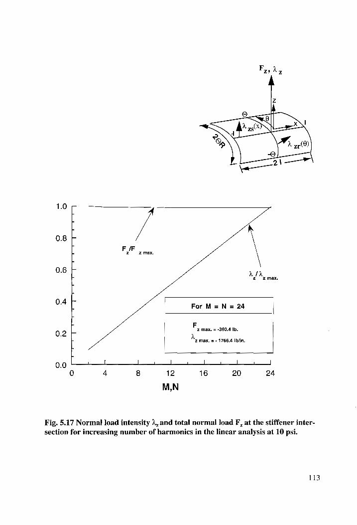
1.0

0.8

0.6

0.4

0.2

0.0

J

my,

f F /F r z

' z max.

5

r For M=N = 24

a F. max. = -360.4 Ib.

- Zz max. = - 1766.4 Ib/in.

.

i pf | i | \ | t _J

0 4 8 12 16 20 24

M,N

Fig. 5.17 Normal load intensity 1, and total normal load F, at the stiffener inter-

section for increasing number of harmonics in the linear analysis at 10 psi.

113

1.0 7

0.8 fF y Fi

0.6

0.4 i For M=N = 16

0.2 F max, = -382.8 Ib.

L z max, = - 724.8 Ib/in.

0.0 1 | \ |

0 4 8 12 16

Fig. 5.18 Normal load intensity 1, and total normal load F, at the stiffener intersection for increasing number of harmonics in the nonlinear analysis at 10 psi.

114

5.6 SUMMARY OF RESULTS

The spatial distribution of the normal displacements of the cylindrical shell are more

uniform, and the bending strains are reduced, in the geometrically nonlinear elastic anal-

ysis with respect to what is predicted by the linear elastic analysis. That is, pillowing of

the skin is reduced by the inclusion of geometric nonlinearity into the analysis. However,

in the nonlinear analysis the most severe circumferential bending is confined to a narrow

boundary layer adjacent to the stringer midway between the rings, and the interior por-

tion of the shell behaves as a membrane. In the linear analysis the bending occurs over

the entire circumference of the shell. The development of the bending boundary layer

due to the inclusion of geometric nonlinearity into the analysis causes an increase in the

circumferential transverse shear resultant in the shell adjacent to the stringer compared

to the linear analysis. Increased interlaminar shear stresses can be expected as a result of

the increased transverse shear resultant.

The distributions of the normal actions between the shell and stiffeners (A.5, Azr)

show significant magnitudes only in the vicinity of the joint, with much smaller magnitudes

away from the joint. The distributions of actions tangent to the stiffeners (Ars, Agr), on

the other hand, have small magnitudes at the joint and large magnitudes away from the

joint.

The series for the interacting normal load intensity at the stiffener intersection does

not appear to converge in both the linear analysis and in the geometrically nonlinear

analysis. The magnitude of the resultant normal load intensity at the stiffener intersection

using a trucated Fourier Series approximation is decreased by the inclusion of geometric

nonlinearity into the analysis. However, Fourier Series for the total radial resultant load

carried by the stiffeners, which is resolved at the intersection, exhibits rapid convergence.

This total radial resultant carried by the stiffeners is increased slightly by the inclusion

115

of geometric nonlinearity into the analysis. The axial force carried by the stringer due

to the closed-end pressure vessel effect is increased in the nonlinear analysis with respect

to its value in the linear analysis. Also, the circumferential force carried by the ring is

increased in the nonlinear analysis with respect to its value in the linear analysis. Thus,

the stiffeners resist an increased portion of the internal pressure load, accompanied by a

commensurate decrease in the load carried by the shell, when geometric nonlinearity is

included into the analysis.

116

CHAPTER 6

A UNIT CELL MODEL WITH AN ASYMMETRIC RING

6.1 INTRODUCTION

Numerical results are obtained for the linear elastic response of a unit cell model

with a symmetrical section stringer and an asymmetrical open section ring. The effects of

transverse shear deformations and warping deformation of the ring’s cross section on the

response are studied. Data used in the example are representative of the crown panel of

a large transport fuselage structure.

6.2 NUMERICAL DATA

Numerical data for this second example are again representative of a large transport

fuselage structure. The shell radius R = 122.0 in., frame spacing 2/ = 22 in., and stringer

spacing 2RO = 15.0 in. The shell wall is a 13-ply [+45, 90,0, +60, 90, +60, 0,90, +45],

laminate of graphite-epoxy AS4/938 tow prepreg with total thickness of 0.0962 in. The

ply thickness is 0.0074 in., and the lamina material properties are assumed to be Fy =

19.21 x 10°lb/in.?, Ey = 1.36 x 10°lb/in.?, Gig = Gig = Go3 = 0.72 x 10°%lb/in.”, and

42 = 0.32. For the transverse shear deformation model, the shell wall stiffness sub-

matrix of Eq. (2.31) is computed using these ply data and the expressions for the stiffness

elements given by Eqs. (2.32). The numerical results are

10.5774 0.2619 0 A = | 0.2619 0.9766 0 x 10° Ib/in.

| 0 0 0.2889

| 3.893 0 0.1847 0.1847 0 —5.043 —0.2213 0.2213} 1b

| 0 —0.443 —1.1351 1.1351 117

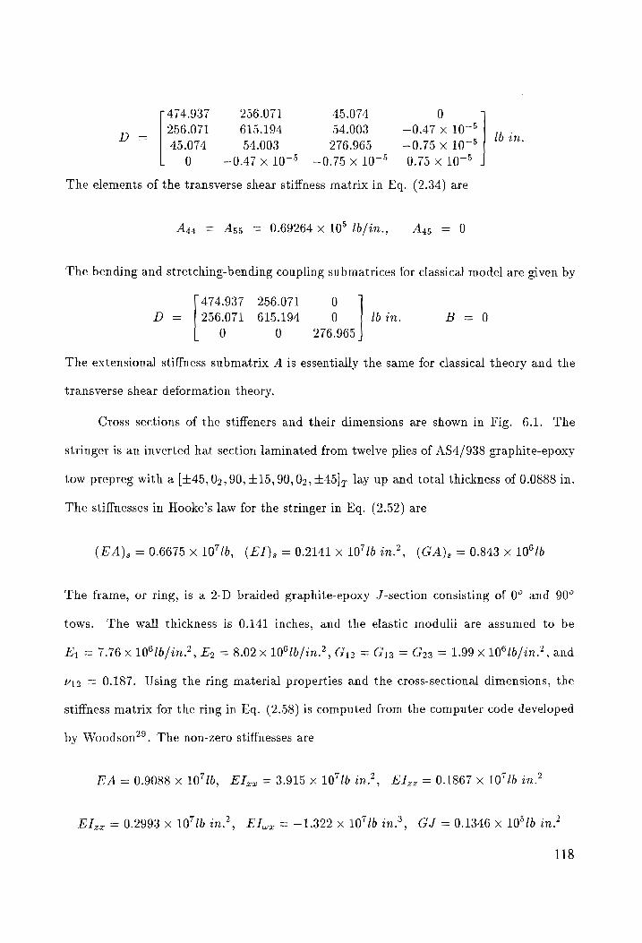
474.937 256.071 45.074 0

p —. | 256.071 615.194 54.003 —0.47 x 107° Ib in ~ | 45.074 54.003 276.965 —0.75 x 107° ~

0 —0.47x 107° -0.75x 107° 0.75 x 107°

The elements of the transverse shear stiffness matrix in Eq. (2.34) are

Ags = Ass = 0.69264 10° Ib/in., Ags = 0

The bending and stretching-bending coupling submatrices for classical model are given by

474.937 256.071 0

D = | 256.071 615.194 0 lb in. B= 0

0 0 276.965

The extensional stiffness submatrix A is essentially the same for classical theory and the

transverse shear deformation theory.

Cross sections of the stiffeners and their dimensions are shown in Fig. 6.1. The

stringer is an inverted hat section laminated from twelve plies of AS4/938 graphite-epoxy

tow prepreg with a [+45, 02, 90,+15, 90, 0.,+45], lay up and total thickness of 0.0888 in.

The stiffnesses in Hooke’s law for the stringer in Eq. (2.52) are

(EA), = 0.6675 x 10°lb, (EI), = 0.2141 x 107lb in.?, (GA), = 0.843 x 10%Ib

The frame, or ring, is a 2-D braided graphite-epoxy J-section consisting of 0° and 90°

tows. The wall thickness is 0.141 inches, and the elastic modulii are assumed to be

FE, = 7.76 x 10°lb/in.?, Ez = 8.02 x 10°lb/in.?, Gig = Gi3 = Go3 = 1.99 x 10°/b/in.’, and

vyq = 0.187. Using the ring material properties and the cross-sectional dimensions, the

stiffness matrix for the ring in Eq. (2.58) is computed from the computer code developed

by Woodson??. The non-zero stiffnesses are

EA = 0.9088 x 10°lb, EIpg = 3.915 x 107Ib in.*, El,, = 0.1867 x 10°lb in.”

Elen = 0.2993 X 1071b in.?, Ele = —1.322 x 10%b ine, GJ = 0.1346 x 10°lb in,

118

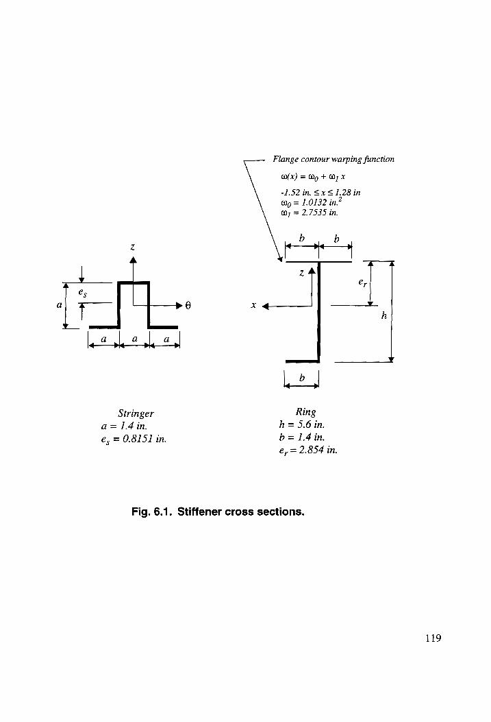
Flange contour warping function

Ox) = Wg + @; x

-1.52 in. SxS 1.28 in Wp = 1.0132 in.”

7 = 2.7535 in.

? ta 2

|

| a a a

| —________¥

Ley

Stringer Ring

= 1.4 in, h = 5.6 in.

é€, = 0.8151 in. b = 1.4 in.

€, = 2.854 in.

Fig. 6.1. Stiffener cross sections.

119

EL... = 1.705 x 101 in.4, EI, = —0.1865 x 10°/b in.®

GAgop = GAzg = 0.2396 x 107 Ib

All the results presented are for an internal pressure p = 10 psi, and the Fourier Series

are truncated at twenty-four terms in the z- and 6-directions (MM = N = 24). Based on

M = N = 24, the transverse shear deformation model consists of a total of 6414 degress

of freedom, and classical model consists of 3966 degress of freedom.

6.3 INFLUENCE OF AN ASYMMETRICAL SECTION RING

6.3.1 INTERACTING LOAD DISTRIBUTIONS

The distributions of the interacting line load intensities between the stiffeners and

the shell are shown in Figs. 6.2 through 6.8. The effects of transverse shear deformations

and of warping deformation of the ring’s cross section due to torsion on the magnitudes

of the interacting line loads are summarized in Table 6.1. For the component A,, tangent

to the stringer (Fig. 6.2), there are only small differences in the distributions as predicted

by the four structural models. However, the peak value of the component normal to the

stringer, A,,, is reduced in the transverse shear deformation models with respect to its

peak value in the classical models (Fig. 6.3 and Table 6.1).

The distributions of axial force intensity, A,,, between the ring and shell predicted

by the classical and shear deformation models with warping are nearly the same (Fig.

6.4). However, the distributions of this force intensity predicted by the classical and shear

deformation models without warping have significant differences. Thus, this interacting

load intensity is more sensitive to the inclusion or exclusion of warping of the ring cross

section into the structural model. As shown in Fig. 6.5, the differences in the results for

circumferential force intensity, Ag,, between the ring and shell from the four models are

120

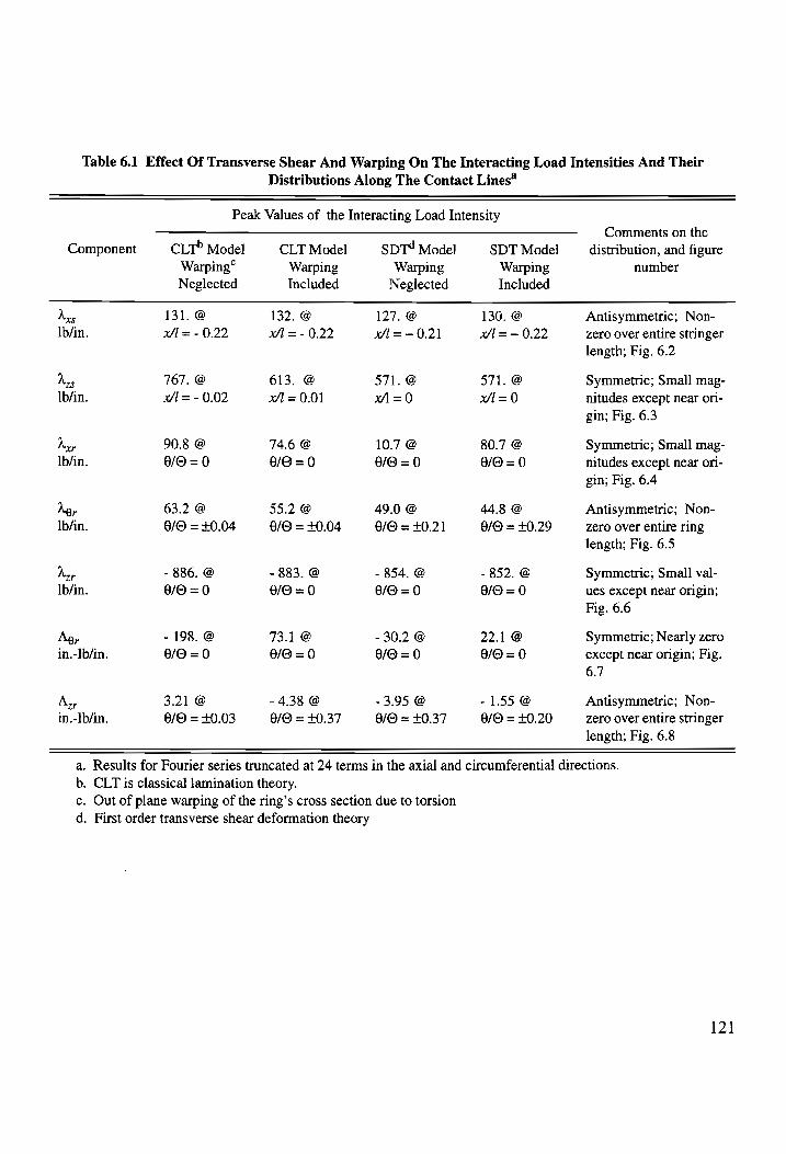
Table 6.1 Effect Of Transverse Shear And Warping On The Interacting Load Intensities And Their

Distributions Along The Contact Lines*

Peak Values of the Interacting Load Intensity Comments on the

Component CLT® Model CLT Model SDT? Model SDT Model distribution, and figure

Warping® Warping Warping Warping number Neglected Included Neglected Included

Axes 131. @ 132. @ 127. @ 130. @ Antisymmetric; Non- Ib/in. wl = - 0.22 xX = - 0.22 Wl =—-0.21 x = — 0.22 zero Over entire stringer

length; Fig. 6.2

des 767. @ 613. @ 571. @ 571. @ Symmetric; Small mag- Ib/in. xf = - 0.02 xA= 0.01 x =0 wW=0 nitudes except near ori-

gin; Fig. 6.3

Aer 90.8 @ 74.6 @ 10.7 @ 80.7 @ Symmetric; Small mag- lb/in. 6/0 = 0 6/6 = 0 6/0 = 0 6/0 = 0 nitudes except near ori-

gin; Fig. 6.4

Nor 63.2 @ 55.2 @ 49.0 @ 44.8 @ Antisymmetric; Non- Ib/in. 6/O = +0.04 0/0 = +0.04 6/0 = +0.21 6/O = +0.29 zero Over entire ring

length; Fig. 6.5

Nop - 886. @ - 883. @ - 854. @ - 852. @ Symmetric; Small val-

ib/in. 8/0 = 0 0/0 = 0 6/06 =0 8/0 = 0 ues except near origin;

Fig. 6.6

Ag, - 198. @ 73.1 @ - 30.2 @ 22.1 @ Symmetric; Nearly zero

in.-lb/in. 6/6 =0 0/0 = 0 6/06 =0 6/6 =0 except near origin; Fig.

6.7

Ay 3.21 @ - 4.38 @ - 3.95 @ - 1.55 @ Antisymmetric; Non- in.-lb/in. 6/O = +0.03 0/© = +0.37 6/© = +0.37 6/0 = +£0.20 zero over entire stringer

length; Fig. 6.8

a. Results for Fourier series truncated at 24 terms in the axial and circumferential directions.

b. CLT is classical lamination theory.

c. Out of plane warping of the ring’s cross section due to torsion

d. First order transverse shear deformation theory

121

150.0

100.0

50.0

(Ib/in)

0.0

xs

r

-50.0

-100.0

-150.0

veccceees Classical theory

Shear deform. theory

——----Classical theory w/o warping

—— - -Shear deform. theory w/o warping

Fig. 6.2 Stringer-shell tangential force intensity in axial direction

at 10 psi.

122

100.0

50.0

< _,

2

_

-50.0

-100.0 800.0

600.0

400.0 | 2 r

3 LL

2 200.0

an

-200.0 |

-400.9 Lu

0.0 k

trttestee Classical theory


—.---- Classical theory w/o warping


0.0 } “A oer

Fig. 6.3 Stringer-shell normal force intensity at 10 psi.

123

(Ib/in)

xr

r (Ib/in)

r xr

25.0 -

wo etee eee Classical theory


—.---- Classical theory w/o warping —— - - Shear deform. theory w/o warping

-25.0

100.0

75.0

50.0

25.0

0.0 by-

-25.0 -50.0 +4

Fig. 6.4 Ring-shell axial force intensity in circumferential direction

at 10 psi.

124

(Ib/in)

r er

Shear deform. theory weer eee Classical theory

80.0 —— - - Shear deform. theory w/o warping E —---- Classical theory w/o warping

. 60.0 - A

ELAN 40.0 — LO ” :

2.0 S£ |

0.0 F

-20.0 +

-40.0 F Nv

60.0 5 {

-~80.0 Po, as Lo 1‘ J i j Le

-1 -0.5 0 0.5 1

0/0

Fig. 6.5 Ring-shell tangential force intensity in circumferential direction

at 10 psi.

125

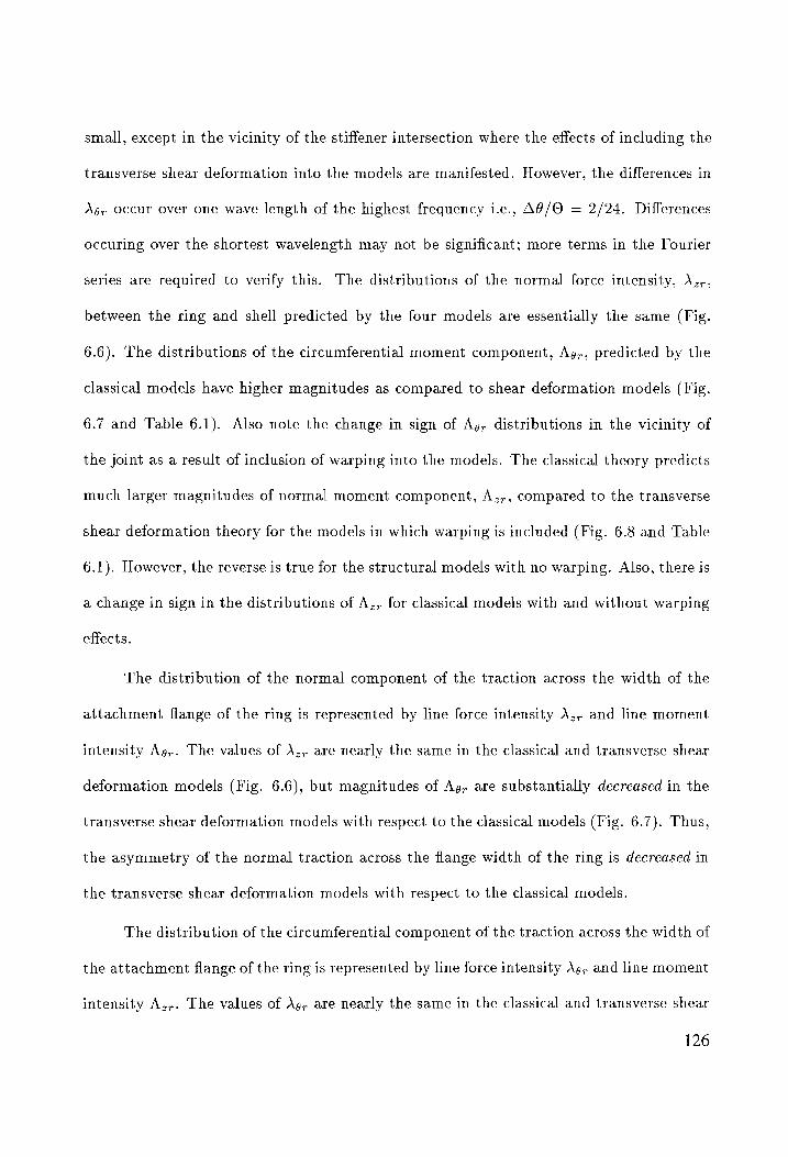
small, except in the vicinity of the stiffener intersection where the effects of including the

transverse shear deformation into the models are manifested. However, the differences in

Agr occur over one wave length of the highest frequency i.e., A@/O = 2/24. Differences

occuring over the shortest wavelength may not be significant; more terms in the Fourier

series are required to verify this. The distributions of the normal force intensity, A.,,

between the ring and shell predicted by the four models are essentially the same (Fig.

6.6). The distributions of the circumferential moment component, Ag,, predicted by the

classical models have higher magnitudes as compared to shear deformation models (Fig.

6.7 and Table 6.1). Also note the change in sign of Ag, distributions in the vicinity of

the joint as a result of inclusion of warping into the models. The classical theory predicts

much larger magnitudes of normal moment component, A,,, compared to the transverse

shear deformation theory for the models in which warping is included (Fig. 6.8 and Table

6.1). However, the reverse is true for the structural models with no warping. Also, there is

a change in sign in the distributions of A,, for classical models with and without warping

effects.

The distribution of the normal component of the traction across the width of the

attachment flange of the ring is represented by line force intensity A,, and line moment

intensity Ag,. The values of \,, are nearly the same in the classical and transverse shear

deformation models (Fig. 6.6), but magnitudes of Ag, are substantially decreased in the

transverse shear deformation models with respect to the classical models (Fig. 6.7). Thus,

the asymmetry of the normal traction across the flange width of the ring is decreased in

the transverse shear deformation models with respect to the classical models.

The distribution of the circumferential component of the traction across the width of

the attachment flange of the ring is represented by line force intensity Ag, and line moment

intensity A,,. The values of Ag, are nearly the same in the classical and transverse shear

126

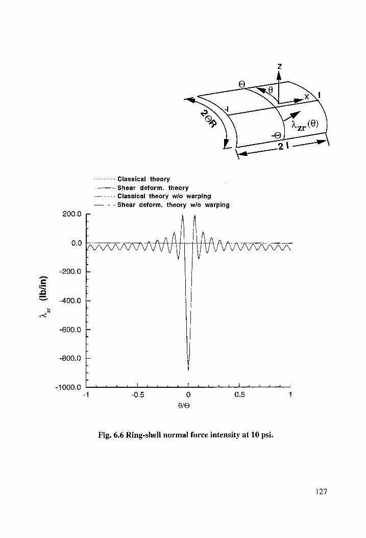
(Ib/in

) 2r

r

wee eeeee Classical theory


——.---- Classical theory w/o warping

—— - - Shear deform. theory w/o warping

200.0 |

aah Nan,

© IIIT

~200.0

-400.0

-600.0

-800.0

t T

qT |

' f

' {

t tT

J T

rT

{ tT

a | l _! a | L aun j

-0.5

L -1000.0

1 —_k

0/O

yy WAVAVAVAVAUAUAN

Fig. 6.6 Ring-shell normal force intensity at 10 psi.

127

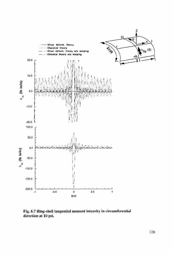
(Ib

in/i

n)

Or

A (Ib

in/in)

Or

A

20.0

10.0

-10.0 -20.0

100.0

50.0 F

ween Classical theory


—---- Classical theory w/o warping


hoa . “tims ny (i

0.0 LWA J . PAS NAINA RANA BA

-50.0 +

[ | : ; : |

-100.0 + |:

/ | r |;

150.0 |

-200.0 L111 ii Po iil “1 -0.5 0 0.5 1

Fig. 6.7 Ring-shell tangential moment intensity in circumferential

direction at 10 psi.

128

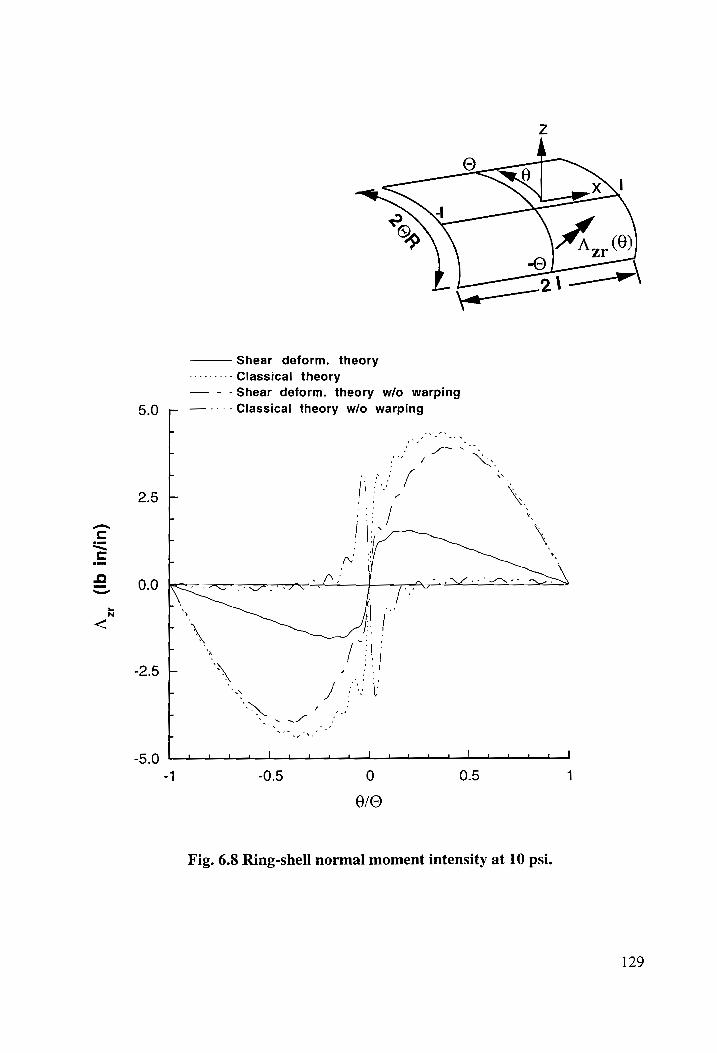
A (Ib

in/in)

zr

5.0

2.5

0.0


vttttecee Classical theory

— - -Shear deform. theory w/o warping

- —----Classical theory w/o warping

L

.

|

OE a a

NLL

1 —_—t J 1 al Ls ——

-4 -0.5 0 0.5 1

8/0

Fig. 6.8 Ring-shell normal moment intensity at 10 psi.

129

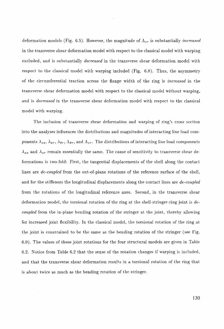
deformation models (Fig. 6.5). However, the magnitude of A,, is substantially increased

in the transverse shear deformation model with respect to the classical model with warping

excluded, and is substantially decreased in the transverse shear deformation model with

respect to the classical model with warping included (Fig. 6.8). Thus, the asymmetry

of the circumferential traction across the flange width of the ring is increased in the

transverse shear deformation model with respect to the classical model without warping,

and is decreased in the transverse shear deformation model with respect to the classical

model with warping.

The inclusion of transverse shear deformation and warping of ring’s cross section

into the analyses influences the distributions and magnitudes of interacting line load com-

ponents A,5, Ar, Aer, Agr, and A,z,. The distributions of interacting line load components

Avs and A,, remain essentially the same. The cause of sensitivity to transverse shear de-

formations is two-fold: First, the tangential displacements of the shell along the contact

lines are de-coupled from the out-of-plane rotations of the reference surface of the shell,

and for the stiffeners the longitudinal displacements along the contact lines are de-coupled

from the rotations of the longitudinal reference axes. Second, in the transverse shear

deformation model, the torsional rotation of the ring at the shell-stringer-ring joint is de-

coupled from the in-plane bending rotation of the stringer at the joint, thereby allowing

for increased joint flexibility. In the classical model, the torsional rotation of the ring at

the joint is constrained to be the same as the bending rotation of the stringer (see Fig.

6.9). The values of these joint rotations for the four structural models are given in Table

6.2. Notice from Table 6.2 that the sense of the rotation changes if warping is included,

and that the transverse shear deformation results in a torsional rotation of the ring that

is about twice as much as the bending rotation of the stringer.

130

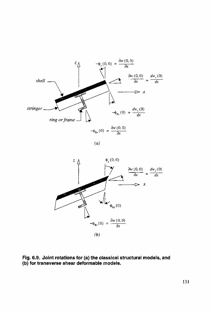
dw (0, 0) ox

Z ->, (0,0) =

\ dw(0,0) dw, (0) shell — 5 = ox ~ dx

stringer Zs dw, (0) \ (0) = —F

ring or frame

_ dw (0, 0) —o, r ( 0) - ox

(a)

Zz o,, (0, 0)

ry dw(0,0) dw, (0) ox = dx

2 ao x

aN 5, (0)

_ dw (0, 0) —9, r (0) _ a x

Fig. 6.9. Joint rotations for (a) the classical structural models, and (b) for transverse shear deformable models.

131

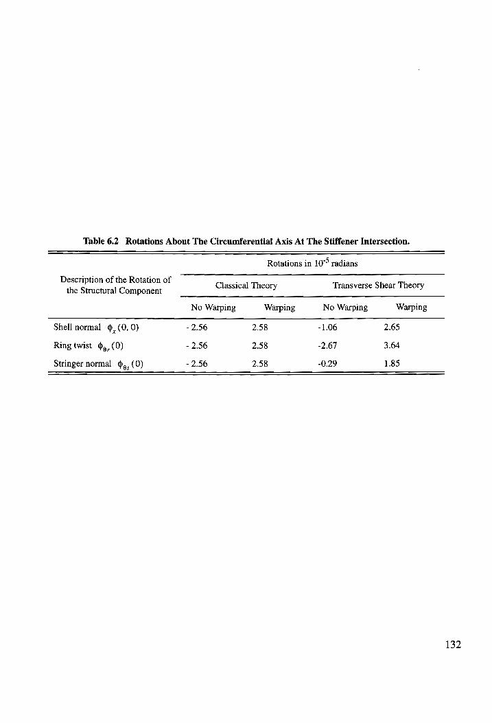
Table 6.2 Rotations About The Circumferential Axis At The Stiffener Intersection.

Rotations in 10° radians

Description of the Rotation of

the Structural Component Classical Theory Transverse Shear Theory

No Warping Warping No Warping Warping

Shell normal 9, (0, 0) - 2.56 2.58 -1.06 2.65

Ring twist $, (0) - 2.56 2.58 -2.67 3.64

Stringer normal $,. (0) - 2.56 2.58 -0.29 1.85

[32

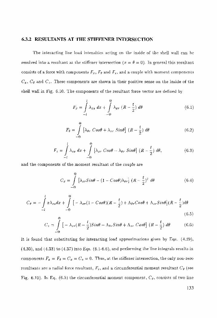
6.3.2 RESULTANTS AT THE STIFFENER INTERSECTION

The interacting line load intensities acting on the inside of the shell wall can be

resolved into a resultant at the stiffener intersection (c = 6 = 0). In general this resultant

consists of a force with components F’,, Fg and F,, and a couple with moment components

C,, Cg and C,. These components are shown in their positive sense on the inside of the

shell wall in Fig. 6.10. The components of the resultant force vector are defined by

I o

F, = Jr» da + / Aer (R- 5) d8 (6.1) —l ~O

e

Fy = / [Aer Cosd + Az, Sind] (R- 5) do (6.2) -O

©

PF, = [> dx + / [Azr Cosé — Xo, Sind] (R — 5) dO, (6.3)

—! -O

and the components of the moment resultant of the couple are

Oo

C, = / [AerSind — (1 — Cos6)Avy] (R- 5) dO (6.4) -9

l ©

Ca=- [ ered + / [ — Aer(1 — Cos0)(R - 5) + NorCos0 + AzrSin6](R - =) —i -9

(6.5) 7 t C.= / [— Awr(R— 5)Sind ~ NopSind + Mey Cost] (R~ 5) db (6.6)

-@

It is found that substituting for interacting load approximations given by Eqs. (4.29),

(4.30), and (4.33) to (4.37) into Eqs. (6.1-6.6), and performing the line integrals results in

components F, = Fy = C, = C, = 0. Thus, at the stiffener intersection, the only non-zero

resultants are a radial force resultant, F,, and a circumferential moment resultant Cg (see

Fig. 6.10). In Eq. (6.5) the circumferential moment component, C’g, consists of two line

133

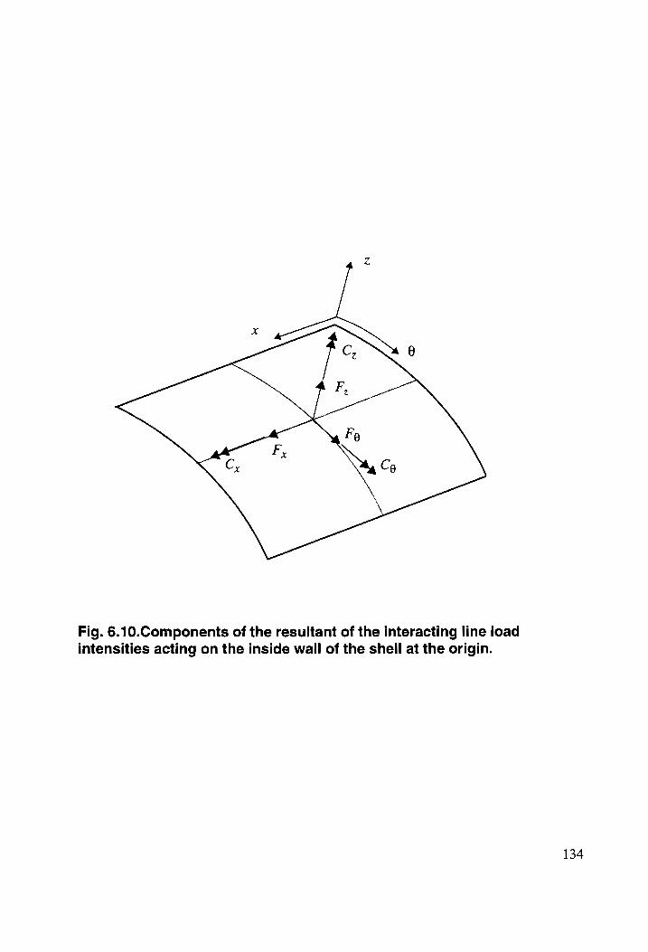
Naa ce

Fig. 6.10.Components of the resultant of the interacting line load intensities acting on the inside wall of the shell at the origin.

134

integrals; the first integral being the contribution of shell-stringer interacting loads, and

the second representing the contributions of shell-ring interacting loads. The contribution

to the radial force resultant F, in Eq. (6.3) comes only from the shell-ring interacting

load intensitites since the resultant from the stringer vanishes by Eq. (4.61).

The values of the radial force and circumferential moment resultants are computed

using Eqs. (6.3) and (6.5) for the four structural models under consideration, and are given

in Table 6.3. The differences predicted by the four structural models in the magnitudes

of the radial force resultant F, are very small, and are within 0.4% of each other. There

are substantial differences in the magnitudes of circumferential component of the moment

predicted by the four models. The values of Cg predicted by the models with warping

included are much larger than those predicted by the models without warping effects. The

individual contributions of the stringer and ring to C¢ are also affected by the change in

the model as shown in Table 6.3. It may be noted that C's is more sensitive to the effect

of warping than to transverse shear deformation.

6.3.2.1 COMPARISON OF PULL-OFF LOAD

The radial force resultant F', represents the action of the stiffeners to pull the shell

radially inward against the internal pressure load. When the stiffeners are attached to the

skin by adhesive bonding or co-curing, the adhesive joints must resist this load. The value

of F, to cause separation of the frame from the shell is called the pull-off load. Recently,

Minguet, et al.2° analyzed a finite element model of the crown panel of a fuselage in which

the stringers were allowed to pass through the joint by creating a cut-out (called a mouse

hole) in the frame. Using two sets of loading conditions, Minguet, et al. found an upper

and lower bound on the target pull-off load to be resisted by the shell-frame adhesive

joint for an ultimate cabin pressure load of 18.2 psi and an axial bulkhead reaction load

of 1110 lb/in. due to closed-end effects. For the numerical data given in Section 6.2, they

135

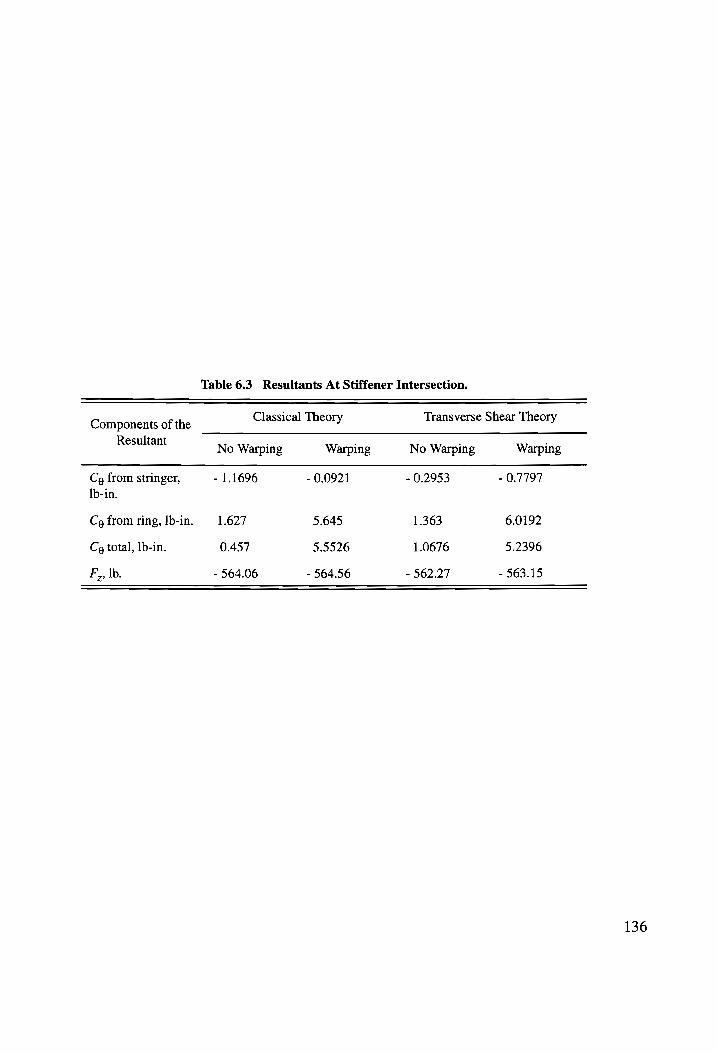
Table 6.3 Resultants At Stiffener Intersection.

Components of the Classical Theory Transverse Shear Theory

Resultant No Warping Warping No Warping Warping

Cg from stringer, - 1.1696 - 0.0921 - 0.2953 - 0.7797 Ib-in.

Cg from ring, lb-in. 1.627 5.645 1.363 6.0192

Cg total, lb-in. 0.457 5.5526 1.0676 5.2396

F,, lb. - 564.06 - 564.56 - 562.27 - 563.15

136

found these upper and lower bounds on the target pull-off load to be 1100 lbs. and 775

lbs., respectively. The values of F, obtained using the present method of analysis, and

given in Table 6.3 for the four structural models under consideration, can be multiplied

by a factor of 1.82 to predict the pull-off load for an ultimate cabin pressure load of 18.2

psi and an axial bulkhead reaction load of 1110 lb/in. due to closed-end effects. A quick

calculation shows that the present analysis predicts a target pull-off load of approximately

1025 lbs. which falls between the lower and upper bounds predicted by Minguet, et al. It

may be noted that the target pull-off load predicted by the present analysis would be a

conservative design load to start a preliminary design process.

6.3.3 SINGULAR BEHAVIOR AT THE JOINT

In Table 6.1 the comparison of peak values of the interacting line load intensities

is meant to convey the influences of transverse shear deformations and warping in the

structural modeling. The peak values of components A,,, Az,, Azr, and Ag, occur at the

joint, but these peak values do not exhibit convergence with an increasing number of terms

retained in the Fourier Series. It appears that these components are singular at the joint.

However, the resultants F, and Cg determined from these line load intensities were found

to converge quite rapidly. See Section 5.5 for further discussion of this point.

6.3.4 STIFFENER ACTIONS

The distributions of the force and moment resultants in the stiffeners are shown

in Figs. 6.11 through 6.16. The stringer axial force and bending moment distributions

(Fig. 6.11) are slightly asymmetric about the origin. The bending moment distributions

in the stringer are more sensitive to the change in models as compared to the axial force

distributions. The distribution of stringer shear force, V,,, is shown in Fig. 6.12, and it is

137

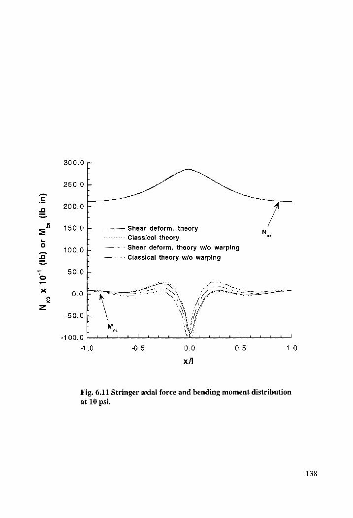
(Ib

in)

Qs

N x

10°!

(Ib)

or

M xs

300.0

250.0

t Le

| rT

Ft

1

200.0

150.0 Shear deform. theory

woceceeee Classical theory


ry rrr pr rr

|

100.0 P — ---- Classical theory w/o warping

50.0 b _

0.0

r 50.0 +

i \X -100.0 __j jt | 4 oy , Hy yy yy ld peo yy

-1.0 -0.5 0.0 0.5 1.0

x/I

Fig. 6.11 Stringer axial force and bending moment distribution

at 10 psi.

138

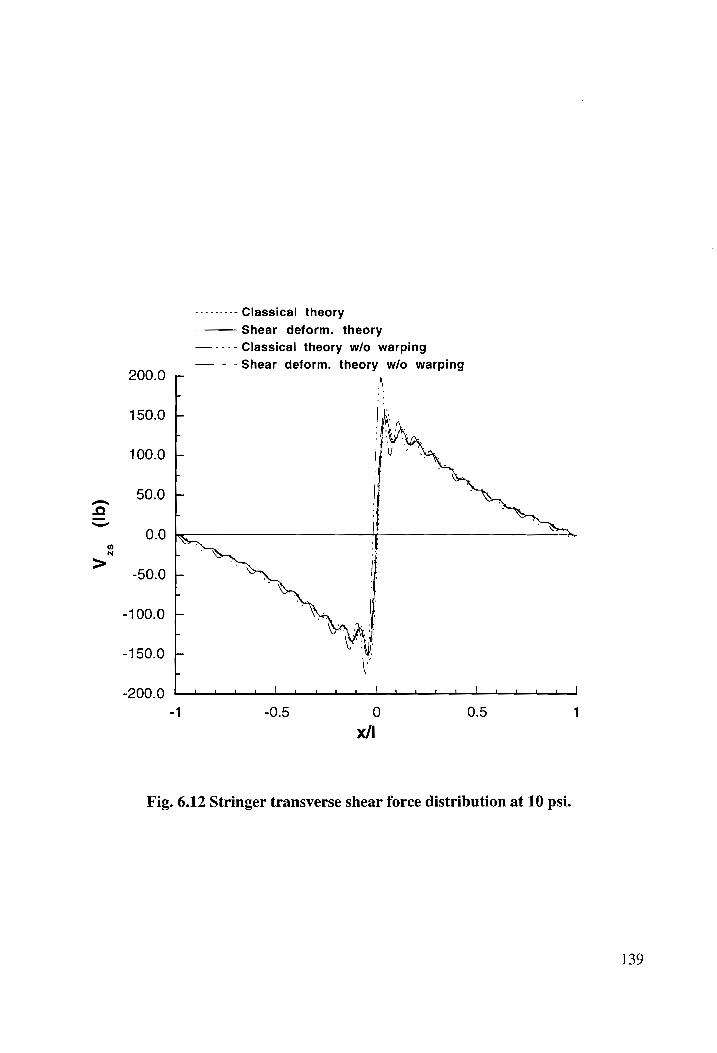
200.0

150.0

100.0

50.0

(Ib)

0.0

zs

V

-50.0

-100.0

-150.0

-200.0

vrorescee Classical theory


— ---- Classical theory w/o warping


\ . “

-

- . | a ON

\ perenne semen lees, _| | ml. aml al. al 1 J 1 i | pera ees eee, _|

1 -0.5 0 0.5 1 x/|

Fig. 6.12 Stringer transverse shear force distribution at 10 psi.

139

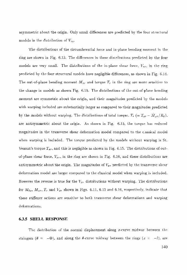
asymmetric about the origin. Only small differences are predicted by the four structural

models in the distribution of V,,.

The distributions of the circumferential force and in-plane bending moment in the

ring are shown in Fig. 6.13. The differences in these distributions predicted by the four

models are very small. The distributions of the in-plane shear force, V,,, in the ring

predicted by the four structural models have negligible differences, as shown in Fig. 6.14.

The out-of-plane bending moment M,, and torque J, in the ring are more sensitive to

the change in models as shown Fig. 6.15. The distributions of the out-of-plane bending

moment are symmetric about the origin, and their magnitudes predicted by the models

with warping included are substantially larger as compared to their magnitudes predicted

by the models without warping. The distributions of total torque, T, (= T;, — M.r/ Ro),

are antisymmetric about the origin. As shown in Fig. 6.15, the torque has reduced

magnitudes in the transverse shear deformation model compared to the classical model

when warping is included. The torque predicted by the models without warping is St.

Venant’s torque T,,, and this is negligible as shown in Fig. 6.15. The distributions of out-

of-plane shear force, V,,, in the ring are shown in Fig. 6.16, and these distributions are

antisymmetric about the origin. The magnitudes of V,, predicted by the transverse shear

deformation model are larger compared to the classical model when warping is included.

However the reverse is true for the V,, distributions without warping. The distributions

for M,,, M.,, T, and V,, shown in Figs. 6.11, 6.15 and 6.16, respectively, indicate that

these stiffener actions are sensitive to both transverse shear deformations and warping

deformations.

6.3.5 SHELL RESPONSE

The distribution of the normal displacement along z-curve midway between the

stringers (@ = —Q), and along the 6-curve midway between the rings (tx = —l), are

140

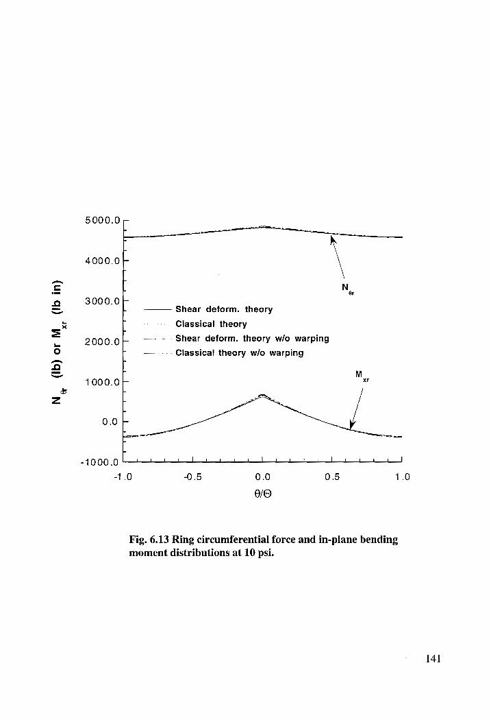
(Ib)

or Mk

(I

b in)

N Or

5000.0

4000.0

3000.0

2000.0

1000.0

-1000.0

| Ny L. Shear deform. theory

L wee erteee Classical theory

|. — - - Shear deform. theory w/o warping


r M xr

ee ee ee | ! l a | ! l | Lo _ J

0 -0.5 0.0 0.5 1.0

8/0

Fig. 6.13 Ring circumferential force and in-plane bending

moment distributions at 10 psi.

141

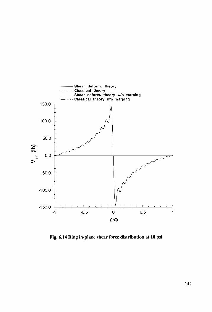
Shear deform. theory torctette Classical theory

—— - -Shear deform. theory w/o warping —.----Classical theory w/o warping

150.0 4

100.0

50.0

T T

| |

T J

J |

ft q

T I

V_,

(Ib)

-50.0 Ly

q |

T

-100.0

t re

| T -150.0 l i l J | i 1 Ld | Ls l 1 {ot n Lt I

0 0.5 1

8/0

t —_h,

t © on

Fig. 6.14 Ring in-plane shear force distribution at 10 psi.

142

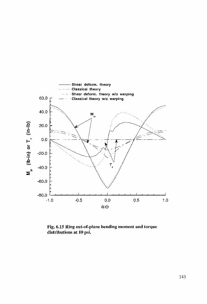
_ (in-Ib)

(Ib-

in)

or

T 2r

M

60.0

40.0

20.0

0.0

-20.0

-40.0

-60.0

-80.0


veeveeeee Classical theory



ai

mT

“yo

tL

L

L

Po | Ld Le

-1.0 -0.5 0.0 0.5 1.0

9/0

Fig. 6.15 Ring out-of-plane bending moment and torque


143

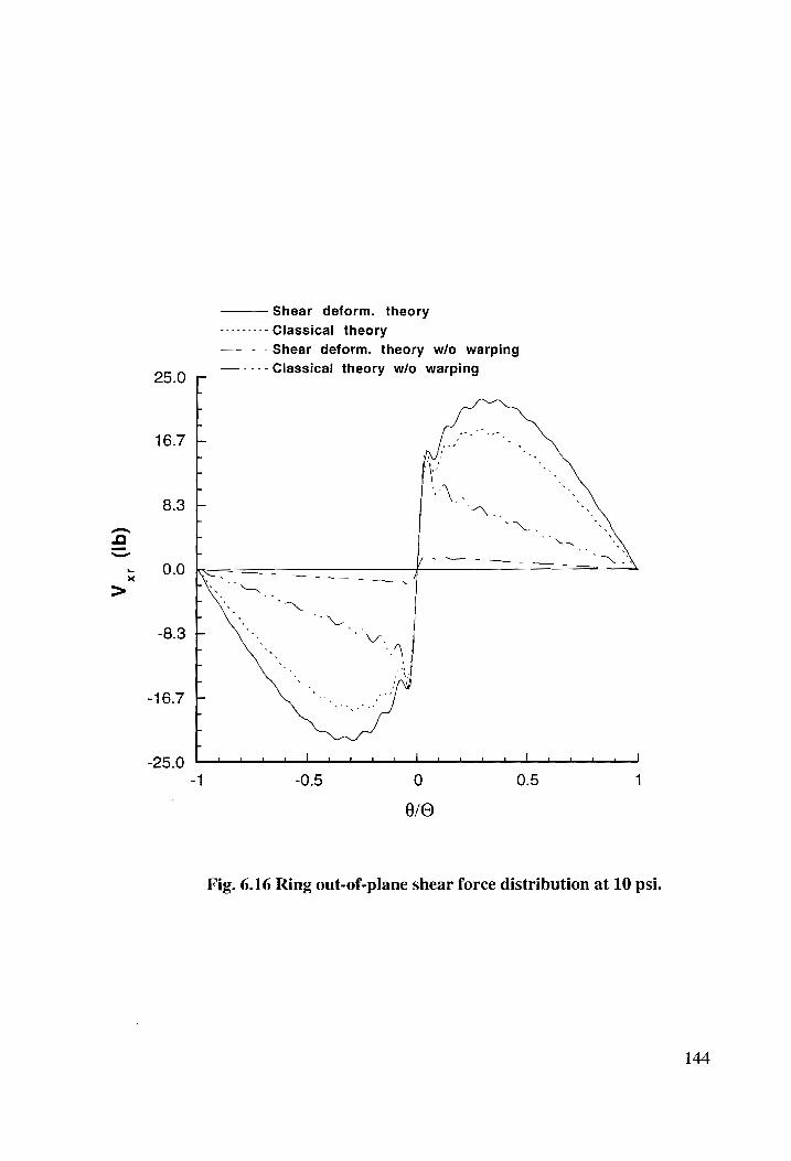
25.0

16.7

8.3

0.0

V__

(Ib)

-16.7

-25.0

[


vottrctee Classical theory


——.----Classical theory w/o warping

[

E

L

\ SO TOT —— .

[ a Ss NS

— Ms, be MN

4

P al | cede een! | J ani, el | ai | ee ee | al nk ml _, |

-1 -0.5 0 0.5 {

0/0

Fig. 6.16 Ring out-of-plane shear force distribution at 10 psi.

144

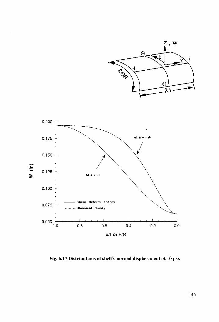
W (in)

0.200

TT

0.175

0.150

0.125

0.100

{ !

oT

{4

CT

{ T

T T

1 ct

' 1

0.075 0.050


teeeeeee - Classical theory

i | mwa | ee eel aT _|} a | al | __} _l. | | ele, | _}

-0.8 -0.6 -0.4 -0.2 0.0

x/l or 6/0

Fig. 6.17 Distributions of shell’s normal displacement at 10 psi.

145

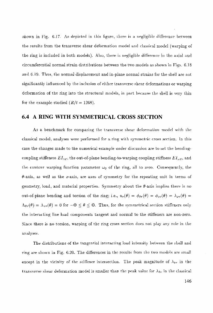
shown in Fig. 6.17. As depicted in this figure, there is a negligible difference between

the results from the transverse shear deformation model and classical model (warping of

the ring is included in both models). Also, there is negligible difference in the axial and

circumferential normal strain distributions between the two models as shown in Figs. 6.18

and 6.19. Thus, the normal displacement and in-plane normal strains for the shell are not

significantly influenced by the inclusion of either transverse shear deformations or warping

deformation of the ring into the structural models, in part because the shell is very thin

for the example studied (#/t = 1268).

6.4 A RING WITH SYMMETRICAL CROSS SECTION

As a benchmark for comparing the transverse shear deformation model with the

classical model, analyses were performed for a ring with symmetric cross section. In this

case the changes made to the numerical example under discussion are to set the bending-

coupling stiffeness EJ,,, the out-of-plane bending-to-warping coupling stiffness FI,,,, and

the contour warping function parameter wo of the ring, all to zero. Consequently, the

@-axis, as well as the z-axis, are axes of symmetry for the repeating unit in terms of

geometry, load, and material properties. Symmetry about the @-axis implies there is no

out-of-plane bending and torsion of the ring; i.e., u-(9) = or(O) = der(O) = Arr (8) =

Agr (@) = Az-(6) = 0 for -O < 6 < ©. Thus, for the symmetrical section stiffeners only

the interacting line load components tangent and normal to the stiffeners are non-zero.

Since there is no torsion, warping of the ring cross section does not play any role in the

analyses.

The distributions of the tangential interacting load intensity between the shell and

ring are shown in Fig. 6.20. The differences in the results from the two models are small

except in the vicinity of the stiffener intersection. The peak magnitude of Ag, in the

transverse shear deformation model is smaller than the peak value for Ag, in the classical

146

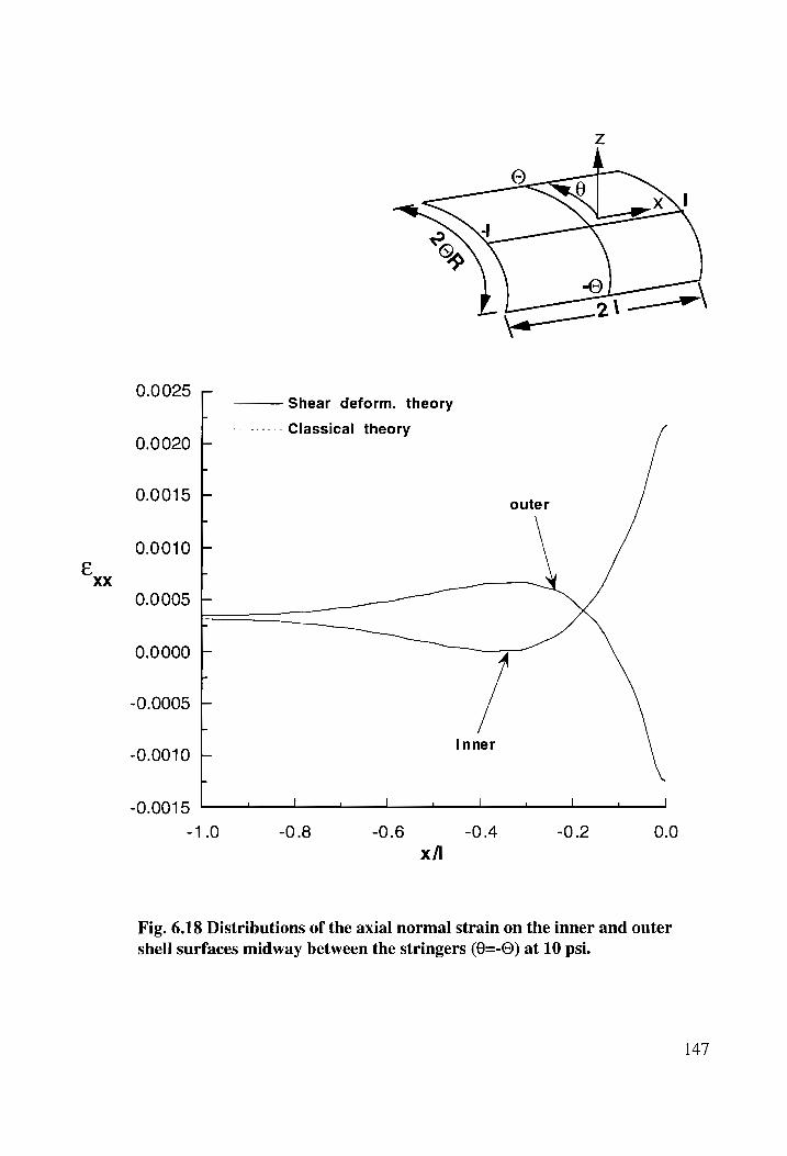
XX

0.0025

0.0020

0.0015

0.0010

0.0005

0.0000

0.0005

-0.0010

-0.0015

-1.0


so eeee eee Classical theory

-0.8 -0.6 -0.4 -0.2 0.0

Fig. 6.18 Distributions of the axial normal strain on the inner and outer

shell surfaces midway between the stringers (0=-O©) at 10 psi.

147

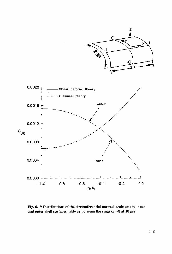
60

0.0020

0.0016

0.0012

0.0008

0.0004

0.0000


Lee eee eee Classical theory

1 i | 1 al _ el l |

-1.0 -0.8 -0.6 -0.4 -0.2 0.0

6/0

Fig. 6.19 Distributions of the circumferential normal strain on the inner

and outer shell surfaces midway between the rings (x=-/) at 10 psi.

148

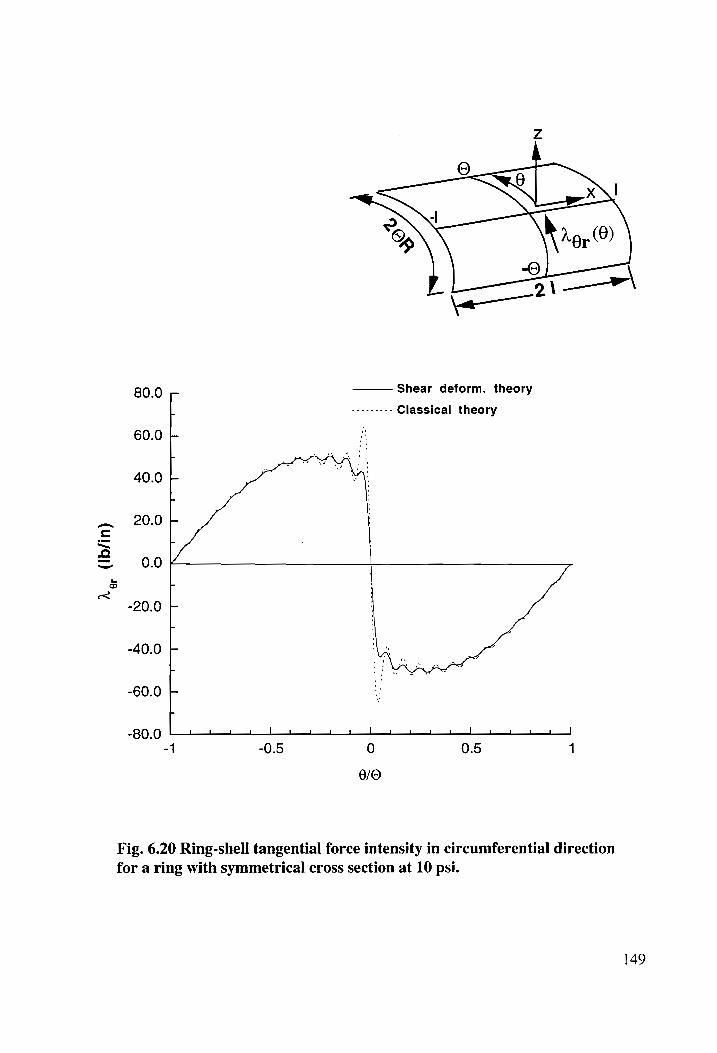
i,

(Ib/in

)

80.0

60.0

40.0

20.0

0.0

-20.0

-40.0

-60.0

-80.0


-

es Classical theory

LE

r

l 1 1 | 1 Lo i | 1 l ! | l ! i , _J

-1 -0.5 0 0.5 1

8/0

Fig. 6.20 Ring-shell tangential force intensity in circumferential direction

for a ring with symmetrical cross section at 10 psi.

149

model (50.8 lb/in versus 64.5 lb/in.). However, this difference occurs over one wave

length of the highest harmonic retained in the analysis, and may not be significant. The

distributions of the tangential and normal interacting load intensities between the shell

and stringer, and the normal load intensity between the shell and ring are not significantly

different in the two models.

For a symmetrical cross section ring, in Eqs. (6.1) through (6.6) F, = Fg = Cy, =

Cg = C, = 0. The only non-zero component of the force resultant is the radial force F,.

The values of F, computed from the classical and transverse shear deformation models

are -563.72 lb. and -561.89 lb., respectively.

6.5 SUMMARY OF RESULTS

The asymmetrical section ring complicated the analysis of the unit cell, since sym-

metry about the plane of the ring is lost. Out-of-plane bending and torsion of the ring

occur as well as a rotation of the shell-stringer-ring joint about the circumferential axis.

Inclusion of transverse shear deformations, and warping deformation of the ring’s cross

section due to torsion, into the mathematical model significantly influenced several aspects

of the response.

The sense of the rotations of the structural elements at the joint is changed with the

inclusion of warping deformation in the ring, and the twist rotation of the ring at the joint

increases by 40% with the inclusion of transverse shear deformation, as is shown in Table

6.2. That is, joint flexibility increases since element rotations at the joint are de-coupled

by using transverse shear deformation models.

The interacting loads that are strongly affected by the structural modeling are those

components associated with the asymmetric response. These are the axial force intensity

Agr, the normal moment intensity A,,, and the tangential moment intensity Ag,, between

150

the ring and shell. At the joint the magnitude of A,, is increased by the inclusion of

warping and reduced by the inclusion of transverse shear (Fig. 6.4). The normal moment

intensity A,, is a measure of the asymmetry in the distribution of the circumferential

traction across the width of the ring’s attachment flange. The sense of A,, is changed

when both transverse shear and warping are included, and its magnitudes are reduced

by the transverse shear effect (Fig. 6.8). However, the magnitude of the resultant of

the circumferential traction across the flange width of the ring, as measured by the line

load intensity Ag,, is only moderately affected by the changes in the structural models

(Fig. 6.5). The tangential moment intensity Ag, is a measure of the asymmetry in the

distribution of the normal traction across the width of the ring’s attachment flange. At the

joint, the sense of Ag, is changed by the inclusion of warping deformation and additionally

its magnitude is reduced by the inclusion of transverse shear deformation (Fig. 6.7).

However, the magnitude of the resultant of the normal traction across the flange width,

as measured by the line load intensity A,,, is essentially unaffected by changes in the

structural models (Fig. 6.6).

The distributions of the normal actions between the shell and stiffeners (Az5, Azr, and

Ag,) all show significant magnitudes only in the vicinity of the joint, with much smaller

magnitudes away from the joint. In fact, they all appear to exhibit singular behavior at the

joint, but only finite magnitudes are represented by the truncated series approximations.

The distributions of the actions tangent to the stiffeners (Azs, Ag,, and A,,), on the other

hand, have small magnitudes in the vicinity of the joint and larger magnitudes away from

the joint. These tangential actions do not exhibit singular behavior. (These results are

similar to those found for the symmetric stiffeners problem discussed in Chapter 5.)

In spite of the singular behavior of the line load intensities associated with the normal

actions, the resultant of these distributions resolved at the joint converge relatively quickly

151

with the number of terms retained in the series approximations. The resultant consists

of a radial force F, and a moment Cs, about the circumeferential axis. F, represents the

action of the stiffeners to pull the shell radially inward against the pressure load, and

Cg is primarily due to asymmetry in the actions between the ring and shell. Force F, is

essentially unaffected by the structural modeling (Table 6.3), and its magnitude for the

example studied is about 17% of the total pressure load carried by the unit cell. The

remaining pressure load is carried by the shell itself. The moment C’g is very sensitive to

the structural modeling, in particular to the effect of warping as shown in Table 6.3. This

moment C’, vanishes for a completely symmetric problem.

The out-of-plane bending moment and torque in the ring are very sensitive to the

structural modeling, as might be expected. The magnitudes of the both the out-of-plane

bending moment and torque increase with the inclusion of warping and transverse shear

into the mathematical model (Fig. 6.15). However, the shell’s normal displacement and

strains are insensitive to the changes in the structural models for the very thin shell

(R/t = 1268) used in the numerical example.

152

CHAPTER 7

CONCLUDING REMARKS

7.1 SUMMARY

Structural analyses are developed to determine the linear elastic and geometrically

nonlinear elastic response of an internally pressurized, orthogonally stiffened cylindrical

shell. The structural configuration is of a long circular cylindrical shell stiffened on the

inside by a regular arrangement of identical stringers and identical rings. Periodicity of

this configuration permits the analysis of a unit cell model consisting of a portion of the

shell wall centered over one stringer-ring joint; i.e., deformation of a structural unit cell

determines.the deformation of the entire stiffened shell. See Fig. 1.1. The stringer-ring-

shell joint is modeled in an idealized manner; the stiffeners are mathematically permitted

to pass through one another without contact, but do interact indirectly through their

mutual contact with the shell at the joint. The stiffeners are modeled as discrete beams.

The stringer is assumed to have a symmetrical cross section and the ring either a symmetric

or an asymmetric open section.

The formulations presented for the linear elastic response include the effect of trans-

verse shear deformations and the effect of warping of the ring’s cross section due to torsion.

These effects are important when the ring has an asymmetrical cross section, because the

loss of symmetry in the problem results in torsion of the ring, as well as out-of-plane

bending, and a concomitant rotation of the joint at the stiffener intersection about the

circumferential axis. Restraint of cross-sectional warping, as occurs here in the ring due

to contact with the shell, is an important contributor to the normal stresses in thin-walled

open section bars. Based on transverse shear deformations and cross-sectional warping

153

of the ring, four structural models are defined. The simplest model uses non-transverse-

shear-deformable theory, or classical theory, and neglects warping due to torsion. The

most complex model includes both effects. Models of intermediate complexity occur for

inclusion of one effect without the other. The formulations presented for the geometrically

nonlinear response take into consideration only the symmetrical cross section of stiffeners,

and are based on classical structural theories.

For all the structural models, the response of the unit cell under internal pressure is

obtained by utilizing the Ritz method. Displacements are assumed as truncated Fourier

Series plus simple terms in the axial coordinate to account for the closed-end pressure

vessel effect. Equilibrium is imposed by virtual work. Pointwise displacement continuity

between the shell and stiffeners is achieved by Lagrange multipliers which represent the

interacting line load distributions between the stiffeners and the inside shell wall (see

Fig. 1.2). Data from a composite material crown panel typical of a large transport

fuselage are used for two numerical examples. The first numerical example is used to

validate the structural model, and also to compare the linear response and geometrically

nonlinear response of the unit cell model with symmetrical section stiffeners. In the second

numerical example the linear elastic response of the unit cell model with an asymmetrical

cross section ring is analyzed.

7.2 CONCLUDING REMARKS

7.2.1 EFFECT OF GEOMETRIC NONLINEARITY

It is found that the spatial distribution of the normal displacements of the cylindrical

shell are more uniform, and the bending strains are reduced, in the geometrically nonlinear

elastic analysis with respect to what is predicted by the linear elastic analysis. That is,

pillowing of the skin is reduced by the inclusion of geometric nonlinearity into the analysis.

154

However, in the nonlinear analysis the most severe circumferential bending is confined to a

narrow boundary layer adjacent to the stringer midway between the rings, and the interior

portion of the shell behaves as a membrane. In the linear analysis the bending occurs over

the entire circumference of the shell. The development of the bending boundary layer

due to the inclusion of geometric nonlinearity into the analysis causes an increase in the

circumferential transverse shear resultant in the shell adjacent to the stringer compared

to the linear analysis. Increased interlaminar shear stresses can be expected as a result of

the increased transverse shear resultant.

The axial force carried by the stringer due to the closed-end pressure vessel effect is

increased in the nonlinear analysis with respect to its value in the linear analysis. Also,

the circumferential force carried by the ring is increased in the nonlinear analysis with

respect to its value in the linear analysis. Thus, the stiffeners resist an increased portion

of the internal pressure load, accompanied by a commensurate decrease in the load carried

by the shell, when geometric nonlinearity is included into the analysis.

7.2.2 INFLUENCE OF AN ASYMMETRICAL SECTION RING

The asymmetrical section ring complicated the analysis of the unit cell, since sym-

metry about the plane of the ring is lost. Inclusion of transverse shear deformations,

and warping deformation of the ring’s cross section due to torsion, into the mathematical

model significantly influenced several aspects of the response. The interacting loads that

are strongly affected by the structural modeling are those components associated with

the asymmetric response. These are the axial force intensity Az;, the normal moment

intensity A,,, and the tangential moment intensity Ag, between the ring and shell. At the

joint the magnitude of A,, is increased by the inclusion of warping and reduced by the

inclusion of transverse shear (Fig. 6.4). The normal moment intensity A,, is a measure

of the asymmetry in the distribution of the circumferential traction across the width of

155

the ring’s attachment flange. The sense of A,, is changed when both transverse shear and

warping are included, and its magnitudes are reduced by the transverse shear effect (Fig.

6.8). However, the magnitude of the resultant of the circumferential traction across the

flange width of the ring, as measured by the line load intensity Ag,, is only moderately

affected by the changes in the structural models (Fig. 6.5). The tangential moment inten-

sity Ag, is a measure of the asymmetry in the distribution of the normal traction across

the width of the ring’s attachment flange. At the joint, the sense of Ag, is changed by the

inclusion of warping deformation and additionally its magnitude is reduced by the inclu-

sion of transverse shear deformation (Fig. 6.7). However, the magnitude of the resultant

of the normal traction across the flange width, as measured by the line load intensity A.,,

is essentially unaffected by changes in the structural models (Fig. 6.6).

The sense of the rotations of the structural elements at the joint is changed with the

inclusion of warping deformation in the ring, and the twist rotation of the ring at the joint

increases by 40% with the inclusion of transverse shear deformation, as is shown in Table

6.2. That is, joint flexibility increases since element rotations at the joint are de-coupled

by using transverse shear deformation models.

The out-of-plane bending moment and torque in the ring are very sensitive to the

structural modeling, as might be expected. The magnitudes of the both the out-of-plane

bending moment and torque increase with the inclusion of warping and transverse shear

into the mathematical model (Fig. 6.15). However, the distributions and magnitudes

of the normal displacement and strains of the shell midway between the stiffeners are

unaffected by the change in the structural models.

156

7.2.3 SINGULARITY AT THE SHELL-STRINGER-RING JOINT

The distributions of the normal actions between the shell and stiffeners (As, Azr, and

Ag,) all show significant magnitudes only in the vicinity of the joint, with much smaller

magnitudes away from the joint. In fact, they all appear to exhibit singular behavior at the

joint, but only finite magnitudes are represented by the truncated series approximations.

The distributions of the actions tangent to the stiffeners (A;;, Agr, and Az,), on the other

hand, have small magnitudes in the vicinity of the joint and larger magnitudes away

from the joint. These tangential actions do not exhibit singular behavior. In spite of

the singular behavior of the line load intensities associated with the normal actions, the

resultant of these distributions resolved at the joint converge relatively quickly with the

number of terms retained in the series approximations (e.g., see Fig. 5.17). The resultant

consists of a radial force F, and a moment C's about the circumferential axis (see Fig.

6.10). F, represents the action of the stiffeners to pull the shell radially inward against

the pressure load, and C’g is primarily due to asymmetry in the actions between the ring

and shell. The magnitude of force F, represents the portion of the total pressure load

carried by the stiffeners. The remaining pressure load is carried by the shell itself. Force

F,, is essentially unaffected by the structural modeling (Table 6.3). The moment Cs is

very sensitive to the structural modeling, in particular to the effect of warping as shown

in Table 6.3. This moment C's vanishes for a completely symmetric problem.

The series for the interacting normal load intensity \,, at the stiffener intersection

does not appear to converge even in the geometrically nonlinear analysis. However, the

Fourier Series for the total radial resultant load carried by the stiffeners, which is resolved

at the intersection, exhibits rapid convergence in the geometrically nonlinear analysis (see

Fig. 5.18). The total radial resultant load carried by the stiffeners is slightly increased in

the geometrically nonlinear analysis with respect to its value in the linear analysis.

157

7.3 RECOMMENDATIONS FOR FUTURE WORK

The analysis could be extended to include the important load cases of torsion and

bending in addition to internal pressure. Torsion of the stiffened shell is equivalent to

a shear load of the unit cell, and this loading case corresponds to an antisymmetric de-

formation pattern of the unit cell model. Bending is somewhat more complex since the

displacement field has period of 27 rather than the periodicity of the stringer spacing.

Singular solutions can be investigated to improve the solution methodology. To

begin with, the simplest configuration can be analyzed; i.e., consider the linear response

of a classical structural model with symmetric section stiffeners. This problem can be

reformulated in terms of four integral equations in which the unknowns are the magnitudes

of the interacting load components Azs(r), Azs(z), Agr(O), and Az-(@). These integral

equations are associated with either the tangential or normal displacement constraints

between the shell and stiffeners. The kernels to these equations are Green’s functions

(or influence functions), which are displacement solutions to the shell, stringer, and ring

problems under the actions of concentrated forces. This approach is appealing because

the solution reduces to solving for the interacting load components in integral expressions

along the contact lines rather than solving for the displacements and interacting loads

over the entire solution domain. The difficulty with this approach is in obtaining the

Green’s functions, and solving singular integral equations that may result from the contact

problems.

158

REFERENCES

INiu, M. C-Y., Airframe Structural Design, Conmilit Press Ltd., Hong Kong, 1988,

pp. 520-526.

*Jackson, A. C., Campion, M. C., and Pei, G., “Study of Utilization of Ad-

vanced Composites in Fuselage Structures of Large Transports,” NASA Contractor Report

172404, Contract NAS1-17415, September, 1984.

2Rouse, N. E., “Making Reliable Joints in Composites,” Machine Design, March,

1985, pp 79-82.

*Cole, R. T., Batch, E. J., and Potter, J., “Fasteners for Composite Structures,”

Composites, Vol. 13, 1982, pp. 233-240.

*Tlcewicz, L. B., Smith, P. J., and Horton, R. E., “Advanced Composites Fuse-

lage Technology,” Proceedings of the Third NASA/DoD Advanced Composites Technology

Conference, NASA CP-3178, 1992, pp. 97-156.

Swanson, G. D., Ilcewicz, L. B., Walker, T. H., Graesser, D., Tuttle, M., and

Zabinsky, Z., “Local Design Optimization for Composite Transport Fuselage Crown Pan-

els,” Proceedings of the Second NASA/DoD Advanced Composites Technology Conference,

NASA CP-3154, 1992, pp. 243-262.

“Jackson, A. C., “Development of Textile Composite Preforms for Aircraft Struc-

tures,” Proceedings of the AIAA/ASME/ASCE/AHS/ASC 35th Structures, Structural

Dynamics and Materials Conference (Hilton Head, SC), Part 2, AIAA, Washington, D.C.,

April 1994, pp. 1008-1012.

8Grigoluk, E., and Tolkachev, V., Contact Problems in the Theory of Plates and

shells, Mir Publishers, Moscow, English Translation, 1987, pp. 5, 129-191, 328-395.

°Melan, E., “Ein Beitrag zur Theorie geschweisster Verbindungen,” Ing.-Arch., Vol.

3, No. 2, 1932, pp. 123-129.

159

Buell, E. L., “ On the Distribution of Plane Stress in a Semi-infinite Plate with

Partially Stiffened Edge,” Journal of Math and Physics, Vol. 26, No. 4, 1948, pp. 223-233.

11 Koiter, W. T., “Diffusion of Load from a Stiffener into a Sheet,” Quarterly Journal

of Mechanics and Applied Math., Vol. 8, No. 2, 1955, pp. 164-178.

12Benscoter, S. U., “Analysis of a Single Stiffener on an Infinite Sheet,” Journal of

Applied Mechanics, Vol. 16, No. 3, 1949, pp. 242-246.

'SBudiansky, B., and Wu, Tai Te, “Transfer of Load to a Sheet from a Rivet-

attached Stiffener,” Journal of Math and Physics, Vol. 40, No. 2, 1961, pp. 142-162.

4Pischer, F. J., “Stress Diffusion from Axially Loaded Stiffeners into Cylindrical

Shells,” International Journal of Solids & Structures, Vol. 4, 1968, pp. 1181-1201.

5 Fligge, W., “Stress Problems in Pressurized Cabins,” NACA Technical Note

2612, 1952.

16 Houghton, D. S., “The Influence of Frame Pitch and Stiffness on the Stress Distri-

bution in Pressurized Cylinders,” CoA Note No. 79, The College of Aeronautics, Cranfield,

February, 1958.

l?Williams, D., “Pressure-Cabin Problems,” An Introduction to the Theory of Atr-

craft Structures, Edward Arnold Ltd., 1960, pp. 283-321.

18Wang, J. T-S., “Orthogonally Stiffened Cylindrical Shells Subjected to Internal

Pressure,” AIAA Journal, Vol. 8, March, 1970, pp. 455-461.

19Wang, J. T-S., and Hsu, T-H., “Discrete Analysis of Orthogonally Stiffened Com-

posite Cylindrical Shell,” AIAA Journal, Vol. 23, No. 11, 1985, pp. 1753-1761.

20Boitnott, R. L., “Nonlinear Response and Failure Characteristics of an Internally

Pressurized Composite Cylindrical Panels,” Doctoral Dissertation, Engineering Science

and Mechanics Department, Virginia Polytechnic Institute and State University, Blacks-

burg, Virginia, March 1985, pp. 82-97, 104-117.

160

21 The ABAQUS Theory Manual, Version 5.3, Hibbitt, Karlsson and Sorensen, Inc.,

Rhode Island, 1993.

*2MacNeal, R. H., The NASTRAN Theoretical Manual, The MacNeal-Schwendler

Corporation, California, 1972.

23 Hoff, N. J., “The Applicablity of Saint-Venant’s Principle to Airplane Structures,”

Journal of Aeronautical Science, Vol. 12, 1945, pp. 455-460.

24Novozhilov, V. V., Thin Shell Theory, Noordhoff Ltd., The Netherlands, 1964,

pp. 23.

*5 Jones, R. M., Mechanics of Composite Materials, Scripta Book Co., Washington

DC, 1975, pp. 51, 154, 155.

6 Vasiliev, V. V., Mechanics of Composite Structures, Taylor & Francis Ltd., Wash-

ington DC, 1993, pp. 62-71.

27 Cohen, G. A., “Transverse Shear Stiffness of Laminated Anisotropic Shells,” Com-

puter Methods in Applied Mechanics and Engineering, Vol. 13, 1978, pp. 205-220.

28Woodson, M. B., Johnson, E. R., and Haftka, R. T., “A Vlasov Theory for

Laminated Composite Circular Beams with Thin-walled Open Sections,” Proceedings of

the AIAA/ASME/ASCE/AHS/ASC 34th Structures, Structural Dynamics and Materials

Conference (LaJolla, CA), Part 5, AIAA, Washington, D.C., April 1993, pp. 2742-2760.

22Woodson, M. B., “Optimal Design of Composite Fuselage Frames for Crashwor-

thiness,” Doctoral Dissertation, Department of Aerospace and Ocean Engineering, Vir-

ginia Polytechnic Institute and State University, Blacksburg, Virginia, December 1994,

pp. 17-71.

20Bauld, N. R., Jr., and Tzeng, L., “A Vlasov Theory for Fiber-Reinforced Beams

with Thin-walled Open Cross-Sections,” International Journal of Solids & Structures, Vol.

20, No. 3, 1984, pp. 277-297.

161

3!Sanders, J. L., “An Improved First-Approximation Theory for Thin Shells,”

NASA Technical Report R-24, June, 1959.

32Sanders, J. L., “Nonlinear Theories for Thin Shells,” Quarterly of Applied Math-

ematics, Vol. 21, No. 1, 1963, pp. 21-36.

33Minguet, P. J., Fedro, M., O’Brien, T. K., Martin, R., Ilcewicz, L., Awerbuch, J.,

and Wang, A., “Development of a Structural Test Simulating Pressure Pillowing Effects

in a Bonded Skin/Stringer/Frame Configuration,” Proceedings of the Fourth NASA/DoD

Advanced Composites Technology Conference, NASA CP-3229, 1993, pp. 863-880.

162

=

B;;

i]

er

€s

Exxr, €66, Ezz

€xO, €Oz, Exz

Mm

M

Mur

Mes

Mor

Mor, Mee, Mor, Mere

Nor

Nurs

Neg, Nee, Nec; Nx

8 £0

NOMENCLATURE

Laminate extensional stiffness

Laminate extension-bending coupling stiffness

Laminate bending stiffness

Eccentricity of ring

Eccentricity of stringer

Three-dimensional engineering normal strains

Three-dimensional engineering shear strains

Harmonic in axial direction

Number of harmonics in axial direction

Ring bimoment

Stringer bending moment

Ring in-plane bending moment

Stress couples of shell theory

Stress couple of Sanders’ theory of shells

Modified stress couples of transverse shear

deformation shell theory

Ring out-of-plane bending moment

Harmonic in circumferential direction

Number of harmonics in circumferential direction

Ring circumferential force

Stringer axial force

Stress resultants of shell theory

Stress resultant of Sanders’ theory of shells

Internal pressure load

163

Qi;

Qe, 6

Ro

2RO

2l

Ur

Us

Uz, Uy, Uz

zr

éwW

Wr

Am

Bn

Car

Stringer axial load share

Transformed reduced stiffness of lamina

Transverse shear resultants for shell

Radius to middle surface of shell

Radius to the reference arc of ring

Area of the shell’s reference surface

Thickness of shell

Stringer spacing

Frame, or ring, spacing

Torque in the ring

Axial displacement of middle surface of shell

Axial displacement of reference arc of ring

Axial displacement of centroidal axis of stringer

Rigid body displacements

Circumferential displacement of middle surface of shell

Circumferential displacement of reference arc of ring

Stringer shear force

Ring in-plane shear force

Ring out-of-plane shear force

Virtual work

Normal displacement of middle surface of shell

Normal displacement of reference arc of ring

Normal displacement of centroidal axis of stringer

Axial frequency

Circumferential frequency

Normal strains of ring’s reference axis

164

€rs

€xxr, €66

Orr, F986

Tr6,Frz,F6z

Vers Yer

Yes

Yxre

Yar, Vez

KGs

Karr

Ker

Ker, 66

Kind, Kad

&

Kr

Agr, Abr, Azr

Nor, Agr

Acs, Azs

Po

Per

Pos

Or

Par

Pz

Per

Tr

Q,, Qy, Q,

Normal strains of stringer’s centroidal axis

Normal strains of shell’s middle surface

Normal stress components

Shear stress components

Ring’s transverse shear strains

Stringer’s transverse shear strain

In-plane shear strain of shell’s middle surface

Transverse shear strains of shell’s middle surface

Bending curvature of stringer’s centroidal axis

In-plane bending curvature of ring’s reference axis

Out-of-plane bending curvature of ring’s reference axis

Bending strains of shell’s middle surface

Twisting strains of shell’s middle surface

Twisting strain of shell’s middle surface in Sanders theory

Shell-ring interacting force intensities (F/L)

Shell-ring interacting moment intensities (F-L/L)

Shell-stringer interacting force intensities

Rotation of shell’s normal about z-axis

Torsional rotation of ring

Bending rotation of stringer

Rotation of shell’s normal about 6-axis

In-plane bending rotation of ring

Shell’s rotation around normal

Out-of-plane bending rotation of ring

Twist rate of ring

Rigid body rotations

165

APPENDIX A

ELEMENTS OF MATRICES FOR LINEAR ANALYSIS USING

TRANSVERSE SHEAR DEFORMATION MODEL

The non-zero elements of the submatrices K;;, Bj; and Fy, in Eq. (4.68) for the trans-

verse shear deformation model are listed below. The parameter 6;; is Kronecker delta assuming

the values zero for 2 # 7, and one for ¢ = 7, respectively.

Elements of (10MN +3M43N +42) x (1OMN +3M+4+3N +2) submatrix [411]

Ky (1, 1) =

Ki (1, 2)

Kit (2, 2) =

Iu (3,3)

Ky1 (3,4)

Ky, (3,5)

Kn (4,4)

Ky, (4,5) =

Ky (5,5)

Ku, (6,6)

Ku (6,7)

Ky, (6,8) =

Ky 1 (7, T=

Ku (7,8) =2

A110R

i

=2A120R

4Ax2.0l

R

=2A1107, lORSinp

=2A120mlOSmp

=2Bi07 lORSmp

Ag2 =2( RR + Aga a? lO Rbmp

=9( 72 — A4g)OmlO Rb mp

=2(Ag4 + Dy,07, ORS mp

=o 42 Ago 2 2 1 Ass

A A =2( + 435.10

B 2(— an ~ Ass lObng

yd 4 AS 2 Obng

Bo ( R

F084

_ Ass \BnlOdbng

166

Ky, (8,8)

Ky (9,9)

Ay, (9,12) =

Ay, (9,14)

Ky, (9,15)

K11 (9, 18)

Ki (11, 11)=

Ay (11, 13) =

Ki (11, 16)

Ky (11,17) =

Ay, (18, 13)

Ky, (13, 16)

Ky (13,17)

Ky, (15,15)

Ky, (15, 18)

Ky (17,17)

=|Bo + Bég — Bég +

=[ mm t

=(Bi2 _ A4gR)amlObmpbng = —Ky4 (14, 15)

=[Aga + Diaz, +

= [Ass + =>

Doo =2(F- Bn + Ass R)Obng

A “uo! ns 6 Bi ]lObmpbng = Kix (10, 10)

Bi, — B ~[Ai2 + Aes + , Bh By, OmBnrlObmpbng = —~Ky1 (10,11)

R

=—Ay2AmOlémpbng = —Kyy (10, 13)

1 _ Pp

=[Byj02, + (Bes = Bos) 2119 ps. 55ng = Ky, (10,16) R2

=—(Biz + Bég + Bég)amBnlOSmpSng = —K11 (10,17)

A as 2(Bl. — B? D}} - 2D22 D2? {4 722 G2 55 (Bée és) , ( 66 — + 66) a2 he + | Age + R R

RIObmpbn¢ = Ki (12, 12)

A (Ae FA) 6, Ob mpbng = Ky, (12,14)

(Dai — 2D}2 + D22 a8) R Om Bn! Ob npbng

= —Ky (12,15) _{ Ba B2 — Ass + [( Bag + Bog)R+ DU - D8] 02, }1Obmpbng

= Ky, (12,18)

An | A = arr + Aqga?, | RIOSmpSng = Ky (14,14)

B =~(As55 — Fp Bul Obmpbng = = Ky, (14,18)

(Dik — 2D}2 + D2 R?

3. 7 R1Obmpbng = Was (16, 16)

=—(D3b + Diz — D22)0mBnlObmpong = —K1 (16,17)

<u =? g? + (DE + 2DB + D22)a?,] RIOSimpSng = Kir (18,18)

167

Elements of (6M +1) x (6M +1) submatrix [K2.|

(EA)s

2l

Ko (2, 2) =(EA),02, [mp

Koo (1, 1) =

Ko2 (3,3) =(EA),07,16mp

Ko2 (4,4) =(GA),a7, lémp

Koo (5,5) =(GA) 502, lbmp

Koo (6,6) =|(GA)s + (Elgg) 507, |lSmp

Ko (7,7) =[(GA)s + (Flog) 50%, |lémp

Elements of (6N + 1) x (6N +1) submatrix [K33]

2E AO

Ro

K'33 (2,2) =C Age? bag Ro

K33 (1, 1) =

K'33 (2,7) =-GAzeBnO6ng

K33 (3,3) =(F AG? + GAse) 5 One

K33 (3,4) =(EA + GAgg Bn bn

K33 (3,6) =-GAzeO6ng

Kg (4,4) =(BA + GAs 2) 2b K33 (4,6) =-GAz6BnO6nq

2Elye — Eliw 9.49] © — by, Rant Re Ban] One , K33 (5,5) = Elz: + (GJ +

Elue

Ro

Kaa (5,7) =— (Gu + Elz, +

33 (5, 6) =(Elir + 2) FE Obng

Ely:

Ro

El, : = Odn )+ (p= + R i) q

168

0

0

El, 2

Ro ° Ro QE Ios ELou K33 (7,7) = (GJ + GAgo Ro) + (Elez + “Ryo Re

K33 (6,7) =-(Elze +

0

2 ————

Bn Ro Ong

Elements of (10MN+3M +3N +2) x 4M submatrix [B,]

(=1)" Om,

By, (3,1) =-lén»

By (,1)=

Byy (4,4) =—l6 np

Bry (5,1) =5lémp

By (9,2) =—lbmp

By, (10,1) =—l8 ap

By (13,4) =—lbinp

By (14,3) =—[6inp

Bu (15,1) = Sl mp t

Bry (16,2) =515mp

Elements of (10MN+3M +3N +2) x (5N +1) submatrix [B,,]

By (2,1) =-2a0

By. (4,1) =-2a0

Bie (6,3) =-a06n,

By (7,4) =-aO bn,

, ¢ Br» (8,3) = 520 6ng

169

By (9,2) =-aObn,

By (11,3) =-aO6,,,

Byy (12,6) =-a,aObn,q

By (13,4) =—-aOby,

By (14,5) =apaOdn,g

By (15,2) = 5008,

Byo (17,3) = 500 8ng t

By, (18,6) = 57% ptObng

Elements of (10M N +3M+3N +2) x 1 submatrix [B,3|

By3 (1,1) =1

Elements of (6M +1) x 4M submatrix [B2|

—1 m+ 1

By je Am

Bo, (2,1) =lémp

Boy (3,2) =lédmp

Bo (4,3) =l6mp

Boy (5,4) =lbmp

Bo, (6,1) =lesdmp

Bo (7, 2) =lésdmp

170

ix [Bo3] atrix | M+1)x1subm f (6 ts o Elemen

—1 1 1) = Bos (1,

1x [B32] trix [ bma su 1) x (5N +1) + f (6N nts o Eleme

9 B3y (1,1) =2a

ébng B32 (2,2) =aQ)

dng Ba (3,3) =aO

bng Bs (4, 4) =aQ

Odbng (5,2) =e,a Ba , soe.

B39 (5,3) ~ Ro

bng (5,5) =aO B32 , —

B32 (5,6) = Ro

Odbng (6,3) =e,a B39

B39 (7, 3) ~~ Ro AD Ong

B 6) =(1— ie

ements o . | . + ix [Fi E _ bmatrix [F 1 su 2) x 3N 3M N f (10M ts ]

70 Fy (1) =pR

1OR Fy (2) =4p

17]

APPENDIX B

ELEMENTS OF MATRICES FOR LINEAR ANALYSIS

USING CLASSICAL MODEL

The non-zero elements of the submatrices K;;, Bj; and Fy, in Eq. (4.68) for the classical

model are listed below. The parameter 6;; is Kronecker delta assuming the values zero for

2 #7, and one for 2 = 7, respectively.

Elements of (6MN+2M+2N+2)x (6MN+2M+2N +2) submatrix [Ky]

AyOR

l

Ky (1, 2) =2A,00R

4A01

Kit (1, 1) =

Ay (2, 2) =

Ky (3,3) =2A1107 lO RSinp

Kir (3,4) = 2 + Bya?, )amlO Rémy

Ky (4,4) = a! “oY ot, + Dy04, lO Rémp

Kyi (5,5) at t PS a2 + )BnlObng

Ku (5,6) =2((2 + Dany (Pa T2282] BnlObng

B11 (6,6) =2[ + 2a + Pa ath08,

Ku (7,7) =[Ane?, R+ (“8 — a 7882 ]l0bmpbng = Ky, (8,8)

Ay , Big Acs , Bos 3D Kay (7,10) =~ [* + SF + (SE + Ge — Fp lamBbalORbmbng = Hr (8,9)

By. 2Bep D Ky1 (7,12) =—[Ai2 + Bram + (G+ So — Hy in| em Olbmpbng = — Er (8,11)

172

Ki (9,9) = (=

Ky (9,11) =[

Ky; (11,11) =[

Ag. , 2Bo +=3 2 3 Bee 4 Wes 2 R? + 37 RS sr Bn + (Ace + R + Fp3 Jar, | RIOSmpbng

=Ky1 (10, 10)

Ag. , Bo , Boe “is 2, ,Pi2 4 2 Bee Din 3De6, 2 Be tps + pe + Ren + Ge + Ro + pe + pe end BrlOR6mp6nq = K11 (10, 12)

Ago ~ D 2(D 2D 2 22 vu ( at 66) 42 g2 4 (2By + Dy02, RY

af, |lObmpong = Ky (12,12)

6, + Bs +

Elements of (4M +1) x (4M +1) submatrix [Kk]

(EA)s 2

Ko (2,2) =(EA),02,lémp

Ko (1,1) =

Ky (3,3) =(EA),02,6mp

Ko (4, 4) =(EIg9),0%,l8mp

Ko (5, 5) =(El99) 04, lb mp

Elements of (4N +1) x (4N +1) submatrix [K33]

2EAO K33 (1,1) = 33 (1,1) Re

DE luz 2 Ks (2,2) = IGJ + (EL. + Fi Obns fo

- Elos Ba

> Ele st

El: Elz 2 K33 (2,5) =—-|\(GJ + EL, + \+( 2 Bn] R3 Oons

Ro Ro

173

R Ro

se n ne

33 (3,3) =(FA+ Odbng

33 (3,4) =(EA + Obng

33 (3, 5) =(Elze 42 aes Bn os 3 OFng

Ele K33 (4,4) =(EA + 8h)

Kay (4,5) =(Elae + “2282 " ® OS ng

2EL,. Eluns 0 K —| EL,» —<* 67 )B> | —Sn (33 (5,5) +(GJ + R + Re Bn) Bn Roo”?

Elements of (6M N +2M +2N +2)x 4M submatrix [B,,]

~1)"

m

Bu (1,1) =!

Byy (3,1) =—-lbmp

By (4,1) = 50 mlb

By, (4,4) =—I8np

Bur (7,2) =—l6 mp

By; (8,1) =—l6mp

By (11,1) = 5 Om lbp

Bu (11,4) =—l6inp t

Bry (12,2) =~50mlbmp

By, (12,3) =—lbmp

174

Elements of (6MN +2M+2N +2) x (5N +1) submatrix [B,2|

By (2,1) =—2a0

Bi (4, 1) =-—2a0

. t Bye (5,3) =-(1 _ Zp tO ong

t By (6,3) = 5p ine ong

By» (7,2) =—a0bn,q

t B > —- 7 n 12 (9, 3) (1 5p 06 q

t By (10,6) =-(1 - Fp er bn,

t By» (11,3) = Zp lndéng

By» (11,4) =—a06n4q

t By2 (12,2) =— 5% pAObng

By (12,5) =ayaOdng

t By» (12, 6) =F pret bn,

Elements of (6M N +2M +2N +2) x1 submatrix [B,3]

By (1,1) =1

Elements of (4M +1) x 1 submatrix [B23]

Bo3 (1, 1) =-l

175

Elements of (4M +1) x 4M submatrix [B21]

“eye Ba (1,1) = on

Boy (2,1) =lébmp

Boy (3,2) =lbmp

Boy (4,2) =—-Amlesdmp

Boy (4,3) =lébmp

Boy (5,1) =amlesbmp

Bo (5,4) =lébmy

Elements of (4N +1) x (5N +1) submatrix [B32]

Bo (1, 1) =2a0

B39 (2,2) =a08bn¢

w B32 (2,3) =~ py hud OFng

B32 (2,6) =(1 _- “1 )3,d05ng

Ro

By (3,3) =(1+ )a@bng Ro

Bsz (4,3) = Bra@Sng Ro

Bs (4, 4) =A0bngq

B3q (5,2) =€raObng

Bay (5,3) =—— Ro

Bo (5, 5) =A0bng

Er ™~ BR, Prt ong

Boo (5,6) =|5- + (1- Fi | Antony

176

Elements of (6MN +2M +2N +2) x 1 submatrix [F),]

Fy (1) =pR’0O

Fy, (2) =4plOR

177

APPENDIX C

ELEMENTS OF TANGENT STIFFNESS AND LOAD STIFFNESS

MATRICES FOR NONLINEAR ANALYSIS

The non-zero elements of the tangent stiffness submatrices A;; and load stiffness sub-

matrix LZ in Eq. (4.82) for nonlinear analysis are listed below. The parameter 6;; is Kronecker

delta assuming the values zero for 1 # 7, and one for 7 = 7, respectively.

Elements of (83MN + 2M +2N 4+ 2)x (83MN+42M +2N +2) submatrix [A114 (tsneir)]

An1OR

l

Ki (1, 2) =2A120

Ay (1, 1) =

Ky (1, 3) =0

Ki (1,4) =AnORa?, wmdjm

A Ky (1,5) = ne (Un + Br On )Okn

40 Ki (1,6) = ——— Bn (Vn, + Bn tn )Opn

Ky (1,7) =0

oO Kay (1, 8) = an ——(Umn + BnWmn)bjm5kn

ae Ky (1, 9) = op br(emn + BnWmn)Ojmkn + 0. 5A ORG, Wmnbjmokn

ta Ki (2,2) = 20

Ky, (2,3) =0

Kay (2,4) =2A1,0la?, Wm6jm

2s Kia (2,5) = (Un + BnWn)Okn

ta “Ol Ky (2,6) =—> Bn(v Un + BnWn)Okn

178

Kaui (2, 7) =0

. Ag2O9l yy (2, 8)= 7 ——— (mn + BnWmn)bjmOkn

Ay, ol Ki (2, 9) =F Bn(Ymn + Bn Wmn)Oj3m5 kn + Ay2 Ola? Wmn6jm5kn

Ky (3,3) =2A3107, O1Rb my

J

A441 (3, 4) =2A12AmOlbmp + S_ 2A110mapaj;ORw;l,

j=l

; Ay2Ol K41 (3,5) = A Ypn + Br Won )bjpbkn

. Ay Ol Kar (3,6) = @p8n( pn + Bn tpn )6jpbkn

Ky (3,7) =0

. A 201 | Q Ii (3,8) = ae m(Un + Bn Wn )ompOkn + y A Ar Ap(Vjn + Bn Win Okntt

j=l

- AyQOl 120 Ku (3,9) = = OmBn(tn + Bnten)ompokn + yo 2 ap Bn(Vjn + BnWjn)oKnti j=l

J

+ S> Aq1AmapajORwyjnobgnte

j=l

A Aas (A, 4) RE = + Dya%, JOLRb mp + 2A120°, Olwobmp + Ay a2, ORgodmp

J : (Ae oo

j=l

A , 2A + S 2A129 ama; wjla + > yA 1? 66 FZ 2m Op( Ve + Bw )vjrle

j=l

gel k=l

J JK

+ mT 3A411 O RA? ap Om w3 123 + Ss" S- 1.5Aq4 O RA; Om apwi drs

jel jel k=1

AA (An 24 2 g=1k=1 j=l

J Ai. 2A J 6 +S° 5 zt ° Fr OemarBu (ve + Fawr )wirle + > 2412 00pajwy5ls j=l k=1 j=l

179

Ay 2A Ky, (4,5) = =(>- + =o 7 AS" )Ola?, (vy + Bog Wm bkq5jm + A12 Ola? ByWmgSkqdjm

“ ol Aq Ol —_ = Om Bg tmgokqjm + Sr (Oma + BqgWmag)OkqSjm

A 4 2A _ Age Ola, Umq5kq jm + vite “= +=" \la2 (vz + BeWk)Wmklis6jm

A 4 2A + oe - e Om a; (Vjq + Bq Wjq)WiLi4bkg

A 4 2A

+ > y(t = 7 Oj Om (Vik + Bewyr)Wielialis

j=l k=l

, Ai. . 2A Ky, (4,6) =( Fz + Fr Olap n(n + BnWn)WpSkndjp + A12 Ola? won bind jp

_ Age Ol foam

R Op 82 Upnbknd jp + ——— Bn (vpn + Bn Won )bknb ap

— Age @la? pon Vpn SknO jp + ye

J

+ DE j=1

Ed Age Ol J Ae oO

“te 4 2Ass

R lar Bn (on + Sew) pK L305 jp

4 2A a“ r —— )9 apaj Bn (Vin + Bn Win )Wj1336Kn

+ 8 Ai? (= + jp Bn (5K + BWR) Wjk130133

iM» =|

Ay (4, 7) =— R —— Om Bn (Un + Bn Wn )\Ompokn — R —— mB n(Vjn + Bn Win )Ledin

j=l J

+ > Ay, 9 Ram Apa; Wjntoben

j=l

AyOl Wy (4, 8) =~ AggOla?, (Vn + Bn Wn )Oompokn + 7 ——(v Un + BnWn)dmpokn

Age ® A 24 _ A “s ———~ Op Bn tjntsozen + ie te + Oapa;(Un + Bn Wn wits din

Y Aw , 2Aes > Ags 9ap0;0jnl55ien + ae 3 + en )Oapeej(Vjn + Buin )wjls4ben

J A209

+R (jn + BnWjn)li6kn — 57 Age cpm (thn + Bn ttin) FoSen gal

180

> K J Ku (4,8) A1o 2 Age

= + s- (> +; a jep (vik + Bewjr)wjrts0la4 + Ss, A204; gel k=l j=l

JK A 4 24

*Qp Bn Wnts oen + S- de a o6 p25 (Ve + Bewr)Wjrds 10

j=l k=l

. A 20! ay (A, 9) =Aj20la2, (Bn Un + Wn )ompokn + 2 ——— Bn (Un + BnWn)Oompbkn

Ar20 ul 2

+ 5 Ane . Brlvin + BnWin)TOkn + S| A290 Amap(Bnvjn + Win )le den

j=l j=l

+ 5734110 Rezaya thst jn lr05en + s Ay, ORAjApAmUinIedin

= j=1

1,A 2A + > A290 ajapwinlsden + x! 5G 4 8 a2 (vp, + Brewer)’ omploe

j=l k=1 R

7. Age® ~ y Agg 9Qp Oj Bn Vjnt5ben + S7 A200} th jn lob -S> “Op

j=l j=l

(Au + es +32 Ujnlsden + He —— )Oa,0;8n(Un + BrWn)wjls din

Ai + 88 Oa a; Bn{Vjn + Pn Win )W; I3a6kn +

a

|

ny ry | 12 66

ey R + R Jom Op (Vik + Bewjk)’ Lo2 124

K Ai + 8

———)OmOp(ve + Bewr)(vin + Bewjr Lelo2 +

gel k=l RB

JK A 2A

+ S| (= = p05 An (Ve + Bywr)wjrtlsts0 jg=lk=l

JK A 2A

+ S- > + - psn (Vie + Bpwjr)wjrtzoIsa

ho, i pare

—

oo

ml

9

1.5Aq4 ROX pm wip 123 105 Me

i) l e > il rare

181

Ao D E11 (5,5) Te + 2) 82 Olbng +

2A 2A + ae z? a7 Bev + We) La + ie 2 7 Bal (ve + Bewe Ls

2A a > Ol wobng + - A Pp CMF ng

2A 3A

+ 3 > ——= Bn l(v, + Bewr)lz + ie =] Ivy + Bewr)* Io

k=1 J J

1, Aja aes S322, +5 5(@ t+ Jat Olws bng + 75 I(vjx + Bywjn) Is

9 R3-

j=l j=l k=l 2K

J AY A 2A UA 2 12 66 ) a? 442 A266 ) o

Fae TE ailwinto + y Do tg aslssels , Doo = A

Ku (5,6) = + Bn Fe Bn Olbng + =F 06, lwobng + = Bn 405mg

2A 2A + Sy 2a 1B n(Bevn + we)Ls + 4 Bn Bql(vn + Bewe) Is

k=1

K 2A 3A29

+ a lv + BRwe Ty + ae 5 Bnl(vr + Sewer) Io

k=1

J 1 Aya + oe 9 2 3A22 2 + 5(= Bro Olw? Sng + Sy Spe Pull vjx + Brewin) Io

j=l g=i k=l

TAL Ap 24 A Ap y PAs 2 66 fA12 6 + St TG nlwjelio + rye Ja? Bnlw;wjnls gzlke-l j=l k=l

Age! A Ky1 (5,7) =~ Om Bn Wm bng Sim 7 ple Ba Wm i Lam

k=1

K A 12

+ d point (Omk + BeWmk 136 gm

A * Ay Ku (5,8) =(Fy 22 — Agga?, )OlwWmdjmbnq + 2 Olam tim bimbng + YP lam tn kLa8 jm

k=1

A A + 4 2 sy Balm + BeWmk )t76 jm + yo 2 sy Bal (Om + Be Wmk 136 gm

k=1

182

Ky (5,8) Ago 1 Ai, 2466) 2642 cont'd. ye Rp? —=1(BeUmk + Wmk)L46jm + ria R Ja? Ow Tyedng

K 3A

+ yee = Uve + Brwe)(Omk + BeWme)lebjm — > Agear,lWmkLaSjm k=l

J 1,A 2A A +3

+ yy 5( Ge + a 8 we Diol + ry (4e 1? 6 —— ja‘ wy wyrlahye

_ jel k=l

7 34 2 rye ORT (U5k + Bpwjr)? Loh

gel k=l

Ao9 Re

Aj2 Ky (5,9) =(— + Aya2, JOLBnWmSjmbnq + Pp OlemBnthmjmong

A22 A + Se 2? | Kom + BeWmk)l76jm + 4 sr Bq Bn (Omsk + BeWmk )136jm

A 1A 2A + 4 a2 7 Bn (BRomk + Wmk 146 jm + Y 3 (Ge + - )05 Bn Ow% Tr2bng

+ ys = Bnl(ve + BkWe)(Umk + BaWmr)lodjm — Y_ Aven! Omel7 55m k=1

Arg + “a8 loz, (UK + BeWe)WmI 7b jn + 7 Ajgla?, BgWmklsdjm + ya

k=1

A A 4 24 —_ 4 =< —— Om BxlUmkl76 jm + sae = se Re 2 ml Vk + BeWk)Wmklibdjm

A 3A + y OU lam Bn Umpls6 bjm + s > 2 = Bn (vin + Berwin) loli

3 R fa kel 2k

A 1 Ay ate (Az 4 2A6e 2 + 5G t+ Ja5 Bn wighoha + 0 (22 PR RZ amess

geil k=l gol k=l

Aj + 2Ase 4(0jk + Pewjr)wylrtia +E PR — a5 Bn w; wyrlaly>

J eK A 4 24

+ d de — - Rp ames (vik + Bewzr)wjrliahe

183

se A12 A22 | 4 D2 Fr O18; Wobng + = OF; 405n4 Kai (6, 6) =2( = + Bo R3

+ y ae 2A 5 Bn Bgl (GrvE + wy Ly + ys

)Olbng +

QA = 5 Bul Vn + BewE Ls

+ ys 2A22 7 Bal (vx + Sew )l7 + ye = 1B n Bq (vk + Bewe)d 9

J Ay. 2A 3A (FB + SS \atsotwién, + y Selvin + Butjn)? BaBylo gel kal

bo] Re

et

Se. NW —

Ajo | 2A66 (Fer + HOG An Balwjr-Lr0

Seo.

Ni ~~

+ Ms

a

= Ms

Rot rR

Ain 2Age (Ret;

Me

Jory Bn Bglw; wil

Se { mw aT tl fat

Agp Ol

R

Age Om P5 tm bngdjm — s —— lam Bn Bg Wmrla6jm K 7)=- A411 (6, ) re R

A a. y Sy em Ball Omak + BeWmk )136jm

Ase - A Kyi (6,8) =(= Re = — Agen’, \OLBnWmbjmbng + R —OlamBntmbjmébng

+ v4 <2 18q(BiVmk + Wmk)L45jm + yo Ae l(Umk + Bam )£36 jm k=l

K A

+ 4 22 sr Bn Bal (Ome + BeWmk)d7 O5m — S° Age” mqtWmklao jm k-1

A 1A 4 2A + 4 * — lam Bgtmkt4é jm + rl > “6 ej Bn Ow; “Thabng

1,A 2A

+ 5 Get eGov liole

A 2A + Ss (= + oe ‘Bqwjwyrlalye

J 3A

+ » Ss a Bo(vje + Bewje) loli

184

Ai? R — Olam BZ tmbjmbnq Ky (6,9) =( — 2 + Aya? )Olwm 6 jmbng +

Ago A + 4 22 sy Bq (Umk + Be Wmk )I76 gm + 4 5 Bn (mk + BeWmr )I36 ym

A 1A 2A + 4 22 sr Bn Bq( Brome + Wmk )i46 gm + »; (Ge + Rr Ja’? B? Ow? T126ng

K 3A

+ > = 18nBq( vk + BeWk)(Ymk + BeWmk )Lobjm — Y > AsO, Bal UmeL75jm k=l

Ay + oe

i

+ S > Ail? Wmklgd jm + Lr \la?, Bq( + BeWk )Wmd176 jm

k=-1

A A + »4 = —lamBnBgtmklsdjm ~~ 7 Ase Om Bg Brlumkl7bjm

k=1

A 2A + si => + r lo? Balun + Brwe)Wmeliedjm

=1

JK ul

+ > = ops PnBalviz + Bewjr)Iohi gel k=l

KY Ay2 2A + Ss” S- 5(—p t+ ce Re BnBaw weplioly

j=l k=!1

JK A DA 6

+ S- es + ? Ja5 Bn Bgw;wzrlaly j=l k=1

JI K DA 1 6

+) we + 2 pe Namaj Salvin + Bewjn opr tis g=l k=l

JK A 2A

+ S° SF + > Mama; Bg(vjix + Pewjr welsh j=l k=l

, +o Ay (7,7) =(Ay107, — Be WORSmpbng

K A

Ki (7,8) =(A12 + Ace )omBnlObmping + >_ Gp leim + Bpwe)L36mp k=1

J A JI K

7 » p 2; BnOwjl5ong + > = plvjx + Brwze hits j=l j=l k=1

JK A

_ S° Ss" > a; Bw jrlals

gel k=l

185

A A Kir (7,9) =A120mOlbmping + YF lOmBn (Ve + Bewe) Isom» — Y)

. Do Ky (8,8) =(— + 2) 8? Olbmpbng + (Ace +

K K

lamBg(vz

k=1 k=1 R

Age +8,Wk)l76mp + y Ay, 9 Ram apajwjlrbng —- > R a; 82 Ow; Is ong

JK A A

— S- Le = — 0; Bn Bq wjrlals — s s em Bal (vj~ + Brew jr )lel7 j=l k=1 j=l k=1

JK J Aro

+ S- Aji hOmapajwjrlole + S- yo ~ Ap Bn (Vjk + Brwye hits

jel k=l j=l k=l

Dee R?

A a? LORS mp Sng + 7 OlwoSinping

RRS

A A + Fp O405mpbng + »4 <2 Bev + We) LAS mp + 4 == Bal(v + Bxwe)

3A22 |

ORS Ive + Bewe)? Lobmp

Aog stag + So AB allo 4 Bon bag +S k=1

+ ye AL gg, juzlpOng ~S AgeOaj(anl + apts )w;6 nq

j=l 7

J Ag 1A 2A

+o = 3 —2 Ow; long + v5 FF + @ Ja? Ow? Iobng j=l JK 4 JK a4

12 22 + » » postin lids + » » ops (vik + Bewjx) Iolo

j=1 k=1 gelk=l

JK yy

+ » » ar (Bevin + we Lily + » 4 Aza sy Ba (vik + Brwir li 13

JK Ay JIOK

+ S| ar Bn n(Vx + Bpwe) Ty — S) Ss, Age Q;(Qm12 + Apls wyrly j=l k=1 jel k=l

IK 1A 2A A 2A

+ Ss; S| 3! zt se RGM jxAr0l20 + s sae + e¢ 8 -W;Wrl4 loo

j=l k= j=lkol

JK a4

+ pa (Oe + Bute) (4% + Berwin To

Lan i fend

> tl _

186

A D Diy +2D Ay Ky (8,9) = Ur + Bn Br) t ( 2 $6 4? |, 0lbmpSng + 2 OBnlwob mp8

Aj + FF OBnG08mpbng + 7 Ay2 0.0; 0m Sn Wj lo5ng + ya "2 Bn wil Ong j=l j=l

J J 1,A 2A 4 S- a( Zt? 4 £266 )a% Bn w* T206nq _ S° Agg O01; Ap bn Wj Ls ong

2° sR R . 1 gH

A K 2 + y Fp OeiBnujliing — S| Asolo (ve + Bate )ITomp

k=1

ha oe sr Bnbal(ve + pwr) I36mp + 4 fn sr Bn (Bree + Wk )Labmp

3A29

2 R3 —— Bln + Bewr)? LoSmp ae

Fr lve + Bewe)ltomp + »

a

3A 12 aj; Bruel ly + s s ORF Bul Vjk + Bewjr)Iglig

Mei

5 RE

j=l k=1 gai k=l

IK A

+> a ~Bn(Brvjx + wir )L ts + s yo Ba Bn(vjk + Bewjr) Ts gel k=l g=elk=1

J eK A JK

+o a (vie + Bewjelts — SS > Accom(ajle + aple)vjnlz j=l k=1 j=l k=1

JK 4 IK 6

- » S° pom Btujelele + » Sy, Aj20;Am Pq Wjrlole g=l k=l gel k=1

JIOK JK 1A 2A

=~ SOS) Ac60j70pBnwjelals +S) (= + > a7 Bnw% Tolro j=l k=l j=l k=l

JK JIOK A 2A

— SO S5 Accem ap Bn wjrlelz + S_ S—( (= + = Fj Bn wj wz La To0 j=l kot j=l k=l

JK 34

+ S> a Brlvi + Bewe)(vje + Brwjr) Lilo j=lk=l

IK Ay 2Aee 1

+ S- > + > ——— ajQm (vg + Bewe)wiloly

i) i _ co { pot

187

2A =+)>) a + SF )ajom(vje + Be wye)wz lr lor

j=l k=1 CR ke

JOK Ayg 2A

+ S| (= + > )ajQm(v~, + Pewe )wirlrole gel k=l

JK (oS 4 2A

+ Ss” => - 125 an (V5 + Bpwir)Wiehelor j=l 2

A22 D Dy: + 2D (9,9) =[(* + BE) + (A ad, Bn + Di Ra}, lb mphng

A A 9 A + (Aj20 + Fr Fn )Olw0bmpbng + (—>- +R Ray, + open JOgobmpong

A + S > A120(ajOmt2 + ajpls + ApAmIg)wjbng + yo ae 2? Op? wiLibng

j=l j=l

“1 Ay 24 J + i5(Grt a 02082. w?Irobng + YAO Rajapemtjlobng

gal ° gi

J K

+ $5 1.5411 ORO} apm w; I236nq + > Aralay (Gk vk + We abmp j=l k=1

K Ag A

+ a = Br l(ve + Bywie )L35mp + » Fr BoB (Give + we )Labenp k

3A2 DR 1B nBq(Vk + Brewery? Ig bmp

A + 4 <= 18q(ve + 8, we)l7Smp + s

k=l

1 Ate, 24 A

re “s 7 02 2 Won + Bewe)? hhebmp +> Oa jGaujhs ng

k=1 Rk j=l

A12 3A22

+ S yo sj Bn Bqtjrhi ls + > ye pe Erba vie + B.wir) Inti j=l k=1 jal k=1

J eK A Ar

+ DS pr nba Bevin + wze Ts + s sau n(Vjx + Bewye Ts jel k=l j=l k=l

JK Ano J Aes

+O S ar Ba (dje + ew hl; — S~ S- PZ opPnPrujrtads g=l k=1 jg=1 k=1

IK Aes JK 66

— > S- Pp Omg Beujrlet7 — » S| AgeQmajBqvjrlol7 j=1 k=1 gal k=1

JK JK 1A 2A

_— Ss” Age Q jp Bn vjrigts + 5(G t+ 6¢ RGB n Baw w*, Lio Lx

j=l k=1 j=lk=1

188

Ay, (9,9)

cont'd.

Ajo 424 +e ~ pe “Bn Bgwjwjrt4120

j=l k=1

“A 3A, 22 + do » BR > Bn Bava + Bewe)(vje + Gerwjn) Lily

J OK A 2A

+ > po) Bal + Bpwr)wyloly geil k=l

JK A 2A

12

+ S- = + - He 4m Bg (Vik + By w jn )wjlyler

gel k=l

JK A 2A

+ S- (= 050m Bal th + Bywr )wirtotie gel k=l

J eK A 2A

+ S- ( > + = Rie m Bal Vin + Prwjr)wzhieler

gel k=l

JK JK

+ S- > Ay Rajapamujrlets + S- Ss 1.5411 R04 Op Om wi, 12312;

gel k=1 j=l k=1

J K J eK

+ S- 3Aq1 RAZA Om Wj WjKIglo3 + S- S- A120pOmPvjrlols j=1k=1 jel k=l

Aj2(Qjamlg + ajQpls + Apamlg wets +

we, iMs

bt

A x

Ma

IMs

—

J 1A 2 Age 9

+ S 5( Fem ay jh + 8, w5i) Loades gel k=l

IK 4 oA

+) > + e )OpAm(Vk + Bewe) Oj + Berwyn Melos gel k=l

JK A 2A

+ 5° (= + er —— 0; Op Bn(ve + Bewe wz ls ts j=l k=-1

JK A 2A

+S" (+ + oa jp Bn (7h + Brwj)wztsIs4 j=l k=l

J eK A 2A

+ \> (= + r aj Ap Bn (VE + Bowe )wjrls tre j=l k=1

* Aya , 2Age

vn

=|;

So 1 — yy Hi —_

pei Bn (Vin + Bpwjr)Wirloetsa

189

Elements of (3MN +2M+2N +2) x (3MN+2M +2N +2) submatrix [L(tsneii)]

L(1,1) =0

L(1,2) =20(R + wo)

L(1,3) =0

L(1,4) =Owmdjm

L(1,5) =(Un + BaWn)OSken

L(1,6) =(Bnvn + Wn)Obkn

L(1,7) =0

L(1,8) =5 (Oma + But) 8 jm bn 11,9) =5(Bn% an + mn) O6jm bk L(2,2) =20(2I + qo)

L(2,3) =20m Ol0m 5jm

L(2,4) =20m OL tn 5 jm

L(2,5) =0

L(2,6) =0

L(2,7) =01m OlWmandjm5kn

L(2,8) =0

L(2,9) =m Oltmndjm5kn

L(3,3) =0 J

L(3,4) =2amOl(R + wWo)bmp +S, 20,0wsh j=l

L(3,5) =apOl(vpn + Bn Won )Ojpbkn

190

L(3,6) =apOl(Bn tpn + Wpn)bjpokn

L(83, 7) =0

J 2

L(3, 8) =Am Ol(Uy + Bn Wn )Oompbkn + ) 3 tpn Owjn tr bin

j=l J J

1 . + FF AnOVvinli Onn + S- gin Olaids + OmI6)Windkn

jel jel J 2

L(3,9) =QmOl(Bnvn + Wn)bmpdkn + > 50 rInOvjn li den j=l

J J 1

+ 2 ApOwWinl bkn + 2 gon Olagls + AmI6g)vjnbkn

J

L(4,4) =O(21 + qo)bmp + S20; Oujh j=l

L(4,5) =Ap Bn Olupndjpdkn

L(A, 6) =ApOlupndjpbkn

J 2

L(4, 7) =AmOl( Brn + Wn bmpokn + S- 3 (Pn Ovjnteden

j=l J J

1 + S| Am Ow inten + S- gon O(Omhi — ajly)vjnOkn

j=l j=l J J

2 1 L(4,8) = S 3 opPn OU jnds Orn + ) Pn Clap — Amd )UjnOkn

j=l j=l

J

(4,9) => ajOujnliden j=l

L(5, 5) =0(2! + qo )éng

L(5,6) =BnO(2l + 90)6ng . Kl

L(5, 7) =Ambn0lwmbng + S- 3m! (3eme + Be Wmk 765m

k=1

K K 2 1

+ F 3 im ql mk ted jm + S- 3 tm BnlWmb td jm

k=1 k=1

K

L(5,8) =QmOltmbng + Omltmbls6 jm k=1

191

K K 2 1

L(5,9) =Am Bn Oluméng + y sAmBglumrlgdjm + y =Aml(Bnly + By Iz Vm k6 jm

k=1 3 k=1 3

L(6,6) =0(2/ + Go )Onq

K

L(6,7) =Qm Olwmbng + 5 <a |(B41g — Bnt3)0mkbjm k=1

K K

+ 5 5m BglUmel76jm +) Om! Wm i196 jm k= 3 k=l

K K

L(6, 8) =Am PnOluméng + 5 = Am Ggltmetl46jm + 3 £ emal(Bn Le _ GB, 13)Uumkbjm

k= 13 k= i

K

k=1

L(7,7) =0

K 1 K K

L(7,8) = 30" ml Bntg - Bqls)Wkomp + 5 ~ Am Pplwel3omp + Ss Om! vp l36mp

k= k= 13 k=1

J JK

+ 5 =a; Br Owjlséeng + vi =BrO(Aph — amIe)wjbng + > Ss" Apjrly ts

jal j= 13 gezlkol

JK

+3 = Bx(Opli + Omle)wjels + s si =Bn(Ophy + aj1s)wjels jel k=1 j=l k=1

J

+ so! = B4( 0; Ts — OmIg)wjela jel k= 1?

J K

L(7,9) =OmOl(R + Wo)bmpbng + > OpOw;libng + 3 ~amlvplgSmp j=l

JK

+ » 3 = oml(Buls + Bq12)0K5mp + s Om lwylsdmp + YY. apwjrl Ig k=1 g=lk=l

J K 1

+ S° S| 3 Pal Only + Omle)vjrtg + x si ~Bn( Only + ajls vjn ts jel k=l jelk= 13

A + Ane » gFalomte - ajls \vjnt7

JK

L(8,8) = =50(2 + go)dmpong + So ajOusliba, + S- Ss" azul,

j=l j=l k=1

192

L(8, 9) = 5H, O(2l + Go )dmpong + x? = aj PrOuj hong + yi * 8,,0(apls + Am To uz ng

j=l j=l

‘4 1 J eK 1

3 Pk(Oml2 — Cpls ujel7 +S ar sPnlagli + apts )ujels 1 gel k=l

a

+d J

j=l

J

+> j=l k=l

V

~

yy

il

BglOmle + ajh )ujels

wir

JI K

L(9,9) =50(2l + G0)SmpSng + > a OUT ong + YY ajtijelits j=l j=i1 k=l

Elements of (2M +1) x (2M +1) submatrix [Ko2(tst,)|

EA), K59 (1, 1) EAs yi

Koo (1, 2) =0

Ko (1,3) =0.5(FA),07, Wom

Koo (2, 2) =(EA),07,l6mp

J

Koy (2,3) =) _ (EA) s0majapwejlr j=l

J

Ko (3,3) =(0.5(E A) oq + (ED) 071%, bmp + ) (EA) s0mojaptte; le j=l

J

+ S- 1.5(EA)sQmazapws 13

j=l

193

K33 (i, 1)

K 33 (1, 2)=

K33 (1, 3) =

K33 (2, 2) =

33 (2, 3) =

K33 (3,3) =

Elements of (2N +1) x (2N +1) submatrix [K33(4,)]

(EA)r 6

Ro

(EA) R

ee OBn (Vern + BnWrn)

(BA), Eb Ho

=2-——

Ov Urn + BnWrn)

(BA), + R "| B2 O6bng + Owrobng

+ y £8 + BeWre)I3 + ye eo a3 Bn (Ure + Ba wre dr

+ y Ome (OpK + By Wr) Io + » e am (Pere + Wee )L4

Ea +B? 2 (ED) ee

|BnO8ng + 3 bn® Wrong

+ Pes + Be Wre Is + ys E 7 “(Vek + BeWrr lz

K

+ » sea ~Bn(Urk + BkWre) Ig + »& (EA g Bn( Bork + Wre)Lg

3 a 2h5 R

EA), ETI), EA), fee Be + pai ae |o bng + ( 82 Owrobng

(Urk + By Wre dz + ys a Bn (Unk + By Wrr) [3 + re

+ » Wao + ByWrr) Ig + y re + wre) la

194

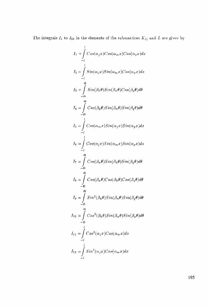
The integrals /; to J34 in the elements of the submatrices i¢;; and L are given by

i

qi = [ Cos(aj2)Cos(amt)Cos(ay)dx

—1

l

I, =/ Sin(a;x)Sin(amt )Cos(Apx )dz

“i e

Is =| Sin(B.8)Sin( B,8)C os( B48 )dé

~@ ©

I, -| C'os( Bp8)Sin(B,0)Sin( B8)dé

-© i

Is =| Cos(amt)Sin(a;x)Sin(apx)dz

~~! I

Ie =/ Cos(aj;z)Sin(amz)Sin(apz)dx

=! ©

Ty -| C'os(Bn8)Sin(3,0)Sin( B08 )dé

-© e

Ig =| Cos(Bn8 )C08( 8,8 )C'0s( 3.9 )d0

-© ©

Ig = / Sin? (B.0)Sin( BrO)Sin( B49 )d0

-O

©

Tyo -| Cos? (B,0)Sin(BnO)Sin(B.0)d0

—o i

Ty -| Cos*(aj;2)Cos(Om2)dx

=! i

The -/ Sin? (a;2)Cos(amx)dx

~I

195

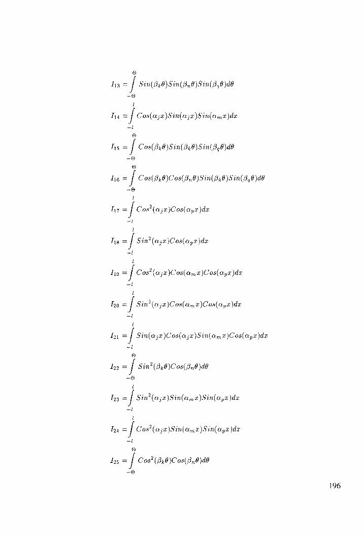
e

3 = / Sin(B,0)Sin(B,0)Sin(340)d0 -©

Tha = [ Cos(aje)Sin(ajer)$in(omda

—l

©

hs = / C0s(8.0)Sin( 8,0) Sin(B,0)d0 -©

oO

Tie -| C'0s( 8,8 )Cos( 8,80) Sin( G8) Sin( 3,6 )de

0 I

Thy? = [ Cos*(ajx)Cos( apt)

—!

l

hie = [ Sin®(as2)Cos(aye)da

-!

i

lig = [ Cos*(aj2)C0s(am2)Cos(ap)de

a I

In = [ Sin? (a2)C'0s(am2)Cos( apd

I

i

In, -/ Sin(a;z)Cos(a;z)Sin(amz)Cos(apz )dz

~! ©

In) = / Sin? (B.0)C0s( 8,0 )d0

-9

Tyg -| Sin? (ajx)Sin(amt)Sin(ap2)dx

=l i

Iy4 =| Cos? (a;x)Sin(am2)Sin(apx)dz

~! 8

To5 -| Cos*(340)C0s(Bn8)d0

-©

196

°

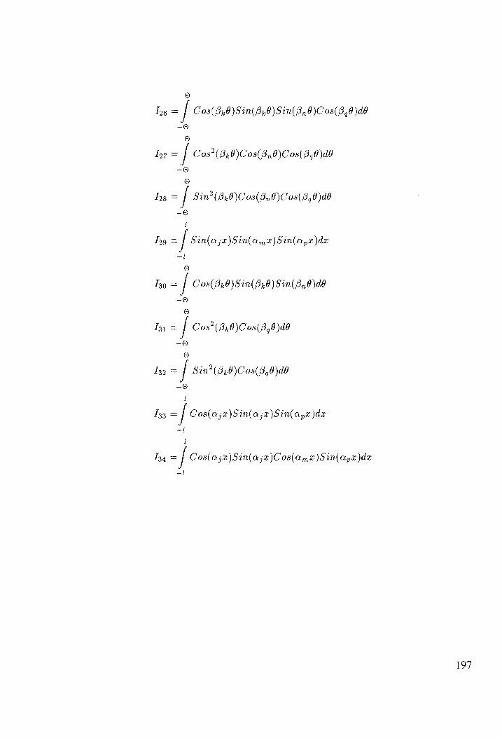
Ig -| Cos(8,8)Sin(B,0)Sin(Bn8)C 08( 8,8 )dé

-9 °

To7 -| Cos? (8,0)Cos(Bn0)C 0s(3,0)d0

-9 3

lhg = / Sin? (B,0)Co0s(Bn0)Cos(B,0)d0

-©

l

Tq -/ Sin(asr)Sin(ams)Sin(apz dz

—i ©

Ix9 = / Cos( Bi,0)Sin(B,0)Sin(Bn0)dd -©

©

I51 = | Cos? (8,0)C0s(3,0)d0 -~©

©

Iz. = / Sin? (B,0)Cos(f,0)d0

-9

I33 -/ Cos(a;xz)Sin(a;z)Sin(apx )dx

-! !

T34 = [ Cos(aje)Sin(aj2)C'os(ame)Sin(aye)dr

—l

197

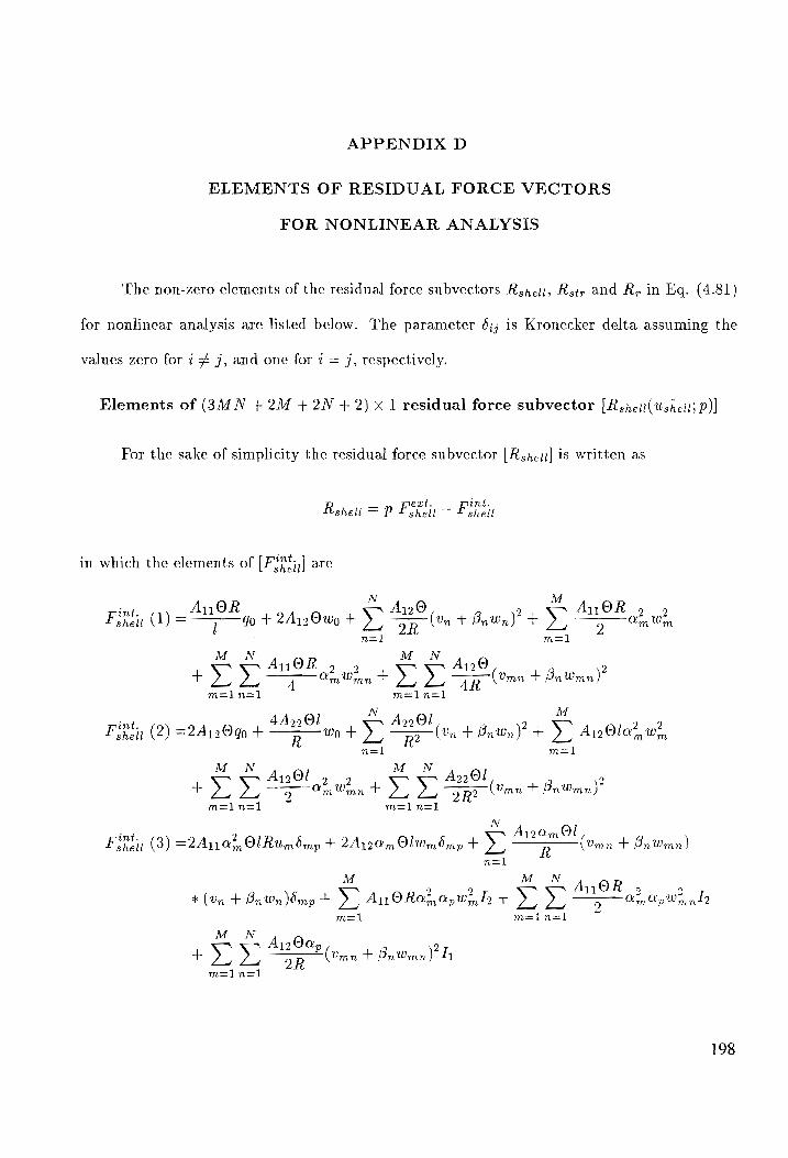
APPENDIX D

ELEMENTS OF RESIDUAL FORCE VECTORS

FOR NONLINEAR ANALYSIS

The non-zero elements of the residual force subvectors Rene, Rsir and R, in Eq. (4.81)

for nonlinear analysis are listed below. The parameter 6;; is Kronecker delta assuming the

values zero for 2 # 7, and one for 2 = j, respectively.

Elements of (3M N + 2M 4+2N +2) x 1 residual force subvector [Repet(ushei; P|

For the sake of simplicity the residual force subvector [Rsp.1] is written as

Rehett = p Fein — Fsheit

in which the elements of (F''"4;,] are

AsiOR A120 Fshe (1) = i w+2An0m +> 4 —

aun aw

M

R (en + BrWn) ? + S-

mal

M WN

Lye Raw ee A120 (a5 + Battmn) m=1n=1 m=1n=1

4A201 A220] Fepent (2) =2A12Oq0 + 3 wo + ya (0m + Brn) + s Ayla? w?,

n=1 mal

N M N 4 S- S- Ah ow a w? > 3 ae" (mn 4 BnWmn)?

A120mOl |

R

F spon (8) =2A110%, Ol Rum bmp + 2A120m Olwm bmp + s n=1

ot 2 9 ae ae 02, 2 * (Un + BnWn)Oomp + S- A119 Raz, apwy le + Ss S| Ap Wynd

mal mrain=l

M oN Array,

+ S- Ss” Vin + BnWmn) i,

m=1n=1

198

Pint, (4) =2A12QmOlUmémp + es a4 Dy 08, )OLRWmébmp + 2A207, OlwoWmémp

1 = 4 2Ass

R + Ay 0%, ORGwWmbmp + yi Ola? (un + Br Wn)? Wmbmp

V\ Age Ol N LR °° AmBn(n + Bn Wn )Umnomp + S- Ao Ola*, (Bron + Wn )Wmn mp

n=l n=l

N Ay Ol M + S° 2 (Un, + Brn \mn + BnWmn)bmp + S- 2A, O R02, aptim Wmls

n=1 ma=1

N M M

— > Age Ola? (Un + BnWn)Vmndmp + S- A110 Ra? apws, 3 + S> Aya n=l mal mal

MN M

Ow? Is + Ss 2A120amapwe, 14 — S- S- AgsOQpOm(Umn + BnWmn)Umnl

m=1 ma=1n=1

Ai +e Om OAp(Vn + Bn Wn )WmUmnl4

A229

2k?

MeN

+ ue m=ln=1

MN Aj 2Age +

+ » »— R. + pp )0amep(Omn + BnWmn) Wmlis + » » m=iln=1 m=1n=1

1

2

A +4 +(Omn + BnWmn) Ly + yas = + 00m Op Bn(Un + Bn Wn)WmWmnls

m=ln=1

M N MeN A 0

+ d dX A12900mOp(BnUmn + Wmn)Wmnla + S- aera . an. w weno

m=1ln=1 m=1n=1

MN M N

+ S° Soi 5A ORO®, ApWmWran lis + > S- AiO R02, apUmnWmnls

mailn=1 m=1n=1

AY Age®

— 2 Bn(Ymn + Brn Wmn)\Umnds

ma=1n=1

n Ago se A22 B? Do Ay Fypen (5) = 2 + ==)? Olvndng + 2(— P + Br, iB 7 Bn Olwnéng + R = 9¢90(0n + Bn

Ai? 2A * Wn)bng + 22 oraa + BnWn)bng + sy as

mal

Om, Ol Umn + Bn Wmn )umo nq

1 (Au 24 M

rk “= ze 7 Ol(vn + Bn Wn We, Ong + S- Ay202, Bn OlwmWmnbn¢

ma=1

A _ > “8 Olam Aetmtlmnd 6ng — -> Age Qla?, WmUmnbng + »4 22 sy Olum

199

Agal Re

Fens, (5) cont'd.

A

= *(Umn + BnWmn ong + > 4 2? sy Ballon + Bn Wn) "Ts + y (Un + Bn Wn)? q;

N 2Aval | M N

a

R?

M N A

+ ) ) [2 lam (Ymn + BnWmn)Umn —~ Ag6QinlOmnWmn + ( A12 | 2A66 — + yl

ma=iln=1 R R R

A Agl «0%, (Up + BnWn)WmWmn _ Bool + om (Umn + BnWmn i Bnimn

+ Wran)| Ls t > yo be 2 (op + BnWn)(Omn + BrWmn) "In + S yi “2 m=1n=1 meine”

+ooe Ja? (tn + BnWn)w,,ls + > s 0.5Ay207 B,lw?, ne

m=1n=1

rin A D A D At: Fin (6) = —_ + + 6,—— a )BnOl Un6ng + (+> 2? Pes Olt + Fp OF nG0( Ban

2A A + Un Jong + oe O1B,wol(Un + BrWn)Ong — s = Ole Om B2Wmtmn6ng

mal

A M 1

+ y Fm Pn Ol Oran + Bn Wmn )Uméd nq — S> Age Ola?, Bn WmUmnOng

m=1

1A 24

+ ae a pe 2 BrOWon + Bntn)w;, bng + 3 A120 OlWm Wmnbn m4 ma=1

A Agal + > Fr Bn Ol0m(Ymn + Bntmn Jing + 7 Fae Bolom + Bun)? tr + »4

n=l

Aol

nant Ez (0m + Bnt0n)?Ty + » 2Aatl gay + Byttn)(Batn + walls + » nel m=ln=

2 Age R

Aggl eS mBnltimnWmn + 3 (mn + BnWmn)(Bn¥mn + Wmn)| Bots

A km (Umn + BnWmn)Umn _ Agea, lumnWmn + (> 2 + Jae lwmWmnlUn

+ BnWn) — R

4 s s 1. PO palo Un + BrWn)(Umn + BnWmn) Ty + S si 1 Au

m=1n=1 motncl

2 Age 2 2 “< 2 2 PR Jar, Bgl(tn + BnWn)Wmnts + S° Ss" 0.5A;207, lw, te m=zln=1

+

200

Figtn (1) = [(Ano}, + 82 a = QI Rumn + (A12 + Ase )OmSnOl¥mn + A120m OlWmn

Abe _ me + Bn Wn)Wm| Smpbng + > mln + BnWn)(Umn + Bn

A A *Wmn)Ompl3 — sf —— Am Bgl (Un + BnWn)Wmnbmpls — s = am Sn®

R R n=1 m=1

M MN A 12 +(Omn + BnWmn)mSngls + x Ay1 02, GpORWmWmndngl2 + iu dX oR

N Age

*O p(Umn + Bn Wmn) * TT. _ s LL > AmBg(Umn + BnWmn)Wmnlals marl

M N

+ S° $0 05An 07, opRw;, Lele mazln=l

Aga +=8 R

42 (Dy. + 2Dé6)

PER (8) = {(Arz + Abe)ambnOltmn + (E+ 5262 + (os + 22 )02, R] Olvyn A D A 7 + ape bcm + (amt — Agea2, Wm t R R

A Q. “< As

+ Rr Wm )(n + Bn Wn )Ol + ( v do + or lwo )(Umn + Bnwmn)® | mpSng

N A Aol

+2 (FG Su — AggQmWmn )lom(Un + BnWn) + a [( + 82 )(Wnmn

A +UnWmn) + 28n(UnUmn + WnWmn)| \ bmpls + > e 27 8 Bgl(vn + BnWn)

1. 4 * (Umn + BnWmn)ompl3 + yb 2? I(v Un + BnWn)° (Umn + BnWmn)ompl7

n=l

A A M

+ yr(ae ~ QmUm + ae m)(Umn + BnWmn)Obngli + S° | 41202, Bn tm

mal m1

1A 2A A + 5 zr + Re QW Wm (Un + BnWn) _ Agee, Umn _ > Om Bntimn| Owmobngdl2

M M 1 (fiz 1 oe

+ 2 3 5 RR Ja‘, 2 O( (Omn + BnWmn)w, bnglit _ Xu AgeQmOpO(Umn

MN Ags

+BnWmn)Wmbn¢ql4 + Xu » [2 am tim + R? —(BnUmn + wmn)| (Umn

201

Feheit (8) 0.522 1 5An cont'd. 7 = + Bn mn) Is + S yo OSs g(Umn + BnWmn) Is + s ye

m=ln=1 m=i1n=1

we 5A +(Un + BnWn)(Umn + BnWmny Lily + y y a Umn + BnWmn) Int

m=l1n=1

M WN A 2A A

+ S° S° (+ > Jaz, (vn + ByWn)Wm — Ag6Q?, mn _ > Om Bntmn|

m=1n=1

M WN

*Wmndots + s s 0.5Ay207, B,w2,nlole — S- > Ag6QmOpSn Winn tals m=1n=1 m=ln=1

MN 1,A 2A

+ » » (> 2 Jorn (Yn + Bn Wn Winn to Ts m=1n=1

MeN A 2A

+ S| > z a2, (Umn + BnWmn)WmUmnlshii

m=l1n=1

M WN 1,Ay2 , 2Ag6e

+ , > ap + > Jaz, (Omn + BnWmn)Wmntshi m=1n=1

in A , D Di. +2D Pern (9) = { A120 lttmn + = + Bue = + a7, Ow t Pes) BnlUmn

Ad D Dio + xD 0.5A

+ | + a8 mt? 2 = R 9 + Dya%, R) bmn + (—— i a9

Agog R2 \Omn + BaWmn) Bn + (0.5A1190R + Ay wol)a2, Wmn

A A22 + (Fem tm + R2 = Wm (Op + BrWn)Bnl + A2Q%, U(Bnn + Wn) | O8rmpbn

N A

“DA 66Q2, (un + Ba Wn )0mntsbomp — > pom Brl(tm + Bun )ttmndsbmp

n=1 n=l

N +> {= Aggl

—~ Om Umnl Un + BnWn) + [(1 + B2)(Wndmn + UnWmn) + 2Bn Re

' +(UnUmn + WnWmn)| \ G41 mpls + S au (Un + BnWn)(Umn + BnWmn)ompl3

n=l

1. ~* ' + > ae —3— (vn + Brin) (Umn + BnWmn)Bqompl7 + s A120%, lWmn(Bntn

n=1

1 (4 1 24 1 (4 +wn)Omple + vi > 70 2 “lun + Bn Wn)? Wmbmpl3 + ar ou

202

Fen (9) _ 4-8 2 At cont'd. em l(On + Bn Wn) WmnOmpliz + Xu Pp OPO tim (mn + BrWmn)bng

* iy + Ss" | A120’, Wmn + aR R p 2 BnWm(Un + BnWn) — Agee, BnYmn

m—o1

M A — Sam Si timn | Owmbngl2 + Y> A1290mOp(Bnmn + 2Wmn)Win bugle

m=1

“A + US 2? sy BnOwm(%mn + BnWmnyongli + s 1. 5A110Ra?, Ap We, Wmnbngli3

m=1 m=1

“1, Ap 2A M 66

+ S- 5(G t+ Ja , mPnO(Vmn + BnWmn)Way 6ngfi1 + S- A119 Ra?, Ap

m=l1 m=1

*( Wm tmn + Um Wmn)ongla + s s [= AmUmn + 2 (BnUmn + Wmn)| (Vmn

m=1n=1

1. 4 + BnWmn) Bah ts + s S A12AmOp(BnUmn + Wmn)Wmndlale + s yi 2

m=l1n=1 m=l1n=1

0. oa «(Un + BnWn)(Omn + BnWmn) Balilz + s yo (Umn + BnWmn) Bolte

m=1n=1

M N A 2A 9 A

+ X a ( > + 2 a? (Un + Bn Wn )Wm _ AgeQy,Umn _ > Om Bn tm

M N

*BqgWmntols + S- Ss” 1.5A1103,0,Rumwe ples + s s 0. 5Aya w? ole

m=iln=1 ma=tn=1

M N 0.5A M WN

+ pr mn + Bam) lls + D7 D050 Op RW nn lishs m=ln=1 m=l1n=1

MN A

+ S- S° Ay0%, An RUmnWmntlale _ s 7 po Ba(Omn + BnWmn)Umntst4

m=1n=1 m=l1n=1

M N A 2A MN

+ S| (= t+ .e Rom (Umn + BnWmn)WmUmnbelsfhii _ S- S- Ag6Qm Op

m=iIn=1 m=1n=1

M N J (4 2A

*(Umn + BnWmn)Umntl3t4 + x 2d 3 (= + =e 2 ‘(tn + Bn Wn We» Bqlots

MN A

+ » ye + “es )Om Ap (Un + BnWn)(Umn + Brn Wmn)WmIal4

Hi —_

ma=in

203

Fh (9) cont'd,

1 A . 2466 2 _ +s. S~ (pe 4 pam ep(Mrnn + BnWmn)” WmIshs m=a1n=l

MN A 2A

+ > S-( —" + ae Om Ap( Un + BnWn)(Umn + BnWmn)Wmnlah7

m=1n=1 R R

MN 1A 2A

+ S| S- (> + > Om Ap(Umn + BnWmn)” Wmnlish7

m=i1n=1

A

MX 2A 12 66

+ » » ap + R )\(Omn + Bn Wmn JO, W w? nBalelii,

and the elements of [F'°';,] are given by

M N N

Fest. 2 1 2 1 2 2 Fshell (1) =(R wo) O+ D3 0un + 2 ZO + we) + D/ OBntnton

M WN

O(Vmn tmnt >, > m=1 n=1

OP BnUmnWmn

ho] re

Mes

Me

Fert, (2) =4(B + wo)Ol + 2(R + wo)Oqo + y 20m Oltim Wm + s s Am OlUmnWmn m=ln=1

Feeil (3 ) =2(R + Wo )Om OlwWm bmp + > arOw? ti + y Amn Ol(vy, + Bn Wn )VmnOmp

m=l1 n=1

N

+ » Am Ol Brn + Wn )\Wmnd mp + s yo! 329 Vn + wen)

=1 mazln=l

M WN 2

+ » 3 SAmPnOVmnWmnls + s x2 5 OpPnOUmnWmnlt

m1? mot nai > any mr

M

PEE) (4) =2(R + Wo )omOltm bmp + (21 + Go)OWmSmp + YD 20m OUm Wms m=1

M N

+ Am Ol Bnvn + Wn )UmnOmp + S| S- Om OUmnWmnlt

m=1n=1 3 i han

n [Om (1 - Iz) + 2ap14|Umnmn

ele

ive

204

MN

Frei (5) =(2l + qo)(Un + Bn Wn )Obng + s Am OlBnWmUmnOn ng S- > OmlUmnUmnds

ma=1 ma=i1n=1

+ s AmnmOl(omn + BnWmn)Umong + s x? ~Aml( (B,L5 + Bole )UmnWmn

m=1 mataci?

M

FSReil (6) =(2/ + Go (Bn Vn + Wn )Obng + > Am OlWmUmnong

m=l1

M N

AmOl(Brvmn + Wmn )tmong + S- S> OmlumnWmnte

m=1n=1

N

+

Me

3 UL

+ aml [Bn (Te — Is) + 26,15] UmnUmn

Cpr

Mes

ma=1n=1

Fei (7) =(R + w Wo )OmOlWmndmpong + (nvm + Wn Am Olwm bmpbng

M

+ Ss" ApOWmWmnl6 ng t aE «8,0 (ma + Aaph )WmUmnbn nq

m=1 m= 13

N

+ S| AmlWnWmntedmp + aE ~ ml Bute — Bqls)Wn¥mnbmp

n=1

N

+ S- AmlUnVmntsé6 mp + y? —Qm nl (WnUmnls + UnWmnle)imp

n=1 n= 13

N 1 + 223 © ermal Bn Es + Bats )UnWmnd mp + > s 5 eel v2 nts + we, nie) hi

m=in-1

+ s yo! * Bal Om Ls + Andy )(Is + Ig )0mnWmn

m=1n=1

Frei (8) =(Un + Bn Wn )OmOlumbmpbng + (Umn + BnWmn)Olbmpbng

N

+ 59(%mn + BnWmn)qo5mpong + >, OmlUntimntsdmp n=1

+ s AmOUmUmntibnq + x2 8, ( cm Ia + Ans )UmWmnbn ng

m=1 mat?

+ x2 = cmBn@ Wry ttimn 126g + rE * g,0(OmLs _ pls )WmUmnon nq

m= 3

N

+ y3 2 mBnO tn Wranlibn +) > 5a ml Bnls + Bqle)Wntmndm mp

wee

n=1

N MeN

> S| AmUmn’mntils + Ss” S>

ma=1n=1 ma=1n=1

am(BnIs + Bole )(h + In )tmnWmn

eo

[|

205

Fereil 3) =(BnUn + Wn )Om OlUmbmpbng + (Bnmn + Wmn)Oldmpong

1 + 5 OBn?mn + Wmn)doompong + (R + Wo )QmOlUmnbmpbng

M M 1

+ by Am OUmWmntlibng + S- ghnr9(Omle + Ans )UmUmnOnq

m=1 m=1

M N 2 1

+ S- 53m Pn Olin Vmnti ong + Ss" goml(Bnds + Bals)UnUmnOmp

m=1 n=l

M N N 2

m= n=1 n=1

N

+ S| AmUmnWmnlile

r=

»

Mes

M=

Me

3 fl _ 3 u 3 {! ee

Br(Omd2 + Only \tmnUmnds3 +

bn

Am Bg (hh + In )UmnUmnds Me

M4

Mes

3 I 3 W 3 u 3

Brlamhy + Apls )UmnUmnle +

ee

Elements of (2M +1) x1 residual force subvector [R,:,(ws:,)]

M

(EA) Rsir (1) =n 4 x 0.25(EA),a2, wn

M

Reir (2) =(EA) 07, !tembmp + > _ 0.5( EA) 05, Up Wom 2 m=1

M Retr (3) =[0.5(EA) sq + (ED) .07, 102, wemébmp + s° 0.5(£ A),03, apwe, tis

m=1

M

+ S° (EA),07,QpUsmWsmla

m=1

206

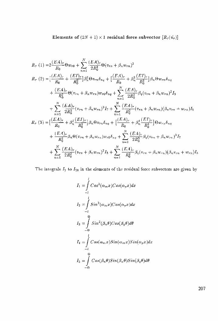
Elements of (2N +1) x 1 residual force subvector [R,(1-,)]

R, (1) = =2 Ow Wr0 +> SHE O(n + Brien)

R, (2) =(— + teat Urn Ong + 7 + Zs : "| BnOWrndng

EA), EA), + ( © O(Urn + BnWrn)Wrobng + » EA + BnWrn) Ts

(BA (E a >? mS =(Urn + BnWrn) “Tr + » (v Ven + Bn Wen )(Bnven + Wrn) ds

R, (3) = Ay + BF oe "| Bn Ovrnbng + te + (BF Fe Owenbn 2

(EA), ae + Re BnO(vrn + BnWrn) )wrodn +yS Balen + Bn Wrn PL 7

N vo. (EA), + d 2R? (Urn + BnWrn)? b+

by

Jn g ( Urn + Bn Wen (Bren + Wen )ds

The integrals £; to dig in the elements of the residual force subvectors are given by

i = [ Cos*(ams)Cos(apsr)de

D) =/ Sin? (Qm2)Co0s(apx)dx

©

Ts =| Sin? (Bn0\C os( 8 0)de

-9 l

Ig =/ Cos(mt)Sin(amt)Sin( aps dz

-l

Is -| C'os( BnO)Sin( Bn8)Sin(B,6)dé

-9

207

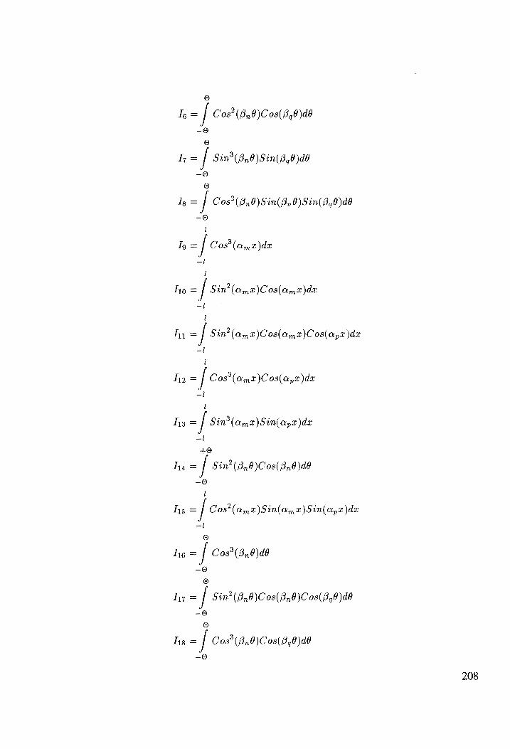
8

Ig = / Cos? (Bn0)C 0s( 8,0 )d0

©

In= / Sin? (Bn9)Sin( 8,0 )d6

Ig = / C0s*(Bn8)Sin(Bn0)Sin(B0)d0 -©

i

Ig = [ C0s° ams)

—l

l

Tio = [ Sin®(amt)Cos(am)da

Ty -/ Sin? (Qm2)C 0s(Amt)Cos(apx)dz

=I

Tho = [ C08°(4m)Cos( apd

=]

Tig -/ Sin? (Qm2)Sin(apx)dz

—I +0

Tg = / Sin? (Bn0)C0s( BnO)db -©

i

Ths =/ C0s* (Qm2)Sin(Amt)Sin( apyx)dz

-! ©

le = / Cos?(B,0)d0 —-O

0

Iz -| Sin? (BnO)C0s(Bn9)C 0s(3,0)d0

-© ©

Tig =| Cos*(Bn9)C 0s(840)d0

-e

208

VITA

The author was born at Delhi in India on February 21, 1963. He completed his

elementary and secondary education in Delhi, and received his Senior Secondary

Certificate from Government Model school, Civil Lines, Delhi in 1979. He obtained

his B. 5. degree in Aerospace Engineering from Panjab University, Chandigarh

in 1983, and joined Hindustan Aeronautics Limited as a Design Engineer. He

was sponsored by the company to pursue graduate studies at Indian Institute of

Technology, Madras, and he was awarded a Master degree in Aerospace Engineering

in 1987. He received on-the-job training at M/s Dornier Aircraft Limited, Germany,

on the manufacture and quality assurance of Dornier Do-228 composite parts. He

served Hindustan Aeronautics Limited in various capacities for eight years and

resigned as Deputy Manager in August, 1991 to come to the United States in

pursuit of higher education. In Fall of 1992, he was accepted to the Ph.D. program

in Aerospace Engineering at Virginia Polytechnic Institute and State University.

ee Naveen Rastogi

VITA 209

APPROVED: Cue Kh Soler - VTechWorks

Documents

Transcript of APPROVED: Cue Kh Soler - VTechWorks