Fluid Film Bearing Test Rig - VTechWorks

Evaluation of the VPI & SU Fluid Film Bearing Test Rig

by

Erik Evan Swanson

Thesis submitted to the Faculty of

Virginia Polytechnic Institute and State University

in partial fulfillment of the requirements for the degree of

MASTER OF SCIENCE

in

Mechanical Engineering

APPROVED: ot] R.G. Kirk, Chairman

F.J. Pierce R.H. Plaut

March, 1992

Blacksburg, Virginia

LO Suss yess VA 2.

S418

Evaluation of the VPI & SU

Fluid Film Bearing Test Rig

by

Erik Evan Swanson

Chairman: R.G. Kirk

Department of Mechanical Engineering

(ABSTRACT)

The design of advanced, state-of-the-art turbomachinery requires accurate analytical tools for

predicting rotor response and evaluating stability. One of the required tools is a reliable

analytical code for predicting the performance of fluid-film bearings. This work presents an

initial evaluation of a test rig for verifying such codes. This presentation includes

background information on the techniques and terminology of fluid-film bearing analysis and

two basic approaches to experimental evaluation of fluid-film bearings. To establish one

such code, NPADVT, as a useful tool for evaluating the performance of the test rig,

comparisons between six published, experimental evaluations of fluid-film bearings for static

characteristics and the corresponding NPADVT analysis are presented. With the code thus

anchored, and its limits established, experimental data generated with the test rig are

compared to appropriate analyses and the test rig shown to be essentially functional. Finally,

experimental static results for a pocket bearing generated with the test rig are presented and

compared with analysis.

Acknowledgements:

I would like to acknowledge the support of my parents and thank them for giving me an

innate curiosity about the world that has made this thesis possible.

I would also like to thank Dr. Kirk for his support and assistance with this work,

John Nicholas of Rotating Machinery Technology for supplying the test bearing, Ingersoll-

Rand/Torrington for donating the test rig and NASA Marshall for granting me a Graduate

Research Fellowship.

In addition, I would also like to thank the many outstanding teachers I have had the

privilege of learning from throughout my formal education. Finally, I would like to thank

the "working men" in the maintenance department of the Stone Container - Hopewell

papermill with whom I worked as an undergraduate while in the Co-Op program. Without

some of the skills they taught me, I would never have been able to complete the experimental

portion of this work.

Erik Swanson

Blacksburg, Virginia

March 14, 1992

Acknowledgements lil

Table of Contents

Chapter 1

Introduction and Literature Review ....... 0... cee eee ee ee ee ee eee 1

1.1 Purpose and Scope of Work ........... 000 ee eee eee eee ee eee 1

1.2 Approaches to Fluid-Film Bearing Analysis .................24.- 5

1.2.1 Fluid-Film Bearing Geometry Definitions ................. 6

1.2.2 The Reynolds Equation .......... 2.0.00. eee eee eee 9

1.2.3 Computer Based Solutions ................. 200+ ees 10

1.3 Bearing Analysis With Code NPADVT .................--2-0-0-- 16

1.4 Published Results for Axial-Groove Bearings .................--. 21

1.5 Published Results for Pocket Bearings ................-.-22-0-00045 23

Chapter 2

Experimental Approach... 0... cc ee ee eee 24

2.1 Approaches to Test Rig Design .......... 0... cee eee eee ee eee 24

2.2 Floating Bearing Rigs... .. 2... 0.2... eee ee ee ees 26

2.2.1 Advantages to Floating Bearing Paradigm ................. 27

2.2.2 Disadvantages to the Floating Bearing Paradigm ............. 28

2.3 Dual Rigid Bearing Mounts ........... 0... 2 eee eee ee ee ee ee 31

iV

2.4 Rigid Mount, Single Test Bearing ..............2.0 02s ee eeees 32

2.4.1 Advantages to Rigid Bearing Paradigm .................. 32

2.4.2 Concerns with Rigid Bearing Paradigm .................. 33

Chapter 3

Comparisons: NPADVT vs. Published Experimental Results .................. 36

3.1 Overview 2... ee ee 36

3.2 Comparison for Tonnesen/Hansen ...........-.. 0.0. ee eee eee 39

3.2.1 Data 2... eens 39

3.2.2 Discussion of Results ..... 2.2... 0.2.2... eee ee ee ee 48

3.3 Comparison for Lund/Tonnesen ........ 2.0.00. eee eee eee ene 49

3.3.1 Data... ee ne 50

3.3.2 Discussion of Results ... 2.2.2... 2.0.02. cee eee ee eee 60

3.4 Comparison for Someya #2 2.2... .. ee es 60

3.4.1 Data... eee 61

3.4.2 Discussion of Results ............ 2.0002. eee ee eee 71

3.5 Comparison for Someya #3 ... 2... 2.0... eee ee ee eee 72

3.5.1 Data... ee ee 72

3.5.2 Discussion of Results ......... 2... 0.02... eee eee ee eee 79

3.6 Comparison for Someya #5 2.1... . ee ee ees 79

3.6.1 Data... ee ee 80

Table of Contents Vv

3.6.2 Discussion of Results ............ 0000 ee eee eee ee eee 83

3.7 Comparison for Andrisano .. 2... 2.2... ee ee ee ee ee ee ne 83

3.7.1 Data... ee ee eee 84

3.7.2 Discussion of Results ...... 0.0... 0. ee ee ee es 92

Chapter 4

VPI & SU Test Rig... 2. ee ee 94

4.1 Introduction and Orientation... 2... 2... 2... 2.02.2 eee ee eee ee 94

4.2 Rig History ... 2... es 95

4.2.1 Summary of Test Rig Capabilities ..................... 98

4.3 Detailed Description of Test Rig 2.2... 0. ee ns 99

4.3.1 Mechanical Details ..... 2... . ee ee 99

4.3.2 Magnetic Loading System ................2.00 002 ee 103

4.3.3 Air Turbine Drive ......... 0.0... ee eee ee eee 106

4.3.4 Test Bearing Oil System... 2... ee ee 107

4.3.5 Other Instrumentation ................-02.-02 22 ee eee 108

4.4 Sensor Calibration... 2.2... ee ee 110

4.5 Uncertainty Analysis ......... 0.0.02 ee ee eee 115

4.5.1 Discussion of Approach Employed ...............2004. 115

4.5.2 Zeroth Order Error Analysis ...............2-0202000- 118

4.5.3 Sensitivity Analysis ......... 0.002 eee eee ee ee ee 126

Table of Contents vi

4.5.4 First Order Analysis .......... 0.0... 20. eee eee ee eee 135

4.5.5 N™ Order Analysis... 0... ee ne 137

Chapter 5

VPI Experimental Results and Comparisons for a Two-Axial-Groove Bearing ...... 139

5.1 Introduction... 2... ee eee 139

5.2 VPI & SU Test Bearing and Oil... 2... ee ee ee 140

5.3 Experimental Procedure .............- 2.0.2 eee eee ee eee ee 142

5.4 Experimental Two-Axial-Groove Data........... 0.2002 eee eee 145

5.4.1 Data... eee 145

5.4.2 Discussion of Results ........0.. 0... 0. 154

5.5 Comparisons Between Experimental Results .................-4. 155

5.5.1 Repeated Test Comparisons .............. 2.000 e eee 156

5.5.2 Discussion of Repeated Tests .......... 0.0. cee ee eee 161

5.5.3 Removal/Reinstallation Repeatability ................... 162

5.5.4 Discussion for Removal/Reinstallation Comparison .......... 164

5.5.5 Comparisons for Variable Feed Pressure ................ 164

5.5.6 Discussion for Feed Pressure Comparisons ............... 167

5.5.7 Comparisons between NPADVT and VPI Data ............ 168

5.5.8 Discussion for Comparisons to NPADVT ................ 186

5.6 Comments and Discussion ..... 2... 0... 000 eee ee ee ees 188

Table of Contents Vii

Chapter 6

VPI Results and Comparisons for Pocket Bearing .................-.0200% 192

6.1 Introduction... 2... ee ee 192

6.2 Pocket Bearing and Oil... 2... ee ee ee 193

6.3 Experimental Procedure .... 2... 0... eee et ee ns 195

6.4 Experimental Pocket Bearing Data and Comparisons ............... 196

6.4.1 Data... ee ee 196

6.4.2 Discussion of Results .......... 0.2.2.0. eee eee eee 200

6.4.3 Comparisons For Repeated Tests ............ 0000220 201

6.4.4 Discussion of Repeated Tests ................2 0000 205

6.4.5 Comparisons Between NPADVT and VPI for Pocket Bearing... . 206

6.4.6 Discussion of NPADVT vs. VPI for Pocket Bearing ......... 217

6.4.7 Comparison Between Pocket and Plain Bearing ............ 218

6.4.8 Comments on Bearing Type Comparison ................ 220

6.4.9 Comments and Discussion for Pocket Bearing ............. 221

Chapter 7

Conclusions and Recommendations ..........-.....0- 2 eee eee eee eee 223

7.1 Conclusions for NPADVT .......... 00.0. eee eee ee een 223

7.2 Conclusions for the VPI & SU Test Rig ....................6.. 224

Table of Contents Vili

7.3 Recommendations for NPADVT ................02. 00000 ee ae 225

7.4 Recommendations for Test Rig .......... 2.20 eee ee eee ees 227

7.4.1 Thermal Growth Effects ................-02. 0002007 228

7.4.2 Other Misalignment Effects ...............2.0022008. 230

7.4.3 Data Acquisition .. 2... . . ce 231

7.4.4 Oil System... 2 2 ee ee 234

7.4.5 Speed Control... 1... es 235

7.4.6 Miscellaneous Instrumentation Upgrades................. 237

7.4.7 Rig Mechanical ... 2... 2... ee ee 238

7.4.8 Miscellaneous Recommendations ................20005 240

7.4.9 Priorities... es 242

References 2... ee ee ens 247

Appendix A... ee 250

Appendix B... ee eee 254

B.1 Confidence Areas .. 21... ene 254

B.2 Analysis of Variance Output ... 20... 2... 2 eee ee eee 257

B.3 Sample Uncertainty Calculations ........... 0.0.00. eee ee eee 259

B.3.1Sample Calculation #1 - Bearing Centerline Estimation ........ 259

B.3.2 Sample Calculation #2 - Estimation of Number of Samples ..... 260

Vita Le ee 263

Table of Contents 1X

Fig.

Fig.

Fig.

Fig.

Fig.

Fig.

Fig.

Fig.

Fig.

Fig.

Fig.

Fig.

Fig.

Fig.

Fig.

Fig.

Fig.

Fig.

Fig.

Fig.

List of Figures

1: Two-Axial-Groove Bearing Geometry ............ 2.2.00 epee eee eee 7

2: Additional Geometry for Pocket Bearing ........... 0.000 e cents 7

3: Fluid-Film Bearing Geometric Parameter Definitions .................. 8

4: Fluid-Film Analysis Geometry ....... 0... 0. 0c eee eee eee eee eee 8

5: Typical NPADVT Grid .. 2.2... ee ee 19

6: NPADVT Flowchart ..... 20... .... ee eee ee eee 20

7: Floating Bearing/Fixed Shaft Test Rig ..........0. 0.002. eee eee 25

8: Floating Shaft/Fixed Bearing Test Rig... ....... 0... 0.2... 25

9: X-Eccentricity Ratio for Tonnesen, 6.67 Hz ............-...-.2-0-2 08-5 42

10: Y-Eccentricity Ratio for Tonnesen, 6.67 Hz ................--.+--5 42

11: X-Eccentricity Ratio for Tonnesen, 26.67 Hz ................-25055 43

12: Y-Eccentricity Ratio for Tonnesen, 26.67 Hz ...............-2---0-- 43

13: X-Eccentricity Ratio for Tonnesen, 80 Hz..................-0008- 44

14: Y-Eccentricity Ratio for Tonnesen, 80 Hz............. 02.002 ee eee 44

15: X-Eccentricity Ratio for Tonnesen, 133.3 Hz................--.-.-.. 45

16: Y-Eccentricity Ratio for Tonnesen, 133.3 Hz..................2-6-. 45

17: Percent Error for Tonnesen, 6.67 Hz.............. 00002 ee ues 46

18: Percent Error for Tonnesen, 26.67 Hz .......... 0.0... e eee eee 46

19: Percent Error for Tonnesen, 80 Hz ........... 0.002. eee eens 47

20: Percent Error for Tonnesen, 133.33 Hz ..........0.0 0... 2.00 eee eens 47

Table of Contents x

Fig.

Fig.

Fig.

Fig.

Fig.

Fig.

Fig.

Fig.

Fig.

Fig.

Fig.

Fig.

Fig.

Fig.

Fig.

Fig.

Fig.

Fig.

Fig.

Fig.

Fig.

Fig.

21:

22:

23:

24:

25:

26:

27:

29:

30:

31:

32:

33:

34:

35:

36:

37:

38:

39:

40:

41:

42:

X-Eccentricity Ratio for Lund, 33.33 Hz ............ 2.02.2 eee eee 52

Y-Eccentricity Ratio for Lund, 33.33 Hz ............... 00020028 52

X-Eccentricity Ratio for Lund, 58.33 Hz .................22..-00- 53

Y-Eccentricity Ratio for Lund, 58.33 Hz ...............-2. 000000. 53

X-Eccentricity Ratio for Lund, 83.33 Hz ............... 20200000 54

Y-Eccentricity Ratio for Lund, 83.33 Hz .............-...02.0 020 es 54

X-eccentricity for Lund, 108.33 Hz... . 2... 2. ee ee ee ee es 55

: Y-eccentricity for Lund, 108.33 Hz............. 2.02. .0 022.0. 55

Percent error for Lund, 33.33 Hz (Stationary Probes) ................ 56

Percent error for Lund, 33.33 Hz (Rotating Probes) ................. 56







X-Eccentricity Ratio for Someya Test 2,50 Hz ...............-.-.. 63

Y-Eccentricity Ratio for Someya Test 2,50 Hz .................... 63

X-Eccentricity Ratio for Someya Test 2, 10OOHz.................... 64

Y-Eccentricity Ratio for Someya Test 2, 100 Hz.................... 64

X-Eccentricity Ratio for Someya Test 2, 150 Hz.................0.. 65

Y-Eccentricity Ratio for Someya Test 2, 150 Hz.................00. 65

List of Figures Xl

Fig.

Fig.

Fig.

Fig.

Fig.

Fig.

Fig.

Fig.

Fig.

Fig.

Fig.

Fig.

Fig.

Fig.

Fig.

Fig.

Fig.

Fig.

Fig.

Fig.

Fig.

Fig.

43:

45:

46:

47:

48:

49:

50:

51:

52:

53:

54:

55:

56:

57:

58:

59:

60:

61:

62:

63:

64:

X-Eccentricity Ratio for Someya Test 2, 200 Hz.................... 66

: Y-Eccentricity Ratio for Someya Test 2, 200 Hz.................... 66

X-Eccentricity Ratio for Someya Test 2, 250 Hz..............-....-.. 67

Y - Eccentricity Ratio for Someya Test 2, 250 Hz.................4.. 67

Percent Error for Someya Test 2,50 Hz ...............-.-222.22-- 68

Percent Error for Someya Test 2, 100 Hz... 2... 0... .. 02.0000 ee eens 68

Percent Error for Someya Test 2, 150 Hz .................2.2.0000- 69

Percent Error for Someya Test 2, 200 Hz ..............-.-2-.2-02006- 69

Percent Error for Someya Test 2, 250 Hz .................2.20-4.- 70

X-Eccentricity Ratio for Someya Test 3, 26.7 Hz .............-...--. 74

Y-Eccentricity Ratio for Someya Test 3, 26.7 Hz .................-.. 74

X-Eccentricity Ratio for Someya Test 3, 66.7 Hz ................4.. 75

Y-Eccentricity Ratio for Someya Test 3, 66.7 Hz ................2-4.- 75

X-Eccentricity Ratio for Someya Test 3, 100 Hz.................... 76

Y-Eccentricity Ratio for Someya Test 3, 100 Hz.................... 76

Percent Error for Someya Test 3, 26.7 Hz ............2.. 02000 eee 77

Percent Error for Someya Test 3, 66.7 Hz ............ 2.000202 eee 77

Percent Error for Someya Test 3, 100 Hz .......................4. 78

X-Eccentricity Ratio for Someya Test5 ..............--2.-.00 0006} 81

Y-Eccentricity Ratio for Someya Test5 ..............22. 020-2000. 81

Percent Error for Someya Test5 ............2. 02.002 ee eee ee eee 82

X-Eccentricity Ratio for Andrisano, 10 Hz .....................-.. 86

List of Figures xii

Fig.

Fig.

Fig.

Fig.

Fig.

Fig.

Fig.

Fig.

Fig.

Fig.

Fig.

Fig.

Fig.

Fig.

Fig.

Fig.

Fig.

Fig.

Fig.

Fig.

Fig.

Fig.

65:

66:

67:

68:

69:

70:

71:

72:

73:

74:

75:

78:

79:

80:

81:

82:

83:

84:

85:

86:

Y-Eccentricity Ratio for Andrisano,10 Hz... 1.2.2... 2.2.2... 2.0. ee eee 86

X-Eccentricity Ratio for Andrisano, 20 Hz ............-.----2200-. 87

Y-Eccentricity Ratio for Andrisano, 20 Hz .............---.--0-2004- 87

X-Eccentricity Ratio for Andrisano, 30 Hz ................-..-20-. 88

Y-Eccentricity Ratio for Andrisano, 30 Hz ...........-.-..-.-220--. 88

X-Eccentricity Ratio for Andrisano, 40 Hz .............-..-.-2-000. 89

Y-Eccentricity Ratio for Andrisano, 40 Hz ...............2022000- 89

Percent Error for Andrisano, 10 Hz ................20 0000000006 90

Percent Error for Andrisano, 20 Hz ............0 2... 00.00. ee eee ae 90

Percent Error for Andrisano, 30 Hz .............. 2.00000 eevee uae 91

Percent Error for Andrisano, 40 Hz .............0.. 2.2.00. 00 00004 91

: VPI & SU Fluid Film Bearing Test Rig .........2....-22.220-2006. 96

: Test Rig Sketch... 2... ee ee 97

Shaft/Magnet Arrangement ..... 2... 2... 0 eee eee ee eee eee 105

Uncertainty Analysis Geometry ............ 0.0.02. ee eee eee 120

Percent X-Eccentricity Ratio Change per Hz ..............2-20200- 127

Percent Y-Eccentricity Ratio Change per Hz ..............-2.2-4-. 127

Absolute Shaft X Position Change (mm) per Hz ................... 128

Absolute Shaft Y Position Change (mm) per Hz ................... 128

Percent X-Eccentricity Change per DegreeC .................-..-.. 129

Percent Y-Eccentricity Change per DegreeC ........-.........004. 129

Absolute Shaft X Position (mm) Change per Degree C ............... 130

List of Figures Xlil

Fig.

Fig.

Fig.

Fig.

Fig.

Fig.

Fig.

Fig.

Fig.

Fig.

Fig.

Fig.

Fig.

Fig.

Fig.

Fig.

Fig.

Fig.

Fig.

Fig.

Fig.

Fig.

87:

88:

89:

91:

92:

93:

94:

95:

96:

97:

98:

99:

100:

101:

102:

103:

104:

105:

106:

107:

108:

Absolute Shaft Y Position (mm) Change per Degree C ............... 130

Percent X-Eccentricity Ratio Change per N load .............-..... 131

Percent Y-Eccentricity Change per N Load ....................-.. 131

: Absolute Shaft Position (mm) Change per N Load .................. 132

Absolute Shaft Position (mm) Change per N Load .................. 132

First 16.7 Hz Test (Cd = 0.15 mm) ..... 2... ee ee ee ee 147

First 33.3 Hz Test (Cd = 0.148 mm) ..... 20... 0... 02. ee eee eens 147

First 58.3 Hz Test (Cd = 0.146mm) ....................0.00. 148

First 83.3 Hz Test (Cd = 0.158) 2... ee ee 148

Second 16.7 Hz Test (Cd = 0.156 mm) ....................006- 149

Second 33.3 Hz Test (Cd = 0.152 mm)..................020005 149

Second 58.3 Hz Test (Cd = 0.149 mm) ....................008. 150

Second 83.3 Hz Test (Cd = 0.148 mm) ...................200-. 150

33.3 Hz, 0.069 MPa Test (Cd = 0.154 mm) ................... 151

33.33 Hz, 0.137 MPa Test (Cd = 0.154 mm) ................... 151

33.3 Hz, 0.172 MPa Test (Cd = 0.153 mm) .................... 152

33.33 Hz Test after removal/reinstallation (Cd = 0.149 mm) .......... 152

83.3 Hz Test, after removal/reinstallation (initial Cd = 0.149 used) ...... 153

16.7 Hz Repeated Tests - Actual Data ............-..-.-2..02004 157

16.7 Hz Repeated Tests - Normalized Data ..................4-. 157

33.3 Hz Repeated Tests - Actual Data ...........-..-.--...2.2-- 158

33.3 Hz Repeated Tests - Normalized Data ...................-. 158

List of Figures XIV

Fig.

Fig.

Fig.

Fig.

Fig.

Fig.

Fig.

Fig.

Fig.

Fig.

Fig.

Fig.

Fig.

Fig.

Fig.

Fig.

Fig.

Fig.

Fig.

Fig.

Fig.

Fig.

109

110:

111:

112:

113:

114:

115:

116:

117:

118:

119:

120:

121:

122:

123:

124:

125:

126:

127:

128:

129:

130:

: 58.3 Hz Repeated Tests - Actual Data .............. 2.0.02 .0008.5

58.3 Hz Repeated Tests - Normalized Data ...............000040.

83.3 Hz Repeated Tests - Actual Data ................ 2.20002

83.3 Hz Repeated Tests - Normalized Data ..................206.

Comparison for Removal/Reinstallation, 33.3 Hz..................

Comparison for Removal/Reinstallation, 83.3 Hz..................

Comparison for Oil Feed Pressure - Actual Data ..................

Comparison for Oil Feed Pressure - Normalized to 0.034 MPa, 5500 N

16.7 Hz X-Position Comparison (First Test Series) ................

16.7 Hz Y-Position Comparison (First Test Series) ................

16.7 Hz X-Position 1500 N Normalized Comparison (First Test Series)... .

16.7 Hz Y-Position 1500 N Normalized Comparison (First Test Series) .. .


33.3 Hz Y Position Comparison (First Test Series) ................

33.3 Hz X-Position 1500 N Normalized Comparison (First Test Series) ....

33.3 Hz Y-Position 1500 N Normalized Comparison (First Test Series) .


58.3 Hz Y-Position Comparison (First Test Series) ................

58.3 Hz X-Position, 1500 N Normalized (First Test Series) ...........

58.3 Hz Y-Position, 2000 N Normalized (First Test Series) ...........


83.3 Hz Y-Position Comparison (First Test Series) ..............-..

List of Figures XV

166

170

170

171

171

172

172

173

173

Fig.

Fig.

Fig.

Fig.

Fig.

Fig.

Fig.

Fig.

Fig.

Fig.

Fig.

Fig.

Fig.

Fig.

Fig.

Fig.

Fig.

Fig.

Fig.

Fig.

Fig.

Fig.

131:

132:

133:

134:

135:

136:

137:

138:

139:

140:

141:

142:

143:

144:

145:

146:

147:

148:

149:

150:

151:

152:

83.3 Hz X-Position 1500 N Normalized Comparison (First Test Series)... .

83.3 Hz Y-Position 1500 N Normalized Comparison (First Test Series) ....

16.7 Hz X-Position Comparison (Second Test Series) ..............

16.7 Hz Y-Position Comparison (Second Test Series) ..............

16.7 Hz X-Position 1500 N Normalized Comparison (Second Test Series)

16.7 Hz Y-Position 1500 N Normalized Comparison (Second Test Series)







58.3 Hz - Position, 1500 N Normalized (Second Test Series) .........

58.3 Hz Y-Position, 2000 N Normalized (Second Test Series).........





First 16.7 Hz Test (Cd = 0.163 mm) .................000048.

First 33.3 Hz Test (Cd = 0.166mm) .................0.0004.

First 58.3 Hz Test (Cd = 0.156 mm) ..................2..04.

Second 16.7 Hz Test (Cd = 0.169 mm) ...........0.........06.

List of Figures Xvi

177

177

178

178

179

179

180

180

181

181

182

182

183

183

184

184

185

185

Fig.

Fig.

Fig.

Fig.

Fig.

Fig.

Fig.

Fig.

Fig.

Fig.

Fig.

Fig.

Fig.

Fig.

Fig.

Fig.

Fig.

Fig.

153: Second 33.3 Hz Test (Cd = 0.169 mm) ...................0.0.4. 199

154: Second 58.3 Hz Test (Cd = 0.166mm) ....................0.0.. 199

155: 16.7 Hz Repeated Tests (as Recorded) .............-..-.-20000- 202

156: 16.7 Hz Repeated Tests (5500 N Normalized) ................04. 202

157: 33.3 Hz Repeated Tests (as Recorded) ................2.000000. 203

158: 33.3 Hz Repeated Tests (5500 N Normalized) ................... 203

159: 58.3 Hz Repeated Tests (as Recorded) ...............-.2..20004. 204

160: 58.3 Hz Repeated Tests (5500 N Normalized) .................00.4 204

161: 16.7 Hz Pocket X-Position Comparison (First Test Series) ............ 207

162: 16.7 Hz Pocket Y-Position Comparison (First Test Series) ............ 207

163: 16.7 Hz Pocket X-Position 1500 N Normalized Comparison (First Test

SerleS) 2... 208


166: 33.3 Hz Pocket Y-Position Comparison (First Test Series) ............ 209


SerieS) 2.0.0 ee ee 210


170: 58.3 Hz Pocket Y-Position Comparison (First Test Series) ........... 211

List of Figures XVil

Fig.

Fig.

Fig.

Fig.

Fig.

Fig.

Fig.

Fig.

Fig.

Fig.

Fig.

Fig.

Fig.

Fig.


174: 16.7 Hz Pocket Y-Position Comparison (Second Test Series) ..........

175: 16.7 Hz Pocket X-Position 1500 N Normalized Comparison (Second Test

177: 33.3 Hz Pocket X-Position Comparison (Second Test Series) ..........


179: 58.3 Hz Pocket X-Position Comparison (Second Test Series) ..........


181: Comparison Between Plain and Pocket Bearings, 33.3 Hz (NPADVT).....

182: Comparison Between Pocket and Plain Bearings, 33.3 Hz (Experimental) .. .

183: Shaft Deflection Measurement Locations ..............--000 00s

184: Two Standard Deviation Area ..............2.2.0 00 eee eeeeae

List of Figures XVIll

List of Tables

Table I - Description of Published Bearings ..............2-0-0-- 2-20 ee eee 22

Table II - Published Bearings, Mechanical Details ................0202000- 37

Table III - Published Bearings, Operating Conditions ...................... 37

Table IV - Uncertainty Data for Shaft Center Position Estimation .............. 121

Table V - Bearing Centerline Estimation Uncertainty .................00.4. 121

Table VI - Uncertainty Data for Load Estimation ...................0000. 125

Table VII - Load Estimate Uncertainty ........ 2.0... 00.02. e eee eee 125

Table VIII - Control Repeatability .......... 2.2... . 0.0.02. 0 0002-02000] 134

Table IX - Two A.G. Control Repeatability Errors ...............-.-2.0000.% 134

Table X - Expected Y Experimental Scatter from Repeatability ............... 136

Table XI - N“ Order Y Scatter and Uncertainty ............. 0.200. e eee 138

Table XII - Immediate Rig Improvement/Study Items ................-.2.-.. 244

Table XIII - 1 Year Rig Improvement/Study Items ...............---2-2-- 245

Table XIV - Long Term Rig Improvement/Study Items ..................0.. 246

List of Tables X1X

Chapter 1

Introduction and Literature Review

1.1 Purpose and Scope of Work

All rotating systems are supported on some form of bearing. With the exception of

aircraft engines, most high-speed turbomachinery is supported on some form of fluid-

film bearing. This machinery includes compressors, turbines, generators, pumps, and

marine propulsion systems. Although a few machines use hydrostatic bearings, the

bulk of these bearings are hydrodynamic. As this equipment is used at ever higher

speeds and loads, the rotor dynamic analysis of the equipment becomes ever more

crucial. In most cases, a linearized, steady-state analysis is employed due to the

computational requirements of a complete transient analysis, which would actually

2

calculate all system forces and reactions at each time step and include non-linearities.

Any analysis of the dynamic characteristics of a dynamic system requires some

description of the support system’s properties. In the field of rotor dynamics, this

need usually translates to a description of the bearing system; thus, accurate, easy to

apply bearing analyses are required by both the designer and the analyst. In most

rotor dynamic analyses, the non-linear fluid-film bearing stiffness and damping

functions are linearized by using gradients of the functions at some operating position

[17], and small shaft motions are assumed. This simplified approach seems to be

adequate in most cases, as evidenced by the success turbomachinery designers have

had in increasing operating speeds and loads.

A portion of this work is an attempt to provide some of the missing experimental

verification of one such code, NPADVT, to establish it as a useful yardstick for

evaluating the VPI & SU rotor dynamics lab fluid-film bearing test rig (hereafter

referred to as the "VPI rig"). This code, based on the original 1977 work of Ref. 22,

was developed by Nicholas and Kirk [13, 22]. This code is a design oriented code

which can be used to model a variety of hydrodynamic bearings. The experimental

verification will be based on six published experimental data sets for plain journal

bearings of 45 mm to 100 mm in diameter.

Chapter 1 - Introduction and Literature Review

3

The primary purpose of this work is evaluation of the VPI rig’s operational status.

Comparisons between NPADVT analysis and VPI rig experimental data for a 101.6

mm diameter plain journal bearing will be used to demonstrate that the test rig

generates valid data. After this demonstration, comparisons will be made between

experimental data for the plain bearing modified by the addition of a pocket and

NPADVT’s analysis of this bearing. Experimental data for this type of bearing are

not currently available in the published literature.

All of the comparisons will employ the static shaft locus as the dependent variable.

Although a static comparison may seem limiting, it actually has considerable

relevance to dynamic properties, since linearized stiffness coefficients are essentially

the gradients of the static shaft locus at the operating point [17]. Thus, if the

analytical static shaft locus is not similar to the experimental static shaft locus for the

same bearing and conditions, the predicted dynamic coefficients are going to be

different.

Another standard of comparison, proposed in Ref. 26 as the ideal method, is

pressure profiles. Although there is appeal to using this approach, since it is the

integrated effect of the pressure profile which controls both the static and dynamic

characteristics, complete experimental pressure profiles are difficult to obtain. This


4

approach will not be employed in this work; the VPI rig does not have the required

pressure probes and most of the published data do not include pressure profiles.

The remainder of Chapter 1 and the entirety of Chapter 2 present a considerable

amount of essential background information for the reader unfamiliar with fluid-film

bearing analysis and testing. This background information includes a brief history of

fluid-film bearing analysis, a general discussion of the approach used in NPADVT,

and a description of several approaches to fluid-film bearing test rig design. It is

hoped that this background information will give the reader some appreciation for the

analytical approach and its limitations, as well as an understanding of the two basic

experimental approaches used in fluid-film bearing testing. Following this

background information, Chapter 3 will present six comparisons between published

works and the corresponding NPADVT analyses. Following this anchoring of

NPADVT to published data, the VPI rig will be described, instrumentation calibration

issues will be discussed, and the results of an uncertainty analysis will be presented in

Chapter 4. In Chapter 5, the VPI rig results for a 101.6 mm plain, two-axial-groove

bearing are presented and examined for internal consistency and for appropriate

agreement with NPADVT. This discussion will demonstrate that the VPI rig is

generally producing reasonable data with the exception of a non-repeatable

displacement zero. Chapter 6 will present experimental results for a pocket bearing


5

and comparisons to NPADVT. Finally, Chapter 7 will discuss some conclusions

about both NPADVT and the VPI rig. A number of recommendations for work on

both the VPI rig and NPADVT will also be presented.

1.2 Approaches to Fluid-Film Bearing Analysis

One approach to developing fluid-film bearing coefficients is to run a set of

experiments and measure the coefficients. Although such an approach could be

warranted in a few cases, in general it is far too time consuming, expensive and

difficult to test every variation of every bearing design or modification. To eliminate

this need, there are several analytical approaches to fluid-film bearing analysis

available. The first real analytical treatment of hydrodynamic fluid-film bearings is

Osbourne Reynolds’ "On the Theory of Lubrication and its Application to Mr.

Beauchamp Tower’s Experiments ..." [28]. This work, published in 1886, introduces

the so called “Reynolds Equation", which forms the basis for most fluid-film bearing

analysis. This partial differential equation cannot be solved in closed form unless

various simplifying assumptions are made. These simplified versions of the equation

provided the analytical basis for fluid-film bearing analysis until the advent of the

digital computer. With a computer, several numerical techniques, most notably finite

difference methods and finite element methods, allow more accurate solutions.

Currently, the state-of-the-art bearing analyses generally employ computer codes


6

which implement a finite element based solution to the generalized Reynolds equation

and some auxiliary assumptions or equations (1.e., a form of the energy equation and

turbulence corrections). While these codes seem to give fairly accurate results (i.e.,

the results are not so grossly inaccurate that they do not solve real world problems

[23]), they do not always agree well with experimental results. Also, experimental

results are not available in the open literature for some bearing geometries (pocket

bearings, for example). Although NPADVT is in use at several locations, thorough

experimental verification of the code is lacking. Thus to use it as a yardstick for

evaluation of the VPI rig requires that the missing experimental verification be

supplied. The remainder of this section will introduce the nomenclature of bearing

analysis and discuss the various solution techniques.

1.2.1 Fluid-Film Bearing Geometry Definitions

Figure 1 shows the typical geometry of a two-axial-groove bearing. Figure 2 shows

the geometry of a typical pocket bearing modification to the bearing of Fig. 1.

Figure 3 shows the location of several other geometric parameters used to describe

the shaft location within a bearing. Figure 4, which is taken from Ref. 1, shows the

geometry used in the analytical treatments described below.


Bear ing Bush Cleorence (1/2 C3 Yo

Dianeter (14 Cd indicated)

= tf

Feed Groove (2 FR.)

Pocket Extent

Fig. 2: Additional Geometry for Pocket Bearing

Chapter | - Introduction and Literature Review

t¥ tY

bh be

Eccentricity (e)

y ! ——~ ix +, ——= ix

Rit(r Y

Y-Eccentr icity (~ 05 shown)

eel fone —— Eccentricity

Attitude Angle (@) (4 05 shown)

Fig. 3: Fluid-Film Bearing Geometric Parameter Definitions

I, (Surface Yelocity)

Po = (Surlace Velocity) (External Supply or Atmospheric Pressure)

Filn Thickness

th) pnii-% = qo

Fig. 4: Fluid-Film Analysis Geometry


1.2.2 The Reynolds Equation

The analytical approaches employed in fluid-film bearing analyses are generally based

on one of the manifestations of the so called "Reynolds Equation," originally

developed by Osbourne Reynolds in 1886 [28]. As developed by Reynolds, this

equation does not allow for compressible lubricants. However, the form of the

equation used as the starting point for most analyses, the generalized Reynolds

equation, relaxes the compressibility restriction. The generalized Reynolds equation

can be derived from the Navier-Stokes equations [24]. The generalized Reynolds

equation may be written as follows (using the geometry definitions of Fig. 4):

2{er? , 9 ph ap = 6U KPA) . 129V (1) axl p a&) ap & ax °

Equation (1) assumes that:

1. The film height h, is small compared to the width and length,

2. There is no variation of pressure across the film,

3. The flow is laminar,

4. There are no external forces,

5. Inertia forces are small compared to shear forces,


10

6. No slip at the boundaries,

7. Shear along the film in the x direction and squeeze in the y direction

constitute the dominant velocity gradients.

In early analyses, several approximate solutions to this equation were utilized,

allowing designers to make rough predictions about the performance and

characteristics of bearings. These approximations include the "Long Bearing

Solution" (by Sommerfeld), which assumes an infinitely long bearing, and the "Short

Bearing Solution" (by Ocvirk), which assumes an infinitely short bearing. Other

closed form approaches have been advanced by Pinkus, Sternlicht, Ocvirk, Kirk and

Gunter.

1.2.3 Computer Based Solutions

With the digital computer, it has become feasible to generate more exact solutions to

the Reynolds equation using any of several numerical techniques. The two most

common approaches are the finite difference approach [19, 24, 29] (historically, the

first approach to be employed) and the finite element approach [for example, Refs. 1,

2, 4, 5, 22, and 29]. The finite difference is perhaps more intuitively obvious, as it


11

makes direct use of some form of the Reynolds equation. This approach, however, is

not employed in NPADVT, and will not be discussed.

The finite element approach offers the advantages that it directly handles the irregular

geometries found in many bearing designs as well as mixed flow and pressure

boundary conditions such as would be found in a hydrostatic bearing [2, 4]. The

ability to easily handle varied geometry is extremely important for bearing analyses,

since the most interesting bearings from an applications standpoint are bearings with

features such as steps, offsets, and separate partial arc pads, all of which may or may

not be symmetric with regards to bearing centerlines (both axial and radial), and may

not be concentric with the shaft. Bearings may also exhibit axial misalignment. A

good, general purpose program must be capable of handling a number of these cases.

It has also been suggested that the finite element approach may be more accurate than

the finite difference approach for the same amount of computational effort [1, 22].

The analytical approach embodied in NPADVT is described in Ref. 1, which is in

large part based on the work of Ref. 4. This finite element approach begins with the

form of the generalized Reynolds equation in three dimensions (from Ref. 4) shown in

Eq. (2):


12

(eo) g(a + Oe) 2 (2) V et” | V [PAu + 2p + 54 PF) + pv

The solution to Eq. (2) can be shown through variational calculus to be equivalent to

a minimization of an equivalent functional (with geometry definitions as in Fig. 4),

shown in Eq. (3) [1]:

U— +U —(poh)P? dA a Yay Zone @)

h 3 1 fe ef -(S)l-#bs 98) * Jo, [Mats * 9yr5)P] dC

To perform this analysis, the bearing surface is divided into two-dimensional, three

node, triangular elements by first breaking the surface into quadrilaterals, then into

triangles by adding a diagonal which is approximately aligned with the expected

pressure gradient (this alignment maximizes accuracy [1, 22]). A typical grid for half

of a two-axial-groove bearing, and the grid for a pocket bearing are shown in [figure

22]. NPADVT performs this division and computes element thicknesses automatically

for each geometry the code can handle. Within each element, viscosity, lubricant

film thickness, and bounding surface velocities are assumed to be constant and the

boundary flow is assumed to be uniform. The film pressure is assumed to be a

function of only the nodal pressures and linear interpolation functions. A pressure or


13

flow condition is then specified for each element boundary (c, is the boundary with a

specified mass rate of flow). The set of element functionals is then minimized by

solving the system of equations resulting from differentiating with respect to the

unknown nodal pressures. This technique results in the global fluidity matrices

introduced in Ref. 4, shown in the flow balance given below (note that each term is

actually a matrix or a vector):

Flow = Pressure Effect x Pressure

+ Shear Effect x Surface Velocity

+ Body Force Effect x Body Forces

+ Expansion Effect x Density Change

+ Squeeze Effect x Film Thickness Change

+ Diffusion Effect x Diffusion Velocity

Given sufficient boundary conditions, this set of equations results in a tridiagonal

system that can be readily solved to yield the unknown pressures and flows. Not all

of the effects given above are necessarily present in a given application. NPADVT,

for example, has no diffusion, density change, or body force effects. Other equations

or assumptions must be added to this formulation to account for the fact that viscosity

can vary dramatically with temperature and to correct for turbulence. Auxiliary


14

equations may also be added to account for factors such as mechanical and/ or

thermal deformations of the bearing.

One approach to the viscosity-temperature effect is to ignore this variation and

simply assume a constant viscosity [6]. This approach is not very interesting, other

than as a starting place for a more sophisticated analysis. The opposite extreme, the

so called "thermo-hydrodynamic” (THD) approach, can take into account the full

three-dimensional variation of temperature within the lubricant film, the shaft, the

bearing, and the bearing housing. This approach is also not extremely useful to the

designer or analyst. This method requires a more sophisticated, and hence more

difficult to solve, mathematical description of the lubricant film, as well as energy

equations and heat transfer equations, all of which are coupled. Closely related is the

“elasto-hydrodynamic" (EHD) approach, wherein an attempt is also made to fully

account for the mechanical deformation of the components due to applied loads and

thermal effects. The problem with these approaches is that they require an immense

amount of computation, which tends to place these codes beyond the capabilities of

desktop PC’s for everyday design and analysis purposes, especially if there is an

attempt to do justice to turbulence effects. These codes also require a great deal more

information from the user, such as material properties as well as thermal and

mechanical boundary conditions, which may not be readily available. Perhaps most


15

importantly, the uncertainty in some of these properties and boundary conditions is

likely to cancel out any improvements in the solution accuracy. Although several

investigators have applied THD and EHD analyses to hydrodynamic bearings, the

difficulties mentioned tend to make these approaches (especially in their complete

form) primarily of research interest only. It will be suggested, however, that an

attempt to include a simple description of localized, thermally induced mechanical

deformation might be important.

The most productive approaches to bearing analysis thus fall between these two

extremes. The basic finite element solution to the Reynolds equation is employed,

some form of an approximate energy equation is used to obtain the temperature effect

on viscosity, some simple turbulence correction is included, and there may be some

attempt to include the gross effects of mechanical deformation (this is especially

important in the analysis of tilting pad bearings, where the pads which support the

lubricant films generally undergo significant mechanical deformation). This is the

approach employed in NPADVT.


16

1.3 Bearing Analysis With Code NPADVT

NPADVT is a simple example of a finite element based, hydrodynamic, fluid-film

bearing analysis code. This code is based on the work of Ref. 22, modified to

include global temperature-viscosity effects and a greater variety of geometries. This

code is representative of the bearing analysis codes in use at many turbomachinery

manufacturers. This code directly analyzes (see Ref. 13 for a description of the

geometry for each bearing type):

1.

2.

7,

Plain Axial-Groove Bearings

Multi-Pocket Taper Pocket Bearings

. Multi-Pocket Step Pocket Bearings

. Pressure Dam Bearings

. Anti-rotation Bearings

. Double Pocket Bearings

Taper Land Bearings.

The code is also able to account for a fixed, user defined deformation to the housing

due to mechanical compression during installation. This application flexibility is

achieved through the use of a finite element approach [22].


17

NPADVT begins its analysis by obtaining the bearing and operating conditions from a

data file. An approximate thermal solution, using basic journal bearing theory,

generates an initial guess for the fluid viscosity to use in the iterative finite element

analysis. The bearing geometry data is then used to establish the finite element grid.

The grid consists of 50 circumferential nodes and 5 axial nodes per bearing pad (a 2-

axial-groove bearing has 2 pads). As shown in Fig. 5, this grid represents half of a

symmetric bearing, effectively doubling the number of elements used to model the

bearing. The grid shown in this figure represents a typical grid for a plain axial-

groove bearing. In the case of a pocket bearing, the nodes closest to the pocket

boundaries are aligned with the boundaries. Convergence studies in Ref. 22 suggest

that this grid should be accurate to within less than 5% error. After establishing the

mesh, the finite element subroutine iteratively generates an updated shaft position and

computes the power loss caused by fluid shear using the finite element approach

outlined above. The program then computes a revised temperature rise through the

bearing by performing a global energy balance, assuming that all energy dissipated in

the bearing must be removed by the lubricant, thereby raising its temperature. This

revised average temperature is used for the next iteration. Generally only three or

four temperature iterations are required. To generate linearized dynamic stiffness and

damping coefficients (most rotor dynamic analyses assume a linear system perturbed

about some operating point), the program gives the shaft small perturbations in


18

displacement and velocity about the operating position. See Fig. 6 for a flowchart of

this procedure.


19

Fig. 5: Typical NPADVT Grid


20

Obtain Data from Data File

|

Use Journal Bearing Theory to Obtain Approximate Temperature Rise

| Establish Finite Element Grid

|

Solve System for Fluid Generated Forces

Use Newton Step bo Update Position from Gradients of Position Versus Forces

<———

Not Equal

Compute Revised

Check for Fluid Forces Equal to External Loads

q Equal

Compute Updated Porer Loss aid Lubricant Temperature Rise

Lubricant Properties No

Fig. 6: NPADVT Flowchart

Are Specified Number of

Viscosity-Temperature Iterations Complete?


Yes Compute Operating Parameters (Stiffness, Damping, ete. }

| Done

21

1.4 Published Results for Axial-Groove Bearings

Although the body of published works on the subject of journal bearings is quite

large, there is relatively little good published experimental data for the static

characteristics of axial-groove bearings to use in verifying NPADVT. Of the sources

surveyed, only six data sets contained both a good description of the bearing

geometry, lubricant properties and the shaft center locus as a function of one or more

of load, speed and lubricant viscosity. Of these data sets, three are from Ref. 29, and

the other three are from journal articles [3, 18, 30]. The bearings used in these

works are described in Table I.

The VPI test bearing is a two-axial-groove (2 A.G.) bearing, 101.6 mm in diameter,

with a length to diameter ratio of 0.5625, and a nominal (diametral) clearance to

diameter (C,/D) ratio of 0.00125. Thus, several of the published bearings are very

similar to the VPI test bearing. Further descriptions of the published speeds, loads,

etc. will be saved for Chapter 5, where comparisons between NPADVT and the

published data will be made.


22

Table I - Description of Published Bearings

Author Diameter(mm) L/D C/R Type

Lund/ Tonnesen 100 0.55 0.00137 2 A.G.

Tonnesen/ Hansen 100 0.55 0.00150 2 A.G.

Andrisano 45 1.0 0.00133 1 A.G.

Someya #2 100 1.0 0.00210 2 A.G.

Someya #3 100 0.5 0.00280 2 A.G.

Someya #5 50 0.5 0.00132 2 A.G.

Note: The first two data sets are from the same test rig, all others are from different

test rigs.


23

1.5 Published Results for Pocket Bearings

In the sources examined, no experimental results for the shaft locus of a pocket

bearing were located. Thus, the data generated in this work will be new, previously

unavailable data.


Chapter 2

Experimental Approach

2.1 Approaches to Test Rig Design

Before proceeding to the evaluation of NPADVT and the VPI rig, it is beneficial to

examine the basic approaches used for fluid-film bearing test rig design. There are

essentially two approaches to the design of test rigs for fluid-film bearings: 1) floating

bearing and 2) fixed bearing. Fig. 7 is a sketch of a rig designed under the floating

bearing paradigm. Fig. 8 is a sketch of a rig designed under the fixed bearing

paradigm.

24

25

To Loading Mechnnisn

“ Load Cell

Displacenent Axial Restroint Probes (2 Shown) , vith High Padi Conp! iance

(2 Show)

SS SQ Dd

To Dy iver b

el NN WW TT TTT]

Fixed N Re Fixed Bear ing Flooting Test Bear ing

Bear ing ond Hous ing

Fig. 7: Floating Bearing/Fixed Shaft Test Rig

Load Disp lacenent Probes (2 PI.)

NV NN \ x | eee | To Driver

vid Flexible y

Coup! Ing ba —

cone WS Fixed Support LPP PST

tp Fixed Test Bear ing Reon ng

Fig. 8: Floating Shaft/Fixed Bearing Test Rig

Chapter 2 - Experimental Approach

26

2.2 Floating Bearing Rigs

The approach to fluid-film bearing test rig design most prevalent in the literature over

the last twenty years is the floating bearing/rigid shaft approach [3, 6, 9, 10, 12, 18,

26, 29 and 30]. This design paradigm is essentially an inversion of the usual rotor-

bearing system geometry; the shaft is supported by two anti-friction or hydrostatic

bearings (occasionally, but much less commonly, support is provided by two fluid-

film bearings - usually tilting pad bearings smaller than the test bearing). The test

bearing and its housing float on the shaft between the two support bearings (in one

case, the test bearing was instead cantilevered off the end of the shaft [9]). Some

form of axial restraint with low radial stiffness and damping is employed to locate the

bearing axially and encourage angular alignment with the shaft. Loads are applied to

the test bearing housing through load cells. The relative response between the housing

and shaft is measured with non-contact displacement probes. For static shaft locus as

a function of any static variable such as speed, load, viscosity, inlet geometry, etc..,

these measurements are sufficient. For dynamic loading, hydraulic, pneumatic or

electromagnetic shakers, either in line with the main loading device or separate, and

load cells are added. Accelerometers are also added to the housing in an attempt to

be able to subtract out the effects of the mass of the bearing housing and test bearing.


27

2.2.1 Advantages to Floating Bearing Paradigm

The biggest advantage of the floating bearing/rigid test bearing approach is the

relative ease with which the non-rotating bearing can be loaded. A common means of

obtaining the load is a combination of deadweight and air bellows [10, 12, 18, 26, 29,

and 30]. Assuming the bellows is properly designed and constructed, this approach

would seem to have the advantages that off axis loading should be minimized and

small dynamic variations in housing position are readily accommodated. The ability

to accommodate slight variations in shaft position with constant load is important for

reducing problems with mechanical run-out or studying instabilities such as whirl. As

another approach, in Ref. 9, Ferron employed a horizontal hydrostatic pad to reduce

off axis loading, and vertical, pneumatic loading .

Another potential advantage to loading a floating bearing against a rigid shaft is

pointed out by Hinton in Ref. 12. In this article, he suggests that if the loading

mechanism is rigid, operation is possible even under conditions of speed and load

where the bearing is unstable. In the floating bearing, rigid shaft approach, large

excursions which would be damaging and unsafe with a conventional rotor-bearing

system geometry are eliminated by fixing the bearing in place. Such a loading system

forces the bearing to a given eccentricity and attitude angle and holds it there. This


28

feature would allow studying bearings over a wider range of operating conditions, as

well as evaluation of non-load supporting elements such as seals.

There are several other possible advantages to following the floating bearing design

paradigm. For example, such a rig has the ability to test non-load supporting rotor

system elements such as seals and dampers. Another possible advantage is that with

the fixed shaft, slip-rings for on-shaft instrumentation can be readily accommodated.

2.2.2 Disadvantages to the Floating Bearing Paradigm

Although the floating bearing paradigm offers some advantages, there are several

disadvantages to such a rig. Perhaps the most apparent is the fact that the floating

test bearing paradigm does not in fact model the actual system geometry. As a result,

it is not inconceivable that effects which would occur in service might not be seen, or

might be misinterpreted due to the inversion of the system geometry. One example of

such a possibility is bearing stability. If the loading system and housing mounting

system do not exhibit sufficient radial compliance, a bearing which would become

unstable in actual applications could appear to be stable at the same operating

conditions due to the additional stiffness and damping from the housing support


29

system. Other similar discrepancies between actual application and results from a

floating bearing test rig could be readily imagined.

The floating bearing is also a more complex dynamic system than a system with rigid

bearings and a floating shaft. Not only are there the flexible shaft effects to consider,

but there are also three bearings and support effects which could be significant (again,

depending on the loading and mounting systems’ radial compliances). Some of these

effects, especially the support damping, may be difficult to quantify. Ideally, most of

these effects are eliminated from measurements by the fact that the test bearing is

mounted on load cells, which allows loads on the bearing to be directly measured,

thus decoupling it from the rotor. However, one factor which may be very difficult

to isolate in dynamic testing is the inertia of the floating system. This inertia

manifests itself as a variable bias error between the measurements of the applied load,

as measured by load cells in the loading system, and the load actually applied between

the bearing and the shaft. The method generally employed to try to separate the

inertia effects from load applied between the bearing surface and the shaft is based on

taking acceleration data for the bearing housing simultaneously with the measurements

of loading force. This data, assuming the mass of the floating system can be

established, allows the Newtonian relationship force=mass x acceleration to be used

to eliminate the inertial component from the measured loading. Although high quality


30

accelerometers may be employed on the housing to minimize the errors in

acceleration measurement, the mass of the floating system is difficult to establish.

The housing and bearing can be weighed quite accurately, but it is difficult to specify

the amount of oil present in the housing during operation. One possible solution

might be to design the loading system such that the load cells in this system could

measure the bearing/housing/oil tare weight for static conditions. Although this

approach could measure the weight of the oil under static conditions, in operation the

amount of oil present may be different. To make matters even worse, this oil is itself

moving. There is also some evidence to suggest that the inertial effects due to the oil

may not be limited to the addition of mass. Reference 27 discusses some theoretical

results for a conventional fixed bearing/floating shaft geometry, suggesting that the

effects of oil inertia could increase the effective shaft mass by as much as six to ten

times, especially with short and/or light shafts. Although this research was aimed

primarily at a fixed bearing/floating shaft geometry, it does suggest that subtracting

out all inertia effects could be extremely difficult. The problems of separating the

shaft-bearing effects from all other effects would seem to make dynamic

measurements with this type of test rig more difficult than at first appears.

There are also some points of concern even with regards to static measurements. One

of these is the fact that there are several loads on the bearing housing which are not


31

measured. These loads include the oil feed and drain piping, as well as

instrumentation cables and the bearing axial and angular positioning mechanisms.

Considerable care would be required to insure that these secondary load paths do not

affect the measured load. Calibration would not seem to provide the whole answer,

since the whole housing moves around to some degree in operation, which might

change the calibrated bias errors. Finally, there is also the possibility of shaft

bending and misalignment effects causing changes in expected bearing geometry and

thus generating errors in the shaft position measurement.

2.3 Dual Rigid Bearing Mounts

Another approach to bearing response testing is to use two identical, rigidly mounted

test bearings, loaded by an auxiliary bearing and unbalance weights [8, 11]. This

approach is the only direct method (i.e., using only unbalance excitation) to obtain

enough information to directly evaluate four stiffness and four damping coefficients

for a bearing unless assumptions of symmetry are introduced [21]. This approach,

however, ignores the possibility of added mass coefficients. It is also difficult to

obtain two identical bearings. Similar test rigs are employed in studies focusing on

instability and flexible shaft effects, such as in Ref. 15. In these studies, the system

operates with gravity and unbalance loading only. The dual bearing test rig design


32

paradigm is not often employed for the type of static testing which is the focus of this

work, and will not be discussed further.

2.4 Rigid Mount, Single Test Bearing

The final bearing test rig design paradigm to examine is the (single) rigidly mounted

test bearing, floating shaft approach. A schematic of such a rig is shown in Fig. 8.

This design paradigm is the approach used for the VPI rig. With this approach, the

shaft is supported only by the test bearing and a second non-test bearing, and loaded

directly [16, 21, and 31]. A small hydro-static or anti-friction bearing is usually

employed as the shaft support bearing. The test and support bearing centerlines are

located as far apart as practical and the loading system is generally between the

bearings, as close to the test bearing as possible.

2.4.1 Advantages to Rigid Bearing Paradigm

This design paradigm has several advantages over the floating bearing paradigm.

Foremost is the fact that it closely resembles actual application geometry, thus

minimizing the questions of modeling accuracy. With this approach, it is also

possible to make the mounting system stiff enough for shaft effects to dominate over


33

support and bearing housing effects, assuming the rig is securely mounted. The

concerns of alternate loading paths bypassing the load measurement device can also be

avoided. Even in the case that the bearing housing is mounted on load cells, the

motion across feedlines, etc. is negligible, if the load cells are extremely stiff, and

any loading path from cables, feedlines, etc. can be calibrated out.

2.4.2 Concerns with Rigid Bearing Paradigm

The biggest problem with the rigid bearing/floating shaft paradigm is applying a load

to the bearing. Since the bearing is fixed, the load must be applied to the shaft,

which in turn then loads the bearing. Gravity loads (i.e., heavy rotors), and

unbalance loading are not very flexible, the rig must be stopped in order to change

load, and the load is either static or shaft synchronous. With a single test bearing,

excitation with shaft synchronous loading (i.e., unbalance) does not give enough

information to evaluate all eight dynamic bearing coefficients. Even with static

testing, it is not very convenient to be required to stop the rig every time the load is

to be changed. There would also be the likelihood that the rotor would require

balancing every time weights are added. One early solution was the use of an

auxiliary bearing (hydrostatic or anti-friction) to apply the desired load. The rig of

Ref. 16, for example, makes use of an anti-friction bearing to apply a static load and


34

a non-shaft synchronous alternating load. The alternating load is reported not to have

worked very well. Even assuming this approach had been successful, the addition of

a third bearing to the system makes the system dynamics rather complex. This

approach would also require that the test bearing be mounted on load cells. The VPI

rig (to be described later), and the rig of Ref. 21 both use a non-contact magnetic

loading device which eliminates many of the complications of mechanically coupling

the load to the shaft.

A related problem is that of the support bearing characteristics. For the data

generated by such a test rig to have meaning, either it must be possible to account for

the support bearing effects or the test bearing must be mounted on load cells. Also,

aS mentioned above, if the housing and rig are not securely mounted to a massive

foundation, the rigid bearing assumption is violated. This effect is not as great a

problem if the applied load is measured at the test bearing; however, a massive

foundation is desirable from the viewpoint of reducing inertia effects.

With this design paradigm, differential thermal growth is perhaps a greater concern

than with a floating bearing test rig, but it should not be too difficult to eliminate or

allow for this effect. Alignment is also more critical with this test approach, but is

perhaps easier to control. Shaft bending must also be allowed for through some


35

combination of measurement and analysis. This bearing test rig design does not allow

as great a range of operating condition as a floating bearing approach, as operation of

bearings in an unstable region is highly undesirable, both from the standpoints of

damage to the rig and of safety. This fact is not necessarily a great problem, as most

of the useful data on a bearing are recorded in stable regions. This design also does

not generally have the flexibility to test non-load carrying rotor system elements such

as seals and dampers. With a magnetic loading system though, it may be possible to

operate the magnets as a magnetic bearing in addition to a loading device, eliminating

both of these weaknesses. Reference 21 contains a brief discussion of this possibility.

Finally, depending on bearing clearances, it may be difficult to reliably use slip rings

for on-shaft instrumentation, such as pressure probes, due to the range of possible

shaft motion, unless the shaft is bored through to the support bearing end.


Chapter 3

Comparisons: NPADVT vs. Published Experimental Results

3.1 Overview

To evaluate NPADVT for use as a yardstick for evaluating the VPI rig, the program’s

analysis results will be compared to six published experimental data sets in this

chapter. The published results consist of two studies performed on a test rig located

at the Technical University of Denmark (Ref. 18, by Lund and Tonnesen in 1984,

and Ref. 30, by Tonnesen and Hansen in 1981), a study performed at the University

of Bologna in Italy (Ref. 3 by A.O. Andrisano in 1988), and three data sets from test

rigs located at various facilities in Japan (Ref 29, published in 1988). The bearings

involved in these studies are shown in Table II. The experimental conditions for each

of these studies are presented in Table II.

36

37

Table II - Published Bearings, Mechanical Details

Author Diameter(mm) L/D C,/D Material Type

ratio ratio

Lund/Tonnesen 100 0.55 0.00137 * 2-Axial-Groove

Tonnesen/Hansen 100 0.55 0.00150 Bronze, SAE64 2-Axial-Groove

Someya #2 100 1.0 0.00210 ASTM B23/SS41 2-Axial-Groove



Andrisano 45 1.0 0.00133 Bronze 1-Axial-Groove

notes: All except the Andrisano bearing are honzontally fed, the Andrisano bearing is

vertically fed.

ASTM B23 is a babbitt alloy

* It is not clear if this bearing 1s steel or bronze

Table III - Published Bearings, Operating Conditions

Sommerfeld Kinematic Range Load Range Speed Range Oil Density Viscosity @ 40

Author (NPADVT) (N) (Hz) (kg/m*) deg (m’/Sec)

Lund/ 0.1376 - 0.8658 2600 - 9600 33.3 - 108.3 850 32.3 x 10°

Tonnesen

Tonnesen/ 0.0309 - 12.63 200 - 9000 6.67 - 133.3 858 15.0 x 10°

Hansen

Someya #2 0.0393 - 0.78 4740 - 48000 50 - 250 865 31.6 x 10°

Someya #3 0.0540 - 2.21 367 - 4500 26.67 - 100 862 31.6 x 10°

Someya #5 =—-0.1251 - 0.8905 485 - 1600 25 - 83.6 871 22.2 x 10°

Andrisano 0.0416 - 0.5371 660 - 3000 10- 40 770 52.6 x 10°

Note: Sommerfeld numbers are those generated in the NPADVT analysis


38

All five bearings were modeled as best as possible with NPADVT. Full geometric

data, including feed groove extent were available only for the Lund/Tonnesen,

Tonnesen/Hansen and Someya #3 test bearings. In the remaining cases, the angular

extent of the feed groove was assumed to be 10 degrees (15 degrees for Andrisano),

the weep hole was assumed to be very small, and the oil inlet hole diameter was

assumed to be on the order of the feed groove width (for Someya test #3, the weep

hole diameter and feed diameter were specified). In all cases, the bearing diameter,

ratio of length to diameter, clearance ratio, oil pressure, approximate oil inlet

temperature, and oil properties were available. Generally four viscosity-temperature

iterations were employed with NPADVT (more iterations sometimes diverged,

possibly indicating a numerical instability). No real attempt was made to match

NPADVT oil outlet temperatures to the published results for two reasons. The first

reason is that NPADVT ignores heat loss other than through the rise in oil

temperature, a thermal boundary condition that does not match well to the

experimental boundary conditions. The second is the discussion in Ref. 18, which

suggests that exact thermal boundary conditions are less important to the accuracy of

the solution than modelling the fluid mechanics precisely (NPADVT, for example,

ignores some cavitation effects).


39

3.2 Comparison for Tonnesen/Hansen

The oldest data set for the static characteristics of a two-axial-groove bearing to be

used in this work is Ref. 30, a 1981 Journal of Lubrication Technology paper by

Tonnesen and Hansen of the Technical University of Denmark, Department of

Machine Elements. While this paper is primarily oriented towards thermal effects in

the oil film, the static shaft locus as a function of load and speed is reported.

Sufficient data are also presented to allow the bearing and lubricant conditions to be

modeled (previous works reviewed did not include sufficient information for modeling

purposes). The test rig employs a floating bearing/rigid shaft approach, and uses a

combination of dead weight and pneumatic loading. The displacement data were

recorded with both stationary and shaft-mounted rotating probes, which were found to

be in close agreement (within several percent) when corrections were made for shaft

deflection; thus the displacement data should be reliable.

3.2.1 Data

The data used for comparison purposes is that of Tonnesen’s Fig. 4B. This figure

plots the shaft locus as a function of speed and load for an oil with a viscosity of 12.9

mPa®s at 40 degrees. The temperature-viscosity relationship for this oil is assumed to


40

be the same as for an ISO 15 oil from Ref. 3 (which has the correct viscosity at 40

degrees). This assumption is made since Tonnesen only included the 40 degree

viscosity for the test oil. From this data, an equation of the form of Eq. (4) was used

for the temperature-viscosity relationship for this oil.

wD = 4) br

The bearing model is as follows:

Diameter: 100 mm

Length: 55 mm

C,/D ratio: 0.0015

Weep Hole Dia: 0.127 mm

Oil Inlet Dia: 3.175 mm

Grooves: 0 and 180 degrees from horizontal

10 degrees of arc width

(actual groove is 1.5 mm deep)

The data scaled from Tonneson’s Fig. 4B and the NPADVT results for shaft

eccentricity for the four speeds examined are graphically compared in Fig. 9 through

Fig. 16. In Fig. 17 through Fig. 20, the same data are presented as a percentage


41

error (100 x (experimental - NPADVT) / experimental). It should be noted that the

percentage error plots for small eccentricity values may be misleading, as a small

absolute error can generate a large percentage error


X-ece

0.25

Cormporison for Tonnesen 400 RPM,

42

xX—ecc

NPAOVT

Tannesen

“"T

1000 3000 4000 5000

Lood (N}

Fig. 9: X-Eccentricity Ratio for Tonnesen, 6.67 Hz

6000 7000

Comporison for Tonnesen 400 RPM, Y—ecc

8000 g000

——————-

=r —y-

o_o

_ - +

NPAOVT

Tonnesen

1000 2000 3000 4000 5000

Lood (NJ

6000

Fig. 10: Y-Eccentricity Ratio for Tonnesen, 6.67 Hz


7OOO 8000 gO00

43

Comporison for Tonnesen 1600 RPM, K~—ecc

O.4a+

X-ecc

oO ll

un

T

0.57

0.257 o——o NPADVT 7 - + Tonnesen

© 1000 2000 3000 4000 5000 6000 7OOO 8000 e000

Lood (N)


Comporison for Tonnesen 1660 RPM, Y—ecc

Y-ece

-O.65 o—o NPADVT ~ +H, a

mr Tonnesen —- D

0 1000 2000 3000 4000 5000 B000 7000 8000 3000

Lood (N)



44

Comporison for Tonnesen 4800 RPM, X—ecc

X-ecc

0.255,

NPADVT

—--+ Tonnesen

~~ L —

© 10600 2008 3000 4000 5000 6000 7OOO

Lood (N)J

Fig. 13: X-Eccentricity Ratio for Tonnesen, 80 Hz

Comparison for Tonnesen 4800 RPM, Y-ecc

8000 9000

—~D.BF o—o NPADVT

—_—-Fr Tonnesen > —0.7 —

Oo 1000 2000 3000 4000 S000 6000 7OOO

Lood (N)

Fig. 14: Y-Eccentricity Ratio for Tonnesen, 80 Hz


8000 3000

45

Comparison for Tonnesen 8000 RPM, X—ecc 0.45 7 7 r : r

o—o NPADVT

O.OS6r —_—-4 Tonnesen

oO nt

0 1000 2900 3000 4000 5Q00 B000 7OOO B000 g9D00

Load (N)


Cormparison for Tonnesen BO0d RPM, Y—ecc o 2 T —r T r r

o——o NPADVT ™ . ~~

—-O.4- —-t Tonnesen ~

~—? —-0.45

Oo 1000 2000 3000 4000 5000 6000 7000 8000 9000

Lead (NJ



46

Percent Error for Tonnesen, 400 RPM

46 — +

205 ++ +

2 \~ e ? oN = OF «\ — —--—6 = { ® See me _—- o ~ Om ema em - —@ ee ee - --

a \ -_< = ae - ~~

( ow * — | ' ~~

= —20F { ee — 4

wv. © _—

S i

~~ J

~ —40Ff | 4

S @ : ne I

—60F j a--o Y-errar 7

' _- xX—-error

4 ~80O 1 ‘ 1 1 a 1 1 1

© 1000 2000 3000 4000 5900 6000 7000 8000 9000

Load ¢N>

Fig. 17: Percent Error for Tonnesen, 6.67 Hz

Percent Error for Tannesen, 1600 RPM

396 7 7 7 r r 7 r ——,

m™NY 20F + 4

e a

= \ = 16 N = L a | =

i - — -d_- e of Promos me Owe wo J ue ! ~~ TONG tee ae ee -e@-—-—

Fa ~~ S ~ we -—-10F ' ~~ 4

o ¢ “— wv

rm , — pn, |

—20P ! --o Y-errar ™

} -_— X-error I

—30 d . 1 1 ‘ . 1 ‘ .

o 1000 2000 3000 4000 5900 6000 7000 e000 9000

Load (N)>



47


3 —

en er

_ 5 “ — —_ -—__ —_ - 20 7— ~~ ._-_- ff Ps _e----o-- eee a”

gq —40 oN -~er- 7 7 LQ L f “e-

Be 60 / : ad ’

a2 -s8o0-+ - 4 I 4

— — > —_ S 160 }

= . gS ~120F j 4 ~ '

So —140b ‘ 7 xs i

nm —-160F ! 5 ‘ e-o Y-errar (first point surpressed)

—-180F ! - X—-errar 4

4 —200 . . Pr , , Pr ,

o 1000 2000 3000 40090 59000 60900 7000 8000 93000

Load (N)

Fig. 19: Percent Error for Tonnesen, 80 Hz


80 7 r . 7 7 ——r

60+ Pan 4

Q & QZ 45 . 4

S L Pope Fe oO m™ ~ mY = 20 f ws T+ ée _ 4 = — ~~, i ee ~—o4

J Re me oe Oo L { _— ~~ “eo ee eo

@ { ~~ Y oT S —-2o0l | TH

e | 5 —40b 4 ~

~6o0b : eo -oeo Y-—errar J

- X—-errar

4 —-BO 1 1 . a . ‘ . 1

o 1000 2000 3000 4000 590900 6000 7000 8000 93000

Lood ¢N)



48

3.2.2 Discussion of Results

These four comparisons tend to suggest that NPADVT, despite using a very crude

thermal model and neglecting some fluid effects, does a credible job of predicting the

static operating point. The Y (in line with the load) shaft loci are generally in good

agreement with the experimental results, both in percentage error as well as the

general shape, with increasing percentage error as the eccentricity approaches zero.

It is even possible that some of the error seen is due to experimental zero offsets, as

experimentally determining the center of an operating bearing is difficult. The fact

that the major differences occur at the lowest loads is not surprising. The low

eccentricities associated with lighter loads are likely to be the most sensitive to effects

not considered in the analysis. The X shaft loci, on the other hand, do not show good

agreement nor do zero offsets really explain the differences. In general, the analytical

points do not show good agreement in either shape or percentage error for this axis.

Although the results would be usable from a load carrying standpoint, or an estimate

of running clearances, the most important use of an analytical bearing analysis is to

obtain dynamic coefficients. The Y locus (related to resistance in line with applied

load) shows sufficiently good agreement that a stiffness evaluated by taking the

gradient of the curve with respect to load (this would be the "direct" stiffness) would


49

seem likely to be accurate enough for most analyses. The inaccuracy that would be

introduced would seem likely to be on the order of the modeling error and unmodeled

effects. Unfortunately, the gradient of the analytical X locus with regard to load in

the Y direction, i.e.,the cross-coupled stiffness, is likely to be quite different from the

actual value. This fact is particularly evident in the percentage error plots, which

show the analytical curve initially deviating below, then above the experimental

curve. This deviation is particularly troubling from a rotor dynamic analyst’s point of

view, as some instabilities are driven by the magnitude and sign of the system cross-

coupled stiffness (for a discussion of these effects, see Ref. 25 or Ref. 32). This

point will be discussed further in the conclusions to this work.

3.3 Comparison for Lund/Tonnesen

An investigation made using the same rig as above is reported in Ref. 18, a 1984

Journal of Tribology article by Lund and Tonnesen of the Technical University of

Denmark. This work is the application of an approximate thermal analysis of a

journal bearing. Both shaft mounted and stationary displacement probes were again

employed, with the uncertainty in measurements estimated as plus or minus five

percent. Comparisons between a theoretical analysis with a somewhat more


50

sophisticated treatment of thermal conditions than employed in NPADVT and the

experimental data are also presented. As noted in Table II, the bearing may be steel

or bronze. The article only lists the thermal conductivity of the bearing material as

50 W/m °C, which could be either a steel or a bronze. The article refers to Ref. 30

as providing the details of the test rig construction; in this article, a bronze bearing is

specified.

3.3.1 Data

The experimental data used for comparison purposes is from Fig. 8 in Ref. 18, which

presents the measured journal locus as a function of load for 33.33, 58.33, 83.33 and

108.33 Hz. This plot is not corrected for shaft bending, but a correction equation is

specified; all comparisons will be made to the corrected data. The loads used in

developing the results in this figure vary from 2600 N to 9600 N by 1000 N steps (at

33.33 Hz, the 9600 N and 8600 N load are not included; at 83.33 and 108.33 Hz, the

9600 N point is omitted). The oil used is specified as having a viscosity of 18.3

mPa*s at 50 degrees. Sufficient data are available in Ref. 18 to specify a two

parameter, exponential temperature-viscosity relationship as in Eq. (4). The oil

specific heat was also specified as 2000 J/kg*K. The bearing model is as follows:


Diameter:

Length:

C,/D ratio:

Weep Hole Dia:

Oil Inlet Dia:

Grooves:

51

100 mm

55 mm

0.00137 (33.33, 58.33 Hz)

0.00134 (83.33, 108.33 Hz)

0.254 mm —

3.175 mm

0 and 180 degrees from horizontal


The data scaled from Lund’s Fig. 8 and the NPADVT results for shaft eccentricity

for the four speeds examined are graphically compared in Fig. 21 through Fig. 28.

In Fig. 29 through Fig. 36, the same data are presented as a percentage error (100 x

(experimental - NPADVT) / experimental). Note that in the legends for these figures,

"rotating" refers to the set of displacement probes in the test rig shaft, while

"stationary" refers to the set of displacement probes on the bearing housing.


52

Comporison for Lund 2000 RPM — *X ecc

-— Lund Rotating

—-- Lund Stotionoary

X-ece

Oo b ul

7 /it

/

l

—~— ~~.

0.39 2000 3000 4000 5000 6000 7O00 8000

Lood (N}

Fig. 21: X-Eccentricity Ratio for Lund, 33.33 Hz

Comparison for Lund 2000 RPM — Y ecc

~OS5 7

—O.55F- + * “—

-— Lund Rotating ~

—-- Lund Stationary TN

—O0.6F — NPaovt ™~ 7] —

* ~~

_ —0.65

2000 4000 4000 S000 6000 7OO0 8000

Load (N)

Fig. 22: Y-Eccentricity Ratio for Lund, 33.33 Hz


53

Comporison for Lund 3500 RPM — X ece 0.48 T v ¥ T 7 v qT

0.44}

0.42/-

X-ecc

_-_ Lumd Roatoting

O.36+ —-- Lund Stationary 4

—_ NPADVT 0.34 Pr , , , 2000 3000 4000 5000 6000 7000 B000 9000 10000

Lood (N)


Cornporison far Lund 3500 RPM — YY ecc

~O.2 T T T T T T T

I o N iS T

| O W wn T

| o b th r

I QO w oO T / j

-_— Lund Rotating ~

—-- Lund Stationary ae —O.64h __ NP ADVT on _

2000 3000 4000 5000 6000 7O00 8000 93000 19000

Load (N)



54

Cormporison for Lund 50060 RPM — X ecc 0.46 , s 7

0.44 4

O.42+ 7

O.45- 4

§ 1 8 o.38- ><

O.36F 4

0.345, « =

a -— Lund Rototing

—-- Lund Stotionory 0.324 — NPADVT 7

0.3 2000 3000 4000 3000 6000 7000 8000 9000

Load (N)


Comporison for Lumd 5000 RPM — Y ecc

-0.15 . 7 7

—-O.2 5 7

—-O.25F- 4

—-O.3b a

v “a

@ 0.35; 7 >

—0.4 + 4

—-O.45+ 4

-— Lund Rotating va —-- Lund Stotionary ~ mo

—O.5F —— ~~ NPanvt Te 4 ~

~ + —-0.55

2000 3000 40090 5000 6000 7OO0 8000 sO00

Lood (N)



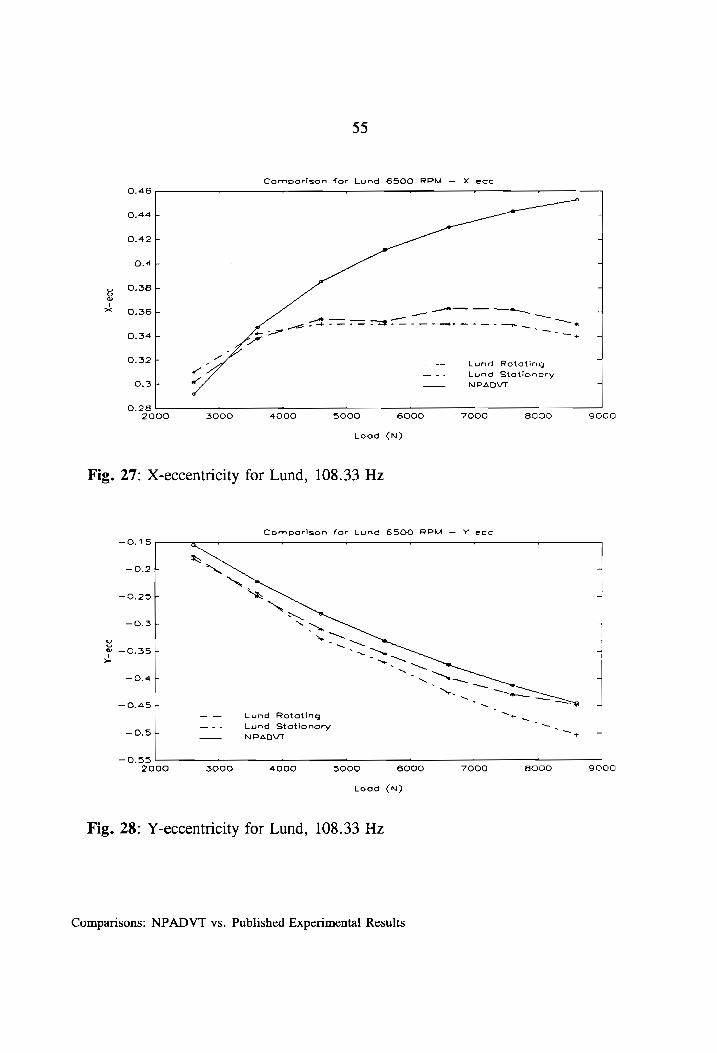
55

Comparison for Lund 6500 RPM — X ecc

0.46 r — — T r

0.44 r _

O.42+ 7

O.4- 7

o O.3SBF 7] @

1 ~< O.36- |

0.344 "

0.324 . _— Lund Rotating T ~ —-- Lund Stationory

O.3Fr —_— NPADVT 7

0.28 2000 3000 4000 S000 6000 7000 80900 9000

Lood (N)

Fig. 27: X-eccentricity for Lund, 108.33 Hz

Comporison for Lund 6500 RPM — Y ecc -0.15 . s r r

| o Ni a !

Y-ece 1 O Ul ul T

I © hb

ul T

-— Lund Rotating ~

—--: Lund Stationary ™ — NPADVT —O.55

2000 3000 4000 5000 6000 7000 BO00 9000

Lood (N}

Fig. 28: Y-eccentricity for Lund, 108.33 Hz


56

Percentage Error for Lund 2000 RPM, Stationory Probes

15 —

10 - re °

a N\, eee oe

= aa S Sb N\ 7 - 4

=< =e S ~ ae ST

e-em ~ _ & OF > ~~,

ww ™—,; > To

S ~~ Le —-5Sk ™— 4 3 ~~ & ™

re ™ — —10F- ae - 6 Y-error om 7

_- x—errar — —

—15 . —— — — 2000 3000 4000 5000 6000 7000 8000

Lood ¢(N)

Fig. 29: Percent error for Lund, 33.33 Hz (Stationary Probes)

Percentage Error for Lund 2000 RPM, Rotating Probes 106 ——— r Y — 7

™~ 5 ~~ 4

= ™~ = NN . oL —_— 4 5

S \ 4 L -- —_— -_— ™~ o

& -° / . N\ Te 7” 7

S a ~~ e104 Y — 4 S G - -* “~~

ne _7 ~,

157 -" o-p Y-errar 7

—-— X-errar

-20 . ; — — — 2000 3000 4000 3000 6000 7000 8000

Lood (N)

Fig. 30: Percent error for Lund, 33.33 Hz (Rotating Probes)


37

Percentage Error for Lund 3500 RPM, Stationory Probes

10 TF T T ~ F

am” we wrote 2 5k N\ eM ~~ eo geen 4

2 -a _ ae - o = | a“ ™.,

=z a“ ™, —S- . ~ 4

oe —™ g ~ . ew -10b ~~

: ~ 5 ~~ LY ~15- ~~ ~

a ™—

Be ™ -—20F oe -o Y-error ~~ _

—— X—-error ™ +

—25 , : . — . ‘ — 2500 3000 4000 50006 6000 7006 8000 S000 10000

Lood ¢N)

Fig. 31: Percent error for Lund, 58.33 Hz (Stationary Probes)

Percentage Error for Lund 3500 RPM, Rotating Probes 15 T tT T i T T T

—— *—error

10 r ~“ e-c Y-error 4

e ~ »

Sst N J

: \ = oF NY 4

!

2 Nee @ a” ~ = -5 L — ° SN ~ - 7 : a \ Ne ene a § “ ~ 2 —10F - ™— 4 % ° A ~~

ae a ~~ ~~, — —15b ~~ 4

™, ™—

™— —20 — : , — . . — =

2000 3000 4000 5000 6000 7000 BOOO 9006 410000

Load (N)



% err

or:

100¢

(exp

-

NPAD

VT)/

exp

Fig.

% err

or:

100+

(exp

-

NPAD

VI)/

exp

58

Percentage Error for Lund 5600 RPM, Stotionary Probes

20 —+

15 ~-- eS LL e---7-: e-~—._. “—<e—- —o- 4 ~~e lL 5

10 S

3 ~ 4

™

o ™ ~~ 7

™— ™

-5 ~, _

NY —16 _ 4

15 ~ J ~~

—_— X—error ~~,

-—-20 a-a Y-—error — — 7] ee

-25 , , — , __* 2000 30090 4000 5000 6000 7000 8000 9000

Lood ¢N)

33: Percent error for Lund, 83.33 Hz (Stationary Probes)

Percentage Error for Lund 5000 RPM, Rotating Probes 16 r , r —.

—- ~ ae

Be-T "Sey

S NY ~~ - ~e. 4

N, TS mee ~~ a

™ ™~ ~o 7 -

o we 4

NN ™,

-5 ~ 4

™

™ -10 — ~~ 4

™ ~w ~~

-—15 —-— “—error — | -—-o Y-error ~~

~~

—~20 ‘ . _. : ‘ .

2000 3000 4000 5000 G900 7O00 8000 g000

Lood (ND



% err

or:

100«

(exp

-

NPADVI)/exp

Fig.

% err

or:

100*

(exp

-

NPADVT)/exp

59

Percentoge Error for Lund 6500 RPM, Stationary Probes

15 — =— ~ mN ~- — ~ -—@--—--—- aoe LOL

10 ~~ ae Te ed ~y-

5 ™ 4 ™

™ oO ~4

A -5 NS 4

SN -—10 ™, ~ 1 -15 ™ 4

™, ~

—29 ~~ 4 Ne

—-25 — ee 7

—- ®—-error —™ -30 =m -6 Y-error ~~ 4

~~

-35 ‘ , . ‘ ‘ ' 2000 3000 4000 S000 6000 7O00 8000 9000

Lood (N)

35: Percent error for Lund, 108.33 Hz (Stationary Probes)

Percentoge Error for Lund 6500 RPM, Rototing Probes 15 r + 7

10 “~~ wee LL 4

“7: “ere eee —o. 5 ~ ee a" ~ ~ om

o ~~ ° 7

™ ~5 ™ 4

™ ™s.

—10 NN 4

45 ™ \ 4 —

—

—20 4 ~~,

-— xX~—erroar |

—-25 e-06 Y-error ~.

™ ~30 Pr , , , , *

2000 3000 4000 S000 6000 7000 8000 go00

Lood (N)




The plots of Fig. 21 through Fig. 36 again suggest problems with the cross-coupled

effect, as pointed out in the discussion of the comparisons of Ref. 30 results. The

analytical X-positions generated by NPADVT, although generally within 20% of the

experimental results, do not exhibit the same trends as the experimental results.

Interestingly, the results from both Ref. 30 and Ref. 18, which were obtained with the

same test rig, both exhibit the same trends in the x-position error. In both cases, the

NPADVT results are too small at low loads, and too large at higher loads. This

effect does not seem to be an artifact of the test rig, as the same trends will be seen in

the comparisons for Ref. 29. The Y-position generally exhibits closer agreement,

both in position and general shape. In addition, the comparison between experimental

data and an analysis with a more sophisticated thermal model than NPADVT in Ref.

18 shows similar trends. The implications of these trends have been discussed above,

and will be discussed further in the conclusions.

3.4 Comparison for Someya #2

Reference 29 is a compilation of Japanese work in the area of fluid-film bearings.

Three of the eleven experimental data sets are for plain axial-groove bearings, contain

sufficient information and are applicable to this work. The results are not identified


61

as to researcher or location. The first of the data sets to be examined is experimental

data set two. The test rig employed is of the floating bearing/rigid shaft type.

Loading is by air bellows. Both dynamic as well as static data are presented in

tabular as well as graphical form.

3.4.1 Data

The data used for comparison purposes, are from Ref. 29’s Tables 3.2.1 and 3.2.2.

These tables present the operating conditions as a function of a Sommerfeld number

(Eq. (5),) computed by assuming an effective oil temperature based on inlet and outlet

oil temperatures.

5 = BM SY (5)

Where:

p = Viscosity N = Revolutions per Second

P = Load per Unit Projected Area

R = Shaft Radius C = Radial Clearance

This somewhat artificial Sommerfeld number will be the independent variable for the

comparisons (the Sommerfeld number computed by NPADVT is generally slightly

different for the same input conditions). The oil used is identified as #90 Turbine oil,

with a viscosity of 27.37 mPaes at 40 degrees. Sufficient data was provided to fit a


62

two parameter temperature-viscosity equation as in Eq. (4). The bearing model used

is as follows:

Diameter: 100 mm

Length: 100 mm

C,/D ratio: 0.00210

Weep hole Dia: 0.2 mm

Oil inlet Dia: 6.35 mm

Grooves: O and 180 degrees from horizontal


The data from Ref. 5 and the NPADVT results for shaft eccentricity versus the

Sommerfeld number reported in Ref. 5 for speeds of 50, 100, 150, 200 and 250 Hz

are graphically compared in Fig. 37 through Fig. 46. Fig. 47 through Fig. 51 present

the same data as a percentage error (100 x (NPADVT - experimental) / NPADVT).

Note that the percentage error is expressed somewhat differently than before. This

change is required because one of the experimental points is reported as having a 90

degree attitude angle, which corresponds to a zero y-position; the previous expression

for percent error will not work for this case.


63

Comporison for Sameyo #2, about 3000 RPM, X—ecc 0.5 T T T T T T

X-ecc

——— NPADVT

7

0.25 0 0.05 o.1 0.15 0.2 0.25 O.3

Someyo Sommerfeld #

Fig. 37: X-Eccentricity Ratio for Someya Test 2, 50 Hz

Comparisan for Someyoa #2. about 3000 RPM, Y~ecc

0.35 0.45

—9.1 v Y T T T T

NPADVT

0 0.05 0.1 0.15 0.2 0.25 0.3

Someyo Sommerfeld #

Fig. 38: Y-Eccentricity Ratio for Someya Test 2, 50 Hz


0.35 0.4 0.45

64

Comparison for Someya #2, about 6000 RPM, X—ecc 0.55 r —- - - .

X-ecc

0.2557

Someya Sommerfeld #


Camporison for Someyo #2. about 6000 RPM, Y—ecc 0 , 7 s r 7

—-O.6F

Someysa Sornmerfeld #



65

Camporison for Someyo #2, GOOO RPM, xX—ecc 0.5 _ . _ .

O.35F-

X-ece

O.23-

O.2 t —-- Someya 4

—— NPADVT

o o.1 0.2 6.3 0.4 0.5 0.6 0.7

Someyag Sommerfeld #


Comporison for Someya #2, 9000 RPM, Y—-ecc

—~-O.6 Fr

-0.7 ‘ 1 a 1 4 —

o 6.1 0.2 0.3 0.4 0.5 0.6 6.7

Someya Sommerfeld #



66

Comporison for Someya #2, 12000 RPM, X—ecc 0.5 , , —— r — .

X-ece

Oo ul 7

——h.

oO 0.1 0.2 0.3 0.4 a.5 0.6 C.7 0.8

Sorneya Sommerfeld #


Comporison for Someys #2. 12000 RPM, Y-—ecc

0

~—O.1b 4

—O.2/ 2

Y foal ~

—a.4b 4

—-O.5 L. 4

—-0.6 el al 4 el 1 el, aL

Oo 0.1 0.2 0.3 0.4 0.5 0.6 0.7 0.8

Someya Sommerfeld #



67

Camporison for Someyo #2. about 15000 RPM, K-—ecc

0.5

0.454 1

0.4b 4

0.354 |

a qj)

@ a.3b x |

o.25+ J

o.2/ 4

O.15b a

0.1 _ . 4 _ . _ 0 0.1 0.2 0.3 0.4 O05 0.6 0.7 0.8

Sorneya Sommerfeld #¥


Comporison far Someyo #2, about 15000 RPM, Y—ecc oO T T T T T T =

el

o 0.1 0.2 0.3 0.4 0.5 0.6 0.7 0.8

Someya Sommerfeld #

Fig. 46: Y - Eccentricity Ratio for Someya Test 2, 250 Hz


68

Percent Error for Someys Test #2, about 3000 RPM

30 T T 7 v ¥ r T v _

7 —

—

S Zor _ a

a _— <=

S — we “—

a 1OF 5 a a a —

i » a

S . — 5 Or re a“ <x ~ a“ Qa —T = a o-.

< TN, = —1OF ra ee

S Tee 5 ym x —20F — Y-error ie

—_—s- X—error ~“~~s

— 30 ° 0,905 O.1 0.15 0.2 0.25 0.3 0,35 0.4

Someya Sommerfeld #

Fig. 47: Percent Error for Someya Test 2, 50 Hz

Percent Error for Someyo Test #2. about GO00 RPM

30 r T T T T

204+ a /™

™ S L & / ~

1 a ~o —_— — J —-- ~ at o oF e \ wv 1

| \ —~10Ob .

3 \ 4 .

Ss —20 ee

3 OTe = —30F ~

: a aD —40F ym

Be —_— Y-error ee —-5O0- —-- X—-errar oN

~

—60 1 _ 1 4 i _.

oO 0.1 0.2 o.3 Q.4 0.5 0.6

Someya Sommerfeld #



69

Percent Error for Someyo Test #2, 9000 RPM

100 ~~ T 7 T vr T

BOF _ —

S a“ — oD BOF —"

4 ee

S —_— a = 40 z a

S a_ v ZOr a —— —

t a — ——

“ _— 3 OF a

2 os > —-20F- ~

S ~ ~ = nao S os vo -60F er

Be ; —_— Y-error Te —80 —-- X—errar Te

~~ 5

— 100 7 : — 4 oS 0.1 0.2 0.3 0.4 0.5 0.6

Someyoa Sommerfeld #


Percent Error for Someyo Test #2. 12000 RPM 100 t v a t ~ ¥ rn

_—- — Y—-error —

—-- X—error a

BO a = © L ed —

S — ~~, 60Fr “—

a — a 2 aT

\ 40 & y x ~

= & a“

& 207 ‘\ < > O, a

3 ss

BP NY a — 2 ™

20h ee LL Lee °

-40 1 — ‘ — 1 — .

o Q.1 0.2 0.3 0.4 0.5 0.6 0.7

Someya Sommerfeld #



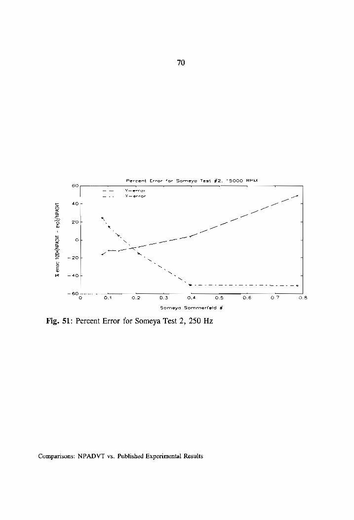
70

Percent Error for Someyo Test #2. 15000 RPM 60 Tv T ¥ t t ~~ -F tT

—_— Yoerror

—-- X—error _—

5 407 a o —

S a = 20b ‘ — e — wu QR a

' \ - “a

S . — 2 o i “\ —_— —

a . oe — = — oo 5 a - —-20F ~

S oN v N

ae —40F- . ~

Wee eee eae ee ee le

-60 ‘ _ 1 _. ‘ 4 1

Co a. 0.2 0.3 0.4 0.5 0.6 a.?7

Someyo Sommerfeitd #



71


The NPADVT analysis for this bearing does not agree with the experimental results

as well as the previous comparisons. Part of this is likely to be due to modeling

error, as no data were presented in Ref. 29 for the feed groove extent, weep hole

diameter and inlet hole diameter. This source of error would be in accord with the

fact that the error is most apparent at larger Sommerfeld numbers (corresponding to

relatively lighter loading), where the effects of feed groove extent would be most

noticeable. Other than an attempt to get the NPADVT temperature rise through the

bearing to be reasonably close to the experimental temperature rise by varying the

weep hole size, no attempt was made to match results by varying groove extent or oil

inlet hole diameter. Zero offsets do not seem to provide an explanation of the

differences either, as the NPADVT results are both larger and smaller than the

experimental data. In general, the results exhibit similar trends as before. The

NPADVT predicted Y-position is generally close and has the nght general shape

(especially at the lower Sommerfeld numbers); the X-position generally exhibits the

wrong shape, even if the absolute position is close.


72


The second data set from Ref. 29 used as a basis for comparison to the NPADVT

analysis is experimental data set number three. These data were obtained with a

floating bearing/rigid shaft test rig with pneumatic loading. Again, both tabular and

graphical results are presented for static and dynamic characteristics.

3.5.1 Data

The data set used is that of Tables 3.3.1 and 3.3.2, which present the static operating

characteristics as a function of Sommerfeld number. Since the oil temperature, etc. is

consistent from speed to speed, the results will be presented for 26.7, 66.7, and 100

Hz as a function of load. The oil used for this set of experiments is identified as an

ISO 32 oil, with a viscosity of 18.4 mPaes at 50 degrees. Sufficient data are

presented for a two parameter viscosity-temperature relationship of the form of Eq.

(4). The geometric data for this bearing are also more complete than for the previous

data set. The bearing model used is as follows:

Diameter: 100 mm

Length: 50 mm

C,/D ratio: 0.0028


73

Weep Hole Dia: 2mm

Oil Inlet Dia: 15 mm



(actual groove is 1 mm deep)

The data from Ref. 29 and the NPADVT results for shaft position for 26.7, 66.7, and

100 Hz as a function of load are presented in Fig. 52 through Fig. 57. Fig. 58

through Fig. 60 present the comparison as a percent error (100 * (exp - NPADVT) /

exp).


74

Comporison for Sameyo #3, 1602 RPM — * ecec 0.46 + —r r 7

X-ecc

O.395F

—--: Someya we |

O.3B Fr ——_. NPADVT ~ 0.37 2000 2500 3600 3500 4000 4500

Lood (N)

Fig. 52: X-Eccentricity Ratio for Someya Test 3, 26.7 Hz

Comporison for Someyo #3, 1602 RPM — Y ecc —0.6 7 — r

—0.62 tT

~O.645-

I Q a Qa T

~O.72/+

—~O.74b

—O.76+ —-0.78 2000 2500 3000 3500 4000 4500

Load (N)

Fig. 53: Y-Eccentricity Ratio for Someya Test 3, 26.7 Hz


75

Comporison for Someyoa #3, 4002 RPM — X ecc

X-ece

0.38 -

O.36F

—

— NPADVT

—-- Someya

—* * - ” 0.34

1000 1500 2000 2500 3000 4500 4006

Load (NJ)

Fig. 54: X-Eccentricity Ratio for Someya Test 3, 66.7 Hz

Comparison for Someyo #3, 4002 RPM — Y ecc

4500

—0.65 L

> v —-

—-- Someya mM

— NPADVT -O0.7

1000 13500 2000 2500 3000 3S00 4000

Lood (NJ

Fig. 55: Y-Eccentricity Ratio for Someya Test 3, 66.7 Hz


4500

76

Comporisan for Sameyo #3, 6000 RPM — X ecc

X-ecc

O.25 5+

0.1S + _—-- Someyo J

y —_— NPADVT "200 400 500 800 19000 1200 1400 1600

Load (N)


Comparison for Someyo #3, 6000 RPM — Y ecc 0.05 1 7 r r r

—O.OS-

—0.25 |

—0O.3 200 400 Boo 800 1000 1200 1400 1600

Load (NJ)



77

Percent Error for Someyo #3, 1602 RPM

-2 _—-4

-3 Leet ~~ J

~— ee oT oe -4r —_—— — arm _—* 7

LY ee S -5po em ~ 1 6S € 6 ™ : =z r ™~,

| ~~

~_7 4

& t _ S -al SN S ~9P m™ 4 b ~~,

re ~10F ~ _

—_— x—error NN —1T1t —-- Y-error “NOT

—12 , A — ‘

2000 2500 3000 3500 4000 4500

Lood ¢N)

Fig. 58: Percent Error for Someya Test 3, 26.7 Hz

Percent Error for Someyo #3, 4002 RPM 196 v — — r r —-

oe woe. ~ eee or ee —_ - 5 wo

= 5 , 7

= o =< -sh 4 =

' _-— X— error 2. —10F —-- Yo error 4

& S + S ~15+ NN 4

: ~ & -~20F ™ 7

pe ~~ a

— ~~

-25+ me TF 4

—3BO ‘. 1 1 1. 1 1

1000 1500 2000 2500 3000 3500 4000 4500

Lead (N)>

Fig. 59: Percent Error for Someya Test 3, 66.7 Hz


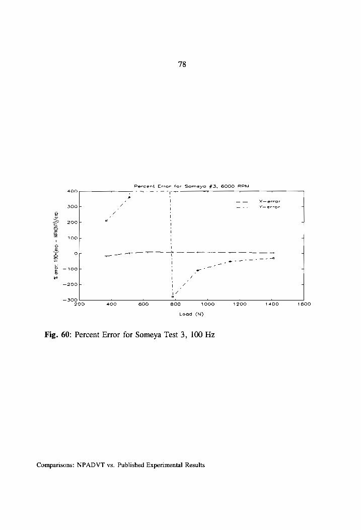
78

Percent Error for Sameyoa #3, 6000 RPM

409, —-m-- ee i —— —

s . | —_ X— error

300F , a \ —-- Y—error 7

g / 2 ’ I

S 2004 o ; 4

a \ = ‘

; 100 {

a ' ze (

> OF ae oe tee eee Sa 4

S — _-2 _ ' rn

2 —-100F ' = -a 7

re 4 —200 1 4 4

,

a —300 1 1 ‘ 4 ‘ 1‘

200 400 600 BOO 19000 1200 1400 1600

Load (N)



79


The results for this set of comparisons are interesting. At lower Sommerfeld

numbers, the NPADVT results look quite good. It would also appear that some of

the differences between experimental and NPADVT results could be caused by zero

offsets. The Sommerfeld numbers in this data set are somewhat larger (0.2 to 2.21)

than in the previous data set. In general, with the exception of the 26.7 Hz Y-

position and the 66.7 Hz X-position, the NPADVT analyses yield very good

predictions (the percent error plots may be a bit misleading at the lower

eccentricities). It is not apparent why the 26.7 Hz Y-position and the 66.7 Hz X-

position do not follow in line with the rest of the comparisons. Modeling error does

not quite seem to be the answer, nor are these two Sommerfeld numbers close to each

other.


The final experimental data set from Ref. 29 is that for test bearing number five.

These data were obtained with a floating bearing/rigid shaft type test mg, with manual

mechanical static loading. Results for static and dynamic characteristics are presented

in both tabular and graphical form.


80

3.6.1 Data

The oil used is identified as a #90 Turbine oil, with a viscosity of 13.41 mPa®s at 50

degrees. Sufficient data were once again presented for a two parameter equation of

the form of Eq. (4) for the viscosity-temperature relationship for the oil. The bearing

geometry data presented did not include feed groove details, so nominal dimensions

were assumed. The bearing model is as follows:

Diameter: 50 mm

Length: 50 mm

C,/D ratio: 0.00132



Grooves: O and 180 degrees from horizontal


The comparisons between the experimental data of Ref. 29, tables 3.5.1 and 3.5.2

and the appropriate NPADVT analysis are presented below in Fig. 61 and Fig. 62.

AS with test bearing number two above, the independent variable is the nominal

Sommerfeld number reported in Ref. 29. Fig. 63 presents the comparison as a

percentage error (100*(experimental - NPADVT) /experimental)).


Comparison for Someya

81

Test #5. xK-ecc

X-ecc

o bh T

O.38F

O.36-

O.34 5 0.32 ———. 1 1.

Q.1 0.2 0.4 0.5 0.6

Someya Sommerfeld #

Fig. 61: X-Eccentricity Ratio for Someya Test 5

Comporison for Someya Test #5, Y-ecc

T

I 1,

0.3 0.4 0.5 0.6

Someya Sommerfeld #

Fig. 62: Y-Eccentricity Ratio for Someya Test 5


82

Percent Error for Someyo Test #5

20 r T + T + v v

ON oe ed

= S

SS -20h% &. _”, > 4 = ~< “ee TON

~™

a e--—--—- a - —404+ 7

S *s qw ‘\ os

Ss ~-6OF : 4‘ 4 & \ . = an 7

S —B8OF : / 4 a \ ,

x Y a“

—100b —-- Y-error in 4 a

—_— X—- error ‘ Sf

-—-120 1. 1 bee a —— 1 4

0.1 0.2 0.3 0.4 0.5 0.6 0.7 0.8 0.9

Someyo Sommerfeld ¥#

Fig. 63: Percent Error for Someya Test 5


83


The comparison for this set of experimental data does not show the same trends as the

previous comparisons. The X-position is not only close in absolute terms, but it also

generally has the correct shape. The Y-position seems to be about the right shape,

but the percent error for Sommerfeld numbers greater than 0.5 is high; this difference

could be caused by a zero offset. These seemingly anomalous results could also be

the result of a number of other factors; among them, this bearing is only half the

diameter of the other bearings examined. The smaller diameter could result in

different mechanisms dominating the difference between experimental results and

NPADVT analysis than in the larger bearings. The effects of cavitation or feed

grooves, for example, might be more significant in the smaller bearing.

3.7 Comparison for Andrisano

The final experimental data set to be examined is from Ref. 3, A.O. Andrisano’s

1988 Journal of Tribology article. Although this article primarily focuses on a fairly

sophisticated investigation of the surface temperature of a rotating shaft, results are

presented for shaft locus as a function of load and speed. This work made use of a

floating bearing/rigid shaft test rig at the University of Bologna (Italy). This rig is


84

loaded with dead weight through a link mechanism. This set of results is especially

interesting because the feed geometry is a single groove, located at the top of the

bearing (the other data sets used two horizontal grooves). Although it was hoped that

this data would shed light on the possibility of problems with feed groove effects not

modeled in NPADVT, the experimental data exhibit some unusual trends that prevent

strong conclusions from being reached.

3.7.1 Data

The data used for comparison purposes, are those of Andrisano’s Fig. 9. This figure

presents relative eccentricity as a function of load and speed for an ISO 46 oil with a

viscosity of 25.96 mPaes at 50 degrees. Two temperature-viscosity points are

presented, which allows a relation of the form of Eq. (4) to be specified. A nominal

lubricant specific heat and density are also presented. The bearing model used is as

follows:

Diameter: 45 mm

Length: 45 mm

C,/D ratio: 0.00133




85

Groove: 90 degrees from horizontal


The data scaled from Andrisano’s Fig. 9, and the NPADVT results for shaft

eccentricity ratio for 10, 20, 30 and 40 Hz are graphically compared in Fig. 64

through Fig. 71. Fig. 72 through Fig. 75 present the same data as a percentage error

(100 x (experimental - NPADVT) / experimental).


86

Comporison for Andrisano, 600 RPM, X—ecc

X-Eee

© b wi '

oo

_

NPADVT

Andrisaono

600 800 1000 1200 1400 1600

Lood (N)

Fig. 64: X-Eccentricity Ratio for Andrisano, 10 Hz

Comporison for Andrisona, 600 RPM, Y—ecc

1800 2000

0 ¥ v T t v

a—o NPAOVT

—_——n Andrisono

8B 1 1 2 ‘4 a

600 Bao 1000 1200 1400 1600

Lood (N)

Fig. 65: Y-Eccentricity Ratio for Andrisano,10 Hz


87

Comporison for Andrisona, 1200 RPM, X—ecc

0.55 1 +

O.5-

O.4SF-

O.4- y a

Lal

> 0,356

O.3-+

O.25¢ o—o NPAODVT

—— Andrisono

0.2 . : : ; 500 1000 1500 2000 2500 3000

Lood (N)


Cormporison for Andrisano, 1200 RPM, Y—ecc T

0 wv ms ~T

—O.71b

—-O.2F

g i —-O.3F >

~O.4b

_osl o»—o NPADVT NN

— Andrisono |

—9.6 , : : , 500 1000 1500 2000 2500 3000

Lood (N)

Fig. 67: Y-Eccentricity Ratio for Andrisano, 20 Hz


88

Cormmporison for Andrisono, 1800 RPM, X—ecc

— —_

0.25 _ _—_ oo o—o NPADVT

—_——n Andrisono 0.2 ; ;

500 1000 1500 2000 2500 3000

Lood (N)


Comporison for Andrisano, 1800 RPM, Y-—ecc

o—o NPAOQVT

—_——* Andrisano

—0.6 1 1 . :

500 1000 1500 2000 2500 3000

Lood (N)



89

Comporitson for Andrisaono, 2400 RPM, K—ecc

0.55 —

X-Ece

© tn on |

O.2+ _— a——o NPADVT

— —n Andrisano

500 1000 1500 2000 2500 3000

Lood (N)


Comporison for Andrisono, 2400 RPM, Y—ecc

| o an T

Y¥-Eec

| 0 rN) wn |

== NPADVT b

—0.45 J ae

—_——« Andrisono -0.5 , ,

500 1000 1500 2000 2500 3000

Lood (N)



90

Percent Error for Andrisono, 600 RPM

70 — . ¥ qT 7 ¥ T T

6OL Te 4 an

a — — ~ 5SOr — = wu ~~

—~ ~~

5 — 40h — 4 a ~~ o ~~ =z —

\ 30 — \ 4

¢ ~ 2 SS ‘. 104 4 5 ™~ = NN

By OF ~~ 7

NN sob ee Xcerror . mR Yo-error

-—20 . : 4 : ; : 600 Bao 1005 1200 1400 1600 18900 2000

Load (N)

Fig. 72: Percent Error for Andrisano, 10 Hz 3

Percent Error for Andrisano, 1200 RPM

60 7 T 7 T

40+ _-- 4

a a ° x ed & a

bee ws — € 20 ee

= a a” -

= OF _ - 4 i :

& ~ , & A eee S —20 [— “er ee _~

o \ / ~~ —_ oo — —_— —e - — ~ \ f — ° -—-40F ’ “2

a \ /

BS \ a -—-60- . ,

NZ oe —o X—~error |

a - Yoerror

—- 80 : . ; 7 500 1000 1500 2000 2500 3000

Load (N)

Fig. 73: Percent Error for Andrisano, 20 Hz


91

Percent Error for Andrisano, 1800 RPM

40 Tv T T T

20 et —- Ft

~~

w

= OL : 4

= 7

3 —20+ “ 4

S ” < { —40F- ™~ as ‘ a

aes —, —

a _ 6O a Ne _ a , ~ ~~ an a

oS ~~ Lh e~ - a“ ~~

2 “

a —- 80 ° 7

S ; Un qu - Be OT 100F- _ “ 5

—120F _7 eo — X—error = a

ane a Y-error

—1 40 =~ 1 a 4 1

500 1000 1500 2000 25900 3000

Load (NJ


Percent Error for Andrisana, 2400 RPM

S50 ¥ Fe T v

OF aosccoesoT 4 a - = _- =>

a a

ZB -sob —_— ee 2 w -_— a”

' — ~e ~ a — / °

@ —100+ - _ & a“

Ss 7

2 —150F- 7 7

S _-" i Deo

ae ant —2007F ee -

- —o X—error

am Y-error

—250 ; : . * 500 10606 1506 2000 2500 3000

Lood (N)



92


As mentioned in the introductory remarks to this data set, the data exhibit some

unusual trends. In particular, the X-eccentricity ratio does not change smoothly as

load increases; rather, for some reason, it exhibits a discontinuity at 2500 N load for

20, 30, and 40 Hz (the 10 Hz data does not include loads above 2000 N). This

discontinuity is not simply the point at which the X-eccentricity ratio begins to reduce

with increasing load, as would be expected for a plain journal bearing. In the 20 Hz

(Fig. 66) case, the X-eccentricity ratio does begin to decrease, but for the 30 Hz and

40 Hz (Fig. 68 and Fig. 70) cases, the X-eccentricity ratio decreases at 2500 N, then

increases again at 3000 N. This behavior is unusual. One possibility is that discrete

test runs were employed for each load/speed point (or so the article implies), which

could easily result in zero shifts, or slightly different thermal conditions.

Uncertainties in the shaft position measurements do not really provide the answer.

Although they are not specified, they would have to be on the order of 20 percent to

explain the unusual behavior.

Despite this possible problem, it was hoped that the difference between the two oil

grooves at 0 and 180 degrees employed in the other works reviewed, and the single

groove at 90 degrees employed in this work, might shed some light on the influence


93

of feed groove effects. Unfortunately, none of the NPADVT results are sufficiently

close to the Andrisano experimental results to draw strong conclusions. The

differences are not altogether surprising, as the NPADVT model is not very refined -

it spreads 50 nodes out over 345 degrees of arc width, as opposed to 50 nodes over

180 degrees of arc for the other bearings examined (50 circumferential nodes is the

maximum allowed in the current version of NPADVT). Indeed, this model would

begin to diverge if many more than 5 temperature-viscosity iterations were employed

(one possible solution to the limitation on number of nodes would be to use a smaller

arc for the active pad, as much of the top of the bearing is most likely cavitated - this

has not been explored). Even so, some general observations are possible. There is

some support for the possibility of feed groove effects, as the X-eccentricity ratio

results are in general closer than the Y-eccentricity results. The X-eccentricity ratio

results do not, however, exhibit the correct shape relative to the experimental results.

Later results presented for the VPI rig will show that the pressure effect does not

seem to be the cause of the discrepancy between analysis and experiment. The

comparison with the data of Ref. 3 does, however, point out the need for a higher

limit on the number of circumferential nodes for bearings with pads encompassing

such a large angular extent.


Chapter 4

VPI & SU Test Rig

4.1 Introduction and Orientation

This Chapter is devoted to describing the VPI rig in preparation for the presentation

of results from the rig in Chapter 5 and 6. Both a summary description and a more

detailed description are included in this chapter. This chapter also discusses

instrumentation calibration issues and includes an uncertainty analysis for

displacement and load.

94

95

4.2 Rig History

The VPI & SU rotor dynamics research laboratory fluid-film bearing test rig (VPI

Rig), shown in Fig. 76 and Fig. 77, was designed and constructed in the mid-1980’s

by a major turbomachinery manufacturer to support the development of new

compressor bearings. The rig was only run briefly before this program was

discontinued. The rig was eventually donated to the university in the spring of 1989.

This test rig is of the fixed test bearing/floating shaft type. During the spring of

1990, as an undergraduate research project, the author restored it to a temporary

working configuration and determined that it was still functional. The rig has since

been permanently mounted on a large (7700 Kg+) reinforced concrete pedestal. In

addition, adequate instrumention and automatic controls for operation and test control

have been added.

Chapter 4 - VPI & SU Text Rig

96

ee ee ; _ Ee

‘oan RRA. ae rate Pee ee He _ _ Se pages nese eeseantes wae He ie ee ee ae ge ee peta!

ee eine art

: ae Le penn eee ee ee ecetaaen eee,

eee oN eas ere teere es ee a pies

a eee. saints ee Be ee ee is _ ie sande Bieter sae ce ae ee ae

wach pe. . a8 oe : ect ee

Cea sree ree

ete eae COS

Fig. 76: VPI & SU Fluid Film Bearing Test Rig


97

NLL ee re:

!

G

'tog 1 1008 | a gH

bay

4 {

Note: All Din. in nn

Legend

A - Test Bear ing Housing

B - Shoft Displocenent Probes (Inboard ond (hitboard of Bear ing}

C - Loading Magnets Housing

D - Key Phosor Pickup

E - Reor Shaft Displacenent Probes

F - Air Turbine

G - High Speed Coupling and Torque Sensor

H - Reinforced Concrete Foundatl on

Fig. 77: Test Rig Sketch


98

4.2.1 Summary of Test Rig Capabilities

Speed range: 3 Hz - 530 Hz,

Driver: 30 kW air turbine,

Loading: Approx. 6.9 KN shaft load; 5.7 KN bearing load; two axis loading

(up-down, left-right),

Test Bearing Capacity: 203 mm Dia. by 90 mm deep cavity, shaft designed to

accept sleeves to adapt to bearing diameter,

Oil System: 0.04 m? heated oil reservoir, 500 cm*/s vane oil pump with a

pressure rating of 0.61 MPa,

Instrumentation: Shaft position (3 planes), oil temperature and pressure,

bearing temperatures, shaft speed, shaft load, and turbine output

torque,

Data Acquisition: Combination of stand alone and microcomputer hardware,

Control and Supervisory: Air turbine speed controlled by a custom PC based

controller and two pneumatically operated valves, separate

overspeed/overtorque shut-off controller, air turbine shut-down for low

oil level in test bearing and support bearing sump, or test bearing low

oil pressure. Test bearing oil temperature control with commercial PID

controller operating a pneumatic valve controlling water flow through


99

an oil to water heat exchanger, oil sump temperature with proportional

heater controller.

4.3 Detailed Description of Test Rig

The detailed description of the test rig will be broken into 5 sections:

1) mechanical details

2) magnetic loading system

3) air turbine drive

4) test bearing oil system

5) other instrumentation.

4.3.1 Mechanical Details

The VPI rig, shown in Fig. 76, and schematically in Fig. 77 is designed using the

rigid bearing mount/floating shaft paradigm. The test rig, constructed for the most

part of type 410 stainless steel, has an estimated mass in the vicinity of 450 Kg, and

is in turn securely bolted to a 7700+ Kg reinforced concrete foundation. This

combination provides a very rigid bearing support. For static testing, the rig is

essentially fixed in place. Mechanically, the rig is also extremely stiff, constructed

from 25 mm and 38 mm plate, securely bolted together. The bearing housing is a


100

single piece of stainless steel, 330 mm wide by 375 mm tall by 127 mm deep. The

shaft is also fabricated from type 410 Stainless Steel, treated to Re 36/39 (yield

strength of 1200 MPa vs. 500 MPa for untreated). It is 101.6 mm in diameter over

most of the 0.762 m span between bearing centerlines. It necks down to 29 mm at

the rear support bearing and to 31.8 mm at the test bearing (this end accepts the

sleeve to adapt to bearing diameter). At the loading magnets, the shaft is cut down to

63.5 mm diameter to accommodate the laminates required to reduce eddy-current

losses in the magnetic loading system. These laminates, of 0.36 mm thick Hiperco 50

(a high performance magnetic alloy), bring the shaft outside diameter to 108 mm

diameter for the length of the magnetic loading system (described in the next section).

The measured shaft slope due to load, across the test bearing sleeve (assumed to be

rigid), is 6x10* mm/mm. The maximum shaft deflection relative to the bearing

centerline is 0.095 mm at the loading magnets. Appendix A contains a detailed sketch

of the measured shaft deflection.

The rear support bearing is a 30 mm ID by 50 mm OD, duplex angular contact ball

bearing, mounted in a spherical housing to facilitate alignment. This bearing is

lubricated and cooled by an oil mist lubrication system and is rated for continuous

operation at the rig’s maximum speed and load. This bearing has an experimentally


101

determined stiffness of 35 MN/m. The bearing is sealed on either side with a

windback seal.

The test bearing is mounted in a carrier housing which matches the test bearing OD to

the test rig bearing cavity ID of 203 mm. The fits on this housing are between line-

to-line and 0.025 mm loose. The cavity of the bearing housing is approximately 70

mm deep, with openings for oil drains on the bottom, an offset oil inlet on the top,

and a removable front cover. The shaft seal is again a windback design. The shaft is

aligned to be parallel to the housing bore to 5.7 mm/mm. This alignment was

performed with the test bearing in place with the following procedure:

1) load shaft down lightly and note dial indicator reading at 3 O’Clock

position.

2) rotate shaft and note dial indicator reading at 9 O’Clock position.

3) adjust rear support bearing horizontal position until these two readings match.

4) balance shaft weight with up magnet and load shaft to the left.

5) adjust rear support bearing until 12 O’Clock and 6 O’Clock readings

match

6) check horizontal position

This procedure was performed with the test rig at "cold" conditions. After the rig

warms to operating temperature (43.3 degree oil temperature), the bearing housing

grows by approximately 0.08 mm. To allow for this increase, the rear support bearing


102

was adjusted upwards by approximately 0.05 mm. With this adjustment, the warm

bearing clearance, as indicated by a lift check, agreed with the original cold clearance

plus an allowance for thermal growth.

The 30 kW, 3 Hz to 530 Hz air turbine drive is mounted to the rear bearing housing

support through a four arm strain bridge (see Fig. 77). The turbine output shaft and

the test rig shaft are coupled through a floating, double diaphragm coupling which

offers very little resistance to shaft angular motion. The air turbine employs grease

lubricated bearings and is rated for continuous operation at maximum speed. The

compressed air for the air turbine drive is supplied from a large diesel compressor

located outside the building through approximately 45 m of 50 mm diameter PVC

pipe. Air filters, a shut-off valve and two pneumatically operated throttling valves

(for speed control) are located several meters above the air turbine drive on a wooden

support structure. This arrangement allows a reasonably long length of vertical PVC

pipe to be attached to the air turbine in an attempt to minimize the influence of the air

supply piping on the torque reading from the torque bridge. Unfortunately, the

wooden structure is not rigid enough, and moves enough to measurably change the

torque bridge zero. The torque bridge zero is also strongly affected by temperature

changes. The rig electrical power and water supplies are also attached to this

Structure.


103

4.3.2 Magnetic Loading System

A magnetic loading system is employed to load the shaft, which in turn loads the test

bearing (see Fig. 78). This non-contact loading approach eliminates some of the

mechanical difficulties of loading a bearing via a rotating shaft. As designed, the

loading system consists of four axial electromagnets arranged at right angles, thereby

allowing loads to be applied in any arbitrary radial direction. Currently, only three

magnets are installed (up, down, and left). These magnets are capable of applying a

static load of up to 6900 N to the shaft at a nominal 0.5 mm air gap. Depending on

the location of the test bearing centerline, between 80 and 85 percent of this load is

applied to the test bearing. Each magnet is mounted on a 8900 N capacity load cell

to provide a measurement of applied load. The specifications on these load cells

suggest a maximum combined bias and random uncertainty of plus or minus

approximately 32 N. This uncertainty, and means of reducing it, will be discussed in

greater detail in a later section.

The loading magnets are constructed around a U-shaped piece of solid Hiperco 50,

with 700 turns of wire around each leg. The eddy-current losses, due to the solid

core and the inductance due to the large number of turns, limits the applied load to

static or almost static (less than a few Hertz). This limitation applies only to the


104

loading magnets; the rotating portion of the shaft is laminated, and thus would be able

to operate at reasonably high frequencies. At the maximum load of 6900 N, the

magnets require 7.2 A at 58 volts.

As currently configured, the loading system does not include a true feedback control

system. Loads are set manually or under computer control by increasing the current

supplied to the magnets until the desired load, as sensed through a data acquisition

card in the PC, is obtained. This approach is adequate for the static tests associated

with this work.


105

f Loading Magnets (2 shown)

2

T5505 RIKKI

ING Noteceretatete: O

S

SOO

RIND

OO ose

o. SD

652550555

$2505

Fig. 78: Shaft/Magnet Arrangement


106

4.3.3 Air Turbine Drive

The air turbine drive system is a single stage, 30 kW air turbine, rated for continuous

operation at up to 583 Hz, Minimum operational speed is in the vicinity of 3 Hz.

The air turbine is mounted on a four arm torque bridge to provide a means of

monitoring the turbine output torque. This measured torque, however, is greater than

that caused by losses in the test bearing alone. Additional losses in the support

bearing, seals, magnetic loading system, and shaft windage increase the drive torque

above the bearing torque. A custom PC based control system, with feedback from

the turbine speed pickup (a 30 tooth gear), is employed to control speed by

modulating two pneumatically operated control valves (32 mm and 20 mm) in the air

supply line. This system controls the operating speed to within plus or minus 0.4 Hz.

The turbine speed pickup is also connected to a separate overspeed shut-down

controller. This controller will shut off the air supply with a solenoid valve if the

speed reaches an operator set limit value. This controller also contains the signal

conditioning and readout for the torque bridge. Automatic shut-down with this shut-

off valve also occurs for low oil level in either the test bearing oil sump or the

support bearing oil mist system, as well as for low oil pressure at the test bearing oil

inlet. The operator may also manually close this shut-off valve.


107

4.3.4 Test Bearing Oil System

The oil system for the test bearing consists of a 0.04 m* heated sump, a 500 cm?/sec

vane oil pump with a pressure rating of 0.6 MPa, an oil to water shell and tube heat

exchanger and a commercial PID control system which regulates cooling water flow

to control oil temperature based on feedback from a thermocouple located in the

bearing oil inlet passage. The oil is filtered through a single 10 micron filter. The

supply temperature is generally held to within +1 degree C of the setpoint

temperature. Pressure at the bearing housing inlet is controlled with a spring loaded

bypass valve, which maintains the supply pressure very close to the initial pressure

setpoint. Flow measurement is provided by a variable cross-section flow meter

(rotameter). Pressure is measured with an analog pressure gauge at the inlet to the

bearing housing. The oil reservoir temperature is maintained above the bearing

supply temperature with proportional (electrical) control of the tank heater. This

elevated temperature allows the bearing oil inlet temperature to be controlled by

modulating the water flow through the heat exchanger. Oil supply and exit

temperatures at the test bearing are measured with type J thermocouples connected to

the PC data acquisition system.


108

4.3.5 Other Instrumentation

The shaft displacement is measured at three axial locations to allow shaft angular and

radial displacements to be characterized. Two (1x, ly) eddy-current displacement

probes are installed just inboard of the rear shaft support bearing. Four (2x, 2y)

eddy-current displacement probes are installed in opposing pairs just inboard of the

test bearing. Two (1x, ly) eddy-current displacement probes are installed just

outboard of the test bearing location. The dual, opposed probe approach used at the

inside measuring location allows uniform diametral growth, such as could be caused

by thermal expansion, or centrifugal growth, to be cancelled from displacement

measurements. The magnitude of such growth can also be estimated using this

approach. The use of opposed probes also has the advantage of reducing noise,

thereby increasing resolution. Although it would be desirable, dual opposed probes

are not installed at the outboard probe location. The combination of probes used

should allow the shaft displacement at the bearing centerline to be estimated with a

sufficiently low uncertainty for present purposes (see section on uncertainty analysis

for details). These probes are connected to a stand-alone instrument which takes shaft

synchronous readings, thus allowing electronic run-out compensation to be employed.

This instrument is designed to download data to a PC and has been specially modified

to allow direct PC control of data acquisition. Each sample is composed of 32 8-bit


109

readings per revolution for 8 revolutions, for a total of 256 readings per channel per

sample. These readings are used along with a 12-bit integrated shaft centerline

reading (6.29 second integration time constant), to provide a compensated average

shaft centerline position.

Shaft speed is sensed with both a 30 pulse per revolution speed pickup in the air

turbine as well as by a one time per revolution key-phasor pulse from the test rig

shaft. The key-phasor pulse is used by the stand-alone displacement instrumentation

to provide the synchronous data acquisition required to perform electrical run-out

compensation.

Other test rig bearing temperatures are monitored with thermistor sensors installed on

the air turbine ball bearing housings (sealed grease lubrication), as well as the test rig

rear support ball bearing housing (oil mist lubrication) to enable action to be taken in

the event of high bearing temperatures.

Finally, a thermistor sensor is installed in the air turbine exhaust to help diagnose any

frosting problems in the turbine.


110

4.4 Sensor Calibration

Due to the extreme dependence of the results on the accuracy of the eddy-current

displacement probes, a great deal of effort was expended in calibrating the

probe/proximeter(demodulator)/amplifier/data acquisition instrument system. The

probe/proximeter system specifications are given by the manufacturer as: non-linearity

less than 0.02 mm, noise floor of less than 0.0025 mm (the actual noise floor seen in

testing is close to an order of magnitude smaller), with a scale factor temperature

effect of -3% at 65 degrees at a 1.27 mm gap setting (this figure agrees well with an

experimental verification of the temperature sensitivity). The nominal

probe/proximeter scale factor is 8.0 volts per millimeter. This scale factor does not

give sufficient resolution with the 0.0244 volt minimum static resolution of the data

acquisition equipment employed. Therefore, the output of each probe/proximeter is

also passed through a times five amplifier (LM318 op amp). To verify the

manufacturer’s probe/proximeter specifications and check the calibration of the times

five amplifiers, each of the probes was calibrated to the appropriate target (shaft or

bearing sleeve). For calibration, each probe was mounted on a movable fixture and

the probe measurements compared to a measurements taken with a precision dial

indicator with 0.0025 mm gradations. The amplified proximeter output was

connected to a 12-bit analog to digital board through a bucking power supply (the


111

proximeter output is negative 5 to 17 volts), and a low pass filter. These components

were calibrated as a system with a calibrated 5 1/2 digit voltmeter, specified to be

accurate to +0.0009 volts worst case. The probe calibration procedure used is as

follows:

1) Allow system to warm up,

2) Set probe offset to approximately 0.7 mm,

3) Take 9 readings at 0.025 mm increments, moving away from target,

and obtain a least squares calibration slope,

4) Take 9 readings at 0.025 mm increments moving towards shaft from

end of previous series, and obtain least squares slope,

5) Finally, take 18 readings at 0.013 mm increments moving away from

shaft, starting at initial start point, and obtain least squares calibration

slope.

Each data point is the average of 1000 points on two channels, for a total of 2000

points, over a 2 second period. The standard deviation of the data set for each data

point was very low, indicating that noise contamination of each reading was minimal.

The slope in all cases was repeatable to better than 1 percent. The maximum

deviation from linearity was 9.65 x 10* mm (this deviation may well be related to the

dial indicator used, as it occurs at roughly the same place with each probe); the

deviation from linearity is generally an order of magnitude better than this figure.


112

The accuracy specification for the 12-bit data acquisition system used for the bearing

testing is given as +0.5% of reading + 0.0192 V (this translates to +0.00125 mm).

With these accuracy figures, the +0.0025 mm uncertainty in displacement

measurements used in the uncertainty analysis should be a conservative figure.

The manufacturer of the load cells used to measure magnet load quotes the following

inspection limits for the load cells:

Rated Capacity: 8896 N

Non-Linearity: +0.20 % F.S. (17.8 N)

Hysteresis: +0.15 % F.S. (13.3 N)

Repeatability: +0.05 % F.S. (4.4 N)

Since these numbers are the inspection limits which 100% of the units must satisfy,

they correspond to a spread of approximately 3 standard deviations. Since the

uncertainty analysis for this work is based on a 95% confidence interval, the above

specifications need to be adjusted by a factor of 1.96/3.00 (the ratio of standard

deviations for 95% to 99%). The resulting specifications are:

Non-Linearity: +11.6N

Hysteresis: +8.7N

Repeatability: +2.9N


113

The instrumentation amplifiers used to amplify the load cell output are specified as

linear to 0.005 percent of the output (approximately 14-bit accuracy). To check the

calibration of the load cells, they were bolted to one of the actual loading magnet

mounting plates, with a calibration fixture rather than a magnet attached, and placed

in a tension testing machine. The down magnet load cell conveniently showed the

best agreement with the load indicated on the tension testing machine; the maximum

deviation was less than 5 N, the hysteresis was about half of the quoted figure. Thus,

the manufacture’s quoted specifications will be used as a conservative estimate of the

load measurement uncertainty.

Since the temperature measurements are influenced by conduction and convection

effects not examined in this work, and will be primarily used as reference points for

the comparisons to analytical data, a several degree uncertainty in temperature is

acceptable. As a result, the nominal calibration of the temperature probes was

deemed adequate. A +1 degree uncertainty for the combination of thermocouple and

data acquisition hardware should be reasonable and is assumed for all measured

temperatures.

The inlet oil pressure measurements are taken with a 0 to 200 kPa dial type pressure

gauge. This gauge was calibrated at 0.034 MPa by loading with a water column of


114

appropriate height and found to be accurate and repeatable (successive readings were

correct and indistinguishable from one another). This calibration seems sufficient for

present purposes. The work of Ref. 14 on the effect of supply pressure on bearing

operating characteristics tends to confirm this assumption.

The RPM readings are obtained with the same instrument used for the displacement

measurements. The readings are specified as accurate to within +1.5 RPM worst

case. This specification is more than adequate for the purposes of this work. The

acceptability will be confirmed in a later section on the analytically derived sensitivity

of the static characteristics to several variables.

The least accurate measurement in this work should be the flow measurement. This

variable is measured with a variable area type 7.5x10° cm?’ per minute flowmeter

(rotameter). This flowmeter is specified as accurate to +4 percent of full scale,

repeatable to +1% of full scale. As this variable is intended for reference only, this

uncertainty was deemed acceptable, and no attempt was made to calibrate this gauge.


115

4.5 Uncertainty Analysis

Before the experimental portion of this work was undertaken, an examination was

made of the impact of the expected sensor and data acquisition system accuracy on the

results to be obtained. This section will discuss this uncertainty analysis.

4.5.1 Discussion of Approach Employed

The approach used to analyze the impact of errors on the results to be obtained is that

of Ref. 7. This work defines several levels of analysis:

Zeroth order - Process is steady, all measurement errors are the result

of the measurement system; this is the best that can be

expected from the instruments employed.

First order - All run-to-run variation is the result of unmeasured (or

unmodeled) variations in the process itself.

N" order - Both the process and instrument errors are assumed to be

random variables (instrument bias errors are random as

well).


116

The basic equation employed in uncertainty analysis to examine the effect of

measurement uncertainty on the experimental result, where the experimental result is

assumed to be the result of a function of several variables, is derived from an

equation of the form of Eq. (6) (if the result were measured directly, the uncertainty

would be the measurement uncertainty itself):

P= W(X, XoyXqy--yX)) (6)

r: experimental result

x;: measured quantities

The uncertainty in the experimental result arising from the combined effect of the

random measurement uncertainties can be approximated by a Taylor series expansion

of Eq. (6) about the biased result. Assuming a linear effect of measurement

uncertainties, uncorrelated measurement errors, discarding all but first order terms,

and using some relationships from statistics, a root sum of squares (RSS) relationship

between the measurement uncertainties and the uncertainty in the experimental result

can be obtained as in Eq. (7):

F 2 a 2 a 2]5

u =| i+ )u,|+.. + SU. (7) r ox, x. a, x. ax. xy

U,;: Uncertainty in measured xj

Note: partials are obtained either analytically, or as numerical perturbations.


117

Equation (7) assumes that all uncertainties are at the same confidence level (for

example, 95% of all measurements will fall within the uncertainty bound about the

true measurement) and uncorrelated.

Uncertainties are the result of both precision errors (such as resolution and noise),

which are random and will average out given enough samples, and bias errors

(primarily calibration), which remain constant or nearly constant from run to run and

do not average out over multiple samples. To obtain a good estimate of the expected

uncertainty, these two types of uncertainty are treated separately, then combined only

as the final step. The estimated precision errors can be improved by taking multiple

samples; the appropriate number of samples to take can be estimated a priori. Given

the expected improvement resulting from averaging, a new "precision" uncertainty

limit can be established. This figure can be combined with the bias error with the

same root sum of squares technique used above. According to Ref. 5, the RSS

approach can be expected to provide a 95% confidence level for the resulting

uncertainty figure. This is the approach which will be used in this work. An

alternative is to add the absolute values of the two uncertainty estimates, which would

be expected to provide a 99% confidence level.


118

4.5.2 Zeroth Order Error Analysis

Since displacement probes could not be installed at the center of the bearing to obtain

displacement information at this location, the displacement data from the two

measurement planes either side of the bearing are combined to obtain an estimate of

the shaft position at the bearing centerline. The shaft sleeve is assumed to be rigid

between the inboard and outboard displacement probes and a straight line is passed

through the two measurement planes. The equation for this line is then used to obtain

the displacement at the bearing center.

The expected error sources with this approach are: probe calibration and precision

errors, aS well as errors in the measurements of test rig geometry required to fit a line

and transfer between probe and bearing coordinates. Several assumptions were made

concerning other error sources; these include:

@ No uncompensated mechanical or electrical run-out at the probes

@ Any temperature effects on probes are compensated for, or negligible

(the latter is assumed)

Using the definitions shown in Fig. 79, Eq.(8) is used to calculate the test bearing

centerline displacements (B,):


119

_ P,(RefiMProbe - ReffMBrg) + P,RefMBrg - Ref[Probe) 2 (RefiMProbe - Ref\lProbe)

The nominal dimensions and expected uncertainties for these quantities are as shown

in Table IV. Appendix B contains sample calculations for obtaining the numbers in

this table. Given the definitions above, the data reduction equation, and the

calculated uncertainties, the individual contributions to the uncertainty of the

displacement measurements at the test bearing (computed by taking partials of the

data reduction equation - Eq. (8) - and multiplying by the appropriate uncertainty as

in Eq. (7)) are as shown in Table V.


120

Ref iR8rq

Refi]Probe —s» ~<-—

RefiMirg—ei y-

an

Cx KOO

onan e

ns

+ oS

oO

O ¢,

ORO)

OOO

ose cenecer

\ \_ Inside Probe C.L.

Test Bearing C.L.

Main Probe (.L. (Reference)

Fig. 79: Uncertainty Analysis Geometry


5 NL Magnet C.L.

Rear Bear ing C.L.

i

7

121

Table IV - Uncertainty Data for Shaft Center Position Estimation

Quantity Nominal (mm)

Ref! TProbe 67.6

Ref| MBrg 36.8

Ref |MProbe 0.0

Main Probes +0.13

Inboard Probes +0.13

Table V - Bearing Centerline Estimation Uncertainty

Source

Test Brg Probe

Inboard Brg Probe

Ref} MPRobe

Ref | [Probe

Ref | MBrg


Uncertainty (+/- mm)

1.38 x 10°

0.583 x 10°

0.963 x 10°

1.45 x 10°

0.945 x 10°

Uncertainty (+/- mm)

0.84

0.41

0.406

0.0025

0.0013

Type of error

Random

Random

Bias

Bias

Bias

122

Using the RSS approach, the combined effect of the random errors results in an

uncertainty of 1.50 x 10° mm in displacement measurements; the combined bias error

effect is 2.35 x 10° mm. Although these figures are both almost two orders of

magnitude smaller than the bearing radial clearance of 7.6 x 10°, The predicted

effect of averaging various numbers of samples can be calculated to try and ensure

that the dominant error be the bias error; this accuracy is the best that can be

achieved with the equipment used for testing. Assuming the uncertainty above

represents a 95% confidence interval, the expected standard deviation of a large

sample can be computed as 7.65 x 10* mm. Using this figure, the expected effect of

multiple samples can be computed by using the Student’s t distribution to allow for

the fact that small samples are involved. Appendix B again contains details of this

procedure. With this approach, the following results are obtained for a 95%

confidence interval as a function of the number of samples.

# of Samples Expected Rand. Uncert. (+/- mm)

2 68.8 x 10%

5 9.50 x 107

8 6.40 x 10°

10 5.47 x 10°

15 4.21 x 10%

25 3.15 x 10°


123

From this information, a target of 10 samples per data point was established. With

10 averages, the expected RSS total uncertainty is 2.41 x 10° mm. Also, the

expected experimental scatter due to probe uncertainties is 0.547 x 10° mm

(optimistically assuming all other effects to be insignificant). To avoid hysteretic

effects, as well as to have greater confidence in the data, data sets are taken with

increasing, then decreasing load to observe the loading hysteresis, then three more

data points at each load are taken in random order for each test sequence. Also, the

data points are obtained with two tests taken on different days.

As with displacement, it is not possible to measure the load actually applied to the

bearing centerline. Instead, the loads are measured at the loading magnets, and an

estimate of the load at the bearing is computed using the rig geometry. The load is

assumed to be proportionally distributed between the test and support bearings. The

proportionality factor is developed by experimentally determining the effective center

of force for the loading magnets by measuring the load at the test bearing location

with a load cell and comparing the measured load with the measured magnet load.

The known rig geometry and test bearing location are then used to compute an

equivalent proportionality constant for a test bearing. The equation used for this

computation is Eq. (9) - geometry definitions are as in Fig. 79:


124

(RefRBrg - Ref\Mag) (9) Brg Load = Mag Load (ReffRBrg - Ref{MBrg)

The nominal magnitude and uncertainties of the load cell reading, and the distance

from a reference mark to the effective magnet centerline, are shown in Table VI (all

other quantities are as above for the displacement measurement). After taking partial

derivatives and multiplying by the appropriate magnitude (as with displacement), the

resulting uncertainties are as shown in Table VII.

Assuming 10 samples as above, the random error from the load cell measurement can

be expected to decrease by a factor of about 2.74, giving a resulting random

uncertainty of 3.4 N. This uncertainty is the worst case, and corresponds to the

expected experimental scatter. The combined effect of all load cell errors is an

uncertainty of 30.3 N (95% coverage). This is the uncertainty assumed for the

experimental results. It should be noted that this analysis ignores the possible effects

of loading magnet residual magnetism causing a zero offset during the shunt

calibration and zero procedure used by the data acquisition program.


125

Table VI - Uncertainty Data for Load Estimation

Quantity Nominal Uncertainty

Ref | Mag 170.9 mm 3.0 mm

Load Measurement

- Bias +0.13%F.S. +11.6N

- Random (Combined) +0.103% F.S. +9.2N

Table VII - Load Estimate Uncertainty

Source Uncertainty (+/- N) Type of error

Ref | RBrg 1.27 Bias

Ref| Magnet 27.6 Bias

Ref | MBrg 2.91 Bias

Load Measurement

- Bias 11.6 Bias

- Random 9.2 Random


126

4.5.3 Sensitivity Analysis

Using NPADVT, it is possible to analytically compute the expected sensitivity of the

shaft position to variations in load, speed, and inlet temperature. Although it will be

later shown that these results should be viewed with skepticism, they should be of the

correct order of magnitude. A central difference scheme, Eq. (10), is used to

generate the sensitivities to each variable presented in the figures below:

(x-8x ) - (x+8x ) (10)

Position(...,x,...)

(Peston - 8x,...) - Position(...x + Pe)

Sensitivity(x) = x 1

The results at typical speeds of 1000 RPM, 2500 RPM, 5000 RPM, 7500 RPM, and

9000 RPM for a 101.6 mm plain bearing with a nominal 0.0015 C,/D ratio are shown

in Fig. 80, Fig. 91 through ? (results are presented as both percent and absolute

sensitivity). This analysis was not performed for the pocket bearing, but the

magnitude of the sensitivities should be similar.


127

16.7 Hz

41.7 Hz

83.3 Hz

125 Hz

150 Hz

% x-

ece

chan

ge

per

Hz

-6 © 1000 2000 3000 4000 S000 6000

Load (N}

Fig. 80: Percent X-Eccentricity Ratio Change per Hz

On — — Se ST ee See et

: fe OOS we —_———— L

—2-: 4 — oa 4 r? a

~ ‘“ “wT

= wate . & ft & d & el : 2 +—+ 16.7 Hz 4 -_- —s 41.7 Hz

ve @---0 83.3 Hz

~8P mien 125 Hz 4 —a 150 Hz

-10 4

o 1000 2000 3000 4000 5000 6000

Load (N)

Fig. 81: Percent Y-Eccentricity Ratio Change per Hz


128

*10O74

2 | |

ws te <x

& Vv 0

|

eS ‘. “Se —r_ Ee PERE pe A

_ |

EB LR Renee

reece eee rere ree

OT m--7--t m----

© LN Senet cece eee ee

—_

E oe

— -?

=

2

:

“A

& -3y

:

— 16.7 Hz

: |

— —* 41.7 Hz |

:

e---o B3.3 Hz a

=< —5

~_—- * 125 He |

~“——* 150 Hz

—6 \

_ |

-

a 1000 2000 3000 4000 5000

Lood (N)

Fig. 82: Absolute Shaft X Position Change (mm) per Hz

6006

Fig. 83: Absolute Shaft Y Position Change (mm) per Hz


6000

129

% x-

ecc

chan

ge

per

deqr

ee

C

wooo nk

-- 0

—_*

—--—*

en ah

1000

2500 5000 7500

9000

RFA

RPM

RPM

RPM

RPM

a 1000 2000 3000 4000

Lood (N)

Fig. 84: Percent X-Eccentricity Change per Degree C

6000

% y-

ecc

change

per de

qree

C

a 1000 2000

Lood (N)

Fig. 85: Percent Y-Eccentricity Change per Degree C


130

«16075

12 T T 7 7

a -_- 1000 RPM 10-7 ™ m---m 2500 RPM 7

/ ‘ e-0 5000 RPM at pe EN =—- 7500 RPM =

4 © SS wee —— 9000 RPM

Absolute

X-posilion

(mm)

ch

ange

per

degree

C

et et eh.

a 1500 2060 2000 4000 5000 60900

Lood (N)

Fig. 86: Absolute Shaft X Position (mm) Change per Degree C

Abso

lute

Y-position

(mm)

change

per

degr

ee

C

0 1000 2000 3000 4000 5000 6000

Lood (N}

Fig. 87: Absolute Shaft Y Position (mm) Change per Degree C


131

0.5 . T T TTT

OF PT —— 5

wo, aoe

= ae © a wa —-O.5F- Va 4

mn =

SD =< ao

g _4| w —1 4

xe - + 1000 RPM

mn---m 2500 RPM

—1.5- ~-- © 5000 RPM 4

——-x 9000 RPM

—~2 1 44 44

101 103 104

Load (N)

Fig. 88: Percent X-Eccentricity Ratio Change per N load

oO T T T T—T_1-T-T-¥ T T TT ¥ ' a ee ae TT

-O.5F 7

—irab 4

z —-1-5F 4

% —D2e-

%. | =

£ -—2.5} 7 a

ao

a —3+ 7 > gs —3.5F —_— ——+ 1000 RPM 4

mono 2500 RPM —~Aatbe -» 5000 RPM 4

—s 7500 RPM

—4,.54 —s 9000 RPM 4

—5 4 ‘ 1 pa aoa a a

10) 102 10> 104

Load (N}

Fig. 89: Percent Y-Eccentricity Change per N Load


132

«Kt O75

“ery -—

Absolute

X-ee

cent

rici

ty (mm)

chan

ge

per

N Load

6000

1000 RPM

/ moo me 2500 RPM

o-oo 5000 RPM

—4+ f =——» 7500 RPM 4

/ w—= 9000 RPM <

~_~5 2. 4 4 1 —

O 1000 2000 3000 4000 5000

Lood (N)

Fig. 90: Absolute Shaft Position (mm) Change per N Load

~1O75

3 r

——e 9000 RPM 2.5L ——K 7500 RPM a

a o-«0 5000 RPM / a---m 2500 RPM

f \ _—-— 1000 RPM

Abso

lule

Y-

ecce

ntri

city

(m

m)

change

per

N Lood

a 18600 2000 3000 4000

Lood (N)

Fig. 91: Absolute Shaft Position (mm) Change per N Load


6000

133

Not too surprisingly, these figures show that in general, as loading force decreases,

the control of these three variables must become increasingly better to maintain a low

level of scatter. For speeds of 2500 RPM and above, the results fall within a fairly

narrow band; the 1000 RPM results at low loads tend to suggest that this combination

will exhibit the most scatter (this combination does not correspond to the lowest

Sommerfeld number, which is interesting). The attainable repeatability of these

quantities is as shown in Table VII. Given these repeatability figures, the typical and

worst case absolute Y-eccentricity ratio change (always worse than the X-eccentricity

ratio according to the figures above) of the results is as shown in Table IX.


134

Table VII - Control Repeatability

Quantity Repeatability

Speed + 0.4 Hz

Temperature + 2.5 Degrees

Load + 10N

Table IX - Two A.G. Control Repeatability Errors

Shaft Error Due to

Speed (Hz) Speed (mm) Temperature (mm) Load (mm)

16.7 (Typ) + 2.73 x 10-4 + 2.83 x 10-4 + 1.74 x 10-4

(Worst) + 3.80 x 10-4 + 3.98 x 10-4 + 3.79 x 10-4

41.7 (Typ) + 9.00 x 10-5 + 2.11 x 10-4 + 1.04 x 10-4

(Worst) + 1.42 x 10-4 + 3.18 x 10-4 + 1.89 x 10-4

83.3 (Typ) + 3.55 x 10-5 + 1.46 x 10-4 + 7.29 x 10-5

(Worst) + 6.28 x 10-5 + 2.55 x 10-4 + 1.15 x 10-4


135

4.5.4 First Order Analysis

Given the expected scatter caused by repeatability limitations from the previous

section, a first order uncertainty analysis can be carried out for the y-position

measurements. In this uncertainty analysis, the instrumentation, etc. is assumed to be

completely accurate, and all variation between repeated measurements is caused by

the process and unmodeled effects. The analysis presented will only examine the

effect of repeatability errors. Other effects expected to have an impact on the results

include: differential thermal growth (between the test and rear support bearings),

which causes misalignment; thermal growth of the test bearing, which will change the

bearing load capacity; the possibility of entrained air in the oil, which can do any of a

number of things; the effect of ambient conditions (temperature and barometric

pressure) - changes in these quantities should have minimal impact; and the unlikely

possibility of any wear of the bearing. Similar to the zeroth order analysis, the

combined effect of the various process repeatability errors will be determined by the

RSS technique. The results presented below in Table X are based on the average

error presented in Table IX.


136

Table X - Expected Y Experimental Scatter from Repeatability

16.7 Hz 41.7 Hz 83.3 Hz

4.3x 10* mm 2.5 x 107 mm 1.67 x 10* mm


137

4.5.5 N™ Order Analysis

Finally, all of the errors can be combined to obtain an estimate of the expected scatter

due to all random effects (displacement probe precision and process repeatability), and

the total measurement uncertainty using the results from the zeroth and the first order

analyses and the same RSS approach. The results of these two calculations are

presented in Table XI .


138

Table XI - N® Order Y Scatter and Uncertainty

Speed (Hz) Random Effect (+ mm) Total Effect (+ mm)

16.7 1.13 x 10° 2.61 x 10°

41.7 1.08 x 10° 2.59 x 10°

83.3 1.06 x 10° 2.58 x 10°


Chapter 5

VPI Experimental Results and Comparisons for a Two-Axial-

Groove Bearing

5.1 Introduction

With NPADVT anchored to experimental data, and its limitations explored

(such as its difficulty with cross coupled stiffness), the code can be used to

evaluate the VPI rig. This chapter contains a description of the test bearing

and oil, the experimental approach used, the experimental results for thirteen

test runs, several comparisons between repeated test conditions (to check

consistency), as well as comparisons between NPADVT analysis and

experimental data for eight of the tests to evaluate the rig’s performance. The

comparisons also provide further insight into possible weaknesses of

NPADVT. The thirteen test runs consist of:

139

140

1) an initial set of four tests at 16.7, 33.3, 58.3, and 83.3 Hz

2) a repeat of these four tests

3) a set of three tests at differing oil inlet pressures for a speed of

33.3 Hz

4) a 33.3 Hz and a 83.3 Hz test after the bearing was removed and

reinstalled

In all cases, loads of 500, 1000, 1500, 2000, 2500, 3000, 4000, and 5500 N

are employed. Each load is repeated five times, once in order of increasing

load, followed by decreasing load, followed by random ordering for the

remainder of the applied loads.

5.2 VPI & SU Test Bearing and Oil

The initial VPI & SU test series is for a plain, two-axial-groove bearing with

the following characteristics:

Diameter: 101.6 mm

Length: 57.15 mm

C,/D Ratio: 0.0015 (cold)

0.00145 to 0.00155 (hot)



Chapter 5 - VPI Experimental Results and Comparisons for Two-Axial-Groove Bearing

141



2.5 mm maximum depth

This bearing is of babbitt faced (0.43 mm thick), single piece bronze

construction. It is 139.7 mm O.D. The horizontally split bearing holder

which adapts the bearing to the test rig bearing cavity is fabricated from 1018

steel, and is the same width as the bearing. The bearing to holder fit is

approximately line to line. The fabricator’s inspection of the bearing and

holder suggests that there should be minimal distortion of the bearing bush

caused by installation in the holder. The bearing/holder assembly is installed in

the test rig as discussed in Chapter 3.

The oil used for this test series is an ISO 32 oil. The properties of this oil and

nominal inlet conditions are as follows:

Density: 863 kg/m’ at 50° C

Specific Heat: 1.98 kJ/kgeK at 50 °C

Viscosity: 16.1 mPaes at 40 °C 24.8 mPaes at 50° C

Inlet Temp: 43 °C


142

Inlet Pressure: 0.034 MPa

Flow Rate: Approx. 0.6 cm?/sec.

This rather low oil pressure (relative to the published data examined

previously) is used to avoid any oil feed effects, and to minimize the

entraining of air in the oil. It will be shown later that feed pressure effects

seen in the testing reported in this work are minimal. The effects of entrained

air should also be minimal; air bubbles were never observed in the oil feed

line unless oil pressures of approximately six times the above pressure, with

correspondingly higher flows rates, were employed.

5.3 Experimental Procedure

The experimental procedure for each test is as follows:

1) Warm the oil and test rig to operational temperature (43 °C) by

energizing the circulation pump and oil heater and letting them operate

overnight (the bearing housing takes a considerable amount of time to

achieve a steady-state temperature). The data-acquisition equipment is

also energized for this warm-up period.

2) Begin the test run by performing a combination displacement

zero/bearing clearance check. For this procedure, the shaft is manually

turned to a reference position and an automated sequence initiated.


143

This sequence loads the shaft down to 4000 N (bearing) load to firmly

seat the shaft, then reduces the (bearing) load to 1000 N, and takes a

set of displacement measurements: these become the displacement

zeros. The down load is then removed and the shaft loaded up with

4000 N (bearing) load; the (bearing) load is then reduced to 1000 N

and a second set of displacement measurements is taken. This load is

then removed. The difference between the Y measurements, computed

for the bearing centerline, is the initial bearing clearance; half of this

figure is taken to be the y-coordinate of the center of the bearing. The

average of the X measurements is taken to be the x-coordinate of the

center of the bearing. The initial clearance and the center coordinates

obtained are used by the data acquisition system to display the

operating shaft eccentricity ratio and attitude angle during the test run.

3) The air turbine drive is activated and the test rig is accelerated to 8.3

Hz with only the shaft tare load. After the speed stabilizes at this

speed, a “run-out” waveform is recorded. The one-time-per revolution

component of this waveform is subtracted from all subsequent

waveforms to cancel any effects of electrical noise on displacement

measurements such as those caused by non-uniformities in the shaft (the

eddy-current displacement probes are very sensitive to these effects), or


4)

5)

144

the measurement effects of the sleeve non-concentricity. The

magnitude of the run-out waveform is less than 0.019 mm peak to

peak. The run-out reading is taken at low speed to minimize possible

effects of rotor imbalance; such imbalance would cause the magnitude

of the measured waveform to increase with operating speed. This

effect is not seen with the VPI rig. This absence of growth of the run-

out signal confirms that it is caused by a combination of electrical

effects and minor non-concentricity.

The operating speed is increased to the desired test speed and allowed

to stabilize. The stabilization time includes the time required for the

thermal spike caused by the change from resting to operating conditions

to die out. For each of the test runs, the rig was operated at the

maximum 5500 N load for ten to fifteen minutes to ensure thermal

equilibrium had been reached in the bearing bushing.

The data acquisition program autoloading sequence is initiated. This

procedure automatically steps through the loads in the desired sequence

(increasing, decreasing and three repetitions in random order for each

applied load). The routine includes a 70 second settling period, a speed

check, an oil inlet temperature check, and a check that the displacement

measurements have settled to a point where they vary by less than 0.05


6)

7)

145

volts - corresponding to approximately 1.27 x 10° mm - over a 20

second period. The maximum data acquisition rate is about one load

point every 3 minutes, with some longer periods when the difference

between successive loads is large, or the inlet temperature swings far

outside established limits (the oil temperature control system just barely

maintains control to +1 °C for a variety of reasons, and occasionally

deviates outside this limit).

Upon completion of the autoloading sequence, the load is removed and

the rig is brought to a stop. After manually rotating the shaft to a

reference position, the zero/clearance procedure of step two is repeated.

This step is generally completed within 2 minutes of the time the test

rig is stopped. The results from this lift check are used with the data

presented below.

The rig is now ready for the next test run.

5.4 Experimental Two-Axial-Groove Data

5.4.1 Data

The experimental data obtained with the VPI rig are presented below in

Fig. 92 through Fig. 104. Unlike the previous comparisons for NPADVT


146

versus published data, these data are plotted against absolute shaft position (X

and Y) rather than as eccentricity ratio versus load. This choice was made

over non-dimensionalizing to the eccentricity ratio (dividing by the measured

clearance) for two reasons: 1) the magnitude of the experimental scatter may

be read directly; 2) the experimental clearance measurements are viewed with

some skepticism because of the effects of thermal growth of the bearing bush,

holder, and housing. The post test lift check is included with each plot for

reference (except as noted). Since the measured positions are referenced to the

bottom center of the bearing, the X and Y bearing center coordinates as

obtained during the post-test run lift check are used to provide estimated center

offsets. Note also that this estimated bearing center is to the upper right for

the plots in this section. Each plot consists of the five measured points for

each load, as well as an average centerline generated by connecting the

average X and Y coordinate of each group of five points. This average

centerline will be used in the comparisons to NPADVT analyses in later

sections of this chapter.


147

19920104.q21 — 1000 RPM 0.005 7 T 7 7

-—0.005F-

center \ Oo oO q

—0.015+ 0 mm

) ref

, {

| © oO

NS t

_j

0.025, ~—

Ypos

i oO oO it

T

-—0.035}

—-O.04- —b —-0.045 — : ;

—0.05 -0.04 —0.03 -~O0.02 —0.01 o

Xposition (mm) ref to center

Fig. 92: First 16.7 Hz Test (Cd = 0.15 mm)

19920104.t01 — 2000 RPM 0.015 T T T a T

~0.02 + Ypas

(mm)

ref.

Ig ce

nter

-0.025+ 4

~0.03 4 ed ~0.035 ———+ . 2

—0.04 -—9.03 -0.02 -0.01 0




148

19920104,v25 — 3500 RPM

0.025 T ae — T

0.02 +

0.015F

° ° —_ q

0.005 F Dota 4

Avg. J Qo T

o o a th +

Ypos (rm

) ref

. to

center

| o o a

+

—0.015- ~

-0.025F - —~90,025 > ; ;

-0.04 -—0.03 ~0.02 -~0.01 0 0.a1



19920105.k29 — 5000 RPM

0.04 —T — = T

0.035 F 4

0.037 4

0.0255 4

0.02F

O.015F-

o oO

3 +

o Oo Oo

ua Y

Ypos (m

m)

ref.

to ce

nter

-0.005 1 pl -0.01 . 2

-0.04 -0.03 ~0.02 —-0.01 D 0.01


Fig. 95: First 83.3 Hz Test (Cd = 0.158)


149

19920105.n08 — 1000 RPM

0 rn tT T ov

—0.005F =

—O.01 4+ ° 5

&-0.01S+ = 7 o a 2 -O.02+ +4

Bo O25 o Dota =“

Pind

E : E£ -O.03F- ° — Avg.

§ - 0.035+ 4

-O.04+ 4

-—-B.045+ 4

-—0.05 ; —— — — —0.D5 -—-D.04 —0.03 -0.02 —-0.01 oO

Xpasition (mm) ref to center

Fig. 96: Second 16.7 Hz Test (Cd = 0.156 mm)

19920105.t48 — 2000 RPM 0.015 + — —

- 0.005 -

ref.

lo

center

mm)

\ o oO

t

—-O.015+

Ypos

¢ { o oO

tO T

-0.025

—T

—__|

—O0.03F 7 eh ——L

—0.04 -—0.03 —0.02 ~0.01 © —~0.035




150

19920196.m13 — 3500 RPM 0.025 T T ¥ T

0.02+ 4

0.015F-

0,01 +

0.005 -

o T

Ypos (rm)

ref.

to center

il oO

So 4

o 6

4 Oh T

—O.O154+ 7

-9.02 > 5 -—0.025 . : +

-0.04 —-0.03 -0.02 ~0.Q01 0 0.01



19920106.046 — 5000 RPM 0.025 r ——————> r — 7

0.02

0.015} 4

0.01}

0.005 +

Or

0.005 +

Ypos

(mm)

ref

fo center

0.01 -

~O0.015- 7

~O.02 - 4 -0 —+

“0.035 -0.03 -0025 -002 -0.015 -0.01 -0.005 oO 0005 oO1 6.015

Xpoaition (ram) ref to center



151

19920107.m15 — 2000 RPM, 10 palg

0.01 r T 7 7 T —

0.005 + 4

OF 4

&0.005+ 4 c

vy w&

o —9.01F 4

Z_o.015/ Date 4 E — -0.02 5 Av. 4

8 0.025 1

—O.03+ -

-0.035F- 7

—0.04 , ‘ , . —-0.04 -0.03 -0.02 —-0.01 3 0.01


Fig. 100: 33.3 Hz, 0.069 MPa Test ( Cd = 0.154 mm)

19920107.046 — 2000 RPM, 20 psig 0.01 T Tt T T t T

0.005}, 5

Oo ° a 1.) T j

ef.

to

center

—-O0.015F co a Dota J r

—0.02} — Avg. 4

—0.04 - 0.03 -0.02 -0.01 © 0.01


Fig. 101: 33.33 Hz, 0.137 MPa Test (Cd = 0.154 mm)


152

19920107.u54 — 2000 RPM, 25 paig 0.01 tT 7 F oe T T

0.005F- 7

9 oO

oO

A T

—0.01F-

Data - ref.

lo

cent

er

—O.015F

Avg. 4 l o O N T

Ypos

(m

m)

9 oO N ul

—-O.03F- ~

-O.O35F 5 —0.04 . ‘ . ‘ . —0.04 -9.03 -0.02 —90.01 © 0.01

Xpositian (mm) ref to center

Fig. 102: 33.3 Hz, 0.172 MPa Test (Cd = 0.153 mm)

19920108.n56 — 2000 RPM. removed, reinstalled

0.02 7 t 1

0.015 4

o.074 “

2 0,005+ 4 Cc

ov wo

2 OF 7

‘S0.005} 4

Ee — -9.074- 4

8 2- 90.0155

-O.02+ 4

—0.025+ 4

-0.03 ‘ 1 —0.04 -—0.03 -—0.02 -0.G1 o 0.01


Fig. 103: 33.33 Hz Test after removal/reinstallation (Cd = 0.149 mm)


153

19920108.q28 ~ 5000 RPM, removed, reinatolied 0.04 ——— T T T

0.035- 7

0.03F 4

O o N ou) T i

0.024

0.015F-

0.01;

Ypos

(mm)

ref.

lo center

0.005F-

—-O0.005F- |

—9.01 . — 1

-—0.03 —-0.02 -0.01 oO 0.01 0.02

Xposition (rnm) ref to center

Fig. 104: 83.3 Hz Test, after removal/reinstallation (initial Cd = 0.149

used)


154


The data presented in Fig. 92 through Fig. 104 show that the VPI rig is

essentially functioning correctly. The locus curve is of the general shape

expected of a plain journal bearing and the operating point moves from the

center of the bearing as the load is increased. An analysis of variance

procedure (see Appendix B for details) on the scatter indicates that the scatter

of the data is independent of the effects of speed, load, measurement axis and

repeated tests. This analysis indicates that computing an average standard

deviation (operating point average - measured point) is valid. Averaging the

scatter over the 640 data points for the 128 speed-load-measurement axis

combinations of the first eight tests yields an average scatter of 8.1 x 10* mm,

with a standard deviation of 2.86 x 10° mm. This measured scatter is roughly

2 to 4 times the predicted experimental scatter of 4.3 x 10% to 1.7 x 10* mm

based on process repeatability (first order analysis) from chapter 4. Thus,

while the magnitude of the observed scatter is larger than the expected

magnitude, it is not significantly larger, especially considering the outliers and

thermal effects. This level of agreement suggests that the rig is indeed

performing reasonably well at this stage of debugging.


155

Probably the most troubling aspect of the data is the outliers (these are

especially noticeable in the 83.3 Hz data). The presence of points that do not

follow the general trend is troubling. These points correspond to the first 8

load cases, increasing loads from 500 N to 5500 N. As they most likely

represent some phenomena(on) other than the fluid-film effect, they will be

omitted for the internal consistency comparisons (they would make the scatter

of the data appear artificially larger than it really is). The effect is not merely

hysteresis, as the random loading, and the decreasing loading does not exhibit

this scatter. The effect of reversing the loading to start with the highest load,

and then decrease loads for the initial loading, was not examined.

5.5 Comparisons Between Experimental Results

To check that the test rig is functioning in a consistent, repeatable manner,

several comparisons between different tests will be made. These comparisons

are: 1) between repeated tests for the same nominal conditions, 2) between

tests for the bearing before and after a removal/reinstallation sequence, and 3)

between tests with differing oil feed pressures.


156

5.5.1 Repeated Test Comparisons

In Fig. 105 through Fig. 112, the initial four tests are compared with repeated

tests at the same nominal conditions. For each comparison, the average shaft

locus as recorded in the test is plotted in one figure; the same data normalized

at the 5500 N load are plotted in a second figure. The first 8 points of each

test are omitted in these comparisons as discussed above. As with the first set

of figures, these data are plotted for absolute measured shaft position as offset

by the post test bearing center estimate. The area enclosed by two standard

deviations for each load point is indicated with an ellipse about the mean of

the four data points (see appendix B for a more complete description of this

area). Again, the post test lift check clearance is also included for reference.

Since the rig exhibits an unresolved, random zero shift in the displacement

measurements, the normalized plots should be viewed as providing an

indication of the level of repeatability that the test rig is capable of achieving.

It should be noted that the difference in measured clearance between repeated

tests, although small, is significant in several cases.


157

1000 RPM Rep., os token

-0.005F

—0.01}+

{ Qa 2 un T

-0.02F-

Oo

Oo

Wu

u '

(mm)

ref

to

center

—O0.O03 +

Y pos

° ° Gi wn T

First Test (Cd = .15 mm) ~ o a b T

I |

—0.045+ Second Test (Cd = .168 mm) 4 ~0.05 ; ; ,

~0.04 -0.035 -0.03 -0.025 -0.02 -0.015 —0.01

X pos. (mm) ref ta center

Fig. 105: 16.7 Hz Repeated Tests - Actual Data

1000 RPM Reo.. 5500 N norm 0.005 7 t 7 r

Or

~0.005-

—-O0.01F-

{ to ce

nter

—0.015+-

—0.02F

(mm)

re

0.025 F-

Y pgs

—0.03F — First Test (Cd = .15 mm)

—0.035/- —- Second Test (Cd = .16 mm) >

—0.04 Na -0.04 -06.035 -60.03 -0.025 -6.02 -0.015 —0.61

X pos. (ram) ref to center

Fig. 106: 16.7 Hz Repeated Tests - Normalized Data


158

2000 RPM Ren.. os token

0.005

nter

7-0.005 e

-O.,017r

(mm)

ref toc

0.015

Y pos

— First Test (Cd = .15 mm)

/ ¢

\ \

—-0.02

: —- Second Test (Cd = .15 mm) | O25 —-9,035 +-0.03 -0.025 -90.02 -9,014% —-9.01 -0.005 -a



2000 RPM Rep., 5500 N norm 0.01 + 7 ’ 7

0.005

Jo ce

nter

pos. (mm)

ref

! © ©

Y ! Qo oO un

— First Test (Cd = .15 mm)

—-O0.02+ 4

—- Second Test (Cd = .15 mm) —-9.025 j

-9.035 —-0.03 -0.025 -0.02 ~-0.015 -0,01 - 0.005

X pos. (rom) ref to center



159

3500 RPM Rep., as taken

0.015

O.01+ =

a yp O.00S- 4 wu

2

w — o i *

E

=

8 6.005/ 4 a

>

¢ — First Test (Cd = .15 mm) —~O.01- a

—- Second Test (Cd = .15 mm)

—0.815 : : s : — -—0.03 -0.025 —0.02 —-0.015 -—-0.01 -—0.005 0

X pos. (mm) ref to center


3500 RPM Rep., 5500 N norm

0.015 2

0.01 |

s @ 0.005S+ a

Oo

2

e _ OF 4 E E —

S-0.005 + 4 a

>

— First Test (Cd = .15 mm) —-0.01} J

—- Second Test (Cd = .15 mm)

—-0.015

~-~90,03 -0.025 —-0,02 -~0.015 —-0.01 -0,.005




160

5000 RPM Rep.. as taken

0.025 r 7

0.02

& 0.0154 = a wv

= 0.01 - te __ Q

5 0.005+ Ay

a # 2 ee > or LS

Y —— First Test (Cd = .18 mm) -—0.005+ /

(7) _ Second Test (Cd = .15 mm)

-0,01 — , , ‘ -—0.025 —0.02 -0.015 -0.01 ~0.005



5000 RPM Rep., 5500 N norm 0.024

0.022

0.02

0.018

0.016

0.014

0.012

0.01 Y pos. (m

m)

ref

to center

0.008

0.006

—T 7 T

First Test (Cd -168 mm)

Second Test (Cd .15 mm)

0.004 ~O.025

Fig. 112: 83.3 Hz


-D.02 —0.015 -0.01 —0.005


Repeated Tests - Normalized Data

161

5.5.2 Discussion of Repeated Tests

16.7 Hz:

33.3 Hz:

58.3 Hz:

The results for this speed show that, in general, the

reproducibility of the tests is not too bad, especially given that

the measured bearing clearances for the repeat tests are slightly

different than the measured clearances for the initial test. The

apparent y-position zero shift is most likely the result of a

combination of thermal growth effects and effects not yet

identified. The differences at light loads may also be in part

due to variations in loading (lighter loads are most sensitive to

this effect). The normalized plots show fairly good agreement

(the two standard deviation areas for the two curves generally

have some common portion).

The results for this speed show very good agreement, even in

the data as recorded. Again the second test is (graphically and

actually) further towards the top of the bearing at light loading.

The results for this speed show very good agreement when

overlaid, thus supporting the hypothesis that the offset seen in

the actual data plot (Fig. 109) is most likely caused by effects

external to the bearing/shaft interface. The difference between


162

the normalized curves can mostly be explained by the observed

experimental scatter.

83.3 Hz: Again, these results show fairly good repeatability if the zero

offsets are ignored. Interestingly, the observed difference

between the plots of the actual data is on the order of the

difference in clearance measurements (0.01 mm). Also, the

differences between the normalized curves is on the order of the

experimental scatter.

5.5.3 Removal/Reinstallation Repeatability

To examine the effects of bearing installation variability (exact position, face

clamping pressure, etc.), the bearing was removed from both the test rig and

the bearing holder, wiped clean, reinstalled in the holder and the test rig, and

two tests (33.3 Hz and 83.3 Hz) were conducted. Comparisons between the

results for these two tests, and two tests from the initial eight tests with similar

measured clearances, are show in Fig. 113 and Fig. 114. These figures are

plotted for absolute shaft position normalized at 5500 N load. Again areas

corresponding to plus or minus two standard deviations are indicated, as are

the post test lift check clearances.


163

5000 RPM Rep., 5500 N norm 0.01 t ¥ 7 v T

0.005

{o center

—0.005

—-9.01

Y po

s. (m

m)

ref

-0,015

— Before Rem. (Cd = .15 mm)

-0.02+ 4 —- After Rem. (Cd = .15 mm)

-—0.025 -9,035 -0.03 -0.025 -0.02 -9,015 ~-0.01 -0,005

xX pos. (mem) ref to center

Fig. 113: Comparison for Removal/Reinstallation, 33.3 Hz

5000 RPM removed/ reiatolled 5500 N norm

0.015 7 r r + T

0.01- ~© 0.005 Fr 4

ol fe

° ° ° a T L

(rm) ref

to center

. —0.01 ~ T

Y pos

-0.015- 4 — Before Rem. (Cd = .15 mm)

~9.02F —- After Rem. (Cd = .15 mm)

~0.025 ‘ ‘ 1‘ . '

~+0.03 -G.025 —-—0.02 —-0.015 -—0.01 -~0.005 Oo

X pos. (mmm) ref to center

Fig. 114: Comparison for Removal/Reinstallation, 83.3 Hz


164

5.5.4 Discussion for Removal/Reinstallation Comparison

These two figures suggest that there are perhaps some small variable

installation effects; in particular, the shaft locus is closer to the bearing center

(for normalized data) after the bearing is reinstalled. This effect is most likely

due to minor alignment differences. The differences, however, are still only

slightly larger than the observed experimental scatter; thus comparisons

between different bearings, or the same bearing after being removed and

reinstalled, would seem to be valid.

5.5.5 Comparisons for Variable Feed Pressure

One of the postulated causes of differences between NPADVT analysis and the

published experimental data is the effect of feed pressure. To investigate this

effect, results for a nominal speed of 33.3 Hz and feed pressures of 0.034,

0.069, 0.138 and 0.172 MPa will be examined. Pressures higher than 0.172

MPa will not be examined due to visual evidence (air bubbles visible in the oi]

feed line) that the defoaming/settling tank capacity was being overwhelmed by

the higher flow rates associated with higher feed pressures. In Fig. 115 the

actual data is presented; in Fig. 116, the data is presented normalized to the


165

0.034 MPa, 5500 N data point. As before, ellipses indicate plus or minus two

standard deviations about the mean for the data.


166

Inlet Pressure Comporison

0.01 ~~ v T r T T T T

0.005 -

to

center

©

° 0.01 L 4

* e-0.015} i a £ : ‘F -0.02} \ ee. 0.034 MPa a s 5 0.025 ; } —-n 0069 MPo 4

» a

-0.03+ { e--+ 0.138 MPO 4

-0.035 rm _ 8 0.172 MPo 4

-0.04 ~0.05 -0.045 -0.04 -0.035 ~0.03 -0.025 -0.02 -0.015 -0.01 -0.005 ©

X position (mm) ref. 10 center

Fig. 115: Comparison for Oil Feed Pressure - Actual Data

Inlet Pressure Comporisgon. 5500 N norm

0.005

aor 4

2s o-0.00S}+ 7

eo

2

wv ~~ 7O.01F 4 E

£ ¥

O.015- 4 a — 0.034 MPa >

. —- 0.069 MPo —-Q.02+ 4

—- 0.138 MPo

--- 0.172 MPo —0.025

-0.035 —-0.03 -0.025 —-90.02 —-9.015 -—-90.01 —0.005

X pos. (mmm) ref to center

Fig. 116: Comparison for Oil Feed Pressure - Normalized to 0.034 MPa,

5500 N


167

5.5.6 Discussion for Feed Pressure Comparisons

In Fig. 115, there is some slight support for the contention that a rise in

pressure is accompanied by a slight reduction in eccentricity ratio as is

predicted by Ref. 14. Unfortunately, the effect is not consistent. In the

normalized results of Fig. 116, any differences between measured position

related to the pressure variation are on the order of the experimental scatter.

The results presented in Ref. 14 suggest that this is about the minimum

magnitude of pressure effect that would be expected over this range of

pressures. Thus it is difficult to draw any conclusions without developing a

means of reducing the scatter and eliminating the zero shift problem. The

results do, however, suggest that within the scope of the data presented in this

work, feed pressure effects do not have significant impact. It would have been

helpful to have results for a greater range of pressures (the oil pump will

produce pressures of up to 0.61 MPa), but as mentioned, problems with

entrained air removal at the higher flow rates associated with high feed

pressures preclude such an investigation.


168

5.5.7 Comparisons between NPADVT and VPI Data

The comparisons between the experimental data for the first eight tests and the

corresponding NPADVT analysis are presented below in Fig. 117 through

Fig. 148. Although it was originally hoped that the five points for a given

speed for the first test could be combined with the second set of five points

from the repeat on a different day to provide the ten points required to obtain

the uncertainty level discussed in chapter 3, the effects of zero offsets and

variable clearances make this a dubious approach. Instead, each of the tests is

separately compared to an appropriate NPADVT analysis. The average shaft

centerlines used in these comparisons correspond to the shaft centerlines shown

in the initial set of plots in this chapter; i.e., all five repetitions are included

for each load/speed point. The outlying points were included to encompass all

possible effects seen in the testing. As a result, confidence limits are not

included in this set of figures. The appropriate zeroth order uncertainty from

chapter three for five repetitions rather than ten is + 0.95 x 10° mm for

random effects, and +2.53x10° mm for all effects (bias and random).

The loads examined in the NPADVT analysis range from 500 N to 5250 N by

steps of 250 N. The experimental loads are 500 N, 1000 N, 1500 N, 2000 N,


169

2500 N, 3000 N, 4000 N, and 5500 N. The omission of the exact matching

maximum load in the analysis does not materially affect the conclusions that

can be drawn from the plots, as the analytical shaft locus is a smoothly

changing curve. These plots are presented in dimensional form as absolute

shaft position relative to the center of the bearing (the plot axes correspond to

the negative of the axes in Fig. 92 through Fig. 104). Because of the

problems experienced in obtaining an accurate estimate of the bearing center,

normalized comparisons will be presented in addition to the comparisons with

the actual experimental data. This normalization is always at some low,

intermediate load to avoid the possibility of problems with large differences

between the analysis results and experimental data at the maximum and

minimum loads.


170

Fiest 1000 RPM comporison ( os token)

0.04

0.035

0.03

0.025

0.02

X po

siti

on (m

m)

ref

to center

9.015

ss ——T- T —

ws nl —_— Ss we

—— ~—.

ee, —

_—_——wo NPADVT

—_—/* VP! 0,01

500 190090 1500 2000 2500 3000 3500 4000 4500 5000 5500

Lood (NJ

Fig. 117: 16.7 Hz X-Position Comparison (First Test Series)

Firat 1000 RPM comporisaon ( os token)

0.0%

0.045

0.04

0.035

0.03

0.025

0.02

0.015

Y po

siti

on (mm)

ref

fo center

0.014

0.005 F

—— 7 v

“ o—o NPADVT 4

ee _ <n VPI oO

500 19090 1500 2000 2500 3000 3500 4000 4500 5000 5500

Lood (N}

Fig. 118: 16.7 Hz Y-Position Comparison (First Test Series)


171

First 1000 RPM comporison (1500 N normolized)

0.035

0.03

» eS © Go

= 0.025 > .

—~ —E = 5 0.02

*

a ~

0.015

/ —— NPAOVT

_—_—-*, VPI

0.01 c 500 1000 1500 2000 2500 3000 3500 4000 4500 5000 5500

Lood (NS

Fig. 119: 16.7 Hz X-Position 1500 N Normalized Comparison (First Test

Series)

First TO00 RPM comparison (1500 N normolized)

0.055 v

Oo Oo Ui U T

Y position {mm)

ref

to ce

nter

oO a

o n

Ww qT

7

o o

o 2

o =

N u

u T

0.01 — NPADVT |

_— = VPI 0,005 6 1900 2000 3000 4000 5000 6000

Lood (N)

Fig. 120: 16.7 Hz Y-Position 1500 N Normalized Comparison (First Test Series)


172

Firat 2000 RPM comporison ( os token) 0.035 : , ~ - + : —-

0.03

0.9025

0.02

0.015

X po

siti

on

(mm)

ref

to

cent

er

_—o NPADVT

—_- VPI 0.005

500 1000 1500 2000 25006 3000 3500 4000 4500 S000 S500

Lood (N}


Firat 2000 RPM comporison ( os token) 5.04 r r r T r r r

0.035

Oo o UW

oO oO

fo oO

ON Ne

° } uw

Y po

siti

on (mm)

tef

lo center

o °

0.005

Oo _—_ a“ eo NPADVT 4

LL —_— oe —_ oH VPI

—-90.005 500 19000 1500 2000 2500 30090 3500 4000 459090 S000 5500

Lood (N)}

Fig. 122: 33.3 Hz Y Position Comparison (First Test Series)


173

Firat 2000 RPM comporisaon (1500 N normolized)

0.04 —

0,035 -

2 a oe 0.03F 4 L£

B “Ee 0.025-+ 4

=

5 A 0.02- 4

g =

0.015 |

oo NPS4DVT

_— "1 VPI

0.01 L Do 1099 2000 3000 4D00 50900 6000

Load (NJ

Fig. 123: 33.3 Hz X-Position 1500 N Normalized Comparison (First Test Series)

Firmt 2000 RPM comporison (1500 N normolized) 0.045 : - , ; ___— ~ . :

0.04 _

0.035-+ _

0.03 -

0.0254 a

Y pos

ition

(mm)

ref

to

center

0.0045 »—o NPADVT q -_—, VPI oO

500 1000 1500 2000 2506 30060 3500 4000 45900 5000 5500

Lood (Nj)

Fig. 124: 33.3 Hz Y-Position 1500 N Normalized Comparison (First Test

Series)


174

Firat 3500 RPM comparison ( of token)

0.035 —— —- + _——_—__+

0.034

2» e

& o.025+ 2 ‘BS “E O.02F

=

5 B 9.015 a

aS

O.01F 1 oo NPADVT

_——* VPI

0.005 500 19000 1500 2000 25900 30900 3500 4080 4500 5000


Firat 3500 RPM comporison ( os token)

Leod (N3

5500

3.03 : — __ . __

0.025} 4

G.02+ 4

E | Boost 2

& o.oib + —_— — E E 0.0054 _ 4 5 q _ ~— = OF _ —

a a ——

70.005 wen 4 —

oa

~0.01 b —_— ———- NesOVT 4 —_— VPI

-9.015 500 1000 1500 2000 2500 3000 3500 4000 4500 5000 5500


Lood (N}


175

First 3500 RPM comporison (1500 N normolized)

0.0345

0.025

0.02

0.015

X po

siti

on (mm)

ref

to ce

nter

0.01

oo NPAOVT

_-_-— VPI

q 0.005

500 1000 1500 2000 25900 3000 3500 4000 4500 S000 5500

Lood (NJ

Fig. 127: 58.3 Hz X-Position, 1500 N Normalized (First Test Series)

First 3500 REM comporison (2000 N normolized)

0.035 — , . ; ; —- +

0.03}+

& —E 0.025-+

oe

2 ‘wS O.02+

— = o.oish § B 2 oO.0o1b __ > ——

0.005} oo NPADVT

— mH VPI

oO 500 1000 1500 2000 25060 3000 3500 4000 4500 5000 5500

Lead (N35

Fig. 128: 58.3 Hz Y-Position, 2000 N Normalized (First Test Series)


176

Firat SQ0Q0 RPM comporison ( os token)

0.035

0.03

2 0.025 = *

& 2

S 0.02

—

E ~— 0.015

5 B & 0,01

><

0.005 “ ~——o NPAOVT

r _— —« VPI

90 500 19000 1500 2000 2506 3000 3500 4000 4500 Soda 5500

Lood (NJ


Firat 5000 RPM comporison ( os token)

0.03

0.02 4

& B o.01 _ 2 —

v

E o 7 E

ae

§ 4 —0.01+ a 4 a oa —

~ — —_

—90.02 a —_— -

eee Te oo NPADVT

— —% VPI

-9.03 500 19000 1500 2000 2500 3000 3500 4000 4500 5000 5500

Lood (N}



177

First S000 RPM comporison (1500 N normalized) 0.0345 r r — r rT Y r r

0,03

0.025

0.02

X po

siti

on

{mm}

ref

to

cenl

er

o 9° a

0.01

-—o NPADVT ——n VPI

0.005

500 1900 1500 2000 2500 3000 3500 4000 4500 5000 5500

Lood (N)

Fig. 131: 83.3 Hz X-Position 1500 N Normalized Comparison (First Test

Series)

Ficat 5000 RPM comporison (1500 N normolized)

0.03 ——

0.025

&

& 0.02 2

& “—E 0.015

E —

Ss F 0.01

a >

0.005

—_——o NPADVT

P —_— mH VPI

oO 500 1000 1500 2000 2500 3000 3500 4000 4500 5000 5500

Lood (N)3

Fig. 132: 83.3 Hz Y-Position 1500 N Normalized Comparison (First Test

Series)


178

Second 1000 RPM comporison ( os token)

0.04 7 r —r r m — r —

_ 0.035 ~— aa 7

2 os oh DB ae

&

= 0.03 4

2 a E = 5 0.025 “ =

So a

x

0.02 4

eo NPADVT

——* VPI

3

500 1000 1500 2000 2500 3000 3500 4080 4500 S000 5500

Lood (Nj)

Fig. 133: 16.7 Hz X-Position Comparison (Second Test Series)

Second 1000 RPM comporiaon ( os token)

0.05 r r + r + r —

0.045

0.04

0.035

0.03

(mm)

ref

to

center

0.025

Y position

0.01 | a -—e NP4ovT | a“ —_—s* VPI 5

506 1900 1500 2000 2500 3000 3500 4000 4500 5000 5500

Lood (N)

Fig. 134: 16.7 Hz Y-Position Comparison (Second Test Series)

Chapter S - VPI Experimental Results and Comparisons for Two-Axial-Groove Bearing

(mm)

ref

{o center

X position

179

Second 1000 RPM cormporison (1500 N normolized)

0.04 —— —— ~ —

0,035 a = —. —. — ~~. —.

—s kK

0.03 4

0.025 4

0.02 4

q

0.015, 4

ao NPADVT

—_— VPI

0.01 500 1000 1500 2000 2500 3000 3500 4000 a500 5000 5500

Lood (N3

Fig. 135: 16.7 Hz X-Position 1500 N Normalized Comparison (Second

Test Series)

Y po

siti

on (mm)

ref

to center

Second 1000 RPM comporison (1500 N normolized) ™ vr

5500

9.06 —— —

0.05

0.044

9.03-

0.025 4

L-

0,01 -

oo NPADVT

_ VPI

oO 500 1000 1500 2000 25906 3000 3500 4000 4500 5000

Lood (NJ

Fig. 136: 16.7 Hz Y-Position 1500 N Normalized Comparison (Second

Test Series)


180

Second 2000 RPM camporison ( os token) 0.0345 — — —— T T a “r :

6.03

o

E o 9.025 £ —

2

“Ee 9.02

ss

5 % 0.015

Dp a

>

0.01

va — NPADVT _ KK VPI

0.005 500 1000 1500 2000 2500 3000 3500 4000 4500 5000 5500

Lood (NJ


Second 2000 RPM comporison ( os token) 0.04 r — — —— .

0.035

0.903

Oo 0 Nn uv

0.02

0.0145

0.01

0.005

Y position {mm}

tef

to center

—0.005 ee ~~ ~—o NPADVT — mH VPI |

—-9,01 soo 1000 4500 2000 2500 3000 3500 4000 4500 5000 5500

Lood (N)



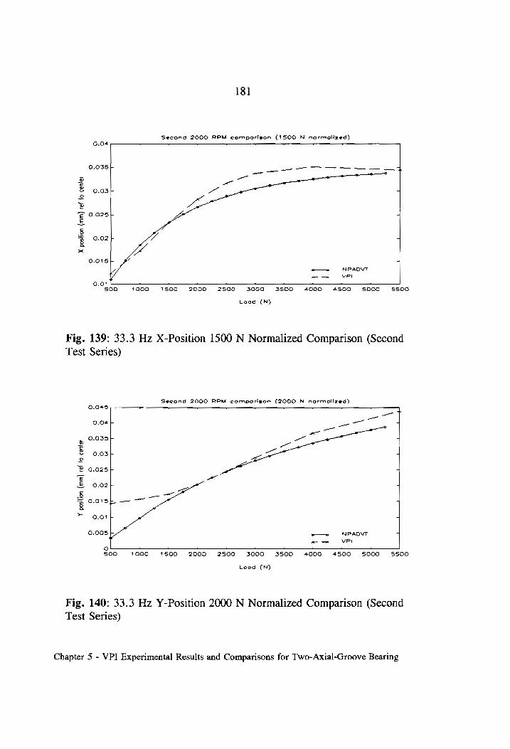
181

r T —r

Second 2000 RPM comporison (1500 N normolized)

oo NPADVT

—_— VPI

0.04

0.0355

2 & S 9.03F £

s “‘E 90.025>

a 5 B a.02}

x

O.0tS-

KG

q

0.01 500 19000 1500 2000 2500 3000 3500 4080 45900 5000 5500

Lood (NJ

Fig. 139: 33.3 Hz X-Position 1500 N Normalized Comparison (Second Test Series)


0.0445

0.04 -

0.0355

oO o

go 9°

o NO

Ss uo T

T

Y po

sili

on (mm)

tef

to center

Oo ° uv

o—o NPADVT “]

—_— VPI

Fig. 140:

o 0 1000 1500 2000 2500 3000 3500 4000 4500 5000 5500

Lood (N33



182

Second 3500 RPM comporison ( os token)

0.0355

0.03

0.025

0.02

0.015

X po

siti

on (mm)

ref

to center

Lo "SD

—_—

NPADVT

VPI

o §00 1000 4 500 2000 2596 3009 3500 49000

Lood (N}

4500 5000


Second 3500 RPM comporison ( os taken)

5500

0.05

0.025

0.92

0.015

0.01

posi

tion

(mm)

ref

to ce

nter

9.005

—-O.01-F

oe —

——

a ——

_— a

a _—

— o_o

_-*/

NPADVT

VPI

—

1000 -—9.015

500 1500 2000 2500 3000 3500 4000

Lood (N3

4500 5000


5500


183


0.035 r T r — —r-

0.034 |

®

& 0.025+ 4 £

Bb FE a.02+ 4 =

S * 0O.015- 7

S ZO >» YY“

0.01 1

— NBPADVT

-_—« VPI 0.005

S00 190090 1500 2000 25900 30006 3500 49000 45900 5000 5500

Lood (N)

Fig. 143: 58.3 Hz - Position, 1500 N Normalized (Second Test Series)

Second 3500 RPM comporison (2000 N normolized) 0.034 tT T r — r

0.03 4

0.025

O.ag-e a 4

0.015

9.01 a“

Y po

siti

on (mm)

ref

to ce

nter

0.005 - o—o NPADVT _—— VPI ©

500 190090 1500 2000 2500 3000 3500 4000 4500 5000 5500

Lood (N)

Fig. 144: 58.3 Hz Y-Position, 2000 N Normalized (Second Test Series)


184

Second 5000 RPM cornporison ( os token)

0.03 ~ . . . r — r

0.025+ ® = Q oe

[=]

= o.02F 2» = E = g 0.015+

g a

ot

0.01F

fo oo NPAOVT

——*« VPI

0.005 500 1000 1500 2000 2500 3000 3500 4000 4500 5000 5500

Load (N53


Second 5000 RPM campeorison ( of taken) 0.03 —- —

0.025

0.02

© © ui

6.01

0.005

Go

posi

lion

{m

m)

ref

to center

0.005

—-0.01 —— =o NPADVT

_——K VPI | —-90,.015

500 19000 1500 2000 2500 3000 3500 4000 4500 5000 5500

Lood (NJ)



185

Second S000 RPM cormmpcrisen (2000 N normolized)

0.03 = .

0.025 > = Y we

eo

~ O.02F v _

E £ 5 0.015 4 =

Qo a

><

0.01] 4

=o NPAOVT

4 — VPI

0.005 500 1000 1500 2000 2500 3000 3500 4000 4500 5000 5500

Leod (N)

Fig. 147: 83.3 Hz X-Position 2000 N Normalized Comparison (Second

Test Series)

Second SOOO RPM comporizon (2000 N normolized)

—— Tm

0.035

0.025

0.02

0.018

0.01

Y po

siti

on (mm)

ref

to center

0.005

——<—F

o S00

-——o NPAOVT

—_ VPI

19006 15090 2000 25900 3000 3500 4060 4500 5000 5500

Lood (Nj)

Fig. 148: 83.3 Hz Y-Position 2000 N Normalized Comparison (Second Test Series)

Chapter 5 - VP] Experimental Results and Comparisons for Two-Axial-Groove Bearing

186

5.5.8 Discussion for Comparisons to NPADVT

16.7 Hz:

33.3 Hz:

Chapter 5 -

For both tests, the x-position zero compares well. In general

though, the NPADVT analysis, although close, does not exhibit the

correct shape (this trend is the same as seen in the previous

comparisons to published results). The y-position results are quite

comparable with regards to the shape, except at light loads, where

the experimental y-position exhibits a peculiar flatness. It is possible

that this odd behavior is related to sleeve non-concentricity, as the

thermal effects for light loads at this speed should be minimal.

Surprisingly, the y-zero positions (as taken) exhibit fairly good

agreement between the analytical and experimental results.

For this speed, the x-position zeros show very good agreement

between analysis and experiment; the y-position zeros do not show

as good agreement. The x-position at low loads also shows good

agreement. As noted in previous comparisons to experiment,

though, while the sign of the slope of the experimental locus

changes, the analytical curve does not reflect this trend. The y-

position locus again shows good agreement, except at light loads,

where the experimental locus is oddly flat. The NPADVT analysis

VPI Experimental Results and Comparisons for Two-Axial-Groove Bearing

58.3 Hz:

83.3 Hz:

Chapter 5 -

187

is generally biased towards underestimating load capacity (the

analytical eccentricity ratio would be too large)

As with the previous data sets, the x-position zeros show generally

good agreement, while the experimental y-position zero is rather

different from the NPADVT result. The normalized locus curves

show good agreement between analysis and experiment. As before,

however, the experimental x-locus hints at a slope reversal not seen

in the analysis, and the experimental y-locus exhibits the unusual

flattening at low loads. The x-locus slope reversal is not as apparent

as in the previous two speeds due to the increased bearing load

capacity related to the increase in speed.

For this speed, the x-position zero shows good agreement between

analysis and experiment in the second test series, but not as good

agreement in the first. The y-position zero does not show good

agreement. In both the x-position and y-position shaft locus plots,

the analytical and experimental shape show some agreement, but not

as good as in previous cases. Part of the disagreement may be the

results of the experimental outliers discussed previously; however,

this effect does not explain all of the disagreement. The y-position

curve flatness is again seen for light loads. This flattening occurs

VPI Experimental Results and Comparisons for Two-Axial-Groove Bearing

188

for a greater range of loads, as would be expected for the increase in

load capacity caused by the increase in speed. As before, the

NPADVT results are biased towards a reduced load capacity; this

could be, in part, caused by the effects for variable clearances.

5.6 Comments and Discussion

This set of experimental data, and the comparisons between experiments and

between experiment and analysis, suggest that the test rig is basically

functioning correctly. Ignoring the zero position fluctuations, the data is

reasonably repeatable, although there is room for improvement. The

comparisons between the NPADVT analysis and experiment also show the

same general trends, i.e., agreement in Y, disagreement in X, as seen in the

comparisons to accepted published data. Thus the rig is not grossly altering

the bearing characteristics. Interestingly, Ref. 20, which is an analytical

examination of thermally induced bearing deformation, shows the same trends

as observed in these comparisons. In this work, it is shown that an analysis

which ignores thermally induced deformation tends to predict too large an

operating eccentricity; this is the trend observed in the comparisons between

NPADVT and the VPI rig. It seems unlikely that the strange flattening of the

locus curves seen at low loads are the results of thermal effects, as the


189

temperatures associated with light loads are correspondingly small. It is more

likely that this anomaly is related to shaft non-concentricity.

The biggest test rig problem appears to be the zero fluctuations. It seems most

likely that these are the result of effects external to the bearing/shaft interface

since the normalized data show such good agreement. The relatively close

agreement between most of the analytical and experimental x-position zeros

suggests that the problem is worst with respect to the y-position measurements.

This observation indicates that much of the problem may be related to thermal

growth of the large stainless steel bearing housing which is free to expand

symmetrically in the X direction, but constrained to expand only upwards in

the Y direction. There is also some experimental support for this hypothesis;

the housing vertical thermal growth has been measured to be between 0.051

and 0.102 mm when warmed from the lab ambient temperature of 18°C to

Operating temperature. The actual housing temperature probably ranges from

the nominal oil temperature of 43°C to something slightly lower, depending on

the operating conditions. The possibility of bearing thermal growth also

cannot be ruled out, as the clearance check/zero procedure takes about two

minutes; indeed, after one of the 83.3 Hz tests, the procedure failed a built in

settling check (the shaft resting position also noticeably changed as viewed on


190

an oscilloscope connected to a pair of the inner displacement probes). The

thermal growth issue also makes precise shaft alignment difficult. It is also

quite likely that some of the discrepancy is due to the fact that the lift check is

taken with the shaft stationary, and thus the run-out compensation values are

not applied. This fact could introduce an offset that could explain some of the

observed zero offsets.

Another effect which may have some impact is shaft bending. At full load,

there is a significant difference between displacement measurements at the

inner and outer faces of the bearing. Although the measured slope (relative to

the 1000 N zero position) is on the order of hundredths of a degree, the

absolute difference between the inner and outer measurements is a large

percentage of the bearing clearance. The exact effect of this deflection is not

apparent, but it does seem likely that it has some impact on the results. The

deflection also causes problems with the zero/clearance procedure; the applied

load must be large enough to firmly seat the shaft, but not so large as to cause

bending; the 1000 N load used was selected from only heuristic arguments,

and may not be the optimal load.


191

Other discussion, particularly concerning NPADVT, will be reserved for the

conclusions to this work.


Chapter 6

VPI Results and Comparisons for Pocket Bearing

6.1 Introduction

With the VPI rig shown to be functional within certain limits, it 1s of interest to

examine experimental data for a slightly different bearing geometry. Thus, the final

experimental data set examined in this work is for the 101.1 mm bearing described in

chapter 5 modified by machining a pocket into the upper half (see Fig. 2). The

interest in testing a pocket bearing is that one easy method of enhancing the stability

of a machine operating on a plain axial-groove bearing is to remove the bearing,

machine a pocket into the top of the bearing, and reinstall the bearing. This is

essentially the procedure followed with the VPI bearing. Thus, the results for the

modified bearing should be representative of the changes expected from this

modification. It turns out that the results for this bearing also exhibit some interesting

192

193

trends that may be construed as supporting the thermally induced deformation

hypothesis of the previous chapter. Data for this type of bearing are also not

available in the published literature. The test results presented in this chapter are for:

1) an initial three tests at speeds of 16.7, 33.3, and 58.3 Hz, and 2) a repeat of these

three tests. Loads of 500, 1000, 1500, 2000, 2500, 3000, 4000 and 5500 N are

examined. The 83.3 Hz speed employed in the previous chapter could not be attained

with the modified bearing due to problems with entrained air in the oil (a pocket

bearing has higher flow requirements than a plain bearing - the higher flow

overwhelmed the settling tank’s entrained air removal capability). The data as

recorded, as comparisons between the original and repeated tests, and as comparisons

between NPADVT and the experimental data, are presented. Comparisons will also

be made between the experimental and analytical shaft loci for the original bearing

and the modified bearing.

6.2 Pocket Bearing and Oil

The bearing for this test series is the original two-axial-groove bearing described in

chapter five, modified by the addition of a single pocket in the upper third of the

bearing. The modified bearing has the following characteristics:

Diameter: 101.6 mm

Chapter 6 - VPI Results and Comparisons for Pocket Bearing

Length:

C,/D Ratio:

Pocket Extent:

Pocket Depth:

Pocket Width:

Weep Hole Dia:

Oil Inlet Dia:

Feed Grooves:

194

57.15 mm

0.00160 to 0.00168

0 to 110 degrees from horizontal (CCW, against

rotation)

0.254 mm

42.93 mm (Centered in bearing)

1.6 mm

6.76 mm

OQ and 180 degrees from horizontal


2.5 mm maximum depth

The pocket to bearing surface transition at the 110 degree position is essentially as left

by the milling cutter, with only minor blending of the edge. As described in the

previous chapter, the bearing is of babbitt faced (0.43 mm thick), single piece bronze

construction, 139.7 mm O.D. The 203.2 mm O.D. horizontally split bearing holder

which adapts the bearing to the test rig bearing cavity is fabricated from 1018 steel.

It is the same width as the bearing. The bearing to holder fit is approximately line to

line. The fabricator’s inspection of the bearing and holder suggests that there should


195

be minimal distortion of the bearing bush caused by installation in the holder. The

bearing/holder assembly is installed in the test rig as discussed in chapter 3.

The oil used for this test series is the same ISO 32 oil used previously. For

reference, the properties of this oil and nominal inlet conditions are repeated below:

Density: 863 kg/m? at 50° C

Specific Heat: 1.98 kJ/kg*K at 50 °C

Viscosity: 16.1 mPaes at 40 °C 24.8 mPa®s at 50 ° C

Inlet Temp: 43 °C

Inlet Pressure: 0.034 MPa

Inlet flow rate: 0.7 to 0.8 cm/s

6.3 Experimental Procedure

The tests are conducted as described previously for the plain two-axial-groove bearing

tests (see chapter 5).


196

6.4 Experimental Pocket Bearing Data and Comparisons

The data for this bearing will be presented as recorded as well as for comparisons

between repeated tests, and a comparison will be made between the unmodified and

modified bearings.

6.4.1 Data

The experimental data for the pocket bearing, as obtained with the VPI rig, are

presented below in Fig. 149 through Fig. 154. These data are plotted for absolute

shaft position (X and Y) as offset by the bearing center coordinates as determined by

the post test lift check. The clearance obtained with this lift check is also included

with each plot. The estimated bearing center is to the upper left of these plots. Each

plot consists of the five measured points for each load at a given speed, as well as an

average shaft centerline curve. This average centerline curve is used in the

comparisons to NPADVT analysis, and is generated by finding the average X and

average Y coordinate for each group of five points.


197

19920111,n09 — 1000 RPM —-0.02 T T T T

—-0.025 L >

-0.03F _

2—0.035+ 4 i=

Db

oO © —O0.04F 0 o Data 4

‘wD 0.0454 — Avg. 4 E

= _o.osb 4 an o

%O.055-+ 7 >

-~O.06-+ =

—-0.065F- 5

-—90.07 ‘ . ‘ . —-90.06 -60.05 —-0.04 —0.03 —0.02 -0.01



19920118.p07 — 2000 RPM 0 T T T 7

~O.005}+ 5

-O0.01F+ ° 4

o 0.015 ~ 7

DD o © -0.02} 3 4 ‘D J-90.025+ eo oe Date 4

E E a,

— -0.03F+ — Avg. 7

wn oO

%O.035+ = >

-O.04+ -

—-O0.045+ 7

-—0.05 ‘ . . . —-0.06 —-0.05 —0.04 —0.03 -0.02 -0.01




198

19920119.nh35 — 3500 RPM

0.01 1 ' ,

0O,005F- ~

ol °

S0,005+ 4 i=

Db oO © —9.01F +

wD 270.015 + eo o Data 4

E

£ —-O.02- — Avg. 4

“a oOo

o&O.025+ 5 >»

-O0.03F+ 4

—-O.035F 4

-—0.04 ‘ " . . -—0.06 —0.05 —-0.04 —D.03 -0.02 -0.01



19920119.j52 — 1000 RPM

-—0.02 T T 7 T

—0.025F}+ -

-O.03F ~

3® 0.035 4 cc

Q

o 2 —-0.04+ 4

za Z-0.045+ co o Data 4

Ee

£ ~O.05-+ — Avg. 5

wn ©

&O.055+ 7 >

~O.06+ 1

-—-0.065- 4

—0.07 — . . . —0.06 ~0.05 —0.04 —-0.03 —0.02 —-0.01




199

19920119.m50 — 2000 RPM —0.005 T T ~T T

—O.01F

—0.015

-9.025-

0.025

—-O.03F- eo so Dato

mm)

ref

to ce

nter

Avg.

0s.

( o Gr wn

t |

oO —O.04 >

—0.045/

—O6.05- -—0.055 : : : 4

— 0.06 —-0.05 —0.04 —0.03 —0.02



19920119.p13 — 3500 RPM

—0.01

0 T OF T ¥

—90.005F

—O.01-

° QO _ wi T

—O.02+

ref

to ce

nter

0.025+ co o Data —

mm

= -0.03+ — Avg.

os

-0.04

—0.045- -0.05 , , ,

—0.06 -—0.05 —0.04 -—0.03 —0.02




-0.01

200


The data presented in Fig. 149 through Fig. 154 show a smaller, but similar, level of

scatter than the data presented in Chapter 5. The small magnitudes of the

experimental scatter lends support to the idea that the rig is basically functional.

Indeed, in the case of Fig. 153, the scatter is all but negligible. The outliers seen in

the remaining figures are again from the first set of 8 load points. This consistent

outlier behavior suggests that the mechanism causing the aberrant behavior is not tied

to the bearing geometry. The behavior seen in these plots tends to support the

thermal transient hypothesis, especially Fig. 152, which corresponds to 16.7 Hz data

taken during a test which began as an 83.3 Hz test, and became a 16.7 Hz test after

air bubbles were observed in the oil feedline. The entrained air does not explain the

observed behavior, as the rig was operated at low load at 16.7 Hz for a sufficient

time for the air to be eliminated, but possibly not long enough to achieve a new

thermal equilibrium. In all other cases, except the initial 16.7 Hz test of Fig. 149,

the rig was operated at the maximum load of 5500 N for approximately 10 minutes

before the autoloading sequence was initiated.


201

6.4.3 Comparisons For Repeated Tests

In Fig. 156 through Fig. 160, the three initial tests are compared with repeat tests for

the same nominal conditions. Due to the problem with zero position fluctuations, the

data are presented as recorded, as well as normalized at 5500 N. In the 5500 N

normalized plots, areas corresponding to plus or minus two standard deviations about

the mean of each group of four points are indicated for each load. See appendix B

for further details on these elliptical areas. Note also that the first (increasing load) 8

data points were eliminated from the data for these comparisons, since they seem to

reflect some thermal effect rather than normal experimental scatter.


202

Comparison for 1000 RPM repeated Pocket (as taken)

—0.02 T T T

—0.025+ 4

—O.03+ 4

09.0354 4 c @®

o

2 -0.04- oo First Run i

& l Wo 0455 ~-—-* Second Run 4

E l ££ _o.o5b 4 a g | RB o.055/ | 4

—~O.06+ | 4 +

—O0.065+ \ 4

\ —0.07 . . . .

~0.06 —0.05 -0.04 —0.03 —0.02 —0.01


Fig. 155: 16.7 Hz Repeated Tests (as Recorded)

Camparisan far 1000 RPM repeated pocket (5500 N norm) ~0.02 T T T T

/ 4

-—-09.03 L 4

—

—0.025

te Oo Oo Gl an T t

Oo

Oo

ul

uw T

Y pos. (m

m)

ref

to ce

n

— First Run 4 o 0 oO —_

——

—0.065 —- Second Run 4 ~0.07 , ! ,

—0.05 —0.04 —0.03 —0.02 -0.01 0


Fig. 156: 16.7 Hz Repeated Tests (5500 N Normalized)


203

Comparison for 2000 RPM repeated Pocket (as taken) 0 q FE T T

I © O +

|

|

| ° oO —_ ui '

eo First Run 4 | ° oO N un 5

= « Second Run -

-—0.045F-

-0.05 ;

—90.06 —©6.05 —0.04 —0.03 —0.02 -0.01



Comporigon for 2000 RPM repeated pocket (5500 N norm)

0 T T 4 qT

| O Oo

Bho T 1

| Oo oO

LA T i

Oo oO W

(@1) T i

Y po

s.

(mm)

ref

to center

—0.04 — First Run 4 T

——~

—-0.045F- { —- Second Run 4 L. —O0.05 : : ‘

—90.05 —0.04 —9.03 ~0,02 —0.01 ©


Fig. 158: 33.3 Hz Repeated Tests (S500 N Normalized)


204

Comparison for 3500 RPM repeated Pocket fas taken) 0.005 T T t T

of :

-0.005

—0.01}+

0.015-

os.

(mm)

ref

t9

center

e—e First Run _

wn Second Run _

—0.04+ 1 —0.045 m . ‘ ‘

~-~0.06 -0.05 —06.04 -—0.03 —0.02 —0.01



Comparison for 3500 RPM repeoted pocket (5500 N norm)

0.01 T t T qT

O.005F+ 4

OF =

a.005-+ = c wv

Oo

2 —-O.01F 4

© [-0.015+ 4 E

= —-O.02F- +

“a °°

&-O.025+ 4

-—O0.03F- — First Run 4

—-0.035F+ —- Second Run 4

—0.04 , , , -—0.05 —0.04 -—0.03 -—0.02 -—0.01 0


Fig. 160: 58.3 Hz Repeated Tests (5500 N Normalized)


205

6.4.4 Discussion of Repeated Tests

16.7 Hz:

33.3 Hz:

58.3 Hz:

The results for this speed show very good reproducibility; the

difference in zero is only slightly greater than the experimental scatter,

and the normalized comparison shows that the locus shapes are almost

identical. The plus or minus two standard deviation areas are contained

within the same area or touching, thus indicating good agreement.

The results for this speed are phenomenally good. Even in the non-

normalized plot, the curves are almost identical in both location and

shape. In the normalized plots, the two curves are seen to be all but

indistinguishable. This agreement is amazing, especially considering

the amount of scatter observed in the first test at this speed. The effect

of this scatter is evident in the different sizes of the areas corresponding

to plus or minus two standard deviations for the two curves.

The results for this speed show a much larger zero position difference

than do the previous two speeds. The normalized results, however,

again show extremely good agreement in the shapes of the two locus

curves despite the scatter observed in the first data set.


206

6.4.5 Comparisons Between NPADVT and VPI for Pocket Bearing

Comparisons between the experimental data and the NPADVT analysis for the same

nominal conditions are presented in Fig. 161 through Fig. 180. As with the

comparisons for the two-axial-groove bearing, comparisons to the actual data, as well

aS normalized comparisons, are presented. The normalized comparisons, however,

will not be presented for the second 33.3 Hz and 58.3 Hz tests since the resulting

plots would yield no new insight (the normalized plots for these two tests would be

the same as the normalized plots for the same speeds for the first test series since the

curves from the initial test and the repeat test are indistinguishable when normalized).

As with the two-axial-groove results, these plots include data for all five repetitions of

each load/speed point in generating the average centerline position. The data are

plotted as absolute shaft position relative to the bearing center versus load. The

NPADVT data is dimensionalized by multiplying the non-dimensional analytical result

by the appropriate clearance.


207

Comporison for first 1000 rpm

0.046 s . —_——_ Oe —_— TO

~~ O.044- a |

a

0.042 “ 7

& a = oD

oe > o*—\—-4 2 4

S — 7

£

£ 4

g a =

0.0284 o—a NPADVT -

— a VPI

0.026 1 2 : 2 . i . . . 500 1000 1500 2000 2500 3000 3500 4000 4500 5000 3500

Load (N)

Fig. 161: 16.7 Hz Pocket X-Position Comparison (First Test Series)

Comporison for first 1000 rpm

Y pos.

(mm)

ref

to ce

nter

NPADVT

— VPI

oO

0.015 S00 1000 100 2000 2500 3000 3500 4000 4500 5000 S500

Load (NS

Fig. 162: 16.7 Hz Pocket Y-Position Comparison (First Test Series)


208

Compcrison for first 1000 rpm ~ 1500 N norm

0.04

0.038

0.036 Fr

6.034

90.032

X pos

. (m

m)

ref

fo center

oO NPADVT a

a

VPI

0.026 S00 7000 1500 2000 2500 3000 3500 4000 4500 S000 3500

Lood (N)

Fig. 163: 16.7 Hz Pocket X-Position 1500 N Normalized Comparison (First Test

Series)

Comporison for first 1000 rpm — 1500 N norm

aoa NPADVT 4

— —- VPI

et

1000 1500 2000 2500 3000 3500 4000 4500 3000 3500

Lood (N)

Fig. 164: 16.7 Hz Pocket Y-Position 1500 N Normalized Comparison (First Test

Series)


209

Comparison for first 2000 rpm 0.05 r r . 7 r s — —

0.045

0.04

ef

lo center

= 0.035

0.03

X pos

. (mm

0.625 |

o—o NPADVT

a VPI tb.

0.02 , , ; 2 . 500 1000 1500 2000 2500 3000 3500 4000 4500 5000 5500

Lood ¢(N)


Cormporison for first 2000 rpm 0.05 7 7 r r r 7 a

0.045

0.04

° ° ul a

Y po

s. (mm)

ref

to center

0.01 5 o—a NPADVT

“ ——. VPI i

500 1000 1500 2000 2500 3000 3500 4000 43500 5000 5500

—t.

Load ¢N)>



210

Comporison for first 2000 rpm — 1500 N norm

0.038 —- r r r . r

0O.036F

Z 0.0344 = @

eo

o

~ 0.0325

2

‘€ € DOB F

a o a »~ 9.028F 4

0.0264 | o—o NPADVT

i, a on VPI 0.024 . 1 . 1 . . 1 _ :

500 1000 1500 2000 2500 3000 3500 4000 4500 50900 5500

Lood (N)


Series)

Comparison for first 2000 rpm — 1500 N norm

0.05 _— + r — r r +

O.045 5

0.04

e | € a ¥ 0.035 2

s = 0.034 €

& a ©O.025F+

Q a

~ 9.02 4

9.015) o——a NPADVT 7

4 — VPI

0.01 : : : —t : : : — : 500 1000 1500 2000 2300 3000 3500 4000 43500 S000 5500

Lood (N)


Series)


211

Comparison for first 3500 rpm

0.045

0.04

0.035 |

2 © o

X pos. (m

m)

ref

to ce

nter

§ o—ao NPADVT ——- VP en ———. ——t ——t

0.02 , , , — 500 1000 1500 2000 2500 3000 3500 4000 4500 5000 5506

Lood (N)


Comporison for first 3500 rpm 0.035 a ~ —— r 7 r r

0.03

0.025

9.02

9.015

0.01 Y pos. (mm)

ref

to center

0.005 + a a—o NPADVT

| _— VPI el nh.

Oo 4 4, 1 1 1 1 —L

500 1600 15090 2000 2500 3000 3500 4000 4500 S006 5500

Lood (N)



212

5500

Comporison for first 3500 rpm — 1500 N norm 0.036 . —— r = s r 7

0.0345

& O.O32F ca D S& 2 ~ O.03F

2 oo

= £ 0.028

os rad a

~ 8.0265 4

0.024) 4 q oo NPADVT

— wm VPI

0.022 . " n — . n 1 1 . 500 1000 1500 2000 2500 3000 3500 4000 4500 5000

Load (N)>


$500

Series)

Comparison for first 3500 rpm — 1500 N norm

0.045 7 — . ; r s

O.04F

& 0.035+ < a a °o = 0.034 2

E O.025 5

n

a

0.015 a 4 a“ ea—e NPADVT

a —— VPI 0.01 . . . — . . . — 2

500 1000 1500 2000 2500 3000 3500 4000 4500 5000

Lood (N)


Series)


213

Comparison for Second 1800 RPM

0.05 : 7 + r —-

par Pim eer le Teo oC ee

——

a“ — 0.0456 4 ral

a = “ x pA 2 O.04F 4 o —o—__#-—___¢

—

E ~~ 0.035 _

go | a bod

C.03F 4

4 a—o NPAOVT

— — VPI

0.025 4 : ; — 1 ; : : . 500 1000 1500 2000 2500 3000 3500 4000 43500 5000 5500

Load (N)

Fig. 173: 16.7 Hz Pocket X-Position Comparison (Second Test Series)

Cornporison for Second 1000 RPM

0.07

0.06

& 5 0.05 e

2

= = 0.04 £ e —

3 0.03

>

0.02

oa NPADVT

~—_——« VPI

0.01 . ‘ ‘ . ‘ — . . ‘ 500 1000 1500 2000 2500 3000 3500 4000 4500 5000 5500

Load ¢N)

Fig. 174: 16.7 Hz Pocket Y-Position Comparison (Second Test Series)


214

Second 10060 RPM — 1500 N norm

6.04 — r —

0.038

0.036

0.034

0.032

X pos. (m

m)

ref.

to ce

nter

NRPADVT

VPI

a—o

— —m

1600 1500 2000 2500 3000 3500 4000

Load (N)>

4300 3000 5500

Fig. 175: 16.7 Hz Pocket X-Position 1500 N Normalized Comparison (Second

Test Series)

$500

Second 10060 RPM — 1500 N norm 6.065 + r 7 r a r r

O.06F+

O.055-

& = O.O5F- a G 2 0-045 P

‘D> -~ 0.046

E ~— O.O35F a

a 0.03 4 >

0.025 4

0.02 o—\_<o NPADVT 4

— VPI

0.015 . . . . . 1 1 r 1 500 1000 1500 2000 2500 3000 3500 4000 4500 5000

Load (N)

Fig. 176: 16.7 Hz Pocket Y-Position 1500 N Normalized Comparison (Second Test Series)


215

Second 2000 RPM

0.05 - = : . + . ~

0.045; eee —_—_ ~~

a —_— s _ a

YQ

2 0.04F a , = a“ ;

<= “ = o.035f 4 o oa =a

=

0.034 4

a——o NPADVT

—_—_— VPI

0.025 — . . ‘ . — ‘ ‘ 500 1000 1500 2000 2500 3000 3500 4000 4500 5000 5500

Load (NJ


Secand 2000 RPM

0.05 . : r

0.045

0.04 & cc a

¥ 9.035 2

@ = 0.03 E

£ - 0.025

a

&

~ 9.02

0.015% oa a—ao NPADVT L — VPI

0.01 —__ — —

S00 1000 1500 2000 2500 3000 3500 4000 4500 3000 5500

Load (N)



X pos

. (m

m)

ref.

to ce

nter

216

Second 3500 RPM

0.042 o

— oon —*s

0.044 _a a a ~

0.0384 a“ 4

a — 0.036 ~ 4 “

0.034 a a 7

0.0325 +

O.O3F 4

0.028 F 4

©O.026F 4

0.024 F- o®—a NPADVT 4

a VPI

0.022 . : ‘ : : ° 1900 2000 3000 4000 5000 6000

Load (N)


Y po

s. (mm)

ref

to center

Secand 3500 RPM

0.04

0.035

0.03

© o n ul

0.02

2 6 a

0.01

a—o NPADVT

1 —_—- VPI 0.005 , ! -

SOO 1000 15090 2000 2500 3000 3500 4000 4500 5000 5500

Lood (N)



217

6.4.6 Discussion of NPADVT vs. VPI for Pocket Bearing

16.7 Hz:

33.3 Hz:

Both of the comparisons for this speed exhibit a large x-position zero

offset; the y-position zero in general looks quite good. This result

tends to cast some doubt on the earlier hypothesis that the thermal

effects primarily cause offsets in the y-position measurements. The x-

position shaft locus also shows generally good agreement for the

normalized plots, with increasing deviation as the load increases. This

deviation may be, in part, caused by shaft bending and thermal effects.

Interestingly though, for this bearing, the NPADVT results hint at the

same slope sign reversal as the experimental data. The analytical and

experimental y-position shaft locus also show a great deal of

agreement, again deviating smoothly as load increases. Some portion

of this disagreement may be related to shaft deflection; this point will

be discussed in the conclusions to this chapter.

As with the 16.7 Hz data, the x-position zero in the actual data plot is

considerably worse than the y-position zero, which shows fairly good

agreement. The normalized plots also compare favorably. Again, the

analytical x-positions are larger than those seen in the experimental


218

data, and the analytical y-positions are smaller than the experimental

coordinates for larger loads (for normalized data).

58.3 Hz: The data for this speed repeat some of the trends observed earlier. The

general shapes of the curves are very similar, with the analytical x-

positions generally larger than experiment and the analytical y-positions

generally smaller than the experimental values for large loads (in the

normalized plots). The comparison of zero positions does not show as

good agreement as before.

6.4.7 Comparison Between Pocket and Plain Bearing

To illustrate the alterations in shaft locus caused by the addition of a pocket to a plain

bearing, Fig. 181 and Fig. 182 present, respectively, the NPADVT analytical curves

and the experimental curves for 33.3 Hz. It should be noted that in both plots the

plain bearing’s clearance is slightly smaller than the pocket bearing’s clearance. The

plots are both in dimensional form. In the experimental data plot, areas for plus or

minus two standard deviations about the mean, based on the last four load repetitions,

are again indicated.


219

NPADVT Pocket vs Plain Comparison 26000 RPM

oO qT qT v F T

—0.005- 4

—0,01+ 4

za g- O.015- 7

oO

2 — —O.02F5 7 v

Ee L 7 E 0.025

8 _o.o3t a

>

— 08.035 fF i o—o Ploin Brg. (Cd = 0.157) 7

-0,04F5 £ = « Pocket Org. (Cd = 0.165) 7

—0.045 —0.04 —0.035 ~9.03 —0.025 —0.02 ~0.015 -0.01


Fig. 181: Comparison Between Plain and Pocket Bearings, 33.3 Hz (NPADVT)

Experimentol Comparison of Plain to Pocket Bearing

0.01 +

OF 4

s | a 4 & -0.01 >

= / g / = -o.0z+ 4 E i ~ t 8 _g.a3/ f 4 $ -0.

> f { __ Plain Brg. (Cd = 0.152 mm)

-0.04- 9 4 { —- Pocket rg. (Cd = 0.169 mm)

e

~0.05 , — , —0.04 ~0.03 —0.02 -0.01 Oo 0.01


Fig. 182: Comparison Between Pocket and Plain Bearings, 33.3 Hz (Experimental)


220

6.4.8 Comments on Bearing Type Comparison

Although Fig. 181 and Fig. 182 present a rather different view of the changes in shaft

locus caused by adding a pocket to a plain bearing, several observations can be made

(the differences are probably the result of both analysis problems and experimental

zero shifts). One observation is that in both cases the pocket does load the bearing

down and away from the pocket (i.e., towards negative X and Y for a pocket starting

at positive X and continuing counter-clockwise), as one would intuitively expect. It

may also be observed that the shift causes a reduction in the magnitude of the cross-

coupled stiffness (the locus curve is more nearly vertical for a given load), which

would have a stabilizing effect. The final observation is that the pocket causes some

reduction in load capacity/operating film thickness. The NPADVT analysis suggests

that the effect on ultimate load capacity is slight, as the decrease in film thickness

occurs primarily at light loads, and has less of an effect at higher loads, as one would

intuitively expect. The experimental results shown a much more pronounced curve

shift, although this shift may be in large part due to zero offsets and shaft deflection

effects.


221

6.4.9 Comments and Discussion for Pocket Bearing

In general, the results for this bearing geometry show reasonably good agreement,

especially with regard to slope. This agreement suggests that the stiffness values

obtained from NPADVT may be reasonably useful for this bearing. Interestingly the

NPADVT analysis shows a similar x-position slope sign reversal as seen in the

experimental data; this similarity differs considerably from the plain bearing

comparisons (the similarity is most apparent in the 16.7 Hz comparisons). Also, the

differences between the NPADVT analysis and the experimental data are opposite

those observed for the plain bearing (i.e., the NPADVT eccentricity is generally too

small). This could be construed as suggesting that the bearing loading induced by the

pocket overwhelms any thermally induced deformation effect. The comparisons

between the NPADVT analysis and the experimental data also suggest that shaft slope

may be causing a measurement error due to the systematic and smoothly increasing

difference between the curves. This hypothesis also receives support from the

observation that the difference between experimental data and the NPADVT analysis

at the maximum load is of almost the same magnitude in each of the normalized

comparisons. Based on these observations, an examination was made of the loading

effect on the measured displacements with the shaft stationary. After obtaining the

zero and clearance as in the experimental procedure, the shaft was loaded to each of


222

the experimental loads and the measured position was recorded. For the hypothesis

of a load dependent measurement error to be correct, basic beam theory would

indicate that an offset linearly dependent on applied load should be expected

(assuming a constant pivot, etc.). Although a position error of the correct sign was

observed and the relationship between the error and applied load was a smooth curve,

it was not linear. Thus, although the measurements seem to suggest that there is a

measurement error related to applied load, the exact mechanism is not simple shaft

deflection, and should be examined further before a correction equation is specified.

The possibility of some effect on the fluid/bearing interface as the result of shaft

bending also seems likely.


Chapter 7

Conclusions and Recommendations

7.1 Conclusions for NPADVT

As seen in chapter 4, NPADVT seems to model the fluid mechanics of a fluid-film

bearing in a sufficiently consistent fashion that it can be used as a yardstick for an

initial evaluation of the VPI rig. In general though, the program has a number of

shortcomings which need attention. NPADVT, although certainly a useful program,

cannot be considered a highly accurate design tool. The program does seem to

successfully capture the gross characteristics of a bearing, but misses many of the

important details. Most significant is the fact that it does not do a good job of

predicting the cross-coupled stiffness effect. This problem also casts doubt on the

cross-coupled damping coefficients. In addition to the problems with the cross-

coupled effects, other weaknesses include the lack of an option for user

223

224

spacing/placement of nodes, and the limit on the maximum number of nodes. These

weaknesses are especially evident in the difficulties with successfully modeling the

single groove bearing of Ref. 3. The analysis for this bearing also points out a

problem in the temperature-viscosity iteration procedure, as the temperatures would

sometimes start to diverge if too many temperature-viscosity iterations were

employed. A final problem is that NPADVT is not very user-friendly, relying on

formatted input and output files as a means of interacting with the user.

7.2 Conclusions for the VPI & SU Test Rig

From the comparisons between experimental data presented in chapters 5 and 6, it

would appear that the VPI rig generally functions in a consistent manner (ignoring the

zero offset problem). The data exhibit very good repeatability between repeated tests,

particularly considering that in some sense the test rig is still in the early phases of

debugging. The comparisons between VPI data and the NPADVT analyses show the

same trends and exhibit generally the same level of, or better, agreement between

NPADVT and experiment as do the comparisons in chapter 4 to the accepted

published data. Thus, using as criteria both internal consistency and agreement with a

calibrated external measure, it would seem reasonable to conclude that the VPI & SU

test rig can be considered useable. This designation of useable carries with it the

proviso that the rig still needs some work before it can be considered an operational,

Chapter 7 - Conclusions and Recommendations

225

precision test instrument. Suggestions for improvements and problem areas to be

examined will be discussed following the recommendations regarding NPADVT.

7.3 Recommendations for NPADVT

Although the primary thrust of this work was not an evaluation of NPADVT, an

appreciable amount of effort was expended in evaluating the program for use as a

measure of the VPI rig’s performance. Thus, the background for several

recommendations concerning the program’s analysis has been presented. Since the

primary motivation for having an analytical analysis of fluid-film bearings is the need

for dynamic bearing coefficients for use in a rotor dynamic analysis, the problems

with the cross-coupled term(s) seen in almost all of the comparisons are in the

greatest need of attention. The problem does not seem to be entirely related to the

simple thermal model in NPADVT; some of the other assumptions may need to be

questioned. The fact that the comparisons between analytical data and experimental

data in Ref. 18, which uses essentially the same assumptions as NPADVT but a more

complex thermal model, shows the same sort of disagreement with regards to the

cross-coupled effect supports the hypothesis that there is some important factor being

ignored in the analysis. One assumption that does not seem to have been examined at

great length in the literature is the assumption of no significant mechanical

deformation as the result of the film temperature gradients. There is a significant


226

temperature rise through the region of minimum film thickness; it would not seem too

unreasonable to suppose that this gradient could give rise to sufficient mechanical

deformation to alter the characteristics of the bearing. Although such deformation is

generally dismissed as negligibly small, the combination of a thin film and the

likelihood of very high bearing sensitivity to geometry changes in this region could

contradict this assumption. One of the few works that addresses the issue, Ref. 20,

presents analytical results which show changes in the static operating locus similar to

those observed in the comparisons of Chapters 4-6. Preliminary work to quantify this

effect is also currently underway at VPI & SU, and should be continued. The results

of this investigation should also be coupled to an NPADVT analysis. Depending on

the results of this work, some simple thermally induced mechanical deformation

model may need to be incorporated into NPADVT.

Although there 1s some analysis (Ref. 18) which suggests that the simple NPADVT

global energy balance is adequate, it would be useful to update NPADVT to include

local film-temperature and viscosity variations. This local modelling would also be

required if the results of the thermally induced deformation study show that there is a

significant effect. It might also be fruitful to investigate the possible time savings

resulting from going from the current two-layer solution approach of

1) approximate (closed form) solution,


227

2) full 2-D solution,

to a three level approach of:

1) approximate (closed form) solution

2) 1-D circumferential solution (assume an axial pressure profile as in

Ref. 14),

3) full 2-D solution.

The logic behind this approach would be that the majority of the time is used in

developing a good estimate of the shaft position, and a 1-D circumferential solution

would be considerably faster in developing a good estimate. The estimate could then

be refined by a more exact 2-D solution. It might also be helpful to include a better

treatment of the cavitated region of the bearing. Finally, some effort to increase user

friendliness and eliminate the occasional convergence problems with the temperature-

viscosity iteration step would be helpful.

7.4 Recommendations for Test Rig

The recommendations for test rig upgrades/improvements and detailed study can be

broken down into several general items:

1) Thermal Growth Effects

2) Other Misalignment Effects

3) Data Acquisition


228

4) Oil System

5) Speed Control and Miscellaneous Instrumentation

6) Rig Mechanical

7) Miscellaneous

Each of these items will be discussed separately below.

7.4.1 Thermal Growth Effects

The test rig seems to have some significant problems with thermal growth of

components. Not only does the bearing bush itself measurably change diameter from

warmed-up (i.e., at the oil inlet temperature) to operating conditions, but more

significantly, the bearing housing itself experiences a large (relative to the magnitude

of clearance and measurement accuracy) dimensional change between ambient and

operating temperature. There is also some variation in housing dimensions which is

correlated with operating load and speed. Since the rear support bearing does not

mirror these changes, this growth causes misalignment problems. The misalignment

effect alone is not too difficult to control; the rear support bearing could be readily

mounted on a pair of (large) lead-screws to enable it to be moved to accommodate

some misalignment. The problem is one of measurement. Unfortunately, it is

difficult to imagine a means of measuring the actual operating bearing dimensional

changes short of installing displacement probes in the test rig shaft. Although shaft


229

mounted probes have been employed (for examples, Ref. 18 or Ref. 30), the speed

range (up to 500+ Hz) of the VPI rig would cause problems from a materials

standpoint (centrifugal loading is extremely high at these elevated speeds), as well as

problems with passing the signal from the shaft (this speed range seems likely to

cause problems for slip-rings). The fact that the shaft would need to be bored to

bring the signal leads to the turbine end where slip rings could be mounted is also a

complicating factor. One simpler proposal for measuring the effects of the thermal

growth is to monitor the center-line height of both bearing housings relative to the rig

base and adjust the rear bearing housing height to match the thermal growth of the

test bearing housing. This approach would only work for vertical growth, but this is

probably the major housing growth effect. This approach will not help in reducing

the effect of bearing diametral growth, but perhaps a means of rapidly stopping the

rig and rapidly measuring the clearance can be devised. If taken rapidly enough, this

measurement should reflect the actual operating geometry.

Another approach to controlling misalignment effects is to mount a pair of pressure

transducers in the bearing, equidistant from the bearing centerline, and adjust the rear

shaft position until the indicated pressures are equal. This approach has the advantage

that shaft slope through the bearing caused by loading can also be reduced or

eliminated. If two sets of transducers are mounted with sufficient angular separation,


230

this approach should work for misalignment in both X and Y directions. This

approach, however, will only work for midplane symmetric bearings and requires the

installation of two to four pressure transducers. Although this approach seems to be a

very good solution to the misalignment problem, more study is warranted. The

installation of two more displacement probes at the bearing outer measurement

location would also be helpful, since dual probes would allow some of the effect of

the housing growth on the measurement to be cancelled out. It is also possible that

some form of active temperature control of the bearing housing could be of help in

reducing the amount of thermal growth correlated with different load and speed

conditions.

7.4.2 Other Misalignment Effects

In addition to the thermally induced misalignment, the applied shaft load introduces

measurable shaft bow, which effectively causes some degree of misalignment at the

bearing. Measuring this misalignment is not as great a problem as measuring thermal

growth effects, since a reference shaft slope can be obtained at low load with the shaft

Stationary and the loading induced slope can be measured relative to this reference

(this is presently done). Since this measurement is fairly easy to obtain, the larger

problem is to remove the misalignment. Manually moving the rear bearing carrier is

not a good option due to the mounting method, nor does moving the main bearing


231

housing seem to be a good idea. The most workable solution is, as suggested above,

the installation of a pair of lead-screws which can be remotely operated (probably

large studs with slightly different thread pitch on each end). If these lead-screws are

of large diameter (for high stiffness) and the pitch of the threads at the ends is close

(for fine adjustment), this approach would seem to be likely to work well. The

possibility of an improved method of obtaining the initial alignment also needs to be

investigated.

7.4.3 Data Acquisition

Although the current combination of stand-alone and PC-based instrumentation has

proved workable for the static testing conducted to this point, it will be extremely

difficult, if not impossible, to adapt it to dynamic coefficient identification. The

combination of a slow integrator for measuring the average shaft position coupled

with a separate 8-bit dynamic waveform measurement will not work very well for this

purpose. Even with static testing, there are some recurrent problems. These

problems include occasional communication glitches related to the fact that the stand-

alone instrument is not designed for complete computer control. The instrument also

has not proved to be an extremely reliable piece of equipment. The data transfer rate

from this instrument is also too slow for real time display. It is also difficult to

expand beyond the current 8 channel data acquisition capability. It seems most likely


232

that some combination of plug-in PC based instrumentation will be best suited to

future and present needs, although the possibility of IEEE 488 or other external

instrumentation should not be ruled out entirely. The future instrumentation needs

and specifications need to be developed and the hardware upgraded. A portion of this

upgrade will necessarily include a major software rewrite, which should be aimed at

maintaining as general-purpose a test environment as possible, with a reliable, user-

friendly interface.

Another data-acquisition problem that needs to be addressed is zero drift. The

problems with regard to the displacement measurements has been discussed

previously. The load measurement system also exhibits this problem. The effect is

most strongly seen in the up load cell, where the zero commonly shifts some 10 to 30

N over the course of a day of testing. This problem is not entirely the signal

conditioning, as similar drift is seen with a separate digital readout. It also is unlikely

that this drift is completely caused by sensor temperature sensitivity. The drift

mechanism needs to be identified and eliminated. The torque sensor, likewise, has a

problem maintaining a zero setting, but this may largely be a result of shifts in the

structure holding the air inlet to the air turbine. Zero drift in the temperature input

board needs to be addressed as well.


233

Another instrumentation problem is the lack of expansion capability. As mentioned

above, it would be helpful to add two more displacement probes to the outer

measurement location of the test bearing. With current instrumentation, this addition

would require eliminating the rear bearing measurements. Also, for dynamic

measurements, it will be necessary to simultaneously sample both load and

displacement measurements; this need will greatly increase the number of required

data input channels. The ability to obtain data in real time would also be required for

controlled excitation. It could also be helpful to have the option of adding load

measurement to the rear support bearing and/or to the test bearing. A redundant load

measurement obtained by measuring the magnet field strength could also have several

advantages.

The final instrumentation issue concerns load cell calibration. Currently the load cells

can only be calibrated in place via shunt calibration. It would be reassuring to

develop some means of providing dead-weight calibration for the load measurement

(even if this is not possible in-place, the availability of a method of providing a

precise dead-weight calibration up to about 7000 N would be helpful).


234

7.4.4 Oil System

The rig oil system currently has two major shortcomings: the temperature regulation

is not always as precise as desired, and the methods currently employed to eliminate

entrained air only work at very low flow rates. The control problem is mainly related

to the imbalance between the large oil cooler capacity and the small oil heating

capacity. This imbalance manifests itself when the temperature goes far below the

nominal setting by causing the recovery period to be extremely long. The proposed

solutions are a combination of:

1) further reductions in cooler capacity (this will most likely entail a new,

smaller cooler, as the current shell and tube cooler has already been

reduced to a fraction of its capacity by eliminating half of the passes

and blocking about half of the remaining tubes) and moving the cooler

closer to the bearing oil inlet to reduce the time lag between the cooler

and the controller sensor, and

2) adding more heater wattage.

If applied correctly, increased heater wattage could also aid in the removal of

entrained air by heating the drain oil, thereby reducing its viscosity, thus allowing air

bubbles to rise to the surface and release the air more rapidly. To improve the

entrained air removal rate, the size of the settling pan and/or the drain piping should


235

be increased to increase the exposed oil surface area. Other options may also need to

be explored.

7.4.5 Speed Control

Although the speed controller functioned adequately during the testing, it is far from

being operable by an arbitrary user. There are two basic problems. The first is a

problem with one or both of the software and/or signal conditioning which causes the

controller to occasionally lose track of the speed signal. This signal loss causes the

control valves to either both temporarily close (the recovery from this upset is usually

graceful), or to both go wide open (this usually is not so graceful; generally the rig

rapidly accelerates until the secondary controller closes the shut-down valve). This

problem needs to be remedied. It would also be beneficial if the fix includes a

redundant speed pick-up; if the current speed signal is lost due to sensor failure or

cabling problem, the control valves would both go wide open, but the secondary

controller would never provide the redundant shut-down capability. Most likely, the

bearing and/or rig would be damaged. This upgrade is currently being pursued, and

the hardware is on hand.


236

The second problem with the speed control system is that the small control valve is

too big for the degree of control precision required. This problem, in turn, requires

that the controller output changes be very small. These small control magnitudes

make the controller unnecessarily sensitive to control parameters, which must be

tweaked for different operating speeds to obtain the degree of speed control desired.

The ideal fix would be to replace this air-to-close (i.e., the value is fully open when

no control air pressure is applied) valve with a smaller air-to-open valve, thus

improving control as well as gaining a better failure mode. The alternative is to fit

the current valve with a reduced seat and valve stem. It would also be helpful to

characterize the non-linear transfer function between the magnitude of the control

valve control signal and the turbine output torque. An experimental determination of

this transfer function would not be too difficult for the case of a locked rotor. The

extension to running conditions could be made through use of the turbine operating

Curves.

Hardware on hand to allow the PC used for turbine control to also perform

temperature monitoring for the two turbine bearings and the rig rear support bearings

needs to be completed and installed. With this hardware, automatic monitoring of the

bearing temperatures will enable automatic shutdown to be provided for abnormal

temperatures. This hardware installation will ultimately include both warning as well


237

as trip settings. This monitoring capability also includes other rig temperatures, oil

level switches and the minimum oil pressure switch. Air compressor remote

condition monitoring could also be added (instrumentation would need to be added to

the compressor). Compressor condition monitoring would be fairly inexpensive, but

extremely beneficial.

7.4.6 Miscellaneous Instrumentation Upgrades

The current load cells have measurement uncertainties that could be improved upon,

especially with regards to hysteresis. New, lower capacity load cells will also

certainly be desired for dynamic load measurements of the magnitudes under

consideration (typically 10 to 20 percent of the current load capability). The ability to

provide an auxiliary load measurement through use of a magnetic field strength sensor

could also be advantageous. This measurement would not be affected by inertial

effects and could allow the magnitude of residual magnetism (and the resulting

residual load) to be quantified. For dynamic coefficient extraction, load measurement

at the test bearing will almost certainly be required. To eliminate inertial effects, the

test bearing acceleration would also need to be measured if load cells are installed at

this location. To reduce the problem of mass uncertainty in the inertial correction, it

would be desirable to develop a load measurement system that would allow the mass

of oil in the bearing to be ascertained. Any load measurement device at the test


238

bearing must also be extremely stiff, so as not to unduly affect the dynamic behavior

of the test rig.

Another useful instrumentation addition, albeit a very difficult addition, would be

shaft based instrumentation at the test bearing location. The problems discussed

previously make the successful installation of such instrumentation unlikely. Finally,

it could be helpful to have an accurate measurement of the bearing torque. This

measurement could be useful in comparisons to analyses. The most obvious method

of implementation is to mount the test bearing in a second, low friction bearing and

measure torque by measuring the restraining force required to hold the assembly in

place. The implementation of this approach could, however, be far more difficult

than the benefits would justify.

7.4.7 Rig Mechanical

There are two primary mechanical problems with the test rig: the shaft run-out

associated with the sleeve installation and the housing thermal growth. The thermal

growth issue has been discussed previously and will not be discussed further. With

regard to the sleeve run-out issue, although the use of shaft sleeves is appealing from

the viewpoint of test rig flexibility, it is difficult, if not impossible, to reliably install

a sleeve and maintain concentricity and parallelism on the order of 0.003 mm. The


239

best solution is to procure solid shafts of selected diameters. As most of the

anticipated experimental work would be with U.S. standard dimensioned bearings,

typical diameters of 4" and 2" would be good initial sizes. The current shaft could be

modified to one of these diameters; a second solid shaft would have to be fabricated

from scratch. Alternately, the current shaft could be retained as a backup, and two or

more new shafts fabricated. The change to a solid shaft would require some

modification of the current seal arrangement at the test bearing location, but this

should not be too costly. This change is one of the priorities indicated below.

Some examination should also be made of the possibility of replacing the current

duplex ball rear support bearing with a high pressure hydrostatic bearing. Although a

certain amount of expense would be involved, it would be partially offset by

eliminating the requirement to purchase a new set of bearings for new shafts. The

hydrostatic bearing would offer several other advantages: very long life, possibly

increased stiffness, increased damping, and potentially smoother operation (the current

duplex ball bearing exhibits rather wild looking run-out, which could increase the

noise level at the test bearing for dynamic measurements). The change to hydrostatic

operation could also include a high capacity thrust bearing. Thrust capacity would

become important for testing bearings such as the end fed damper seal (bearing) under

consideration for use in a Space-Shuttle main engine turbopump, or the possibility of


240

seal testing with the loading magnets operating as a magnetic bearing in addition to a

forcing input. This type of testing would most likely involve high pressure fluid

creating a large thrust load on the end of the shaft at the test bearing end.

Conventional bearings that can react high thrust loads at speeds of 500 Hz are quite

expensive. A possible drawback to the hydrostatic bearing(s) would be a potential

increase in the required drive power.

Finally, either the current right loading magnet needs to be mounted, or magnets

optimized for dynamic loading need to be fabricated and installed. Either addition

would allow arbitrary axis loading. One benefit of arbitrary loading is that the

clearance could be determined for the entire bearing by loading at a number of

angles. The ability to provide arbitrary loading could also be helpful in bearing

evaluation.

7.4.8 Miscellaneous Recommendations

A number of other needs and items to investigate have become apparent over the last

8 months of rig operation. These items will be listed below in no particular order.


241

> Air compressor spares should be obtained. The source could include

new parts, as well as acquisition of entire compressors to junk for

usable parts, or parts that can be reconditioned. A spare air

compressor would be an unlikely but even better option.

> Air turbine capacity reduction should be examined in detail. The

current turbine power output far exceeds requirements. A removable

reduction in the number of turbine nozzles could provide a useful level

of rig capability, while reducing the drive air requirements. It would

be helpful to be able to operate at reasonable speed and load from the

shop air system. Such operation is not presently possible, but the

turbine curves suggest this operation would be possible with a reduction

in the number of nozzles. This same investigation would also point the

way towards increasing drive power should this ever become needed

(more air compressor capacity would be required).

> Although the muffler currently on the turbine exhaust provides a

phenomenal degree of noise control, the noise is still objectionable for

long periods of exposure and/or high speeds and loads. It would be

desirable to construct a sound box around the muffler and the control

valves (which also generate a surprising amount of noise). This project


242

could also be coupled with ducting to exhaust the drive air to the

outside of the building.

> The loading control system needs to be upgraded; the current algorithm

is slow and not very sophisticated. Better alternatives can be easily

developed.

> Work needs to be done on the automation software to provide greater

flexibility in testing and to allow other users to operate the test rig.

These upgrades also tie in with the upgrades in condition monitoring.

The ability to accommodate pressure probes also needs to be added to

the data acquisition system.

> A knowledgeable lab technician would be very helpful. Not only could

a good technician take over some of the physical upkeep of the rig, but

such a person would also provide a greater degree of continuity

between successive graduate students working with the test rig.

Admittedly, such a person is difficult to find and retain.

7.4.9 Priorities

Since an array of possible rig improvements and items to examine has been presented

in this chapter, this concluding section will present a prioritized list of some these


243

items based on cost, time, and potential future requirements. The items will be

grouped as: Immediate, 1 Year, Long Term.


244

Table XII - Immediate Rig Improvement/Study Items

Immediate Items

Item Est. Cost Est. Time

Solid Shaft/Hydrostatic Brg. $2k - $5k weeks to months

Study and Acquisition (acquisition)

Find and Reduce Zero Drifts Low weeks

Add Pressure Probe Ability $300 + Probes days

Thermal Growth Study/Control | Unknown days to weeks

Improve Temperature Control Low + possible new days

cooler

Improve Speed Control Low days to weeks

Study Air Turbine Capacity Unknown days

Reduction

Examine Alignment Methods Low days


245

Table XIII - 1 Year Rig Improvement/Study Items

1 Year Items


Rear Bearing Running <$2k weeks

Adjustments

Entrained Air Removal low days to weeks

Improve Speed Control low days to weeks

Large Thrust Capacity $1k to <$10k weeks to months

Thermal Growth Control ? days to months

Shaft Deflection Control days to months

Dynamic Measurements ?? days to months

Calibration Upgrades <$1k days to weeks

Instrument Compressor < $500 days

Noise Control < $200 days

Software Improvements low months

Air Compressor Spares ? months

Instrumentation Upgrades $1k to ? months


246

Table XIV - Long Term Rig Improvement/Study Items

Long Term


Dynamic Measurements ? months

Instrumentation Upgrades ? months

Torque Measurement ? months

Software Improvements low months

Calibration Improvements ? weeks

Air Compressor Spares ? months


References

Allaire, P.E., Nicholas, J.C., Gunter, E.J., "Systems of Finite Elements for

Finite Bearings." J. of Lubr. Tech., Trans ASME. 98, 2, pp 187-197, 1977

Allan, T., "The Application of Finite Element Analysis to Hydrodynamic and Externally Pressurized Pocket Bearings." Wear. 19, pp 169-206, 1972

Andrisano, A.O., "An Experimental Investigation on the Rotating Journal Surface Temperature Distribution in a Full Circular Bearing." J. of Tribology,

110, pp 638-645, 1988

Booker, J.F., Huebner, K.H., “Application of Finite Element Methods to

Lubrication: An Engineering Approach." J. of Lubrication TechTechnology 24, 4, pp 313-323, 1972

Branagan, L.A., "Thermal Analysis of Fixed and Tilting Pad Journal Bearings

Including Cross-Film Viscosity Variations and Deformations.” PhD Dissertation, University of Virginia, Charlottesville, VA, 1988

Brockwell, "Measurements of Steady-State Operating Characteristics of a 5-

Shoe Tilting Pad Journal Bearing." Tribology Transactions, 32, pp 267-275, 1989

Coleman, H.W., Steele, W.G., Experimentation and Uncertainty Analysis for

Engineers, Wiley-Interscience, 1989

DeChoudbury, P., “A Comparison of Film Temperatures and Oil Discharge

Temperatures for Tilting Pad Journal Bearings." J. of Lubrication Technology, 103, pp 115-119, 1981

Ferron, J., Frene, J., "A Study of Thermo-Hydrodynamic Performance of a

Plain Journal Bearing, Comparison Between Theory and Experiement." J. of

Lubrication Technology, 105, pp 422-428, 1983

247

10.

11.

12.

13.

14,

15.

16.

17,

18.

19,

20.

248

Flack, R.D., Allaire, P., "An Experimental and Theoretical Examination of

the Static Characteristics of 3-Lobe Bearings." ASLE Trans., 25, pp 88-94,

1982

Heller, S., "Static and Dynamic Performance of Externally Pressurized Fluid Film Journal Bearings in the Turbulent Regime." J. of Lubrication

Technology, 96, pp 381-390, 1974

Hinton, "Characteristics of a Statically Loaded Journal Bearing with

Superlaminar Flow.” J. of Mechanical Engineering Science, 22, pp 79-94,

1980

Kirk, R.G., Input Instructions for Multi-Pad Fixed Bore Fluid Film Bearing

Analysis ----NPADVT----. VPI&SU Rotor Dynamics Lab Manual, January (1990)

Knight, J.D., Barrett, L.E., Cornan, R.D., "The Effects of Supply Pressure

on the Operating Characteristics of Two-Axial Groove Journal Bearings."

ASLE Trans. 28, pp 336-342, 1985

Leader, M.E., "Experimental Study of 3 Journal Bearings with a Flexible

Rotor." ASLE Trans., 23, pp 363-369, 1980

Orcutt, F., Arwas, "The Steady State and Dynamic Characteristics of the Full Circular Bearing and a Partial Bearing in the Laminar and Turbulent Regimes." J. of Lubrication Technology, 89, pp 143-153, 1967

Lund, J., "Evaluation of Stiffness and Damping Coefficients for Fluid Film

Bearings." Shock and Vibration Digest, 11, 1, pp 5-10, 1979

Lund, J., Tonnesen, J., "An Approximate Analysis of the Temperature

Conditions in a Journal Bearing. Part HI: Application." J. of Tribology, 106, pp 237-245, 1984

Lund, J.W., Sternlicht, B., “Rotor-Bearing Dynamics with Emphasis on

Attenuation." ASME J. of Basic Engr 84, pp 491-495, 1962

Morton, P.G., Keogh, P.S., "Thermoelastic Influences in Journal Bearing

Lubrication." Trans. of the Royal Society of London 403, pp 111-134, 1986

References

21.

22.

23.

24.

25.

26.

27.

28.

29.

30.

31.

32.

249

Murphy, B.T., et. al., "The Rocketdyne Multifunction Tester." The 6"

Workshop on Rotordynamic Instability Problems in High-Performance

Turbomachinery, May, 1990, Texas A&M, pp 347-374

Nicholas, J.C., "A Finite Element Dynamic Analysis of Pressure Dam and

Tilting Pad Bearings." PhD Dissertation, University of Virginia,

Charlottesville, VA, 1977

Nicholas, J.C. and Kirk, R.G., "Theory and Application of Multipocket

Bearings for Optimum Turborotor Stability." ASLE Transactions, 24, pp 269 - 275, 1981

Pinkus, M., Sternlicht, B., Theory of Hydrodynamic Lubrication, McGraw-

Hill, New York, 1961

Rao, J.S., Rotor Dynamics, Wiley Eastern Limited, New Delhi, India, 1991

Read, "Temperature, Pressure and Film Thickness Measurement for Offset Half Bearing." Wear, 117, pp 197-212, 1987

Reinhardt, E., Lund, J., "The Influence of Fluid Inertia on the Dynamic

Properties of Journal Bearings.", J. of Lubrication Technology, 97, pp 159- 167, 1975

Reynolds, O., "On the Theory of Lubrication and its Application to Mr. Beauchamp Tower’s Experiments, Including an Experimental Determination of

the Viscosity of Olive Oil." Phil. Trans. Royal Soc. London, 177, Part I, 1886

Someya, T., ed., Journal-Bearing Databook, Springer-Verlag, New York,

1988

Tonnesen, J., Hansen, P.K., "Some Experiments on the Steady State

Characteristics of a Cylindrical Fluid-Film Bearing Considering Thermal Effects." J. of Lubrication Technology, 103, pp 107-114, 1981

Tripp, H., Murphy, B.T., "Eccentricity Measurements on a Tilting Pad

Bearing." STLE Trans. 28, pp 217-224, 1985

Vance, J.H., Rotordynamics of Turbumachinery, Wiley, New York, 1988

References

Appendix A

Shaft Deflection Data

To quantify the shaft deflection due to load, the shaft was loaded down with 5800 N

load at the magnet, and the displacement recorded at nine different locations. The

procedure used is as follows:

1) Zero dial indicator at desired shaft location with no load applied

2) Apply load and note new dial indicator reading

3) Move to next shaft location

To check for the possibility of hysteretic effects, several locations were measured

more than once. The repeated measurements exhibited good agreement with the

initial measurements, suggesting the readings are reasonably accurate.

The measurement locations are shown graphically below in Fig. 183, the measured

displacements and location relative to location "A" are shown in Table XV. The

measurements reported are corrected for vertical displacement of the bearings. The

measurements at H and I should be considered to be essentially zero, given the 0.003

250

251

mm divisions on the dial indicator used. The author would like to acknowledge the

help of Mr. John Eddie in obtaining these measurements.

Appendix A - Shaft Deflection Data

252

>

co |

————

oO

| —— m

M “TT

m

a

oH

i

Rear Bearing C.L. _*

Test Bearing C.L.

Fig. 183: Shaft Deflection Measurement Locations


Table XV - Shaft Deflections

253

Location Distance From A (mm) Deflection (mm)

A 0 0

B 70 -0.043

C 168 -0.082

D 225 -0.095

E 249 -0.087

F 405 -0.073

G 572 -0.028

H 722 0.008

I 876 ~-0.005


254

Appendix B

Notes on Statistics

This appendix contains several items related to the statistical calculations employed in

this work. The first is a sketch showing the development of the two standard

deviation areas indicated on several of the plots of experimental data. The second is

the Minitab analysis of variance output referred to in chapter 5. Finally, several

sample uncertainty calculations from chapter 4 are provided to assist the reader in

following the uncertainty discussion.

B.1 Confidence Areas

In Fig. 184, a typical set of four data points and the resulting two standard deviation

area are shown. This confidence area is developed as follows:

1) Find the center of the group of points by computing the average x-

coordinate and average y-coordinate of the group. The X and Y

computed determine the center location of the confidence area

255

2) Compute the sample standard deviation, o,, of the x-coordinates. The

x-axis (b) of the elliptical confidence area corresponds to + 2 x o, ,

that is, b = 2 x (2x 9,)

3) Likewise, compute the standard deviation of the y-coordinates. The y-

axis (a) of the elliptical confidence area corresponds to 2 x (2 x g,).

4) Draw an ellipse around the center location with x-axis and y-axis

defined as above.

Note that + 2 standard deviations about the mean of four data points is somewhat

different from the 95% confidence interval. The appropriate limits for a 95%

confidence interval for four points (using a Student’s t distribution for n-1 = 3

degrees of freedom) would be + 3.182 standard deviations about the mean. Thus,

comparing data sets for the intersection of + 2 standard deviation areas is, in fact, a

Stronger test than a t-test with a 95% confidence level.

Appendix B - Notes on Statistics

256

Fig. 184: Two Standard Deviation Area


257

B.2 Analysis of Variance Output

An analysis of variance (ANOVA) procedure was used in chapter 5 to examine the

scatter (the difference between a data point and the mean for that load-speed-test

combination) of the data from all of the tests with the original two-axial groove

bearing for effects from load, speed, measurement axis and repetition. A total of 640

data points are in this aggregate data set. Annotated output from MINITAB is

presented below for reference.

Scatter Statistics

N MEAN MEDIAN TRMEAN — STDEV SEMEAN

data 640 -0.00003 -0.00005 -0.00008 0.00081 0.00003

MIN MAX Ql Q3

data -Q.00254 0.00508 -0.00041 0.00020

Note: All data multiplied by 1000 for further calculations

"Scatter Plot" of Data

a enmeseeeceee eevreneensoee

eae @eeenoenasesees ee see eee os eater nese enenaeresrene sees

+ + + + + + data


-3.0 -1.5 0.0

ANOVA Output

MTB > anova data = run|load|speed(run) | daxis(speed run)

Factor Type

run fixed load fixed

speed(run) fixed

daxis(run speed) fixed

1.5

Analysis of Variance for data

Source run

load speed(run)

daxis(run speed) run*load load*speed(run) load*daxis(run speed)

Error

Total


DF

“OO

NA ~

42 56 512 639

258

3.0

Values

1

NNN

bY

1 1 1

SS 0.5226 0.0000 3.1355 4.1806 0.0000 0.0000 0.0000 410.7863 418.6250

4.5

3 45 67 8 3 4

MS F P 0.5226 0.64 0.420 0.0000 0.00 1.000 0.5226 0.65 0.689 0.5226 0.65 0.734 0.0000 0.00 1.000 0.0000 0.00 1.000 0.0000 0.00 1.000 0.8023

259

B.3 Sample Uncertainty Calculations

In chapter 4, a number of calculations are made in developing the uncertainty

estimates. To help the reader in following these calculations, several sample

calculations are included below.

B.3.1Sample Calculation #1 - Bearing Centerline Estimation

The first calculation in chapter 4 is the uncertainty in the estimation of the bearing

centerline position from measurements on either side of the bearing. This uncertainty

estimation uses the data reduction equation (8) from Chapter 4, repeated below for

reference.

_ Pi(RefiMProbe - ReffMBrg) + P,(RefMBrg - Refi[Probe) (gy 2° (RefiMProbe - Ref{[Probe)

According to the approach of Ref. 7, the first step in evaluating the uncertainty is to

compute the partials of the quantity (B, in this case) with respect to each item in the

equation. This sample calculation will follow through the calculation due the to

influence of the uncertainty in probe P,.


260

1) Determine the partial with respect to P,:

OB, _ (Ref\MProbe - RefMBrg ) (12) OP, (ReffMProbe - Ref\IProbe )

2) Substitute in nominal dimensions from chapter 4:

oB, _ O - 368 _ 0.5451 (13) oP, 0 - 67.6

3) Compute contribution to total uncertainty (substituting uncertainty data from

chapter 4) to use in Eq. (7) as:

OB — U,, = 0.5451 x 0.0025 = 0.00138 (14)

I

This number corresponds to the first entry in Table V, and is a random error. The

remaining entries are computed in a similar fashion, as are the load uncertainties.

B.3.2 Sample Calculation #2 - Estimation of Number of Samples

At the end of the zeroth order uncertainty analysis for displacement in chapter 4, it is

pointed out that the expected impact of repeated sampling on the uncertainty of the

data can be computed. Although the text hints at the approach employed, a more

complete discussion follows.


261

As noted in chapter 4, the RSS random error is expected to be +1.50 x 10° mm for

95% certainty (i.e., one can be 95% certain that the true measurement lies within this

interval if only random error sources are considered). Since 95% certainty

corresponds to + 1.96 standard deviations about the mean (for samples large enough

to have a normal distribution), the expected standard deviation of a large data set is

thus

1.50x10-3mm

1.96 = 7,65x10* mm

It can be shown that if multiple data points are averaged, the standard deviation of the

data will decrease by approximately the square root of the number of samples

averaged. Thus, the effect of averaging data is known. In addition, since small

samples are involved, it is more appropriate to use the Student’s t distribution for

obtaining intervals as a function of the adjusted standard deviation. For example, if

10 samples are averaged, the calculations proceed as follows:

1) Find the interval for 95% coverage from a Student’s t distribution.

This interval corresponds to the area for 10-1 = 9 degrees of freedom,

and 2.5% of the area in each tail. This number is + 2.262. Denote

this number by t(9, .025).


262

2) Find the adjusted standard deviation.

ag _ 7.65x10“mm

yn 10

3) Compute the new interval.

= 2.42x10‘*mm

t(9,0.025) x = +2.262 x(2.42x10~mm ) = +5.47x 104mm n

A similar procedure yields the remainder of the multiple averaged sample

uncertainties shown in Chapter 4.


263

Vita

Erik Swanson was born January 1, 1967 in Newport-News, Virginia. Upon

graduation from Bruton High School in York County, he entered Virginia Polytechnic

Institute and State University, and spent five years as undergraduate, alternating

semesters (or quarters) of school and co-operative education work experience at the

Hopewell, Va. papermill owned by Stone Container. He graduated Magna Cum

Laude with a Bachelor of Science Degree in Mechanical Engineering on May 5,

1990. After a considerable amount of development work with the VPI & SU Rotor

Dynamics Lab’s Fluid-Film Bearing Test Rig, he defended his Master’s thesis on

March 31, 1992. Erik plans to continue at VPI & SU, with the eventual goal of a

doctoral degree in mechanical engineering.

Erik was a NASA Gradute Student Research Fellow throughout his tenure as a

masters student and is a member of Tau Beta Pi, Pi Tau Sigma, and Sigma Xi

Research Society.

ae . . ’

ERM 5 Loy

Vita

Fluid Film Bearing Test Rig - VTechWorks

Documents

Transcript of Fluid Film Bearing Test Rig - VTechWorks