JVA - VTechWorks
445
+41 J VA Analysis of Roinforced Embankments and Foundations overlying So-ft Soils by Vernon Ray Schaefer Dissertation submitted to the Faculty of the Virginia Polytechnic Institute and State University in partial fulfillment of the requirements for the degree of Doctor of Philosophy in Civil Engineering APPROVED: 5; J. M. Duncan ö W. Clough R. .- Eones R. D. Krebs T. Kuppäy ” June, 1987 . Blacksburg, Virginia
-
Upload
khangminh22 -
Category
Documents
-
view
5 -
download
0
Transcript of JVA - VTechWorks
+41J VA
Analysis of Roinforced Embankments and Foundations overlying So-ft Soils
by
Vernon Ray Schaefer
Dissertation submitted to the Faculty of the
Virginia Polytechnic Institute and State University
in partial fulfillment of the requirements for the degree of
Doctor of Philosophy
in
Civil Engineering
APPROVED:
5; J. M. Duncan
ö W. Clough R..-
Eones
R. D. Krebs T. Kuppäy”
June, 1987
. Blacksburg, Virginia
Analysis of Reinforced Embankments and Foundations Overlying Soft soils
by
Vernon Ray Schaefer
J. M. Duncan
Civil Engineering
(ABSTRACT)
The use of tensile reinforcement to increase the tensile strength and
shear strength of soils has lead to many new applications of reinforced
soil. The use of such reinforcing in embankments and foundations over
weak soils is one of the most recent applications of this technology.
The studies conducted were concerned with the development of and appli-
cation of analytical techniques to reinforced soil foundations and
embankments over weak soils.
A finite element computer program was modified for application to
reinforced soil structures, including consolidation behavior of the
foundation soil. Plane strain and axisymmetric versions of the program
were developed and a membrane element developed which has radial stiffness
but no flexural stiffness. The applicability of the program was verified
by comparing analytical results to case histories of reinforced
embankments and to model studies of reinforced foundations.
A simplified procedure for computing the bearing capacity of rein-
forced sand over weak clay was developed which is more general than those
previously available. Good agreement with available experimental results
was obtained, providing preliminary verification of the procedure.

Extensive analyses were made of a reinforced embankment successfully
constructed with no sign of distress, and of two reinforced embankments
constructed to failure. These analyses showed that good agreement can
be obtained between measured and calculated reinforcement forces,
settlements, and pore pressures for both working and failure conditions.
The analyses further show that the use of the finite element method and
limit equilibrium analyses provide an effective approach for the design
of reinforced embankments on weak foundations.
Acknowledgements
I would like to thank Prof. Mike Duncan for his helpful guidance,
patience and insights during the course of this study. I have learned a
great deal from this remarkable educator.
I also thank the other members of my committee: Wayne Clough, Robert
Jones, Robert Krebs and T. Kuppusamy. Prof. Kuppusamy was particularly
helpful with certain aspects of the finite element analyses.
The friendship shown by my fellow graduate students has made this
endeavor all the more worthwhile. My sincerest graditude goes to Al Sehn,
office mate and friend, who, with his family, kept the Midwest alive for
us among the Southerners. Barry Milstone, John Pappas, Bryan Sweeney,
Jopan Sheng, Jotaro Iwabuchi, Phillippe Mayu and John Volk enriched lifen
at Virginia Tech. The laughter of John Pappas will always ring in my
ears.
The Tensar Corporation supported much of the studies conducted.
Computer time was provided by the Virginia Tech Computer Center. The
Huntington District of the US Army Corps of Engineers provided the
instrumentation data for Mohicanville Dike No. 2. The author also re-
ceived the Pratt Presidential Engineering Fellowship during his studies,
which eased the burden.
The greatest debt of gratitude is owed to my family. Through it all
they have been at my side with their love and support. For all their
support, I dedicate this work
Acknowledgements iv
Table of Contents
INTRODUCTION ............................ 1
REINFORCED EMBANKMENTS ....................... 5
2.1 Introduction .......................... 5
2.2 Limit Equilibrium Methods ................... 8
2.2.1 General .......................... 8
2.2.2 Definition of Factor of Safety .............. 16
2.2.3 Orientation of Reinforcement at the Slip Surface ..... 22
2.2.4 Selection of Reinforcement Forces for Design ....... 27
2.2.4.1 Ultimate Strength .................. 27
2.2.4.2 Strength of the Reinforcement-Soil Interface ..... 33
2.2.4.3 Strain Compatibility of Reinforcement and Soil .... 40
2.2.5 Summary of Limit Equilibrium Methods ........... 44
2.3 Finite Element Methods .................... 47
2.3.1 General ......................... 47
2.3.2 Bell et al. ....................... 48
2.3.3 Brown and Poulos ..................... 51
2.3.4 Jones and Edwards .................... 51
2.3.5 McGown et al. ...................... 55
2.3.6 Boutrop and Holtz .................... 56
2.3.7 Rowe and Colleagues ................... S7
2.3.8 Low and Duncan ...................... 61
Table of Contents v

2.3.9 Summary of Finite Element Studies ............ 62
2.4 Case History Performance ................... 63
2.4.1 General ......................... 63
2.4.2 Bell et al. ....................... 64
2.4.3 Pinto Pass, Mobile, Alabama ............... 67
2.4.4 Almere, Netherlands ................... 72
2.4.5 Bloomington Road, Ottawa, Canada ............. 77
2.5 Summary and Conclusions ................... 84
PROOEDURES FOR FINITE ELEMENT ANALYSIS .............. 86
3.1 Introduction ......................... 86
3.2 Soil Model .......................... 87
3.2.1 Cam Clay Model ...................... 87
3.2.2 Material Parameters ................... 92
3.2.3 Undrained Shear Strength ................. 94
3.3 Consolidation Analysis .................... 95
3.3.1 Finite Element Formulation of Consolidation ....... 95
3.3.2 Stability Criterion ................... 97
3.4 Finite Elements Used in Program ............A. . . 98
3.4.1 Soil Elements ...................... 98
3.4.2 Reinforcing Elements ................... 98
3.5 Extensions to the Program .................. 99
REINFORCED FOUNDATIONS ....... 101
4.1 Introduction ......................... 101
Table of Contents vi
4.2 Previous Work on Bearing Capacity of Sand Overlying Soft Soils 103
4.2.1 Model Tests ....................... 103
4.2.2 Analytical Techniques .................. 108
4.2.2.1 Bearing Capacity of Unreinforced Cohesionless Soils Over
Soft Clay .......................... 108
4.2.2.2 Bearing Capacity of Reinforced Cohesionless Soils Over
Soft Clay .......................... 113
4.3 Finite Element Analyses ................... 116
4.4 A Proposed Method for Bearing Capacity Analysis of Reinforced
Sand Over Weak Cohesive Soils .................. 126
4.4.1 Postulated Mechanisms of Failure ............. 126
4.4.2 General Shear Mechanism ................. 128
4.4.3 Punching Shear Mechanism ................. 131
4.5 Summary ........................... 137
EVALUATION OF THE BEHAVIOR OF MOHIOANVILLE BIKE NO. 2 ....... 139
5.1 Introduction ......................... 139
5.2 Background .......................... 139
5.3 Review of Previous Studies .................. 142
5.4 Properties of the Dike and Foundation. ............ 149
5.5 Properties of the Reinforcement ............... 162
5.6 Field Measurements ...................... 163
5.6.1 General ......................... 163
5.6.2 Reinforcement Forces ................... 171
5.6.3 Pore Pressures ...................... 178
Table of Contents vii
5.6.4 Settlements and Horizontal Movements ........... 188
5.7 Finite Element Analyses ................... 198
5.7.1 Selection of Soil Parameters ............... 199
5.7.1.1 Foundation Clay ................... 199
5.7.1.2 Peat ......................... 215
5.7.1.3 Embankment Fill ................... 217
5.7.1.4 Summary of Soil Model Parameters ........... 222
5.7.2 Analysis of Station 6+55 ................. 222
5.7.3 Analyses of Station 9+00 ................. 235
5.8 Study of Ageing Effects on Compacted Clay .......... 241
5.8.1 Soil Properties ..................... 246
5.8.2 Finite Element Analyses ................. 256
5.9 Summary and Conclusions ................... 262
ANALYSIS OF ST. ALBAN TEST EMBANKMENTS .............. 264
6.1 Introduction ......................... 264
6.2 Soil Properties ....................... 265
6.3 Reinforcement Properties ................... 270
6.4 Instrumentation ....................... 270
6.5 Field Test Results ...................... 272
6.6 Limit Equilibrium Analyses .................. 276
6.6.1 Analyses by La Rochelle et al. and Busbridge et al. . . . 276
6.6.2 Analyses with STABGM ................... 280
6.7 Finite Element Analyses ................... 282
6.7.1 General ......................... 282
Table of Contents viii
6.7.2 Soil Parameters ..................... 285
6.7.2.1 Cam Clay Model .................... 285
6.7.2.2 Hyperbolic Model ................... 287
6.7.3 Strip Reinforced Embankment ............... 290
6.7.4 Geocell Mattress Embankment ............... 301
6.8 Discussion .......................... 306
6.9 Summary and Conclusions ................... 309
I I I I I I I I I I I I I I I I I I I I I I I I I I I I I I 310
7.1 Recommendations for Future Research ............. 313
7.1.1 Reinforced Foundations. ................. 313
7.1.2 Reinforced Embankments .................. 314
I I I I I I I I I I I I I I I I I I I I I I I I I I I
IINSTRUMENTATIONDATA FOR MOHIOANVILLE DIKE NO. 2 ......... 328
I I I I I I I I I I I I I I I I I I I I I
IUSER'SGUIDE FOR PROGRAH OON2D86 ................. 365
C.1 Introduction ......................... 365
C.2 Program Operation ...................... 366
C.2.1 Systems and Sign Convention ............... 366
C.2.2 Storage Allocation .................... 366
C.2.3 Element Types ...................... 367
Table of Contents ix
C.2.4 Meshes .......................... 369
C.2.5 Increments ........................ 373
C.3 Program Organization ..................... 378
C.4 Data Input Guide ....................... 382
C.4.1 Control Data ....................... 382
C.4.l.l Heading Data (72A) . . ‘................ 382
C.4.l.2 First Control Data Data ............... 382
C.4.1.3 Second Control Data Data ............... 382
C.4.2 Nodal point and boundary condition data. ......... 382
C.4.3 Material Property Data .................. 383
C.4.3.l Units Conversion Data ................ 383
C.4.3.2 Soil Material Properties ............... 384
C.4.4 Bar Element Data ..................... 385
C.4.4.1 Material Property Data ................ 385
C.4.4.2 Bar Element Data ................... 386l
C.4.4.3 Initial bar force data. ............... 386
C.4.5 Linkage Element Data ................... 386
C.4.5.1 Material Property Data ................ 386
C.4.5.2 Linkage Element Data ................. 386
C.4.5.3 Pre-existing Linkage Element Data .......... 387
C.4.5.4 Pre-existing Linkage Element Stress Data ....... 387
C.4.6 Pre-existing Element and Nodal Point Data ........ 387
C.4.6.l Pre-existing Soil Element Data ............ 387
C.4.6.2 Pre-existing Nodal Point Data ............ 387
C.4.7 Soil Element Data .................... 388
Table of Contents x
C.4.8 Construction Layer Element and Nodal Point Data ..... 388
C.4.9 Stress, Strain, Displacement and Pore Pressure Data for
Pre-existing Part. ....................... 389
C.4.9.1 Control Data ..................... 389
C.4.9.2 Initial Stress and Property Data for Soil Elements. 389
C.4.9.3 Initial Displacement and Pore Pressure Data ..... 390
C.4.9.4 Initial Strain Data ................. 390
C.4.9.5 Specified Water Pressure Boundary Data ........ 391
C.4.10 Layer, Force and Time Increment Data .......... 391
C.4.10.1 Newly Placed Bar Element Data ............ 391
C.4.10.2 Newly Placed Linkage Element Data .......... 391
C.4.10.3 Layer and Load Case Control Data .......... 392
C.4.10.4 Buoyancy Force Data . .'............... 392
C.4.10.5 Nodal Point Force Data ............... 392
C.4.10.6 Distributed Load Data ................ 393l
C.4.10.7 Reservoir Level Change Data ............. 393
C.4.10.8 Time Period Data .................. 393
USER'$ GUIDE FOR PROGRAM GONSAX86 . . . . ............. 394
D.1 Introduction ......................... 394
D.2 Program Operation ...................... 395
D.2.1 Systems and Sign Convention ............... 395
D.2.2 Storage Allocation .................... 395
D.2.3 Element Types ...................... 396
D.2.4 Meshes .......................... 398
Table of Contents xi
D.2.5 Increments ........................ 402
D.3 Program Organization ..................... 406
D.4 Data Input Guide ....................... 411
D.4.1 Control Data ....................... 411
D.4.1.1 Heading Data (72A) .................. 411
D.4.1.2 First Control Data .................. 411
D.4.1.3 Second Control Data ................. 411
D.4.2 Nodal point and boundary condition data. ......... 411
D.4.3 Material Property Data .................. 412
D.4.3.1 Units Conversion Data ................ 412
D.4.3.2 Soil Material Properties ............... 412
D.4.4 Membrane Element Data .................. 414
D.4.4.1 Material Property Data ................ 414
D.4.4.2 Membrane Element Data ................ 415
D.4.4.3 Initial Membrane Force Data ............. 415
D.4.5 Linkage Element Data ................... 415
D.4.5.1 Material Property Data ................ 415
D.4.5.2 Linkage Element Data ................. 415
D.4.5.3 Pre-existing Linkage Element Data .......... 416
D.4.5.4 Pre-existing Linkage Element Stress Data ....... 416
D.4.6 Pre-existing Element and Nodal Point Data ........ 416
D.4.6.1 Pre-existing Soil Element Data ............ 416
D.4.6.2 Pre-existing Nodal Point Data ............ 416
D.4.7 Soil Element Data .................... 417
D.4.8 Construction Layer Element and Nodal Point Data. ..... 417
U
Table of Contents xii
D.4.9 Stress, Strain, Displacement and Pore Pressure Data for
Pre—existing Part. ....................... 418
D.4.9.1 Control Data ..................... 418D.4.9.2 Initial Stress and Property Data for Soil Elements. 418
D.4.9.3 Initial Displacement and Pore Pressure Data. ..... 419
D.4.9.4 Initial Strain Data. ................. 419
D.4.10 Layer, Force and Time Increment Data .......... 420
D.4.10.1 Newly Placed Membrane Element Data. (skip if NMBELT =
0). ............................. 420
D.4.10.2 Newly Placed Linkage Element Data. (skip if NLKELT =
0). ............................. 420
D.4.10.3 Layer and Load Case Control Data .......... 420
D.4.10.4 Nodal Point Force Data ............... 421D.4.10.S Distributed Load Data ................ 421D.4.10.6 Constant Pore Pressure Data ............. 421
D.4.10.7 Time Period Data .................. 421
Table of Contents xiii
List of Illustrations
Figure 2.1 Schematic of a reinforced embankment on a soft foundationand the three principal failure mechanisms (Jewell, 1982). 6
Figure 2.2 Method of slices. ................... 17
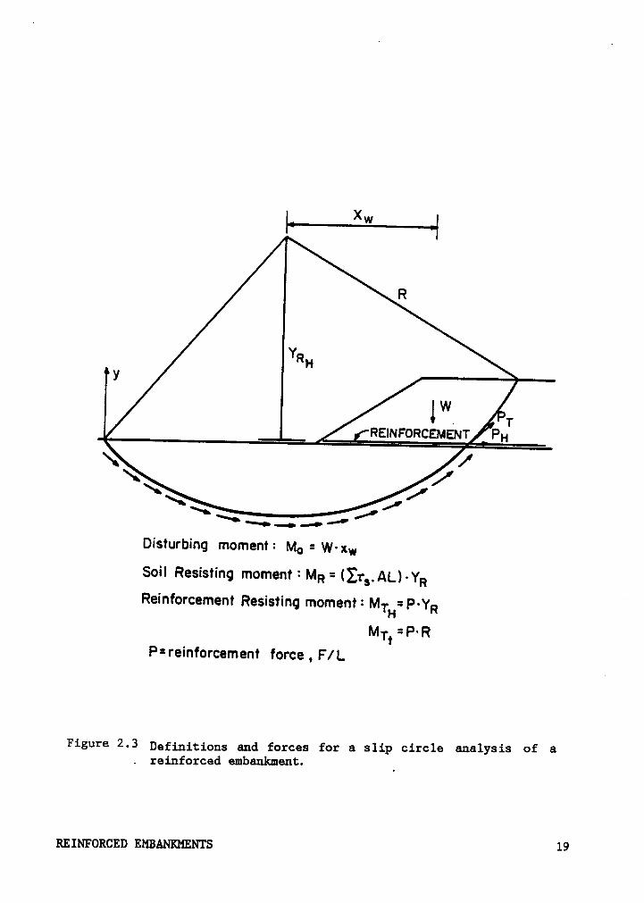
Figure 2.3 Definitions and forces for a slip circle analysis of a re-inforced embankment. .................. 19
Figure 2.4 Orientation of reinforcement at the slip surface. . . . 23
Figure 2-5 Approximate ratio of factor of safety calculated usingtangential and horizontal orientations (after Low, 1985). 26
Figure 2,6 Failure modes for reinforcement-soil interface in thefield. ......................... 28
Figure 2.7 Consideration of mobilized soil strength and reinforcement- forces under working conditions. ............ 30
Figure 2.8 Procedure for determining load-strain curves for creepsensitive reinforcing materials (McGown et al. 1984). . 32
Figure 2,9 Schematic representation of laboratory pullout and directshear tests. ...................... 35
Figure 2•]l)Determination of 1 for tests over a range of normalg stresses. ....................... 36
Figure 2.11.Variation of bond angle as determined in pullout tests(adapted from Ingold, 1982b). ............. 38
Figure 2.12 Interface strength of Tensar SR2 in pullout test (Rowe etal. 1985). ....................... 41
Figure 2.13 Strain compatibility of reinforcement and soil (McGown etal. 1984). ....................... 42
Figure 2-19 Allowable compatible strain as defined by Rowe andSoderman, 1985. .................... 45
Figureg_l5 Stability number versus percentage of reinforcement in co-
hesive soils (Brown and Poulos, 1978). ......... 52
Figure 2.16 Comparison between finite element and model tests results(Brown and Poulos, 1978). ............... 53
List of Illustrations xiv
Figure 2_l7 (a) Behavior of a stiff-stiff material system (b) Behaviorof a stiff-soft material system (after Jones and Edwards,1980) ......................... 54
Figure 2,18 Subsurface conditions at Pinto Pass. .......... 68
Figure 2.19 Construction sequence used at Pinto Pass. ....... 70
Figure 2,20 Test section geometry at Almere test site. ....... 73
Figure 2.21 Measured reinforcement forces at Almere (Brakel et al.1982). ......................... 75
Figure 2.22 Limit equilibrium results for Almere case history. . . . 76
Figure 2,23 Site conditions at Bloomington Road. .......... 78
Figure 2.24 Settlement at Station A. ................ 81
Figure 2-25 Settlement at Station B. ................82
Figure3_l Failure surfaces in CON2D86 (Duncan et al. 1981). . . . 90
Figure 3.2 The yield surface used in finite element analyses, in q-p'space. ......................... 91
Figure 3.3 Definition of Cam Clay parameters X and K. ....... 93
Figure 4,1 Reinforced foundations. ................ 102
Figure 4.2 Modes of failure identified by Binquet and Lee (1975). 105
Figure 4•3 Failure of soil below footing on dense sand layer abovesoft clay (Meyerhof 1974). ............... 111
Figure 4.4 Measured bearing capacities versus calculated values usingHanna and Meyerhof (1980) procedure. .......... 114
Figure 4-5 Comparison of measured and computed load-displacementcurves for UC Davis model tests - plane strain case. . . 121
Figure 4·6 Comparison of measured and computed load-displacementcurves for UC Davis model tests - axisymmetric case. . . 123
Figure 4,7 Mechanisms of deformation for reinforced sand over clay. 127
Figure 4.8 Zones around perimeter of three-dimensional footings wherereinforcement is less effective. ............ 133
List of Illustrations xv
Figure 4.9 Measured bearing capacities versus calculated values forthe reinforced case using Equation 4.6 or 4.7. ..... 134
Figure 5.1 Typical cross-section of Mohicanville Dike No. 2 showingfoundation conditions, old and new embankment limits, andundrained shear strengths (after Collins et al. 1982). 141
Figure 5.2 Distribution of required reinforcement force from stabil-ity analyses to provide a minimum factor of safety of 1.3(after Collins et al. 1982 and Fowler et al. 1983). . . 144
Figure 5.3 Reinforcement force and strength versus reinforcementstiffness (after Fowler et al. 1983). ......... 148
Figure 5.4 Stress-strain curves from consolidated undrained (CU)tests on the foundation clay (after Collins et al. 1982). 152
Figure 5_5 Stress-strain curves from unconsolidated undrained (UU)tests on the foundation clay (after Collins et al. 1982). 153
Figure 5,5 Compression curves from one—dimensional tests on thefoundation clay (Collins et al. 1982). ......... 154
Figure 5.7 Stress-strain curves from consolidated-undrained (CU)tests on the peat (Collins et al. 1982). ........ 156
Figure 5.8 Compression curves from one-dimensional tests on the peat(Collins et al. 1982). ................. 157
Figure 5.9 Variation of peat permeability with height of fill,adapted from Weber (1969) and Collins et al. (1982). . . 158
Figure 5.10 Stress-strain curves from consolidated-undrained (CU)tests on the old embankment fill (Collins et al. 1982). 159
Figure 5.11 Stress-strain curves from consolidated—undrained (CU)tests on the new embankment fill. ...... . .... 160
Figure $-12 Consolidation curve of embankment fill from an isotropiccompression test (Fowler et al. 1983). ......... 161
Figure 5-13 Plan view of the dike and location of the four instrumentedsections (adapted from Project Plans). ......... 164
Figure 5.14 Cross section at Station 4+75. ............. 167
Figure 5.15 Cross section at Station 6+55. ............. 168
Figure 5.16 Cross section at Station 9+00. ............. 169
List of Illustrations xvi
Figure 5-17 Cross section at Station 12+20. ............ 170
Figure 5·l8 Measured reinforcement forces at the centerline of theinstrumented sections. ................. 172
Figure 5.19 Measured reinforcement forces at the centerline of Station9+00. ......................... 175
Figure 5.20 Distribution of measured reinforcement forces about thecenterline at Station 6+55. .............. 176
Figure 5-21 Piezometric levels in the peat versus embankment height,measured at centerline stations. ............ 179
Figure 5.22 Piezometric levels in the foundation clay versusembankment height, measured at centerline stations. . . 180
Figure 5.23 Piezometric levels in foundation clay and peat atcenterline of Station 9+00. .............. 181
Figure 5-24 Piezometric levels in the foundation clay at Station 9+00. 182
Figure 5,25 Piezometric levels in the peat at Station 9+00. .... 183
Figure 5.26 Piezometric level in the peat at Station 6+55. ..... 184
Figure 5.27 Piezometric levels in the foundation clay at Station 6+55. 185
Figure 5_2g Measured settlement at Station 4+75. .......... 189
Figure 5,29 Measured settlement at Station 6+55. .......... 190
Figure 5.30 Measured settlement at Station 9+00. .......... 191
Figure 5_31 Measured settlement at Station 12+20. ......... 192
Figure 5,32 Measured horizontal movements at the toes at Station 6+55. 195
Figure 5.33 Measured horizontal movements upstream of centerline atStation 9+00. ..................... 196
Figure 5,34 Measured horizontal movements at Station 9+00. ..... 197
Figure 5.35 Comparison of calculated to measured stress-strain curvesfor foundation clay using initial parameters. ..... 202
Figure 5-36 Comparison of calculated and measured stress-strain curves‘
for foundation clay using adjusted M values. ...... 204
List of Illustrations xvii
Figure 5.37 Effect of changes in soil parameters on shape of stress-strain curves (after D'0razio and Duncan 1983). .... 205
Figure 5-38 Stress paths for samples from test series UD22. .... 208
Figure 5-39 Comparison of calculated to measured stress-strain curvesfor foundation clay for higher cell pressure sample. . . 209
Figure 5.40 Stress paths for samples from test series UD25. .... 210
Figure 5.41 Comparison of calculated to measured stress-strain curvesfor foundation clay for sample UD25. .......... 211
Figure 5-42 Stress paths followed in model used in analyses. .... 213
Figure 5,43 Comparison of calculated to measured stress-strain curvesfor foundation clay soil parameters used in analyses. 214
Figure 5.44 Comparison of calculated to measured stress-strain curvesfor peat soil parameters used in analyses. ....... 218
Figure 5·e5 Comparison of calculated to measured stress-strain curvesfor old fill soil parameters used in analyses. ..... 220
Figure 5_45 Final stress-strain curves used for new embankment fill. 221
Figure 5.47 Finte element mesh used for analysis of downstream partof Station 6+55. .................... 224
Figure 5-48 Finite element mesh used for analysis of upstream part ofStation 6+55. ..................... 225
Figure 5_49 Measured versus calculated reinforcement forces at thecenterline of Station 6+55. .............. 227
Figure 5.50 Measured versus calculated reinforcement forces distrib-uted about the centerline at Station 6+55. ....... 229
Figure 5•5l Measured versus calculated piezometric levels in the peat- Station 6+55. .................... 231
Figure 5.52 Measured versus calculated piezometric levels in thefoundation clay - Station 6+55. ............ 232
Figure 5-53 Measured versus calculated settlement - Station 6+55. 233
Figure 5·5‘·Measured versus calculated horizontal movements - Station6+55. ......................... 234
List of Illustrations xviii
Figure 5,55 Finite element mesh used for analysis of downstream partof Station 9+00. .................... 236
Figure 5,55 Measured versus calculated reinforcement forces at thecenterline - Station 9+00. ............... 237
Figure 5,57 Measured versus calculated piezometric levels - Station9+00. ......................... 239
Figure 5,58 Measured versus calculated settlement at Station 9+00. 240
Figure 5,59 Effects of ageing on strength of Vicksburg silty clay(after Trollope and Chan, 1960). ............ 243
Figure 5.60 Effects of ageing on strength and pore water pressure ofVicksburg silty clay and San Francisco Bay Mud (afterSeed, Mitchell and Chan, 1960). ............ 244
Figure 5.6l Grain size distribution of Mohicanville Dike No. 2embankment fill tested during this study. ....... 248
Figure 5.62 Moisture-density relations for clay tested. ...... 249
Figure 5.63 Stress-strain curves from UU tests on freshly compactedsoil. ......................... 252
Figure 5-64 Stress-strain curves from UU tests on samples aged oneweek. ......................... 253
Figure 5,55 Stress-strain curves from UU tests on samples aged twoweeks. ......................... 254
Figure 5,66 Stress-strain curves from UU tests on samples aged fourweeks. ......................... 255
Figure 5.67 Measured versus calculated reinforcement forces at thecenterline including effects of ageing on fill. .... 261
Figure 6.1. Soil profile at St. Alban site (after Pilot et al. 1982). 266
Figure 6.2. Typical consolidated undrained test results: stress-strain relationship and Poisson°s ratio (Tavenas et al.1974). ......................... 267
Figure 6.3. Consolidation characteristics for the soft clay (afterTavenas et al. 1974). ................. 269
Figure 6.4 (a) Typical dimensions of Tensar SR2. (b) Isochronousload-strain curves. (c) Typical tensile test results. 271
List of Illustrations xix
Figure 6,5 Undrained shear strength profiles of St. Alban site de-termined by different hypotheses (La Rochelle et al.1974). ......................... 277
Figure 6,6 Factors of safety versus geogrid strength for strip re-inforced embankment determined using STABGM. ...... 281
Figure 6,7 Template used for the finite element analyses. .... 284
Figure 6,8. Measured settlement behavior of the strip reinforcedembankment compared with calculated settlement usingCON2D86. ........................ 291
Figure 6,9 Measured horizontal movements at the toe of the stripreinforced embankment compared with calculated values us-ing CON2D86. ...................... 292
Figure 6,10 Measured geogrid forces in the strip reinforcedembankment compared with calculated reinforcement forcesusing CON2D86. ..................... 293
Figure 6,11 Measured piezometric levels in the foundation under thestrip reinforced embankment compared with calculated val-ues. .......................... 294
Figure 6,12 ueasured settlement behavior of the strip reinforcedembankment compared with calculated settlement usingSSTIPN. ........................ 298
Figure 6,13 Measured horizontal movements at the toe of the stripreinforced embankment compared with calculated values us-“ing SSTIPN. ...................... 299
Figure 6.14 Measured geogrid forces in the strip reinforcedembankment compared with calculated reinforcement forcesusing SSTIPN. ..................... 300
Figure 6,15 Measured settlement behavior of the geocell mattressembankment compared with calculated settlement usingSSTIPG. ........................ 303
Figure 6,16 Measured horizontal movements at the toe of the geocellmattress compared with calculated horizontal movementsusing SSTIPG. ..................... 304
Figure 6,17 Measured geogrid forces in the geocell mattress comparedwith calculated reinforcement forces using SSTIPG. . . . 305
Figure B-1 Axially symmetric membrane plate element: plan view,section view, and local coordinate system. ....... 358
List of Illustrations xx
Figure B-2. Relationship between equivalent modulus and the ratio of‘ the major and minor modulus values for bi-directionalgeogrids. ....................... 364
Figure C'l Nodal point numbering for two-dimensional elements. . . 368
Figure C·2. Nodal point numbering conventions for linkage elements. 370
Figure C—3 Linkage element example. ............... 371
Figure_C·4 Example mesh for an embankment dam. .......... 372
Figure C—$. Example meshes for embankment with pre-existing parts. 374
Figure C”6 Example data for construction layers. ......... 376
Figure C-7 Example data for distributed loads. .......... 377
Figure C‘8. Example data for changes in reservoir level. ..... 379
Figure D'l Nodal point numbering for two-dimensional elements. . . 397
Figure D-2p Nodal point numbering conventions for linkage elements. 399
Figure 0-3 Linkage element example. ............... 400
Figure F“4 Example mesh for tank foundation. ........... 40lF
Figure D—5 Example meshes with pre-existing parts. ........ 403
Figure D*6 Example data for construction layers. ......... 405
Figure D—7 Example data for distributed loads. .......... 407
Figure D·8 Example data for constant non-zero pore pressure. . . . 408
List of Illustrations xxi
List of Tables
Table 2.1 Limit equilibrium techniques applied to reinforcedembankments. ...................... 10
Table 2.2 Summary of bond angle determinations. .......... 39
Table 2.3 Finite element techniques applied to reinforced embankments. 49‘
Table 2.4 Comparison of ¢iand c' of peat from various tests (Rowe etal. 1984). ....................... 60
Table 2.5 Summary of Case History Performance Records. ...... 65
„ Table 4.1 Measured and calculated bearing capacities for generalshear. ......................... 130
Table 4.2 Measured and calculated bearing capacities for generalshear. ......................... 136
Table 5.1 Summary of soil properties. ............... 151
Table 5.2 Instrumentation at Mohicanville Dike No. 2. ....... 165
Table 5.3 Model parameters used in foundation clay trials. .... 201
Table 5.4 Consolidatad undrained tests on embankment clay. .... 219
Table 5.5 Summary of soil model parameters used in analyses. . . . 223
Table 5.6 Dry density (in pcf) and water content of UU specimens. 251
Table 5«7 Undrained shear strengths from UU tests ......... 257T
Table 5.8 Modulus determined by hyperbolic model. ......... 258
Table 5.9 Secant modulus at 800 psf shear strength. ........ 259
Table 6.1 Height to failure of test embankments. ......... 274
Table 6.2 Soil parameters used in CON2D86 analyses. ........ 286
Table 6,3 Soil parameters used in hyperbolic soil parameter analyses. 288
Table Aal Instrumentation at Mohicanville Dike No. 2. ....... 330
Table Ae2 Average crest elevations at instrumented sections. . . . 331
Table A—3 Ceuterline reinforcement forces (in tons/ft). ...... 332
List of Tables xxii
Table A-4 Reinforcement forces about centerline at Station 6+55. 333
Table A-5 Reinforcement forces about centerline at Station 9+00. 334
Table A-6 Piezometric locations and elevations. .......... 335
Table A-7 Piezometric elevations selected by station and date. . . 336
Table A—8 Settlement plate movements, settlement in feet. ..... 337
Table A-9 Elevations of surface displacemeut monuments by date. . . 338
Table A—l01nc1inometer information. ................ 339
Table A—llHorizontal movements at inclinometer 1-1 in feet. .... 340
Table A—l2Hbrizontal movements at inclinometer 1-5 in feet. .... 341
Table A—l3Horizontal movements at inclinometer 1-6 in feet. .... 342
Table A-l4Horizonta1 movements at inclinometer 1-7 in feet. .... 343
Table A—l5Horizonta1 movements at inclinometer 1-8 in feet. .... 344
Table A-l6Horizonta1 movements at inclinometer 1-9 in feet. .... 345
Table A-l7Vertical settlements at inclinometer 1-10 in feet. . . . 346
Table A—l8Vertical settlements at inclincmeter 1-11 in feet. . . . 347
Table A-l9Vertica1 settlements at inclinometer 1-12 in feet. . . . 348
Table A-2OVertica1 settlements at inclinometer I-13 in feet. . . . 349
Table A-2lHorizonta1 movements at inclinometer 1-14 in feet. . . . 350
Table A—22Hbrizontal movements at inclinometer 1-15 in feet. . . . 351
List of Tables xxiii
CHAPTER I
INTRODUCTION
Soil is one of the cheapest and most effective construction materials.
When compacted, it finds use as subgrades for our roads, abutments for
our bridges, foundations for structures, and fills for embankments and
retaining walls, to name just a few. Despite its wide application, soil
has inherent shortcomings in its structural capabilities; namely, it is
unable to sustain tension or high levels of shear. This limits its use
in certain applications. Within the last 20 years, however, it has been
shown that soil can be reinforced with systems of small structural ele-
ments, thereby providing the needed tensile and shear strength and
stiffness. With the advent of this new technology, many new applications
have been developed including reinforced soil retaining walls,
embankments and foundations.
The concept of strengthening soil by the addition of reinforcing ma-
„ terials is very old. Indeed, the basic principles are demonstrated in
nature by birds and animals in the construction of nests and lodges. The
reinforcement of clay bricks using reeds or straw probably began very
early in civilization. Jones (1985) provides a detailed account of the
historical record of the use of reinforced soil. .
One of the examples Jones cites is that of a ziggurrat of the ancient
city of Dur·Kurigatzu, now known as Agar—Quf. The ziggurrat, which is
an ancient temple tower, is located five kilometers north of Baghdad.
INTRODUCTION 1

It was constructed of clay bricks varying in thickness between 130-400
mm, reinforced with woven mats of reed laid horizontally on a layer of
sand and gravel at vertical spacings between 0.5 and 2.0 m. This struc-
ture is presently 45 m tall, although it is estimated that its original
height was around 80 m. It is thought to be over 3000 years old.
Other examples include reed-reinforced earth levees built by the
Romans along the Tiber River; the Great Wall of China containing mixtures
of clay and gravel reinforced with tamarisk branches; fortifications of
alternate layers of logs and earth fill constructed by the Gauls; and the
construction of earth retaining walls in the U.S. using wooden re-
inforcement by Munster as early as 1925.
The modern concept of reinforcing soil to resist tensile forces by
the use of an indigenous material was proposed in the 1930's by Arthur
Casagrande who idealized the problem in the form of a weak soil reinforced
by high-strength membranes laid in horizontal layers. Holtz (1977) re-
ports that Casagrande envisioned the use of steel rods and plates to re-
inforce embankments on weak soils, but rejected their use as uneconomical.
Westergaard (1938) proposed an analytical approach to the problem in a
paper in the 60th Anniversary Volume on Solid Mechanics dedicated to
Stephen Timoshenko.
It was not until the work of a Frenchman, Henri Vidal, in the 1960's,
however, that the use of reinforcement in soils became a practical matter.
Vidal developed a system of earth reinforcement using horizontal metal
strips behind a facing to construct vertical reinforced earth walls. The
design procedures espoused by Vidal (1969) are based on the development
INTRODUCTION 2
of adhesion or interaction between the reinforcement and the soil due to
friction of sufficient means to restrain the soil as if acted upon by a
lateral force equivalent to the at-rest pressure.
Since Vidal's pioneering work many different reinforcing materials
have been developed, notably in the area of polymer-based materials.
Today the use of steel bars, wire meshes, high-density polyethylene grids,
woven and non-woven textiles, root mats and various forms of wood as re-
inforcement are commonplace in the construction of retaining walls,
bridge abutments, dams, highway embankments, landslide repair and road
construction over soft soils.
Although the use of reinforcement in soils has been one of the leading
new technologies in the area of geotechnical engineering, the development
of rational design methods has not always kept pace with the new appli-
cations of reinforced soil or the new materials proposed for use as re-
inforcement. Since the l960°s, a wealth of literature on soil
reinforcement has developed, much of it pertaining to the use of rein-
forced soil in retaining structures. It is only recently that attention
has turned to the application of reinforced soil embankments and founda-
tions overlying soft soils.
In this light, this study was directed to development of a rational
understanding of the analysis and design of reinforced soil structures
overlying weak or soft soils. To this end there are two numerical ap-
proaches which, may be applied rationally - namely limit equilibrium
methods and finite element methods. Both of these approaches have found
considerable use in geotechnical engineering, yet advances and confidence
INTRODUCTION 3

in their use has come only when the numerical results have been tested
against actual behavior of geotechnical structures. Therefore, the
analysis of well-documented case histories formed a significant part of
the work performed in this study.
Chapter II reviews the literature on reinforced embankments and de-
scribes many of the factors which come into play when analyzing reinforced
embankments. In this study, a finite element code was adapted for the
analysis of reinforced soil structures over soft soils, and this is de-
scribed in Chapter III. In Chapter IV, a brief review of reinforced
foundations is presented and a method for determining the bearing capacity
of reinforced foundations over soft clay is proposed and compared to
available model test data. The applicability of the finite element method
for analysis of reinforced foundations is also considered in Chapter IV.
In Chapters V and VI, the finite element method is used to analyze case
histories, and the calculated and measured behavior of reinforced
embankments on weak soils are compared. A summary is presented in Chapter
VII.
INTRODUCTION 4
CHAPTER II
REINFORCED EMBANKMENTS
2.1 Introduction
Using reinforced soils in embankments is a relatively recent practice,
springing from the need to construct haul roads and earth dams on rela-
tively weak soils and road embankments in areas short on right·of-way.
Reinforcement of soil allows construction of slopes and embankments hav-
ing steep side slopes and over weak foundation soils. Early design pro-
cedures for embankments over good foundation subsoils followed the
successful procedures used in the design of reinforced soil retaining
walls (Jewell et al. 1984 and Leshchinsky 1984). It was a relatively
straightforward matter to extend procedures for vertical retaining walls
to those sloping from 30° to 80° from the horizontal. The analysis of
reinforced embankments over weak subsoils is somewhat more complex owing
to uncertainties introduced by the weak subsoils.
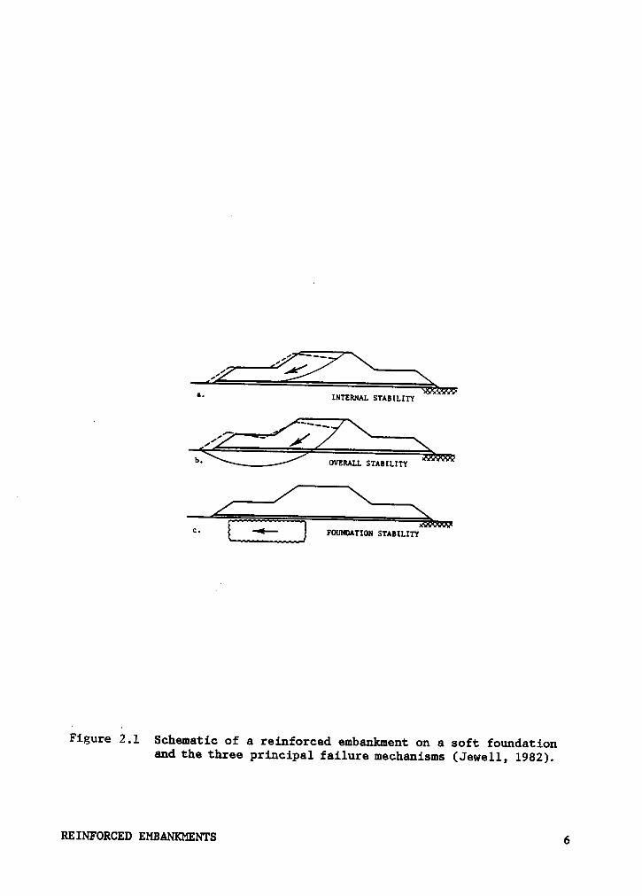
The successful design of a reinforced embankment must take account
of the internal stability of the embankment, the overall stability of the
embankment and foundation, and the stability of the foundation. These
conditions are illustrated in Figure 2.1.
Internal stability can be evaluated by computing the resistance to
sliding of the embankment over the reinforcement. This is accomplished
by calculating the horizontal force exerted by the embankment and the
REINFORCED EMBANKMENTS 5
*· INTERNALSTABILITYb.
OVBRALL STABILITYY,-nrw
C- FGUNDATION STABILITY
Figure 2.1 Schematic of a reinforced embankment on a soft foundationand the three principal failure mechanisms (Jewell, 1982).
REINFORCED EMBANKMENTS 6
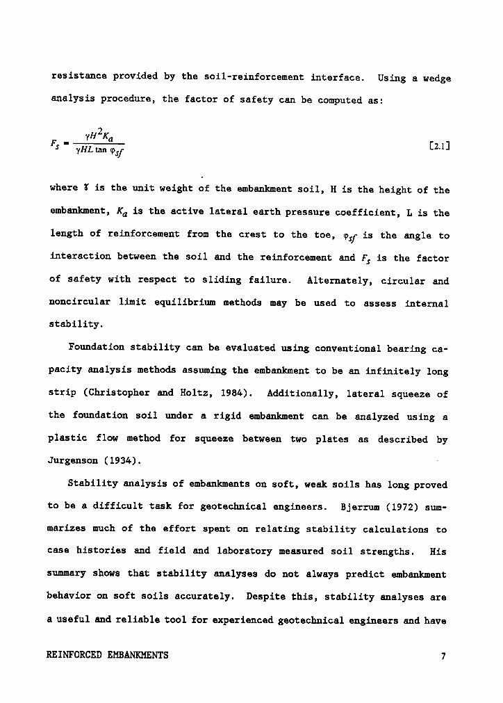
resistance provided by the soil-reinforcement interface. Using a wedge
analysis procedure, the factor of safety can be computed as:
2rs = [2.1]
where K is the unit weight of the embankment soil, H is the height of the
embankment, Kb is the active leteral earth pressure coefficient, L is the
length of reinforcement from the crest to the toe, eg-is the angle to
interaction between the soil and the reinforcement and F} is the factor
of safety with respect to sliding failure. Alternately, circular and
noncircular limit equilibrium methods may be used to assess internal
stability.
Foundation stability can be evaluated using conventional bearing ca-
pacity analysis methods assuming the embankment to be an infinitely long
strip (Christopher and Holtz, 1984). Additionally, lateral squeeze of
the foundation soil under a rigid embankment can be analyzed using a
plastic flow method for squeeze between two plates as described by‘
Jurgenson (1934). ‘
Stability analysis of embankments on soft, week soils has long proved
to be a difficult task for geotechnical engineers. Bjerrum (1972) sum-
marizes much of the effort spent on relating stability calculations to
case histories and field and laboretory measured soil strengths. His
summary shows that stability analyses do not always predict embankment
behavior on soft soils accurately. Despite this, stability anelyses are
a useful and reliable tool for experienced geotechnical engineers and have
REINFORCED EMBANKMENTS 7
remained the dominant analysis procedure. In addition, finite element
techniques have been used to gain further insight into embankment behavior
(Duncan, 1972).
The procedures used for analysis and design of reinforced embankments
have naturally followed those used for unreinforced embankments. Thus
limit equilibrium and finite element analyses have been used to analyze
and design reinforced embankments. The application of these procedures
to reinforced embankments is more fully described below.
2.2 Limit Equilibrium Methods
2.2.1 General
The use of limit equilibrium techniques for analyzing unreinforced
slopes and embankments is well accepted geotechnical engineering prac-
tice. The extension of these procedures to reinforced slopes and
embankments is, however, not always straightforward. Uncertainties exist
in the procedure used to incorporate the reinforcement strength into the
stability analysis, the strength of the reinforcement to input into the
analysis, the mechanism of soil-reinforcement interaction, all this in
addition to the usual uncertainties in regard to construction on soft
soils. An analysis of the stabi1ity· of a reinforced soil slope or
embankment requires consideration of both the external forces necessary
to maintain stability and the internal forces necessary to ensure re-
inforcement integrity.
REINFORCED EMBANKMENTS 8
Several limit equilibrium approaches have been proposed for the
analysis of reinforced embankments. While most of these methods involve
some type of modification of common slip circle analysis, there are dis-
tinct differences in the details of the modifications proposed. Common
to all of the methods is the assumption of rigid-plastic soil behavior.
Additionally, most of these methods make no provision for embankment-
reinforcement interaction and deformation behavior.
The details of several limit equilibrium techniques are summarized
in Table 2.1. As may be seen, the approaches include extension of the
Ordinary Method of Slices, extension of Bishop°s Modified Method, the use
wedge-type analyses, and the use of variational calculus combined with
extremization.
The first extension of limit equilibrium methods to the design of
reinforced embankments appears to be that of Wager (1968) who analyzed
an anchored sheetpile wall used to reinforce a road embankment on a soft
subsoil. The analysis consisted of adding a resisting moment due to the
anchor force to the resisting moment along a circular slip surface in the
foundation. The method was presented in English by Wager and Holtz
(1976). Broms (1977) discussed Wager°s procedure and how it could be
applied to polyester fabric reinforced embankments. Christopher and
Holtz (1984) report that the procedure has been successfully applied in
30 or so cases.
Christie and El-Hadi (1977) proposed an extension to the Ordinary
Method of Slices (OMS) to account for horizontal forces necessary to
maintain stability. In their formulation, the factor of safety applied
REINFORCED EMBANKMENTS 9
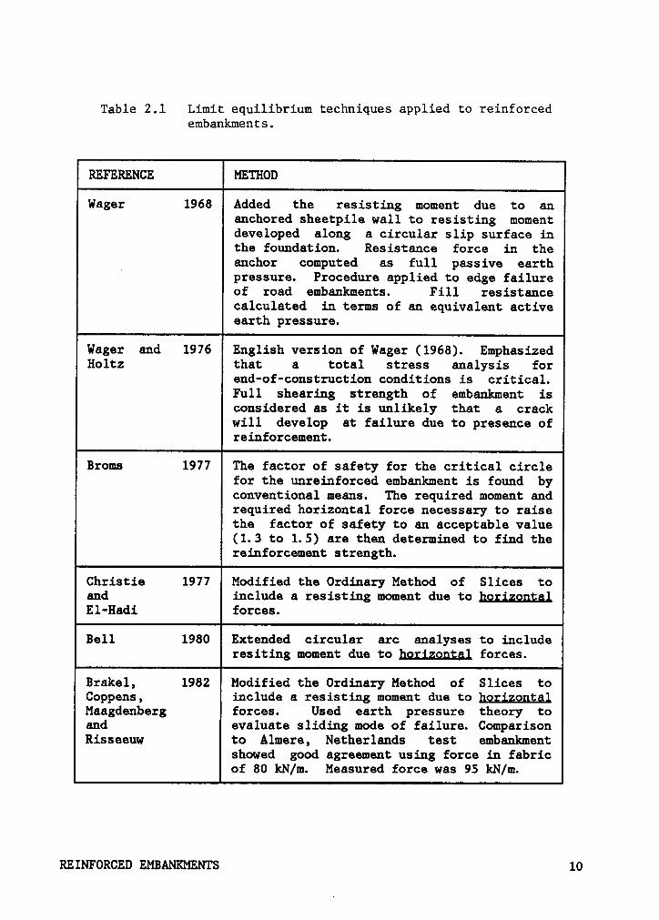
Table 2.1 Limit equilibrium techniques applied to reinforcedembankments.
Wager 1968 Added the resisting moment due to ananchored sheetpile wall to resisting momentdeveloped along a circular slip surface inthe foundation. Resistance force in the
_ anchor computed as full passive earthpressure. Procedure applied to edge failureof road embankments. Fill resistancecalculated in terms of an equivalent activeearth pressure.
Wager and 1976 English version of Wager (1968). EmphasizedHoltz that a total stress analysis for
end-of-construction conditions is critical.Full shearing· strength of embankment isconsidered as it is unlikely that a crackwill develop at failure due to presence ofreinforcement.
Broms 1977 The factor of safety for the critical circlefor the unreinforced embankment is found byconventional means. The required moment andrequired horizontal force necessary to raisethe factor of safety to an acceptable value(1.3 to 1.5) are then determined to find thereinforcement strength.
Christie 1977 Modified the Ordinary Method of Slices toand include a resisting moment due to hggjzggtglEl—Hadi forces.
Bell 1980 Extended circular arc analyses to includeresiting moment due to hggizggtgl forces.
Brakel, 1982 Modified the Ordinary Method of Slices toCoppens, include a resisting moment due to hgrigggtalMaagdenberg forces. Used earth pressure theory toand evaluate sliding mode of failure. ComparisonRisseeuw to Almere, Netherlands test embankment
showed good agreement using force in fabricof 80 kN/m. Measured force was 95 kN/m.
REINFORCED EMBANKMENTS 10
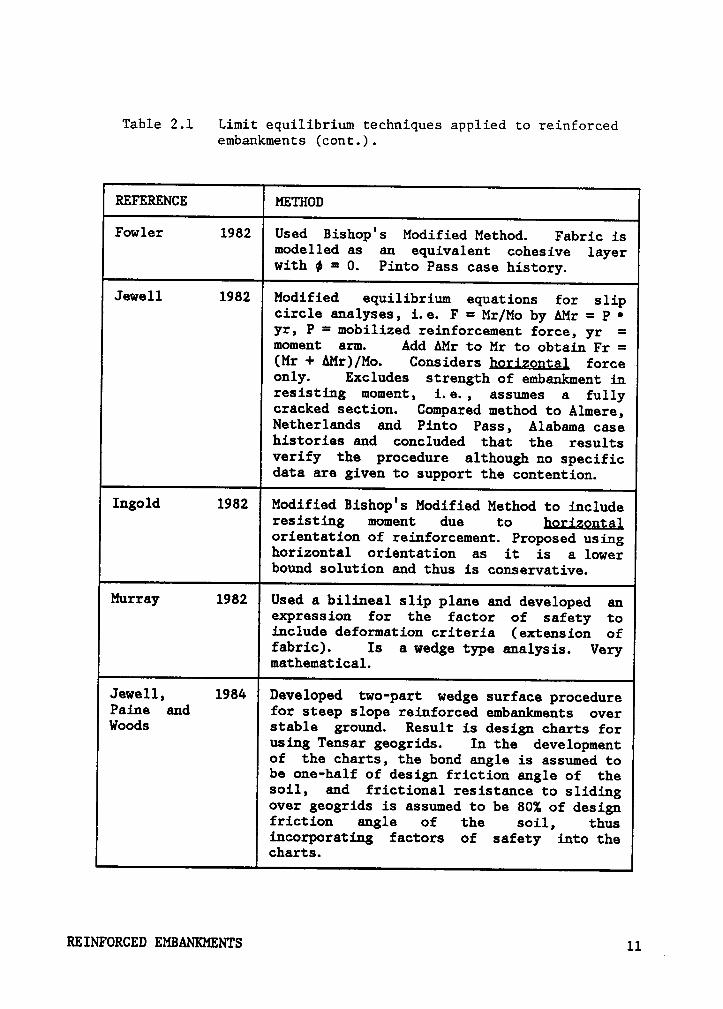
Table 2.1 Limit equilibrium techniques applied to reinforcedembankments (cont.).
DMODFowler 1982 Used Bishop°s Modified Method. Fabric is
modelled as an equivalent cohesive layerwith ¢ = 0. Pinto Pass case history.
Jewell 1982 Modified equilibrium equations for slipcircle analyses, i.e. F = Mr/Mo by AMr = P
•yr, P = mobilized reinforcement force, yr =moment arm. Add AMr to Mr to obtain Fr =(Mr + AMr)/Mo. Considers hggizggtal forceonly. Excludes strength of embankment inresisting moment, i.e., assumes a fullycracked section. Compared method to Almere,Netherlands and Pinto Pass, Alabama casehistories and concluded that the resultsverify the procedure although no specificdata are given to support the contention.
Ingold 1982 Modified Bishop°s Modified Method to includeresisting moment due to hggjgggtglorientation of reinforcement. Proposed usinghorizontal orientation as it is a lowerbound solution and thus is conservative.
Murray 1982 Used a bilineal slip plane and developed anexpression for the factor of safety toinclude deformation criteria (extension offabric). Is a wedge type analysis. Verymathematical.
Jewell, 1984 Developed two·part wedge surface procedurePaine and for steep slope reinforced embankments overWoods stable ground. Result is design charts for
using Tensar geogrids. In the developmentof the charts, the bond angle is assumed tobe one-half of design friction angle of thesoil, and frictional resistance to slidingover geogrids is assumed to be 80% of designfriction angle of the soil, thusincorporating factors of safety into thecharts.
REINFORCED EMBANKMENTS 11
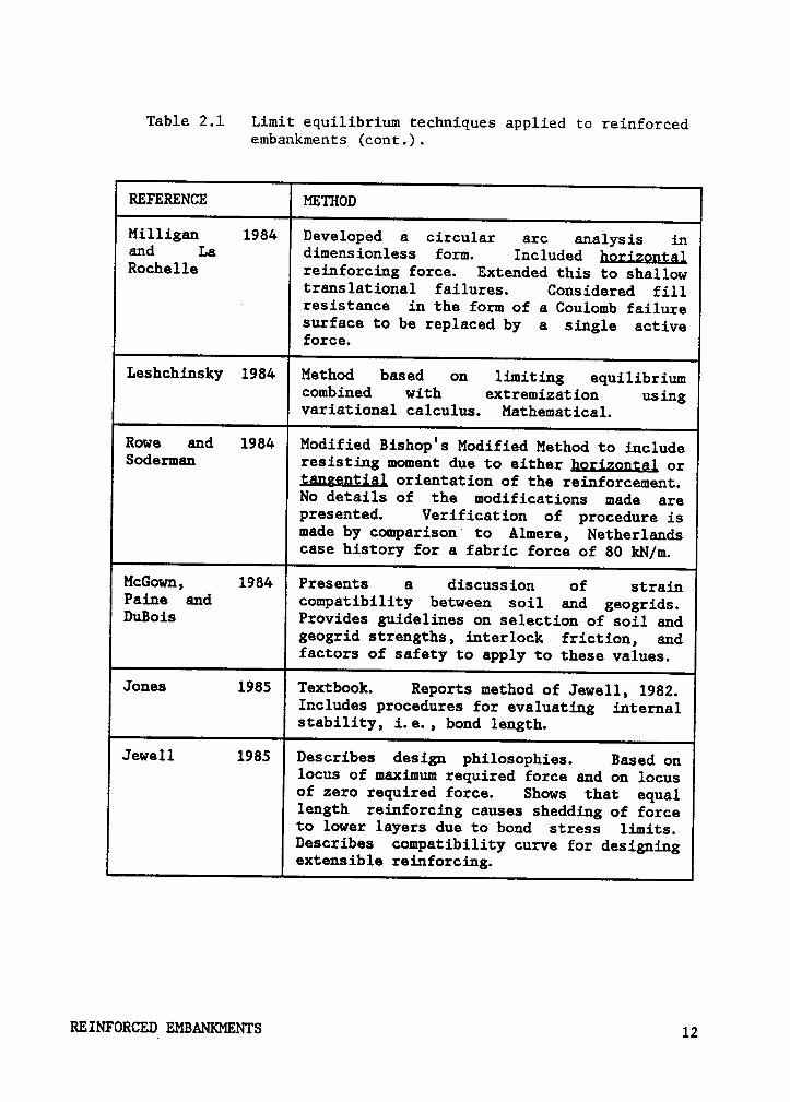
Table 2.l Limit equilibrium techniques applied to reinforcedembankments (cont.).
Milligan 1984 Developed a circular arc analysis inand La dimensionless form. Included hggjgggtglRochelle reinforcing force. Extended this to shallow
translational failures. Considered fill· resistance in the form of a Coulomb failure
surface to be replaced by a single activeforce.
Leshchinsky 1984 Method based on limiting equilibriumcombined with extremization usingvariational calculus. Mathematical.
Rowe and 1984 Modified Bishop°s Modified Method to includeSoderman resisting moment due to either hggizggtgl or
tgggggjgl orientation of the reinforcement.No details of the modifications made arepresented. Verification of procedure ismade by comparison‘ to Almere, Netherlandscase history for a fabric force of 80 kN/m.
McGown, 1984 Presents a discussion of strainPaine and compatibility between soil and geogrids.DuBois Provides guidelines on selection of soil and
geogrid strengths, interlock friction, andfactors of safety to apply to these values.
Jones 1985 Textbook. Reports method of Jewell, 1982.Includes procedures for evaluating internalstability, i.e., bond length.
Jewell 1985 Describes design philosophies. Based onlocus of maximum required force and on locusof zero required force. Shows that equallength reinforcing causes shedding of forceto lower layers due to bond stress limits.Describes compatibility curve for designingextensible reinforcing.
REINFORCED EMBANKMENTS 12
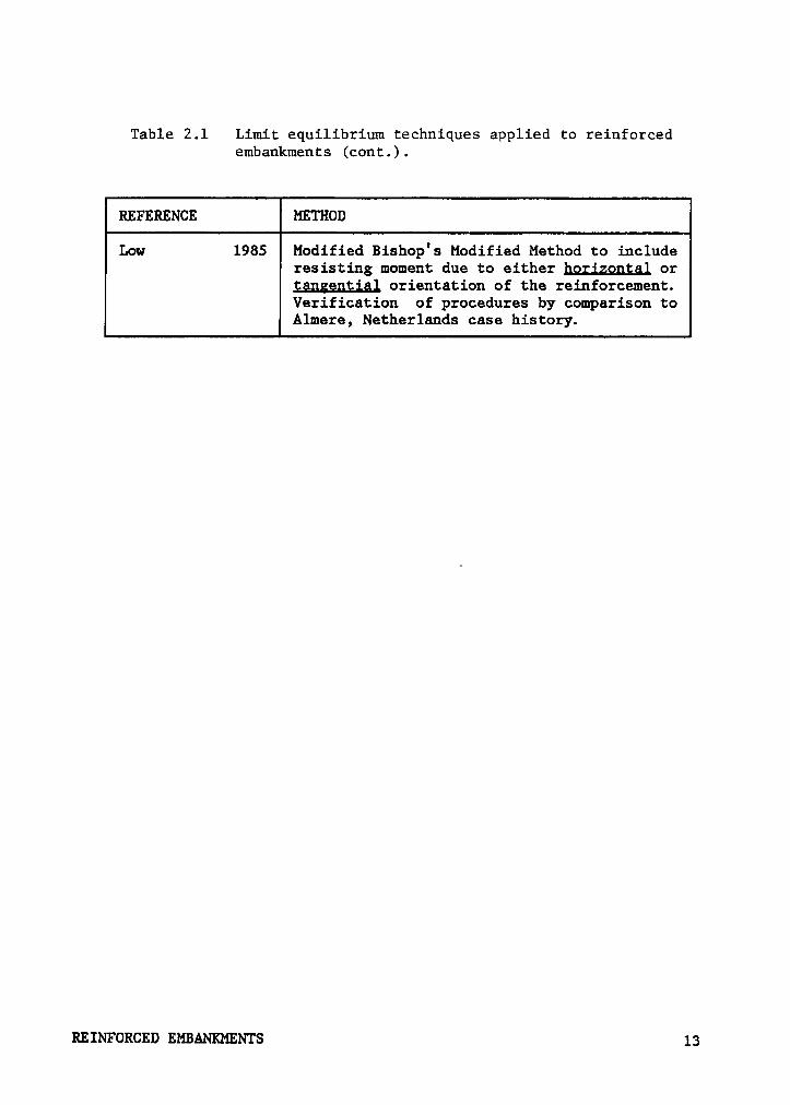
Table 2.1 Limit equilibrium techniques applied to reinforcedembankments (cont.).
REFERENCE METHOD
Low 1985 Modified Bishop's Modified Method to includeresisting moment due to either hggizggtal orggggggtigl orientation of the reinforcement.Verification of procedures by comparison to
„ Almere, Netherlands case history.
REINFORCED EMBANKMENTS 13

to the soil strength is also applied to the reinforcement force. Bell
(1980) also proposed extending circular arc analyses for horizontal re-
inforcement forces. Brakel et al. (1982) proposed adding a counteracting
moment due to the reinforcement force acting tangential to the slip sur-
face to the unreinforced OMS slip circle analysis.
Wedge type analyses have been developed by Murray (1982) and Jewell,
Paine and Woods (1984). Murray (1982) used a bilineal slip plane and
incorporated deformation criteria for the reinforcement in the analysis
to arrive at expressions for the factor of safety. Jewell, Paine and
Woods used two part wedge analysis to consider the slip surface develop-
ment in reinforced embankments over stable foundations.
A procedure based on limiting equilibrium combined with extremization
using variational calculus was developed by Leshchinsky (1984). Charts
have been developed from this procedure and are applicable to reinforced
embankments on stable foundations with slope angles varying from 30° to
90° (Leshchinsky and Volk, 1984).
Bishop°s Modified Method (BMM) has been used extensively in the
analysis of unreinforced embankments and has subsequently been used in
the analysis of reinforced embankments. Fowler (1982) modelled the re-
inforcement as an equivalent cohesive layer with o = 0 in a BMM analysis.
Ingold (1982a) extended Bishop's Modified Method to account for horizon-
tal orientation of reinforcement, but recognized that the assumption of
horizontal orientation was conservative. Rowe and Soderman (1984) and
Low (1985) have extended Bishop°s Modified Method to include either hor-
REINFORCED EMBANKMENTS 14
izontal or tangential orientation of the reinforcement at the failure
surface.
In these extensions, a restoring moment due to the fabric force is
added to the unreinforced restoring moment, assuming the reinforcement
force acts either parallel to the original reinforcement position (i.e.,
horizontal) or tangential to the slip surface at the point of intersection
of the slip circle surface and the reinforcement. The subject of orien-
tation of the reinforcement force at failure is discussed in more detail
in Section 2.2.3. Low showed that the manner in which the factor of
safety is defined is important. The effect of the reinforcement can be
included in the definition of factor of safety in two ways: as an addi-
tional force resisting failure or as a reduction in the forces causing
failure. This concept is explored in more detail below.
More recently Rowe and Soderman (1985) have extended their method tol
include a more rigorous treatment of the compatibility between soil
strains and reinforcement strains. This is discussed in more detail in
Section 2.2.4.
Milligan and La Rochelle (1984) have correctly pointed out that ex-
tending conventional limit equilibrium procedures to include the effects
of reinforcement does not eliminate the errors and uncertainties which
exist in current unreinforced stability analyses.
Chart solutions for simple configurations of embankment and foundation
geometries and various reinforcement strengths have been prepared by
Fowler (1982), Ingold (1982a), Rowe (1984), Leshchinsky and Volk (1984)
and Low (1985).
REINFORCED EMBANKMENTS 15
2.2.2 Definition of Factor of Safety
The factor of safety without reinforcement may be defined as the
factor by which the shear strength must be divided to bring the slope into
a state of barely stable equilibrium:
_ shear strengthFo —shear stress required for equilibrium [22]
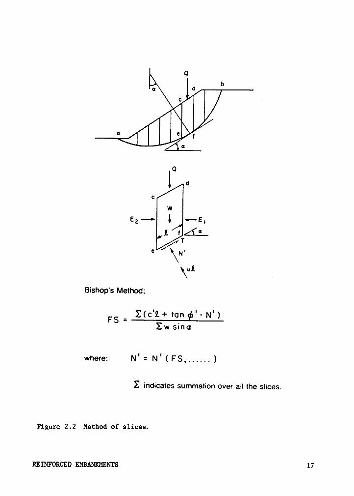
To evaluate the shear stress required for equilibrium, the geometry of
of the problem is divided into a number of slices as shown in Figure 2.2
and moments are summed about the center of the circular arc. By satis-
fying the equations of equilibrium, both the shear strength and the shear
stress can be expressed in terms of the geometry of the slope and the
properties of the soil. The resulting factor of safety may be expressed
in terms of moments as:
M12Fo - E [2.3]
where A(R is the resisting moment of the soil and AQ, is the overturning
moment. Formulation of the Ordinary Method of Slices (OMS) and Bishop°s
Modified Method (BMM) are obtained by summing appropriate moments and are
described in many soil mechanics textbooks, for example, see Lambe and
Whitman (1979).
The factor of safety of a reinforced slope or embankment my be ex-
pressed as:
REINFORCED EMBANKMENTS 16
O
¤q d
° rG
O
1 dc
EZ*’ •*'
E
G/’ Te \N•\ul
Bishop°s Method;
Z(c°2.+ ton f' - N°)FS = .E w sm a
where: N°=N‘(FS,...... )
X indicates summation over all the slices.
Figure 2.2 Method of slices.
RE1NFORcE¤ EMBAN1<MEN1*s 17

FR = [2.4]
where MT is the resisting moment of the reinforcement, and MR and Mo
are as previously defined. These definitions, as applied to a slip cir-
cle, are shown in Figure 2.3. An implicit assumption in this definition
is that there are no interactions between the soil and reinforcement that
change the individual contributions of A{R and Aßr.
Equation 2.4 can be rearranged in the following form:
MO [2.5]
from which it is evident that the definition of ER as given by Equation
2.4 implies that both the soil resisting moment and the reinforcement
resisting moment are divided by the same factor FR to bring the slopel
or embankment to a condition of barely stable equilibrium.
It should be emphasized that the term bfr in Eqns. 2.4 and 2.5 re-
presents the potential resisting moment that the reinforcement is capable
of providing, given sufficient strain. The enhanced safety of a rein-
forced embankment may not be noticeable at working conditions if the
mobilized force in the reinforcement is small. Nevertheless, the poten-
tial strength of the reinforcement is latent in the system and provides
an added margin of safety. A reinforced embankment not close to failure
might exhibit almost the same behavior as its unreinforced counterpart.
However, if both embankment heights were increased gradually (or, equiv-
alently, if foundation shear strength was decreased gradually), the re-
REINFORCED EMBANKMENTS 18
I XwI
R
Y
lw ·. 1-REINFORCEMENT PH
\ /'*‘€—• --9 ""
Disturbing moment= Mo = W·x,„
Soil Resisting moment = MR = (X·z·s.A|.) ·YRReinforcement Resisting moment= M1-H= P·YR
F
MT, = P' RP=reinfo¤-cement force , F/L
Figure 2•3 Definitions and forces for a slip circle analysis of a. reinforced embankment. _
REINFORCED EMBANKMENTS 19
inforced embankment would eventually reach a greater height (or withstand
a smaller foundation shear strength) than the unreinforced embankment
before a failure would occur.
The definition of FR may also be considered in terms of the rein-
forcing moment playing the role of reducing the overturning moment. In
this case the force is an external one and the factor of safety, with
stabilizing force T, is defined as:
MPR = [2.6]
where AVT is the moment due to the force T. Equation 2.6 can be rear-l
ranged as follows:
Mo = + MT [2.7]
It is thus clear that in this case the externally applied reinforcing
moment M'T is not divided byF’R
in formulating the equilibrium condition.
A factor of safety can be applied to the soil resisting moment and
the reinforcing resisting moment, thus obtaining a the factor of safety
for the system. This is not the case in Equation 2.6 and thus the pre-
ceding discussions make it clear that the factor of safety as defined by
Equation 2.4 is the more appropriate one for a reinforced embankment or
slope.
The improvement in the factor of safety due to reinforcement may be
incorporated in a stability analysis by adding to the factor of
REINFORCED EMBANKMENTS 20
safety for the same circle without reinforcement as calculated by the OMS
or BMM, and results in
FR = Fo + Ü [2.8]Mb
where Fb is the unreinforced factor of safety calculated by Eqn. 2.2 or
2.3. The value of ÄÖT is dependent upon the reinforcement orientation,
which can be specified to be either horizontal or tangential to the slip
surface, as discussed in the next section. ALT may then defined within a
computer program as:
MT;} Yc)] [2.90]
or
MT} = E[TgRadius of slip circlc)] [2.9b]
where
ALTR.: resisting moment due to reinforcement with horizontal orientation.ALT},= resisting moment due to reinforcement with tangential orientation.T}:. force in i-th layer of reinforcement where it is intersected by the
slip circle.Y}: Y coordinate of reinforcement.M.: Y coordinate of circle center.
The force in a layer of reinforcement can be varied along the length of
the reinforcement.
Two assumptions are inherent in the definition of the factor of
safety:
REINFORCED EMBANKMENTS 21
1. The potential slip surface intersects the reinforcement far from the
free end of the reinforcement so that if failure occurs, the full
strength of the reinforcement can be developed. This is a requirement
of sufficient anchorage to develop the full strength. of the re-
inforcement.
2. The will be no relative slip between the reinforcement and the soil.
Thus, in practical application of the methods discussed above, a separate
determination of the proper reinforcement force to use must be made, as
well as checking that soil-reinforcement bond is sufficient. These con-
cepts are explored in further detail in Sections 2.2.4 and 2.2.5, re-
spectively.
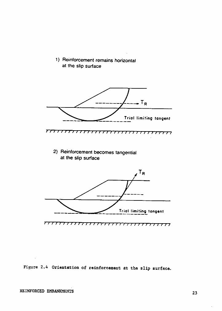
2.2.3 Orientation of Reinforcement at the Slip Surface
The possibility of the reinforcement orientation being changed due
to the relative movement of soil along the slip surface has been consid-
ered by Romstad et al. (1978), Rowe and Soderman (1984) and Leshchinsky
(1984), Low (1985) and others. There are two directions commonly assumed.
The first is that the reinforcement force acts horizontally as shown in
Figure 2.4a. The second assumes a tangential orientation to the slip
surface as depicted in Figure 2.4b. The need to consider reinforcement
orientation arises because relative movement along the slip surface may
change the orientation.
REINFORCED EMBANKMENTS 22
1) Fleinforcement remains horizontalat the slip surface
Trial limitinq tanqenl
2) Reinforcement becomes tangentialat the slip surface
TR
Trial limiting tanqent
Figure 2.4 Orientation of reinforcement at the slip surface.
REINFORCED EMBANKMENTS 23

At working conditions with a factor of safety greater than unity the
relative displacement of the soil along the slip surface may be too small
to change the orientation of the reinforcement significantly. Neverthe—
less, since ER is defined in terms of the potential strength of the re-
inforcement, it seems consistent with this notion to use potential
orientation (the orientation that the reinforcement is likely to assume
at failure) in combination with the potential strength of the reinforce-
ment when computing the potential reinforcing moment, IWT for use in
Equation 2.4.
The orientation at failure of an initially horizontal reinforcement
naturally depends on the flexural rigidity of the reinforcement. The two
diagrams in Figure 2.4 represent the extreme possible orientations of
initially horizontal reinforcement at failure. The situation shown in
the top diagram would be realistic in the extreme case of very stiff steel
bar reinforcement whereas that shown in the bottom diagram is only pos-
sible in the case of reinforcement having negligible flexural rigidity.
It should be noted that when the reinforcement is tangentially ori-
ented at the slip surface, it probably has less effect on the normal force
acting on the slip surface than when the reinforcement remains horizontal.
For the condition shown in Figure 2.4, the normal force and consequently
the shear strength of the soil near the slip surface would be increased
as a result of the normal component of the reinforcing force. This effect
is ignored in conventional limit equilibrium analyses. In contrast, the
orientation in the bottom diagram leads to a longer lever arm and hence
greater potential resisting moment from the reinforcement, although the
REINFORCED EMBANKMENTS 24

normal force on the slip surface and the increase in the strength of the
soil would likely be smaller in this case. There thus may be some com-
pensating effects that would tend to keep the overall resistance about
the same as the orientation of the reinforcement changes. The factor of
safety calculated assuming tangentially oriented and horizontally ori-
ented reinforcement are believed to represent reasonable values of the
upper and lower bounds for the reinforced factor of safety.
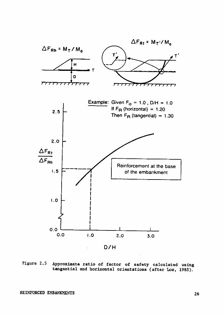
A computer program based on Bishop's Modified Method and the defi-
nition of AMT described above has been developed and is capable of com-
puting the factor of safety assuming either horizontally oriented
reinforcement or tangentially oriented reinforcement, (Duncan et al.
1985). The approximate relationship between the ratio of i%%ä~and {T
was developed by Low (1985) and is shown in Figure 2.5. In this figure,
ER, is the increase in the factor of safety with tangential oriented re-
inforcement, and FRh is that corresponding to horizontal oriented re-
inforcement. It can be seen that the factor of safety due to tangential
oriented reinforcement is always larger than that due to horizontal ori-
ented reinforcement and that the ratio of the two increases as the depth
of the weak foundation increases. The work by Low (1985) and Rowe and
Soderman (1984, 1985) suggests that using the average of the factor of
safety obtained from trials considering horizontal and tangential orien-
tations yields satisfactory and conservative design results.
REINFORCED EMBANKMENTS 25
APR} = MT'/ MuAPM = M 1- / M.,
TI
HT
D
Example: Given Fo = 1.0, 0/H = 1.0
2 5 If FR (horizontal) = 1.20' Then FR (tangential) = 1.30
2.0
AFmAPM .Fieinforcement at the base1.5 I of the embankment
III
I1.0IIIIII
o.o —-—I—-0.0 1.0 2.0 3.0
» D/ H
Figure 2.5 Approximate ratio of factor of safety calculated usingtangential and horizontal orientations (after Low, 1985).
REINFORCED EMBANKMENTS 26

2.2.4 Selection of Reinforcement Forces for Design
The use of limit equilibrium procedures results in a factor of safety
with respect to the ultimate limit state and is based on the potentially
realizable strengths of both the soil and the reinforcement. For soil
this strength is normally its peak value, however, for strain softening
soils this may be its residual strength. The strength of tensile re-
inforcement which can be mobilized in a reinforced soil embankment is
subject to the following limitations: (1) the ultimate strength of the
reinforcement, (2) the minimum force required to cause failure of the
reinforcement-soil interface, this may be either through pullout failure
or through shearing failure of the interface, and (3) the force mobilized
at a strain compatible with the strain occurring in the soil (Rowe and
Soderman, 1984). Failure modes for the reinforcement-soil interface un-
der field conditions are shown in Figure 2.6.
2.2.4.1 Ultimate Strength
If the reinforcement in an embankment is stressed to its ultimate
strength and ruptures, a catastrophic failure may ensue. To avoid such
an event, engineers are obliged to design reinforcement to ensure that
its ultimate strength is not exceeded. For the plethora of man-made
geotextiles and geogrids on the market today, it is necessary to ensure
that the mobilized force at working conditions is below their long-term
creep strength. This requires particularly close attention because the
REINFORCED EMBANKMENTS 27

(al Pullout mode of failure
/ Fill
E
Reinforcement———7
°“x 4/\-Q7
Pullout of reinforcement from fill due to inadequate interfacestrength.
(bl Direct Sheer Mode.
UFill
t—:¤nforcement3 umg ä .i—'_i.— li \\\‘ i.
•— 2‘&® &W —*
Fill can slide over reinforcement and foundation or if a slipsurface develops in foundotion the foundation can slideout from under the fill.
Figure 2.6 Failure modes for reinforcemeut-soil interface in thefield.
Rßmroncxv Euamamms 28
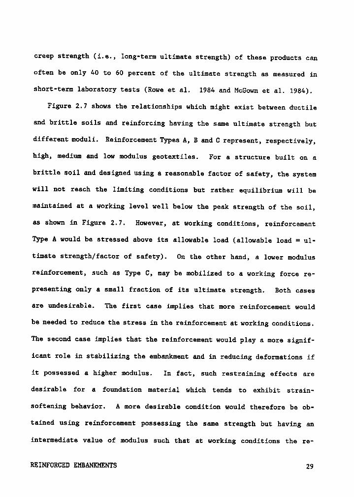
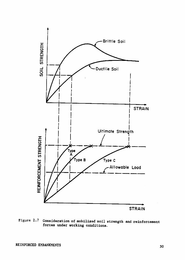
creep strength (i.e., long-term ultimate strength) of these products can
often be only 40 to 60 percent of the ultimate strength as measured in
short-term laboratory tests (Rowe et al. 1984 and McGown et al. 1984).
Figure 2.7 shows the relationships which might exist between ductile
and brittle soils and reinforcing having the same ultimate strength but
different moduli. Reinforcement Types A, B and C represent, respectively,
high, medium and low modulus geotextiles. For a structure built on a
brittle soil and designed using a reasonable factor of safety, the system
will not reach the limiting conditions but rather equilibrium will be
maintained at a working level well below the peak strength of the soil,
as shown in Figure 2.7. However, at working conditions, reinforcement
Type A would be stressed above its allowable load (allowable load = ul-
timate strength/factor of safety). On the other hand, a lower modulus
reinforcement, such as Type C, may be mobilized to a working force re-
presenting only a small fraction of its ultimate strength. Both cases
are undesirable. The first case implies that more reinforcement would
be needed to reduce the stress in the reinforcement at working conditions.
The second case implies that the reinforcement would play a more signif-i
icant role in stabilizing the embankment and in reducing deformations if
it possessed a higher modulus. In fact, such restraining effects are
desirable for a foundation material which tends to exhibit strain-
softening behavior. A more desirable condition would therefore be ob-
tained using reinforcement possessing the same strength but having an
intermediate value of modulus such that at working conditions the re-
REINFORCED EMBANKMENTS 29
Brittle SoilII-OZLi.!
E«> -:1 Ductile SoilO<¤ — . II I
I I II
I I I STRAINI I II I II I Ultimate Strength
E I I IT Type.„ I A
I,. Type B Type CZI-I-I Allowable LoadELIUg ILa.zILUOC
s·rnAII~IFigure 2-7 Consideration of mobilized soil strength and reinforcement
forces under working conditions.
REINFORCED EMBANKMENTS 30
inforcement would be strained to give a high but allowable restraining
force such as shown for Type B reinforcing.
For a ductile and less stiff soil similar comparisons may be made.
Again consider a working stress level based on an adequate factor of
safety. In Figure 2.7 it may be seen that both Type A and B reinforcement
would be stressed above their allowable load and indeed the Type A re-
inforcement would be stressed to the point of rupture leading to a cat-
astrophic failure to the structure. For this case only the low modulus
reinforcement would be stressed to below its allowable load.
It should be emphasized that all three types of reinforcement shown
give the same factor of safety with respect to ultimate limit state.
However, the behavior of the reinforcements is much different under
working conditions. These principles are intimately related to strain
compatibility considerations and are discussed more in Section 2.2.4.2.
McGown et al. (1984) have proposed a procedure to develop the load-
strain curve for materials which exhibit creep behavior which accounts
for the long-term creep strength of the material. This procedure is shown
in Figure 2.8. It consists of determining the strain-time relationship
of a geotextile or a geogrid under a constant load as in a creep test
(Figure 2.8a). From this plot, the load-strain relationship can be de-
termined as a function of time, as in Figure 2.8b, and by extrapolation
the long-term ultimate strength can be determined. Finally, the long-term
stiffness can be determined as in Figure 2.8c.
REINFORCED EMBANKMENTS 31

II(ci „ It
E temg T C II 1 I 1;
[I
[ I-1
', 1 }„ ‘1<
"z<%<Prmx,3I I I 1 r 1} I I 1 [ 14 24 I34 14*5
E 1 '§ I I 1 1 IL7) 1 I I I II I I I [
I ty TZIUTET3 IL Ig gIb) g
p tg T C,„ In
IZ [ IZ'}..¥ __________·____ _ 4,-- sF 1o -- -- .-- -3 1
E ‘ '•| •l
1 ÜE,} E2 E
(C) Str¤1nI°/•ItemcT°C
5)termO ;E ff ·t "“l
Ö EIs
om-, Qt ctraujlgl2 1
.. VI E *IQ2 E1 — ’¤»::9: -1um
T1me(Iog scale} I°9I
Figure 2.8 Procedure for determining load-strain curves for creepsensitive reinforcing materials (McGown et al. 1984).
REINFORCED EMBANKMENTS 32
2.2.4.2 Strength of the Reinforcement-Soil Interface
Under field conditions, reinforcement is subject to pullout forces
and shear forces as shown in Figure 2.6. The strength of the
reinforcement—soil bond at the interface may govern mobilization of this
bond if the shear stresses at the reinforcement-soil interface exceed the
bond strength which can develop. The bond strength which develops can
fail in essentially two mechanisms: (1) failure in a pullout mode due
to insufficient anchorage capacity and (2) sliding of the fill along ei-
ther the upper or lower surface of the reinforcement in a direct shear
mode. The field situations of these two modes of failure are shown in
Figure 2.6.
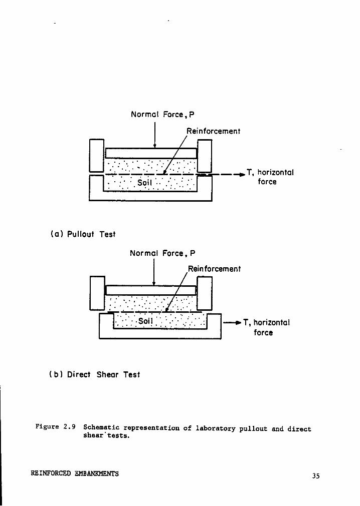
The analogous laboratory test conditions for these two modes of
failure are shown in Figure 2.9. In the pullout test, the two halves of
the box are fixed and one end of the reinforcing sample is subjected to
a horizontal load. In direct shear tests, one half of the box is fixed
while the other half is subjected to a horizontal force. The reinforce-
ment is anchored along an edge of the box to induce tensile forces in the
reinforcement. During each test, the normal load is kept constant. This
results in a constant normal stress:
6 = 7%- [2.10]
where Ab = area of the box. Recording the horizontal force and dis-
placements during the test allows determination of the ultimate shear
stress.
REINFORCED EMBANKMFNTS 33
In the direct shear test it is assumed that the shear stress, 1 between
the soil and the reinforcement are uniformly distributed. Hence, the
shear stress is:
1 = 7% [2.11}
where T is the applied horizontal force and Ar is the area of the re-
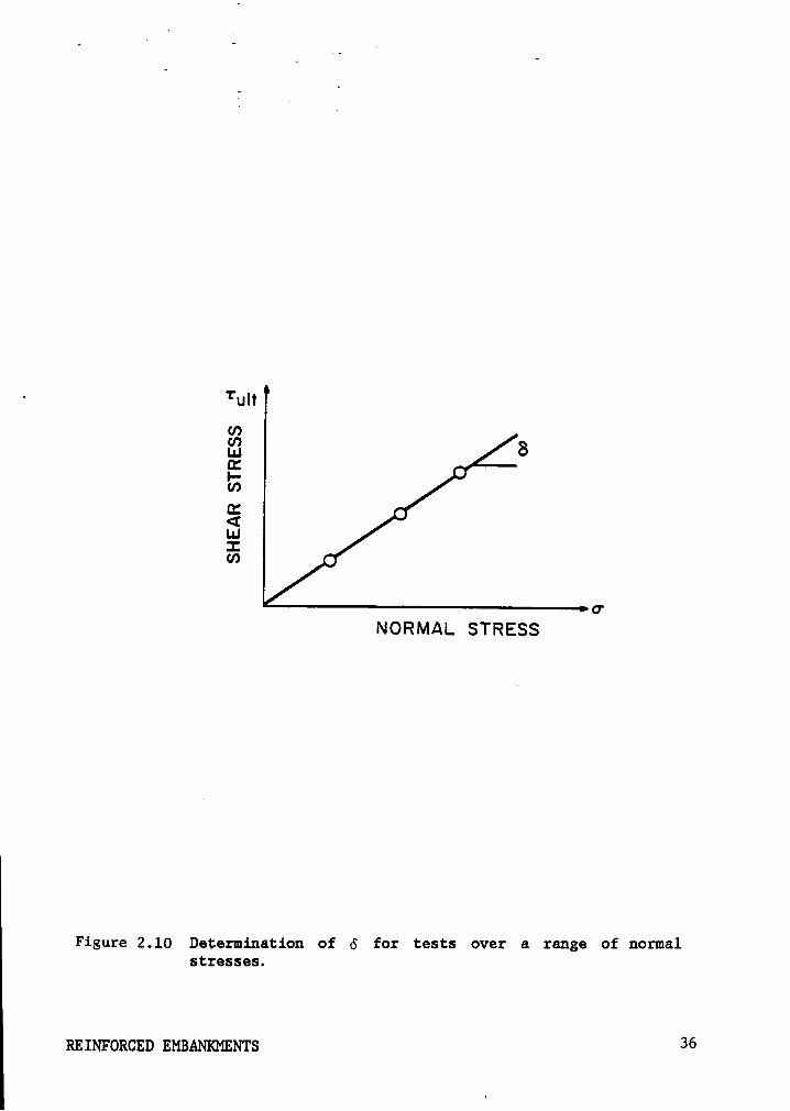
inforcement inside the box. Plotting the values of cuk corresponding to
Tun for a series of normal stresses allows determination of the bond
strength or interface friction angle, 8 as shown in Figure 2.10.
The shear stresses developed in pullout tests on geotextiles are not
uniformly distributed due to the extensibility of the material (Holtz,
1977 and Collios et al. 1980). However, assuming a uniform distribution
of the shear stresses leads to correct values of the average bond angle
of the interface (Collios et al. 1980). Hence,
1 =ä [2.12}
where T is the applied pullout force, Ar is the area of the reinforcement
inside the box and the factor of 2 accounts for shear stress developed
on both sides of the reinforcement. As in the direct shear test, plotting
values of gdn for a series of normal stresses allows determination of the
bond strength or interface friction angle, 8
The mechanism of reinforcement-soil bond is little understood at
present and available test data have indicated it is a function of several
variables. These include normal stress on the reinforcement; soil
REINFORCED EMBANKMINTS 34
Normal Force, P
Reinforcement
Q_..,T, horizontal
. f F force
(al Pullout Test
Normal Force, P
Reinforcement
Q;Q;Soil Q ',; -—-» T, horizontal
force
F (b) Direct Shear Test
Figure 2.9 Schematic represeutatiou of laboratory pullout md directsheazftests.
REINFORCED EMBANKMENTS 35
· Tult
$gg 8EU)
x<ILUIU)
crNORMAL STRESS
Figure 2.10 Determination of 6 for tests over a range of normalstresses.
REINFORCED EMßANr<MEm‘s 36
angularity, density and particle size; ratio of reinforcement opening
size to soil particle size; and relative reinforcement-soil stiffness.
Data by Collios et al. (1980) showed that as the size of reinforcement
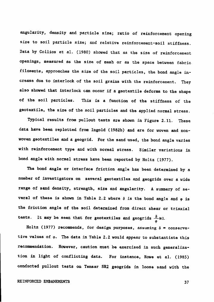
openings, measured as the size of mesh or as the space between fabric
filaments, approaches the size of the soil particles, the bond angle in-
crease due to interlock of the soil grains with the reinforcement. They
also showed that interlock can occur if a geotextile deforms to the shape
of the soil particles. This is a function of the stiffness of the
geotextile, the size of the soil particles and the applied normal stress.
Typical results from pullout tests are shown in Figure 2.11. These
data have been replotted from Ingold (1982b) and are for woven and non-
woven geotextiles and a geogrid. For the sand used, the bond angle Varies
with reinforcement type and with normal stress. Similar Variations in
bond angle with normal stress have been reported by Holtz (1977).
The bond angle or interface friction angle has been determined by a
number of investigators on several geotextiles and geogrids over a wide
range of sand density, strength, size and angularity. A summary of se-
veral of these is shown in Table 2.2 where 6 is the bond angle and e is
the friction angle of the soil determined from direct shear or triaxial
tests. It may be seen that for geotextiles and geogrids éääl.
Holtz (1977) recommends, for design purposes, assuming 5 = conserva-
tive values of ¢. The data in Table 2.2 would appear to substantiate this
recommendation. However, caution must be exercised in such generaliza-
tion in light of conflicting data. For instance, Rowe et al. (1985)
conducted pullout tests on Tensar SR2 geogrids in loose sand with the
REINFORCED EMBANKMENTS 37
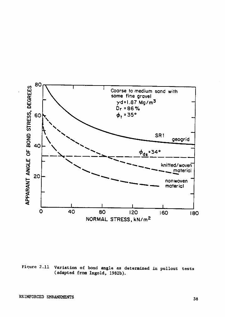
m 80__ uu Coarse to medium sand with
ä some fine gravel8 yd=|.87 Mg/m3Q ÜF :86 °/0
60 ¢t ° 35°LU \E
\\U, \\
SRIgeogridO xca 40 \
‘\u. ¢>ds=34°
ä\\
‘*—_knitted/woven
Z‘\—_
material< $ —
ZÖ iI- *§— nonwovenä *— material50.0..<
I 0 40 80 |2O l6O |8ONORMAL STRESS, kN/mz
Fieuré 2-ll Variation of bond angle as determined in pullout tests(adapted from Ingold, 1982b).
REINFORCED EMBANKMENTS 38
IN_¤
Gc
F;c~
-I-1-1
NI
1:
HI
I-1
IGI)
QI-1
•Q
Q-1
36
.;”'
'6
U
OQ
g-
•0
•-I-1
4-I>
I1
-1:¤
Q0
.O
3·
•-1
:.1G
Gé
GG
•¤
-w~
-1>
VW
NN
0Q
N•
3•••
1-11;-1
GG
GG
1-1
-6-
GQ
·Z
-1*010G0NU
NQ
IBN
'U•
-G
7E
E'T
"'6
.I
EQ
GI
Q3
36
6U
HU
UN
1w
-1-1
;Q
•1
ww
w-1
-1-1
>I
I¤¤
uo
G7G
GU
3-
„G
UG
-1’U
SG
GG
UG
7O
>•
AO
QN
NO
3ca
cc
GN
GIQ
11-1
InQ
-
•6
•-•«
Q-
OG
-I-I
1-IO
OO
O-
-1z
11
1¢
AEEIh
IhIh
ÜW
·O·
IhIh
1-*G
IGIM
FI
IhG
Q1*7
F7F7
Q¢'7Q
IhQ6*7
P7Q
g-
-1N
-Q
OIh
NH
NR
•-
-N
NN
NQ
IhIh
NN
N¢
‘·¢‘·¢
*·¢‘-
IhIIW
IhM
GIQ
Q6'7
NG
IQ
QU
II
NN
AF7
UI-
HH
q:Q
-I-1-1
1-1w
ww
w-1
__G
GG
'¤>
>G
EO
N=
¤¤¤¤
~•·1¤
ww
O1
11
OA
-I>1-
‘G
GIH
IIIHH
-I
GG
GQ
HN
OIB
I!IIIQ
QG
OG
GQ
N-I¤
-1'¤
I-1II-1
··u
mu
mm
-1-1:¤
c-1
•**
E'U
'U'¤
U0
OU
DG
G•-I
wE
Hw
ww
mE
UE
Uu
wcn
cm
w:1
-1-1UI
GG
"G1
'U-G
GG
GG
IIIG
-1Q
o1
-11
-1-4
1·•-•¤
:1:1
11
-1-1-111-
-11.1w
uw
czw
nw
1U
}¢
UG
'¤G
•I-1N
GG
G-1
'UG
VN
GG
>G
G¤
GG
OG
OW
GW
GG
HG
UG
UO
-10
-1
¤I-
IG~
·1¤
UO
EIII
:11
11
1-u
.¤E
uE
U••-eu
11-11-eu-1uu
mQ
-
•1m
•Q
NM
-~
•-IQ
--1
UQ
GU
NG
1-IO
'¤¤
I'G
A>
Q1
-1-1
•I-1
NN
>1N
•1
wQ
NN
NN
NG
NQ
Q-1
wum
ge
m-1
UIQ
QG
QG
Nw
Qw
ww
vu-1
-1w
-1-Iu
-1
¤¤
c~¤0¤~
\ku
m3
QU
GG
GU
GI-1
G1
-1U
QIU
1-I
CA
-IGI
:4¤:
E-U
1-11-I
D*1
zw
-1
results shown in Figure 2.12. The data show a directional bias, and for
pullout, in the longitudinal direction, which is the direction of stress
for SR2, a bond angle of 5 = 18° was indicated. This is much lower than
the sand friction angle of 32°. Pullout testing of SR2 geogrids conducted
at the University of California, Davis (1984b) yielded bond angles of 5
= 64°. The differences in these results are probably attributable to the
density of the sand at the time of testing. The UC/Davis tests were
conducted on a medium grained sand at a relative density of about 95
percent, while the tests reported by Rowe et al. were conducted on a fine
grained sand in a "loose" state.
2.2.4.3 Strain Compatibility of Rainforcamant and Soil
Soil structures incorporating relatively extensible reinforcements,
such as geotextiles and geogrids, are strain controlled systems (McGown
et al. 1978) and hence, there must be strain compatibility between the
soil and the reinforcement at all times (McGown et al. 1984). This com-
patibility is depicted in Figure 2.13. This figure is instructive in4
several ways. First, if a limit equilibrium analysis is performed using
peak soil strengths, the reinforcement strength used in the analysis
should correspond to the tensile force developed at a strain compatible
with the development of peak soil strength. However, as the soil strains
and its strength reduces from its peak value to its residual value, the
reinforcement force mobilizes more force and the overall system may remain
in equilibrium. A limiting condition will be reached only when tensile
REINFORCED EMBANKMENTS 40
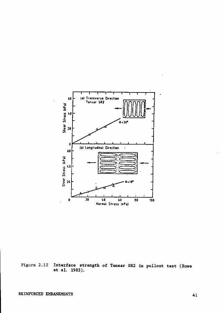
60 la) Transverse Direction 4_· __ Tensar SR2 Z Z; ”
g9; ~•— .Z3
’•°.- ._ g Z
E 20 -°
M
0 IIb) Longitudmal Direction ·60 __ „
:‘°
rlnlbI
gg _A
¢=18°
6Z
20 LO 60 so 100‘ Normal Stress lkPal
Figure 2.12 Interface strength of Tensar SR2 :L¤ pullout test (Roweet al. 1985).
REINFORCED EMBANKMENTS 41
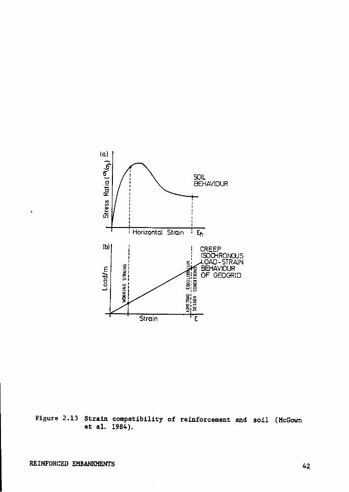
(a)
I
E { SOIL.2 { BEHAVIOURE Q ·an Q Ié’
: Qö { 1
{ :·Horizont¤l Strdin I Eh
Ib) { 5 cmzep{ Q ISOCHRONOUSmg g. OAO—STRA1N
E EQ Z BEHAVIOUR; g: gig OF GEOGRIO3 ¤' ä:§_] EI su:8
äl éieäzä
Strcxin ' E
Figure 2.13 Strain compatibility of reinforcement and soil (McGownet al. 1984).
REINFORCED EMBANKMENTS 42
strains in the soil induce strains in the reinforcement which cause it
to rupture. This argues for the most likely limiting condition occurring
when the soil has strained sufficiently to reach residual strength or
constant volume conditions. Hence, according to McGown et al. (1984),
the soil strength to use in a limit equilibrium analysis of reinforced
soil systems is the constant volume or residual strength.
The extension which Rowe and Soderman (1985) proposed to their BMM
limit equilibrium addressed the question of strain compatibility between
the soil and the reinforcement. A parametric study was performed in which
the limit equilibrium and finite elements results were compared for se-
lected embankment configurations. From the results obtained, a new pa-
rameter termed "allowable compatible strain" was coined. The allowable
compatible strain is the maximum strain that would occur in a geotextile
having a modulus so small that negligible load is developed in the
geotextile at collapse, and it was further assumed that the strains de-
veloped in this geotextile-reinforced embankment at failure would corre-
spond to the strains developed in a similar unreinforced embankment at
failure.
The allowable compatible strain was related to a dimensionless pa-”
rameter Q where
:2 = [2.1:]
where
yf= unit weight of the fill.
REINFORCED EMBANKMENTS 43
Hk = height of the embankment at collapse.
cu = undrained shear strength.
D = depth of soft soil beneath embankment.
Ea = undrained modulus of the soil.
B = width of the embankment.
Rowe and Soderman suggested that in a stability analysis, the force
in the fabric should not exceed that developed at the allowable compatible
strain (i.e., T< 1:aEf where Ef is the secant modulus for the strain range
0 to aa). The relationship proposed between the allowable compatible
strain and the dimensionless compatiblity parameter Q is shown in Figure
2.14.
From their study, Rowe and Soderman found that the allowable compat-
ible strain increased to a limiting depth and then decreased. This depth
was found to be D/B = 0.42 where D and B are as previously defined. They
also found that below a depth of (D/B) > 0.84 a geotextile has no effect
on deep-seated stability thus providing a guide to the applicability of
reinforcement on deep deposits.
2.2.5 Summary of Limit Equilibrium Methods
The following conclusions can be drawn on the use of limiting equi-
librium procedures to analyze the behavior of reinforced embankments on
weak soils.
REINFORCED EMBANKMENTS 44
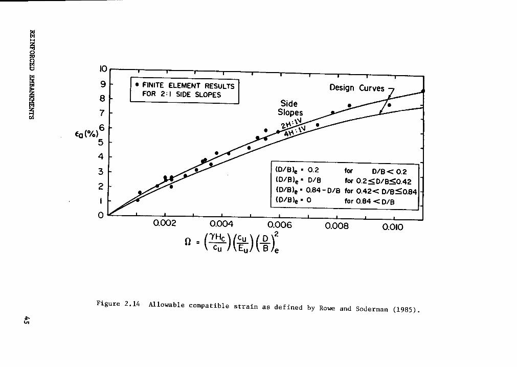
fl
NQ
Q2N
YQ
¤~¤
¤V
I9
Svw
eeQ
U)\Q
Eg
0V
V=—·
Qv|N
q·
Q,=
¤e~t¤=aE
U0
00
<¤§•
•ä
ää
äaa
E'en
QO
°°8
~Q
Qä
mÄ
·M
Nxm
>„O
QÖ
Q.¤
.„gzL-;·;»;·
Eta
'°cn
mm
m<O
··-•--0
1"’ä
°‘B
BB
B8
T5„,„—
¢~
¤~
•¢.(
\]Q
)°¤U3
•QICD
cu¤fi
Y;:»
Elu.:B
x_
zW
__|O
Q•—
•D
m•
QI4
?CE
ßäßO?·~
+-•gg
_II
OZ
0zum
C}EQ
BJm
•N
{Ä[L
IT8
3w
N.
,2:0
:O
'Z:‘E
0u
u.
•E«~i
RCDLn::BP
Q¤
¤m
¤~
co
__
_m
<rm
N-O
rz.äE
REINFORCEDEMBANKMENTS45

1. The use of Bishop's Modified Method provides a slightly conservative
approach to the design of reinforced embankments when a reasonable
factor of safety is specified (i.e., minimum of 1.3 for end-of-
construction).
2. The selection of the reinforcement force to use in design is an im-
portant aspect of limit equilibrium analyses and has, as yet, not been
quantified definitively. The selection of the proper force to use
is a function of many variables dependent upon soil and reinforcement
properties and the geometry of the problem. Until further research
clarifies the issues, conservative values, subject to the limitations
discussed above, will need to be selected for design purposes.
3. More Verification of analysis procedures by comparison to case his-
tory data is necessary before complete confidence in limit equilib-
rium methods can be achieved.
4. The factor of safety calculated assuming the reinforcement becomes
aligned tangent to the slip surface at failure is considerably higher
than that calculated assuming the reinforcement remains horizontal.
REINFORCED EMEANKMNTS 46
2.3 Finite Element Methods
2.3.1 General
Analyses by the finite element method have been applied to reinforced
soil to obtain data on the soil-reinforcement interface, the deformation
behavior under working conditions and as an aid to understanding the re-
inforcement mechanism. Herrmann and Al·Yassin (1978) discussed discrete
and composite representations of the constituents and concluded that both
approaches could be applied to reinforced soil systems with equal accu-
racy. The analyses have been applied to laboratory model studies of sand
(McGown et al. 1981) and clay (Majes and Batteline, 1985) and to field
tests (Bell et al. 1977; Boutrop and Holtz, 1983; Rowe, 1982; Rowe et al.
1984 and Rowe and Soderman, 1984). The finite element method allows
consideration of construction =equence, soil nonlinearity, plastic fail-
ure, reinforcement deformation, soil-reinforcement interaction and de-
formation under working loads. In addition, pore pressure response may
be determined depending upon the soil model chosen. While there are
similarities in the finite element methods used, the procedures vary4 considerably with regard to the modelling of soil nonlinearity, plastic
failure, reinforcement representation, reinforcement-soil interaction,
large deformation behavior, and construction sequence. Table 2.3 pro-
vides a summary of the finite element methods applied to reinforced soil
and reinforced embankments. To date, no method incorporates consol-
REINFORCED EMBANKMENTS 47

idation analysis and pore water pressures explicitly into the analysis.
Several applications to reinforced embankments are discussed below.
2.3.2 Bell et al.
One of the earliest finite element analyses of reinforced embankments
over soft, weak soils was that performed by Bell, Greenway and Vischer
(1977). The authors analyzed a geotextile fabric—reinforced rockfill
built on a 10-ft thick peat deposit in Alaska. The fill was modelled as
a linear orthotropic elastic material, the reinforcing as a truss element
capable of transmitting axial force only, and the peat was modelled as a
homogeneous, isotropic, elastic-perfectly plastic material. The authors
analyzed three cases representing embankment dead load only under condi·
tions of no reinforcement and single layer reinforcement and the case of
live loads (representing haul trucks) on the single layer reinforced
embankment. The analyses showed the reinforcement to have little effect
on ultimate settlements, the reinforcement stiffness to have no effect
on settlements and that fabric tension increased with increasing fabric
modulus.
The authors made the following main conclusions: the main function
of the fabric was to prevent local bearing failures, thus holding the
embankment together and causing it to act as a unit and when shear fail·
ures do not occur, and embankment settlement was essentially the same in
the reinforced and unreinforced cases. It should be noted that this was
one of the earliest cases of embankment reinforcement over soft soils and
REINFORCED EMBANKMENTS 48

A_
;
·C
IN
IF
Iy
QL
CI
II
IC
0~
!~I
0nl
ud
CU
Ü·I
Uu
lIJ
0*
QU
hu
lbU
I*
GU
Cu
Cd
IC
1:
dL-
0*0
CU
L-
Iü
ßI
I!•
Ü}
*0
be
bla
!d
ßN
EI
dU
CC
*}
H-
CD
Uhe
VN
NA
Cd
h-
Hl
N>
CIO
IIN
Id
Id
lI
NI
II
·II
UIII
CC
U0
}**C
UN
IE
IH
CN
ld
.Q
--1
Q.
gyn
un
sl
lu
bd
IU
N*U
*\!
0>
•!
N¢
dlb
0l0
•*,§
dI
INI
lld
ld
zß
*II*I
CI
•¢I
llG
UIIU
IC
IQ-
IGn
!I|
na
nl
L10
Id
du
L!C
uu
Qß
ldh
ldd
LI>
IU
nd
dC
>t!
UC
Id
!d
n-u
dC
UI
lg
•1Q
.0
a•ld
CII
Cd
0U
I-I
III~
UIL
-{-1
0••
I2
VII
5lll
IN
UIII!
IC
vI7
¤·1
L-u
hA
L1
•0
•°•«
0U
·I
n4
·I
CY
-0
Il
II
CIII·U
N¤
IÜ
U•'IIU
UIJ£
~lU
\1
NH
Hu
U*l—
Il§1
dIII
SIC
IUN
UIIO
••U
hlU
dl
••nlN
C0
C-¤
CC
ICß
lü
ll-0
90
lII}0
NC
ß>
‘¤
lIII
NO
Nd
ߢ
·•11
¤••1
|d
ld
Na!
NU
Clu
-d
dIZ
§0
I1
IIU
IIU
CC
00
0¤
•I•!N
AI
dt)-¤.CC
dL1db
laI
NI¤¤¤
III
II
IN
OIC
III
**
uzg
u0
II·•¤
|I
•¤
)Iv7
~*
·*U
CO
II
II
Usl-!}
C°!·
Qu
!‘d
|ll§1
lAI
B-C
IMI
llINd
NlN
L-I
UI
UI
•'
OC
C•¤
¤N
Ut!*0
dN
ud
dd
H>
;•!U
Il§
H•l§
HI0
UId
IC
N·
IÄ
JC
GIV
NU
II
HU
NI
dIC
NC
Cd
UIN
•!l•
llChs
F1N
a!
dIII0
ldH
IO
HIC
CIO
!-n
dd
lb
dIO
C'·¤
0C
3|N
•!L
•2
Q•1
>,u
••;n
•u
uld
uu
lu
dln
¢d
u!A
•-•!•
>d
dlI
NO
I0
l|*0
!•
H•·•§
IN
ÜIC
uu
!'•·*C
NIU
II
IIU
-D
CIIC
IC
II
II
I*l§
1U
UB
Cd
Elü
ldd
dd
Cd
I>~
ÜIIA
UN
IIdd
:d§
•lN
dN
IIN1
CU
CIC
•-d
l!
BÜ
l•'•III}•·•
CII
IIN
Uh
!G
UU
IIIIN
V•1
Q•¤
•N•1
¤•ld
UIC
CIN
IIN
dU
-K
WY
Id
Nd
IG
-Ulu
h-1
Lb
Na
!Na
!UC
IN
ll0
*III
$•!I!0
00
§I
NIIO
IB
IJC
ÜU
NH
CU
Z]*
<II§
1Q
§•l)
L>
III¤
|Z
II
Dllü
lld
llvlß
db
dN
B•·•
N-1
N-1
N8
4J\
:9GIU
U(N
I;U
tu
CU
v!
U!
·-•&
¢U
L-•-¤
·Cß
•I
00
UIh
dN
S->
2C
10
dä
bi
v'
•-!C
dIV
IN
CC
a!
I§
l¤·
C2
l0
IC
E>«
II
Id
kI
NU
§•L
-U
V!
C0
•·<I
0C
00
*7
II!
dl
alIl
d>
«I•
•!U
0Il
Nl
du
:C
NW
ild
•n
•u
----0
0U
n.:
Ul
nll
0451lC
>n
‘G¢!¤
dC
lßd
dl!
•*
UE
UN
·-1L
-lll
Id
GI
JN
CI
NN
DS
NG
IU
IB|••
nm
-1
äI
B=
tn:
1-0
CN
Ü0
C0
I*'*
AII!
Au
>V
UI
ln-1
$[1
1Ü
II
UO
}I
IION
:€
"2
;*··“
">
••-I!
NII
AG
CA
IA
OL
!0
VU
L-
0u
n*
S0
•·§
-¤•
--3
E3
*-2
"'-“
£"‘
IIh
IIO
III
IO
II
I7
-72
*>
->>
•I¤
0äA·
*L
A;
gL-
0•u
:•
••¢„‘,‘j
AC
1u
un
UV
Ig
z:
_g
u-1
1-·«
¢7
·*8
*0
2;-
AB
5ld
un
dA
UU
1:1
~a.-.-
-1
>1
·o¤
v¤
-L
s,
L3
-•->
„-·
-¤
•·
····=A
,.A
,.s
av
··~•-
¤···
¤•·‘
""
AA
.--
¢°
*“
"i""
°'
6-;.
un
o••
°°
“'
°„:"°3'
2‘;3•—---••—
-L
-Ihn
I•"
"'
=-·
•·-·:g
::
Ev:
Jä
äiä
nn
II
*"
•g
—s
ulu
ua
Ag
gv
ulu
uß
UV
I
C
1·-
7*5
ng
he
ld
!n
uI•
C;
an
-g
oa
-e
c1
*·'•
·*‘
na
n-
¤-::•¤
u1
os-u
«•1
u~
—¤
en
¤¤
I“:
•¢
:•s-
un
s-
ce
olu
väcs-:
1•--••-u
va
cL-
-•-¤
•-u
u-1
-«·
:—-
1••-•o
u·
••
·u
va
ux
•>—
na
u¤
nu
nn
big
:0
0••
uu
1o
—•—
:u
7_
ug
nc
VII
CId
C°
-•|l}N
>•IIC
9IS
V-••1
u
<¤
«—
1u
uu
3A
•W
läb
uu
‘nu
ug
gC
I<G--N
IIIIH
"U
:IZ
HC
N_
.•
A0
•1u
=_
•*IZ
Cd
Iu
vn
vo
n-
:¤
•-|
••
ye
¢·
UN
"‘
Eg
•°:cc
UI
g=
Q.
gg
UN
7**
‘2
l2
:23
2:
-1n
lV
{I
••\l
4-1
GI
QA
'.2
21
;.---e
xQ
Qa
a~
IN
d·
NU
IC
I}*
CI
IA
IIII
I~E
0IIG
I•N
Id
ä•-1
INC
I;H
Qd
10
lB
gld
gl
NO
UIä
0**
Qu
aH
LZ
¢Z
=lv
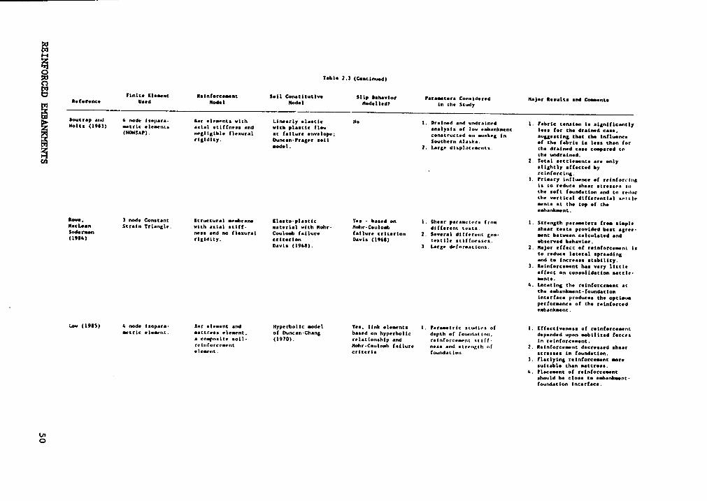
¢U
I••
IÄ
CC
-II
'•‘'
eL
·-C
1.:
ey
lgU
I6
uIG
H-b
nr
ll-nl
I-•nl
gv
CI:
HU
Cg\¤•C
HH
lIN
C•-n
lI
IS
UI
IC
Ill
GI
IvIE
*NU
evu
llI
InU
•;C>~
EG
GI
C·•lI
nlU
LIG
CU
•¤
IIG
-•C
Il•-
UI
I•*Ä
•*I
CC
LG
UN
I8
Q\¤
|I•·•CI
C•¤
II
gl
0GU
•¤•:0
QE
LI
••I§
IU
LI
\•Ig
vI
IG
|~
•I•'
C•·•
CG
G
G~
U·‘|
UC
IC
IL
Lu
tM
BI
GI-
•Ä
GIU
I~
¤§
lIIC
CII
el;
lU
|¢n
lIl
Uh
nL
•«
\•<
VIII
CU
IGIu
i.
-•¤uns
n>„e
u•
GI
¤¤
A•~
l~•'2~l¤-
•--••-•‘•
••••
IE
II
IBI
Ch
vIh
vvII>
II
I-•IU
IBG
UÄ
¤*U
LG
II
\¤
G,'I
UG
\¢
JlI
Lv
LIO
U—
GI
lvl
IGII-lä
dI·<
0L
Lvll~
•C
GIC
B·U
GlllC
UE
U•¤
III
UI
gü
nlä
lßU
>•**G
IIF
!-•*IU
n|
¥¤
sn
|ICG
vL
LU
••IG
u£
I•‘G‘G
I•¤
\Il•I§
GI•I
GC
GB
NC
IIIC
GI
I•
0IIE
GU
l¤U
>G
III
LU
GIA
IlG
CL
IMC
GC
UIIG
II
IIß
In
lInlC
CG
IIC
IU
EvC
GC
I•¤
II|·<
IIl¤
·•-Ilvü
LC
ÄU
IIC
GIIL
IG
IC
II§
l¤¤
•e
I«CL
GC
•«h
•Nn
¤•\lG
I§·
IIIIU¤
-ha
llC
-!G«
I·IÄ
UIC
HIG
UI
CU
NB
I·¢
UIC
CB
h•U
UU
GIU
IB
IU
UU
hl
CIL
Iv
UQ
UI
CIC
IU
e•G
•¤C
II
NIC
IC
CIC
CI
GI
NU
IGe
IU
UU
CIN
G\¤
U•*U
GN
IU
I>
G§
•\lIC
IC
B··¤
3a
un
gn
nu
xu
nu
ei
uu
•••¤
n-C
AIII
·•••:•••••-«u
IU
NIIL
UG
LG
IN
B:
GG
GU
~-¤
I\l\•-IU
g~
¤•G
IÄB
IGI
I••
IC
GI-•C
\¤
•IG
I>
IC
Cl
BIU
NU
IU
IL
GC
UI\¤
I•·«
II-n
IL
I=U
INC
IUU
IIIU
IGH
CIlI
IEI
IIUC
IUU
UIE
I€
2¤
—Z
£ä
:1Z
„¥!‘€
¤2
‘3?
¤2
1Z
‘“2ä
1€
C“¤
“:"
‘°’
GI
··
~-
·6
„.
„6
.E
¤•
Nß
•-
NF
!n
l•~
•M
FQ
4
C
GC
NI
IE
III
·C
¢I·G
CC
]I
LQ
I·
:e
:I
eIl¢
uE
bvll
un
ßs-
LII'
Cu
l:
ge
e;
•e
Ü-:
••·:¤¤
6.-.,....G
GI
IL
Ih§
~•-
TIM
E••>
•C
IC
-lb
Inl|~
Cn
|IG
CIG
5-G
IU
UIIE
In
lCn
«&
C!
II
IIE
EI
IC
C;.
Qu
EN
GE
-¤
|-«
Ee
LG
IU
6U
ÜG
II}
Ivn
•G
UE
IIC
••'•C
-1ä
E"""
""
°h
l1
:-·:C¤
so
-u
a:::2
:In
ZIL
IL
In·¤
GII
ll>
«lC
IL
I\•••l,
IL
L-
Qe
e-IU
NIvI•lN
IU
CI2
eL
ßvlä
BIU
ÜJ
ÜG
ÜU
JI
Iv
Iä
66
6-—
¥¤
¤'§
:.‘21
°2&
·“G
II
Ilt
gg
gI•••
IA
UO
JIn
x"
I!
•-C
CC
III
BG
IV
vG
GG
e•'
GU
LE
-«
9L
UB
G••C
Iq
ne
bC
vl
La
ne
GII-n
ge
UÜ
GIG
II
IIIG
Lv
za
zn
-¤
I
Ixn
-L
•-:6
-•A
IU
•*G
I"‘
)e
vtl
[Q
IN
e•l§
¤>
UI!
GC
Ul
Cl-
•¤C§
·S
II
IIIII
Un
l•·«an
EU
ee
Qg
ee
QU
es-
IU
II
III
OU
·U
IIL
L—
§¤
CG
•—
CIG
ÄIIL
Gu
-G
el
•-I
-n
un
-•«
I;
ee
Gz·
8l
••ß•-:~
an
ge
AA
III-:
un
II
0A
•¤•
UG
IU
§•«
>Q
0••
ee
ua
ßl-IG
LI
>•E
„-
l:JII
IK
ICU
UC
EG
V
Il'!
CL
LIL
(n
g••
nlE
LE
IV
"vll
ilull
2C
vU
III
ee
IG
CI•¤•
‘UE
IIIUIC
EI
OlC
JE
°U
•-I'
•-•c¤
•-.-:
co
n}
ug
uA>~
n-g
nIn
uv·
GU
lvu
ZI
nl
IIC
LU
H!
-n
n-
un
a-
-0
:.:::
Clv
-•G\l
GIh
lva
eI•-e
Illu
UC
CI
L••N
NL
UIN
LU
V-•I
BIllß
vu
eg
eII
ke
IIC
LIII
HN
CIL
I
.6-¤
ue;··
CI-l
Ce
-In
l
IZ
:'ä
ZSI
ZI
II
LI
eC
IC
vG
I“2
:1:
°::1
ss“
°..
ää
äIE
I:
BS
LS
IG
LU
LC
eV
FU
III~
1I
I
2I
gd
A
2'2
,"‘
IL
vC
LI
(E
au
lI
hlt
•Q
EIn
UU
JIN
:6:
Z22:·
IE
ßlß
lv
the fabrics available at that time were much less stiff than those
available today.
2.3.3 Brown and Poulos
Brown and Poulos (1978) used an elastic-plastic soil model (Davis,
1968) to analyze the collapse height of unreinforced and reinforced
embankments on stable foundations. The reinforcement was represented as
a member possessing zero flexural stiffness and as carrying axial tensile
forces only. The results obtained for cohesive soils are shown in Figure
2.15 in terms a stability number ;¥;£ and the percentage reinforcement pr
in the soil mass. (The percentage reinforcement is the ratio of the
cross-sectional area of the reinforcing to the cross-sectional area of
the embankment.) It can be seen that as the amount of reinforcement in-
creases the stability number increases and hence the height to failure
increases. Brown and Poulos showed that increases in stability of up to
40 percent were possible using reinforcement. Brown and Poulos also an-
alyzed granular frictional structures. Here the results of model re-
taining wall tests performed by Lee et al. (1973) were analyzed with the
results shown in Figure 2.16. The finite element results shown provide4
a better approximation to the model test results than the Rankine method
proposed by Lee et al.
2.3.4 Jonas and Edwards
REINFORCED EMBANKMENTS Sl
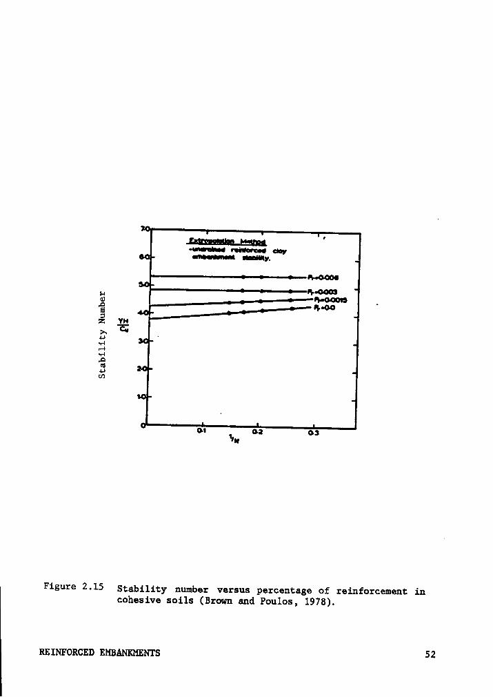
I•u•¤!ü•••
••iI¤•·~e•• d•ygg •m••u•••m
uniuny.
H·•0®l
Hgu'
Z YH
ÄH
H '•1-I•—4•v-4•¤<¤ .H
U1
· 0-1 02 Q3YH
Figure 2-15 Stability number versus percentage of reinforcement incohesive soils (Brown and Poulos, 1978).
REINFORCED EMBANKMENTS 52
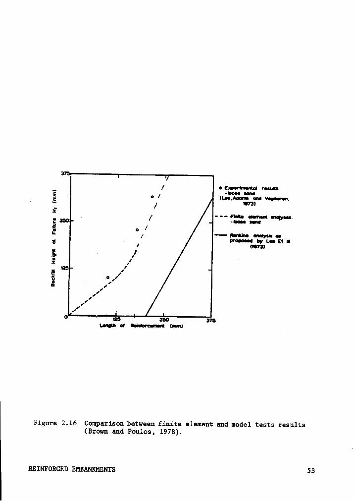
o Exa•r•m•mu r••u•u
E ¤ / (L;•,Ana::M¤¤ Vognann,‘ ~• / $73)f ··-• FHM aanan unjysq.,; Z50 sauä • ’
. ./
·—-kun audyus
•.5 . /¤•·~••¤••em:;,L•• ze e
I .1us {§ . „xB
;’Ill
Il1,1
° · us 250 :7sLaßh ol I•i••a·e•·n•¤ (mm) g
Figure 2.16 Comparison between finite element and model tests results(Brown and Poulos, 1978).
REINFORCED EMBANKMENTS 53

•.i—,é%§;·äFront face ot watt '————-1|————•Po•6tiv• •ngt•
dl rotatton r-—?—gt·—··————-I•i-———-I
(a) ssmvtmm an eur-euer m:«·t•t mum
Fwflt flcoof1
N•gatlv• angte 'ot rotation
_ 1—.- * ;
l I EI .
soft(b) Behavior ofa ad!-i material ayatem
Figure 2.17 (a) Behavior of a stiff-stiff material system (b) Be-havior of a stiff-soft material system (after Jones andEdwards, 1980)
REINFORCED EMBANKMENTS S4
Jones and Edwards (1980) employed a nonlinear elastic soil model to
analyze reinforced earth walls over stiff and soft foundation soils. The
results of parametric studies showed that a reinforced wall over a stiff
foundation (i.e., a stable foundation) would tend to rotate about the toe
with an active mechanism away from the fill as shown in Figure 2.17a.
On the other hand, a reinforced earth structure built on a soft foundation
would tend to rotate back into the fill as a rotational slip develops
through the fill (Figure 2.17b). These observations show that conven-
tional design procedures for global stability based on overturning about
the toe may not be applicable to reinforced earth structures built on soft
soils. The study also showed that design methods for internal stability
of the reinforced soil were independent of the foundation strength and
need not be altered for soft foundation conditions.
2.3.5 HcGbwn et al.
McGown et al. (1981) used a hyperbolic soil model and bar elements
representing the reinforcement to analyze laboratory model tests of
geotextile reinforced sand over rubber (to simulate soft soil condi-
tions). The analyses were limited to working conditions with no attempt
to match failure conditions. The finite element results showed excellent
agreement to the model tests for settlement and horizontal movements
demonstrating the applicability of finite element analyses to workingl
conditions. An interesting point from the finite element results was the
need to use reinforcing properties based on in-soil tests rather than
REINFORCED EMEANKMENTS S5
those from unconfined tests in order to obtain reasonable agreement with
the model tests. In-soil tests of the reinforcement allow rational con-
sideration of the effect of confinement on the reinforcement-soil system.
2.3.6 Boutrop and Holtz
Boutrop and Holtz (1983) extended the work of Bell et al. (1977) by
incorporating the Drucker-Prager soil model into the analysis and con-
sidering undrained and drained conditions. The results indicate that
reinforcement has little effect on total settlements but does reduce
differential settlements across the embankment surface. Comparison of
the drained and undrained cases showed that reinforcement tension was
significantly less in the drained case. The authors felt this showed that
the influence of the reinforcement on embankment behavior is much less
in the drained case than in the undrained case. Another interpretation
may be that the reinforcement force will decrease over time as the be-
havior of the system changes from that of undrained to drained conditions
and the drained case represents the minimum amount of reinforcement nec-
essary to ensure acceptable long-term performance. Comparisons of stress
levels in the unreinforced and reinforced cases showed that shear stress
levels in the foundation were considerably reduced by the presence of theb
reinforcement.
iREINFORCED EMBANKMENTS S6
2.3.7 Rowe and Colleagues
Rowe and his colleagues at the University of Western Ontario in Canada
have performed extensive analysis work using the finite element method.
The approach they have taken is based on a plane strain, elasto-plastic
soil—structure interaction technique described by Rowe et al. (1978).
The soil is assumed to be an elastic-plastic material with a Mohr-Coulomb
failure criterion and a flow rule of the form proposed by Davis (1968).
The reinforcement is treated as a structural membrane having axial
stiffness but negligible flexural rigidity. Slip between the soil and
reinforcement is assumed to occur when the shear stress between the two
reaches a limiting value based on a Mohr-Coulomb criterion. A detailed
description of the formulation of the method was provided by Rowe (1984).
Rowe (1982) analyzed the Pinto Pass test section (see Case Histories
in Section 2.4.3) using the above analytical procedure. Due to uncer-
tainty in the published soil and geotextile properties, a limited
parametric study was performed to bracket expected properties. Both
drained and undrained analyses of the test sections were performed. The
undrained analyses showed relatively small settlements (0.05 m) and small
fabric forces (0.4 kN/m). The drained analyses showed much larger
1 settlements (0.5 m) and fabric forces (2.3 kN/m). An analysis in which
undrained strength parameters were used with drained modulus parameters
showed results of 0.6 m of settlement at the centerline and a maximum
reinforcement force of 4.4 kN/m. According to Rowe, this type of analysis
(mixing drained and undrained parameters) provides an indication of un-
REINFORCED EMBANKMENTS 57
drained stability of the embankment as well as providing an upper estimate
of deformations without having to resort to a consolidation-based analy-
sis and it provides a sufficiently accurate and conservative answer for
practical purposes.
The effect of fabric stiffness on embankment behavior was studied.
Increasing stiffness had little effect on settlements; even using an ex-
tremely stiff fabric reduced settlements less than ten percent from the
unreinforced case. The major effect of increasing fabric stiffness was
to reduce lateral displacements. This reduction in lateral spreading of
the embankment results in greater confinement of the underlying soil which
reduces the extent of plastic behavior in this soil. For relatively low
fabric stiffness, relatively large deformations can occur prior to the
fabric reaching its ultimate tensile strength and for all practical pur-
poses, failure may be deemed to have occurred prior to rupture of the
fabric. This implies that the stiffness of the fabric may be as important
as the tensile capacity in stabilizing embankments on weak foundations.
The analyses also showed that sufficient fabric anchorage can be
mobilized without overlapping the fabric at the embankment edge, as was
concluded by Haliburton et al. (1980) from the field data. Also, con-
sideration of the fill stiffness showed that increasing the fill stiffness
enhanced the role of the fabric, thus increasing fabric stiffness has a
slightly greater effect on deformations for a stiff fill compared to a
loose fill.
Rowe et al. (1984) analyzed a geotextile-reinforced embankment con-
structed on a peat deposit using the above described techniques. Input
REINFORCED EMBANKMENTS 58
parameters for the peat properties were determined from direct shear
tests, triaxial compression tests, uniaxial tension tests and simple
shear tests. The results from these tests yielded very different values
of ¢'and c' as shown in Table 2.4.
The properties of the geotextile used were determined from wide strip
tensile tests which provide load-elongation curves from which the tensile
strength and modulus can be determined. Two types of geotextile fabric
were used to reinforce the fill: Geolon 1250 which has a coarse and
relatively loose weave and Permealiner Mll95 which has a fine tight weave.
The Geolon fabric had an intrinsic "slack" in the early stages of loading,
often referred to as offset. Because of this behavior it was necessary
to assign a lower modulus to this fabric during the early stages of
loading in the analysis.
The effect of using different shear strength parameters was investi-
gated by comparisons to the measured field performance of the embankment.
Using strength values from field vane shear tests produced calculated
settlement profiles which did not agree with the observed results. Ana-
lyses performed using remolded vane shear strengths predicted collapse
to occur under fill heights of 1.5 meters, which did not occur in the
field.
The strength values from triaxial tests underpredicted the settlement
and lateral deformations. The best agreement between observed and cal-
culated deformations was obtained using parameters from simple shear
tests, which were very similar to parameters from direct shear tests.
REINFORCED EMBANKMENTS 59
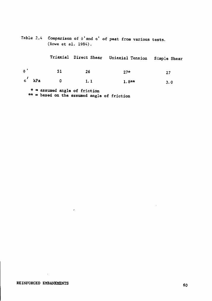
Table 2.4 Comparison of d>°and c° of peat from various tests.(Rowe et al. 1984).
Triaxial Direct Shear Uniaxial Tension Simple Shear
q>' 51 26 27* 27cl
kPa 0 1. 1 1. 8** 3. O
* = assumed angle of friction** = based on the assumed angle of friction
REINFORCED EMBANKMENTS 60
The analyses by Rowe et al. showed the viability of using finite el-
ement techniques to model reinforced embankment behavior. In addition,
the following points were made by the authors: The major effect of the
geotextile was to reduce lateral spreading and to increase stability.
Even a high modulus geotextile will have little effect on consolidation
settlements. In the design of geotextile·reinforced embankments, con-
sideration needs to be given to both the strength and modulus of the
geotextile. The modulus will usually govern the selection of a suitable
reinforcement material.
2.3.8 Low and Duncan
Low and Duncan (1985) developed a composite soil-reinforcement element
to model the behavior of foundation mattresses, which are composed of
geogrids and granular fill. Through superposition of the stiffnesses of
the reinforcement and soil, in effect, a new material is defined. An
important assumption made here is that no slip of the geogrid relative
to the soil in the mattress can take place. This assumption can be called
into question in light of the results reported on geogrid·soi1 interaction
in Section 2.2.4.2.
This mattress element was incorporated into a soil-structure inter-
action computer program (SSTIPN) which uses the Duncan-Chang hyperbolic
soil model (Duncan and Chang, 1970) and has bar, beam and interface ele-
_ ments. Parametric studies were performed of typical geogrid mattress
1 reinforced embankments and embankments reinforced with flat·lying re-
iREINFORCED EMBANKMENTS 61
inforcement (represented by bar elements in the analyses). From these
studies the following conclusions were reached: (1) The effectiveness
of reinforcement in restraining embankment and foundation deformation
depended upon the magnitude of the mobilized force at working conditions.
The greater the mobilized reinforcement force, the more significant the
reduction in deformation. (2) Mobilized reinforcement force increased
with increasing stiffness of reinforcement and with increasing foundation
depth, while it decreased with increasing foundation strength. (3) In-
creasing mobilized reinforcement forces decreased both shearing stresses
and the extent of plastic failure in the foundation. (4) For embankments
constructed on weak foundations, flat-lying reinforcement appeared to be
as effective as an equivalent geogrid mattress. The flat-lying re-
inforcement is also much easier to construct. (5) Placement of the re-
inforcement closer to the embankment—foundation interface was slightly
more effective in restraining deformations.
2.3.9 Summary of Finite Element Studies
From the finite element studies described above, the following con-
clusions can be drawn concerning the behavior of reinforced embankments
over weak soils.
1. The major effect of reinforcement is to reduce lateral spreading and
to increase stability. This is accomplished by reducing shear
stresses and plastic flow in the seil through an increase in con-
REINFORCED EMBANKMENTS 62

finement pressure in the foundation soils due to the presence of the
reinforcement.
2. Reinforcement has very little effect on consolidation settlements,
but it does tend to reduce differential settlements at the top of the
embankment.
3. Increasing reinforcement stiffness decreases the extent of plastic
failure in the foundation soils.
4. The optimum location for placement of the reinforcement is at the base
of the embankment.
5. Shear strength parameters from simple shear tests provided the best
agreement between calculated and measured behavior.
2.4 Case History Performance
2.4.1 General
Several full-scale embankments have been constructed to demonstrate
the effectiveness of reinforcing to improve the behavior of embankments
on week soils and the observed results of these trials provides much
T useful information on their behavior. A summary of reinforced embankment
fills constructed on week soils to failure is given in Table 2.5. From
Rzmrokczv EMBANKMENTS 63
this it can be noted that many of the fills have been built on peat or
very organic clay soils.
Few of the reported case histories provide adequate details of the
reinforcement properties, fill and foundation properties, measured re-
inforcement forces or descriptions of the analyses performed. In many
cases the benefits accrued from using reinforcement were evaluated from
qualitative field observations and from comparison with similar unrein-
forced construction. Cases that do provide detailed information are
discussed below.
2.4.2 8611 et al.
A field test of a geotextile-fabric reinforced rockfill constructed
over a 10·foot thick peat deposit near Petersburg, Alaska was reported
by Bell et al. (1977). The peat was a fine-fibrous type eight to eleven
feet thick. The shear strength, based on two-inch diameter field vane
shear tests, ranged from 50 to 350 psf with an average value of 250 psf.
The fabric was a nonwoven, needlepunched, spunbonded polypropylene having
a tensile strength of 800 to 900 lb per foot for an elongation of 100 to
200 percent. The geotextile was instrumented with simple open/close
electrical circuit strain gages which could record a fabric strain up to
50 percent. Settlement plates were installed to record the deformation
of the embankment.
Test sections having no reinforcement and single and double layers
of reinforcement at the base of the fill were constructed. No obvious
REINFORCED EMBANKMENTS64
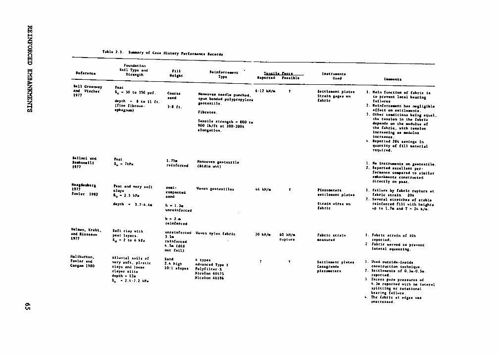
•.1
6•.
..„
'Jnn
Ian
II
In
5-I
j3
ean
A-;.
•e
••Q
qh
s•¤¤
Ue
IA
QI
uQ
QI••IG
II
Iln
I••\
VI
HI
9;
Antn
IG
~••
I••¤
QI
UIJ
G-4
5In
---
Ie
e¤
·Q
AIn
•d
l:U
HII
UIS
II-
II
hh
QIG
IIII
III
UB
-1>
IOIO
CI
AI
sU
eI••n
GI
IUIB
IUI
IILN
UI
Y-
IGI
II
GI
II-!
QI
QU
IM
OIU
QH
I-•I
Inv-
IN
AIA
IQ
UI
GI
UIn
0••I
•nB
-Q
GH
Ill!
U•|
gs
*0-•
::Iu
·un~
••2I
eg
-•-1
~o§•¢¤•
IIIU
I:
>•·•O
IIIUnt
Iln
hnIG
IUQ
Ieu
-Q
°'
·‘¤§
¤•S
22•."-S
25}S
*52°
“1.'5
3..
:*2
3*
'‘:
““"""’2
"‘‘é
'2°°‘
.15
23
;‘
*32U
BIIIG
IhI
>I
QO
IIU
¢••
-U
HIG
OQ
·N
0IU
UI
äI•U
QI
Hln
?e
en
hu
IUQ
UG
IG
:e
Ie
GI
•G
AU
IIN
u·II
IU
G-¤
IQ
h•••I
GIIU
III
5•••IQ
>-Q
HQ
I>
•I
0•
IQ
IU
UIQ
BB
GH
II>
I5
•IG
IA
IIIU
IU
IU
•-•I
-n
n-e
I¤¤
IIII
I·•¤
UA
¤Q
QIH
IUI2
IIIu~
•¤\¤
IU:
UI•
uI¢
UU
UI
IMIU
IIUG
II5
•Ih
•U
5n
u§
•II5
•u
eG
5-IG
0I~
•h
h¤
•I
eu
er-
we
nn
-n
ea
-n
n¢
§•n
GII
IH
MO
GI
••0
lII
•-M
IG
Ul¤
0l•
IQ
IU
I\n
I•«
hU
"‘°":‘3
z°*£
¥ä
%§
$-2*6%
-‘¤2
*32
1-.
*22**3*3Z
JN
IQ
|~§
•vI\¤
IIn
-n
lne
¤u
vIh
\•I~
!IA
EI
AA
AJ
.-JAA
A..§
A.i
AA
J
:§•
cn•
...„
·—„
EE
GQ
‘:
Is
II'2
27
223
.„g
ä-
5;,
.-“;
**2
2E
":-.
EcoS.
Gu„.
...gIa
ne
e~
nI
~Q
•*"""'
un
•h
hu
un
s¢
“"‘
•¤a
na
nu
ne
•'•“"‘
•••u
n0
0••~
··*“'
Inu
un
na
us
UIIlI§
•
IßSE
‘.•
•—“
_,g„,S
0%
l-a
n-
QI
I\
·[
S:5
~‘
¤5
52
2"
4Q
IN
II
6E
“Ia
n‘
:>.
8•
BD
EI
‘
~IB
n§
ZU
GB
GL
•e
q_
I>
•IS
UI
U,
IIn
-•U
Ie
:•
°°'
MB
IIU
II
I>
-IQ
·\¤
I·
In
-g
Q§
•InG
I0
UG
Q4
U•.
¤·¤
-•
-°
°""°'°
‘N
I4
0·-
In
ßt
0—•
::~•
nn¤
~·•
GI
nn>,
g.,
UI
IIU
II\U
IQ
GII-«
GG
•I
>.e
¤n
-•,¤
••
>I
0I
I•*•·•
Q0
*G
GB
GB
-u
nE
GU
hI
GE
QII
II>
-I>-II
IIB
AG
SI
e>
>u
>•-•u
u2
OB
In
lI
anIl
I0
QIe
•-
.zu
lIn
•·0•
lvJ
Ja
<¤
•zzI*•
¤¤
°•
•n
*•I
uvs
1:=
:2
.:.·:E·2:
„='*I-
U·
InU
nu
[5
-$
1sie
$2
•-ll
IU
OU
·G·0
G¤
~4
I•I
>-
¤n
QI
he|h
••|
ae
Ne
eIn
heg
ne
ele
'!4
5G
•-ll
IG
IlG
|{
un0
In-•
IG•
n~—•
IE
Ih
-•n
e--
US
II
¤·I
III
G·I
gn
I5¤
•I•
IU
I¢
Ille
IF
\\¤
¢G
IH
N-•
IU
I-
InU
*¤•u
[U
I—
..Z
S'‘!
*6..E
Icg
°°·
II
II
J>
-III
45U
I>~
Nan
••
Urn
3n
I·
e~
~•B
II
.I
UIQ
CI
0L
F5II0
I·-M
IN
IB
GI
In>
Ju
I-
JN
-Q
>•I
UA
AI
>•I0
-:7
--4
4G
In5
-|-
ng
l-45
lI>
„U
-n
s-:5
.I5
IU
Okn
J·-n
IIII
IN
Ievn
15G
NI
Nu
-nw
en
hI•.~
•S
IQ
IA
>III!
-I
un
UG
Iu
lu
nn
|y
I>»
>•>
•45
nnI
B~
¤£
III
BH
I•n
hIIB
·II
IB
BII
I-•I
IIII
-«
I¢
n¤
-•II
NI-
vl
Q-vl
LO
IIL
UIII
QW
LU
5<
>U
¤Q
f6IAI-
-ä
hnw
:2
*I
•.
IE
lze
le0
GQ
°•¤
q-
"Q
UU
__•<
x•
ace
.*"
-I
5-h
¤>
sg
h:•¤
2•-I
•0
•8
•I
.S•••
In•¤
•U
s•~
-4
-•$
2*2
2*-2
'2S
*2
"""
II
OII
II-n
Inn
en
!¤•l••
>••n
zh
a
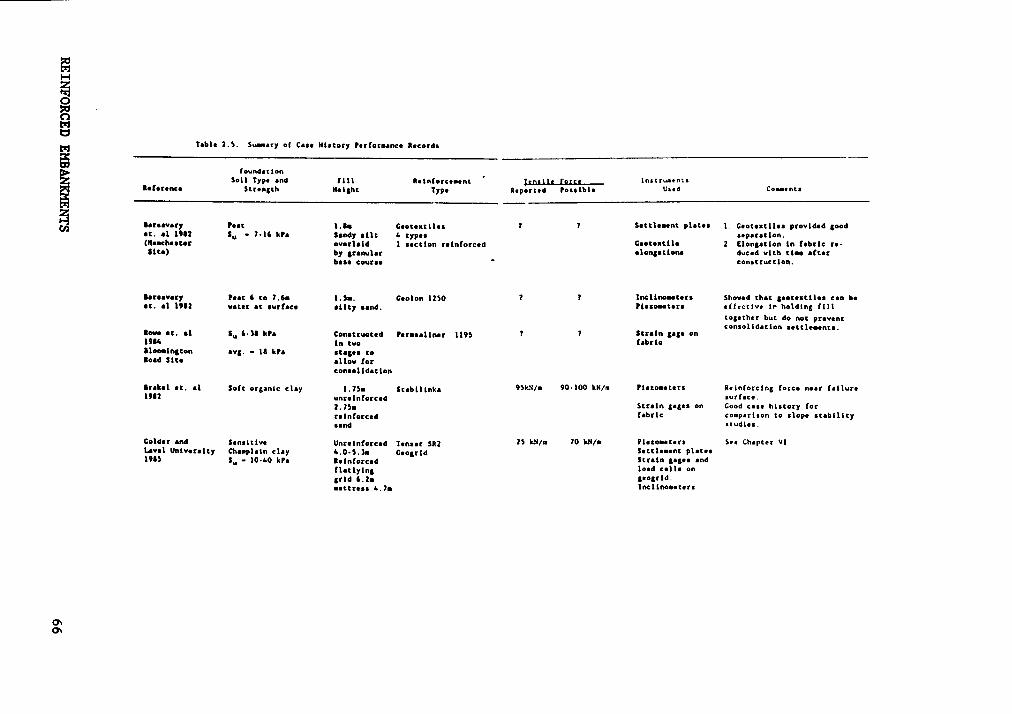
ÄZ
>•v
’S
0-
c“
:ä«
o•
Z.-E
Jq
IG
*—»
—>
léIn
Q••I
*3R
3•—
···;‘·
nä0
~'••"
“.,Ü
¤—•
ß'
""
:—
•••
••·
""2Z
•>·¤
„n
9V
_g
•••-•
6a
uß
IO
S-
¤U
_•·
9*·‘
¤Q
uu
>|
•c¤
.c—
-¤•
..0°
nn
hß
uh
l9
Ug
gu
gg
U•-D
•*c
cU
:::*3*:
2-"=
—··=·
zg
nn
vu
¤>
*"
:g§
:~:Ä
•U
IEIIanno:¤
•¤·¢
•'•U
6.,„,
U•«
-:0
•'~••'°
;•«¤
¤¤
Qn
uvu
!••=
a...;.¤
5:
•.
42
:oo
N5
00
!J;
,..gg
Illu
uü
Kllu
uu
·UII
:c
~¤
ug
II
UC
,.„Q
u••
I°
gnu
no
•«•
gll
•U
UQ
Q0
nQ
Il
_
Ug
99
üI
U¢
¤u
•¤
·:
=:2
23
-•··
··so
{:0
••
•=•I
"„
00
:•"
•a
n•u
s••0
2g_
0o
gg
gg
i..
0-
—-•_:_gg__
J.
6.
_—
wg
,A
.m
usu
{ggI
•-··
‘as
·>5
·•N
•-"
2o
26
"°
0LE
•{
..S·"
«•g
•„•~·
•*2
NI
E.2
~Q
S ·Ev•
9.
2:2
"R
E;
ggv
•-••·:
§S
„«:
vuhg
Cg
unU
0';
‘.U
gQ
••\g
~•
•I
U).
,.„5
nl
Ilg
IC
0•••·
2,
„••
•5
,,.,g
5.ve
O-0
E¢
I2
°*3
*3"
uu
0u
0I
~19
,.2,-gg
ue
n:
n•
n•¤
Q,
;q
Sn
aß
00
¤I=
__
_In
Qh
•••
|§
•In
§••*\
•O
gg
gM
Q!
••O
G0
C·£
:~G
~I-
·-'ßcu
vu
gg
gg
|•I
UG
OI
•I•f\C
UI•
g••G
gg
gg
9•~
••Q
I•°••l•
¤¤
•|
••0bg
2
2I>·•
UQ0
Q>
~I
":2
¤N
:,,
2:
>„o
•;
"‘vl:
••4
—·v
U••
an
·
QL
CO
Qu
uü
_Q
JG
IIC
QIB
C.
uuI
Gte
•«
IGC
F:
Qfl
I0
V.
2-n
v!
U.
9:
MQ
||
l~••
UQ
uG
§«C
I.
·•
,;
••
s>
¤•6
¤•^
*U
nQ
;vg
•0•
vlII
Q>~
··2:
I3E
1§
"'=2
°:•
·¤
>—
yä
ßIII
UG
d•
:*2
.„,.•
-Q
u•
•¤[
.•
gn
¤-•
_:
•>—
•&»~>
•;'
""”1
Ulf
°:„
•„•
ng-§
•¤•
••
•-·>•
‘:{g
gg
zu
••-••
n••
I1
•¤
•G
-G
•'*
bearing capacity failures took place in the fabric-reinforced sections.
Fabric strains of around 50 percent were measured after loading. The
depth of rockfill necessary to construct a useable haul road was the
serviceability criterion. On this basis, an unreinforced section re-
quired rock depths of five to eight feet while the reinforced sections
required three to six feet of fill.
2.4.3 Pinto Pass, Mobile, Alabama
An 800-ft-long sand embankment test section was constructed at Mobile,
Alabama, to verify that a geotextile could be used as a tensile re-
inforcement to construct an embankment over very· weak cohesive soil
(Haliburton et al. 1980). Subsurface conditions are shown in Figure 2.18
and consisted of very soft, highly plastic clays and loose clayey fine
sands and silts 40 feet thick overlying dense clean sands. The undrained
shear strength of the cohesive materials was 50 to 150 psf, with Standard
Penetration Test N-values of 0 to 5.
A sand fill embankment, 8 ft high, was constructed on a geotextile
fabric placed on the ground surface. The fill was a relatively clean,
poorly graded fine sand. The sequence of construction shown in Figure
2.19 was developed to balance forces on the soft foundation, and to pro-
vide proper anchorage of the fabric along the toes of the embankment prior
to placement of fill along the centerline. The embankment was constructed
with very gentle side slopes to allow the embankment to be raised gradu-
REINFORCED EMBANKMENTS 67
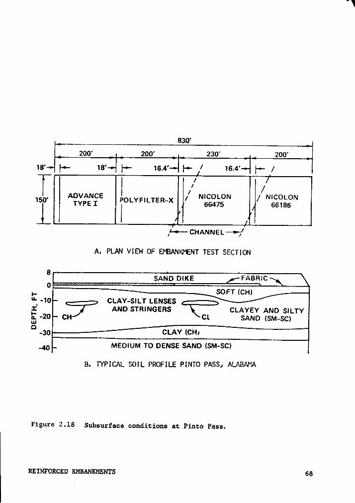
830'200' 200' 230' 200'
16* }-•— 16* |-— 16.4* I- / 16.4* I-- 1/I I / 1, -ADVANCE / NICOLON / NICOLONIT TYPE 1 VLYF'LTER"X 66475 66186
,1-- cHA~~E1.——;/
A. PLAN VIEW OF EMBANKMENT TEST SECTION
8 SAND DIKE FABRIC
I- .-10 CLAY-SILT LENSESI AND STRINGERS CLAYEY AND SILTY-20 CH CI. SAND (sm-sc)Q -3g CLAY (CH;
_40 MEDIUM TO DENSE SAND (SM-SC)
B. TYPICAL SOIL PROFILE PINTO PASS; ALABAMA
IFigure 2-18 Subsurface conditions at Pinto Pass.
REINFORCED EMBANKMENTS 68

ally over the next 20 years. Four geotextiles were used for the tensile
reinforcement along the locations shown in Figure 5.18.
Instrumentation consisted of five settlement plates and eight
Casagrande piezometers installed at each 100-ft station along the
embankment. The settlement plate risers were used to measure settlement
and horizontal displacement during and after construction.
The test section was finished to design width and height without
lateral splitting or rotational foundation bearing failure, despite ex-
cess pore pressures in the foundation soils rising six feet above the top
of the embankment. Based on measurements made on the settlement plate
risers, the lateral spreading of the embankment was minimal except near
the old channel. At this location, 3.8 ft of lateral spreading developed
over a width of 90 feet.
Settlements of about one foot were recorded during construction.
Consolidation settlements of one to two feet occurred during the first
six months after construction during which time the excess pore pressures
dissipated to less than 15 percent of their maximum values.
Based on the results of the field test program, Haliburton et al.
advanced the following conclusions:
1. Use of geotechnical fabrics to provide transverse tensile reinforce-
ment is a technically sound method of rapidly constructing
embankments on foundations too soft to support the unreinforced
embankment without failure.
REINFORCED EMBANKMENTS 69
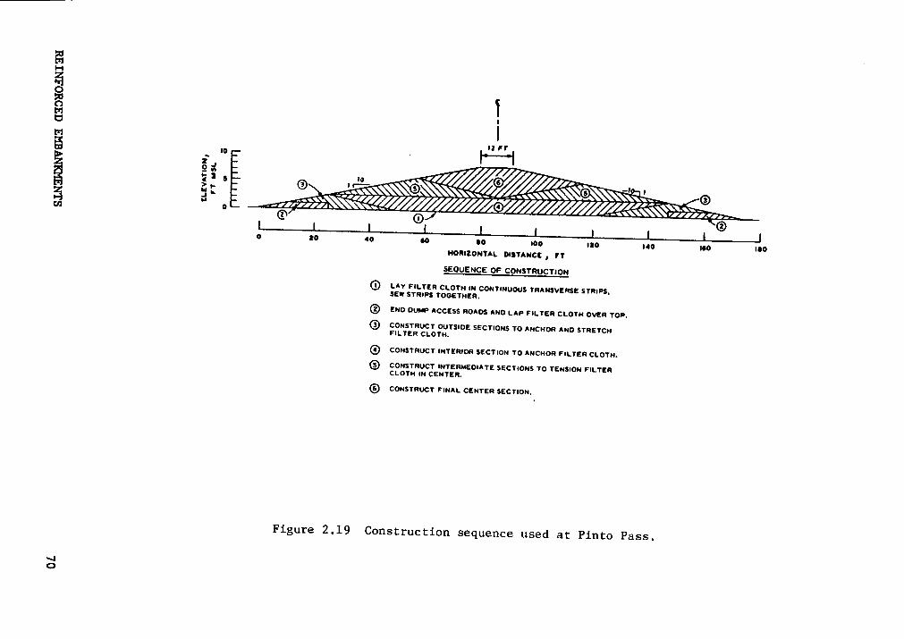
Ä2
Al
za?CU
ul
m
?¥
vi2
Eg
gÄ-F;
5sg
zuvr
QD
5;
·:2é
äe2
-zz.„
.—m
\‘j§
caäääääääE
.,@
@@
@@
@8
Ä'gg
°
N
Ä”
3ۤ
go
REINFORCEDEmsAN1<MEm's70
2. If procedures are used that provide essentially balanced loading on
the foundation and that cover the outside edges of the fabric to
suitable anchorage before placement of the interior embankment fill,
construction of fabric-reinforced embankments by using available
low-ground·pressure dozer equipment and conventional dump-truck ma-
terial hauling is operationally practical.
3. Compared with conventional end-dumping displacement methods, fabric-
reinforced embankment construction appears particularly cost effec-
tive. The additional construction costs of purchase and placement
of fabric are more than recovered by the savings of fill required to
construct the above-ground embankment cross-section.
4. Although specific situations will dictate exact fabric strength re-
quirement, high-tensile-strength, high-deformation-modulus fabrics
should prove to be the most suitable for embankment reinforcement.
5. There appears to be no particular advantage to constructing a working
table before fabric placement, as long as the ground surface is rea-
sonably level. When the mud-wave displacement method of fabric
stretching is used, the longitudinal seam strength should be equal
to or greater than the fill·direction tensile strength of the fabric.
Most importantly, this project demonstrated the feasibility of con-
structing geotextile-reinforced fills on weak soils and that tensile-
resistant reinforcement can benefit embankments built on weak soils.
}REINFORCED EMBANKMENTS7l
2.4.4 Almere, Netherlands
Two test embankments, one reinforced with a geotextile material and
the other an unreinforced control section, were constructed on a soft 3.0
to 3.5 meter thick clay deposit at Almere in the Netherlands (Brakel et
al. 1982). The tests were performed to assess the effect of geotextile
reinforcement on the stability of embankments on weak soils. The geometry
of the two sections is shown in Figure 2.20.
Brakel et al. (1982) described the soils at the site, the measured
results and visual observations of the field tests, and the results of
calculations on the stability of the embankments. The foundation soils
at the site consist of three to three and one-half meters of soft organic
clay overlying medium coarse, dense sand. The undrained shear strength
of the organic clay is about 8 to 10 kPa, based on cone penetration data.
To ensure that the embankments could be brought to failure, a ditch
was excavated in front of the embankments, as shown in Figure 2.20. The
excavated material was used to construct a retaining bank. Both the un-
reinforced section and reinforced section had a length of 60 m.
Stabilenka 200 polyester fabric was placed prior to construction of the
clay retaining bank and extended from the toe to this bank back 25 m with
an overlap of 30 cm. The fabric was instrumented with two rows of 10
strain gages placed transverse to the outer toe of the clay retaining
bank. Six piezometers were installed in each test embankment to monitor
pore pressures in the foundation.
REINFORCED EMBANKMENTS 72
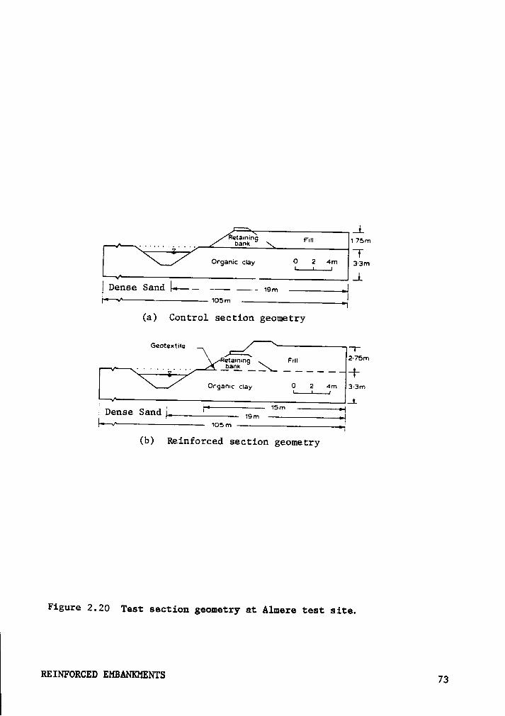
T .L
............ °°ää’iT"F' F"' "’F”“T
Organic clay O 24*** 3·3miii;
.L[ Dense Sand i•—— -— 19m}<—- iosm
(a) Control section geometry
Gcotoxtila T
‘ħ·?£"'L>_Ä'Ä--- +Organic clay O 2 4*** 3·3m
'i I-•— 15m
.•.|_L
i Dense Sand i,YÜÖFH(b)
Reinforced section geometry
Figure 2.20 Test section geometry at Almere test site.
REINFORCED EMBANKMENTS 73
Failure was induced by hydraulically filling sand behind the clay
retaining bank. Failure of the reinforced section occurred by circular
sliding at a fill height of 2.75 m. About one hour prior to the failure,
a one meter displacement of the fill towards the ditch occurred. The
measured reinforcement forces are shown for an instrumented section in
Figure 2.21. The maximum measured force was 95 kN/m with an average value
of about 80 kN/m at the time of failure. Excavation after failure re-
vealed that the fabric had ruptured, but that anchorage on either side
of the rupture location was sufficient. The unreinforced section failed
at a height of 1.75 m.
This field test shows the benefit of tensile reinforcement placed at
the embankment·fil1 interface simply on the basis of comparison of failure
heights of the two test sections. However, the real benefit of this case
history is in its use as a calibration tool for limit equilibrium proce-
dures. Brakel et al. (1982) performed circular arc calculations (assumed
to be the "Swedish circle" method) for an reinforced embankment height
of 3.5 m assuming tangential orientation of the reinforcement at failure
and obtained the results shown in Figure 2.22. Other limit equilibrium
analyses of this project have been carried out by Rowe and Soderman (1984)
and Low and Duncan (1985). In both of these studies an extended Bishop°s
Modified Method was used which allowed consideration of both horizontal
and tangential orientation of the reinforcement. Identical results were
obtained from these two studies as shown in Figure 2.22 and show excellent
agreement to the observed results. It can be seen that assuming
tangential and horizontal orientations results in calculated factors of
l
>REINFORCED EMBANKMENTS 74
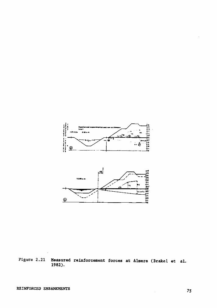
;é: . , .. ..„.‘$„—‘*° ”
ov! . •• V'- lwsz wg; 0gn" ‘—'=·=;„;é„-=—-» „»Q|· ‘ ‘ ·— _ '•••u Y
sé 3Sl-—
rw
-,VJ xr ~— ,‘§1¤.•¤•«•
I ../ N1 S
A °
,°‘§·„1 I2\__1
® =
Figure 2.21 Measured reiuforcemeut forces at Almere (Brakel et al.1982).
REINFORCED EMBANKMENTS V 75
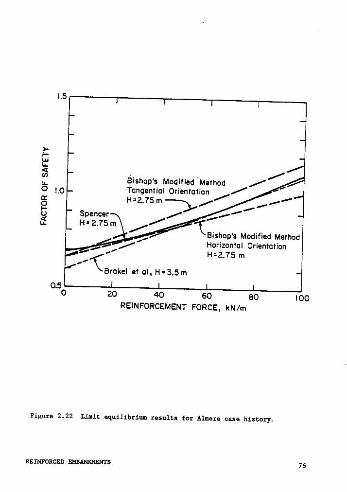
l.5
>-uilä
/Bishop‘s ModifiedMethod0LQ TangentialOrientationcz
i-i=2.vsm /,/’
E > ,/0 Spencer Z ,/E H=2.?5mBishop’s Modified Method
y' Horizontal Orientationm
(Brakel et al, H= 3.5 m0.5
0 20 40 60 80 IOORElNFORCEMENT FORCE, kN/m
Figure 2.22 Limit equilibrium results for Almera case history.
Rmuroucma Eimmomms 76
safety which form a band around the the true factor of safety of "l" at
failure. For comparison purposes, the factor of safety was also deter-
mined by using Spencer°s method (Spencer, 1968), extended to account for
reinforcing in the manner outlined in Section 2.2.3. These results are
also shown in Figure 2.22. It can also be seen that using Spencer°s
procedure with horizontal orientation of the reinforcement yields results
in near perfect agreement with the measured results. These results are
nearly half-way between the BMM results shown. The results of these limit
equilibrium analyses are encouraging when consideration is given to the
accuracy with which the in situ shear strength of soft clay can be meas-
ured.
2.4.5 Bloomington Road, Ottawa, Canada
Rowe et al. (1984) described the design, instrumentation and field
performance of a 1 to 1.5 meter high geotextile·reinforced embankment
constructed on peat. The site was designated as Bloomington Road and is
located near Aurora, Ontario, Canada. Foundation conditions at the siteare shown in Figure 2.23. It can be seen that the depth of the peat de-
posits varies considerably along the centerline. The upper one meter of
the peat deposit was classified as amorphous, containing wood, fine fibers
held in a woody, coarse, fibrous framework while the the underlying peat
was a nonwoody, fine, fibrous peat. The peat was underlain by silty sand
and sand.
} REINFORCED EMBANKMENTS 77
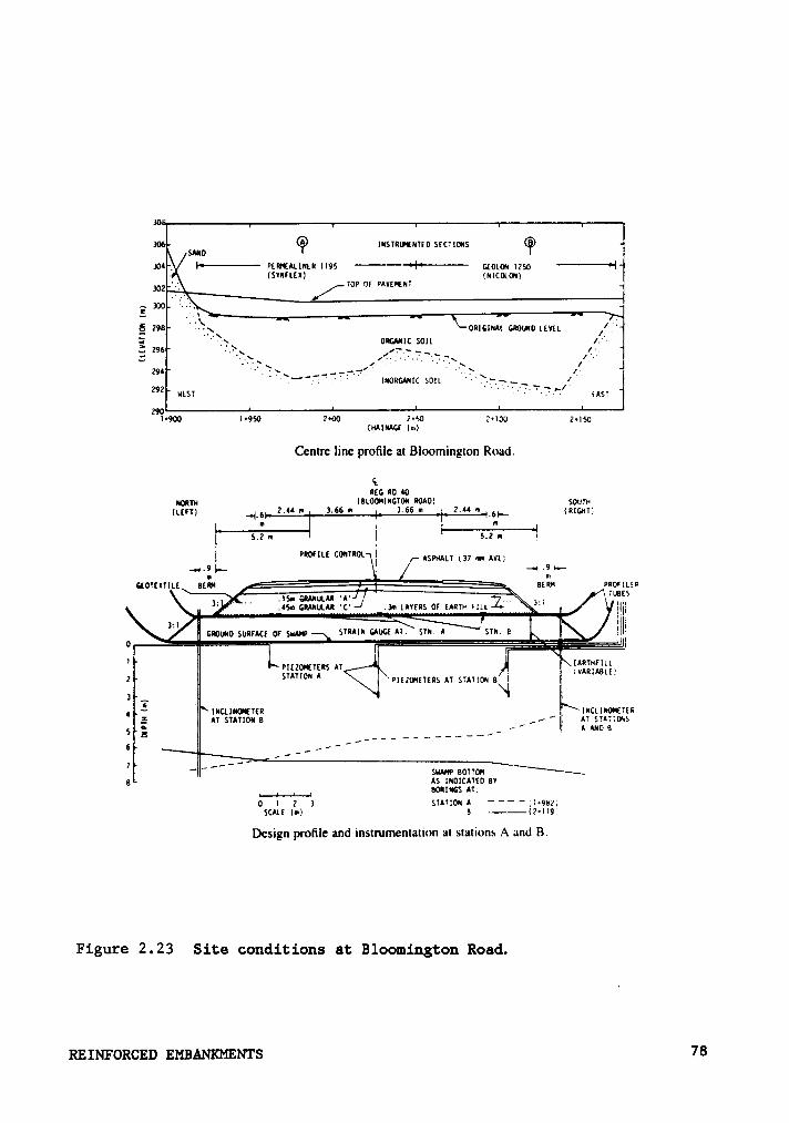
30•· INSTRIHNTED SFCTTUIS G) 1SMDDA ll95 GLOLON
IZSO(SVNFLUI(NlCOI.0N)mz TOP OF PAVUINT2
’°°dr:.
298 0RlGlNAl cmuno tcvu. //„C'
= ORGANICSOILZ296 4-.
~1‘294I ”‘.*$¤ ,-•-r’-<Ä- Ä J‘ ·T—·f_7’.
·¤* " 1«ouc1•11c son ‘·‘Ä.:—A-_ _ /4‘
292 utsr H (16:290l•900 l•950 2•00 2•bO 2~I00 2•l5G
CNAINAGI fm)
Centre line profile at Bloomington Road.
G.REG RO *0
ygggm (BLOGHNGTON NAD) SOUTH(Lgn) -4.6 2.44 Il 3.66 ll 1.66 ll 2.** M -6•__
(RIQMT}gg * n1
5.2 m I 5.2 111 4”°"'·E C°""‘°‘·
I ASPNALT (:7 mn 1vz:.,1 .9 _ —•• .9 I•—
*1*J'ÄGIANULAI 'C' .3n LAVERS OF EARTHFILL::1
' V I 'III’ AI GFDWO SURFAC! OF SHARP STRAIN UW! ATI STN. A STN.E‘l‘
EARTHFILLPIEZOKTERS AT (VARMBLE-.1 SI^"°" ^ ‘Pl£l(!\£TERS AT STATION s I 1*~ I \‘R‘ 5 Ä
INCLINGKTER INClI*Ü*ÜÜE AT STATION B ,«
’AT SYATIMS
5 g f « ’ 1 AND G6 _ „
-’ l a ’— H - -
7 , „· * ’_ ß
‘$111MvBono!gAS INOICATEO BVBOHINGS AT;
0 I 2 1 STATIONA "" "(I•9Bl}SCALE (111) B -—l(2•\l9
Design profile and insu*umenta1ion at stations A and B.
Figure 2 . 23 Site conditions at Bloomington Road.
REINFORCED EMBANKMENTS 78
A geotextile-reinforced embankment was selected after conventional
construction methods were rejected due to either cost or construction
difficulty. The geotextile was selected primarily on the basis of a
circular arc stability analysis and the following assumptions: (a) The
geotextile was placed with the stronger direction transverse to the fill
alignment, (b) The tensile forces required to maintain stability can be
mobilized at relatively small strains and (c) The tensile force in the
fabric will act tangentially to the failure arc. To increase the factor
of safety to 1.3, tensile forces of 20 and 39 kN/m were calculated to be
needed at Stations A and B, respectively. The requirement that the sta-
bilizing force be developed at relatively small strains implied that the
geotextile reinforcement should have a high strength under relatively
small elongation and this governed the selection of the geotextiles used.
At Station A, a calandered polypropylene monofilament with plane weave
was used. At Station B, a plane weave, twisted, polyethylene, slit film
was used. Based on stability calculations, the force required to maintain
a factor of safety of 1.3 against rotational failure represented approx-
imately 0.5 and 0.3 of the estimated ultimate strength of the geotextiles
at Stations A and B, respectively.
Instrumentation consisted of piezometers, hydraulic and electric
gages to measure fabric elongation, inclinometers and settlement plates.
The location of some of the instrumentation is shown in Figure 2.23.
Construction took place in stages. Due to swampy conditions at the
site, a working platform varying in thickness from 0.3 to 1.0 m was con-
structed prior to placement of the geotextile. Lift thicknesses of 0.3
REINFORCED EMBANKMENTS 79
m were used with the geotextile folded back three meters over the first
lift to provide anchorage. The outside-inside construction sequence ad-
vocated by Haliburton was used.
During stage I construction, 1.37 m of fill was added at the
centerline. Immediate settlements were about 50 percent of the total
height of fill added and settlements increased to 75 percent of original
fill height prior to stage II construction. Dissipation of excess pore
pressure occurred within 60 days of construction.
The progress of settlement with fill height at Stations A and B is
shown in Figures 2.24 and 2.25. Significant immediate settlements oc-
curred (50 percent of original fill height at Station A and 90 percent
of original fill height at Station B) with stage I loading. Consolidation
settlements prior to stage II increased the settlement to 95 percent of
original fill height at Station A and at Station B the fill became almost
completely submerged.
Stage II construction resulted in significant additional settlement
at both stations. At Station A 2.5 m of additional fill yielded on 0.8
m of net fill height at the end of six months of consolidation following
construction. Geotextile strains as high as 21 percent were measured in
the transverse direction and eight percent parallel to the axis.
Most of the settlement during stage I was attributed to compression
of the underlying peat and the geotextile had negligible effect. However,
lateral movements and "mud waves" observed during stage II suggested that
a large component of stage II settlement was due to shear deformation
which resulted in the development of significant fabric strains.
, REINFORCED EMBANKMENTS 80
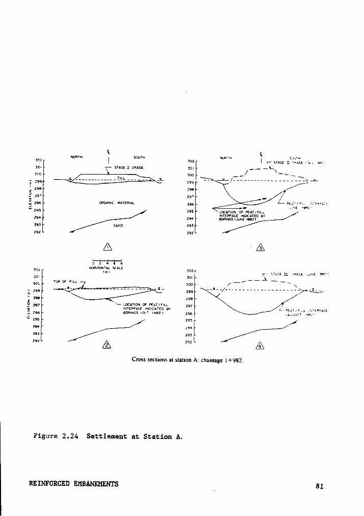
Q Q INonne soune Nonne 6.··„v•-SQ2 I 302 I <— smc: IZ nnut ·~t» SBE:0. ·-— smc: 1 cmxo: 30: .. - — \—\:00 soo ,..-1_y_
- - ..7.. /-...---..- ---..---.-k_L
299 299 · —; zsa 298O /
E297 297
29; cncnmc Mnrcmnt 296pw pm: ¤9¤2>295 295 LOCATION OF P:Ar1r•tt
tNYERFAC£ •~o¤cAY:¤ av294 294 Boütucs t.:u~E •962t293 sum 293292 292
0 2 4 6 6nomzoumt scnt:mz Im) mz «—— smc: z30• ·_
—-worover rrtt wo
-1- ·--!-- --..-........—„------- -¤--9 299 299 / >—
296 296zQ 297
‘¤tO(AT•ON OF PELT/Fett 297 1; ¤~TE¤FAC: ¤ND¤CATED BV
gg; BOR•~cS t0CT ¤982>296‘“266 296294 29629: 266292
2292
C
Cross sections at station A: chainage l+982.
Iw
I
Figure 2.24 Settlement at Station A.
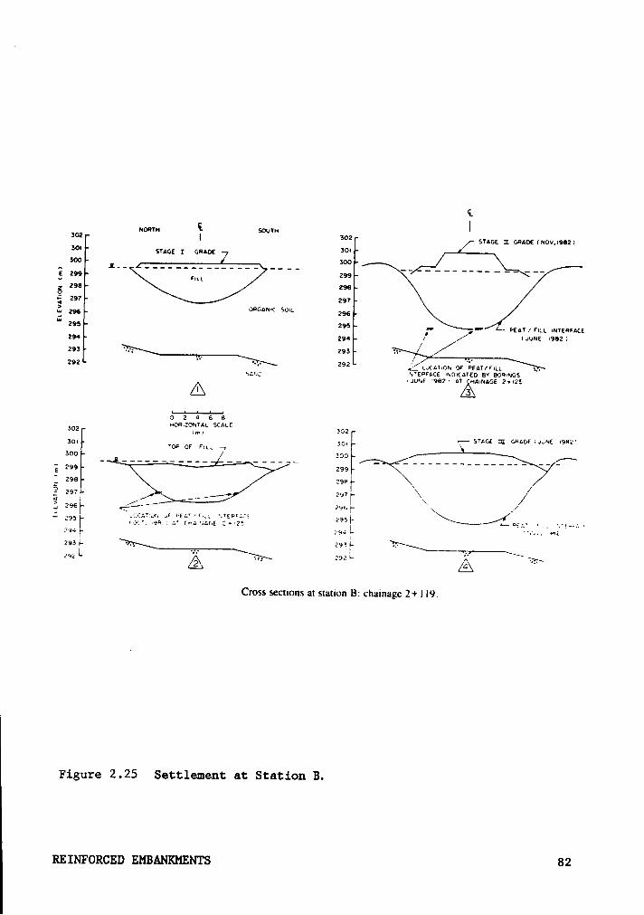
Quomu Q soum I3°2 I 9°2 /— suse ZI same ¢~ov.¤9s2>‘°'
suse z snuoe ’°'soo 100.. J--- --------------- -•-• -2 -..-- ..__________
E 299 ml 299S 296 298E 297 297> oesnmc seinE 296 296295 295 ;• PEAT 1 f•;|_ •NT£RFACEggg ggg / ( JUNE l982 )
293 293 tz-292 °"' 292 •.J<At¤o« or 'i>eAr/mr g,.
5,m;, INTEPFACE ¤~0¤cAY€0 8* 80¤¤~6S~.¤uNE i962) AT r1A¤NAGE 2•¤25Ä Ä
0 2 ¤ 6 6mz ·—— suse HI cause uwe •962·or FiLL .., am 2,
soo ' :00 /„Q 299 299v 29829nZ2 292 ·»97 \
·/~„ 2 }" \ /3 296}- é,-···‘
296 }-X\ //
.1 „ ‘2;;::;:6: c wer! » =.„ ~.ve¤r;r; . __
k32}* (on', 2. ‘-'P-‘-'-·1*94}- 29.: L •¤2293 L 7~·\·._
29:}-292L
C2,, 292*—4
Cross sections at station B: chainagc 2+ l I9.
}
Figure 2 .25 Settlement at Station B.
Stage III construction consisted of removing fill, placement of an
asphalt road surface and shaping of the shoulders and side slopes. Ad-
ditional settlements of 0.1 and 0.2 m were measured stations A and B in
the months following construction. Following completion of the road,
differential settlements in the transverse direction were minor while
significant differential settlement occurred in the longitudinal direc-
tion.
Based on the observed performance of these geotextile reinforced fills
Rowe et al made the following observations:
1. Large settlements were observed at both instrumented sections with a
maximum fill thickness of 5.7m resulting in a corresponding settle-
ment of 4.7m.
2. Large lateral movements on the order of one to two meters occurred.
3. The geotextile at the edge of the embankment appeared to be unstressed
and hence folding back of the fabric was unnecessary.
4. When settlement was due primarily to compression of the peat,
geotextile strains were small despite large settlements.
5. When large shear deformations were apparent, large fabric strains and
forces developed.
6. Longitudinal strains in the fabric were significant.
RE1NF0RcED EMBAN1<r·mN'rs 83
7. The field data make it apparent that the use of a single layer of a
very strong geotextile did not prevent large shear deformations.
8. In light of the performance of this embankment, simplified limit
equilibrium procedures should be viewed with considerable caution
when designing geotextile-reinforced embankments on peat.
2.5 Summary and Conclusions
Based on the above discussions the following conclusions can be drawn
concerning the behavior of reinforced embankments over weak soils.
l. The use of Bishop's Modified Method, extended to include horizontal
reinforcement forces, provides a reliable, slightly conservative
procedure for evaluating the factor of safety of reinforced
embankments.
2. The factor of safety calculated assuming the reinforcement becomes
aligned tangent to the slip surface at failure is considerably higher
than that calculated assuming the reinforcement remains horizontal.
3. Based on the analysis of the Almere Test embankment, the actual factor
of safety is likely to be approximately equal to the value computed
using Spencer's procedure with horizontal reinforcement, and about
halfway between values calculated using Bishop°s Modified Method us-
ing horizontal and tangential orientation of the reinforcement.
iREINFORCED EMBANKMENTS 84

4. The optimum location for placement of the reinforcement is at the
embankment-foundation interface.
5. Reinforcement has very little effect on consolidation settlements,
but it does tend to reduce differential settlements at the top of the
embankment.
6. The major effect of reinforcement is to reduce lateral spreading and
to increase stability. This is accomplished by reducing shear
stresses and plastic flow in the soil through an increase in con-
finement pressure in the embankment and foundation soils.
7. At low load levels (where the factor of safety is high), reinforcement
does not significantly impact embankment behavior.
iREINFORCED EMBANKMENTS 85

·CHAPTER III
PROCEDURES FOR FINITE ELEMENT ANALYSIS
3.1 Introduction
The review in Chapter II showed the feasibility of using finite ele-
ment analysis procedures for the analysis of reinforced earth structures.
This chapter describes the finite element techniques used in this dis-
sertation for the analysis reinforced soil structures, particularly re-
inforced embankments and foundations. The method used employs an
elasto-plastic stress-strain soil model and allows consolidation effects
to be modelled directly. Reinforcement is modelled using bar and membrane
elements.
The program used in the analyses in this dissertation was originally
developed by Chang and Duncan (1977). The program, called CON2D, was
developed to model consolidation behavior of partially saturated soils.
During its development the original Cambridge Cam Clay model was extended
to provide for more suitable representation of the strength and stress-
strain behavior of compacted clay. Further improvements to the program
were made by Duncan et al. (1981). An axisymetric version of the program
was developed by D°0razio and Duncan (1982).
This chapter will review the formulation of the soil model - the Cam
Clay model, the formulation of the finite element equations, and the ex-
tensions made to the program. The program has been adapted to the
PROCEDURES FOR FINITE ELEMENT ANALYSIS 86
l

Virginia Tech IBM system, has been extensively rewritten to adopt the
efficiencies of structured programming and to document the algorithms of
the program, to extend the program to handle static pore water pressures,
and to incorporate finite elements for the modelling of reinforcement.
With these changes, the program was renamed CONZD86.
3.2 Soll Model
3.2.1 Cam Clay Model
Drucker, Gibson and Henkel (1957) were the first to suggest that soilcan be modelled as an e1asto—plastic material with work hardening or work
softening effects. Based on these ideas and the concept of critical void
ratio (Casagrande 1936), Roscoe, Schofield and Wroth (1958) developed an
isotropic, strain-hardening model to predict the stress-strain behavior
of remolded clays. Subsequent modifications by Roscoe and Schofield
(1963), Roscoe, Schofield and Thurairajah (1963), Burland (1967) and
Roscoe and Burland (1968) resulted in the model known today as the Modi-
fied Cam Clay Model.
The soil model used in CON2D86 is an extended version of the Modified
Cam Clay Model. The sections below describe the model as it is imple-
mented in CON2D86 and CONSAX86. Discussions of the original Cambridge
_ version can be found in Schofield and Wroth (1968) and Atkinson and
Bransby (1978).
PROCEDURES FOR FINITE ELEMENT ANALYSIS 87
The Cam Clay Model was developed for triaxial conditions and was
subsequently extended to general states of stress. The relationships are
formulated in terms of the stress invariants p’(the mean normal effective
stress) and q (a generalized deviator stress). In terms of the stresses
referred to an x, y, z coordinate system, p' and q can be expressed as
follows:
p' = + oa, + o'z) [3.1]
6 = @[16,, -6,32 + 16,, - 6,>2 + 16, — 6,)*2 + 66,Ey] 13.21
An elasto—plastic model requires definition of a failure surface, a
yield surface to differentiate elastic and plastic behavior, and a flow
rule and hardening rule which relate plastic strain behavior to stress
changes. These are described in the following paragraphs.
Egi1g;g_§g;fggg„ In the Cambridge version, the failure surface for
the Cam Clay model was a straight line through the origin. To represent
soils which have a cohesion intercept, the failure surface was revised
by Chang and Duncan (1977) as shown in Figure 3.1a, and is represented
by the equation
<1j= MW + pr) [3.31
in which qf== value of q at failure, or shear strength, M = strength pa-
rameter, and pr = an intercept stress.
Additionally, the failure surface was modified to reflect the behavior
of soils which exhibit a curved failure line, Figure 3.lb and those which
PROCEDURES FOR FINITE ELEMENT ANALYSIS 88
possess tensile strength, Figure 3.1c. Figure 3.ld shows the complete
failure surface in q—p’
space.
XiglQ_§g;jggg„ The yield surface in the Cambridge model is assumed
to have an elliptical shape as shown in Figure 3.2. The surface is de-
fined by the equation
2(1 + + pr) —
Pr = py, [3-41M
where q =-7-E--· and pb is a preconsolidation pressure.(p + pr)E1gw_Rglg„ The flow rule relates the plastic strain increments to
the existing stress state. The plastic strain increments are assumed to
occur as outward normals from the yield surface, as shown in Figure 3.2.
For such conditions, the plastic potential function and the yield surface
are identical and the flow rule is termed associated. The extended ver-
sion is the same as the original version in this respect.
Hg;gggigg_jgg„ The hardening parameter describes the magnitude of
the plastic strain increments. The slope of the ellipse at the stress
point determines the relative magnitude of the plastic strain increment.
As shown in Figure 3.2, the plastic strain increment can be divided into
a plastic volumetric strain aß and a plastic distortional strain gg (or
shear strain). Thus the magnitudes of all the components of the plastic
strain can be related to the value of the plastic volume strain.aß which
can be calculated by
aß = 0. — x)in-% [3.4]P
PROCEDURES FOR FINITE ELEMNT ANALYSIS 89
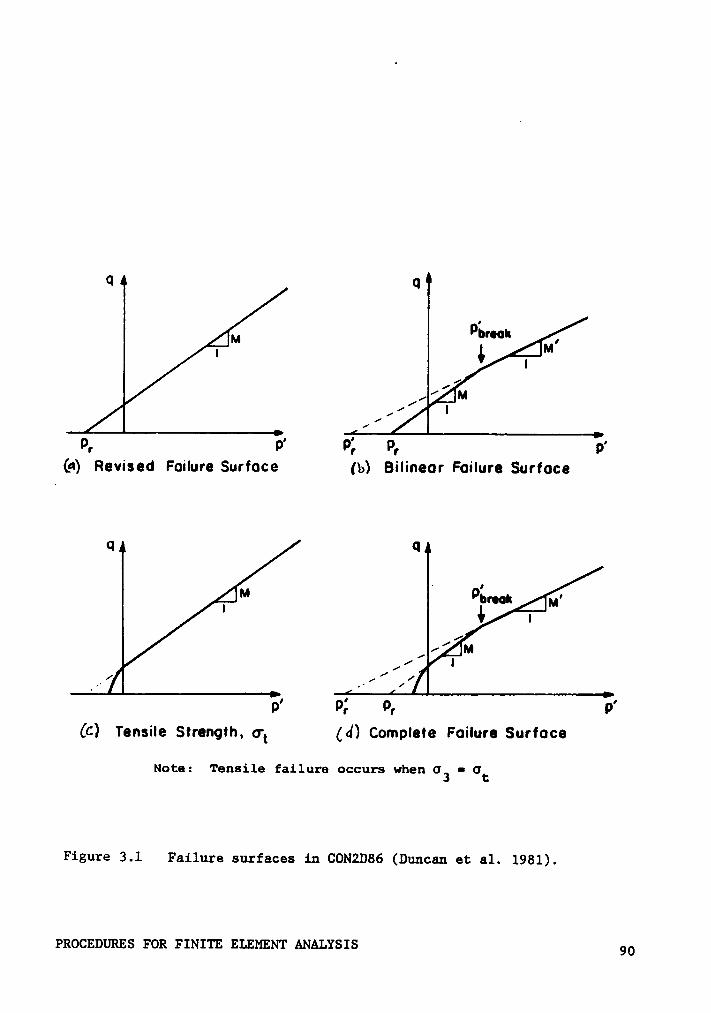
9 G
M pßrtck M,l { I
//"x l
o, p' ¤; P, p'(A) Revised Failure Surface (b) Bilinear Failure Surface
Q Q
‘I
IM ppm: M'
Ö •
//, / M
/•
.’ .// ,’
o' Pi P, P'(c) Tensile Strength, 0*, (4) Complete Failure Surface
Note: Tensile failure occurs when 03 • Gt
Figure 3.l Failure surfaces in CON2D86 (Duncan et al. 1981).
PROCEDURES Fox F1N1'1'E ELEMENT ANALYSIS 90
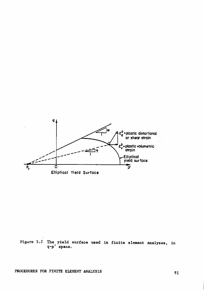
Q_9 · · ·| Ed =plast¤c dastorfionalor shear stroin
· 85 • Dlasfic volumefric/ sfrainz»,,’
Ellipiical,:„„·' yield surface
nr 0 ¤'Elliptical Yield Surface
Figure 3.2 The yield surface used in finite element analyses, inq-p' space.
PROCEDURES FOR FINITE ELEMENT ANALYSIS Q1
where A and x are the slopes of the virgin and rebound compression curves,
as shown in Figure 3.3, and Pb is the preconsolidation pressure.
Elg;;jg_ßghgyig;* At stress states inside of the yield surface, only
elastic strain increments result from stress increments. All of the
components of elastic strain are related to the stress increments through
the Generalized Hooke's Law. Any two of the elastic parameters E, Young's
Modulus; v, Poisson's ratio; G, shear modulus; or B, bulk modulus, can
be specified to determine the magnitude of the elastic strains. In
CON2D86, the parameters used are Poisson's ratio and the bulk modulus.
The bulk modulus is calculated from
6 = ii"+ Ö",[3.6}x
This provides for nonlinear stress-strain behavior because B varies with
the mean pressure, p'.
3.2.2 Material Parameters
The material properties that describe a soil model should be easily
determined from conventional laboratory or field tests. The Cam Clay
model described above can be defined by the following six parameters.
pr an intercept stress to represent a cohesion intercept;
Al the slope of the failure line in q-p' space;
x the slope of the rebound rebound consolidation curve;
A the slope of the virgin isotropic consolidation curve;
v Poisson's ratio;
PROCEDURES FOR FINITE ELEMENT ANALYSIS 92
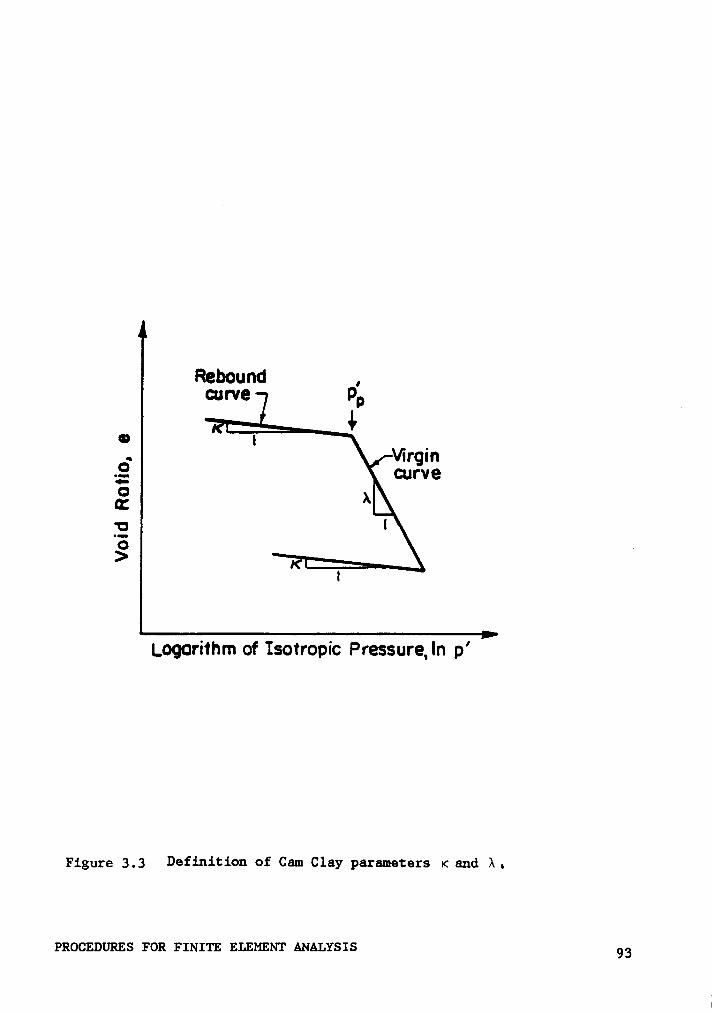
Rebound ,ourve Pp
na 4 _. Wrgm
.2 curveEpg >„
5 IQ .
>4
Logorithm of Isotropic Pressure, In p'
Figure 3,3 Definition of Cam Clay parameters 4< and A .
pxoczmuxzs von Fxuxm E1.mmm· Amusxs 93

60 the initial void ratio.
A , x and eo can be obtained from an isotropic consolidation test as shown
in Figure 3.3. The intercept stress, pr, and the slope of the failure
line, M, can be determined using the effective strength soil parameters
V and d in the following equations.
pr = c'cot V [3.6]
and
M = [3:7]3 ·— sm V
The value of Poisson's ratio may be determined from triaxial compression
tests using the procedures outlined by D'Orazio and Duncan (1982). In
CON2D86, the value of Poisson's ratio may vary with p’the effective mean
noraml pressure.
3.2.3 Undrained Sheer Strength
One of the applications of the Cam Clay Model is the prediction of
the undrained shear strength of a clay because the undrained shear
strength depends on the effective strength of the clay. Relationships
for the variation of undrained strength Su with effective consolidation
pressure can be derived in terms of the Cam Clay parameters. One such
relationship was presented by Poulos (1986):
PROCEDURES FOR FINITE ELEMENT ANALYSIS 94
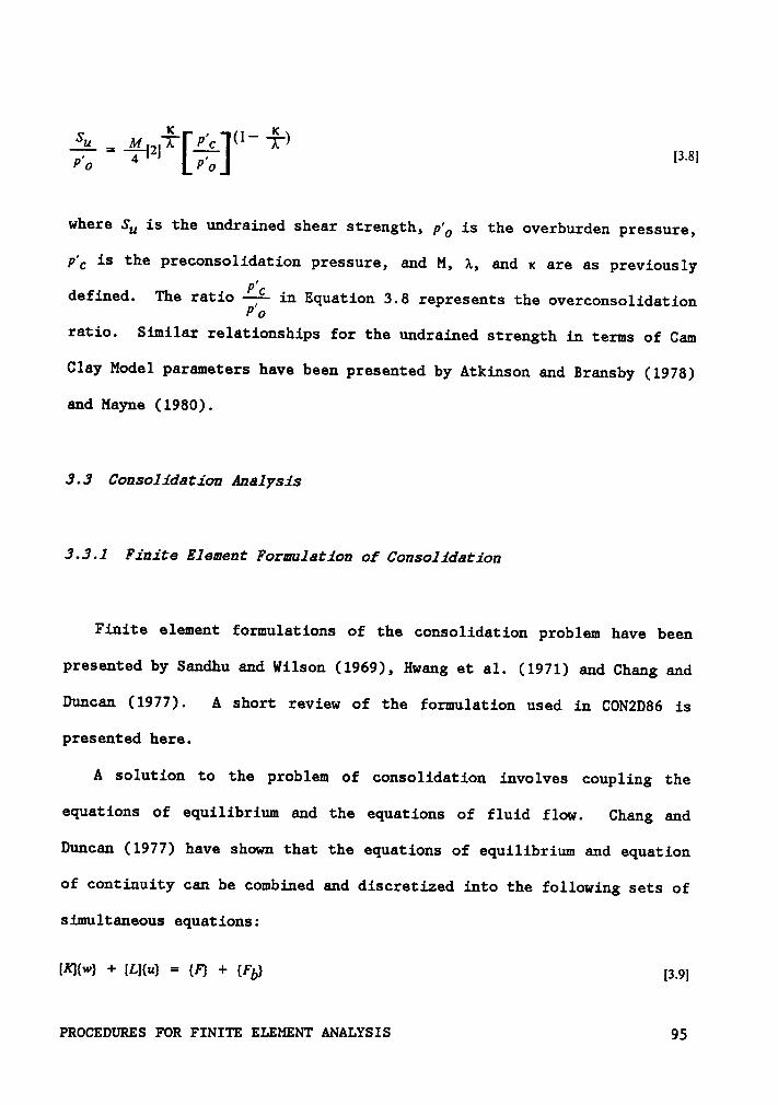
S p'= %l2| {3.81Po Fo
where Sk is the undrained shear strength, pk is the overburden pressure,
pk is the preconsolidation pressure, and M, 1, and x are as previously
defined. The ratio läi in Equation 3.8 represents the overconsolidationFo
ratio. Similar relationships for the undrained strength in terms of Cam
Clay Model parameters have been presented by Atkinson and Bransby (1978)
and Mayne (1980).
3.3 Consolidation Analysis
3.3.1 Finite Element Formulation of Consolidation
Finite element formulations of the consolidation problem have been
presented by Sandhu and Wilson (1969), Hwang et al. (1971) and Chang and
Duncan (1977). A short review of the formulation used in CON2D86 is
presented here.
A solution to the problem of consolidation involves coupling the
equations of equilibrium and the equations of fluid flow. Chang and
Duncan (1977) have shown that the equations of equilibrium and equation
of continuity can be combined and discretized into the following sets of
simultaneous equations:
[KI{w} + ILl{¤} = {F} + {Fb} [2.9}
PROCEDURES FOR FINITE ELEMENT ANALYSIS 95
Y
and
"{H]{¤} + lG}%{w} — [F}j,!T{¤} = {V} [3~l0]
In these equations [w} and {u} are the nodal displacements and pore
pressure, respectively. The integral definitions of the matrices and
vectors may be found in Chang and Duncan (1977), and similar sets of
equations were described by Christian (1977) and Hwang et al. (1971).
The physical significance of the matrices and vectors are:
[K] soil stiffness matrix
[G]=[LJT coupling matrices between the stiffness and fluid flow equations
[H] transmissibility matrix
[E] fluid compressibility matrix
{F} vector of nodal loads
{Fb} vector of body forces
U3 vector of specified fluid velocities on boundary surface.
Included in Equation 3.10 are terms relating to the flow of fluid in
soil ([H]) and the compressibility of unsaturated soils ([E]). The ad-
ditional soil parameters required to describe the consolidation and un-
saturated behavior of the soil include the unit weight of water, the
vertical and horizontal permeability of the soil, and the degree of sat-
uration.
Because Equation 3.10 contains derivatives with respect to time, in-
tegration over time is necessary to obtain solutions. In CON2D86, a fi-
nite difference solution to the time integration is used, with a fully
PROCEDURES FOR FINITE ELEMENT ANALYSIS 96

explicit method specified. Combining the time integration with Equations
3.9 and 3.10 provides the matrix equation:
[K] [L] w F + Fb
[ T H] tl = :1 + [3.11][L] — [H]9A: — [ u 9AzI‘
0
{(1·9)A¢{1'};0 + (IHl(1—6)A¢ ‘ [E]){¤}go + [l·]T(W}gO}
where 9 is a time parameter. If the solution is known at :0, then it can
be found at rl , and hence at rn by forward marching.
In the original derivation of Equations 3.9 and 3. 10, Chang and Duncan
(1977) formulated the pore pressures in terms of excess pore pressures.
At the suggestion of Chen (1984), the present version of the program has
adopted the total pore pressure approach wherein static pore pressures
b are taken into account.
3.3.2 Stability Gritarion
The stability of consolidation analyses has received considerable
attention by investigators and many interpolation schemes have been pro-
posed for the time domain. Booker and Small (1975) showed that uncondi-
tionally stable solutions result if 9 in Equations 3.7 and 3.8 is greater
thanä
. Despite this, finite element solutions of consolidation often
exhibit oscillatory pore pressures (Sandhu et al. 1977 and Read 1984).
Vermeer and Verruijt (1981) investigated the oscillation phenomena and
PROCEDURES FOR FINITE ELEMENT ANALYSIS 97
concluded that a lower limit on the time step, based on the coefficient
of consolidation and the mesh size, could reduce the occurrence of
2oscillatory results. The limit proposed was Az 2 %Ti%é%— where Ah is the
mesh size adjacent to the draining boundary, 9 is the time integration
parameter and c is the coefficient of consolidation. This limit on the
size of the time steps is recommended when using CON2D86.
3.4 Finite Elements Used in Program
3.4.1 Soil Elements
Isoparametric elements having a variable four to eight node config-
uration are used to represent the soil. These elements were developed
by Bathe and Wilson (1973). These elements allow considerable flexibility
in mesh layout for complicated geometries. In general, eight node ele-
ments are used where pore pressure degrees of freedom are required and
four node elements where they are not. Triangular elements can be formed
by superimposing nodes.
3.4.2 Reinforcing Elements
The representation of reinforcement was incorporated into CON2D86 as
a simple, two-node bar element capable of sustaining axial tension or
compression and having no flexural stiffness. The element equations for
PROCEDURES FOR FINITE ELEMENT ANALYSIS 98
such an element can be found in several standard finite element textbooks,
such as Reddy (1984), and Weaver and Johnston (1984).
Analyses of reinforced foundations for three-dimensional conditions
were simulated using axisymmetric analyses with the program CONSAX86 and
an axisymmetric membrane element. The element is capable of transmitting
radial tension or compression, but provides no flexural stiffness. The
derivation of the stiffness matrix for this element is given in Appendix
B.
3.5 Extensions to the Program
The incorporation of reinforcing elements and the provision for han-
dling static pore water pressures have been discussed in previous
sections. The most important modification to the program involved re-
writing the code to adopt the efficiencies of structured programming.
Structured programming is a philosophy of programing that focuses
on the importance of structure for the intellectual manageability and
reliability of programs (Kernighan and Plauger 1974). The main concerns
are the reduction of program complexity and program correctness. It was
with these goals in mind that CON2D86 and CONSAX86 were extensively re-
written using structured programming. The resulting code is more effi-
cient because dead code has been removed, and is easier to follow and
understand. Many of the algorithms used to in the program are documented
in the source code. This is of particular importance in program codes
which are in the research realm, and are continually being modified.
PROCEDURES FOR FINITE ELEMENT ANALYSIS 99
Additional, more detailed documentation and a user's guide are pro-
vided in Appendices C and D.
PROCEDURES FOR FINITE ELEMENT ANALYSIS 100
CHAPTER IV
REINFORCED FOUNDATIONS
4.1 Introduction
A reinforced foundation is a soil foundation containing tension-
resistent inclusions that increase the ultimate bearing capacity of the
system. Reinforced foundations are distinguished from reinforced
embankments by the fact that they are level areas designed to support
external loads in addition to the weight of the soil. Two types of re-
inforced foundations are shown in Figure 4.1a: one involves reinforcement
of cohesionless soil, and the other involves reinforcement of
cohesionless soil overlying weak cohesive soil. The latter condition is
the focus of the present study.
A problem of practical interest requiring use of reinforced founda-
tions arises in the construction of oil field drilling pads in areas where
soft clay and peat make up the foundation soils. The plan area of these
pads is about 100 meters square, and loads from various sources such as
hauling equipment, storage tanks, and drilling equipment exert beering
pressures of 15 to 150 kPa (300 to 3000 psf) on the surface (Kroshus and
Varcoe 1984). Additionally, peak loads applied to the foundation by a
crane raising the drill stem can be es high as 1000 kPa (21,000 psf).
With undrained shear strengths in the range of 5 to 20 kPa (100 to 400
psf), these loads cannot be supported by the foundation soils without use
REINFORCED FOUNDATIONS 101
1

Cl O
Reinforcing gSoft Clay'_Sand
(al
Sand or Q Q QGravel
lClayor Feat Su = 5 to 20 kFa= l0O to 400 psf
(bl
Figure 4.1 Reinforced foundations.
i
REINFORCED FOUNDATIONS 102
of a very thick pad or a reinforced pad. At present working pads are
constructed from local source materials or select fill to spread the loads
out over larger areas. In areas where suitable fill materials are not
available such material must be imported, often from large distances.
The use of reinforcement can reduce the quantity of fill needed. thereby
reducing costs. The magnitude of settlement is relatively unimportant
in these projects, so long as differential settlement is minimized and
bearing failure does not occur. Examples of the conditions that must be
considered are shown in Figure 4.1b. The imposed loads may be resisted
by one or more layers of a reinforcing material. At present no rational
procedures exist by which the amount of reinforcing needed can be deter-
mined.
This chapter will review previous studies of bearing capacity of sand
overlying soft soils for both unreinforced and reinforced conditions.
An approach for the determination of the bearing capacity of reinforced
soil over soft soils is presented and compared to the results of model
test studies. The results of a finite element analyses of reinforced
foundations are also presented and discussed.
4.2 Previous Work on Bearing Capacity of Sand Overlying Soft Soils
4.2.1 Model Tests
Binquet and Lee (1975) were the first to show that reinforced soil
technology could be applied to increase the bearing capacity of sand.
REINFORCED FOUNDATIONS 103
In a landmark series of laboratory model tests they showed that horizontal
reinforcing strips could increase bearing capacities up to four times
those of similar unreinforced granular foundations.
Binquet and Lee identified three mechanisms by which bearing capacity
failure could occur: shear failure of the soil above the reinforcement,
pullout of the reinforcement from the soil, and breakage of the re-
inforcement. These modes of failure are illustrated in Figure 4.2. It
may be seen in Figure 4.2c that discontinuities of the reinforcement are
shown near the edge of the footing. Binquet and Lee noted that failure
of the reinforced soil occurred mainly through local or punching shear
failure, in combination with general shear on one side of the footing.
The effect of the reinforcing was to increase the ultimate bearing
capacity of the soil and also to increase the load-settlement stiffness
for loads less than ultimate. Binquet and Lee adopted the term bearing
capacity ratio (BCR) to express and compare data from reinforced and un-
reinforced tests where
ßcR [4.1}
in which q and qo are the average bearing pressures for the reinforced
and the unreinforced soil, at any desired vertical settlement.
Binquet and Lee observed the following qualitative trends in their
model tests:
REINFORCED FOUNDATIONS 104
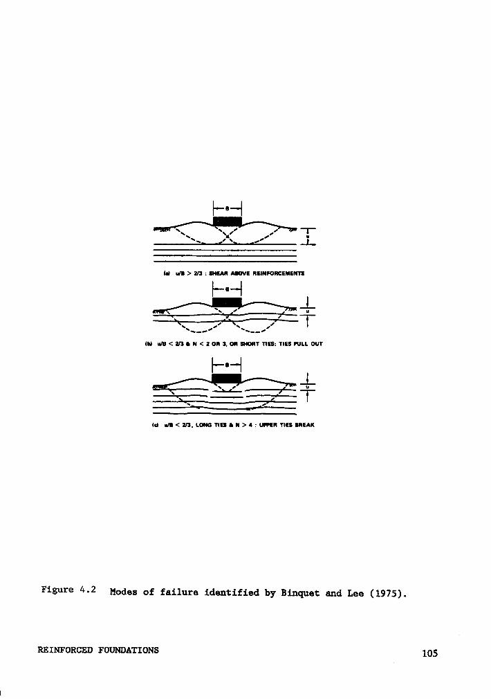
I—···|’ ‘ ·’
..1.
(II ul! > 2/3 : SNEAR AEVE REINFORCEMENTS|···—|„„ .... —
s 4, :s~,’(N
ll/B < 2/3 I N < 2 OR 3, Ol SHORT TIES: TIES FULL OUT
J--——%·—l-=ii. -·———¤——: Ji-
uIl<2l3.LONGTIESIN>l:UFFER TIESIREAK
Figure 4 • 2 Modes of failure identified by Biuquet and Lee (1975).
Rmuroxcxu roummrxous 1051
1. A minimum number of layers of reinforcing were required to obtain
significant load settlement and bearing capacity improvement, with
the the optimum number between four and eight layers.
2. The greatest improvement was obtained for an arrangement with the
reinforcing layers beginning at a shallow depth near the base of the
footing.
3. When the depth to the first layer of reinforcement was greater than
0.67 time the footing width, failure usually took place as shear above
the reinforcement rendering the effect of the reinforcement small or
nil.
4. In all cases where failure occurred by reinforcement breakage, the
broken spots were not located near the classical slip surface, but
rather in the upper layers, approximately below the edges of the
footing as shown in Figure 4.2c. In these cases punching shear type
failure surfaces were apparent.
The results of model test studies of reinforced cohesionless soils
using various reinforcing materials have also been reported by Akinusuru
and Akinbolade (1981), Fragaszy and Lawton (1984) and Guido et al. (1985a
and 1985b). All of these researchers have adopted Binquet and Lee°s
bearing capacity ratio terminology and have shown that various reinforc-
ing materials can increase the bearing capacity. In general, these test
results have substantiated the observations made by Binquet and Lee.
REINFORCED FOUNDATIONS 106
Little data has been published on the bearing capacity of reinforced
sands overlying weak, cohesive soils. Model test results have been re-
ported by Milligan and Love (1984), Jarrett (1984) and University of
California, Davis (1984b). In addition, Binquet and Lee (1975) performed
a few tests in which a soft zone was placed beneath the reinforced sand
by using foam rubber to simulate a weak clay layer. These tests have
shown that reinforced sand over weak clay provides increased bearing ca-
pacity compared to similar unreinforced systems, on the order of 50 to
100 percent. In the unreinforced tests run as controls, the mode offailure was always a punching failure of the sand into the clay. In the
reinforced tests the failure mode was less clearly discernible. With the
exception of the tests by Binquet and Lee, the tests were performed with
geogrids as the reinforcing material, and no slippage between the sand
and the geogrids or pullout of the geogrids from the sand was noted by
the researchers. The tests reported by Jarrett (1984) were conducted
using peat as the weak foundation soil.
In the model tests reported by Milligan and Love (1984), Jarrett
(1984) and University of California, Davis (1984b), where the sand was
reinforced with geogrids, the reinforcing was placed near the surface of
the weak clay or peat. The depth of fill was often greater than 0.67 times
the footing width, and yet failure did not occur above the reinforcement
as happened in the tests without a weak clay sublayer that were performed
by Binquet and Lee (1975). This suggests that the failure mechanism in
reinforced sand over weak clay is different than that for reinforced sand
without a weak clay sublayer. Thus, the trends observed by Binquet and
REINFORCED FOUNDATIONS 107
Lee for a minimum number of layers and placement of reinforcing layers
near the base of the footing may not hold for reinforced sand over clay.
Indeed, it is expected that concentrating the reinforcement near the
sand-clay interface will provide better results.
4.2.2 Analytical Techniques
4.2.2.1 Bearing Capacity of Unreinforced Cohesionless Soils Over Softb
Clay
The bearing capacity of unreinforced cohesionless soil overlying soft
cohesive soil has been studied by a number of investigators. For appli-
cation to the present study, the cohesionless layer is considered to be
relatively thin, so that the strength of the underlying clay controls the
l ultimate bearing capacity.
The bearing capacity for this condition has often been determined by
(a) computing the capacity as if the clay did not exist, and (b) computing
the capacity of a fictitious foundation (with an increased width) resting
directly on the clay, and using the smaller of these two bearing capaci-
ties. When this procedure in used, the increased width of the fictitious
foundation is often based on the load being distributed over a 2V:lH
projection area from the base of the footing (Terzaghi and Peck 1967).
The capacity of the system is controlled by the clay strength until the
depth to the clay becomes very large.
REINFORCED FOUNDATIONS 108
From research on the design of unreinforced aggregate layers over soft
soils for unpaved road systems, a clearer picture of the limitations of
the projected area method has developed. In such studies, the system is
subjected to a number of cycles of loading simulating loading by haul
trucks. Based on experimental model tests on aggregate over soft clay,
Bender and Barenburg (1978) adopted a pressure limit on the clay surface
of 3.3 times cohesion, with the pressure at the top of the clay being
determined from a Boussinesq stress distribution analysis. This pressure
corresponds closely with nc which can be considered as the elastic bearing
capacity of clay (Whitman and Hoeg 1966). Giroud and Noiray (1981),
Giroud et al. (1984) and Poran (1986) also adopted this limit for the
pressure exerted on the subgrade clay. The bearing capacity of the system
was then calculated by spreading the surface load to the clay surface by
the projected area method. The model test results of Milligan and Love
(1984) and University of California, Davis (1984b) support the limit of
nc as the bearing strength to use for unreinforced systems when using the
projected area method.
Experimental work by Tcheng (1957) (as reported by Vesic 1973) and
additional studies by Vesic (1973), as well as the model studies described
in the previous section, have shown that the mode of failure for this case
is punching along essentially vertical slip lines following the founda-
tion perimeter. The procedures based on the projected area methodology
do not consider this failure mechanism; instead, they consider a larger
critically loaded area at the surface of the clay.
REINFORCED FOUNDATIONS 109
l
To overcome this deficiency, Meyerhof (1974) proposed the following
approximate theory of the bearing capacity of a footing punching through
a thin, dense sand layer into a thick, soft clay bed. At ultimate load
a sand mass having an approximately truncated pyramidal shape is pushed
into the clay so that, in the case of general shear failure, the friction
angle ¢ of the sand and undrained cohesion c of the clay are mobilized
in the combined failure zones shown in Figure 4.3.
Meyerhof hypothesized that the forces on the failure surface in the
sand could be taken as equivalent to a passive earth pressure Pb inclined
at an angle 6 and acting upwards on a vertical plane through the footing
edge. For a strip footing of width B and depth D, at a distance H above
the clay surface, the ultimate bearing capacity was, approximately, given
by
qu = cNc + ZPP sin 6/B + yD [4.2]
where AQ= bearing capacity factor = 5.14 and y = unit weight of sand.
Meyerhof determined the passive earth pressure to be
Pp = 0.5yH2(1 + 2D)Kp/ cos 6 [4.3]
where Kb = coefficient of passive earth pressure.
The angle 6 decreases from about o near the footing edge to about zero
at the clay surface. Based on trial calculations, Meyerhof found an av-
erage value of 6 to be in the range of to Ääl and recommended that avalue of be used. In addition, it was recommended for practice to
use a coefficient Kxof punching shearing resistance on the vertical plane
REINFORCED FOUNDATIONS 110
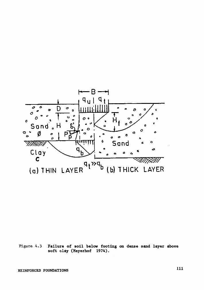
1**B **1qu! qt
°,° cn Ü °„ ’ —• 6 o 6
Og ° "° 1 ¤ ° O 6 T 6°
O Ö •Ö .6 .
° 7 Ü•
¢ ‘
Sond o H 8•= oo
"WTY1 ‘*Sund ¤ ‘· .
Clgy . «° ° 6 6 6 ¢>
C
LAYER tb) 11-ucx LAYER
Figure 4.3 Failure of soil below footing on dense sand layer abovesoft clay (Meyerhof 1974).
Rzmroucsu 1=ouN1:>A*r1oNs 111
through the footing edge such that, on substitution of Equation 4.3 into
Equation 4.2, the bearing capacity becomes
qu = cNc tan 9/B + yD [4.4]
where
Kstan9= Kpzanö [4.5]
and R} is a coefficient of punching shear. A maximum bearing capacity
equal to the ultimate bearing capacity of the sand was recommended as an
upper limit on Equation 4.4.
The value of R} is difficult to determine. Meyerhof presented values
‘ of Ag determined using Equation 4.5 and earth pressure coefficients kb
based on logarithmic failure surfaces as functions of 9. Values of R}
determined from limited model testing and field records were compared to
values calculated from theory for 8 = 0.69 and found to be in good
agreement.
The analysis was extended to circular and rectangular footings by
determining the passive resistance Pb inclined at 8 on vertical surfaces
through the footing perimeter, with the increased resistance for these
cases expressed through shape factors applied to Equation 4.5.
The theory as described above has been compared to bearing capacity
tests on model footings and found to be in good agreement. Additional
work on the determination of the coefficient of punching shear Rg was
presented by Hanna and Meyerhof (1580). This work provided for consid-
erably reduced punching shear coefficients when the undrained strength
REINFORCED FOUNDATIONS 112
of the cohesive layer was less than 10 kPa (200 psf). In addition, an
extensive set of charts for the determination of K} was presented. Kraft
and Helfrich (1983) compared this theory to the results of 27 full-scale
and model bearing capacity tests and found very good agreement between
measured and predicted bearing capacity. Kraft and Helfrich concluded
that the theory was of such merit as to recommend discontinuing the use
of the 2:1 pressure method for calculating bearing capacities for sands
overlying soft clay. Additional support for Meyerhof's theory is pre-
sented in Figure 4.4, where the measured and calculated bearing capacity
of unreinforced model tests from Milligan and Love (1984) and University
of Califcrnia, Davis (1984b) are compared. It can be seen that quite good
agreement is obtained. The data which do not show a particularly good
fit are from tests on very weak subsoils (Sh less than 10 kPa), and for
these soils the reductions in R} proposed by Hanna and Meyerhof (1980)
may be too severe.
4.2.2.2 Bearing Capacity of Reinforcad Cobesionless Soils Over Soft Clay
Because the reinforcement of sands over weak clays is a relatively
new development in geotechnical engineering, the literature devoted to
bearing capacity analysis is scant. The papers of Bender and Barenburg
(1978), Giroud and Noiray (1981), Giroud et al. (1984), Milligan and Love
(1984) and Poran (1986) form the groundwork of the literature devoted to
this subject.
REINFORCED FOUNDATIONS 113
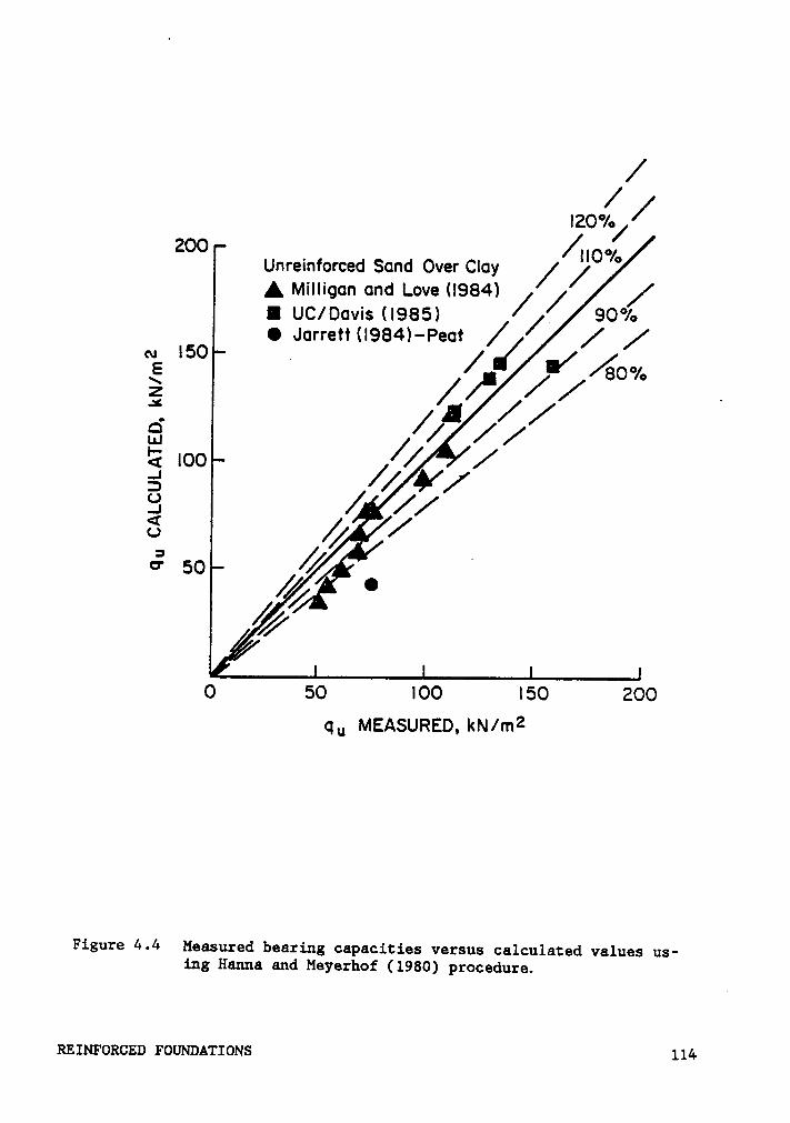
//I20°/• /
//ZOO 1 I|O°/¤Unre1nforced Sond Over Cloy / /
A Milligon ond Love (I984)/ / /I uc/0¤v1s(19a51 / 90%
O Jorrett (I984)—Peot / / /
g 4//;/ 13 /// //'E 100 / / /5°ä / //Ö 50 /Ü
·°
/ /
0 50 100 150 200Qu MEASURED, kN/mz
Figure 4.4 Measured bearing capacities versus calculated values us-ing Hanna and Meyerhof (1980) procedure.
REINFORCED FOUNDATIONS 114
From these works, the major effects of reinforcement for improving
bearing capacity appear to be:
1. Increased confinement of the cohesionless layer (Bender and Barenburg
1978) and of the subgrade material (Giroud et al. 1984), providing
enhanced bearing capacity of both of these materials.
2. Alteration of the failure mechanism in the soft soils by distributing
stresses more evenly over the soft soil (Bender and Barenburg 1978
and Giroud et al. 1984).
3. A tensioned. membrane effect which results in a reduction of the
pressure applied to the subgrade soil (Giroud and Noiray 1981).
In addition, the presence of a geotextile or geogrid at the sand-clay
interface reduces intermixing of the sand and clay, which can have det-
rimental effects on the performance of both materials.
Bender and Barenburg (1978), Giroud and Noiray (1981), Giroud et al.
(1984) and Poran (1986) have all assumed that the effective confinement
induced by the reinforcement increases the bearing capacity of the clay
from the value of nc applicable to brittle materials (see previous sec-
tion) to the value of Q + ny applicable to ductile materials. Exper-
imental evidence for this was first presented by Bender and Barenburg
(1978). Hence, all of the referenced studies indicate that the limiting
bearing pressure on the clay subgrade under reinforced cohesionless lay-
ers can be taken as Q + ny. The bearing capacity of a reinforced system
REINFORCED FOUNDATIONS 115
can then be determined using procedures for calculating the load dis-
tributed to the clay, where the limiting pressure on the clay is
(2 + 1:)c. All of these procedures considered a single layer of re-
inforcement at the base of the cohesionless layer. Giroud and Noiray •
(1981) and Poran (1986) made theoretical calculations of the tensioned
membrane effect contribution to the bearing capacity, and determined that
it was negligible.
The procedures described above have the shortcoming that they are
limited to a single layer of reinforcement placed at the base of the
cohesionless layer, and that no direct consideration of the strength of
the reinforcement is contained in the procedures. It is therefore not
possible to determine the required quantity or strength of the re-
- inforcement by means of these procedures.
4.3 Finite Element Analyses
In contrast to reinforced embankments, the analysis of reinforced
foundations using the finite element method has received little atten-
tion. The publications by Brown and Poulos (1981) and Poran (1986),
appear to be the only previous work on application of the finite element
method to reinforced foundations.
Brown and Poulos (1981) performed a finite element analysis of the
experimental model tests performed by Binquet and Lee (1975). The details
of the model used are the same as those described in Chapter 2 for the~
authors work on reinforced embankments (Brown and Poulos 1978). Their
REINFORCED FOUNDATIONS 116

analyses showed that the reinforcement had little effect on the elastic
stiffness of the footings. This was in contrast to Binquet and Lee°s test
results which indicated an increased stiffness with increasing amounts
of reinforcement. The analyses did indicate a significant increase in
collapse load and smaller deformation to failure with increasing amounts
of reinforcement. However, the analyses consistently underpredicted the
collapse load compared to the experimental results. A comparison of
plastic regions in the unreinforced and reinforced analyses showed that
the presence of reinforcement spread the footing load and caused a deeper
and wider mobilization of soil strength.
Poran (1986) performed two-dimensional, plane strain finite element
analyses of them model tests that had been performed at the Unversity of
California, Davis (1984b). In his analyses he used a bounding surface,
elasto-plastic model (Dafalias and Herrmann 1982) and special reinforcing
elements developed by Hermann (1984). Load-displacement curves from the
finite element analyses indicated smaller loads than the model test
curves. Poran attributed the differences to the three-dimensional geom-
etry of the model tests. Poran applied a correction factor based on shape
factors for two- and three-dimensional geometries to reduce the model test
results to two-dimensional conditions and obtained much better agreement
between calculated and experimental load-displacement curves. In ana-
lyses of model tests without that had been performed without reinforce- pment, the analyses indicated that failure should occur by localized
punching of the sand into the c1ay,the same mechanism of failure as ob-
served in the model tests. With the addition of reinforcement, the mode
REINFORCED Fouwmrxous 117
of failure was less distinct in both the model tests and the analytical
results. The failure area extended laterally away from the footing, en-
gaging significantly more volume of soil in the failure compared to the
unreinforced case.
In this study, additional finite element analyses of the model test
performed at the University of California, Davis (1984b) were performed.
The University of California, Davis model tests were performed in a wooden
box 73 inches long, 68 inches wide and 48 inches high. A saturated clay 1
sample 26 inches high was formed in the box and an eight inch thick sand
layer was placed on top of the clay. The footing load was applied through
a 12-inch square, 1-1/8 inch thick steel plate using a hydraulic jack
system. Tensar SS1 was used as the reinforcement, and was placed in the
sand two inches above the clay.
The computer programs describe in Chapter 3 were used in the analyses,
and both plane strain and axisymmetric analyses were performed. The fi-
nite element analyses modeled a symmetrical half of the model test box,
and used 35 elements to represent the clay and 36 elements to represent
the sand. The mesh was finer near the footing and larger elements were
used away from the footing. The reinforcement was modelled using the
elements described in Section 3.4.2. It seems likely that the greatest
uncertainties in the analyses arise from the selection of material prop-
erties for the clay, the sand and the reinforcement. Little data on the
soils was contained in the University of California, Davis report. The
only data available were the friction angle of the sand, cohesion values
for the clay determined from unconfined compression tests, and gradation
REINFORCED FOUNDATIONS 118
and classification tests on the sand and clay. These data were used to
estimate soil strength parameters for the finite element model following
the guidelines of D°0razio and Duncan (1982), and Section 3.4.
Compressibility parameters were determined by trial, attempting to
achieve the best possible match between the load-deformation curve com-
puted in an axisymmetric unreinforced analysis and that measured in the
unreinforced model tests.
The initial soil stresses and the preconsolidation pressures are also
important for the finite element analyses. The preconsolidation pressure
for the clay soil was estimated using the procedure described in Section
3.4. The saturated clay was assumed to have R% = 1 initial stress con-
ditions.
The initial stresses for the sand were more difficult to estimate.
The only information available was that a high pressure pneumatic vibro-
plate compactor was used to compact the sand. Preliminary analyses using
Kb = 1 in the sand resulted in failure under loads of 400 lbs (compared
to failure loads of about 2800 lbs in the model tests) and were therefore
deemed unrepresentative of the actual conditions. Next, the initial
stresses were computed using the procedures for estimating compaction-
induced stresses developed by Seed and Duncan (1983). The use of these
compaction·induced stresses produced load-displacement curves which were
extremely stiff and which greatly overpredicted the load-settlement be-
havior of the model tests. By trial, it was found that R%==2 stresses
in the sand gave a reasonable match between the unreinforced model tests
and the finite element results.
REINFORCED FOUNDATIONS 119
The value of stiffness for the Tensar SS1 reinforcement was determined
from load-strain plots presented by Tensar (1983) and the values of
measured strain reported by University of California, Davis (l984b).
Average values of measured strain in the reinforcement varied from 0.8
to 1.8 percent in the model tests. A strain of two percent was selected
for determining the value of modulus to input into the analyses. At two
percent strain, the modulus was calculated to be 2000 lb/in in the strong
direction and 1150 lb/in in the weak direction. The plane strain analyses
of the axisymmetric tests were run using an average of the stiffness in
the two directions. The axisymmetric analyses used an equivalent modulus
in the membrane element, determined using the procedures described in
Appendix B. The value of this modulus was E = 1440 lb/in.
The dashed lines in Figure 4.5 show typical load—footing displacement
results from the unreinforced and the reinforced model tests. It can be
seen that no footing displacement was measured until approximately 400
pounds of load were applied to the model footing. It can also be seen
that the reinforced model test carries only slightly larger loads than
the unreinforced model test, up to a footing displacement of approximately
one inch. Above this footing displacement, the load carrying capacity
of the reinforced system increased significantly. It would appear from
this results that a critical amount of deformation is required to mobilize
the behavior of the reinforcement.
The results of the plane strain finite element analyses of the model
tests are shown in Figure 4.5 and the results of the axisymmetric analyses
are shown in Figure 4.6. It may be seen that the plane strain analysis
REINFORCED FOUNDATIONS 120
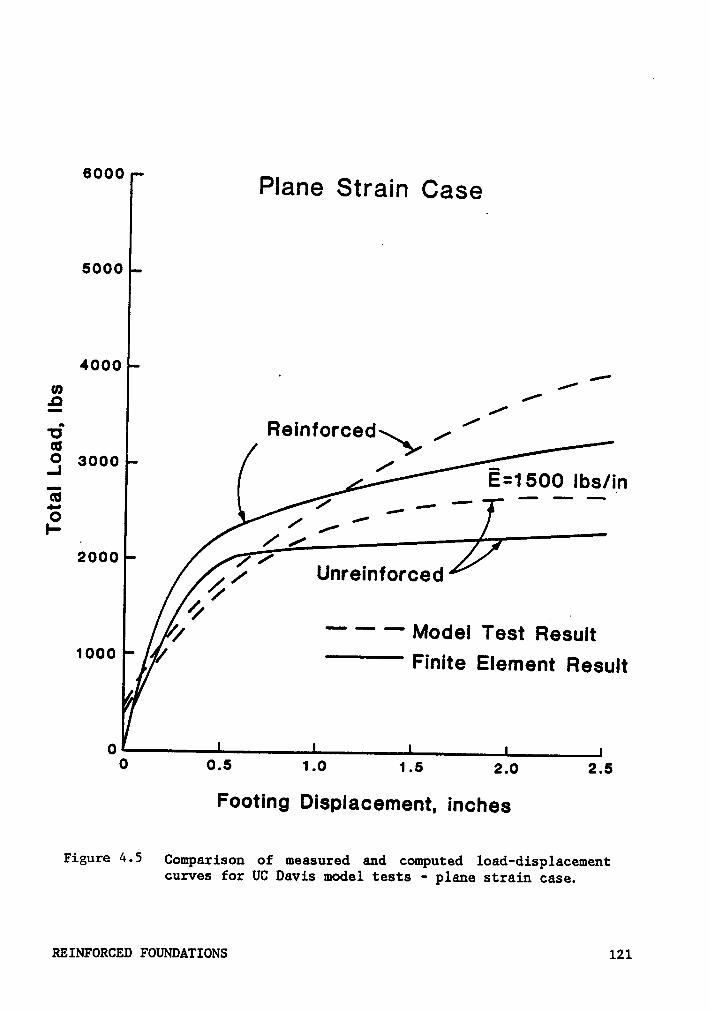
6000 .Plane Stram Case
60004000 _ Im (2 / /· Reinforced /
U Z2 \*0 / -
:_‘E=1500 lbs/in
g ’ „ r "’ ” -/ /P . / /
2000 / _Unremforced//Ö _ .
/ ** "' — Model Test Result‘°°° / ‘* Finite Element Result
0 0 0.6 1.0 1.5 2.0 2.5Footing Displacement, inches
Figure *-5 Comparison of measured and computed load-displacementcurves for UC Davis model tests - plane strain case.
Rxxuroxczv Fouunarxous . 121

of the reinforced case underpredicts the ultimate load of the model test.
It has been found previously by Meyerhof (1974) and others, that plane
strain analyses of bearing capacity result in smaller failure loads than
measured in circular plates and this result is thus as expected. The
initial load-deformation behavior is modelled reasonably well considering
the model test required some 400 pounds of load application before meas-
urable movements occurred. The computed load-displacement curve is
somewhat steeper than the model test curve but is in reasonable agreement.
The plane strain reinforced analyses also underpredicted the rein-
forced model test results. The computed results indicate that the addi-
tion of reinforcement would be expected to cause a steepening of the
load-displacement response in the early part of the test, and increase
the ultimate load. The differences between the computed unreinforced and
reinforced behavior are comparable to the differences exhibited in the
model test results, showing good qualitative agreement with the model
tests.
The results of the axisymmetric finite element analyses of the model
tests are shown in Figure 4.6. The model parameters used in the analyses
were chosen such that the calculated collapse load and load-deformation
behavior for the axisymmetric case would agree as well as possible with
the model test results. It can be seen that the calculated collapse load
agrees very well with the measured collapse load. However, achieving a
match of the load-deformation curves was not as easy. The load-
deformation curve shown in Figure 4.6 is about the best match for the
unreinforced load test that could be achieved after several trials.
REINFORCED FouN¤A*r1oNs 122
1
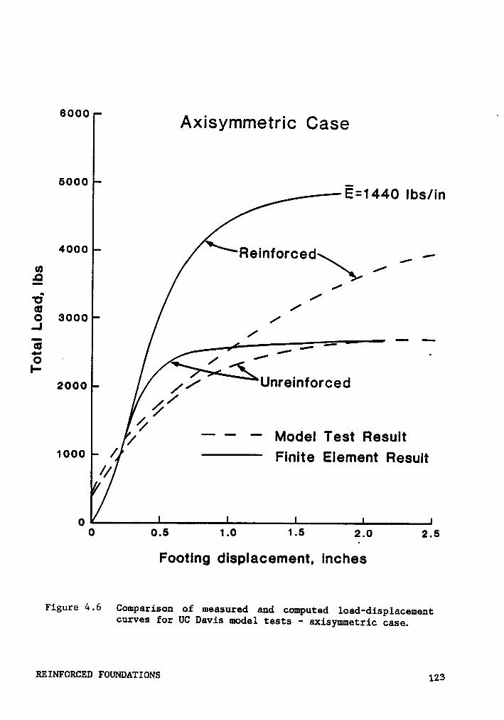
6000 . . ‘AXISYITITTIGTTIC Case
5000 — _E=1440 lbs/in
‘*°°° ‘*Reinforced .-"’ /2 /
· /Q /O 3000 /.l / _ —
l" .I2000 // Unremforced
/44/ — — ·— Model Test Result
1¤0¤ / —l·· Finite Element Result//
00 0.5 1.0 1.5 2.0 2.5
Footing displacement, inches
Figure 4.6 Comparison of measured and computed load-displacementcurves for UC Davis model tests - axisymmetric case.
REINFORCED FOUNDA'1‘IONs 123
II
Subsequent to the initial movement, the measured load-displacement curve
is somewhat flatter than the calculated curve.
The analysis of the reinforced case shows a much higher ultimate
strength and a considerably stiffer load-displacement response. It can
be seen that the reinforced and the unreinforced computed curves are
identical up to a load of about 1500 lbs. This indicates that the re-
inforcement has little effect on the calculated behavior until nearly
two-thirds of the unreinforced collapse load is reached. The computed
results indicate that the reinforcement should greatly increase the
load-carrying capacity. However, this is not in agreement with the
measured results, which show a much smaller increase in load capacity at
similar values of footing displacement. Additionally, the computed
load-displacement response is significantly stiffer than measured re-
sponse. This is likely due to the selection of soil properties, which
required several assumptions, and the effect of the test box boundaries.
In addition to the load-deformation results, the following observa-
tions were made of the computed results:
1. In the unreinforced analyses, failure initiated at the bottom of the
sand layer and progressively spread upward and outward through the
sand. Punching failure occurred in the clay elements once the sand
had failed. The punching failure occurred only in those elements
directly under the footing. This mode of punching failure was con-
sistent with the observed failure mode in the model tests.
Rmuroxzcan Fou1~mA1·1o1~1s 124
2. In the reinforced analyses, failure began in elements above the re-
inforcement and did not spread to elements below the reinforcement
until elements between the reinforcement and footing had failed. The
zone of failed elements was much wider in both the sand and clay
compared to the unreinforced analyses, and the punching mode of
failure was not evident. The shear stress was reduced 20 to 40 per-
cent at comparable stages of loading in the upper layer of clay ele-
ments.
The foregoing discussion of the computational results indicates that
the finite element analyses provide reasonable qualitative agreement with
measured behavior. In addition, the results are in quantitative agreement
when allowance is made for the uncertainty in several of the soil prop-
erties used in the analyses. In particular, the effects of soil
compressibility on reinforced soil behavior requires further investi-
gation, and an improved understanding of initial stress conditions in soil
would probably improve the analyses. The axisymmetric finite element
progrmm appears to provide a useful tool for the analysis of three-
dimensional reinforced soil-foundation problems.
REINFORCED FOUNDATIONS 125
l
4.4 A Proposed Method for Bearing Capacity Analysis of Reinforced Sand
Over Weak Cohesive Soils
4.4.1 Postulated Mechanisms of Failure
In the model tests reviewed in Section 4.2.1, the predominant failure
mechanism observed was punching shear failure through the sands. In light
of this, it is considered appropriate to develop a bearing capacity theory
based on the punching shear mode of failure. In addition, an approach
which incorporates the strength of the reinforcement in the procedure in
a direct manner is highly desirable. Two possible deformation mechanisms
are shown in Figure 4.7. The first involves punching shear whereby the
footing, the sand, and the reinforcement punch into the clay in much the
same manner as in the unreinforced case. For this mechanism, the addi-
tional capacity due to the reinforcement must, as an upper bound, be the
tensile strength of the reinforcement.
The second mechanism involves a more general shear failure whereby
the reinforcement is deformed in the manner shown in Figure 4.7b. The
increase in capacity compared to the unreinforced case is considered to
occur through the effects of increase in confining pressure due to the
reinforcement. This occurs because, as load is added to the system, the
reinforcement increases the effective confining pressure in the sand, and
hence its strength.
REINFORCED FOUNDATIONS 126
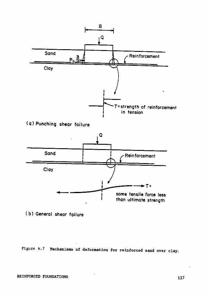
l·—l—1Q
$¤l"dS Reinforcement-°p
Clay
.
1
_ $strength of reinforcement1 in tensionl
la) Punching shear failure
Q
I .Sand1 l Relnforcement
Clay•——
1 some tenslle force lessI than ultimate strength
lb) General shear failure
Figure 4-7 Mechanisms of deformation for reinforced sand over clay.
Rzmroxzcmw FOUNDATIONS V 127
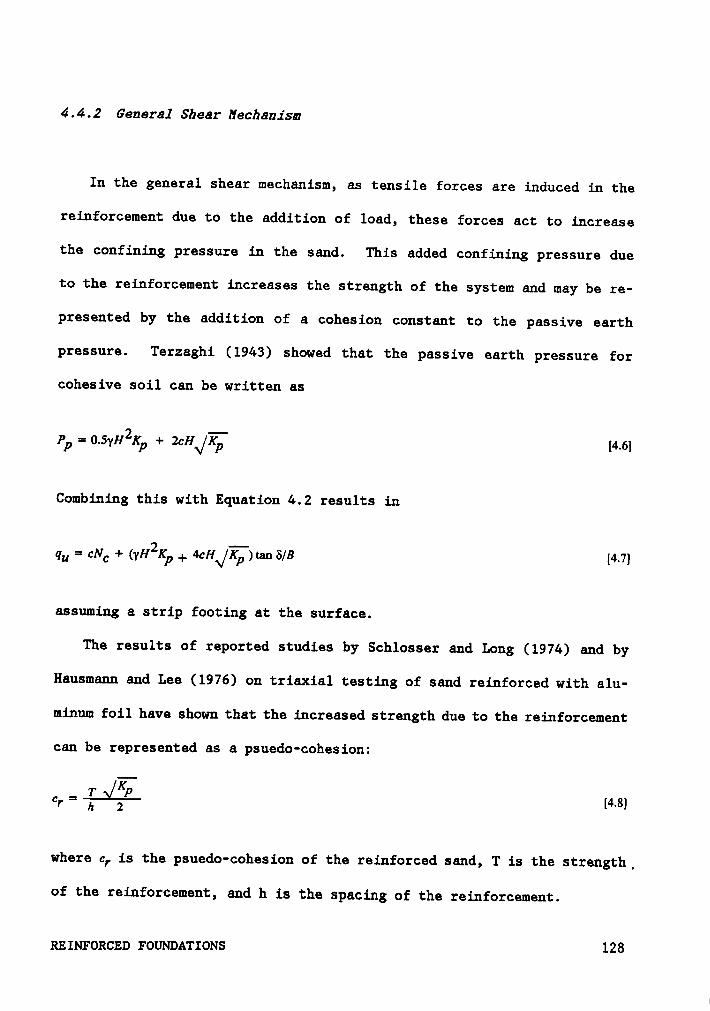
4.4.2 General Sbear Hecbanism
In the general shear mechanism, as tensile forces are induced in the
reinforcement due to the addition of load, these forces act to increase
the confining pressure in the sand. This added confining pressure due
to the reinforcement increases the strength of the system and may be re-
presented by the addition of a cohesion constant to the passive earth
pressure. Terzaghi (1943) showed that the passive earth pressure for
cohesive soil can be written as
- 2 *Pp — 0.5yH Xp + 2cH\/KP [4.6]
Combining this with Equation 4.2 results in
qu = cNc + (yH2Kp + 4cH\/Ehan 8/B [4.7]
assuming a strip footing at the surface.
The results of reported studies by Schlosser and Long (1974) and by
Hausmann and Lee (1976) on triaxial testing of sand reinforced with alu-
minum foil have shown that the increased strength due to the reinforcement
can be represented as a psuedo·cohesion:
er [4.8]
where q.is the psuedo-cohesion of the reinforced sand, T is the strength_
of the reinforcement, and h is the spacing of the reinforcement.
REINFORCED F0UNDA1‘10Ns 128
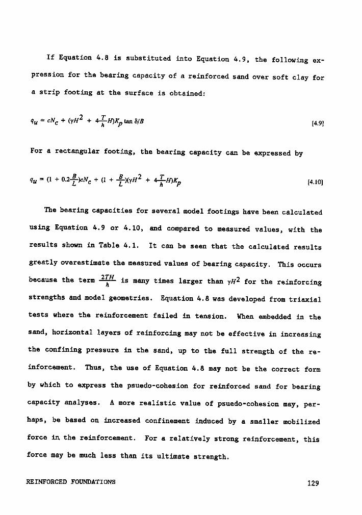
If Equation 4.8 is substituted into Equation 4.9, the following ex-
pression for the bearing capacity of a reinforced sand over soft clay for
a strip footing at the surface is obtained:
qu = cNc + (yH2 tan 5/B [4.9]
For a rectangular footing, the bearing capacity can be expressed by
qu = (1 (1 [4.10}
The bearing capacities for several model footings have been calculated
using Equation 4.9 or 4.10, and compared to measured values, with the
results shown in Table 4.1. It can be seen that the calculated results
greatly overestimate the measured values of bearing capacity. This occurs
because the term éggi is many times larger than yH2 for the reinforcing
strengths and model geometries. Equation 4.8 was developed from triaxial
tests where the reinforcement failed in tension. When embedded in the
sand, horizontal layers of reinforcing may not be effective in increasing
the confining pressure in the sand, up to the full strength of the re-
inforcement. Thus, the use of Equation 4.8 may not be the correct form
by which to express the psuedo-cohesion for reinforced sand for bearing
capacity analyses. A more realistic value of psuedo-cohesion may, per-
haps, be based on increased confinement induced by a smaller mobilized
force in the reinforcement. For a relatively strong reinforcement, this
force may be much less than its ultimate strength.
REINFORCED FOUNDATIONS 129
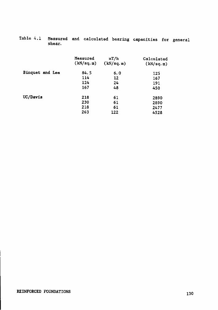
Table 4.1 Measured and calculated bearing capacities for generalsheax.
Measured nT/h Calculated(kN/sq.m) (kN/sq.m) (kN/sq.m)
Binquet and Lee 84.5 6.0 125114 12 167124 24 191167 48 450
UC/Davis 218 61 2890230 61 2890218 61 2477263 122 4528
REINFORCED FOUNDATIONS 130
It appears that development of a logical method for determining a
suitable psuedo-cohesion for bearing capacity analyses must await addi-
tional experimental work. In this regard, the large-scale plane strain
apparatus developed by Dove (1986) could provide the necessary means.
In this equipment true-scale geogrids and geotextiles can be used to re-
inforce sand. Results from such tests would shed considerable light on
the increases in strength that could be expected for the failure mechanism
described here. If such testing confirmed realistic values of psuedo-
cohesion, Equation 4.6 could be used for the passive earth pressure and
the graphical techniques outlined by Hanna and Meyerhof (1980) could be
extended to develop curves for reinforced sand over clay based on the
strength of the clay and the psuedo-cohesion of the sand.
4.4.3 Puncbing Sbear Hecbanism
The mechanism envisioned is shown in Figure 4.7a. At failure the re-
inforcement is deformed such that the full tensile resistance of the re-
inforcement is mobilized to support the load. At failure the
reinforcement either breaks or pulls out from the sand due to failure of
the bond between the reinforcement and the sand.
The increase in bearing capacity is taken to be the strength of the
reinforcement. When this added resistance is factored into Meyerhof°s
theory, the ultimate bearing capacity can be expressed as:
qu = cNc + yH2K_‘.tanq>/B + 2"EZ- [4.11]
REINFORCED Fouumrxous 131
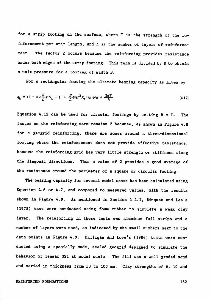
for a strip footing on the surface, where T is the strength of the re-
inforcement per unit length, and n is the number of layers of reinforce-
ment. The factor 2 occurs because the reinforcing provides resistance
under both edges of the strip footing. This term is divided by B to obtain
a unit pressure_for a footing of width B.
For a rectangular footing the ultimate bearing capacity is given by
qu = (1 + 0.2·%)cNc + (1 + %)yH2K_‘.r.an <p/B + -2-%,- [4.12]
Equation 4.12 can be used for circular footings by setting B = L. The
factor on the reinforcing term remains 2 because, as shown in Figure 4.8
for a geogrid reinforcing, there are zones around a three-dimensional
footing where the reinforcement does not provide effective resistance,
because the reinforcing grid has very little strength or stiffness along
the diagonal directions. Thus a value of 2 provides a good average of
the resistance around the perimeter of a square or circular footing.
The bearing capacity for several model tests has been calculated using
Equation 4.6 or 4.7, and compared to measured values, with the results
shown in Figure 4.9. As mentioned in Section 4.2.1, Binquet and Lee's
(1975) test were conducted using foam rubber to simulate a weak clay
layer. The reinforcing in these tests was aluminum foil strips and a
number of layers were used, as indicated by the small numbers next to the
data points in Figure 4.9. Milligan and Love's (1984) tests were con-
ducted using a specially made, scaled geogrid designed to simulate the
behavior of Tensar SS1 at model scale. The fill was a well graded sand
and varied in thickness from 50 to 100 ~«. Clay strengths of 6, 10 and
} REINFORCED FOUNDATIONS 132
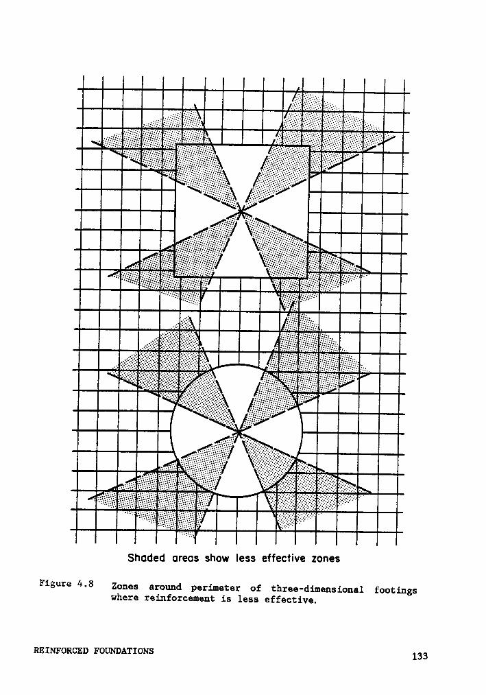
IIIIIIIIII
Ellllü‘:--i IllllIII-Illl!
ellläll
IIIIIIIIIIIll!@e@lII¤ee%!¤l
·lliüääälllwällllShoded oreos show less effective zones
Figure 4-8 Zones around perimeter of three-dimensional footingswhere reinforcement is less effective.
REINFORCED FOUNDATIONS 133

300 _ /l2Rennforced Sand Over Clcy - / /O Binquet und Lee II975) *20o// /A Mauagqn und Love (|964) / *°*O{/ //
250 I UC/Davis (I985) / 90% // / / 2. / /0‘“ / / / /E 200 8 / /~
•( /Z / /x K /. /6 / /LU /I; Iso / ////..1 / 4 /D ’, /3 A 3/ /5 /100 4/ •//S 6 64
/& Smoll numbers refer Io number50 of relnforcing Ioyers.
Ü// No number = I I¤yer///
50 I 00 I 50 200 250 300
qu MEASURED, kN/mz
Figure [M9 Measured bearing capacities versus calculated values forthe reinforced case using Equation 4. 6 or 4. 7.
Rmurouczm FOUNDATIONS *13,*
16 kPa were obtained by consolidating slurried kaolinite. In all their
tests the geogrid was placed at the sand-clay interface. The tests by
Binquet and Lee, and by Milligan and Love were conducted using strip
footings. The tests conducted by University of California, Davis (1984b)
used a one—foot-square plate and eight inches of sand or gravel over a
soft, organic clay having an average Sh of 15 kPa (310 psf). In these
tests, Tensar SS1 geogrid was placed two inches above the clay surface.
In tests with two layers, the second layer was placed two inches above
the first. The strength of the reinforcement used in calculating the
bearing capacity was taken as the tensile rupture strength reported by
the investigators. In the case of the University of California, Davis
tests, the strength was considered to be the quality control value of
tensile strength from Tensar literature. Because it is a biaxial geogrid,
the strength of SS1 is different in the two directions. For the data
shown in Figure 4.9, the tensile strength used was the minimum value in
the two directions. Calculated bearing capacity values using the maximum
strength were approximately 20 percent higher. A compilation of the
footing width, depth of sand fill, shear strengths, reinforcement
strength and number, and the measured and calculated bearing capacities
is presented in Table 4.2.
Despite the apparent simplicity of the approach, quite good agreement
is obtained between measured and calculated results. Although refine-
ments may be indicated by further test results, the method appears I68'
sonable for practical use in design. Application to one field case,
REINFORCED FOUNDATIONS 135
i
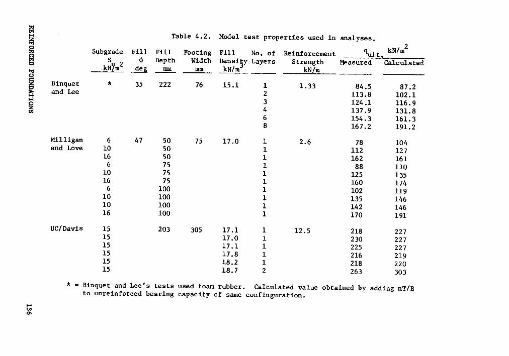
*:1GJJä
Nr-O
EIJw
O•-•M
~¤
¤~
CN
\0¤
·I¢"’7
f\•-|<I'<
!'G\
NN
N•—
•NO
GN
NN
NN
Mco
MG'¤
SCD
HQ
'¢"7
<f|\<
f|\®
NN
®Ih
ON
l-H
NO
QO
I-¤\D
®¢
"'!
„-D!>«
GN
NN
NN
N*3
GG
Gg:
uu
·•-JG
.-GGJ
O"U
E-G
aa0
4-•E
<vua
u¤
0\
<'•'>:1
"S
SE
"*‘°
"‘Té
U1*4
-IHv-4
NN
>¢
GJG
ue-I
OE
"5"’BE
*5°‘
*5.*3D
-•-I'-7
8°‘52
5é°G-u
ow
Us:
rnz•-1
o>~
·UI-I6
HG
)-4
•¤-GE
«-4O
«-4
c•—
IwN
l~C
DE
Q,.4
q;\
•„
..
•-
„-
am
•¤•—
•GZ
nnr~
r~r~
r~r~
co
¤¤
„¤¢
nO
••-48
3•-4
•-••-•¤
-4--4
•-Jr-I-I
IJE
Fus-·-EE
.4.%°.·‘.%
äh•
·«-omg»o
mnnn
¤-e-•-•q·
un-4r~
r~O
05
83°°
Bä
•-4ke
UJGJ„-g
SO
[—•„G
¢¤¤¤v-I4-JE
NG
OG
!-HI-hl-FSO
OO
OG7
4-IG«
-•G-
NO
mw
-4·•-IG
JN
¤-In-~|•—Iv-O
NG
J}-JPr-«¤
Ua
!}
Htn-G
•-4-9
-GJ
mn
r~G
J*¤••-•
*¤M
<r
GJG
JFu
•-13
E5?.+*.122
*6n
mz
-l¢~
DO
\D~
0O
~D
xO
OO
~D
nn
un
mm
mu
nu
mBJ3
:.1¤‘G
cnG·«
-•O
Gm
¤¤
uJJG
Jm
g••·|
IIG
JGJ
GD
O>
3.-1
·¤-••-1¢G
-k¤
'r—
IQ
G·'¤
•-4*U\
·••-JG
·v-IGU
EGG
!zw
::>
REINFORCED
FOUNDATIO
NS136
described below, indicates the method provides results in reasonable
agreement with observed field behavior.
In a study of the performance of a Tensar SSl reinforced haul road,
Barksdale and Prendergast (1985) reported punching shear failure of re-
inforced and unreinforced crushed stone fills at fill thicknesses of 610
mm (24 inches). The unreinforced fill failed upon initial loading whereas
the geogrid reinforced section failed on the sixth pass of a loaded C-65
Chevrolet dump truck, with the geogrid breaking under the load. The re-
port indicated that the subgrade strength where the reinforced failure
occurred was low for this site and averaged 5.5 kPa (115 psf). The
bearing capacity for the reinforced section has been calculated using
Equation 4.6 and a friction angle of 50° for the crushed stone fill (based
_ on reported densities and CBR values). The bearing capacity determined
was 500, 540 and 575 kPa using tensile strengths for SS1 corresponding
to the minimum, average and maximum values of quality control strength
of SS1, respectively. For the contact area and weights reported by
Barksdale and Prendergast (1985) for the loaded C-65 dump truck, the load
causing failure was about 560 kPa. This provides a single field data
point in good agreement with the proposed method.
4.5 Summary
In this chapter, the problem of foundations constructed on reinforced
soils overlying weak subsoils has been analyzed using the finite element _
method and a modified bearing capacity procedure. An axisymmetric program
REINFORCED FOUNDATIONS 137
for analysis of reinforced soil problems provides a capability for ana-
lyzing circular footings on reinforced soil layers. Comparison of the
results of finite element analyses with experimental results from model
footings on reinforced sand overlying weak clay show that good qualitative
agreement can be obtained for load-displacement curves and for modes of
failure. The analyses show that the reinforcement has the effect of
spreading out the load over a wider area, thus reducing the shear stresses
occurring in the clay, which allows larger loads to be carried by the clay
before failure occurs.
A new procedure for computing the bearing capacity of reinforced sand
over weak soils has been proposed. The procedure is based on a punching
shear deformation mechanism. The method considers the strength and the
number of layers of reinforcement in a rational way. Comparisons with
several model test studies shows that the procedure provides good pred-
ictions of the ultimate bearing capacity of reinforced sand over weak
soils. The method is superior to previously developed procedures in that
it accounts explicitly for the reinforcement strength and the number of
layers.
The above described methods provide procedures for computing the ul-
timate capacity of reinforced sand over weak soils, and for computing the
load-deformation behavior of these systems. By using these two procedures
together, reinforced foundations over weak soils can be designed with some
confidence.
iREINFORCED FOUNDATIONS 138
CHAPTER V
EVALUATION OF THE BEHAVIOR OF HOHICANVILLE DIKE NO. 2
5.1 Introduction
This chapter describes the application of the finite element tech-
niques described in Chapter III to the analysis of Mohicanville Dike No.
2, a 28-foot high flood control dike reinforced with steel wire mesh.
The scope of the study described in this chapter included an analysis of
the instrumentation data collected during and shortly after construction,
a finite element analysis of the dike, and comparisons of the calculated
and measured results.
5.2 Background
Mohicanville Dike No. 2 is a rim dike on the Mohicanville Reservoir
in Wayne County, Ohio. Constructed by the U. S. Army Corps of Engineers,
the dike is 28 feet high and about 1800 feet long. Originally constructed
beginning in 1936, the dike suffered a number of failures during con-
struction, and could not be raised above 12 feet, owing to the very low
strength of the peat and clay foundation at the site. Subsequent
settlement reduced its height to about ten feet, and it was maintained
at this height, about 18 feet below design grade, until its reconstruction
in 1984 and 1985. A typical cross-section is shown in Figure 5.1 where
EVALUATION OF TIE BEHAVIOR OF MOHICANVILLE DIKE NO. 2 139

the foundation conditions and the bounds of the old and new embankments
are delineated.
A number of alternatives for raising the dike were evaluated in the
late 1970's by Law Engineering Testing Company for the Huntington District
to determine the most feasible method of raising the dike to its design
height (Collins et al. 1982). Because of the very low strength of the
foundation soils, construction of a conventional embankment was infeasi-
ble, no matter how flat the slopes. The depth of the peat and clay was
so great (about 60 feet) that excavation of the weak materials was not
economically feasible. Displacement of the soft foundation soils was
considered, but was rejected because of the extremely large quantities
of fill required, and the uncertain quality of the resulting structure.
Use of a concrete flood wall was considered but rejected because of the
very poor foundation support. Eventually it was decided that the best
alternative for raising the dike would be construction of a reinforced
embankment.
The use of reinforcement to improve embankment stability is fairly
new, and design procedures are still being developed. In the case of
Mohicanville, both finite element analyses and couventional equilibrium
slope stability analyses were performed. The slope stability studies were
performed by Law Engineering Testing Company (Collins et al. 1982) and
the finite element analyses were performed by the U.S. Army Waterways
Experiment Station in conjuction with Prof. J. M. Duncan (Fowler et al.
1983). The finite element analyses were used to estimate the force in
the reinforcing and the horizontal and vertical movements of the
EVALUATION OF THE BEHAVIOR OF MOHICANVILLE DIKE NO. 2 140
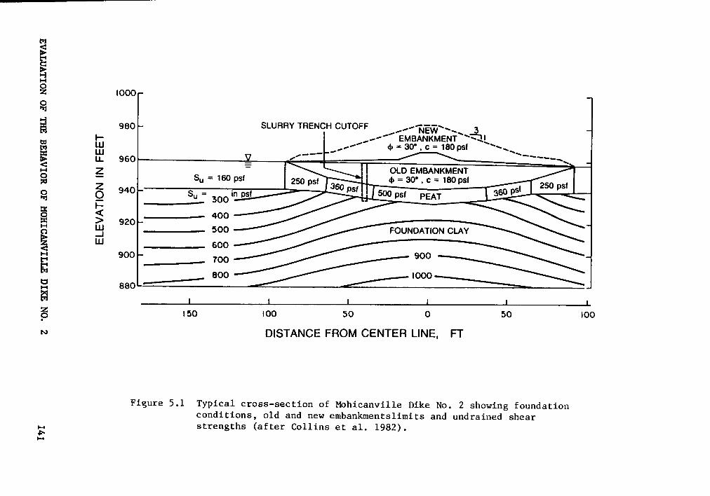
o—
9’
E{
2{
S[
Si;I
2%I,
Efä~·D
_*5,2
IL?E3
EI;
~§$5+
E"
'2Q
ufzä
'äzqm
qEd
E8
8°
Zgw
\§;2,5;%
2‘”
93
2:
\\u'*IIB
I!7*
DE
cu-EÄ
\Q
é°·
LIJ\°
8I-
•—+cnoo¤
“=Z
ԤԊ2ԥI.\
...3
22+
5JJ
OLL.
u-4rn
ZI
Lu°ä-E
EI
OS°„’3
I'\
Z··-+·+::o
>-\
<GGJ
In3
¤—
TBB
Ü:]9
Qgot;
IIIT5
8w
*V7
,Q
0::+
11
2.2
+-+-258
oo
oo
oo
mu
m..
oo
oo
oo
mu
¤
"IO
¢•D
IDN
=
"S
SS
°°r-I
IhOJ$4DBFoO
89
93
83
’“Q
0+0+
0+0+
0+aa
1.33:INI
NO
LLV/\3“|3
EVALUATIONOF
umBEHAVIOR
OFM
OHICANVILLEDIKE
NO.2
141
embankment. The limit equilibrium analyses were used to evaluate the
factor of safety with respect to shear failure through the embankment and
its foundation.
Because of the unusual design concept of the embankment and the im-
portance of the structure, a large number of instruments were installed
in the embankment and the foundation to confirm that the forces in the
reinforcement, the movements of the embankment, and the pore pressures
in the foundation were within acceptable limits during and following
construction. The information derived from these instrumentation studies
has been used to monitor construction progress and assess the accuracy
of the finite element analyses and stability analyses, as explained sub-
sequently.
Following construction, a second finite element analysis was per-·
formed, the results of which are reported herein. The purpose of this
new analysis was to more closely represent the actual field conditions
at the instrumented sections, including the strength of the reinforcement
as actually installed, and slightly different foundation and embankment
strengths than had been used in the original analyses performed by WES.
These changes were found to have only small effects on the calculated
results.
5.3 Review of Previous Studies
Previous studies on Mohicanville Dike No. 2 have been prepared by
Collins et al. (1982), Fowler et al. (1983) and Collins (1986). Collins
EVALUATION OF THE BEHAVIOR OF MOHICANVILLE DIKE NO. 2 142
et al. (1982) discussed the safety evaluation undertaken of the dike,
various alternatives for raising the dike, and made an analysis of the
use of reinforcement for raising the dike. They also presented a large
amount of data on the foundation conditions at the site, and the results
of a comprehensive laboratory testing program to characterize the foun-
dation and embankment soils. Fowler et al. (1983) performed finite ele-
ment analyses and stability analyses of the proposed design, and prepared
an instrumentation plan and cost estimates. Collins (1986) assembled,
reviewed and analyzed the instrumentation data collected during con-
struction of the dike.
Collins et al. (1982) proposed a procedure for determining the re-
inforcement required from limit equilibrium analysis of the form:
T = (MO [6.1]
where
T = required reinforcement force
FS = required factor of safety against failure
Mo = overturning moment due to embankment
bg.= resisting moment of the soil
R = radius of the critical slip circle.
Using this equation with the Law Engineering Testing Company (LETCO)
slope stability program (based on a "Modified Fellinius" or "Swedish"
method that satisfies moment equilibrium), the authors obtained the dis-
tribution of required reinforcement forces shown by the dashed line in
Figure 5.2. Their analyses were performed for an embankment height of
EVALUATION OF TIE BEHAVIOR OF MOHICANVILLE DIKE NO. 2 143
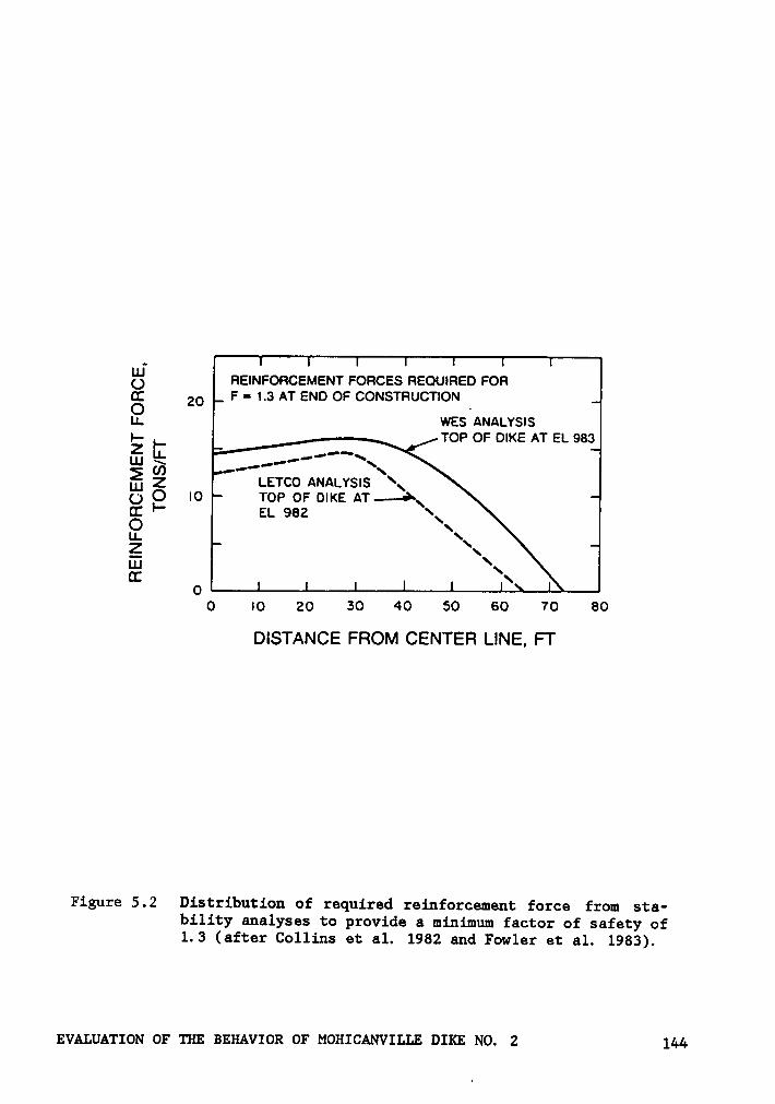
8 REINFORCEMENT FORCES REQUIRED FORE 20 F = 1.3 AT END OF CONSTRUCTION9. WES ANALYSISp- TOP OF DIKE AT EL 983E E
--···"“\cn
·"‘Z LETCO ANALYSIS
\\\
Q O IO TOP OF DIKE AT .-3~\¤: I- EL 982
\\E \\UJLI \x
00 IO 20 30 40 50 60 70 80
DISTANCE FROM CENTER LINE, FT
Figure 5.2 Distribution of required reinforcement force from sta-bility analyses to provide a minimum factor of safety of1.3 (after Collins et al. 1982 and Fowler et al. 1983).
EVALUATION OF ’TIE BEHAVIOR OF MOHICANVILLE DIKE NO. 2 144
22 feet, the design height at that time. It may be seen that these ana-
lyses showed that a reinforcing force of about 15 tons per foot would be
required to raise the factor of safety to a value of 1.3 at the end of
construction, as required by Corps of Engineers design standards.
A similar analysis was performed by Fowler et al. (1983) for an
embankment height of 23 feet, with the results shown by the solid line
in Figure 5.2. It may be seen that the results are very similar, the
maximum required force being about 1 ton/ft larger for the higher
embankment. Fowler et al. (1983) also examined safety with respect to
bearing capacity, lateral sliding, and splitting of the embankment, using
the procedures of Haliburton et al. (1982). The embankment was found to
be safe with respect to these other modes of failure as well.
A finite element analysis of the dike was performed by Fowler et al.
(1983) to investigate the influence of reinforcement stiffness on re-
inforcement force. This analysis will be referred to as the WES analysis.
The 1981 version of CON2D (Duncan et al. 1981) was modified to accommodate
reinforcing elements, and was used for the analyses. This program allows
consideration of consolidation effects and induced pore pressures, as
well as embankment deformations and reinforcement forces.
The analyses performed by WES used half sections of the embankment
and boundaries as followsz top of dike at elevation 983, working surface
at elevation 960, tce of dike at elevation 958 ninety feet from the
centerline, general ground surface at elevation 958, rigid base at ele-
vation 880 and no horizontal displacement at the centerline and 400 feet
from the center line. The steps of the WES analysis corresponded to crest
EVALUATION OF THE BEHAVIOR OF MOHICANVILLE DIKE NO. 2 145
elevations of 964, 970 and 978 during the first construction season,
consolidation during the winter, completion of the dike to elevation 983
in the spring, consolidation steps corresponding to two and eleven years
after the beginning of construction. The assumed cross section and
loading conditions differed somewhat from the actual construction se-
quence, as will be described subsequently.
For analyses using CONZD, soil strength, stiffness and permeability
properties are necessary. The values of these properties used in the WES
analyses were obtained primarily from the LETCO report (Collins et al.
1982) and were supplemented by limited testing performed by WES. The
model parameters were determined from laboratory tests following the
procedures described by Duncan et al. (1981) and D'0razio and Duncan
(1982). The soil strength values used in determining the initial soil
model parameters were the "design" strength values from composite en-
velopes wherein two-thirds of the test values exceed any design value,
as is standard Corps practice. Using these initial soil parameters, the
soil strength and stiffness properties were adjusted to match the labo-
ratory stress-strain curves. These computed curves were then "softened"
by reducing the soil strength and stiffness parameters such that a finite
element analysis of the unreinforced dike failed in correspondence to a
limit equilibrium of the unreinforced dike. In achieving these matches,
the strength values were reduced considerably from the initial values.
During the course of this study, computer code errors in the WES program
were discovered which may have influenced the selection of the model pa-
rameters.
EVALUATION OF THE BEHAVIOR OF MOHICANVILLE DIKE NO. 2 146
The reinforcement was modelled as elastic bar elements. Four values
of stiffness were used in the WES analyses: zero stiffness to represent
no reinforcement, 109 ton/ft to represent polyester fabrics, 625 ton/ft
to represent Kelvar products, and 12000 ton/ft to represent steel mesh
reinforcement.
From the analyses performed, the following conclusions were noted:
1. Lateral restraint of horizontal movement appeared to be the principal
mechanism through which load is transferred to the reinforcement,
2. The stiffer the reinforcement, the greater the load it carried.
3. The force in the reinforcement, the lateral spreading of the
embankment and foundation, and the pore pressures in the foundation
increased during embankment construction and decreased during subse-
quent consolidation periods.
4. Post-construction settlement was little affected by reinforcement
stiffness.
The relationship between mobilized reinforcement force and reinforcement
stiffness determined from the finite element analyses is shown in Figure
5.3. Also shown are the tensile strengths for various reinforcing mate-
rials. It is clear that only the steel reinforcing possesses the neces-
sary stiffness to achieve the working force as determined in the limit
equilibrium studies.
EVALUATION OF THE BEHAVIOR OF MOHICANVILLE DIKE NO. 2 147
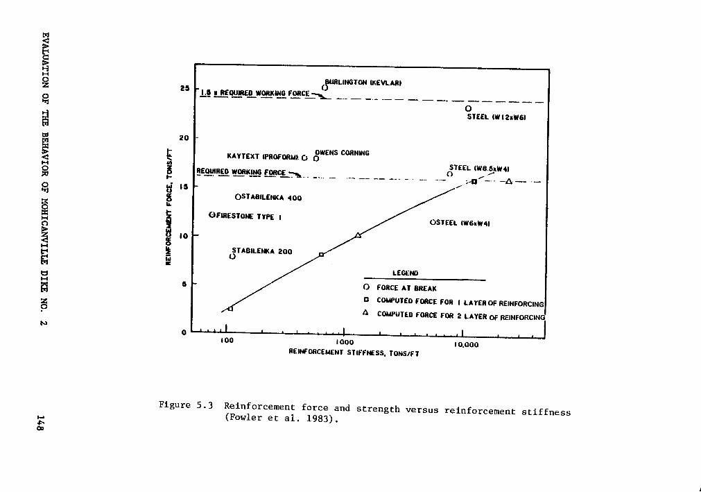
WW<III:U-4
oI
I2
2YS
I‘
°Q
"..
EW
GbI
oQ
IE
~2
2U
~;
QG
WC:
I;
='
ffE
EI
IIII
=C
EÜ
O¢F-‘
go
I;IO
};J
„ID
44
cQ3
I.I.I"-
BJ
·‘Q
I:I
·9I
3·
“9
*6"’¢
HI5
5=—·
II
u.u(D
IW
Ig
gIJ
I·
2°
“2
IZ¤>
·2
·:Q
I2Q
>az
I;
3„„
==
Q»=
4I
ggä
§•—
*53$J
I¤
°¢n°
I:“‘
II
“'Q
U(D
5·
.u
5'
2I
C°
"I:·
*6I-
IZ
IO
I:I
äI
S:
EJ
I—
Z¢¤
•U
)5
zI
·I;
^Q
rgW
_W
GJVÜ
°/
5gI
EE
äIJI
_¤
oI-I
sgI?
‘Q
2"‘
.IJ
=F
2Q
=·‘=‘1;:*,,
oIä
WI(
_2,
cuE
Q§‘
ä<
QI6,
§IE
•·-IEI
FE
U;
I_I:
5I-
InI·‘
Ix
2=.I4
2„_‘
<vQ
F§I
5Q
FSQ
gl4
3O
Ü:w
gQ
<II FnW
8Q
xa
TI2
‘~·2•
glQ
(7°I
,gl
I-O2
22
2·¤
¤§
I..·I1su¤1.'acsosm
snsasoaunauéc
EVALUATIO
NO
FT
IEBEH
AVIOR
OF
MO
IIICAN
VILLED
IKE
NO.2
148
Collins (1986) prepared a report summarizing and analyzing the
instrumentation data collected during construction of the dike. He con-
cluded that the embankment is stable and its construction was a success.
He also concluded that the finite element analyses were very valuable for
choosing the reinforcement type and for estimating the reinforcement
force, the pore pressures, and the deformations.
5.4 Properties of the Dike and Foundation.
The site is located on a glaciated plateau of the Killbuck Lobe of
Wisconsin age glacial deposits (White, 1967). This is a moraine belt of
upland glacial drift overlying bedrock with alluvium filled valley
floors. The topography of the area is bedrock controlled. The glacial
drift is a silty clay or "boulder clay," known as the Hayesville Till,
containing a wide range of particle sizes. The upland deposits of till
are from 3 to 12 feet thick. Kames and terraces are prevalent in the area,
having formed along the valley walls as glacial ice melted and receded.
The alluvial deposits, located in floodplains, are often thin, and
they overlie Hayesville Till deposits. The recent alluvium is generally
comprised of silts and sandy silts. The floodplains contain many
kettleholes formed during recession of the glaciers. These kettleholes
have filled with organic matter over the years to form peat and muck bogs.
The dike is located on a peat bog, with the peat overlying soft clay,
as shown in Figure 5.1. The foundation clay is very weak in the virgin
EVALUATION OF THE BEHAVIOR OF MOHICANVILLE DIKE NO. 2 149
state, because the low-weight peat deposits have not caused appreciable
consolidation to take place in the underlying clay.
A geotechnical investigation of the site was performed by Law Engi-
neering Testing Company (Collins et al. 1982). This investigation pro-
vides extensive information on the foundation conditions. Soil
properties of the foundation clay, peat, old embankment fill and borrow
areas were assessed through field vane shear tests and laboratory
triaxial, consolidation, permeability, compaction, and classification
tests (Collins et al. 1982). A summary of the test results is shown in
Table 5.1.
The foundation clay ranges in thickness from 10 to 60 ft and varies
across the site from a silty clay to an organic clay. The shear strength
of the clay where it has not been loaded by the old dike is very low, due
to the low unit weight of the overlying peat deposits. Typical undrained
shear strengths range from 300 to 1000 psf, as·shown in Figure 5.1.
Representative stress-strain characteristics of the clay as determined
from triaxial compression tests are shown in Figures 5.4 and 5.5, and
consolidation test results are shown in Figure 5.6.
The peat varies from fibrous near the ground surface to amorphous in
the lower portions of the deposit, and ranges in thickness from 16 feet
to 20 feet in the virgin state. Where it was compressed under the weight
of the old embankment, the thickness of the peat had been reduced to 11
to 15 ft. Typical undrained shear strengths for the peat ranged from
about 150 psf in the virgin state to about 500 psf where it had been
compressed under the old embankment, as shown in Figure 5.1. Stress-
EVALUATION OF THE BEHAVIOR OF MOHICANVILLE DIKE NO. 2 150
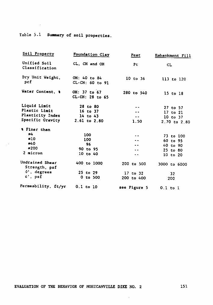
Table 5.1 Summary of soil properties.
Soil Property Foundation Clay Peat Embankment Fill
Unified Soil CL, CH and OH Pt CLClassification
Dry Unit Weight, OH: 40 to 84 10 to 36 113 to 120pcf CL·CH: 60 to 91
Water Content, S OH: 37 to 67 280 to 540 15 to 18CL·CH: 28 to 65
Liquid Limit 28 to 80 ·· 27 to 57Plastic Limit 16 to 37 -• 17 to 21Plasticity Index 14 to 43 —— 10 to 37Specific Gravity 2.61 to 2.80 1.50 2.70 to 2.80
S Finer than#4 100 —· 73 co 100#10 100 ·· 60 to 95#40 96 -- 40 co 90#200 90 co 95 -· 25 to 802 micron 10 to 40 ·· 10 to 20
Undrained Shear 400 to 1000 200 to 500 3000 to 6000Strength, psf¢', degrees 25 to 29 17 to 32 32c', psf 0 to 500 200 to 400 200
Permeabllity, ft/yr 0.1 to 10 see Figure 5 0.1 to 1
EVALUATION OF THE BEHAVIOR OF MOHICANVILLE DIKE NO. 2 151
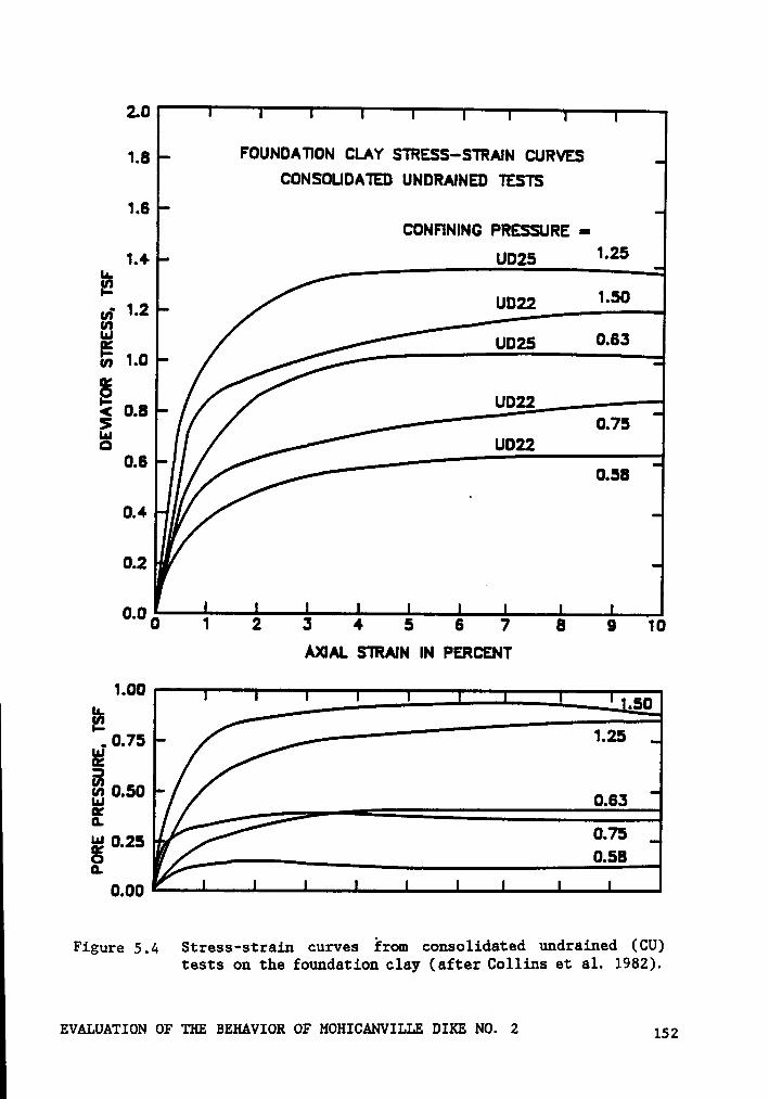
2.0
Lg FOUNDATION CLAY STRES$—STRA|N CURVESCONSOUDATED UNDRAINED TESTS
1.6CONFINING PRESSURE ¤
L4, UDZS 1.25LeI2U; 1.2IhE ums 0.63m 1.0
S’2¤.a
Suec0.6
°•4
'0.2 1I0.0 0 1 2 3 4 5 6 7 6 9 10
AXIAL STRAIN IN PERCENT
1 1.00
0.75u.:
ä 0.50tz0.ss
GL075W 0.25 1‘
0.00
Figure 5,4 Stress-strain curves from consolidated undrained (CU)tests on the foundation clay (after Collins et al. 1982).
EVALUATION OF THE BEHAVIOR OF MOHICANVILLE DIKE NO. 2 152

2.0
LB F0uNOA‘n0N CLAY STRESS—STRA|N CURVESUNCINSOUDATED UNDRAINED TESTS
1.6
1.4ttE· 1.233ue
1.0g CONFINING PRESSURE •I-< 0.8$ 2.25 TSF3
0.6
°·‘mum:
°°0012345678910Ax1AL STRAIN IN PERCENT
Figure 5.5 Stress-strain curves from unconsolidated undrained (UU)tests ou the foundation clay (after Collins et al. 1982).
EVALUATION or um azmvxox or uou1cANvu.r.¤ num No. 2 153
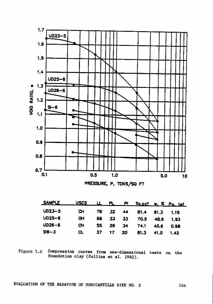
—!!IIIIII—IIIlII|I—ll!|IIII—IIIIIII|—lIIÜI"|—llIIIII|1.4 In
Z‘·"'
um-6 ‘··¤ ¤O __ ÄZ ¤lIl"'"$WIIIIIII—E=" “””¤M
InIn ‘IIIIII-|iiiir‘i*‘%
—!-.._-|||—L!IIIII|—IIIIII||—lllIII|I
0.1 0.5 1.0 5.0 10PRESSURE, P, TONS/SQ FT
§AMPL§ Q§Q§ |-L gl ßl 1‘g,gcf uv, X Eg, gggUD23-5 CH 76 32 44 61.4 61.3 1.19U025-6 OH 66 33 33 70.5 48.6 1.93UD26—6 CH 55 29 34 74.1 45.6 0.98S16-3 CL 37 17 20 81.3 41.0 1.42
Figure 5,5 Compression curves from one-dimensional tests on thefoundation clay (Collins et al. 1982).
EVALUATION OF THE BEHAVIOR OF MOHICANVILLE DIKE NO. 2 154

strain characteristics of the peat are shown in Figure 5.7, and consol-
idation characteristics are shown in Figure 5.8.
The permeability of the peat was assessed by performing field and
laboratory permeability tests. The results are compared in Figure 5.9
with values for California peats obtained by Weber (1969). It can be seen
that the Variations of permeability with consolidation pressure are very
similar for the California and the Mohicanville peats.
Both the old and the new embankment fill materials were derived from
glacial tills in the surrounding uplands. The fill material is a gravelly
sandy clay, with zones of gravelly clay. Pockets of poorly graded sand,
silt, silty sand and clayey gravel are also present in the borrow pit.
As it was compacted in the new embankment, the fill exhibits good shear
U strength characteristics, and is quite ductile at the in-place water
content of zero to two percent above optimum. The strength of the old
fill is somewhat lower, especially in areas where previous failures had
occurred.
The stress-strain and strength characteristics of the old and new fill
are shown in Figures 5.10 and 5.11. The tests on the new fill were per-
formed by the Huntington District on block samples taken from the
embankment after construction. It can be seen that the new fill exhibits
higher strength and modulus than the old fill. Consolidation character-
istics of the fill, determined from isotropic compression on a triaxial
test specimen, are shown in Figure 5.12.
EVALUATION OF THE BEHAVIOR OF MOHICANVILLE DIKE NO. 2 155
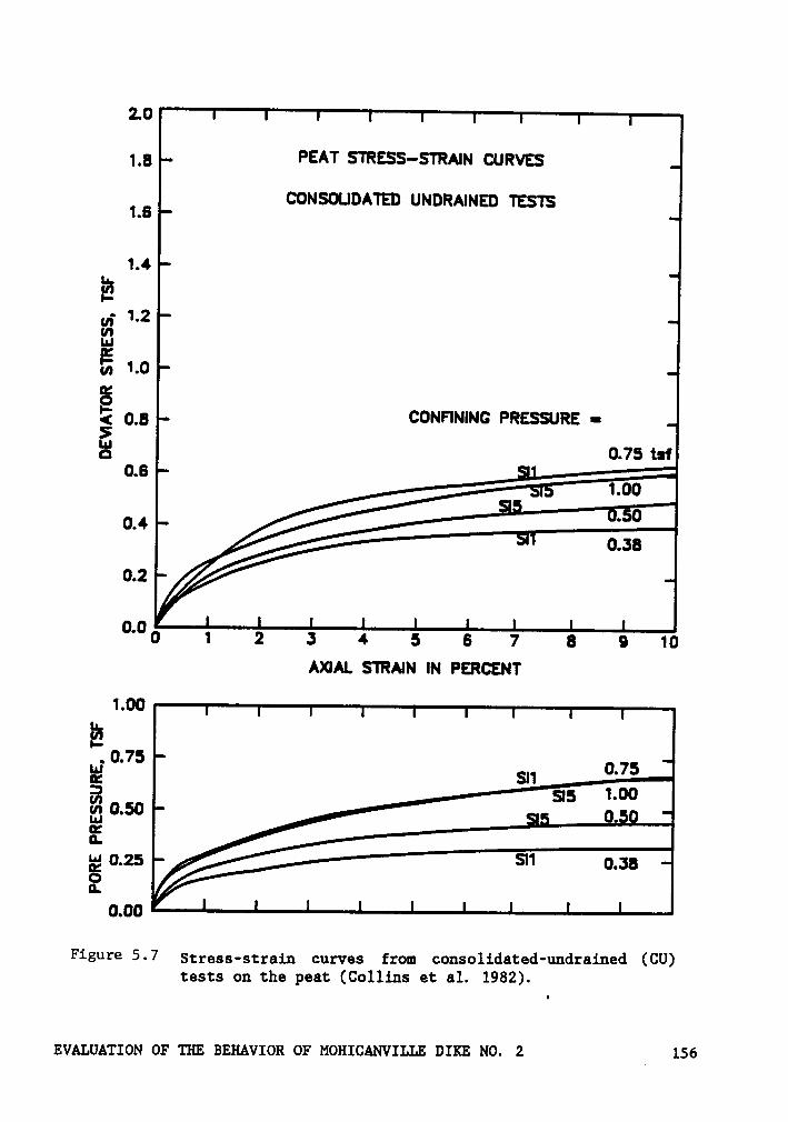
2.01_g PEAT STRESS-STRAIN CURVES
16 CONSOLIDATED uNORA1NE0 TESTS
1.4In-EV; 1.28
1.0§; M counnuuc Pnsssunc -S 0.75 es
0.6.0
° 0 1 2 J 4 5 6 7 0 0 10Axw. STRAIN um PERCENT
1.00
.0.75UM3 95 1.00
Ü.5Ü 1 0 ,M1
o1
0.00
Figure 5-7 Stress-strain curves from consolidated-undrained (CU)tests on the peat (Collins et al. 1982).
EVALUATION or ms azmvxox or MOHICANVILLE um: No. 2 156
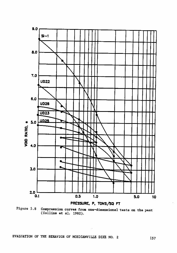
9.0
IIIIIIII—lIIIIIII
—l!IIIIII—IIIIIIII¤lllIIIII—IlIIIII|LIlIII|I|—IIIIIIII6.0 *.‘§!IIIII»I—IlIIIIII«·„UE!|II|IKIIIIIIIIQ 5-0,_„
—IIIIIIII—IIIIIII|0.1 0.5 1.0 5.0 10
PRESSURE, P, TONS/S0 FT l
Figure 5.8 Compression curves from one-dimensional tests on the peat(Collins et al. 1982).
EVALUATION OF 'TIE BEHAVIOR OF MOHICANVILLE DIKE NO. 2 157

,_ 30 • • CALIFORNIA PEAT E QI-IJ IZ 20 V •=n6¤.0 •<,., (gnuE-I- •AA LAB KV }D|KE NO. 2
¤0•j3 ¤ •°
0.5 w mA • • •ä Q• •
,_ m s •••• 0.2 äI•
Q E 2 . • • g 8]W ¤ 0.u I EI LU u_| U); ¤ > <„.. 2 no uoo I000 0 "
PERMEABILITY IN FEET PER HOUR x 10°5
Figure 5.9 Variation of peat permeability with height of fill,adapted from Weber (1969) and Collins et al. (1982).
EVALUATION OF THE BEHAVIOR 01·‘ MOHICANVILLE DIKE No. 2 158
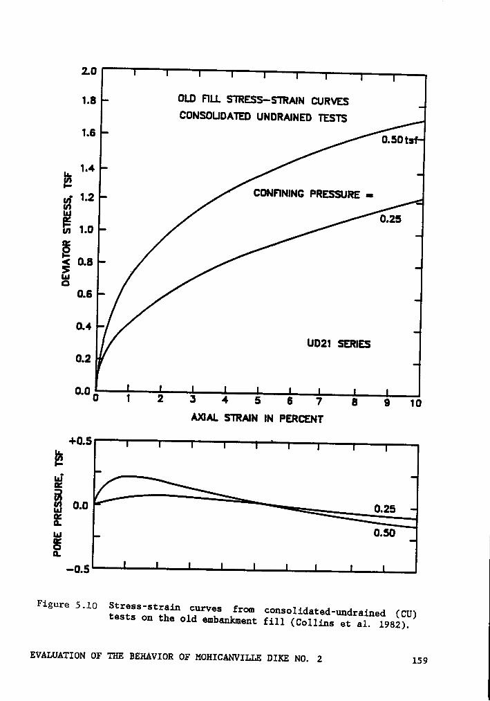
2.0
1.8 OLD FILL $TRESS—STRAIN CURVESCONSOUDATED UNDRAINED TESTS
1.80.50*l
184
E12 CONFINING PRESSURE ¤ _
g0.25
1.0
0.8g .Lu¤
0.8
0.4
UD21 SERIES
°'0OI234587891OAXIAL STRAIN IN PERCENT
+0.5
gQ
0.0I
E¤.
-0.5
Figure 5,10 Stress-strain curves from consolidated-undrained (CU)tests on the old embankment fill (Collins et al. 1982).
EVALUATION OF 'I'IE BEHAVIOR OF MOHICANVILLE DIKE NO. 2 159
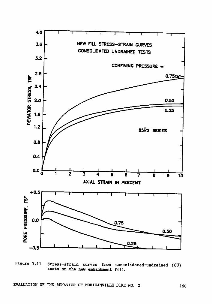
4.0
;_5 NEW FILL STRESS-STRAIN CURVESCONSOLIDATED UNDRAINED TESTS
3.2CONFINING PRESSURE ¤
k 2.8 0.75tsfI2
E 2.42.0
E 0.26°2 1.6E° -
‘·285R2 szmts
0.8
0.4V
°°0012345678910AXIAL STRAIN IN PERCENT
+0.5
IE Y0.0
EE *11.
-0.6 *6
Figure 5.ll Stress-strain curves from consolidated-undrained (CU)tests on the new embankment fill.
EVALUATION 01* THE BEHAV1012 or MOH1cANv1LLE DIKE No. 2 160
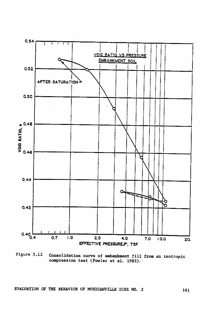
0.54 I I I I I I IVQIQ EAT|Q V§ EBEQQIRE‘
EMBANKMENT SOIL
0.52 1
I Il0.50 ‘*' I
·Q
"
I-<G
QO II‘|I|I
! L,. ulhi__
OIh
QIIIIIIIIII0.400.4 0.7 |.O 2.0 4.0 7.0 I 0.0 20.
EFFECTIVE PRESSURE„P°„ TSF
Figure 5-12 Cousolidatiou curve of embaukmaut fill from an isotropiccomprassiou test (Fowlar at al. 1983).
EVALUATION OF TIE BEHAVIOR OF MOHICANVILLE DIKE NO. 2 161
5.5 Properties of the Reinforcement
The stability analyses discussed previously indicated that a rein-
forcing force of about 15 tons per foot of embankment would be required
to raise the factor of safety to the required value of 1.3 at the end of
construction. The calculated distribution of reinforcing forces across
the embankment required for a factor of safety equal to 1.3 is shown in
Figure 5.2. The finite element analyses performed before construction
showed that a very stiff reinforcing material would be required to achieve
this amount of reinforcing force under working conditions.
To meet these requirements of stiffness and strength, a specially
fabricated steel mesh was used. The welded mesh consisted of #3 bars
spaced two inches apart along the length of the dike, with #2 bars six
inches apart parallel to the embankment axis. This mesh provides a the-
oretical ultimate reinforcement strength of 24 tons per foot of embankment
and a stiffness of 10,440 tons per foot of embankment.
The mesh was transported to the site in eight-foot wide rolls, and
was unrolled at the site using the same machine used to roll it in the
fabricating plant. When unrolled, the strips of mesh were cut into two
pieces, each eight feet wide and 160 feet long. These were dragged into
position on the embankment using a bulldozer. The reinforcement extended
80 feet upstream and downstream from the centerline of the embankment
between Stations 3+00 and 14+00.
The reinforcing mat was placed at elevation 960, approximately four
feet above original ground elevation. In most areas about six to eight
EVALUATION OF THE BEHAVIOR OF MOHICANVILLE DIKE NO. 2 162
feet of old fill had to be excavated to reach this elevation prior to
placement of the steel mesh. In one area where exceptionally large
settlements had occurred, additional fill had to be placed to raise the
surface elevation to 960 before the steel mesh was placed. A second layer
of reinforcing was placed at elevation 961 between Station 8+40 and Sta-
tion 9+40 as an added precaution, due to the uncertain foundation condi-
tions in this area. This was an area where extensive failure had occurred
in 1936 during original construction and a localized failure occurred in
1983 during construction of the slurry trench.
5.6 Field üeasurements
5.6.1 General
The dike, its foundation, and the reinforcement were instrumented
along four cross—sections as shown in Figure 5.13 and detailed in Table
5.2. A total of 39 piezometers of three different types were used to
measure foundation pore pressures. Thirteen inclinometers were installed
to measure movements of the embankment and the foundation. Nine of these
were vertical, and four were horizontal, placed just above the reinforcing
mesh to determine settlements at this elevation. Twelve settlement plates
were also installed to measure vertical movements near the reinforcement
level, and 25 surface monuments were installed to supplement the other
measurements.
EVALUATION OF THE BEHAVIOR OF MOHICANVILLE DIKE NO. 2 163
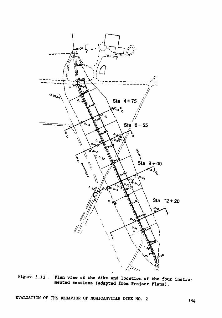
2_....1‘7’11 1 »—'=== “""
//1 ~\.__, 1'I IÜ
I 1; 11 x ./F··
FF \ ,'g 1?____°“" _ — _————______—_-_\/’_
FQo\ ‘ - \ /'!Os.) \ \ /1FMA: \ Sta 4+75 /1/
A. • 1’
x‘ °-1¤ \ ,9/
.- x "‘ \ 6' g_ff
\\\ °'?/ a° 1\\ \°—1" .· 11\1
e .2 x\\ 11 \ .,4Ä6 •'
, \\ _ 1 Sta 9+00
Ä v\/', \<•· Q'
-12
x1‘//„
2/_ \ Wqo \ Sta 12+20
F ‘~ F’1ß! _· \7_•°°
\ °-2 \1, \\1\ _ \ ‘„
¤' \„, / \ x\ \/’ •\F \<' F :·\ ;A· ••
1.\‘/1
\._ //1\ I
/1
Figure 5.l3‘. Plan view of the dike and location of the four instru-mented sections (adapted from Project Plans).
EVALUATION OF THE BEHAVIOR OF MOHICANVILLE DIKE NO. 2 164
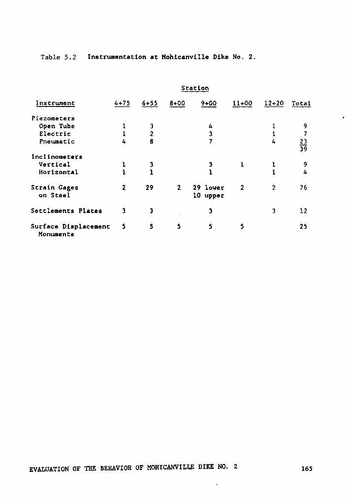
Table 5.2 Instrumentation at Hohicanville Dike No. 2.
Station
Instrument 4+75 6+55 8+00 9+00 11+00 12+20 TotalPiezometers 'Open Tube l 3 4 1 9Electric l 2 3 l 7Pneumatic 4 8 7 4 2339Inclinometers
Vertical 1 3 3 1 1 9Horizontal 1 l l 1 4Strain Gages 2 29 2 29 lower 2 2 76on Steel
10 upper
Settlements Plates 3 3 A 3 3 12Surface Displacement 5 S S 5 5 25Honuments
EVALUATION OF THE BEHAVIOR OF MOHICANVILLE DIKE NO. 2 165

Strain gages on the reinforcement provided a direct means of deter-
mining the force in the steel reinforcement throughout construction. Of
76 strain gages installed on the reinforcing mesh, only two have failed
to provide continuous readings, and the data appear to be very consistent
and reliable.
A plan view of the project showing the dike and the location of the
instrumented sections is shown in Figure 5.13. Cross·sections of the
instrumented sections showing the ground surface profile and foundation
conditions prior to reconstruction, are shown in Figures 5.14 through
5.17.
As may be seen from Figures 5.14 and 5.17, at Stations 4+75 and 12+20,
the thickness of soft clay is about 13 feet and the thickness of peat
ranges from 10 to 19 feet in the virgin state to seven to nine feet where
the old embankment compressed the peat. The peat on the upstream side
appears to be thicker than on the downstream. The thickness of the peat
and clay is on the order of 20 to 30 feet at these sections with a firm
layer at around elevation 930. Because the weak strata at these stations
are thinner, higher factors of safety and smaller movements would be ex-
pected than at Stations 6+55 and 9+00, where the thickness of weak foun-
dation materials is on the order of 60 feet.
Figures 5.15 and 5.16 show the foundation conditions at Stations 6+55
and 9+00. At these stations, the thickness of the peat is similar to that
at Stations 4+75 and 12+20. At Station 9+00 a discontinuity of the peat
is shown reflecting the previous shear failures that took place in the
EVALUATION OF THE BEHAVIOR OF MOHICANVILLE DIKE NO. 2 166
1
I
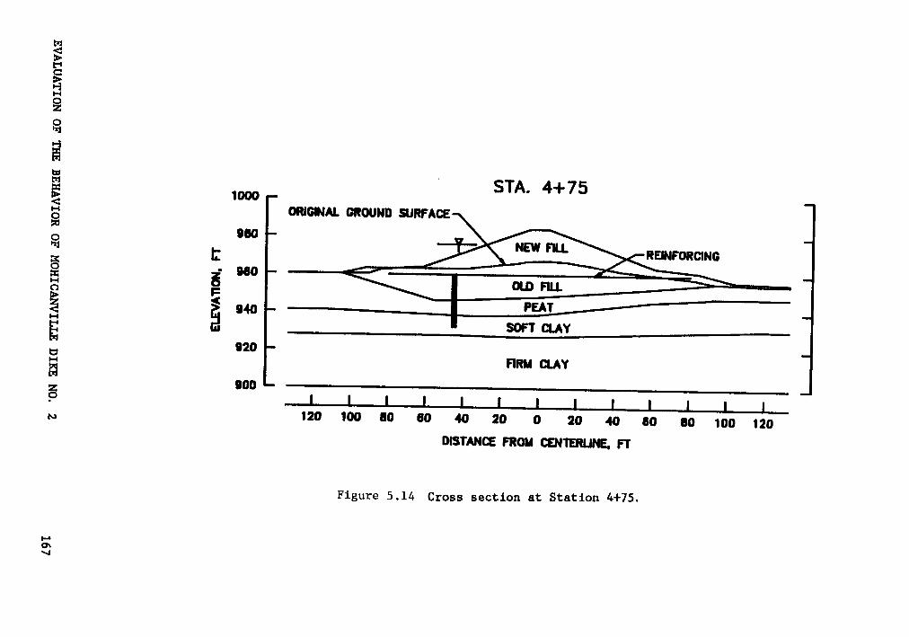
{
°—
*200Q
F
ä—
S2E
21
2F
§:1an
„ä
3IN
>_ea
gf+
"··
<-5
EÄ
°Ü
jf‘
‘*2
ä°°
<c:
•·E
„E
25
3·
$E
22
B°
2E
¤°
ä°
2•—«
0Q
LAä
25
§gg
ää0
EE
00
0ä
E2
E2
21.1
°N0|.I.VA313
EVALUATION
OF‘I'I·E
BEHAVIOROF
MO
HICANVILLED
IKENO.
2167
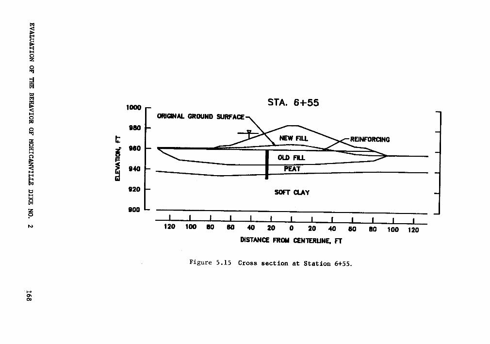
oE!oU
Eägg
Sä
caZ
gug
EÜ?»¤
$IJ
Q
=3
|-Oas
**-2>·
5,*co
ää
-°
ää
·S
ä2
ä«»“2:
2W.
9:7,
···2
2E
3E
,3
28
«„;oa
EÜ
3E
1*zc
‘Ü
_¤
cc
_§E
2E
22
.u‘uou.vAa1a
EV
ALU
ATIO
NO
FTH
EB
EH
AV
IOR
OF
MO
HIC
AN
VILLE
DIK
EN
O.
2153
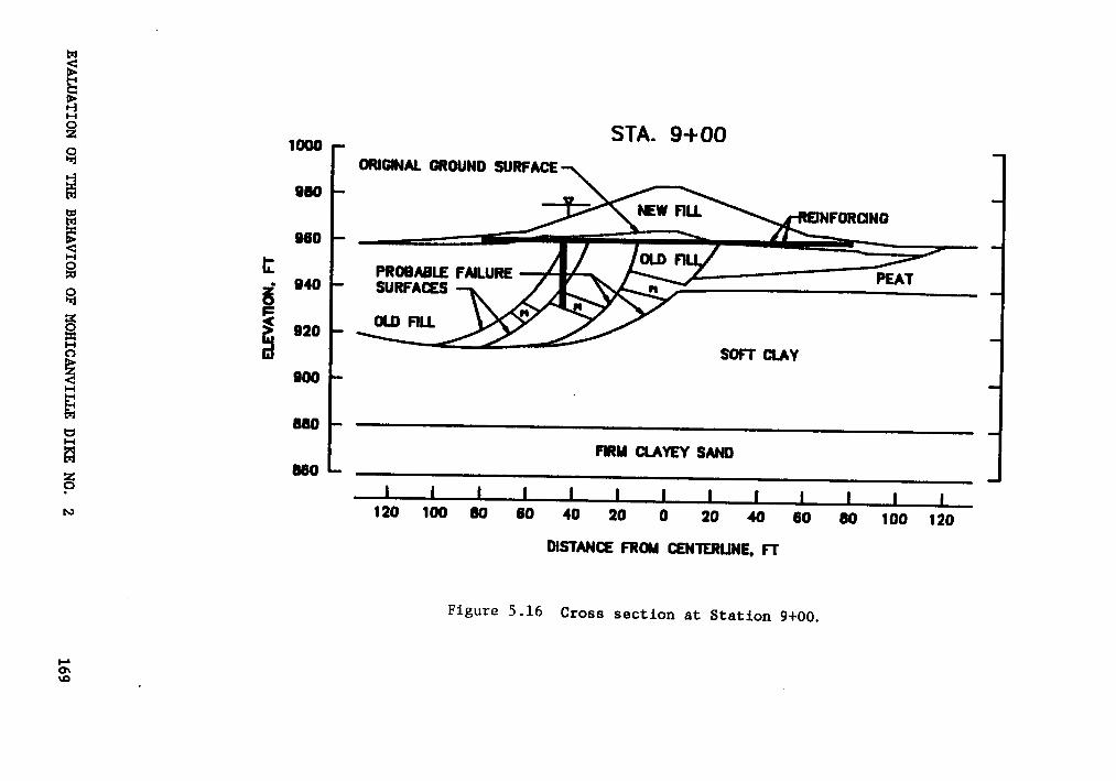
";
25
EOD
”"5
nr:
ÄO
2„,
*O
Inc2
ä"
E2
°*E
2”
2.
¢8
gg
5{
2E
„2.0
22
gÜ
Y
äc
2*
°T.?
2,E
3g
25
E5
32
E252
*E
Q5
55
55
55
.IJ°PDlI.W
\3"I3
EV
ALU
ATIO
NO
F'T
IEB
EH
AV
IOR
OF
MO
HIC
AN
VILLE
DIK
EN
O.
2169
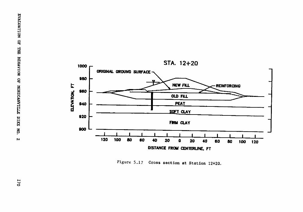
ß252
F_§
25
.nz
~
2E
i¤
5+
,>·
>-N
W
,9*E
33
°5
5.
¤-g
5<
TJI-
¤g
UI
N8
vzU)
.2
§8
=°
E3
:E
:Z
S*—•
32
E2
°E
2=
IZ
¤
52
¤..1—1..1_.1._«¢
Q_§
22
E2
§J.-!
°NO
ILVA3'I3
EV
ALU
ATIO
NO
FTH
EB
EH
AV
IOR
OF
MO
HIC
AN
VILLE
DIK
EN
O.
2170
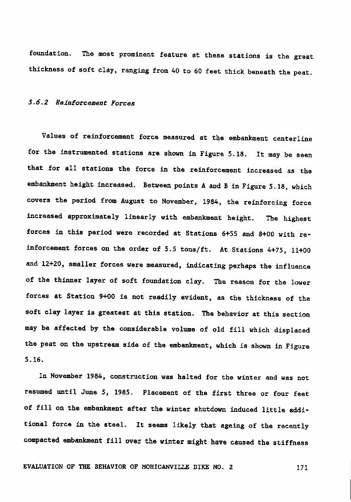
foundation. The most prominent feature at these stations is the great
thickness of soft clay, ranging from 40 to 60 feet thick beneath the peat.
5.6.2 Reinforcement Forces
Values of reinforcement force measured at the embankment centerlinefor the instrumented stations are shown in Figure 5.18. It may be seen
that for all stations the force in the reinforcement increased as theembankment height increased. Between points A and B in Figure 5.18, which
covers the period from August to November, 1984, the reinforcing force
increased approximately linearly with embankment height. The highest
forces in this period were recorded at Stations 6+55 and 8+00 with re-
inforcement forces on the order of 5.5 tons/ft. At Stations 4+75, 11+00
and 12+20, smaller forces were measured, indicating perhaps the influence
of the thinner layer of soft foundation clay. The reason for the lower
forces at Station 9+00 is not readily evident, as the thickness of the
soft clay layer is greatest at this station. The behavior at this section
may be affected by the considerable volume of old fill which displaced
the peat on the upstream side of the embankment, which is shown in Figure
5.16.
In November 1984, construction was halted for the winter and was not
resumed until June 5, 1985. Placement of the first three or four feetof fill on the embankment after the winter shutdown induced little addi-
tional force in the steel. It seems likely that ageing of the recently
compacted embankment fill over the winter might have caused the stiffness 4
EVALUATION OF '1'IE BEHAVIOR OF MOHICANVILLE DIKE NO. 2 171
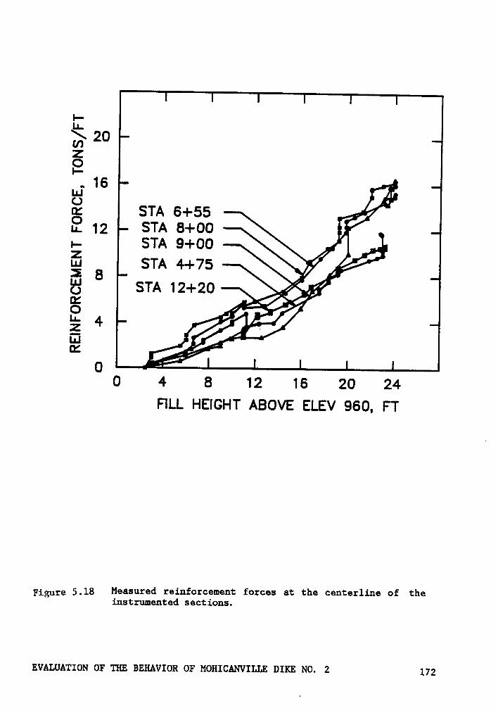
'Liä 20äH
16Llj
l'
ä STA6+55LL12 STA 8+00 fl
Ii STA 9+00 .ä 8 STA 4+75 ,6/
I ,·'STA 12+20 L
’/g __;@’°
*64zEMZ06/
0 4 8 12 16 20 24FILL HEIGHT ABOVE ELEV 960, FT
Figure 5.18 Measured reinforcement forces at the centerline of theinstrumented sections.
EVALUATION or um BEHAVIOR or M01ucANvu.L6 num No. 2 172
cf the fill to increase sufficiently to affect its interaction with the
reinforcement and the foundation. This possibility was investigated
through laboratory tests and finite element analysis and will be discussed
subsequently. As further fill was placed on the embankment, above about
14 feet, the rate of increase of reinforcing force returned to that prior
to the winter shutdown.
An interesting phenomenon is indicated by the data at point C in
Figure 5.18. At a constant embankment height (approximately 19 to 20
feet) the reinforcement force increased by about two tons per foot over
a period of nine days. The increase in force at Stations 4+75 and 12+20
was less than a half of a ton per foot, indicating the increase is most
likely an effect of the thickness of the soft clay layer. This increase
in force is thought to be due to undrained creep in the foundation soils,
primarily the clay.
The centerline reinforcement force at all the stations initially in-
creased after the end of construction. At Stations 8+00 and 9+00 the
force began to decrease within one to two months after construction.
Small increases of less than one-half of a ton per foot occurred at
Stations 6+55, 11+00 and 12+20 during the period from August, 1985 to
March, 1986. At Station 4+75 the force has increased nearly two tons/ft
during the same period, despite a significant drop in pore pressure at
this station.A
Between Stations 8+40 and 9+40 two layers of reinforcement were used,
spaced one foot apart vertically. This area is where the worst failures
had occurred during construction of the original embankment, where a
EVALUATION OF THE BEHAVIOR OF MOHICANVILLE DIKE NO. 2 173
failure of the side wall of the slurry cutoff trench occurred during its
construction, and where the foundation conditions are most uncertain. A
number of points of interest can be noted from the measurements of rein-
forcing force made in this area, which are shown in Figure 5.19: First,
the lower layer of steel carries considerably greater force than the upper
layer, although both have the same properties. Second, the fraction of
the total reinforcement force provided by the lower layer increases with
increasing embankment height. Third, after construction of the
embankment was completed (Point D in Figure 5.19), the force in the lower
layer of steel mesh increased slightly while the force in the upper layer
decreased by about 50%. Although many factors may be involved in this
complex behavior, the most important factor appears to be that the ef-
fectiveness of embankment reinforcement is improved by placing it lower
within the embankment, and the lower layer of steel mesh is thus in a
position to be more effective than the upper layer.
Distributions of the reinforcement forces across the embankment at
Station 6+55 are shown in Figure 5.20 for various times during con-
struction. Throughout construction the maximum force occurs at the center
of the embankment, as would be expected. In the downstream portion of
the embankment the variations of force with distance from the centerline
are smooth and regular, indicating that the measurements probably contain
little scatter. In the upstream portion of the embankment the re-
inforcement forces are more erratic, and are believed to be influenced
by the slurry trench cutoff wall, which was located 45 feet upstream from
the centerline. As the embankment height increases above 16 feet, the
EVALUATION OF THE BEHAVIOR OF MOHICANVILLE DIKE NO. 2 174
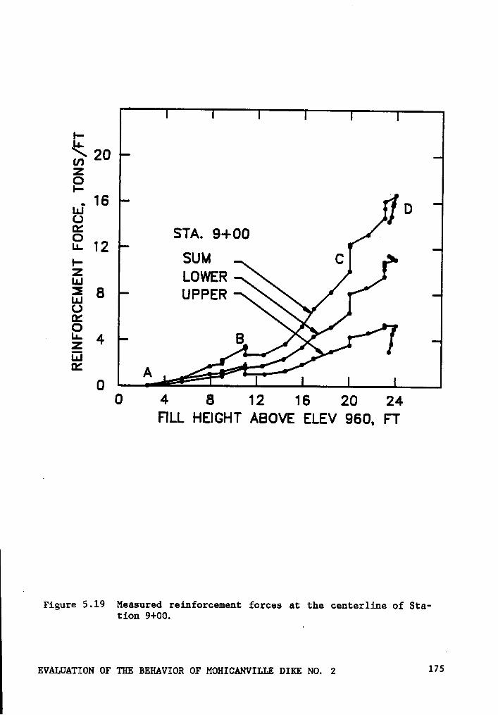
Eg 20ZOI- .LJ 16 D0g sm. 9+00 Iu. 12,. SUM CE LOWER
8 UPPERU
äÜ j
A_- g
0 4 8 12 16 20 24FILL HEIGHT ABOVE ELEV 960, FT
IFigure 5.19 Measured reinforcement forces et the ceuterliue of Sta-
tion 9+00.
EvAL¤A1*10N 01·* um Bmmvxox or M0u1cAuv11.LE 0110; No. 2 175
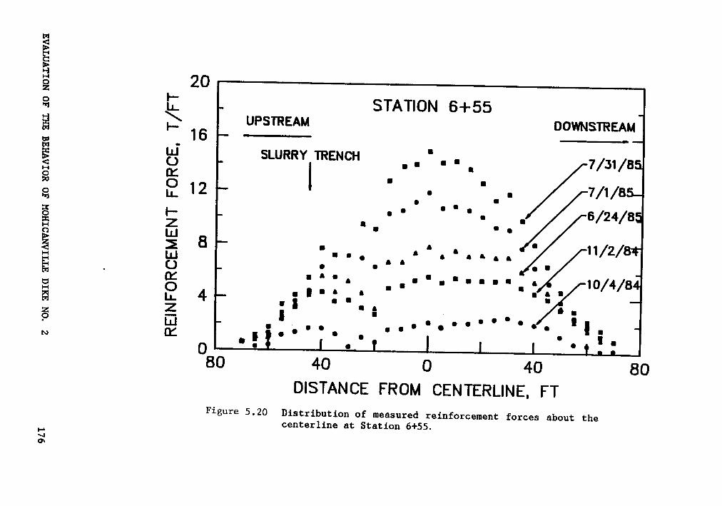
„O
.Q
-
¤¤Q
QM
6>
:3~
~*·
E\
\x
·•·,,,
ä
Ä"
ID1
-•-
•-E
I1
I
IQ
•I_
L;
III
•L
LO
I•
•I
•3
gI
QL
L;
U
II
4I
Q,
ZI
II
IQ
Ja
tgI
••
I•
&Q
+
ÜI
II
I[Q
§
(DI
•I
I•
ZO
II
I|
‘•
LU
Z
II
QU
Q-
OI
Iu
m
;I
IQ
.•ff
'.1
11
·3
2'
u.3II
(flI
•«
a«
LIJJJ
II
II
I·•-I
0E
lI
I(
II
O|E
u:—
I_
It
$.4Q<
Q;
••••
ÜÜ
Üg
,,,,
38(IJ
ä'
ca¤-
n°f
DIh
Qos
Oco
N¤¤
<-¤°°
“N
Y'-
Y1
.L:|/.L'EO
HO
JLNHW
BOHO
.-INIBH
EVALUATIONOF
THEBEHAVIOR
OFMOHICANVILLE
DIKENO.
2176
reinforcement forces continued to increase at the centerline, but did not
increase much beyond about 40 ft from the centerline. Measurements of
reinforcement force since the end of construction (see Table A-4 in Ap-
pendix A) show that the forces are still increasing near the centerline,
although the March 1986 values show only slight increases over the De-
cember 1985 values. In the upstream portion the forces increased after
end of construction and in the downstream portion the forces decreased
after construction. Whether this difference is due to the presence of
the slurry trench or to differences in stratigraphy is uncertain.
The distribution of reinforcement forces about the centerline at
Station 9+00 also reveal some interesting tendencies. The data for Sta-
tion 9+00 is tabulated in Table A-5 in Appendix A. It may be seen that
while the lower steel takes the larger share of the load near the
centerline as noted in Figure 5.19, near the upstream toe the upper steel
takes about twice as much load as the lower steel. The trend quickly
reverses itself near the slurry trench. Unfortunately, no strain gages
were placed on the upper steel near the downstream toe, so it is not
possible to determine if the upper steel near the downstream toe is also
carrying a higher force. The data does show that the lower steel on the
downstream side carries higher and more uniform forces. The Variations
in force in the lower steel follow the pattern noted above for Station
6+55, namely that the downstream Variation is smooth and regular while
the Variation upstream is erratic, particularly near the slurry trench.
EVALUATION OF THE BEHAVIOR OF MOHICANVILLE DIKE NO. 2 177
5.6.3 Pora Pressures
Values of pore pressure measured during and after construction are
shown in Figures 5.21 through 5.27. Figure 5.21 shows pore pressure
values as a function of fill height for piezometers located in the peat
near the centerline of the four instrumented sections. Figure 5.22 shows
a similar relationship for the foundation clay. The pore pressures in
the peat at Stations 4+75 and 6+55 rise at a rate slightly greater than
one foot of head per foot of fill. Because the unit weight of the
embankment fill was about 136 lb/ft’, one foot of increase in pore pres-
sure per foot of embankment height would correspond to pore pressure ratio
value of ru = 62.4/136 = 0.46. The pore pressures measured in the peat
at Stations 9+00 and 12+20 rise at a somewhat lower rate. The rate of
rise of the crest elevation at the four instrumented stations versus time
was very similar, from which it is concluded that the rate of load ap-
plication for the four sections was also very similar. Thus the differ-
ence in pore pressure rise is probably due to differences in the drainage
conditions and permeability of the peat at each station.
A somewhat different picture emerges when pore pressure levels in the
foundation clay are considered. As shown in Figure 5.22, the pore pres-
sures in the clay at Station 8+95 are quite high and have been high since
early in construction. The pore pressures at Station 6+52 show about a
1:1 rise with embankment height but remain below the mark of piezometric
head equalling embankment elevation. Collins (1986) attributed the low
pore pressure in the foundation clay at this station to a faulty seal in
EVALUATION OF THE BEHAVIOR OF MOHICANVILLE DIKE NO. 2 178
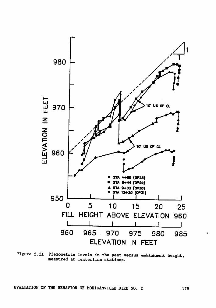
I11980 ,//
//1 /’/1
1,. ,4 / //E 970 1o* us 6: ¤_
z ‘
,21/ f 10* us or CL
> 1LAJ 960..ILU
• :1*4 6+60 (01•26)u STA 6+64 (¤P2•)4 STA 9+03 (van)•
STA 12+20 (¤1•:11)950
0 5 10 15 20 25FILL HEIGHT ABOVE ELEVATION 960
960 965 6 970 975 980 985 'ELEVATION IN FEET
Figure 5.21 Piezometric levels in the peat versus embankment height,measured at cexxterliue stations.
EVALUATION OF THE BEHAVIOR OF MOHICANVILLE DIKE NO. 2 179
I
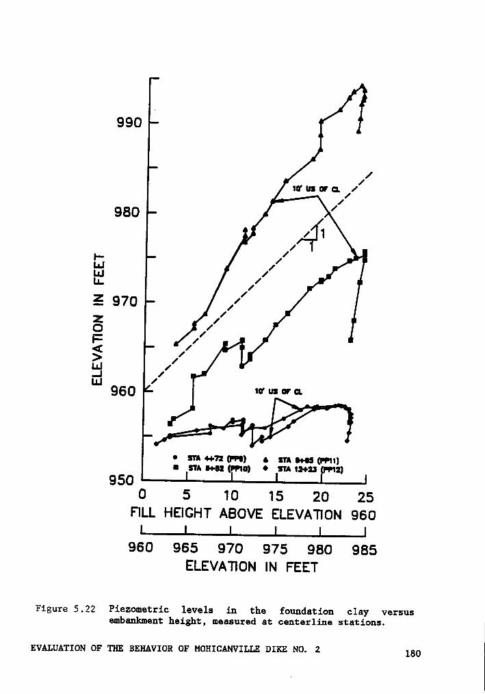
990I
/10* us 0r ¤. /1/
/1980
11|111I: 1E ,1/
E 970,/’
ä 1/E //ä
1’Ü
//ggg 10* us 0r 1:.
• true-•-12(FP9) •STAB-I5(91|)l sm 0+02 (H10) • $1012-•·2:a•r12)
9500 5 10 15 20 25
FILL HEIGHT ABOVE ELEVATION 960
960 965 970 975 980 985ELEVATION IN FEET
Figure 5.22 Piezometric levels in the foundation clay versusembaukmeut height, measured at ceuterline stations.
EVALUATION OF THE BEHAVIOR OF MOHICANVILLE DIKE NO. 2 180
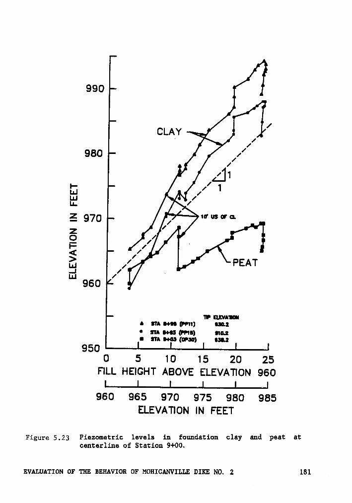
990
cI.Av’
960„“
1L3, /
E 970 1¤*us¤=¤.
ä /F // '< //5 ,/ PEAT.I / ILu /
960
1u•¤.£vA‘n¤••• s1A•+••(r••11) un.:•S'I’AI·•-ISOPIS) no.:•STA!-+03(03¤) Ill.!
9500 5 10 15 20 25
F'ILL HEIGHT ABOVE ELEVATION 960
960 965 970 975 980 985ELEVATION IN FEET
Figure 5.23 Piezometric levels in foundation clay and peat atcenterline of Station 9+00.
EVALUATION OF TIE BEIIAVIOR OF MOHICANVILLE DIE NO. 2 181 7
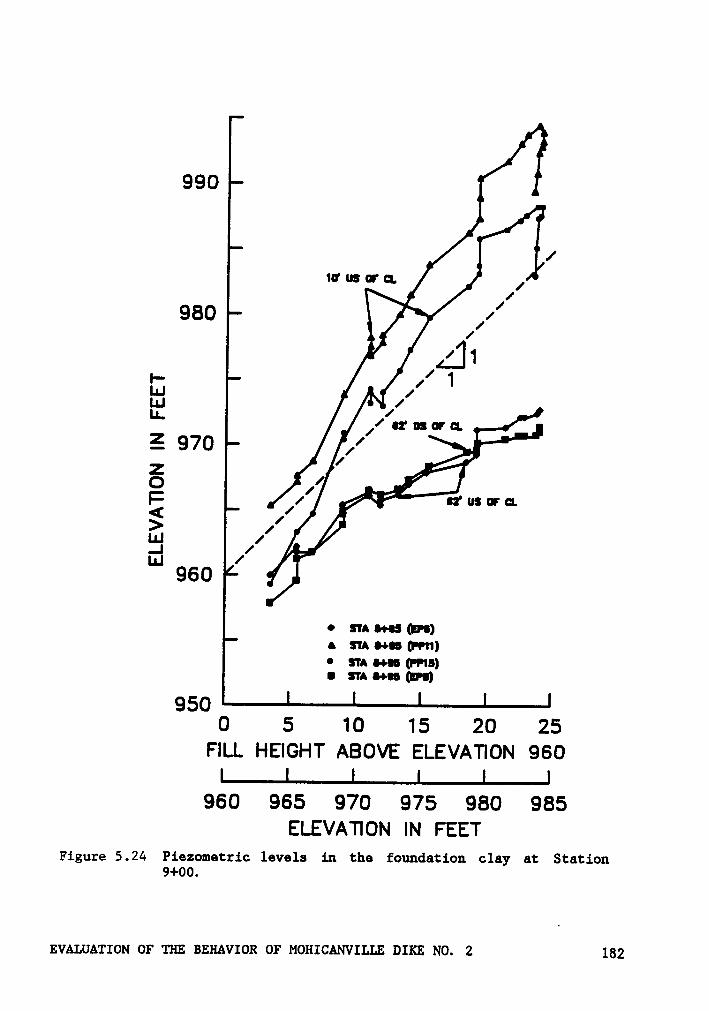
990
/1U us er ¤. //1
980 /11
411E ILuU"
// •z' user erE 970 /Z 1Q 1I: 1/ •2‘ us er eu.( /> /u.I 1Ü
//
960
• STA|+l5(DI)A STA
•+•S(P11)• s·rA•+•¤u•r1s)
•STA
•+•s(De)
9500 5 10 15 20 25
FILL HEIGHT ABOVE ELEVATION 960
960 965 970 975 980 985ELEVATION IN FEET
Figure 5.24 Piezometric levels :Ln the foundation clay at Station9+00.
EVALUATION OF THE BEHAVIOR OF MOHICANVILLE DIKE NO. 2 132
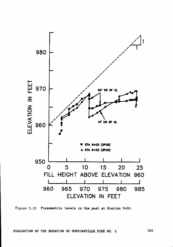
1/ I1
1 1980/1
/11/1
1/1I- //IL1 970/
Z 1///
// 10° US G 0LI-LI J
l STA 9+03 (G3!]• sm uns (wan)
~ 9500 5 10 15 20 25
FILL HEIGHT ABOVE ELEVATION 960
960 965 970 975 980 985ELEVATION IN FEET
Figure 5.25 Piezometric levels in the peat at Station 9+00.
EVALUATION OF 'TIE BEHAVIOR OF MOHICANVILLE DIE NO. 2 183
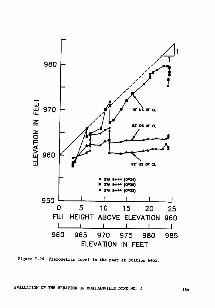
// I1
1 1980 ,/1
1/11/1
g- 1
Ü 10‘ US G Q1
sz' os or cn.Z 1ng //
un 960 F—| .LU S2' US OF CL
• STA •-+44 (W34)n STA 0+44 (N2!)•
STA S-•·44 (OPS:)
9500 5 10 15 20 25
FILL HEIGHT ABOVE ELEVATION 960
960 965 970 975 980 985ELEVATION IN FEET
Figure 5.26 Piezometric level in the peat at Station 6+55.
EVALUATION OF 'l'HE BEHAVIOR OF MOHICANVILLE DIE NO. 2 134
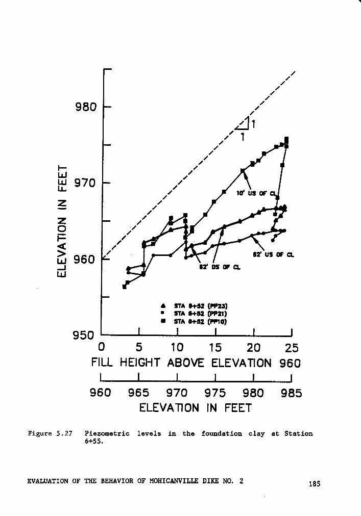
/1/1
/1980 /1/
A111 1 „/1
/1E /L1-E 970 /,1 —
1
z 19 1’ 1·‘ff
ÄJ S2' US Gd._; •2'
us G CLLIJ
•s1*n•+s2(rP2a)•STA I+S2 (PPZI)•sm 84-52(PP10)
9500 5 10 15 20 25
FILL HEIGHT ABOVE ELEVATION 960
960 965 970 975 980 985ELEVATION IN FEET
Figure 5.27 Piezometric levels in the foundation clay at Station6+55.
EVALUATION OF THE BEHAVIOR OF MOHICANVILLE DIKE NO. 2 185
the piezometer, allowing pore pressures to dissipate, and believed that
the actual pore pressures probably approach those at Station 9+00. The
piezometric level in the clay at Stations 4+75 and 12+29 show little re-
sponse to the embankment loading.
The piezometric levels under the centerline near Station 9+00 for the
peat and clay have been plotted in Figure 5.23 for ease of comparison.
It may be seen that the head in the clay increased at a rate that is higher
than 1:1 with embankment elevation, indicating the value of qlis larger
than 0.46. This is in contrast to the pore pressures measured in the peat
which plot below the 1:1 line. A distance of only about eight feet ver-
tically separates the tips of the two piezometers. The piezometer showing
the high pore pressure levels are likely located in or near a previous
failure zone in the foundation clay, as may be seen from Figure 5.16.
Conditions here may be such that the prior failures have resulted in high
shear stresses in the clay, such that when additional loads are imposed
on the soil, corresponding higher pore pressures result. Despite these
high pore pressures, the highest reinforcement forces were not measured
at this station. This may be a consequence of the large volume of old
fill upstream providing support to the new fill.
In Figure 5.24 the piezometric levels in the clay upstream, downstream
and near the centerline are plotted versus embankment height. It may be
seen that the pore pressures at the centerline are higher than at the
toes, even at low fill heights when the induced loads would be of compa-
rable magnitude. This is in contrast to the behavior in the peat shown
in Figure 5.25, where at low fill heights the response at the center line
EVALUATION OF THE BEHAVIOR OF MOHICANVILLE DIKE NO. 2 186
and downstream was nearly the same. Thus, much higher pore pressure re-
sponse in the foundation clay at the centerline is most likely a result
of the effects on the soil of the previous failures.
During the winter shutdown, piezometric levels in the peat declined
considerably, while those in the foundation clay declined only slightly.
In the peat, loading during the second construction season induced much
more pore pressure near the centerline than at the toe, as would be ex-
pected. In the foundation clay, the pore pressure at the toes increased
much more than in the peat, indicating greater load was being transferred
to these areas, or slower drainage, or both. The pore pressures in the
clay and peat at the centerline have been decreasing since the end-of-
construction while those at the toes have increased slightly. This is
believed to be due to dissipation of the pore pressures accompanied by
drainage outward from the centerline to the toe areas.
Piezometric levels in the peat and clay at Station 6+55 are shown in
Figures 5.26 and 5.27. It may be seen that the pore pressures near the
toes in the peat increased with embankment loading through the first
construction season, dissipated during the winter shutdown and then in-
creased slightly during the second construction season. The embankment
level above these piezometers was about 964 feet at the end of con-
struction. A similar pattern exists for the piezometric levels in the
foundation clay. The pore pressures in the clay during the second con-
struction season rose more than those in the peat, which may be due to
the lower permeability of the clay. The lower pore pressures experienced
· upstream may be due to the greater thickness of old fill upstream.
EVALUATION OF THE BEHAVIOR OF MOHICANVILLE DIKE NO. 2 187

In both the peat and the clay, the increase in pore pressure is greater
beneath the center of the embankment than upstream and downstream. In
both the peat and the clay at Station 6+55, the response for piezometers
downstream from the center is slightly greater than for piezometers the
same distance upstream. In addition, at both Stations 6+55 and 9+00 the
pore pressures continued to increase in the downstream peat after con-
struction. It seems likely that this was due to the effect of the slurry
trench cutoff, restricting drainage of the foundation soils. The cutoff
is located 45 feet upstream from the embankment centerline, and probably
restricts lateral migration of high pore pressures from the center of the
embankment in the upstream direction.
5.6.4 Settlements and Horizontal Hovemsnts
Settlements measured using horizontal inclinometers located at the
four instrumented station are shown in Figures 5.28 through 5.31. The
measured settlements at Station 4+75 and 12+00 (Figures 5.28 and 5.31)
were greatest at the centerline, with a small amount of heave occurring
near the downstream toe within eight months after construction. The
maximum settlements were about 0.4 feet at the embankment centerline at
the end of construction (July 1985), and approximately 0.1 feet of addi-
tional settlement occurred within eight months after construction.
The settlement at Station 9+00 (Figure 5.30) was the highest recorded,
with settlements of nearly one foot occurring by the end_of construction
and of one and one half feet by March, 1986. Rather uniform settlement
EVALUATION OF THE BEHAVIOR OF MOHICANVILLE DIKE NO. 2 188
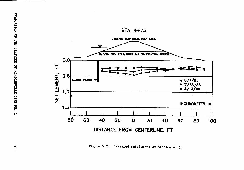
02
EID
Ql'
llÜ
tnU
QU-|
O
IlSEE
Mä
°°I
\\\
j‘
uar~
nQ
II
(I
;é
I-3;
I1Q
L"
-5<1·
·Q
IIä
Qu
Z+·
3Q
ME
NLU
:1=¤
E5
‘“3
[\2
Z'2
J;Q
EÜ
1:O
3E
esÜ
äo
flU')
'SÜ
:·.¤
Eo
'-'·Q
Qä
Nu.•
3'~
0Zoo
S'
OF
E•¢
Q11.E
goco
>
Q¤¤
°°.I..·.|
°.I.N3N3”LL.L3S
EVALUATIONOF*1*111:Bmmvxox
01*MOHICANVILLEum
:No.2
189
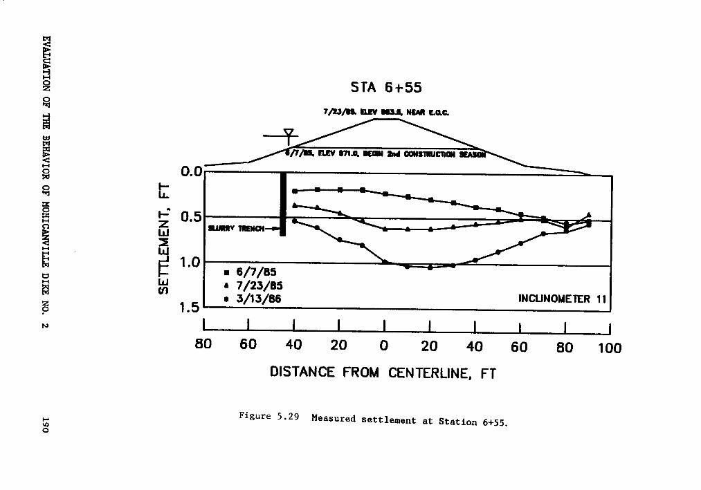
O__
O'.
I*
Zl*\
E0
V}
Q/.|
[UE
OW‘
ä.
O
Z;
Z;
¢LJ
ä5
—E
36
[—*
=·=ul
Gcz
umn
3E
[N
E“
5: *I
6co
gE
OU
E<
E5
Z§
ܤr'·¤
ä6
66
ä··
EE5
ä1
äZ
O[Z
.„6
äEm
8Q
ä:2
gh
äS2
Qä>
hk}
·¤PZ
•••O
0an
°°0
0.4
.4J.;|
°.LN3W3'LL.L3S
EVALUATION OFTIEBEHAVIOR OFMOHICANVILLE DIKE NO.2190
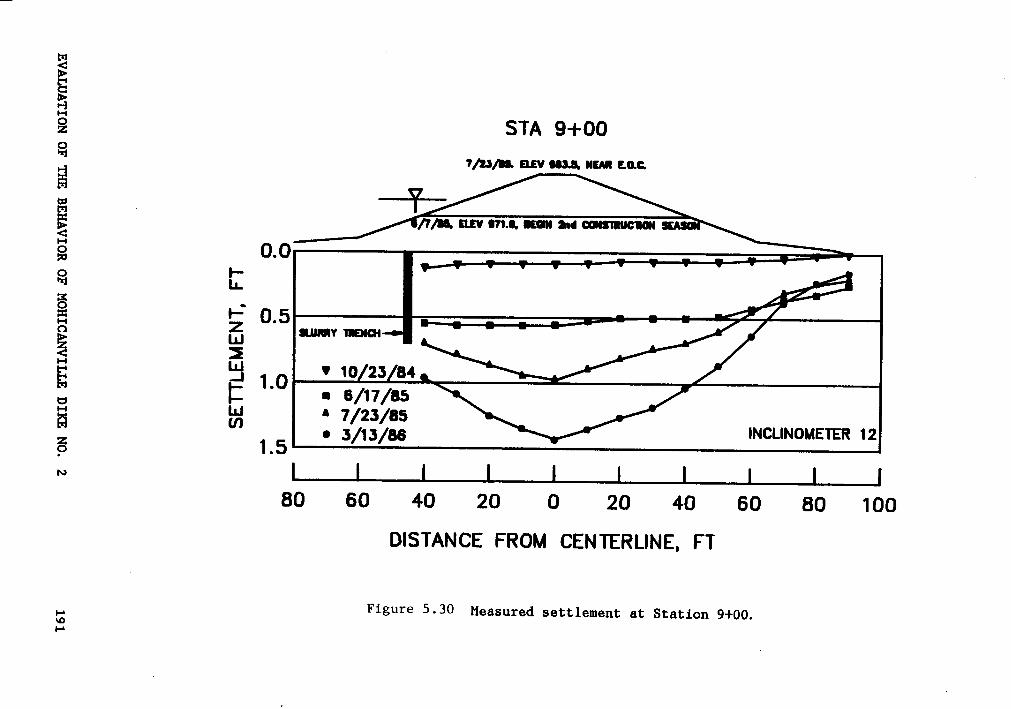
05:
E0[
‘\
ä°°
Nz
\‘6;
0.
‘N
°°3+
.1GSCi
_•
U
a3
“d
Z4-»
3'*
0¤=
'°N
M*5
QE
iI-
aaO
=Z
ä+
¢}
I6S
°’Ü
0E
§ä
EI
.2E
{E
0LL
ää
a°‘L6
*Ä
E3
<2
•-6
"«h
anil]
'°<<*3
@»6
Z5: g
EO
aiÜ
aäkä¤
äÜ
I (I
00
0.-S
.;
.L:.I°.I.N3W
3”I.L.|.3S
‘EVALUATION OFTIEBEIIAVIOR OFMOHICANVILLEDIKENO.2
191
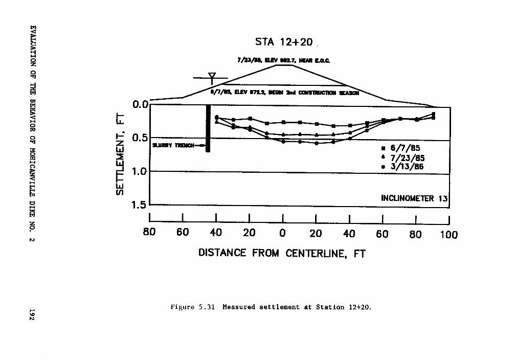
00YW
ID3
anm
q;O
{E}
°°Q
xäID
N!]
I1
I
Ou.
E:Ö
v-I
ä"°
LJ5
EE
ÜA
E.
3O
Mva
0E
NE
*.3N
äz
Uä
~s
'as9
AY
0ä
<E
QÜ
Ed
ggSS
QE
0“-
5Q
'°‘
u.:*5
'*ä
,ä
5G)
ä/
Q6
=•
WQ
06GJ
0E
‘°;E°
)•ä0
Q¤Q
0ID
°°0
0A
Aid
°.LN3W3'LL.I.3S
EVALUATIONorumßmmvxouorMOHICANVILLEum: No.2192
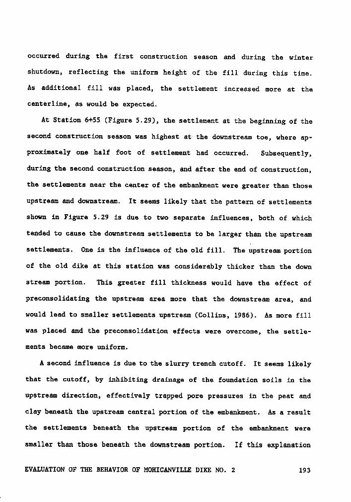
occurred during the first construction season and during the winter
shutdown, reflecting the uniform height of the fill during this time.
As additional fill was placed, the settlement increased more at the
centerline, as would be expected.
At Station 6+55 (Figure 5.29), the settlement at the beginning of the
second construction season was highest at the downstream toe, where ap-
proximately one half foot of settlement had occurred. Subsequently,
during the second construction season, and after the end of construction,
the settlements near the center of the embankment were greater than those
upstream and downstream. It seems likely that the pattern of settlements
shown in Figure 5.29 is due to two separate influences, both of which
tended to cause the downstream settlements to be larger than the upstream
settlements. One is the influence of the old fill. The upstream portion
of the old dike at this station was considerably thicker than the down
stream portion. This greater fill thickness would have the effect of
preconsolidating the upstream area more that the downstream area, and
would lead to smaller settlements upstream (Collins, 1986). As more fill
was placed and the preconsolidation effects were overcome, the settle-
ments became more uniform.
A second influence is due to the slurry trench cutoff. It seems likely
that the cutoff, by inhibiting drainage of the foundation soils in the
upstream direction, effectively trapped pore pressures in the peat and
clay beneath the upstream central portion of the embankment. As a result
the settlements beneath the upstream portion of the embankment were
smaller than those beneath the downstream portion. If this explanation
EVALUATION OF THE BEHAVIOR OF MOHICANVILLE DIKE NO. 2 193
N
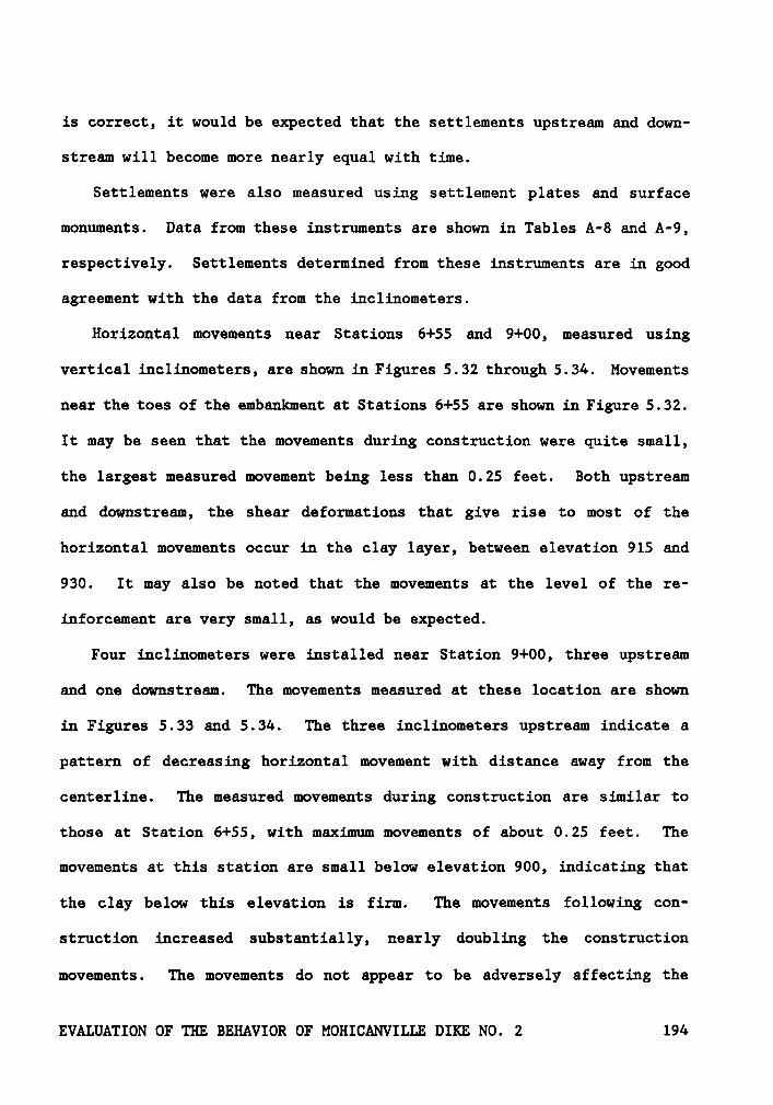
is correct, it would be expected that the settlements upstream and down-
stream will become more nearly equal with time.
Settlements were also measured using settlement plates and surface
monuments. Data from these instruments are shown in Tables A-8 and A-9,
respectively. Settlements determined from these instruments are in good
agreement with the data from the inclinometers.
Horizontal movements near Stations 6+55 and 9+00, measured using
vertical inclinometers, are shown in Figures 5.32 through 5.34. Movements
near the toes of the embankment at Stations 6+55 are shown in Figure 5.32.
It may be seen that the movements during construction were quite small,
the largest measured movement being less than 0.25 feet. Both upstream
and downstream, the shear deformations that give rise to most of the
horizontal movements occur in the clay layer, between elevation 915 and
930. It may also be noted that the movements at the level of the re-
inforcement are very small, as would be expected.
Four inclinometers were installed near Station 9+00, three upstream
and one downstream. The movements measured at these location are shown
in Figures 5.33 and 5.34. The three inclinometers upstream indicate a
pattern of decreasing horizontal movement with distance away from the
centerline. The measured movements during construction are similar to
q those at Station 6+55, with maximum movements of about 0.25 feet. The
movements at this station are small below elevation 900, indicating that
the clay below this elevation is firm. The movements following con-
struction increased substantially, nearly doubling the construction
movements. The movements do not appear to be adversely affecting the
EVALUATION OF THE BEHAVIOR OF MOHICANVILLE DIKE NO. 2 194
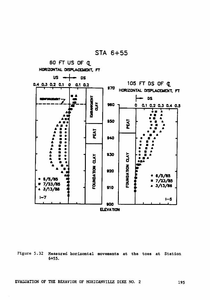
STA 6+5560 FT US OF Q_
Homzonw. nnsrucaearr, rrUS •-1-· ns
0.4 0.0 0.2 0.1 0 0.1 0.2 wo 105 FT 0S OF (EHORIZONTAL 01sP1.Ac£u¤n, rr
unuunm-7ä
1** DS''‘‘* * { ä 960 0 0.1 0.2 0..1 0.4 0.s
·
II I
· ä :: :":• 950 "• | A‘ . • I I I
A I •'l *A I • • '.l·*
: B40 • | A• • • 2 2 2{ { { • •:• I
: : : >- B30 >' • | A4 • •E Q • • •
A | • "‘A | • ¢I I ä
° F 920 E /=/as<•
52:%. § ä ·”==/·=. W/.5 ·~ ¤1¤ '·
‘°"°"‘
1'7 1-s000
ELEVATIDN
Figure 5.32 Measured horizontal movements at the toes at Station6+55.
EvALuA'r10N or um ßE11Av10R or MoH1cANv1LLE 0110:: No. 2 195
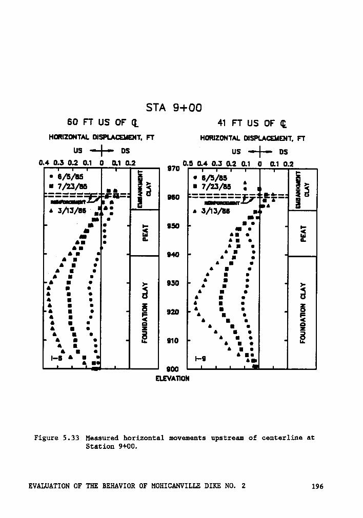
STA 9+00BOFTUSOFQ 41FTUSOF¢_
HGIIZCNTAL DISPLACEIADIT. FT HORIZONTAL DISPLAEAEIIT, FTus •-|-• os us •-I-• ns
0.4 0.5 0.2 0.1 0 0.1 0.2 97o 0.5 0.4 0.3 0.2 0.1 0 0.1 0.2•
7/2:/asä
• 7/23/B5 , >·::::: 5ggg4
J/13/aß I 4 3/13/I5 n..-
gl.!
=— II I ug‘· I . I In•· .‘.."1. .4: • 040 I I I
A | • ‘ F F. 6 I • F F F
· ·• .‘
1 1‘4: : >- 930 ‘ I I 9
I I I 4 n • jg g • { 1 { °I
‘ F F < 4 .| z EA | •g I D4 | • 2 F
' z• • • .. mo , 1, { ...4 • ••
· ·‘
.'..1- 4 1I 0 2 . I-0 ••
000 g‘
ELEVATION
Figure 5.33 Maasured horizontal movements upstream of centerline atStation 9+00.
EVALUATION OF THE BEI-IAVIOR OF MOHICANVILLE DIKE NO. 2 196
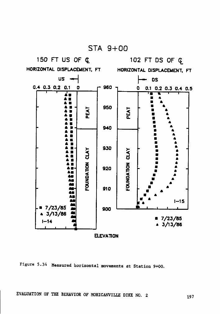
STA 9+00150 FT us OF Q 102 FT DS OF Q
Homzouun 01s1=•.Ac1-zusuv, rr 1-soanzoum. ouspucsusur, rrus •-·| |—·· 0s
0.4 0.: 0.2 0.1 0 960 0 0.1 0.2 0.: 0.4 0.622 : •• • 2
‘.2 2 *2 °5° *2 -
•j
=E E 2 2• •
'‘• ¤ 940 {‘,
‘' n •
I II
‘‘ ‘n •
I I.
•
11 ä ä : gA | Z Z .4 ° 920 ° '
‘•= 2 2 .· :2', 9 9 •·
_
I I
"u •
u I-15I¤ 7/25/85 . 90023/13/86'*"2 :/1:/66
Etzvnuou
Figvfé 5-34 Maasured horizontal movements at Station 9+00.
01- um nmvxox or u01ucANv11.1.¤ um No. z 197
embankment, as the reinforcement forces at this station are decreasing.
At elevation 960, the reinforcement elevation, the measured movements are
consistently downstream. As noted by Collins (1986), the movements appear
to indicate a downstream movement of the entire embankment.
An inclinometer located 128 ft upstream of Station 12+20 recorded
movements of less than 0.01 ft at all elevations during and following
construction.
5.7 Finite Element Analyses
As mentioned previously, finite element analyses were performed for
design by the Waterways Experiment Station (Fowler et al. 1983), and ad-
ditional analyses were performed after construction during this investi-
gation, in connection with evaluation of the results of the
instrumentation program. In both analyses the same computer program was
used, although modifications to the program were made as described in
Chapter III.
The degree of agreement between the actual stress-strain character-
istics of the soil and those modeled by CON2D can be checked by using the
parameters to calculate triaxial stress-strain curves, and comparing the
computed stress-strain behavior with experimental results. The determi-
nation of the model parameters for the foundation clay, peat and
embankment fill is discussed below. In selecting the parameters used in
the analyses, emphasis was placed on matching the actual behavior of the
soils in the small strain range, because it was known that the actual
_ EVALUATION OF THE BEHAVIOR OF MOHICANVILLE DIKE NO. 2 198
strains would be small if they matched the measured behavior of the
embankment.
Finite element analyses were performed on two of the instrumented
sections. Station 6+55 was analyzed because: (1) the foundation condi-
tions at this section were well defined and not affected by the previous
failure, (2) a significant depth of soft foundation clay existed (ap-
proximately 40 feet), and (3) the reinforcing was instrumented every five
feet upstream and downstream from the centerline, providing a unique op-
portunity to compare calculated and measured reinforcement forces. Ana-
lyses were also performed for Station 9+00 conditions to investigate the
effect of the double layer of reinforcement.
The effect of ageing of the embankment clay on the reinforcement be-
havior was studied through a laboratory testing program to determine the
effects of ageing on strength and stiffness, and through analyses per-
formed using properties for freshly compacted and aged samples of the
fill.
5.7.1 Selection of Soil Parameters
5.7.1.1 Foundation Clay
The available soil data on the foundation clay included three con-
solidated undrained (CU) envelopes from triaxial compression tests with
pore pressure measurement, several unconsolidated-undrained (UU) tests,
’and one dimensional consolidation tests, as well as classification data.
EVALUATION OF THE BEHAVIOR OF MOHICANVILLE DIKE NO. 2 199
A review of the test borings led to the conclusion that the foundation
clay was primarily a silty clay ranging from medium to high plasticity,
with occasional lenses of organic clay. Thus, the initial soil parameters
were developed from tests on clays with medium to high plasticity.
The determination of the soil parameters for the model used requires
consolidated drained or consolidated undrained triaxial compression tests
with pore pressure measurements and consolidation test data. For the
foundation clay two CU tests and four consolidation tests were available
which were performed on medium to high plasticity silty clay. These data
are shown in Figures 5.4 and 5.6, respectively. The parameters were de-
termined using the procedures developed by Duncan et al. (1981) and
D°Orazio and Duncan (1982).
The initial parameters determined were based on CU triaxial tests on
sample UD22-7 and the consolidation test from sample S16-3. The parame-
ters determined from these tests are shown in Table 5.3. The degree of
agreement between the actual stress-strain characteristics of the soil
and those calculated using the derived parameters can be checked by using
the parameters to calculate triaxial stress-strain curves, and comparing
the computed stress-strain behavior with experimental results. The com-
parison for the soft clay foundation material shown in Figure 5.35 for
confining pressures of 0.58 and 0.75 tsf, where it can be seen that the
computed stress-strain behavior underpredicts the strength of the soil
and overpredicted the pore pressures by a large margin. The next step
was to make adjustments to the parameters to obtain better agreement.
EVALUATION OF THE BEHAVIOR OF MOHICANVILLE DIKE NO. 2 200
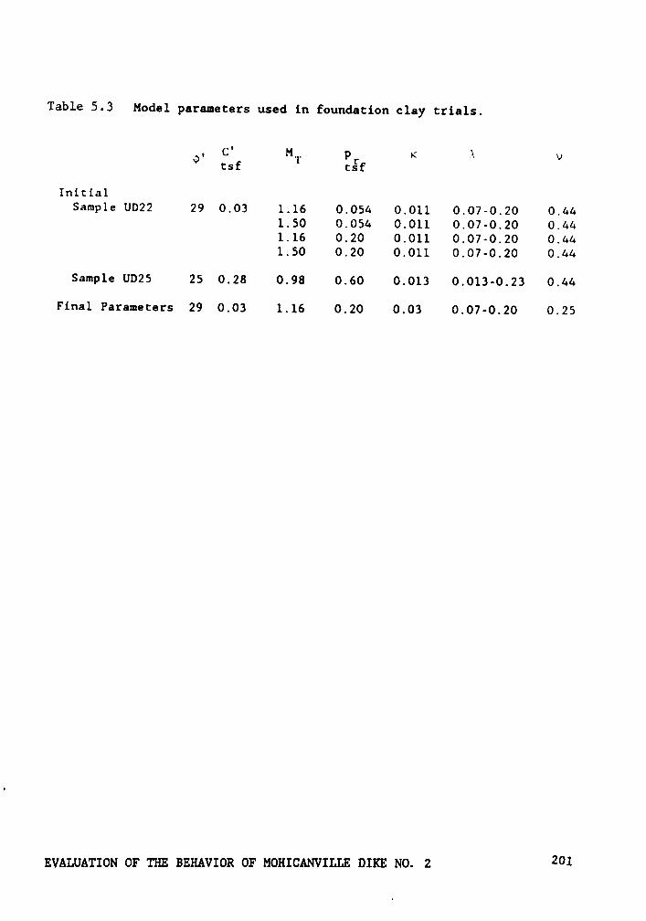
Table 5.3 Model paramecers used in foundation clay trials.
, C' M,, p rc Ä vQ csf l cgf
InitialSample UD22 29 0.03 1.16 0.054 0.011 0.07-0.20 0.44
1.50 0.054 0.011 0.07-0.20 0.441.16 0.20 0.011 0.07-0.20 0.441.50 0.20 0.011 0.07-0.20 0.44
Sample UD25 25 0.28 0.98 0.60 0.013 0.013-0.23 0.44
Final Parameters 29 0.03 1.16 0.20 0.03 0.07-0.20 0.25
EVALUATION OF THE BEHAVIOR OF MOHICANVILLE DIKE NO. 2 201
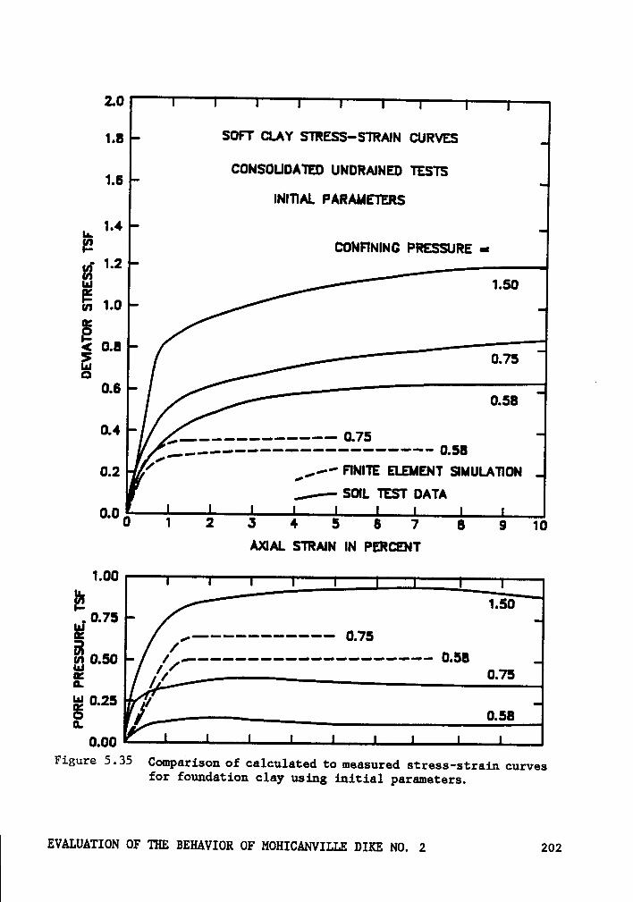
2.0
1.8 SOFT CLAY STRESS—STRAIN CURVES
15 CONSOUDATED UNDRAINED TESTSINITIAL PARAMETERS
Ä104
E CONFINING PRESSURE •8,; 1.2U
1.0
0.8Q .aj
0.58
°·* ___....------ 0.76______....----—-—-—·—--······ 0.58
g_2 FINITE ELEMENT SIMULATIONI. _;--SOIL TEST DATA
0°00 1 2 5 4 5 5 7 8 9 10AXIAL STRAIN IN PERCENT
ät 1.500.75S /,-------——-- 0.76
/1/.-----·-——-------——-·· UÖB 075E 1’
°
°“0.00Figure 5-35 Comparison of calculatad to measurad stress-strain curvas
for foundation clay us:Lng initial paramatars.
EVALUATION OF THE BEHAVIOR OF MOHICANVILLE DIKE NO. 2 202
To obtain larger computed strengths, the values of M and pr were in-
creased. The first change involved increasing M to 1.50 from 1.16 with
the results shown as curve B in Figure 5.36. Another trial, in which pr
was raised to 0.20 tsf from 0.054 tsf (keeping M = 1.16), was also per-
formed, with almost the same effect as increasing the value of M. It may
be seen that these changes raise the stress-strain curve closer to the
actual data, but also increase the magnitudes of the calculated pore
pressure. The effect of increasing both M and pr to 1.50 and 0.20 tsf
respectively is shown by curve C in Figure 5.36. The effect is to obtain
a relatively close fit to the ultimate strength, but the calculated
stress-strain curve deviates significantly from the measured curve and
the pore pressure response is still overpredicted.
The severe overprediction of pore pressures was of considerable con-
cern, and to obtain a better fit to measured pore pressures, the parame-
ters were further adjusted. D°0razio and Duncan (1981) studied the
effect of changes in parameter values on shapes of undrained stress-strain
curves and pore pressure curves with the qualitative results shown in
Figure 5.37. Parts b and c of this figure show that increasing x and v
should lower the calculated pore pressure response, but this also has the
effect of greatly altering the calculated stress-strain curve. Indeed,
when a change in only one of these parameters was made, large changes
would occur in the shape of the stress-strain curve.
At this point, data and from additional consolidation and triaxial
tests were further examined, revealing two important facts: First, the
initial value of x may have been somewhat low. Second, the test data used
EVALUATION OF THE BEHAVIOR OF MOHICANVILLE DIKE NO. 2 203
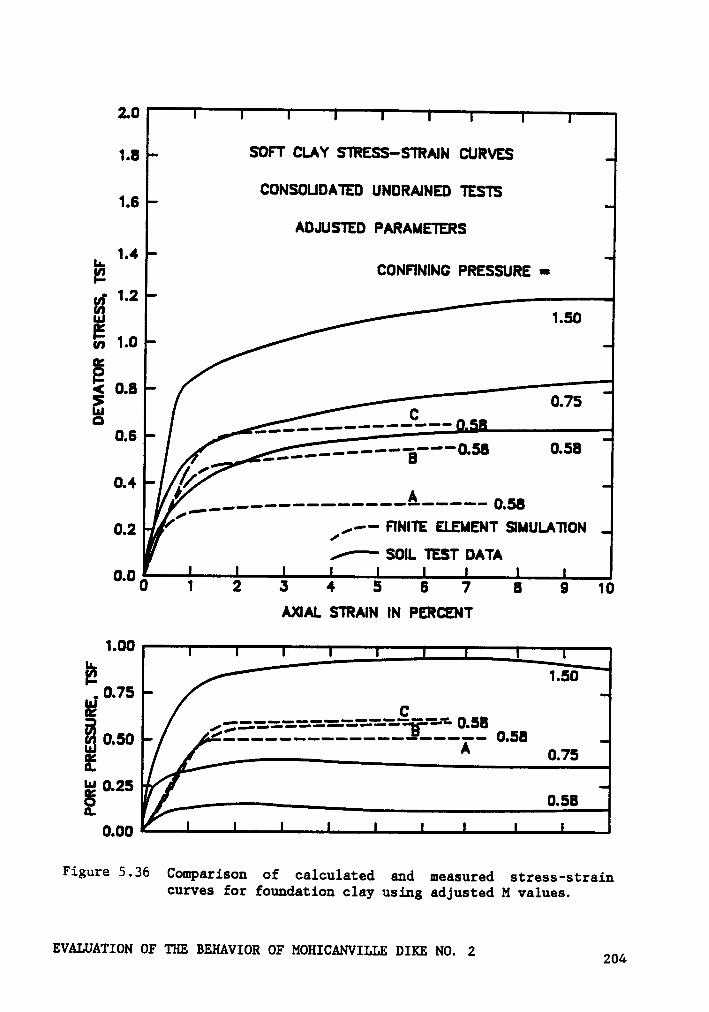
2.0Lg SOFT CLAY STRESS—STRAIN CURVES
16 CONSOUDATED UNDRAINED TESTSADJUSTED PARAMETERS1.4"“ CONFINING PRESSURE •I2
5- 1.21.00.8
Q • .Dj ___,...--·--***0.58 0.58•*"-B0.4 ________-...-------A——--- 0.58
0_20[
/,-- FINITE ELEMENT SIMULATIONZ'* SOIL TEST DATA0°¤0 1 2 5 4 5 6 7 8 9 10AXIAL STRAIN IN PERCENT1-*70 1äQ 1.500.75 C0,50 ’--——-—-—-—··——***'Ä"' °·”
0.75E ,
ä0.25Figure5.36 Comparison of calculated and measured stress—strain
curves for foundation clay using adjusted M values.
EVALUATION OF THE BEHAVIOR OF MOHICANVILLE DIKE NO. 2 204

Increasinq K
bm Incraasinq Ä 6**6-
·é
Increasinq K
EO gu
Increosing Ä
ä äIncreasinq K
gdEa
(a) (b)
— (I+e)p’*°'”TI uUI —•2
I2B60 _éq
Increcsinq Ké_ !¤¤•'¤¤$¤¤9 U 5. and Decreosinq U
Ed Ea
(I+e)p'B 'V T-U: L .. Eu.,
Incre¤singK 2 *28Increasinq and Decfeasißq U
$0 Cc(c) (d)
Figure 5.37 Effect of changes in soil parameters on shape of stress-strain curves (after D'Orazio and Duncan 1983).
EVALUATION OF TIE BEHAVIOR OF MOHICANVILLE DIKE NO. 2 205
for comparison purposes were from soil samples which were probably
slightly overconsolidated. The effect of adjusting x can be seen in
Figure 5.37b; as adjustments to x are made, either a "stiffer" or "softer"
stress-strain response can be be obtained. Interpretations of additional
consolidation test data showed x to be in the range of 0.018 to 0.024,
about twice as large as initially used. Also at this point, preliminary
analyses of the dike were being performed and one of the things considered
was the effect of Poisson°s ratio on the reinforcement forces computed.
It was found that using Poisson's ratio values as calculated from the test
data resulted in computed reinforcement forces much greater than those
measured in the field. A series of trials showed that Poisson's ratio
values of 0.25 for the peat and foundation clay provided the best match·
to field reinforcement forces. As the value of Poisson°s ratio was re-
duced from (0.44 to 0.25) it was necessary to raise x to maintain the
shape and slope of the stress-strain curve, similar to the effect shown
in Figure 5.37d.
The two samples used for the initial comparison, Figure 5.35, were
probably slightly overconsolidated. The stress paths for samples con-
solidated to these two confining pressures (0.58 and 0.75 tsf), shown in
Figure 5.38, show shapes normally associated with overconsolidated soils.
In contrast, the stress path for the sample having a confining pressure
of 1.50 tsf exhibits behavior more typical of normally consolidated clays.
Using the initial parameters with the higher confining pressure produces
the results shown in Figure 5.39. A very good match is obtained for the
stress-strain data from the test on the sample consolidated to 1.50 tsf.
EVALUATION OF THE BEHAVIOR OF MOHICANVILLE DIKE NO. 2 206
As was the case previously, the pore pressure response is overpredicted
by a large margin, although the match to the measured pore pressure is
better at low strains.
To ascertain whether the lack of agreement between computed and actual
stress-strain data was a consequence of the slightly overconsolidated
nature of the soil, additional parameter determination was performed
using the CU triaxial data from sample UD25-7. This sample was chosen
because, as shown in Figure 5.40, the stress paths for each sample com-
prising the envelope show characteristic normally consolidated behavior.
The derived parameters are shown in Table 5.3. Comparisons of the com-
puted and actual test data for this case are shown in Figure 5.41. Con-
solidation characteristics from sample UD25-6 were used in these
calculations. The stress-strain behavior is not simulated particularly
well and the computed pore pressures response is overpredicted. This
indicates that the overconsolidation of the soil samples in the first
trial may not be the sole reason for the lack of agreement between the
computed and actual curves.
Using a value of Poisson's ratio equal to 0.25, additional simulations
were performed with the aim of reducing the calculated pore pressure re-
sponse, while matching the initial parts of the actual stress-strain
curves. No variations of the parameters were found in which the pore
pressure response was changed more than 15 percent from that calculated
in the initial trial.
Consideration of the stress paths followed by the samples provide an
explanation. The yield surface used in the model is elliptical, as shown
EVALUATION OF THE BEHAVIOR OF MOHICANVILLE DIKE NO. 2 207
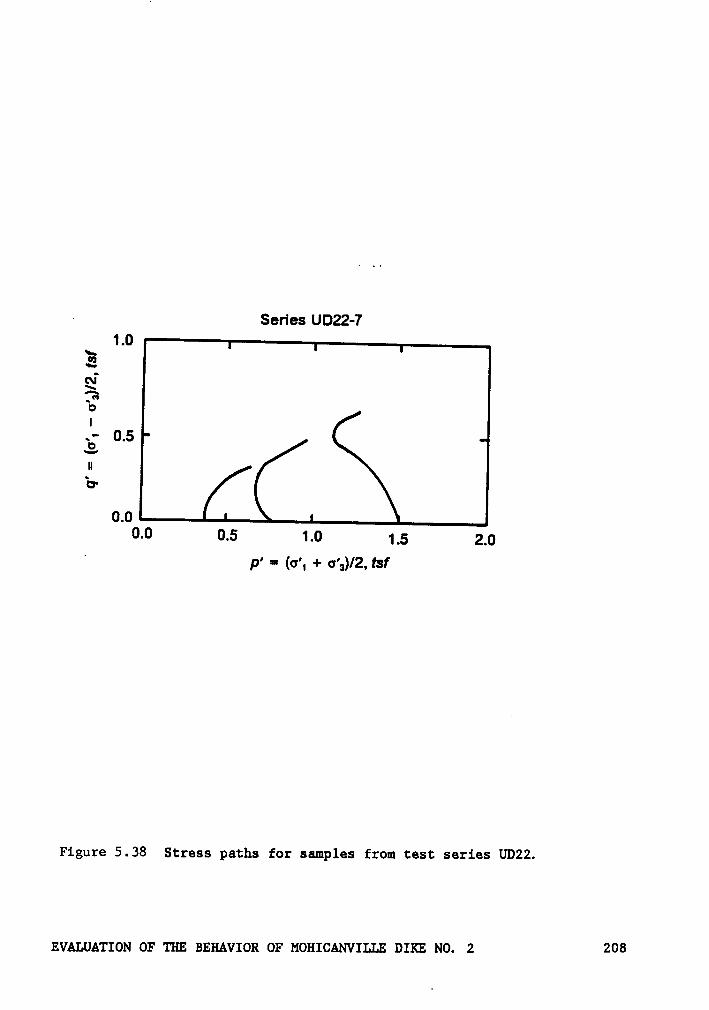
· Series UD22-71.0
°•~Z2Q?‘S’
u.- 0.53uB-
0.00.0 0.5 1.0 1_5 z_g
”p'
-(o', + cs',)/2, fsf
Figure 5.38 Stress paths for samples from test series UD22.
EVALUATION OF THE BEHAVIOR OF MOHICANVILLE DIKE NO. 2 208
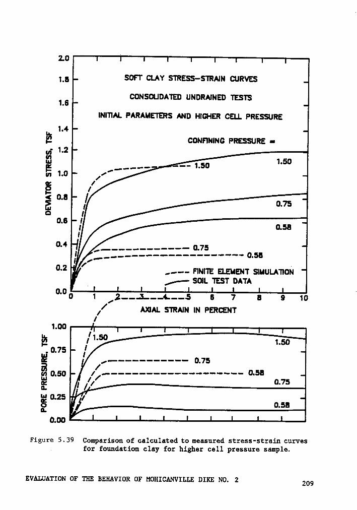
2.01
1.8 SOI·"I' CLAY STRESS-STRAIN CURVES
16 CONSOLIDATED UNDRAINED TESTSINI11AL PARAMETERS AND HIGHER CELL PRESSURE[__ 1.4
E CDNFINING PRESSURE •
V; 1.23
1.0//’-_
1§ 1< 0.8 [Q 1
0 6Il° [ 0.58
I9-* __.....-..--- 0.75
I ___,-....----——---—--—--— 0.58I /¤"" _°·2 [Ip ,....- nmz asusuv smuu.A110u_ Z- 50IL TEST DATA
°°00 1 /2....-.J.....A...-5 6 7 8 9 10// AXIAL STRAIN IN PERCENTI1.00 1;;:ä 1.50
uf 0.750: /,————---———— 0.75ä 0.50 /1/·-—--—----—-———————- 0-58
0 75E I 1’ °
W 0.25I: II0000
Figure 5.39 Comparison of calculated to measured stress-strain curves. for foundation clay for higher cell pressure sample.
EVALUATION or um ummvxoa or 1~10H1cANv1LL1·: 01KE No. 2 209
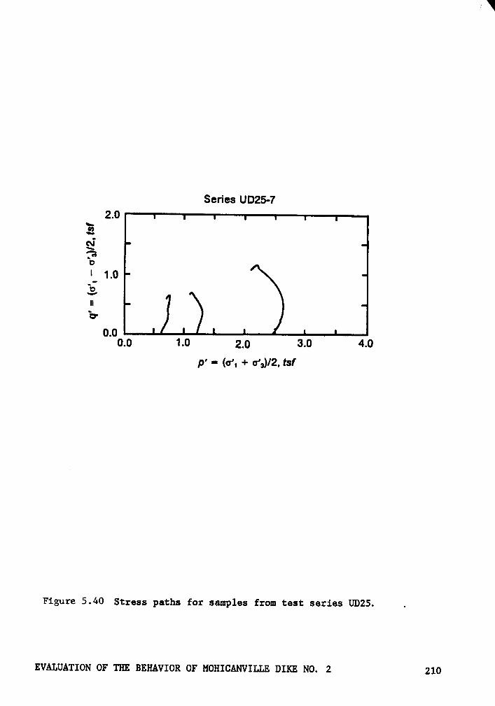
» Y
Series UD25·72.0
\•
.*2Q‘é’‘_
1.032
uB
0.00.0 1.0 2.0 3.0 4.0
p'-
(cs', + o',)/2, fsf
Figure 5.40 Stress paths for samples from test series UD25. .
EVALUATION OF THE BEHAVIOR OF MOHICANVILLE DIKE NO. 2 210
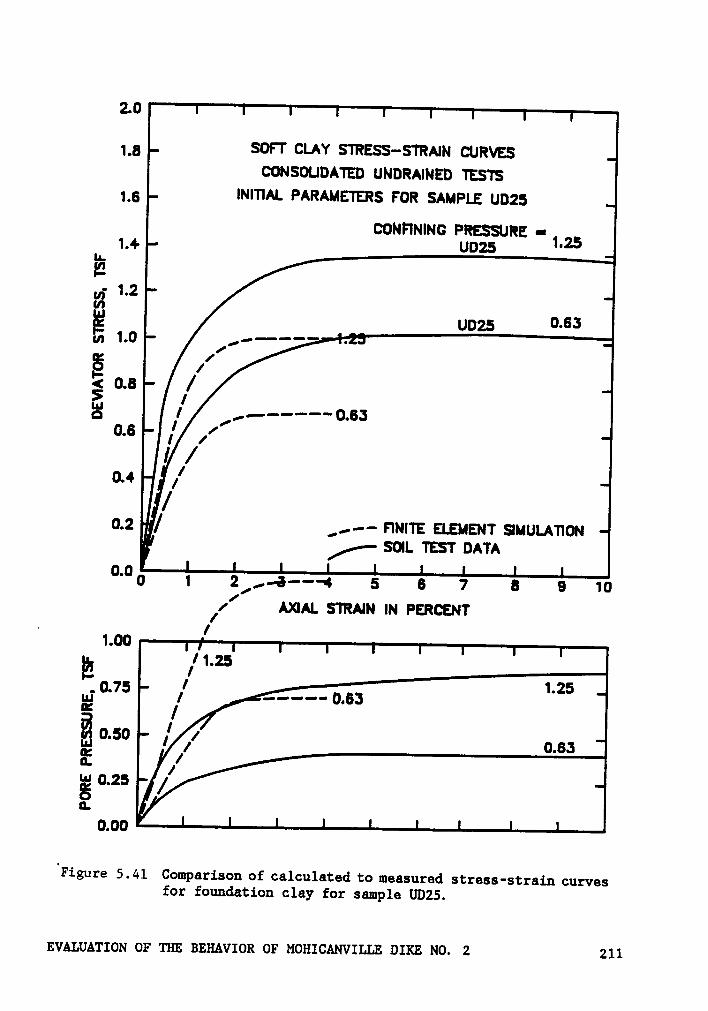
2.0
1.8 SOFT CLAY STRESS—-STRAIN CURVESCONSOLIDATED UNDRAINED TESTS
1.6 INITTAL PARAMETERS FOR SAMPLE UD25
CONFINING PRESSURE • 1|25LLEU; 1.2tnE Ugzg 0.63m 1.0 ,••i""° •
6/'2 0.s /E 1Q I ,•—•**"'*'O.63
05 II rf,
I /0.4
'
/0.2 _„·-—
FINITE ELEMENT SIMULATIONL (— SOIL TEST DATA°‘°0 1 2/,-6---4 s 6 7 a s 10/// AXIAL STRAIN IN PERCENT· I1.00
0.75 *25—--··· 0.63
{ 1W 0 25 /g /0.
0.00
'Figure 5.41 Comparison of calculated to measured stress-strain curvesfor fouudation clay for sample UDZS.
EVALUATION OF THE BEHAVIOR OF MOHICANVILLE DIKE NO. 2 211
in Figure 5.42. A soil sample subjected to a confining pressure has an‘initial mean stress, p’=
oa As deviator stress is applied to the sample,
the total stress path (TSP) follows curve A for triaxial conditions and
curve B for plane strain conditions. The effective stress path (ESP) will
follow the elliptical yield surface, the exact path to the failure surface
being dependent upon the model parameters used in the calculations. The
pore pressure generated will be the difference between the ESP and the
TSP as shown in Figure 5.42. It is believed that the shape of the yield
surface (cap) in the model leads to the large induced pore pressures and
a different definition of the cap would be required to reduce the pore
pressure response.
After concluding that it was not appropriate to attempt to match the
triaxial pore pressures in plane strain calculations, the final parame-
ters for the soft foundation clay were chosen based on these consider-
ations: (1) a value of Poisson°s ratio of 0.25, (2) a value of x
consistent with Poisson's ratio to reasonably match the first part of the
stress-strain curves, and (3) values of M and pr determined from strength
values from sample UD22, since these values ( ¢’=29°,c'=0.03 tsf) are
reasonably close to the "design" values of ¢'= 28°, c°=0.09 tsf adopted
by Collins et al. (1982) for the stability analyses. The results obtained
are shown in Figure 5.43 and Table 5.3. Slightly steeper stress-strain
curves than those measured for specimens from UD22 were used in consid-
eration of the stiffer stress-strain response of samples from UD25.
EVALUATION OF THE BEHAVIOR OF MOHICANVILLE DIKE NO. 2 212
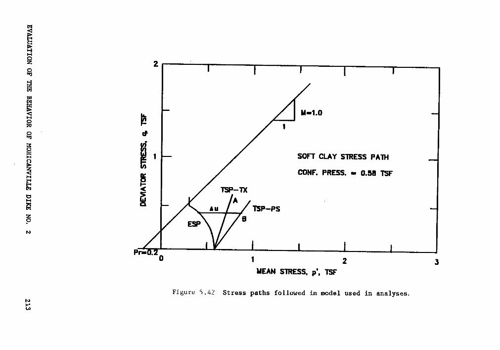
n
vi3u,
Ü
ä*3
3Q
3.6
VI
°-6;
iä'
3va
viN
Z>-
ܤ·
35
¤=E
OIL
·E
QO
__
•G
•61
Y2
26..
;S
ve0
vig
No
..E
:vv
.2E
ä2
E‘
33•··
C6.
Ü'°
3•
<3
Q3
Z:6u
hGJ-
$-63cmLE
c61
„-‘
_JS
].°b
°SS3EI.I.SUO
.l.VI/GG
[¤.
EVALUATIO
NO
FTHE
BEHAVIO
RO
FM
OH
ICAN
VILLED
IENO.
2213
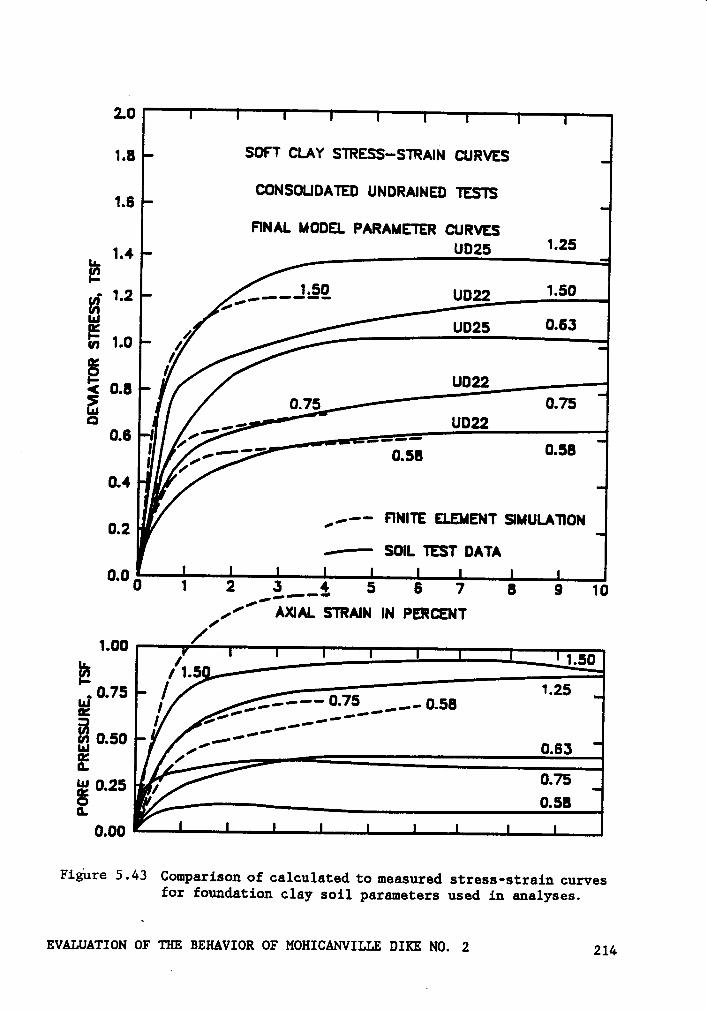
2.0
1.8 SOFT CLAY STRESS-STRAIN CURVES
15 CONSOLIDATED UNDRAINED TESTSFINAL MODE. PARAMETER CURVES
·I2. L2 _..-J.§Q U022
‘·5°I2 #’ul
1.0}/
/§ 1ä 0.8Q
. I ..-.-—_ 0 61 0 58 0.58
°
0.4
0 2’„-· FINITE ELEMENT SIMULATION
I e—·— SOIL TEST DATA°‘°0 1 2 g____2_ 6 6 7 6 9 10
AXIAL STRAIN IN PERCENT
I1 250.75 °1.: _---·-- O-75 _,..- 0.58°‘ ,·’ ..···"'”
0.63/Lu 0.75E 0.66‘*0.00
Figure 5.43 Comparison of calculated to measured stress-strain curvesfor foundation clay soil parameters used in analyses.
EVALUATION OF TIE BEHAVIOR OF MOHICANVILLE DIKE NO. 2 214

5.7.1.2 Peat
The selection of constitutive parameters for peats is difficult given
their complex nature and the current state of knowledge of their behavior.
The fibrous nature of peat materials gives them unique properties. The
consolidation behavior of peats is much different than that of clays, and
has been the subject of much recent research (Landva and La Rochelle,
1983; Dhowian and Edil, 1980; and Lefebrve et al. 1984). Secondary com-
pression plays a significant role in the consolidation behavior of peats
and thus classical one·dimensional consolidation theory is often not a
good predictor of their behavior.
Data from triaxial compression tests on peats frequently show high
friction angles, approaching 50° or more (Landva and La Rochelle, 1983;
Edil and Dhowian, 1981; and Rowe et al. 1984). For an analysis of a
geotextile reinforced embankment, Rowe et al. (1983) conducted triaxial
compression, uniaxial tension, direct shear, and simple shear tests on a
peat. The triaxial tests yielded values ofV’=S4°
and c'=0, while the
direct shear and simple shear tests gave values of¢’=27°,
c'=3 kPa and
V =26°, c'=1.1 kPa, respectively. In the finite element analyses per-
formed using these test results, Rowe et al. found the agreement with
measured embankment performance to be much better using parameters from
simple shear and direct shear tests.
The permeability of peats, with their open structure, is dependent
on the amount of mineral matter present in the peat, the degree of con-
solidation and the extent of decomposition (MacFarland, 1969). The re-
EVALUATION OF THE BEHAVIOR OF MOHICANVILLE DIKE NO. 2 215
lationship of decreasing permeability with increasing consolidation
pressure (load) has been discussed by Weber (1969), Lefebrve et al. (1984)
and others. The relationship shown in Figure 5.9 has been adopted herein
and the permeability of the peat was considered to be a function of
overburden pressure corresponding to the line shown. Lefebrve et al.
(1984) and Dohowian and Edil (1980) report substantial anisotropic
permeability in peats, with the horizontal permeability often an order
of magnitude greater than the vertical permeability.
Consolidated undrained tests on the foundation peat show much scatter.
Interpretation of the data results in¢’
values between 17° and 34° and
c' values between 0 and 0.18 tsf. Two consolidated drained tests were
performed on the peat giving o' =11° and c'=0.14 tsf. In light of the
scatter in the results, values of M=1.0 and pr =0.15 tsf were selected,
corresponding to ¢'=25.4° and c'=0.07 tsf.
From the one-dimensional consolidation tests performed, values of A
ranging between 1.3 and 2.2 were determined. The smaller A values cor-
respond to the lower void ratios, eo about five, versus so values of seven
to nine for the higher values. A value of 1.3 was selected for the ana-
lyses. From the drained triaxial tests, values of Poisson°s ratio were
determined to be 0.115 and 0.23 at mean pressures of 0.40 tsf and 1.0 tsf
respectively. Values of Poisson°s ratio for peats in the range of 0.1
to 0.2 have been reported for peats (MacFar1and, 1969 and Rowe et al.
1984). Based on preliminary analyses, a value of 0.25 was used, as in
the WES analyses. Values of x determined from the test results ranged
from 0.13 to 0.26, with a value of 0.20 used in the analyses.
EVALUATION OF THE BEHAVIOR OF MOHICANVILLE DIKE NO. 2 216
Comparisons of the computed and measured stress-strain and pore
pressure behavior are shown in Figure 5.45. The agreement for the
stress-strain curves is fair, while the agreement for the pore pressure
curves is remarkably good.
5.7.1.3 Embankmeut Fill
Test data available for the embankment fill included four CU tests
and an isotropic compression test. The CU data is summarized in Table
5.4, along with values of M and pr calculated for each test. The four
tests give very consistent values of ¢' and c'. Interpretation of the
isotropic compression test data shown in Figure 5.12 produced values of
A =0.052 and x =0.0075. The data from CU test 85R-2 was used to evaluate
Poisson's ratio, the resulting value being 0.30.-
Using a value of M=1.29 and pp=0.3O along with other parameters as
described above, the computed stress-strain curve shown in Figure 5.45
was obtained, for a confining pressure of 0.50 tsf. The fit to the actual
stress-strain data is very good for strains below three percent. The
measured pore pressure response could not be simulated by the model; no
attempt was made to achieve better agreement for the pore pressure data.
In Figure 5.46 it may be seen (curve A) that the above parameters do not
provide a good representation of the stress-strain behavior of the new
fill. The curve shown as B in this figure was obtained by trial and has
strength values of M=1.80 and p;=0.30. A value of x equal to 0.005 used
to generate curve B, compared to a value of 0.0075 for curve A.
EVALUATION OF TH BEHAVIOR OF MOHICANVILLE DIKE NO. 2 217
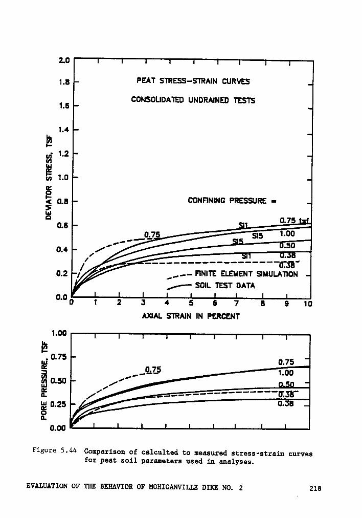
2.0
1.8 PEAT STRESS-STRAIN CURVES
16 CONSOLIDATED UNDRAINE0 TESTS
1.4u19 1.2
1.00:
aj CONFINING PRESSURE •SE 0.750.6 ·
@75gf
F1I0.4 _ _ L
/ ---—-—----——————···OTsa'g_g _„-- FINITE ELEMENT S1MULA'110N
g- S0|L TEST DATA
0°001234567B910AXIAL STRAIN IN PERCENT
1.00
. 0.75ää I I{ ____,....-———-····*""'''“”{ISB"
0.00
Figure 5-44 Comparison of calculted to measured stress-strain curvesfor peat soil parameters used in analyses.
EVALUATION or um BEHAVIOR or M0u1cANv1LL6 DIKE No. 2 218
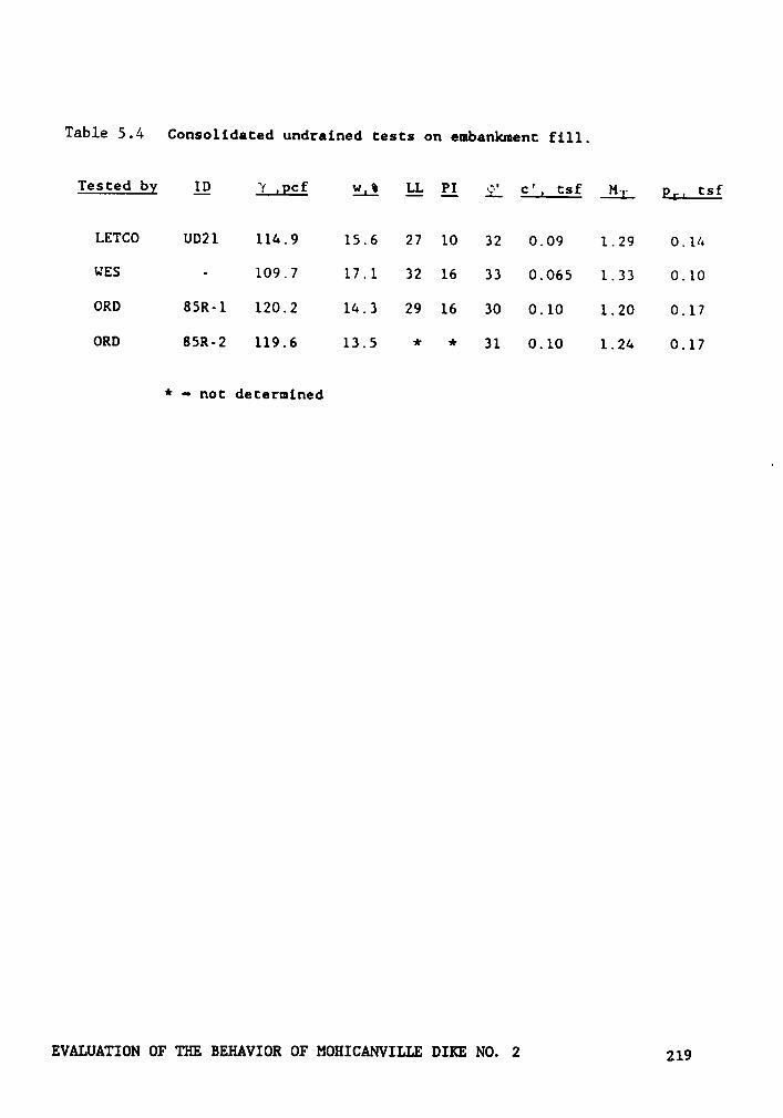
Table 5.4 Consolidated undrained tests on embankment fill.
Tested by LQ Y lgcf yyj Lg Q1 gl c', tsf MT gz. tsf
LETC0 UD21 114.9 15.6 27 10 32 0.09 1.29 0.14
UES - 109.7 17.1 32 16 33 0.065 1.33 0.10
ORD 85R-1 120.2 14.3 29 16 30 0.10 1.20 0.17
ORD 85R·2 119.6 13.5 * * 31 0.10 1.24 0.17
* - not determined
EVALUATION OF THE BEHAVIOR OF MOHICANVILLE DIKE NO. 2 219
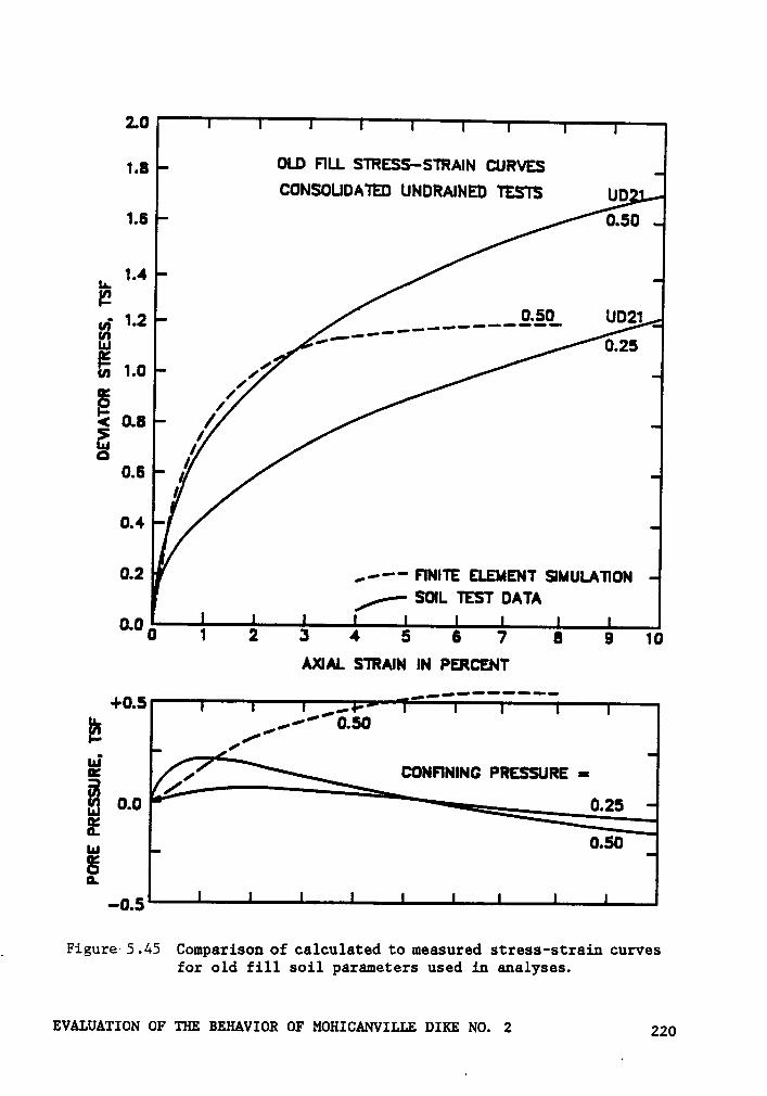
2.0
1.8 OLD FILL STRESS—STRAIN CURVESCONSOLIDATED UNDRAINED TESTS UD
1.6 0.50
un 1.4IB„; 1.2 ___..-£·§.‘L U¤21
E """” 0.25„1.0E
/< 0.a /5* I‘ä
II¤•6I
0.4
0.2'
5-** FINITE ELEMENT SIMULA'|'|ONZ- SOIL TEST DATA
°°00 1 2 3 4 5 6 7 8 9 10AXIAL STRAIN IN PERCENT
+0.6 _ -"""'°_--_—”
/"EH
counmuc Pnsssuns •
ä 0.0E
0.25¤.un5¤.
-0.5
_ Figure· 5 .45 Comparison of calculated to measured stress-strain curvesfor old fill soil parameters used in analyses.
EVALUATION OF THE BEHAVIOR OF MOHICANVILLE DIKE NO. 2 ggg

4.0
3_6 NEW FILL STRESS-STRAIN CURVESCONSDLIDATED UNDRAINED TESTS
3.2CONFINING PRESSURE •
u_ 2-8 0.75 tsE 66112V; 2.4$1
2.0 0 •
0.25§< 1.6 B
•5
11.2 '
___________&__
"„¢’°-_0.a
;/ I,-—FINITE ELEMENT SIMULA110N· /
V g-—SOIL TEST DATA
°'°o12:s-16676010AXIQL STRAIN IN PERCENT,/" ---—————
+0.5 _, ‘°
0.05
äé Vä 0.0 0.75Z 0.60S i0.
-0.6 *
Figure 5.46 Final stress-strain curves used for new embankment fill.
EVALUATION OF THE BEHAVIOR OF MOHICANVILLE DIKE NO. 2 221

5.7.1.4 Summary of Soil Model Parameters
The soil model parameters used in the analyses of the reinforced
embankment are summarized in Table 5.5.
5.7.2 Analysis of Station 6+55
Station 6+55 is well suited for analysis because the foundation con-
ditions are relatively well defined from the test boring program, and the
1930's failures did not impact this area. Additionally, because the soft
clay is relatively deep in this location, and some of the highest re-
inforcement forces were measured in this area, analysis efforts were
concentrated at this station. The foundation conditions shown in Figure
5.15 were reproduced in two half—section meshes representing conditions
downstream and upstream of the centerline, as shown in Figures 5.47 and
5.48.
The analyses represented, as closely as possible, the actual con-
struction sequence. Being a post-construction analysis, layer heights
and dates of fill application were well known. The analyses began from
an elevation of 962.5 feet to correspond to the elevation of fill when
the strain gages were placed on the reinforcement. Initial stresses in
the foundation were chosen to reflect overburden pressures at this time.
The overburden pressures due to the old fill prior to its removal to el-
evation 960 feet were used as the preconsolidation stresses. Embankment
construction was simulated in five construction layers and several con-
EVALUATION OF THE BEHAVIOR OF MOHICANVILLE DIKE NO. 2 222
T
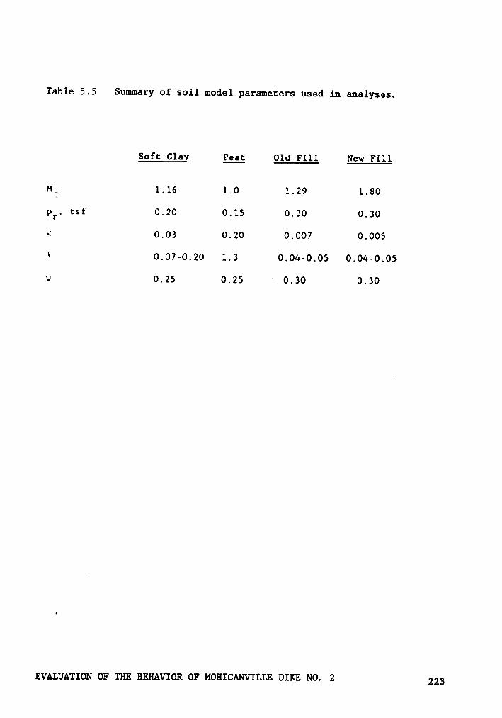
Table 5.5 Summary of soil model parameters used in analyses.
Soft Clay Peac Old Fill New Fill
M1. 1.16 1.0 1.29 1.80pr, tsf 0.20 0.15 0.30 0.30M 0.03 0.20 0.007 0.005
\ 0.07-0.20 1.3 0.04-0.05 0.04-0.05
v 0.25 0.25 0.30 0.30
EVALUATION OF THE BEHAVIOR OF MOHICANVILLE DIKE NO. 2 223
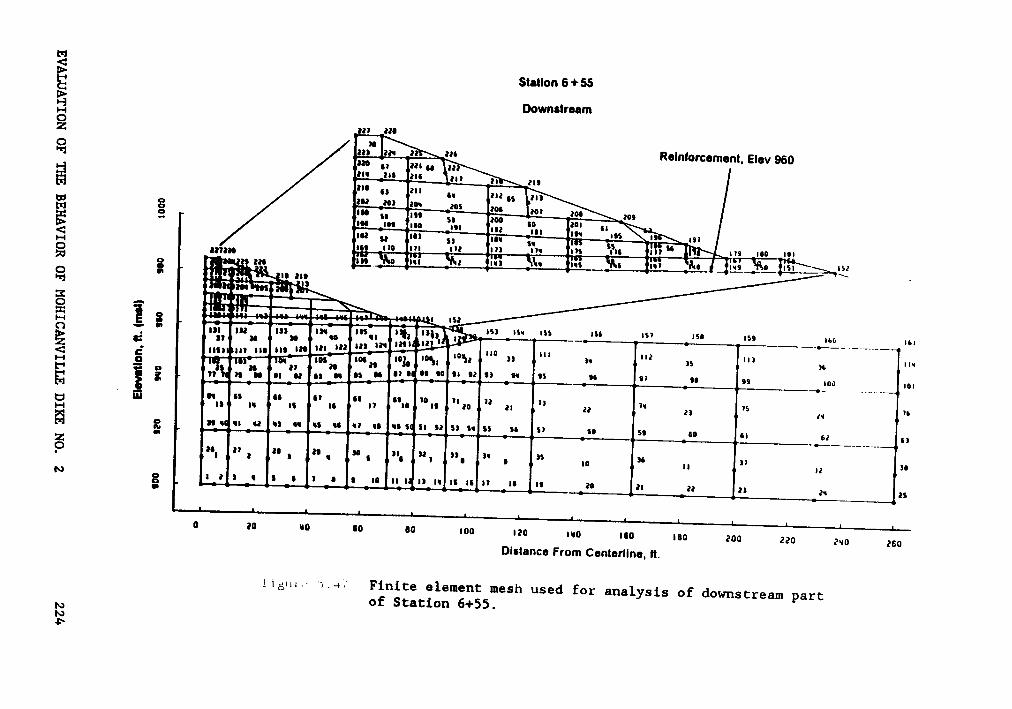
1!
„T8
21
1¥
2gl
’vu
ÄLJ
1T
j;g
22[
2E
2.
.13
ä2
TE
E=
2:
:.··
ä*2
E2"
§
§E-2
E..
1;5
2E
2.
-2ä
S —~
·
_:2
,2
..2
.2
*··§
Eg
1”
°°"
g(8
U3
*—-¤
22
22
„._
„_
*2;3
2g
2‘'"**·
2=
*7*2
E2:
2:E
22
E.,;
·¤
E2
.2E
RR
E22
E2
- 2B
älg22
·· 2g
’·
-2
****
·•-I(B
..
EE
RR
;"’=
4;
••-Ill-l—
2JE
EE
E"°
2. Gär2R
RQ
000l0•6
uu
uns026
ng;(nw) ‘u‘¤¤n••^•na
EvA1.uA·1·1oNOF
ummmvxoxz
OFMOHICANVILLE
DIKENo.
z224
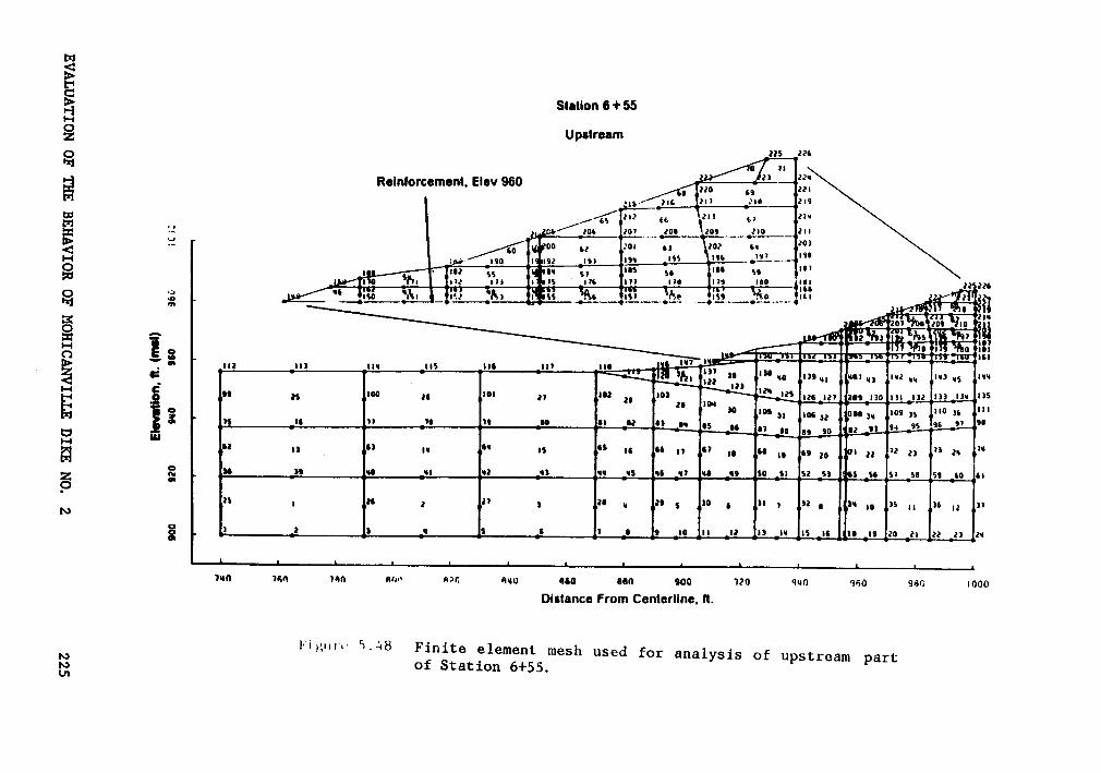
Eä
gé
éä
EE
E:
2;
;,;
§N
_—
E«•
••
·~
c'
,'·
s2
u•$
'l’-‘.
—9
llÜ
_:
:2
;Ü
ääää ~ ~—J-
.
IQIIEEEE
3I4_
II
Icr
g'
=.‘·I
I“
=-
eI,aI.;.;I’
**5·
zä S^‘I·,'•
I‘o
II
=”·
2‘.:~
,·I
·Q
;•
·E
22
==g
s..§
•·E-ZI_
"E°
^·$°'
‘'”
‘2
I4I
Ig
oU
,,Q
,,..^..,,;•
•~
•~
IU
Q-‘
In:2
22
22
:2
$E
,¤+
§·
°Q
ab0
2-
‘·In
g2
\°,
„,
"u
':3
2Q
Ya!2**
82
:‘
°°
"···
.„.
‘%$
·=·
EB
=·
ma
ma
..».‘2
°:>
ä+
83
*s‘°
g¢=
¢:¢2
„.§m
I’
°g5
.I
2c:
Q-
*•·¤I'~¢-4n
-Lu
O%
"’-
ÜÜ
egx
2IE
7
,E
gS;
E
:CZ
:6aeoss
ossam
ozs¤o•
(I•¤•VII'¤¤II•^•I3
EVALUATIONOF
THEBEHAVIOR
OFM
OHICANVILLEDIKE
NO.2
225
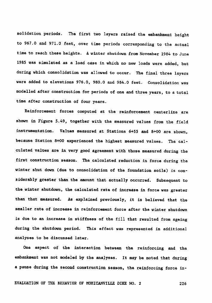
solidation periods. The first two layers raised the embankment height
to 967.0 and 971.0 feet, over time periods corresponding to the actual
time to reach these heights. A winter shutdown from November 1984 to June
1985 was simulated as a load case in which no new loads were added, but
during which consolidation was allowed to occur. The final three layers
were added to elevations 976.0, 980.0 and 984.0 feet. Consolidation was
modelled after construction for periods of one and three years, to a total
time after construction of four years.
Reinforcement forces computed at the reinforcement centerline are
shown in Figure 5.49, together with the measured values from the field
instrumentation. Values measured at Stations 6+55 and 8+00 are shown,
because Station 8+00 experienced the highest measured values. The cal-
culated values are in very good agreement with those measured during the
first construction season. The calculated reduction in force during the
winter shut down (due to consolidation of the foundation soils) is con-
siderably greater than the amount that actually occurred. Subsequent to
the winter shutdown, the calculated rate of increase in force was greater
than that measured. As explained previously, it is believed that the
smaller rate of increase in reinforcement force after the winter shutdown
is due to an increase in stiffness of the fill that resulted from ageing
during the shutdown period. This effect was represented in additional
analyses to be discussed later.
One aspect of the interaction between the reinforcing and the
embankment was not modeled by the analyses. It may be noted that during
a pause during the second construction season, the reinforcing force in-
EVALUATION OF THE BEHAVIOR OF MOHICANVILLE DIKE NO. 2 226
IIä 20ZOP
16g FEM ,g sm 6+55 Cni 12 STA 8+00
·
UJgl
8 /1 // /g 1,./
4"/I
VuJIZ
0 l
0 4 8 12 16 20 24FILL HEIGHT ABOVE ELEV 960, FT
Figure 5.49 Measured versus calculated reinforcement forces at thecenterline of Station 6+55.
EVALUATION OF 'I'IE BEHAVIOR OF MOHICANVILLE DIKE NO. 2 227
creased. As mentioned previously, it is believed that this increase in
force is due to undrained creep in the foundation peat and clay. A sim-
ilar increase near the end of construction is also believed to be due to
creep effects. Because the modified Cam Clay model used in the analyses
does not simulate creep effects, the finite element analyses do not sim-
ulate this aspect of the actual behavior. The field data indicate that
after a period of three or four weeks the effects of creep die out, and
the reinforcing force begins to decrease as the foundation soils consol-
idate.
Calculated distributions of reinforcing force across the embankment
are compared to the measured values in Figure 5.50. The calculated dis-
tributions are discontinuous at the centerline because they were calcu-
late using two half—meshes rather than a whole mesh. It can be seen that
the agreement is quite good overall, especially for the downstream half
of the embankment. The behavior of the upstream half of the embankment
was apparently affected to some degree by the slurry trench cutoff. Be-
cause the cutoff was represented in the analyses by only one element's
width, its interaction with the foundation and the embankment, and its
effect on the behavior, may not have been accurately reflected in the
calculated results.
Calculated pore pressures are compared to the measured values in
Figures 5.51 and 5.52. The calculated values are smaller than the meas-
ured values at the early stages, and larger than the measured values at
the later stages. These differences appear to be consistent with the
differences between the calculated and measured laboratory pore pressures
EVALUATION OF THE BEHAVIOR OF MOHICANVILLE DIKE NO. 2 228
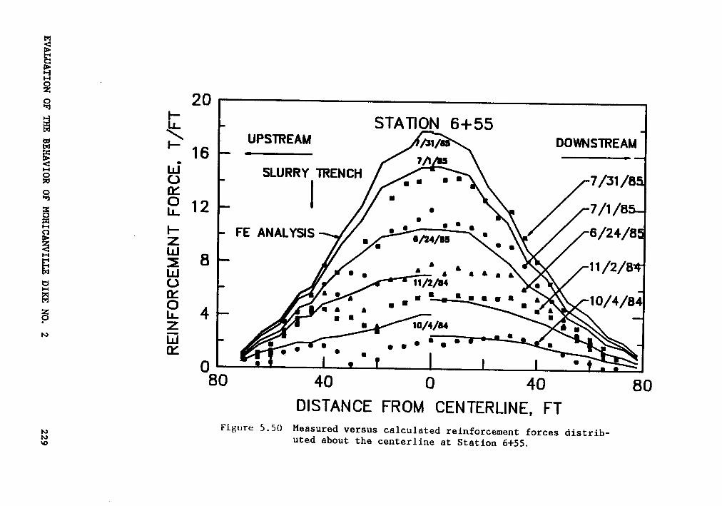
cE
Q„
QU
J•"
*N
ä'
EQ
\Q
8vw
r~r~
coZ„-V
Jä
/.
{°
8Q
/[-·
va/
II
|_I_¤>
.¢¢¤
8·
gEa
••
•_
_g
c;‘
*‘|
g¤
{Q·
-E
ääÄ
QH
4-J
Z.°
Q‘
='
E•
g<
°°
ccEB
I1I
IU
-U
ä(fl
•°
I.
. ..
Lö
wQ
I1
II
Z>
Uä
•an
•·g'§
•I
•H
<¤
EE
_—
°E
Q-
älä<
ggQ
•Q
Ä‘5°
LuM
„.I•·
E3
<E
Qnn
Q“·Q
cx.00
gco
N¤¤
Q-O
F*
1*
J.:]/J.°3OHO:I
LNBWHOEIOJNIHH
.w:vAr.u.mouorum
mmvxouoruouxcmvxm
mm:No.z
zzs
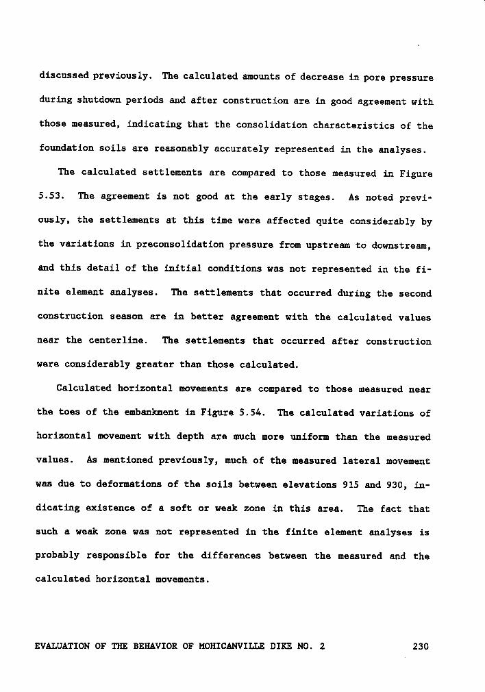
discussed previously. The calculated amounts of decrease in pore pressure
during shutdown periods and after construction are in good agreement with
those measured, indicating that the consolidation characteristics of the
foundation soils are reasonably accurately represented in the analyses.
The calculated settlements are compared to those measured in Figure
5.53. The agreement is not good at the early stages. As noted previ-
ously, the settlements at this time were affected quite considerably by
the Variations in preconsolidation pressure from upstream to downstream,
and this detail of the initial conditions was not represented in the fi-
nite element analyses. The settlements that occurred during the second
construction season are in better agreement with the calculated Values
near the centerline. The settlements that occurred after construction
were considerably greater than those calculated.
Calculated horizontal movements are compared to those measured near
the toes of the embankment in Figure 5.54. The calculated Variations of
horizontal movement with depth are much more uniform than the measured
values. As mentioned previously, much of the measured lateral movement
was due to deformations of the soils between elevations 915 and 930, in-
dicating existence of a soft or weak zone in this area. The fact that
such a weak zone was not represented in the finite element analyses is
probably responsible for the differences between the measured and the
calculated horizontal movements.
EVALUATION OF THE BEHAVIOR OF MOHICANVILLE DIKE NO. 2 230
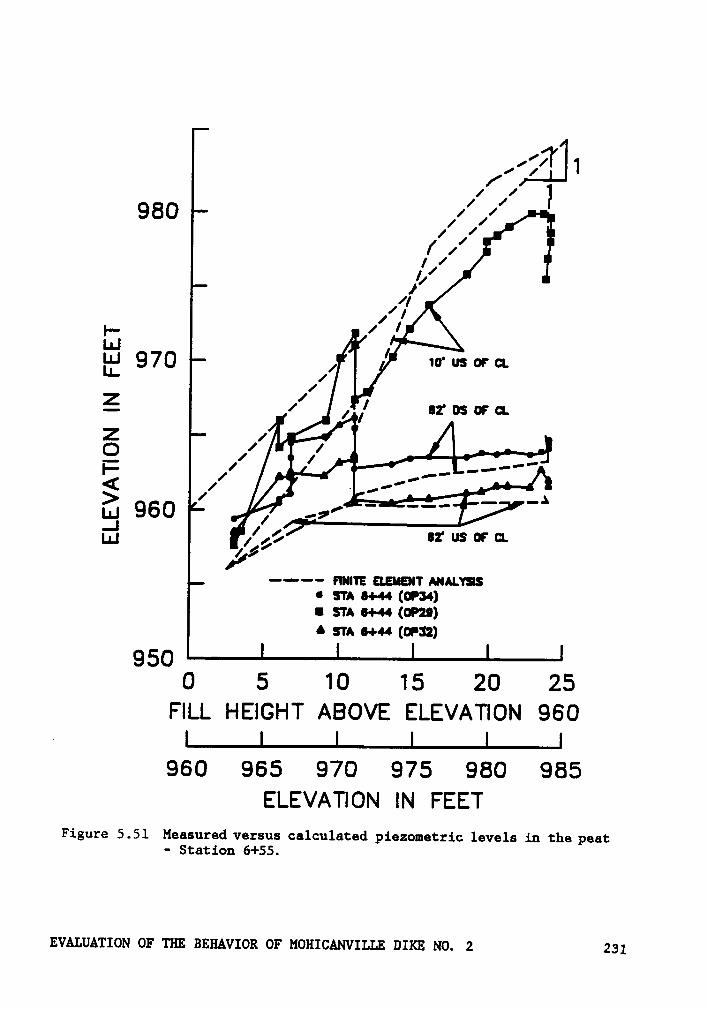
,4:1 I1/1//1 }980 /1 ,1
//1//,/”/
I- 1/ 'I
Q7Q I 10* us ur ct
E 1/ , ’/ sz· ns or crZ 1Q 1/
../ J1
L1_| QÖÜ /„2’ _ -—_
Ü /:49 02* us 0+* CL,9/-··—· FINITE ELEIIENT ANALYSS•
STA 8+44 ($34)¤ su 8+44 (IIP28)6 su 0+44 (01-:2)
950O 5 1 0 1 5 20 25
FILL HEIGHT ABOVE ELEVATION 960
1960 965 970 975 980 985ELEVATION IN FEET
Figure 5.51 Measured versus calculated piezometric levels in the peat- Station 6+55.
zvgwmou or um BEHAVIOR or Mouxcmvxmz um No. 2 231
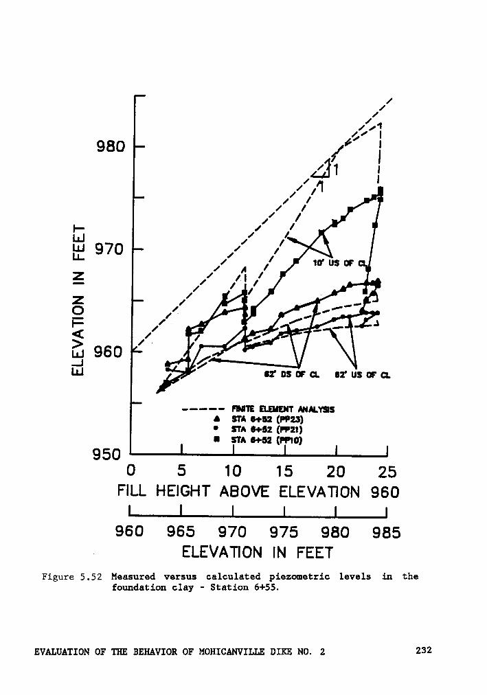
/////11¢’ I980 iA31 I
//gg970 ,»’1/ ..1 A /
E 1/ "1/
z, I
/{/g-/ . „ ___ A
<// r
g ‘ .->
’'u.1960 Y-• fLIJ
g 82'0$Wd. 82'U$WCI.
----- mm mm mussA STA 8+52 (PP23)•
STA 8+52 (R21)• STA •+s2(H•1¤)950
0 5 10 15 20 25FILL HEIGHT ABOVE ELEVATION 960
960 965 970 975 980 9857 ELEVATION IN FEET
Figure 5.52 Measured versus calculated piezometric levels in thefoundation clay - Station 6+55.
EVALUATION OF 'I'IE BEHAVIOR OF MOHICANVILLE DIKE NO. 2 232
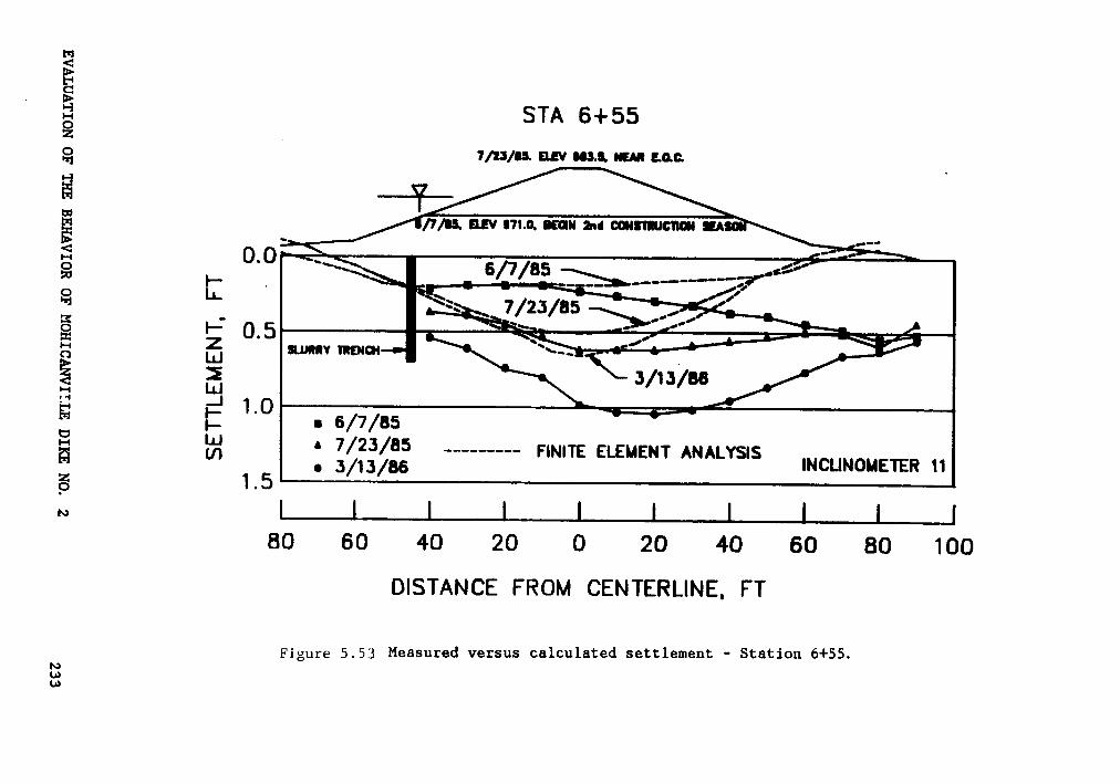
O.
__Q
nzI
·:‘
ä2
I/
2.
ZI2
I2
O2
xx‘°
E,‘I
I'_
gUI
-Ä
XIW
QL
Lä
‘I
\>
*1
a1
.1¢
LJ<
+-1
5I
S5
52
u'
~\
I.1
5Ö
EI
:3I-
•-1Ü
5\
zN
|..1JÜ
xn•
"’E
I"3}
IOä
„E
-¤+
4•
1W
°’Q
+-¤ID
§Ä
°LU
Q3
*2
I'=
z2
<g
;E
Q·—•
IE2
<Ä
"““
==3
Ä5
QI
I¤
'J-2
IL
1.]··
EI5
2I
Ä·
O55
EQ
Mq-
tnä
InU
E¤1
F7gr)
rwQ
Q<
°“¢
01~
rs‘°
“^
I1
IäDO
.l
Öä
Q—
IQo
xnm
c:ca
AA
.L.·.I°.LN3W
3"IJ..I.3S
1avALuA1·1oNorum
ßzxuxvxoaorMOHICANVILLE
Dm: No.
2233
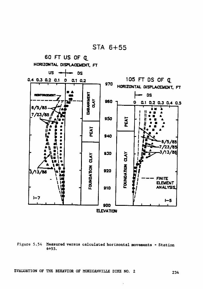
STA 6+5560 FT US OF Q
HORIZONTAL DISPLACEHENT, FT
US •-{-•· DS0.4 0.: 0.2 0.1 0 0.1 0.2 970 105 FT 05 UF (L
HORIZONTAL DISPLACEIAEINT, FT
mummmn I" US°°”°'"ZT gg ä 950 0 0.1 0.2 0.3 0.4 0.55/5/B5 « [A gg
I"
•I AB
•Q A
I II • Q AIl‘ .•
=
I•
. Ü$7]* •* I2 1 11 { { {‘° "
11• Q AII: : Ü 1 A•
I·
5 5 B5tk {Ix:
{ $7/23/B>_1:1:
°I Ü‘ \'*° z 5 .:/1:/06 °2° E {_ \ ¤ Q runat:
11 ä 3 1 1 ctsusur\ 1.. 010 '·· 1
^“^1-*51\I I\1*7 I 1 1-6
900ELEVATION
Figure 5.54 Measured versus calculated horizontal movements · Station‘ 6+55.
EvALUA'1‘i0N or THE BEHAVIOR OF MOHICANVILLE DIKE No. 2 23;,
5.7.3 Analyses of Station 9+00
The two layers of reinforcing placed at Station 9+00 provide an op-
portunity to evaluate the analytical method when applied to multilayer
reinforcement. The foundation conditions at Station 9+00 are shown in
Figure 5.16, and the effects of the previous failures in the upstream area
are evident. No attempt to model the upstream part was made owing to its
complexity. The downstream portion was analyzed using the mesh shown in
Figure 5.55.
Calculated and measured reinforcement forces at the centerline are
shown in Figure 5.56. Between points A and B in Figure 5.56, which covers
the period from August to November, 1984, the calculated results over-
predict the measured forces by a considerable amount and this trend con-
tinues between points B and C, representing the first month of the second
construction season. At point C, a considerable increase in reinforcement
force occurred during nine-day work shutdown in July. As mentioned pre-
viously, this is attributed to creep in the foundation soils and was not
modelled in the analysis. It can be seen that the calculated and measured
values agree well in two respects: One is the decrease in reinforcing
force during the shutdown period (point B), and during the period fol-
lowing construction (point D). The second is the tendency for the upper
layer of reinforcing to be less effective than the lower layer, and for
the force in the upper layer to decrease at a faster rate than that in
the lower layer.
EVALUATION OF THE BEHAVIOR OF MOHICANVILLE DIKE NO. 2 235
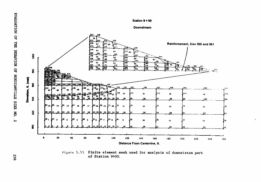
-5-
.‘·"
0O
N
ÜI
52
(TS
Fé
EELg
Ü·=·
.2.
{2
8.I
6zu
Iru
JE
35
‘”=*
g-:
Z:
QE
§/
12
22
3.2
r-8
IE
"I.
”2„
,„E
E-05
•2
2·
>‘,·s
"(
-S
TSz
=-=.·
8E
z=¤
+2
/222-2-
22
„c
8O
cQ
Z‘*·•
S-?
„—
—·
E·¤
28
=~
~ =·2
-=2
5”
2.2
_;-7.
‘Q
-S
m1
_ä
2.
~~
«••-
~~
24.)
55*
:E
ä¤
Iää
äü
52r
-0-
••Q
Q-
°Ü
Üä
2-.:
-2•:~
:.-z9
-°
+·•-·O
OG
—rE
I
—2
jS
LMH
EE
E55LN
ÄIEEQEE5
52
3.5
2-IEEQEE
55**5”‘5’**$S
ä§Kme
ouam
0h6nes
ausI••¤¤)·u‘¤o•••^••a
_
EVALUATIONOF
THEBEHAVIOR
OFMOHICANVILLE
DIKENO.
2236
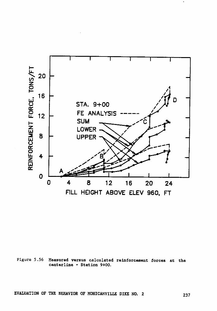
Eä 20ä 4I- /. 16 1Lu 1 Dg STA. 9+00 /1E 12 FEANALYSISI.,
C ’
5 1.0wERB UPPER \ ,
/Üj
Li°‘
A /5O0
4 B 12 16 20 24FILL HEIGHT ABOVE ELEV 960, FT
Figure 5.56 Measured versus calculated reinforcement forces at thecenterline - Station 9+00.
EvALuA·1*1oN or um ßEHAv10R or MOH1cANv1LLE DIKE No. 2 237
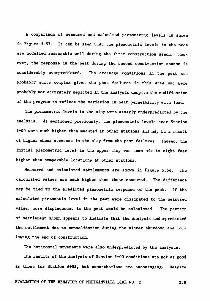
A comparison of measured and calculted piezometric levels is shown
in Figure 5.57. It can be seen that the piezometric levels in the peat
are modelled reasonable well during the first construction seaon. How-
ever, the response in the peat during the second construction season is
considerably overpredicted. The drainage conditions in the peat are
probably quite complex given the past failures in this area and were
probably not accurately depicted in the analysis despite the modification
of the program to reflect the variation in peat permeability with load.
The piezometric levels in the clay were severly underpredicted by the
analysis. As mentioned previously, the piezometric levels near Station
9+00 were much higher than meaured at other stations and may be a result
of higher shear stresses in the clay from the past failures. Indeed, the
initial piezometric level in the upper clay was some six to eight feet
higher than comparable locations at other stations.
Measured and calculated settlements are shown in Figure 5.58. The
calculated values are much higher than those measured. The difference
may be tied to the predicted piezometric response of the peat. If the
calculated piezometic level in the peat were dissipated to the measured
value, more displacement in the peat would be calculated. The pattern
of settlement shown appears to indicate that the analysis underpredicted
the settlement due to consolidation during the winter shutdown and fol-
lowing the end of construction.
The horizontal movements were also underpredicted by the analysis.
The results of the analysis of Station 9+00 conditions are not as good
as those for Station 6+55, but none-the-less are encouraging. Despite
EVALUATION OF THE BEHAVIOR OF MOHICANVILLE DIKE NO. 2 238
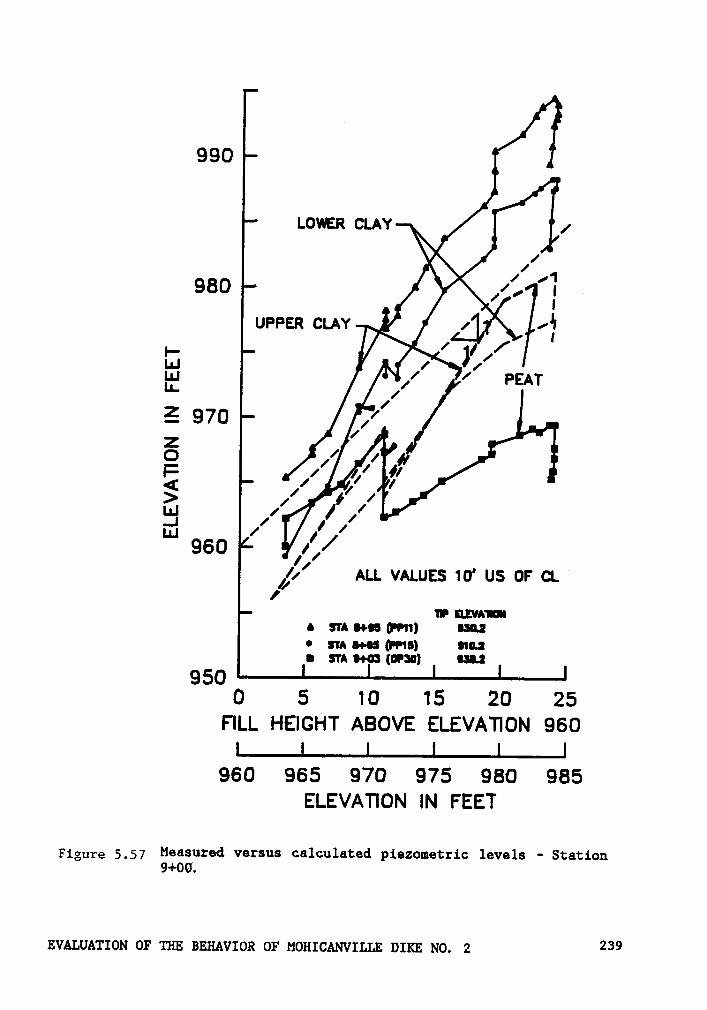
990
LOWERCLAY980
,/1 ’I
u¤=:=6¤ cuw [ Z4:I1 , ,[ ” §1/
PEAT[
E 970 /
6 / ’ 2I: //
/ if( // F / /> ; Ö /uJ x / /fl
//960 /[,/ALL VALUES 10' Us OF ct. E
[
'IP EIVAÄ•STA •+•¤ (,I•••11)
uu.:• sm •«•-•s (uns) uu• m •+¤¤:¤:·¤:n uu950
0 5 10 15 20 25FILL HEIGHT ABOVE ELEVATION 960
960 965 970 975 980 985ELEVATION IN FEET
Figure 5,57 Measured versus calculated piezometric levels - Station9+00.
EVALUATION or um ßmmvxox OF Mo1ucANv1LLE num No. 2 239
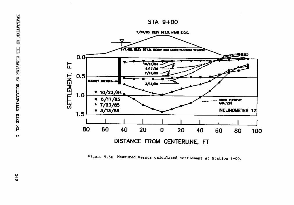
09
9lll
1ill
N,_
EO
_S
QS
\Ä
N‘
E; ö'§
~„E
EG
1->
1N
1‘°
§1
'
H{J
_bx
EO
L1.°
·\x\
,,._
E_
\\\LuZ
4)
2E
l‘x\Q
1S
1 1O
Üä
CJä
El \1
Nl'
'¤‘
a1O
ä\
E1;
g'¥
{lv
ll
Q*;
§E
11
1O
E2
<<¤
szE
.äää
ä2
1E
2"··**
0“-
2ä
s‘“
2i
?»:*1
<°
•—ä
*In
gn¢
Q$1:)
°Q
uS
Q
'°äZ
<Q
<°
«<b
I ••QQ
0ID
°°0
0.4
.41
id‘J.N
3N3'|J.L3S
EVALUATIONor
umBEHAVIOR
orMOHICANVILLE
numNo.
z2;,0
extreme simplification of complex soil conditions, the analysis reflected
similar trends as the measured data. In particular, the fraction of the
total reinforcement force carried by each layer was modelled well pro-
viding encouragement for the use of finite element techniques for multi-
layered reinforced systems.
5.8 Study of Ageing Effects on Compacted Clay
When construction resumed in the spring of 1985, the rate of increase
of load pickup in the reinforcement was smaller than it had been during
the previous fall. This phenomenon was further highlighted when the fi-
nite element analysis showed that a greater rate of load increase would
be expected. In attempting to explain this phenomenon, the possibility
that the fill stiffened with time was hypothesized. This section will
discuss the effects of ageing on the properties compacted soils, and
discuss a laboratory test program conducted to measure these effects for
the Mohicanville Dike No. 2 fill.
Previous studies of ageing effects on the strength and stiffness of
compacted soils have been performed by Seed and Chan (1957), Trollope and
Chan (1960), Seed, Mitchell and Chan (1960) and Casagrande, Hirschfeld
and Poulos (1963). These studies showed that an increase in stiffness
and strength of compacted clays can occur with time after compaction.
The changes in behavior are often attributed to thixotropic effects,
whereby property changes occur with time due to such factors as changes
EVALUATION OF THE BEHAVIOR OF MOHICANVILLE DIKE NO. 2 241
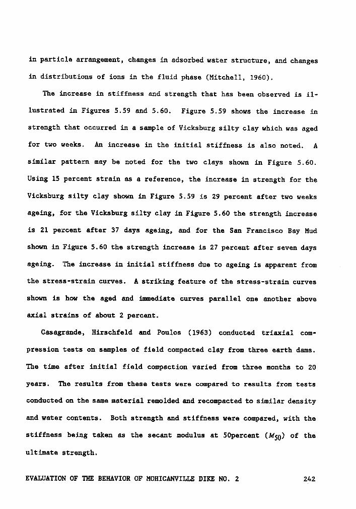
in particle arrangement, changes in adsorbed water structure, and changes
in distributions of ions in the fluid phase (Mitchell, 1960).
The increase in stiffness and strength that has been observed is il-
lustrated in Figures 5.59 and 5.60. Figure 5.59 shows the increase in
strength that occurred in a sample of Vicksburg silty clay which was aged
for two weeks. An increase in the initial stiffness is also noted. A
similar pattern may be noted for the two clays shown in Figure 5.60.
Using 15 percent strain as a reference, the increase in strength for the
Vicksburg silty clay shown in Figure 5.59 is 29 percent after two weeks
ageing, for the Vicksburg silty clay in Figure 5.60 the strength increase
is 21 percent after 37 days ageing, and for the San Francisco Bay Mud
shown in Figure 5.60 the strength increase is 27 percent after seven days
ageing. The increase in initial stiffness due to ageing is apparent from
the stress-strain curves. A striking feature of the stress-strain curves
shown is how the aged and imediate curves parallel one another above
axial strains of about 2 percent.
Casagrande, Hirschfeld and Poulos (1963) conducted triaxial com-
pression tests on samples of field compacted clay from three earth dams.
The time after initial field compaction varied from three months to 20
years. The results from these tests were compared to results from tests
conducted on the same material remolded and recompacted to similar density
and water contents. Both strength and stiffness were compared, with the
stiffness being taken as the secant modulus at 50percent (Mgo) of the
ultimate strength.
EVALUATION OF THE BEHAVIOR OF MOHICANVILLE DIKE NO. 2 242
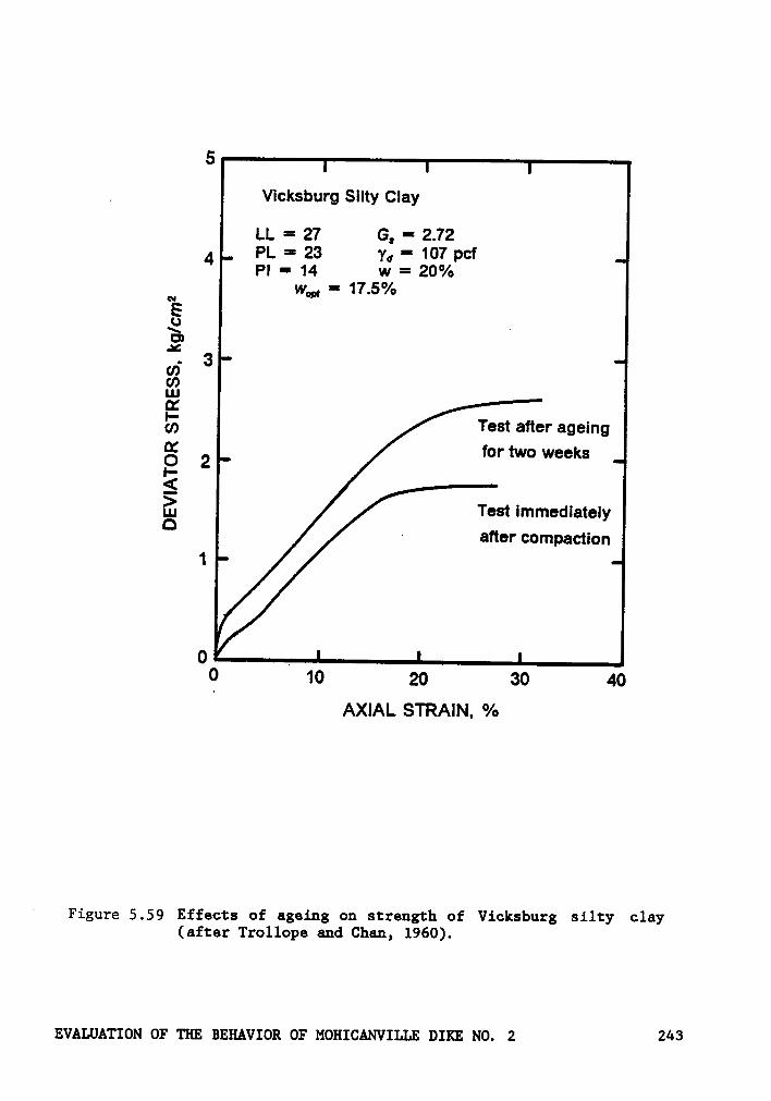
5
. Vicksburg Silty Clay
LL = 27 G, = 2.724 PL = 23 Yu = 107 pcf
Pl = 14 w = 20%N w„, == 17.5%E3 .ca“
605U)LuM
Test after ageingg 2 for two weeksI-S
Test immediately· after compaction
1
0 .0 10 20 30 40
AXIAL STRAIN. %
‘Figure 5.59 Effects of ageing on strength of Vicksburg silty clay
(after Trollope and Chan, 1960).
EVALUATION OF THE BEHAVIOR OF MOHICANVILLE DIKE NO. 2 243
40
IIIIIEEIJI ···“i < IFF;-="==¤¤¤g, EEEIIIE ;· y- —*-—=-QQ4! !!¤¤z Q]-..[j-1 FAIIIIIIIII
'°
-
·. . . . ._—''*••·;„¤-.1;.:;:% H-•-JI;-¢‘=-'—'=¤¤I
IEI;·__IIIIIIIIXIIII!Il-ggEgiäänl
IIIQQIE FIIAIEIIEIIIIIII·r 'I ·
‘·IIIIIIIIE III···-···-··—·-·99 • 9 L4.; n an 0 u 0 9 • 0 I I I I
Figure 5.60 Effects of ageing on strength and pore water pressure ofVicksburg silty clay and San Francisco Bay Mud (afterSeed, Mitchell and Chan, 1960).
EVALUATION OF ’I'HE BEHAVIOR OF MOHICANVILLE DIE NO. 244
For Canyon Dam clay, a medium plastic silty clay, undisturbed block
samples were obtained three months after field compaction.
Unconsolidated-undrained (UU) triaxial tests showed the undisturbed sam-
ples to have M50 values of about three times the M50 values of the lab
compacted values and strengths about 30 percent greater. In
consolidated-undrained (CU) tests the consolidation pressure appeared to
have an effect on the ratios of NQ0, with a ratio of three at low con-
solidation pressures (less than 2 kg/cm2) and a ratio nearing one as the
consolidation pressure increased above 4 kg/cm2. Strengths based on the
CU tests were about equal over the entire range of consolidation pres-
sures.
For Arkabutla Dam clay, a medium plastic silty clay, undisturbed
samples were tested 18 years after field compaction. Comparing these test
results with those from tests on freshly compacted samples, the undis-
turbed and the freshly recompacted values of M50 and strength were about
equal for UU tests. In CU tests, the strengths were nearly the same, but
the values of bqm for the undisturbed samples were 1.1 to 1.9 times those
for the freshly compacted samples.
Similar comparisons for sandy clay from the Conchas Dam, tested 20
years after field compaction, showed M50 values three times greater UU
test on undisturbed samples than for freshly recompacted samples. In
these UU tests the strengths were about the same. In CU tests practically
no differences were discerned in either strength or M50, values except
at very low consolidation pressures where the hqw ratio approached a value
of two.
EVALUATION OF THE BEHAVIOR OF MOHICANVILLE DIKE NO. 2 245
An interesting point concerning the above tests is that all, except
those on the Conchas Dam fill, were performed on soil at moisture contents
at optimum or higher.
The above discussion demonstrates that the strength and stiffness of
compacted soils increase with time, and that the amount of increase varies
from soil to soil. The effect of ageing on the strength and stiffness
properties of the fill material at Mohicanville Dike No. 2 was assessed
through a laboratory investigation using unconsolidated-undrained tests
on compacted samples. Based on the results of these tests, the effects
of ageing were included in finite element analyses by increasing the
strength and stiffness of the fill between the end of the first con-
struction season winter shutdown and the beginning of the second. The
results of these studies are described below.
5.8.1 Soil Properties
A 150 lb sample of the embankment fill material was obtained from the
Huntington District Corps of Engineers. Soil classification, grain-size,
water content-density relations, and unconsolidated-undrained (UU)
triaxial compression tests were performed on the soil.
The material grades as a gravelly sandy clay, classified as a CL in
the Unified Soil Classification System. The clay has a liquid limit of
31, a plastic limit of 17 and a plasticity index of 14, determined in
accordance with American Society for Testing and Materials (ASTM) Stand- d
ards D-4318 and ASTM D-2217. The specific gravity was determined to be
EVALUATION OF THE BEHAVIOR OF MOHICANVILLE DIKE NO. 2 246
2.74 in accordance with ASTM D·854. The grain size distribution, deter-
mined in accordance with ASTM D·422, is shown in Figure 5.61. Also
plotted in Figure 5.61 are the limits of grain size determined for the
borrow materials at the site by Law Engineering Testing Company (Collins
et al. 1982). The material used in this study is near the fine side of
the borrow material identified at the site.
Standard compaction water content-density relations for the fill were
determined in accordance with ASTM D·698 and are shown in Figure 5.62.
The maximum dry density is 119.0 pcf at an optimum moisture content of
14.5 per cent. Also shown on this figure are the results of compacting
the soil in a Harvard Miniature Compaction Apparatus (Wilson, 1970) at
various water contents. The results plotted here are for compaction in
the Harvard Miniature device using five layers and 25 tamps/layer, with
a 40 lb spring. This combination of tamps and layers was used to mold
the UU test specimens.
The natural moisture contest of the soil as delivered to Virginia Tech
was 15.4 per cent. This moisture content is about 1 per cent above op-
timum. This being the case, the test specimens were molded using the soil
as received after removing the material larger than the #4 sieve size (4.7
mm). Based on the results shown in Figure 5.62, it was expected that this
would provide test specimens at an approximate dry density of 118.2 pcf
when compacted in the Harvard Miniature apparatus. After compacting, the
specimens were placed between two lucite end caps, encased in two latex
membranes and sealed at each end with two O-rings. Silicon grease was
EVALUATION OF THE BEHAVIOR OF MOHICANVILLE DIKE NO. 2 247
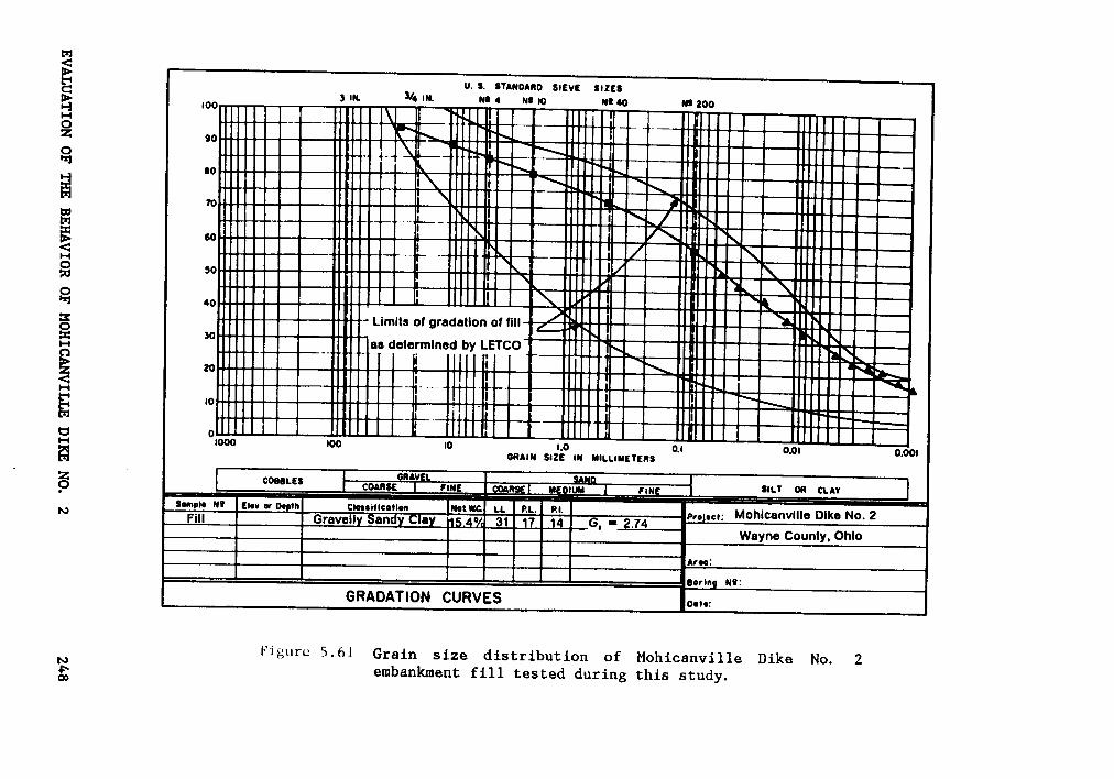
6Ä
I.
IIIIIIIIIIIIIIIMIIII
IIIIIIIIIIIIIIIHIIIII
Ü2
NIIIIIIIIIIIIIIZ
IIIH
IZ
5—
——
——
—_
——
——
——
H|’.l—
——
II—ÄQ
.6
==
==
==
==
==
==
:::==
=!:=
°·E
Zää
IIIIIIIIIl|„A
Ä2
'IHIIIIV
IIE
°IIIIIIIIB
IIIIIIIV
III§
S~—
6IIIIIIIH
IIHIIIII
nl!
*S
—·-
——
_—
——
DZ
—K
_—
——
——
I1—
_—
ÄE
•Q
qTi
>5
2=======g!2=======!2gg=Ä .;=
2¤ ·»
5=2===ää?2=======V====EÄ
vzIIIIl|•A
IIIIIIIlIIII2-
„IIIIIIHIE
IIIIIIIIIII§
*Z
Ä;.3
IIIIAIQ
IIIBIIIIIA
IIIII2
«“a.*3
g{E
äiü
iuä
ää
äiiä
ää
iiiää
äg'
_G
-s-«
Ҥ
==
!:=2
==
==
==
=ä
==
==
==
„1
22;2
ÄEEIIII“
..IIHIU
IIIIIIMIIIIIIIE
ÄIN
II‘
anÄ
°··
‘·•-
IIIHIIIIIIII
_;¤IIII
ä°+,§“
nnnunuuunzun6
.*2nun:
.„2.;;
„Q
EIQ
EZ
SZ
ZQ
ZE
E°
EE
QE
Ä.
W°¤
>~Ä
Z9
Q
llllälllllll ä
ll!-·
=”’ä
E2
2‘ö
6---O
:1cs
'r
V2
_2
—* Q
IQG
IIIIIIII2;-2
IIII5;
IIIIIIII-
,,IIII
.Ä,2
._„..,—
—_—
——
_——
——
—·‘
¤—
——
_E
,==
==
==
ä=
==
=--2
::::2
,,..
;:::::::::::::::=::::8
22
——
—·—
——
——
——
—*-*—
*——
—-
Ä2
2O
IIIIIIIIIIIIIIIIIIII„
ÄIIIIIIIIIIIIIIIIIIIIä 2;
6Ä.
—-—
--W-----_°°
§§
EVALUATIONormz
mmvxoxorMouxcmvxnm
numNo.
2266
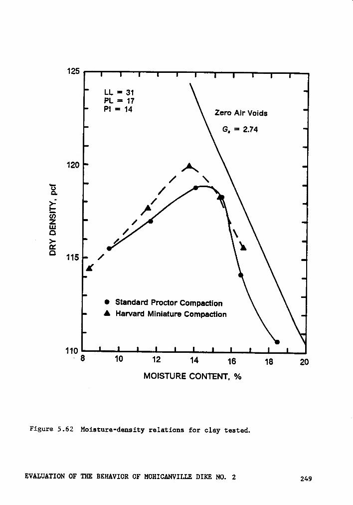
125
LL = 31PL = 17P! = 14 Zero Air Voids
G, = 2.74
120 A
ä />; /1-ä ß
0 / \E
’x
° 115 xK
•Standard Proctor Compaction
A Harvard Miniature Compaction
Y110
= 8 10 12 14 16 18 20MOISTURE CONTENT, %
Figure 5.62 Moisture-density relations for clay tested.
EvALuA'r1oN or um Bmmvxou or 1~1oH1cANv1LLE Dm: No. 2 2l*Q
placed between the membranes on test specimens which were to "age" to
inhibit leakage and the samples were stored under water until tested.
The data in Table 5.6 show that the target dry density of 118.2 pcf
was not met in all the specimens. These data also show that an increase
in moisture content occurred as the time of storage increased. This ap-
pears to indicate that leakage of water into the soil specimens occurred
despite the precautions taken. Two of the 4-week test specimens had water
contests high enough to make the samples noticeably soft when removed from
the water storage tank. These samples showed such low strengths in
testing that the results were discarded.
The effect of ageing on fill properties was assessed by performing
UU triaxial tests on soil samples immediately following compaction and
on samples that were allowed to age for periods of 1, 2 and 4 weeks fol-
lowing compaction. The UU tests were performed in accordance with ASTM
D2850. At each time four UU tests were conducted using confining pres-
sures of 0.25, 0.50, 075 and 1.00 tsf. The stress-strain curves from
these tests are shown in Figures 5.63 through 5.66. The results from two
of the 4·week samples were disregarded due to an unusually high water
content after testing, indicating leakage occurred during storage. The
stress-strain curves exhibit behavior similar to the behavior of the
Vicksburg silty clay discussed earlier: an initial stiff response fol-
lowed by a relatively linear increase in strength. Table 5.7 shows the
strengths interpreted from the tests based on failure at 15 percent
strain. An increase in strength occurs for samples tested after 1-week
of ageing. However, samples tested 2- and 4-weeks after molding, in
EVALUATION OF THE BEHAVIOR OF MOHICANVILLE DIKE NO. 2 250
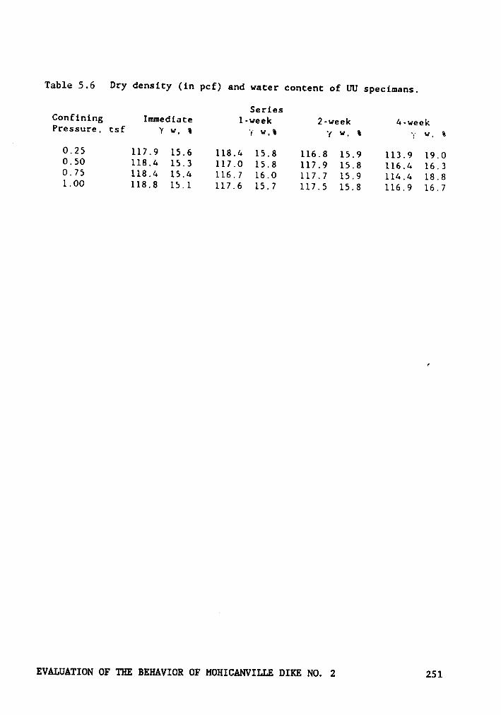
Table 5,6 Dry density (in pcf) and wacer concenc of UU specimans.
SeriesConfining Immediace 1-week 2-week 4-weekPressure, csf Y w, S Y w,S ·y w, S —. w, S
0.25 117.9 15.6 118.4 15.8 116.8 15.9 113.9 19.00.50 118.4 15.3 117.0 15.8 117.9 15.8 116.4 16.30.75 118.4 15.4 116.7 16.0 117.7 15.9 114.4 18.81.00 118.8 15.1 117.6 15.7 117.5 15.8 116.9 16.7
EVALUATION OF THE BEHAVIOR OF MOHICANVILLE DIKE NO. 2 251
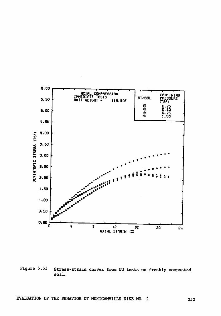
6.00Hx1HL COHPBESSION co FI 1 6IHHEDIRTE TESTS STM6¤L PBgSS¤Rg5.50 UNIT HEIGHT ¤ 1l8.BOF (TSF)
3 8‘§ä6.00 A 0I7so 1.004.50
;_· 4.00vs‘:.,, 3.50uuFE • • ‘@,7, 6.00 _ , . •
° °2 • • °52.60 ,•° _,¤••°°
Ö••
·
I g··· .•° e Q Q — ¤ •,7, 2.00 .•E g ! ·D
•°1.60 _•°„„·:..•’• lu ·l•°;”¤ n'. V
1.00 ¤"' ,•'n‘ •B.-
••••
0.60,:_,•°
sp0.00
0 4 a I2 I6 20 24HXIRL STRRIN 121
Figure 5-63 Stress·straiu curves from UU tests ou freshly compactedsoil.
EVALUATION OF THE BEHAVIOR OF MOHICANVILLE DIKE NO. 2 252
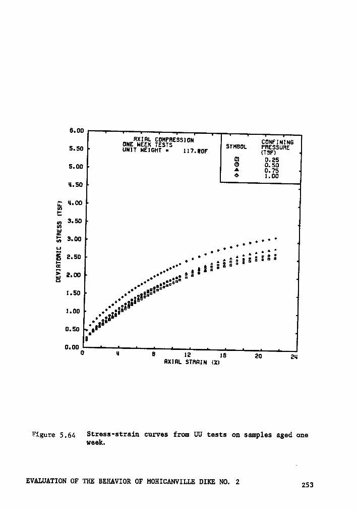
6.00HXIHL CUHPBESSION CONFININGONE HEEK TESTS STHBUL PHESSUBE5.50 UNIT HEIGHT ¤ 117.BOF (T3F]
8 8*ää*6.00 A 0:750 1.00
4.50
Q 4.00th2:
3.50• •
°• • • Q•
O°
• •
‘ ‘ ‘ A:52.60·-
•O•
8 3=
¤I
{J 2.00 •,•° H.: .1 *O• nlgul
•••
02;:ß1.00 .•° ;§a°°
• I0.50 38l
0.000 4 8 12 18 20 24
FIXIRL STRHIN (Z)
Figure S_64 St1'6SS'St1.'&iI1 CUIVB8 fIOl¤ UU 1288125 OR S8Il1pI.BS 8gBd 0116week.
EVALUATION OF TIE BEHAVIOR OF MOHICANVILLE DIKE NO. 2 253
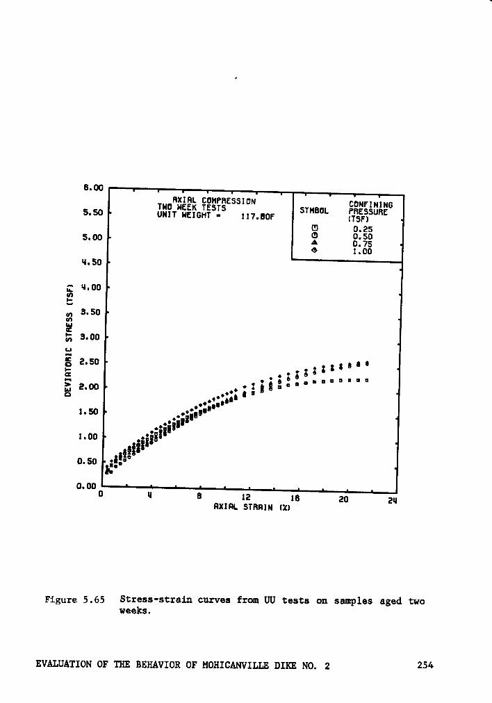
6.00HXIHL CUHPBESSION CQNF]N]NgTun HEEK Tcsrs5.50 um? HEIGHT - ll7.BOF STHBUL Ggäsunf
E2 3·§ä5·°° A 0Ivs¢ 1.00ql
gg Q.00IhZ':„, 3.50IhInlE?,,, 5.00E!
• V : 0u J „ M I E B•
¤ ¤'> 2.00 •
·g 2 ¤
I1.50__.;§••'
• I1.00 vg;1%=*gig;0.500.00
0 M 6 I2 IB 20 2Mnxxm. smmu 121
F1 ure 5,65 Stress-strain curves from UU tests ou samples aged two8weeks.
EVALUATION OF TIE BEHAVIOR OF MOHICANVILLE DIKE NO. 2 254

6.00HXIHL COHPRESSION CONFININGFOUR HEEK TESTS S B5.50 UNIT HEIGHT •
116. FOFTH OL FI%EF%SURE
Ü 0. 505.00 0 1.00
ul
; 4.00vb*:
th1.1..1E2§ 2.50 O °0E.
l·
B g { : ¤ u u2.00U
_, •
nl T
1.50 .••'°°.•'°··
Is1.00 .-'°•'°
n'.0.500.00
0 U 8 12 15 20 2\1|RXIRL STRHIN [Z]
Figure 5.66 Stress-strain curves from UU tests on samples aged fourweeks.
EVALUATION OF THE BEHAVIOR OF MOHICANVILLE DIKE NO. 2 255
general, show slight reduction in strength. The differences in strength
may be attributable to differences in molding density and water content.
The data in Table 5.6 show that the samples tested immediately after
molding had the highest average density of all the samples tested.
The stiffness of each sample was characterized in two ways. Table
5.8 shows the initial stiffness determined using standard hyperbolic soil
model techniques (Duncan et al. 1980) and normalized by atmospheric
pressure. Table 5.9 shows the secant modulus of each sample at a stress
level of 0.4 tsf corresponding to an average embankment pressure at the
level of the reinforcement. The trends shown in these two tables are
similar to the trends of the strength data. A general increase in
stiffness with time can be seen, but significant scatter in the results
is evident.
Despite the scatter in the results, it is clear that some gain in
strength and stiffness does occur with ageing in the clay from
Mohicanville Dike No. 2. Based on the results of the laboratory tests,
it was concluded that a reasonable estimate of the effects of ageing be-
tween the first and second construction season would be a ten percent
increase in strength, and a 100 percent increase in modulus.
5.8.2 Finite Element Analyses
A finite element analysis to investigate the effects of ageing was
performed using the mesh and profile used for previous analyses of Section
6+55. The analysis was performed by simulating the first construction
EVALUATION OF THE BEHAVIOR OF MOHICANVILLE DIKE NO. 2 256
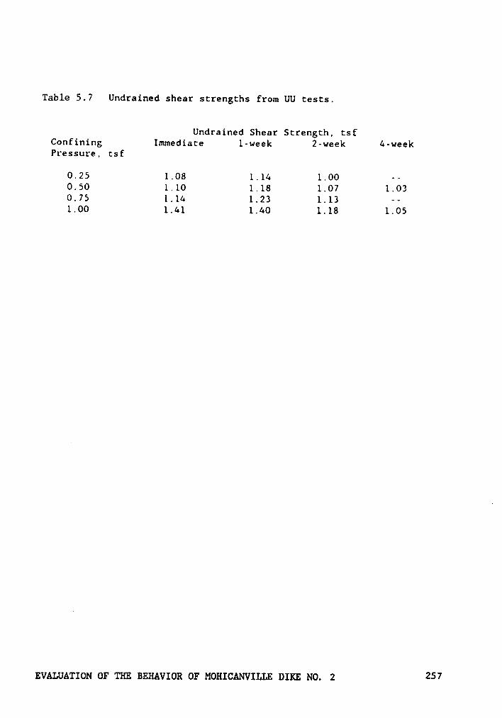
Table 5.7 Undrained shear strengths from UU tests.
Undrained Shear Strength, tsfConfining Immediate 1-week 2-week A-weekPressure, tsf
0.25 1.08 1.1& 1.00 --0.50 1.10 1.18 1.07 1.030.75 1.1A 1.23 1.13 --1.00 1.&1 1.&0 1.18 1.05
EVALUATION OF THE BEHAVIOR OF MOHICANVILLE DIKE NO. 2 257
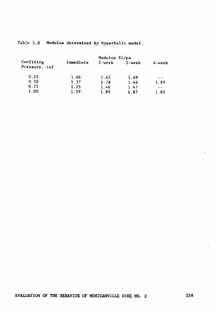
Table 5,8 Modulus decermined by hyperbolic model.
Modulus Ei/paConfining Immediate 1-week 2~week 6-weekPressure, csf
0.25 1.66 1.65 1.69 --0.50 1.37 1.78 1.66 1.890.75 1.25 1.66 1.67 -·1.00 1.59 1.89 1.87 1.85
EVALUATION OF THE BEHAVIOR OF MOHICANVILLE DIKE NO. 2 258

Table 5,9 Secant modulus at 800 psf shear strength.
Modulus, psfConfining Immediate 1—week 2-week A-weekPressure, tsf
0.25 37.7 A1,7 66.7 --0.50 22.7 &7.6 3&.5 57.10.75 22.7 62.5 57.1 -·1.00 47.6 166.7 100. 133.
EVALUATION OF THE BEHAVIOR OF MOHICANVILLE DIKE NO. 2 259
season and the winter shutdown as before, and increasing the stiffness
and strength of the new fill at the start of the second construction
season. The strength of the fill was increased by ten percent and the
stiffness was increased by a factor of two as compared to the initial
stiffness. The calculated centerline reinforcement force is shown as the
dashed line in Figure 5.67. There was little change from the previous
results indicating stiffening of the new fill had little effect on the
reinforcement forces. The calculated in settlements and pore water
pressures were slightly smaller than those calculated in the analyses
described previously. No discernible changes in the horizontal movements
were noted. During the consolidation phase of the analysis, no increases
in fill strength occurred, while the strength of the peat and soft clay
increased by one·half to one and one-half percent.
A second analysis was performed in which the strength and stiffness
of the old fill material was raised at the beginning of the second con-
struction season by the same ratios as the new fill. The effect of
"ageing" both the old and new fill is shown on Figure 5.67 by the solid
line. It can be seen that this change had the effect of reducing the
reinforcement force and provides results in excellent agreement with the
measured data. Ageing both fills reduced the settlement at the re-
inforcement level and reduced the lateral movements at the toe. However,
there was little change in settlements in the peat and soft clay compared
to the unstiffened analyses. In this analysis the shear stress levels
in the old fill were markedly higher indicating more load being carried
EVALUATION OF THE BEHAVIOR OF MOHICANVILLE DIKE NO. 2 260
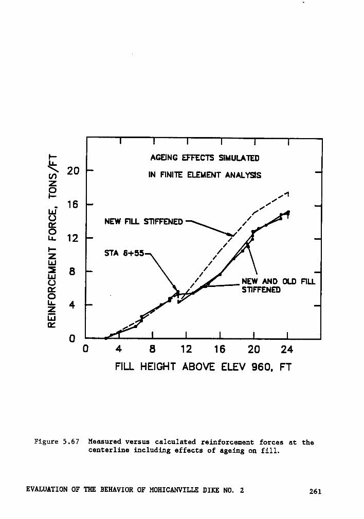
AGEING EFFECTS SIMULATEDä 20 IN FINITE ELEMENT ANALYSISZE ,/4
• [ZLIJ / ~ät) NEW FILL STIFFENED ;/ /
OLn 12 1 1•- 4 /Z su 6+ss / „I.|J //E B 1O // NEW AND OLD FILLQ: STIFFENED
2 4 .2LU
O .4
0 4 8 12 16 20 24FILL HEIGHT ABOVE ELEV 960. FT
Figure 5.67 Measured versus calculated reinforcement forces at thecenterline including effects of ageing on fill.
EVALUATION OF THE BEHAVIOR OF MOHICANVILLE DIKE NO. 2 261
by the fill. The shear stress levels in the peat and soft clay were lower
than those calculated in the unstiffened analyses.
From the analyses discussed above, it appears that ageing of the new
fill did not materially affect the reinforcement forces. Further, there
would seem to be little reason to suspect that ageing of the old fill
resulted in the lower measured forces, because this fill had been in place
some 45 years. The mechanism causing the gain in strength might be
strength gain in the foundation soils due to secondary compression ef-
fects.
5.9 Summary and Gonclusions
The experience gained from design, construction, instrumentation, and
analysis of Mohicanville dike has provided information of considerable
value with regard to the behavior of reinforced embankments on weak peat
and clay foundations.
First, it has been demonstrated that it is feasible to stabilize an
embankment on a weak foundation very effectively using a single layer of
reinforcement near the base of the embankment. This is particularly
valuable in light of the height of the embankment built at this site, some
28 feet above natural ground level. Second, it has been shown that such
an embankment can be adequately designed using limit equilibrium and fi-
nite element techniques. .
The instrumentation studies performed on the embankment during and
following construction have provided very valuable information regarding
EVALUATION OF THE BEHAVIOR OF MOHICANVILLE DIKE NO. 2 262

the accuracy of the finite element analyses and the limit equilibrium
slope stability analyses used to design the embankment. Comparisons of
the calculated and measured reinforcement forces indicate that the finite
element analyses provide an effective means of estimating the amount of
reinforcing force that would develop during construction, and the rate
at which the force would decrease after construction as the foundation
soils consolidate. The measured movements of the embankment have been
quite small, consistent with the expected behavior of an embankment having
a factor of safety equal to 1.3 at the end of construction. Thus the
combination of finite element analyses to estimate reinforcing forces,
and conventional limit equilibrium analyses to calculate factor of safety
appears to provide an effective approach for design of reinforced
embankments on weak foundations.
The study of the effects of ageing of the compacted clay fill were
inconclusive. When only the strength and stiffness of the new fill was
increased during the winter shutdown, the calculated results were changed
very little. When the strength and stiffness of the old fill was in-
creased as well, the results were in excellent agreement with the field
measurements. That the strength of the old fill could actually have in-
crease seems unlikely, given that it had been compacted some 45 years
prior. However, it seems likely that some stiffening of the soils, per-
haps the foundation as well as the embankment soils, did occur over the
winter shutdown, resulting in the changed behavior over this period that
was clearly evident in the measured reinforcement forces during the early
stages of the construction season.
EVALUATION OF THE BEHAVIOR OF MOHICANVILLE DIKE NO. 2 263

CHAPTER VI
ANALYSIS OF ST. ALBAN TEST EMBANKMENTS
6.1 Introduction
In 1984, three instrumented test embankments were constructed to
failure at a site near St. Alban, Quebec, Canada, to study the effect of
geogrid reinforcement on the stability of embankments on a soft sensitive
clay deposit. Two of the embankments were reinforced with Tensar SR-2,
a high strength, high density polyethylene geogrid having uniaxial
strength characteristics. One of these embankments had the geogrid placed
in a flat-lying position and the other had the geogrid placed in an up-
right position to form a geogrid mattress structure. A third embankment,
unreinforced, was constructed as a control.
The primary objective of this chapter is to assess the suitability
of various finite element techniques for the analysis of reinforced
embankments on soft, sensitive clays. This was accomplished by a straight
forward interpretation of the soil data, analyzing the field trials and
comparing the analytical results to the observed behavior. A comprehen-
sive report of the field trials, containing a discussion of the subsurface
exploration, the embankment design, instrumentation, construction, field
measurements and observations was prepared by Busbridge et al. (1985).
A review of certain aspects of this report is presented here as background
to the analyses performed during this study.
ANALYSIS OF ST. ALBAN TEST EMBANKMENTS 264
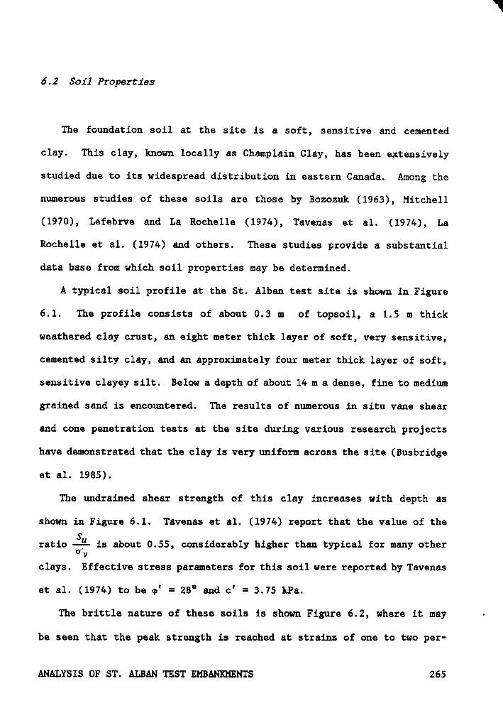
‘l
6.2 Soil Properties
The foundation soil at the site is a soft, sensitive and cemented
clay. This clay, known locally as Champlain Clay, has been extensively
studied due to its widespread distribution in eastern Canada. Among the
numerous studies of these soils are those by Bozozuk (1963), Mitchell
(1970), Lefebrve and La Rochelle (1974), Tavenas et al. (1974), La
Rochelle et al. (1974) and others. These studies provide a substantial
data base from which soil properties may be determined.
A typical soil profile at the St. Alban test site is shown in Figure
6.1. The profile consists of about 0.3 m of topsoil, a 1.5 m thick
weathered clay crust, an eight meter thick layer of soft, very sensitive,
cemented silty clay, and an approximately four meter thick layer of soft,
sensitive clayey silt. Below a depth of about 14 m a dense, fine to medium
grained sand is encountered. The results of numerous in situ vane shear
and cone penetration tests at the site during various research projects
have demonstrated that the clay is very uniform across the site (Busbridge
et al. 1985).
The undrained shear strength of this clay increases with depth as
shown in Figure 6.1. Tavenas et al. (1974) report that the value of the
ratio {äh is about 0.55, considerably higher than typical for many other
clays. Effective stress parameters for this soil were reported by Tavenas
et al. (1974) to be o' = 28° and c' = 3.75 kPa.
The brittle nature of these soils is shown Figure 6.2, where it may ·
be seen that the peak strength is reached at strains of one to two per-
ANALYSIS OF ST. ALBAN TEST EMBANKMENTS 265
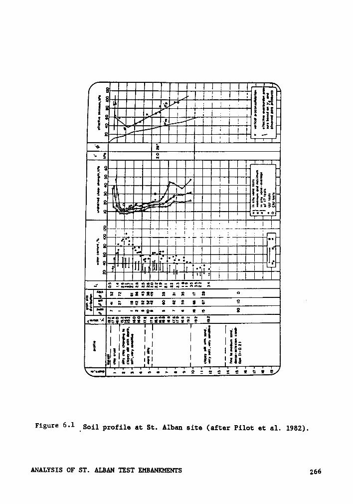
lIlllIIl"\6 IIIIIIIIIIIIÄIII I2;E .IIIlIIllB.§l§I;—IIl!III§§lII . I; IIIQZEHIIIIIIIKIII _ ;
’I
ElllIlIlIlIIIIKL-J» —
2 lIlIllIIlllIllllI""'1IIIIIIIIIIIIIIIII _§; IlllllIlI!!BIIIIllI |
2 IIIlIIIIllllIIIIIHÜ . 22 III[l!I!g§”LI!IIlIIII 2 E 2;5i
ZIIHIIII-I6gg
6 6'TTTTT TTT6 6 I"2 IEIIEIHEIIIIIIIIIIIIIIIWIIIIIHIIIIIIIII -lIIIIIIIIl2 :2.-:.;:2:2:2;::::2::
·~ --u¤g• uv
-
~•2 2 8
•-··~·‘# Eäääéiää E SEZQSEEEE E EI |°¥ ' 6 I Ü IB?I
II ääßI 2- '
I I 2: z=¤I I} I2};
es 222 ·E' .2 *22;Q -«•·••••••·••·<2:¤2zc2:ez
Figure 6·l _Soil profile at St. Alban site (after Pilot et al. 1982).
Amusxs or sr. mm usr EMBANKMENTS 266
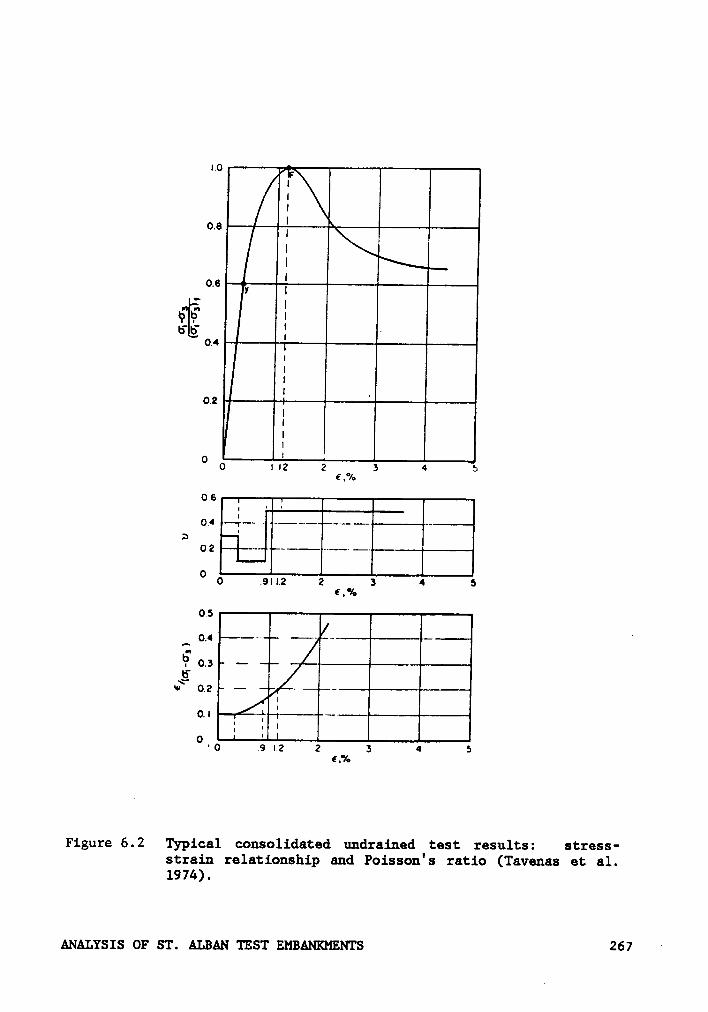
Y YALIIIIII
"~>~§’GF
IIIIIIIIIIO O 1¤2 2 3 4 6
6,%
0.6II-
° O, n
_
0O .9I|.2 2 3 4 5
6,%
0.5
§v\ 0.2
ni ==0 ‘O .9 I.2 2 3 4 5
E,./•
Figure 6.2 Typical consolidated undrained test results: stress-strain relationship and Poisson's ratio (Tavenas et al.1974).
ANALYSIS OF ST. ALBAN TEST EMBANKMENTS 267 ·
cent, and that the shearing resistance decreased rapidly beyond the peak.
Tavenas et al. (1974) reported results of consolidated undrained tests
in which lateral deformations were measured to obtain data on Poisson's
ratio as shown in Figure 6.2. In addition, Tavenas et al. presented the
results of hydraulic fracture tests from which in situ Kb values were
determined.
Consolidation characteristics of this clay reported by Tavenas et al.
(1974) are shown in Figure 6.3. The sharp break in the e versus log p
curve is generally attributed to a structural breakdown which occurs at
a critical pressure and results in a change of fabric of the clay (Quigley
and Thompson, 1966). One-dimensional consolidation tests on undisturbed
sensitive clays are characterized by a break at a pressure believed to
correspond to the preconsolidation pressure, pc. La Rochelle and Lefebrve
(1970) report that this pressure is frequently used in practical design
to determine the maximum load to be applied to the clay without resulting
large settlements.
The soil used for the fill was a uniform, medium to coarse grained
sand containing about ten percent fine sand and ten percent gravel, having
a uniformity coefficient of 3.0 (La Rochelle et al. 1974). The sand was
placed in a loose state with minimal compaction effort. The friction
angle of the sand as placed was estimated to be 34° by Busbridge et al.
(1985).
ANALYSIS OF ST. ALBAN TEST EMBANKMENTS 268
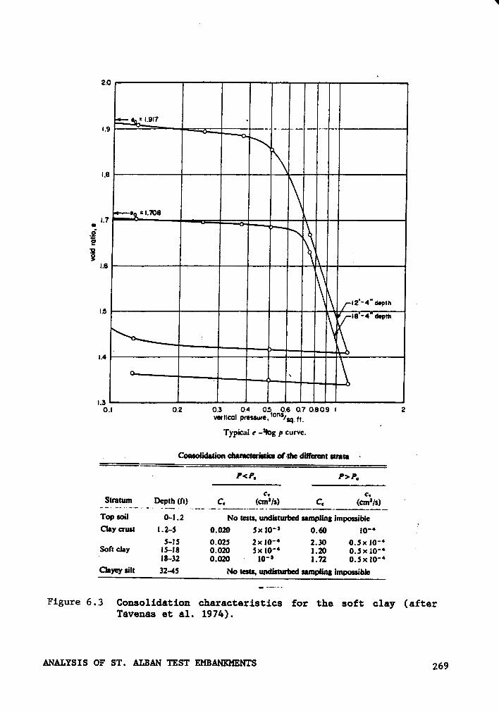
W
2.0I —
Ü“ —$llIl‘I|I—
·
1.7 W L
N .9E Ii—IIIIIIllM
" " ia -4 msnl
l
_
•
E------.!0.l 0.2 0.3 0.4 0.5 0.6 0.7 0.80.9 I 2
vertical pressure,'°“‘/sq_"_
Typical c -’i0g p curve.
. Cousolidatiou eh•mcterist' af-the dllferent strsta ·’
- P<P, P>P,
cw C1_ H vlßftzlh (Tl) C, (¢m‘/s) C, (cm*/s) °
Top soil 0-I .2 No tests, undlsturbed sampllng impossible'Clay crust I.2-5 0.020 5x l0" 0.60 l0"
,7
5-15 0.025 2x l0" 2.30 0.5><10"Soft da! 15-18 0.020 5xl0" 1.20 0.5x10"‘
l8—32 0.020 · l0" 1.72 0.5x l0"Clayey silt 32-45 No tests, undisturbed sampling impossible
Figure 6 .3 Cousolidatiou eharacteristics for the soft clay (afterTavenas et al. 1974).
ANALYSIS OF ST. ALBAN TEST EMBANKMENTS 269
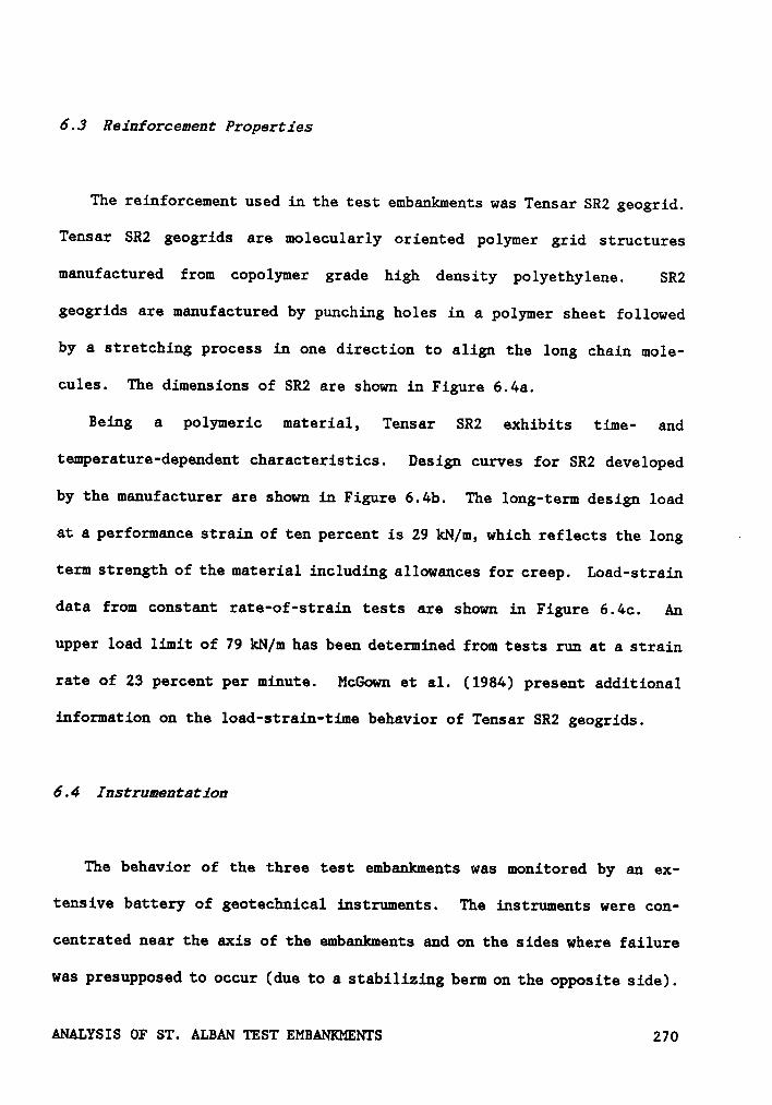
6.3 Reinforcement Properties
The reinforcement used in the test embankments was Tensar SR2 geogrid.
Tensar SR2 geogrids are molecularly oriented polymer grid structures
manufactured from copolymer grade high density polyethylene. SR2
geogrids are manufactured by punching holes in a polymer sheet followed
by a stretching process in one direction to align the long chain mole-
cules. The dimensions of SR2 are shown in Figure 6.4a.
Being a polymeric material, Tensar SR2 exhibits time- and
temperature-dependent characteristics. Design curves for SR2 developed
by the manufacturer are shown in Figure 6.4b. The long-term design load
at a performance strain of ten percent is 29 kN/m, which reflects the long ~
term strength of the material including allowances for creep. Load-strain
data from constant rate-of-strain tests are shown in Figure 6.4c. An
upper load limit of 79 kN/m has been determined from tests run at a strain
rate of 23 percent per minute. McGown et al. (1984) present additional
information on the load-strain-time behavior of Tensar SR2 geogrids.
6.4 Instrumeutation
The behavior of the three test embankments was monitored by an ex-
tensive battery of geotechnical instruments. The instruments were con-
centrated near the axis of the embankments and on the sides where failure
was presupposed to occur (due to a stabilizing berm on the opposite side).
ANALYSIS OF ST. ALBAN TEST EMBANKMENTS 270
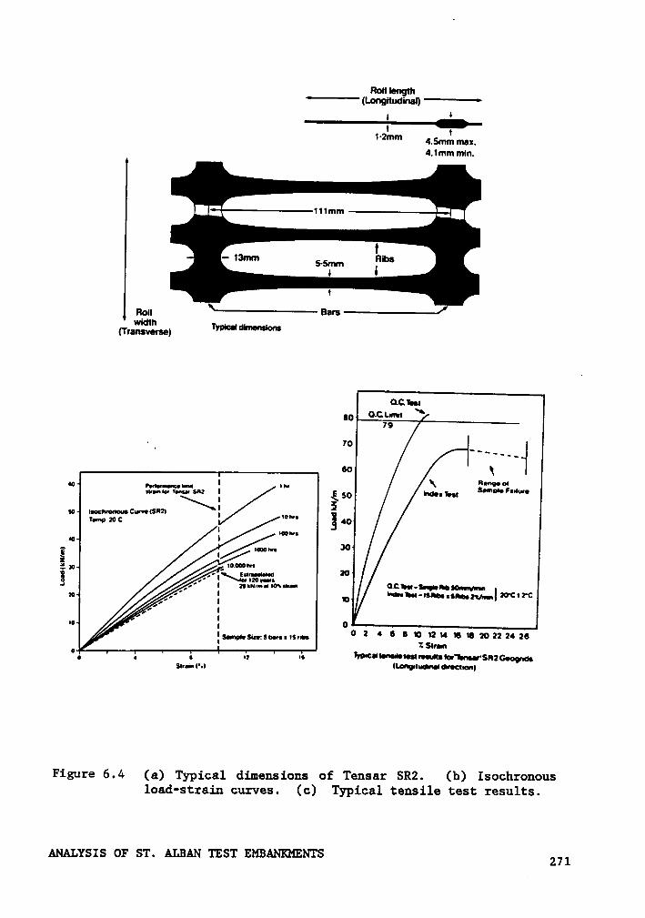
Rolllength°"l(LongItudinaI)*i—•
‘ Ü
' eVzmm 4.5mm max.4.1mm min.
I•- 13mm 5_5mm Ribs6 II
Barsnraxsßvfru)Typiutdlmonsöons
o6<:¥•••,0 0.¢:L•«•«
‘
.~
+‘°
X‘°I ·~ {So
„,}__,„_§:.„"‘:.°I.„....
' z’° '¢.‘I„°".T°„;‘°é"°“"°"”" I ·•~- imI INN;
49 l
E30ä N _ 60.0wm
x ,-·’•\£;'I?6"‘„':‘1 *°4 ’/ Izsnnmmuosuvun;9’,¤”{ n *¢l~•I—|$@•45@')g,„-JKTCITC
. IIl I 0:s•«•p••s6;«;s¤•«„•s„••°
2 ‘° '
2;:** *6**29222* 28UX!
°°
„ . I; I; VYP•¢l!•0I•|•|••1•!I•dl•|¤r"hn••‘$R2G•og•9;
sum t•.6 (Lo••9•Iua•n•I¢r•cI•¤n)
Figure 6.4 (a) Typical dimensions of Tensar SR2. (b) Isochronousload-straiu curves. (c) Typical tensile test results.
ANALYSIS OF ST. ALBAN TEST EMBANKMENTS 271

The layout of instrumentation used for each embankment was similar to
facilitate direct comparisons of behavior.
Pore pressures in the foundation were monitored with electrical, hy-
draulic and pneumatic piezometers; movements of the fill and foundation
soils were monitored using settlement plates, surface displacement monu-
ments, and horizontal and vertical inclinometers. Strains in the foun-
dation soils were measured using electrical and magnetic extensometers.
Measurements of vertical and horizontal stresses in the embankment were
obtained using total pressure cells.
The behavior of the Tensar geogrid was monitored using a specially
designed load cell to measure the tensile load in the geogrid with strains
in the geogrid measured using Bison strain gages.
Movement between the soil and the geogrid was monitored by differen-
tial extensometers. No movement between the soil and the geogrid was
recorded in the strip reinforced embankment, and these types of measure-
ments were not made in the geocell mattress embankment.
The data provided by these instruments provides a good basis for
comparing the results of analytical studies to the measured performance
of the embankments. Further details of the instrumentation can be found
in Busbridge et al. (1985).
6.5 Field Test Results
Construction of the three embankments took place during August to
October, 1984. The strip reinforced embankment was constructed first,
ANALYSIS OF ST. ALBAN TEST EMBANKMENTS 272
followed by the control embankment and finally by the geocell mattress
embankment.
Details of the construction procedures employed can be found in
Busbridge et al. (1985). Each embankment was constructed in the same
general manner. An initial working pad was constructed over a large plan
area (30m x 70m) to a height of 1.5m, over a three- to four-day period.
Following this, two lifts of 0.3m thickness were added each day on a
smaller plan area until failure occurred. This sequence of fill placement
provided stabilizing berms 1.5 m high on three sides of the embankment
to induce failure in a preferred direction.
The failure of the strip reinforced embankment and the control
embankment were sudden, occurring in 30 to 60 seconds with no prior sign
of distress. The failure of the geocell mattress embankment occurred
during the evening or night when the site was unattended. All three
embankments failed in a rotational slip mode with the fill and foundation
soil moving as a solid block. In general, the crest of the embankment
moved down about 1.5 to 2.0 meters, with the toe of the embankment heaving
a similar amount.
Table 6.1 summarizes the height of the fill at failure and the depth
of the failure surface for the three embankments and also for an
embankment constructed to failure at this site in 1972 as reported by La
Rochelle et al. (1974). Also shown are the unit weights and the friction
angle of the fill for each of the embankments.
ANALYSIS OF ST. ALBAN TEST EMBANKMENTS 273

Table 6.1 Height to failure of test embankments.
Height at Depth of Fill ParametersEmbankment Failure, m Failure Surface, m Y, kN/m3 ¢
1972 Unreinforced 4.0 4.0 18.9 44
1984 Control 5.1 4.0-5.5 18.1 34
1984 Strip Reinforced 6.0 4.0-5.5 16.9 34
1984 Geocell Mattress 4.5 3.0-6.0 18.2 34
ANALYSIS OF ST. ALBAN TEST EMBANKMENTS 274
The behavior of the three embankments was very similar in terms of
pore pressure response in the foundation, settlement, and horizontal
movements.
The pore pressure response can be described in terms of the pore
pressure parameter §'=-iää-= change in pore pressure/change in total
vertical stress. The E value in the soft clay was around 0.5 until the
embankment heights reached about 2.8m. A rise of the incremental value
of E to about 1.0 then occurred, and at a height of 4.5 to 5.0m, the E
value became greater than 1.0 and approached 1.3. In a study of the 1972
embankment failure, Tavenas and Leroueil (1980) concluded that initial
low values of B E were due to the effects of preconsolidation and re-
sultant high values of the coefficient of consolidation. The onset of
E = 1.0 was interpreted as the point at which the vertical effective
stress 6} exceeded the preconsolidation pressure 6} and the coefficient
of consolidation is reduced by a factor of 10 to 50 to approach an un-
drained condition. The increase in the value of E above one was inter-
preted as the onset of local failure in the soft clay soils.
The settlement behavior of the three embankments was nearly identical.
During the first four days of construction, settlement under the
centerline was between four and seven millimeters per day. On the fifth
day, this rate increased to approximately 25 mm/day under the strip re-
inforced and the geocell mattress embankments and to 35 mm/day under the
control embankment. The rate increased to 35 mm/day under the strip re-
inforced embankment from the sixth day until failure. The total settle-
ments under the centerline, just prior to failure, were 240 mm, 223 mm
ANALYSIS OF ST. ALBAN TEST EMBANKMENTS 275
and 230 mm for the control, the strip reinforced and the geocell mattress
embankments, respectively.
The horizontal movements measured at the toe of the fill were similar
for each embankment. In general, small movements were recorded below
depths of 6.5 meters. Between depths of 1.5 to 6.5 m (the soft clay zone),
lateral movements on the order of 50 to 100+ m were measured prior to
failure. Movements decreased significantly with distance from the toe,
averaging 60 and 20 percent of the toe movements at distances of three
and eight meters from the toe.
6.6 Limit Equilibrium Analyses
6.6.1 Analyses by La Rochelle et al. and Busbridge et al.
La Rochelle et al. (1974) performed comprehensive analyses of the 1972
test embankment to develop a better understanding of the relationship
between shear strength parameters derived from field and laboratory tests
and the factors of safety obtained from slope stability analyses. These
studies included several different assumptions concerning strength mobi-
lized in the fill, strengths to use for the weathered crust, and strengths
(laboratory or field) to use for the soft clay below the crust. Figure
6.5 shows the strength hypotheses considered in the crust and soft soils.
From this work, La Rochelle et al. showed that reasonable factors of
safety from stability analyses were obtained using residual strength
values for the crust soil and the foundation soils. The residual strength
ANALYSIS OF ST. ALBAN TEST EMBANKMENTS 276

cu I WH:
OO 200 400 600 800 I000 I 200 IÄOO 1600|utI strengen I
I® I/ I I—— med-depth strenqtn
J- - - -2r.' : •"'° ;•-‘--_--0|I\¢V¢l|·/Z
lwenqzn [PQ;I{
I . . . . . 1 . ._·1, I
II
I I
strength (ITtest•I1I I I 1
1 II
II
13 -- s .-- -...1..- . .1-- . 1I1 1@7 1 1 I 1 I
I 1 1 1 ‘II2 —-
IJ - -- I-..--...1.I -- ..I1
I I I I 1I 1 1 1 I I I1 - . 1 1.-.n
III I1 E 1 I 1 1I6 ~—~—~· ·\‘ --—I -'-—- 1---- - -- ’
1II
I rcstducl vohes-
I
18 --,1 ¤ UU tests dem•0 5 03 I '
I ‘I I I
1.· uu testx can
-020‘ I I
Figure 6 ·5 Undrained shear strength profiles of St. Alban site de-termined by different hypotheses (La Rochelle et al . _1974).
ANALYSIS OF ST. ALBAN TEST EMBANKMENTS 277
was defined as the undrained shear strength from CIU or UU laboratory
tests at a strain of 15 percent. This concept later became known as Un-
drained Strength At Large Strains (USALS) (Trak et al. 1980). It is in-
teresting to note that for material below the crust, the USALS profile
corresponds closely to 0.9 times the average vane shear strength profile.
The design and back analyses performed by Busbridge et al. (1985) were
based on the USALS strength profile shown in Figure 6.5. These analyses
were undertaken using three slope stability computer programs. All three
are based on limiting equilibrium of a circular failure surface. Two
programs were for the analysis of embankments without reinforcement, one
based on Bishop°s Modified Method (Bishop, 1955) and the other based on
the method proposed by Sarma (1973). The third program was based on a
circular failure surface through the foundation with determination of
moment equilibrium based upon the weight applied by the fill. This pro-
gram incorporated a stabilizing moment due to a single horizontal rein-
forcing force at the base of the embankment. This program was calibrated
for unreinforced cases by comparing factor of safety results with results
from the other two programs. A description of this program was given by
Milligan and La Rochelle (1984).
Preconstruction stability analyses were based on the USALS shear
strength profile shown in Figure 6.5, residual strength profile 1 in the
crust and fill parameters of the 1972 embankment shown in Table 6.1. With
these properties, a height to failure of 4.0 m was calculated for the
control embankment, which was the failure height of the 1972 test
embankment. A height to failure of 5.2 m was calculated for the strip
ANALYSIS OF ST. ALBAN TEST EMBANKMENTS 278
reinforced embankment based on a reinforcement strength of 158 kN/m (two
times the quality control strength to account for two layers of SR2).
The quality control strength was used because rapid failure was expected.
Following the field trials an investigation of the foundation shear
strength revealed that although the average vane shear strengths in the
soft clay beneath the crust were nearly identical for the three test
embankments, there were large differences in the vane shear strengths in
the crust. Based on this finding, Busbridge et al. reanalyzed the unre-
inforced embankments using the various assumptions for crust strength
shown in Figure 6.5. From these analyses, they concluded that the mid-
depth assumption shown in Figure 6.5 was the most appropriate. Thus, the
strip reinforced and geocell mattress embankment locations were analyzed
using the measured vane shear strength profile (corrected to agree with
USALS by applying a 0.9 correction factor) with the mid-depth assumption
for the crust to obtain calculated, unreinforced heights at these lo-
cations of 4.6m and 4.0m. Further, they determined that reinforcing
forces of 123 kN/m and 64 kN/m would be required to obtain the observed
failure heights of 6.2 and 4.7 m. (These fill heights include an allow-
ance for settlements which occurred during construction.) Thus Busbridge
et al. (1985) attributed the difference in behavior of the test fills to
differences in the strength of the crust at the three locations.
ANALYSIS OF ST. ALBAN TEST EMBANKMENTS 279
6.6.2 Analyses with STABGM
Analyses of the strip reinforced embankment were made during the
course of this study using STABGM (Duncan et al. 1985), a slope stability
program for analysis of reinforced embankments based on Bishop's Modified
Method. This program is somewhat more general than the one used by
Busbridge et al. in that horizontal layers of reinforcement may be placed
at any height in the embankment, more than one layer of reinforcement may
be specified, and either horizontal or tangential orientation of the re-
inforcement may be considered.
A limited parametric study using STABGM was made. The crust strength
used was the mid-depth strength values reported by Busbridge et al. (1985)
for the area where the strip reinforced embankment was located. The av-
erage vane shear strength profiles measured during the post failure in-
vestigation were about 10 to 20 percent greater than the average vane
shear strength profile reported for the 1972 investigation (which are
shown in Figures 6.1 and 6.5). Applying the 0.9 factor to convert average
vane shear strengths to USALS strengths, results in a strength profile
about the same as the 1972 average vane shear strength profile. Hence,
the average vane shear strength profile from Figure 6.5 was used below
the crust.
For an embankment height of 6.0 m, the factors of safety shown in
Figure 6.6 were obtained for various reinforcement strengths. The factor
of safety was determined for both tangential and horizontal orientation
of the reinforcement at failure. It may be seen that the factor of safety
ANALYSIS OF ST. ALBAN TEST EMBANKMENTS 280
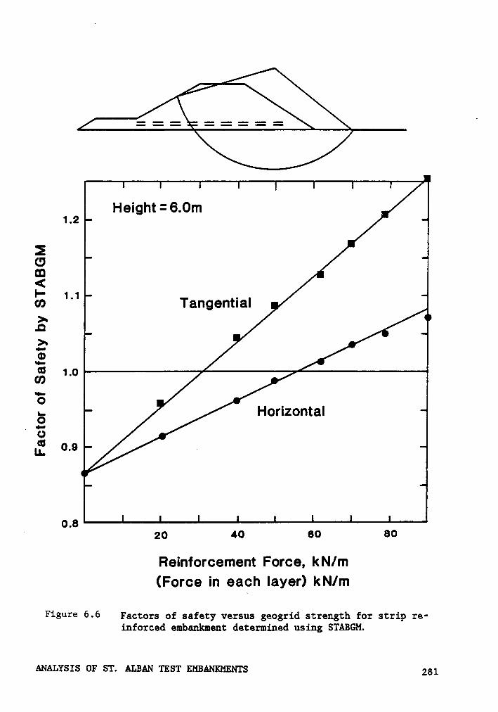
ÄHelght = 6.0m 21.2
ECJE
E 1.1 .rn Tangentnal>~>1tl0:
“ .{E 1 0•W-o&0
. Ol!
SLL 0.6
0.8‘ 20 40 60 80
Relnforcement Force, kN/m(Force in each layer) kN/m
Figure 6-6 Factors of safety versus geogrid strength for strip re-inforced embankment determined using STABGM.
Ammsxs or sr. mm rrsw zmmmms 281
assuming a tangential orientation is always greater the factor of safety
assuming a horizontal orientation. At a factor of safety equal to unity,
which is taken as the point of limiting equilibrium, the analyses show
that mobilized reinforcement forces of about 56 and 30 kN/m/layer would
required to maintain stability for the horizontal and tangential orien-
tations, respectively.
A calculated failure height of 4.9 m for an unreinforced embankment
based on the strength profile under the strip reinforced embankment was
obtained using STABGM. This compares to the value of 4.6 m determined
by Busbridge et al. (1985). Thus, the results obtained using STABGM are
slightly less conservative than those obtained by Busbridge et al. (1985)y
for the same soil strengths.
6.7 Finite Element Analyses
6.7.1 General
The behavior of the test embankments was also analyzed using finite
element techniques. Three types of finite element programs were used for
the analyses conducted in this study. The strip reinforced embankment
was analyzed using CON2D86, which was described in Chapter III, and
SSTIPN, a soi1·structure interaction program based upon the Duncan-Chang
hyperbolic model (Duncan and Chang, 1970). The geocell mattress
embankment was analyzed using SSTIPG, a program developed by Low and
Duncan (1985), in which a special mattress element was incorporated for
ANALYSIS OF ST. ALBAN TEST EMBANKMENTS 282
particular application to Tensar geocells. Analyses of the strip rein-
forced and geocell mattress embankments with no reinforcement were made
for comparison purposes.
The analyses simulated as closely as possible the actual construction
sequence and rate. The template used in the analyses is shown in Figure
6.7 and was modified as needed to fit the various analyses. In the ana-
lyses using CON2D86, the foundation soils were represented by eight node
elements in four layers. One layer each was used for the clay crust and
for the clayey silt and two layers were used to represent the soft clay
layer located 1.5 m to 6.5 m below the surface. In the CON2D86 analyses,
eight construction layers were used, with the reinforcement placed in two
layers. The first two construction layers raised the embankment height
to 1.5 m, and were placed over a period of three days. The third layer
was 0.5 m thick, and was placed in one day. The remaining layers were
0.8 m thick, and were placed in time increments of 1.2 days to correspond
to the loading rate as constructed.
In the analyses using SSTIPN, the eight-node elements from the CON2D86
mesh were subdivided into four-node elements, and the same geometry was
um.Nmemmumümlwuswmuudmtmuamhws Mama
constraint in SSTIPN, the reinforcement was placed after the second con-
struction layer, but still in two layers at the proper height. SSTIPN
does not model consolidation behavior or time effects and thus the ana-
lyses assumed undrained conditions in the foundation. Above the re-
inforcement layers, the same loading increments were used as in the
CON2D86 analyses.
ANALYSIS OF ST. ALBAN TEST EMBANKMENTS 283
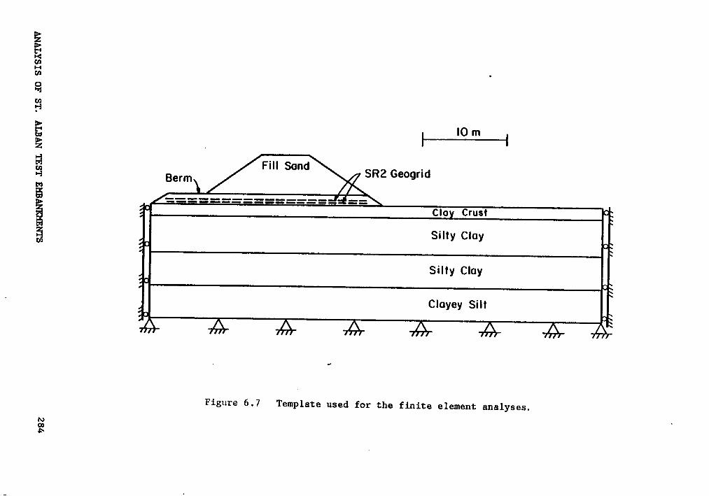
•i••§
•<4
ui3}EQ
{S..
aaE.2
EE
4S
EG
aaO
J„-¤
gg4.:
(Ü
o
xl
<··~
N·¤ev
¤g33
‘¤«E
‘2N.6ca*5
<.
BP~
Cu
EL.
evCD
ANALYSIS
OF
ST.ALBAN
TESTEM
BANKMENTS
284
·I
In the analysis of the geocell mattress embankment, the geometry used
was identical to that used in the SSTIPN analyses except that the first
construction layer was one meter high to accommodate placement of the
geocell mattress.
In the CONZD86 and SSTIPN analyses the reinforcement was modelled as
a standard bar element. A stiffness of 1390 kN/m-width was used for the
geogrid. This value was determined from the quality control tensile test
curve for a strain of two percent, roughly the strain at failure of the
soft, sensitive foundation soils.
6.7.2 Soil Parameters
6.7.2.1 Cam Clay Model
The soil parameters used in the analyses using CON2D86 are shown in
Table 6.2. The foundation soil profile was divided into three zones re-
presenting the clay crust, the soft silty clay and the soft clayey silt.
The parameters were determined in a straightforward manner using the data
shown in Figures 6.1 to 6.3. Permeability values used were obtained from
Tavenas et al. (1983) based on a laboratory and field study of the St.
Alban site.
Effective stress parameters ¢’and c' are shown in Figure 6.1 for the
soil at a depth of five to ten meters. These parameters correspond to M
= 1.11 and py = 3.75 kPa. For the soft clay zone from 1.5 to 5 m a value
ANALYSIS OF ST. ALBAN TEST EMBANKMENTS 285
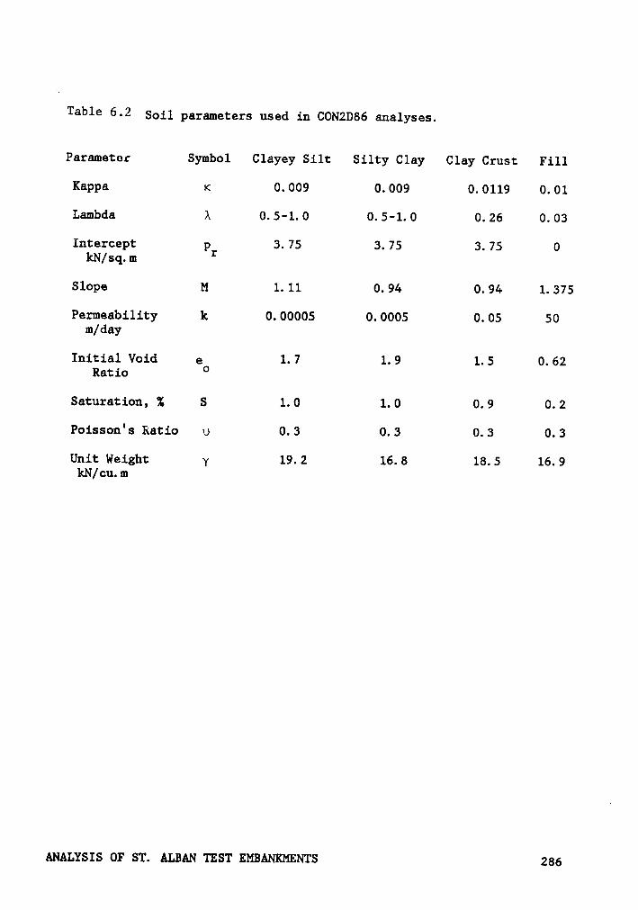
Table 6·2 Soil parameters used in CON2D86 analyses.
Parameter Symbol Clayey Silt Silty Clay Clay Crust Fill
Kappa K 0.009 0.009 0.0119 0.01
Lambda A 0.5-1.0 0.5-1.0 0.26 0.03
Intercept p 3.75 3.75 3.75 0kN/sq.m Y
Slope M 1.11 0.94 0.94 1.375
Permeability k 0.00005 0.0005 0.05 50m/day
Initial Void e 1.7 1.9 1.5 0.62Ratio °
Saturation, % S 1.0 1.0 0.9 0.2
Poisson's Ratio 0 0.3 0.3 0.3 0.3
Unit Weight Y 19.2 16.8 18.5 16.9kN/cu.m
ANALYSIS OF ST. ALBAN TEST EMBANKMENTS 286
of M = 0.94 was used based on the relationship between M and undrained
shear strength described in Section 3.2.3.
For the Cam Clay model employed in CON2D86, the parameter Pb deter-
mines whether the soil is undergoing elastic or plastic behavior. Because
sensitive clays develop large strains when loaded past Pb, the determi-
nation of 1*0 for these analyses is particularly important. Two ap-
proaches to the determination of Pb were used. First, the value of Pb
was determined based on the 1QgV and Pcyi values reported by Tavenas et
al. (1974) (the Pcwraté shown in Figure 6.1) where Pcyy averages 0.7 times
Pcpn A second approach was to determine Pb for a stress level of 0.6,
the point where Tavenas et al. (1974) indicated that elastic behavior
ceases in the stress-strain curve shown in Figure 6.2. The consequences
of these different assumptions are discussed in the section describing
the finite element results.
6.7.2.2 Hyperbolic Node]
The soil parameters used in the programs SSTIPN and SSTIPG are shown
in Table 6.3. These analyses were performed for the undrained case and
hence undrained shear strength parameters were used for the foundation
soils. The average vane shear strength profile shown in Figure 6.1 was
used for the foundation soils. For the crust soils the mid-depth strength
values reported by Busbridge et al. (1985) were used, in accordance with
the discussion in section 6.6.1.
ANALYSIS OF ST. ALBAN TEST EMBANKMENTS 287
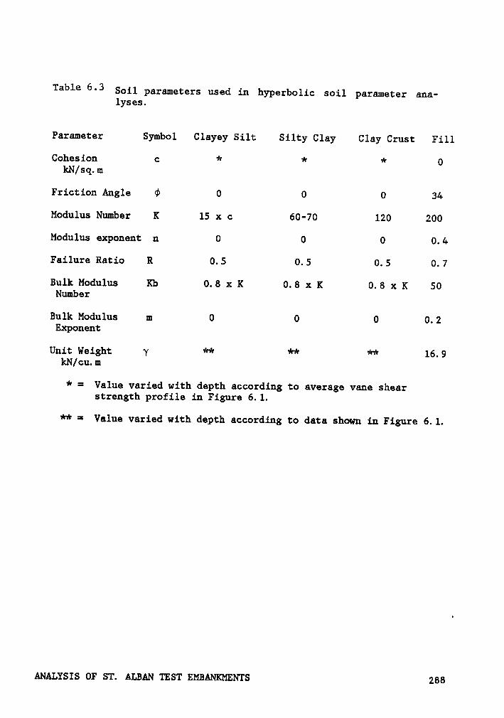
Table 6·3 Soil parameters used in. hyperbolic soil parameter ana-lyses.
Parameter Symbol Clayey Silt Silty Clay Clay Crust Fill
Cohesion c * * * 0kN/sq.m
Friction Angle ¢ O 0 0 34
Modulus Number K 15 x c 60-70 120 200
Modulus exponent u 0 0 0 0.4
Failure Ratio R 0.5 0.5 0.5 0.7
Bulk Modulus Kb 0.8 x K 0.8 x K 0.8 x K S0Number
Bulk Modulus m 0 0 0 0.2Exponent
Unit Weight Y ** ** ** 16.9kN/cu.m
* = Value varied with depth according to average vane shearstrength profile in Figure 6.1.
** = Value varied with depth according to data shown in Figure 6.1.
ANALYSIS OF ST. ALBAN TEST EMBANKMENTS 288
The modulus number for the foundation soils was determined from data
presented by Tavenas et al. (1974). These authors presented values of
Eh determined from unconfined, UU and CIU compression tests as a function
of depth. The Eh values were defined as the secant moduli at a stress
level of 50 percent. For the determination of K, the modulus number, it
is necessary to determine values of Eh the initial tangent modulus. E}
values were calculated from the Eh values by taking the Eh values times
a factor of 1.4. The basis for this factor of 1.4 is as follows:
For o = 0 conditions, the tangent modulus can be written (Duncan et
al. 1980) as
Et = E,{1 —[6.1]
Also, 2c = (ol — 63V and thus, = = S, a strength ratio.<“1 — ¤3VEquation 6.1 can be written as
E} = E}1 — Sßßz[62]
If the tangent modulus at a stress level of 25 percent is assumed to be
parallel to the Eh modulus, the ratio of-éä or-éä-can be determined fromEquation 6.2 for known values of gf The failure ratio, äh was determinedby matching hyperbolic stress-strain curves to those from
unconsolidated—undrained tests reported by La Rochelle et al (1974).
Based on these data, it was determined that a representative factor for
initial tangent moduli based on Eh values from UU tests was 1.4. The
values of E} so calculated were used to determine the modulus number K
ANALYSIS OF ST. ALBAN TEST EMBANKMENTS 289
assuming a modulus exponent of zero. Average K values were selected for
each soil layer in the analyses.
In cases where insufficient data was available to define model pa-
rameters, the guidelines provided by Duncan et al. (1980) were used to
estimate parameter values. The bulk modulus values were chosen to provide
a Poisson°s ratio value of 0.3 in the foundation soils. Work by Tavenas
et al. (1974) on the settlement of embankments at the St. Alban site
showed that a value of 0.3 provided much better agreement between calcu-
lated and observed settlement than the typical undrained value of 0.49.
6.7.3 Strip Rainforced Ehbankmant
The results of three finite element analyses using CON2D86 are com-
pared to the measured values of settlement, horizontal movement, re-
inforcement force and piezometric level in Figures 6.8 through 6.11. One
analysis, labelled A in the figures, used the soil strength profile based
on the average vane shear strength profile shown in Figure 6.1, and P}
values based on preconsolidation pressures PCH and PCV reported by
Tavenas et al. (1974). A second analysis (labelled B) was based on the
same shear strength profile, but used P} values determined to provide
plastic behavior in the elements when the stress level reach 0.6. A third
analysis (labelled C), which was performed to represent the unreinforced
condition, had the same soil properties as the second analysis.
The data in Figure 6.8 show that analysis A predicted less settlement
than was measured. The shape of the settlement curve parallels the
ANALYSIS OF ST. ALBAN TEST EMBANKMENTS 290
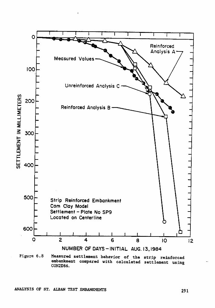
OJ'A
_»· Rennforced
·· A Analysis AMeasured Values „
Aloo °\. . · AUnreinforced Analysis C L p
—\
tn•
*{5 zoo a'I,] Reinforced Analysis B *
I.1:1EE sool-ZLl.1ELU.1I-li(0 4OO
500 Strip Reinforced EmbankmentCam Clay ModelSettlement- Plate No SP9Located on Centerline •
600 .I
IO 2 4 6 8 IO I2
NUMBER OF DAYS··INITIAL AUG. |3,I984. Figure 6.8 Measured settlement behavior of the strip reinforced
embankment compared with calculated settlement using "CON2D86.
ANALYSIS OF ST. ALBAN TEST EMBANKMENTS 291
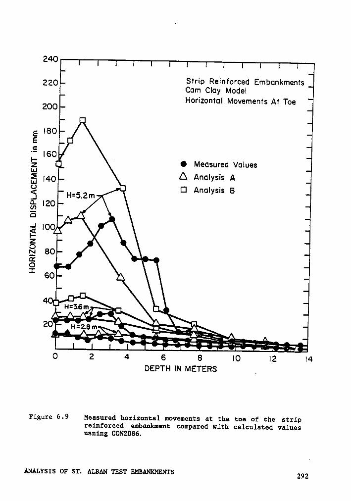
240
220 Strip Reinforced EmbonkmentsCom Cloy ModelHorizontol Movements At Toe200
I
E IC
Q" I O Meosured VoluesnuA Anolysis AEI Anolysis B
IfQ l20E · ^IOOAä¤:E 60 A
.,- II
2°Z
0 2 4 6 8 I0 I2 I4DEPTH IN METERS _
Figure 6•9 Measured horizontal movemeuts at the toe of the stripreinforced embankmeut compared with calculated valuesusuing CON2D86.
Ammsxs OF sr. ALBAN mm- zuammmms 222
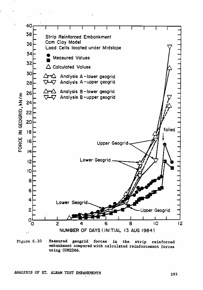
i 40 _'
38 Strip Reinforced Embankment36 Cam Clay Model
Load Cells located under Midslope V
I Measured Values32
A Calculated Values A30 A··A Analysis A—lower geogridgg VW Analysis A-upper geogrid
E 26 A·A Analysis B-lower geogrid\ V-W Analysis B—uppergeogridE24 I?6EE 22 08 2OE I8 Ä} failed
I6 . V .ä Upper Geogrld
{,
0¤— I4I2 Lower Geogrid A v r _.—
-IO{6
4{ 4 I {
4 · I { ILower Geogrid 9//,\
2 9 b Y :0: Upper GeogridO A«;.L.-.
O 2 ‘ 4 6 8 IO I2__ NUMBER OF DAYS IINITIAL I3 AUG |984)
Figure 6.10 Measured geogrid forces in the strip reinforcedembankment compared with calculated reinforcement forcesusing CON2D86.
ANALYSIS or sr. mm msr EMBANKMENTS 293
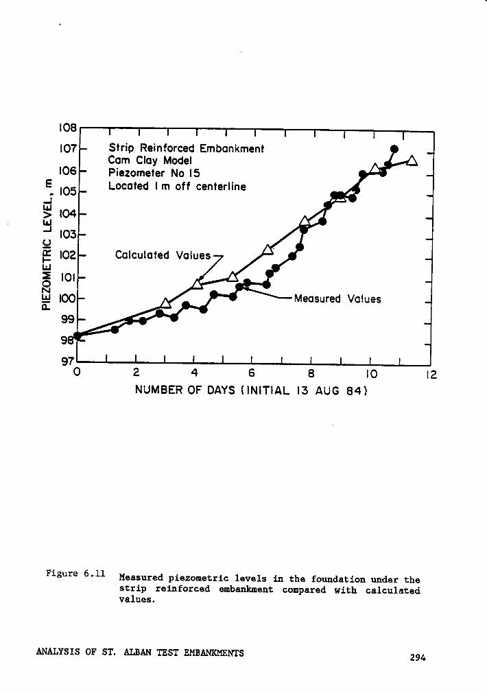
lO8IO? Strip Reinforced EmbankmentCam Clay Model ‘ AIO6 Piezometer No I5 ‘
Located lm aff centerlineM pn,
LnlI Z '°" 4/3 lO3Fj IO2 Calculated Values AN .
g IOI ‘ 4.Q
lgg A Measured Values99 Ä,.9
9?O 2 4 6 8 IO I2
NUMBER OF DAYS llNlTlAL I3 AUG 84)
Figure 6*11 Measured piezometric levels in the foundatiou under thestrip reinforced embaukmeut compared with calculatedvalues.
ANALYSIS 01* ST. ALBAN TEST EMBANKMENTS 294
measured data but the downward break occurred at a much higher applied
pressure in the analysis. This is believed to be attributable to using
too high of values of P} in the analysis. An inspection of element be-
havior in analysis A showed foundation elements to remain in elastic be-
havior up to stress levels of 0.85. Considering the stress-strain data
in Figure 6.3, where plastic behavior begins at a stress level of about
0.6, it was felt that the foundation elements should begin plastic be-
havior at a comparable stress level in the analysis. This was accom-
plished by reducing P} to cause plastic behavior to begin at a stress
level of about 0.6. The consequence of this reduction is apparent in the
results for analysis B shown in Figure 6.8.
It may' be seen that reducing .P} resulted in considerably* more
settlement in the analysis, and better agreement with the measured values.
Indeed, with the reduced P} in analysis B, failure of the reinforced
embankment occurred at a height of 6.0 m, matching the field behavior.
The settlement behavior for analysis C, representing the unreinforced
condition, shows large settlements at an embankment height of 5.2 m, which
may be interpreted as failure of the embankment. While soil conditions
at the control embankment location were slightly different than those at
the strip reinforced embankment location, this unreinforced analysis
matches well with the observed behavior of the control embankment.
Calculated and measured horizontal deformations are compared in Figure
6.9. In the early stages of construction, the calculated and measured
values agree quite well. In analysis A, the absolute magnitude of move-
ment was predicted well, but the precise locations and shape of the
ANALYSIS OF ST. ALBAN TEST EMBANKMENTS 295

movement profiles differ somewhat from the measured values. In analysis
B, the horizontal movements are somewhat larger than those measured. The
horizontal movements occurring in the unreinforced analysis were on the
order of one meter (five to six times larger than those calculated in
analysis B), when the embankment was one meter lower, and are, therefore,
too large to be shown in Figure 6.9.
The reinforcement loads measured in two load cells located under the
midslope of the embankment are shown in Figure 6.10. The measured forces,
which are relatively small, increase as the embankment height increases.
At failure, forces of 15.4 and 11.8 kN/m were measured in the lower and
upper layers, respectively. It seems likely that the location of the load
cells was not appropriate for detecting the maximum force in the re-
inforcement. The failure surface formed near the axis of the embankment,
and the location of greatest stress in the reinforcement would have been
close to the centerline. The calculated forces shown in Figure 6.10
correspond to the location of the load cells in the embankment. The
calculated forces agree relatively well with measured values in the early
stages of construction. When the embankment height increased above four
meters, the calculated forces increased significantly, reaching values
of about 25 kN/m for analysis A and of about 35 kN/m for analysis B at
an embankment height of 6.0 m. In the analyses, the highest reinforcement
forces, under the centerline, were about 29 kN/m/layer for analysis A and
about 69 kN/m/layer for analysis B. The value of force in analysis B is
very close to the strength which could be mobilized in a rapidly loaded
sample of Tensar SR2, as may be deduced from Figure 6.4. It seems likely
ANALYSIS OF ST. ALBAN TEST EMBANKMENTS 296
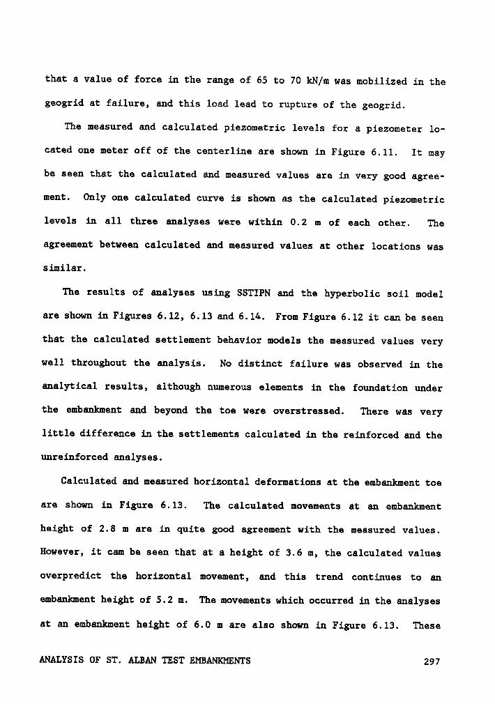
that a value of force in the range of 65 to 70 kN/m was mobilized in the
geogrid at failure, and this load lead to rupture of the geogrid.
The measured and calculated piezometric levels for a piezometer lo-
cated one meter off of the centerline are shown in Figure 6.11. It may
be seen that the calculated and measured values are in very good agree-
ment. Only one calculated curve is shown as the calculated piezometric
levels in all three analyses were within 0.2 m of each other. The
agreement between calculated and measured values at other locations was
similar.
The results of analyses using SSTIPN and the hyperbolic soil model
are shown in Figures 6.12, 6.13 and 6.14. From Figure 6.12 it can be seen
that the calculated settlement behavior models the measured values very
well throughout the analysis. No distinct failure was observed in the
analytical results, although numerous elements in the foundation under
the embankment and beyond the toe were overstressed. There was very
little difference in the settlements calculated in the reinforced and the
unreinforced analyses.
Calculated and measured horizontal deformations at the embankment toe
are shown in Figure 6.13. The calculated movements at an embankment
height of 2.8 m are in quite good agreement with the measured values.
However, it cam be seen that at a height of 3.6 m, the calculated values
overpredict the horizontal movement, and this trend continues to an
embankment height of 5.2 m. The movements which occurred in the analyses
at an embankment height of 6.0 m are also shown in Figure 6.13. These
ANALYSIS OF ST. ALBAN TEST EMBANKMENTS 297
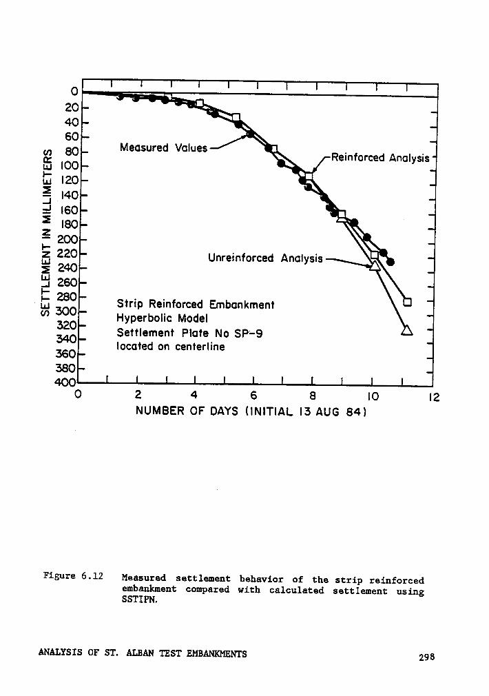
O20240 \‘„GG
M d V I89 eqsureReinforced AnalysisIOOLLJ
l20 ·\§ VI4O ·ri' I6O ‘= _
I8O 2E zoo \ 9E ZZO Unreinforced Anal ' 'Lu ysns A5 240E 260IZ 280 . . •· Lu 300 Strip Remforced Embankment"’
320 Hyperbolic Model340 Settlement Plate No SP—9
‘
360 located on centerline380400
0 2 4 6 8 IO I2NUMBER OF DAYS IINITIAI. I3 AUG 84)
Figure 6-12 Measured settlement behavior of the strip reinforcedembankment compared with calculated settlement usingssT11¤N.
ANA1.Ts1s or sT. ALBAN TEST EMBANKMENTS 296
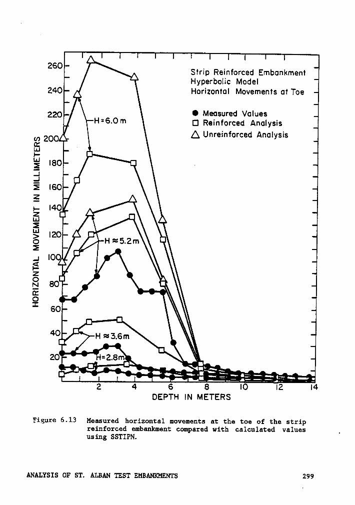
A260Ä Strip Reinforced Embankment
Hyperbolic Model240 ‘ Horizontal Movements at Toe
220 O Measured ValuesI3 Reinforced Analysis
U) ZOO A Unreinforced Analysisa:IB n'§ ISO ¤ -E=l ¤2 ISOE V 4I- |4O AE ' ' ·ui> IZO Ä
· I2_;IO I
fiä Ä
·g 80 ‘
2 SOu
‘I
40 ' \ „uf¤2°M.
°; °°°=€E °' °: "" "°H.l4;4!...;;.Ai„?;Z;‘ ?" Z2 4 S 8 IO I2 I4
DEPTH IN METERS
Figure 6-13 Measured horizontal movements at the toe of the stripreinforced embankment compared with calculated values _using SSTIPN.
ANALYSIS or ST. ALBAN TEST EMBANKMENTS 299
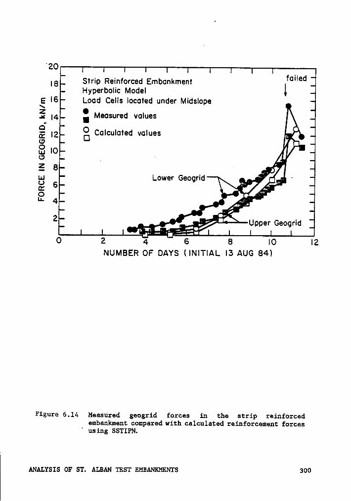
°2O
IB Strip Reinforced Embankment fmledHyperbolic Model I
E I6 Load Cells located under Midslope\
E I4
=
Measuredvalues2
I2 Calculated values _,·o I n3 IO I
ca „ · rlE8u.:Lower Geogrid „ _ ¤_„~ ‘62lv
J
2 , n} ·E M r ‘_=•.) Upper GeogndI.; —• •.·__·‘_':,_-
O 2 4 6 8 IO I2NUMBER OF DAYS (INITIAL I3 AUG 84I
Figure 6.14 Measured geogrid forces in the strip reinforcedembankment compared with calculeted reinforcement forces
' using SSTIPN.
ANALYSIS OF ST. ALBAN TEST EMBANKMENTS soo
movements are quite large, but do not yet represent failed conditions,
although the incremental movements are significant.
Finally, the calculated values of geogrid force are compared to the
measured values in Figure 6.14. The calculated values underpredict the
measured geogrid forces slightly through the entire analysis. It should
be noted that geogrid forces do not occur in the analysis until the third
load step due to constraints in the program. Thus forces which may have
developed in the early stages of construction were not included in the
calculated values. The calculated forces in the geogrid under the
centerline were 20 and 16 kN/m for the lower and upper layers, about four
to eight kN/m greater than the calculated values under the midslope.
6.7.4 6606611 Hattress Ehbankment
The soil parameters used for the analyses of the geocell mattress
using SSTIPG were identical to those used in the SSTIPN analyses of the
strip reinforced embankment except for the strength of the clay crust
layer. The strength of the clay crust was taken as the mid-depth vane
shear strength values reported by Busbridge et al. (1985). These
strengths were about 75 percent of the strength of the clay crust at the
strip reinforced embankment location.
The results of reinforced and unreinforced analyses of the geocell
embankment are shown in Figures 6.15, 6.16 and 6.17. The calculated
settlement behavior agrees with the measured values very well. As in the
hyperbolic model analyses of the strip reinforced embankment, the forces
ANALYSIS OF ST. ALBAN TEST EMBANKMENTS 301
calculated in the geocell mattress did not reach failure values. However,
large incremental settlements did occur in the analyses when the
embankment height was increased to 5.2 m.
The calculated and measured values of horizontal deformation at the
toe are compared in Figure 6.16. The agreement is reasonably good, with
calculated values being somewhat greater than measured values at an
embankment height of 3.6 m. At an embankment height of 4.4, the measured
values of horizontal deformation are slightly larger than those calcu-
lated. These measured values represent conditions just prior to failure.
Failure occurred in the field at an embankment height of 4.6 m. At the
embankment heights shown in Figure 6.16, the reinforced and unreinforced
analyses show minor differences in the horizontal deformation behavior.
When the height in the analyses was increased to 5.2 m, the calculated
difference between the reinforced and the unreinforced embankments became
more pronounced, with movements at the toe of the unreinforced embankment
being about 80 to 100 mm greater than corresponding movements in the re-
inforced embankment. The differences became significantly larger when
the fill height was increased to 6.0 m.
Comparisons of the measured and calculated force in the geogrid are
shown in Figure 6.17. Because a composite element was used to represent
the geocell mattress, the program SSTIPG does not explicitly provide re-
inforcement forces. However, the force can be calculated from the strains
which occur in any mattress element. it can be seen in Figure 6.17 that
the calculated forces are less than those measured. The measured values
have an initial force induced at 1.5 days, which was induced during con-
ANALYSIS OF ST. ALBAN TEST EMBANKMENTS 302
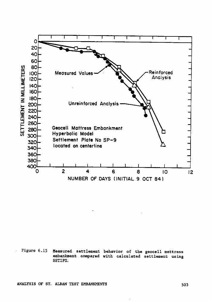
OZC40
IN;
SC80 "Ü 499 Measured Values · \A R°‘"f°"°?d
E IZO · AnalysnsE ·1E l4O .. ^Z IBC , . nE
200 Unrelnforced Anolysns HALu 220
ä 240l- 280 Geocell Mattress Embankment .ä 300 Hyperbolic Model
320 Settlement Plate No SP-9340 located on centerline ^360380400
0 2 4 6 8 l0 I2NUMBER OF DAYS (lNlTlAL 9 OCT 84)
· Figure 6.15 Measured settlement behavior of the geocell mattressembankment compared with calculated Settlement usingSSTIPG.
ANALYSIS or ST. ALBAN TEST EMBANKMENTS 303
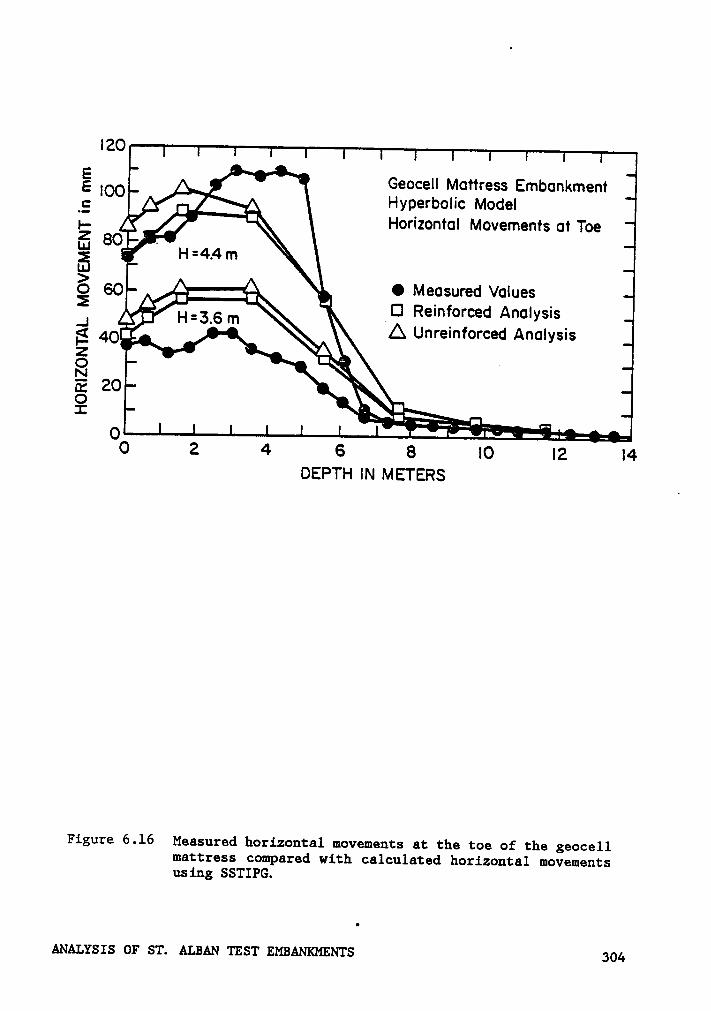
IZO
A1 ‘ Geocell Mattress Embankment
E A Hyperbolic Model,_A I ' Horizontal Movements at Toe
E 80 °’
gg .4 O Measured ValuesE A}? " _CI Reinforced AnalysisE;}
·A Unreinforced AnalysisI- 40 „. AZ A —
==- .S ‘\E 20 E
° \'I ”—* ll ..
O 2 4 6 8 IO I2 I4DEPTH IN METERS
Figure 6-16 Measured horizontal movements at the toe of the geocellmattress compared with calculated horizontal movementsusing SSTIPG.
ANALYSIS OF ST. ALBAN TEST EMBANKMENTS 304
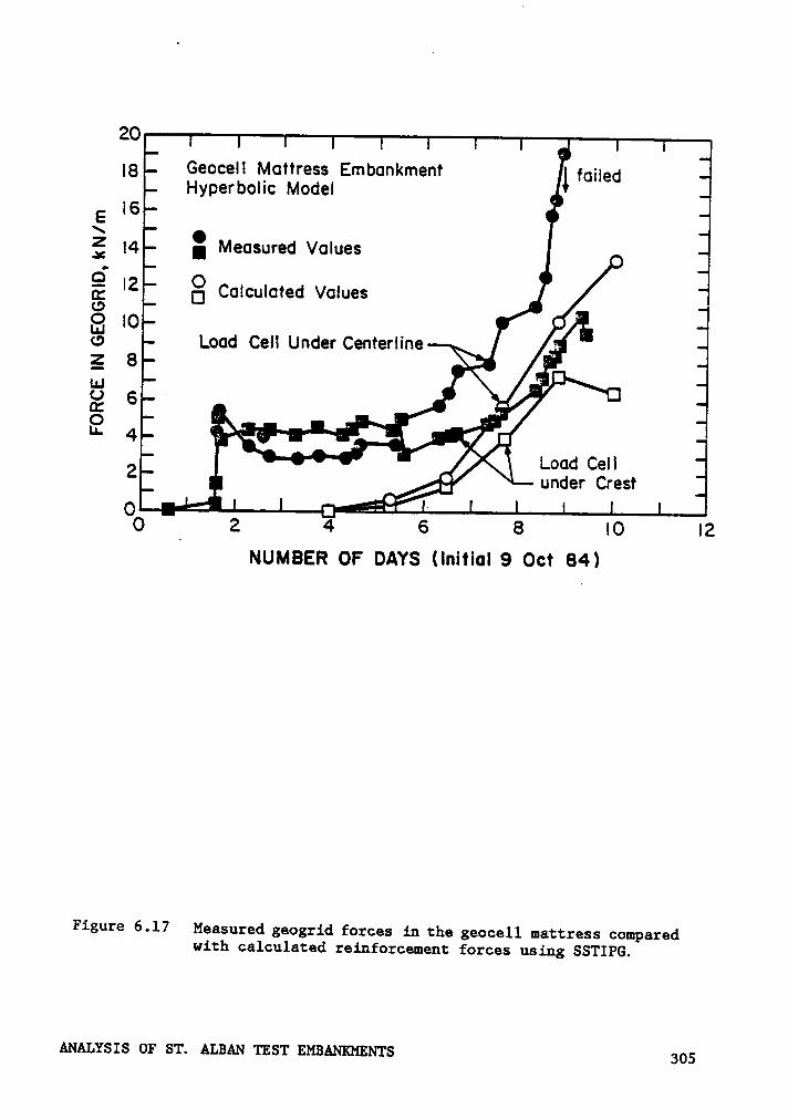
ZOgg Geocell Mntiress Embnnkment lfggggdHyperbolic Model J
E I6E ‘
M 6 v I_! I4 I ensure n ues°
ä (2 Calculnted Values Jä IO•.29 Lond Cell Under Centerline _8 \ >-I.I.I 6 er °L" 4 n’
{ L666 Cell_I
O 2 4 6 8 IO I2NUMBER OF DAYS (Initial 9 Oct 84)
Figure 6.17 Measured geogrid forces in the geocell mattress comparedwith calculated reinforcement forces using SSTIPG.
Ammsxs or sw. ALBAN TEST Eußmomms 305
struction of the mattress, and this force remains relatively constant
until day five (fill height of 2.8 m). If the measured values are shifted
to eliminate this initial prestress, the measured and calculated values
would agree reasonably well. It may be seen that both the measured and
the calculated values show the force at the centerline to be larger than
the force under the crest, as would be expected.
The analyses performed do not shed much light on why the geocell
mattress embankment failed at a height less than the control embankment.
The analyses do show that distress was beginning to occur in the founda-
tion soils at fill heights around 4.5 m. Coupling this with the known
brittle behavior of highly sensitive soils, it is reasonable to conclude
that failure might occur at any height above about 4.5 m.
6.8 Discussion
The results of the analyses performed using CON2D86 indicate that
calculated behavior is very sensitive to the value of mean preconsol-
idation pressure Pb used in the analyses. A somewhat better prediction
of settlement behavior was obtained when the IMO values used in the
analysis were reduced, but this resulted in a less satisfactory prediction
of horizontal movements. The forces in the geogrid predicted in these
analyses matched measured values well at fill heights less than about four
meters. Above this height the analyses showed considerably higher forces
than measured in the field.
ANALYSIS OF ST. ALBAN TEST EMBANKMENTS 306
The results from analyses using the hyperbolic soil model showed re-
markable agreement to the measured settlement data and reasonable agree-
ment with the horizontal deformations. This tends to support the method
used to determine the modulus numbers from undrained secant moduli. The
calculated and measured geogrid forces also matched reasonably well, al-
though the calculated forces were lower than the measured values in the
early stages of the analyses. These results demonstrate that this soil
model can accurately model the behavior of reinforced soil embankments
under working conditions. The determination of a failure height from
hyperbolic model analyses needs to be based on the stress levels in ele-
ments. On this basis, a continuous band of overstressed elements in the
analyses appear to correspond well with the observed field behavior.
The differences obtained between measured and calculated horizontal
movements are in agreement with results reported by Poulos (1972). In
an analysis of a number of case histories, Poulos found that when good
agreement between measured and calculated settlements was obtained, the
predicted horizontal movements were greater than those measured. Among
the reasons cited for the differences were: the difficulty of estimating
Poisson°s ratio of the soil; anisotropy, nonlinear stress-strain behavior
and nonhomogeniety of the soil; and the neglect of certain factors in the
analyses, such as the effect of embankment stiffness and foundation
roughness. When changes in the above factors were made, Poulos found that
the sensitivity of horizontal movement predictions was considerably more
than that of the settlement predictions. The effects of Poisson°s ratio,
ANALYSIS OF ST. ALBAN TEST EMBANKMENTS 307
anisotropy and nonhomogeniety appeared to be the most significant fac-
tors.
All the reinforced analyses showed higher geogrid forces under the
centerline than under the midslope or crest, and it is felt that similar
behavior almost certainly occurred in the field trials. In the CON2D86
analyses, the maximum geogrid load occurred under the centerline and had
values of 24 to 29 kN/m for analysis A and about 70 kN/m for analysis B.
In analysis B the embankment failed when the height was increased to 6.0
m, which matched the field behavior, and these forces are believed to be
representative of the field behavior. The maximum calculated forces in
the strip reinforced analysis from SSTIPN were 20 kN/m in the lower layer
and 16 kN/m in the upper layer, also occurring under the centerline.
These forces are smaller than those determined using CON2D86, as a result
of the smaller deformations calculated in these analyses.
Any interpretation of the force mobilized in the geogrid at failure
must take account of the orientation of the geogrid when failure occurs.
On one hand the orientation at failure can be considered to be horizontal.
For this condition, results of stability analyses indicate that a geogrid
force of 55 to 60 kN/m-width would be mobilized at failure. In the finite
element analyses, the reinforcement force acts in an essentially hori-
zontal direction. The forces calculated at a location consistent with
the observed failure surface were about 65 to 70 kN/m at an embankment
height of 6.0 m. These results appear to be in good agreement with the
stability analyses, and suggest that at failure the mobilized force in
ANALYSIS OF ST. ALBAN TEST EMBANKMNTS 308
the geogrid was near 60 kN/m. This is a reasonable value based on the
load-strain data shown in Figure 6.4.
The calculated behavior of a reinforced embankment is a direct func-
tion of the reinforcement modulus input into the analysis. In this study
only one modulus value was used. This value is believed to provide a
reasonable representation of the field behavior of the geogrid.
6.9 Summary and Conclusions
The goal of the study of the St. Alban embankments was to ascertain
if accurate predictions of reinforced embankment behavior could be made
using straightforward interpretations of soil data. The analyses per-
formed in this study were accomplished with minimal fine-tuning of the
soil parameters. The results of the analyses performed suggest that the
behavior of reinforced embankments on sensitive soils can be modelled
reasonably well using finite element techniques.
ANALYSIS OF ST. ALBAN TEST EMBANKMNTS 309
CHAPTER VII
SUMARY
The studies described herein have been concerned with the development
and application of analytical techniques to reinforced soil foundations
and embankments over weak soils. The primary analytical employed tool
was the finite element method.
During this study an existing finite element computer program was
modified for applications to reinforced soil structures. The computer
program, CON2D86, was developed for the analysis of stresses, displace-
ments, and consolidation of soil masses. The capability of modelling
reinforcement was added through the use of bar elements having axial
stiffness but no flexural stiffness. In addition, the program was re-
written to adopt the efficiencies of structured programming, to eliminate
errors and unused statements, and to provide additional documentation of
the code. An axisymmetric version of the program (CONSAX86) was extended
for analysis of reinforced soil structures through the addition of a
membrane element which has radial stiffness but no flexural stiffness.
A simplified procedure for computing the bearing capacity of rein-
forced sand over soft clay was proposed and compared to laboratory model
tests. Good agreement with available experimental results was obtained,
and based on these comparisons the procedure appears to be suitable for
estimating the ultimate bearing capacity of such systems. Additional
Verification of the proposed method, by comparison with laboratory model
SUMMARY 310

studies and field cases, is desirable. In the meantime, it seems likely
that the judicious use of factors of safety with the proposed method
should result in satisfactory performance of reinforced foundations.
Finite element analyses of model tests of reinforced sand over weak
soils showed good qualitative and fair quantitative agreement with the
measured load-displacement behavior, and they agreed well with the ob-
served modes of failure. The analyses show that the presence of the re-
inforcement reduces the shear stresses in the upper zones of the clay,
resulting in increased load carrying capacity of the reinforced sand-clay
system. Improved understanding of the effect of the compressibility of
the sand and of the initial stresses inherent in compacted sand would
provide greater confidences in the use of the finite element technique
as a design tool. Currently, a design approach combining the finite el-
ement analyses and the proposed bearing capacity analysis technique de-
veloped herein should provide a reasonable engineering solution for
reinforced sand overlying weak soils.
Two well documented and well instrumented reinforced embankments have
analyzed during the course of this investigation. The study of
Mohicanville Dike No. 2 included an evaluation of its performance during
and shortly after construction, and finite element analyses of its be-
havior. The observed performance of the dike showed that it is feasible
to stabilize embankments as high as 25 feet on weak foundations very ef-
fectively using a single layer of reinforcement near the base of the
embankment. Comparison of the calculated and measured reinforcement .
forces indicates that finite element analyses which include the effects
SUMMARY 311
I
of consolidation provide an effective means of estimating the amount of
reinforcing force that would develop during construction, and the rate
at which the force would decrease after construction as the foundation
soils consolidate.
A study of the effects of ageing of the compacted clay fill on the
behavior of Mohicanville Dike No. 2 were inconclusive. While laboratory
studies showed that the compacted fill used at Mohicanville would gain
strength and increase in stiffness with ageing, finite element analyses
showed that increasing the strength and stiffness of the new fill did not
change the computed results significantly. When increased strength and
stiffness were used in the old fill under the reinforcement as well as
the new fill above, the computed and measured behavior were in excellent
agreement. However, it seems likely that some stiffening of the soils,
perhaps the foundation as well as the embankment soils, did occur over
the winter shutdown, probably as a result of consolidation and thixotropy,
and that these changes in properties resulted in the changed behavior that
was clearly evident in the early stages of the second construction season.
The analyses of the St. Alban test embankments were performed to de-
termine if accurate predictions of reinforced embankment behavior could
be made using straightforward interpretations of the soil data. The re-
sults of the analyses, for both the Cam Clay model and the hyperbolic
model, were in good agreement with the field measurements. The measured
geogrid forces, prior to failure of the embankments, were predicted well
by the analyses, showing that working conditions can be modelled well by
finite element analyses. The finite element analyses did not accurately
SUMMARY 312
model the sudden failure of the brittle sensitive clay, but they did show
a large zone of contiguous failed elements at the stage at which failure
occurred.
The successful application of the finite element method to these cases
shows that the method can be used with some confidence for future
projects, as a valid and reliable engineering analysis tool.
7.1 Recommendations for Future Research
7.1.1 Reinforced Foundations.
The use of reinforcement to improve the supporting capacity of layers
of sand over weak clay is still in its infancy. A limited number of model
test studies have shown that reinforcement can increase the capacity of
such systems. However, these model tests have been restricted to rela-
tively small scale, and to a limited number of configurations of re-
inforcement placement, i.e., a single layer at the sand-clay interface.
It appears that further model test studies are warranted, wherein the
location, spacing and type of reinforcing are varied to ascertain the
consequences of such changes. In conducting model tests, the instrumen-
tation of the reinforcement to gather strain or load data would be de-
sirable to obtain information on the mobilized forces in the
reinforcement. This information would aid considerably in fostering im-
proved understanding of the reinforcement-soil interaction mechanism.
SUMMARY 313
4
Additional work is needed to verify the bearing capacity models pro-
posed. As more experimental data, and perhaps field data, become avail-
able, such verification will be possible. The applicability of the
general shear failure mechanism requires that the effect of reinforcement
on the shear strength of a sand be quantified through experimental work.
7.1.2 Reinforced Embaukments
The case history studies have shown that slope stability and finite
element techniques can be used effectively in the design and analysis of
reinforced embankments. However, questions remain about the behavior of
reinforcement in embankments. Conflicting data in the literature con-
cerning pullout resistance indicates that additional work is needed to
clarify the effects of sand density and grain size, and geogrid mesh size
and strength on the soil-reinforcement mechanism. Additional analyses
of case histories are warranted as the data become available to check that
slope stability procedures and the finite element method provide reliable
and consistent results. The development of simplified design procedures
having general applicability is desirable to promote the increased ap-
plication of reinforcing for stabilizing embankments over weak soils.
SUMMARY 314
REFERENCES
Akinmusuru, J. 0. and Akinboldae, J. A. (1981). "Stability of loadedfootings on reinforced soil. Journal of the Geotechnical Engineer-ing Division, American Society of Civil Engineers.l07&colonGT6:819-827.
Andrawes, K. A., McGown, A., Wilson-Fahmy, R. F., and Mashhour, M. M.(1982). "The finite element method of analysis applied to soilgeotextile systems." Proceedings, Second International Conferenceon Geotextiles. Las Vegas, Nevada. August 1-6. 3:695-700.
Atkinson, J. H., and Bransby, P. L. (1978). The Mechanics of Soils -An Introduction ot Critical State Soil Mechanics. McGraw—Hil1,London.
Barksdale, R. D. and Prendergast, J. E. (1985). "A field study of theperformance of a Tensar reinforced haul road." Report to the TensarCorporation, Georgia Tech Research Project E20-674. Georgia Tech,Atlanta, GA.
Bell, J. R. (1980). "Design criteria for selected geotextile installa-tions." First Canadian Symposium on Geotextiles. Calgary, Alberta,Canada. pp. 35-57.
Bell, J. R., Greenway, D. R. and Vischer, W. (1977). "Construction andanalysis of a factic reinforced low embankment on muskeg." Pro-ceedings, First International Conference on the Use of Fabrics andGeotechnics. Paris. pp.7l-76.
Belloni, L. and Sembenelli, P. (1977). "Road embankments on compressiblesoils constructed with the aid of synthetic fabrics." (in French).Proceedings, First International Conference on the Use of Fabricsin Geotechnics. Paris, 20-22 April. 1:49-54.
Bender, D. A. and Barenberg, E. J. (1978). "Design and behavior ofsoil-fabric-aggregate systems." Transportation Research Board,Transportation Research Record 671, p 64-75.
Binquet, J. and Lee, K. L. (1975). "Bearing capacity tests on reinforcedearth slabs." Journal of the Geotechnical Engineering Division,American Society of Civil Engineers. 101:GT12:1241—1255.
Bishop, A. W. (1955). "The use of the slip circle in the stabilityanalysis of earth slopes." Geotechnique 5:1:7-17.
REFERENCES 315
Bjerrum, L. (1972). "Embankments on soft ground." Proceedings, Spe-cialty Conference on Performance of Earth and Earth-SupportedStructures. American Society of Civil Engineers. Purdue Univer-sity, Lafayette, Indiana., June 11-14. 2:1-54.
Booker, J. R. and Small, J. C. (1975). "An investigation of the sta-bility of numberical solutions of Biot°s equations of consol-idation." International Journal for Solids and Structures,11:907-917.
Boutrup, E. and Holtz, R. D. (1983). "Analysis of embankments on softground reinforced with geotexti1es." Proceedings, Eigth EuropeanConference on Soil Mechanics and Foundation Engineering. Helsinki.May 23-26. 2:469-472.
Bozozuk, M. (1963). "The modulus of elasticity of Leda clay from fieldmeasurements." Canadian Geotechnical Journal, 1:1:43-51.
Brakel, J., Coppens, M., Maagdenberg, A. C. and Risseeuw, P. (1982)."Stability of slopes constructed with polyester reinforcing fabric,test section at Almere, Holland, °79." Proceedings, Second Inter-national Conference on Geotextiles. Las Vegas, Nevada. August 1-6.3:727-732.
Broms, B. B. (1977). "Polyester fabric as reinforcement in soil."n
Proceedings, First Internaltional Conference on the Use of Fabricsin Geotechnics. Paris. April 20-22. 1:129-135.
Brown, B. S. and Poulos, H. G. (1978). "Finite element analysis of re-inforced embankments." Proceedings, Symposium on Soil Reinforcingand Stabilizing Techniques. Sydney, Austrailia. pp 233-252.
Burland, J. B. (1967). "usrormsslsn er ssrc clay." Pn.¤. 'rhssls,Cambridge University, England.
Busbridge, J. R., Chan, P., Milligan, V., La Rochelle, P. and Lefebvre,L. D. (1985). Draft Report on "The effect of geogrid reinforcementon the stability of embankments on a soft sensitive Champlain claydeposit." Prepared for the Transportation Development Centre,Montreal, Quebec by Golder Associates and Laval University.
Casagrande, A. (1936). "Characteristics of cohesionless soils affectingthe stability of earth slopes." Journal of the Boston Society ofCivil Engineers, January. Reprinted in Contributions to Soil Me-chanics 1925-1940, BSCE. pp 257-276.
Casagrande, A., Hirschfeld, R. C. and Poulos, S. J. (1963). "ThirdProgress Report on Investigation of Stress-Deformation and StrengthCharacteristics of Compacted C1ay." Soil Mechanics Series No. 70,Harvard University, Cambridge, Massachusetts. November.
REFERENCES 316
Chang, C-S. and Duncan, J. M. (1977). "Analysis of consclidation ofearth and rockfill dams." Report No. TE77-3 to U. S. Army EngineersWaterways Experiment Station. College of Engineering, Universityof California, Berkeley. September.
Chen, Z. (1984). Private communication to Dr. J. M. Duncan.
Christie, I. F. and El-Hadi, K. M. (1977). "Some aspects of the designof earth dams reinforced with fabric." Proceedings, FirstInternaltional Conference on the Use of Fabrics in Geotechnics.Paris. April 20-22. 1:99-103.
Christian, J. T. (1977). "Two- and three- dimensional consolidation."Chapter 12 in Editedby C. S. Desai and J. T. Christian. McGraw-Hill, New York.
Christopher, B. R. and Holtz, R. D. (1984). "Geotextile EngineeringManual." Federal Highway Administration, National Highway Insti-tute, Washington, D.C. 917 pages.
Collios, A., Delmas, P., Gourc, J. P. and Giroud. J. P. (1980). "Expe-rience on soil reinforcement with geotextiles." [he Qsg of
80-177, ASCE Natienal Cenveutiem(Portland,-Oregon, April, 17), 53-73.
Collins, S. A. (1986). "Analysis of instrumentation and evaluation ofembankment performance: Mohicanville Dike No. 2." Report to theHuntington District Corps of Engineers, Huntington, West Virginia.June.
Collins, S. A., Rogers, W. and Sowers, G. F. (1982). "Report ofEmbankment Reanalysis - Mohicanville Dikes." Report for Departmentof the Army, Huntington District Corps of Engineers, Huntington,West Virginia, by Law Engineering Testing Company, July.
Dafalias, Y. F. and Herrmann, L. R. (1982). "Bounding surface formu-latieu ef Seil plaatieity-"InLgggs,ed. by Ziekiewicz, O. C. and Pande, G. W. John Wiley andSons, New York. pages 253-282.
Davis, E. H. (1968). "Theories of plasticity and failure of soilmasses-" Chapter 6 in Ed- hy I-K. Lee. Butterworths, London. pp. 341-380.
Dhowian, A. W. and Edil, T. B. (1980). "Consolidation behavior ofpeats." Geotechnical Testing Journal, 3:3:105-114.
D'0razio, T. B. and Duncan, J. M. (1982). "CONSAX: A computer programfor axisymmetric finite element analysis of conso1idation." Report
REFERENCES 317

No. UCB/GT/82-01, College of Engineering, Univerity of California,Berkeley. April.
Dove, J. E. (1986). "The design and construction of a large plane strainapparatus for testing reinforced soil specimans." Masters Thesis,Virginia Polytechnic Institue and State University, Blacksburg, VA.April.
Drucker, D. C., Gibson, R. E., and Henkel, D. J. (1957). "Soil mecahnicsand work-hardening theories of plasticity." Transactions, AmericanSociety of Civil Engineers, 122:338-346.
Duncan, J. M. (1972). "Finite element analyses of stresses and movementsin dams, excavations and slopes." State-of-the-Art Report, Sympo-sium on Applications of the Finite Element Method in GeotechnicalEningeering, U. S. Army Waterways Experiment Station, Vicksburg,MS 1-4 May.
Duncan, J. M., and Chang, C-Y. (1970). "Nonlinear analysis of stressand strain in soils." Journal of the Soil Mechanics and FoundationsDivision, American Society of Civil Engineers, 96:SM5:1693-1653.September.
Duncan, J. M., Byrne, P., Wong, K. S. and Mabry, P. (1980). "Strength,stress-strain and bulk modulus parameters for finite element analy-sis of stresses and movements in soils." Geotechnical EngineeringResearch Report No. UCB/GT/80-O1, Department of Civil Engineering,University of California, Berkeley. August.
Duncan, J. M., D'Orazio, T. B., Chang, C-S., Wong, K. S., and Namiq, L.(1981). "CONZD: A finite element computer program for analysis ofconsolidation." Report No. UCB/GT/81-01, College of Engineering,University of California, Berkeley. March.
Duncan, J. M., Low, B. K. and Schaefer, V. R. (1985). "STABGM: A com-puter program for slope stability analysis of reinforced embankmentsand slopes." Report No. VPI&SU/CE-GT-85-09. Department of CivilEngineering, Virginia Polytechnic Institute and State University.September.
Edil, T. B. and Dhowian, A. W. (1981). "At-rest lateral pressure of peatsoils." Journal of the Geotechnical Engineering Division, AmericanSociety of Civil Engineers. 107:GT2:201-217.
Fowler, J. (1982). "Theoretical design considerations for fabric-reinforced embankments." Proceedings, Second International Confer-ence on Geotextiles. Las Vegas, Nevada. August 1-6. 3:665-670.
Fowler, J., Leach, R. E., Peters, J. F. and Horz, R. C. (1983)."Mohicanville Reinforced Dike No. 2. - Design Memorandum."
REFERENCES I 318
Geotechnical Laboratory, U. S. Army Waterways Experiment Station,Vicksbury, Mississippi. September.
Fragazy, R. J. and Lawton, E. (1984). "Bearing capacity of reinforcedsand subgrades." Journal of the Geotechnical Engineering Division,American Society of Civil Engineers. ll0:GT10:l500-1506.
Giroud, J.-P. and Noiray, L. (1981). "Geotextile-reinforced unpaved roaddesign." Journal of the Geotechnical Engineering Division, AmericanSociety of Civil Engineers. 107:GT9:l233-1254.
Giroud, J.-P., Ah-Line, C. and Bonaparte, R. (1984). "Design of unpavedroads and trafficked areas." Proceedings, Symposium on Polymer GridReinforcement in Civil Engineering. London. March 22-23. PaperNo. 4.1.
Guido, V. A., Biesiadecki, G. L. and Sullivan, M. J. (1985a). "Bearingcapacity of a geotextile-reinforced foundation." Proceedings,Eleventh International Conference on Soil Mechanics and FoundationEngineering. San Francisco. August 12-16. 3:1777-1780.
Guido, V. A., Chang, D. K. and Sweeney, M. A. (1985b). "Bearing capacityof shallow foundations reinforced with geogrids and geotextiles."Proceedings, Second Canadian Symposium on Geotextiles andGeomembranes, Edmonton, Alberta. September 23-24. p 71-77.
Haliburton, T. A., Fowler, J. and Langan, J. P. (1980). "Design andconstruction of fabric-reinforced embankment test section, PintoPass, Mobile, Alabama." Transportation Research Record 749.Transportation Research Board, National Academy of Sciences,Washington, D.C. pp27-34.
Haliburton, T. A., Lawmaster, J. D. and McGuffey, V. E. (1982). "Useof Engineering Fabric in Transportation Related Applications."Final Report under Contract No. DTFH-80-C-0094, Federal Highway Ad-ministration, National Highway Institute, Washington, D.C.
Hanna, A. M. and Meyerhof, G. G. (1980). "Design charts for ultimatebearing capacity of foundations on sand overlying soft clay."Canadian Geotechnical Journal. 17:2:300-303.
Herrmann, L. R. (1984). "Four node beam-membrane type element for two-dimensional modeling of Tensar geogrids for bearing capacity appli-cations." Notes and FORTRAN routine for the SAC-2 Code, Departmentof Civil Engineering, University of California, Davis.
Herrmann, L. R. and Al-Yassin, Z. (1978). "Numerical analysis of rein-forced soil systems." Proceedings, Symposium on Earth Reinforce-ment, American Society of Civil Engineers Annual Meeting, Pittsburg,PA. April 27.
REFERENCES 319
Holtz, R. D. (1977). "Laboratory studies of reinforced earth using awoven polyester fabric." Proceedings, First International Confer-ence on the Use of Fabrics in Geotechnics. Paris. April 20-22.3:149-154.
Hwang, C. T., Morgenstern, N. R. and Murray, D. W. (1971). "On solutionof plane strain consolidation problems by finite element methods."Canadian Geotechnical Journal, 8colon.1:109-118.
Ingold, T. S. (l982a). "An analytical study of geotextile reinforcedembankments." Proceedings, Second International Conference onGeotextiles. Las Vegas, Nevada. August 1-6. 3:683-688.
Ingold, T. S. (1982b). "Some observations on the laboratory measurementof soil-geotextile bond." Geotechnical Testing Journal, GTJODJ,5:3/4:57-67.
Ingold, T. S. (1983). "Laboratory pull-out testing of grid reinforcmentsin sand." Geotechnical Testing Journal, GTJODJ, 6:3:101-111.
Jarrett, P. M. (1984). "Evaluation of geogrids for construction ofroadways over muskeg." Proceedings, Symposium on Polymer Grid Re-inforcement in Civil Engineering. London. March 22-23. Paper No.4.5.
Jewell, R. A. (1982). "A limit equilibrium design method for reinforcedembankments on soft ground." Proceedings, Second InternationalConference on Geotextiles. Las Vegas, Nevada. August l-6.3:665-670.
Jewell, R. A. (1985). "Limit equilibrium analysis of reinforced soilwa1ls." Proceedings, Eleventh Internaltional Conference on SoilMechanics and Foundation Engineering. San Francisco. August 12-16.3:1705-1708.
Jewell, R. A., Milligan, G. W. E., Sarsby, R. W. and Dubois, D. (1984)."Interaction between soil and geogrids." Proceedings, Symposium onPolymer Grid Reinforcement in Civil Engineering. London. March22-23. Paper No. 1.3.
Jewell, R. A., Paine, N. and Woods, R. I. (1984). "Design methods forsteep reinforced embankmentsÜ° Proceedings, Symposium on PolymerGrid Reinforcement in Civil Engineering. London. March 22-23.Paper No. 3.1.
Jones, C. J. F. P., and Edwards, L. W. (1980). "Reinforced earthstructures situated on soft foundation." Geotechnique 30:2:207-213.
Jones, C. J. F. P. (1985). Earth Reinforcement and Soil Structures.Butterworths, London.
REFERENCES 320
Jurgenson, L. (1934). "The shearing resistance of soils." Journal ofthe Boston Society of Civil Engineers. July.
Kernighan, B. W. and Plauger, P. J. (1974). The Elements of ProgrammingStyle. McGraw-Hill, New York.
Kraft, L. M. and Helfrich, S. C. (1983). "Bearing capacity of shallowfooting, sand over clay." Canadian Geotechnical Journal.20:1:182-185.
Kroshus, J. B. and Varcoe, B. E. (1984). "Geogrid applications in theconstruction of oilfield pads and access areas in muskeg regions ofnorthern Alberta." Proceedings, Symposium on Polymer Grid Re-inforcement in Civil Engineering. London. March 22-23. Paper No.4.4.
Lambe, T. W. and Whitman, R. V. (1979). Soil Mechanics. John Wiley andSons. New York.
Landva, A. 0. and La Rochelle, P. (1983). "Compressibility and shearcharacteristics of Radforth peats." Testing of Peats and OrganicSoils, ASTM STP 820. P. M. Jarrett, Ed., American Society forTesting and Materials, pp. 157-191.
La Rochelle, P. and Lefebrve, G. (1971). "Sampling disturbance inChamplain clays." Sampling of Soil and Rock, ASTM STP 483, AmericanSociety for Testing and Materials. pp. 143-163.
La Rochelle, P., Trak, B., Tavenas, F. and Roy, M. (1974). "Failure ofa test embankment on a sensitive Champlain clay desposit." CanadianGeotechnical Journal, 11:1:142-164.
Lee, K. L., Adams, B. D. and Vageron, J.-M. M. (1973). "Reinforced earthretaining walls." JSMFD, ASCE. 99:SM10::745-764.
Lefebrve, G. and La Rochelle, P. (1974). "The analyseis of slope fail-ures in cemented Champlain clays." Canadian Geotechnical Journal,11:1:89-108.
Lefebrve, G., Langlois, P., Lupien, C. and Lavallee, J.-G. (1984)."Laboratory testing and in situ behaviour of peat as embankmentfoundation." Canadian Geotechnical Journal, 21:2:322-337.
Leshchinsky, D. (1984). "Geotextile reinforced earth." Part I & II,Research Report Nos. CE 84-44/45. Department of Civil Engineering,University of Delaware, Newark, Delaware. July.
Leshchinsky, D. and Volk, J. C. (1985). "Stability charts for geotextilereinforced walls." Preprint, 64th Annual Meeting of the Transpor-tation Research Board, Washington, D.C. January.
REFERENCES 321

Low, B. K. (1985). "Analysis of the behavior of reinforced embankmentson weak foundations." Thesis presented to the Unversity ofCalifornia, Berkeley in partial fulfillment of the requirements forthe degree of Doctor of Philosophy. 274 pages.
Low, B. K. and Duncan, J. M. (1985). "Analysis of the behavior of re-inforced embankments on weak foundations." Report No.VPI&SU/CE-GT-85-09. Department of Civil Engineering, VirginiaPolytechnic Institute and State University. September. California,Berkeley in partial fulfillment of the requirements for the degreeof Doctor of Philosophy. 274 pages.
Maagdenberg, A. C. (1977). "Fabrics below sand embankments over weaksoils, their technical specificaitons and their application in atest area." Proceedings, First International Conference on the Useof Fabrics in Geotechnics. Paris, 20-22 April. 1:49-54.
MacFarland, I. C. (1969). Muskeg Engineering Handbook. The MuskegSubcommittee of the NRC Associate Committee on Geotechnical Devel-opment, University of Toronto Press, Toronto, Ont.
Majes, B. and Battelino, D. (1985). "Effect of surface reinforcing ofsoft soils." Proceedings, Eleventh International Conference on SoilMechanics and Foundation Engineernig. San Francisco. August 12-16.3:1729-1734.
Mayne, P. W. (1980). "Cam-clay predictions of undrained strength."Journal of the Geotechnical Engineering Division, American Societyof Civil Engineers. 106:GTl1:1219-1242.
McGown, A., Andrawes, K. Z. and Al-Husani, M. M. (1978). "Effect ofinclusion properties on the behavior of sands." Geotechnique28:3::327-346.
McGown, A., Andrawes, K. Z., Mashhour, M. M., and Myles. B. (1981)."Strain behavior of soil-fabric model embankments." Proceedings,Tenth International Conference on Soil Mechanics and Foundation En-gineering. Stockholm. June 15-19. 3:739-744.
McGown, A., Paine, N. and DuBois, D. D. (1984). "Use of geogrid prop-erties in limit equilibrium ana1ysis." Proceedings, Symposium onPolymer Grid Reinforcement in Civil Engineering. London. March22-23. Paper No. 1.4.
Meyerhof, G. G. (1974). "Ultimate bearing capacity of footings on sandlayer overlying c1ay." Canadian Geotechnical Journal.11:2:223-229.
Milligan, G. W. E. and Love, J. P. (1984). "Model testing of geogridsunder an aggregate layer on soft ground." Proceedings, Symposium
REFERENCES 322
on Polymer Grid Reinforcement in Civil Engineering. London. March22-23. Paper No. 4.2.
Milligan, V. and La Rochelle, P. (1984). "Design methods forembankments over weak soilsÜ' Proceedings, Symposium on PolymerGrid Reinforcement in Civil Engineering. London. March 22-23.Paper No. 3.4.
Mitchell, J. K. (1960). "Fundamental aspects of thixotropy in soils."Journal of the Soil Mechanics and Foundations Division, AmericanSociety of Civil Engineers, 86:SM3:l9-52. June.
Mitchell, R. J. (1970). "On the yielding and mechanical behavior of Ledaclay." Canadian Geotechnical Journal, 7:3:297.
Murray, R. (1982). "Fabric reinforcement of embankments and cuttings."Proceedings, Second International Conference on Geotextiles. LasVegas, Nevada. August 1-6. 3:707-Z13.
Pender, M. J. (1978). "A model for the behavior of overconsolidatedsoil." Geotechnique, 28:1:1-25.
Pilot, G., Trak, B. and La Rochelle, P. (1982). "Effective stressanalysis of the stability of embankments on soft soi1s." CanadianGeotechnical Journal, 19:2:433-450.
Poran, C. J. (1985). "Bearing capacity of geogrid-reinforced granular-base overlying soft clay." Thesis presented to the Unversity ofCalifornia, Davis in partial fulfillment of the requirements for thedegree of Doctor of Philosophy.
Poulos, H. G. (1972). "Difficulties in prediction of horizontal defor-mations in foundations." Journal of the Soil Mechanics and Founda-tions Division, American Society of Civil Engineers,98:SM8:843-848.
Poulos, H. G. (1972). Lecture Notes, CE 6500, Theoretical Soil Mechan-ics, Virginia Polytechnic Institute and State University, FallQuarter.
Quigley, R. M. and Thompson, C. D. (1966). "The fabric ofanisotropically consolidated marine clay." Canadian GeotechnicalJournal. 3:2:
Reddy, J. N. (1984). An Introduction to the Finite Element Method.McGraw-Hill, New York.
Reed, M. B. (1984). "An invesitgation of numerical errors in the anal-ysis of consolidation by finite elements." International Journalfor Numerical and Analytical Methods in Geomechanics, 8:243-257.
REFERENCES 323
Roscoe, K. H., Schofield, A. N. and Wroth, C. P. (1958). "On the yieldingof soi1s." Geotechnique 8:1:25-53.
Roscoe, K. H., and Schofield, A. N. (1963). "Yielding of clays in stateswetter than critica1." Proceedings, Second European Conference onSoil Mechanics and Foundation Engineering, Wiesbaden. 1:47-54.
Roscoe, K. H., Schofield, A. N. and Thurairajah, A. (1963). "Yieldingof soils in states wetter than criticalÜ° Geotechnique13:3:211-240.
Roscoe, K. H. and Burland, J. B. (1968). "On the generalized stress-strain behavior of °wet' clay."inCambridgeUniversity Press, London. pp. 535-609.
Rowe, R. K., Booker, J. R. and Balaam, N. P. (1978). "Application ofthe initial stress method to soil-structure interaction." Interna-tion Journal for Numerical Methods in Engineering. 12:5:873-880.
Rowe, R. K. (1982). "The analysis of an embankment constructed on ageotexti1e." Proceedings, Second International Conference onGeotextiles. Las Vegas, Nevada. August 1-6. 3:677-682.
Rowe, R. K. (1984). "Reinforced embankments: analysis and design."American Society of Civil Engineers, Journal of Geotechnical Engi-neering Division.— 110:2:231-246.
Rowe, R. K., MacLean, M. D. and Barvary, A. K. (1984). "The observedbehaviour of a geotextile-reinforced embankment constructed onpeat." Canadian Geotechnical Journal, 21:2:289-304.
Rowe, R. K., MacLean, M. D. and Soderman, K. L. (1984). "Analysis of ageotextile-reinforced embankment constructed on peatÄ' CanadianGeotechnical Journal, 21:3:563-576.
Rowe, R. K. and Soderman, K. L. (1984). "Comparison of predicted andobserved behaviour of two test embankments." Geotextiles andGeomembranes 1:2:143-160.
Rowe, R. K. and Soderman, K. L. (1985). "An approximate method for es-timating the stability of geotextile-reinforced embankments."Canadian Geotechnical Journal, 22:3:392-398. ·
Rowe, R. K., Ho, S. K. and Fisher, D. G. (1985). "Determination ofsoil-geotextile interface strength properties." Second CanadianSymposium on Geotextiles, Edmonton. September.
Sandhu, R. S. and Wilson, E. L. (1969). "Finite element analysis ofseepage in elastic media." Journal of the Soil Mechanics and Foun-
Rsrmuauczs 324
Y
dations Division, American Society of Civil Engineers,83:SM4:641-652.
Sandhu, R. S., Liu, H. and Singh, K. J. (1977). "Numerical performanceof some finite element schemes for ananlysis of seepage in porouselastic media." International Journal for Numerical and AnalyticalMethods in Geomechanics, 1:177-194.
Sarma, S. K. (1973). "Stability analysis of embankments and slopes."Geotechnique 23:3:423-433.
Schofield, A. N. and Wroth, C. P. (1968). Critical State Soil Mechanics.McGraw-Hill, London.
Seed, H. B. and Chan, C. K. (1957). "Thixotropic characteristics ofcompacted c1ay." Journal of the Soil Mechanics and Foundations Di-vision, American Society of Civil Engineers, 83:SM4:1-35. November.
Seed, H. B., Mitchell, J. K. and Chan, C. K. (1960). "The strength ofcompacted cohesive soils." Proceedings, Research Conference onSheer Strength of Cohesive Soils. American Society of Civil Engi-neers. June.
Seed, R. B. and Duncan, J. M. (1983). "Soil-structure interaction ef-fects of compaction-induced stresses and def1ection." Departmentof Civil Engineering, University of California, Berkeley.
Tavenas, F., Chapeau, C., La Rochelle, P. and Roy, M. (1974). "Immediatesettlements of three test embankments on Champlain clay." CanadianGeotechnical Journal, 1l:l:109·14l.
Tavenas, F. and Leroueil, S. (1980). "The behavior of embankments onclay foundations." Canadian Geotechnical Journal, 17:2:236-260.
Tavenas, F., Jean, P., Leblond, P. and Leroueil, S. (1983). "Thepermeability of natural soft clays, Part II: Permeability charac-teristics." Canadian Geotechnical Journal, 20:4:645.
Tcheng, Y. (1957). "Fondations superficielles en milieu stratifie."Proceedings, Fourth International Conference on Soil Mechanics andFoundation Engineering, London. 1:449-452.
Terzaghi, K. (1943). Theoretical Soil Mechanics. John Wiley & Sons.New York.
Terzaghi, K. and Peck, R. B. (1967). Soil Mechanics in EngineernigPractice. John Wiley & Sons. New York.
Rzmxzwcas 325

Trak, B., La Rochelle, P., Tavenas, F., Leroueil, S. and Roy, M. (1980)."A new approach to the stability analysis of embankments on sensitiveclays. Canadian Geotechnical Journal, 17:4:526-584.
Trollope, D. H. and Chan, C. K. (1960). "Soil structure and the step-strain phenomenon." Journal of the Soil Mechanics and FoundationsDivision, American Society of Civil Engineers, 86:SM2:l-39. April.
Tumay, M. T., Antonini, M. and Arman, A. (1979). "Metal versus nonwovenfiber fabric earth reinforcement in dry sands: a comparative sta-tistical analysis of model tests." Geotechnical Testing Journal,GTJODJ, 2:1:44-56.
University of California/Davis. (1984a). "Large-scale pull-out testson Tensar SR2 geogrids." Progress Report to the Tensar Corporation,Atlanta, GA. Department of Civil Engineering. July.
University of California/Davis. (1984b). "Plate bearing tests on onTensar SS1 geogrid reinforced granular base on weak clay subgrade."Progress Report to the Tensar Corporation, Atlanta, GA. Departmentof Civil Engineering. July. 30 pages.
Vermeer, P. A. and Verruijt, A. (1981). "An accuracy condition forconsolidation by finite e1ements." International Journal for Nu-merical and Analytical Methods in Geomechanics, 5:1-14.
Vesic, A. S. (1973). "Bearing capacity of shallow foundations." Chapter3 in Edited by H- F- Winterkernand H.·Y. Fang. Van Nostrand Reinhold, New York.
Vidal, H. (1969). "The principal of reinforced earth." Highway ResearchBoard, Highway Research Record No. 282, p 1-16.
Volman, W., Krekt, L. and Risseiuw, P. (1977). "Reinforcement withfabrics, a new technique to inprove the stability of embankments onweak subsoils." (in French). Proceedings, First International Con-ference on the Use of Fabrics in Geotechnics. Paris, 20-22 April.1:49-54.
Wager, 0. (1968). "Stabilitetforbatrande sponkonstruckton forbankfyllningar." (A method for improvement of embankment stabilityby means of sheetpiling). Reprints and Preliminary Reports, No. 28,Swedish Geotechnical Institute, Stockholm, Sweden. pp. 21-24.
Wager, 0. and Holtz, R. D. (1976). "Reinforcing embankments by shortsheet piles and tie rods." Proceedings of the 1976 InternationalSymposium on New Horizons in Construction Materials, Lehigh Univer-sity. 1:177-186.
REFERENCES 326
Weaver, W. and Johnston, P. R. (1984). Finite Element Analysis ofStructures. Prentice-Hall, Englewood Cliffs, NJ. 403 pages.
Weber, W. G., Jr. (1969). "Performance of embankments constructed overpeatÄ° Journal of the Soil Mechanics and Foundations Division,American Society of Civil Engineers, 9S:SM1:S3-77.
Westergaard, H. M. (1938). "A problem of eleasticity suggested by aproblem in soil mechanics: soft material reinforced by numerousstrong horizontal sheets." Stephen Timoshenko 60th AnniversaryVolume. Macmillan, New York.
White, 6. w. (1967). "61ee1e1 Survey er Wayne County, 0h1e." 01116Geological Survey Report Inv. 62.
Whitman, R. V. and Hoeg, K. (1965). "Development of plastic zone beneatha footing." Report by MIT, Department of Civil Engineering, SoilsPublication No. 197 for U. S. Army Corps of Engineer Waterways Ex-periment Station, Vicksburg, Miss.
Wilson, E. L. (1970). "SAP-A structural analysis program." Report UCSESM 70-20, Department of Civil Engineering, University ofCalifornia, Berkeley.
Wilson, E. L., Bathe, K. J. and Doherty, W. P. (1974). "Direct solutionof large systems of linear equations." Computers and Structures,4:363-372.
Wilson, S. A. (1970). "Suggested Method of Test for Moisture-DensityRelations of Soils Using Harvard Compaction Apparatus." SpecialProcedures for Testing Soil and Rock for Engineeing Purposes. SthEdition. ASTM Special Technical Publication 479. pp 101-103.
REFERENCES 327

Appendix A
INSTRUMENTATION DATA FOR HOHICANVILLE DIKE NO. 2
This appendix contains a compilation of the instrumentation data
collected at Mohicanville Dike No. 2 in Wayne County, Ohio. These data
were collected at selected intervals during and following construction
by personnel of the Huntington District Corps of Engineers. The types
of data collected include readings from open tube, electric, and pneumatic
piezometers; readings from strain gages on the steel reinforcement;
readings from horizontal and vertical inclinometers; and surveys of
settlement plates and surface monuments. The data presented here re-
presents a fraction of the total data collected and were chosen to provide
an accurate and complete set of data to which comparisons of analytical
studies could be made.
Table A-1 presents a summary of the instrumentation used at
Mohicanville and shows the distritubtion of the instruments among the
various stations. Table A—2 traces the rise in embamkment height at the
instrumented stations during construction. These data were developed
from the periodic surveys made of the dike and from the daily readings
taken by the construction observation personnel. Table A-3 summarized
the measured reinforcement forces measured at the centerline of six
stations through March 13, 1986. Tables A-4 and A-5 present the re-
inforcement forces measured upstream and downstream at Stations 6+55 and
9+00, respectively, for selected dates during and following construction.
INSTRUMENTATION DATA FOR MOHICANVILLE DIKE NO. 2 328
Table A-6 summarizes information on the location of the piezometers and
shows the elevation of the tips, what soil type the piezometer is tipped
in and what piezometers may be paired. Table A-7 presents piezometric
elevation data for selected dates. Table A-8 summarized the settlement
plates measurements while Table A-9 summarizes the surface displacement
monument elevations by date. Table A-9 presents information on the lo-
cation, elevation, type and initial date of reading of the inclinometers
at the site. Selected inclinometer data are presented in Tables A—l0
through 21.
INSTRUMENTATION DATA FOR MOHICANVILLE DIKE NO. 2 329
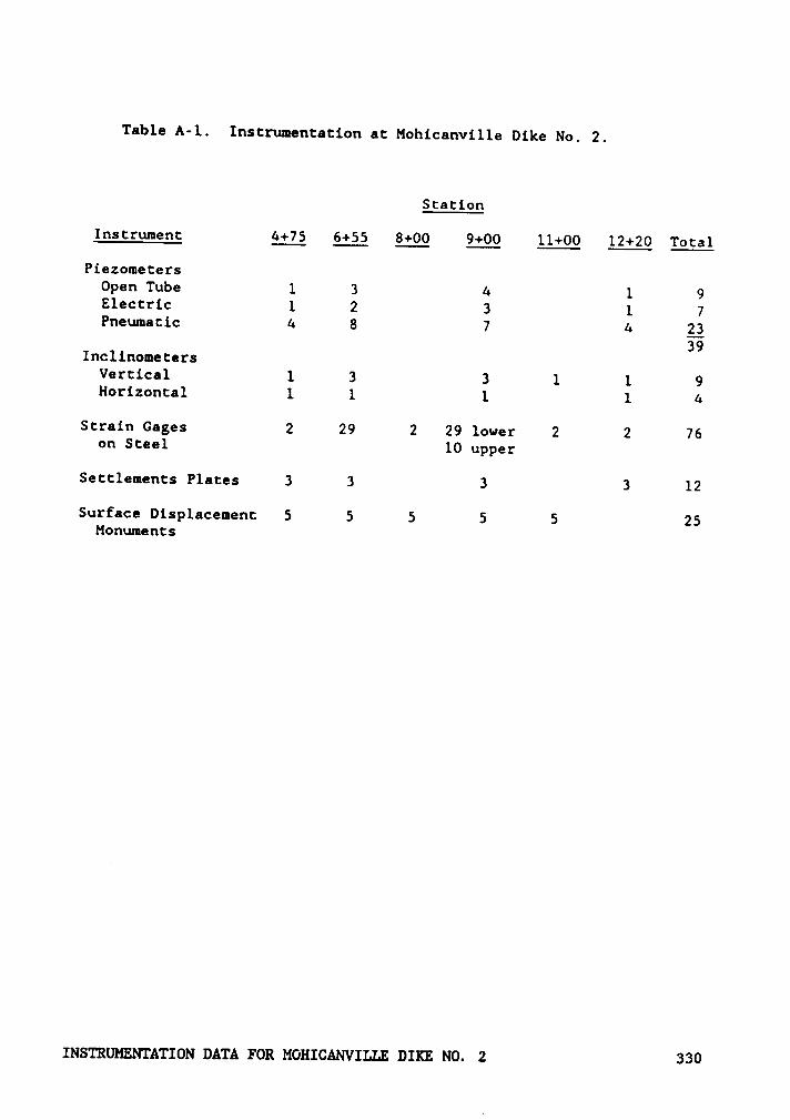
Table A·l. Instrumentation at Mohicanville Dike No. 2.
Station
Instrument &+75 6+55 8+00 9+00 11+00 12+20 Total
PiezometersOpen Tube 1 3 4 l 9Electric 1 2 3 1 7Pneumatic A 8 7 A 22
39InclinometersVertical 1 3 3 1 1 9Horizontal l 1 1 1 6
Strain Gages 2 29 2 29 lower 2 2 76on Steel 10 upper
Settlements Plates 3 3 3 3 12
Surface Displacement 5 S S S 5 25Monuments
INSTRUMENTATION DATA FOR MOHICANVILLE DIKE NO. 2 330

Table A-2. Average crest elevations at instrumented sections.
Sta. Sta. Sta. Sta.Date 4+75 Date 6+55 Date 9+00 Date 12+20
1984
8/10-20 960.0 8/10-20 960.0 9/1-10 960.0 9/5-15 960.08/27-9/20 962.5 8/28-9/20 962.5 9/17-19 961.0 9/21-10/5 961.59/21 963.0 9/21-26 963.0 9/22-10/5 963.5 10/6-9 962.59/26 963.5 9/27 963.5 10/6-15 965.5 10/11 963.010/2 966.5 10/2-4 966.0 10/16 966.7 10/15 966.010/5-16 967.5 10/5-15 966.7 10/18 967.9 10/19 970.010/19 969.0 10/19 969.0 10/23-30 969.0 10/22-31 971.010/23-30 970.0 10/23-30 970.0 11/2 971.0 11/2 972.211/2 971.2 11/2 971.0
1985
6/4 971.2 6/4 971.0 6/4 971.0 6/4 972.26/5-17 972.3 6/5-17 971.8 6/5-17 971.9 6/5-17 973.36/20 973.6 6/20 973.5 6/20 973.2 6/20 974.16/21-25 974.3 6/21 974.6 6/21 974.0 6/25 974.66/27 975.7 6/25 975.7 6/25 975.2 6/26-27 976.26/27-30 977.5 6/27 975.9 6/27 975.4 6/28-30 976.87/1-9 978.3 6/27 977.4 6/27 976.7 7/1-9 979.17/11 979.1 6/28-30 978.4 6/28-30 978.4 7/11 978.27/12-15 979.4 7/1-9 979.6 7/1-9 979.2 7/12-15 981.47/17 981.8 7/11 980.4 7/11 981.3 7/17 982.17/23 982.5 7/12-15 981.2 7/12-15 982.3 7/23 982.77/31 983.0 7/17 982.7 7/17 982.8 7/31 983.29/4 983.04 7/23 983.5 7/23 983.610/7 982.99 7/31 984.0 7/31 984.01/21/86 982.92 9/4 983.94 9/4 983.853/27 982.82 10/7 983.85 10/7 983.71
1/21/86 983.68 1/21/86 983.553/27 983.57 3/27 983.40
Notes: 1. Two measurements on 6/27/85:10:00 an for piezometers6:00 pm for strain gages
2. Elevations for 9/4/85 and after come from surface monumentslocated 5 ft upstream.
INSTRUMENTATION DATA FOR MOHICANVILLE DIKE NO. 2 331

Table A·3. Centerline reinforcement forces (in tons/ft).
Station 4 + 75 Station 6 + 55Date Force Crest Elev. Date Force Crest Elev.
8/27/84 Installed 960.0 8/28/84 Installed 960.09/21 0.31 962.5 9/21 0.30 963.09/26 0.36 963.0 9/26 0.26 963.510/2 1.64 966.5 10/2 1.45 966.010/5 2.23 967.5 10/8 2.14 966.710/8 2.28 967.5 10/11 2.28 966.710/9 2.28 967.5 10/15 2.42 966.710/11 2.31 967.5 10/19 2.63 966.710/15 2.43 967.5 10/23 4.05 969.010/19 3.28 969.0 10/23 4.56 970.010/23 3.82 970.0 10/26 4.67 970.010/26 3.86 970.0 10/30 4.72 970.010/30 4.06 970.0 11/2 . 5.65 971.011/2 4.75 971.2 11/7 5.69 971.011/7 4.78 971.2 11/13 5.68 971.011/13 4.71 971.2 11/19 5.67 971.011/19 4.70 971.2 12/11 5.50 971.0
5/17/85 3.58 971.2 5/16/85 5.27 971.06/7 3.92 972.3 6/7 5.44 972.86/12 3.87 972.3 6/12 5.39 972.86/19 3.97 973.6 6/19 6.60 974.66/24 4.83 974.3 6/24 7.84 976.16/27 6.58 977.5 6/27 9.58 977.46/28 6.90 977.5 6/28 10.51 978.47/1 7.58 978.3 7/1 11.96 979.67/8 7.88 978.3 7/3 12.43 979.67/11 8.19 979.1 7/8 12.83 979.67/15 8.59 979.4 7/9 12.88 979.67/18 9.48 981.8 7/11 13.21 980.47/22 9.73 982.5 7/15 13.69 981.47/25 9.79 982.5 7/18 14.45 982.77/31 9.92 983.0 7/22 14.92 983.58/14 10.29 983.0 7/25 14.89 983.59/5 10.43 983.0 7/31 15.03 984.010/3 10.45 983.0 8/14 15.21 984.012/4 11.71 982.9 9/5 15.27 983.93/12/86 11.84 982.8 10/3 15.28 983.8
12/4 15.22 983.73/12/86 15.27 983.6
Note: Values from upstream gage.
INSTRUMNTATION DATA FOR MOHICANVILLE DIKE NO. 2 332
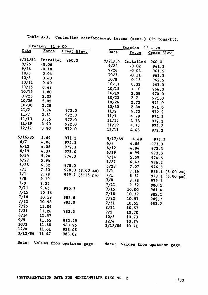
Table A-3. Centerline reinforcement forces (cont.) (in tons/ft).
Station 11 + 00 Station 12 + 20Date Force Crest Elev. Date Force Crest Elev.
9/21/84 Installed 960.0 9/21/84 Installed 960.09/25 -0.06 9/22 -0.02 961.59/26 -0.18 9/26 -0.03 961.510/3 0.04 10/3 -0.11 961.510/8 0.40 10/8 0.13 962.510/11 0.40 10/11 0.32 963.010/15 0.68 10/15 1.10 966.010/19 1.80 10/19 2.59 970.010/23 2.02 10/23 2.71 971.010/26 2.05 10/26 2.72 971.010/30 2.28 10/30 2.88 971.011/2 3.74 972.0 11/2 4.72 972.211/7 3.81 972.0 11/7 4.79 972.211/13 3.85 972.0 11/13 4.73 972.211/19 3.90 972.0 11/19 4.73 972.212/11 3.90 972.0 12/11 4.63 972.2
5/16/85 3.69 971.2 5/17/85 4.48 972.26/7 4.06 972.3 6/7 4.86 973.36/12 4.08 972.3 6/12 4.84 973.36/19 4.37 973.6 6/19 4.99 973.36/24 5.24 974.3 6/24 5.59 974.66/27 5.94 6/27 6.47 976.26/28 6.82 978.0 6/28 7.07 976.87/1 7.30 978.0 (8:00 am) 7/1 7.16 976.8 (8:00 am)7/1 7.78 979.7 (5:15 pm) 7/1 8.31 979.1 (6:00 pm)7/8 9.19 7/8 8.78 979.17/9 9.25 7/11 9.52 980.57/11 9.63 980.7 7/15 10.00 981.47/15 10.36 7/18 10.39 982.17/18 10.59 982.8 7/22 10.51 982.77/22 10.98 983.0 7/31 10.55 983.27/25 11.06 8/14 10.677/31 11.26 983.5 9/5 10.708/14 11.57 10/3 10.739/5 11.65 983.29 12/4 10.7410/3 11.68 983.25 3/12/86 10.7112/4 11.61 983.083/12/86 11.47 983.02
Note: Values from upsttcam gage. Note: Values from upstream gage.
INSTRUMENTATION DATA FOR MOHICANVILLE DIKE NO. 2 333
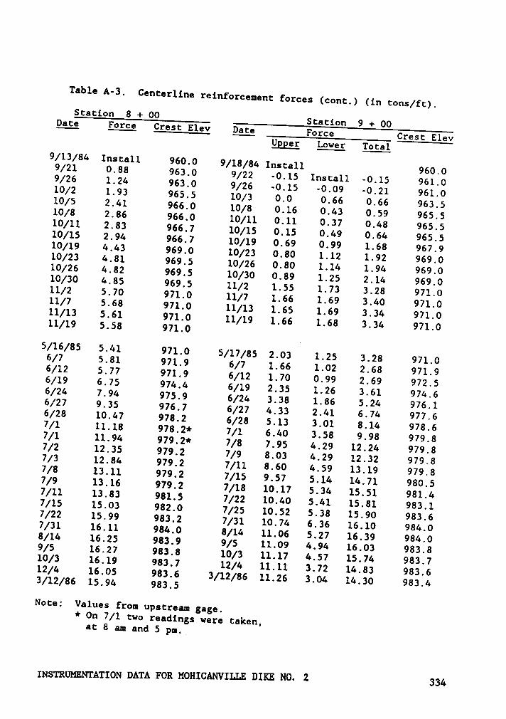
Table A-3. Centerline reinforcement forces (cont.) (in tons/ft).Station 8 + 00
Station 9 + 00Date Force Crest Elev Date Force Crest ElevUgger Lower Total9/13/84 Install 960.0 9/18/84 Install
960.09/21 0.88 963.0 9/22 -0.15 Install -0.15 961.09/26 1.24 963.0 9/26 -0.15 ·0.09 -0.21 961.010/2 1.93 965.5 10/3 0.0 0.66 0.66 963.510/5 2.41 966.0 10/8 0.16 0.43 0.59 965.510/8 2.86 966.0 10/11 0.11 0.37 0.48 965.510/11 2.83 966.7 10/15 0.15 0.49 0.64 965.510/15 2.94 966.7 10/19 0.69 0.99 1.68 967.910/19 4.43 969.0 10/23 0.80 1.12 1.92 969.010/23 4.81 969.5 10/26 0.80 1.14 1.94 969.010/26 4.82 969.5 10/30 0.89 1.25 2.14 969.010/30 4.85 969.5 11/2 1.55 1.73 3.28 971.011/2 5.70 971.0 11/7 1.66 1.69 3.40 971.011/7 5.68 971.0 11/13 1.65 1.69 3.34 971.011/13 5.61 971.0 11/19 1.66 1.68 3.34 971.011/19 5.58 971.0
5/16/85 5.41 971.0 5/17/85 2.03 1.25 3.28 971.06/7 5.81 971.9 6/7 1.66 1.02 2.68 971.96/12 5.77 971.9 6/12 1.70 0.99 2.69 972.56/19 6.75 974.4 6/19 2.35 1.26 3.61 974.66/24 7.94 975.9 6/24 3.38 1.86 5.24 976.16/27 9.35 976.7 6/27 4.33 2.41 6.74 977.66/28 10.47 978.2 6/28 5.13 3.01 8.14 978.67/1 11.18 978.2* 7/1 6.40 3.58 9.98 979.87/1 11.94 979.2* 7/8 7.95 4.29 12.24 979.87/2 12.35 979.2 7/9 8.03 4.29 12.32 979.87/3 12.84 979.2 7/11 8.60 4.59 13.19 979.87/8 13.11 979.2 7/15 9.57 5.14 14.71 980.57/9 13.16 979.2 7/18 10.17 5.34 15.51 981.47/11 13.83 981.5 7/22 10.40 5.41 15.81 983.17/15 15.03 982.0 7/25 10.52 5.38 15.90 983.67/22 15.99 983.2 7/31 10.74 6.36 16.10 984.07/31 16.11 984.0 8/14 11.06 5.27 16.39 984.08/14 16.25 983.9 9/5 11.09 4.94 16.03 983.89/5 16.27 983.8 10/3 11.17 4.57 15.74 983.710/3 16.19 983.7 12/4 11.11 3.72 14.83 983.612/4 16.05 983.6 3/12/86 11.26 3.04 14.30 983.43/12/86 15.94 983.5
Note: Values from upstream gage.* On 7/1 two readings were taken,at 8 am and S pm._
INSTRUMNTATION DATA FOR MOHICANVILLE DIKE N0. 2334
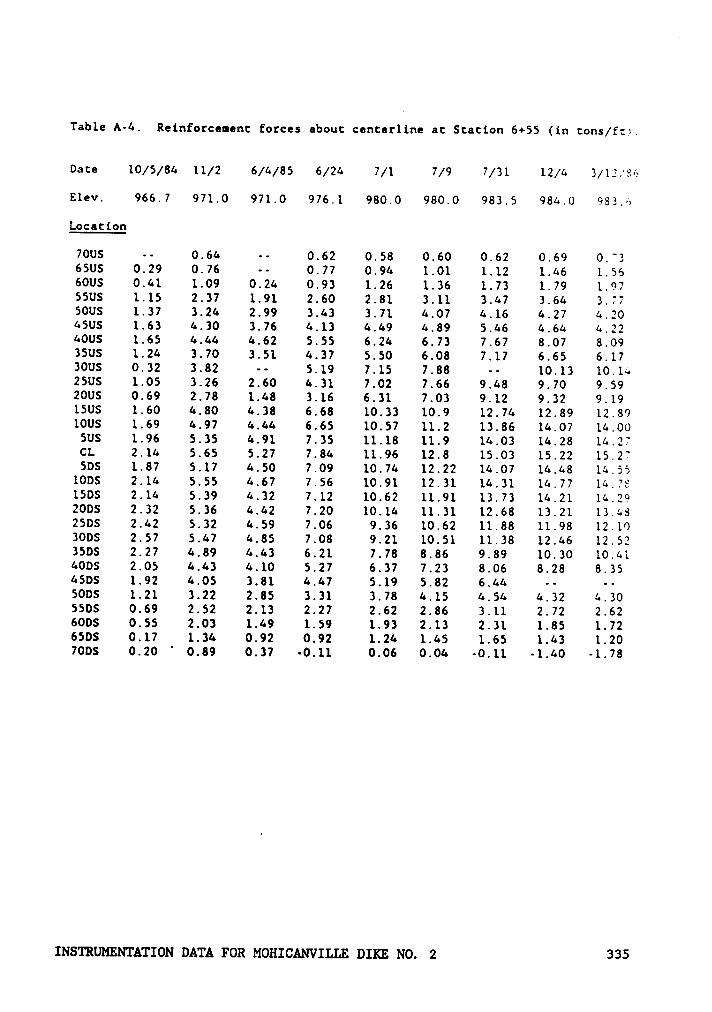
Table A·4. Reinforcement fotces about centerline at Station 6+55 (in tons/ft}.
Date 10/5/84 11/2 6/4/85 6/24 7/1 7/9 7/31 12/4 3/12/86
Elev. 966.7 971.0 971.0 976.1 980.0 980.0 983.5 984.0 953.6
Location
7005 -- 0.64 ~- 0.62 0.58 0.60 0.62 0.69 0.“365US 0.29 0.76 -- 0.77 0.94 1.01 1.12 1.46 1.5660US 0.41 1.09 0.24 0.93 1.26 1.36 1.73 1.79 1.97SSUS 1.15 2.37 1.91 2.60 2.81 3.11 3.47 3.64 3.7750US 1.37 3.24 2.99 3.43 3.71 4.07 4.16 4.27 4.204SUS 1.63 4.30 3.76 4.13 4.49 4.89 5.46 4.64 4.2240US 1.65 4.44 4.62 5.55 6.24 6.73 7.67 8.07 8.0935US 1.24 3.70 3.51 4.37 5.50 6.08 7.17 6.65 6.173005 0.32 3.82 -· 5.19 7.15 7.88 -· 10.13 10.1425US 1.05 3.26 2.60 4.31 7.02 7.66 9.48 9.70 9.592005 0.69 2.78 1.48 3.16 6.31 7.03 9.12 9.32 9.1915US 1.60 4.80 4.38 6.68 10.33 10.9 12.74 12.89 12.8910US 1.69 4.97 4.44 6.65 10.57 11.2 13.86 14.07 14.00
SUS 1.96 5.35 4.91 7.35 11.18 11.9 14.03 14.28 14.27CL 2.14 5.65 5.27 7.84 11.96 12.8 15.03 15.22 15.27SDS 1.87 5.17 4.50 7.09 10.74 12.22 14.07 14.48 14.55
1005 2.14 5.55 4.67 7.56 10.91 12.31 14.31 14.77 14.751505 2.14 5.39 4.32 7.12 10.62 11.91 13.73 14.21 14.292005 2.32 ·5.36 4.42 7.20 10.14 11.31 12.68 13.21 13.4825DS 2.42 5.32 4.59 7.06 9.36 10.62 11.88 11.98 12.103005 2.57 5.47 4.85 7.08 9.21 10.51 11.38 12.46 12.523505 2.27 4.89 4.43 6.21 7.78 8.86 9.89 10.30 10.4140DS 2.05 4.43 4.10 5.27 6.37 7.23 8.06 8.28 8.354505 1.92 4.05 3.81 4.47 5.19 5.82 6.44 -- ·~5005 1.21 3.22 2.85 3.31 3.78 4.15 4.54 4.32 4.305505 0.69 2.52 2.13 2.27 2.62 2.86 3.11 2.72 2.626005 0.55 2.03 1.49 1.59 1.93 2.13 2.31 1.85 1.726505 0.17 1.34 0.92 0.92 1.24 1.45 1.65 1.43 1.207005 0.20
”0.89 0.37 -0.11 0.06 0.04 -0.11 -1.40 -1.78
INSTRUMENTATION DATA FOR MOHICANVILLE DIKE NO. 2 335
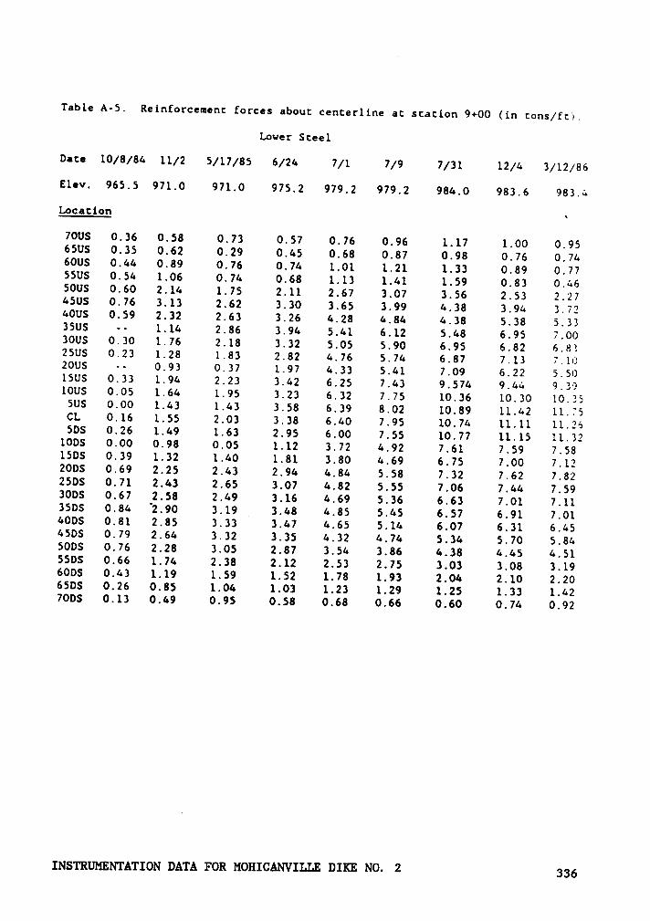
Table A·5. Reinforcement forces about centerline at station 9+00 (in tons/ft)
Lower Steel
Date 10/8/84 11/2 5/17/85 6/24 7/1 7/9 7/31 12/4 3/12/86
Elev. 965.5 971.0 971.0 975.2 979.2 979.2 984.0 983.6 983.4Location ‘7005 0.36 0.58 0.73 0.57 0.76 0.96 1.17 1.00 0.956505 0.35 0.62 0.29 0.45 0.68 0.87 0.98 0.76 0.746005 0.44 0.89 0.76 0.74 1.01 1.21 1.33 0.89 0.775505 0.54 1.06 0.74 0.68 1.13 1.41 1.59 0.83 0.465005 0.60 2.14 1.75 2.11 2.67 3.07 3.56 2.53 2.274505 0.76 3.13 2.62 3.30 3.65 3.99 4.38 3.94 3.724005 0.59 2.32 2.63 3.26 4.28 4.84 4.38 5.38 5.333505 —· 1.14 2.86 3.94 5.41 6.12 5.48 6.95 7.003005 0.30 1.76 2.18 3.32 5.05 5.90 6.95 6.82 6.832505 0.23 1.28 1.83 2.82 4.76 5.74 6.87 7.13 7.102005 -- 0.93 0.37 1.97 4.33 5.41 7.09 6.22 5.501505 0.33 1.94 2.23 3.42 6.25 7.43 9.574 9.44 9.3G1005 0.05 1.64 1.95 3.23 6.32 7.75 10.36 10.30 10.35505 0.00 1.43 1.43 3.58 6.39 8.02 10.89 11.42 11.75CL 0.16 1.55 2.03 3.38 6.40 7.95 10.74 11.11 11.26505 0.26 1.49 1.63 2.95 6.00 7.55 10.77 11.15 11.321005 0.00 0.98 0.05 1.12 3.72 4.92 7.61 7.59 7.581505 0.39 1.32 1.40 1.81 3.80 4.69 6.75 7.00 7.122005 0.69 2.25 2.43 2.94 4.84 5.58 7.32 7.62 7.822505 0.71 2.43 2.65 3.07 4.82 5.55 7.06 7.44 7.593005 0.67 2.58 2.49 3.16 4.69 5.36 6.63 7.01 7.113505 0.84 2.90 3.19 _ 3.48 4.85 5.45 6.57 6.91 7.014005 0.81 2.85 3.33 3.47 4.65 5.14 6.07 6.31 6.454505 0.79 2.64 3.32 3.35 4.32 4.74 5.34 5.70 5.845005 0.76 2.28 3.05 2.87 3.54 3.86 4.38 4.45 4.515505 0.66 1.74 2.38 2.12 2.53 2.75 3.03 3.08 3.196005 0.43 1.19 1.59 1.52 1.78 1.93 2.04 2.10 2.206505 0.26 0.85 1.04 1.03 1.23 1.29 1.25 1.33 1.427005 0.13 0.49 0.95 0.58 0.68 0.66 0.60 0.74 0.92
INSTRUMENTATION DATA FOR MOHICANVILLE DIE NO. 2 336
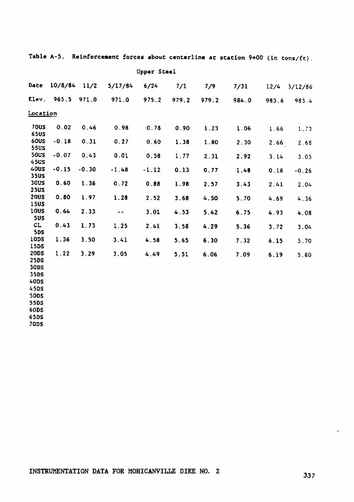
Table A-5. Reinforcement forces about centerline at station 9+00 (in tons/ft).
Upper Steel
Date 10/8/84 11/2 5/17/84 6/24 7/1 7/9 7/31 12/4 3/12/86
Elev. 965.5 971.0 971.0 975.2 979.2 979.2 984.0 983.6 983.4
Location
70US 0.02 0.46 0.98 0.78 0.90 1.23 1.06 1.66 1,7365US60US -0.18 0.31 0.27 0.60 1.38 1.80 2.30 2.66_ 2.6855US50US -0.07 0.43 0.01 0.58 1.77 2.31 2.92 3.14 3.0545US40US -0.15 -0.30 -1.48 -1.12 0.13 0.77 1.48 0.18 -0.2635US30US 0.60 1.36 0.72 0.88 1.98 2.57 3.43 2.41 2.0425US20US 0.80 1.97 1.28 2.52 3.68 4.50 5.70 4.69 4.3615U510U5 0.64 2.33 -· 3.01 4.53 5.42 6.75 4.93 4.08
SU5CL 0.43 1.73 1.25 2.41 3.58 4.29 5.36 3.72 3.04505
1005 1.36 3.50 3.41 4.58 5.65 6.30 7.32 6.15 5.7015052005 1.22 3.29 3.05 4.49 5.51 6.06 7.09 6.19 5.802505300535054005450550055505600565057005
INSTRUMENTATION DATA FOR MOHICANVILLE DIKE NO. 2 337
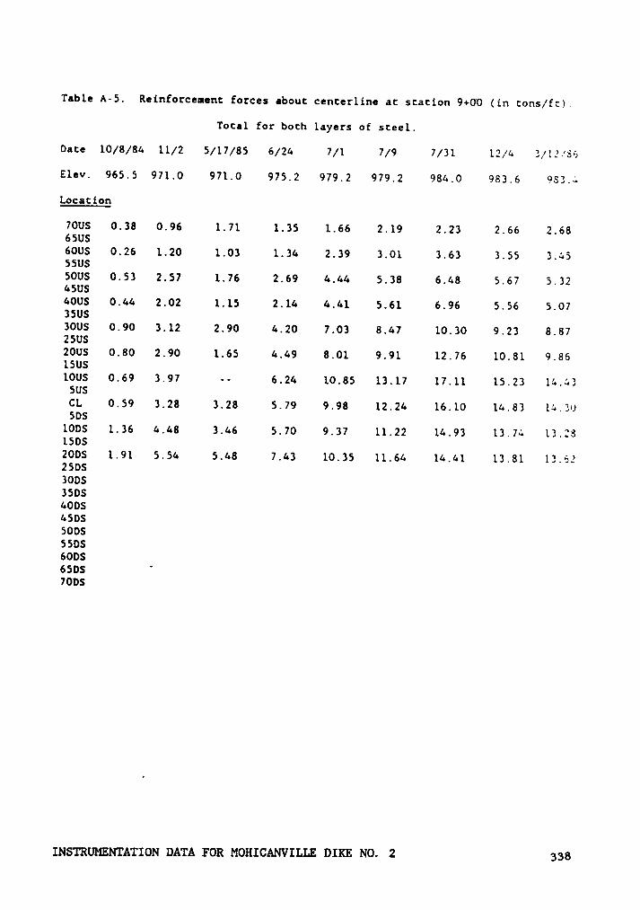
Table A-5. Reinforcement fotces about centerline at station 9+00 (in tons/ft)
Total for both layers of steel.
Date 10/8/84 11/2 5/17/85 6/24 7/1 7/9 7/31 12/4 3/12/S6
Elev. 965.5 971.0 971.0 975.2 979.2 979.2 984.0 983.6 983.4
Location
7005 0.38 0.96 1.71 1.35 1.66 2.19 2.23 2.66 2.6865US60U5 0.26 1.20 1.03 1.34 2.39 3.01 3.63 3.55 3.4555US50U5 0.53 2.57 1.76 2.69 4.44 5.38 6.48 5.67 5.32450540U5 0.44 2.02 1.15 2.14 4.41 5.61 6.96 5.56 5.0735U530U5 0.90 3.12 2.90 4.20 7.03 8.47 10.30 9.23 8.8725US20U5 0.80 2.90 1.65 4.49 8.01 9.91 12.76 10.81 9.8615US10U5 0.69 3.97 ~- 6.24 10.85 13.17 17.11 15.23 14.435U5CL 0.59 3.28 3.28 5.79 9.98 12.24 16.10 14.83 14.30505
1005 1.36 4.48 3.46 5.70 9.37 11.22 14.93 13.74 13.2815052005 1.91 5.54 5.48 7.43 10.35 11.64 14.41 13.81 13.62250530053505400545055005550560056505 '7005
INSTRUMENTATION DATA FOR MOHICANVILLE DIE NO. 2 338
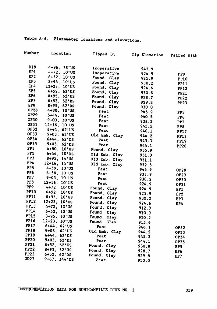
Table A-6. Piezometer locations and elevations.
Number Location Tipped In Tip Elevation Paired With
D18 4+96, 78'US Inoperative 945.9EP1 4+72, 10'US Inoperative 924.9 PP9EP2 6+52, 10'US Found. Clay 925.9 PP1OEP3 8+95, 10'US Found. Clay 930.2 PP11EP4 12+23, 10'US Found. Clay 924.6 PP12EP5 6+52, 62'US Found. Clay 930.8 PP21EP6 8+95, 62'US Found. Clay 928.7 PP22EP7 6+52, 62'DS Found. Clay 929.8 PP23EP8 8+95, 62'DS Found. Clay 930.0
OP28 4+80, 10'US Peat 945.9 PP5OP29 6+44, 10'US Peat 940.5 PP6OP30 9+03, 10'US Peat 938.2 PP7OP3l 12+16, 10'US Peat 945.5 PP8OP32 6+44, 62'US Peat 946.1 PP17OP33 9+03, 62'US Old Emb. Clay 944.2 PP18OP34 6+44, 62'DS Peat 945.3 PP19OP35 9+03, 62'DS Peat 944.1 PP20PP1 4+80, 10'US Found. Clay 935.9PP2 6+44, 10'US Old Emb. Clay 951.0PP3 8+95, 14'US Old Emb. Clay 951.1PP4 12+16, 14'US Old Emb. Clay 952.5PP5 4+59, 10'US Peat 945.9 OP28PP6 6+58, 10'US Peat 938.9 OP29PP7 9+03, 10'US Peat 938.2 OP30PP8 12+16, 10'US Peac 924.9 OP3lPP9 4+72, 10'US Found. Clay _ 924.9 EP1PPl0 6+52, 10'US Found. Clay 925.9 EP2PP11 8+95, 10'US Found. Clay 930.2 EP3PP12 12+23, 10'US Found. Clay 924.6 EP4PP13 4+72, 10'US Found. Clay 912.9PPl4 6+52, 10'US Found. Clay 910.9PPl5 8+95, 10'US Found. Clay 910.2PPl6 12+23, 10'US Found. Clay 915.6PP17 6+44, 62'US Peat 946.1 OP32PP18 9+03, 62'US Old Emb. Clay 944.2 OP33PP19 6+44, 62'DS Peat 945.3 OP34PP20 9+03, 62'DS Peat 944.1 OP35PP21 6+52, 62'US Found. Clay 930.8 EP5PP22 8+95, 62•us Found. Clay 928.7 EP6PP23 6+52, 62'DS Found. Clay 929.8 EP7UD27 9+67, 144'DS Peat 950.0
INSTRUMNTATION DATA FOR MOHICANVILLE DIKE NO. 2 339
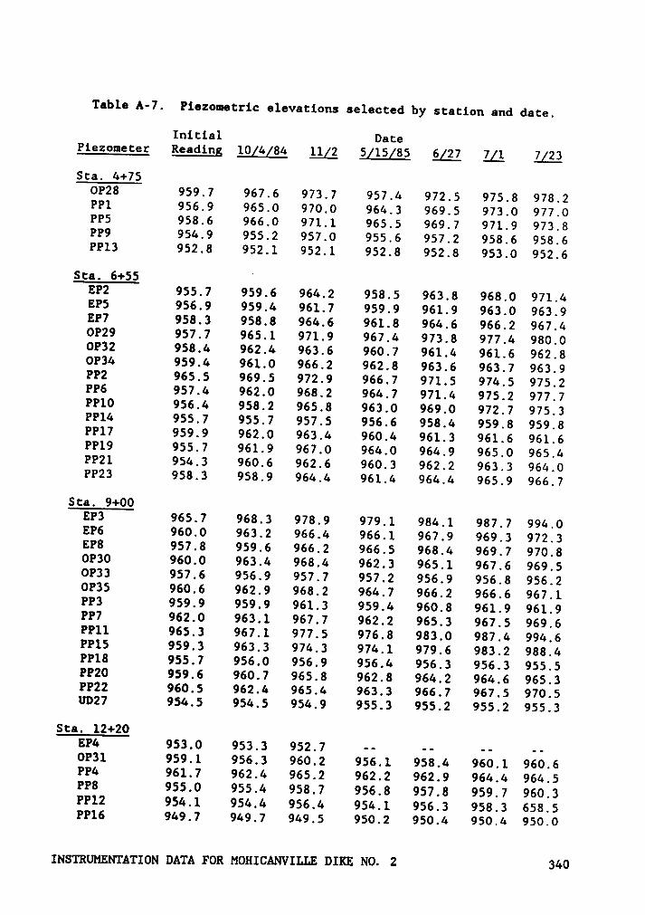
Table A·7. Piezomettic elevations selected by station and date.
Initial DatePiezometer Reading 10g4g84 1lg2 5g1Sg85 6g27 lll 7g23Sta. 4+75
OP28 959.7 967.6 973.7 957.4 972.5 975.8 978.2PP1 956.9 965.0 970.0 964.3 969.5 973.0 977.0PP5 958.6 966.0 971.1 965.5 969.7 971.9 973.8PP9 954.9 955.2 957.0 955.6 957.2 958.6 958.6PP13 952.8 952.1 952.1 952.8 952.8 953.0 952.6Sta. 6+55 ”
EP2 955.7 959.6 964.2 958.5 963.8 968.0 971.4EPS 956.9 959.4 961.7 959.9 961.9 963.0 963.9EP7 958.3 958.8 964.6 961.8 964.6 966.2 967.4OP29 957.7 965.1 971.9 967.4 973.8 977.4 980.0OP32 958.4 962.4 963.6 960.7 961.4 961.6 962.8OP34 959.4 961.0 966.2 962.8 963.6 963.7 963.9PP2 965.5 969.5 972.9 966.7 971.5 974.5 975.2PP6 957.4 962.0 968.2 964.7 971.4 975.2 977.7PP10 956.4 958.2 965.8 963.0 969.0 972.7 975.3PPl4 955.7 955.7 957.5 956.6 958.4 959.8 959.8PP17 959.9 962.0 963.4 960.4 961.3 961.6 961.6PP19 955.7 961.9 967.0 964.0 964.9 965.0 965.4PP21 954.3 960.6 962.6 960.3 962.2 963.3 964.0PP23 958.3 958.9 964.4 961.4 964.4 965.9 966.7Sta. 9+00
EP3 965.7 968.3 978.9 979.1 984.1 987.7 994.0EP6 960.0 963.2 966.4 966.1 967.9 969.3 972.3EP8 957.8 959.6 966.2 966.5 968.4 969.7 970.8OP30 960.0 963.4 968.4 962.3 965.1 967.6 969.5OP33 957.6 956.9 957.7 957.2 956.9 956.8 956.2OP35 960.6 962.9 968.2 964.7 966.2 966.6 967.1PP3 959.9 959.9 961.3 959.4 960.8 961.9 961.9PP7 962.0 963.1 967.7 962.2 965.3 967.5 969.6PP11 965.3 967.1 977.5 976.8 983.0 987.4 994.6PP1S 959.3 963.3 974.3 974.1 979.6 983.2 988.4PP18 955.7 956.0 956.9 956.4 956.3 956.3 955.5PP20 959.6 960.7 965.8 962.8 964.2 964.6 965.3PP22 960.5 962.4 965.4 963.3 966.7 967.5 970.5UD27 954.5 954.5 954.9 955.3 955.2 955.2 955.3Sta. 12+20
EP4 953.0 953.3 952.7 -· ·· —· —·OP31 959.1 956.3 960.2 956.1 958.4 960.1 960.6PP4 961.7 962.4 965.2 962.2 962.9 964.4 964.5PP8 955.0 955.4 958.7 956.8 957.8 959.7 960.3PPl2 954.1 954.4 956.4 954.1 956.3 958.3 658.5PP16 949.7 949.7 949.5 950.2 950.4 950.4 950.0
INSTRUMENTATION DATA FOR MOHICANVILLE DIKE NO. 2 340
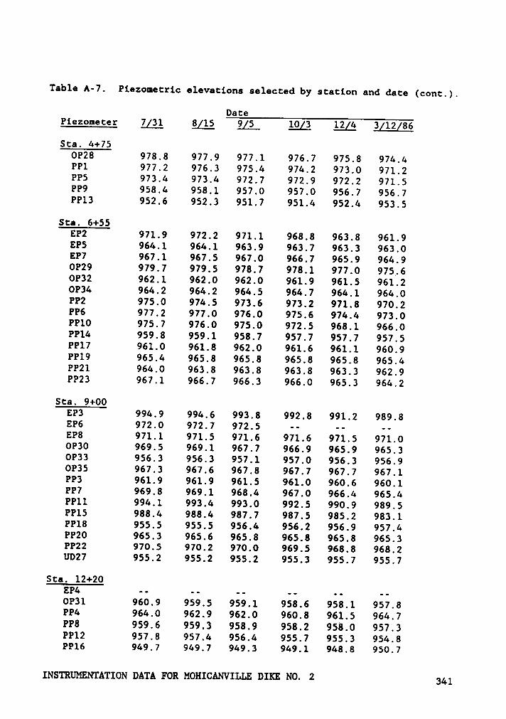
Table A·7. Piezometric elevations selected by station and date (cont.).
DatePiezometer 7[31 8glS 9gS 10[3 12g4 3g12g86
Sta. 4+75OP28 978.8 977.9 977.1 976.7 975.8 974.4PP1 977.2 976.3 975.4 974.2 973.0 971.2PP5 973.4 973.4 972.7 972.9 972.2 971.5PP9 958.4 958.1 957.0 957.0 956.7 956.7PP13 952.6 952.3 951.7 951.4 952.4 953.5
Sta. 6+55EP2 971.9 972.2 971.1 968.8 963.8 961.9EP5 964.1 964.1 963.9 963.7 963.3 963.0EP7 967.1 967.5 967.0 966.7 965.9 964.9OP29 979.7 979.5 978.7 978.1 977.0 975,6OP32 962.1 962.0 962.0 961.9 961.5 961.2OP34 964.2 964.2 964.5 964.7 964.1 964.0PP2 975.0 974.5 973.6 973.2 971.8 970.2PP6 977.2 977.0 976.0 975.6 974.4 973.0PP10 975.7 976.0 975.0 972.5 968.1 966.0PP14 959.8 959.1 958.7 957.7 957.7 957.5PP17 961.0 961.8 962.0 961.6 961.1 960.9PP19 965.4 965.8 965.8 965.8 965.8 965.4PP21 964.0 963.8 963.8 963.8 963.3 962.9PP23 967.1 966.7 966.3 966.0 965.3 964.2
Sta. 9+00EP3 994.9 994.6 993.8 992.8 991.2 989.8EP6 972.0 972.7 972.5 ·· -· -·EP8 971.1 971.5 971.6 971.6 971.5 971.0OP30 969.5 969.1 967.7 966.9 965.9 965.3OP33 956.3 956.3 957.1 957.0 956.3 956.9OP35 967.3 967.6 967.8 967.7 967.7 967.1PP3 961.9 961.9 961.5 961.0 960.6 960.1PP7 969.8 969.1 968.4 967.0 966.4 965.4PP11 994.1 993.4 993.0 992.5 990.9 989.5PP15 988.4 988.4 987.7 987.5 985.2 983.1PP18 955.5 955.5 956.4 956.2 956.9 957.4PP20 965.3 965.6 965.8 965.8 965.8 965.3PP22 970.5 970.2 970.0 969.5 968.8 968.2UD27 955.2 955.2 955.2 955.3 955.7 955.7
Sta. 12+20EP4 -- -- -· -· •· •·OP31 960.9 959.5 959.1 958.6 958.1 957.8PP4 964.0 962.9 962.0 960.8 961.5 964.7PP8 959.6 959.3 958.9 958.2 958.0 957.3PP12 957.8 957.4 956.4 955.7 955.3 954.8PP16 949.7 949.7 949.3 949.1 948.8 950.7
INSTRUMENTATION DATA FOR MOHICANVILLE DIKE NO. 2 341
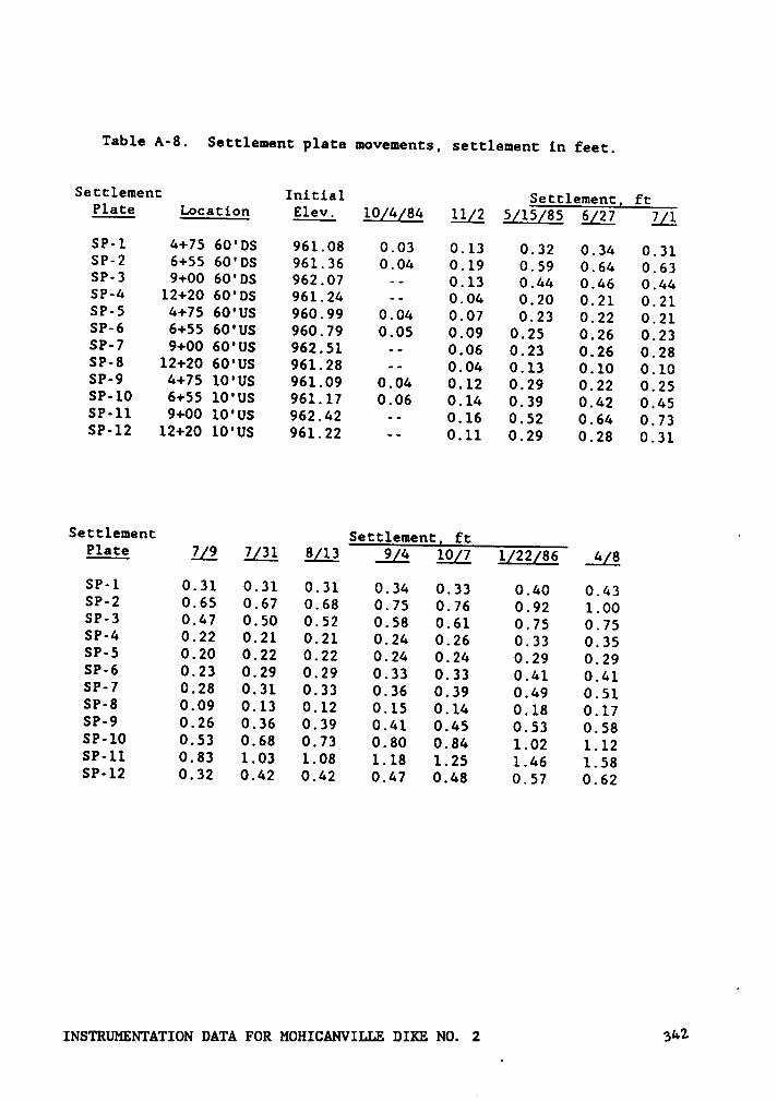
Table A-8. Settlement plate movements, settlement in feet.
Settlement Initial Settlement! ftPlate Location Elev. 10[4[84 11[2 5[15[85 6[27 [[1
SP-1 4+75 60'DS 961.08 0.03 0.13 0.32 0.34 0.31SP—2 6+55 60'DS 961.36 0.04 0.19 0.59 0.64 0.63SP·3 9+00 60'DS 962.07 -· 0.13 0.44 0.46 0.44SP-4 12+20 60'DS 961.24 -· 0.04 0.20 0.21 0.21SP-5 4+75 60'US 960.99 0.04 0.07 0.23 0.22 0.21SP-6 6+55 60'US 960.79 0.05 0.09 0.25 0.26 0.23SP·7 9+00 60'US 962.51 -- 0.06 0.23 0.26 0.28SP·8 12+20 60'US 961.28 ·- 0.04 0.13 0.10 0.10SP·9 4+75 10'US 961.09 0.04 0.12 0.29 0.22 0.25SP-10 6+55 10'US 961.17 0.06 0.14 0.39 0.42 0.45SP·l1 9+00 10'US 962.42 -- 0.16 0.52 0.64 0.73SP-12 12+20 10'US 961.22 ·- 0.11 0.29 0.28 0.31
Settlement Settlement. ft ”Plate Z[2 7[31 $[13 9[4 10[7 1[22[86 4[8
SP·1 0.31 0.31 0.31 0.34 0.33 0.40 0.43SP·2 0.65 0.67 0.68 0.75 0.76 0.92 1.00SP·3 0.47 0.50 0.52 0.58 0.61 0.75 0.75SP~4 0.22 0.21 0.21 0.24 0.26 0.33 0.35SP-5 0.20 0.22 0.22 0.24 0.24 0.29 0.29SP-6 0.23 0.29 0.29 0.33 0.33 0.41 0.41SP-7 0.28 0.31 0.33 0.36 0.39 0.49 0.51SP·8 0.09 0.13 0.12 0.15 0.14 0.18 0.17SP·9 0.26 0.36 0.39 0.41 0.45 0.53 0.58SP-10 0.53 0.68 0.73 0.80 0.84 1.02 1.12SP-11 0.83 1.03 1.08 1.18 1.25 1.46 1.58SP·12 0.32 0.42 0.42 0.47 0.48 0.57 0.62
INSTRUMNTATION DATA FOR MOHICANVILLE DIKE NO. 23“2

Table A-9. Elevations of surface displacement monument by date.
Monument Elevation on6 Location Initial 11g8 $[16 7gl 7g31 10[9 146 3g27
0-1 6+75 30'DS 975.21 75.18 75.09 75.090-2 6+75 105'DS 958.80 58.79 58.80 58.78 58.80 58.76 58.83 58.960-3 6+55 30'DS 976.96 76.86 76.66 76.560-6 6+55 105'DS 958.61 58.59 58.58 58.57 58.61 58.57 58.65 58.750-5 7+50 30'DS 976.83 76.76 76.58 76.520-6 7+50 105'DS 957.93 57.90 57.86 57.83 57.86 57.83 57.96 58.020-7 9+00 30'DS 976.91 76.86 76.63 76.500-8 9+00 105'DS 961.60 61.39 61.30 61.31 61.37 61.31 61.33 61.370-9 11+00 30'DS 975.56 75.69 75.35 75.280-10 11+00 105*05 959.00 59.00 58.97 58.97 59.00 59.00 59.02 59.06U-1 6+75 5'US 983.06 82.99 82.92 82.82U·2 6+75 30'US 975.57 75.53 75.65 75.62U-3 6+75 105'U$ 966.86 66.86 66.80 66.79 66.79 66.78 66.78 66.88U-6 6+55 5'US 983.96 83.85 83.68 83 57U•5 6+55 30'US 975.37 75.31 55.16 75.11U-6 6+55 105'US 962.63 62.66 62.68 62.69 62.71 62.71 62.75 62.81U-7 7+50 5'US 983.26 83.18 82 99 82.91U-8 7+50 30'US 975.66 75.39 75.25 75.18U·9 7+50 105'US 962.78 62.79 62.76 62.77 62.80 62.82 62.87 62.96U-10 9+00 · 5'US 983.85 83.77 83.55 83.61U·11 9+00 30'US 975.59 75.53 75.36 75.26U-12 9+00 105'U$ 961.22 61.22 61.17 61.18 61.18 61.18 61.26 61.37U·13 11+00 5'US 983.29 83.25 83.08 83.02U-16 11+00 30'US 976.76 76.72 76.59 76.55U-15 11+00 105'US 962.60 62.61 62.57 62.59 62.59 62.60 62.60 62.61
INSTRUMENTATION DATA FOR MOHICANVILLE DIKE NO. 2 363

Table A-10. Inclinometer information.
Number Location Direction Elevation Initial Reading
1-1 6+62, ll7' US Vertical 961.04 10/13/841-4* 9+42, 85' DS Vertical 962.76I-5 6+87, l03' DS Vertical 958.24 10/ 5/841-6 12+03, l28' US Vertical 958.89 10/ 9/841-7 6+52, 60' US Vertical 967.04 10/ 3/841-8 9+03, 60' US Vertical 970.92 (10/23) 10/18/84
967.67 (6/20/85)1-9 9+03, 4l' US Vertical 974.00 10/18/841-10 4+75, 93° US Horizontal 959.25 9/27/841-11 6+55, 93' US Horizontal 959.26 9/27/841-12 9+00, 93' US Horizontal 959.25 10/ 8/841-13 12+20, 93' US Horizontal 959.21 10/11/841-14 9+14, 150' US Vertical 961.32 6/ 5/851-15* 9+50, 102' DS Vertical 959.10 6/17/85
* 1-4 was destroyed in June, 1985 and replaced with 1-15.
INSTRUMENTATION DATA FOR MOHICANVILLE DIKE NO. 2 344
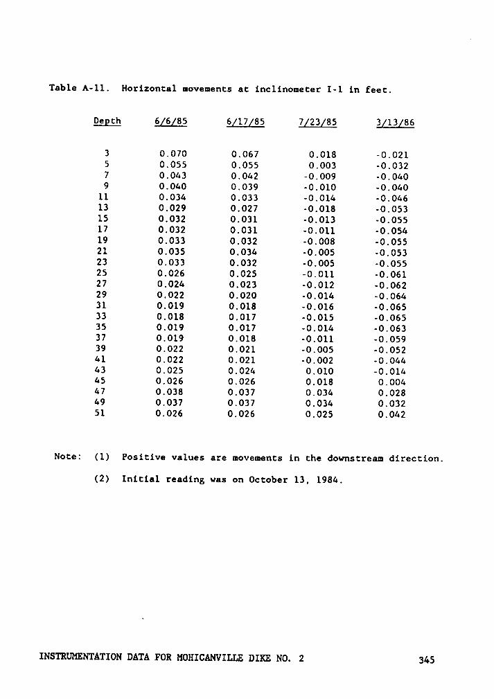
Table A-11. Horizontal movements at inclinometer I-1 in feet.
Degth 6g6g85 6[17g85 7g23g85 3g13g86
3 0.070 0.067 0.018 -0.0215 0.055 0.055 0.003 -0.0327 0.043 0.042 -0.009 -0.0409 0.040 0.039 -0.010 -0.040
11 0.034 0.033 -0.014 -0.04613 0.029 0.027 -0.018 -0.05315 0.032 0.031 -0.013 -0.05517 0.032 0.031 -0.011 -0.05419 0.033 0.032 -0.008 -0.05521 0.035 0.034 -0.005 -0.05323 0.033 0.032 -0.005 -0.05525 0.026 0.025 -0.011 -0.06127 0.024 0.023 -0.012 -0.06229 0.022 0.020 -0.014 -0.06431 0.019 0.018 -0.016 -0.06533 0.018 0.017 -0.015 -0.06535 0.019 0.017 -0.014 -0.06337 0.019 0.018 -0.011 -0.05939 0.022 0.021 -0.005 -0.05241 0.022 0.021 -0.002 ~0.04443 0.025 0.024 0.010 -0.01445 0.026 0.026 0.018 0.00447 0.038 0.037 0.034 0.02849 0.037 0.037 0.034 0.03251 0.026 0.026 0.025 0.042
Note: (1) Positive values are movements in the downstream direction.
(2) Initial reading was on October 13, 1984.
INSTRUMENTATION DATA FOR MOHICANVILLE DIKE NO. 2 345
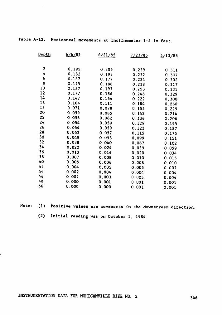
Table A-12. Horizontal movements at inclinometer I-5 in feet.
Degth 6g6g85 6g21[85 7g23g85 3g13g86
2 0.195 0.205 0.239 0.3114 0.182 0.193 0.232 0.3076 0.167 0.177 0.224 0.3028 0.175 0.186 0.238 0.317
10 0.187 0.197 0.253 0.33512 0.177 0.186 0.248 0.32914 0.147 0.154 0.222 0.30016 0.104 0.111 0.184 0.26018 0.071 0.078 0.155 0.22920 0.059 0.065 0.142 0.21422 0.056 0.062 0.136 0.20624 0.054 0.059 0.129 0.19526 0.054 0.059 0.123 0.18728 0.053 0.057 0.115 0.17530 0.049 0.053 0.099 0.15132 0.038 0.040 0.067 0.10234 0.022 0.024 0.039 0.05936 0.013 0.014 0.020 0.03438 0.007 0.008 0.010 0.01540 0.005 0.006 0.008 0.01042 0.004 0.005 0.005 0.00744 0.002 0.004 0.004 0.00446 0.002 0.003 0.003 0.00448 0.000 0.001 0.001 0.00150 0.000 0.000 0.001 0.001
Note: (1) Positive values are movements in the downstream direction.
(2) Initial reading was on October 5, 1984.
INSTRUMNTATION DATA FOR MOHICANVILLE DIKE NO. 2 345
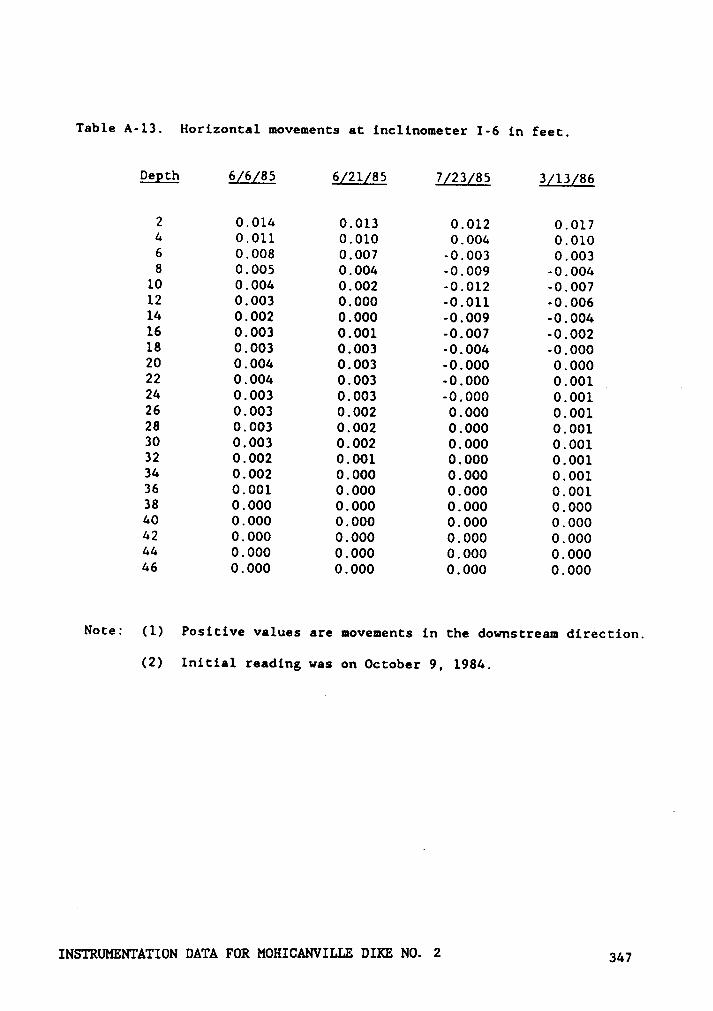
Table A-13. Horizontal movements at inclinometer I-6 in feet.
Degth 6g6g85 6g2lg8S 7g23g8S 3g13g86
2 0.014 0.013 0.012 0.0174 0.011 0.010 0.004 0.0106 0.008 0.007 ·0.003 0.0038 0.005 0.004 -0.009 -0.004
10 0.004 0.002 -0.012 -0.00712 0.003 0.000 -0.011 -0.00614 0.002 0.000 -0.009 -0.00416 0.003 0.001 -0.007 -0.00218 0.003 0.003 -0.004 -0.00020 0.004 0.003 -0.000 0.00022 0.004 0.003 -0.000 0.001 .24 0.003 0.003 -0.000 0.00126 0.003 0.002 0.000 0.00128 0.003 0.002 0.000 0.00130 0.003 0.002 0.000 0.00132 0.002 0.001 0.000 0.00134 0.002 0.000 0.000 0.00136 0.001 0.000 0.000 0.00138 0.000 0.000 0.000 0.00040 0.000 0.000 0.000 0.00042 0.000 0.000 0.000 0.00044 0.000 0.000 0.000 0.00046 0.000 0.000 0.000 0.000
Note: (1) Positive values are movements in the downstream direction.
(2) Initial reading was on October 9, 1984.
INSTRUMENTATION DATA FOR MOHICANVILLE DIKE NO. 2 gg;
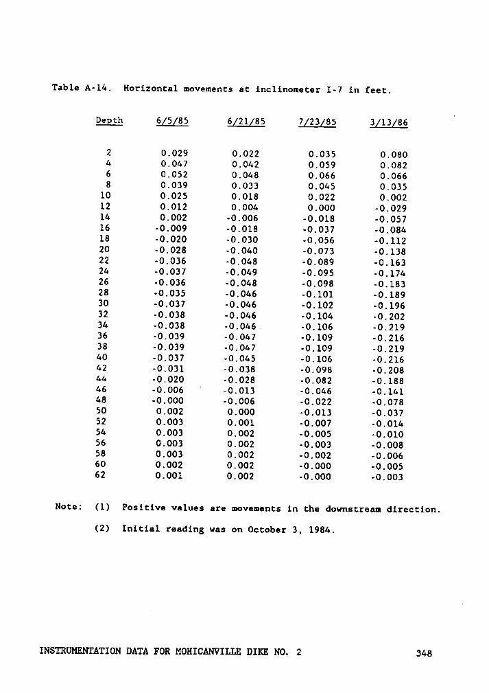
Table A-14. Horizontal movements at inclinometer I-7 in feet.
Degth 6[5[85 6(21g85 7g23g85 3g13g86
2 0.029 0.022 0.035 0.0804 0.047 0.042 0.059 0.0826 0.052 0.048 0.066 0.0668 0.039 0.033 0.045 0.035
10 0.025 0.018 0.022 0.00212 0.012 0.004 0.000 -0.02914 0.002 -0.006 -0.018 -0.05716 -0.009 -0.018 -0.037 -0.08418 -0.020 -0.030 -0.056 -0.11220 -0.028 -0.040 -0.073 -0.13822 -0.036 -0.048 -0.089 -0.16324 -0.037 -0.049 -0.095 -0.17426 -0.036 -0.048 -0.098 -0.18328 -0.035 -0.046 -0.101 -0.18930 -0.037 -0.046 -0.102 -0.19632 -0.038 -0.046 -0.104 -0.20234 -0.038 -0.046 -0.106 -0.21936 -0.039 -0.047 -0.109 -0.21638 -0.039 -0.047 -0.109 -0.21940 -0.037 -0.045 -0.106 -0.21642 -0.031 -0.038 -0.098 -0.20844 -0.020 -0.028 -0.082 -0.18846 -0.006
”-0.013 -0.046 -0.141
48 -0.000 -0.006 -0.022 -0.07850 0.002 0.000 -0.013 -0.03752 0.003 0.001 -0.007 -0.01454 0.003 0.002 -0.005 -0.01056 0.003 0.002 -0.003 -0.00858 0.003 0.002 -0.002 -0.00660 0.002 0.002 -0.000 -0.00562 0.001 0.002 -0.000 -0.003
Note: (1) Positive values are movements in the downstream direction.
(2) Initial reading was on October 3, 1984.
INSTRUMENTATION DATA FOR MOHICANVILLE DIKE NO. 2 348
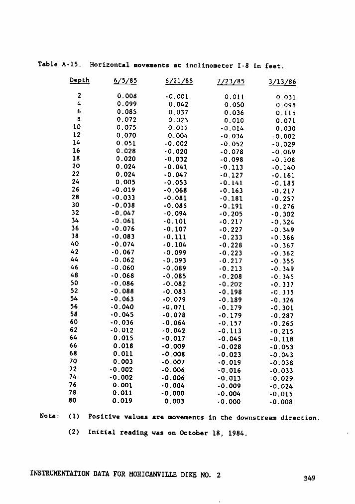
Table A-15. Horizontal movements at inclinometer I-8 in feet.
Degth 6g5g85 6g2lg85 7g23g85 3g13g86
2 0.008 -0.001 0.011 0.0316 0.099 0.062 0.050 0.0986 0.085 0.037 0.036 0.1158 0.072 0.023 0.010 0.071
10 0.075 0.012 -0.016 0.03012 0.070 0.006 -0.036 -0.00216 0.051 -0.002 -0.052 -0.02916 0.028 -0.020 -0.078 -0.06918 0.020 -0.032 -0.098 -0.10820 0.026 -0.061 -0.113 -0.16022 0.026 -0.067 -0.127 -0.16126 0.005 -0.053 -0.161 -0.18526 -0.019 -0.068 -0.163 -0.21728 -0.033 -0.081 -0.181 -0.25730 -0.038 -0.085 -0.191 -0.27632 -0.067 -0.096 -0.205 -0.30236 -0.061 -0.101 -0.217 -0.32636 -0.076 -0.107 -0.227 -0.36938 -0.083 -0.111 -0.233 -0.36660 -0.076 -0.106 -0.228 -0.36762 -0.067 -0.099 -0.223 -0.36266 -0.062 -0.093 -0.217 -0.35566 -0.060 -0.089 -0.213 -0.36968 -0.068 -0.085 -0.208 -0.36550 -0.086 -0.082 -0.202 -0.33752 -0.088 -0.083 -0.198 -0.33556 -0.063 -0.079 -0.189 -0.32656 -0.060 -0.071 -0.179 -0.30158 -0.065 -0.078 -0.179 -0.28760 -0.036 -0.066 -0.157 -0.26562 -0.012 -0.062 -0.113 -0.21566 0.015 -0.017 -0.065 -0.11866 0.018 -0.009 -0.028 -0.05368 0.011 -0.008 -0.023 -0.06370 0.003 -0.007 -0.019 -0.03872 -0.002 -0.006 -0.016 -0.03376 -0.002 -0.006 -0.013 -0.02976 0.001 -0.006 -0.009 -0.02678 0.011 -0.000 -0.006 -0.01580 0.019 0.003 -0.000 -0.008
Note: (1) Positive values are movements in the downstream direction.
(2) Initial reading was on October 18, 1986. '
INSTRUMENTATION DATA FOR MOHICANVILLE DIKE NO. 2 349
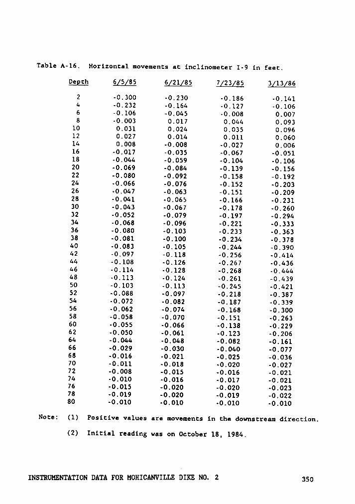
Table A-16. Horizontal movements at inclinometer I-9 in feet.
Degth 6g5g85 6g21g85 7g23g85 3g13g86
2 -0.300 -0.230 -0.186 -0.1414 -0.232 -0.164 -0.127 -0.1066 -0.106 -0.045 -0.008 0.0078 -0.003 0.017 0.044 0.093
10 0.031 0.024 0.035 0.09612 0.027 0.014 0.011 0.06014 0.008 -0.008 -0.027 0.00616 -0.017 -0.035 -0.067 -0.05118 -0.044 -0.059 -0.104 -0.10620 -0.069 -0.084 -0.139 -0.15622 -0.080 -0.092 -0.158 -0.19224 -0.066 -0.076 -0.152 -0.20326 -0.047 -0.063 -0.151 -0.20928 -0.041 -0.065 -0.166 -0.23130 -0.043 -0.067 -0.178 -0.26032 -0.052 -0.079 -0.197 -0.29434 -0.068 -0.096 -0.221 -0.33336 -0.080 -0.103 -0.233 -0.36338 -0.081 -0.100 -0.234 -0.37840 -0.083 -0.105 -0.244 -0.39042 -0.097 -0.118 -0.256 -0.41444 -0.108 -0.126 -0.267 -0.43646 -0.114 -0.128 -0.268 -0.44448 -0.113 -0.124 -0.261 -0.43950 -0.103 -0.113 -0.245 -0.42152 -0.088 -0.097 -0.218 -0.38754 -0.072 -0.082 -0.187 -0.33956 -0.062 -0.074 -0.168 -0.30058 -0.058 -0.070 -0.151 -0.26360 -0.055 -0.066 -0.138 -0.22962 -0.050 -0.061 -0.123 -0.20664 -0.044 -0.048 -0.082 -0.16166 -0.029 -0.030 -0.040 -0.07768 -0.016 -0.021 -0.025 -0.03670 -0.011 -0.018 -0.020 -0.02772 -0.008 -0.015 -0.016 -0.02174 -0.010 -0.016 -0.017 -0.02176 -0.015 -0.020 -0.020 -0.02378 -0.019 -0.020 -0.019 -0.02280 -0.010 -0.010 -0.010 -0.010
Note: (1) Positive values are movements in the downstream direction.
(2) Initial reading was on October 18, 1984.
INSTRUMENTATION DATA FOR MOHICANVILLE DIKE NO. 2 359
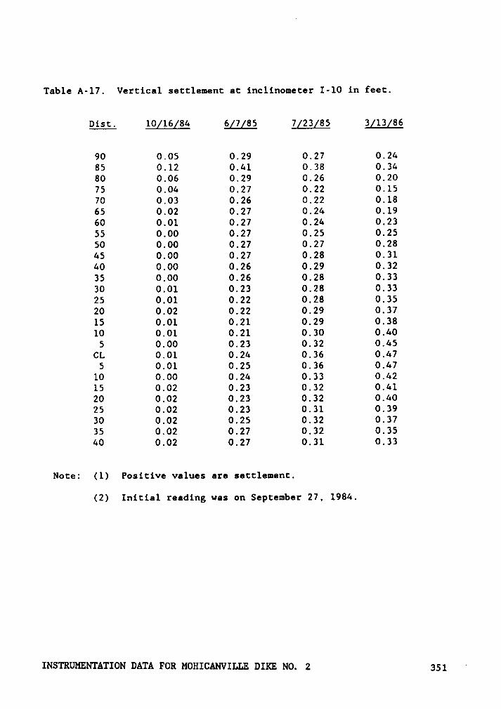
Table A·l7. Vertical setclement ac inclinometer I-10 in feet.
Disc. 10g16[84 6(7[85 7g23g85 3g13g86
90 0.05 0.29 0.27 0.2485 0.12 0.41 0.38 0.3480 0.06 0.29 0.26 0.2075 0.04 0.27 0.22 0.1570 0.03 0.26 0.22 0.1865 0.02 0.27 0.24 0.1960 0.01 0.27 0.24 0.2355 0.00 0.27 0.25 0.2550 0.00 0.27 0.27 0.2845 0.00 0.27 0.28 0.3140 0.00 0.26 0.29 0.3235 0.00 0.26 0.28 0.3330 0.01 0.23 0.28 0.3325 0.01 0.22 0.28 0.3520 0.02 0.22 0.29 0.3715 0.01 0.21 0.29 0.3810 0.01 0.21 0.30 0.40
5 0.00 0.23 0.32 0.45CL 0.01 0.24 0.36 0.47
5 0.01 0.25 0.36 0.4710 0.00 0.24 0.33 0.4215 0.02 0.23 0.32 0.4120 0.02 0.23 0.32 0.4025 0.02 0.23 0.31 0.3930 0.02 0.25 0.32 0.3735 0.02 0.27 0.32 0.3540 0.02 0.27 0.31 0.33
Note: (1) Positive values are settlement.
(2) Initial reading was on September 27, 1984.
INSTRUMENTATION DATA FOR MOHICANVILLE DIKE NO. 2 351‘
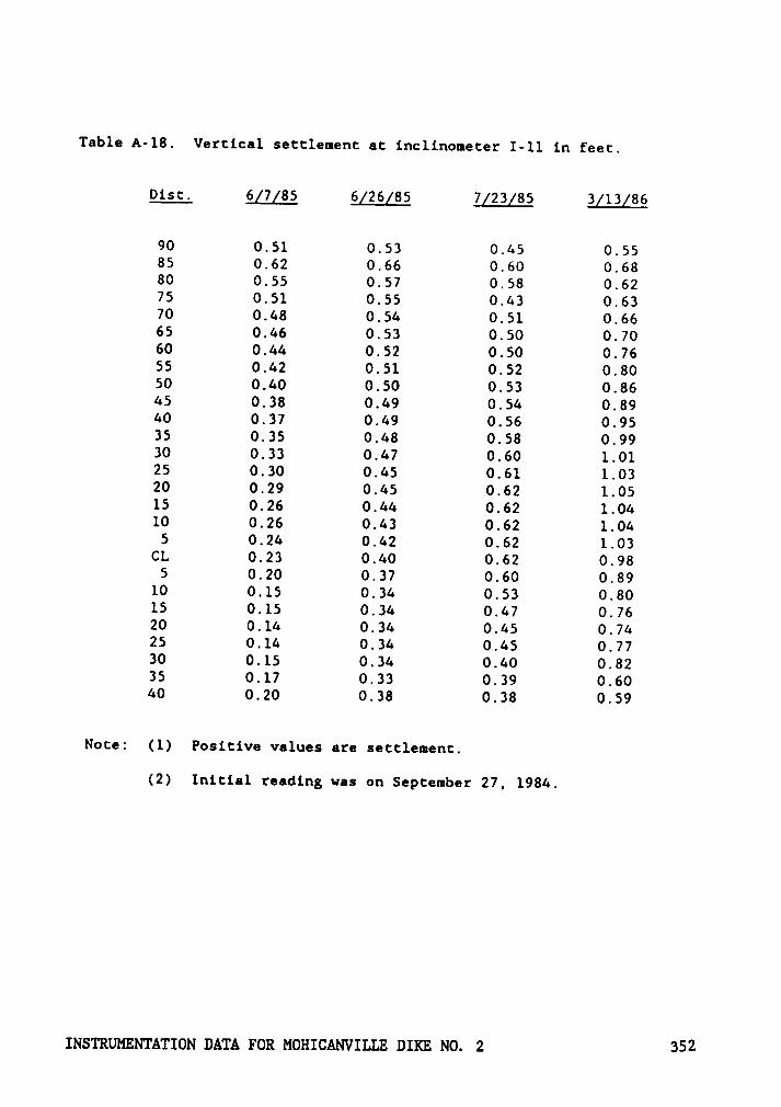
Table A-18. Vertical sectlement ac inclinometer I-11 in feet.
Disc. 6[7[85 6g26g8S 7[23g85 3g13g86
90 0.51 0.53 0.65 0.5585 0.62 0.66 0.60 0.6880 0.55 0.57 0.58 0.6275 0.51 0.55 0.63 0.6370 0.68 0.56 0.51 0.6665 0.66 0.53 0.50 0.7060 0.66 0.52 0.50 0.76S5 0.62 0.51 0.52 0.8050 0.60 0.50 0.53 0.8665 0.38 0.69 0.56 0.8960 0.37 0.69 0.56 0.9535 0.35 0.68 0.58 0.9930 0.33 0.67 0.60 1.0125 0.30 0.65 0.61 1.0320 0.29 0.65 0.62 1.0515 0.26 0.66 0.62 1.0610 0.26 0.63 0.62 1.06
5 0.26 0.62 0.62 1.03CL 0.23 0.60 0.62 0.98
5 0.20 0.37 0.60 0.8910 0.15 0.36 0.53 0.8015 0.15 0.36 0.67 0.7620 0.16 0.36 0.65 0.7625 0.16 0.36 0.65 0.7730 0.15 0.36 0.60 0.8235 0.17 0.33 0.39 0.6060 0.20 0.38 0.38 0.59
Note: (1) Positive values are settlement.
(2) Initial reading was on September 27, 1986.
INSTRUMENTATION DATA FOR MOHICANVILLE DIKE NO. 2 352
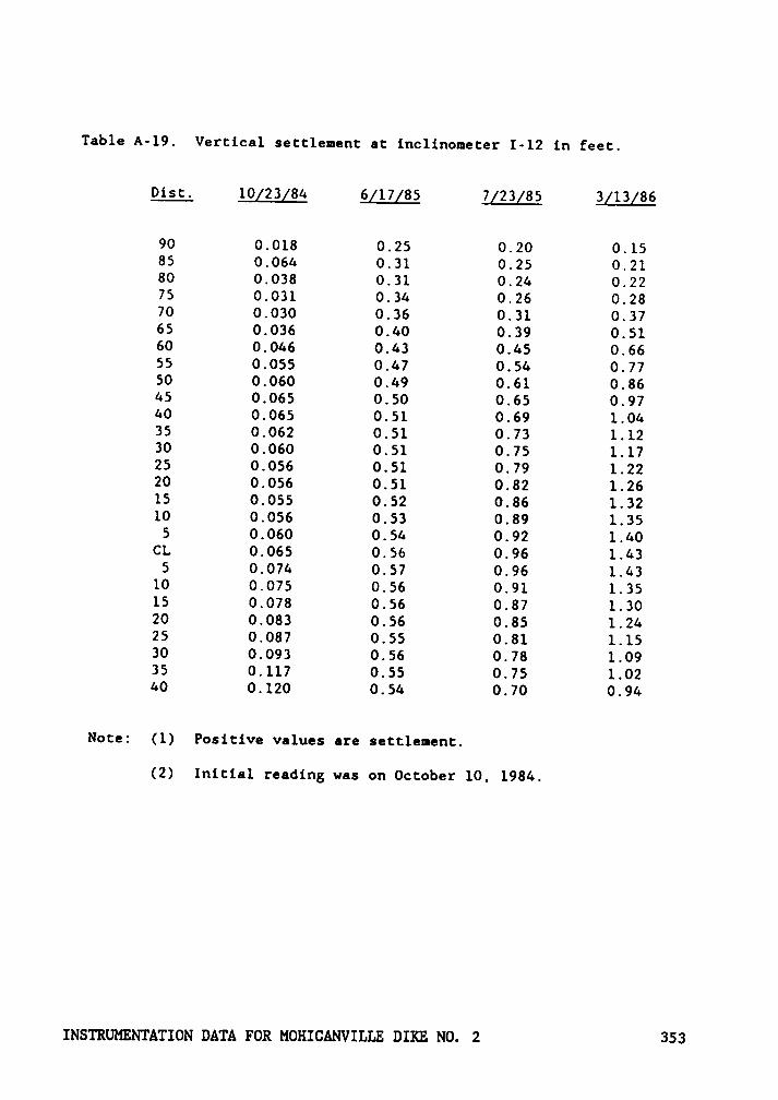
Table A·19. Vertical setclemenc ac inclinomecer I·12 in feet.
Disc. 10g23g86 6g17g85 7g23g85 3g13g86
90 0.018 0.25 0.20 0.1585 0.066 0.31 0.25 0.2180 0.038 0.31 0.26 0.2275 0.031 0.36 0.26 0.2870 0.030 0.36 0.31 0.3765 0.036 0.60 0.39 0.5160 0.066 0.63 0.65 0.6655 0.055 0.67 0.56 0.7750 0.060 0.69 0.61 0.8665 0.065 0.50 0.65 0.9760 0.065 0.51 0.69 1.0635 0.062 0.51 0.73 1.1230 0.060 0.51 0.75 1.1725 0.056 0.51 0.79 1.2220 0.056 0.51 0.82 1.2615 0.055 0.52 0.86 1.3210 0.056 0.53 0.89 1.35
5 0.060 0.56 0.92 1.60CL 0.065 0.56 0.96 1.63
5 0.076 0.57 0.96 1.6310 0.075 0.56 0.91 1.3515 0.078 0.56 0.87 1.3020 0.083 0.56 0.85 1.2625 0.087 0.55 0.81 1.1530 0.093 0.56 0.78 1.0935 0.117 0.55 0.75 1.0260 0.120 0.56 0.70 0.96
Noce: (1) Positive values are sectlement.
(2) Initial reading was on October 10, 1986.
INSTRUMENTATION DATA FOR MOHICANVILLE DIKE NO. 2 353
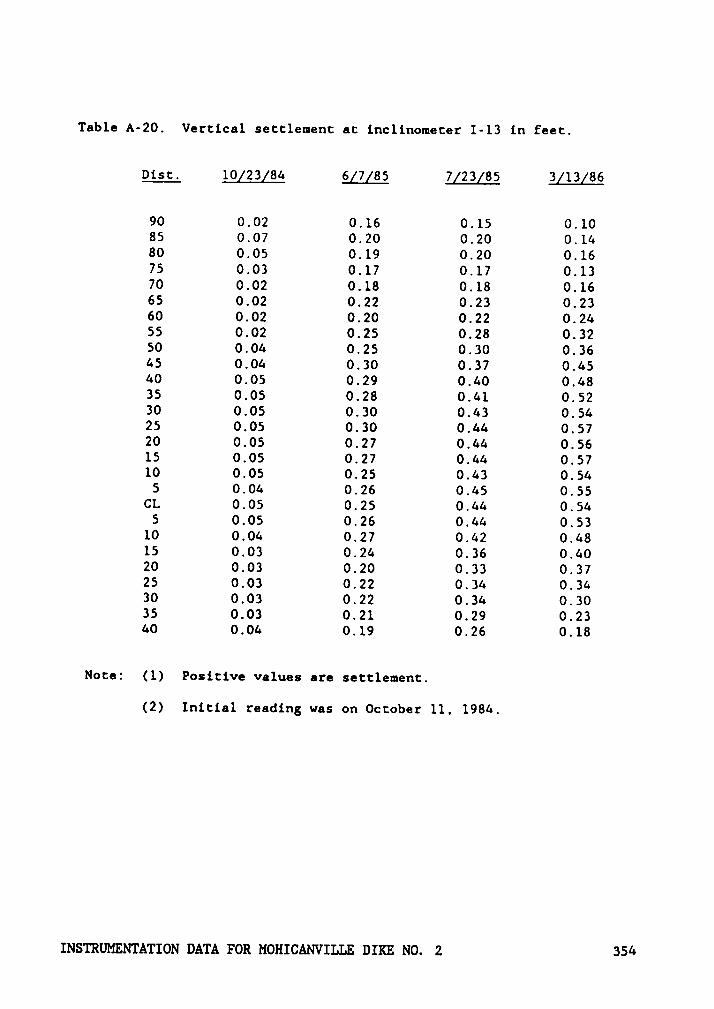
Table A-20. Vertical settlement at inclinometer I-13 in feet.
Disc. 10g23g84 6g7g85 7g23[85 3g13g86
90 0.02 0.16 0.15 0.1085 0.07 0.20 0.20 0.1480 0.05 0.19 0.20 0.1675 0.03 0.17 0.17 0.1370 0.02 0.18 0.18 0.1665 0.02 0.22 0.23 0.2360 0.02 0.20 0.22 0.2455 0.02 0.25 0.28 0.3250 0.04 0.25 0.30 0.3645 0.04 0.30 0.37 0.4540 0.05 0.29 0.40 0.4835 0.05 0.28 0.41 0.5230 0.05 0.30 0.43 0.5425 0.05 0.30 0.44 0.5720 0.05 0.27 0.44 0.5615 0.05 0.27 0.44 0.5710 0.05 0.25 0.43 0.54
5 0.04 0.26 0.45 0.55CL 0.05 0.25 0.44 0.54
5 0.05 0.26 0.44 0.5310 0.04 0.27 0.42 0.4815 0.03 0.24 0.36 0.4020 0.03 0.20 0.33 0.3725 0.03 0.22 0.34 0.3430 0.03 0.22 0.34 0.3035 0.03 0.21 0.29 0.2340 0.04 0.19 0.26 0.18
Note: (1) Positive values are settlement.
(2) Initial reading was on October 11, 1984.
INSTRUMENTATION DATA FOR MOHICANVILLE DIKE NO. 2 354
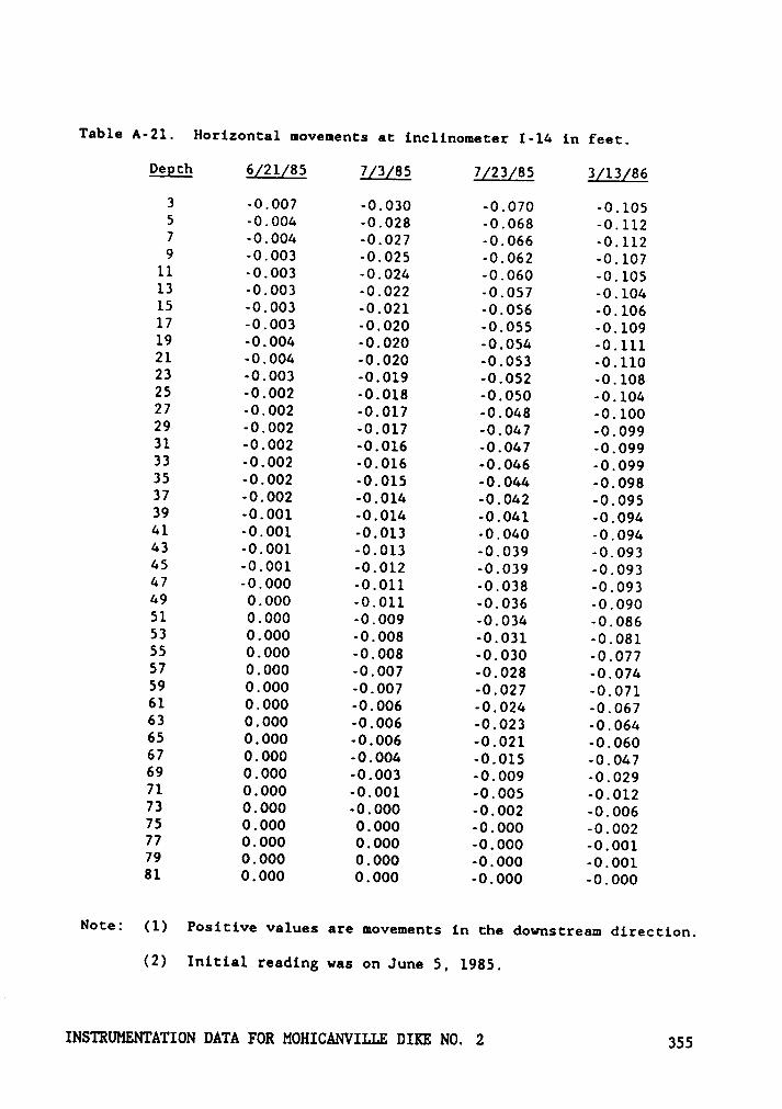
Table A-21. Horizontal movements at inclinometer I-14 in feet.
Degth 6g21g85 7g3g85 7[23g8S 3g13g86
3 -0.007 -0.030 -0.070 -0.1055 -0.004 -0.028 -0.068 -0.1127 -0.004 -0.027 -0.066 -0.1129 -0.003 -0.025 -0.062 -0.107
11 -0.003 -0.024 -0.060 -0.10513 -0.003 -0.022 -0.057 -0.10415 -0.003 -0.021 -0.056 -0.10617 -0.003 -0.020 -0.055 -0.10919 -0.004 -0.020 -0.054 -0.11121 -0.004 -0.020 -0.053 -0.11023 -0.003 -0.019 -0.052 -0.10825 -0.002 -0.018 -0.050 -0.10427 -0.002 -0.017 -0.048 -0.10029 -0.002 -0.017 -0.047 -0.09931 -0.002 -0.016 -0.047 -0.09933 -0.002 -0.016 -0.046 -0.09935 -0.002 -0.015 -0.044 -0.09837 -0.002 -0.014 -0.042 -0.09539 -0.001 -0.014 -0.041 -0.09441 -0.001 -0.013 -0.040 -0.09443 -0.001 -0.013 -0.039 -0.09345 -0.001 -0.012 -0.039 -0.09347 -0.000 -0.011 -0.038 -0.09349 0.000 -0.011 -0.036 -0.09051 0.000 -0.009 -0.034 -0.08653 0.000 -0.008 -0.031 -0.08155 0.000 -0.008 -0.030 -0.077S7 0.000 -0.007 -0.028 -0.07459 0.000 -0.007 -0.027 -0.07161 0.000 -0.006 -0.024 -0.06763 0.000 -0.006 -0.023 -0.06465 0.000 -0.006 -0.021 -0.06067 0.000 -0.004 -0.015 -0.04769 0.000 -0.003 -0.009 -0.02971 0.000 -0.001 -0.005 -0.01273 0.000 -0.000 -0.002 -0.00675 0.000 0.000 -0.000 -0.00277 0.000 0.000 -0.000 -0.00179 0.000 0.000 -0.000 -0.00181 0.000 0.000 -0.000 -0.000
Note: (1) Positive values are movements in the downstream direction.
(2) Initial reading was on June 5, 1985.
INSTRUMENTATION DATA FOR MOHICANVILLE DIKE NO. 2 355
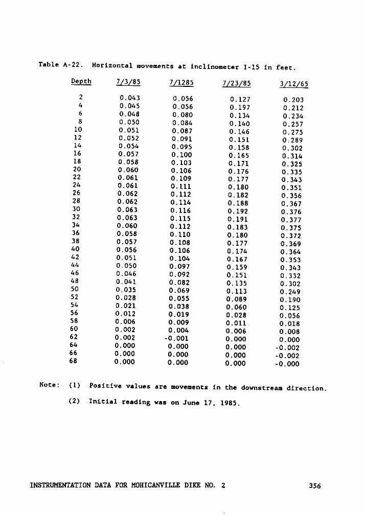
Table A-22. Horizontal movements at inclinometer 1-15 in feet.
Degth 7g3g85 7gl285 7[23g85 3g12g65
2 0.043 0.056 0.127 0.2034 0.045 0.056 0.197 0.2126 0.048 0.080 0.134 0.2348 0.050 0.084 0.140 0.257
10 0.051 0.087 0.146 0.27512 0.052 0.091 0.151 0.28914 0.054 0.095 0.158 0.30216 0.057 0.100 0.165 0.31418 0.058 0.103 0.171 0.32520 0.060 0.106 0.176 0.33522 0.061 0.109 0.177 0.34324 0.061 0.111 0.180 0.35126 0.062 0.112 0.182 0.35628 0.062 0.114 0.188 0.36730 0.063 0.116 0.192 0.37632 0.063 0.115 0.191 0.37734 0.060 0.112 0.183 0.37536 0.058 0.110 0.180 0.37238 0.057 0.108 0.177 0.36940 0.056 0.106 0.174 0.36442 0.051 0.104 0.167 0.35344 0.050 0.097 0.159 0.34346 0.046 0.092 0.151 0.33248 0.041 0.082 0.135 0.30250 0.035 0.069 0.113 0.24952 0.028 0.055 0.089 0.19054 0.021 0.038 0.060 0.12556 ‘
0.012 0.019 0.028 0.05658 0.006 0.009 0.011 0.01860 0.002 0,004 0.006 0.00862 0.002 -0.001 0.000 0.00064 0.000 0.000 0.000 -0.00266 0.000 0.000 0.000 -0.00268 0.000 0.000 0.000 -0.000
Note: (1) Positive values are movements in the downstream direction.
(2) Initial reading was on June 17, 1985.
INSTRUMNTATION DATA FOR MOHICANVILLE DIKE NO. 2 356
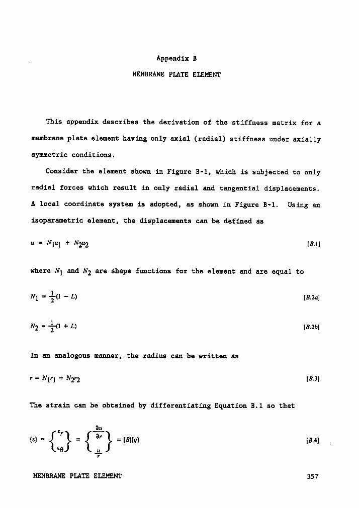
Appendix B
MEMBRANE PLATE ELEMENT
This appendix describes the derivation of the stiffness matrix for a
membrane plate element having only axial (radial) stiffness under axially
symmetric conditions.
Consider the element shown in Figure B-1, which is subjected to only
radial forces which result in only radial and tangential displacements.
A local coordinate system is adopted, as shown in Figure B·1. Using an
isoparametric element, the displacements can be defined as
u = Nlul + N2u2 [B.1]
where N1 and Nj are shape functions for the element and are equal to
L) [1;.2711
N2 = %(1 + L) [B.2b]
In an analogous manner, the radius can be written as
r = Nlrl + N2r2 [B.3]
The strain can be obtained by differentiating Equation B.l so that
Gu‘*BT{=} = = = lBl{q} IB-4l „
697
MEMBRANE PLATE ELEMENT 357
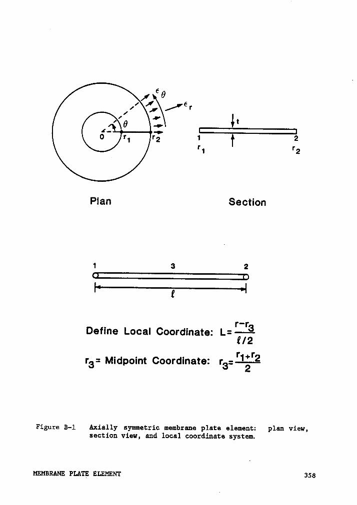
*6/16
I g' I'-r Tt-rF; 1 T 2
r1 1*2
Plan Section
1 3 2
I E I
_ _ I"I'3Define Local Coordmate: L=——
Z!2
- M'd ‘ 1 c d' 1 ·r‘*r2
T3- I DOIII OOT Ina
8.FigureB—l Axially symmetric membrane plate element: plan view,section view, and local coordinate system.
MEMBRANE PLATE ELEMENT 358
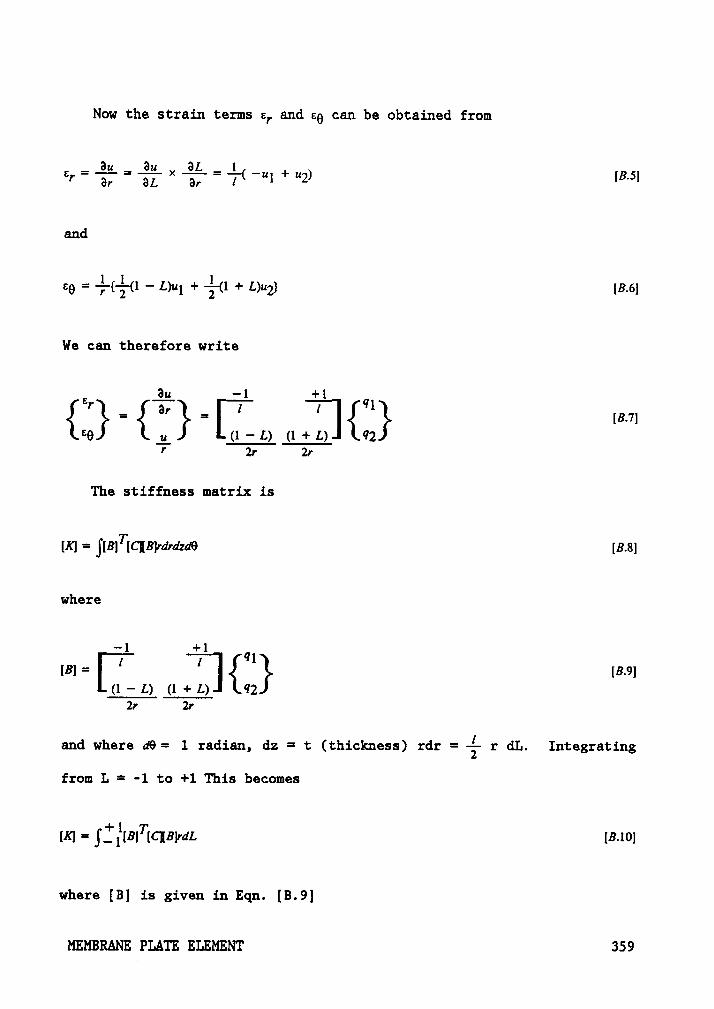
Now the strain terms 6,. and 89 can be obtained from
11151
and
80 = — ml + %(1 + L)u2} [3,6}
We can therefore write
Bu -1 +1B ·— ql{’}={°’}=[’’]{}*9L (1 ·· L) (1 + L) 72
1 26 26
'1'he stiffness matrix is
(K} = j[B]71C][B]rdrdzd6 [6.6}
where
-1 +1_ 1 1 71[6} - 16.9}
(1 — 1.) (1 + L} 7226 2r
and where dl-)= 1 radian, dz = t (thickness) rdr = é r dL. Integrating
from L = -1 to +1 This becomes
1[Kl = IIBITICIBWL IB-101
where [B] is given in Eqn. [B.9]
MEMBRANE PLATE ELEMENT 359
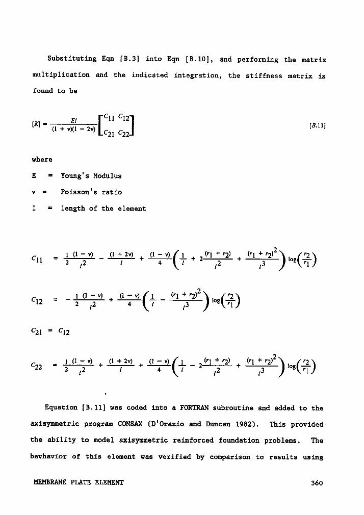
Substituting Eqn [B.3] into Eqn [B.10], and performing the matrix
multiplication and the indicated integration, the stiffness matrix is
found to be
C11 C12161 = II 16-111( + V)( V) C21 C221 1 - 2
where
E = Young's Modulus
v = Poisson°s ratio
l = length of the element
2_ 1 (1 — V) _ (1 + 2V) (1 - V) L (11 + 1;) (11 + 12) V2C11 ”2 I2 1 + 4 (I + 2 I2 +I3C
_ _1<1—V)I
11—V> 1__ (11+1212 I 212 ' 2 I2 4 1 I3 °g 11)
C21 = C12
CI22' 2 I2 1 4 1 I2 I3 °g(11)
Equation [B.11] was coded into a FORTRAN subroutine and added to the
axisymmetric program CONSAX (D'0razio and Duncan 1982). This provided
the ability to model axisymmetric reinforced foundation problems. The
bevhavior of this element was verified by comparison to results using
MEMBRANE PLATE ELEMENT 360
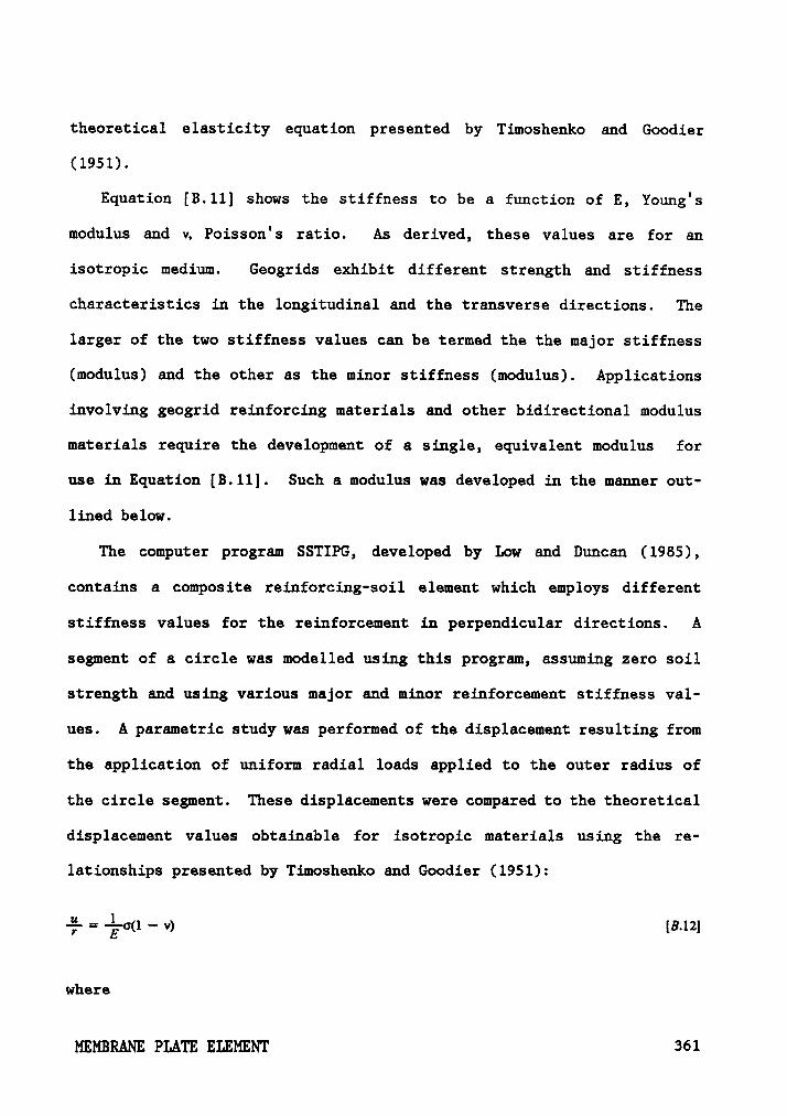
theoretical elasticity equation presented by Timoshenko and Goodier
(1951).
Equation [B.ll] shows the stiffness to be a function of E, Young°s
modulus and w Poisson's ratio. As derived, these values are for an
isotropic medium. Geogrids exhibit different strength and stiffness
characteristics in the longitudinal and the transverse directions. The
larger of the two stiffness values can be termed the the major stiffness
(modulus) and the other as the minor stiffness (modulus). Applications
involving geogrid reinforcing materials and other bidirectional modulus
materials require the development of a single, equivalent modulus for
use in Equation [B.11]. Such a modulus was developed in the manner out-
lined below.
The computer program SSTIPG, developed by Low and Duncan (1985),
contains a composite reinforcing-soil element which employs different
stiffness values for the reinforcement in perpendicular directions. A
segment of a circle was modelled using this program, assuming zero soil
strength and using various major and minor reinforcement stiffness val-
ues. A parametric study was performed of the displacement resulting from
the application of uniform radial loads applied to the outer radius of
the circle segment. These displacements were compared to the theoretical
displacement values obtainable for isotropic materials using the re-
lationships presented by Timoshenko and Goodier (1951):
where
MEMBRANE PLATE ELEMENT 361
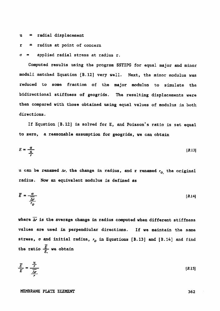
u = radial displacement
r = radius at point of concern
6 = applied radial stress at radius r.
Computed results using the program SSTIPG for equal major and minor
moduli matched Equation [B.12] very well. Next, the minor modulus was
reduced to some fraction of the major modulus to simulate the
bidirectional stiffness of geogrids. The resulting displacements were
then compared with those obtained using equal values of modulus in both
directions.
If Equation [B.12] is solved for E, and Poisson's ratio is set equal
to zero, a reasonable assumption for geogrids, we can obtain
E = % [B.13]
u can be renamed An the change in radius, and r renamed QL the original
radius. Now an equivalent modulus is defined as
E =é
[B.l4]’o
where Ä; is the average change in radius computed when different stiffness
values are used in perpendiular directions. If we maintain the same
stress, 6 and initial radius, ro in Equations [B.l3] and [B.14] and find
the ratio % we obtain
= -1%- [8.15]
MEMBRANE PLATE ELEMENT 362

Values of Ä; were determined by performing a parametric study using
SSTIPG in which values of the minor modulus were taken as some fraction
of the major modulus. From this study, the curve in Figure B.2 was de-
veloped, in which the equivalent modulus divided by the major modulus is
shown to be a function of the ratio of the minor and major moduli. This
curve was found to be independent of the major modulus value and is ap-
plicable to any bidirectional stiffness material with Poisson's ratio
equal to zero.
MEMBRANE PLATE ELEMENT 363
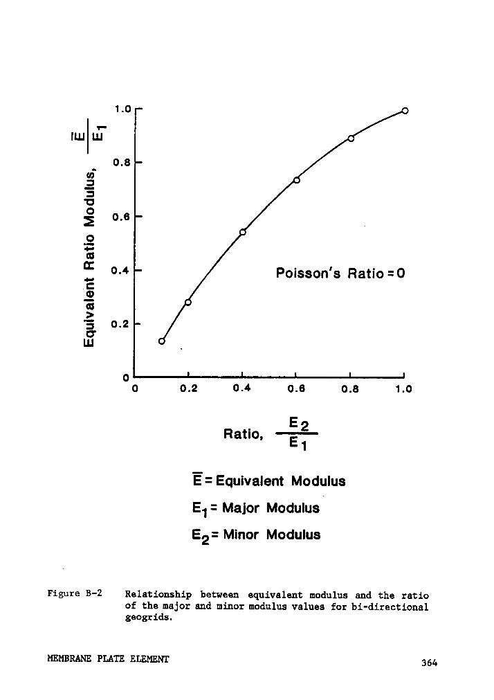
1.0
7*
ILIJ LIJ
0.80)23'¤§ 0.6 1.2dl!
E__ °·‘Poisson's Ratio=0
.C2¤>'5 0.2UUJ .
00 0.2 0.4 0.6 0.8 1.0
E 2Ratio, ·—····E1
E: Equivalent Modulus
E1: Major Modulus
E2: Minor Modulus
. Figure B-Z Relationship between equivalent modulus and the ratioof the major and minor modulus values for bi-directionalgeogrids.
MEMBRANE PLATE ELEMENT ggg
Appendix C
USER'S GUIDE FOR PROGRAM CON2D86
C.1 Introduction
The program CON2D86 is a plane strain finite element computer program
for analysis of stresses, displacements and consolidation in saturated
and partly saturated earth masses. The program can be used to analyze
consolidation in embankment dams during and after construction, and in
foundation soils subject to surface loads imposed by fills, buildings and
storage tanks. The program treats the coupled problem of deformation and
fluid flow, and can be used to calculate movements and pore pressures
under undrained, partly drained and fully drained conditions. Reinforced
soil structures can be analyzed using bar elements.
CON2D86 was originally developed by Chang and Duncan (1977) and was
later modified by Duncan et al. (1981). The program follows the general
programming concepts and solution techniques developed by Wilson (1970)
and Bathe and Wilson (1976). The present version incorporates a bar el-
ement to model reinforcement, and provides enhanced source code documen-
tation and efficiency.
USER°S GUIDE FOR PROGRAM CON2D86 365

C.2 Program Operation
C.2.l Systems and Sign Convention
The global coordinate system is a right handed X-Y system with X in-
creasing to the right and Y increasing vertically.
Soil element and interface normal stresses are positive in compression
and negative in tension. The soil stresses are all effective stresses.
Positive pore pressures are compressive. Total stresses are obtained by
adding pore pressures at the center of elements to the effective soil
stresses.
Bar element forces are output in a local coordinate system. Axial
force is positive if the member is in compression and negative if in
tension.
C.2.2 Storage Allocation
Dynamic storage allocation (Bathe and Wilson 1976) is used within the
program and storage is allocated at the time of execution. The storage
can be readily adjusted through the COMMON (A) statement in the source
code. Storage requirements are checked immediately after reading the
control data, and if insufficient, an error message printed detailing the
minimum storage requirements for the problem and execution is halted.
The equation-solving subroutines use only one-half of the full banded
stiffness matrix. Secondary storage (disk or tape storage) is used to
USER'S GUIDE FOR PROGRAM CON2D86 366
minimize the amount of core storage required by solving the equations by
blocks (Wilson et al. 1974). The smaller the number of equations per
block, the greater is the required number of transfers between core and
secondary storage, and the more costly is the solution procedure. Thus,
the more storage allocation exceeds the minimum value, the larger is the
number of equations per block, and hence the shorter is the solution time.
0.2.3 Element Types
CON2D86 has three types of elements as follows:
1. Soil elements are four-to-eight variable node, two·dimensional,
isoparametric elements as described by Bathe and Wilson (1976). Each
node may also have a pore pressure degree-of-freedom. Any number of
nodes from four to eight can be specified for each element. Trian-
gular shaped elements can be formed by superimposing nodes. The nodal
point numbers must be specified in the order I, II, III, IV, V, VI,
VII, VIII as shown in the upper part of Figure C-1. For an element
with fewer than eight nodes, the nodal point numbers of the omitted
nodes are set equal to zero, as shown in the bottom of Figure C-1.
For triangular elements, the nodal point number III must be equal to
the nodal point number IV.
2. Bar elements are two node elements with axial stiffness only (no
flexural or shear resistance), and may be used to connect any two
nodal points.
USER'S GUIDE FOR PROGRAM CON2D86 367
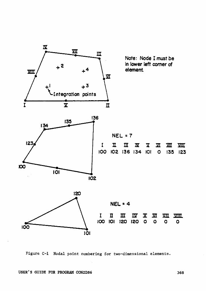
II E III _ Note: Node Imust be2 in lower left comer of"’ +4 element
H+‘ +3\-Integration points
I I II
l36I35
l54
NEL = 7*23 1 Il III 11 1 EI III 1111
IOO IOZ I36 I34 IOI O l35 I23
IOO_ IOI
IO2
IE
NEL=4
I II III DT I II IH. IIII.IOOIOIIEIZOO O O 0
IOO .IOI
Figure C—l Nodal point numbering for l:wo—d:i.mensional elements.
UsER's GUIDE EUR PROGRAM coN2D66 368
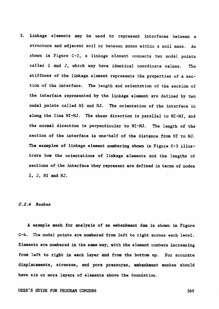
3. Linkage elements may be used to represent interfaces between a
structure and adjacent soil or between zones within a soil mass. As
shown in Figure C-2, a linkage element connects two nodal points
called I and J, which may have identical coordinate values. The
stiffness of the linkage element represents the properties of a sec-
tion of the interface. The length and orientation of the section of
the interface represented by the linkage element are defined by two
nodal points called NI and NJ. The orientation of the interface in
along the line NI-NJ. The shear direction is parallel to NI-NJ, and
the normal direction is perpendicular to NI-NJ. The length of the
section of the interface is one-half of the distance from NI to NJ.
The examples of linkage element numbering shown in Figure C-3 illus-
trate how the orientations of linkage elements and the lengths of
sections of the interface they represent are defined in terms of nodes
I, J, NI and NJ. h
6.2.4 Hesbes
A example mesh for analysis of an embankment dam is shown in Figure
C-4. The nodal points are numbered from left to right across each level.
Elements are numbered in the same way, with the element numbers increasing
from left to right in each layer and from the bottom up. For accurate
displacements, stresses, and pore pressures, embankment meshes should
have six or more layers of elements above the foundation.
USER°S GUIDE FOR PROGRAM CON2D86 369
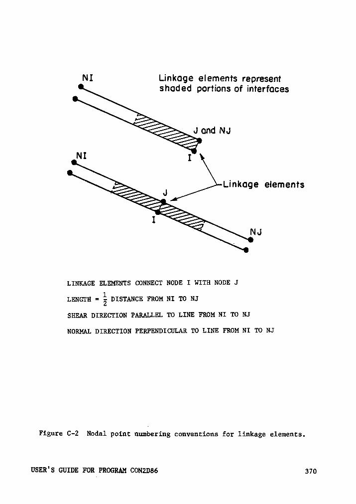
NI Linkoge elements representshoded portlons of interfoces
J ond NJ
NI 1
Linkoge elements~ J
INJ
LINKAGE ELEMENTS CONNECT NODE I WITH NODE J
LENGTH = ä DISTANCE FROM NI TO NJ
SHEAR DIRECTION PARALLEL TO LINE FROM NI TO NJ
NORMAL DIRECTION PERPENDICULAR TO LINE FROM NI TO NJ
Figure C-2 Nodal poiut numberiug conveutions for liukage elements.
USER'S GUIDE FOR PROGRAM CON2D86 370

La er n+I162 y
I3!
@ I22I2!
!!2Layer n
!!!
IO2
· IO!
LinkageElement Q Q El EQ
1 101 102 112 102
2I
111 112 122 102
3 121 122 122 112
4 121 122 132 122
Linkage element C) represents half of interfacefrom node 112 to node 122, and would be added tomesh with layer n. Linkage element GD representshalf of interface from node 122 to node 132, andwould be added to mesh with layer n + 1.
Nodes 101 and 102, lll and 112, etc., may havesame coordinates.
Figure C—3 Linkage element example.
USER'S GUIDE FOR PROGRAM CONZDB6 371
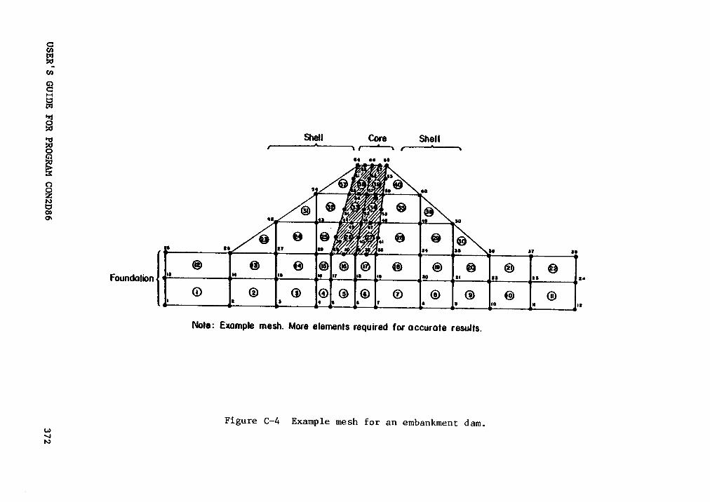
®@@O6
éE
3a
,§
,_,C20
Q)
=®
®6
°§E
®®
6E
E8
szQ
SZ
§M£“&>,&Ü;§\;,~-5
¤~
E‘
©-
,ä
YQEM@„
;ä
E·
“·®·
%6;
*E
0
®®
@g
E
=••
2¤•
äQ
)2E
!E
-•§D
:3
¤=~2
2
M€2SEB
USER'SGUIDE
FORPROGRAM
CON2D86372
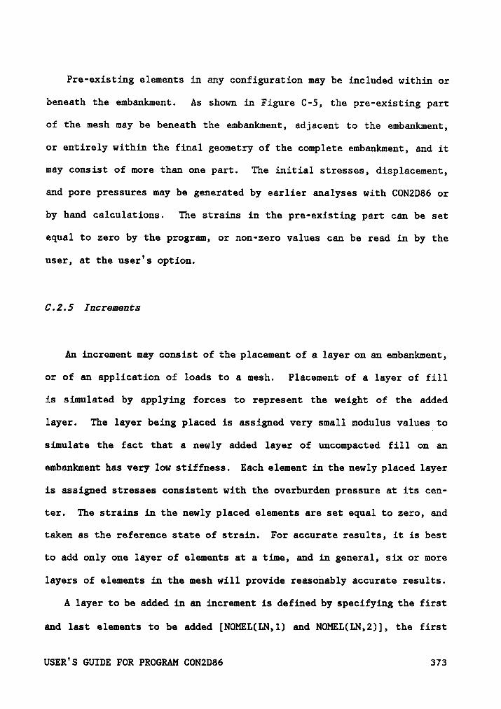
Pre·existing elements in any configuration may be included within or
beneath the embankment. As shown in Figure C-5, the pre·existing part
of the mesh may be beneath the embankment, adjacent to the embankment,
or entirely within the final geometry of the complete embankment, and it
may consist of more than one part. The initial stresses, displacement,
and pore pressures may be generated by earlier analyses with CON2D86 or
by hand calculations. The strains in the pre-existing part can be set
equal to zero by the program, or non-zero values can be read in by the
user, at the user's option.
0.2.5 Iucrenants
An increment may consist of the placement of a layer on an embankment,
or of an application of loads to a mesh. Placement of a layer of fill
is simulated by applying forces to represent the weight of the added
layer. The layer being placed is assigned very small modulus values to
simulate the fact that a newly added layer of uncompacted fill on an
embankment has very low stiffness. Each element in the newly placed layer
is assigned stresses consistent with the overburden pressure at its cen-
ter. The strains in the newly placed elements are set equal to zero, and
taken as the reference state of strain. For accurate results, it is best
to add only one layer of elements at a time, and in general, six or more
layers of elements in the mesh will provide reasonably accurate results.
A layer to be added in an increment is defined by specifying the first
and last elements to be added [NOMEL(LN,1) and NOMEL(LN,2)], the first
USER'S GUIDE FOR PROGRAM CON2D86 373
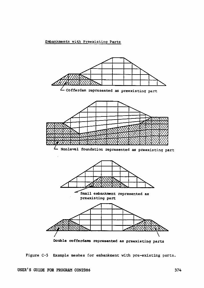
Embankments with Preexisting Parts
4-;L----
,4-----;,6%%------;Cofferdam represented as preexisting part
A---.
^‘===!=..4ä=---=?I0HIh7 { ißlllnllIIIIIIIIIIIIIIIIIII -||I5Zß??B;Zü2?!!2
I { . Q I E'
Nonlevel foundation represented as preexisting part
4-;4---;
4----;4--%%%--;
Small embankment represented as”preexisting part
l--
Aé===ä„.Dauble cofferdams represented as preexistinq parts
Figure C—5 Example meshes for embankment with pre—exisci¤g parts.
USER°S GUIDE FOR PROGRAM CON2D86 374
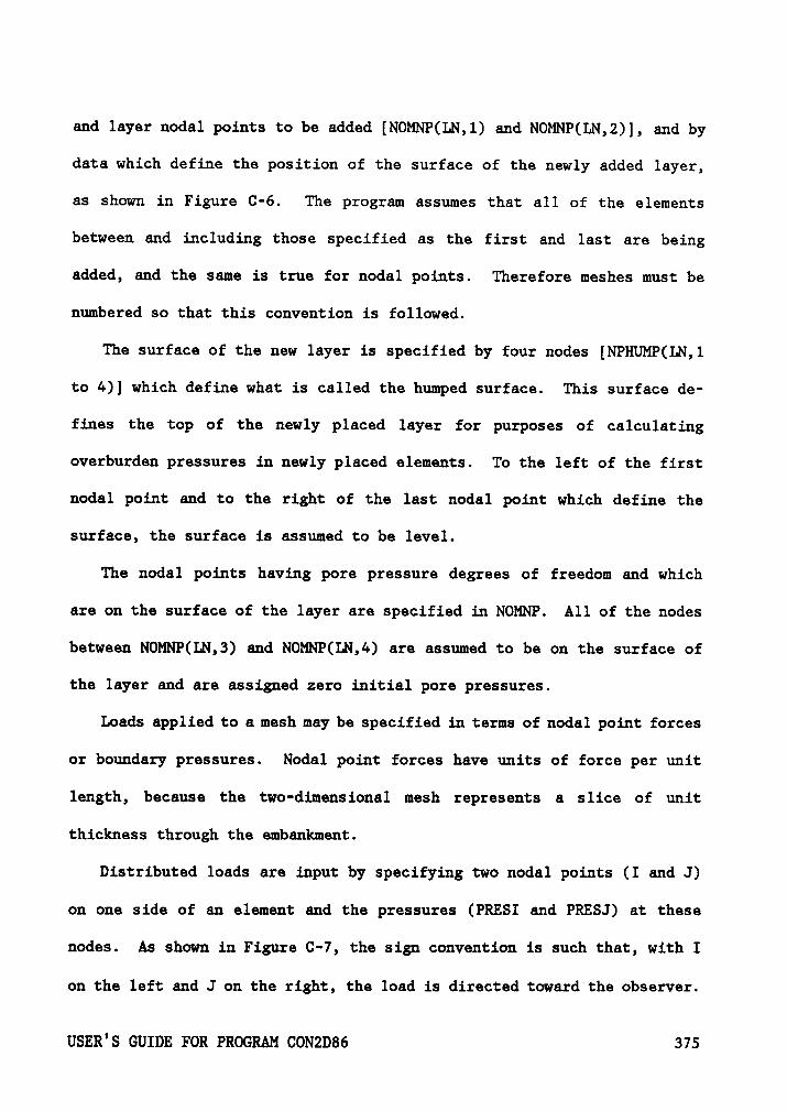
and layer nodal points to be added [NOMNP(LN,1) and NOMNP(LN,2)], and by
data which define the position of the surface of the newly added layer,
as shown in Figure C-6. The program assumes that all of the elements
between and including those specified as the first and last are being
added, and the same is true for nodal points. Therefore meshes must be
numbered so that this convention is followed.
The surface of the new layer is specified by four nodes [NPHUMP(LN,1
to 4)] which define what is called the humped surface. This surface de-
fines the top of the newly placed layer for purposes of calculating
overburden pressures in newly placed elements. To the left of the first
nodal point and to the right of the last nodal point which define the
surface, the surface is assumed to be level.
The nodal points having pore pressure degrees of freedom and which
are on the surface of the layer are specified in NOMNP. All of the nodes
between NOMP(LN,3) and NOMNP(LN,4) are assumed to be on the surface of
the layer and are assigned zero initial pore pressures.
Loads applied to a mesh may be specified in terms of nodal point forces
or boundary pressures. Nodal point forces have units of force per unit
length, because the two-dimensional mesh represents a slice of unit
thickness through the embankment.
Distributed loads are input by specifying two nodal points (I and J)
on one side of an element and the pressures (PRESI and PRESJ) at these
nodes. As shown in Figure C-7, the sign convention is such that, with I
on the left and J on the right, the load is directed toward the observer.
USER°S GUIDE FOR PROGRAM CON2D86 375
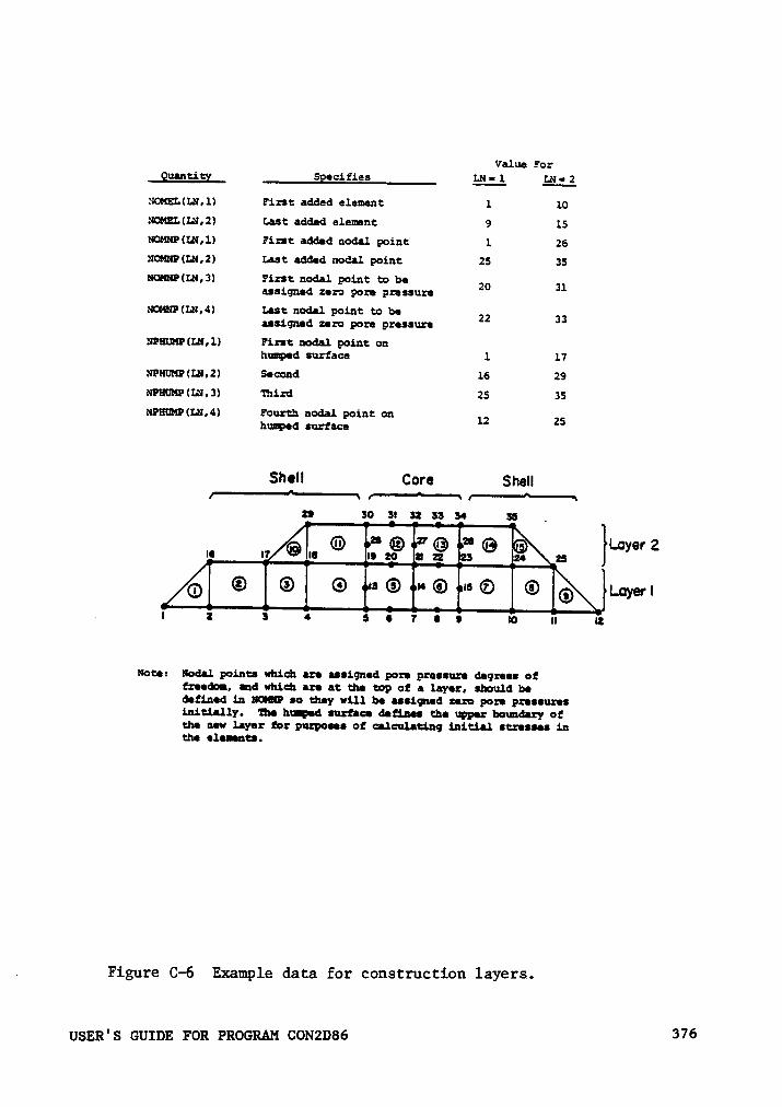
Value ForQuantig soecifies LN- 1 LN- 2
NOME!•(LN,l) First added element 1 10NOMEMLN,2) Last added element 9 15N¤MNP(IJl,l) First added nodal point 1 26NOMNP(LN,2) Bst added nodal point 25 35NOHNHIN,3) First nodal point to be 20 31assiqned zero pcre pressure
NOMNHIN,4) Bst nodal point to be 22 33assigned zero pore pressureNPHlJMP(LN,l) First nodal point on
humped surface 1 17
NPllUH!(LN„2l Second 16 29NPHUMP(IN„3) Third 25 35NPHUMMLN,4) Fourtn nodal point on 12 25huaped surface
Shell Core Shell
29 S0 Sl 32 33 54 35 _
G ® · ® ' @ ¤ @ IQ Loyer 2II I7 II II zu 2 22 23 25
ABE @ @ ·—«»«·I 2 5 4 5 e 7 s s IO II I2
Note: Nodal points which are assiqned pore pressure deqrees offreeärn, and whldx are at the top of a layer, should bedefined in IGN! so they will be assigned zero pore pressureslnltially. The hzqed surface deflnes the wper boundary ofthe new layer for purposes of calculatinq initial stresses inthe elennts.
, Figure C-6 Example data for construction layers.
USER'S GUIDE FOR PROGRAM CON2D86 376
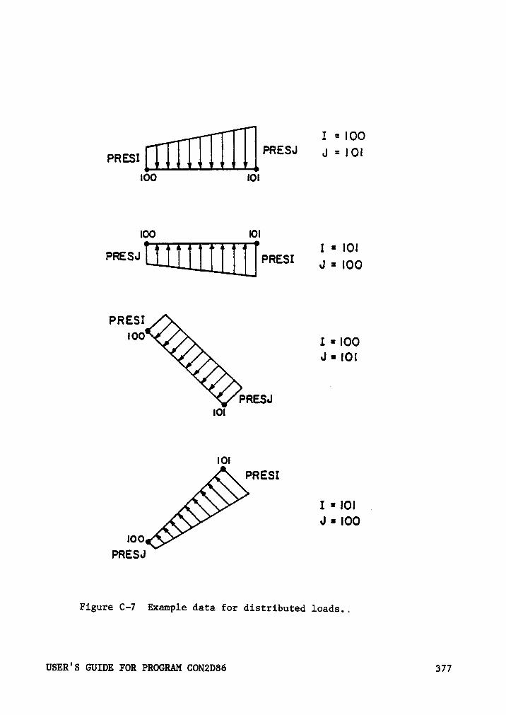
I = IOOPRESJ =Passr " '°'
100 I01
l00 IOII = IOIPRESJ Pass: J = JOO
PRESI
'°° x = 100J = IOI
PRESJ101
IOIPRESI
I = IOI „J = IOO
I00PRESJ
Figure C-7 Example data for distributed loads..
USER'S GUIDE FOR PROGRAM CON2D86 377

The data required to describe changes in the reservoir level on the
upstream side of a dam are illustrated in Figure C·8. Within the shell,
elements are subjected to a reduction in effective unit weight when they
are submerged below a rising reservoir, and an increase in effective unit
weight when they emerge above a falling reservoir.
The changes in water pressure along the shell/core boundary are cal-
culated within the program using the information specified in NUMSWP(I),
LEVOLD and NEWLEV. Because these data are specified in terms of nodal
point numbers, each water level elevation must coincide with the elevation
of a nodal point on the shell/core boundary. Because of the sign con-
vention used in the program, downstream must be in the positive x-
direction (to the right).
0.3 Program Organization
The main program (CON2D86) reads and prints the control data and
monitors all operations by calling the subroutines in the specified order.
1. Subroutine LAYOUT controls the subroutines which read the input data.
Subroutine LAYOUT calls INPTNP to read and print nodal point data,
MATIN to read and print soil material property data, BARIN to read
and print bar element data, LINKIN to read and print linkage element
data, PREXIN to read and print pre-existing element data, ELEMIN to
read and print soil element data, and CLBAND to calculate the band-
width for the problem. Storage requirements are calculated and if
USER'S GUIDE FOR PROGRAM CON2D86 378
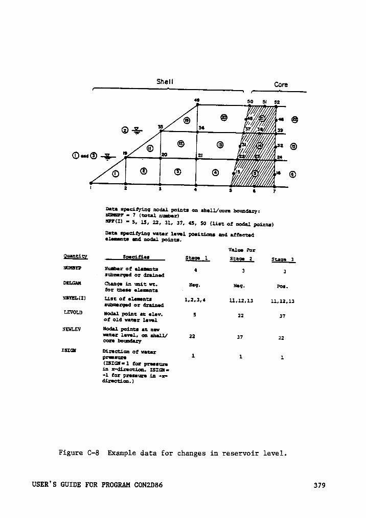
SUB'! Cqrg4• so sn sz
7 l@ @.1/ es @Q .1
’°*° *7 Ä =•
®••«@ ..;.. " =°ß
=•
ABHHW)n 2 3 4 s •7
Data specityinq nodal points on shell/core boundery:mm! - 1 (total nuuber)NPNI) • S, 1.5, 22, 31, 37, 45, S0 (list ot ¤oda..'L points)Data specityinq vater level poeitions md etfectedelements end nodal poinu.
Value ForQuentig Soecifies Staa 1 Steg 2 Stage 3
NUHIYP Huber ot eluents 4 3 3Submerqed or dreinedDELGAM Qzanqe in mit vt. Neg. Neg. Pos.tor these elnunts ·NIY!L(I) ue: ot •1.•¤•¤¤ 1,2,3,4 11,12,13 1.1,12,1:submezqed or drsinedLzvow uodu. pour az elev. s 22 37ot old unter level
NEW;}-gv Nodal points at newwater level, on shell! 22 37 22core bouzduy
ISIGI Direction ot vater 1 1 1!$l¤!I
tor pressurein x·d.L:ectio¤. ISI¤•·l tor pressure Ln •x—direction.)
Figure C-8 Example data for changes in reservoir level.
USER°S GUIDE FOR PROGRAM CON2D86 379

the problem requires more storage, a message is printed and execution
halted.
2. Subroutine INITL reads and/or calculates the initial values of
stresses, strains, displacements and pore pressures for pre-existing
elements and added layer elements.
3. Subroutine FORMB establishes the strain-displacement matrix for the
soil elements by calling BMATPS, which forms the strain-displacement
matrix for a four- to eight-node isoparametric, quadrilateral ele-
ment. BMATPS calls JACOBI to form the Jacobian, which calls SHAPE
to calculate the shape functions.
4. Subroutine CALBLK reads the control data for each increment and de-
termines the number of elements and nodal points being analyzed, the
number of elements and nodal points in the pre-existing part and added
layers, the number of equations, the number of equations in each
block, and the number of blocks for each increment.
5. Subroutine FVECT calculates nodal point forces due to weights of added
elements, or due to buoyancy forces and reads and prints concentrated
load data and boundary pressure data.
6. Subroutine ELSTFF formulates the stiffness matrix for each element.
ELSTFF call STST to form the stress-strain relationship for the soil
elements and calls MODIFY to modify the load vector for each time
USER'S GUIDE FOR PROGRAM CON2D86 380
step. STST calls POICAL and LAMCAL to compute the current values of
Poisson°s ratio and lambda, calls ELAST to calculate the elastic part
of the stress-strain relationship, and calls CAMCLY to calculate the
elasto-plastic stress-strain relationship. ELSTFF calls QK to cal-
culate the current compressibility and permeability of the pore fluid
in each element.
7. Subroutine ADDSTF forms the global stiffness matrix. The soil element
stiffness values are read from tape and the stiffness values for bar
and linkage elements are found by calling BRSTIF and LKSTIF.
8. Subroutine TRIAFAC triangulizes the global stiffness matrix.
9. Subroutine REDVK back substitutes and solves the equations for dis-
placement and pore pressure.
10. Subroutine RESULT calculates the current values of stress and strain.
RESULT calls OUTPUT to print out the results.
0.4 Data Input Guide
0.4.1 Control Data
0.4.1.1 Heading Data (72A)
HEAD Title for program identification.
0.4.1.2 First Control Data Data
NUMELT Total number of soil elements in the complete mesh.
NUHNPT Total number of nodal points in the complete mesh.
NUHMAT Number of different soil material types.
USER'S GUIDE FOR PROGRAM CON2D86 381
NUMCEL Number of soil elements in the pre-existing part.
NUNCNP Number of nodal points in the pre-existing part.
NLAY Number of construction layer increments.
NFORCE Number of load increments after construction.
NUMSWP Total number of nodal points on the shell/core boundary atwhich changes in water pressure will occur during any ofthe steps of the analysis.
0.4.1.3 Second 0ontro1 Data Data
NBRELT Total number of bar elements in the complete mesh.
NRMAT Number of different bar material types.
NUMCBR Number of bar elements in the pre-existing part.
NLKELT Total number of linkage elements in the complete mesh.
NLKHAT Number of different linkage material types.
NUMCLK Number of linkage elements in the pre-existing part.
0.4.2 Nodal point and boundary condition data.
N Nodal point number.
X(Nl X-coordinate (+ to the right).
Y(Nl Y·coordinate (+ up).
ID(N,1) Boundary condition code for displacement in the x-direction.
ID(N,2) Boundary condition code for displacement in the y-direction.
ID(N,3) Boundary condition code for pore pressure.
Nodal points must be read in sequence. If nodal point data areomitted, the coordinates of a series of nodal points are generatedautomatically at equal spacing between those specified. The boundarycondition codes for the generated nodal points are set equal to theboundary condition codes for the previous nodal point. The first andlast points must be specified.
The boundary condition code convention is as follows:
miantitxßnuditigaßnde
USER°S GUIDE FOR PROGRAM CON2D86 382
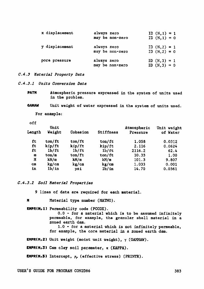
x displacement always zero ID (N,1) = 1may be non-zero ID (N,1) = 0
y displacement always zero ID (N,2) = 1may be non-zero ID (N,2) = 0
pore pressure always zero ID (N,3) = 1may be non-zero ID (N,3) = 0
0.4.3 Material Property Data
0.4.3.1 Units Gonversion Data
PATH Atmospheric pressure expressed in the system of units usedin the problem.
GAHAW Unit weight of water expressed in the system of units used.
For example:
offUnit Atmospheric Unit weight
Length Weight Cohesion Stiffness Pressure of Water
ft ton/ft ton/ft ton/ft 1.058 0.0312ft kip/ft kip/ft kip/ft 2.116 0.0624ft lb/ft lb/ft lb/ft 2116.2 62.4
m ton/m ton/ft ton/ft 10.33 1.00M kN/m kN/m kN/m 101.3 9.807
cm kg/cm kg/cm kg/cm 1.033 0.001in lb/in psi lb/in 14.70 0.0361
0.4.3.2 Soil Material Properties
9 lines of data are required for each material.
H Material type number (MATNO).
EHPR(H•1) Permeability code (PCODE).0.0 - for a material which is to be assumed infinitely
permeable, for example, the granular shell material in azoned earth dam.
1.0 - for a material which is not infinitely permeable,for example, the core material in a zoned earth dam.
EHPR(H,2) Unit weight (moist unit weight), y (GAMMAW).
EHPR(H•3) Cam clay soil parameter, x (KAPPA).
EHPR(H•5) Intercept, pr (effective stress) (PRINTR).
USER°S GUIDE FOR PROGRAM CON2D86 383
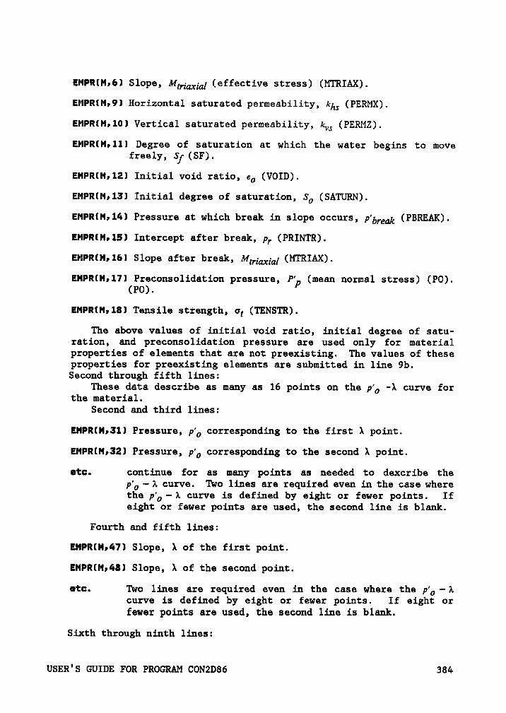
EMPR(M,6) Slope, bqnmxüd (effective stress) (MTRIAX).
EMPR(Mp9l Horizontal saturated permeability, kh,(PERMK).
EMPR(M,10) Vertical saturated permeability, bu (PERMZ).
EMPR(M;11) Degree of saturation at which the water begins to movefreely, ST (SF).
EMPR(M,12) Initial void ratio, eb (VOID).
EMPR(M,13) Initial degree of saturation, Sb (SATURN).
EMPR(M,14) Pressure at which break in slope occurs, pb„bak (PBREAK).
EMPR(M,15) Intercept after break, pr (PRINTR).
EMPR(M,16) Slope after break, bqÜwdb](MTRIAX).
EMPR(M•17) Preconsolidation pressure, Pb (mean normal stress) (PO).(PO).
EMPR(M•18) Tensile strength, 6t(TENSTR).
The above values of initial void ratio, initial degree of satu-ration, and preconsolidation pressure are used only for materialproperties of elements that are not preexisting. The values of theseproperties for preexisting elements are submitted in line 9b.Second through fifth lines:
These data describe as many as 16 points on the pb -X curve forthe material.
Second and third lines:
EMPR(H,31) Pressure, pb corresponding to the first X point.
EMPR(M,32) Pressure, pb corresponding to the second X point.
etc. continue for as many points as needed to. dexcribe thepb)-A curve. Two lines are required even in the case wherethe pb-1 curve is defined by eight or fewer points. Ifeight or fewer points are used, the second line is blank.
Fourth and fifth lines:
EMPR(H»47) Slope, X of the first point.
EMPR(M•48l Slope, X of the second point.
etc. Two lines are required even in the case where the pb-Icurve is defined by eight or fewer points. If eight orfewer points are used, the second line is blank.
Sixth through ninth lines:
USER'S GUIDE FOR PROGRAM CON2D86 384
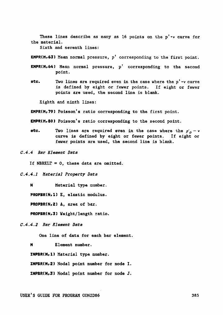
These lines describe as many as 16 points on the p'-v curve forthe material.
Sixth and seventh lines:
EMPR(M,63) Mean normal pressure, p' corresponding to the first point.
EMPR(M•64) Mean normal pressure, p' corresponding to the secondpoint.
etc. Two lines are required even in the case where the p'-v curveis defined by eight or fewer points. If eight or fewerpoints are used, the second line is blank.
Eighth and ninth lines:
EMPR(H,79l Poisson°s ratio corresponding to the first point.
ENPR(M,80) Poisson°s ratio corresponding to the second point.
etc. Two lines are required even in the case where the pb·-vcurve is defined by eight or fewer points. If eight orfewer points are used, the second line is blank.
0.4.4 Bar Element Data
If NBRELT = 0, these data are omitted.
0.4.4.1 Material Property Data
N Material type number.
PROPBR(N,1) E, elastic modulus.
PROPBR(N,Z) A, area of bar.
PROPBR(N»3l Weight/length ratio.
0.4.4.2 Bar Element Data
One line of data for each bar element.
M Element number.
INPBR(M,1) Material type number.
INPBR(M,2) Nodal point number for node I.
INPBR(N,3) Nodal point number for node J.
USER°S GUIDE FOR PROGRAM CON2D86 385
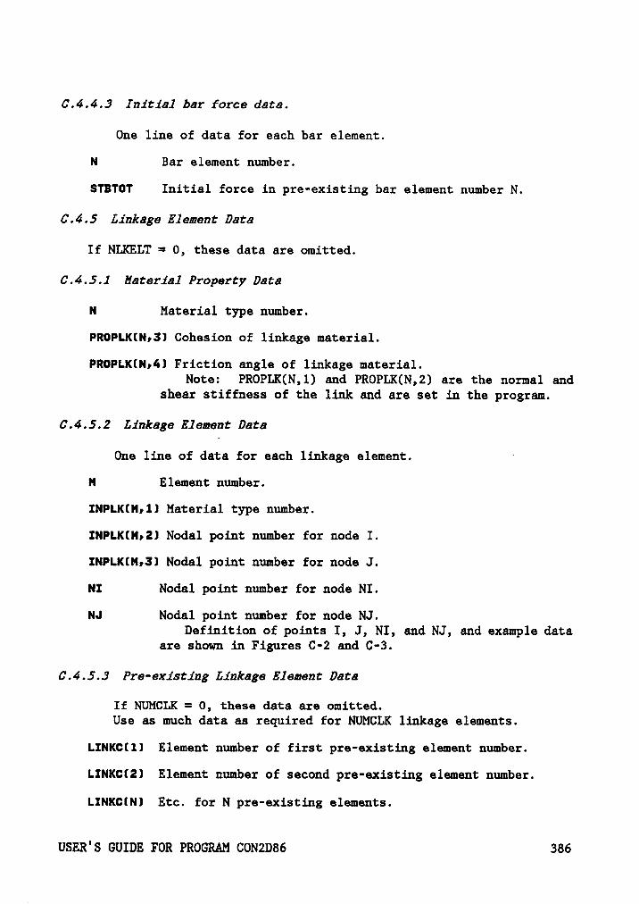
0.4.4.3 Initial bar force data.
One line of data for each bar element.
N Bar element number.
STBTOT Initial force in pre·existing bar element number N.
0.4.5 Linkage Element Data
If NLKELT = O, these data are omitted.
0.4.5.1 Material Property Data
N Material type number.
PROPLK(N,3) Cohesion of linkage material.
PROPLK(N•4) Friction angle of linkage material.Note: PROPLK(N,1) and PROPLK(N,2) are the normal and
shear stiffness of the link and are set in the program.
0.4.5.2 Linkage Element Data
One line of data for each linkage element. ·
N Element number.
INPLK(N,1) Material type number.
INPLK(M,2) Nodal point number for node I.
INPLK(N•3l Nodal point number for node J.
NI Nodal point number for node NI.
NJ Nodal point number for node NJ.Definition of points I, J, NI, and NJ, end example data
are shown in Figures C·2 and C-3.
0.4.5.3 Pre-existing Linkage Element Data
If NUMCLK = 0, these data are omitted.Use as much data as required for NUMCLK linkage elements.
LINKC(1) Element number of first pre-existing element number.
LINKC(2l Element number of second pre-existing element number.
LINKCINI Etc. for N pre-existing elements.
USER°S GUIDE FOR PROGRAM CONZD86 386
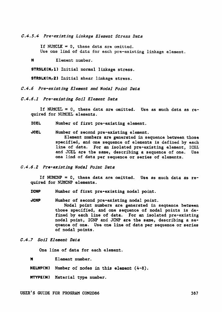
0.4.5.4 Pre-existing Linkage Element Stress Data
If NUMCLK = 0, these data are omitted.Use one lind of data for each pre-existing linkage element.
N Element number.
STRSLK(N•1) Initial normal linkage stress.
STRSLK(N,2) Initial shear linkage stress.
0.4.6 Pre-existing Element end Nodal Point Data
0.4.6.1 Pre-existing Soil Element Date
If NUMCEL = 0, these data are omitted. Use as much data as re-quired for NUMCEL elements.
ICEL Number of first pre-existing element.
JCEL Number of second pre-existing element.Element numbers are generated in sequence between those
specified, and one sequence of elements is defined by eachline of data. For an isolated pre-existing element, ICELand JOEL are the same, describing a sequence of one. Useone lind of data per sequence or series of elements.
0.4.6.2 Pre-existing Nodal Point Data
If NUMCNP = 0, these data are omitted. Use as much data as re-quired for NUMCNP elements.
IGNP Number of first pre-existing nodal point.
JCNP Number of second pre-existing nodal point.Nodal point numbers are generated in sequence between
those specified, and one sequence of nodal points is de-fined by each line of data. For an isolated pre-existingnodal point, ICNP and JCNP are the same, describing a se-quence of one. Use one line of data per sequence or seriesof nodal points.
0.4.7 Soil Element Date
One line of data for each element.
H Element number.
NELNPINI Number of nodes in this element (4-8).
MTYPEINI Material type number.
USER'S GUIDE FOR PROGRAM CON2D86 387

INP(N,1l Nodal point number I.
INP(N»2) Nodal point number II.
INPKN,3) Nodal point number III.
INP(N•4) Nodal point number IV.
INP(N,5) Nodal point number V.
INP(N,6) Nodal point number VI.
INP(N,7) Nodal point number VII.
INP(N,8) Nodal point number VIII.Soil element data must be read in sequence. The nodal
point numbers must be specified in the order I,II,III,IV,V,VI,VII,VIII as shown in the upper part of Figure C-1. Foran element with fewer than eight nodes, the nodal pointnumbers of the omitted nodes must be specified as zero.For triangular elements, the nodal point number III mustbe equal to the nodal point number IV, as shown at thebottom of Figure C-1. The locations of the integrationpoints, where pore pressures are calculated, are also shownin Figure C-1.
N = 1 for the first soil element.N = 2 for the second soil element.etc.
0.4.8 0onstruct1on Layer Element and Nodal Point Data
One line of data for each construction layer.If NLAY = 0, these data are omitted.
LN Construction layer number. Layer numbers increase upwardfrom the bottom.
NOMEL(LN,1l Smallest soil element number of the newly placed elementsin this layer.
NOMEL(LN,2) Largest soil element number of the newly placed elementsin this layer.
NOMEL(LN,3) Smallest bar element number of the newly placed bar ele-ments in this layer.
NONEL(LN•4) Largest bar element number of the newly placed bar ele-ments in this layer.
NOMNP(LN,1) Smallest nodal point number of the newly placed nodalpoints in this layer.
USER'S GUIDE FOR PROGRAM CON2D86 388
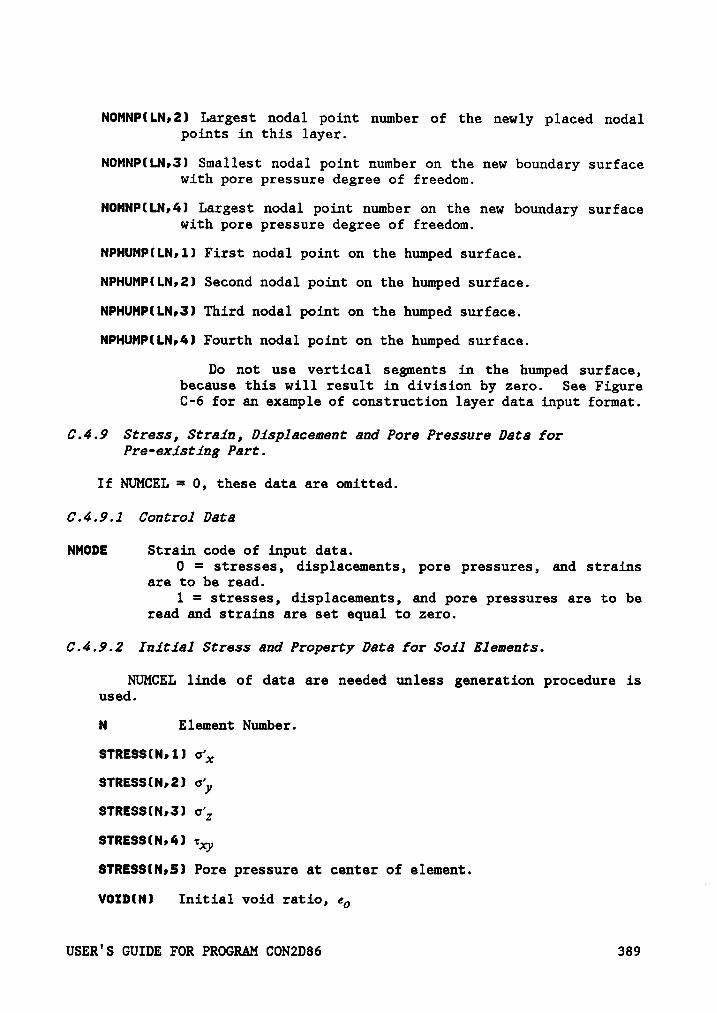
NOMNP(LN,2) Largest nodal point number of the newly placed nodalpoints in this layer.
NOMNP(LN,3l Smallest nodal point number on the new boundary surfacewith pore pressure degree of freedom.
NOMNP(LN•4) Largest nodal point number on the new boundary surfacewith pore pressure degree of freedom.
NPHUMP(LN;1) First nodal point on the humped surface.
NPHUMP(LN•2) Second nodal point on the humped surface.
NPHUNP(LN•3) Third nodal point on the humped surface.
NPHUMP(LN•6) Fourth nodal point on the humped surface.
Do not use vertical segments in the humped surface,because this will result in division by zero. See FigureC-6 for an example of construction layer data input format.
0.4.9 Stress, Strain, Displacement and Pore Pressure Data ferPre-existing Part.
If NUMCEL = 0, these data are omitted.
0.4.9.1 0ontrol Data
NNODE Strain code of input data.0 = stresses, displacements, pore pressures, and strains
are to be read.1 = stresses, displacements, and pore pressures are to be
read and strains are set equal to zero.
0.4.9.2 Initial Stress and Property Data for Soil Elements.
NUMCEL linde of data are needed unless generation procedure isused.
N Element Number.
STRESS(N,1) 0}
STRESS(N,2) 0}STRESS(N;3l 0}
STRESS(N•4) px}
STRE$S(N,5) Pore pressure at center of element.
VOID(N) Initial void ratio, eo
USER'S GUIDE FOR PROGRAM CON2D86 389
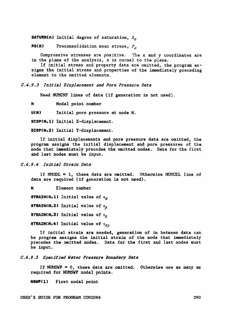
SATURN(n) Initial degree of saturation, S0
P0(Nl Preconsolidation mean stress, PO
Compressive stresses are positive. The x and y coordinates arein the plane of the analysis, z is normal to the plane.
If initial stress and property data are omitted, the program as-signs the initial stress and properties of the immediately precedingelement to the omitted elements.
0.4.9.3 Initial Displacement and Pore Pressure Data
Need NUMCNP lines of data (if generation is not used).
N Nodal point number
U(N) Initial pore pressure at node N.
DISP(N;1) Initial X-displacement.
DISP(N,2l Initial Y-displacement.
If initial displacements and pore pressure data are omitted, theprogram assigns the initial displacement and pore pressures of thenode that immediately precedes the omitted nodes. Data for the firstand last nodes must be input.
0.4.9.4 Initial Strain Data
If NMODL = 1, these data are omitted. Otherwise NUMCEL line ofdata are required (if generation is not used).
N Element number
$TRAIN(N;1) Initial value of sx
STRAIN(N,2) Initial value of eySTRAININ;3) Initial value of sz
STRAIN(N,4) Initial value of qxy
If initial strain are needed, generation of in between data canbe program assigns the initial strain of the node that immediatelyprecedes the omitted nodes. Data for the first and last nodes mustbe input.
0.4.9.5 Specified Water Pressure Boundary Data
If NUMSWP = O, these data are omitted. Otherwise use as many asrequired for NUMSWP nodal points.
NSWP(1) First nodal point
USER'S GUIDE FOR PROGRAM CON2D86 390
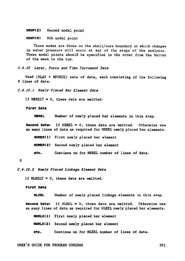
NSWPIZ) Second nodal point
NSWPINI Nth nodal point
These nodes are those on the shell/core boundary at which changesin water pressure will occur at any of the steps of the analysis.These nodal points should be specified in the order from the bottonof the mesh to the top.
0.4.10 Layer, Force and Time Increment Data
Need (NLAY + NFORCE) sets of data, each consisting of the following8 lines of data.
0.4.10.1 Newly Placed Bar Element Data
If NBRELT = 0, these data are omitted.
First Data
NBREL Number of newly placed bar elements in this step.
Second Data: If NBREL = 0, these data are omitted. Otherwise useas many lines of data as required for NBREL newly placed bar elements.
NUHBR(1) First newly placed bar element
NUMBRIZ) Second newly placed bar element
etc. Continue on for NBREL number of lines of data.
0
0.4.10.2 Newly Placed Linkage Element Data
If NLKELT = 0, these data are omitted.
First Data
NLKEL Number of newly placed linkage elements in this step.
Second Data: If NLKEL = 0, these data are omitted. Otherwise useas many lines of data as required for NLKEL newly placed bar elements.
NUMLK(1) First newly placed bar element
NUHLK(2) Second newly placed bar element
etc. Continue on for NLKEL number of lines of data.
USER°S GUIDE FOR PROGRAM CON2D86 391
6.4.10.3 Layer and Load 6ase 6ontro1 Data
NUMFC Number of nodal point forces in this load case.
NUMPC Number of distributed loads in this load case.
NUMBWP Number of nodal points subjected to a change in static waterpressure in this load case. (This number must be equal toor less than NUMSWP on the first control data line.
NUMBYP The number of elements which, during this load case, aresubmerged below a rising reservoir or which emerge above afalling reservoir.
NEWLAY 0 if there are no newly added elements in this step, greaterthan 0 if there are new elements added.
6.4.10.4 Buoyancy Force Data
If NUMBYP = 0, these data are omitted.
First Data
DELGAM Change in unit weight due to submergence or drawdown.
DELGAM = gv-y", for submerged elements. This value is nega-tive.
DELGAM = ym + yw—y_mt for elements which were below water be-fore drawdown and are above water after. This valueis positive.
second Data
NBYELII) Element number of first element which is submerged be-neath a rising water level or exposed above a fallingwater level.
NBYELIZI etc.
6.4.10.5 Nodal Point Force Data
If NUMC = 0, these data are omitted. Otherwise need NUMC linesof data.
N Nodal point number where force is applied
FXIN) X-component of force applied at N (+ to right).
FY(N) Y—component of force applied at N (+ up).
USER°S GUIDE FOR PROGRAM CON2D86~
392
0.4.10.6 Distributed Load Data
If NUMPC = 0, these data are omitted. Otherwise need NUMPC linesof data.
INODE Nodal point number at I
JNODE Nodal point number at J
PRESI Normal pressure at nodal point I
PRESJ Normal pressure at nodal point JDefinition of points I and J, and examples of data for
distributed load cases are shown in Figure C-7.
0.4.10.7 Reservoir Level Change Data
If NUMBWP = O, these data are omitted.
First Data
ISIGN ISIGN = 1 if water pressure acts in +x direction onstructure. ISIGN = -1 if water pressure acts in -xdirection.
LEVOLD Nodal point number at the same elevation as the oldwater level (before this load case).
NEHLEV Nodal point number at the same elevation as the newwater surface.
These data define changes in boundary pressure due to risingor falling water level. See Figure C-8 for an example of datafor a change in reservoir level.
0.4.10.8 Time Period Data
NSTEP Every load step is divided into NSTEP parts, each of whichis analyzed separately, to improve computational accuracy.
NTIME Length of time interval encompassed by this loading incre-ment.
Whenever it is desired to obtain output for various times with nochanges in loading, water levels or other conditions, save consolidation,another set of these data must be input.
USER°S GUIDE FOR PROGRAM CON2D86 393

Appendix D
USER'S GUIDE FOR PROGRAM CONSAX86
D.1 Introduction
The program CONSAX86 is an axisymmetric finite element computer pro-
gram for analysis of stresses, displacements and consolidation in satu-
rated and partly saturated earth masses. The program can be used to
analyze consolidation in soil mechanics problems that have an
axisymetric geometry. The program treats the coupled problem of defor-
mation and fluid flow, and can be used to calculate movements and pore
pressures under undrained, partly drained and fully drained conditions.
Reinforced soil structures can be analyzed using membrane elements (see
Appendix B).
CONSAX86 was originally developed by Chang and Duncan (1977) and was
later modified by D'Orazio and Duncan (1982). The program follows the
general programming concepts and solution techniques developed by Wilson
(1970) and Bathe and Wilson (1976). The present version incorporates a
membrane element to model reinforcement, and provides enhanced source
code documentation and efficiency.
USER'S GUIDE FOR PROGRAM CONSAX86 394

D.2 Program Operation
D.2.l Systems and Sign Convention
The global coordinate system is a right handed R-Z system with R in-
creasing to the right and Z increasing vertically.
Soil element and interface normal stresses are positive in compression
and negative in tension. The soil stresses are all effective stresses.
Positive pore pressures are compressive. Total stresses are obtained by
adding pore pressures at the center of elements to the effective soil
stresses.
Membrane element forces are output in a local coordinate system.
Radial force is positive if the member is in compression and negative if
in tension.
D.2.2 Storage Allocation
Dynamic storage allocation (Bathe and Wilson 1976) is used within the
program and storage is allocated at the time of execution. The storage
can be readily adjusted through the COMMON (A) statement in the source
code. Storage requirements are checked immediately after reading the
control data, and if insufficient, an error message printed detailing the
minimum storage requirements for the problem and execution is halted.
The equation-solving subroutines use only one-half of the full banded
stiffness matrix. Secondary storage (disk or tape storage) is used to
USER'S GUIDE FOR PROGRAM CONSAX86 395
minimize the amount of core storage required by solving the equations by
blocks (Wilson et al. 1974). The smaller the number of equations per
block, the greater is the required number of transfers between core and
secondary storage, and the more costly is the solution procedure. Thus,
the more storage allocation exceeds the minimum value, the larger is the
number of equations per block, and hence the shorter is the solution time.
0.2.3 Element Types
CONSAX86 has three types of elements as follows:
1. Soil elements are four·to-eight variable node, two-dimensional,
isoparametric elements as described by Bathe and Wilson (1976). Each
node may also have a pore pressure degree-of-freedom. Any number of
nodes from four to eight can be specified for each element. Trian-
gular shaped elements can be formed by superimposing nodes. The nodal
point numbers must be specified in the order I, II, III, IV, V, VI,
VII, VIII as shown in the upper part of Figure D-1. For an element
with fewer than eight nodes, the nodal point numbers of the omitted
nodes are set equal to zero, as shown in the bottom of Figure D-1.
For triangular elements, the nodal point number III must be equal to
the nodal point number IV.
2. Membrane elements are two node elements with radial stiffness only
(no flexural or shear resistance), and may be used to connect any two
nodal points.
USER'S GUIDE FOR PROGRAM CONSAX86 396
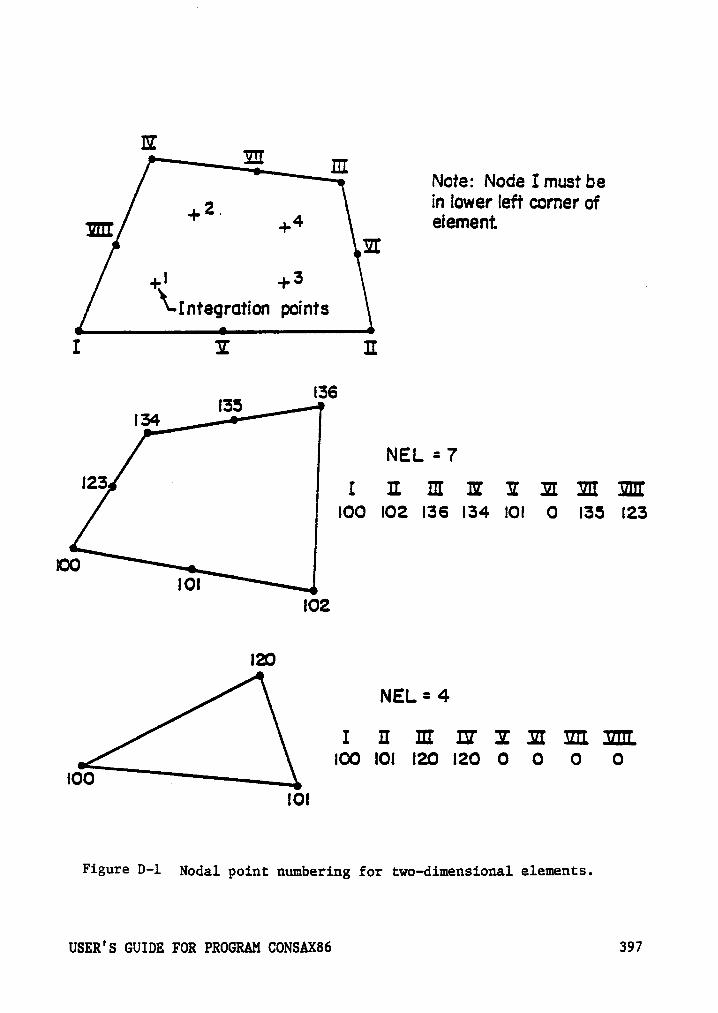
E E IHNote: Node Imust be
2 _ in lower left comer of‘*' +4 elementHI
+‘ +3 1\-Integration points
I I II
ISSI35
l34
NEL = 7'23 1 11 III II 2 :11 1111 mr
IOO lO2 l36 I34 IOI O IBS l23
IOOIOI
IO2
IE
NEL=4
I II III N I E III IIILIOO IOI l2O l2O O O O O
IOOIOI
Figure D-l Nodal point: numberiug for two-dimeusional elements.
USER°S GUIDE FOR PROGRAM CONSAXS6 l 397

3. Linkage elements may be used to represent interfaces between a
structure and adjacent soil or between zones within a soil mass. As
shown in Figure D-2, a linkage element connects two nodal points
called I and J, which may have identical coordinate values. The
stiffness of the linkage element represents the properties of a sec-
tion of the interface. The length and orientation of the section of
the interface represented by the linkage element are defined by two
nodal points called NI and NJ. The orientation of the interface in
along the line NI-NJ. The shear direction is parallel to NI-NJ, and
the normal direction is perpendicular to NI-NJ. The length of the
section of the interface is one-half of the distance from NI to NJ.
The examples of linkage element numbering shown in Figure D-3 illus-
trate how the orientations of linkage elements and the lengths of
sections of the interface they represent are defined in terms of nodes
I, J, NI and NJ.
0.2.4 Hasbes
A example mesh for analysis of a tank foundation is shown in Figure
D-4. The nodal points are numbered from left to right across each level.
Elements are numbered in the same way, with the element numbers increasing
from left to right in each layer and from the bottom up. For accurate
displacements, stresses, and pore pressures, loads should be applied in
six or more increments.
USER°S GUIDE FOR PROGRAM CONSAXB6 398
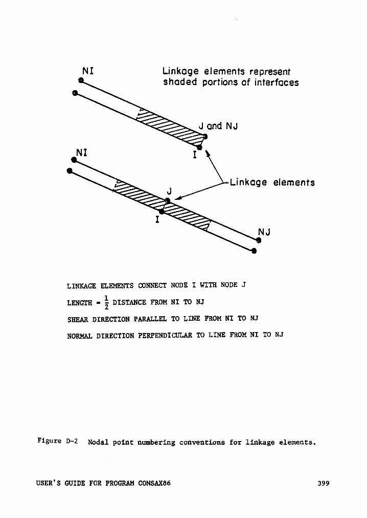
NI Linkoge elements representshcded portions of interfcces
J und NJ
NI I
Linkage elements- J
INJ
LINKAGE ELEMENTS CONNECT NODE I WITH NODE J
LENGTH DISTANCE FROM NI TO NJ
SHEAR DIRECTION PARALLEL TO LINE FROM NI TO NJ
NORMAL DIRECTION PERPENDICULAR TO LINE FROM NI TO NJ
Figure 1)**2 Nodal point numbering conventions for linkage elements.
USER'S GUIDE FOR PROGRAM CONSAX86 399
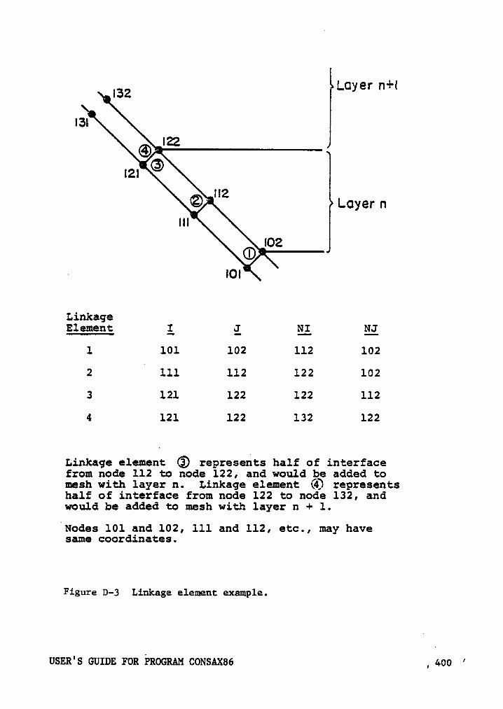
0 er n+I_. 132 L y
I3!
<)\I22I2! ©
H2® ‘ Loyer nIH
IO2
· IO!Il
LinkageElement L L QL QL
1 101 102 112 102
2L
111 112 122 102
3 121 122 122 112
4 121 122 132 122
Linkage element @ represents half of interfacefrom node 112 to node 122, and would be added tomesh with layer n. Linkage element G) representshalf of interface from node 122 to node 132, andwould be added to mesh with layer n + 1.
'Nodes 101 and 102, 111 and 112, etc., may havesame coordinates.
Figure D-3 Linkage element example.
USER'S GUIDE FOR FROGRAM CONSAXB6 , 400’
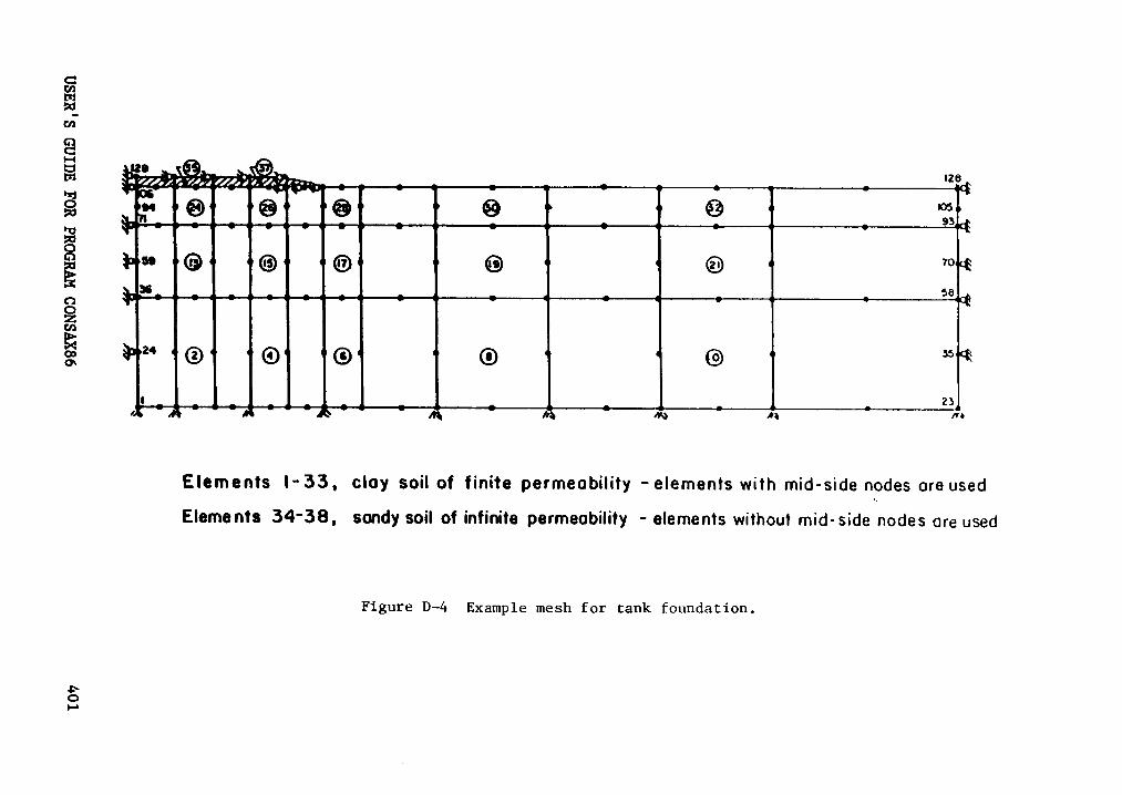
I•
·°°
•3-*}
:::~
{3
ÜkE
0O
en3
6'U
Oo
,¤
Ccu
<v73
Een
‘f’6
--E
{_
:O
ZE
S6
6©
6-
U,
•I.(
¢•·
4.:
·=S
6E
EQ
22
0ä
0E
u.:
IIé",;~
EB
T,rg
3S
“-E
Eg
ä¤
E
®ä
.s==
ä••-
_§nä
€.3
*6<r
-•
gI
an‘”
<u>~
H4
ä'§
ä’¤
@ E]!
E"’
E
S'°
'°IX
"‘ "‘
•\ @
@B
I~
5o
SS
I=
*°-3
•¤+§®
EE
J\•
"2
-5U-!
HJ
sß
llßl
.I-•
__
·
usER'sGUIDE
FORPROGRAM
CONSAX86401
Pre-existing elements in any configuration may be included within or
beneath the embankment. As shown in Figure D-5, the pre-existing part
of the mesh may be beneath the embankment, adjacent to the embankment,
or entirely within the final geometry of the complete embankment, and it
may consist of more than one part. The initial stresses, displacement,
and pore pressures may be generated by earlier analyses with CONSAX86 or
by hand calculations. The strains in the pre-existing part can be set
equal to zero by the program, or non-zero values can be read in by the
user, at the user°s option.
D.2.5 Increments
An increment may consist of the placement of a layer of fill on a
foundation, or of an application of loads to a mesh. Placement of a layer
of fill is simulated by applying forces to represent the weight of the
added layer. The layer being placed is assigned very small modulus values
to simulate the fact that a newly added layer of uncompacted fill has very
low stiffness. Each element in the new1y' placed layer is assigned
stresses consistent with the overburden pressure at its center. The
strains in the newly placed elements are set equal to zero, and taken as
the reference state of strain. For accurate results, it is best to add
only one layer of elements at a time, and in general, six or more layers
of elements in the mesh will provide reasonably accurate results.
A layer to be added in an increment is defined by specifying the first
and last elements to be added [NOMEL(LN,1) and NOMEL(LN,2)], the first
USER°S GUIDE FOR PROGRAM CONSAX86 402
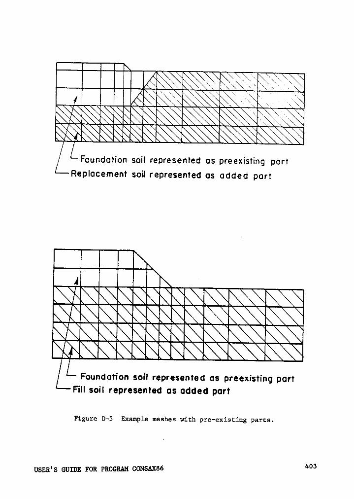
—IIII[§§§.
iii! IZZZZZEEIZZ EESÜSSEElllls
‘Y YE
‘V
NQ§§§§M§H§h§§¤~¤¤¤¤¤§¤¤¤m&!§§§B!&hS§§§§F§l§S§§!!!N§§§
Foundation soil represented as preexisting partFill soil represented as added part
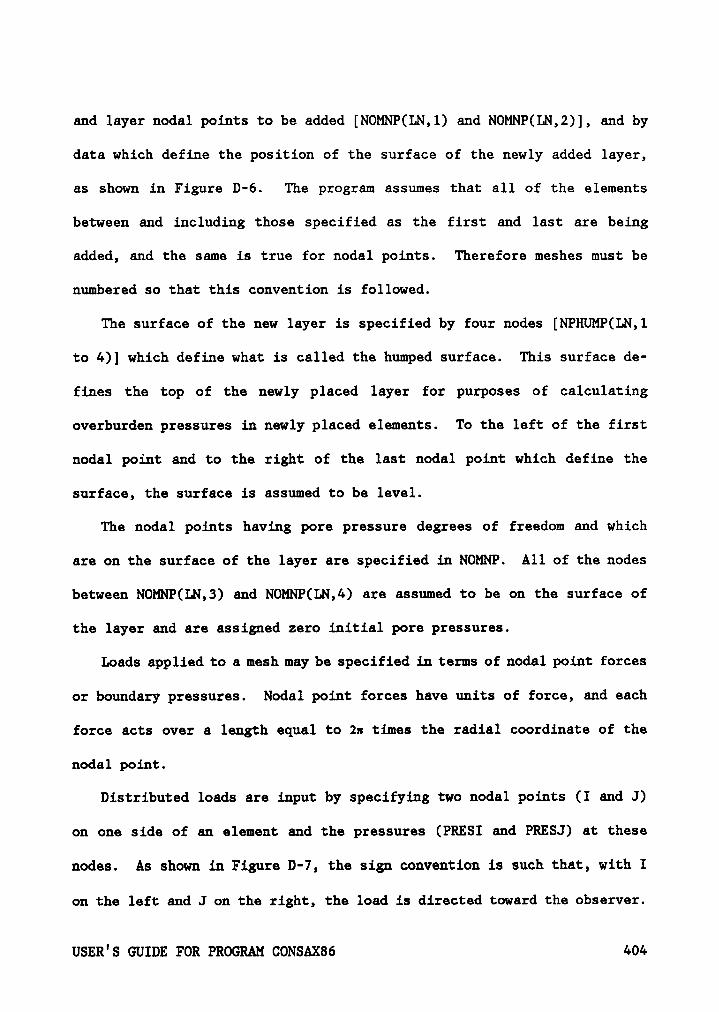
and layer nodal points to be added [NOMNP(LN,1) and NOMNP(LN,2)], and by
data which define the position of the surface of the newly added layer,
as shown in Figure D-6. The program assumes that all of the elements
between and including those specified as the first and last are being
added, and the same is true for nodal points. Therefore meshes must be
numbered so that this convention is followed.
The surface of the new layer is specified by four nodes [NPHUMP(LN,1
to 4)] which define what is called the humped surface. This surface de-
fines the top of the newly placed layer for purposes of calculating
overburden pressures in newly placed elements. To the left of the first
nodal point and to the right of the last nodal point which define the
surface, the surface is assumed to be level.
The nodal points having pore pressure degrees of freedom and which
are on the surface of the layer are specified in NOMNP. All of the nodes
between NOMP(LN,3) and NOMNP(LN,4) are assumed to be on the surface of
the layer and are assigned zero initial pore pressures.
Loads applied to a mesh may be specified in terms of nodal point forces
or boundary pressures. Nodal point forces have units of force, and each
force acts over a length equal to 2n times the radial coordinate of the
nodal point.
Distributed loads are input by specifying two nodal points (I and J)
on one side of an element and the pressures (PRESI and PRESJ) at these
nodes. As shown in Figure D-7, the sign convention is such that, with I
on the left and J on the right, the load is directed toward the observer.
USER°S GUIDE FOR PROGRAM CONSAX86 404
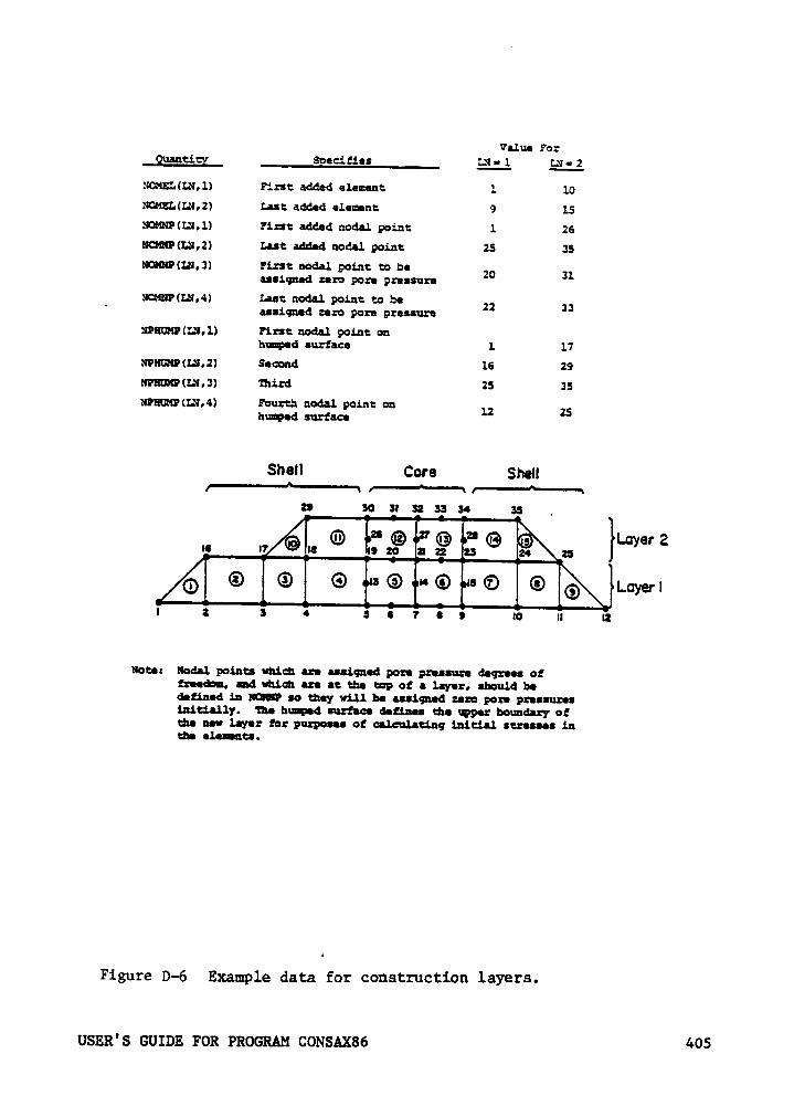
Value ForQgtig Soecifies T.N¤ l LN• 2
:l0:4£!„lI.N,l) Pirat added element l 10NOM!L(Iä|,2) Last added element 9 15!¤ßNP(Iäl,1) First added noda.1 point: 1 26B|CM!IP(IAl,2) Last added nodsl point ZS 35u¤MNP(¤l,3) First nodal point to be zo 31asalqned zero pore pressure
N¤M3IP(LbI,4) Iast nodal point to be 22 33' assiqned zero pore pressure
¤PE¤!0(L¤„l.) First nodal point onhumped surface l 17
NPHKI1P(1’AI,2) Second 16 29NPH¤KP(I2l,3) Third 25 35NPHUMHLN,4) Fourth nodal point cn 12 25huuped surface
Shell Core Shell
23 30 BI 32 33 34 35 „
®“
® ' @“
«¤ l-¤v¤•· 2IIAE @ @ Q ·—QQ~l 2 3 4 3 s 7 •
9 IO II I2
Nora: Nodal points which are aesiqued pore pressure deqrees offreedom, aedwlxlchareaethetapcfelayer, shouldbedefined in ww so they will be esslqned zero pore preesureslniually. The huqed surface defiaee the upper boundary ofthe new layer for purposes of calculadnq initial scressee inthe elesancs.
Figure D-6 Example data for construction layers.
USER'S GUIDE FOR PROGRAM CONSAX86 *+05

In this option, the program automatically calculates the radii of points
I and J and assigns the appropriate nodal point forces.
The data required to specify a constant non-zero pore pressure con-
dition is shown in Figure D-8. In this figure, the seepage from and the
expansion of a borehole due to water pressure is modeled. The number of
nodal points that have a constant non-zero pore pressure is NUMSWP. The
value of constant pore pressure is maintained for the duration of the load
case. A value of NUMBWP = 1 indicates that there are nodal points that
have a constant non-zero pore pressure for this load case.
D.3 Program Organization
The main program (CONSAXS6) reads and prints the control data and
monitors all operations by calling the subroutines in the specified order.
1. Subroutine LAYOUT controls the subroutines which read the input data.
Subroutine LAYOUT calls INFTNP to read and print nodal point data,
MATIN to read and print soil material property data, MEMBIN to read
and print membrane element data, LINKIN to read and print linkage
element data, PREXIN to read and print pre-existing element data,
ELEMIN to read and print soil element data, and CLBAND to calculate
the bandwidth for the problem. Storage requirements are calculated
and if the problem requires more storage, a message is printed and
execution halted.
USER°S GUIDE FOR PROGRAM CONSAX86 406
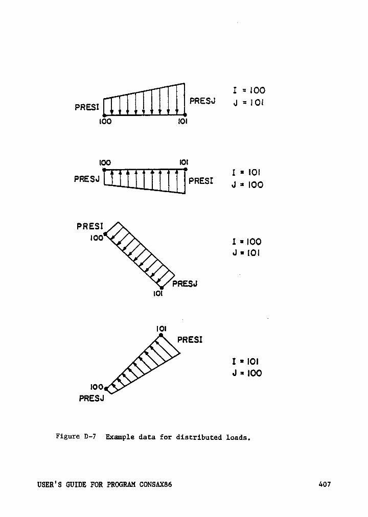
I = IOOPRESJ =Pass: J JOJ
Io¤ Ion
too IO!”I = IO!
PRESJ pagsx J S IOO
PRESI
'°° 1 = 100J = IO!
PRESJnon
IonV
PRESI
I = IOIJ = IOO
100A
PRESJ
Figure D-7 Example data for distributed loads.
usmvs GUIDE FOR pxocm CONSAXB6 407
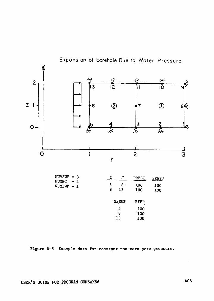
Expansion of BOr€hOl€ ÜUE Io WGTQF Pressure
Q
2
*
' • •
·
[I3 I2 n IO 6z I 6 @) 7 G) 6
’~
5 4 3 2 lO • • • •
O I 2 3I'
NUMSWP = 3 I J PRESI PRESJNUMPC = 2
5 8· 100 100NUMBWP = 18 13 100 100
NPSWP PFPR
5 1008 100
13 100
Figure D-8 Example data for constant non-zero pore pressure.
USER°S GUIDE FOR PROGRAM CONSAX86 **08
2. Subroutine INITL reads and/or calculates the initial values of
stresses, strains, displacements and pore pressures for pre-existing
elements and added layer elements.
3. Subroutine FORMB establishes the strain-displacement matrix for the
soil elements by calling BMATAX, which forms the strain-displacement
matrix for a four- to eight-node isoparametric, quadrilateral ele-
ment. BMATAX calls JACOBI to form the Jacobian, which calls SHAPE
to calculate the shape functions.
4. Subroutine CALBLK reads the control data for each increment and de-
termines the number of elements and nodal points being analyzed, the
number of elements and nodal points in the pre-existing part and added
layers, the number of equations, the number of equations in each
block, and the number of blocks for each increment.
5. Subroutine FVECT calculates nodal point forces due to weights of added
elements and reads and prints concentrated load data and boundary
pressure data.
6. Subroutine ELSTFF formulates the stiffness matrix for each element.
ELSTFF call STST to form the stress-strain relationship for the soil
elements and calls MODIFY to modify the load vector for each time
step. STST calls POICAL and LAMCAL to compute the current values of
Poisson's ratio and lambda, calls ELAST to calculate the elastic part
of the stress-strain relationship, and calls CAMCLY to calculate the
USER°S GUIDE FOR PROGRAM CONSAX86 _ 409

elasto-plastic stress-strain relationship. ELSTFF calls QK to cal-
culate the current compressibility and permeability of the pore fluid
in each element.
7. Subroutine ADDSTF forms the global stiffness matrix. The soil element
stiffness values are read from tape and the stiffness values for
membrane and linkage elements are found by calling MBSTIF and LKSTIF.
8. Subroutine TRIAFAC triangulizes the global stiffness matrix.
9. Subroutine REDVK back substitutes and solves the equations for dis-
placement and pore pressure.
10. Subroutine RESULT calculates the current values of stress and strain.
RESULT calls OUTPUT to print out the results.
USER°S GUIDE FOR PROGRAM CONSAX86 410
0.4 0ata Input Guide
0.4.1 Control Data
0.4.1.1 Heading Data (72A)
HEAD Title for program identification.
0.4.1.2 First Control Data
NUMELT Total number of soil elements in the complete mesh.
NUMNPT Total number of nodal points in the complete mesh.
NUMHAT Number of different soil material types.
NUMCEL Number of soil elements in the pre-existing part.
NUMCNP Number of nodal points in the pre-existing part.
NLAY Number of construction layer increments.
NFORCE Number of load increments after construction.
NUMSWP Total number of nodal points that have a constant non-zeropore pressure during any of the steps of the analysis.
0.4.1.3 Second Control 0ata
NMBELT Total number of membrane elements in the complete mesh.
NHHAT Number of different membrane material types.
NUMCMB Number of membrane elements in the pre-existing part.
NLKELT Total number of linkage elements in the complete mesh.
NLKHAT Number of different linkage material types.
NUMCLK Number ef linkage elements in the pre·existing part.
0.4.2 Nodal point and boundary condition data.
N Nodal point number.
R(N) R—coordinate (+ to the right).
ZINI Z-coordinate (+ up).
ID(H,1) Boundary condition code for displacement in the r-direction.
ID(N,2l Boundary condition code for displacement in the z-direction.
USER°S GUIDE FOR PROGRAM CONSAX86 411

ID(N,3) Boundary condition code for pore pressure.
Nodal points must be read in sequence. If nodal point data areomitted, the coordinates of a series of nodal points are generatedautomatically at equal spacing between those specified. The boundarycondition codes for the generated nodal points are set equal to theboundary condition codes for the previous nodal point. The first andlast points must be specified.
The boundary condition code convention is as follows:
r displacement always zero ID (N,1) = 1may be non-zero ID (N,1) = O
z displacement always zero ID (N,2) = 1may be non-zero ID (N,2) = 0
pore pressure always zero ID (N,3) = 1may be non-zero ID (N,3) = 0
0.4.3 Material Property Data
0.4.3.1 Units Conversion 0ata
PATH Atmospheric pressure expressed in the system of units usedin the problem.
GAHAH Unit weight of water expressed in the system of units used.
For example:
offUnit Atmospheric Unit weight
Length Weight Cohesion Stiffness Pressure of Water
ft ton/ft ton/ft ton/ft 1.058 0.0312ft kip/ft kip/ft kip/ft 2.116 0.0624ft lb/ft lb/ft lb/ft 2116.2 62.4
m ton/m ton/ft ton/ft 10.33 1.00M kN/m kN/m kN/m 101.3 9.807
cm kg/cm kg/cm kg/cm 1.033 0.001in lb/in psi lb/in 14.70 0.0361
0.4.3.2 Soil Material Properties
9 lines of data are required for each material.
H Material type number (MATNO).
USER'S GUIDE FOR PROGRAM CONSAX86 412
EMPR(H,1) Permeability code (PCODE).0.0 - for a material which is to be assumed infinitely
permeable, for example, the granular shell material in azoned earth dam.
1.0 - for a material which is not infinitely permeable,for example, the core material in a zoned earth dam.
EMPR(M.2) Unit weight (moist unit weight), y (GAMAW).
EMPR(M.3) Cam clay soil parameter, x (KAPPA).
EMPR(H,5) Intercept, pf (effective stress) (PRINTR).
EMPR(H,6) Slope, bqäbxüd (effective stress) (MTRIAX).
EMPR(H,9) Horizontal saturated permeability, gk (PERM).
EMPR(M,10) Vertical saturated permeability, gu (PERMZ).
EMPR(M,11) Degree of saturation at which the water begins to movefreely, ST
(SF).
EMPR(M.12) Initial void ratio, eo (VOID).
EMPR(M,13) Initial degree of saturation, So (SATURN).
EMPR(M,14l Pressure at which break in slope occurs,;rh?ak (PBREAK).
EMPR(M.15) Intercept after break, pr (PRINTR).
EMPR(H,16) Slope after break, bqäbxüd (MTRIAX).
EMPR(M,17l Preconsolidation pressure, Pb (mean normal stress) (PO).(PO).
EHPR(H,18) Tensile strength, c,(TENSTR).
The above values of initial void ratio, initial degree of satu-ration, and preconsolidation pressure are used only for materialproperties of elements that are not preexisting. The values of theseproperties for preexisting elements are submitted in data 9b.Second through fifth lines of data:
These data describe as many as 16 points on the pb ·l curve forthe material.
Second and third lines of data:
EMPR(M,31l Pressure, pb corresponding to the first X point.
EMPR(M,32l Pressure, pb corresponding to the second X point.
etc. continue for as many· points as needed to dexcribe theyo-—l curve. Two lines of data are required even in thecase where the pb-} curve is defined by eight or fewer
USER'S GUIDE FOR PROGRAM CONSAX86 413
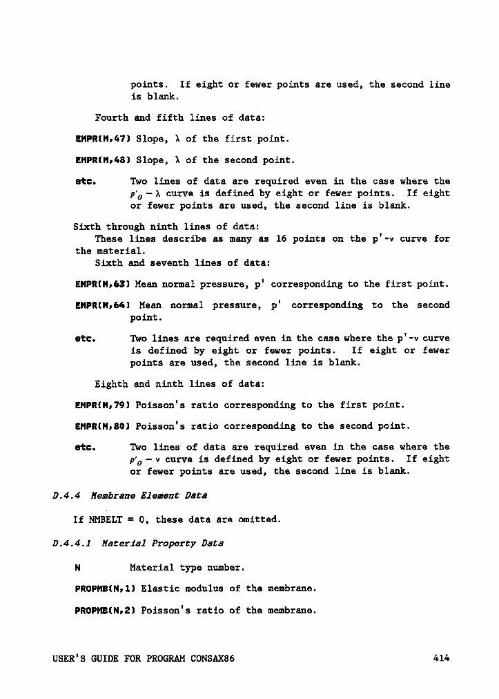
points. If eight or fewer points are used, the second lineis blank.
Fourth and fifth lines of data:
EMPR(M,471 Slope, X of the first point.
EMPR(M,48) Slope, X of the second point.
etc. Two lines of data are required even in the case where thepß-X curve is defined by eight or fewer points. If eightor fewer points are used, the second line is blank.
Sixth through ninth lines of data:These lines describe as many as 16 points on the p'-v curve for
the material.Sixth and seventh lines of data:
EMPR(H,63) Mean normal pressure, p' corresponding to the first point.
EMPR(H,66) Mean normal pressure, p' corresponding to the secondpoint.
etc. Two lines are required even in the case where the p°—v curveis defined by eight or fewer points. If eight or fewerpoints are used, the second line is blank.
Eighth and ninth lines of data:
EMPR(H,79) Poisson°s ratio corresponding to the first point.
EMPR(M,80l Poisson's ratio corresponding to the second point.
etc. Two lines of data are required even in the case where thepb-—v curve is defined by eight or fewer points. If eightor fewer points are used, the second line is blank.
D.4.4 Membrane Element Data
If NMBELT = 0, these data are omitted.
D.4.4.1 Material Property Data
N Material type number.
PROPMB(N,1l Elastic modulus of the membrane.
PROPMB(N•2) Poisson°s ratio of the membrane.
USER'S GUIDE FOR PROGRAM CONSAX86 414
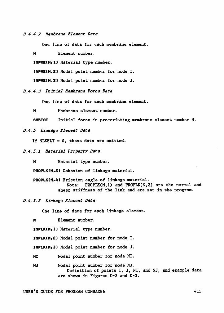
0.4.4.2 Membrane Element 0ata
One line of data for each membrane element.
M Element number.
INPMB(M,1) Material type number.
INPMB(M,2l Nodal point number for node I.
INPMB(M,3) Nodal point number for node J.
0.4.4.3 Initial Membrane Force Data
One line of data for each membrane element.
N Membrane element number.
SMBTOT Initial force in pre-existing membrane element number N.
0.4.5 Linkage Element Data
If NLKELT = 0, these data are omitted.
0.4.5.1 Material Property Data
N Material type number.
PROPLK(N,3l Cohesion of linkage material.Q
PROPLK(N,4) Friction angle of linkage material.Note: PROPLK(N,1) and PROPLK(N,2) are the normal and
shear stiffness of the link and are set in the program.
0.4.5.2 Linkage Element Data
One line of data for each linkage element.
H Element number.
INPLK(M,1) Material type number.
INPLK(M,2) Nodal point number for node I.
INPLK(M,3) Nodal point number for node J.
NI Nodal point number for node NI.
NJ Nodal point number for node NJ.Definition of points I, J, NI, and NJ, and example data
are shown in Figures D-2 and D-3.
USER°S GUIDE FOR PROGRAM CONSAX86 415
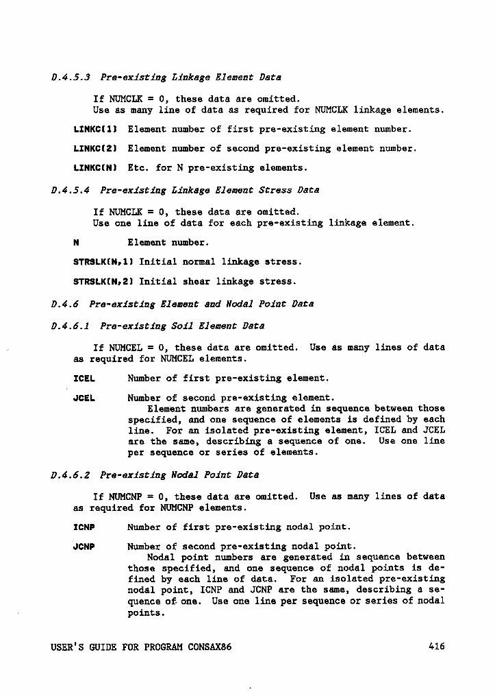
0.4.5.3 Pre-existing Linkage Element 0ate
If NUMCLK = 0, these data are omitted.Use as many line of data as required for NUMCLK linkage elements.
LINKG(1) Element number of first pre-existing element number.
LINKG(2l Element number of second pre-existing element number.
LINKGKNI Etc. for N pre-existing elements.
0.4.5.4 Pre-existing Linkage Element Stress Data
If NUMCLK = 0, these data are omitted.Use one line of data for each pre-existing linkage element.
N Element number.
STRSLK(N,1l Initial normal linkage stress.
STRSLK(N•2l Initial shear linkage stress.
0.4.6 Pre-existing Element and Nodal Point Date
0.4.6.1 Pre-existing Soil Element Data
„ If NUMCEL = 0, these data are omitted. Use as many lines of dataas required for NUMCEL elements.
IGEL Number of first pre-existing element.
JGEL Number of second pre-existing element.Element numbers are generated in sequence between those
specified, and one sequence of elements is defined by eachline. For an isolated pre-existing element, ICEL and JCELare the same, describing a sequence of one. Use one lineper sequence or series of elements.
0.4.6.2 Pre-existing Nodal Point 0ata
If NUMCNP = 0, these data are omitted. Use as many lines of dataas required for NUMCNP elements.
IGNP Number of first pre-existing nodal point.
JGNP Number of second pre-existing nodal point.Nodal point numbers are generated in sequence between
those specified, and one sequence of nodal points is de-fined by each line of data. For an isolated pre-existingnodal point, ICNP and JCNP are the same, describing a se-quence of one. Use one line per sequence or series of nodal
· points.
USER°S GUIDE FOR PROGRAM CONSAX86 416
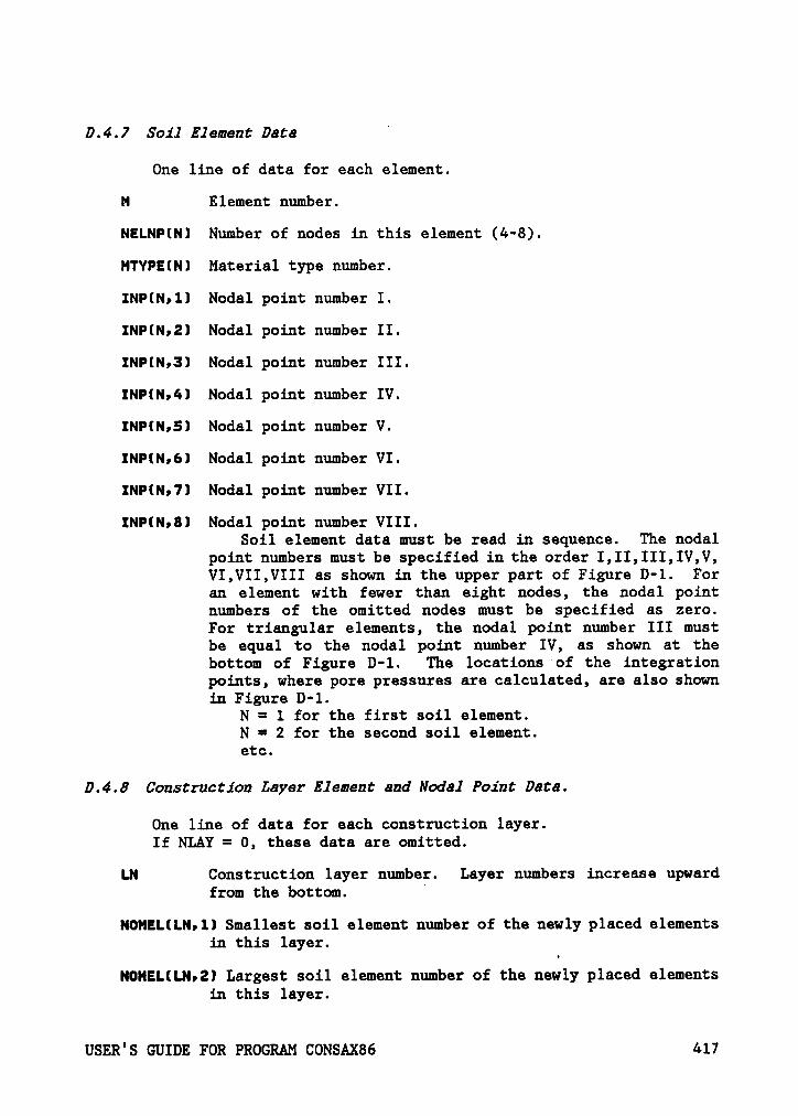
0.4.7 Soil Element 0ata‘
One line of data for each element.
N Element number.
NELNP(Nl Number of nodes in this element (4-8).
MTYPE(N) Material type number.
INP(N•1) Nodal point number I.
INP(N,2) Nodal point number II.
INPIN;3) Nodal point number III.
INP(N,4) Nodal point number IV.
INP(N,5) Nodal point number V.
INP(N,6) Nodal point number VI.
INP(N,7) Nodal point number VII.
INP(N,8) Nodal point number VIII.Soil element data must be read in sequence. The nodal
point numbers must be specified in the order I,II,III,IV,V,VI,VII,VIII as shown in the upper part of Figure D-l. Foran element with fewer than eight nodes, the nodal pointnumbers of the omitted nodes must be specified as zero.For triangular elements, the nodal point number III mustbe equal to the nodal point number IV, as shown at thebottom of Figure D-1. The locations of the integrationpoints, where pore pressures are calculated, are also shownin Figure D-1.
N = 1 for the first soil element.N = 2 for the second soil element.etc.
0.4.8 Construction Layer Element and Nodal Point Data.
One line of data for each construction layer.If NLAY = 0, these data are omitted.
LN Construction layer number. Layer numbers increase upwardfrom the bottom.
‘
NOMEL(LN,1) Smallest soil element number of the newly placed elementsin this layer.
NOMELlLN,2l Largest soil element number of the newly placed elementsin this layer.
USER°S GUIDE FOR PROGRAM CONSAX86 417
NOMEL(LN,3l Smallest membrane element number of the newly placedmembrane elements in this layer.
NOMEL{LN,4) Largest membrane element number of the newly placed mem-brane elements in this layer.
NOMNP(LN,1) Smallest nodal point number of the newly placed nodalpoints in this layer.
NOMNP(LN,2l Largest nodal point number of the newly placed nodalpoints in this layer.
NOMNP(LN,3l Smallest nodal point number on the new boundary surfacewith pore pressure degree of freedom.
NOMNP(LNp4) Largest nodal point number on the new boundary surfacewith pore pressure degree of freedom.
NPHUMP(LN,1) First nodal point on the humped surface.
NPHUMP(LN,2) Second nodal point on the humped surface.
NPHUMPlLN,31 Third nodal point on the humped surface.
NPHUHP(LN,4) Fourth nodal point on the humped surface.
Do not use vertical segments in the humped surface,because this will result in division by zero. See FigureD-6 for an example of construction layer data input format.
0.4.9 Stress, Strain, Displacement and Pore Pressure Data forPre-existing Part.
If NUMCEL = 0, these data are omitted.
0.4.9.1 Control Data
NMODE Strain code of input data.0 = stresses, displacements, pore pressures, and strains
are to be read.1 = stresses, displacements, and pore pressures are to be
read and strains are set equal to zero.
0.4.9.2 Initial Stress and Property Data for Soil Elements.
NUMCEL lines of data are needed unless generation procedure isused. UN Element Number.
8TRES$lN;1) 6}
STRESS(N,2) 6} ·
USER'S GUIDE FOR PROGRAM CONSAX86 418
STRESS(N•3) cg
STRESS(N,4) gz
STRESS(N,5l Pore pressure at center of element.
VOID(N) Initial void ratio, eo“
SATURN(n) Initial degree of saturation, S0
P0(N) Preconsolidation mean stress, PO
Compressive stresses are positive. The r and z coordinates arein the plane of the analysis, 6 is normal to the plane.
If initial stress and property data are omitted, the program as-signs the initial stress and properties of the imediately precedingelement to the omitted elements.
0.4.9.3 Initial Displacement and Pore Pressure Data.
Need NUMCNP lines of data (if generation is not used).
N Nodal point number
U(N) Initial pore pressure at node N.
DI$P(N,1) Initial R-displacement.
DISP(N,2l Initial Z-displacement.
If initial displacements and pore pressure data are omitted, theprogram assigns the initial displacement and pore pressures of thenode that immediately precedes the omitted nodes. Data for the firstand last nodes must be input.
0.4.9.4 Initial Strain Data. ‘
If NMODL = 1, these data are omitted. Otherwise NUMCEL lines ofdata are required (if generation is not used).
N Element number
STRAIN(N,1) Initial value of er{
STRAIN(N,2) Initial value of sz
STRAININ,3) Initial value of 89
STRAIN(N•4) Initial value of gz „
If initial strain are needed, generation of in between data canbe program assigns the initial strain of the node that immediatelyprecedes the omitted nodes. Data for the first and last nodes mustbe input.
USER'S GUIDE FOR PROGRAM CONSAX86 419
0.4.10 Layer, Force and Time Increment 0ata
Need (NLAY + NFORCE) sets of data, each consisting of the following8 lines of data.
0.4.10.1 Newly Placed Membrane Element 0ata. (skip if NMBELT = 0).
First Data
NMEL Number of newly placed membrane elements in this step.
Second Data: If NMBEL = 0, these data are omitted. Otherwise useas many lines of data as required for NMBEL newly placed membraneelements.
NUMHBII) First newly placed membrane element
NUMMBIZ) Second newly placed membrane element
etc. Continue on for NMBEL number of lines of data.
0
0.4.10.2 Newly Placed Linkage Element 0ata. (skip if NLKELT = 0).
First Data
NLKEL Number of newly placed linkage elements in this step.
Second Data: If NLKEL = 0, these data are omitted. Otherwise useas many lines of data as required for NLKEL newly placed membraneelements.
‘ NUMLK(1) First newly placed membrane element
NUMLKIZI Second newly placed membrane element
etc. Continue on for NLKEL number of lines of data.
0.4.10.3 Layer and Load Case Control Data
NUMFC Number of nodal point forces in this load case.
NUMPC Number of distributed loads in this load case.
NUMBHP 0 if there are no points that have a constant non-zero porepressure in this load case. 1 if there are points that havea constant non-zero pore pressure in this load case.
NEWLAY 0 if there are no newly added elements in this step, greaterthan 0 if there are new elements added.
USER°S GUIDE FOR PROGRAM CONSAX86 420
0.4.10.4 Nodal Point Force Data
If NUMTC = 0, these data are omitted. Otherwise need NUMTC linesof data.
N Nodal point number where force is applied
FR(N) R-component of force applied at N (+ to right).
FZINI Z-component of force applied at N (+ up).
0.4.10.5 Distributed Load Data
If NUMPC = O, these data are omitted. Otherwise need NUMPC linesof data.
INODE Nodal point number at I
JNODE Nodal point number at J
PRESI Normal pressure at nodal point I
PRESJ Normal pressure et nodal point JDefinition of points I and J, and examples of data for
distributed load cases are shown in Figure D—7.
0.4.10.6 Constaut Pore Pressure Data
If NUMBWP = 0, these data are omitted. Otherwise need NUMBWPlines of data.
NPSWP(Il Nodal point number at which pore pressure remains constant
PFPRII) Pore pressure at the nodal point.
0.4.10.7 Time Period Data
NSTEP Every load step is divided into NSTEP parts, each of whichis analyzed separately, to improve computational accuracy.
NTIHE Length of time interval encompassed by this loading incre-ment.
Whenever it is desired to obtain output for various times with nochanges in loading, water levels or other conditions, save consolidation,another set of these data must be input.
USER°S GUIDE FOR PROGRAM CONSAX86 421