1

Monitoring hydraulic processes with Automated time-Lapse

Electrical Resistivity Tomography (ALERT)

Suivi de processus hydrauliques in situ par tomographie de

résistivité électrique au cours du temps (ALERT)

O Kuras*, J D Pritchard, P I Meldrum, J E Chambers, P B Wilkinson, R D Ogilvy, G P

Wealthall

British Geological Survey, Kingsley Dunham Centre, Keyworth, Nottingham, NG12 5GG, United

Kingdom

*Corresponding author. Tel.: +44-115-936 3416; fax: +44-115-936 3261; e-mail: O.Kuras@bgs.ac.uk

2

Abstract

Hydraulic processes in porous media can be monitored in a minimally invasive fashion by

time-lapse electrical resistivity tomography (ERT). The permanent installation of specifically

designed ERT instrumentation, telemetry and information technology (IT) infrastructure

enables automation of data collection, transfer, processing, management and interpretation.

Such an approach gives rise to a dramatic increase in temporal resolution, thus providing new

insight into rapidly occurring subsurface processes. In this paper, we discuss a practical

implementation of automated time-lapse ERT. We present the results of a recent study in

which we used controlled hydraulic experiments in two test cells at reduced field scale to

explore the limiting conditions for process monitoring with cross-borehole ERT

measurements. The first experiment used three adjacent boreholes to monitor rapidly rising

and falling water levels. For the second experiment we injected a saline tracer into a

homogeneous flow field in freshwater-saturated sand; the dynamics of the plume were then

monitored with 2D measurements across a 9-borehole fence and 3D measurements across a

3×3 grid of boreholes. We investigated different strategies for practical data acquisition and

show that simple re-ordering of ERT measurement schemes can help harmonise data

collection with the nature of the monitored process. The methodology of automated time-

lapse ERT was found to perform well in different monitoring scenarios (2D/3D plus time) at

time scales associated with realistic subsurface processes. The limiting factor is the finite

amount of time needed for the acquisition of sufficiently comprehensive datasets. We found

that, given the complexity of our monitoring scenarios, typical frame rates of at least 1.5–3

images per hour were possible without compromising image quality.

Keywords

Time-lapse electrical resistivity tomography, automated remote geophysical monitoring,

hydraulic processes, tracer test, cross-borehole tomography

3

Résumé

Les processus hydrauliques dans les milieux poreux peuvent être suivis avec un minimum de

perturbation par la tomographie de resistivité électrique au cours du temps (ERT). Une station

permanente d’instrumentation ERT spécialement adaptée, de télémétrie et de technologie de

l’information permet l’automatisation de la collecte, du transfert, du traitement, de la gestion

et de l’interprétation des données. Cette approche conduit à une augmentation remarquable de

la résolution temporelle, ce qui donne une nouvelle information sur les processus évoluant

rapidement dans le sous-sol. Dans cet article, nous présentons une mise en oeuvre pratique de

l’ERT temporelle automatisée. Nous présentons les résultats d’une étude récente, où nous

avons utilisé des expériences hydrauliques contrôlées dans deux cellules de test à une échelle

de terrain réduite afin d’explorer les conditions limitantes d’un suivi des processus par des

mesures d’ERT entre forages. La première expérience a utilisé trois forages adjacents pour

observer des niveaux d’eaux montant et descendant rapidement. Dans la seconde expérience,

nous avons injecté un traceur salin dans un champ d’écoulement homogène dans des sables

saturés en eau douce; la dynamique du panache a ensuite été observée par des mesures en 2D

à la traversée d’une barrière de neuf forages et par des mesures en 3D au sein d’un maillage

de 3×3 forages. Nous avons examiné différentes stratégies pratiques de collecte de données et

montrons qu’une simple réorganisation des schémas de mesures d’ERT peut aider à

harmoniser la collecte de données avec la nature du processus étudié. La méthodologie de

l’ERT temporelle automatisée s’est avérée très performante dans différents scénarios de suivi

(2D/3D temporels) à des échelles de temps associées à des processus réalistes se déroulant

dans le sous-sol. Le facteur limitant est la durée de temps finie nécessaire à l’acquisition

d’ensembles de données suffisamment complets. Nous avons trouvé que, étant donné la

complexité de nos scénarios de suivi, des vitesses typiques de clichés d’au moins 1,5-3

images par heure étaient possibles sans compromettre la qualité des images.

Mots clefs

Tomographie de résistivité électrique temporelle, suivi géophysique automatique à distance,

processus hydrauliques, test de traceur, tomographie entre forages.

4

1 Introduction

Time-lapse electrical resistivity tomography (ERT), or the analysis of electrical images

derived at specific intervals in time from spatially distributed resistance data, provides the

capability to monitor hydraulic processes in porous media in a minimally invasive fashion by

capturing the temporal conductivity variations associated with them. This increasingly

popular technique has obvious applications in environmental monitoring, civil and process

engineering, waste management and the growing field of hydrogeophysical research. Recent

examples have included the monitoring of:

• aquifers during tracer tests [3, 14, 20],

• infiltration into the unsaturated zone [9],

• coastal zones and saline intrusion [19, 23],

• embankment dams [13, 21], levees and other geotechnical infrastructure, and

• landfills [10, 11].

Traditionally, ERT monitoring is often carried out by means of manual repeat surveys, in

which electrodes are installed temporarily for the duration of the measurements. The

permanent installation of in-situ sensors along with the addition of telemetry have proven to

be particularly attractive as ERT data acquisition can thus be initiated, controlled and

manipulated remotely. This step has facilitated a significant evolution in methodology by

enabling a high degree of automation for ERT data transfer, processing, management and

interpretation [7, 16, 19, 25]. The power of such an approach lies in the dramatic increase in

temporal resolution compared to both manual repeat surveys and manually controlled

permanent installations, thus providing the potential for new insight into rapidly occurring

subsurface processes. We refer to this concept as automated time-lapse electrical resistivity

tomography (ALERT) and have recently developed dedicated instrumentation, telemetry and

IT infrastructure for its practical implementation.

Better hydrogeophysical characterisation is desirable for a wide range of complex and rapidly

occurring subsurface processes, such as sharp variations in saturation levels or changes in

aquifer properties associated with groundwater movement, solute transport or contaminant

migration. An example of a highly complex process is leachate circulation in landfill sites,

which involves rapid movement of fluids (multiphase flow) due to hydraulic forcing and

saturation changes caused by temperature/pressure variations, hydrochemical alteration and

landfill gas generation. However, the acquisition of resistance data and ERT image generation

5

invariably requires a finite amount of time, which affects image quality and imposes a limit

on the rates of change that can be captured with ALERT monitoring. A common fundamental

requirement for all rapid monitoring applications is the need to optimise the style of ERT data

acquisition by balancing the complexity of measurement schemes (and hence the acquisition

time) against spatial and temporal accuracy and resolution.

In this paper, we present our implementation of the ALERT concept and discuss the results of

a recent study exploring the limiting conditions for successful monitoring of a series of

generic controlled hydraulic experiments with cross-borehole ERT measurements. While a

number of recent studies have focussed on hydrogeophysical aspects, aquifer transport

characteristics and the quantification of ERT monitoring results in an attempt to derive

hydraulic properties [14, 20], we concentrate here on the generic aspects of ERT monitoring

and the necessary technology. ALERT instrumentation, telemetry, data management and

processing workflow are described in the first part of the paper. The second part describes

how we have used specifically designed hydraulic test cells at reduced field scale to validate

the ALERT concept by emulating typical subsurface processes. These included (1) the

temporal evolution of water levels and surface infiltration into the unsaturated zone and (2)

the migration of fluids with anomalous electrical properties, for example as caused by

advancing pollution plumes or leachate recirculation in landfilled waste. The performance of

ALERT in different monitoring scenarios (2D/3D plus time) was also assessed.

2 The ALERT geophysical monitoring concept

At the heart of the ALERT monitoring concept is a core measurement system and data logger

that is capable of autonomously scheduling, collecting and storing time-lapse electrical

imaging data. This instrumentation is installed at a remote site and links seamlessly with other

ALERT components that we have developed, including autonomous and environmentally

friendly power supply solutions, long-distance telemetry, a relational data management

system, web delivery and deployment options that allow remote operation in a reliable and

secure manner.

2.1 Instrumentation

The core ALERT measurement system implements the same functionality as manual multi-

electrode ERT survey equipment that is now widely available commercially. It supports a

range of geoelectrical measurement types, including resistance, induced polarisation, and self-

potential across ten input channels. The system has been designed for battery operation (12 or

24 V) and grid power, solar panel or wind turbine charging options are available for

6

autonomous operation in remote locations. Open system architecture allows for scalability

(virtually any practical number of electrodes can be addressed via switching modules) and the

integration of alternative environmental sensor types (e.g. temperature, pressure, pH). User-

adjustable acquisition parameters (e.g. duty cycle) and measurement criteria add to the

flexibility of the ALERT system. Its on-board memory allows the storage of multiple

command files and measured datasets prior to external download.

2.2 Remote operation and telemetry

In its default mode of deployment, the ALERT system is housed in a secure enclosure (e.g.

instrumentation kiosk) on the site to be monitored. The permanently installed sensor network

is typically buried below the ground surface [19] and attached to the system inputs. Between

data acquisition cycles, batteries are recharged while the system is idle and no measurements

are scheduled. The ALERT system utilises a serial protocol to allow bidirectional

communication with customised control software via a direct PC connection, PSTN, GSM, or

satellite modem. Protocol tunnelling enables the communications link to be established via

local area networks, cellular networks (GPRS, HSDPA) or the Internet. This form of

telemetry enables rapid and efficient transfer of all setup parameters, command files and

measurement data. The control software is used to schedule, monitor and retrieve ALERT

measurements from one or multiple field systems on one or multiple remote sites.

2.3 Data management

The automation of geophysical time-lapse processing and inversion requires a high degree of

consistency and integrity of measured datasets. This basic prerequisite demands a highly

structured approach to handling data. A relational data model was developed to capture the

full complexity of time-lapse electrical monitoring data and to allow efficient databasing. On

the one hand, this model takes into account the inherent relationships between the measured

parameters (e.g. resistances, potentials for SP or decay curves for IP) and any metadata

associated with the particular dataset, such as for example site details, electrode geometry and

acquisition settings. Each dataset generated by the ALERT instrumentation contains

associated metadata to ensure safe and consistent transfer, processing and storage. On the

other hand, the data model provides the framework for time-lapse processing and the analysis

of interdependence between subsequent datasets.

We have established a data management system on a dedicated server, handling all

communication, scheduling of data acquisition, data retrieval from field systems, processing

and storage. A separate machine handles the processor-intensive numerical inversions.

7

2.4 Processing workflow and delivery of results

Once a dataset has been retrieved, it is automatically uploaded to the database. We then apply

suitable pre-processing algorithms to screen for outliers and noisy data. Subsequently, the

dataset is exported to a resistivity inversion algorithm, which generates a resistivity model as

appropriate, using relevant constraints and a-priori information. After the inversion has been

completed, results are once again uploaded to the database. Finally, a suitable graphical

representation of the resulting resistivity model (e.g. contour map, colour image, 3D

tomogram) is generated and uploaded to the web server. End users as well as administrators

interact with the data management system through a customised web-based interface, which

offers a range of options for querying, manipulating and retrieving monitoring information.

2.5 Optimisation of data acquisition and interpretation strategies

A powerful argument in favour of automated time-lapse monitoring is that it provides an

opportunity to use previously collected data for the continuous (and automated) improvement

of the strategies for acquiring and interpreting new data. This can be achieved by gradually

optimising the set of electrode array configurations used for data collection [24, 28], based

upon the results obtained from previous measurements. Ultimately, it is our aim to integrate

such an approach into the ALERT monitoring concept.

3 Experimental validation with hydraulic experiments

3.1 Test site design and experimental scenarios

We have designed and installed a hydrogeophysical test facility within the grounds of the

BGS headquarters in Keyworth (Nottinghamshire, UK), which has been continuously

upgraded since the summer of 2004. The site comprises two test cells, which facilitate a range

of generic hydraulic experiments at reduced field scale. In this paper we focus on two basic

experimental scenarios that we have monitored using the ALERT methodology:

Liquid levels/phreatic surface. In this scenario, rapid variations in liquid levels were

monitored using time-lapse cross-borehole ERT. Conventional hydraulic level measurements

in monitoring wells only provide information about the immediate vicinity of the borehole,

whereas cross-hole ERT can yield estimated properties of the formation between the

boreholes. An example of where this can be useful is the landfill context, where leachate

levels in the waste mass may vary considerably between monitoring points and complex

internal structure of the waste and engineered barriers may result in perched leachate tables.

8

Lateral tracer transport. In this scenario, rapid lateral transport of a conductive tracer fluid in

a saturated medium was monitored using cross-hole ERT along a multi-borehole fence. This

scenario can be regarded as a proxy for a wide variety of hydraulic processes, such as solute

transport, contaminant migration or leachate recirculation.

3.1.1 Test cell 1

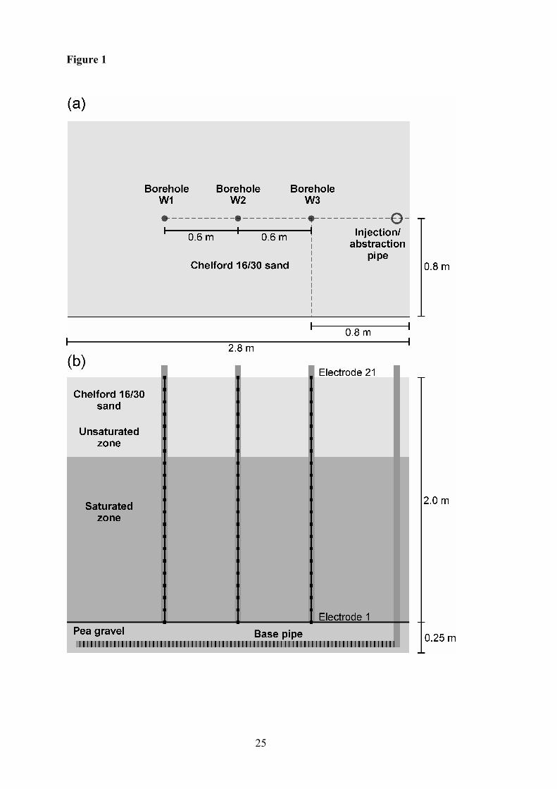
Cell 1 comprises a large pit with a depth of 2.25 m (void space approximately 10 m3),

excavated into made ground and lined with plywood (Figure 1). The surrounding material

consists of reworked mudstones of the Cropwell Bishop Formation (Mercia Mudstone Group,

[12]), which are rich in clay and of low permeability, thus providing a suitable natural barrier

for the purposes of our experiments. Water inflow is provided through a slotted horizontal

pipe at the base of the cell, which was installed in a bed of pea gravel to allow controlled

water injection and abstraction from the cell base. Three simulated boreholes were installed in

a central imaging plane, consisting of stainless steel electrodes mounted at 0.1 m separations

on the outside of PVC pipes (34 mm diameter). This design is the scale equivalent of standard

monitoring well completions typically used in landfill sites. Each well was equipped with 21

electrodes, resulting in a total of 63 electrodes useable for monitoring. Multicore cables were

used to connect individual electrodes with the switching modules of the ALERT monitoring

system located in the vicinity of the cell.

The void was backfilled with washed and graded high silica sand (Chelford 16/30, effective

grain size d10 = 0.53 mm) to provide a well-defined background medium with reasonably

homogeneous hydraulic properties. A hydraulic system was installed in the cell to enable the

controlled saturation of the sand volume and variation of liquid levels. The cell is connected

to the water mains via a header tank and is filled and emptied through a combination of low-

power submersible pumps. High and low water submersible sensors control the filling process

and allow the establishment and retention of accurate liquid levels in the cell. Independent

control is provided by conventional water level measurements using a water level indicator or

pressure transducer.

3.1.2 Test cell 2

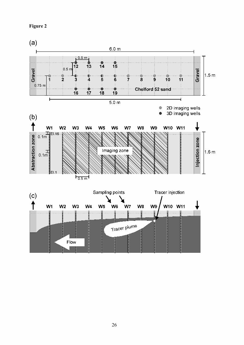
Cell 2 was established in the vicinity of Cell 1 and comprises an unlined elongated trench

(6.0 m × 1.5 m × 1.6 m, void space = 14.4 m3), which allows the creation of an approximately

uniform horizontal flow field by imposing a hydraulic gradient on the saturated volume. A

more complex layout with 19 simulated wells was chosen, facilitating the use of both 2D and

3D imaging configurations (Figure 2). A central fence of 11 wells forms a central imaging

plane in the trench, with a matrix of 3×4 wells creating a 3D imaging volume offset from the

9

centre of the cell. Each well was equipped with 16 electrodes mounted at 0.1 m separations.

Electrical connectivity was established in the same way as in Cell 1. Cell 2 was backfilled

with the same type of sand as Cell 1, except that a finer grade was used (Chelford 52, average

grain size 0.267 mm). This was done in order to achieve a suitably low horizontal flow rate

through the trench, so as to avoid image blur during ERT acquisition. A system of pumps and

level sensors was installed, providing precise control over the hydraulic gradient along the

trench, which is an essential prerequisite for solute transport experiments. A number of wells

in Cell 2 were equipped with multilevel sampler ports [6] made of thin PVC tubing to allow

in situ sampling of pore water from the saturated zone across a range of depths. All wiring

and services were routed to a nearby portacabin, which served as a field laboratory and

permanent shelter. A prototype ALERT system was installed in the portacabin along with

wireless communication in order to simulate remote conditions on a field site.

3.2 Experiment 1: monitoring liquid levels

The first experiment used time-lapse ERT across the three instrumented boreholes in Cell 1 to

monitor rapidly rising and falling water levels in the cell. Although the test was repeated

several times, the data presented in this paper are the result of measurements carried out on 31

August 2006.

3.2.1 Experimental setup, pumping regime and time scales

Initially the cell was filled with tap water and the sand saturated to a level of “high water”

approximately 0.5 m below ground level (bgl). A constant pumping rate was employed, which

resulted in a rate of water level change in Cell 1 of around 0.35 m/h during both injection and

abstraction. Using this constant pumping rate, the cell was first emptied to a level of “low

water” of 1.9 m bgl, where submersible level sensors were set to switch off the abstraction

pumps and activate injection, thus refilling the cell again at the same constant rate. A

corresponding set of sensors at the “high water” level ensured that pumping was reversed

again once the cell was fully saturated, thus completing a full pumping cycle. This alternating

pumping regime was maintained over a period of at least 24 hours, so that the cell was

drained and refilled at least five times. One half-cycle (either falling or rising water levels)

lasted approximately 4.5 hours.

A key question in ERT monitoring is whether time-lapse images are able to resolve in

sufficient detail the spatial property changes associated with the process monitored. In our

experiment, the expected change related to the retreat or advance of the phreatic surface,

which in practice takes the form of a capillary fringe (or tension-saturated zone) above a

10

notional water table [8]. The degree of saturation of the capillary fringe decreases gradually

from the water table upwards, implying a gradational change in electric properties [2]. The

capillary forces and hence the extent of the rise are affected by the pore radius of the medium

and the surface tension of the liquid. The Washburn equation describes capillary flow for the

simplified case of cylindrical capillaries [26], but is found to be applicable to many porous

media in general:

trthηθγ

2cos)( = , (1)

where t denotes the time, h the height of rise, γ the surface tension of the liquid, r the radius of

the capillary pore, θ the wetting angle, and η the viscosity of the liquid. The Washburn

equation refers to a steady process, where the capillary force is compensated by gravity and

viscous drag. Equation (1) corresponds to the short-time limit (t→0) and represents the

asymptotic solution of the fundamental partial differential equation of Newtonian dynamics

applicable to the problem [29]. In the long-time limit (t→∞), the capillary liquid will rise to a

stationary level h∞, established by the equilibrium between gravity and capillary forces:

grh

ρθγ cos2

=∞ . (2)

Here, ρ denotes the liquid density and g the gravitational acceleration. Assuming γ = 0.073

N/m for water, α = 0, ρ = 998 kg/m3 at 20°C, g = 9.8 m/s2 and r ≈ 0.2 d10, the estimated

maximum capillary rise for our experiment in Cell 1 is likely to be h ≈ 0.14 m. This compares

favourably with the fundamental vertical resolution of cross-hole ERT monitoring in our

experiments, which was expected to be of the order of the electrode spacing on the simulated

wells (0.1 m). We therefore expected to be able to resolve a transition zone of 1–2 electrode

spacings in the ERT images between the phreatic and vadose parts of the cell. The estimated

timescale of capillary flow over this distance of 0.14 m according to equation (2) is

approximately 5 s (η ≈ 10-3 Pa⋅s at 20°C). This is negligible against the timescale of pumping

(see above) and that of ERT measurements on a crosshole imaging plane. Consequently, time-

lapse image blur due to capillary-delayed flow was deemed unlikely.

3.2.2 Array configurations and acquisition strategies

ERT measurements were made using cross-borehole configurations spanning all three

simulated wells (W1, W2, W3, cf. Figure 1). The imaging plane comprised two neighbouring

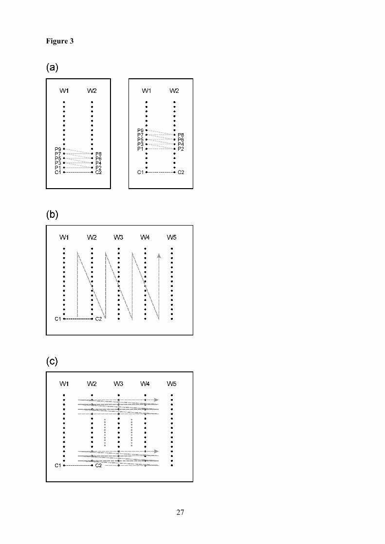
inter-borehole panels (W1-2 and W2-3). In accordance with Zhou and Greenhalgh [30], we

opted for the symmetrical bipole-bipole array as the preferred array geometry for all crosshole

measurements. For this geometry, one current electrode and one potential electrode are placed

11

in each of two wells. In order to keep acquisition time to a minimum, we considered only

measurements where current and potential bipoles were approximately horizontal, i.e. C1 and

C2 (as well as P1 and P2) were placed at similar depths (Figure 3a). This was deemed adequate

as previous studies had shown that 2D crosshole resistivity models could be sufficiently well

constrained if measurements were made on horizontal bipoles only [5, 15, 27].

One important objective of this study was to assess the impact of using multiple panels for

data acquisition on tomographic reconstruction and image quality. We devised two

complementary measurement strategies in order to evaluate the effect of measurement

sequences and timings on image blur during monitoring. The first strategy (referred to as

panel-by-panel) aims to complete individual inter-borehole panels before moving to a

neighbouring panel (Figure 3b). With regard to the overall imaging plane, all measurements at

a particular lateral position are therefore made at similar times. The second strategy gives

priority to interleaved measurements across all neighbouring panels. Measurements at equal

depths are therefore made at similar times (Figure 3c). In both cases, resistance measurements

commence at the bottom of a panel and current and potential dipoles are then moved up

successively along the boreholes. For each current injection, the set of measurements with the

shorter separation between current and potential dipoles (Figure 3a, left-hand diagram) is

carried out first; this is followed by the set with longer separations (Figure 3a, right-hand

diagram).

3.2.3 Data processing and inversion

The ALERT system uses switched DC source signals with self-adapting current settings.

Input currents between 4 and 112 mA were employed in Cell 1, depending on the local

contact resistance, which is a function of saturation state. We found that comprehensive

measurement schemes covering the complete imaging plane typically required 480 individual

resistance measurements. Using current pulse widths of 800 ms and minimal stacking of two

readings per measurement, these schemes took approximately 15–17 min to complete. Data

acquisition was therefore scheduled every 20 min and automatically performed by the

ALERT system. Individual datasets were transferred via telemetry to the data management

system for processing. Datasets were screened for quality, but were found to require only

moderate pre-processing owing to the tightly controlled experimental setup with favourable

noise conditions. In almost all occasions, all individual measurements could be retained.

Datasets were then inverted using a 2D crosshole least-squares smoothness-constrained

algorithm (Res2dinv, [17]).

12

3.2.4 Results and discussion

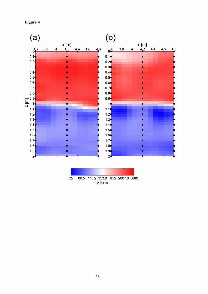
Figure 4 shows a direct comparison between two images acquired with the panel-by-panel

(Figure 4a) and interleaved (Figure 4b) measurement strategies. The tomograms cover the full

imaging zone comprising both inter-borehole panels (W1-2 and W2-3). Both datasets were

collected at identical water levels while the cell was being emptied. The resistivities range

from around 20 Ωm (blue) to over 5,500 Ωm (red), with intermediate resistivities (~300–

1,000 Ωm) displayed as faint blue, white or faint red colours. The model discretisation we

have chosen comprises 480 model cells in 40 layers (5 cm thickness) and 12 columns (10 cm

width). The images show a very clear separation between the water-saturated sand at the

bottom of the test cell (phreatic zone) and the dry or partially saturated sand at the top of the

cell (vadose zone). The water table and overlying capillary fringe are represented by a sharp

transition from low (blue) to high resistivities (red).

The two strategies give significantly different results and the image distortion caused by the

panel-by-panel approach is clearly visible. During the time it took for an individual borehole

panel to be measured (approximately 7–8 min), the water level in Cell 1 had changed by an

estimated 0.05 m, given the average pumping rate of 0.35 m/h. Although this change is

nominally smaller than the anticipated fundamental image resolution of 0.1 m, the impact on

the inverted images is obvious. The result of the panel-by-panel acquisition is a skewed

image, in which the transition zone is noticeably offset between the two neighbouring panels.

For the interleaved scheme, the resulting image shows no distortion as the transition zone is

traversed on both panels within a very short period of time. These results demonstrate the

sensitivity of the bipole-bipole crosshole measurement scheme to variations in the sharp

vertical contrast in electrical properties. All further measurements were therefore carried out

with the interleaved strategy.

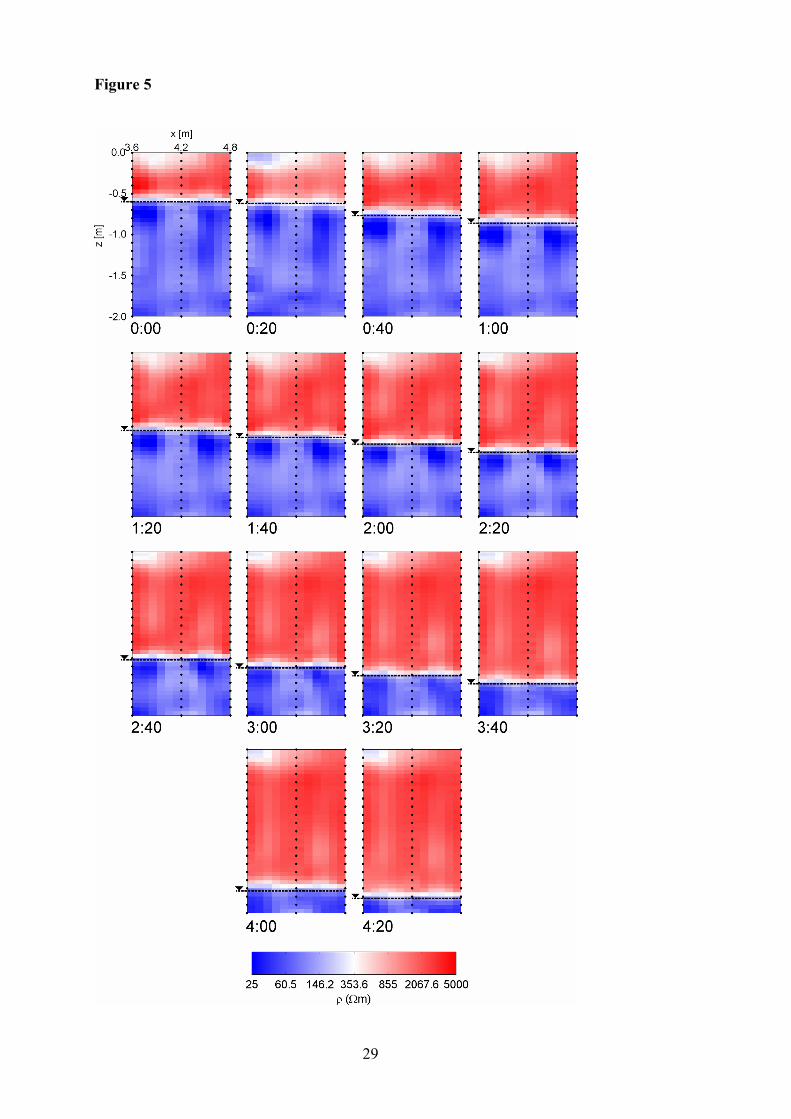
A sequence of inverted resistivity images for the full pumping cycle is presented in Figure 5.

Only the abstraction phase is shown, in which the water table falls from its maximum to its

minimum level. The 63 electrode positions used for the experiment are superimposed on the

images. The times shown refer to the elapsed time in hours/minutes relative to the beginning

of the experiment. Iteration 5 is shown for each inverted model, with RMS misfit errors

ranging between 3 and 8% throughout the sequence. In most of the images, the transition zone

spans one or two rows of model cells, corresponding to a maximum thickness of around

10 cm. This result suggests that the extent of the capillary fringe in Cell 1 is limited, which

13

confirms the relatively free-draining characteristics of the Chelford 16/30 sand discussed in

Section 3.2.1.

Averaging over a large number of model cells allows the calculation of representative values

for the bulk resistivities of (1) tap-water saturated and (2) partially saturated or dry sand in the

test cell. For the dataset obtained after 1:40 h, the water table divides the model

approximately in half. At that stage, the upper half of the cells has an average value of

~1,802 Ωm, the lower half of ~89 Ωm, i.e. the resistivity contrast between phreatic and

vadose zones is approximately 1:20. The fluid conductivity of the tap water was measured

with a hand-held conductivity meter and showed average values of 650–700 μS/cm. This

corresponds to fluid resistivities of 14.3–15.4 Ωm.

Conventionally measured water table data have been superimposed on the resistivity images

in Figure 5 as dashed lines. The sequence of images demonstrates that the ALERT

methodology is able to track the falling water table with great accuracy (within the limits of

the model discretisation). We found that, for each image in the sequence, the measured water

table coincides with the lower edge of the transition zone observed by ERT.

3.3 Experiment 2: monitoring lateral tracer migration

The second experiment was designed to extend the concepts established in Cell 1 to a more

complex imaging scenario. Multiple observation wells in Cell 2 were considered for imaging

lateral tracer migration using a 2D fence and a 3D grid. In addition to observing tracer

evolution with ALERT time-lapse imaging, conventional sampling was employed to facilitate

the comparison of direct measurements of fluid properties with results derived from electrical

imaging. A simple petrophysical relationship was used to convert bulk resistivities to

estimated fluid properties. The following description refers to representative experiments

carried out on 24 August 2006 (2D) and 13 September 2006 (3D).

3.3.1 Experimental setup, pumping regime and time scales

Prior to the start of the experiment, Cell 2 was filled with tap water to a level just below the

ground surface in order to pre-saturate the imaging zone and to flush out any potential

residuals from the pore spaces. Level sensors at the injection and abstraction ends of the cell

(Figure 2) were then set so that a constant head difference (and thus a constant hydraulic

gradient) of around 0.5 m (0.15 m bgl to 0.65 m bgl) was maintained across the cell

throughout the experiment. This resulted in an approximately uniform horizontal flow field in

the majority of the cell volume. The rate of flow was controlled by the hydraulic conductivity

14

of the Chelford 52 sand (saturated value 2.29×10-4 m/s) and the hydraulic gradient

(approximately 0.083) imposed by the pumping. With these values, horizontal flow rates

along Cell 2 of approximately 4–5 m/d were expected. Tracer movement at this rate was

deemed to be suitably slow for monitoring with ALERT.

3.3.2 Acquisition strategy

ERT measurements were made on nine simulated wells aligned in a vertical plane along the

centre of Cell 2 (W2 to W10, cf. Figure 2). Consequently, the imaging zone now comprised

eight neighbouring inter-borehole panels, resulting in a total of 144 electrodes used for this

experiment. As in Cell 1, bipole-bipole configurations were used exclusively. A comparison

of strategies analogous to that described under Section 3.2.2 showed that in the case of Cell 2,

panel-by-panel data acquisition could help avoid horizontal distortion. As the aim of the

second experiment was to image lateral movement (as opposed to vertical movement in Cell

1), a panel-by-panel strategy was preferred on this occasion in order to minimise image skew.

Due to the larger number of electrodes, longer measurement times were required. We found

that schemes with approximately 1400 individual resistance measurements gave the best

results in the shortest possible time. Using identical source parameters as in Cell 1, these

schemes took approximately 35 min to complete on the nine-well fence. Data acquisition was

therefore scheduled every 40 min and automatically performed by the ALERT system.

Individual datasets were again transferred to the data management server for processing.

Datasets were screened for quality, and only moderate pre-processing was found to be

necessary. Typically around 94% of measurements were used for imaging. Datasets were

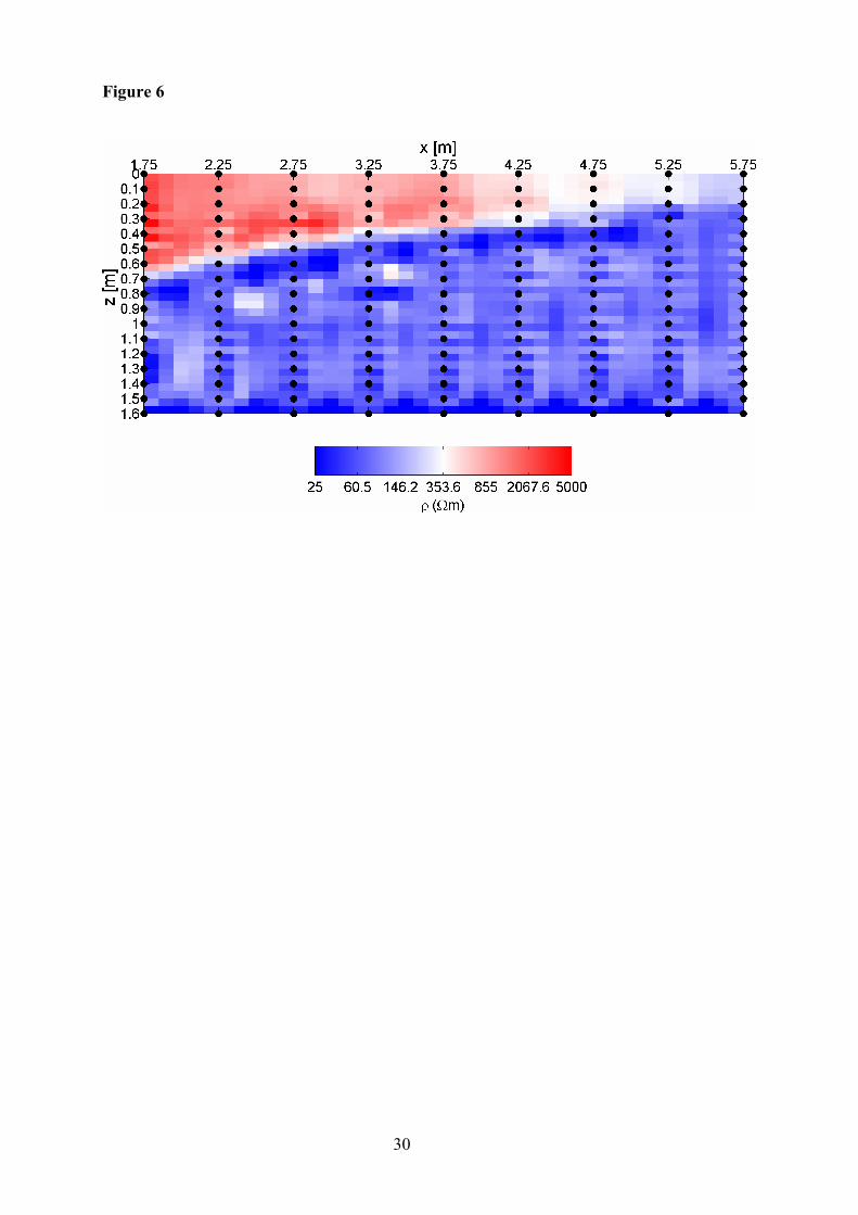
inverted in the same way as for Cell 1. A baseline image prior to tracer injection is shown in

Figure 6, proving that the phreatic surface of the stationary flow in Cell 2 follows a drawdown

curve caused by abstraction at the end of the cell.

3.3.3 Tracer design and injection procedure

Cooking salt (predominantly NaCl) dissolved in tap water at moderate concentrations is

environmentally benign and was considered suitable for use as a tracer fluid in our test cells.

The exact concentration is an important experimental design parameter as it controls not only

the electrical conductivity of the tracer (and hence the contrast against the background

medium), but also its density. As saline solution is denser than tap water, a saline plume

injected into a freshwater-saturated porous medium will sink under gravity. In the context of

our experiment, sufficiently high electrical contrast is desirable for successful resolution with

15

ERT, but high-concentration tracers may sink at a faster rate than the horizontal flow rate,

thus potentially missing the zone of greatest sensitivity.

Tracer design is discussed in some detail by Slater et al. [22], who point out that for a medium

saturated with a stagnant fluid of density ρ0, an estimate for the gravity-induced downward

flow of a plume of fluid of density ρ1 is described by

)( 01d ρρμ

−⋅

=gkv , (3)

where k denotes the intrinsic permeability of the medium, g the gravitational acceleration and

μ the fluid dynamic viscosity. The velocity vd is known as the Darcy velocity. A tracer

concentration of 20 g/l was adopted for this experiment, corresponding to an approximate

density contrast between tracer fluid and tap water of ≈20 kg/m3. Laboratory measurements

had established the saturated hydraulic conductivity of the Chelford 52 sand to be 2.29×10-4

m/s, corresponding to an intrinsic permeability of 2.34×10-11 m2 (≈24 darcy). Expected Darcy

velocities were therefore of the order of 0.4 m/day. Compared to the expected horizontal flow

rates along Cell 2 of approximately 4–5 m/d, gravitational sinking of the tracer fluid was

likely to be sufficiently slow to allow successful traversing of the imaging zone within the

time scale of the experiment. Our tracer fluid showed a fluid conductivity of 30 mS/cm

(corresponding to a resistivity of 0.33 Ωm), which is at least 40 times that of the tap water

used (average conductivity 650–700 μS/cm), thus offering good electrical contrast. A total of

25 l of tracer fluid was injected over a 1.5 h period through a multilevel sampler tube at W9 at

a depth of 0.4 m, so that the tracer was immediately exposed to the surrounding flow field.

3.3.4 Direct sampling strategy and comparison of properties

Pore water samples were obtained from Cell 2 at regular intervals during the tracer

experiment, so that direct comparison was possible between fluid properties determined on

the sample and those inferred from the electrical images. Using the multilevel sampler tubes

and a peristaltic pump, small samples (~30 ml) were extracted on several wells from a range

of depths at regular intervals coincident with electrical data acquisition. Fluid conductivities

were measured with a handheld conductivity meter.

Alternatively, fluid conductivities can be estimated from the bulk resistivities determined by

ERT through application of petrophysical relationships. In our experimental setup, only clean

unconsolidated sand is employed, which has a clay content of practically zero. It is therefore

safe to assume that surface conduction is negligible and simple estimates of fluid properties

16

can be made by applying Archie’s Law, in which fluid conductivity σw is linked to bulk

formation conductivity σt by an empirical formation factor [1]:

FS wnw

mwt σφσσ == (4)

In our experiments, this formation factor F can be estimated from the observed bulk

resistivity of tap-water-saturated sand, given that the pore water properties are well known.

This bulk value was calculated as a resistivity average for the phreatic zone as detected in the

baseline image (Figure 6), and an approximate formation factor of F≈5.9 was obtained by

calculating the ratio wt σσ .

3.3.5 Results and discussion

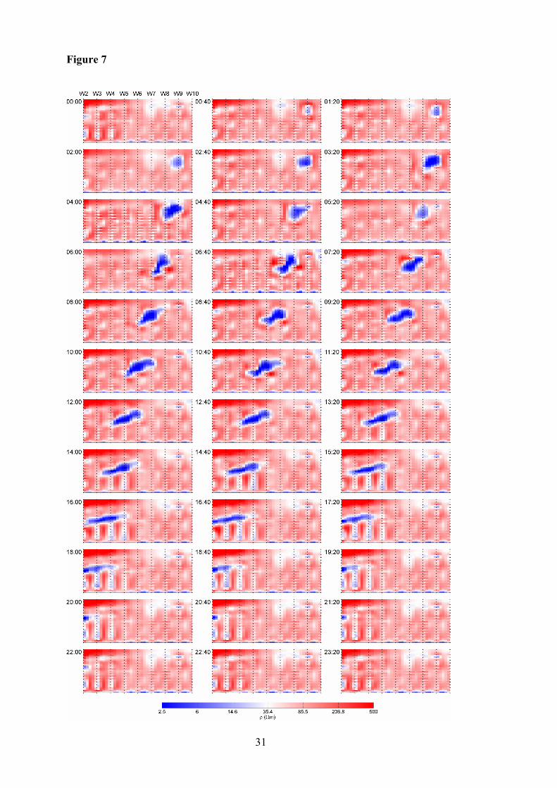
The sequence of inverted resistivity images obtained during the tracer test is shown in Figure

7. The time span required for the tracer to enter at the injection point, traverse the length of

the imaging zone and disappear from the images is approximately 24 hours. Given a

minimum interval of 40 min required per imaging snapshot (see Section 3.3.2), a maximum

number of 36 frames could be obtained over that period, highlighting the limitations in

temporal resolution currently achievable with ERT monitoring. Each tomogram covers the

full imaging zone comprising eight inter-borehole panels (W2–3 to W9–10, cf. Figure 2). The

simulated wells with the 144 electrode positions used for this experiment are superimposed on

the first image in Figure 7. The times shown refer to the elapsed time in hours/minutes

relative to the beginning of the experiment. The resistivity colour scale ranges from 2.5 Ωm

(blue) to around 390 Ωm (red), with intermediate resistivities (~19–50 Ωm) displayed as

transitionary colours. The chosen model discretisation contains 1280 model cells in 32 layers

(5 cm thickness) and 40 columns (10 cm width). Iteration 5 is shown for each inverted model,

with RMS errors reaching around 4–6% throughout the sequence.

In addition to the water-saturated zone and the dry or partially saturated zone already evident

from the baseline image (Figure 6), the tracer plume can now be clearly distinguished in the

images. As before, resistivities <20 Ωm are found to represent saturated sand with elevated

salinities. The lowest bulk resistivities observed are around 1.3 Ωm, i.e. over five times the

value of the tracer liquid at its original concentration. The first image in the sequence

coincides with the start of tracer injection, showing a faint conductive spot at the injection

point. The overall duration of tracer injection was approximately 1:30 h, hence injection was

completed within the first three image frames. In the following images, the conductive plume

then grows in size and can eventually be seen to move in the direction of the hydraulic

gradient (towards the left of the image) after 2:40 h. The neighbouring borehole is reached

17

after 3:20 h and parts of the plume begin to differentially move downwards under the

influence of gravitational sinking. This is particularly evident from 6:00 h onwards. In the

following images, the tracer plume assumes an increasingly elongated shape until its front

reaches the downstream boundary of the imaging zone. In the wake of the plume, the

saturated zone is found to quickly revert back to resistivity values comparable to those prior

to injection. The plume has almost completely disappeared from the imaging zone after

around 22:00 h. A downward loss of small amounts of tracer in the leftmost four wells (W2 to

W5) is revealed in the images, manifested in increased conductivities along the borehole

columns. This can be explained by the fact that W2 to W5 were amongst a group of wells that

had been completed with slotted casing, thereby allowing the passing tracer front to penetrate

the free water column inside the well.

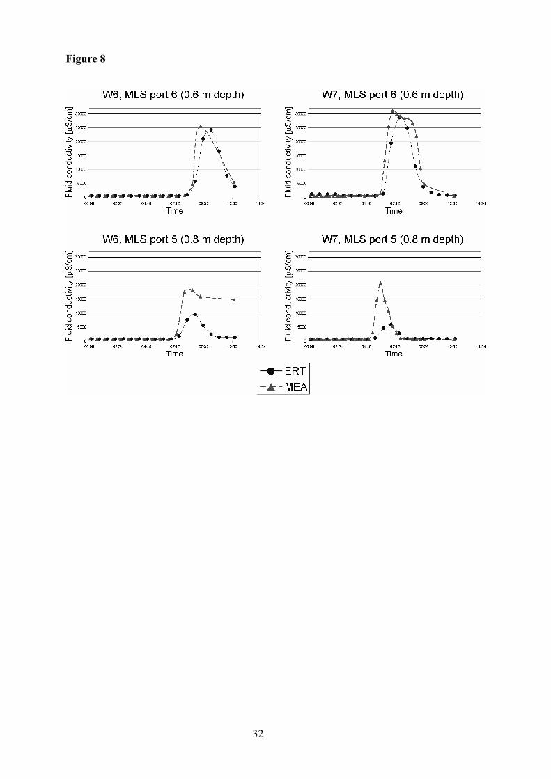
A time-sequence of ERT images can act as a proxy for spatio-temporal sampling of tracer

breakthrough [4]. For the purpose of comparison with the pore water samples, fluid

conductivity estimates were obtained from the ERT results. Bulk resistivities were extracted

from ERT model cells that corresponded to the locations at which direct samples had been

obtained from MLS ports. By applying the empirically determined formation factor described

in Section 3.3.4, fluid conductivities were estimated. Plotting both datasets along the same

time axis (“breakthrough curves”) allowed us to study the evolution of pore water

conductivity as seen by the two different methodologies. The results of this comparison are

shown in Figure 8. Both datasets show characteristic maxima at times when the tracer plume

passes the sampling point. We observed excellent correspondence between both

methodologies at the shallower sampling points. At greater depth however, the ERT-derived

estimates are consistently lower than those obtained from direct sampling. We suspect that

this may be either (1) an intrinsic effect of the smoothness constrained inversion algorithm or

(2) a systematic error introduced by the physical sampling procedure, which may disturb the

local flow regime by abstracting significant amounts of pore fluid. This effect is exacerbated

at greater depths, where more vigorous pumping over longer periods of time is usually

required to extract a viable pore water sample.

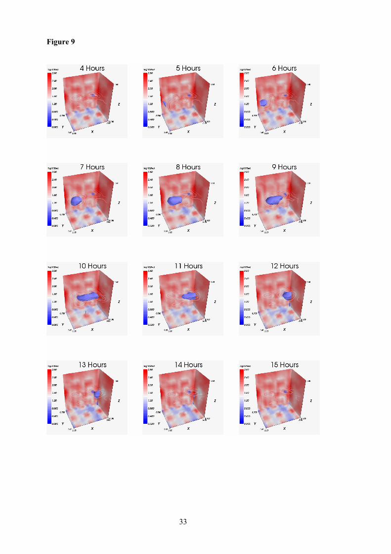
3.4 The 3D experiment: setup, results and discussion

An identical tracer experiment to the one described in Section 3.3 was carried out to

demonstrate the viability of 3D crosshole monitoring with ALERT. Due to the conceptual

similarity, we only briefly describe the setup of the 3D experiment here. A 3×3 grid of

simulated wells in Cell 2 (W13, 14, 15, 4, 5, 6, 17, 18, 19, cf. Figure 2) was used to acquire

18

3D imaging data at regular intervals (one frame per hour). For each 3D frame, a total number

of 2112 resistance measurements were made across all possible combinations of inter-

borehole panels between neighbouring wells on the 3×3 grid (e.g. W13–4, W13–14), but no

diagonal panels (e.g. W13–5) were included. Typically, around 95% of these measurements

were used for inversion. A 3D least-squares smoothness-constrained algorithm was employed

(Res3dinv, [18]).

Saline tracer with the same specifications as for the 2D case was injected through W7. The

greater proximity of the injection point to the imaging zone was expected to result in the

plume geometry to remain more coherent whilst passing through the monitored volume. The

setup also implies a shorter time scale of the 3D experiment compared to the 2D scenario. The

results of this experiment are shown in Figure 9 as a sequence of 3D tomograms (image

cubes) centred on the 3×3 grid. The orientation of the coordinate system is such that the x-axis

is parallel to the long side of Cell 2, with numbers increasing from the abstraction end

towards the injection end of the cell. The flow field therefore enters the imaging cubes from

the left and exits on the right through the back wall of the cube. Resistivity isosurfaces with a

5 Ωm threshold value have been calculated for each frame, reflecting the approximate volume

within which the tracer plume is contained at that particular time. The first arrival of the tracer

plume at the imaging zone is observed after five hours. The plume then traverses the

monitored volume over a period of several hours. It is well constrained within the 3D volume

despite the relatively small number of sensors available for this experiment. After 14 hours

the plume has left the imaging zone and no residual trace is visible after that time.

4 Conclusions

We have developed the technologies and procedures required to implement the ALERT

concept of automated near-real-time geoelectrical monitoring, allowing us to remotely

initiate, control and manipulate data acquisition and processing for time-lapse electrical

imaging and tomographic reconstruction. Validation of this concept has been achieved

through a series of controlled hydraulic experiments using cross-borehole ERT

measurements. We have successfully demonstrated that ALERT is capable of monitoring

generic hydraulic processes of varying complexity (2D plus time, 3D plus time) and at

relatively short timescales, which are often associated with safety-critical applications (e.g.

monitoring of embankment dams, subsurface reservoirs or hydrothermal systems) or

commercial/industrial operations (e.g. leachate recirculation in landfills, underground gas

storage facilities). The limiting factor inherent to the ALERT concept is the finite amount of

19

time needed to acquire sufficiently comprehensive datasets, thus allowing reliable

tomographic reconstruction. Our experiments have shown that typical frame rates of 1.5–3

images per hour are possible without compromising image quality or jeopardising the flow of

information to and from the remote site.

We have investigated different strategies for practical data acquisition with the aim of

harmonising the measurement scheme with the characteristics of the monitored process. For

crosshole data acquisition in multi-well monitoring applications, the interleaved measurement

sequence favours hydraulic processes with rapidly occurring changes in vertical direction and

can therefore be regarded as an optimised strategy for level monitoring applications. The

panel-by-panel strategy was found to favour processes causing rapid horizontal changes, and

is therefore optimal for flow monitoring.

A simple quantitative comparison between ERT-derived pore water properties and direct

sampling results showed good correspondence in the observed breakthrough curves,

indicating that the ALERT concept holds promise beyond the purely qualitative interpretation

of time-lapse images. Future developments should focus on the potential for shortening

measurement times and optimising acquisition schemes in order to further improve the value

of ALERT in realistic field applications.

5 Acknowledgements

This paper is published with the permission of the Executive Director of the British

Geological Survey (NERC). We gratefully acknowledge the contributions made by many of

our BGS colleagues. We thank Philip Carpenter, Solenne Grellier, Ghislain de Marsily and an

anonymous reviewer for their thorough reviews and constructive comments, which have

helped us improve this manuscript. The French translations were kindly provided by Ghislain

de Marsily. Our research was funded by the Veolia Environmental Trust (project

RES/C/6034) and English Partnerships under the terms of the UK Landfill Tax Regulations

1996.

20

6 References

[1] G.E. Archie, The electrical resistivity log as an aid in determining some reservoir

characteristics, Trans. Am. Inst. Min. Metall. Pet. Eng. 146 (1942) 54-62.

[2] M. Bano, Effects of the transition zone above a water table on the reflection of GPR

waves (DOI 10.1029/2006GL026158), Geophysical Research Letters 33 (2006) L13309.

[3] A. Binley, G. Cassiani, R. Middleton, P. Winship, Vadose zone flow model

parameterisation using cross-borehole radar and resistivity imaging, Journal of Hydrology

267 (2002) 147-159.

[4] A. Binley, S. Henry-Poulter, B. Shaw, Examination of solute transport in an

undisturbed soil column using electrical resistance tomography, Water Resources Research 32

(1996) 763-769.

[5] J.E. Chambers, O. Kuras, P.I. Meldrum, R.D. Ogilvy, Comparison of fundamental

modes of illumination for cross-hole electrical impedance tomography: part I - sensitivity

analysis, 9th Meeting of the Environmental and Engineering Geophysical Society - European

Section, Prague, 2003.

[6] J.A. Cherry, R.W. Gillham, E.G. Anderson, P.E. Johnson, Migration of Contaminants

in Groundwater at a Landfill: A Case Study, 2. Groundwater Monitoring Devices, Journal of

Hydrology 63 (1983) 31-49.

[7] W. Daily, A. Ramirez, R. Newmark, K. Masica, Low-cost reservoir tomographs of

electrical resistivity, The Leading Edge 23 (2004) 472-480.

[8] R.A. Freeze, J.A. Cherry, Groundwater, Prentice Hall, 1979.

[9] H. French, A. Binley, Snowmelt infiltration: monitoring temporal and spatial

variability using time-lapse electrical resistivity, Journal of Hydrology 297 (2004) 174-186.

[10] S. Grellier, R. Guerin, H. Robain, A. Bobachev, F. Vermeersch, A. Tabbagh,

Monitoring of Leachate Recirculation in a Bioreactor Landfill by 2-D Electrical Resistivity

Imaging, Journal of Environmental and Engineering Geophysics 13 (2008) 351-360.

[11] R. Guerin, M.L. Munoz, C. Aran, C. Laperrelle, M. Hidra, E. Drouart, S. Grellier,

Leachate recirculation: moisture content assessment by means of a geophysical technique,

Waste Management 24 (2004) 785-794.

[12] P.R.N. Hobbs, J.R. Hallam, A. Forster, D.C. Entwisle, L.D. Jones, A.C. Cripps, K.J.

Northmore, S.J. Self, J.L. Meakin, Engineering geology of British rocks and soils: Mudstones

of the Mercia Mudstone Group. Research Report RR/01/02, British Geological Survey, 2002.

21

[13] S. Johansson, T. Dahlin, Seepage monitoring in an earth embankment dam by repeated

resistivity measurements, European Journal of Engineering and Environmental Geophysics 1

(1996) 229-247.

[14] A. Kemna, B. Kulessa, H. Vereecken, Imaging and characterisation of subsurface

solute transport using electrical resistivity tomography (ERT) and equivalent transport

models, Journal of Hydrology 267 (2002) 125-146.

[15] O. Kuras, J.E. Chambers, P.I. Meldrum, R.D. Ogilvy, Comparison of fundamental

modes of illumination for cross-hole electrical impedance tomography: part II - synthetic

modelling, 9th Meeting of the Environmental and Engineering Geophysical Society -

European Section, Prague, 2003.

[16] D.J. LaBrecque, G. Heath, R. Sharpe, R. Versteeg, Autonomous Monitoring of Fluid

Movement Using 3-D Electrical Resistivity Tomography, Journal of Environmental and

Engineering Geophysics 9 (2004) 167-176.

[17] M.H. Loke, R.D. Barker, Least-squares deconvolution of apparent resistivity

pseudosections, Geophysics 60 (1995) 1682-1690.

[18] M.H. Loke, R.D. Barker, Practical techniques for 3D resistivity surveys and data

inversion, Geophysical Prospecting 44 (1996) 499-523.

[19] R.D. Ogilvy, O. Kuras, P.I. Meldrum, P.B. Wilkinson, J. Gisbert, S. Jorreto, A. Pulido

Bosch, A. Kemna, F. Nguyen, P. Tsourlos, Automated monitoring of coastal aquifers with

electrical resistivity tomography, in: A. Pulido Bosch, J.A. López-Geta, G. Ramos González

(Eds.), Coastal Aquifers: Challenges and Solutions, Instituto Geológico y Minero de España,

Madrid, 2007, pp. 333-342.

[20] G.A. Oldenborger, M.D. Knoll, P.S. Routh, D.J. LaBrecque, Time-lapse ERT

monitoring of an injection/withdrawal experiment in a shallow unconfined aquifer,

Geophysics 72 (2007) F177-F188.

[21] P. Sjödahl, T. Dahlin, S. Johansson, Detection of Internal Erosion and Seepage Using

Resistivity Monitoring, WasserWirtschaft 10 (2007) 54-56.

[22] L. Slater, A.M. Binley, W. Daily, R. Johnson, Cross-hole electrical imaging of a

controlled saline tracer injection, Journal of Applied Geophysics 44 (2000) 85-102.

[23] L.D. Slater, S.K. Sandberg, Resistivity and induced polarization monitoring of salt

transport under natural hydraulic gradients, Geophysics 65 (2000) 408-420.

[24] P. Stummer, H. Maurer, A.G. Green, Experimental design: Electrical resistivity data

sets that provide optimum subsurface information, Geophysics 69 (2004) 120-139.

22

[25] R. Versteeg, M. Ankeny, J. Harbour, G. Heath, K. Kostelnik, E. Mattson, K. Moor, A.

Richardson, K. Wangerud, A structured approach to the use of near-surface geophysics in

long-term monitoring, The Leading Edge 23 (2004) 700-703.

[26] E.W. Washburn, The Dynamics of Capillary Flow, Physical Review 17 (1921) 273.

[27] P.B. Wilkinson, J.E. Chambers, P.I. Meldrum, R.D. Ogilvy, S. Caunt, Optimization of

Array Configurations and Panel Combinations for the Detection and Imaging of Abandoned

Mineshafts using 3D Cross-Hole Electrical Resistivity Tomography, Journal of

Environmental and Engineering Geophysics 11 (2006) 213-221.

[28] P.B. Wilkinson, P.I. Meldrum, J.E. Chambers, O. Kuras, R.D. Ogilvy, Improved

strategies for the automatic selection of optimized sets of electrical resistivity tomography

measurement configurations, Geophysical Journal International 167 (2006) 1119-1126.

[29] B.V. Zhmud, F. Tiberg, K. Hallstensson, Dynamics of Capillary Rise, Journal of

Colloid and Interface Science 228 (2000) 263-269.

[30] B. Zhou, S.A. Greenhalgh, Cross-hole resistivity tomography using different electrode

configurations, Geophysical Prospecting 48 (2000) 887-912.

23

7 Figures

Figure 1:

Layout of Cell 1. (a) Plan view; (b) cross-sectional view.

Configuration de la Cellule 1. (a) Vue en plan; (b) vue en coupe.

Figure 2:

Layout of Cell 2. (a) Plan view; (b) cross-sectional view; (c) flow field and tracer injection.

Configuration de la Cellule 2. (a) Vue en plan; (b) vue en coupe; (c) champ d’écoulement et

point d’injection du traceur.

Figure 3:

Cross-borehole measurement configurations and data acquisition strategies. (a) The two

fundamental sets of potential measurements per current injection employed in our

experiments (C1, C2 = current electrodes; P1, P2 = potential electrodes). The set of

measurements on the left-hand side is always carried out first, followed by the set on the

right-hand side. (b) Panel-by-panel strategy; (c) interleaved strategy.

Configuration des mesures entre forages et stratégies d’acquisition des données. (a) Les deux

ensembles fondamentaux des mesures de potentiel pour chaque injection de courant mis en

œuvre dans l’expérience (C1, C2 = électrodes d’envoi de courant, P1, P2 électrodes de

mesure de potentiel). L’ensemble des mesures sur le côté gauche est toujours fait en premier,

suivi par l’ensemble sur le côté droit. (b) Stratégie panneau par panneau; (c) stratégie par

couches.

Figure 4:

Comparison of data acquisition strategies for Cell 1 during pumping (falling water level). (a)

Panel-by-panel strategy; (b) interleaved strategy.

Comparaison des stratégies d’acquisition de données pour la Cellule 1 pendant le pompage

(niveaux d’eau descendants). (a) Stratégie panneau par panneau; (b) stratégie par couches.

Figure 5:

Sequence of images for Cell 1 during a period of falling water levels. Conventionally

measured levels are superimposed as dashed lines.

24

Suite d’images pour le Cellule 1 pendant une période de descente des niveaux d’eau. Les

mesures conventionnelles de niveaux sont ajoutées en traits tiretés.

Figure 6:

Baseline image of Cell 2 prior to tracer injection (Iteration 5, RMS error 5.9%). The colour

scale employed differentiates between the phreatic and vadose zones.

Image de base de la Cellule 2 avant l’injection du traceur (Itération 5, racine carrée de l’erreur

quadratique moyenne de 5,9%). L’échelle de couleur différencie la zone phréatique saturée et

la zone vadose non saturée.

Figure 7:

Results of the experiment to examine lateral tracer movement showing a sequence of inverted

resistivity images during tracer injection into Cell 2.

Résultats de l’expérience pour examiner la migration latérale du traceur, montrant une suite

d’images de résistivités inversées pendant l’injection du traceur dans la Cellule 2.

Figure 8:

Comparison of breakthrough curves obtained from ALERT images (ERT) and direct

sampling (MEA).

Comparaison des courbes de restitution du traceur obtenues par les images ALERT (ERT) et

par échantillonnage direct (MEA).

Figure 9:

Results of the 3D experiment to examine lateral tracer movement.

Résultats de l’expérience 3D pour étudier la migration latérale du traceur.

25

Figure 1

26

Figure 2

27

Figure 3

28

Figure 4

29

Figure 5

30

Figure 6

31

Figure 7

32

Figure 8

33

Figure 9