3. A SUCCESSIVE LINEAR ESTIMATOR FOR ELECTRICALRESISTIVITY TOMOGRAPHY

Tian-Chyi J. Yeh, Junfeng Zhu, Andreas Englert, Amado Guzman,and Steve Flaherty

3.1. Introduction

A dc resistivity survey is an inexpensive and widely used technique for inves-tigation of near surface resistivity anomalies. It recently has become popularfor the investigation of subsurface pollution problems (NRC, 2000). In prin-ciple, it measures the electric potential field generated by a transmission of dcelectric current between electrodes implanted at the ground surface. Then, anapparent (bulk or effective) electrical resistivity for a particular set of mea-surement electrodes is calculated using formulas that assume homogeneousearth. Many pairs of current transmission and electric potential measurementsare used to “map” subsurface electrical resistivity anomalies.

This conventional resistivity survey is analogous to classical aquifer testin which an aquifer is excited by pumping at one well and the response ofthe aquifer (e.g. drawdown-time relation or well hydrograph) is observed atanother well. The theoretical well hydrograph from an analytical solution thatassumes aquifer homogeneity and infinite domain (e.g. Theis’ solution, 1935)is then used to match the observed hydrograph to obtain apparent or effectiveaquifer transmissivity and storage coefficient. Due to the homogeneity as-sumption, the theoretical drawdown represents a spatially averaged drawdownin a heterogeneous aquifer. This average drawdown is unequivocally differentfrom the one observed at a well in a heterogeneous aquifer, although the differ-ence may be small due to diffusive nature of the flow process. Thus, applyingTheis’ solution to aquifer tests in a heterogeneous aquifer is tantamount tocomparing apples to oranges (Wu et al., 2005). They suggested that the appar-ent transmissivity represents a weighted average of transmissivity anomaliesover the cone of depression. High weights are given to transmissivity anoma-lies near the observation and the pumping well. The apparent transmissivityreflects, as a consequence, local geology but it can also be affected by signif-icant geologic anomalies within the cone of depression. In other words, thephysical meaning of the apparent transmissivity can be highly dubious.

The strong similarity between traditional aquifer and apparent resistivityanalysis leads us to conclude that conventional analysis of electrical resistivity

H. Vereecken et al. (eds.), Applied Hydrogeophysics, 45–74.C© 2006 Springer.

45

46 TIAN-CHYI J. YEH ET AL.

survey is another example of comparison between apples and oranges. Infact, the apparent resistivity approach has been found virtually ineffective forenvironmental applications, where electrical resistivity anomalies are subtle,complex, and multi-scale (Yeh et al., 2002).

Meanwhile, a contemporary electrical resistivity survey (electrical resis-tivity tomography, ERT) has been designed to collect extensive electric currentand electric potential data sets in multi-dimensions. The resistivity field is es-timated from the inversion of the data set using, a mathematical computermodel based on a regularized optimization approach and without the assump-tion of subsurface homogeneity (e.g. Daily et al., 1992; Ellis and Oldenburg,1994; Li and Oldenburg, 1994; and Zhang et al., 1995). However, the gen-eral uniqueness and resolution of the three-dimensional electrical resistivityinversion have not been investigated sufficiently thus far (NRC, 2000).

While the physical process is different between electric current andgroundwater flow, the governing equation for electric current and potentialfield created by an electrical resistivity survey is similar to that for steady flowin saturated porous media induced by pumping or injection. The mathemati-cal inversion of an electrical resistivity survey is thus analogous to that of agroundwater aquifer test. Groundwater hydrologists and reservoir engineershave attempted to solve the inverse problem of flow through multidimen-sional, heterogeneous porous media for the last few decades (e.g. Gavalaset al., 1976). Reviews of the inverse problem of subsurface hydrology andvarious solution techniques can be found in Yeh (1986), Sun (1994), andMcLaughlin and Townley (1996). The general consensus is that prior infor-mation on geological structure, and some point measurements of parametersto be estimated are necessary to better constrain solution of the inverse prob-lem. A similar finding was also reported by Oldenburg and Li (1999) and Liand Oldenburg (2000) for the inverse problems in geophysics.

A multi-variate linear estimator (cokriging) has been widely used bygroundwater hydrologists to estimate the hydraulic conductivity field fromscattered measurements of pressure head and hydraulic conductivity inaquifers (e.g. Kitanidis and Vomvoris, 1983; Hoeksema and Kitanidis, 1984;Yeh and Zhang, 1996). The popularity of cokriging is attributed to its abilityto incorporate spatial statistics, point measurements of hydraulic conductivityand hydraulic head into the estimation, and its ability to yield conditional meanestimates. Cokriging is also known for its ability to quantify the uncertaintyassociated with its estimate due to limited information and heterogeneity.Kitanidis (1997) discussed the differences between cokriging and classicalinverse methods in subsurface hydrology and showed cokriging is a Bayesianformalism. Nevertheless, cokriging is a linear estimator and it is limited tomildly nonlinear systems, such as aquifers of mild heterogeneity, where thevariance of the natural logarithm of hydraulic conductivity, σ 2

lnK, is less than

SUCCESSIVE LINEAR ESTIMATOR 47

0.1. When the degree of aquifer heterogeneity is large (σ 2lnK > 1), the linear

assumption becomes inadequate and cokriging cannot take full advantage ofthe hydraulic head information (Yeh et al., 1996).

To overcome this shortcoming, Yeh et al. (1995, 1996), Gutjahr et al.(1994), and Zhang and Yeh (1997) developed an iterative geostatistical tech-nique, referred to as a successive linear estimator (SLE). This technique usesa linear estimator successively to incorporate the nonlinear relation betweenhydraulic properties and the hydraulic head in inverse modeling. It also suc-cessively updates conditional covariances to quantify reductions in uncer-tainty due to successive improvements of the estimate. Yeh et al. (1995 and1996), and Zhang and Yeh (1997) demonstrated that using the same amountof information, SLE revealed a more detailed hydraulic conductivity fieldthan cokriging. Hughson and Yeh (2000) successfully applied SLE to the in-verse problem in three-dimensional, variably saturated, heterogeneous porousmedia.

Based on the SLE algorithm, Yeh and Liu (2000) developed a sequentialsuccessive linear estimator (SSLE) to process the large amount of data sets cre-ated by steady-state hydraulic tomography for imaging aquifer heterogeneity.In addition, they investigated effects of monitoring intervals, pumping inter-vals, and the number of pumping locations on the final estimate of hydraulicconductivity. Subsequently, guidelines for design of hydraulic tomographytests were established, which are also applicable to ERT. The SSLE algorithmfor hydraulic tomography was subsequently validated by Liu et al. (2002) usingsandbox experiments. Robustness of SSLE compelled Zhu and Yeh (2005) todevelop three-dimensional (3-D) transient hydraulic tomography, which canbe used to image 3-D hydraulic conductivity and the specific storage fields inheterogeneous aquifers.

Successes of SSLE for hydraulic tomography have motivated its appli-cation to ERT. In particular, Yeh et al. (2002) developed a SSLE algorithmfor ERT and investigated the effectiveness of surface and downhole electrodearrays in stratified geological media. They concluded that surface electrodearrays detect only anomalies near the surface and downhole arrays providemore accurate mapping of the anomalies at great depths. More importantly,using field core samples Baker (2001) and Yeh et al. (2002) investigatedthe spatial variability of Archie’s law that relates moisture content to elec-trical resistivity. Significant spatial variability of the parameters of the lawwas found in a 20 m × 20 m × 15 m vadose zone in an alluvium deposit.Thereafter, numerical experiments were undertaken to demonstrate effects ofthe variability on ERT estimation of moisture content in the vadose zone.Finally, they cautioned interpretation of ERT for mapping changes in mois-ture content in the vadose zone if the variability of Archie’s parameter isignored.

48 TIAN-CHYI J. YEH ET AL.

To resolve the variability problem, Liu and Yeh (2004) developed an in-tegrative ERT inversion approach based on SSLE. This integrative approachallows inclusion of prior knowledge of spatial statistics of the parameters ofArchie’s law and the resistivity field to be estimated as well as direct mea-surements of the parameters, resistivity, and moisture content values. Theydemonstrated how the new approach can be used to determine moisture con-tent distribution directly without using time-lapse ERT surveys.

Since SSLE, a geostatistically based inverse model, is relatively new ingeophysics, the aim of this chapter is to introduce the SSLE algorithm for ERTand to demonstrate its usefulness. Specifically, we first discuss in Section 3.2the basic concept of stochastic representation of ERT inverse problems andthen explain why the analysis of ERT survey should be viewed as a conditionalmean estimation of a spatially stochastic resistivity field. In Section 3.3, themathematical formulation of SSLE for ERT inversion is presented. Next, nu-merical examples are used to illustrate the robustness of the algorithm and theconcept of ERT (namely, an intelligent data collection scheme to resolve theill-poseness of electrical resistivity inversion problem) in Section 3.4. Exam-ples of applications of ERT to monitoring solute distributions in aquifers andmoisture content distributions in the vadose zone then follow. Using theseexamples, we show effects on the quality of ERT inversion by condition-ing with direct measurements of concentration and moisture content. Lastly,the application of the SSLE algorithm to an ERT survey in a mine leachingfield is presented (Section 3.5), where a stochastic approach for eliminat-ing biased and noisy ERT data – an important step in ERT analysis – ispresented.

3.2. Stochastic Conceptualization of ERT Inverse Problems

Assume that in a geological formation, the electric current flow induced byan electrical resistivity survey can be described by

∇ · [ξ (x) ∇φ(x)] + I (x) = 0 (1)

where x is the location vector (x, y, z), φ is the electric potential [V], I (x)represents the electric current source per volume [A/m3], and ξ is the electricalconductivity [S/m] within a previously defined volume, a reciprocal of theelectrical resistivity, ρ[ohm-m], which is assumed to be locally isotropic. Theboundary conditions associated with Equation (1) are

φ|G1= φ∗ and ξ (x) ∇φ · n|G2

= q (2)

where φ∗ is the electric potential specified at boundary G1, q denotes the

SUCCESSIVE LINEAR ESTIMATOR 49

prescribed electric current per unit area (current density), and n is the unitvector normal to the boundary G2.

The electrical conductivity or resistivity of geologic media varies spatiallydue to inherent heterogeneous geologic processes (Sharma, 1997). One wayto describe the spatial variability of electrical conductivity is the stochasticrepresentation approach, similar to that used in geohydrology for the variabil-ity of hydraulic properties of aquifers and vadose zones (see Gelhar, 1993;Yeh, 1992, 1998). Specifically, the electrical conductivity field of a geologicformation is considered as a stochastic process, ξ (x, π ), where π is the en-semble index, ranging from one to infinity. That is, the value of ξ (x) at eachlocation x in the formation is a random variable regardless if the value isknown or unknown. The electrical conductivity field of the formation, there-fore, is visualized as a collection of an infinite number of random variablesin space. This stochastic process can be described by a mean, 〈ξ (x)〉 = �

(where 〈 〉 denotes the expected value, i.e., ensemble average or the averageover the infinite number of possible realizations or π in ensemble space) andperturbations around the mean, ω(x, π ), characterized by a joint probabilitydistribution. For simplicity, the ensemble index, π , will be dropped hereafter.

Assuming that the perturbation is a second-order stationary stochasticprocess (that is, the stochastic process has a stationary mean and varianceas well as its covariance depends on the separation distance only), its jointprobability distribution can thus be adequately represented by its mean andcovariance function, Rωω(η), where η is the separation vector between elec-trical conductivity values at two locations. The covariance function representsin a statistical sense the spatial correlation structure (pattern) of the electricalconductivity of a geologic formation. More specifically, the spatial correlationstructure states the likelihood of occurrence of the same electrical conductiv-ity value at two different locations. Because of this stochastic representationof the electrical conductivity, the electric potential field induced during anelectrical resistivity survey can also be considered as a stochastic process. Itcan be described by φ(x) = V (x) + v(x), where V (x) = 〈φ(x)〉 and v(x) isthe perturbation of the electric potential.

Suppose that electrical conductivity measurements (referred to as the pri-mary variable or primary information), ξ ∗

i (where i = 1, . . . , n, and n is thetotal number of electrical conductivity measurements) are available from bore-hole electrical resistivity surveys. From these measurements, we have esti-mated the mean and covariance function of the electrical conductivity field ofthe geologic formation. Now, suppose that an ERT survey is then conducted.For each transmission of electric current during the survey, we have collectedk electric potential values, v∗

j , where j = n + 1, n + 2, . . . , n + k. Hereafter,the electric potential measurements are referred to as secondary information.Now, our goal is to exploit the primary and secondary information available

50 TIAN-CHYI J. YEH ET AL.

to estimate the electrical conductivity distribution over the volume of the ge-ologic formation. Mathematically, we are seeking an inverse model that canproduce the electric potential and electrical conductivity fields that satisfy thefollowing conditions. That is, they must preserve the observed electric po-tential and electrical conductivity values at sample locations and also satisfyunderlying physical processes (i.e., the governing electric potential equation).In a conditional probability context, such electric potential field and electricalconductivity field are conditional realizations of φ(x) and ξ (x) fields, respec-tively, among many possible realizations of the ensemble. In other words,they are a subset of the ensemble of each field, which meets the prescribedconditions.

These conditional realization of the electrical conductivity field can also beexpressed as the sum of the conditional mean electrical conductivity field andits conditional perturbation field, i.e., ξc(x) = �c(x) + ωc(x). The subscript cdenotes the state of being conditioned. Similarly, the conditional electric po-tential fields can be written as φc(x) = Vc(x) + vc(x). It should be noticed thatas more independent data or constrains are used to condition the stochasticprocesses, the processes should approach particular realizations of the pro-cesses (i.e., the reality). Transmission of electric current at different locationsand recording of electric potentials using the same sampling network (i.e.,a tomographic survey) as in an ERT survey is tantamount to creating manyindependent constraints to condition the stochastic processes. Nevertheless,many possible realizations of such conditional ξ (x) and φ(x) fields remain inspite of the tomographic survey. The means of these conditional fields (i.e.,conditional means of �c(x) and Vc(x)) on the other hand are unique, althoughnot necessarily reflective of the true fields.

One way to obtain these conditional mean fields is to solve the inverseproblem for all possible conditional realizations of the electrical resistivityfield. An average of all of the possible realizations then yields the conditionalmean electrical resistivity field (see Hanna and Yeh, 1998 and others forgeohydrology applications). An alternative approach is to solve the inverseproblem in terms of the conditional mean equation, as described below.

In order to formulate the conditional mean equation, we first substitutethe conditional stochastic variables into the governing electric potential Equa-tion (1) and then take the expected value of the resultant equation. Theconditional-mean equation thus takes the following form

∇ · [�c (x) ∇Vc (x)] + ∇ · 〈ωc (x) ∇vc (x)〉 + I (x) = 0 (3)

In Equation (3), the current source, I (x), is treated as a deterministic constantthat is known. According to Equation (3), the true conditional mean �c (x)and Vc (x) fields do not satisfy the continuity Equation (3) unless the secondterm involving the product of perturbations is zero. This term represents the

SUCCESSIVE LINEAR ESTIMATOR 51

uncertainty due to a lack of information of the two variables at locations wheremeasurements are not available. The uncertainty will vanish under two con-ditions, namely: 1) all the electrical conductivity values in the domain (i.e.,the geologic formation) are specified exactly (i.e., ωc (x) = 0); or 2) all theelectric potential values in the domain are known perfectly (i.e., vc (x) = 0) asare the electric fluxes at the boundaries. In practice, these two conditions willnever be met and evaluation of this term is intractable at this moment. Conse-quently, in the subsequent analysis we will assume this term is proportionalto the conditional mean electric potential gradient such that we can rewritethe mean equation as

∇ · [�ceff (x) ∇Vc (x)] + I (x) = 0 (4)

This conditional mean equation has the same form as Equation (1) butvariables are expressed as the conditional effective electrical conductivity,�ceff (x), and conditional mean electric potential field, Vc (x). The conditionaleffective electrical conductivity thus is a parameter field that combines the con-ditional mean electrical conductivity, �c (x), and 〈ωc (x) ∇vc (x)〉 (∇Vc(x))−1.According to this concept, the conditional effective electrical conductivityfield will agree with the electrical conductivity measurements at sample lo-cations. It yields a conditional mean electric potential field that preservesvalues of electric potential measurements when it is employed in the for-ward model, Equation (4), subject to the prescribed boundary conditions.Following this concept, an optimal inverse solution to Equation (4) seeks theconditional effective electrical conductivity field. The sequential successivelinear estimator (SSLE) approach to be introduced below is designed for thispurpose.

3.3. Sequential Successive Linear Estimator for ERT

Suppose that a geologic medium to be investigated is discretized into Melements and each element has an electrical conductivity value, ξ (x). Formathematical convenience, the natural logarithm of the electrical conductiv-ity, ln ξ (x), instead of ξ (x), will be used as the stochastic process for ouranalysis. That is, ln ξ (x) = F + f (x) and 〈ln ξ (x)〉 = F , which is assumed tobe spatially invariant (although it is not necessary). One of the advantagesof using ln ξ (x) is that this approach avoids negative value of estimated ξ (x)values during the inverse procedure.

To derive the conditional effective electrical conductivity that will producea conditional mean potential field in Equation (4), SSLE starts with the clas-sical cokriging technique to construct a cokriged, mean-removed log conduc-tivity field. The technique uses observed electrical conductivity perturbations,

52 TIAN-CHYI J. YEH ET AL.

f ∗i , and the observed electric potential perturbations, v∗

j , caused by one trans-mission of electric current during the tomography. That is,

f (x0) =n∑

i=1

λi0 f ∗ (xi ) +n+k∑

j=n+1

μ j0v∗ (

x j

)(5)

where ˆf (x0) is the cokriged f value at location, x0. Then, we defineYk(x0) = [F + f (x0)] and the cokriged electrical conductivity, ξk (x0), is givenas exp[Yk(x0)]. The cokriging weights, λi0 and μ j0, in Equation (5) representinfluences of observations, f ∗(xi ) and v∗(x j ), at locations xi and x j on the

estimate f (x0) at x0. They are evaluated from solving the following systemof equations

n∑

i=1

λio Rff (x, xi ) +n+k∑

j=n+1

μjo Rfv (x, x j )= Rff (x0, x) =1, 2, . . . , n

n∑

i=1

λio Rvf (x, xi ) +n+k∑

j=n+1

μjo Rvv (x, x j )= Rvf (x0, x) =n+1, . . . , n+k

(6)

where Rff, Rvv, and Rfv, are the covariance between f ’s and that between v’s,and the cross-covariance between f ’s and v’s, respectively. Equations (5) and(6) are applied to every location, x, in the solution domain to estimate the f (x)field and in turn, the ξ (x) field. The weights in equation, in essence, ensure theestimate fields obey the statistical correlation relations of f ’s and v’s as wellas the spatial cross correlation between f ’s and v’s. In theory, the covariance,Rvv, and the cross-covariance, Rfv, in Equation (6) can be estimated from fielddata sets. But good estimates require a large number of measurements. Asa consequence, they are derived from a first-order numerical approximation(to be discussed later: see Equations (9)–(11)) that involves the governingequation (Equation 1) for the electric potential field induced by the ERTsurvey. Therefore, the cokriging estimation procedure implicitly considersthe physical process of propagation of electric currents.

As mentioned in the introduction, the information of electric potentialmeasurements is not fully utilized by cokriging because the relation betweenf ’s and v’s is nonlinear while it is assumed to be linear in cokriging. To resolvethis problem, a successive linear estimator is used. That is,

Y (r+1)c (x0) = Y (r )

c (x0) +n+k∑

j=n+1

β(r )j0

[φ∗(x j ) − φ(r )(x j )

](7)

where Y (r )c (x0) is the estimate of the conditional mean of ln ξ (x0) at itera-

tion r , which is the iteration index. The estimate is equal to the cokrigedlog conductivity field, Yk , at r = 0. The residual about the mean estimate at

SUCCESSIVE LINEAR ESTIMATOR 53

iteration r is defined as y(r )(x0) = ln ξ (x0) − Y (r )c (x0). In Equation (7), the

terms within the bracket on the right-hand side of the equation denotes thedifference between φ(r )(x j ), the simulated electric potential at x j (i.e., the so-lution to Equation (4)) at iteration r , and φ∗(x j ), the observed potential at

the same location. The weighting coefficients, β(r )j0 ’s, similar to the cokriging

weights, represent the influence of the differences between simulated and ob-served electric potentials at location, x j , to the improvement of the electricalconductivity estimate at x0. To ensure the improved estimate obeys the spa-

tial correlation structure, the values of β(r )0 j ’s are determined by solving the

following system of equations:

n+k∑

j=n+1

β(r )j0 �(r )

vv (x, x j ) + θδ j =�(r )vy (x0, x) and = n + 1, . . . , n + k (8)

where �(r )vv and �

(r )vy , are the residual covariance (or conditional covariance

function) of vc and cross-covariance (or conditional cross-covariance) at itera-tion r between vc and yc, respectively. In Equation (8), θ is used as a stabilizingfactor and δj is a Kronecker delta. Specifically, during an iteration, the stabi-lizing factor is added to the diagonal terms of the covariance on the left-handside of Equation (8) to numerically condition the system of equations. Thismakes the matrix of the equations diagonally dominant and thus assures sta-bility and convergence of the solution. A larger term can result in a slowerconvergence rate, and a smaller θ value tends to expedite the convergencebut often lead to numerical instability. During each iteration, the product ofa constant weighting factor of user’s choice and the maximum value of thediagonal terms of �(r )

vv is assigned to be this stabilizing term. Since the maxi-mum value of the diagonal terms of �(r )

vv changes during each iteration, the θ

value changes accordingly.The solution to Equations (6) and (8) requires knowledge of the covariance

of the electric potential and its cross covariance with the electrical conduc-tivity. We approximate them by a first-order analysis. The first-order analysis(e.g. Dettinger and Wilson, 1981) expands the electric potential at location xi

at the r th iteration as a first-order Taylor series:

φ(xi ) = V (r )c (xi ) + v(r )

c (xi ) ≈ G(xi ) + ∂G(xi )

∂ ln ξ (x−1j )

y(r )(x j ) (9)

where G is a mathematical function that represents Equation (1) and associated

boundary conditions. G (xi ), therefore, represents V (r )c at location xi , which

is evaluated using the conductivity field, Y (r )c (x). The term ∂G(xi )

∂ ln ξ (x j )denotes

the sensitivity of V (r )c at location xi to change of ln ξ at location x j . The

Einstein convention is adopted in Equation (9): the repeated subscript implies

54 TIAN-CHYI J. YEH ET AL.

summation over its entire range. The first-order approximation of the residualv(r )(xi ) can then be written as

vr (xi ) = ∂G(xi )

∂ ln ξ (x j )y(r )(x j ) = J(r )y(r ) (10)

where J(r ), the sensitivity matrix, can be evaluated using many different meth-ods. We here choose the adjoint state sensitivity method (Sykes et al., 1985;Sun and Yeh, 1992; Li and Yeh, 1998; Yeh et al., 2002; Liu and Yeh, 2004)for its computational efficiency.

Using Equation (10), we then derive the approximate covariance of v(r )

and the cross-covariance between y(r ) and v(r ). That is,

Λ(r )vv = J(r )Λ(r )

yy JT(r )

(11)Λ(r )

vy = J(r )Λ(r )yy

where J is the sensitivity matrix (k × M), and superscript T stands for thetranspose. Λyy is the covariance matrix of y, in which each component isgiven by

�(1)yy (x0, xl) = Rff(x0, x) −

n f∑

i=1

λio Rff(xo, x) −n +k∑

j=n +1

μjo Rfv(x j , x) (12)

at iteration r = 0, where =1, 2, . . . , M , and λ and μ are the cokrigingcoefficients. Equation (12) is the cokriging variance if x0 = xk , a measure ofthe uncertainty associated with the cokriging estimate at location x0. For r ≥1,the covariance is evaluated according to

�(r+1)yy (x0, x) = �

(r )yy (x0, x) −

n +k∑

i=n +1

β(r )io �

(r )yv (xi , x) (13)

Notice that these covariances are merely approximate conditional covariancesbecause of its first order nature. The accuracy of this approximation wasinvestigated by Hanna and Yeh (1998).

Upon completing updating the Y (r )c (x) field, the mean electric flow equation

is solved again with the newly estimated Y (r+1)c (x) field for a new electric

potential field, φ(x). Then, the change of σ 2f (the variance of the estimated

electrical conductivity field) and the change of the largest misfit in the electricpotential among all the monitoring locations between two successive iterationsare evaluated. If both changes are smaller than some prescribed tolerances,the iteration stops. Otherwise, new Λvy and Λvv are evaluated using Equation(11) and Equation (8) is solved again to obtain a new set of weights. The newweights are subsequently used in Equation (7) in conjunction with φ∗(x j ) −φ(r )(x j ) to obtain a new estimate of Y (r+1)

c (x).

SUCCESSIVE LINEAR ESTIMATOR 55

The above discussion describes the SLE for only one set of primary andsecondary information during one electric current transmission. Of course,this algorithm can simultaneously include all of the electric potential mea-surements collected during all the electric current transmissions during ERT.Nevertheless, the system of Equations in (6) and (8) can become extremelylarge and ill conditioned, and stable solutions to the equations can becomedifficult to obtain (Hughson and Yeh, 2000).

To avoid this problem, the electric potential data sets are analyzed se-quentially. Specifically, SSLE starts the iterative process with the availableelectrical conductivity measurements and the electric potential data set col-lected from one of the electric current transmissions. Once the estimated fieldconverges to the given criteria, the newly estimated electrical conductivityfield is the effective electrical conductivity conditioned on the electric poten-tial data due to the current transmission at the first location, and the residualelectrical conductivity covariance is the corresponding conditional electricalconductivity covariance.

Subsequently, the conditional effective electrical conductivity is used toevaluate the conditional mean electric potential and sensitivity matrix, asso-ciated with the electric current transmission at the next location. Based onEquation (11), the sensitivity matrix in conjunction with the conditional elec-trical conductivity covariance then yields the electric potential covariance andthe cross-covariance of the electric potential and the electrical conductivityfields that correspond to the current transmission at this new location. Thesecovariance and cross-covariance are subsequently employed in (8) to derivethe new weights. With the conditional mean electric potential, new weights,and the observed electric potential, Equation (7) yields the electrical conduc-tivity estimate, representing the estimate at the first iteration based on theinformation from the electric current injection at this new location as well asthe previous transmission. The iterative process then proceeds to include thenonlinear relation between electric potential and electrical conductivity.

The same procedure is repeated for the next electric current transmis-sion until all of the transmissions are considered. In essence, our sequentialapproach uses the estimated electrical conductivity field and its covariance,conditioned on previous sets of electric potential measurements, as prior infor-mation for the next estimation based on a new set of ERT survey data. It contin-ues until all the data sets are fully utilized. A flow chart of the SSLE algorithmis illustrated in Figure 1. Such a sequential approach allows accumulation ofhigh-density secondary information obtained from the electrical resistivitytomography, while maintaining the covariance matrix at a manageable sizethat can be solved with the least numerical difficulties. Vargas-Guzman andYeh (1999 and 2002) provided a theoretical proof to show that such a sequen-tial approach is identical to the simultaneous approach for linear systems. For

56 TIAN-CHYI J. YEH ET AL.

Stop---Final estimate

* *ˆ T T= +f f v

v v v

v

v

v v

β

β

λ μ* *

(1) (0) (0) (0)T T

ff ff ff v f= − −R R R

J, Rvf , Rvv , λ , μ

Mean parameters, 1st Transmission

Forward modeling (mean potential field)

NoAnother current transmission

( )( 1) ( ) ( ) ( )ˆ ˆr r r T r+ = + −f f v * v

*

( 1) ( ) ( ) ( )r r r T rff ff v f

+ = −

No

Forward modeling with

Yes

Yes# transmission = total

Flow chart of SSLE for ERT

( ) ( ) ( ) ( ), , ,r r r rff vf vvJ

2

*

f f

v v

σ ε

ε

Δ ≤

− ≤

f

λ μ

Figure 1. Flow chart showing the algorithm of SSLE for ERT

nonlinear problem as ERT, analysis of the data set in different sequence canlead to different estimates. If a large number of data are used, however, thedifference is small. To avoid, this problem, the final estimate can be fed backto the SSLE algorithm to ensure a global consistency (Zhu and Yeh, 2005).

The approach is different from classical regularized optimization(Tikhonov and Arsenin, 1977) approaches that have been widely used in manyengineering fields. The regularization approach seeks the smoothest parame-ter estimate using a somewhat “arbitrary” Tiknonov factor, ignoring our priorknowledge of the spatial structure of the parameter field. On the other hand,SSLE seeks a smooth estimate of the primary variable field that is conditionedon the spatial statistical structure representing our prior knowledge of thefield.

Specifically, with a prescribed spatial mean and covariance function of theprimary variable field, SSLE uses 3-D partial differential equations that governthe physics of electric flow to approximate spatial first and second momentsof the secondary variable. The spatial auto-correlation of the primary andthe secondary variable and their cross-correlation are subsequently derived.With measured primary and secondary variables at sample locations and theapproximate auto-correlation and the cross-correlation, a linear estimator isthen used to derive the estimate at any location in space – the best linear

SUCCESSIVE LINEAR ESTIMATOR 57

unbiased estimates. Because of the nonlinear relation between the primary andsecondary variables, the linear estimation is carried out iteratively to maximizethe effectiveness of available secondary information. As a result, the estimatedsecondary variable satisfies the governing partial differential equations; andboth estimated primary and secondary variables agree with the data (measuredvoltage, current, and resistivity values if any) at sampling locations. Whereasat locations where no measurements are available, the estimates are merely theapproximate conditional means for the given measurements. Therefore, it isexpected that SSLE will yield less smooth and more realistic estimates than theregularization approach. SSLE is a Bayesian formalism and is conceptuallythe same as but methodologically different from the maximum a posterior(McLaughlin and Townley, 1996) and the quasi-linear geostatistical inverseapproach (Kitanidis, 1995). Lastly, we want to point out that SSLE is notlimited to stationary processes; only the uncertainty estimate will be affected(i.e., less accurate) by this assumption.

3.4. Numerical Examples

In this section, we use three numerical examples to illustrate the robustnessof ERT and our SSLE approach. The first example demonstrates the con-cept of tomographic survey under two different scenarios: a) a homogeneousresistivity field with a rectangular anomalous resistivity inclusion; b) a rect-angular anomaly embedded in a randomly distributed resistivity field. Thesecond example illustrates effects of conditioning using point measurementson ERT inversion. The last example demonstrates an integrative approachusing SSLE (Liu and Yeh, 2004) and ERT to directly estimate a moisturecontent distribution in a 3-D heterogeneous vadose zone, where the con-stitutive relation between the moisture content and resistivity is spatiallyrandom.

3.4.1. EXAMPLE 1

The size of the domain examined in this example was 0.29 m in the x direction(horizontal) by 0.21 m in y direction (vertical). The domain was discretizedinto 609 elements with a uniform element size of 0.01 m × 0.01 m. All theboundaries were assigned as Neumann (no flow) types except at the location(0.15 m, 0.0 m) where a constant voltage of zero was assigned. The two sce-narios were investigated: a) a rectangular-shape anomaly with a low electricalconductivity of 3.4000E-07 S/m was embedded in the domain of a homo-geneous electrical conductivity of 0.0034 S/m. The size of the anomaly was

58 TIAN-CHYI J. YEH ET AL.

a)

Resis5000.03700.72739.02027.21500.41110.5821.9608.3450.2333.2246.6182.5135.1100.0

b)

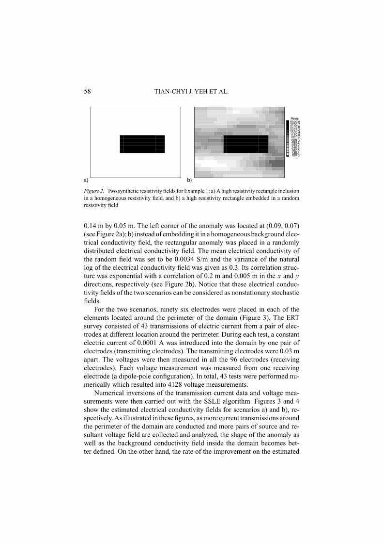
Figure 2. Two synthetic resistivity fields for Example 1: a) A high resistivity rectangle inclusion

in a homogeneous resistivity field, and b) a high resistivity rectangle embedded in a random

resistivity field

0.14 m by 0.05 m. The left corner of the anomaly was located at (0.09, 0.07)(see Figure 2a); b) instead of embedding it in a homogeneous background elec-trical conductivity field, the rectangular anomaly was placed in a randomlydistributed electrical conductivity field. The mean electrical conductivity ofthe random field was set to be 0.0034 S/m and the variance of the naturallog of the electrical conductivity field was given as 0.3. Its correlation struc-ture was exponential with a correlation of 0.2 m and 0.005 m in the x and ydirections, respectively (see Figure 2b). Notice that these electrical conduc-tivity fields of the two scenarios can be considered as nonstationary stochasticfields.

For the two scenarios, ninety six electrodes were placed in each of theelements located around the perimeter of the domain (Figure 3). The ERTsurvey consisted of 43 transmissions of electric current from a pair of elec-trodes at different location around the perimeter. During each test, a constantelectric current of 0.0001 A was introduced into the domain by one pair ofelectrodes (transmitting electrodes). The transmitting electrodes were 0.03 mapart. The voltages were then measured in all the 96 electrodes (receivingelectrodes). Each voltage measurement was measured from one receivingelectrode (a dipole-pole configuration). In total, 43 tests were performed nu-merically which resulted into 4128 voltage measurements.

Numerical inversions of the transmission current data and voltage mea-surements were then carried out with the SSLE algorithm. Figures 3 and 4show the estimated electrical conductivity fields for scenarios a) and b), re-spectively. As illustrated in these figures, as more current transmissions aroundthe perimeter of the domain are conducted and more pairs of source and re-sultant voltage field are collected and analyzed, the shape of the anomaly aswell as the background conductivity field inside the domain becomes bet-ter defined. On the other hand, the rate of the improvement on the estimated

SUCCESSIVE LINEAR ESTIMATOR 59

b)

c)

After a) 5, b) 10, c) 15, d) 20, e) 30, and f) 43 surveys.

1200

1111

1022

933

844

756

667

578

489

400

Low

High

a)

e)

d)

f)

Figure 3. Progression of the estimated resistivity field for case a in example 1 after various

numbers of surveys. The battery symbols indicate the location of the source pair

electrical conductivity field diminishes as the number of current transmissionsincreases.

This example illustrates the intuitive nature of the ERT concept. In essence,ERT is analogous to the human approach inspecting an object: we examinethe object from different angles and perspectives – around the perimeter of theobject. Light is the source, our eyes are the sensors, and our brain providesthe inversion algorithm. Unlike the human brain which provides a “determin-istic” rendering of the object, SSLE interprets signals to yield a statisticallyunbiased image of the object and an uncertainty estimate. This simple exam-ple also demonstrates that an inverse problem can be made better posed ifsufficient and necessary data are collected. Finally, it should be pointed out

60 TIAN-CHYI J. YEH ET AL.

After a) 5, b) 10, c) 15, d) 20, e) 30, f) 43 surveys.

c)

d)

e)

f)

b)

Low

High

a)

50003701

2739

2027

15001111

822

608

450333

247

183

135100

Figure 4. Progression of the estimated resistivity field for case b in example 1 after various

numbers of surveys. The battery symbols indicate the location of the source pair

that a tomographic survey is a technique that allows collection of the necessarydata set, without invasive probing into the domain.

A similar type of survey called electrical impedance tomography (EIT)has been used as a medical imaging device to “seeing” into human bodies(e.g. Mueller et al., 2002). While the concepts of ERT and EIT are similar, thescales of problems and resolution required in these sciences are significantlydifferent. ERT in subsurface is limited by the number of electric potentialsensors and our ability to deploy the sensors to completely surround a geologicmedium to be investigated. The variability of electrical resistivity field ingeologic media is also more complex and larger in magnitude. Therefore, itis expected that uncertainty in ERT is much greater than that in EIT used inmedical sciences.

SUCCESSIVE LINEAR ESTIMATOR 61

3.4.2. EXAMPLE 2

Example 2 illustrates the utility of ERT for characterizing migration of con-taminants in large-scale geological media. Generally speaking, characteriza-tion of transport processes at a field scale based on few local measurementsof contaminant concentrations is highly uncertain. Recent field and numeri-cal experiments (e.g. Kemna et al., 2002; Vanderborght et al., 2005) studyingtransport processes have shown promising results for reducing this uncertaintyusing ERT. The following synthetic 2D study demonstrates the potential of ajoint inversion approach using local concentrations and electrical resistivitymeasurements for reducing uncertainty and enhancing our ability to charac-terize and monitor contaminant movements without extensive invasive andcostly drilling operations.

In this example, migration of a highly electrically conductive solute plumewas simulated in a 2D highly stratified, heterogeneous aquifer with a randomlydistributed hydraulic conductivity field. The aquifer was assumed to be freeof the solute initially and the aquifer had a uniform electrical conductivityfield. A snapshot of the solute plume was then acquired. The concentrationdistribution of the plume was subsequently converted to a bulk electricalconductivity, σ , distribution based on a linear relation:

σ = 0.01 S/m + c · 0.18 S/m (14)

where c is the concentration. This conversion led to an electrical conductivityfield with a maximum at 0.1 S/m and a background of 0.01 S/m (Figure 5a).

This electrical conductivity field was used to simulate the ERT surveyusing electrodes located within three boreholes (see Figures 5b or 5c). Therewere 10 electrodes for each borehole. During the ERT survey a “skip one”dipole-dipole source and measurement array was employed. For each trans-mission, a current of +1 Am or −1 Am is assigned to each electrode of thesource pair. The voltage measurements during each current transmission froma source pair were taken at locations starting from one dipole length (1 m)away from the source along the borehole. In the neighboring borehole, thedipole measurements were started from the bottom electrodes, resulting ineight measurements for each borehole. The survey started with the currenttransmission along the borehole near y = 5 m and voltage measurementsalong the boreholes near y = 5 m and 15 m. The source was then movedto the borehole near y = 15 m and measurements were taken from the threeboreholes. Lastly, the source was moved to the borehole near y = 25 m andmeasurements were taken along the boreholes near y = 15 m and 25 m. Al-together this survey consisted of 8 current transmissions at each boreholeand 316 dipole-dipole measurements. During the simulation as well as theinversion, no flux boundaries were assumed at the right, left and top of the

62 TIAN-CHYI J. YEH ET AL.

0 5 10 15 20 25 30

1

3

5 0.10

0.09

0.07

0.06

0.05

0.04

0.02

0.01

a)

0 5 10 15 20 25 30

1

3

5 0.10

0.09

0.07

0.06

0.05

0.04

0.02

0.01

b)

y [m]

y [m]

y [m]

Z [m

]Z

[m

]Z

[m

]

0 5 10 15 20 25 30

1

3

5 0.10

0.09

0.07

0.06

0.05

0.04

0.02

0.01

c)

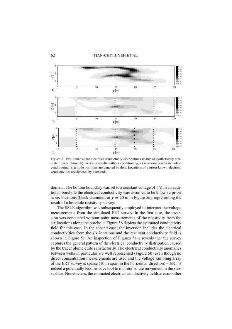
Figure 5. Two dimensional electrical conductivity distributions (S/m): a) synthetically sim-

ulated tracer plume, b) inversion results without conditioning, c) inversion results including

conditioning. Electrode positions are denoted by dots. Locations of a priori known electrical

conductivities are denoted by diamonds

domain. The bottom boundary was set to a constant voltage of 1 V. In an addi-tional borehole the electrical conductivity was assumed to be known a prioriat six locations (black diamonds at y = 20 m in Figure 5c), representing theresult of a borehole resistivity survey.

The SSLE algorithm was subsequently employed to interpret the voltagemeasurements from the simulated ERT survey. In the first case, the inver-sion was conducted without point measurements of the resistivity from thesix locations along the borehole. Figure 5b depicts the estimated conductivityfield for this case. In the second case, the inversion includes the electricalconductivities from the six locations and the resultant conductivity field isshown in Figure 5c. An inspection of Figures 5a–c reveals that the surveycaptures the general pattern of the electrical conductivity distribution causedby the tracer plume quite satisfactorily. The electrical conductivity anomaliesbetween wells in particular are well represented (Figure 5b) even though nodirect concentration measurements are used and the voltage sampling arrayof the ERT survey is sparse (10 m apart in the horizontal direction) – ERT isindeed a potentially less invasive tool to monitor solute movement in the sub-surface. Nonetheless, the estimated electrical conductivity fields are smoother

SUCCESSIVE LINEAR ESTIMATOR 63

than those of the true field in Figure 5a. This is attributed to the fact that SSLEseeks a conditional effective parameter field (see Equation 4), which is smoothif insufficient number of conditioning data sets are included. In other words,had more source/voltage measurements been conducted, the estimated fieldwould have been closer to the true field. This finding also supports results offield experiments by Singha and Gorelick (2005).

Figure 5c shows effects of incorporation of the six point electrical con-ductivity samples from the borehole survey. A comparison of this figure withthe other two clearly indicates that inclusion of the point measurements (con-ditioning using the primary variable) enhances the quality of the inversionresults in terms of the pattern and resistivity values significantly. As a re-sult, the example advocates the integration of ERT surveys with direct pointmeasurements.

3.4.3. EXAMPLE 3

The utility of ERT and the SSLE algorithm is demonstrated for monitoringtransient water infiltration through 3-D vadose zones in this example. Here,water movement was simulated in a 3-D synthetic vadose zone correspondingto an infiltration event. The vadose zone was assumed to be a cube (2 m on eachside) consisting of 2,000 elements in size of 0.2 m × 0.2 m × 0.1 m. Randomvalues of the heterogeneous unsaturated hydraulic parameters were generatedand assigned to each element using the spectral method (see Liu and Yeh,2004). The simulated moisture content distribution at 50,000 minutes afterthe infiltration commenced, θ50,000, (Figure 6a) was used as the true moisturecontent fields for this demonstration. A power law constitutive relation thenrelated the moisture content to the resistivity (e.g. Yeh et al., 2002):

ρ = ρ0θ−m (15)

where ρ is bulk electrical resistivity, ρ0 is a fitting parameter that is related tothe electrical resistivity of pore water, m is a dimensionless fitting parameter,and θ denotes volumetric moisture content. We assumed that ρ0 did notchange during the infiltration event.

This constitutive relation (Equation 15) or a similar type of relation hasfrequently been used by practitioners to translate a resistivity field to a mois-ture content field as well. In addition, a single constitutive relation is oftenassumed for a given entire field. Yeh et al. (2002), however, found that theparameters of Equation (15), ρ0 and m, varied significantly in space underfield conditions. They showed that without considering the spatial variabilityof these parameters, interpretation of moisture content distribution based onEquation (15) can be misleading. In this example, to describe spatial variabilityin the parameters of the resistivity and moisture content relation in the vadose

64 TIAN-CHYI J. YEH ET AL.

x

50100

150y

50100

150

z

0

50

100

150

200

0.280.260.250.230.210.200.18

True θ at t = 50,000 minutes

a)

x

50100

150y

50100

150

z

0

50

100

150

200

Estimated θ at t = 50,000 minutes111 voltages .

b)

x

50100

150y

50100

150

z

0

50

100

150

200

Estimated θ at t = 50,000 minutes111 voltages + 20θ's .

c)

True θ

estim

ated

θ

0.15 0.2 0.25 0.30.15

0.2

0.25

0.3

L1 = 0.0285L2 = 0.00134

e)True θ

estim

ated

θ

0.15 0.2 0.25 0.30.15

0.2

0.25

0.3

L1 = 0.024L2 = 0.0009

f)

x

50100

150y

50100

150

z

0

50

100

150

200

Current source locationsV Location

θ Location

d)

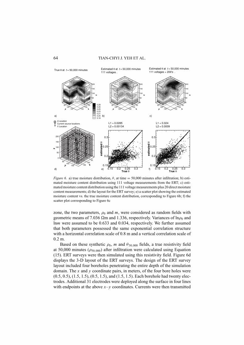
Figure 6. a) true moisture distribution, θ , at time = 50,000 minutes after infiltration; b) esti-

mated moisture content distribution using 111 voltage measurements from the ERT; c) esti-

mated moisture content distribution using the 111 voltage measurements plus 20 direct moisture

content measurements; d) the layout for the ERT survey; e) a scatter plot showing the estimated

moisture content vs. the true moisture content distribution, corresponding to Figure 6b; f) the

scatter plot corresponding to Figure 6c

zone, the two parameters, ρ0 and m, were considered as random fields withgeometric means of 7.036 �m and 1.336, respectively. Variances of lnρ0 andlnm were assumed to be 0.633 and 0.034, respectively. We further assumedthat both parameters possessed the same exponential correlation structurewith a horizontal correlation scale of 0.8 m and a vertical correlation scale of0.2 m.

Based on these synthetic ρ0, m and θ50,000 fields, a true resistivity fieldat 50,000 minutes (ρ50,000) after infiltration were calculated using Equation(15). ERT surveys were then simulated using this resistivity field. Figure 6ddisplays the 3-D layout of the ERT surveys. The design of the ERT surveylayout included four boreholes penetrating the entire depth of the simulationdomain. The x and y coordinate pairs, in meters, of the four bore holes were(0.5, 0.5), (1.5, 1.5), (0.5, 1.5), and (1.5, 1.5). Each borehole had twenty elec-trodes. Additional 31 electrodes were deployed along the surface in four lineswith endpoints at the above x–y coordinates. Currents were then transmitted

SUCCESSIVE LINEAR ESTIMATOR 65

sequentially at the five depths of 0.25, 0.55, 0.95, 1.35, and 1.75 m alongthe upper right bore hole (1.5, 1.5). The ERT surveys resulted in five cur-rent/voltage data sets of 111 voltage measurements each. In addition, we alsosampled 20 ρ0 and m values along each of the four bore holes (a total of 80measurements). The moisture content θ was sampled at 20 locations indicatedby squares in Figure 6d.

To estimate the θ field directly based on the data from the ERT survey,the SSLE algorithm was modified by Liu and Yeh (2004) to include Equa-tion (15), as well as the sample values of ρ0, m, and θ’s. This SSLE is calledthe integrative SSLE. For the purpose of demonstrating the effect of the di-rect θ measurements on the estimated moisture content field, we estimatedthe moisture content distribution at 50,000 minutes for two cases; a) withoutusing any θ measurement and b) with 20 θ measurements in addition to thevoltage measurements.

Figures 6a and 6b show the true moisture content distribution at50,000 minutes and the corresponding estimated moisture content distributionusing 111 × 5 voltage measurements, and 80 pairs of ρ0 and m measurements,respectively. The estimated field using the same number of voltage, ρo andm measurements, but including 20 direct θ measurements, is illustrated inFigure 6c. An inspection of the three figures reveals that the integrative SSLEalgorithm reproduces the general pattern of the simulated true moisture con-tent distribution, even though the constitutive relation between resistivity andmoisture content varies spatially. Again, the estimated moistue content fieldsin Figures 6b and 6c are smoother than that in Figure 6a. The inclusion of the20 θ measurements, on the other hand, greatly improves the estimate of the θ

distribution. Figures 6e and 6f are scatter plots that correspond to Figures 6band 6c, respectively. A 45◦ line indicates perfect estimation (unbiasedness andzero variance); scattering (variance) around the line is indicative of smooth-ness of the estimates. According to these two scatter plots, the inclusion of the20 θ measurements reduces the biasedness of the ERT inversion for moisturecontent. The goodness of fit was also evaluated using L1 and L2 norms. Thereductions in the L1 and L2 norms from Figures 6e to 6f indicate that theaddition of moisture content measurements dramatically improve the estimate.

The conditional variance of the estimate from our SSLE approach can beused to assess the uncertainty associated with the estimate: a smaller con-ditional variance indicates less uncertainty in the estimate. The conditionalvariances corresponding to the estimates obtained when using zero and 20 θ

measurements are shown on Figures 7a and 7b, respectively. Small conditionalvariances are located closely to the four boreholes where secondary informa-tion is measured. At locations where moisture content measurements werecollected, the conditional variance is zero, indicating that these observationsare honored in the inverse model and that no uncertainty exists.

66 TIAN-CHYI J. YEH ET AL.

x (cm)50

100150

y (cm)

50100

150

z (c

m)

0

50

100

150

200

0.0200.0170.0140.0110.0080.0050.002a)

x (cm)50

100150

y (cm)

50100

150

z(c

m)

0

50

100

150

200

0.0200.0170.0140.0110.0080.0050.002b)

Figure 7. Estimation variance maps corresponding to the estimates in Figures 6b and 6c

3.5. Field Study

Previous numerical examples illustrate the ERT concept and robustness ofSSLE. These examples however exclude measurement error and noise. Mea-surement error and noise are associated to equipment resolution and externalelectromagnetic sources (natural or induced) and they are inherent in the real-world applications of ERT. In this section we show an application of ERT tomonitoring leaching operation in a mine site and demonstrate ways to tacklemeasurement error and noise, using our stochastic approach.

As a part of the operation of a test module in the Quebrada Blanca (QB)leaching operation in Northern Chile (see Guzman et al., 2006 for a com-plete description of the experimental setting), an ERT monitoring system wasinstalled early January, 2004. Leaching consists of applying a dilute acid so-lution on the surface of the heap using a drip irrigation system to promote theremoval of metal values. The application rate ranged from 4.2 × 10−4 cm/sto 8.4 × 10−4 cm/s. The duration of the leach cycle is defined as the time atwhich the desire level of metal extraction (e.g. 80%) is attained. The moni-toring system was used to track operational variables (i.e., moisture content,temperature, and oxidation/reduction potential; ORP) for evaluation of theleaching mechanisms within the test module. The system operated during thefirst half of the leach cycle to 12 June 2004 when the system was dismantled.The monitoring system consisted of 34 probes, emplaced at the site with ahorizontal spacing of 1.5 m. Twenty-four probes were installed along the cen-terline of the eastern cell of the test module with dimensions of 80 m by 40 mby 8 m depth; six along a line perpendicular to the centerline on the centerof the cell; and two probes on each of the NW and SE quadrants of the cell.

SUCCESSIVE LINEAR ESTIMATOR 67

Figure 8. Spatial distribution of ERT electrodes at the QB leaching test module

Each probe was equipped with 8 multi-purpose sensors at a vertical intervalof 0.9 m. Figure 8 presents a perspective view of the layout of the monitoringsystem.

To preprocess the voltage data collected from the ERT survey, a sys-tematic approach similar to the structured groundwater model calibrationapproach proposed by Yeh and Mock (1996) was used. Specifically, the for-ward model (Equation 4) is first used to simulate the electric potential fieldin a homogeneous resistivity field at the site, corresponding to an electriccurrent transmission (one pair of source electrodes). The initial value forthe homogeneous electrical resistivity field was obtained based on the rocktype of the site. The simulated electric potential field was then consideredas the mean electric potential field, μ(x). This mean field was comparedwith the measured potential field, constructed by interpolation and extrap-olation using the measured electric potential values. This comparison allowedus to diagnose possible systematic errors in the measurements and/or ourincorrect estimated mean resistivity field. A scatter plot (Figure 9) of the

68 TIAN-CHYI J. YEH ET AL.

Simulated voltages (homogeneous resistivity field)

Fie

ldm

easu

red

volta

ges

-2 -1.5 -1 -0.5 0 0.5 1 1.5 2-2

-1.5

-1

-0.5

0

0.5

1

1.5

2

Upper bound

Lower bound

Figure 9. The scatter plot illustrating how the theoretical voltage variance is used to remove

noisy measurements

measured values versus the observed ones at all of the measurement loca-tions was also utilized for this purpose. After this diagnostic procedure, mea-surements of transmissions with systematic errors were eliminated from thefollowing inversion steps. The variance of the electric potential (σ 2) at eachmeasurement location was determined using Equation (11) afterward. Therequired covariance of the electrical resistivity field in Equation (11) againwas specified using prior information. In this example, the prior informa-tion was merely an initial guess although the covariance could have beenestimated had some borehole resistivity measurements been taken. Noticethat the mean and variance calculation process is embedded in the SSLEalgorithm.

Next, the estimated standard deviation of the potential value at each mea-surement location was used to define a low and an upper bound of the electricpotential measurements (i.e., μ − kσ and μ + kσ , respectively, in which k isan arbitrary integer). Measurements within the upper and the low bound wereconsidered to be statistically reliable given prior knowledge of the spatial vari-ability of the resistivity field at the site. These measurements were selectedfor the inversion process. Figure 9 illustrates this procedure for a selectedtransmission of the electric current.

The simulation domain used for the inversion was 34 m in West-Eastdirection, 57 m in North-south direction, and 9.9 m in vertical direction. Thedomain was discretized into 7106 elements. The corresponding number of

SUCCESSIVE LINEAR ESTIMATOR 69

Figure 10a. Estimated resistivity field at the QB site on 18 Jan. 2004

nodes is 8424. The size of each element was 1.5 m (N-S) by 2.0 m (W-E)by 0.9 m (V). The top and bottom surfaces were assumed to be no-flow andthe other four sides were considered to be constant voltage boundaries with avalue of zero volts. Using the above discretization and boundary conditions,the preprocessed ERT data collected from three different times were analyzed.Figure 10a shows the estimated resistivity field at the site on 18 Jan. 2004. Theestimated field for 24 Feb. 2004 is given in Figure 10b and for 22 March, 2004is in Figure 10c. The total number of measurements used for each inversionwas 2700. The computational time for each case was about 4 hours on a clusterconsisting of four PCs.

While there were no immediate measurements of in-situ moisture con-tent available to validate our estimated resistivity fields, Figures 10a–c showsincreases in volume of low resistivity zones (a general indicator of high mois-ture content) as the irrigation progressed with time. Measurements of mois-ture content during the dismantling of the monitoring system showed goodcorrespondence with estimates of moisture content based on the resistivitymeasurements and lab calibration (Guzman et al., 2006). The evolution ofthe estimated resistivity fields illustrates the progression of the infiltrationprocess. Moreover, the resistivity measurements delineated the strong corre-spondence between moisture distribution and surface topography (i.e., zoneof high resistivity near the surface correspond to topographic highs while

70 TIAN-CHYI J. YEH ET AL.

Figure 10b. Estimated resistivity field at the QB site on 24 Feb. 2004

low resistivity areas, wetter zones, correspond to topographic lows). This isquite encouraging since the topographic relief across the surface of the testmodule is of the order of ±0.5 m. Other factors and procedures as discussedin Example 3 could have possibly improved the accuracy of our estimates.

Figure 10c. Estimated resistivity field at the QB site on 22 March 2004

SUCCESSIVE LINEAR ESTIMATOR 71

Nevertheless, this field case demonstrates the applicability of our SSLE pro-cedure to a real-world ERT data set.

3.6. Discussions and Conclusion

ERT, instead of the traditional resistivity survey, is an inexpensive and viabletechnique for the investigation of subsurface resistivity anomalies. It has beenlisted as one of the most promising near-term science technology targets by aNational Technical Working Group of DOE (NTWG, 2004).

Once a resolution of subsurface electrical resistivity anomalies is definedand necessary and sufficient conditions (Yeh and Simunek, 2002) are given,a 3-D ERT inversion problem can be well posed at least mathematically.While for most field problems, the necessary and sufficient conditions maybe difficult and costly to acquire. A tomographic survey nonetheless offersan intelligent way – common sense – to collect information to make theproblem better posed and the estimate as such increases its resolution. For ill-or better-posed problems, a stochastic estimator (such as SSLE) that seeksthe condition mean estimate and yields an estimate of its uncertainty is anappropriate choice. Note that stationarity and normality are not required forSSLE to derive good estimates but accurate and dense data sets are. However,the implicit stationarity and normality assumptions do affect the uncertaintyderived from SSLE. The uncertainty estimate from any stochastic models,nevertheless, is uncertain itself – statistics is never wrong but can be imprecise.More importantly, the goal of a stochastic estimator is not to predict absoluteuncertainty but to provide a quantitative means to assess effectiveness ofdifferent sampling strategies.

ERT combined with SSLE or an appropriate stochastic estimator is usefulfor environmental applications. However, cautions must be taken if an es-timated resistivity field is translated to other environmental attributes (suchas moisture content, solute concentration, or hydraulic properties of the sub-surface). The ambiguity and the spatial variability of the relation betweengeophysical and other environmental attributes must be considered. For thispurpose, an integrative approach (e.g. Liu and Yeh, 2004) or a stochastic infor-mation fusion approach (e.g. Yeh and Simunek, 2002) is deemed necessary.Likewise, fusion of an ERT survey with a high frequency radar (e.g. groundpenetrating radar) survey may enhance our ability to detect subsurface en-vironmental anomalies at higher resolutions and greater depths than eithersurvey by itself.

Lastly, expanding the concept of ERT to basin- or continental-scale elec-trical resistivity tomographic surveys appears to be logical and feasible al-though it requires high energy sources. Magnetotellurics (e.g. Vozoff, 1991;

72 TIAN-CHYI J. YEH ET AL.

White et al., 2001) in effect is a low frequency, electromagnetic method forcontinental-scale surveys, which has been used for imaging the electrical con-ductivity of the Earth. But it does not have the element of the tomographicsurvey (i.e., examination of the Earth at different angles and perspectives)and its image as such is often equivocal and non-unique. Exploiting cloud-to-ground, direct lightning strikes as a possible energy source (i.e., lightningtomography) for the basin- or continental-scale electromagnetic tomographicsurveys as proposed by Yeh (2005) appears to be a logical future researchtopic in hydrogeophysics.

References

Baker, K., 2001. Investigation of direct and indirect hydraulic property laboratory characteri-

zation methods for heterogeneous alluvial deposits: Application to the Sandia-Tech Vadose

Zone infiltration test site, Masters Thesis, New Mexico Institute of Mining and Technology,

Socorro, NM.

Daily, W., A. Ramirez, D. LaBrecque, and J. Nitao, 1992. Electrical resistivity tomography of

vadose water movement, Water Resour. Res., 28 (5), 1429–1442.

Dettinger, M.D., and J.L. Wilson, 1981. First-order analysis of uncertainty in numerical models

of groundwater flow, 1, Mathematical development, Water Resour. Res., 17, 149–161.

Ellis, R.G., and S.W. Oldenburg, 1994. The pole-pole 3-D dc resistivity inverse problem: A

conjugate gradient approach, Geophys. J. Int., 119, 187–194.

Gavalas, G.R., P.C. Shan, and J.H. Seinfeld, 1976. Reservoir history matching by Bayesian

estimation, Soc. Pet. Eng. J., 337–350.

Gelhar, L.W., 1993. Stochastic Subsurface Hydrology, Prentice Hall, Englewood Cliffs, New

Jersey.

Gutjahr, A., B. Bullard, S. Hatch, and D.L. Hughson, 1994. Joint conditional simulations

and the spectral approach to flow modeling. Stochastic Hydrol. Hydraul., 8 (1), 79–

108.

Guzman, A., R.E. Scheffel, and S.M. Flaherty, 2006. Geochemical Profiling of a Sulfide Leach-

ing OperationA Case Study, SME Annual Convention, March 28–31, 2006, St. Louis, MO,

USA.

Hanna, S., and T.-C.J. Yeh, 1998. Estimation of co-conditional moments of transmissivity,

hydraulic head, and velocity fields, Adv. Water Resour., 22 (1), 87–93.

Hoeksema, R.J., and P.K. Kitanidis, 1984. An application of the geostatistical approach to the

inverse problem in two-dimensional groundwater modeling, Water Resour. Res., 20 (7),

1003–1020.

Hughson, D.L., and T.-C.J. Yeh, 2000. An inverse model for three-dimensional flow in variably

saturated porous media, Water Resour. Res., 36 (4), 829–839.

Kemna, A., J. Vanderborght, B. Kulessa, and H. Vereecken, 2002. Imaging and characterization

of subsurface solute transport using electrical resistivity tomography (ERT) and equivalent

transport models, J. Hydrol., 267, 125–146.

Kitanidis, P.K., 1995. Quasi-linear geostatistical theory for inversing, Water Resour. Res., 31

(10), 2411–2519.

Kitanidis, P.K., 1997. Comment on “A reassessment of the groundwater inverse problem” by

D. McLaughlin and L.R. Townley, Water Resour. Res., 33(9), 2199–2202.

SUCCESSIVE LINEAR ESTIMATOR 73

Kitanidis, P.K., and E.G. Vomvoris, 1983. A geostatistical approach to the inverse problem

in groundwater modeling and one-dimensional simulations, Water Resour. Res., 19 (3),

677–690.

Li, B., and T.-C.J. Yeh, 1998. Sensitivity and moment analysis of head in variably saturated

regimes, Adv. Water Resour., 21 (6), 477–485.

Li, Y., and D.W. Oldenburg, 1994. Inversion of 3D dc-resistivity data using an approximate

inverse mapping, Geophys. J. Int., 116, 527–537.

Li, Y., and D.W. Oldenburg, 2000. Incorporating geological dip information into geophysical

inversions, Geophysics, 65 (1), 148–157.

Liu, S., and T.-C.J. Yeh, 2004. An integrative approach for monitoring water movement in the

vadose zone, Vadose Zone J., 3, 681–692.

Liu, S., T.-C.J. Yeh, and R. Gardiner, 2002. Effectiveness of hydraulic tomography: Sandbox

experiments, Water Resour. Res., 38(4), doi: 10.1029/2001WR000338.

McLaughlin, D., and L. R. Townley, 1996. A reassessment of the groundwater inverse problem,

Water Resour. Res., 32 (5), 1131–1161.

Mueller, J.L., S. Siltanen, and D. Isaacson. A direct reconstruction algorithm for electrical

impedance tomography. IEEE Trans. Med. Imaging, 21 (6), 555–559.

National Research Council (NRC), 2000. Seeing into the earth: noninvasive characterization of

the shallow subsurface for environmental and engineering application, Board on Earth Sci-

ences and Resources, Water Science and Technology Board, Commission on Geosciencce,

Environment, and Resources, National Academy Press, Washington, DC.

National Technical Working Group (NTWG), 2004. Natural and passive remediation of chlo-

rinate solvents: Critical evaluation of science and technology targets, WSRC-TR-2003-

00328, Westinghouse Savannah River Company, Savannah River Site, Aiken, SC 29808,

February 19, 2004.

Oldenburg, D.W., and Y. Li, 1999. Estimating depth of investigation in dc resistivity and Ip

surveys, Geophysics, 64 (2), 403–416.

Sharma, Perm V., 1997. Environmental and Engineering Geophysics, Cambridge University

Press, Cambridge.

Singha, K., and S. Gorelick, 2005. Saline tracer visualized with three-dimensional electri-

cal resistivity tomography: Field-scale spatial moment analysis. Water Resour. Res., 41,

W05023, doi: 10.1029/2004WR003460.

Sun, N.Z., 1994. Inverse Problems in Groundwater Modeling, Kluwer Academic Press,

Norwell, MA.

Sun, N.-Z., and W.W.-G. Yeh, 1992. A stochastic inverse solution for transient groundwater

flow: Parameter identification and reliability analysis, Water Resour. Res., 28 (12), 3269–

3280.

Sykes, J.F., J.L. Wilson, and R.W. Anderews, 1985. Sensitivity analysis for steady state ground-

water flow using adjoint operators, Water Resour. Res., 21 (3), 359–371.

Theis, C.V., 1935. The relation between lowering the piezometric surface and the rate and

duration of discharge of a well using ground water storage, in 16th Annual Meeting of the

Transactions of the American Geophysical Union, Part 2, 519–524.

Tikhonov, A.N., and V.A. Arsenin, 1977. Solutions of Ill-posed Problems. Winston,

Washington.

Vanderborght, J., A. Kemna, H. Hardelauf, and H. Vereecken, 2005. Potential of electrical resis-

tivity tomography to infer aquifer transport characteristics from tracer studies: A synthetic

case study, Water Resour. Res., 41, W06013, doi: 10.1029/2004WR003774.

Vargas-Guzman, J.A., and T.-C.J. Yeh, 1999. Sequential kriging and cokrging: Two powerful

geostatistical approaches, Stochastic Environ. Res. Risk Assess., 13, 416–435.

74 TIAN-CHYI J. YEH ET AL.

Vargas-Guzman, J.A., and T.-C.J. Yeh, 2002. The successive linear estimator: A revisit, Adv.

Water Resour., 25, 773–781.

Vozoff, K., 1991. The magnetotelluric method, in Electromagnetic Methods in Applied Geo-

physics – Applications, Chapter 8, edited by M.N. Nabighia, Society of Exploration Geo-

physicists.

White, B.S., W.E. Kohler, and L.J. Srnka, 2001. Random scattering in magnetotellurics, Geo-

physics, 1, 188–204.

Wu, C.-M., T.-C.J. Yeh, J. Zhu, T.H. Lee, N.-S. Hsu, C.-H. Chen, and A.F. Sancho, 2005.

Traditional analysis of aquifer tests: Comparing apples to oranges?, Water Resour. Res.,

41, W09402, doi: 10.1029/2004WR003717.

Yeh, T.-C.J., 1992. Stochastic modeling of groundwater flow and solute transport in aquifers,

J. Hydrol. Process., 6, 369–395.

Yeh, T.-C.J., 1998. Scale issues of heterogeneity in vadose-zone hydrology, in Scale Dependence

and Scale Invariance in Hydrology, edited by G. Sposito, Cambridge Press, Cambridge,

MA.

Yeh, T.-C.J., 2005. Exploiting natural recurrent stimuli for “seeing” into groundwater basins,

in Fall AGU Meeting, SF.

Yeh, T.-C. J., A.L. Gutjahr, and M. Jin, 1995. An iterative cokriging-like technique for ground-

water flow modeling, Groundwater, 33 (1), 33–41.

Yeh, T.-C.J., and J. Simunek, 2002. Stochastic fusion of information for characterizing and

monitoring the vadose zone, Vadose Zone J., 1, 207–221.

Yeh, T.-C.J., M. Jin, and S. Hanna, 1996. An iterative stochastic inverse method: Conditional

effective transmissivity and hydraulic head fields, Water Resour. Res., 32 (1), 85–92.

Yeh, T.-C.J., and S.Y. Liu, 2000. Hydraulic tomography: Development of a new aquifer test

method, Water Resour. Res., 36 (8), 2095–2105.

Yeh, T.-C.J., S. Liu, R. J. Glass, K. Baker, J. R. Brainard, D. Alumbaugh, and D. LaBrecque, 2002.

A geostatistically based inverse model for electrical resistivity surveys and its applications

to vadose zone hydrology, Water Resour. Res., 38 (12), 1278, doi: 10.1029/2001WR001024.

Yeh, T.-C.J., and P.A. Mock, 1996. A structured approach for calibrating steady-state ground

water flow models, Groundwater, 34 (3), 444–450.

Yeh, T.-C.J., and J. Zhang, 1996. A geostatistical inverse method for variably saturated flow in

vadose zone, Water Resour. Res., 32 (9), 2757–2766.

Yeh, W.W.-G., 1986. Review of parameter identification procedures in groundwater hydrology:

The inverse problem, Water Resour. Res., 22 (1), 95–108.

Zhang, J., and T.-C.J. Yeh, 1997. An iterative geostatistical inverse method for steady flow in

the vadose zone, Water Resour. Res., 33 (1), 63–71.

Zhang, J., R.L. Mackie, and T. Madden, 1995. 3-D resistivity forward modeling and inversion

using conjugate gradients, Geophysics, 60, 1313–1325.

Zhu, J., and T.-C.J. Yeh, 2005. Characterization of aquifer heterogeneity using transient hy-

draulic tomography, Water Resour. Res., 41, W07028, doi: 10.1029/2004WR003790.