Research Reports on Mathematical and Computing SciencesSeries B : Operations Research

Department of Mathematical and Computing Sciences

Tokyo Institute of Technology2-12-1 Oh-Okayama, Meguro-ku, Tokyo 152-8552 Japan

Parallel Implementation of Successive Convex Relaxation Methodsfor Quadratic Optimization Problems

Akiko TakedaToshiba Corporation

(akiko.takeda@toshiba.co.jp)

Katsuki FujisawaDept. of Architecture, Kyoto University

(fujisawa@is-mj.archi.kyoto-u.ac.jp)

Yusuke FukayaNS Solutions Corporation

(Yusuke.Fukaya@open.enicom.co.jp)

Masakazu Kojima

Dept. of Mathematical and Computing Sciences, Tokyo Inst. of Tech.(kojima@is.titech.ac.jp)

May 2001, B-370

Revised September 2001

Abstract. As computing resources continue to improve, global solutions for larger size quadratically-constrained optimization problems become more achievable. In this paper, we focus on larger sizeproblems and get accurate bounds for optimal values of such problems with the successive use of

SDP relaxations on a parallel computing system called Ninf (Network based Information Libraryfor high performance computing).

Key words. Nonconvex Quadratic Program, SDP Relaxation, Lift-and-Project LP relaxation,Lift-and-Project Procedure, Parallel Computation, Global Computing.

1 Introduction

Quadratic optimization is known as one of the most important areas of nonlinear programming. Inaddition to its numerous applications in engineering, a quadratic optimization problem (abbrevi-

ated by QOP) covers various important nonconvex mathematical programs such as 0-1 linear andquadratic integer programs, linear complementarity problems, bilevel quadratic programs, linear

and quadratic fractional programs, and so on. The general class of QOPs can be expressed in thefollowing form:

(QOP)

∣∣∣∣∣max cTx

s.t. γℓ + 2qTℓ x + xT Qℓx ≤ 0 (ℓ = 1, . . .m),

(1)

where c ∈ Rn, qℓ ∈ Rn and Qℓ ∈ Rn×n (ℓ = 1, . . . , m). When a given QOP has a quadraticobjective function such as γ0 +2qT

0 x+xTQ0x, we can transform it into QOP (1) by replacing thequadratic objective function with a new variable t and adding γ0 + 2qT

0 x + xT Q0x = t to the set

of constraints. Therefore, (1) is a general form for quadratically constrained quadratic programs.Pardalos and Vavasis [16] showed that even the simplest quadratic program

min{−x21 + cTx : Ax ≤ b, x ≥ 0}

is an NP-hard problem. Additional quadratic constraints complicate the problem significantly.

As one solution approach to QOP (1), Kojima and Tuncel [9] established a theoretical frame-work of two types of successive convex relaxation methods (abbreviated by SCRMs); one is based on

the lift-and-project LP (linear programming) relaxation and the other based on the SDP (semidef-inite programming) relaxation. We can regard SCRMs as extensions of the lift-and-project proce-

dure, which was proposed independently by Lovasz and Schrijver [11] and Sherali and Adams [20]for 0-1 integer programs, to QOP (1).

We denote the feasible region of QOP (1) by F , that is,

F ≡ {x ∈ Rn : γℓ + 2qTℓ x + xTQℓx ≤ 0 (ℓ = 1, . . . , m)}.

Here we suppose that F is bounded and is included in a known compact convex set C0, i.e.,F ⊆ C0. Starting from the initial convex relaxation C0 of F , an SCRM successively constructs

tighter convex relaxations Ck (k = 1, 2, . . .) of F with the successive use of the lift-and-projectLP or SDP relaxation. Therefore, maximizing the linear objective function cTx of QOP (1)

over Ck (k = 0, 1, 2, . . .), we successively obtain better upper bounds {ζk (k = 0, 1, 2, . . .)} forthe maximal objective function value of QOP (1). While the SCRMs proposed by [9] enjoy

the global convergence property that ∩+∞

k=0Ck = the convex hull of F , they involve an infinitenumber of semi-infinite LPs or SDPs to generate a new convex relaxation Ck of F . To resolve thisdifficulty, Kojima and Tuncel [10] proposed implementable versions of SCRMs by bringing two new

techniques, “discretization” and “localization”, into their theoretical framework. Their techniquesallow us to solve finitely many LPs or SDPs having finitely many inequality constraints, so that the

discretized-localized versions are implementable on a computer. However, they are still impracticalbecause as a higher accuracy upper bound is required for the maximal objective function value of

QOP (1), not only the number of LPs or SDPs to be solved but also their sizes explode quite rapidly.More recently, Takeda, Dai, Fukuda and Kojima [24] presented practical SCRMs, which overcame

such a rapid explosion by further slimming down the discretized-localized SCRMs. Although thesepractical methods are no more guaranteed to achieve an upper bound with a prescribed accuracy,

the numerical results reported in the paper [24] are promising.

1

In this paper, we propose parallel versions of practical SCRMs. For constituting Ck (k =1, 2, . . .), SCRMs generate a large number of LPs or SDPs at each iteration. Our parallel imple-

mentation of SCRMs process those multiple LPs or SDPs simultaneously using multiple processors.To enhance the effect of parallel computing, we reduce the work of a client machine, and also de-crease communication between processors as much as possible. We implement a highly parallel

algorithm on a client-server based parallel computing system called Ninf (Network based Informa-tion Library for high performance computing) [18, 19]. Moreover, our parallel implementation of

SCRMs adopt new construction for Ck (k = 1, 2, . . .) so that the number of constraints of eachLP or SDP is considerably decreased. As a result, we can deal with some larger size QOPs, which

existing SCRMs cannot process.

This paper consists of five sections. In Section 2, we introduce basic discretized-localized

SCRMs with the use of the lift-and-project LP and SDP relaxations, and present a serial imple-mentation of SCRMs. In Section 3, we present new variants of discretized-localized SCRMs suit-

able for parallel computing, and show a parallel implementation of the new discretized-localizedSCRMs. In Section 4, we report its numerical results implemented on Ninf. In Section 5, we give

some concluding remarks.

2 Successive Convex Relaxation Methods

We will overview a basic discretized-localized SCRM according to the recent paper [24], which dis-

cussed some implementation details of discretized-localized SCRMs and gave preliminary numericalresults. We introduce a standard serial algorithm of discretized-localized SCRMs in Section 2.1,and we present some basic properties on the algorithm in Section 2.2.

2.1 Preliminaries

The previous works [8, 9, 10, 24, 25] of SCRMs handled general quadratic optimization problems(abbreviated by QOPs) with the following form:

max{cTx : x ∈ F}, (2)

where

F ≡ {x ∈ C0 : qf(x; γ, q, Q) ≤ 0 (∀qf(·; γ, q, Q) ∈ P F )},

C0 ≡ a given compact convex set including F ; we assume that C0 is

represented in terms of linear inequalities when we are concerned

with SCRMs using the lift-and-project LP relaxation, while we assume

that C0 is represented in terms of linear matrix inequalities

when we are concerned with SCRMs using the SDP relaxation,

qf(x; γ, q, Q) ≡ γ + 2qT x + xT Qx (∀x ∈ Rn),

PF ≡ {γℓ + 2qTℓ x + xTQℓx : ℓ = 1, . . . , m}.

To describe a basic discretized-localized SCRM, we introduce the following notation:

Sn : the set of n × n symmetric matrices,

2

Sn+ : the set of n × n positive semidefinite symmetric matrices,

Q •X ≡ the inner product of two symmetric

matrices Q and X, i.e., Q • X ≡∑

i

∑

j

QijXij,

D = {d ∈ Rn : ‖d‖ = 1} (the set of unit vectors in Rn),

D0 ⊂ D : a finite set of unit direction vectors,

ei : the ith unit coordinate vector (i = 1, . . . , n).

For ∀d0 ∈ D0, ∀d ∈ D, ∀x ∈ Rn and ∀ compact convex subset C of Rn, we define

α(C, d) ≡ sup{dT x : x ∈ C},ℓsf (x; C, d) ≡ dTx − α(C, d),

r2sf(x; C, d0, d) ≡ −(dT0 x − α(C0, d0))(d

Tx − α(C, d)).

(3)

We call ℓsf (·; C, d) a linear supporting function for C in a direction d ∈ D, r2sf(·; C, d0, d) a

rank-2 (quadratic) supporting function for C in a pair of directions d0 ∈ D0 and d ∈ D. Let

PL(C, D) ≡ {ℓsf(·; C, d) : d ∈ D}, (∀D ⊆ D),

P2(C, D0, D) ≡ {r2sf(·; C, d0, d) : d0 ∈ D0, d ∈ D} (∀D ⊆ D).

}

(4)

Now we summarize a basic discretized-localized SCRM (Algorithm 2.1 below) proposed by

[10, 24]. At each iteration (say, the kth iteration) of the basic SCRM, we choose a finite direction-set Dk ⊆ D, compute α(Ck, d) for ∀d ∈ Dk, and construct a function-set P2(Ck, D0, Dk) using

α(C0, d0) (∀d0 ∈ D0) and α(Ck, d) (∀d ∈ Dk). Note that Pk = P2(Ck, D0, Dk) ∪ PL(C0, D0)induces valid inequalities for the kth iterate Ck. That is, any function qf(·; γ, q, Q) of P k satisfies

qf(x; γ, q, Q) ≤ 0 for every x ∈ Ck.

Since Ck was chosen to include F at the previous iteration, each qf(x; γ, q, Q) ≤ 0 serves as a(redundant) valid inequality for F ; hence F is represented as

F = {x ∈ C0 : qf(x; γ, q, Q) ≤ 0 (∀qf(·; γ,q, Q) ∈ P F ∪ Pk)}. (5)

We then apply the lift-and-project LP or SDP relaxation to the region F with the representation

of (5), and obtain the region

FL(C0,PF ∪ Pk) =

{

x ∈ C0 :∃X ∈ Sn such thatγ + 2qTx + Q •X ≤ 0 (∀qf(·; γ, q, Q) ∈ PF ∪ Pk)

}

(6)

= a lift-and-project LP relaxation of F

with the use of the representation PF ∪ Pk

or

F (C0,PF ∪ Pk) =

x ∈ C0 :

∃X ∈ Sn such that

(1 xT

x X

)

∈ S1+n+ ,

γ + 2qTx + Q • X ≤ 0 (∀qf(·; γ, q, Q) ∈ PF ∪ Pk)

, (7)

= an SDP relaxation of F with the use of the representation P F ∪ Pk.

Each region corresponds to the (k + 1)th iterate Ck+1. By definition, it is clear that Ck+1 is aconvex subset of C0 and that F ⊆ Ck+1.

3

Algorithm 2.1. (Serial implementation of a basic discretized-localized SCRM)

Step 0: Let D0 ⊆ D. Compute

α(C0, d0) = max{dT0 x : x ∈ C0} (∀d0 ∈ D0),

and construct PL(C0, D0) according to (3) and (4). Let C1 = C0 and k = 1.

Step 1: Compute an upper bound ζk of the maximum objective function value of QOP (2) by

ζk = max{cT x : x ∈ Ck}. If ζk satisfies some termination criteria, then stop.

Step 2: Choose a finite direction-set Dk ⊆ D. Compute

α(Ck, d) = max{dT x : x ∈ Ck} (∀d ∈ Dk).

Step 3: Construct a set P k = P2(Ck, D0, Dk) ∪ PL(C0, D0) according to (3) and (4).

Step 4: Let Ck+1 = FL(C0,PF ∪ Pk) or Ck+1 = F (C0,PF ∪ Pk).

Step 5: Let k = k + 1, and go to Step 1.

Note that the problem max{dT0 x : x ∈ C0} to be solved in Step 0 is either an LP or an SDP

since we have assumed that C0 is represented in terms of either linear inequalities or linear matrix

inequalities. Also, in Step 2, we solve LPs over the polyhedral feasible region Ck = FL(C0,PF ∪

Pk−1) described in terms of linear inequalities or SDPs over the convex feasible region Ck =

F (C0,PF ∪ Pk−1) described in terms of linear matrix inequalities to obtain α(Ck, d) for ∀d ∈ Dk

(k = 1, 2, . . .). We will give a termination criteria used in our numerical experiments in Section 4.2.

Algorithm 2.1 above lacks a description for the direction-sets Dk (k = 0, 1, 2, . . .). In previous works[9, 10, 24, 25], SCRMs commonly utilized D 0 such as

D0 = {e1, . . . , en,−e1, . . . ,−en}, (8)

and adopted various kinds of direction-sets Dk ⊆ D (k = 1, 2, . . . ).

Algorithm 2.1 with the above choice of D0 and Dk ⊆ D (k = 1, 2, . . . ) generates a sequence of

convex sets Ck ⊆ C0 (k = 1, 2, . . . ) and a sequence of real numbers ζk (k = 1, 2, . . . ) satisfying

C0 ⊇ Ck ⊇ Ck+1 ⊇ F (k = 1, 2, . . . ),

ζk ≥ ζk+1 ≥ ζ∗ ≡ sup{cT x : x ∈ F} (k = 1, 2, . . . ).

If we took Dk = D (k = 1, 2, . . . ), Ck (k = 1, 2, . . . ) would converge to the convex hull of F and ζk

(k = 1, 2, . . . ) to an optimal value ζ ∗ of QOP (2) as k → ∞. However, such SCRMs with Dk = D(k = 1, 2, . . . ) are conceptual and not implementable, because they involve an infinite number of

LPs or SDPs to be solved at each iteration. See [9] for more details of conceptual SCRMs.

To implement Algorithm 2.1 on a computer, it is necessary to choose a finite set of directionsfor Dk at the kth (k = 1, 2, . . .) iteration. In the remainder of the paper, we take

Dk ≡ { bi+(θk), bi−(θk), i = 1, 2, . . . , n} (9)

with a parameter θk ∈ (0, π/2] according to the paper [24]. Here,

bi+(θ) =c cos θ + ei sin θ

νi+(θ), bi−(θ) =

c cos θ − ei sin θ

νi−(θ)

νi+(θ) = ‖c cos θ + ei sin θ‖, νi−(θ) = ‖c cos θ − ei sin θ‖.

4

Then P2(Ck, D0, Dk) consists of 4n2 quadratic functions such that

P2(Ck, D0, Dk) =

r2sf(x; Ck,−ej, bi+(θk)), r2sf(x; Ck, ej, bi−(θk))r2sf(x; Ck, ej , bi+(θk)), r2sf(x; Ck,−ej, bi−(θk))

i = 1, . . . , n, j = 1, . . . , n

. (10)

See (3) and (4). We will call Algorithm 2.1 DLSLP if it takes the finite direction-sets D k (k =

0, 1, 2, . . . ) introduced above and the lift-and-project LP relaxation FL(C0,PF ∪ Pk) in Step 4,

while we call Algorithm 2.1 DLSSDP if it takes the finite direction-sets D k (k = 0, 1, 2, . . . ) aboveand the SDP relaxation F (C0,PF ∪ Pk) for Ck+1 in Step 4.

We choose θ1 = π/2 at the first iteration of Algorithm 2.1. In this case, the vectors b i+(θ1)and bi−(θ1) of D1 turn out to be the ith unit coordinate vector ei and its minus −ei, respectively.

Then, the values α(C1, ei) and −α(C1,−ei) correspond upper and lower bounds for the variablexi, respectively. Hence the set P2(C1, D0, D1) constructed in Step 3 of Algorithm 2.1 containsall rank-2 quadratic functions induced from the pairwise products of lower and upper bounding

constraints for variables xi (i = 1, 2, . . . , n). These constraints correspond to underestimatorsand overestimators of quadratic terms xixj (i, j = 1, 2, . . . , n), which were introduced in [13] and

have been used as lower (or upper) bounding techniques of some branch-and-bound methods (forinstance, see [17, 28]). We also see that both b i+(θ) and bi−(θ) (i = 1, . . . , n) approach to the

objective direction c as θ → 0.

2.2 Some Properties of SCRMs

Two important key words in this section are “linearized” and “convexified.” To explain thesewords, we will utilize Lemma 2.2, Examples 2.3 and 2.4 below.

We write the set Q+ of convex quadratic functions on Rn and the set L of linear functions onRn as

Q+ ≡ {qf(·; γ, q, Q) : γ ∈ R, q ∈ Rn, Q ∈ Sn+},

L ≡ {qf(·; γ, q, Q) : γ ∈ R, q ∈ Rn, Q = O},

respectively. Let c.cone(P) denote the convex cone generated by a set P of quadratic functions;

c.cone(P) ≡

{ℓ∑

i=1

λi pi(·) : λi ≥ 0, pi(·) ∈ P (i = 1, 2, . . . , ℓ), ℓ ≥ 0

}

.

Lemma 2.2. 1 (Theorem 2.4 and Corollary 2.5 of Kojima and Tuncel [9])

(i) FL(C0,PF ∪ Pk) ⊂ {x ∈ C0 : p(x) ≤ 0 (∀p(·) ∈ c.cone(PF ∪ Pk) ∩ L)},

(ii) F (C0,PF ∪ Pk) ⊂ {x ∈ C0 : p(x) ≤ 0 (∀p(·) ∈ c.cone(PF ∪ Pk) ∩Q+)}.

1Kojima and Tuncel [9] presented a stronger result in which the equalities hold in (i) and (ii) below. Their prooffor the ⊃ part is incomplete but the ⊂ remains valid. See also Fujie and Kojima [5]

5

Figure 1: Feasible Region F of Example 2.3

(1,0)

(0,1)

x1

(1,1)

x2

F x1 + x2 = 23/16

Example 2.3. Let

C0 ≡ {(x1, x2) : 0 ≤ x1 ≤ 1, 0 ≤ x2 ≤ 1},

PF ≡ {−x1, x1 − 1, −x2, x2 − 1, −(x1 − 1)2 − (x2 − 1)2 + (3

4)2},

F ≡ {(x1, x2) ∈ C0 : qf(x1, x2; γ, q, Q) ≤ 0 (∀qf(·; γ, q, Q) ∈ P F )

=

{(x1, x2) : 0 ≤ x1 ≤ 1, 0 ≤ x2 ≤ 1, −(x1 − 1)2 − (x2 − 1)2 + (

3

4)2 ≤ 0

}.

The shaded area of Figure 1 illustrates the feasible region F . Take θ1 = π/2 at the first iteration

of Algorithm 2.1. Then Step 3 of Algorithm 2.1 constructs a finite set P 2(C1, D0, D1) of quadraticfunctions including x2

1 − x1 and x22 − x2. The addition of x2

1 − x1 ≤ 0 and x22 − x2 ≤ 0 to the

nonconvex quadratic inequality constraint

−(x1 − 1)2 − (x2 − 1)2 + (3

4)2 ≤ 0 (11)

involved in the description of F removes the nonconvex quadratic terms −x21 and −x2

2 of (11), and

generates a linear inequality

x1 + x2 −23

16≤ 0. (12)

Since

x1 + x2 −23

16∈ c.cone(PF ∪ P1)∩ L,

we see by Lemma 2.2 that any point x of a lift-and-project LP relaxation C2 = FL(C0,PF ∪ P1)

satisfies (12). As we see in Figure 1, the linear inequality (12) cuts off the initial convex relaxationC0 of the feasible region F effectively. We may regard the inequality (12) as a linear relaxation of

the nonconvex quadratic constraint (11) with the help of two quadratic functions x21−x1 and x2

2−x2

in P2(C1, D0, D1). We say that the nonconvex quadratic function −(x1−1)2−(x2−1)2+(34 )2 in PF

is linearized with the help of quadratic functions in P 2(C1, D0, D1). The set c.cone(PF ∪ P1) ∩ Lconsists of all linerlizations of quadratic functions qf(·; γ ℓ, qℓ, Qℓ) ∈ PF with the help of quadratic

functions in P2(C1, D0, D1).

Example 2.4. Let

C0 ≡ {(x1, x2) : 0 ≤ x1 ≤ 1, 0 ≤ x2 ≤ 1},

6

Figure 2: Feasible Region F of Example 2.4

(0,1)

x1

(1,1)

x2

F

x1 - x2 = 1/42

PF ≡ {−x1, x1 − 1, −x2, x2 − 1, x21 − x2

2 −1

4},

F ≡

{(x1, x2) ∈ C0 : x2

1 − x22 −

1

4≤ 0

}

=

{(x1, x2) : 0 ≤ x1 ≤ 1, 0 ≤ x2 ≤ 1, x2

1 − x22 −

1

4≤ 0

}.

As in the previous example, we take θ1 = π/2 and construct a finite set P2(C1, D0, D1) including

the quadratic function x22 − x2 in Step 3 of Algorithm 2.1. Now we can remove the nonconvex

quadratic term −x22 of the function x2

1 − x22 −

14 in PF by adding the quadratic function x2

2 − x2

to generate a convex quadratic function x21 − x2 −

14 in c.cone(PF ∪ P1). Hence we know that

C2 = F (C0,PF ∪ P1) ⊂ {(x1, x2) ∈ C0 : x21 − x2 −

1

4≤ 0}.

Thus the quadratic function x21−x2

2−14 in PF is convexified with the help of the quadratic function

x22−x2 in P2(C1, D0, D1). The set c.cone(PF ∪P1)∩Q+ consists of all convexifications of quadratic

functions qf(·; γℓ, qℓ, Qℓ) ∈ PF with the help of quadratic functions in P 2(C1, D0, D1).

Generally, to linearize (or convexify) each quadratic function qf (·; γ ℓ, qℓ, Qℓ) of PF , the DLSLP

and DLSSDP utilize an “atomic rank-1” quadratic function with only one quadratic term x ixj

in c.cone(P2(Ck, D0, Dk)), which is constructed as a nonnegative combination of two functions

r2sf(·; Ck,−ej , bi+(θ)) and r2sf(·; Ck, ej, bi−(θ)) in P2(Ck, D0, Dk), such that

pij(x) ≡νi+(θ)

2 sinθr2sf(x; Ck,−ej, bi+(θ)) +

νi−(θ)

2 sin θr2sf(x; Ck, ej, bi−(θ))

= xTeieTj x + (aT

ijx + βij).

(13)

Here

aij =1

2 tan θ{α(C0,−ej) + α(C0, ej)} c

+1

2{α(C0,−ej) − α(C0, ej)} ei

+1

2 sin θ{νi−(θ)α(Ck, bi−(θ)) − νi+(θ)α(Ck, bi+(θ))} ej,

βij = −1

2 sin θ{νi+(θ)α(C0,−ej)α(Ck, bi+(θ)) + νi−(θ)α(C0, ej)α(Ck, bi−(θ))} .

(14)

7

A nonnegative combination of some other two functions in P 2(Ck, D0, Dk) leads to another “atomicrank-1” quadratic functions with only one quadratic term −xixj as

p′ij(x) ≡νi+(θ)

2 sinθr2sf(x; Ck, ej , bi+(θ)) +

νi−(θ)

2 sin θr2sf(x; Ck,−ej, bi−(θ))

= −xT eieTj x + (a′

ijTx + β′

ij) (i, j = 1, 2, . . . , n).

(15)

Here a′

ij ∈ Rn and β′

ij ∈ R have similar representations to aij ∈ Rn and βij ∈ R given in (14),respectively. We see by definition that pij(x), p′ij(x) ∈ c.cone(Pk) for i, j = 1, . . . , n. Hencec.cone(PF ∪ Pk) includes the following linear function gℓ(x).

gℓ(x) ≡ qf (x; γℓ, qℓ, Qℓ) +∑

(i,j)

Q(i,j)ℓ+ p′ij(x) −

∑

(i,j)

Q(i,j)ℓ− pij(x)

= (γℓ +∑

(i,j)

Q(i,j)ℓ+ β′

ij −∑

(i,j)

Q(i,j)ℓ− βij) + (2qℓ +

∑

(i,j)

Q(i,j)ℓ+ a′

ij −∑

(i,j)

Q(i,j)ℓ− aij)

Tx,

(16)

where Q(i,j)ℓ denotes the (i, j)th element of the matrix Qℓ and

Q(i,j)ℓ+ =

{Q

(i,j)ℓ if Q

(i,j)ℓ > 0

0 otherwise,Q

(i,j)ℓ− =

{Q

(i,j)ℓ if Q

(i,j)ℓ < 0

0 otherwise.

Thus we obtain gℓ(·) ∈ c.cone(PF ∪Pk)∩L with the help of quadratic functions in P2(C1, D0, D1),and an associated linear valid inequality gℓ(x) ≤ 0 for the feasible region F of QOP (2). In general,

we can expect that c.cone(PF ∪Pk)∩L involves linearizations of the function qf(·; γℓ, qℓ, Qℓ) ∈ PF

which induce more effective valid inequalities than gℓ(x) ≤ 0 constructed above.

Similarly we can derive a convexification of each quadratic function qf(·; γℓ, qℓ, Qℓ) ∈ PF .In this case, we restrict ourselves to a nonconvex part of qf(·; γℓ, qℓ, Qℓ) ∈ PF . Suppose thatQℓ = Q+

ℓ +Q−

ℓ with a positive semidefinite Q+ℓ and a negative semidefinite Q−

ℓ . Then we see that

qf(·; γℓ, qℓ, Qℓ) = qf(·; γℓ, qℓ, Q+ℓ ) + qf(·; 0, 0, Q−

ℓ ).

Now we can apply the same argument as above to construct a linearization g−

ℓ (·) of qf (·; 0, 0, Q−

ℓ )with the help of “atomic rank-1” quadratic functions p ij(·) and p′ij(·) (i, j = 1, 2, . . . , n). Finally

we obtain qf (·; γℓ, qℓ, Q+ℓ ) + g−ℓ (·) ∈ c.cone(PF ∪ Pk)∩ Q+.

3 Parallel Implementation of SCRMs

In Step 2 of Algorithm 2.1, 2n problems (LPs or SDPs) involving 4n2 additional quadratic con-

straints are generated for constructing P 2(Ck, D0, Dk). It should be emphasized that these 2nproblems are independent and they can be processed in parallel. In this section, we consider

parallel computation of those problems. Although parallel computation is much help to reducecomputational time drastically, 4n2 constraints of each problem become an obstacle when we solve

a large size QOP (2). In Section 3.1, we design new SCRMs so that each LP or SDP has a fewernumber of constraints than 4n2. Then, in Section 3.2, we will modify Algorithm 2.1 and present

a parallel algorithm for a client-server based parallel computing system.

8

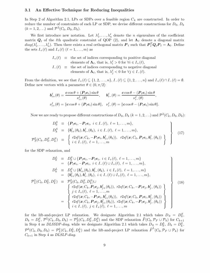
3.1 An Effective Technique for Reducing Inequalities

In Step 2 of Algorithm 2.1, LPs or SDPs over a feasible region Ck are constructed. In order to

reduce the number of constraints of each LP or SDP, we devise different constructions for D0, Dk

(k = 1, 2, . . .) and P 2(Ck, D0, Dk).

We first introduce new notation. Let λℓ1, . . . , λ

ℓn denote the n eigenvalues of the coefficient

matrix Qℓ of the ℓth quadratic constraint of QOP (2), and let Λℓ denote a diagonal matrixdiag(λℓ

1, . . . , λℓn). Then there exists a real orthogonal matrix P ℓ such that P T

ℓ QℓP ℓ = Λℓ. Define

the sets I+(ℓ) and I+(ℓ) (ℓ = 1, . . . , m) as

I+(ℓ) ≡ the set of indices corresponding to positive diagonalelements of Λℓ, that is, λℓ

i > 0 for ∀i ∈ I+(ℓ),

I−(ℓ) ≡ the set of indices corresponding to negative diagonalelements of Λℓ, that is, λℓ

j < 0 for ∀j ∈ I−(ℓ).

From the definition, we see that I+(ℓ) ⊆ {1, 2, . . . , n}, I−(ℓ) ⊆ {1, 2, . . . , n} and I+(ℓ)∩ I−(ℓ) = ∅.Define new vectors with a parameter θ ∈ (0, π/2]:

bℓi+(θ) =

c cos θ + (P ℓei) sinθ

νℓi+(θ)

, bℓi−(θ) =

c cos θ − (P ℓei) sin θ

νℓi−(θ)

,

νℓi+(θ) = ‖c cos θ + (P ℓei) sin θ‖, νℓ

i−(θ) = ‖c cos θ − (P ℓei) sinθ‖.

Now we are ready to propose different constructions of D0, Dk (k = 1, 2, . . .) and P 2(Ck, D0, Dk):

DS0 ≡ {P ℓei,−P ℓei, i ∈ I−(ℓ), ℓ = 1, . . . , m},

DSk ≡ {bℓ

i+(θk), bℓi−(θk), i ∈ I−(ℓ), ℓ = 1, . . . , m},

P2S(Ck, DS

0 , DSk ) ≡

{r2sf(x; Ck,−P ℓei, b

ℓi+(θk)), r2sf(x; Ck, P ℓei, b

ℓi−(θk))

i ∈ I−(ℓ), ℓ = 1, . . . , m

}

(17)

for the SDP relaxation, and

DL0 ≡ DS

0 ∪ {P ℓei,−P ℓei, i ∈ I+(ℓ), ℓ = 1, . . . , m}= {P ℓei,−P ℓei, i ∈ I−(ℓ)∪ I+(ℓ), ℓ = 1, . . . , m},

DLk ≡ DS

k ∪ {bℓi+(θk), bℓ

i−(θk), i ∈ I+(ℓ), ℓ = 1, . . . , m}= {bℓ

i+(θk), bℓi−(θk), i ∈ I−(ℓ) ∪ I+(ℓ), ℓ = 1, . . . , m},

P2L(Ck, D

L0 , DL

k ) ≡ P2S(Ck, DS

0 , DSk )∪{

r2sf(x; Ck, P ℓej, bℓj+(θk)), r2sf(x; Ck,−P ℓej, b

ℓj−(θk))

j ∈ I+(ℓ), ℓ = 1, . . . , m

}

=

r2sf(x; Ck,−P ℓei, bℓi+(θk)), r2sf(x; Ck, P ℓei, b

ℓi−(θk))

r2sf(x; Ck, P ℓej , bℓj+(θk)), r2sf(x; Ck,−P ℓej , b

ℓj−(θk))

i ∈ I−(ℓ), j ∈ I+(ℓ), ℓ = 1, . . . , m

(18)

for the lift-and-project LP relaxation. We designate Algorithm 2.1 which takes D 0 = DS0 ,

Dk = DSk , P2(Ck, D0, Dk) = P2

S(Ck, DS0 , DS

k ) and the SDP relaxation F (C0,PF ∪ Pk) for Ck+1

in Step 4 as DLSSDP-diag, while we designate Algorithm 2.1 which takes D0 = DL0 , Dk = DL

k ,

P2(Ck, D0, Dk) = P2L(Ck, DL

0 , DLk ) and the lift-and-project LP relaxation F

L(C0,PF ∪ Pk) for

Ck+1 in Step 4 as DLSLP-diag.

9

We will show how each quadratic function qf (·; γℓ, qℓ, Qℓ) of PF is convexified in DLSSDP-diagwith the help of quadratic functions of P2

S(Ck, DS0 , DS

k ). First note that each coefficient matrix

Qℓ of the quadratic constraints of QOP (2) can be expressed as Qℓ = Q+ℓ + Q−

ℓ using a positivesemidefinite definite matrix Q+

ℓ and a negative semidefinite definite matrix Q−

ℓ ;

Q+ℓ ≡

∑

i∈I+(ℓ)

λℓi(P ℓei)(P ℓei)

T and Q−

ℓ ≡∑

i∈I−

(ℓ)

λℓi(P ℓei)(P ℓei)

T .

As a nonnegative combination of two functions of P 2S(Ck, DS

0 , DSk ), we have an “atomic rank-1”

quadratic function

pℓi(x) ≡

νℓi+(θk)

2 sin θk

r2sf(x; Ck,−P ℓei, bℓi+(θk)) +

νℓi−(θk)

2 sin θk

r2sf(x; Ck, P ℓei, bℓi−(θk))

= xT (P ℓei)(P ℓei)Tx + (aℓ

i)Tx + βℓ

i (i ∈ I−(ℓ))

for some aℓi ∈ Rn and βℓ

i ∈ R. Then, using these atomic rank-1 quadratic functions pℓi(x)

(i ∈ I−(ℓ)), we can convexify the quadratic function qf(·; γℓ, qℓ, Qℓ) such that

hℓ(x) = (γℓ + 2qTℓ x + xTQℓx) −

∑

i∈I−

(ℓ)

λℓi pℓ

i(x)

= (γℓ −∑

i∈I−

(ℓ)

λℓi βℓ

i ) + (2qℓ −∑

i∈I−

(ℓ)

λℓi aℓ

i)T x + xT Q+

ℓ x.

(19)

Thus we have obtained hℓ(·) ∈ c.cone(PF ∪ Pk) ∩ Q+, which induces a convex quadratic validinequality hℓ(x) ≤ 0 for the feasible region F of QOP (2).

To linearize the quadratic function qf (·; γℓ, qℓ, Qℓ) of PF , we further need quadratic functionsin the difference set P2

L(Ck, DL0 , DL

k )\P2S(Ck, DS

0 , DSk ). As a nonnegative combination of two func-

tions in this difference set, we have

pℓj(x) ≡

νℓj+(θk)

2 sinθk

r2sf(x; Ck, P ℓej, bℓj+(θk)) +

νℓj−(θk)

2 sin θk

r2sf(x; Ck,−P ℓej, bℓj−(θk))

= −xT (P ℓej)(P ℓej)Tx + (aj)

ℓT x + βjℓ (j ∈ I+(ℓ))

for some aℓj ∈ Rn and βℓ

j ∈ R. Now we obtain a linear function in c.cone(PF ∪ P2L(Ck, D

L0 , DL

k ))such that

hℓ(x) ≡ hℓ(x) +∑

j∈I+(ℓ) λℓj pℓ

j(x)

= (γℓ +∑

j∈I+(ℓ)

λℓj βj

ℓ −∑

i∈I−

(ℓ)

λℓi βℓ

i ) + (2qℓ +∑

j∈I+(ℓ)

λℓj aℓ

j −∑

i∈I−

(ℓ)

λℓi aℓ

i)Tx,

(20)

and an associated linear valid inequality hℓ(x) ≤ 0 for the feasible region F of QOP (2).

Table 1 shows the number of SDPs or LPs to be solved at every iteration and the number

of constraints each problem has, comparing four variants of the SCRMs which we have discussedso far. |P | denotes the number of elements contained in the set P . The entries of Table 1 are

computed as

#SDPs = |Dk|, #LPs = |Dk| and #const. = |P2(Ck, D0, Dk)|.

It should be noted that∑m

ℓ=1 |I−(ℓ)| ≤∑m

ℓ=1(|I+(ℓ)| + |I−(ℓ)|) ≤ mn. Hence, if m ≤ 2n holdsbetween the number of constraints m and the number of variables n for QOP (2), “#const.” of

10

Table 1: Comparison among four SCRMs

methods #SDPs #LPs #const.

DLSSDP 2n 4n2

DLSSDP-diag 2∑m

ℓ=1 |I−(ℓ)| 2∑m

ℓ=1 |I−(ℓ)|DLSLP 2n 4n2

DLSLP-diag 2∑m

ℓ=1(|I+(ℓ)|+ |I−(ℓ)|) 2∑m

ℓ=1(|I+(ℓ)|+ |I−(ℓ)|)

Figure 3: The client-server based parallel computing system

ClientProgram

ClientMachine

Server Machine 1

........

Server Machine V

Numerical Library

Network

DLSSDP-diag (or DLSLP-diag) is smaller than that of DLSSDP (or DLSLP). In the test problems

of QOP (2) of our numerical experiments reported in Section 4, the number of SDPs (or LPs) tobe solved in DLSSDP-diag (or DLSLP-diag) is larger than that in DLSSDP (or DLSLP), whileeach problem generated by DLSSDP-diag (or DLSLP-diag) has much less constraints than those

generated by DLSSDP (or DLSLP). We can confirm this fact in Tables 4 and 5 of Section 4.2.

3.2 A Parallel Algorithm

Algorithm 2.1 generates multiple LPs or SDPs at each iteration. Those LPs or SDPs can beprocessed simultaneously in parallel. Here we consider a parallel implementation of the algorithm

on a client-server based parallel computing system as Figure 3 shows. We suppose that we havea computer system consisting of one client processor and V (≤ |Dk|) server processors; if we have

more than |Dk| processors available, we only use the first |Dk|. At the kth iteration of a newparallel Algorithm 3.1, the client processor allocate |D k| LPs or SDPs of the form

α(Ck, d) = max{dT x : x ∈ Ck} (∀d ∈ Dk),

to V server processors. Thus, at the kth iteration, each server processor solves roughly |D k|/Vproblems in average. In the following parallel implementation of Algorithm 2.1, the work of

the client processor and that of each server processor are described together, but each step isdiscriminated by the symbol (C) or (S); (C) stands for the former and (S) for the latter.

Algorithm 3.1. (Parallel implementation of discretized-localized SCRMs)

11

Step 0 (C): Define D0 and D1 with some value θ1. Assign each d ∈ D0 ∪ D1 to an idle serverprocessor among V server processors, and send data of d and C0 to it.

Step 1 (S): Compute α(C0, d) = max{dT x : x ∈ C0} for some d ∈ D0 ∪ D1 designated bythe client processor. Return α(C0, d) to the client processor.

Let C1 = C0 and k = 1.

Step 2 (C): Compute an upper bound ζk for the maximum objective function value of QOP (2)by ζk = max{cT x : x ∈ Ck}. If ζk satisfies some termination criteria, then stop.

Step 3 (C): Choose a direction-set Dk+1. Assign each LP or SDP max{dTx : x ∈ Ck} to an idle

server processor; more specifically allocate each d ∈ Dk+1 to an idle server processor, andsend the data of d, C0, D0, α(C0, d0) (∀d0 ∈ D0), Dk and α(Ck, dk) (∀dk ∈ Dk) to it.

Step 4 (S): Generate Pk = P2(Ck, D0, Dk) ∪ PL(C0, D0), and define Ck+1.

Step 5 (S): Compute α(Ck+1, d) = max{dT x : x ∈ Ck+1}. Return the value α(Ck+1, d) to

the client processor.

Step 6 (C): Let k = k + 1 and go to Step 2 (C).

In our numerical experiments, we add the objective direction c to the set Dk and solveα(Ck, c) = max{cT x : x ∈ Ck} in some server processor. Then, in Step 2 (C), we find α(Ck, c)among α(Ck, d) (d ∈ Dk), and set ζk = α(Ck, c). Therefore, the work of the client processor is only

to assign each LP or SDP to one of the V server processors, to update a direction-set Dk+1, andto check whether ζk satisfies the termination criteria. The client processor avoids the computation

for not only solving a bounding problem but constructing Ck+1 (k = 1, 2, . . .).

Remark 3.2. In Step 4 (S), the common set Pk is generated in each server processor. Thisredundant work is to reduce the communication time between the client processor and each server

processor. From our preliminary numerical results, we found that sending all data of P k from theclient processor to each server processor took extremely much communication time. Therefore, it

is better to reduce the amount of data to be transmitted through the network as much as possible.

Remark 3.3. If we have enough processors to handle |D0| ∪ |Dk| problems in parallel, it is betterto solve all (|D0|+ |Dk|) problems;

α(Ck, d) = max{dT x : x ∈ Ck} (∀d ∈ D0 ∪ Dk)

at every kth iteration, and construct Ck+1 using α(Ck, d) instead of α(C0, d) for ∀d ∈ D0. Thenwe can obtain a tighter relaxation Ck+1 of the nonconvex feasible region F of QOP (2).

4 Computational Experiments

In this section, we present our four kinds of test problems, describe some implementation detailson Algorithms 2.1 and 3.1, and report some encouraging numerical results.

12

4.1 Test Problems

We summarize some basic characteristics of our test problems in Tables 2 and 3. They consist of

four types of problems such as (a) 0-1 integer QOPs, (b) linearly constrained QOPs, (c) bilevelQOPs, and (d) fractional QOPs. We transform these four types of problems (a), (b), (c) and(d) into QOPs of the form (2). The type of each test problem is denoted in the second column

of Tables 2 and 3. The columns n and m denote the number of variables and the number ofconstraints (not including box constraints) of the transformed QOP (2), respectively. The column

“#QC” denotes the number of quadratic constraints among m constraints of QOP (2). The lastcolumn gives the number of local optima for some types of the test problems. We denote “?”

for cases where the number of local optima is not available. We know optimal values for all testproblems of Tables 2 and 3 in advance. We give more precise description for problems (a)-(d)

below.

(a) 0-1IQOP (0-1 integer QOP):

min xTQx subject to x ∈ {0, 1}n.

We used the code of Pardalos and Rodgers [15] to generate coefficient matrices Q of the test

problems.

(b) LCQOP (Linearly constrained QOP):

min γ + 2qTx + xTQx subject to Ax ≤ b,

where Q ∈ Rn×n, q ∈ Rn, x ∈ Rn, b ∈ Rm and A ∈ Rm×n. We generate each test LCQOP bythe code of Calamai, Vincente and Judice [4]. Their construction of LCQOP provides not only its

optimal solution but the number of its local minima.

(c) BLQOP (Bilevel QOP):

minx

γ + 2qTz + zT Qz

subject to

miny

zTRz

subject to Az ≤ b, z =

(x

y

)

,

where x ∈ Rp, y ∈ Rq, z ∈ Rn with n = p + q, A ∈ Rm×n, Q ∈ Sn+ and R ∈ Sn

+. We generate

each test BLQOP by the code of Calamai and L.N.Vincente [3]. See Takeda and Kojima [25] toknow how we transform BLQOP into QOP (2).

(d) FQOP (Fractional QOP):

min g(x) =1/2 xT Qx

qTx − γsubject to Ax ≤ b, qT x ≥ 3/2 γ.

Here x ∈ Rn, q ∈ Rn, A ∈ Rm×n, Q ∈ Sn+ and γ ≡ 1/2 qTQ−1q. If we take a constant term

b ∈ Rm so that AQ−1q < b holds, the above FQOP has an optimal value 1. Indeed, note thatFQOP is equivalent to the problem finding λ∗ ≥ 0 such that π(λ∗) = 0, where

π(λ) = min{1/2 xT Qx − λ (qT x − γ) : x ∈ X},where X ≡ {x : Ax ≤ b, qTx ≥ 3/2 γ}.

}

(21)

13

Table 2: Small size test problems

Problem type source n m # QC # local

01int20 0-1IQOP [15] 21 21 21 ?01int30 0-1IQOP [15] 31 31 31 ?

LC30-36 LCQOP [4] 31 46 1 36

LC30-162 LCQOP [4] 31 46 1 162LC40-6 LCQOP [4] 41 61 1 6

LC40-72 LCQOP [4] 41 61 1 72LC50-1296 LCQOP [4] 51 76 1 1296

BLevel3-6 BLQOP [3] 19 25 10 4

BLevel8-3 BLQOP [3] 21 22 10 4

Frac20-10 FQOP – 21 12 1 ?Frac30-15 FQOP – 31 17 1 ?

Table 3: Large size test problems

Problem type source n m # QC # local

01int50 0-1IQOP [15] 51 51 51 ?

01int55 0-1IQOP [15] 56 56 56 ?01int60 0-1IQOP [15] 61 61 61 ?

LC60-72 LCQOP [4] 61 91 1 72

LC70-72 LCQOP [4] 71 106 1 72LC80-144 LCQOP [4] 81 121 1 144

BLevel30-4 BLQOP [3] 47 29 13 8

BLevel40-4 BLQOP [3] 57 29 13 8

Frac50-20 FQOP – 51 22 1 ?Frac60-20 FQOP – 61 22 1 ?

Frac70-25 FQOP – 71 27 1 ?

14

We see that the problemmin {1/2 xTQx − qT x + γ} (22)

has an optimal solution x∗ = Q−1q, since Q is a positive definite matrix. Then, the optimalsolution x∗ of (22) achieves π(1) = 0 for the problem (21), and hence, FQOP generated by this

technique has the optimal value λ∗ = g(x∗) = 1.

4.2 Numerical Results

To execute Algorithms 2.1 and 3.1, it is necessary to clarify the issues (A) the value θ k for Dk

(k = 1, 2, . . .), (B) termination criteria, and (C) SCRMs to be used.

(A) We start Algorithms 2.1 and 3.1 by constructing a direction-set D 1 with θ1 = π/2. If thedecrease |ζk − ζk−1| in bounds for the optimal value becomes small at the kth iteration of

Algorithms 2.1 and 3.1, we choose some smaller value than θk for θk+1, and reconstructthe direction-set Dk+1 using the updated θk+1. Otherwise, we use the same θk+1 = θk andthe same direction-set Dk+1 = Dk for the next iteration. Throughout the computational

experiments, we use the following rule for updating θk:

Let ℓ = 1, θ1 = π/2, K = 4 and {σj}Kj=1 be a decreasing sequence such that {1,

8

9,4

9,2

9}. If

a bound ζk generated at the kth iteration for the optimal value remains to satisfy

|ζk−1 − ζk|

max{|ζk|, 1.0}≥ 1.0−3 × σℓ,

then set θk+1 = θk. Else if ℓ < K, then set ℓ = ℓ + 1 and θk+1 = σℓθ1, which implies anupdate of Dk+1.

(B) If ℓ = K and|ζk−1 − ζk|

max{|ζk|, 1.0}< 1.0−3×σK , we terminate the algorithm with the best bound

ζk for the optimal value.

(C) We choose two SCRMs, a serial implementation of DLSLP and a parallel implementation of

DLSSDP-diag for comparison. The former is coincident with the practical SCRM presentedin the paper [24]. We also tried to compare them with a serial implementation of DLSSDP to

see the effectiveness of the inequality reducing technique of DLSSDP-diag described in Section3.1. When θk becomes small, however, each SDP subproblem of DLSSDP contains so many

similar constraints, induced from the pairwise products of linear supporting functions withsimilar directions in Dk (defined by (9)), that our SDP solver SDPA [7] used in DLSSDP and

DLSSDP-diag encounters serious numerical instabilities. Because of this reason, DLSSDPcould not solve most of the test problems of Tables 2 and 3. Even when DLSSDP did not fail,

it required tremendous cpu time. For example, DLSSDP could solve the problem “01int20”,which is one of the smallest size problems listed in Tables 2 and 3, but it required 40631seconds, more than 10 hours. On the other hand, DLSSDP-diag spent 1070 seconds for the

same problem as shown below in Table 6. Therefore we compare a parallel implementation ofDLSSDP-diag only with a serial implementation of DLSLP in the remainder of this section.

The programs of Algorithms 2.1 and 3.1 were coded in ANSI C++ language. We used CPLEX

Version 6.5 as an LP solver in DLSLP, and SDPA Version 5.0 [7] as an SDP solver in DLSSDP-diag. We implemented DLSSDP-diag on a parallel computing system called Ninf (Network based

15

Information Library for high performance computing) [18, 19]. The basic Ninf system supportsclient-server based computing, and provides a global network-wide computing infrastructure for

high-performance numerical computation services. It intends not only to exploit high performancein global network parallel computing, but also to provide a simple programming interface similarto conventional function calls in existing languages.

Our experiments were conducted to see the following three factors: (i) comparison betweenDLSLP and DLSSDP-diag with respect to the number of problems (LPs or SDPs) generated at

every iteration and the size of each problem; (ii) the accuracy of bounds obtained by DLSSDP-diagand DLSLP for optimal values; (iii) computational efficiency of parallel DLSSDP-diag using 1, 2,

4, 8, 16, 32, 64 and 128 server processors.

(i) Tables 4 and 5 show the number of LPs (# LPs =|Dk|) generated at each iteration of DLSLP

and the number of SDPs (# SDPs =|Dk|) of DLSSDP-diag. Also, they show the number ofconstraints (# tot const. = |PF | + |P2(Ck, D0, Dk)| + |PL(C0, D0)|) in each problem. We

see from these tables that SDPs of DLSSDP-diag have much less constraints than LPs ofDLSLP.

(ii) We summarize numerical results on a parallel implementation of DLSSDP-diag in Tables 6and 7, and summarize those on a serial implementation of DLSLP in Table 8. We use the

notation below in those tables.

r.Err : the relative error of a solution, i.e., r.Err =|fup − fopt|

max{|fopt|, 1.0};

fopt : the global optimal value of QOP (2);

fup : the best bound found by each algorithm for fopt;

r.Err1 : r.Err at the first iteration;

r.Err∗ : r.Err at the last iteration;

iter. : the number of iterations each algorithm repeated;

R.time : the real time in second;

C.time : the cpu time in second.

We ran DLSSDP-diag using 128 processors of 64 server machines and 1 processor of a client

machine. We slightly modified Algorithm 3.1 according to what we have mentioned inRemark 3.3 so that the modified algorithm generates (|D0|+ |Dk|) SDPs at every iteration.

Note that the number (|D0| + |Dk|) is almost twice of #SDPs described in Tables 4 and 5.Tables 6 and 7 include not only solution information achieved by DLSSDP-diag but time

information such as C⇒S (the total transmitting time from the client processor to eachserver processor), exec.time (the total execution time on Ninf server machines), and S⇒C

(the total transmitting time from each server processor to the client processor). These timedata was measured in real time. As we stated in Remark 3.2, a small amount of data are

transmitted through a network in the parallel implementation of DLSSDP-diag, so that wecan take little notice of transmitting time between client and server processors.

Table 8 presents our numerical results on a serial implementation of DLSLP. DLSLP cannot

deal with the large size test QOPs of Table 5 due to the shortage of memory on our compu-tational environment. Thus we show our numerical results of DLSLP restricted to the smallsize test QOPs.

16

Table 4: LPs and SDPs generated by DLSLP and DLSSDP-diag for small size test problems

DLSLP DLSSDP-diagProblem # LPs # tot const. # SDPs # tot const.

01int20 40 1621 81 122

01int30 60 3631 117 178

LC30-36 60 3646 61 137LC30-162 60 3646 61 137

LC40-6 80 6461 81 182LC40-72 80 6461 81 182

BLevel3-6 36 1321 55 98

BLevel8-3 40 1622 59 101

Frac20-10 40 1612 43 76Frac30-15 60 3617 63 110

Table 5: LPs and SDPs generated by DLSLP and DLSSDP-diag for large size test problems

DLSLP DLSSDP-diagProblem # LPs # tot const. # SDPs # tot const.

01int50 100 10051 201 30201int55 110 12156 221 33201int60 120 14461 241 362

LC60-72 120 14491 121 272LC70-72 140 19706 141 317LC80-144 160 25721 161 362

BLevel30-4 92 8493 117 192BLevel40-4 112 12573 137 222

Frac50-20 100 10022 103 175

Frac60-20 120 14422 123 205Frac70-25 140 19627 143 240

17

Table 6: Numerical results of DLSSDP-diag on a PC cluster (small size test problems)

Problem DLSSDP-diag Time Info (sec.)r.Err1 r.Err∗ iter. R.time (sec.) C⇒S exec.time S⇒C

01int20 8.34 6.23 6 24 0.07 1070 0.06

01int30 6.20 2.98 6 58 0.11 5811 0.10

LC30-36 100.00 5.30 9 28 0.09 1319 0.09LC30-162 100.00 27.42 18 55 0.18 2790 0.20

LC40-6 100.00 0.89 8 43 0.12 3292 0.13LC40-72 100.00 4.14 9 52 0.14 3783 0.14

BLevel3-6 6.53 2.44 13 18 0.11 847 0.10

BLevel8-3 6.53 2.45 13 28 0.12 1114 0.14

Frac20-10 89.36 0.92 27 54 0.22 3166 0.18Frac30-15 89.58 0.88 26 345 0.37 25913 0.35

Table 7: Numerical results of DLSSDP-diag on a PC cluster (large size test problems)

Problem DLSSDP-diag Time Info (sec.)

r.Err1 r.Err∗ iter. R.time (sec.) C⇒S exec.time S⇒C

01int50 107.40 104.74 3 267 0.17 26127 0.1201int55 100.15 75.37 5 905 0.31 86000 0.23

01int60 105.20 102.53 3 607 0.22 65560 0.15

LC60-72 100.00 3.13 8 171 0.22 12627 0.20LC70-72 100.00 2.78 8 183 0.27 18601 0.24

LC80-144 123.70 2.94 8 406 0.44 35000 0.32

BLevel30-4 12.41 8.75 13 167 0.29 11326 0.27BLevel40-4 12.40 9.08 12 230 0.33 192970 0.27

Frac50-20 89.50 0.94 26 3200 0.75 305002 0.78

Frac60-20 89.53 0.97 26 6318 1.30 734037 0.98Frac70-25 89.37 1.50 25 14196 1.72 1483764 1.21

Legend : DLSSDP-diag is executed on the PC cluster consisting of 1

client machine and 64 server machines with 128 processors. Each servermachine has 2 processors (CPU Pentium III 800MHz) with 640MB mem-

ory.

18

Table 8: Numerical results of DLSLP on a single processor (small size test problems)

Problem DLSLP

r.Err1 r.Err∗ iter. C.time (sec.)

01int20 51.40 48.84 6 50.9001int30 1.90 1.90 5 36.53

LC30-36 51.45 38.22 9 185.03

LC30-162 74.45 58.15 11 215.83LC40-6 38.09 27.45 9 454.22

LC40-72 57.53 44.77 9 548.88

BLevel3-6 100.00 43.99 39 86.50BLevel8-3 100.00 100.00 5 19.97

Frac20-10 100.00 100.00 5 18.58

Frac30-15 100.00 100.00 5 149.15

Legend : DLSLP is implemented on one processor of DEC Alpha Work-station (CPU 600 MHz, 1GB memory)

Table 9: Computational efficiency by increasing the number of processors

#proc. LC80-144 Frac50-20

R.time (sec.) ratio R.time (sec.) ratio

1 33125 1.00 289259 1.002 16473 2.01 145980 1.98

4 8238 4.02 72343 3.998 4145 7.99 36272 7.97

16 2099 15.78 18595 15.5632 1118 29.62 9424 30.6964 624 53.08 4822 60.00

128 361 91.76 3200 90.39

Legend : DLSSDP-diag is executed on the PC cluster consisting of 1client machine and 64 server machines with 128 processors. Each server

machine has 2 processors (CPU Pentium III 800MHz) with 640MB mem-ory.

19

From comparison between Table 6 and Table 8, we see that the bounds for optimal valuesobtained in DLSSDP-diag are more accurate than those in DLSLP in most cases. Especially

for fractional QOPs, DLSSDP-diag improves bounds for optimal values significantly, com-pared with DLSLP. Therefore we expect DLSSDP-diag to be a practical bounding methodfor some difficult nonconvex QOPs, if enough processors for a parallel implementation are

available. On the other hand, DLSLP has the merit that it attains a bound for the optimalvalue fast as Table 8 shows. We have no choice but to use different processors for numeri-

cal experiments of DLSSDP-diag and DLSLP due to the commercial license of the CPLEXsoftware, so that comparison in computational time between these two methods would be

ambiguous.

(iii) Table 9 shows computational efficiency in proportion to the number of server processors. The

“ratio“ stands forR.time of (#proc.=1)

R.time of (#proc.=k). If the ratio is sufficiently close to k (=#proc.),

we may regard Algorithm 3.1 as well paralleled. As Table 9 shows, the algorithm is well

paralleled with relatively small number of #proc., since the number of SDPs is sufficientlylarge in comparison with #proc. so that such SDPs are allocated to each server processor in

balance and the total computational time consumed by each server machine is almost same.Therefore a good performance of parallel computation is attained.

5 Concluding Remarks

We have proposed DLSSDP-diag, a new variant of discretized-localized successive SDP relaxationmethods for QOP (2) which is suitable for a parallel implementation. The numerical results

have demonstrated that DLSSDP-diag implemented in a client-server based parallel computingsystem obtains better bounds for optimal values in most test problems than DLSLP, a serial

variant of discretized-localized successive lift-and-project LP relaxation methods. The key featureof DLSSDP-diag is an effective construction of SDP relaxations based on the eigenvalue structureof the coefficient matrices Qℓ (ℓ = 1, 2, . . . , m) of the constraint inequalities of QOP (2), which

considerably reduces the number of constraints involved in the SDPs to be solved at each iteration.This makes DLSSDP-diag handle larger size test QOPs than ones DLSLP can attack. As the first

parallel implementation of successive convex relaxation methods, our numerical experiment issatisfactory.

In general, the SDP relaxation is much more expensive than the LP relaxation although theformer is known to attain better bounds for optimal values than the latter. Furthermore the

number of relaxed SDPs to be solved at each iteration of DLSSDP-diag increases as the number ofnegative eigenvalues involved in the constraint coefficient matrices Qℓ (ℓ = 1, 2, . . . , m) increases.

Therefore a powerful parallel computing facility is inevitable to apply DLSSDP-diag to highlynonconvex large size QOPs. If computer environment develops further in future, DLSSDP-diag

can be a practical bounding method for optimal values of such QOPs. At present, a practicalcompromise may be to use DLSSDP-diag in the branch-and-bound framework; we can terminateDLSSDP-diag within a few iteration to get a relatively good bound for the optimal value of a QOP,

branch the QOP into multiple subproblems, and then apply DLSSDP-diag to each subproblem.The numerical results of the paper [24] show that the drastic decrease of the relative error occurs

at an early stage of the execution of DLSLP.

Acknowledgment: The authors would like to thank Professor Satoshi Matsuoka of TokyoInstitute of Technology. He offered them to use an advanced PC cluster in his laboratory for their

20

research.

References

[1] C. Audet, P. Hansen B. Jaumard and G. Savard, “A branch and cut algorithm for nonconvexquadratically constrained quadratic programming,” Mathematical Programming 87 (2000)

131–152.

[2] E. Balas, S. Ceria and G. Cornuejols, “A lift-and-project cutting plane algorithm for mixed0-1 programs,” Mathematical Programming 58 (1993) 295–323.

[3] P. H. Calamai and L. N. Vicente, “Generating quadratic bilevel programming problems,”ACM Transactions on Mathematical Software 20 (1994) 103–122.

[4] P. H. Calamai, L. N. Vincente and J. J. Judice, “A new technique for generating quadratic

programming test problems,” Mathematical Programming 61 (1993) 215–231.

[5] T. Fujie and M. Kojima, “Semidefinite relaxation for nonconvex programs,” Journal of Global

Optimization 10 (1997) 367–380.

[6] K. Fujisawa, M. Kojima and K. Nakata, “Exploiting sparsity in primal-dual interior-pointmethods for semidefinite programming,” Mathematical Programming 79 (1997) 235–253.

[7] K. Fujisawa, M. Kojima and K. Nakata, “SDPA (Semidefinite Programming Algorithm) –User’s Manual –,” Technical Report B-308, Tokyo Institute of Technology, Oh-Okayama,

Meguro, Tokyo 152-8552, Japan, revised May 1999.

[8] M. Kojima and A. Takeda, “Complexity analysis of successive convex relaxation methodsfor nonconvex sets,” Technical Report B-350, Dept. of Mathematical and Computing Sci-

ences, Tokyo Institute of Technology, Meguro, Tokyo, Japan, revised July 1999, to appear inMathematics of Operations Research.

[9] M. Kojima and L. Tuncel, “Cones of matrices and successive convex relaxations of nonconvexsets,” SIAM Journal on Optimization 10 (2000) 750–778.

[10] M. Kojima and L. Tuncel, “Discretization and localization in successive convex relaxation

methods for nonconvex quadratic optimization problems,” Technical Report B-341, Dept.of Mathematical and Computing Sciences, Tokyo Institute of Technology, Meguro, Tokyo,

Japan, July 1998, to appear in Mathematical Programming.

[11] L. Lovasz and A. Schrijver, “Cones of matrices and set functions and 0-1 optimization,”

SIAM J. on Optimization 1 (1991) 166–190.

[12] R. Horst and H. Tuy, Global Optimization, Second, Revised Edition (Springer-Verlag, Berlin,1992).

[13] G. P. McCormick, “Computability of global solutions to factorable nonconvex programs: partI - convex underestimating problems,” Mathematical Programming 10 (1976) 147–175.

[14] M. G. Nicholls, “The application of non-linear bilevel programming to the aluminium indus-

try,” Journal of Global Optimization 8 (1996) 245–261.

21

[15] P. M. Pardalos and G. Rodgers, “Computational aspects of a branch and bound algorithmfor quadratic 0-1 programming,” Computing 45 (1990) 131–144.

[16] P. M. Pardalos and S. A. Vavasis, “Quadratic programming with one negative eigenvalue isNP-hard,” Journal of Global Optimization 1 (1991) 843–855.

[17] H. S. Ryoo and N. V. Sahinidis, “A branch-and-reduce approach to global optimization,”

Journal of Global Optimization 8 (1996) 107–139.

[18] M. Sato, H. Nakada, S. Sekiguchi, S. Matsuoka, U. Nagashima and H. Takagi, “Ninf: a net-

work based information library for a global world-wide computing infrastructure,” in P. Slootand B. Hertzberger (eds.), High-Performance Computing and Networking, Lecture Notes in

Computing Science Vol. 1225 (Springer-Verlag, Berlin, 1997).

[19] S. Sekiguchi, M. Sato, H. Nakada, S. Matsuoka and U. Nagashima, “– Ninf –: network basedinformation library for globally high performance computing,” in Proc. of Parallel Object-

Oriented Methods and Applications (POOMA’96), February 1996.

[20] H. D. Sherali and W. P. Adams, “A hierarchy of relaxations between the continuous and

convex hull representations for zero-one programming problems,” SIAM Journal on DiscreteMathematics 3 (1990) 411–430.

[21] H. D. Sherali and A. Alameddine, “A new reformulation-linearization technique for bilinear

programming problems,” Journal of Global Optimization 2 (1992) 379–410.

[22] H. D. Sherali and C. H. Tuncbilek, “A reformulation-convexification approach for solving

nonconvex quadratic programming problems, ” Journal of Global Optimization 7 (1995) 1–31.

[23] R. A. Stubbs and S. Mehrotra, “A branch-and-cut method for 0-1 mixed convex program-

ming,” Technical Report 96-01, Dept. of IE/MS, Northwestern University, Evanston, IL60208, revised October 1997.

[24] A. Takeda, Y. Dai, M. Fukuda, and M. Kojima, “Towards the Implementation of Suc-cessive Convex Relaxation Method for Nonconvex Quadratic Optimization Problems,” in

P.M. Pardalos (ed.), Approximation and Complexity in Numerical Optimization: Continuousand Discrete Problems (Kluwer Academic Publishers, Dordrecht, 2000).

[25] A. Takeda and M. Kojima, “Successive Convex Relaxation Approach to Bilevel QuadraticOptimization Problems,” Technical Report B-352, Dept. of Mathematical and Computing

Sciences, Tokyo Institute of Technology, Meguro, Tokyo, Japan, August 1999, to appear inM.C. Ferris, O.L. Mangasarian and J.S. Pang (eds.), Applications and Algorithms of Comple-

mentarity (Kluwer Academic Publishers, Dordrecht).

[26] L. N. Vicente and P. H. Calamai, “Bilevel and multilevel programming : A bibliographyreview,” Journal of Global Optimization 5 (1994) 291–306.

[27] V. Visweswaran, C. A. Floudas, M. G. Ierapetritou and E. N. Pistikopoulos, “Adecomposition-based global optimization approach for solving bilevel linear and quadratic

programs,” in C.A. Floudas and P.M. Pardalos (eds.), State of the Art in Global Optimiza-tion (Kluwer Academic Publishers, Dordrecht, 1996).

22

[28] T. V. Voorhis and F. Al-khayyal, “Accelerating convergence of branch-and-bound algorithmsfor quadratically constrained optimization problems,” in C.A. Floudas and P.M. Pardalos

(eds.), State of the Art in Global Optimization (Kluwer Academic Publishers, Dordrecht,1996).

23