Distributed State Estimator Advances and Demonstration

Distributed State Estimator – Advances and Demonstration

A. P. Sakis Meliopoulos1, George J. Cokkinides1, Floyd Galvan2, Bruce Fardanesh3

1 Georgia Institute of Technology

2 Entergy Services, Inc 3 New York Power Authority

[email protected]

Abstract Present state estimator performance is not 100% reliable. Specifically, there is significant probability that the state estimators may not converge to an acceptable solution. On an industry wide basis, the probability of non convergence is about 5%. The reasons for this performance have been investigated and have been reported in earlier papers. In this paper we report on a new approach that alleviates the sources of state estimator unreliability and at the same time distributes the computational procedure to each substation of the system, assuming there is at least one GPS-synchronized device (relay, PMU, recorder, meter, etc.) at each substation. This results in a true distributed estimator. The results of the distributed state estimator are communicated to the control center where the overall system state is constructed. The approach has been implemented to two subsystems of two substations each. This paper describes the overall approach and provides results from the two pilot implementations. Glossary GPS: Global Positioning System PMU: Phasor Measurement Unit CT: Current Transformer VT: Voltage Transformer CCVT : Capacitor Coupled Voltage Transformer 1. Introduction The concept of distributed state estimation has been introduced in the early to mid 90’s as a new state estimation approach in an attempt to improve the efficiency of state estimation. [1] This concept has been extended in the following years and is currently still a research topic that attracts great attention. [2]-[5] The introduction

of PMUs has also triggered changes in the traditional state estimation approaches and provided significant possibilities by allowing direct measurement of system bus angles [3], [5]-[9]. The ability to perform GPS-synchronized measurements with time accuracy of one or two microseconds (Macrodyne PMU, Jay Murphy 1992) has opened up many possibilities in power system monitoring and control. One of them is to improve the state estimation process. Efforts to enhance the state estimator technology with PMU measurements have been dated back to 1993 [6]-[8]. Presently there are two main approaches. The first approach is to utilized existing state estimator technology and augment the measurement set with GPS synchronized measurements [3], [5], [9]. This approach results to what we refer to as PMU assisted state estimator. The approach improves the performance of the state estimator, but does not address the biases of the estimator from unbalances and asymmetries. The second approach is to drastically change the model and the measurement set. Specifically, to use a three phase model for the system and use three phase measurements. In this way the biases from unbalances and system asymmetries are alleviated [10]-[14]. In addition, since GPS synchronized equipment are of higher accuracy than conventional SCADA system it is important to consider and correct for errors from the instrumentation channels [12], [15]-[22]. This approach led to the concept of the SuperCalibrator reported in earlier papers [23]. 2. Distributed SE Using the SuperCalibrator

Proceedings of the 41st Hawaii International Conference on System Sciences - 2008

1530-1605/08 $25.00 © 2008 IEEE 1

The concept of the “SuperCalibrator” has been introduced, as a substation-based state estimator that utilizes a detailed three-phase breaker-oriented model of the substation, with explicit representation of the instrumentation channels. The concept of the “SuperCalibrator” is an extension of the harmonic measurement system developed for NYPA in the early 90’s using the Macrodyne PMU and appropriate error correction algorithms [6], [7]. Numerical experiments have validated the “SuperCalibrator” approach. While the “SuperCalibrator” is applied to the streaming data of PMUs (typically 30 samples per second) in this project the SuperCalibrator is used at each SCADA cycle (typically every 2 to 6 seconds) or at a user selected time cycle. The overall approach consists of (a) execution of the state estimation locally at each substation and (b) transmission of the local state estimates to the control center for reconstruction of the system wide operating conditions. This capability has been named “state measurer” by Terry Boston of TVA. Theoretically, the “state measurer” is achievable if the capability of GPS-synchronized equipment to time tag measurements with precision in the order of 1 to 2 microseconds is appropriately utilized. The implementation is based on the mentioned three-phase, breaker-oriented, instrumentation inclusive model of the subsystem. It is recognized that certain PMU measurements (PMUs from various vendors have been evaluated and tested earlier) provide much more accurate phase measurements from magnitude measurement. To take advantage of this fact, the state estimator is not based on the total vector error defined in the standards (IEEE Std C37-118), but rather on a segregated magnitude and phase error. The performance of the overall approach has been compared with a number of metrics as described below: (a) using statistical analysis of the state estimator results, such as the chi-square test, evaluation of standard deviation of estimated states and estimated measurements, and statistical properties of residuals; (b) by comparing the subsystem state estimate to the system state estimates using again statistical properties. The combination of these techniques quantifies the accuracy of the distributed state estimator. While the output of the distributed state estimator is a three-phase estimate, in order to maintain compatibility with other applications, the positive sequence model and analog values is also provided by applying the symmetrical

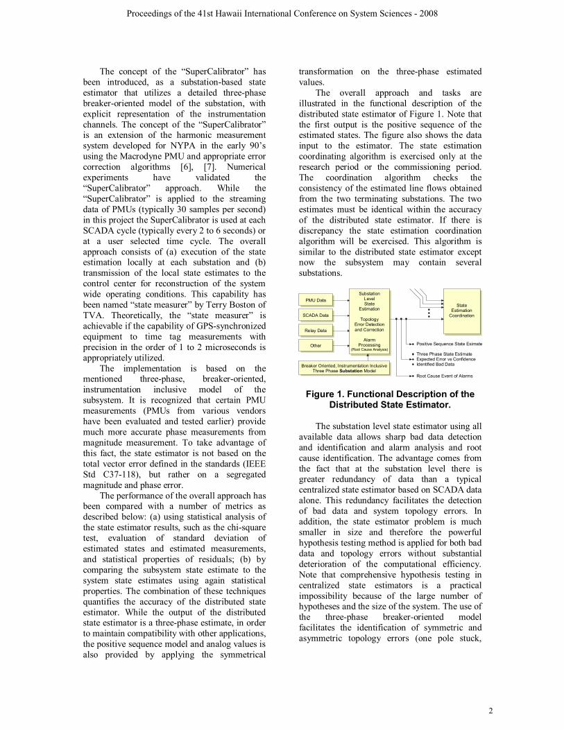
transformation on the three-phase estimated values. The overall approach and tasks are illustrated in the functional description of the distributed state estimator of Figure 1. Note that the first output is the positive sequence of the estimated states. The figure also shows the data input to the estimator. The state estimation coordinating algorithm is exercised only at the research period or the commissioning period. The coordination algorithm checks the consistency of the estimated line flows obtained from the two terminating substations. The two estimates must be identical within the accuracy of the distributed state estimator. If there is discrepancy the state estimation coordination algorithm will be exercised. This algorithm is similar to the distributed state estimator except now the subsystem may contain several substations.

PMU Data

SCADA Data

Relay Data

Other

SubstationLevelState

Estimation

TopologyError Detectionand Correction

Alarm Processing

(Root Cause Analysis)

Breaker Oriented, Instrumentation InclusiveThree Phase Substation Model

StateEstimation

Coordination

Positive Sequence State Esimate

Three Phase State EstimateExpected Error vs ConfidenceIdentified Bad Data

Root Cause Event of Alarms

Figure 1. Functional Description of the

Distributed State Estimator. The substation level state estimator using all available data allows sharp bad data detection and identification and alarm analysis and root cause identification. The advantage comes from the fact that at the substation level there is greater redundancy of data than a typical centralized state estimator based on SCADA data alone. This redundancy facilitates the detection of bad data and system topology errors. In addition, the state estimator problem is much smaller in size and therefore the powerful hypothesis testing method is applied for both bad data and topology errors without substantial deterioration of the computational efficiency. Note that comprehensive hypothesis testing in centralized state estimators is a practical impossibility because of the large number of hypotheses and the size of the system. The use of the three-phase breaker-oriented model facilitates the identification of symmetric and asymmetric topology errors (one pole stuck,


2

etc.). The traditional symmetric state estimators cannot identify asymmetric root cause events. It is important to recognize that the next generation of substations will have standards such as the IEC 61850, which will make available all the data from relays, PMUs, SCADA, meters, etc on a common bus accessible from any other device. In this case the proposed system will simply access the 61850 bus to retrieve the data and perform the estimation. 3. Distributed State Estimation Formulation This section presents an overview of the basic building blocks of the distributed state estimator. Detailed description of all the blocks is given in subsequent sections. 3.1. Basic Building Blocks The basic building blocks are:

1. The three-phase breaker-oriented power system model

2. The intelligent electronic device (RTU, relay, meter, disturbance recorder, PMU) with instrumentation model

3. The substation level static state estimation method

4. The substation level dynamic state estimation method

A brief description of each of these blocks is given below. Three-Phase Breaker-Oriented Model: Two sources of errors and biases for present-day state estimators are (a) system imbalances and (b) system asymmetries. These sources can be alleviated by using a three-phase breaker oriented model for the power system. And in particular, we use a physically based model from which the three-phase breaker-oriented model is extracted. The physically based model is a three dimensional model of the system inputted with a variety of user interfaces. Once the physical model is entered the mathematical model of the three-phase breaker oriented model is automatically constructed. This eliminates or minimizes human error in the construction of the model. IEDs/PMUs and Instrumentation Channel Model: An important issue is the accuracy of the available data. Specifically, GPS-synchronized equipment (PMUs) is in general higher precision equipment as compared

to typical SCADA systems. Conceptually, PMUs provide measurements that are time tagged with precision better than 1 microsecond and magnitude accuracy that is better than 0.1%. This potential performance is not achieved in an actual field installation because of two reasons: (a) different vendors use different design approaches that result in variable performance among vendors, for example use of multiplexing among channels or variable time latencies among manufacturers result in timing errors much greater than one microsecond, and (b) GPS-synchronized equipment receives inputs from instrument transformers, control cables, attenuators, etc. which introduce magnitude and phase errors that are much greater than the accuracy of PMUs. For example, many utilities may use CCVTs for instrument transformers. We refer to the errors introduced by instrument transformers, control cables, attenuators, etc. as the instrumentation channel error. The end result is that “raw” phasor data from different vendors cannot be used as highly accurate data. Conceptually, the overall precision issue can be resolved with sophisticated calibration methods. This approach is quite expensive and faces difficult technical problems. Specifically, it is extremely difficult to calibrate instrument transformers and the overall instrumentation channel in the field. Laboratory calibration of instrument transformers is possible, but a very expensive proposition, if not all, of instrument transformers need to be calibrated. In the early 90's the authors directed a research project in which we developed calibration procedures for selected NYPA’s high voltage instrument transformers [20]. From the practical point of view, this approach is an economic impossibility. An alternative approach is to utilize appropriate filtering techniques for the purpose of correcting the magnitude and phase errors, assuming that the characteristics of the various GPS-synchronized pieces of equipment are known and the instrumentation feeding this equipment is also known. We propose a viable and practical approach to correct for errors from instrumentation. Specifically, the models of the IEDs, PMUs and the associated instrumentation channel model is all integrated into a single model that provides the transfer function from the high voltage side to the output of the IEDs and PMUs. This model is also integrated with the three-phase breaker-oriented model that was described earlier. The end result is an accurate representation of the


3

physical system by which the measurements are taken. Substation Level Static State Estimation: The static state estimation algorithm utilizes the integrated model of the three-phase breaker-oriented instrumentation channel inclusive model and the set of measurements (excluding frequency and rate of change of frequency) to perform a state estimation, bad data detection and identification, topology error detection and identification for the purpose of extracting the real time model of the system. The overall mathematical process is assisted with a number of pseudomeasurements. Substation Level Dynamic State Estimation: The dynamic state estimation algorithm utilizes the integrated model of the three-phase breaker-oriented instrumentation channel inclusive model and the set of measurements (including frequency and change of frequency) to perform a state estimation, bad data detection and identification, topology error detection and identification for the purpose of extracting the real time model of the system. In this paper we focus on the substation level static state estimator. 3.2. State and Measurement Set The distributed state estimator takes advantage of the existing GPS-synchronized measurements for the purpose of partitioning the state estimator in an arbitrary manner. Specifically, for practical purposes the state estimation is defined at the substation level. Consider for example a substation as it is illustrated in Figure 2. The substation is connected to four other substations. The state estimation problem is defined for the network that is included within the boundaries of the substation and the interconnecting lines. The state that needs to be evaluated is the state of the substation only. For reasons of developing the simplest possible implementation we also include the voltage variables at the other end of the transmission lines. However the evaluation of these state variables is performed via pseudo-measurements for the purpose of avoiding the requirement of obtaining and transmitting via communication channels measurements from other substations.

Substation

V1e~ V2e

~

V3e~

V4e~

V1s~

V2s~

Figure 2. State Definition at Substation

Level. States within the substation: ss VandV 21

~,~.

States outside the substation:

eeee VandVVV 4321~,~,~,~

. Note that each one of the above states is a 4x1 complex vector as follows:

=

ns

cs

bs

as

s

VVVV

V

,1

,1

,1

,1

1

~~~~

~ ,

=

ns

cs

bs

as

s

VVVV

V

,2

,2

,2

,2

2

~~~~

~ ,

=

ne

ce

be

ae

e

VVVV

V

,1

,1

,1

,1

1

~~~~

~

,

=

ne

ce

be

ae

e

VVVV

V

,2

,2

,2

,2

2

~~~~

~

,

=

ne

ce

be

ae

e

VVVV

V

,3

,3

,3

,3

3

~~

~

~

,

=

ne

ce

be

ae

e

VVVV

V

,4

,4

,4

,4

4

~~~~

~ .

Measurements: The measurements utilized in this approach are all available measurements in the substation mainly from SCADA, Relays, IEDs, fault disturbance recorders and PMUs. The measurements are categorized into GPS-synchronized and non-synchronized ones. Mathematically these two categories are treated differently. The GPS-synchronized phasor measurement set consists of voltage and current measurements, both magnitude and phase in all three phases. Voltage measurements are direct state measurements. Current measurements can be expressed in terms of linear measurement equations with respect to the system state,


4

provided that a rectangular coordinate formulation is used. Non-synchronized measurements consist of SCADA measurements of voltage and, possibly, current magnitude, active and reactive power flows at each side of the substation transformer and on the substation end of the lines. Such measurements are typically obtained via analog measurement devices and are in general related to the system state via a set of non-linear equations. In our formulation such measurement equations are of degree at most quadratic. In addition to the actual measurements the approach is facilitated by a number of pseudomeasurements. These are defined below. Pseudomeasurements of the voltages at other end of lines (neighboring substations): These pseudo measurements are illustrated in

Figure 3. Given measurements of SV~ (all three

phases) and SI~ (all three phases) of a line i at a

substation k and a 3-phase model of the line, of the generalized pi-equivalent form:

=

R

S

R

S

VV

YYYY

II

~~

~~

2221

1211

Then the voltage pseudomeasurement at the other end of the line (neighboring substation) is defined by:

( ) ( ) SS

mpseudo

VYZYZIZYZ

VR

~~

~

21221

2222211

2222

,

−− −+−

=

II,

where 1

2221

1211

2221

1211−

=

YYYY

ZZZZ

and I is

the identity matrix of appropriate dimension.

Substation k

IS~

IR~

VS~

VR~

Line i

Figure 3. Pseudo-measurements of Voltage at Other End of Lines.

Pseudomeasurements from Kirchoff’s current law: These pseudomeasurements are

illustrated in Figure 4. In general it holds that

,0~ =∑ Ik where k is the voltage level ( kV level), at each internal note of the substation. Therefore, for the substation shown in Figure 4, the following equations define pseudomeasurements:

0~~~621 =++ III

Three equations, one for each phase

0~~~543 =++ III


( ) ( ) 0~~~~~212431 =++++ mIIIkIIk


mI~ is the transformer magnetizing current. Since its value is rather small, it can be neglected without significant loss of accuracy. The coefficients 1k and 2k are the two voltage levels that define the transformation ratio of the power transformer.

Substation

I4~

I3~

I5~

I6~

I1~

I2~

Figure 4. Pseudo-measurements from Kirchoff’s Current Law.

Pseudo-measurements of the individual phase voltages: These pseudo measurements are introduced if the measurement of a single phase is missing or is not available. Assuming that phase A voltage measurement exists, while phase C voltage measurement does not. In this case the following equation is introduced, defining a pseudo-measurement equation for phase C:

0

/

240, ~~ ja

mpseudo eVVns

−= or

0~~ 0

/

240, =− − ja

mpseudo eVVns

Pseudomeasurements of the neutral/shield wire current: These pseudo measurements are introduced as follows:


5

s/nabc

Figure 5. Pseudo-measurements from Neutral/Shield Wire Current.

Given a line model we can compute the ratio of shield/neutral current over the return current as:

( )cba

ns

IIII

~~~~

/

++−=α .

Then the following pseudomeasurement is introduced:

( )cbampseudo IIII

ns

~~~~ ,/

++−= α or

( ) 0~~~~ ,/

=+++ cbampseudo IIII

nsα .

Pseudomeasurements of the neutral/ground voltage: The neutral/ground voltage is computed as the product of the substation ground impedance and the earth current. The earth current is the sum of all earth currents of all transmission lines connected to the substation. The equations are:

( )( )∑ ++−−=i

icibiaigmpseudo

nS IIIRV ,,,, ~~~1~ α

where gR is the substation ground resistance and the coefficient a is the ratio of shield/neutral current over the return current. Note that under normal operating conditions the neutral/ground voltage will be negligibly small. However during a fault condition or a stuck breaker the neutral/ground voltage may be elevated to a substantial value. 3.2. Instrumentation Model PMUs, SCADA, relaying, metering and disturbance recording use a system of instrument transformers to scale the power system voltages and currents into instrumentation level voltages and currents. Standard instrumentation level voltages and currents are 67V or 115V and 5A respectively. These standards were established many years ago to accommodate the electromechanical relays. Today, the instrument transformers are still in use, but because modern relays, metering and disturbance recording operates at much lower voltages, it is necessary

to apply another transformation from the previously defined standard voltages and currents to another set of standard voltages of 10V or 2V. This means that the modern instrumentation channel consists of typically two transformations and additional wiring and possibly burdens. Figure 6 illustrates typical instrumentation channels, a voltage channel and a current channel. Phase Conductor

PotentialTransformer

CurrentTransformer

PhasorMeasurementUnit

ComputerBurden

InstrumentationCables

v(t)

v1(t) v2(t)

v3(k)

Burdeni2(t)i1(t)

i(t)

Attenuator

Attenuator

Figure 6. Typical Instrumentation Channel for Data Collection.

Note that each component of the instrumentation channel will introduce an error. Of importance is the net error introduced by all the components of the instrumentation channel. The overall error can be defined as follows. Let the voltage or current at the power system be:

)(),( titv aa An ideal instrumentation channel will generate a waveform at the output of the channel that will be an exact replica of the waveform at the power system. If the nominal transformation ratio is kv and ki for the voltage and current instrumentation channels respectively, then the output of the ideal channels will be:

)()(),()( tiktitvktv aiidealavideal == The error is defined as follows:

)()()(),()()(

titititvtvtv

idealouterror

idealouterror

−=−=

where the subscript “out” refers to the actual output of the instrumentation channel. The error waveform can be analyzed to provide the rms value of the error, the phase error, etc. The overall instrumentation channel error can be characterized with the gain function of the entire channel defined with (for voltage and current measurement respectively):

( ) ( )( ) ( ) ( )

( )fIfI

fgandfVfV

fgin

outij

in

outvj ~

~~~

,, ==

The instrumentation error can be computed by appropriate models of the entire


6

instrumentation channel. It is important to note that some components may be subject to saturation (CTs and PTs), while other components may include resonant circuits with difficult to model behavior (CCVTs). In general it is straightforward to model the instrumentation channel and compute the transfer function. Then the transfer function is integrated into the state estimation model. 3.3. Distributed State Estimator Algorithm The formulation is presented with the following postulated model:

η+= )(xz h where z is a vector of three phase measurements; x is a vector of the state (three-phase state); η is a vector of error; h is a vector function depending on the system modeling. The three-phase state estimator is formulated by selecting the three-phase state, the three-phase measurements and the three-phase system model. These are described next. The hybrid estimation process minimizes the following objective function which includes all the available measurement data:

∑∑−∈∈

+=synnonphasor

JMinν ν

νν

ν ν

νν

σηη

σηη

22

* ~~

It is noted that if all measurements are synchronized, the state estimation problem becomes linear and the solution is obtained directly. In the presence of non-synchronized measurements and in terms of the above formulation, the problem can be made quadratic. Specifically, using the quadratic formulation, the measurements can be separated into phasor and non-synchronized measurements with the following form:

sss xHz η+=

{ } niT

nn xQxxHz η++=

In the above equations, the subscript s indicates phasor measurements while the subscript n indicates non-synchronized measurements. The best state estimate is given by: Case 1: Phasor measurements only.

( ) sTss

Ts WzHWHHx 1ˆ −=

Case 2: Phasor and non-synchronized measurements.

( ) { }

−−

−+=

−+ννν

ννν

xQxxHzxHz

WHWHHxxinn

ssTTT

ˆˆˆˆ

ˆˆ 11

where:

=

n

s

WW

W0

0

and

+

=qnn

s

HHH

H.

4. Quantification of SuperCalibrator Output Accuracy The overall accuracy and performance of the SuperCalibrator can be evaluated using the concept of the confidence level as in the case of the traditional state estimator. Again one has to identify the number of states, the number of measurements for the purpose of computing the degrees of freedom. Then at the state estimate, the value of the objective function should be computed. More specifically, with respect to the quality of state estimation, there are two related problems. The first one relates to the validity of the data (measurements). If the measurements are polluted with reasonable measurement error (within the specifications of the measuring instruments), and assuming there is enough redundancy, the state estimate will be reasonably accurate. However, if one or more data have large errors (due to a number of reasons), the state estimate will not be accurate. Thus, it is necessary that the state estimator be able to detect and reject bad data. The second problem relates to the error transmitted to the state estimate from the measurement error. This error is measured with the standard deviation of the state estimate. It should be expected that in the presence of statistically reasonable measurement errors, the standard deviation of the state estimate should decrease as the redundancy increases. Consider a measurement of a physical quantity of an electric power system. We have discussed the fact that this measurement is obtained via an instrumentation channel that can be complex. The measurement process will exhibit some error. For simplicity, we introduced a number of assumptions regarding the measurement error. Consider the normalized error for measurement i, is :

i

iii

bhs

σ−

=)(x

,


7

where )(xih is the measurement model, ib the

measurement value and iσ the standard deviation of the measurement. It is assumed that the normalized errors are Gaussian distributed with standard deviation 1.0 and zero cross correlation. Given the meter accuracy defined above, two problems can be defined as follows: (a) what is the probability that all data are located within expected bounds (goodness of fit) and (b) what is the accuracy of the computed solution. These problems will be addressed next. Te approach is the same statistical approach as in the traditional state estimation, therefore the description will be brief. Goodness of Fit: The goodness of fit is defined as the probability that the distribution of the measurement errors are within the expected bounds. This probability is computed via standard hypothesis testing, using the chi-square distribution, with nm − degrees of freedom, of the normalized measurement residuals. m is the total number of measurements, n is the number of estimated state variables. Solution Accuracy: The accuracy of the solution is expressed with the covariance matrix of the state estimate, x̂ . Specifically, let x be the true, but unknown, solution, and x̂ be the solution to the least squares problem. The definition of the covariance matrix is:

])ˆ)(ˆ[( Tx EC xxxx −−=

Note that a linearized expression for xx −ˆ is as follows (which is obtained by applying the state estimation algorithm at point x )

WrHWHH TT 1)(ˆ −=− xx (for least square solution ) where bhr −= )(x and H is the Jacobian matrix of the measurement equations. The Jacobian is supposed to be computed at the true state x . However, since the true state is not known, we approximate the Jacobian matrix at the known best estimate of the state, x̂ . As we discussed, the residuals r represent the measurement errors, i.e. η=r . The statistics of the measurement error are 0][ =ηE and

1][ −= WE Tηη . Upon substitution of above into the definition of the covariance matrix, the following is obtained

])()[( 1 TTTTTTx WHHHWWHWHHEC −−= ηη

and the above equation is simplified to yield:

1)( −= WHHC Tx

Once the covariance matrix of the solution has been computed, the standard deviation of a component of the solution vector x is given with

),( iiCxxi=σ

where, ),( iiCx is the ith diagonal entry of the covariance matrix. In summary, the quality of the state estimate is quantified as follows: A measure of data validity is expressed with the confidence level obtained from the chi-square distribution. The accuracy of the estimated state variables is given with the diagonal entries of the information matrix which express the square of the standard deviation. 5. Implementation and Demonstration Projects The distributed state estimator was demonstrated on two subsystems, each subsystem comprised two substations. The approach described in this report has been implemented to two systems of two substations each interconnected with a transmission line. The systems are: The MARCY and MESSINA substations of the New York Power Authority (NYPA) system, and The PANAMA and ROMEVILLE substation of the Entergy system. These two test systems consist of two interconnected substations each. Figure 7 illustrates the NYPA test system, while Figure 8 illustrates the Entergy test system.

Figure 7. One-Line Diagram of NYPA Test System Superimposed on NY State Map.


8

SUB

PANAMA

SUB

ROMEVILLE

PANROM

ROM-PAN-L

Figure 8. One-Line Diagram of Entergy

Test System Superimposed on an Aerial Picture of the Area.

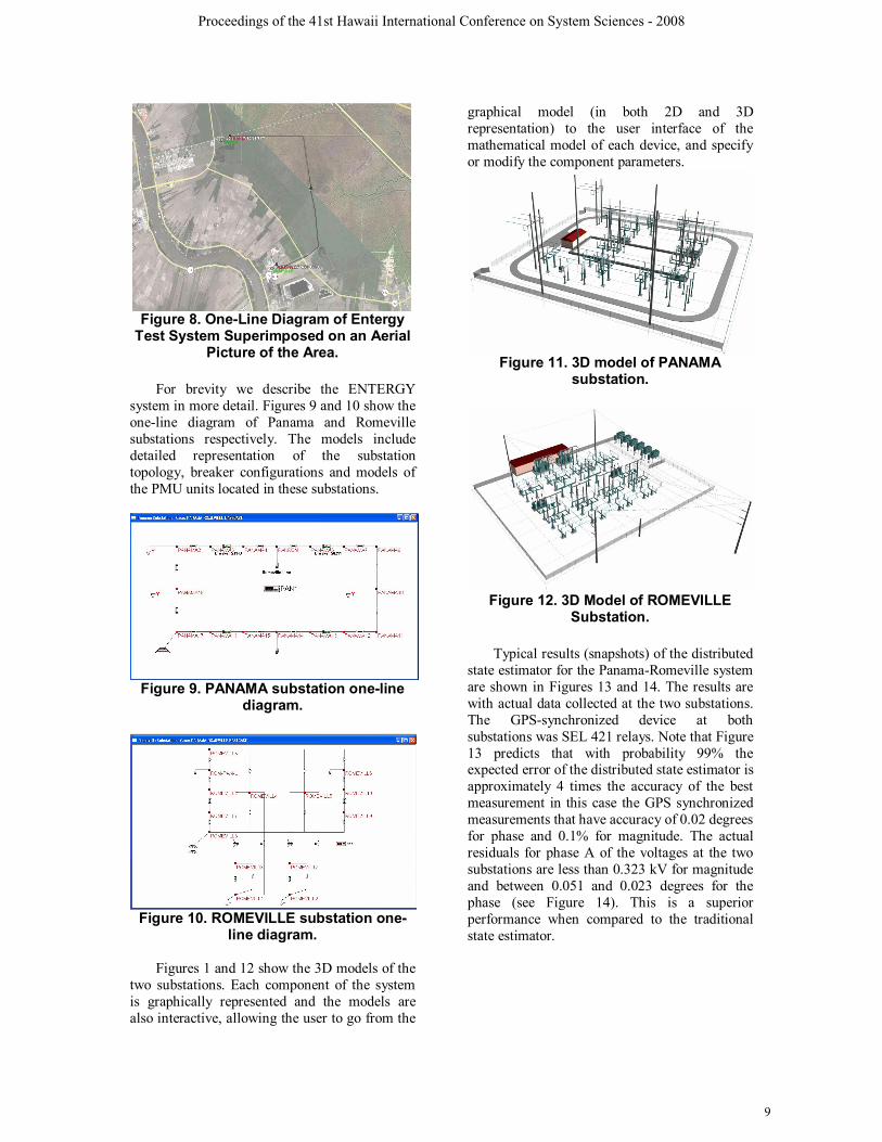
For brevity we describe the ENTERGY system in more detail. Figures 9 and 10 show the one-line diagram of Panama and Romeville substations respectively. The models include detailed representation of the substation topology, breaker configurations and models of the PMU units located in these substations.

Figure 9. PANAMA substation one-line

diagram.

Figure 10. ROMEVILLE substation one-

line diagram. Figures 1 and 12 show the 3D models of the two substations. Each component of the system is graphically represented and the models are also interactive, allowing the user to go from the

graphical model (in both 2D and 3D representation) to the user interface of the mathematical model of each device, and specify or modify the component parameters.

Figure 11. 3D model of PANAMA

substation.

Figure 12. 3D Model of ROMEVILLE

Substation. Typical results (snapshots) of the distributed state estimator for the Panama-Romeville system are shown in Figures 13 and 14. The results are with actual data collected at the two substations. The GPS-synchronized device at both substations was SEL 421 relays. Note that Figure 13 predicts that with probability 99% the expected error of the distributed state estimator is approximately 4 times the accuracy of the best measurement in this case the GPS synchronized measurements that have accuracy of 0.02 degrees for phase and 0.1% for magnitude. The actual residuals for phase A of the voltages at the two substations are less than 0.323 kV for magnitude and between 0.051 and 0.023 degrees for the phase (see Figure 14). This is a superior performance when compared to the traditional state estimator.


9

ENTERGY: Panama-Romeville 230 kV Line - Dynamic Rating project

100m 1 10 100Confidence Level (%)

1

10

Para

met

er k

Error Parameter Versus Confidence Level

Case :

State Estimation Solution Report

Status : Solution Completed

4.274 99.00

12 degrees of freedomProgram WinIGS-F - Form QPFSE_GEN_REPORT Figure 13. Results of chi-Square Test for One Snapshot of the Distributed State Estimator

Figure 14. Visualization of Voltage Magnitude

and Phase Residuals Amplified by 300 for Phase and by 20 for Magnitude

6. Conclusions This paper presented recent work and advances in the SuperCalibrator concept. The complexity of state estimation using the SuperCalibrator approach appears to be significantly higher, compared to the traditional state estimation, however, there are significant advantages that fully justify the approach. Compared to more traditional state estimation approaches the SuperCalibrator presents the following advantages: • Utilization of full three-phase system models:

More accurate system modeling results in more realistic and accurate measurement equations and thus more precise estimation results. Such a modeling can capture system imbalances that frequently occur, even at the transmission level as well as system asymmetries.

• Inclusion of instrumentation channel modeling: Instrumentation channels may play an important role in the accuracy of the data and can introduce significant errors. Their modeling can eliminate most of such errors via software.

• Utilization of all available data: In the presented approach all data at the substation level coming from various measuring devices are utilized and included in the estimation process. Such data can come from PMUs, relays, other IEDs or the SCADA system and can be either synchronized of not. Therefore, the estimate is more accurate and the redundancy of measurements increases dramatically. Furthermore, no data that are already available are “wasted” by being ignored in the state estimation algorithm.

• Distributed SE approach: The SuperCalibrator concept operates on all available (static and streaming) data at the substation level. Only data obtained locally are utilized, therefore minimizing communication burden and latencies as well as computational burden.

• Quantification of data accuracy: The output of the algorithm also quantifies the data accuracy; thus is can be used to remotely calibrate the measuring system. This is also where the name SuperCalibrator came from.

• Minimization of transferred data: This is a very important advantage of SuperCalibrator. Since all the computations are performed locally, on a distributed basis, and also only local data are used significant improvements can be achieved in terms of communication latencies. Only the results of the local estimation need to be communicated, therefore we have only communication of information and not raw data. The amount of data of the estimation results at each substation is orders of magnitude less than the amount of available row data.

7. Acknowledgments The work reported in this paper has been supported by the CTC project “Distributed State Estimation”. This support is gratefully acknowledged. 8. References [1] D. M. Falcao, F. F. Wu, L. Murphy, “Parallel and

distributed state estimation,” IEEE Transactions


10

on Power Systems, vol 10, No 2, pp 724-730, May 1995.

[2] R. Ebrahimian, R. Baldick, “State estimation distributed processing [for power systems],” IEEE Transactions on Power Systems, vol 15, No 4, pp 1240-1246, Nov. 2000.

[3] Zhao Liang, A. Abur, “Multi area state estimation using synchronized phasor measurements,” IEEE Transactions on Power Systems, vol 20, No 2, pp 611-617, May 2005.

[4] M. M. Nordman, M. Lehtonen, “Distributed agent-based state estimation for electrical distribution networks,” IEEE Transactions on Power Systems, vol 20, No 2, pp 652-658, May 2005.

[5] Yan Li, Xiaoxin Zhou, Jingyang Zhou, “A new algorithm for distributed power system state estimation based on PMUs,” Proceeding of the 2006 International Conference on Power System Technology (PowerCon 2006), Oct. 2006.

[6] A. P. Sakis Meliopoulos, F. Zhang, and S. Zelingher, 'Hardware and Software Requirements for a Transmission System Harmonic Measurement System', Proceedings of the 5th International Conference on Harmonics in Power Systems, ICHPS V, pp 330-338, Atlanta, GA, September 22-25, 1992.

[7] A. P. Sakis Meliopoulos, F. Zhang, and S. Zelingher, 'Power System Harmonic State Estimation,' IEEE Transactions on Power Systems, Vol. 9, No. 3, pp 1701-1709, July 1994.

[8] B. Fardanesh, S. Zelingher, A. P. Sakis Meliopoulos, G. Cokkinides and Jim Ingleson, ‘Multifunctional Synchronized Measurement Network’, IEEE Computer Applications in Power, Volume 11, Number 1, pp 26-30, January 1998.

[9] J. Chen, A. Abur, “Placement of PMUs to enable bad data detection in state estimation,” IEEE Transactions on Power Systems, vol 21, No 4, pp 1608-1615, Nov. 2006.

[10] Sakis Meliopoulos, “State Estimation for Mega RTOs,” Proceedings of the 2002 IEEE PES Winter Meeting, New York, NY, Jan 28-31, 2002.

[11] A. V. Jaen, P.C. Romero, and A. G. Exposito, “Substation data validation by a local three-phase generalized state estimator,” IEEE Transactions on Power Systems, vol 20, No 1, pp 264-271, Feb. 2005.

[12] A. P. Meliopoulos, G. J. Cokkinides, Floyd Galvan and Bruce Fardanesh, ”GPS-Synchronized Data Acquisition: Technology Assessment and Research Issues”, Proceedings of the of the 39st Annual Hawaii International Conference on System Sciences, Kaua’i, Hawaii, January 4-7, 2006.

[13] Jun Zhu, Ali Abur, Mark Rice and Gerald T. Heydt, Sakis Meliopoulos, “Enhanced state estimators,” Final project report for PSERC project S-22, Nov. 2006. Available at www.pserc.org

[14] Zhong Shan, A. Abur, “Effects of nontransposed lines and unbalanced loads on state estimation,” IEEE Power Engineering Society 2002 Winter Meeting, vol. 2, pp 975-979, Jan. 2002.

[15] A. P. Sakis Meliopoulos and George J. Cokkinides, “A Virtual Environment for Protective Relaying Evaluation and Testing”, IEEE Transactions of Power Systems, Vol. 19, No. 1, pp. 104-111, February, 2004.

[16] A. P. Sakis Meliopoulos and G. J. Cokkinides, ”Visualization and Animation of Instrumentation Channel Effects on DFR Data Accuracy”, Proceedings of the 2002 Georgia Tech Fault and Disturbance Analysis Conference, Atlanta, Georgia, April 29-30, 2002.

[17] T. K. Hamrita, B. S. Heck and A. P. Sakis Meliopoulos, ‘On-Line Correction of Errors Introduced By Instrument Transformers In Transmission-Level Power Waveform Steady-State Measurements’, IEEE Transactions on Power Delivery, Vol. 15, No. 4, pp 1116-1120, October 2000.

[18] A. P. Sakis Meliopoulos and George J. Cokkinides, “Virtual Power System Laboratories: Is the Technology Ready?”, Proceedings of the 2000 IEEE/PES Summer Meeting, Seattle, WA, July 16-20, 2000.

[19] A. P. Sakis Meliopoulos, George J. Cokkinides, “Visualization and Animation of Protective Relays Operation From DFR Data”, Proceedings of the 2001 Georgia Tech Fault and Disturbance Analysis Conference, Atlanta, Georgia, April 30-May 1, 2001.

[20] A. P. Meliopoulos, F. Zhang, S. Zelingher, G. Stillmam, G. J. Cokkinides, L. Coffeen, R. Burnett, J. McBride, 'Transmission Level Instrument Transformers and Transient Event Recorders Characterization for Harmonic Measurements,' IEEE Transactions on Power Delivery, Vol 8, No. 3, pp 1507-1517, July 1993.

[21] A. P. Sakis Meliopoulos and G. J. Cokkinides, ”Phasor Data Accuracy Enhancement in a Multi-Vendor Environment”, Proceedings of the 2005 Georgia Tech Fault and Disturbance Analysis Conference, Atlanta, Georgia, April 25-26, 2005

[22] Zhong Shan, A. Abur, “Combined state estimation and measurement calibration,” IEEE Transactions on Power Systems, vol 20, No 1, pp 458-465, Feb. 2005.

[23] A. P. Meliopoulos, G. J. Cokkinides, Floyd Galvan, Bruce Fardanesh and Paul Myrda, “Advances in the SuperCalibrator Concept – Practical Implementations,” Proceedings of the of the 40st Annual Hawaii International Conference on System Sciences, Kona, Hawaii, January 3-6, 2007.


11

Distributed State Estimator Advances and Demonstration

Documents

Transcript of Distributed State Estimator Advances and Demonstration