On the Grenander estimator at zero

ON THE GRENANDER ESTIMATOR AT ZERO

Fadoua Balabdaoui1, Hanna Jankowski2, Marios Pavlides3,Arseni Seregin4, and Jon Wellner4

1Universite Paris-Dauphine, 2York University, 3Frederick University Cyprusand 4University of Washington

Abstract: We establish limit theory for the Grenander estimator of a mono-

tone density near zero. In particular we consider the situation when the true

density f0 is unbounded at zero, with di!erent rates of growth to infinity. In

the course of our study we develop new switching relations by use of tools

from convex analysis. The theory is applied to a problem involving mixtures.

Key words and phrases: Convex analysis, inconsistency, limit distribution,

maximum likelihood, mixture distributions, monotone density, nonparametric

estimation, Poisson process, rate of growth, switching relations.

1. Introduction and Main Results

Let X1, . . . ,Xn be a sample from a decreasing density f0 on (0,!), and let!fn denote the Grenander estimator (i.e. the maximum likelihood estimator) off0. Thus !fn " !fL

n is the left derivative of the least concave majorant !Fn of theempirical distribution function Fn; see e.g. Grenander (1956a,b), Groeneboom(1985), and Devroye (1987, chapter 8).

The Grenander estimator !fn is a uniformly consistent estimator of f0 on setsbounded away from 0 if f0 is continuous:

supx!c

| !fn(x) # f0(x)| $a.s. 0

for each c > 0. It is also known that !fn is consistent with respect to the L1 (%p#q%1 "

"|p(x) # q(x)|dx) and Hellinger (h2(p, q) " 2"1

" #$p(x) #

$q(x)

%2dx)

metrics: that is,

% !fn # f0%1 $a.s. 0 and h( !fn, f0) $a.s. 0;

see e.g. Devroye (1987, Theorem 8.3, page 144) and van de Geer (1993).1

2 BALABDAOUI, JANKOWSKI, PAVLIDES, SEREGIN, WELLNER

However, it is also known that !fn(0) " !fn(0+) is an inconsistent estimatorof f0(0) " f0(0+) = limx#0 f0(x), even when f0(0) < !. In fact, Woodroofeand Sun (1993) showed that

!fn(0) $d f0(0) supt>0

N(t)t

d= f0(0)1U

(1.1)

as n $ ! where N is a standard Poisson process on [0,!) and U & Uniform(0, 1).Woodroofe and Sun (1993) introduced penalized estimators &fn of f0 which yieldconsistency at 0: &fn(0) $p f0(0). Kulikov and Lopuhaa (2006) study estimationof f0(0) based on the Grenander estimator !fn evaluated at points of the form t =cn"! . Among other things, they show that !fn(n"1/3) $p f0(0) if |f $

0(0+)| > 0.Our view in this paper is that the inconsistency of !fn(0) as an estimator of

f0(0) exhibited in (1.1) can be regarded as a simple consequence of the fact thatthe class of all monotone decreasing densities on (0,!) includes many densitiesf which are unbounded at 0, so that f(0) = !, and the Grenander estimator!fn simply has di!culty deciding which is true, even when f0(0) < !. From thisperspective we would like to have answers to the following three questions undersome reasonable hypotheses concerning the growth of f0(x) as x ' 0:

Q1: How fast does !fn(0) diverge as n $ !?

Q2: Do the stochastic processes {bn!fn(ant) : 0 ( t ( c} converge for some

sequences an, bn, and c > 0?

Q3: What is the behavior of the relative error

sup0%x%cn

''''!fn(x)f0(x)

# 1''''

for some constant cn?

It turns out that answers to questions Q1 - Q3 are intimately related to thelimiting behavior of the minimal order statistic Xn:1 " min{X1, . . . ,Xn}. ByGnedenko (1943) or de Haan and Ferreira (2006, Theorem 1.1.2, page 5)), it iswell-known that there exists a sequence {an} such that

a"1n Xn:1 $d Y(1.2)

where Y has a nondegenerate limiting distribution G if and only if

nF0(anx) $ x! , x > 0,(1.3)

GRENANDER ESTIMATOR AT ZERO 3

for some ! > 0, and hence an $ 0. One possible choice of an is an = F"10 (1/n),

but any sequence {an} satisfying nF0(an) $ 1 also works. Since F0 is concavethe convergence in (1.3) is uniform on any interval [0,K]. Concavity of F0 andexistence of f0 also implies convergence of the derivative:

nanf0(anx) $ !x!"1.(1.4)

By Gnedenko (1943), (1.2) is equivalent to

limx&0+

F0(cx)F0(x)

= c! , c > 0.(1.5)

Thus (1.2), (1.3), and (1.5) are equivalent. In this case we have:

G(x) = 1 # e"x!

, x ) 0.(1.6)

Since F0 is concave, the power ! * (0, 1].As illustrations of our general result, we consider the following three hy-

potheses on f0:

G0: The density f0 is bounded at zero: f0(0) < !.

G1: For some " ) 0 and 0 < C1 < !,

(log(1/x))""f0(x) $ C1 as x ' 0.

G2: For some 0 ( # < 1 and 0 < C2 < !

x#f0(x) $ C2 as x ' 0.

Note that in G2 the value # = 1 is not possible for a positive limit C2 sincexf(x) $ 0 as x $ 0 for any monotone density f ; see e.g. Devroye (1986,Theorem 6.2, page 173). Below we assume that F0 satisfies the condition (1.5).Our cases G0 and G1 correspond to ! = 1 and G2 to ! = 1 # #.

One motivation for considering monotone densities which are unboundedat zero comes from the study of mixture models. An example of this type, asdiscussed by Donoho and Jin (2004), is as follows. Suppose X1, . . . ,Xn are i.i.d.with distribution function F where,

under H0 : F = ", the standard normal d.f.

under H1 : F = (1 # $)"+ $"(·# µ), $ * (0, 1), µ > 0.


If we transform to Yi " 1 # "(Xi) & G, then, for 0 ( y ( 1,

under H0 : G(y) = y, the Uniform(0, 1) d.f.,

under H1 : G = G$,µ(y) = (1 # $)y + $(1 # "(""1(1 # y) # µ)).

It is easily seen that the density g$,µ of G$,µ, given by

g$,µ(y) = (1 # $) + $%(""1(1 # y) # µ)%(""1(1 # y))

,

is monotone decreasing on (0, 1) and is unbounded at zero. As we will show inSection 4, G$,µ satisfies our key hypothesis (1.5) below with ! = 1. Moreover,we will show that the whole class of models of this type with " replaced by thegeneralized Gaussian (or Subbotin) distribution, also satisfy (1.5), and hence thebehavior of the Grenander estimator at zero gives information about the behaviorof the contaminating component of the mixture model (in the transformed form)at zero.

Another motivation for studying these questions in the monotone densityframework is to gain insights for a study of the corresponding questions in thecontext of nonparametric estimation of a monotone spectral density. In that(related, but di#erent) setting, singularities at the origin correspond to the in-teresting phenomena of long-range dependence and long-memory processes; seee.g. Cox (1984), Beran (1994), Martin and Walker (1997), Gneiting (2000), andMa (2002). Although our results here do not apply directly to the problem ofnonparametric estimation of a monotone spectral density function, it seems plau-sible that similar results will hold in that setting; note that when f is a spectraldensity, the assumptions G1 and G2 correspond to long-memory processes (withthe usual description being in terms of " = 1## * (0, 1) or the Hurst coe!cientH = 1 # "/2 = 1 # (1 # #)/2 = (1 + #)/2). See Anevski and Soulier (2009) forrecent work on nonparametric estimation of a monotone spectral density.

Let N denote the standard Poisson process on R+. When (1.5) and hencealso (1.6) hold, it follows from Miller (1976, Theorem 2.1, page 522) togetherwith Jacod and Shiryaev (2003, Theorem 2.15(c)(ii), pages 306-307), that

nFn(ant) + N(t!) in D[0,!),(1.7)

which should be compared to (1.3).


Since we are studying the estimator !fn near zero and because the valueof !fn at zero is defined as the right limit limx#0

!fn(x) " !fn(0), it is sensible tostudy instead the right-continuous modification of !fn, and this of course coincideswith the right derivative !fR

n of the least concave majorant !Fn of the empiricaldistribution function Fn. Therefore we change notation for the rest of this paperand write !fn for !fR

n throughout the following. We write !fLn for the left-continuous

Grenander estimator.We now obtain the following theorem concerning the behavior of the Grenan-

der estimator at zero.

Theorem 1.1. Suppose that (1.5) holds. Let an satisfy nF0(an) & 1, let !h!

denote the right derivative of the least concave majorant of t ,$ N(t!), t ) 0.Then:(i) nan

!fn(tan) + !h!(t) in D[0,!).(ii) For all c ) 0

sup0<x%can

'''''!fn(x)f0(x)

# 1

''''' $d sup0<t%c

'''''t1"!!h!(t)

!# 1

''''' .

The behavior of !fn near zero under the di#erent hypotheses G0, G1, andG2 now follows as corollaries to Theorem 1.1. Let Y! " !h!(0). We then have

Y! = supt>0

(N(t!)/t) = sups>0

(N(s)/s1/!).(1.8)

Here we note that Y1 =d 1/U where U & Uniform(0, 1) has distribution functionH1(x) = 1 # 1/x for x ) 1. The distribution of Y! for ! * (0, 1] is given inProposition 1.5 below. The first part of the following corollary was establishedby Woodroofe and Sun (1993).

Corollary 1.2. Suppose that G0 holds. Then ! = 1, a"1n = nf0(0+) satisfies

nF0(an) $ 1, and it follows that:(i)

!fn(0) $d f0(0)!h1(0) = f0(0)Y1.

(ii) The processes {t ,$ !fn(tn"1) : n ) 1} satisfy

!fn(tn"1) + f0(0)!h1(f0(0)t) in D[0,!).


(iii) For cn = c/n with c > 0,

sup0<x%cn

'''''!fn(x)f0(x)

# 1

''''' $d Y1 # 1

which has distribution function H1(x + 1) = 1 # 1/(x + 1) for x ) 0.

Corollary 1.3. Suppose that G1 holds. Then F0(x) & C1x(log(1/x))" , so ! = 1,and a"1

n = C1n(log n)" satisfies nF0(an) $ 1. It follows that:(i)

!fn(0)(log n)"

$d C1Y1.

(ii) The processes {t ,$ (log n)"" !fn(t/(n(log n)")) : n ) 1} satisfy

1(log n)"

!fn

(t

n(log n)"

)+ C1

!h1(C1t) in D[0,!)

(iii) For cn = c/(n(log n)") with c > 0,

sup0<x%cn

'''''!fn(x)f0(x)

# 1

''''' $d Y1 # 1.

Corollary 1.4. Suppose that G2 holds and set &C2 = (C2/(1# #))1/(1"#). ThenF0(x) & C2x1"#/(1 # #), so ! = 1# #, a"1

n = &C2n1/(1"#) satisfies nF0(an) $ 1,and it follows that:(i)

!fn(0)n#/(1"#)

$d&C2Y1"#.(1.9)

(ii) The processes {t ,$ n"#/(1"#) !fn(tn"1/(1"#)) : n ) 1} satisfy!fn(tn"1/(1"#))

n#/(1"#)+ &C2

!h1"#( &C2t) in D[0,!).

(iii) For cn = c/n1/(1"#) with c > 0,

sup0<x%cn

'''''!fn(x)f0(x)

# 1

''''' $d sup0<t%c eC2

'''''t#!h1"#(t)

1 # ## 1

''''' .

Taking " = 0 in (i) of Corollary 1.3 yields the limit theorem (1.1) of Woodroofeand Sun (1993) as a corollary; in this case C1 = f0(0). Similarly, taking # = 0 in(ii) of Corollary 1.4 yields the limit theorem (1.1) of Woodroofe and Sun (1993)


as a corollary; in this case C2 = f0(0). Note that Theorem 1.1 yields furthercorollaries when assumptions G1 and G2 are modified by other slowly varyingfunctions.

Recall the definition (1.8) of Y! . The following proposition gives the distri-bution of Y! for ! * (0, 1].

Proposition 1.5. For fixed 0 < ! ( 1 and x > 0,

Pr(

sups>0

*N(s)s1/!

+( x

)=

,1 # 1/x , if ! = 1, x ) 1,1 #

-'k=1 ak(x, !) , if ! < 1, x > 0,

where the sequence {ak(x, !)}k!1 is constructed recursively as follows:

a1(x, !) = p

((1x

)!

; 1)

,

and, for j ) 1,

ak(x, !) = p

((k

x

)!

; k)#

k"1.

i=1

*ai(x, !) · p

((k

x

)!

#(

i

x

)!

; k # i

)+,

where p(m; k) " e"mmk/k!.

0 2 4 6 8 10

0.00.2

0.40.6

0.81.0

gamma=1.0gamma=0.8gamma=0.6gamma=0.4gamma=0.2

Figure 1. The distribution functions of Y!, ! * {0.2, 0.4, 0.6, 0.8, 1.0}.


Remark 1.6. The random variables Y! are increasingly heavy-tailed as ! de-creases; cf. Figure 1. Let T1, T2, . . . be the event times of the Poisson process N;i.e. N(t) =

-'j=1 1[Tj%t]. Then note that

Y!d= sup

j!1

j

T 1/!j

) 1

T 1/!1

where T1 & Exponential(1). On the other hand

Y! =(

supt>0

N(t)!

t

)1/!

((

supt>0

N(t)t

)1/!d=

1U1/!

where U & Uniform(0, 1). Thus it is easily seen that E(Y r! ) < ! if and only if

r < !, and that the distribution function F! of Y! is bounded above and below bythe distribution functions GL

! and GU! of 1/T 1/!

1 and 1/U1/! , respectively.

The proofs of the above results appear in Appendix A. They rely heavilyon a set equality known as the “switching relation”. We study this relationusing convex analysis in Section 2. Section 3 gives some numerical results whichaccompany the results presented here, and Section 4 studies applications to theestimation of mixture models.

2. Switching relations

In this section we consider several general variants of the so-called switchingrelation first given in Groeneboom (1985), and used repeatedly by other authors,including Kulikov and Lopuhaa (2005, 2006), and van der Vaart and Wellner(1996). Other versions of the switching relation were also studied by van derVaart and van der Laan (2006, Lemma 4.1). In particular, we provide a novelproof of the result using convex analysis. This approach also allows us to re-statethe relation without restricting the domain to compact intervals. Throughout thissection we make use of definitions from convex analysis (cf. Rockafellar (1970);Rockafellar and Wets (1998); Boyd et al. (2004)) which are given in AppendixB.

Suppose that " is a function, " : D $ R, defined on the (possibly infinite)closed interval D - R. The least concave majorant !" of " is the pointwiseinfimum of all closed concave functions g : D $ R with g ) ". Since !" isconcave, it is continuous on Do, the interior of D. Furthermore, !" has left


and right derivatives on Do, and is di#erentiable with the exception of at mostcountably many points. Let !%L and !%R denote the left and right derivatives,respectively, of !".

If " is upper semicontinuous, then so is the function "y(x) = "(x) # yx foreach y * R. If D is compact, then "y attains a maximum on D, and the setof points achieving the maximum is closed. Compactness of D was assumed byvan der Vaart and van der Laan (2006, see their Lemma 4.1, page 24). One ofour goals here is to relax this assumption.

Assuming they are defined, we consider the argmax functions

&L(y) " argmaxL"y " argmaxLx{"(x) # yx}

= inf{x * D : "y(x) = supz(D

"y(z)},

&R(y) " argmaxR"y " argmaxRx {"(x) # yx}

= sup{x * D : "y(x) = supz(D

"y(z)}.

Theorem 2.1. Suppose that " is a proper upper-semicontinuous real-valuedfunction defined on a closed subset D - R. Then !" is proper if and only if" ( l for some linear function l on D. Furthermore, if conv(hypo(")) is closed,then the functions &L and &R are well defined and the following two switchingrelations hold: for x * D and y * R,

S1: !%L(x) < y if and only if &R(y) < x.S2: !%R(x) ( y if and only if &L(y) ( x.

When " is the empirical distribution function Fn as in Section 1, then !" = !Fn

is the least concave majorant of Fn, and !%L = !fLn the Grenander estimator as

defined in Section 1, while !%R = !fn = !fRn is the right continuous version of the

estimator. In this situation the argmax functions &R,&L correspond to

!sRn (y) = sup{x ) 0 : Fn(x) # yx = sup

z!0(Fn(z) # yz)},

!sLn(y) = inf{x ) 0 : Fn(x) # yx = sup

z!0(Fn(z) # yz)}.

The switching relation given by Groeneboom (1985) says that with probabilityone

{ !fLn (x) ( y} = {!sR

n (y) ( x}.(2.10)


van der Vaart and Wellner (1996, page 296), say that (2.10) holds for every x andy; see also Kulikov and Lopuhaa (2005, page 2229), and Kulikov and Lopuhaa(2006, page 744). The advantage of (2.10) is immediate: the MLE is related toa continuous map of a process whose behavior is well-understood.

The following corollary gives the conclusion of Theorem 2.1 when " is theempirical distribution function Fn.

Corollary 2.2. Let !Fn be the least concave majorant of the empirical distributionfunction Fn, and let !fL

n and !fRn denote its left and right derivatives respectively.

Then:

{ !fLn (x) < y} = {!sR

n (y) < x},(2.11)

{ !fRn (x) ( y} = {!sL

n(y) ( x}.(2.12)

The following example shows, however, that the set identity (2.10) can fail.

Example 2.3. Suppose that we observe (X1,X2,X3) = (1, 2, 4). Then the MLE!fLn is given by

!fLn (x) =

/01

02

1/3, 0 < x ( 2,1/6, 2 < x ( 4,0, 4 < x < !.

The process !sRn is given by

!sRn (y) =

/01

02

4, 0 < y ( 1/6,2, 1/6 < y ( 1/3,0, 1/3 < y < !.

Note that (2.10) fails if x = 4 and 0 < y < 1/6, since in this case !fLn (x) =

!fLn (4) = 1/6 and the event { !fL

n (x) ( y} fails to hold while !sRn (y) = 4 and the

event {!sRn (y) ( x} holds. However, (2.11) does hold: with x = 4 and 0 < y < 1/6,

both of the events { !fLn (x) < y} and {!sR

n (y) < x} fail to hold. Some checking showsthat (2.11) as well as (2.12) hold for all other values of x and y.

Our proof of Theorem 2.1 will be based on the following proposition which isa consequence of general facts concerning convex functions as given in Rockafellar(1970) and Rockafellar and Wets (1998).


Proposition 2.4. Let h be a closed proper convex function on R, and let f beits conjugate,

f(y) = supx(R

{yx # h(x)}.

Let h$" and h$

+ be the left and right derivatives of h, and define functions s" ands+ by

s"(y) = inf{x * R : yx # h(x) = f(y)},(2.13)

s+(y) = sup{x * R : yx # h(x) = f(y)}.(2.14)

Then the following set identities hold:

{(x, y) : h$"(x) ( y} = {(x, y) : s+(y) ) x},(2.15)

{(x, y) : h$+(x) < y} = {(x, y) : s"(y) > x},(2.16)

Proof. All the references in this proof are to Rockafellar (1970). By Theorem24.3 (page 232) the set $ = {(x, y) * R2 : y * 'h(x)} (i.e. the graph of 'h), is amaximal complete non-decreasing curve. By Theorem 23.5, page 218, the closedproper convex function h and its conjugate f satisfy

h(x) + f(y) ) xy

and equality holds if and only if y * 'h(x), or equivalently if x * 'f(y) where 'h

and 'f denote the subdi#erentials of h and f respectively (see page 215). Thuswe also have:

$ = {(x, y) * R2 : x * 'f(x)},

and, by the definitions of s" and s+,

$ = {(x, y) : s"(y) ( x ( s+(y)}.

By Theorem 24.1 (page 227) the curve $ is defined by the left and right derivativesof h:

$ = {(x, y) : h$"(x) ( y ( h$

+(x)}.(2.17)

Using the dual representation we obtain:

$ = {(x, y) : f $"(y) ( x ( f $

+(y)},(2.18)


therefore s" " f $" and s+ " f $

+. Moreover, the functions h$" and f $

" are left-continuous, the functions h$

+ and f $+ are right continuous, and all of these func-

tions are nondecreasing.From (2.17) and (2.18) it follows that:

{h$"(x) ( y} = {f $

+(y) ) x},

which implies (2.15). Since the functions h and f are conjugate to each other,the relations between them are symmetric. Thus we have

{f $"(y) ( x} = {h$

+(x) ) y},

or equivalently

{f $"(y) > x} = {h$

+(x) < y},

which implies (2.16). !

Before proving Theorem 2.1 we need the following two lemmas.

Lemma 2.5. Let S = argmaxD " and !S = argmaxD!" be the maximal superlevel

sets of " and !". Then the set !S is defined if and only if the set S is defined andin this case conv(S) . !S.

Lemma 2.6. If conv(hypo(")) is a closed convex set then conv(S) = !S.

Proof of Lemma 2.5: Since cl(") ( !" the set S is defined if !S is defined. Onthe other hand, if S is defined then " is bounded from above on D. Since:

supD" = sup

D

!",

the function !" is also bounded from above on D, i.e. the set !S is defined.By (2.19) we have S . !S. Since " and !" are upper semicontinuous the sets

S and !S are closed. Since !S is convex we have conv(S) . !S. !Proof of Lemma 2.6: Indeed, we have conv(hypo(")) " conv(cl(hypo("))),and

conv(hypo(")) . hypo(!").

Therefore conv(hypo(")) is a hypograph of some closed concave function H suchthat:

" ( H ( !".


Thus H = !". The set !S is a face of hypo(!") and the set conv(S) is a faceof conv(hypo(")). The statement now follows from Rockafellar (1970, Theorem18.3, page 165). !

Proof of Theorem 2.1. To prove the first statement, first suppose !" is proper.We have:

hypo(") . hypo(cl(")) " cl(hypo(")) . cl(conv(hypo("))) " hypo(!")(2.19)

and therefore hypo(") is bounded by any support plane of hypo(!"). This impliesthat there exists a linear function l such that " ( l.

Now suppose that there exists a linear function l such that " ( l on D.Then cl(") ( l and from (2.19) we have:

hypo(") . hypo(l),

conv(hypo(")) . hypo(l),

hypo(!") " cl(conv(hypo("))) . hypo(l).

Thus !" < +! on D. Since hypo(") . hypo(!") there exists a finite point inhypo(!").

To show that the two switching relations hold, first consider the convexfunction h = #!". Then

!%L(x) = #h$"(x),

!%R(x) = #h$+(x),

&L(y) = s"(#y),

&R(y) = s+(#y),

and by the properness of !" proved above and Proposition 2.4, it su!ces to showthat

argmaxLx ("(x) # yx) = argmaxL

x (!"(x) # yx),

argmaxRx ("(x) # yx) = argmaxR

x (!"(x) # yx).

To accomplish this, it su!ces, without loss of generality, to prove the equalities inthe last display when y = 0, and this in turn will follow if we relate the maximalsuperlevel sets of " and !". This follows from Lemmas 2.5 and 2.6. !


Remark 2.7. Note that conv(S) /= !S in general. To see this, consider thefunction " defined on R as follows:

"(x) =

/1

20 x /= 0

1 x = 0.

We have that " is upper-semicontinuous, S = {0} and !" " 1, so !S = R.

Remark 2.8. Note that if conv(hypo(")) is a polyhedral set, then it is closed (seee.g. Rockafellar (1970, Corollary 19.1.2)). This is the case in our applications.

3. Some Numerical Results

Figure 2 gives plots of the empirical distributions of m = 10000 Monte Carlosamples from the distributions of !fn(0)/(C2n#/(1 # #))1/(1"#)) when n = 200and n = 500, together with the limiting distribution function obtained in (1.9).The true density f0 on the right side in Figure 2 is

f0(x) =3 '

0

1y1[0,y](x)

yc"1

$(c)exp(#y)dy;(3.20)

For c * (0, 1), this family satisfies (G2) with # = 1 # c and C2 = 1/(#$(1 # #)).(Note that for c = 1, f0(x) & log(1/x) as x ' 0.)

The true density f0 on the left side in Figure 2 is

f0(x) =1

Beta(1 # a, 2)x"a(1 # x)1(0,1](x);(3.21)

For a * [0, 1), this family satisfies (G2) with # = a and C2 = 1/Beta(1 # #, 2).Figure 3 shows simulations of the limiting distribution

sup0%t%c

'''t1"!!h(t)/! # 1'''(3.22)

for di#erent values of c and !. Recall that if ! = 1 the supremum occurs at t = 0regardless of the value of c, and the limiting distribution (3.22) has cumulativedistribution function 1 # 1/(x + 1). However, for ! < 1, the distribution of(3.22) depends both on ! and on c, although the dependence on c is not visuallyprominent in Figure 3. Table 1 shows estimated values of

P

(sup

0%t%c|t1"!!h(t)/! # 1| = 1

)(3.23)


0 20 40 60 80 100

0.00.2

0.40.6

0.81.0

cdf

n=200n=500n=infinity

0 20 40 60 80 100

0.00.2

0.40.6

0.81.0

cdf


0 20 40 60 80 100

0.00.2

0.40.6

0.81.0

cdf


0 20 40 60 80 100

0.00.2

0.40.6

0.81.0

cdf


0 20 40 60 80 100

0.00.2

0.40.6

0.81.0

cdf


0 20 40 60 80 100

0.00.2

0.40.6

0.81.0

cdf


Figure 2. Empirical distributions of the re-scaled MLE at

zero when sampling from the Beta distribution (left) and the

Gamma distribution (right): from top to bottom we have

" = 0.2, 0.5, 0.8.

for di#erent c and ! < 1, which clearly depends on the cuto# value c (upperbound on the standard deviation in each case is 0.016). Note that (3.22) is equalto one if the location of the supremum occurs at t = 0 (with probability one).


0 20 40 60 80 100

0.00.2

0.40.6

0.81.0

cdf

gamma=0.25gamma=0.50gamma=0.75gamma=1.00

0 20 40 60 80 100

0.00.2

0.40.6

0.81.0

cdf


0 20 40 60 80 100

0.00.2

0.40.6

0.81.0

cdf


0 20 40 60 80 100

0.00.2

0.40.6

0.81.0

cdf


Figure 3. Empirical distributions of the supremum mea-

sure: the cuto! values shown are c = 5 (top left), c = 25 (top

right), c = 100 (bottom left), c = 1000 (bottom right).

Table 1. Simulation of (3.23) for di!erent values of ! and c.

c = 0.5 c = 5 c = 25 c = 100 c = 1000! = 0.25 0.361 0.171 0.140 0.092 0.06! = 0.50 0.422 0.249 0.190 0.162 0.148! = 0.75 0.489 0.387 0.349 0.358 0.367

Cumulative distribution functions for the location of the supremum in (3.22)are shown in Figure 4, which clearly depend both on ! and on c.

4. Application to Mixtures


0.0 0.2 0.4 0.6 0.8 1.0

0.0

0.2

0.4

0.6

0.8

1.0

cdf

c=0.5c=5c=100c=1000

0.0 0.2 0.4 0.6 0.8 1.0

0.0

0.2

0.4

0.6

0.8

1.0

cdf

c=0.5c=5c=100c=1000

0.0 0.2 0.4 0.6 0.8 1.0

0.0

0.2

0.4

0.6

0.8

1.0

cdf

c=0.5c=5c=100c=1000

Figure 4. Empirical distributions of the location where

the supremum occurs: from left to right we have ! =

0.25, 0.50, 0.75. Recall that for ! = 1, the (non-unique) loca-

tion of the supremum is always zero by Corollary 1.2. The

data were re-scaled to lie within the interval [0, 1].

4.1. Behavior near zero. First, suppose that X1, . . . ,Xn are i.i.d. with distri-bution function F where,

under H0 : F = "r, the generalized normal distribution

under H1 : F = (1 # $)"r + $"r(·# µ), $ * (0, 1), µ > 0,

where "r(x) "" x"' %r(y)dy with %r(y) " exp(#|y|r/r)/Cr for r > 0 gives

the generalized normal (or Subbotin) distribution; here Cr " 2$(1/r)r(1/r)"1

is the normalizing constant. If we transform to Yi " 1 # "r(Xi) & G, then, for0 ( y ( 1,

under H0 : G(y) = y, the Uniform(0, 1) d.f.,

under H1 : G(y) = G$,µ,r(y) = (1 # $)y + $(1 # "r(""1r (1 # y) # µ)).

Let g$,µ,r denote the density of G$,µ,r; thus

g$,µ,r(y) = 1 # $+ $ exp*#1

r

4|""1

r (1 # y) # µ|r # |""1r (1 # y)|r

5+.(4.24)

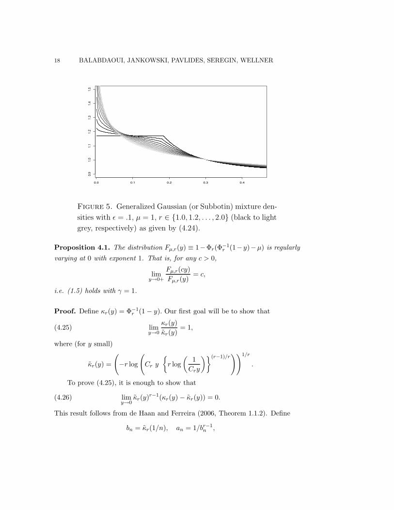
It is easily seen that g$,µ,r is monotone decreasing on (0, 1) and is unbounded atzero if r > 1. Figure 5 shows plots of these densities for $ = .1, µ = 1, and r *{1.0, 1.1, . . . , 2.0}. Note that g$,µ,1 is bounded at 0: in fact g$,µ,1(y) = 1# $+ $eµ

for 0 ( y ( 2"1e"µ.


0.0 0.1 0.2 0.3 0.4

0.91.0

1.11.2

1.31.4

1.5

Figure 5. Generalized Gaussian (or Subbotin) mixture den-

sities with # = .1, µ = 1, r * {1.0, 1.2, . . . , 2.0} (black to light

grey, respectively) as given by (4.24).

Proposition 4.1. The distribution Fµ,r(y) " 1#"r(""1r (1#y)#µ) is regularly

varying at 0 with exponent 1. That is, for any c > 0,

limy&0+

Fµ,r(cy)Fµ,r(y)

= c,

i.e. (1.5) holds with ! = 1.

Proof. Define &r(y) = ""1r (1 # y). Our first goal will be to show that

limy&0

&r(y)&r(y)

= 1,(4.25)

where (for y small)

&r(y) =

6#r log

6Cr y

*r log

(1

Cry

)+(r"1)/r771/r

.

To prove (4.25), it is enough to show that

limy&0

&r(y)r"1(&r(y) # &r(y)) = 0.(4.26)

This result follows from de Haan and Ferreira (2006, Theorem 1.1.2). Define

bn = &r(1/n), an = 1/br"1n ,


and choose F = "r in the statement of Theorem 1.1.2. Then, if we can showthat

n(1 # "r(anx + bn)) $ log G(x) " e"x, x * R,(4.27)

it follows from de Haan and Ferreira (2006, Theorem 1.1.2 and Section 1.1.2)that for all x * R

limy&0

U(x/y) # b)1/y*a)1/y*

= G"1(e"1/x) = log(1/x),

where U(t) = (1/(1 # "r))"1(t) = ""1r (1 # 1/t). Choosing x = 1 yields (4.26).

Therefore, we need to prove (4.27).To do this, we make use of the following, which is a generalization of Mills’

ratio to the generalized Gaussian family

1 # "r(z) & %r(z)zr"1

as z $ !.(4.28)

The statement follows from l’Hopital’s rule:

limz&'

" 'z %r(y)dy

z1"r%r(z)= lim

z&'

#%r(z)(1 # r)z"r%r(z) + z1"r%r(z)(#zr"1)

= limz&'

11 # (1 # r)z"r

= 1.

Now,

n(1 # "r(anx + bn)) & n%r(anx + bn)(anx + bn)r"1

=n

Crbr"1n

exp8# br

n

r

81 + anx

bn

9r9

(1 + anx/bn)r"1

& n

Crbr"1n

exp(#br

n

r

(1 +

rx

brn

))

= exp(#

(brn

r+ (r # 1) log bn # log n + log Cr

))exp(#x)

$ exp(#0) · exp(#x)

by using the definition of bn. We have thus shown that (4.25) holds.

Then, for y $ 0, by (4.28) and (4.25)

Fµ,r(y) = 1 # "r(&r(y) # µ) & 1 # "r(&r(y) # µ)

& %r(&r(y) # µ)(&r(y) # µ)r"1

.


Plugging in the definition of %r, we find that

Fµ,r(y) & 1/Cr

(&r(y) # µ)r"1exp

(# &r(y)r

r

''''1 # µ

&r(y)

''''r)

=1/Cr

(&r(y) # µ)r"1exp

*(log(Cry) + log(r log(1/(Cry))))

''''1 # µ

&r(y)

''''r)

=1/Cr

(&r(y) # µ)r"1(Cry)

˛˛1" µ

"r(y)

˛˛r

·*

r log1

Cry

+ r!1r

˛˛1" µ

"r(y)

˛˛r

.

Note that limy&0 &r(cy)/&r(y) = 1. Therefore,

Fµ,r(cy)Fµ,r(y)

& c

˛˛1" µ

"r(cy)

˛˛r

· (Cry)˛˛1" µ

"r(cy)

˛˛r"

˛˛1" µ

"r(y)

˛˛r

·(&r(y) # µ

&r(cy) # µ

)r"1

·

:r log 1

Crcy

; r!1r

˛˛1" µ

"r(cy)

˛˛r

:r log 1

Cry

; r!1r

˛˛1" µ

"r(y)

˛˛r

$ c · 1 · 1 · 1 = c.

Thus (1.5) holds with ! = 1. !

By the theory of regular variation (see e.g. Bingham et al. (1989, page 21)),this implies that Fµ,r(y) = y((y) where ( is slowly varying at 0. It then followseasily that (1.5) holds for F0 = G$,µ,r with exponent 1. Thus our theory ofSection 1 applies with an of Theorem 1.1 taken to be an = G$,µ,!(1/n); i.e.

1n

= G$,µ,r(an) = (1 # $)an + $Fµ,r(an) = $Fµ,r(an)

where the last approximation is valid for r > 1, but not for r = 1. When r = 1,the first equality can be solved explicitly, and we find:

an =

,1 # "r(""1

r (1 # (1/(n$))) + µ), when r > 1n"1(1 # $+ $eµ)"1, when r = 1.

(4.29)

We conclude that Theorem 1.1 holds for an as in the last display where !fn is theGrenander estimator of g$,µ,r based on Y1, . . . , Yn.

Another interesting mixture family to consider is as follows: suppose that"1, "2 are two fixed distribution functions: then

under H0 : F = "1,

under H1 : F = (1 # $)"1 + $"2, $ * (0, 1).


Using the transformation to Yi " 1 # "1(Xi) & G, then, for 0 ( y ( 1 we findthat under H1 the distribution of the Yi’s is given by

G(y) = (1 # $)y + $(1 # "2(""11 (1 # y))),

g(y) = (1 # $) + $%2(""1

1 (1 # y))%1(""1

1 (1 # y)).

For "2 given in terms of "1 by the (Lehmann alternative) distribution function"2(y) = 1 # (1 # "1(y))! , this becomes

G(y) = (1 # $)y + $y! ,

g(y) = (1 # $) + $!y!"1.

When 0 < ! < 1 this family fits into the framework of our condition G2 with# = 1 # ! and C2 = $!.

4.2. Estimation of the contaminating density. Suppose that G$,F (y) = (1#$)y + $F (y) where F is a concave distribution on [0, 1] with monotone decreasingdensity f . Thus the density g$,F of G$,F is given by g$,F (y) = (1#$)+$f(y). Notethat g$,F is also monotone decreasing, and g$,F (y) ) 1#$+$f(1) = 1#$ = g$,F (1)if f(1) = 0. For $ > 0 we can write

f(y) =g$,F (y) # (1 # $)

$.

If Y1, . . . , Yn are i.i.d. g$,F then we can estimate g$,F by the Grenander estimator!gn, and we can estimate $ by

!$n = 1 # !gn(1).

This results in the following estimator !fn of the contaminating density f :

!fn(y) =!gn(y) # (1 # !$n)

!$n=

!gn(y) # !gn(1)1 # !gn(1)

,

which is quite similar in spirit to a setting studied by Swanepoel (1999). Here,however, we propose using the shape constraint of monotonicity, and hence theGrenander estimator, to estimate both $ and f . We intend to study this estimatorelsewhere.


Appendix A: Proofs for Section 1

Before proving Theorem 1.1, we need the following two lemmas. The firstlemma shows that the functionals argmaxR and argmaxL are both Op(1), whilethe second shows these are equivalent almost surely for the limiting Poisson pro-cess. Together, these two lemmas will show that both functionals argmaxR andargmaxL are continuous. Below we assume that (1.5) holds and that nF0(an) & 1.Thus both (1.3) and (1.7) also hold.

Lemma 5.2. (i) When ! = 1 and x > 1, argmaxL,Rv {nFn(anv) # xv} = Op(1).

(ii) When ! * (0, 1) and x > 0, argmaxL,Rv {nFn(anv) # xv} = Op(1).

Proof. It su!ces to show that

lim supn&'

P (supv!K

{nFn(anv) # xv} ) 0) $ 0, as K $ !

under the conditions specified. Let h(x) = x(log x#1)+1 and recall the inequality

P (Bin(n, p)/(np) ) t) ( exp(#nph(t))

for t ) 1 where Bin(n, p) denotes a Binomial(n, p) random variable; see e.g.Shorack and Wellner (1986, inequality 10.3.2, page 415). It follows that

P (supv!K

{nFn(anv) # xv} ) 0)

= P (0'j=K{nFn(anv) # xv ) 0 for some v * [j, j + 1)})

('.

j=K

P (nFn(an(j + 1)) # xj ) 0)

='.

j=K

P

(nFn(an(j + 1))nF0(an(j + 1))

) xj

nF0(an(j + 1))

)

('.

j=K

exp(#nF0(an(j + 1))h

(xj

nF0(an(j + 1))

))(5.30)

Next, since F0 is concave,

nF0(an(j + 1)) ( nF0(an(K + 1))j + 1K + 1

for j ) K and nF0(an(K +1)) $ (K +1)! and n $ !. Therefore, for all j ) K

and su!ciently large n, we havexj

nF0(an(j + 1))) )(K + 1)1"! xj

j + 1


for any fixed ) < 1. We need to handle the two cases ! = 1 and ! < 1 separately.Note that if ! < 1, then the above display shows that K,n can be chosen su!-ciently large so that (xj)/nF0(an(j+1)) is uniformly large. On the other hand, if! = 1 and x > 1 then we can pick ),K, n large enough so that (xj)/nF0(an(j+1))is strictly greater than 1 + $ for some $ > 0, again uniformly in j.

Suppose first that ! < 1. Then for K,n large, since h(x) & x log x as x $ !,there exists a constant 0 < C < 1 such that for all j ) K

nF0(an(j + 1))h(

xj

nF0(an(j + 1))

)) C(xj) log

(xj

j + 1

)

) Cx(xj),

for some other constant Cx > 0. This shows that the sum in (5.30) converges tozero as K $ !, as required.

Suppose next that ! = 1. Note that the function h(x) > 0 for x > 1.Therefore, combining our arguments above, we find that for all j ) K

nF0(an(j + 1))h(

xj

nF0(an(j + 1))

)) )(j + 1)h

(xj

nF0(an(j + 1))

)

) Cx,%(j + 1),

again for some Cx,% > 0. This again implies that the sum in (5.30) converges tozero as K $ !, and completes the proof. !

Lemma 5.3. Suppose that ! * (0, 1]. Then

V Lx " argmaxL

v {N(v!) # xv} = argmaxRv {N(v!) # xv} " V R

x a.s.

Proof. Suppose that V Lx < V R

x . Then it follows that N((V Lx )!) # xV L

x =N((V R

x )!) # xV Rx , or, equivalently

N((V Rx )!) # N((V L

x )!) = x{V Rx # V L

x }.

Now (V Rx )! , (V L

x )! * J(N) " {t > 0 : N(t) # N(t#) ) 1}, so the left sideof the last display takes values in the set {1, 2, . . .}, while the right side takesvalues in x · {r1/! # s1/! : r, s * J(N), r > s}. But it is well-known that all the(joint) distributions of the points in J(N) are absolutely continuous with respectto Lebesgue measure, and hence the equality in the last display holds only forsets with probability 0. !


Proof of Theorem 1.1: We first prove convergence of the one-dimensionaldistributions of nan

!fn(ant). Fix K > 0, and let x > 1{!=1} and t * (0,K]. Bythe switching relation (2.12),

P (nan!fn(ant) ( x) = P (!sL

n(x/(nan)) ( ant)

= P (argmaxLs {Fn(s) # xs/(nan)} ( ant)

= P (argmaxLv {Fn(van) # x(v/n)} ( t)

= P (argmaxLv {nFn(van) # xv} ( t)

$ P (argmaxLv {N(v!) # xv} ( t)

= P (!h!(t) ( x)

where the convergence follows from (1.7), and the argmax continuous mappingtheorem for D[0,!) applied to the processes {v ,$ nFn(van) # xv : v ) 0}; seee.g. Ferger (2004, Theorem 3 and Corollary 1). Note that Lemma 5.2 yields theOp(1) hypothesis of Ferger’s Corollary 1, while Lemma 5.3 shows that equalityholds in the limit conclusion.

Convergence of the finite-dimensional distributions of !hn(t) " nan!fn(ant)

follows in the same way by using the process convergence in (1.7) for finitelymany values (t1, x1), . . . , (tm, xm) where each tj * R+ and xj > 1{!=1}.

To verify tightness of !hn in D[0,!) we use Billingsley (1999, Theorem 16.8).Thus, it is su!cient to show that for any K > 0, and any $ > 0

limM&'

lim supn

P

6

sup0%t%K

|!hn(t)| ) M

7

= 0(5.31)

lim%&0

lim supn

P8w%,K(!hn) ) $

9= 0,(5.32)

where w%,K(h) is the modulus of continuity in the Skorohod topology defined as

w%,K(h) = inf{ti}r

max0<i%r

sup {|h(t) # h(s)| : s, t * [ti"1, ti) 1 [0,K]} ,

where {ti}r is a partition of [0,K] such that 0 = t0 < t1 < . . . < tr = K

and ti # ti"1 > ). Suppose then that h is a piecewise constant function withdiscontinuities occurring at the (ordered) points {*i}i!0. Then if ) ( infi |*i #*i"1| we necessarily have that w%,K(h) = 0.


First, note that since !hn is non-increasing,

%!hn%m0 " sup

0%t%m|!hn(t)| = !hn(0),

and hence (5.31) follows from the finite-dimensional convergence proved above.Next, fix $ > 0. Let 0 = *n,0 < *n,1 < · · · < *n,Kn < K denote the (ordered)

jump points of !hn, and let 0 = Tn,0 < Tn,1 < · · · < Tn,Jn < K denote the (again,ordered) jump points of nFn(ant). Because {*n,1, . . . , *n,Kn} -{ Tn,1, . . . , Tn,Jn},it follows that inf{*i,n # *i"1,n} ) inf{Ti,n # Ti"1,n} and hence

P8w%,K(!hn) ) $

9( P

(inf

i=1,...,Jn

{Ti,n # Ti"1,n} < )

).

Now, by (1.7) and continuity of the inverse map (see e.g. Whitt (2002, Theorem13.6.3, page 446))

(Tn,1, . . . , Tn,Jn, 0, 0, . . .) + (T 1/!1 , . . . , T 1/!

J , 0, 0, . . .),

where T1, . . . , TJ denote the successive arrival times on [0,K] of a standard Pois-son process. Thus,

lim%&0

P

(inf

i=1,...,J{T 1/!

i # T 1/!i"1} < )

)= 0.

and therefore (5.32) holds. This completes the proof of (i).Now we prove (ii): Fix 0 < c < !. We first write

sup0<x%can

'''''!fn(x)f0(x)

# 1

''''' = sup0<t%c

'''''nan

!fn(tan)nanf0(tan)

# 1

''''' .(5.33)

Suppose we could show that the ratio process nan!fn(ant)/nanf0(ant) converges

to the process t1"!!h!(t)/! in D[0,!). Then the conclusion follows by notingthat the functional h ,$ sup0<t%c |h| is continuous in the Skorohod topologyas long as c is not a point of discontinuity of h (Jacod and Shiryaev (2003,Proposition VI 2.4, page 339)). Since N(t!) is stochastically continuous (i.e.P (N(t!) # N(t!#) > 0) = 0 for each fixed t > 0), t1"!!h!(t)/! is almost surelycontinuous at c.

It remains to prove convergence of the ratio. Fix K > c, and again we mayassume that K is a continuity point. Consider first the term in the denominator,nanf0(ant): it follows from (1.4) that

gn(t) " (nanf0(ant))"1 $ !"1t1"! " g(t)


where g is monotone increasing and uniformly continuous on [0,K]. Thus gn $ g

in C[0,K]. Since the term in the numerator satisfies hn(t) " nan!fn(ant) +

!h!(t) " h(t) in D[0,K], it follows that gnhn + gh in D[0,K], as required. Here,we have again used the continuity of the supremum. This completes the proofof (ii). !

Before proving Corollaries 1.2 - 1.4 we state the following lemma.

Lemma 5.4. Suppose that an = p(1/n) for some function with p(0) = 0 satisfy-ing limx&0+ p$(x)f0(p(x)) = 1. Then nF0(an) $ 1.

Proof: This follows easily from l’Hopital’s rule, since

limn&'

nF0(an) = limx&0+

F0(p(x))x

= limx&0+

f0(p(x))p$(x).

!Proof of Corollary 1.2: Under the assumption G0 we see that F0(x) &f0(0+)x as x $ 0, so (1.5) holds with ! = 1. The claim that an = 1/(nf0(0+))satisfies nF0(an) $ 1 follows from Lemma 5.4 with p(x) = x/f0(0+). For (i) notethat !h1(0) = !h1(0+) = supt>0(N(t)/t), and the indicated equality in distributionfollows from Pyke (1959); see Proposition 1.5 and its proof. (ii) follows directlyfrom (i) of Theorem 1.1. To prove (iii), note that from (ii) of Theorem 1.1 itsu!ces to show that

sup0<t%c

'''!h1(t) # 1''' =

'''!h1(0+) # 1''' = !h1(0+) # 1 = Y1 # 1(5.34)

for each c > 0 where !h1(t) is the right derivative of the LCM of N(t). The equalityin (5.34) holds if !h1(c) > 1, since !h1 is decreasing by definition. By the switchingrelation (2.12), we have the equivalence

{!h1(c) > 1} = {!sL(1) > c}.

The equality in (5.34) thus follows if !sL(1) = !. That is, if

N(t) # t < supy!0

{N(y) # y} for all finite t.

Let W = supy!0{N(y) # y}. Pyke (1959, pages 570-571) showed that P (W (x) = 0 for x ) 0; i.e. P (W = !) = 1. !

Proof of Corollary 1.3: Under the assumption G1 we see that F0(x) &C1x(log(1/x))" as x $ 0, so (1.5) holds with ! = 1. The claim that an =


1/(C1n(log n)") satisfies nF0(an) $ 1 follows from Lemma 5.4 with p(x) =x/(C1 log(1/x))" . For (i) note that !h1(0) = !h1(0+) = supt>0(N(t)/t) just as inthe proof of Corollary 1.2. (ii) again follows directly from (i) of Theorem 1.1,and the proof of (iii) is just the same as in the proof of Corollary 1.2. !

Proof of Corollary 1.4: Under the assumption G2 we see that F0(x) &C2x1"#/(1 # #) as x $ 0, so (1.5) holds with ! = 1 # #. The claim thatan = {(1##)/(nC2)}1/(1"#) satisfies nF0(an) $ 1 follows from Lemma 5.4 withp(x) = ((1 # #)x/C2)1/(1"#). For (i) note that

!h1"#(0) = !h1"#(0+) = supt>0

(N(t1"#)/t) = sups>0

(N(s)/s1/(1"#))

much as in the proof of Corollary 1.2. (ii) and (iii) follow directly from (i) and(ii) of Theorem 1.1. !

Proof of Proposition 1.5: The part of the proposition with ! = 1 follows fromPyke (1959, pages 570-571); this is closely related to a classical result of Daniels(1945) for the empirical distribution function; see e.g. Shorack and Wellner (1986,Theorem 9.1.2, page 345).

The proof for the case ! < 1 proceeds much along the lines of Mason (1983,pages 103–105). Fix x > 0 and ! < 1. We aim at establishing an expression forthe distribution function of Y! " sups>0(N(s)/s1/!) at x > 0. First, observe that

P (Y! ( x) = P

(sups>0

*N(s)s1/!

+( x

)

= P (N(t) ( U(t) for all t > 0)(5.35)

where the function U(t) = xt1/! . For j * N let tj := (j/x)! , and note thatt1 < t2 < . . . and U(tj) = j.

Define sets B and C by

B " [N(tk) /= k ; for all k ) 1] and C " [N(s) > U(s) ; for some s > 0].

Then P (B 1 C) = 0 as a consequence of the following argument: Suppose thatthere exists some t > 0 and k * N such that k = N(t) > U(t) and N(ti) /= i, for alli ) 1. It then follows that tk > t, for otherwise it follows that k = U(tk) ( U(t),as U(·) is increasing, which is a contradiction. Therefore, tk > t implies thatN(tk) > N(t) = k, as N(·) is non–decreasing while N(tk) = k is disallowed,by hypothesis. Hence, N(ti) > i holds true for all i ) k, for otherwise there


would exist some j ) k such that N(tj) = j, since N(·) is a counting process.Therefore, for each i ) k we have that N(s) ) i + 1 holds for all ti ( s ( ti+1

and, consequently, that N(s) ) U(s) holds for all s ) tk. This implies thatB 1 C . [lim infs&'{N(s)/s1/!} ) x] and therefore P (B 1 C) = 0, since theSLLN implies that N(s)/s1/! $ 0 holds almost surely, for fixed ! < 1. We thusconclude that P (B 1 C) = 0.

We conclude that P (C) = P (C 1 Bc). Furthermore, since U is a strictlyincreasing function, and since N has jumps at the points {tk} with probabilityzero, we also find that P (C 1 Bc) = P (Bc). Finally, partition Bc as Bc =0'

k=1Ak for the disjoint sets Ak " [N(tk) = k, N(tj) /= j for all 1 ( j < k], k ) 1.Combining all arguments above, we conclude that

P (Y! ( x) = 1 # P (C) = 1 #'.

k=1

P (Ak)

where P (A1) = P (N(t1) = 1) = p(t1; 1), and, for k ) 2, P (Ak) may be writtenas

P (N(tk) = k) # P ({N(tk) = k} 1 {N(ti) /= i, i < k}c)

= P (N(tk) = k) #k"1.

j=1

P (N(tk) = k, N(tj) = j, N(ti) /= i, i < j)

= P (N(tk) = k) #k"1.

j=1

P (N(tk) # N(tj) = k # j)P (N(tj) = j, N(ti) /= i, i < j).

The result follows. !

Appendix B: Definitions from Convex Analysis

The epigraph (hypograph) of a function f from a subset S of Rd to [#!,+!]is the subset epi(f) (hypo(f)) of Rd+1 defined by

epi(f) = {(x, t) : x * S, t * R, t ) f(x)},

hypo(f) = {(x, t) : x * S, t * R; t ( f(x)}.

The function f is convex if epi(f) is a convex set. The e!ective domain of aconvex function f on S is

dom(f) = {x * Rd : (x, t) * epi(f) for some t} = {x * Rd : f(x) < !}.


The t#sublevel set of a convex function f is the set Ct = {x * dom(f) :f(x) ( t}, and the t#superlevel set of a concave function g is the set St = {x *dom(g) : g(x) ) t}. The sets Ct, St are convex. The convex hull of a set S - Rd,denoted by conv(S), is the intersection of all the convex sets containing S.

A convex function f is said to be proper if its epigraph is non-empty andcontains no vertical lines; i.e. if f(x) < +! for at least one x and f(x) > #!for every x. Similarly, a concave function g is proper if the convex function #g isproper. The closure of a concave function g, denoted by cl(g), is the pointwiseinfimum of all a!ne functions h ) g. If g is proper, then

cl(g)(x) = lim supy&x

g(y).

For every proper convex function f there exists closed proper convex functioncl(f) such that epi(cl(f)) " cl(epi(f)). The conjugate function g+ of a concavefunction g is defined by

g+(y) = inf{2x, y3 # g(x) : x * Rd},

and the conjugate function f+ of a convex function f is defined by

f+(y) = sup{2x, y3 # f(x) : x * Rd}.

If g is concave, then f = #g is convex and f has conjugate f+(y) = #g+(#y).A complete non-decreasing curve is a subset of R2 of the form

$ = {(x, y) : x * R, y * R, +"(x) ( y ( ++(x)}

for some non-decreasing function + from R to [#!,+!] which is not everywhereinfinite. Here ++ and +" denote the right and left continuous versions of +respectively. A vector y * Rd is said to be a subgradient of a convex function f

at a point x if

f(z) ) f(x) + 2y, z # z3 for all z * Rd.

The set of all subgradients of f at x is called the subdi!erential of f at x, andis denoted by 'f(x).

A face of a convex set C is a convex subset B of C such that every closedline segment in C with a relative interior point in B has both endpoints in B.If B is the set of points where a linear function h achieves its maximum over C,then B is a face of C. If the maximum is achieved on the relative interior of a


line segment L - C, then h must be constant on L and L - B. A face B of thistype is called an exposed face.

References

Anevski, D. and Soulier, P. (2009). Monotone spectral density estimation. Tech.rep., University of Lund, Department of Mathematics.

Beran, J. (1994). Statistics for long-memory processes, vol. 61 of Monographs onStatistics and Applied Probability. Chapman and Hall, New York.

Billingsley, P. (1999). Convergence of Probability Measures. 2nd ed. John Wiley& Sons Inc., New York.

Bingham, N. H., Goldie, C. M. and Teugels, J. L. (1989). Regular Variation,vol. 27 of Encyclopedia of Mathematics and its Applications. Cambridge Uni-versity Press, Cambridge.

Boyd, S. and Vandenberghe, L. (2004). Convex Optimization. Cambridge Uni-versity Press, Cambridge.

Cox, D. R. (1984). Long-range dependence: A review. In Statistics: An Appraisal(H. A. David and H. T. David, eds.). Iowa State University.

Daniels, H. E. (1945). The statistical theory of the strength of bundles of threads.I. Proc. Roy. Soc. London. Ser. A. 183 405–435.

de Haan, L. and Ferreira, A. (2006). Extreme Value Theory. Springer Series inOperations Research and Financial Engineering, Springer, New York.

Devroye, L. (1986). Nonuniform Random Variate Generation. Springer-Verlag,New York.

Devroye, L. (1987). A Course in Density Estimation, vol. 14 of Progress inProbability and Statistics. Birkhauser Boston Inc., Boston, MA.

Donoho, D. and Jin, J. (2004). Higher criticism for detecting sparse heterogeneousmixtures. Ann. Statist. 32 962–994.

Ferger, D. (2004). A continuous mapping theorem for the argmax-functional inthe non-unique case. Statist. Neerlandica 58 83–96.

Gnedenko, B. (1943). Sur la distribution limite du terme maximum d’une seriealeatoire. Ann. of Math. (2) 44 423–453.

Gneiting, T. (2000). Power-law correlations, related models for long-range de-pendence and their simulation. J. Appl. Probab. 37 1104–1109.


Grenander, U. (1956a). On the theory of mortality measurement. I. Skand.Aktuarietidskr. 39 70–96.

Grenander, U. (1956b). On the theory of mortality measurement. II. Skand.Aktuarietidskr. 39 125–153 (1957).

Groeneboom, P. (1985). Estimating a monotone density. In Proceedings of theBerkeley conference in honor of Jerzy Neyman and Jack Kiefer, Vol. II (Berke-ley, Calif., 1983). Wadsworth Statist./Probab. Ser., Wadsworth, Belmont, CA.

Jacod, J. and Shiryaev, A. N. (2003). Limit Theorems for Stochastic Processes,vol. 288 of Grundlehren der Mathematischen Wissenschaften [FundamentalPrinciples of Mathematical Sciences]. 2nd ed. Springer-Verlag, Berlin.

Kulikov, V. N. and Lopuhaa, H. P. (2005). Asymptotic normality of the Lk-errorof the Grenander estimator. Ann. Statist. 33 2228–2255.

Kulikov, V. N. and Lopuhaa, H. P. (2006). The behavior of the NPMLE ofa decreasing density near the boundaries of the support. Ann. Statist. 34742–768.

Ma, C. (2002). Correlation models with long-range dependence. J. Appl. Probab.39 370–382.

Martin, R. J. and Walker, A. M. (1997). A power-law model and other modelsfor long-range dependence. J. Appl. Probab. 34 657–670.

Mason, D. M. (1983). The asymptotic distribution of weighted empirical distri-bution functions. Stochastic Process. Appl. 15 99–109.

Miller, D. R. (1976). Order statistics, Poisson processes and repairable systems.J. Appl. Probability 13 519–529.

Pyke, R. (1959). The supremum and infimum of the Poisson process. Ann. Math.Statist. 30 568–576.

Rockafellar, R. T. (1970). Convex Analysis. Princeton Mathematical Series, No.28, Princeton University Press, Princeton, N.J.

Rockafellar, R. T. and Wets, R. J.-B. (1998). Variational Analysis, vol. 317 ofGrundlehren der Mathematischen Wissenschaften [Fundamental Principles ofMathematical Sciences]. Springer-Verlag, Berlin.

Shorack, G. R. and Wellner, J. A. (1986). Empirical Processes with Applica-tions to Statistics. Wiley Series in Probability and Mathematical Statistics:Probability and Mathematical Statistics, John Wiley & Sons Inc., New York.


Swanepoel, J. W. H. (1999). The limiting behavior of a modified maximal sym-metric 2s-spacing with applications. Ann. Statist. 27 24–35.

van de Geer, S. (1993). Hellinger-consistency of certain nonparametric maximumlikelihood estimators. Ann. Statist. 21 14–44.

van der Vaart, A. and van der Laan, M. J. (2006). Estimating a survival distribu-tion with current status data and high-dimensional covariates. Int. J. Biostat.2 Art. 9, 42.

van der Vaart, A. W. and Wellner, J. A. (1996). Weak Convergence and EmpiricalProcesses. Springer Series in Statistics, Springer-Verlag, New York.

Whitt, W. (2002). Stochastic Process Limits. Springer Series in OperationsResearch, Springer-Verlag, New York.

Woodroofe, M. and Sun, J. (1993). A penalized maximum likelihood estimate off(0+) when f is nonincreasing. Statist. Sinica 3 501–515.

Centre de Recherche en Mathematiques de la DecisionUniversite Paris-Dauphine, Paris, France

E-mail: [email protected]

Department of Mathematics and StatisticsYork University, Toronto, Canada


Department of Mechanical EngineeringFrederick University Cyprus, Nicosia, Cyprus


Department of StatisticsUniversity of Washington, Seattle, USA


Department of StatisticsUniversity of Washington, Seattle, USA


On the Grenander estimator at zero

Documents

Transcript of On the Grenander estimator at zero