TriTone: a radiofrequency field ( B 1)-insensitive T 1 estimator for MRI at high magnetic fields

TRITONE: a Radio-Frequency Field (B1) Insensitive T1 Estimatorfor MRI at High Magnetic Fields.★

Roman Fleyshera, Lazar Fleyshera, Songtao Liua, and Oded Gonena,*aDepartment of Radiology, NYU School of Medicine 650 First Ave, 6th floor New York, NY 10016USA

AbstractFast, high resolution, longitudinal relaxation time (T1) mapping is invaluable in clinical and researchapplications. It has been shown that two spoiled gradient recalled echo (SPGR) images acquired insteady state with variable flip angles is an attractive alternative to the multi-image sets previouslyacquired with inversion or saturation recovery. The known sensitivity of the two-point method totransmit radio-frequency field (B1) inhomogeneity exacerbated at 3 Tesla and above, however,mandates its combination with an additional, time consuming and possibly SAR intensive B1measurement, preventing direct migration of the method to these fields. To address this we introducea method designed to be free of systematic errors caused by B1 inhomogeneity in which the value ofT1 is extracted from three SPGR images acquired with EPI readout. The precision of the T1 mapsproduced is found to be comparable to the two-point method while the accuracy is greatly improvedin the same time and spatial resolution. A welcome byproduct of the method is a map of B1 that canbe used to correct other acquisitions in the same session. Tables of the optimal acquisition protocolsare provided for several total imaging times.

KeywordsT1 mapping; fast volumetric imaging; high-field MRI; quantitative MRI; RF inhomogeneity;optimization methods

IntroductionThe current most efficient strategy for obtaining T1 maps within clinically acceptable time isbased on acquiring two spoiled gradient recalled echo (SPGR) images in steady states withvariable flip angles [1,2]. Although the method's efficiency can be maximized by introducingvarious repetition times and number of averages used to acquires each image in the pair [3],its fundamental premise remains: The actual values of the flip angles experienced by the spinsare necessary for accurate T1 calculation. Fortunately, at 1.5 Tesla the imprecise knowledgeof these angles caused by a combination of radio-frequency (RF) pulse imperfections, transmitcoil profiles, standing wave effects, etc. results only in insignificant bias in T1 [4]. At higherfield strengths, however, the transmit RF inhomogeneity (B1) becomes progressively worse.It leads to systematic errors in T1 that can no longer be neglected, preventing direct migrationof the two-point method to 3 T and above. For example, Cheng et. al. [5] considered the two-SPGR technique and showed that a ±15% deviation in flip angle, a level of non-uniformityoften encountered in vivo and in vitro at 3 T [5-7], will cause a ±30% systematic error in T1.

★This work is supported by NIH grants number EB001015, CA111911 and NS050520.*Corresponding author. Email address: [email protected] (Oded Gonen)..

NIH Public AccessAuthor ManuscriptMagn Reson Imaging. Author manuscript; available in PMC 2009 September 3.

Published in final edited form as:Magn Reson Imaging. 2008 July ; 26(6): 781–789. doi:10.1016/j.mri.2008.01.024.

NIH

-PA Author Manuscript

NIH


NIH


This undermines the entire reason of T1 determination, be it tissue segmentation, pathologyidentification or measurement of contrast agent uptake.

In order to take advantage of the increased sensitivity offered by high field scanners adiabaticpulses that deliver uniform excitation [8] can be employed. Specific absorption rate (SAR)limits, however, especially at high fields, may lower the efficiency or even preclude thisapproach. In general, given a particular hardware setup, the only way to cope with the SARlimit is to decrease or re-design the flip angles and/or increase the time intervals between them,rendering the SAR a sequence design restriction. An alternative approach to mitigate the B1inhomogeneity is to map it in situ using a separate B1 measuring sequence [5,7]. Unfortunately,it is time consuming and possibly SAR prohibitive in itself. In addition, B1 measurementuncertainty propagates into the error of T1 estimate, further reducing the overall efficiency ofthe scheme. Other solutions offered in the literature employ different sequences, requiringvarious RF power levels, imaging time and post processing needs [5,7,9-13]. Ultimately,regardless of the approach, the quality of T1 estimation is given by its measurement errorσT1 achieved in a given experimental time which includes the duration of calibration scans (ifany) [3,5,7,10,14].

In the present paper, we introduce a new method based on three SPGR echo sequences forT1 quantification that is insensitive to flip angle inhomogeneities and examine the sequenceparameters that influence the precision of its T1 estimation. Owing to the SPGR-triplet-for-T1-estimation approach, we name this new method TRITONE. We show that despite thecomplication caused by flip angle non-uniformity, TRITONE attains precision of T1 estimationcomparable to that achieved by the two-SPGR methods [1-3] in the same time and spatialresolution and exceeds them in accuracy. If the two-SPGR methods are combined with B1measurement for accuracy, then TRITONE supersedes them in precision. The post processingstep of TRITONE is straightforward and can be incorporated into on-line reconstruction.

TheorySince we wish to develop a method for T1 estimation to be used in clinical settings, we considerfield of view (FOV), spatial resolution and total allocated examination time (T) as exogenousvariables determined by the experimenter. The remaining SPGR sequence parameters: nominalflip angle (α), repetition time (TR), number of averages of a scan (N), echo time (TE) andreadout duration (Tadc) are to be optimized for the highest quality in the resultant T1 mapsregardless of the unknown spatial flip angle non-uniformity. The observed SPGR intensity(S) in each pixel is a function of the sequence parameters, longitudinal (T1) and transverse( ) relaxation times, flip angle inhomogeneity described by the actual-to-nominal flip angleratio (B1) and a factor proportional to the equilibrium magnetization (ρ0):

(1)

From the structure of this equation it is clear that having three images Sm, m = 1, 2, 3, acquiredwith di erent TR's and/or flip angles is su cient to estimate T1. Indeed, if the three share identicalbandwidth, readout, FOV and spatial resolution (to ensure identical reconstruction artifactsand weighting), then the ratio of any two images depends only on the unknown T1 and B1in a pixel. Therefore, a pair of such ratios, say S1/S3 and S2/S3, or equivalently a pair of spherical

angles ϕ = arctan(S3, S1) and are related to T1 and B1. Given sequenceparameters, a two dimensional look-up table T1(ϕ, θ) can be easily generated and then polledfor fast, on-line, T1 extraction. The precision of the result depends on the SNR of the raw

Fleysher et al.

Magn Reson Imaging. Author manuscript; available in PMC 2009 September 3.

NIH


NIH


NIH


images, sequence settings (TRm, αm, Nm, TE, Tadc) and on the actual values of T1 and B1 in thatpixel.

The sequence parameter optimization will be performed with the goal of minimizing thestandard deviation, σT1, of T1 estimation in the vicinity of the “expected” relaxation time

. Since ±15% variations in B1 around the “expected” are common at 3 Tesla[5-7] we will minimize the “average error” at and :

(2)

The choice of TE and Tadc (Tadc ≤ 2TE) does not alter the spin excitation memory underinvestigation but a ects SNR and with it — the T1 estimation precision. Their influence wasconsidered in [3] where it was shown that the SNR due to decay is proportional to

(eq. (2) of [3]). Knowing that this function attains its maximum at , weconsider SNR at this readout as a benchmark that is SNR at any other Tadc will be a fractionof the maximum given by:

(3)

Since the SNR of the raw images also depends on the RF coil, receiver hardware, spatialresolution, spin density and its T1, it is convenient to introduce a benchmark that wouldsummarize all these properties and enable hardware and sample independent comparison ofdifferent sequences and protocols. One such measure that lends itself to the task is the maximumSNR attainable by running the SPGR sequence at the Ernst angle with the optimal readout inthe same total imaging time as the proposed TRITONE experiment. Under these conditions

the image intensity (Eq. 1) is given by , so that the SNR

achieved by averaging SPGR images over time T is given by (see Eq.4.3.26 in [15]) which increases monotonically as TR diminishes and approaches the maximumvalue of

(4)

where σ0 is the standard deviation of the noise in a single image before averaging.

Using these results, χ2 fitting [16] is executed to relate the standard deviation of T1 to the threeSPGR sequence parameters (see appendix A for full derivation):

(5)

Fleysher et al.


NIH


NIH


NIH


where qm's are defined in Eq. (A.3) in the appendix and SNRmax is the maximal SNR (Eq. 4)

achievable in the time allocated: .

Similar to the two-SPGR T1 experiment [3], the error comprises three factors: (i) describinghardware and sample properties, (ii) accounting for signal decay and noise due to imagingreadout and (iii) reflecting sensitivity of the sequence to T1. It is thus the last two terms thatare subject to optimization and, in fact, of interest. Following [3], we will use a dimensionlessnormalized coefficient of variation, εT1, as a sample- and hardware-independent measure ofthe precision of T1 estimation:

(6)

where smaller εT1 indicates more efficient use of the imaging time for T1 estimation in additionto the usual “square root of time” law contained in SNRmax (Eq. 4). The normalized coefficientof variation corresponding to the average error to be minimized is then given by:

(7)

Observing the structure of Eqs. (5), (6) and (7), the derivation of the expression for entails

only redefinition of q's to , where qB1's are the same q's defined by Eq.(A.3) but evaluated at the corresponding B1's.

Minimization of this metric yields optimal acquisition parameters for T1 measurement in thevicinity of the assumed values of and . Nevertheless, once a protocol is chosen Eqs.(5) and (6) can be used to evaluate εT1 for any combinations of T1 and B1. The map of εT1(T1,B1) can then be examined on how the precision degrades as T1 and B1 deviate from their tuningvalues. The wider the region over which the error remains small, i.e. the flatter the map, thebetter. Choosing to minimize the average error at ±15% rather than that simply at helpsthis cause.

Materials and MethodsMinimization of the average normalized coefficient of variation was performed numericallyusing brute-force algorithm on a grid in the sequence-parameter space reported in Table 1. Thevalue of needed for numerical minimization (since it enters Eq. (5)), was chosen to be

as a good and practical approximation. It is however clear that if is substantiallydifferent, the minimization has to be repeated. The computation took several hours on a PentiumIV class workstation and yielded the set of acquisition parameters presented in Table 2. Thegranularity of the search grid is dictated by the numerical complexity of the problem. It istherefore possible that the absolute minimum was not reached. It is also possible that there areseveral minima. However, we are not interested in finding absolutely the best protocol perse, we only look for a protocol whose precision is as close to the absolute minimum as we canpractically get.

The experiments were done in a 3 T Trio whole body imager (Siemens AG, Erlangen, Germany)using its transmit-receive head coil, on a uniform 15cm diameter × 40cm length cylindrical

Fleysher et al.


NIH


NIH


NIH


water phantom and then in the brain of a volunteer. The volunteer was briefed on the procedureand gave institutional review board-approved written consent. Conventional 3D EPI data wasacquired with 192 × 192 × 96mm3 field of view and 64 × 64 × 32 matrix on a phantom andwith 224 × 224 × 64mm3 field of view and 224 × 224 × 64 matrix on a human head. As anexample, we chose a protocol from Table 2 (underlined) and acquired data assuming

in the phantom and in vivo. In order to satisfy the shortest TR, asindicated in Table 2, 32 k-space lines were acquired after each excitation in the phantomexperiment and 64 on the volunteer. The corresponding TEs were 13 and 45ms. After on-lineimage reconstruction, the three image values in each pixel were converted into the sphericalangles that were used to look up the values of T1 and B1 from the precomputed tables. Thelook-up table approach replaces computationally expensive non-linear χ2 fitting but isequivalent to it since the number of unknowns is equal to the number of images. Additionaladvantage of the approach is that the table can be generated during data acquisition while datais still unavailable dramatically reducing the postprocessing time.

The look-up table (Fig. 1) is a 300 × 3000 array in the (ϕ, θ) plane. Each of its cells of is filledwith the average value of T1 whose underlying spherical angles fall within it. Entries into thecells are generated by computing the corresponding SPGR intensity triplet using Eq. (1) andthen spherical angles for each combination of insteps of 0.001. The cells where the maximum and the minimum entries differ by more than

were marked as bad with a NAN (not-a-number). The table thus filled represents asingle valued function T1(ϕ, θ). In other words, for any measured intensity triplet, the sphericalangles are computed and then the corresponding T1 is unambiguously looked-up in the table(or NAN is assigned). The look up table B1(ϕ, θ) (not presented) was generated in a similarfashion.

After T1 and B1 in each pixel are determined, the – and receive-B1–weighted spin density,ρ0, is extracted from Eq. (1). Since the receive/transmit coil was used, following the reciprocityprinciple [17] the B1-corrected -weighted spin density is obtained by dividing the extractedvalue by the corresponding B1 in that pixel.

To illustrate the influence of the B1 inhomogeneity on T1 estimation we also acquired phantomdata using optimal two-point 3D EPI of the same total imaging time and tuning( ). The protocol was: TR1 = 30ms, α1 = 55°, N1 = 55, TR2 = 1440ms,α2 = 85°, N2 = 1 [3] with 32 k-space lines acquired after each excitation, as in TRITONE. Thisdata was processed as described in [3].

ResultsThe theoretically expected performance of the T1 estimation using selected protocol isdemonstrated in Fig. 2 where the map of normalized coefficient of variation, εT1, is presented.

Its minimal value is . (Note that Table 2 lists the average coefficient, , which islarger than the minimum.) The surface of this plot is flat for a wide range of T1's and B1's, thatis the precision remains within 20% of the minimum in the large, blue egg-shaped area( ).

Experimentally, a uniform phantom is the ideal test bed to evaluate the sensitivity of a methodto spatial B1 inhomogeneity. Since the phantom is uniform, its T1-map should be as well. AT1 map at a slice near the center of the excited volume is depicted in Fig. 3a. A histogram ofthe T1's, the width of which can be used to gauge the precision, is shown in Fig. 3b. If weassume that the width is due to noise alone (ignoring contributions due to possible remaining

Fleysher et al.


NIH


NIH


NIH


B1 inhomogeneity), the precision is rather remarkable, 1.8%. The B1 map in Fig. 3cdemonstrates a large flip angle non-uniformity that if left uncorrected would lead toconsiderable systematic errors in T1 estimation [5] (see below). Since a receive-transmit coilwas used, the reciprocity principle was utilized to correct for its receive profile and obtain a

-weighted spin density map (panel d). In analogy to the T1 map, the -weighted spin densityof the phantom should also be uniform. However, unlike the T1 map, is sensitive to theresidual B0 inhomogeneity that was not compensated by shimming, making it less uniform(Fig. 3d).

To appreciate the accuracy of the TRITONE method we present, in Fig. 4, a T1 map acquiredwith the nearest equivalent optimal 2-point method (with the same tuning and acquisition time).It is evident from the map (panel a) and the histogram (panel b) that uncorrected B1inhomogeneity is responsible for very large variation of T1's that is absent in Fig. 3b.

An in vivo 1×1×1 mm3 resolution map of T1 is shown in Fig. 5a. The histogram of the T1 values(panel b) exhibits a narrow peak at 950ms, a broad peak at about 1550ms and a tail at longerT1's. These features can be ascribed to the white matter, gray matter and CSF, respectively[13]. Although the in vivo B1 map (Fig. 5c) demonstrates less non-uniformity compared to thephantom, it is still substantial. Left uncorrected, it would result in large systematic errors inthe T1 map. The receive-coil-profile corrected -weighted spin density image is presented inFig. 5d. Note that the effects of residual B0 inhomogeneity that were not compensated byshimming are not apparent but can not be excluded.

DiscussionIn vivo and in vitro studies demonstrated that despite substantial efforts in coil design andexcitation pulse synthesis, the flip angles they produce still vary spatially at and above 3 T.This precludes the use of the current efficient two-SPGR method of T1 estimation [1,3] at thesefields, because it requires precise flip angles [5,7]. As a remedy we have proposed adding athird SPGR acquisition and showed how the unknown B1 inhomogeneity can be excluded inpost processing. We then presented a method for selecting the three sequence parameters toachieve the most efficient use of the available imaging time for T1 mapping. We havedemonstrated that the proposed TRITONE method of T1 estimation is indeed insensitive tospatial variations and deviations of B1 from its nominal value. All that remains is to comparethe performances of TRITONE with the two-SPGR methods.

Since time is at a premium in in vivo MRI, performance comparisons of different methods haveto be conducted assuming fixed total experiment duration including any time needed for thein situ B1 calibration scan. The normalized coe cient of variation εT1 at of the DESPOT1method [1] can be as small as 4.5 [3] which, even without accounting for the calibration scan'sduration, is worse than can be achieved with TRITONE (see Table 2). Combining the mostefficient two-point method [3], characterized by εT1 = 3.6, with a calibration scan (which canclaim more than 40% of the total time [5,7]) rises its normalized coefficient of variation abovethat of TRITONE at intermediate and long experiment durations ( ). Furthermore,B1 measurement error from the calibration scan has to be incorporated into the error of the finalT1 estimate making exact comparisons of the efficiencies more difficult and dependent on thecalibration procedure. Nevertheless, this contribution is not negligible because it is double theB1 measurement error [5]: ±15% deviation in B1 causes ±30% error in T1 and thus even if the2-point T1 measurement were noise-free, the error in T1 due to noise in the calibration scanalone would have been:

Fleysher et al.


NIH


NIH


NIH


(8)

Combining both sources of noise in quadrature (because noise in T1 and B1 measurements areindependent) we can write for the precision of B1-corrected 2-point method:

(9)

where we assumed 60%/40% split of the total experimental time for T1 and B1 measurements,

as above. The normalized coefficient of variation for calibration scan, , depends on theprotocol. For the sake of the argument let's assume that calibration is very precise, so that

. Then, making TRITONE the most

efficient at about (see in Table 2).

The two-point approach remains the method of choice for dynamic T1 studies where acquisitiontime available must be short. In these studies the B1 map acquired with a calibration scan maybe assumed to be time invariant. To maintain high accuracy of B1-corrected T1's the excitationpulse and slice selection should be identical in the calibration and T1 mapping sequences, afeature automatically offered by the TRITONE method.

Similar to previous studies [1-3,5,7,10], we assumed a single compartment model, i.e., that thesignal from each pixel is characterized by unique values of T1 and B1. While this assumptioncan definitely be satisfied for T1 in phantoms, uniqueness of B1 is always an approximation.Unaccounted intravoxel flip angle variation, especially at the edges of the excited volume andintravoxel T1 variation produce systematic errors in T1 estimation. They may even lead toseemingly impossible signal behavior that can not be described by Eq. (1). In the previous andthe presented methods such a situation can also arise due to sample motion throughmisregistration between images or disruption of the steady state. For the above reasons, 3Dexcitations (used here) which have more uniform excitation profiles than 2D ones are preferred.

In the numerical optimization leading to Table 2 all parameters were allowed to vary withoutany restrictions (within the search grid of Table 1). At higher fields, however, it may benecessary to exclude certain TR and flip angle combinations in order to satisfy SAR restrictionswhich are pulse shape and transmit coil dependent and thus need to be evaluated on a case bycase basis. However, a protocol that passes SAR limits at high fields is likely to do so at lowfields as well. Therefore, common protocol with identical look-up table can be utilized acrossall such fields.

Finally, we note that while we utilized the commercially available 3D EPI SPGR sequence, itwould be simple to setup spiral, radial or any other type of SPGR sequence under the TRITONEumbrella to generate B1-invariant T1 maps. This is because the choice of k-space trajectorydoes not interfere with the spin excitation history and the only user-selectable parameters arethe FOV, spatial resolution, and total examination time. The remaining SPGR sequenceparameters are derived from these inputs through Table 2.

Fleysher et al.


NIH


NIH


NIH


ConclusionFast efficient high resolution T1 mapping techniques rely on precise knowledge of flip anglesfor accurate determination of the relaxation rate. Unfortunately, at higher magnetic fields thenotion of flip angle is poorly defined due to non-uniform transmit coil profiles, wave effects,etc., degrading the accuracy of many quantitative techniques. The proposed TRITONE methodaddresses the issue of B1 inhomogeneity by collecting three conventional 3D SPGR EPI imagesto produce both unbiased and precise T1 maps. The post processing step, althoughcomputationally somewhat more involved than in the two-point methods, is stillstraightforward and can be incorporated into on-line reconstruction.

Appendix

Appendix AIn the χ2 fitting procedure, the variances of the estimated parameters are related to the variances

of the average images Sm through the diagonal elements of the covariance matrix C = (AT

A)−1 where m-th row of matrix A is given by [16]

(A.1)

Since in the problem considered the number of unknowns is equal to the number of images,the matrix A is square and therefore C = A−1(A−1)T. Denoting and , thecomputation can be carried out to yield the diagonal element of C corresponding to the varianceof T1:

(A.2)

where

(A.3)

and δi,j is the Kronecker symbol (δi=j = 1, δi≠j = 0). The explicit expressions of fm, gm and hmfor the SPGR sequence (Eq. 1) are:

(A.4)

If the m-th scan is averaged Nm times, then , combining with Eq. (3) and usingEq. (4) the variance of T1 becomes

Fleysher et al.


NIH


NIH


NIH


(A.5)

Thus, given the set of three SPGR sequence settings (TRm αm, Nm, Tadc), the values of thepartial derivatives fm, gm, hm are computed using equation (A.4). The auxiliary quantities,qm, are then evaluated using equation (A.3) and the error in T1 estimate is computed via equation(A.5).

References1. Deoni S, Rutt B, Peters T. Rapid combined T1 and T2 mapping using gradient recalled acquisition in

the steady state. Magn. Reson. Med 2003;49:515. [PubMed: 12594755]2. Wang H, Riederer S, Lee J. Optimizing the precision in T1 relaxation estimation using limited flip

angles. Magn. Reson. Med 1987;5:399–416. [PubMed: 3431401]3. Fleysher L, Fleysher R, Liu S, Zaaraoui W, Gonen O. Optimizing the precision-per-unit-time of

quantitative MR metrics: Examples for T1, T2 and DTI. Magn. Reson. Med 2007;57:380–387.[PubMed: 17260375]

4. Deoni S, Peters T, Rutt B. High-resolution T1 and T2 mapping of the brain in a clinically acceptabletime with DESPOT1 and DESPOT2. Magn. Reson. Med 2005;53:237–241. [PubMed: 15690526]

5. Cheng H, Wright G. Rapid high-resolution T1 mapping by variable flip angles: Accurate and precisemeasurements in the presence of radiofrequency field inhomogeneity. Magn. Reson. Med2006;55:566–574. [PubMed: 16450365]

6. Wang J, Qiu M, Yang Q, Smith M, Constable R. Measurement and correction of transmitter and receiverinduced nonuniformities in vivo. Magn. Reson. Med 2005;53:408–417. [PubMed: 15678526]

7. Treier R, Steingoetter A, Fried M, Schwizer W, Boesiger P. Optimized and combined T1 and B1mapping technique for fast and accurate T1 quantification in contrast-enhanced abdominal MRI. Magn.Reson. Med 2007;57:568–576. [PubMed: 17326175]

8. Bottomley P, Ouwerkerk R. The dual-angle method for fast, sensitive t1 measurement in vivo withlow-angle adiabatic pulses. J. Mag. Reson. B 1994;104:159–167.

9. Evelhoch J, Ackerman J. NMR T1 measurements in inhomogeneous B1 with surface coils. J. Mag.Reson 1983;53:52–64.

10. Weiss G, Ferretti J. The choice of optimal parameters for measurement of spin-lattice relaxation times.III. Mathematical preliminaries for non-ideal pulses. J. Mag. Reson 1985;61:490–498.

11. Harpen M, Williams J. Longitudinal relaxation time measurement with non-uniform tilt angles. Phys.Med. Biol 1986;31:1229–1236. [PubMed: 3786409]

12. Parker G, Barker G, Tofts P. Accurate multislice gradient echo T1 measurement in the presence ofnon-ideal RF pulse shape and RF field nonuniformity. Magn. Reson. Med 2001;45:838–845.[PubMed: 11323810]

13. Srinivasan R, Henry R, Pelletier D, Nelson S. Standardized, reproducible, high resolution globalmeasurements of T1 relaxation metrics in cases of multiple sclerosis. AJNR Am J Neuroradiol2003;24:58–67. [PubMed: 12533328]

14. Crawley A, Henkelman R. A comparison of one-shot and recovery methods in T1 imaging. Magn.Reson. Med 1988;7:23–34. [PubMed: 3386519]

15. Ernst, R.; Bodenhausen, G.; Wokaun, A. Principles of Nuclear Magnetic Resonance in One and TwoDimensions. Oxford University Press; 1987.

16. Eadie, W.; Drijard, D.; James, F.; Roos, M.; Sadoulet, B. Statistical Methods in Experimental Physics.American Elsevier; 1971.

17. Haacke, E.; Brown, R.; Thompson, M.; Venkatesan, R. Magnetic Resonance Imaging: PhysicalPrinciples and Sequence Design. Wiley-Liss; 1999.

Fleysher et al.


NIH


NIH


NIH


Fig. 1.Lookup table for estimation as a function of ϕ = arctan(S3, S1) and

(See the Methods section). Sequence parameters are: ,, , , , (Protocol of Table 2

with ).

Fleysher et al.


NIH


NIH


NIH


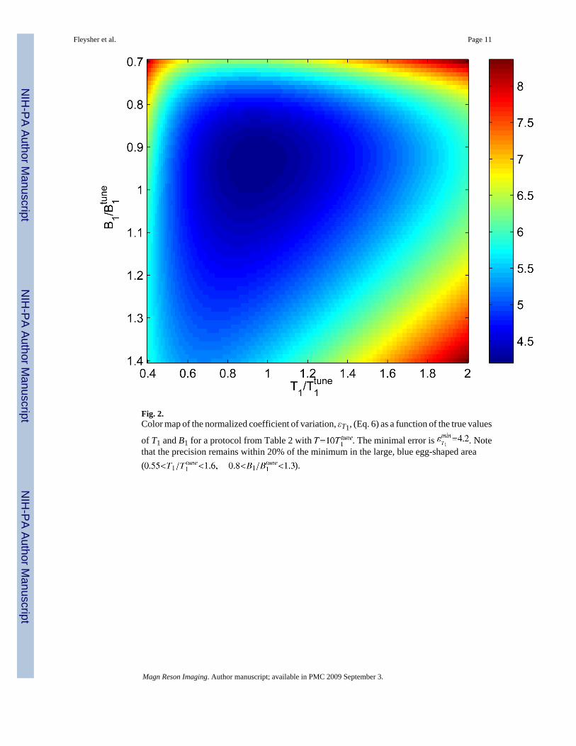
Fig. 2.Color map of the normalized coefficient of variation, εT1, (Eq. 6) as a function of the true values

of T1 and B1 for a protocol from Table 2 with . The minimal error is . Notethat the precision remains within 20% of the minimum in the large, blue egg-shaped area( ).

Fleysher et al.


NIH


NIH


NIH


Fig. 3.a: An axial T1 map in a cylindrical phantom acquired at 3×3×3 mm3 resolution. b: Histogramof the T1 values (jagged line) overlaid with a fitted Gaussian (solid line). Note that since thephantom is uniform the T1 map should be as well. To this end, the histogram features a narrowpeak at 294.5 ± 5.4 ms. c: Map of B1 showing that at the center region the flip angle is higherwhile towards the rim it is lower than nominal by up to 20%. d: B1-corrected -weighted spindensity (in arbitrary units) obtained using the reciprocity principle for the receive-transmit coil.

Fleysher et al.


NIH


NIH


NIH


Fig. 4.a: An axial T1 map in the same cylindrical phantom acquired using two-SPGR acquisition(without B1 correction). b: Histogram of the T1 values. Note that since the phantom is uniformthe non-uniformity of the T1 map and the width of the histogram are due to uncorrected B1inhomogeneity.

Fleysher et al.


NIH


NIH


NIH


Fig. 5.a: An axial T1 map in a human head at 1×1×1 mm3 resolution. b: Histogram of the T1 valuesfrom the slice exhibits a narrow peak at 950 ms corresponding predominantly to the whitematter. c: Map of B1 shows that at the center region the flip angle is higher while towards therim it is lower than nominal by about 15%. d: B1-corrected -weighted spin density (inarbitrary units) obtained using the reciprocity principle for the receive-transmit coil. In allpanels, black speckles represent pixels where the signals could not be described by Eq. (1)presumably due to intravoxel variations of T1 or motion.

Fleysher et al.


NIH


NIH


NIH


NIH


NIH


NIH


Fleysher et al.

Table 1Configuration of the brute-force search algorithm employed for sequence parameter optimization. The range of nominalflip angles was limited to (15°, 135°).

Experiment duration Minimum TRm Step in TRm Step in αm, (°)

T ≤ 2.0T1 0.01T1 0.01T1 5

T > 2.0T1 0.1T1 0.1T1 5


NIH


NIH


NIH


Fleysher et al. Ta

ble

2O

ptim

al S

PGR

seq

uenc

e pa

ram

eter

s fo

r T1

estim

atio

n fo

r a g

iven

tota

l im

agin

g tim

e T

and

. The

cor

resp

ondi

ng a

vera

ge n

orm

aliz

ed c

oeff

icie

nt o

f var

iatio

n is

als

o lis

ted.

Opt

imal

read

out d

urat

ion:

.

T∕T1tu

neε‒T1

TR1∕T1tu

neB 1tuneα 1

,( °

)N

1TR2∕T1tu

neB 1tuneα 2

,( °

)N

2TR3∕T1tu

neB 1tuneα 3

,( °

)N

3

0.1

20.6

648

0.03

151

0.03

351

0.04

135

1

0.2

14.1

786

0.06

151

0.05

401

0.09

135

1

0.3

12.3

081

0.09

151

0.04

352

0.13

135

1

0.4

11.3

185

0.11

151

0.04

353

0.17

135

1

0.5

10.7

166

0.13

151

0.05

403

0.22

135

1

0.6

10.3

048

0.14

151

0.05

404

0.26

135

1

0.7

10.0

273

0.16

151

0.05

405

0.29

135

1

0.8

9.83

080.

1715

10.

0540

60.

3313

51

0.9

9.67

180.

2115

10.

0540

60.

3913

51

1.0

9.52

400.

2215

10.

0540

70.

4313

51

1.1

9.39

590.

2215

10.

0545

80.

4813

51

1.2

9.27

050.

2315

10.

0545

90.

5213

51

1.3

9.13

710.

3020

10.

0540

90.

5513

51

1.4

8.99

330.

3120

10.

0540

100.

5913

51

1.5

8.86

220.

3220

10.

0540

110.

6313

51

1.6

8.72

720.

3320

10.

0540

110.

7213

51

1.7

8.59

480.

3420

10.

0540

120.

7613

51

1.8

8.45

800.

3520

10.

0540

120.

8513

51

1.9

8.32

220.

3420

10.

0545

130.

9113

51

2.0

8.18

080.

3620

10.

0540

130.

9913

51

3.0

6.97

890.

420

10.

155

91.

713

51

4.0

6.00

720.

420

10.

150

112.

512

01

5.0

5.39

750.

625

10.

150

152.

912

01

6.0

5.03

390.

930

10.

150

193.

212

51

7.0

4.80

821.

130

10.

150

233.

612

51

8.0

4.66

071.

335

10.

150

283.

912

51

9.0

4.57

091.

640

10.

150

324.

212

51


NIH


NIH


NIH


Fleysher et al.

T∕T1tu

neε‒T1

TR1∕T1tu

neB 1tuneα 1

,( °

)N

1TR2∕T1tu

neB 1tuneα 2

,( °

)N

2TR3∕T1tu

neB 1tuneα 3

,( °

)N

3

10.0

4.50

352.

250

10.

150

364.

213

01

11.0

4.43

963.

165

10.

150

394.

013

51

12.0

4.37

893.

470

10.

150

444.

213

51

13.0

4.33

703.

875

10.

150

494.

313

51

14.0

4.31

444.

075

10.

150

554.

513

51

15.0

4.30

554.

480

10.

150

604.

613

51

16.0

4.30

954.

580

10.

150

664.

913

51

17.0

4.32

484.

780

10.

150

744.

913

51

18.0

4.35

144.

980

10.

150

824.

913

51

19.0

4.38

854.

980

10.

150

924.

913

51

20.0

4.41

343.

985

20.

145

744.

813

51


TriTone: a radiofrequency field ( B 1)-insensitive T 1 estimator for MRI at high magnetic fields

Documents

Transcript of TriTone: a radiofrequency field ( B 1)-insensitive T 1 estimator for MRI at high magnetic fields