Monte Carlo-based tail exponent estimator

MONTE CARLO-BASED TAIL EXPONENT ESTIMATOR.

JOZEF BARUNIK* AND LUKAS VACHA**

Abstract. In this paper we propose a new approach to estimation of the tailexponent in financial stock markets. We begin the study with the finite sample be-havior of the Hill estimator under α−stable distributions. Using large Monte Carlosimulations we show that the Hill estimator overestimates the true tail exponentand can hardly be used on samples with small length. Utilizing our results, weintroduce a Monte Carlo-based method of estimation for the tail exponent. Ourproposed method is not sensitive to the choice of tail size and works well also onsmall data samples. The new estimator also gives unbiased results with symmet-rical confidence intervals. Finally, we demonstrate the power of our estimator onthe international world stock market indices. On the two separate periods of 2002–2005 and 2006–2009 we estimate the tail exponent.

JEL: C1, C13, C15, G0Keywords: Hill estimator, α-stable distributions, tail exponent estimation

* Corresponding author, Institute of Information Theory and Automation, Academy of Sci-ences of the Czech Republic, Institute of Economic Studies, Charles University, Prague, Email:[email protected].

** Institute of Information Theory and Automation, Academy of Sciences of the Czech Republic,Institute of Economic Studies, Charles University, Prague, Email: [email protected].

The authors would like to thank Martin Smid for many useful discussions and careful read-ing of the manuscript. Support from the Czech Science Foundation under Grants 402/09/0965,402/09/H045 and 402/08/P207 and from Ministry of Education MSMT 0021620841 is gratefullyacknowledged.

1

arX

iv:1

201.

4781

v1 [

q-fi

n.C

P] 2

3 Ja

n 20

12

MONTE CARLO-BASED TAIL EXPONENT ESTIMATOR. 2

1. Introduction

Statistical analysis of financial data has been of vigorous interest in recent years,mainly among the physics community (Mantegna and Stanley, 2000; Bouchaud andPotters, 2001; Buchanan, 2002; Mantegna et al., 1999; Plerou et al., 2000; Stanleyet al., 2000; Stanley, 2003). One of the main reasons driving the research is the useof established statistical characteristics to better describe and understand real-worldfinancial data.

Dynamics of financial markets is the outcome of large number of individual decisionsbased on heterogeneous information. Financial returns representing the interactionof the market participants have been assumed to be Normally distributed for a longtime. The strongest argument supporting this assumption is based on the Cen-tral Limit Theorem, which states that the sum of a large number of independent,identically distributed variables from a finite-variance distribution will tend to benormally distributed. However, financial returns showed to have heavier tails, whichis a possible source of infinite variance.

Mandelbrot (1963) and Fama (1965) proposed stable distributions as an alternativeto the Gaussian distribution model. Stable distributions were introduced by Levy(1925), who investigated the behavior of sums of independent random variables. Al-though we know other heavy-tailed alternative distributions (such as student’s t,hyperbolic or normal inverse Gaussian), stable distributions are attractive for re-searchers as they are supported by the generalized Central Limit Theorem. Thetheorem states that stable laws are the only possible limit distributions for properlynormalized and centered sums of independent, identically distributed random vari-ables. A sum of two independent random variables having a Levy stable distributionwith parameter α is again a Levy stable distribution with the same parameter α.However, this invariance property does not hold for different values of α. Observedstock market prices are argued to be the sum of many small terms, hence a stablemodel should be used to describe them. When α < 2, the variance of the stableprocess is infinite and the tails are asymptotically equivalent to a Pareto law, i.e.,they exhibit power-law behavior. Stable distributions have been proposed as a modelfor many types of physical and economic systems as they can accommodate fat tailsand asymmetry and fit the data well. Examples in finance and economics are givenin Mandelbrot (1963), Fama (1965), Embrechts et al. (1997) or Rachev and Mittnik(2000).

There have, however, been many applications of Levy stable distributions to empiri-cal data sets which could raise doubts about the correctness of the tail estimate (Lux,1996; Voit, 2005; Podobnik et al., 2000). There is a significant difference between the


value of the estimated α (based on the whole data set) and the estimated tail expo-nent. The tail exponent is estimated only on an arbitrarily chosen part of the data(Hill, 1975; Weron, 2001). Since extreme observations of prices on financial marketsare of great importance, this problem deserves further research. If α is underesti-mated, the occurrence of extreme events is overestimated. Weron (2001) shows thatthe estimated tail exponent is very sensitive to changes in parameters and to thesize of the data set, hence the estimates can be highly misleading. Simulations showthat a large data set (106) is needed for identification of the true tail behavior. Thelogical step is to use high-resolution data analysis. Lux (1996) was one of the firstto use high-frequency data, doing so for analysis of the German stock market index.Several studies concerning estimation of stable distributions followed (Mantegna andStanley, 2000; Dacorogna et al., 2001; Voit, 2005).

In our paper, we append an analysis of the finite sample properties of the Hill esti-mator to the discussions. Moreover, we introduce a Monte Carlo-based tail exponentestimation method. In the first part, we briefly discuss the basics of the Hill esti-mator as well as stable distributions and their tail behavior. In the second part, weprovide the finite sample properties of the Hill estimator and discuss the implicationsfor its use on real-world data. In the third part, we utilize the results and propose atail exponent estimation method based on Monte Carlo simulations. Finally, we il-lustrate the power of our method of estimation on leading world stock market indicesand conclude.

2. Estimation of the tail exponent

The simplest method of estimating the tail exponent α is log-log linear regression.This method is very sensitive to the sample size and the choice of the number ofobservations used in the regression. Weron (2001) shows that it also yields biasedestimates and cannot be used for financial applications. Popular method for esti-mating the tail exponent is also rank-frequency plot. Gabaix and Ibragimov (2009)proposed an extension of the rank-frequency plot with lower bias for small samples.Maximum likelihood method of estimation still belongs to most reliable techniques.For example Clauset et al. (2009) combine maximum-likelihood fitting with goodness-of-fit tests based on Kolmogorov-Smirnov statistic and likelihood ratios. Recently,many authors have studied the return intervals between consecutive price fluctuationsabove some volatility threshold. Podobnik et al. (2009) found a simple relationshipbetween the mean return intervals τq and the threshold q, τq ∝ qα, where α is power-law exponent. As authors show, this approach can also be used for estimation of thepower-law exponent for financial data.


Another widely used tail exponent estimator, equivalent to maximum-likelihood fit-ting, based on order statistics is proposed in Hill (1975). Pickands (1975) and Dekkerset al. (1989) show other variations of the Hill estimator. Mittnik et al. (1998) providea modification of the Pickands estimator using high-order approximation. A quantilemethod is used by McCulloch (1996). For more detailed discussion on tail estimatorssee Embrechts et al. (1997) and Resnick (2007).

The Hill estimator tends to overestimate the tail exponent of a stable distribution ifthe value of α is close to two and the sample size is not very large. For a more detaileddiscussion see Weron (2001) and Embrechts et al. (1997). Several researchers haveused misleading estimators of the tail exponent α to conclude that various data setshad α > 2, i.e., the data is not stable. First of all, let us briefly introduce the Hillestimator.

2.1. Hill estimator. The most popular method for estimating the tail exponentα is the Hill estimator (Hill, 1975). The Hill estimator is used to estimate thetail exponent only, therefore it does not assume a parametric form for the entiredistribution function.

Let’s suppose X1, X2, . . . , Xn is a sequence of i.i.d. random variables with the dis-tribution function F (x). Furthermore, let’s assume that 1 − F (x) has a regularlyvarying upper tail with coefficient −α.

(1) P (X > x) = 1− F (x) = x−αL(x), x > 0

where the function L(x) is slowly varying at infinity1 (for more details see Resnick(2007)).

Equation 1 indicates that the right tail of the distribution function F (x) has thesame asymptotic properties as the tail of the Pareto distribution, see (Wagner andMarsh, 2004).

Let us define the order statistics X(1) ≥ X(2) ≥ . . . ≥ X(n). The Hill estimator of thetail exponent α is defined as:

(2) αH =

(1

k

k∑i=1

logX(n−i+1) − logX(n−k)

)−1,

where k is a truncation (or smoothing) parameter which defines a subsample usedfor the estimation, k < n.

1If eq. 1 is satisfied, the distribution function F (x) belongs to the maximum domain of attractionof φα, F ∈ MDA(φα), where φα(x) = e−x

α

, x > 0, α > 0. For a more detailed treatment of theextreme value theory see Embrechts et al. (1997)


Many authors have studied the asymptotical properties of the Hill estimator. Ac-cording to Mason (1982) the Hill estimator is weakly consistent if

(3) k →∞, k

n→ 0 as n→∞.

Furthermore, Goldie and Smith (1987) proved the asymptotic normality of the Hillestimator, i.e.,

(4)√k(α−1H − α

−1) ∼ N(0, α−2).

Consequently, αH is also approximately normal with mean α and variance α2/k.Moreover, (Hsing, 1991) shows that the Hill estimator is asymptotically quite robustwith respect to deviations from independence. For a more detailed discussion of theproperties of the Hill estimator see Resnick (2007), Embrechts et al. (1997).

2.2. Choice of optimal k in the Hill estimator. In the classical approach, thereis considerable difficulty in choosing the right value of the truncation parameter k,since it can influence the accuracy of the estimate significantly. The methods ofchoosing k from the empirical data set are very often based on a trade-off betweenthe bias and the variance of the Hill estimator. k has to be sufficiently small to ensurethe observations X(1) ≥ X(2) ≥ . . . ≥ X(k) still belong to the tail of the distribution.On the other hand, if k is too small, the estimator lacks precision.

There are several methods for choosing the “optimal” value of k. The first possibilityis to make a Hill plot, where αH is plotted against k, and look for a region where thegraph has fairly stable behavior to identify the optimal value of the order statisticsk. Alternatively, there are other methods for choosing the optimal k, such as thebootstrap approach (Hall, 1990).

In our simulations later in this paper we show that choosing k from the Hill plotis very inaccurate and for higher values of α it is almost impossible to set its rightvalue. Resnick (2007) clearly illustrates why this technique very often leads to a “Hillhorror plot” from which it is not possible to discern the correct value of k. Using theHill estimates from simulated random variables on a standard symmetric Levy-stabledistribution for different values of k, we also clearly demonstrate that choosing the“correct” k is a very difficult task. Furthermore, for a short dataset (< 106) it isusually impossible to find out the right value of k, especially when α is close to 2.Unfortunately, this setting is very often the case when we analyze empirical financialmarket data.

To overcome the problem of choosing the optimal k we introduce a new estimationmethod based on comparison of the estimate of the empirical dataset with estimates


on a pre-simulated random variable from the standard Levy distribution for k on theinterval [1%− 20%]. The main advantage of our approach is that it does not assumethe smoothing parameter k to be known.

3. Finite sample properties of the Hill estimator for differentheavy tails

We would like to study the finite sample behavior of the Hill estimator in detail forstable distributions with different heavy tails first. Let us start with an introductionto stable distributions.

3.1. Stable distributions. Stable distributions are a class of probability laws withappealing theoretical properties. Their application to financial modeling comes fromthe fact that they generalize the Gaussian distribution, which does not describe well-known stylized facts about stock market data. Stable distributions allow for heavytails and skewness. In this paper, we provide a basic idea about stable distributions.Interested readers can find the theorems and proofs in Nolan (2003), Zolotarev (1986)and Samorodnitsky and Taqqu (1994).

The reason for the term stable is that stable distributions retain their shape up toscale and shift under addition: if X, X1, X2,..., Xn are independent, identicallydistributed stable random variables, then for every n

(5) X1 +X2 + ...+Xnd= cnX + dn

for constants cn > 0 and dn. Equality (d=) here means that the right-hand and left-

hand sides have the same distribution. Normal distributions satisfy this property:the sum of normals is normal. In general, the class of all laws satisfying (5) can bedescribed by four parameters, (α, β, γ, δ). Parameter α is called the characteristicexponent and must be in the range α ∈ (0, 2]. The coefficients cn are equal to n1/α.Parameter β is called the skewness of the law and must be in the range −1 ≤ β ≤ 1.If β = 0, the distribution is symmetric, if β > 0 it is skewed to the right, and ifβ < 0 it is skewed to the left. While parameters α and β determine the shape of thedistribution, γ and δ are scale and location parameters, respectively.

Due to a lack of closed form formulas for probability density functions (except forthree stable distributions: Gaussian, Cauchy, and Levy) the α-stable distributioncan be described by a characteristic function which is the inverse Fourier transformof the probability density function, i.e., φ(u) = E exp(iuX).

A confusing issue with stable parameters is that there are multiple parametrizationsused in the literature. Nolan (2003) provides a good guide to all the definitions. In


this paper, we will use Nolan’s parametrization, which is jointly continuous in allfour parameters. A random variable X is distributed by S(α, β, γ, δ) if it has thefollowing characteristic function:

(6) φ(u) =

{exp(−γα|u|α[1 + iβ(tan πα

2 )(signu)(|γu|1−α − 1)] + iδu) α 6= 1exp(−γ|u|[1 + iβ 2

π (signu) ln(γ|u|)] + iδu) α = 1

There are only three cases where a closed-form expression for density exists andwe can verify directly if the distribution is stable – the Gaussian, Cauchy, andLevy distributions. Gaussian laws are stable with α = 2 and β = 0. More pre-cisely, N(0, σ2) = S(2, 0, σ/

√2, 0). Cauchy laws are stable with α = 1 and β = 0,

Cauchy(γ, δ) = S(1, 0, γ, δ); and finally, Levy laws are stable with α = 1/2 and β = 1;Levy(γ, δ) = S(1/2, 1, γ, γ + δ). Nolan (2003) shows these examples in detail.

For all values of parameter α < 2 and −1 < β < 1, stable distributions havetwo tails that are asymptotically power laws. The asymptotic tail behavior of non-Gaussian stable laws for X ∼ S(α, β, γ, δ) with α < 2 and −1 < β < 1 is defined asfollows:

limx→∞

xαP (X > x) = cα (1 + β) γα(7)

limx→∞

xαP (X < −x) = cα (1− β) γα,(8)

where

(9) cα = sin(πα

2

)Γ (α) /π.

If the data is stable, the empirical distribution function should be approximately astraight line with slope −α in a log-log plot.

A negative aspect of non-Gaussian stable distributions (α < 2) is that not all mo-ments exist.2 The first moment EX is not finite (or is undefined) when α ≤ 1. Onthe other hand, when 1 < α ≤ 2 the first moment is defined as

(10) EX = µ = δ − βγ tanπα

2.

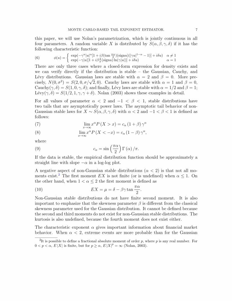
Non-Gaussian stable distributions do not have finite second moment. It is alsoimportant to emphasize that the skewness parameter β is different from the classicalskewness parameter used for the Gaussian distribution. It cannot be defined becausethe second and third moments do not exist for non-Gaussian stable distributions. Thekurtosis is also undefined, because the fourth moment does not exist either.

The characteristic exponent α gives important information about financial marketbehavior. When α < 2, extreme events are more probable than for the Gaussian

2It is possible to define a fractional absolute moment of order p, where p is any real number. For0 < p < α, E |X| is finite, but for p ≥ α, E |X|p =∞ (Nolan, 2003).


distribution. From an economic point of view some values of parameter α do notmake sense. For example, in the interval 0 < α < 1 the random variable X doesnot have a finite mean. In this case, an asset with returns which follow a stable lawwith 0 < α < 1 would have an infinite expected return. Thus, we are looking for1 < α < 2 to be able to predict extreme values more precisely than by the Gaussiandistribution.

3.2. Research design. The simulations are constructed so as to show how the Hillestimator behaves for different heavy tails data. For this purpose we use the Levy sta-ble distribution depending on parameters (α, β, γ, δ) and set them to (α, 0,

√2/2, 0),

where 1.1 ≤ α ≤ 2 with a step of 0.1. For each parameter α, 1,000 time series withlengths from 103 to 106 are simulated and the tail exponent is estimated using theHill estimator for k ≤ 1% and k ∈ (1%, 20%] separately.

In other words, we simulate the grid of different α for different series lengths. Foreach position in the grid, we estimate the tail exponent using the Hill estimator.This allows us to study the finite sample properties of the Hill estimator for differentlength series, different tail exponents and different k.

3.3. Results from Monte Carlo simulations. The biggest problem with the op-timal choice of k is that α is not known, so we cannot really choose the optimal k.In our simulation, we show the finite sample properties of the Hill estimator k ≤ 1%and k ∈ (1%, 20%] separately.

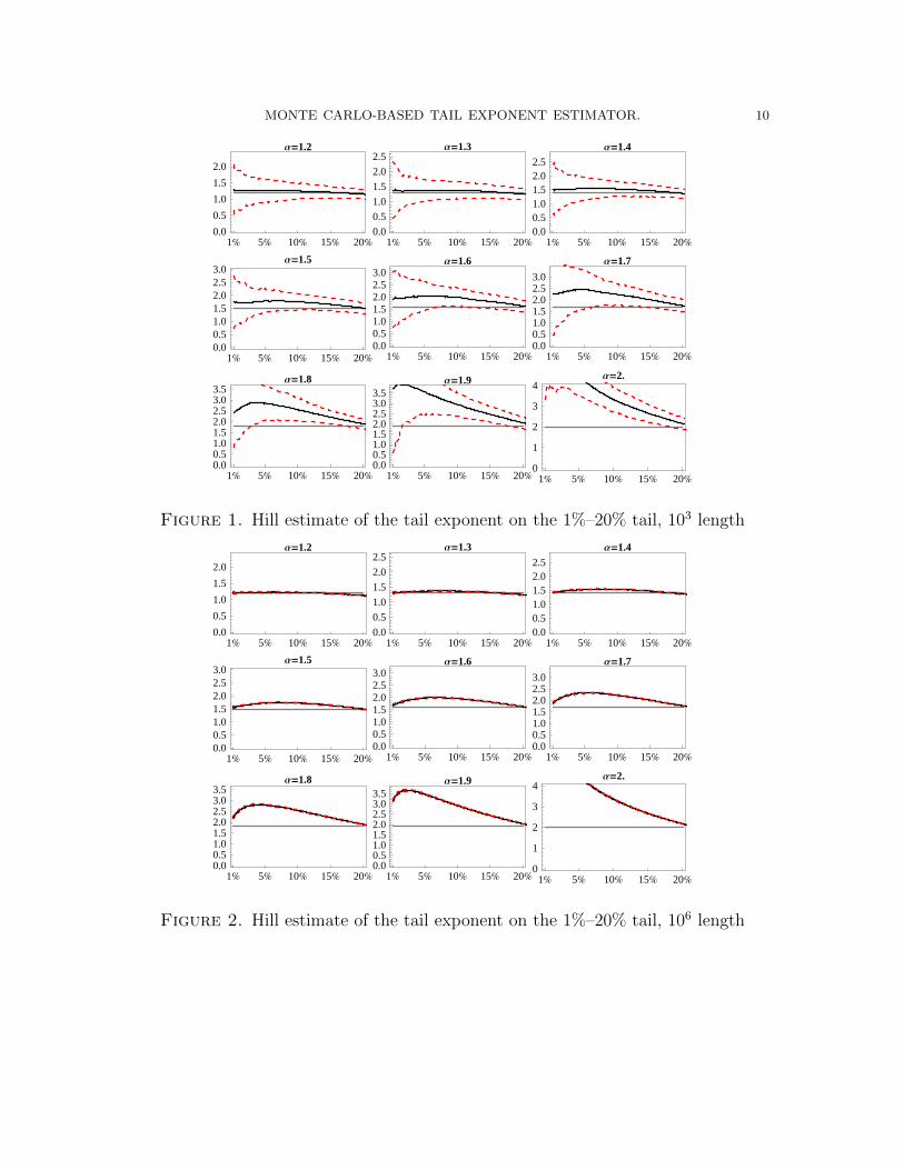
3.3.1. Hill estimation for k > 1%. We begin the simulations with a time series lengthof 103, which is a usual sample length for real-world financial data, i.e., it equates toapproximately 4 years of daily returns of a stock. Figure 1 shows the 95% confidenceintervals3 of the Hill estimate for different α for all k. It can be seen that it is verydifficult to statistically distinguish between different tail exponents α and it is veryunclear which optimal k we should choose.

Figure 2 shows much more precise results for a time series of length 106. This allowsfor narrow confidence intervals, but even with this exact result we can see that theHill estimator is problematic as it overestimates the value of the tail exponent andwe cannot pick the optimal k even from this large grid of simulated data. The onlyway of estimating the tail exponent would be to pick k, estimate the tail exponent,and compare it to the grid of simulated confidence intervals. But we would still needat least a 106 sample size to achieve an exact result. As we can see in Figure 1, wecannot get a statistically significant estimate on data with length 103. Table 1 shows

3All confidence intervals are computed from the asymptotic normality of the sample.


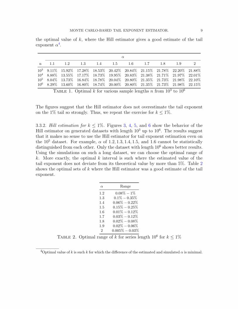
the optimal value of k, where the Hill estimator gives a good estimate of the tailexponent α4.

α

n 1.1 1.2 1.3 1.4 1.5 1.6 1.7 1.8 1.9 2

103 9.11% 15.92% 17.28% 18.53% 20.42% 20.84% 21.15% 21.78% 22.20% 21.88%104 8.88% 13.55% 17.17% 18.73% 19.95% 20.83% 21.38% 21.71% 21.97% 22.01%105 8.04% 13.73% 16.84% 18.78% 20.04% 20.80% 21.35% 21.73% 21.98% 22.10%106 8.29% 13.60% 16.80% 18.74% 20.00% 20.80% 21.35% 21.73% 21.98% 22.15%

Table 1. Optimal k for various sample lengths n from 103 to 106

The figures suggest that the Hill estimator does not overestimate the tail exponenton the 1% tail so strongly. Thus, we repeat the exercise for k ≤ 1%.

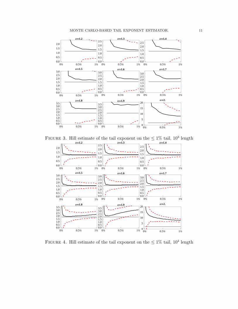
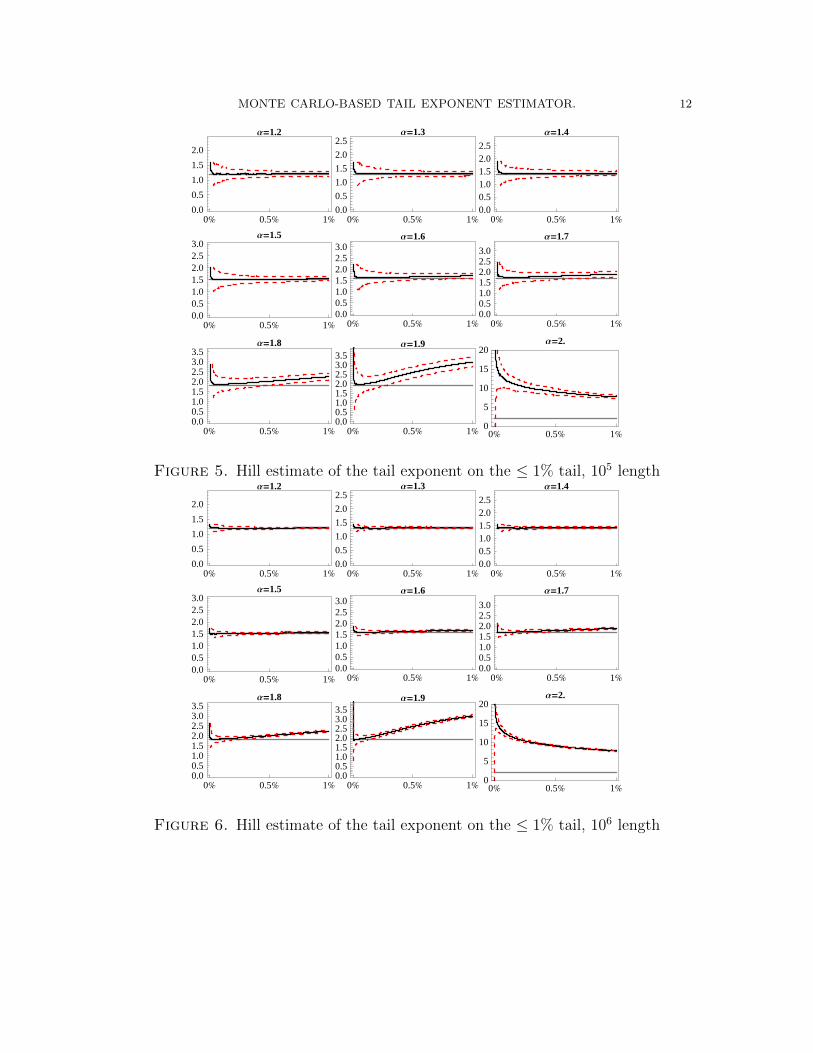
3.3.2. Hill estimation for k ≤ 1%. Figures 3, 4, 5, and 6 show the behavior of theHill estimator on generated datasets with length 103 up to 106. The results suggestthat it makes no sense to use the Hill estimator for tail exponent estimation even onthe 105 dataset. For example, α of 1.2, 1.3, 1.4, 1.5, and 1.6 cannot be statisticallydistinguished from each other. Only the dataset with length 106 shows better results.Using the simulations on such a long dataset, we can choose the optimal range ofk. More exactly, the optimal k interval is such where the estimated value of thetail exponent does not deviate from its theoretical value by more than 5%. Table 2shows the optimal sets of k where the Hill estimator was a good estimate of the tailexponent.

α Range

1.2 0.08%− 1%1.3 0.1%− 0.35%1.4 0.06%− 0.22%1.5 0.15%− 0.25%1.6 0.01%− 0.12%1.7 0.03%− 0.12%1.8 0.02%− 0.08%1.9 0.02%− 0.06%2 0.005%− 0.03%

Table 2. Optimal range of k for series length 106 for k ≤ 1%

4Optimal value of k is such k for which the difference of the estimated and simulated α is minimal.


1% 5% 10% 15% 20%

0.0

0.5

1.0

1.5

2.0

Α=1.2

1% 5% 10% 15% 20%

0.0

0.5

1.0

1.5

2.0

2.5Α=1.3

1% 5% 10% 15% 20%

0.00.51.01.52.02.5

Α=1.4

1% 5% 10% 15% 20%

0.00.51.01.52.02.53.0

Α=1.5

1% 5% 10% 15% 20%

0.00.51.01.52.02.53.0

Α=1.6

1% 5% 10% 15% 20%

0.00.51.01.52.02.53.0

Α=1.7

1% 5% 10% 15% 20%

0.00.51.01.52.02.53.03.5

Α=1.8

1% 5% 10% 15% 20%

0.00.51.01.52.02.53.03.5

Α=1.9

1% 5% 10% 15% 20%

0

1

2

3

4Α=2.

Figure 1. Hill estimate of the tail exponent on the 1%–20% tail, 103 length

1% 5% 10% 15% 20%

0.0

0.5

1.0

1.5

2.0

Α=1.2

1% 5% 10% 15% 20%

0.0

0.5

1.0

1.5

2.0

2.5Α=1.3

1% 5% 10% 15% 20%

0.00.51.01.52.02.5

Α=1.4

1% 5% 10% 15% 20%

0.00.51.01.52.02.53.0

Α=1.5

1% 5% 10% 15% 20%

0.00.51.01.52.02.53.0

Α=1.6

1% 5% 10% 15% 20%

0.00.51.01.52.02.53.0

Α=1.7

1% 5% 10% 15% 20%

0.00.51.01.52.02.53.03.5

Α=1.8

1% 5% 10% 15% 20%

0.00.51.01.52.02.53.03.5

Α=1.9

1% 5% 10% 15% 20%

0

1

2

3

4Α=2.

Figure 2. Hill estimate of the tail exponent on the 1%–20% tail, 106 length


0% 0.5% 1%

0.0

0.5

1.0

1.5

2.0

Α=1.2

0% 0.5% 1%

0.0

0.5

1.0

1.5

2.0

2.5Α=1.3

0% 0.5% 1%

0.00.51.01.52.02.5

Α=1.4

0% 0.5% 1%

0.00.51.01.52.02.53.0

Α=1.5

0% 0.5% 1%

0.00.51.01.52.02.53.0

Α=1.6

0% 0.5% 1%

0.00.51.01.52.02.53.0

Α=1.7

0% 0.5% 1%

0.00.51.01.52.02.53.03.5

Α=1.8

0% 0.5% 1%

0.00.51.01.52.02.53.03.5

Α=1.9

0% 0.5% 1%

0

5

10

15

20Α=2.

Figure 3. Hill estimate of the tail exponent on the ≤ 1% tail, 103 length

0% 0.5% 1%

0.0

0.5

1.0

1.5

2.0

Α=1.2

0% 0.5% 1%

0.0

0.5

1.0

1.5

2.0

2.5Α=1.3

0% 0.5% 1%

0.00.51.01.52.02.5

Α=1.4

0% 0.5% 1%

0.00.51.01.52.02.53.0

Α=1.5

0% 0.5% 1%

0.00.51.01.52.02.53.0

Α=1.6

0% 0.5% 1%

0.00.51.01.52.02.53.0

Α=1.7

0% 0.5% 1%

0.00.51.01.52.02.53.03.5

Α=1.8

0% 0.5% 1%

0.00.51.01.52.02.53.03.5

Α=1.9

0% 0.5% 1%

0

5

10

15

20Α=2.



0% 0.5% 1%

0.0

0.5

1.0

1.5

2.0

Α=1.2

0% 0.5% 1%

0.0

0.5

1.0

1.5

2.0

2.5Α=1.3

0% 0.5% 1%

0.00.51.01.52.02.5

Α=1.4

0% 0.5% 1%

0.00.51.01.52.02.53.0

Α=1.5

0% 0.5% 1%

0.00.51.01.52.02.53.0

Α=1.6

0% 0.5% 1%

0.00.51.01.52.02.53.0

Α=1.7

0% 0.5% 1%

0.00.51.01.52.02.53.03.5

Α=1.8

0% 0.5% 1%

0.00.51.01.52.02.53.03.5

Α=1.9

0% 0.5% 1%

0

5

10

15

20Α=2.


0% 0.5% 1%

0.0

0.5

1.0

1.5

2.0

Α=1.2

0% 0.5% 1%

0.0

0.5

1.0

1.5

2.0

2.5Α=1.3

0% 0.5% 1%

0.00.51.01.52.02.5

Α=1.4

0% 0.5% 1%

0.00.51.01.52.02.53.0

Α=1.5

0% 0.5% 1%

0.00.51.01.52.02.53.0

Α=1.6

0% 0.5% 1%

0.00.51.01.52.02.53.0

Α=1.7

0% 0.5% 1%

0.00.51.01.52.02.53.03.5

Α=1.8

0% 0.5% 1%

0.00.51.01.52.02.53.03.5

Α=1.9

0% 0.5% 1%

0

5

10

15

20Α=2.



In order to estimate the true tail exponent, we need a dataset with length of atleast 106, otherwise inference of the tail exponent may be strongly misleading andrejection of the Levy stable regime not appropriate. For the sake of clarity we haveto note that the results for the α = 2 should be interpreted with caution as it is thespecial case of Gaussian distribution which does not have heavy tails. Thus the Hillestimator is not appropriate in this case.

In the next section, we develop a Monte Carlo-based tail exponent estimator whichdeals with all of these problems.

4. Tail exponent estimator based on Monte Carlo simulations

After the study of the finite sample properties of the Hill estimator, we utilize theresults and introduce our Monte Carlo-based estimator. The Monte Carlo techniqueprovides an attractive method of building exact tests from statistics whose finitesample distribution is intractable but can be simulated, thus it can be utilized in ourproblem.

We construct our Monte Carlo-based tail exponent estimator as follows.

(1) Generate 1,000 i.i.d. α−stable distributed random variables Xα0 of lengthn, i.e. xα0

1 , xα02 , . . . , x

α0n ∼ S(α0, 0,

√2/2, 0), for each α0 parameter from the

range [1.01, 2] with step 0.01.

(2) For each Xα0 , estimate the tail exponent using the Hill estimator for all kfrom the interval (1%− 20%), i.e. αα0,k.

(3) From Monte Carlo simulations compute the expected value E[αα0,k] of theHill estimator for all k and all α0.

(4) Using the Hill estimator estimate the tail exponent αemp,k on an empiricaldataset of length n for all k from the interval (1%− 20%).

(5) Our Monte Carlo-based estimator αMC is defined as:

(11) αMC = arg minα0∈[1.01,2]

∑k

|αemp,k − E[αα0,k]|

In other words, we simulate random variables X of length n for 100 different α’s(representing the tail parameter) 1,000 times.5 On these random variables we esti-mate the tail exponent using the Hill estimator on the (1%− 20%) tail (as we have

5A more exact confidence interval can be obtained by generating more random variables


1 1.2 1.4 1.6 1.8 2

1.0

1.2

1.4

1.6

1.8

2.0

1.0

1.2

1.4

1.6

1.8

2.0

Α

Α`

H

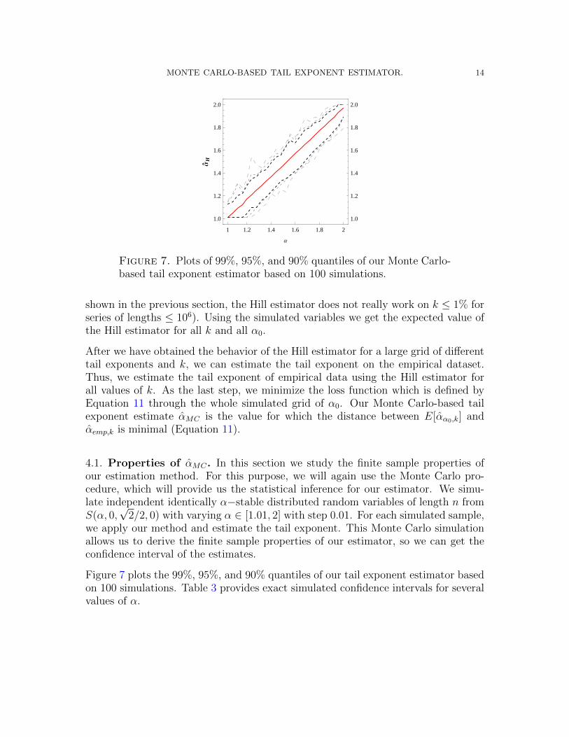
Figure 7. Plots of 99%, 95%, and 90% quantiles of our Monte Carlo-based tail exponent estimator based on 100 simulations.

shown in the previous section, the Hill estimator does not really work on k ≤ 1% forseries of lengths ≤ 106). Using the simulated variables we get the expected value ofthe Hill estimator for all k and all α0.

After we have obtained the behavior of the Hill estimator for a large grid of differenttail exponents and k, we can estimate the tail exponent on the empirical dataset.Thus, we estimate the tail exponent of empirical data using the Hill estimator forall values of k. As the last step, we minimize the loss function which is defined byEquation 11 through the whole simulated grid of α0. Our Monte Carlo-based tailexponent estimate αMC is the value for which the distance between E[αα0,k] andαemp,k is minimal (Equation 11).

4.1. Properties of αMC. In this section we study the finite sample properties ofour estimation method. For this purpose, we will again use the Monte Carlo pro-cedure, which will provide us the statistical inference for our estimator. We simu-late independent identically α−stable distributed random variables of length n fromS(α, 0,

√2/2, 0) with varying α ∈ [1.01, 2] with step 0.01. For each simulated sample,

we apply our method and estimate the tail exponent. This Monte Carlo simulationallows us to derive the finite sample properties of our estimator, so we can get theconfidence interval of the estimates.

Figure 7 plots the 99%, 95%, and 90% quantiles of our tail exponent estimator basedon 100 simulations. Table 3 provides exact simulated confidence intervals for severalvalues of α.


0.5% 2.5% 5% αMC 95% 97.5% 99.5%

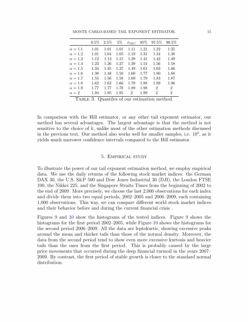
α = 1.1 1.01 1.01 1.01 1.11 1.21 1.22 1.25α = 1.2 1.01 1.04 1.05 1.19 1.31 1.34 1.38α = 1.3 1.12 1.13 1.15 1.29 1.41 1.42 1.49α = 1.4 1.23 1.26 1.27 1.39 1.54 1.56 1.58α = 1.5 1.34 1.35 1.37 1.49 1.61 1.63 1.66α = 1.6 1.38 1.48 1.50 1.60 1.77 1.80 1.88α = 1.7 1.55 1.56 1.58 1.69 1.79 1.83 1.87α = 1.8 1.62 1.62 1.66 1.79 1.88 1.89 1.96α = 1.9 1.77 1.77 1.78 1.89 1.98 2 2α = 2 1.94 1.95 1.95 2 1.99 2 2

Table 3. Quantiles of our estimation method.

In comparison with the Hill estimator, or any other tail exponent estimator, ourmethod has several advantages. The largest advantage is that the method is notsensitive to the choice of k, unlike most of the other estimation methods discussedin the previous text. Our method also works well for smaller samples, i.e. 103, as ityields much narrower confidence intervals compared to the Hill estimator.

5. Empirical study

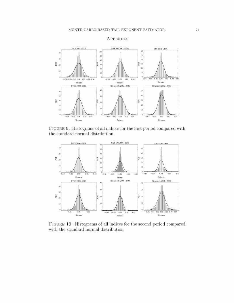
To illustrate the power of our tail exponent estimation method, we employ empiricaldata. We use the daily returns of the following stock market indices: the GermanDAX 30, the U.S. S&P 500 and Dow Jones Industrial 30 (DJI), the London FTSE100, the Nikkei 225, and the Singapore Straits Times from the beginning of 2002 tothe end of 2009. More precisely, we choose the last 2,000 observations for each indexand divide them into two equal periods, 2002–2005 and 2006–2009, each containing1,000 observations. This way, we can compare different world stock market indicesand their behavior before and during the current financial crisis .

Figures 9 and 10 show the histograms of the tested indices. Figure 9 shows thehistograms for the first period 2002–2005, while Figure 10 shows the histograms forthe second period 2006–2009. All the data are leptokurtic, showing excessive peaksaround the mean and thicker tails than those of the normal density. Moreover, thedata from the second period tend to show even more excessive kurtosis and heaviertails than the ones from the first period. This is probably caused by the largeprice movements that occurred during the deep financial turmoil in the years 2007–2009. By contrast, the first period of stable growth is closer to the standard normaldistribution.


We use our Monte Carlo method to estimate the tail exponents for all the datasets.Before we start the estimations, we set the length n of the simulated series from ouralgorithm to 1,000 so that it corresponds to the length of the empirical dataset andwe can statistically compare the estimates. Table 4 shows the tail exponent estimateswith confidence intervals. Let us further demonstrate the estimation method on the

Empirical Confidence Intervals

0.5% 2.5% 5% αMC 95% 97.5% 99.5%

German DAX 30 2002–2005 1.50 1.53 1.55 1.64 1.77 1.8 1.852006–2009 1.47 1.53 1.56 1.70 1.79 1.81 1.87

U.S. S&P500 2002–2005 1.53 1.57 1.58 1.74 1.85 1.88 1.942006–2009 1.35 1.38 1.4 1.54 1.63 1.70 1.72

U.S. DJI 30 2002–2005 1.50 1.53 1.55 1.69 1.83 1.87 1.892006–2009 1.29 1.38 1.4 1.54 1.66 1.70 1.77

London FTSE 100 2002–2005 1.34 1.42 1.43 1.57 1.69 1.69 1.712006–2009 1.50 1.55 1.55 1.69 1.82 1.87 1.91

Japan Nikkei 225 2002–2005 1.79 1.81 1.84 1.93 1.98 2 22006–2009 1.58 1.60 1.62 1.77 1.88 1.89 1.89

Singapore Straits 2002–2005 1.72 1.72 1.74 1.85 1.94 1.95 1.972006–2009 1.47 1.50 1.52 1.66 1.78 1.81 1.87

Table 4. Exact confidence intervals (quantiles) of the estimated tailexponent α.

1% 5% 10% 15% 20%

1

2

3

4

Α=1.55

1% 5% 10% 15% 20%

1

2

3

4

5

Α=1.69

1% 5% 10% 15% 20%

1

2

3

4

5

Α=1.87

Figure 8. Plot of Hill estimates through different k for the FTSEindex (second period of 2006–2009) for α = 1.55, α = 1.69, and α =1.87, which are our αMC with the 0.025% and 97.5% quantiles.

example of the London FTSE 100 index for the second period. Figure 8 plots theempirical Hill estimates through different k and compares them to 1,000 simulationsof α = 1.55, α = 1.69, and α = 1.87 (these are our Monte Carlo estimates withthe 0.025% and 97.5% quantiles). It is immediately visible from the plots that the


loss function defined in our estimation algorithm reaches its minimum for α = 1.69.We plot another two cases just for illustration of what our estimate looks like at thecritical levels. After minimizing the loss function and choosing the tail exponent, wederive the finite sample properties of the estimate. From Table 4, we can see that1.55 and 1.87 are the 0.025% and 97.5% quantiles.

Unlike the classical Hill estimation procedure, we can see that our method is notsensitive to the choice of k. Moreover, it is a much stronger result for the tailexponent, as it accounts for all possible k’s, not only the one chosen. Using theclassical Hill estimation procedure, we would select k and compute the tail exponent,but as we discussed in the previous text, there is always a trade-off between bias andvariance when choosing the optimal k. Our method reduces this problem. Finally,the sample on which we estimate the tail exponent is quite small. In previous sectionswe showed that Hill estimation does not work well for such small samples, but ourmethod works fine.

6. Conclusion

In this paper, we have researched the finite sample behavior of the Hill estimatorunder α−stable distributions and we introduce a Monte Carlo-based method of es-timation for the tail exponent.

First of all, we provide Monte Carlo confidence intervals for the Hill estimator underdifferent α’s and k on the interval k ∈ (0, 20%] of sample size 103 up to 106. We alsoprovide the optimal range of k for the series length 106. Based on our simulations, weconclude that in order to estimate the true tail exponent using the Hill estimator, weneed a dataset of at least 106 length, i.e., high frequency data, otherwise inference ofthe tail exponent may be strongly misleading and rejection of the Levy stable regimenot appropriate.

In the second part of the paper, we utilize the results and introduce a tail exponentprocedure based on Monte Carlo simulations. It is based on the idea of simulatinga large grid of random variables from the Levy stable distribution with different αexponents and estimating the tail exponent using the Hill estimator for all differentk. After obtaining the behavior of the Hill estimator on this large grid of different tailexponents and k, all we need to do is to estimate the tail exponent on the empiricaldataset for all k’s and compare all the values with the simulated grid. Using thisalgorithm we get estimates of the tail exponent.

In comparison with the Hill estimator, or any other tail exponent estimator, ourmethod has several advantages. The largest advantage is that it is not sensitive


to the choice of k. Moreover, the method works well for small samples. The newestimator gives unbiased results with symmetrical confidence intervals.

Finally, we illustrate the power of our tail exponent estimation method on an empir-ical dataset. We use daily returns of leading world stock markets: the German DAX,the U.S. S&P 500 and Dow Jones Industrial (DJI), the London FTSE, the Nikkei225, and the Singapore Straits Times from the beginning of 2002 to the end of 2009.We divide this period into two equal sub-periods and compare the tail exponentsestimated using our method.

References

Bouchaud, J. P. and M. Potters (2001). Theory of Financial Risks: From StatisticalPhysics to Risk Management. Cambridge: Cambridge University Press.

Buchanan, M. (2002). The physics on the trading floor. Nature 10-12 (415).

Clauset, A., C. R. Shalizi, and M. E. J. Newman (2009). Power-law distributions inempirical data. SIAM Review 51 (4), 661–703.

Dacorogna, M., R. Gencay, U. Mueller, and O. Pictet (2001). An Introduction toHigh-Frequency finance. Academic press.

Dekkers, A. L. M., J. H. J. Einmahl, and L. De Haan (1989). A moment estimatorfor the index of an extreme-value distribution. The Annals of Statistics 17 (4),1833–1855.

Embrechts, P., C. Kluppelberg, and T. Mikosch (1997). Modelling Extremal Eventsfor Insurance and Finance. Heidelberg: Springer Verlag.

Fama, E. (1965). The behavior of stock prices. Journal of Business (38), 34–105.

Gabaix, X. and R. Ibragimov (2009). Rank1/2: A simple way to improve theols estimation of tail exponents. Journal of Business and Economic Statis-tics (doi:10.1198/jbes.2009.06157).

Goldie, C. M. and R. L. Smith (1987). Slow variation with remainder: Theory andapplications. Quarterly Journal of Mathematics, Oxford 2nd Series 38 (1), 45–71.

Hall, P. (1990). Using the bootstrap to estimate mean squared error and selectsmoothing parameters in nonparametric probles. Journal of Multivariate Analy-sis 32 (2), 177–203.


Hill, B. M. (1975). A simple general approach to inference about the tail of adistribution. The Annals of Statistics 3 (5), 1163–1174.

Hsing, T. (1991). On tail index estimation using dependent data. Annals of Statis-tics 19 (3), 1547–1569.

Levy, P. (1925). Calcul des Probabilites. Gauthier Villars.

Lux, T. (1996). The stable paretian hypothesis and the frequency of large returns.Applied Financial Economics 6, 463–475.

Mandelbrot, B. (1963). The variation of certain speculative prices. Journal of Busi-ness (26), 394–419.

Mantegna, R., Z. Palagyi, and H. Stanley (1999). Applications of statistical mechan-ics to finance. Physica A 274 (1-2), 216–221.

Mantegna, R. and H. Stanley (2000). An Introduction to Econophysics. Cambridge:Cambridge University Press.

Mason, D. M. (1982). Laws of large numbers for sums of extreme values. Annals ofProbability 10 (3), 754–764.

McCulloch, J. H. (1996). Financial applications of stable distributions (Handbookof Statistics ed.), Volume 14. Elsevier.

Mittnik, S., P. M. S., and S. T. Rachev (1998). A tail estimator for the indexof the stable paretian distribution. Communications in statistics. Theory andmethods 27 (5), 1239–1262.

Nolan, J. P. (2003). Stable Distributions: Models for Heavy Tailed Data. Boston,MA: Birkhauser.

Pickands, J. (1975). Statistical inference using extreme order statistics. Annals ofStatistics 3 (1), 119–131.

Plerou, V., P. Gopikrishnan, B. Rosenow, L. A. N. Amaral, and H. E. Stanley (2000).A random matrix theory approach to financial cross-corelations. Physica A 287 (3-4), 374–382.

Podobnik, B., D. Horvatic, A. M. Petersen, and H. E. Stanley (2009). Cross-correlations between volume change and price change. Proceedings of the NationalAcademy of Sciences 106 (52), 22079–22084.

Podobnik, B., P. C. Ivanov, Y. Lee, and H. E. Stanley (2000). Scale-invariant trun-cated levy process. Europhysics Letters 52 (5), 491.


Rachev, S. T. and S. Mittnik (2000). Stable Paretian Models in Finance. New York:Wiley.

Resnick, S. I. (2007). Heavy Tail Phenomena: Probabilistic and Statistical Model-ing. Springer Series in Operations Research and Financial Engineering. New York:Springer.

Samorodnitsky, G. and M. S. Taqqu (1994). Stable Non-Gaussian Random Processes.New York: Chapman and Hall.

Stanley, H. (2003). Statistical physics and economic fluctuations: do outliers exist?Physica A 318 (1-2), 279–292.

Stanley, H., L. Amaral, P. Gopikrishnan, and V. Plerou (2000). Scale invariance anduniversality of economic fluctuations. Physica A 283 (1-2), 31–41.

Voit, J. (2005). The Statistical Mechanics of Financial Markets. Heidelberg:Springer-Verlag Berlin.

Wagner, N. and T. A. Marsh (2004). Tail index estimation in small smaples sim-ulation results for independent and arch-type financial return models. StatisticalPapers 45 (4), 545–561.

Weron, R. (2001). Levy-stable distributions revisited: Tail index > 2 does notexclude the levy-stable regime. International Journal of Modern Physics C 12,209–223.

Zolotarev, V. M. (1986). One-Dimensional Stable Distributions, Volume 65 of Amer.Math. Soc. Transl. of Math. Monographs. Providence, RI: Amer. Math. Soc.


Appendix

-0.06 -0.04 -0.02 0.00 0.02 0.04 0.060

10

20

30

40

Returns

PDF

DAX 2002-2005

-0.04 -0.02 0.00 0.02 0.040

10

20

30

40

50

60

Returns

PDF

S&P 500 2002-2005

-0.06 -0.04 -0.02 0.00 0.02 0.04 0.060

10

20

30

40

50

60

Returns

PDF

DJI 2002-2005

-0.04 -0.02 0.00 0.02 0.040

10

20

30

40

50

Returns

PDF

FTSE 2002-2005

-0.04 -0.02 0.00 0.02 0.040

10

20

30

40

Returns

PDF

Nikkei 225 2002-2005

-0.04 -0.02 0.00 0.02 0.040

10

20

30

40

50

Returns

PDF

Singapore 2002-2005

Figure 9. Histograms of all indices for the first period compared withthe standard normal distribution

-0.10 -0.05 0.00 0.05 0.100

10

20

30

40

Returns

PDF

DAX 2006-2009

-0.10 -0.05 0.00 0.05 0.100

10

20

30

40

50

60

Returns

PDF

S&P 500 2006-2009

-0.10 -0.05 0.00 0.05 0.100

10

20

30

40

50

Returns

PDF

DJI 2006-2009

-0.05 0.00 0.050

10

20

30

40

Returns

PDF

FTSE 2006-2009

-0.10 -0.05 0.00 0.05 0.100

10

20

30

40

Returns

PDF

Nikkei 225 2006-2009

-0.06 -0.04 -0.02 0.00 0.02 0.04 0.060

10

20

30

40

Returns

PDF

Singapore 2006-2009

Figure 10. Histograms of all indices for the second period comparedwith the standard normal distribution

Monte Carlo-based tail exponent estimator

Documents

Transcript of Monte Carlo-based tail exponent estimator