HAL Id: hal-00095451https://hal.archives-ouvertes.fr/hal-00095451v2

Submitted on 20 Apr 2007

HAL is a multi-disciplinary open accessarchive for the deposit and dissemination of sci-entific research documents, whether they are pub-lished or not. The documents may come fromteaching and research institutions in France orabroad, or from public or private research centers.

L’archive ouverte pluridisciplinaire HAL, estdestinée au dépôt et à la diffusion de documentsscientifiques de niveau recherche, publiés ou non,émanant des établissements d’enseignement et derecherche français ou étrangers, des laboratoirespublics ou privés.

Hurst exponent estimation of Fractional Lévy MotionCéline Lacaux, Jean-Michel Loubes

To cite this version:Céline Lacaux, Jean-Michel Loubes. Hurst exponent estimation of Fractional Lévy Motion. ALEA :Latin American Journal of Probability and Mathematical Statistics, Instituto Nacional de MatemáticaPura e Aplicada, 2007, 3, pp.143-164. �hal-00095451v2�

Hurst exponent estimation of Fractional Levy Motion

Celine Lacaux & Jean-Michel Loubes

February 25, 2007

Abstract

In this paper, we build an estimator of the Hurst exponent of a fractional Levymotion. The stochastic process is observed with random noise errors in the followingframework: continuous time and discrete observation times. In both cases, we proveconsistency of our wavelet type estimator. Moreover we perform some simulationsin order to study numerically the asymptotic behaviour of this estimate.

1 Introduction

In this paper we present results on an asymptotic analysis of a wavelet type estimatorof the self-similarity (Hurst) parameter of a Real Harmonizable Fractional Levy Motion(RHFLM). In particular, we show consistency of this estimate in a noisy regression frame-work. This enables to detect RHFLM in noisy data and to use it in practical settings.

It is well known that standard Brownian Motion fails in explaining certain statisticaltime series arising from finance and turbulence theory. Hence Mandelbrot and Van Ness,in [25], introduced a stochastic motion of a quite different nature, the Fractional BrownianMotion (in short FBM). The FBM of indexH is the only centered Gaussian field, vanishingat zero, with stationary increments and self-similar with index H. Its Hurst exponentgoverns its properties. The main difference between both processes is that, now theincrements are not independent and the process can model short or long range dependentdata.

Nevertheless, in image modeling, in finance or in biology, the processes are rarelyGaussian, which prevents the use of Gaussian fields. Hence, Benassi et al., in [7], introduceReal Harmonizable Fractional Levy Motions (in short RHFLM) to model such processes.Let us recall that a RHFLM XH of index H (0 < H < 1) is defined as the stochasticintegral

XH(x) =

∫

Rd

e−ix·ξ − 1

‖ξ‖H+d/2L(dξ), x ∈ R

d (1)

where ‖ · ‖ is the Euclidean norm and L(dξ) is a Levy random measure in the sense of [7].

Such processes are non Gaussian, locally asymptotically self-similar with Hurst expo-nent H and are well fitted to mimic most of the irregular phenomena that can be observedin turbulence experiments, provided the parameter H is well chosen.

So, estimating the Hurst exponent of a RHFLM is the key issue in order to analyzedata and to model real observations by such a process. More precisely, we want to be ableto estimate the Hurst exponent of a RHFLM observed only at discrete times in a white

1

noise framework. In their work, [7] propose an estimator of Hurst exponent based on somegeneralized quadratic variation of the process. This estimator has first been introducedby [19] in a Gaussian framework. Such estimators have also been studied in [8] in thecase of some self-similar Gaussian random fields or by [6], [5], [3], [2] and [22] in the caseof multifractional random fields.

However, such estimation techniques are unable to handle noisy observations and toestimate this exponent when data are blurred by a Gaussian white noise, as we will seelater in this paper. Our purpose is hence to construct a robust estimator and to detectRHFLM in noisy data.

For this, we consider wavelet analysis of this stochastic process. Work on propertiesof wavelet coefficients of fractional Brownian motion was pioneered in the papers by [15]or [14]. Statistical properties of wavelet type estimators for Hurst exponent were studiedin [12] or [4] in the case of FBM. Such estimators have also been introduced in the case oflinear fractional stable motion in [11], [29] and [27]. In [1] are highlighted the propertiesof wavelet coefficients for self-similar processes or long-range dependent processes. Formultifractal processes, such estimators are studied in [20], [16] or [17] for example. Theyare based on a regression of the log-variance of the wavelet coefficients versus scale. Otherauthors study also this issue, for instance in [21] or [18].

The aim of this paper is to introduce an estimator of the Hurst exponent based onwavelet type coefficients and prove its asymptotic behaviour in the case of RHFLMs.Contrary to other work, the coefficients of a RHFLM are not Gaussian neither indepen-dent. Hence we are facing a difficult issue since work in this direction either relies onindependence of the coefficients or its Gaussian properties to prove consistency of theestimator, see for instance the work by [26]. Indeed, in such papers, the authors oftengeneralize Gaussian type limit theorems to the case of weak dependent random variablesusing results in [13] for instance. In [27], the asymptotic normality of the estimator relieson properties of stable moving average sequence.

Unfortunately, in the case of coefficients of a RHFLM, we are not in such cases and donot have powerfull probabilistic tools at hand. Hence we rely directly on the properties ofRHFLM to get asymptotic results. Nevertheless, we prove almost sure consistency of themoment type estimator in the presence of Gaussian noise. This enables us to computethe estimator and analyze its performance for simulated data.

The paper falls into the following parts. Section 2 is devoted to a wavelet type rep-resentation of RHFLM. In Section 3, we construct estimators of the Hurst exponent of aRHFLM. Then, in Section 4, we provide an estimator of the Hurst exponent in a regres-sion framework. Section 5 deals with a numerical study of our estimators for simulateddata.

2 RHFLM and wavelet bases

RHFLM is one of the canonical example of fractional non Gaussian process, with a largepresence in both the theoretical literature and applications. Wavelets have become astandard tool for the modeling and analysis of such signals.

Let us first recall the definition and the properties of a RHFLM.

RHFLM

2

Benassi et al. [7] have defined RHFLMs by substituting in the harmonizable repre-sentation of the FBM to the Wiener measure W (dξ) a Levy random measure L(dξ).Heuristically, a Levy random measure is linked with the increments of a Levy process.Also, the non-Brownian part of a Levy random measure is defined thanks to a Poissonrandom measure. We first recall the definition of a Levy random measure L(dξ) in thesense of [7].

The non-Brownian part M(dξ) of the Levy random measure L(dξ) is represented bya Poisson random measure N(dξ, dz) on R×C whose mean measure n(dξ, dz) = dξ ν(dz)is such that ν({0}) = 0 and

∀ p > 2,

∫

C

|z|p ν(dz) < +∞.

Here, ν(dz) is a non vanishing rotationally invariant measure, i.e.

P (ν(dz)) = dθ νρ(dρ), (2)

where dθ is the uniform measure on [0, 2π) and P(ρeiθ)

= (θ, ρ) ∈ [0, 2π) × R+∗ .

The random measure M(dξ) is defined by∫

R

f(ξ)M(dξ) =

∫

R×C

[f(ξ)z + f(−ξ)z] (N − n)(dξ, dz),

where f ∈ L2(Rd). If f(ξ) = f(−ξ), then∫

Rf(ξ)M(dξ) is a real-valued symmetric

infinitely divisible random variable and for every u ∈ R

E

[eiu

∫f(ξ) M(dξ)

]=exp

[∫

Rd×C

[e2iuℜ(f(ξ)z) − 1 − 2iuℜ (f (ξ) z)

]dξ ν(dz)

]. (3)

Here, M(dξ) is only the non-Brownian part of the Levy random measure L(dξ). Fi-nally,

L(dξ) = aM(dξ) + bW (dξ),

where (a, b) ∈ R2 and W (dξ) is a Wiener measure independent of M(dξ). Taking L(dξ) =

W (dξ), the field XH defined by (1) is a FBM. The Wiener measure W (dξ) is a complexrandom measure which ensures that XH is a real-valued field, see [28, 9] for reference oncomplex Gaussian random measure. If f ∈ L2(R) and f(ξ) = f(−ξ),

∫f(ξ)L(dξ) is a

symmetric real-valued random variable,

E

[eiu

∫f(ξ) L(dξ)

]=exp

(−b

2u2 ‖f‖22

2

)E

[eiau

∫f(ξ) M(dξ)

], u ∈ R (4)

and

E

[∣∣∣∣∫

R

f(ξ)L(dξ)

∣∣∣∣2]

= A‖f‖2L2(R) (5)

with A = a2∫

C|z|2 ν(dz)+ b2. The isometry property (5) allows us to evaluate the second

order moment of the wavelet type coefficients of a RHFLM.In the following, we assume that L(dξ) is a non vanishing measure, i.e. (a, b) 6= (0, 0).

A RHFLM with index H, defined by

XH(x) =

∫

R

e−ixξ − 1

|ξ|H+1/2L(dξ), x ∈ R

3

has stationary increments and the same structure of covariance as a FBM. Note that theBrownian part of XH is a FBM with index H independent from its non-Brownian part.

In addition, as in the case of FBM, RHFLMs have locally Holder sample paths andtheir pointwise Holder at point x is equal almost surely to H. Whereas a FBM is self-similar with index H, in general, a RHFLM is only locally self-similar and looks likelocally a FBM with index H. An important difference between RHFLM and FBM is thatas soon the RHFLM is non-Gaussian, it does not have moment of every order. However,as noticed in the following, the wavelet type coefficients of a RHFLM have moments ofevery order. This key property allows us to study, in Section 3, moment type estimatorsbased on the wavelet type coefficients of a RHFLM.

Weakness of quadratic variation estimator

Consider the following standard regression model with N + 1 observations. We observeat discrete times l/N, l = 0, . . . , N a noisy RHFLM

YH

(l

N

)= XH

(l

N

)+ σNεl, l = 0, . . . , N, (6)

where εl are an i.i.d sample of Gaussian random variables N (0, 1) independent from XH

and σN is the noise level.In their work, [7] consider for K > 0 and a sequence ak, k = 0, . . . , K the quadratic

variation

VN =1

N −K + 1

N−K∑

p=0

[K∑

k=0

akXH

(k + p

N

)]2

=1

N −K + 1

N−K∑

p=0

[∆Xp,N ]2 .

If observed without observation errors, this technique enables to build a weakly consistentestimate of Hurst exponent. When observed in practice with Gaussian errors, let us applysuch method and define the noisy quadratic variation as

WN =1

N −K + 1

N−K∑

p=0

[∆Yp,N ]2 (7)

=1

N −K + 1

N−K∑

p=0

[∆Xp,N + σN

K∑

k=0

akεk+p

]2

.

Write ξp =∑K

k=0 akεk+p ∼ N (0,∑K

k=0 a2k). Now, if we consider the expectancy of (7), we

get that

E(WN) = E(VN) + σ2NE(ξ2

1)

= N−2Hc(H) + σ2N

K∑

k=0

a2k,

where c(H) > 0 only depends on H.

4

As a result, in order to get consistency of the noisy quadratic variation, we need toensure that

σ2NN = O(N1−2H),

which implies that σN = O(1/NH), 0 < H < 1. In a standard regression framework, whenthe RHFLM is observed at equispaced times, the noise level is of order σN = O(1/

√N).

Hence the method described in [7] does not provide a consistent estimator of the Hurstexponent when H > 1/2 in the regression framework. Moreover, when estimating Hurstexponent, we can not consider a method depending on the values of the parameter ofinterest. As a result we pay attention in the next section to wavelet type estimators.

Wavelet bases

Let ψ(·) be a function with compact support, continuous derivative and r vanishing mo-ments, i.e.

∀m = 0, . . . , r,

∫tmψ(t) dt = 0.

We assume that ψ 6= 0, i.e. that its support suppψ 6= ∅. Define the rescaled functionat scale j and location k as ψjk(t) = 2j/2ψ(2jt − k). Then given a process (Y (t))t∈R

observed at continuous time, the corresponding wavelet type coefficients of the processare defined by

wjk =

∫Y (t)ψjk(t)dt = 2−j/2

∫Y

(u+ k

2j

)ψ(u)du. (8)

When we observe Y at discrete times, the coefficients wjk are not known. In thiscase, we will approximate them thanks to a discretization of the integral (8). For ease ofwriting, we assume that the compact support of ψ is included in [0, 1] and that we observeY at discrete times l/N , l = 0 . . . N . However, as in [4], up to change the discretization,all the following results can be stated for ψ a wavelet function with compact support. Werefer to [24] and [10] for general references about wavelet bases and their properties. Inthis framework, we will replace the coefficients wjk by the corresponding coefficients ofthe discretized process defined by

wnjk =

1

2j/2n

n∑

p=1

Y

(p+ nk

2jn

)ψ(p

n). (9)

Remark that wnjk is a discretization of constant step of the integral (8). The parameter n

will be chosen such that wnjk can be computed knowing Y at times l/N , l = 0, . . . , N .

Let us first assume that we observe a RHFLM in continous time. Some key propertiesof its wavelet type coefficients are given in the following lemma. As in the case of LFSM([12]), these coefficients can be rewritten as stochastic integral with respect to the Levyrandom measure L(dξ). The coefficients of a LFSM are stable random variables and thendo not have a finite second order moment. In our frawemork, wjk is an infinitely divisiblerandom variable with moments of every order. Since a RHFLM XH has stationary incre-ments, its coefficients wjk are stationary in k for each fixed j according to [1]. We providehere a direct proof of this result. Note that our framework is not studied in [1] since XH

is not (in general) a self-similar process. Then, contrary to [1], wjk is not a self-similarprocess in j. However, we can establish the asymptotics of wjk as j → +∞.

5

Lemma 2.1 (wavelet type coefficient of RHFLM). Let (XH(t))t∈Rbe a RHFLM with

Hurst exponent H. Define

wjk = 2j/2

∫XH(t)ψ(2jt− k)dt, (10)

where the function ψ has r ≥ 1 vanishing moments. We have the following properties:

1. wjk =

∫

R

ψjk(ξ)

|ξ|H+1/2L(dξ) a.s. where f(ξ) =

∫R

exp(itξ)f(t)dt.

2. (Stationarity) wjk ∼ wj0, for k = 0, . . . , 2j − 1, but the coefficients are not indepen-dent.

3. (Moments) Set N0 ∼ N (0,E(w200)). For all integer p > 0,

E(w2p+1jk ) = 0

and as j → +∞, for each fixed k

2pj+2pHE(w2pjk) → E(N2p

0 ).

4. (Asymptotic Normality) As j → +∞,

√2j(1+2H)wjk

(D)−→ N(0,E(w2

00)).

Proof. • In view of the definition of the process XH ,

wjk =

∫

R

ψjk(t)

(∫

R

e−itξ − 1

|ξ|H+1/2L (dξ)

)dt.

Since ψ(·) has r ≥ 1 vanishing moments,∫

R

ψjk(t)dt = 0 (11)

and then the first statement is immediate provided we can exchange the integralin ξ with the integral in t. However, this exchange is not trivial since the stochasticintegral in ξ is defined in a L2 framework. We first point out that since ψ is afunction with compact support, ψjk is a C∞-function which vanishes at infinity.Define

gjk(ξ) =ψjk(ξ)

|ξ|H+1/2, ξ ∈ R\{0}.

Since ψ satisfies (11), g is a square integrable function and

αjk =

∫

R

ψjk(ξ)

|ξ|H+1/2L(dξ)

is well defined. Then, using the isometry property (5) and the independence ofthe random measures M (dξ) and W (dξ), one easily proves owing to the FubiniTheorem that

E(|wjk − αjk|2

)= 0,

which leads to the first statement.

6

• By definition of ψjk,

wjk = 2−j/2

∫

R

ψ(2−jξ)

|ξ|H+1/2exp

(2−jikξ

)L(dξ)

Recall that the control measure ν(dz) is invariant by rotation. Then, (3) and (4)gives

wjk(D)= 2−j/2

∫

R

ψ(2−jξ)

|ξ|H+1/2L (dξ) = wj0.

• Since ψ has r ≥ 1 vanishing moments,∫

R

tψ(t)dt = 0,

and then, as ξ → 0, ψjk(ξ) = O(ξ2) and gjk ∈ Lp (R) for every p ≥ 2. The wavelettype coefficient wjk has moments of every order in view of Proposition 2.2 in [7]. Wefirst point out that by definition of L (dξ), wjk is a real-valued symmetric randomvariable which implies

∀p ∈ N, E(w2p+1

jk

)= 0.

In order to obtain the asymptotic behaviour of E(w2p

jk

)as j → +∞, we apply

Proposition 2.2 in [7] which links this moment to the deterministic L2q-norms

‖gjk‖2q2q =

∫

R

|gjk (ξ)|2q dξ = 2j(1−2q−2qH)‖g00‖2q2q.

Let us first assume that L(dξ) = M(dξ). Then Proposition 2.2 in [7] leads to

E(w2pjk) = 2−2pj−2pH

p∑

m=1

2jm(2π)m∑

Lm

m∏

q=1

(2lq)!‖g00‖2lq2lq

∫ +∞

0ρ2lq νρ(dρ)

(lq!)2,

where∑

Lmstands for the sum over the set of partitions Lm of {1, . . . , 2p} in m

subsets Kq such that the cardinality of Kq is 2lq with lq > 1. Therefore, as j → +∞,

2pj+2pHE(w2pjk) → (2π)p

∑

Lp

p∏

q=1

(2lq)!‖g00‖2lq2lq

∫ +∞

0ρ2lq νρ(dρ)

(lq!)2. (12)

Note that by definition of∑

Lp, in (12), for each q, lq = 1, which leads to

2pj+2pHE(w2pjk) → (2π)p2p‖g00‖2p

2

(∫ +∞

0

ρ2 νρ(dρ)

)2p

card(Lp).

Hence, as j → +∞,

2pj+2pHE(w2pjk) → card(Lp)

(E(w2

00

))p.

Since card(Lp) = (2p)!/(2pp!), as j → +∞,

2pj+2pHE(w2pjk) → E

(N2p

0

).

Therefore we have proved the third statement in the case where L(dξ) = M(dξ).Note that this statement is evident when L(dξ) = W (dξ). Hence, the indepen-dence between W (dξ) and M(dξ) gives the conclusion for any Levy random measureL(dξ) = aM(dξ) + bW (dξ).

7

• By stationarity (see second statement), we can assume k = 0. Equations (3) and (4)gives the characteristic function of wj0. A simple change of variable (λ = 2−jξ) anda dominated convergence argument leads to the conclusion.

Hence a RHFLM is indexed by the single parameterH. It controls both the correlationstructure of the process and the smoothness of its sample paths. In the two followingsections, we define a moment based estimator and present main results concerning itsasymptotic behaviour in both cases where the random process is observed directly or ina regression framework.

3 Estimation procedure and properties without ob-

servation noise

The moment based estimator derives from the observation that the statistical second ordermoment of the wavelet type coefficients wjk of a RHFLM obey a certain scaling property.Namely, we get

E(w2jk) = 2−j(1+2H)C2

H , (13)

where CH is given by

C2H =

(a2 + b2

∫

C

|z|2 ν (dz)

)∫

R

|ψ(λ)|2|λ|1+2H

dλ

= A

∫

R

|ψ(λ)|2|λ|1+2H

dλ 6= 0

since ψ is a continous function with suppψ 6= ∅.If we observe a continous path of the RHFLM, hence it is possible to compute directly

the true wavelet type coefficients of the random process. However, as in [4], we also tacklethe case where the RHFLM is observed at discrete times, which induces in the estimation,a discretization error. In both cases, we construct a consistent estimator.

3.1 Continuous time observations without noise

Suppose we observe the wavelet type coefficients of a RHFLM with unknown Hurstexponent. The coefficients are defined as a growing array of random variables

wjk, k = 0, . . . , 2j − 1, j = 0, . . . , J,

where J is the maximum number of levels in the wavelet type expansion.

Theorem 3.1 (Consistency of moments wavelet type estimator). Consider the Hurstexponent estimator of a RHFLM defined as

HJ =−1

2Jlog2

2J−1∑

k=0

w2Jk

(14)

Provided ψ has r ≥ 1 vanishing moments, the following asymptotics holds

HJJ→+∞−→ H, a.s.

8

Proof. Define for all J > 0

VJ =2J−1∑

k=0

w2Jk, VJ = 22JHVJ .

Hence,

E(VJ) = 2−2JHC2H , E

(VJ

)= C2

H = E(w2

00

).

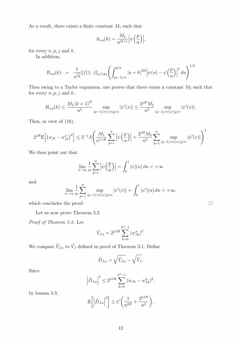
Applying Formula 20 in [7],

Var(VJ) = 2B2−J−4JH

∫ |ψ(λ)|4|λ|2+4H

dλ

+2A22−J−4H

2J−1∑

l=−2J+1

(∫eilλ|ψ(λ)|2|λ|1+2H

dλ

)2

+2−2J−4JHB

2J−1∑

l=−2J+1

∫e2ilλ|ψ(λ)|4|λ|2+4H

dλ

= (I) + (II) + (III).

with A = 4a2∫

C|z|2 ν(dz) + b2 and B = 4a2

∫C|z|2 ν(dz). For the second term, we first

point out that ψ is continuously differentiable. Then using that lim|λ|→+∞ ψ(λ) = 0 and

ψ(0) = 0, partial integration yields that

∫eilλ|ψ(λ)|2|λ|1+2H

dλ =−1

il

∫eilλ d

dλ

(|ψ(λ)|2|λ|1+2H

)dλ.

Hence we can conclude that∣∣∣∣∣

∫eilλ|ψ(λ)|2|λ|1+2H

dλ

∣∣∣∣∣

2

6c

1 + l2,

for c a given finite positive constant and every λ ∈ R.

Let us recall that∫tψ(t)dt = 0, so that ψ(ξ) = O

(|ξ|2)

as ξ → 0. The third term ishandled the same way (owing two integrations by parts), which enables us to concludethat ∣∣∣∣∣

∫e2ilλ|ψ(λ)|4|λ|2+4H

dλ

∣∣∣∣∣ 6c

1 + l2, ∀l ∈ R.

Finally, we obtain that the order of the variance is given by the terms (I) and (II) so

VarVJ ∼ DH2−J−4JH ,

with

0 < DH = 2B

∫

R

|ψ(λ)|4|λ|2+4H

dλ+ 2A2

∞∑

l=−∞

(∫

R

eilλ|ψ(λ)|2|λ|1+2H

dλ

)2

= 2B

∫

R

|ψ(λ)|4|λ|2+4H

dλ+ 4A2

∞∑

l=1

(∫

R

cos (lλ)|ψ(λ)|2|λ|1+2H

dλ

)2

+ 2C4H < +∞

9

This implies after renormalization that

VarVJ+∞∼ DH2−J =>

+∞∑

J=1

VarVJ < +∞.

The Borel Cantelli lemma yields that

22JHVJJ→+∞−→ E(w2

00) 6= 0, a.s .

Finally we obtain the result

−1

2Jlog2(VJ)

J→+∞−→ H a.s .

3.2 Discretized version

Suppose we observe XH(l/N), l = 0 . . . N . The size of data is then N + 1 and thewavelet type coefficients wjk can not be evaluated. However, the discretized coefficients

wnjk =

1

2j/2n

n∑

p=1

XH

(p+ nk

2jn

)ψ(p

n), k = 0 . . . 2j − 1, j = 0 . . . J

can be computed taking n = n(j) such that 2−jN/n(j) ∈ N. Also, we replace wJk by wnJk

in (14) and then obtain a new estimator which can be computed. Next theorem givesits consistency. Note that the parameter of discretization n depends on j and that theminimal size of data we need is 2Jn(J) + 1. In the following, we then take N = 2Jn(J).

Theorem 3.2. Consider the Hurst exponent estimator of a RHFLM defined as

HJ =−1

2Jlog2

2J−1∑

k=0

(wnJk)

2

(15)

with n = n(J) = 2J and with size of data N+1 = 22J +1. Provided ψ has r ≥ 1 vanishingmoment, the following asymptotics holds

HJJ→+∞−→ H, a.s.

Before proving Theorem 3.2, we state a result about the difference wjk−wnjk in norm L2.

In particular, a rate of convergence of wnjk in norm L2 is given for each fixed j and k.

Moreover, from the result established, we will deduced a comparison between the estima-tors defined by (14) and (15) and how to link n and J in (15), and then the size of dataN + 1 and J , in order to obtain the asymptotic behaviour of (15).

Lemma 3.3. There exists a constant C > 0 such that for every (j, k, n), j ∈ N\{0},k = 0 . . . 2j − 1, n ∈ N\{0},

22jHE[(wjk − wn

jk

)2] ≤ C

(1

2jn2H+

22jH

2jn2

).

10

Proof of Lemma 3.3. Let fH(x, ξ) =e−ixξ − 1

|ξ|H+1/2and

hn(k, ξ) =

∫ 1

0

fH(u+ k, ξ)ψ(u) du− 1

n

n∑

p=1

fH

(pn

+ k, ξ)ψ(pn

).

Since

wjk − wnjk = 2−j/2

∫

R

hn

(k, 2−jξ

)L(dξ),

in view of (5),

E

[(wjk − wn

jk

)2]= 2−jA

∫

R

∣∣hn

(k, 2−jξ

)∣∣2 dξ

= 2−j−2jHA

∫

R

|hn(k, λ)|2 dξ.

Then let us write

hn(k, λ) =n∑

p=1

hn,p(k, λ),

with

hn,p(k, λ) =

∫ p/n

(p−1)/n

(fH(u+ k, λ)ψ(u) − fH

(pn

+ k, λ)ψ(pn

))du.

By the Minkowski inequality,

22jHE[(wjk − wn

jk

)2] ≤ 2−jA

(n∑

p=1

‖hn,p(k, ·)‖L2(R)

)2

. (16)

Moreover, the Cauchy-Schwarz inequality implies that

|hn,p(k, λ)|2 ≤ 1

n

∫ p/n

(p−1)/n

∣∣∣fH(u+ k, λ)ψ(u) − fH

(pn

+ k, λ)ψ(pn

)∣∣∣2

du.

Therefore, applying the Minkowski inequality, we obtain:

‖hn,p(k, ·)‖L2(R) ≤ An,p(k) +Bn,p(k)

where

An,p(k) =1√n

(∫ p/n

(p−1)/n

∥∥∥f(u+ k, ·) − f(pn

+ k, ·)∥∥∥

2

L2(R)ψ2(pn

)du

)1/2

and

Bn,p(k) =1√n

(∫ p/n

(p−1)/n

‖f(u+ k, ·)‖2L2(R)

∣∣∣ψ(u) − ψ(pn

)∣∣∣2

du

)1/2

.

Let us first point out that

∥∥f(u+ k, ·) − f(

pn

+ k, ·)∥∥2

L2(R)=

∥∥∥f(u− p

n, ·)∥∥∥

2

L2(R)

=∣∣∣u− p

n

∣∣∣2H

‖f(1, ·)‖2L2(R).

11

As a result, there exists a finite constant M1 such that

An,p(k) =M1

nH+1

∣∣∣ψ(pn

)∣∣∣,

for every n, p, j and k.In addition,

Bn,p(k) =1√n‖f(1, ·)‖L2(R)

(∫ p/n

(p−1)/n

|u+ k|2H∣∣∣ψ(u) − ψ

(pn

)∣∣∣2

du

)1/2

Then owing to a Taylor expansion, one proves that there exists a constant M2 such thatfor every n, p, j and k,

Bn,p(k) ≤M2 (k + 1)H

n2sup

(p−1)/n≤x≤p/n

|ψ′(x)| ≤ 2jHM2

n2sup

(p−1)/n≤x≤p/n

|ψ′(x)|.

Then, in view of (16),

2jHE

[(wjk − wn

jk

)2] ≤ 2−jA

(M1

n1+H

n∑

p=1

∣∣∣ψ(pn

)∣∣∣+2jHM2

n2

n∑

p=1

sup(p−1)/n≤x≤p/n

|ψ′(x)|)2

.

We then point out that

limn→∞

1

n

n∑

p=1

∣∣∣ψ(pn

)∣∣∣ =

∫ 1

0

|ψ|(u) du < +∞

and

limn→∞

1

n

n∑

p=1

sup(p−1)/n≤x≤p/n

|ψ′(x)| =

∫ 1

0

|ψ′|(u) du < +∞,

which concludes the proof.

Let us now prove Theorem 3.2.

Proof of Theorem 3.2. Let

VJ,n = 22JH

2J−1∑

k=0

(wnJk)

2.

We compare VJ,n to VJ defined in proof of Theorem 3.1. Define

DJ,n =

√VJ,n −

√VJ .

Since∣∣∣DJ,n

∣∣∣2

≤ 22JH

2J−1∑

k=0

(wJk − wnJk)

2,

by lemma 3.3,

E

[∣∣∣DJ,n

∣∣∣2]≤ C

(1

n2H+

22JH

n2

),

12

where C is a finite constant. Taking n = n(J) = 2J , the Borel Cantelli lemma yields thatas J → +∞,

DJ,2J → 0, a.s.

Recall that , as J → +∞,VJ → E

(w2

00

)a.s.

Then,VJ,2J → E

(w2

00

)a.s,

which leads to the convergence of HJ defined by (15).

4 Regression framework

Suppose we observe noisy data from a RHFLM XH

YH

(l

N

)= XH

(l

N

)+ σNεl, l = 0, . . . , N, (17)

where εl are an i.i.d sample of Gaussian random variables N (0, 1) and σN is the noise

level. We point out that σN = O(N− 1

2 ). This framework is the usual regression settingwell studied in statistics, which models natural observations of a phenomenom, observedat discrete times.

The discretized coefficients wnjk of XH can not be observed. However, the discretized

coefficients of YH

dnjk =

1

2j/2n

n∑

p=1

YH

(p+ nk

2jn

)ψ(p

n), k = 0 . . . 2j − 1, j = 0 . . . J,

can be computed, taking N = 22J and n = n(j) such that 2−jN/n(j) ∈ N as in Section 3.

Theorem 4.1. Consider the estimator of the Hurst coefficient of a RHFLM defined as

HJ =−1

2Jlog2

2J−1∑

k=0

(dnJk)

2

(18)

with n = n(J) = 2J and N = 22J . Provided ψ has at least r ≥ 1 vanishing moments, thefollowing asymptotics holds

HJJ→+∞−→ H, a.s.

Proof. We proceed as in the proof of Theorem 3.2. Let us recall that

VJ,n = 22JH

2J−1∑

k=0

(wnJk)

2

and define

WJ,n = 22JH

2J−1∑

k=0

(dnJk)

2.

13

Then,

E

(∣∣∣∣√WJ,n −

√VJ,n

∣∣∣∣2)

≤ 22JH

2J−1∑

k=0

E[(dn

Jk − wnJk)

2].

By definition of YH ,

dnJk − wn

Jk =1

2J/2nσN

n∑

p=1

ψ(pn

)εp+nk ∼ N

(0,

σ2N

2Jn2

n∑

p=1

ψ2(pn

)).

Hence,

E

(∣∣∣∣√WJ,n −

√VJ,n

∣∣∣∣2)

≤ 22JHσ2N

n2

n∑

p=1

ψ2(pn

).

Since limn→+∞1n

∑np=1 ψ

2(

pn

)=∫

Rψ2(u)du = 1, there exists a constant C ∈ (0,+∞)

such that for every J and n,

E

(∣∣∣∣√WJ,n −

√VJ,n

∣∣∣∣2)

≤ 22JHCσ2N

n.

Also, taking n = n(J) = 2J , the Borel Cantelli Lemma yields that

√WJ,2J −

√VJ,2J

J→+∞−→ 0 a.s.,

as soon as σN = O(N−1/2) with N = 22J . Then, since (see proof of Theorem 3.2),

VJ,2J

J→+∞−→ E(w2

00

)a.s.,

we finally obtain that

HJ = − 1

2Jlog2

(2−2JHWJ,2J

)J→+∞−→ H a.s.,

as soon as σN = O(N−1/2) with N = 2Jn(J) = 22J .

As a result, we obtain consistency of the estimators in the practical case where theRHFLM is observed at discrete times. This result can be used to build an estimatorof the Hurst exponent when studying the outcome of an experiment though to behavelike a RHFLM. Once this parameter is estimated it becomes possible to try to modelthe data by a realization of a RHFLM. Hence, it should be of interest to construct atest based on the estimator of the Hurst exponent. So the asymptotic distribution ofthe estimator is needed. However, such a result is very difficult to obtain. On the onehand, the nature of the observations prevents the use of Central Limit type theorems. Onthe other hand, evaluating the distance between the distribution of the coefficients of aRHFLM and a Gaussian distribution is also far beyond the scope of this paper due sincethe calculations can only be handled using (3), preventing the use of weak dependencytheorems. Nevertheless a consistency result is a first step in a modeling attempt withRHFLM.

14

5 Numerical study

In this section, consider the issue of estimating the Hurst exponent of a RHFLM observedwith a Gaussian white noise. In the simulations we present in Figure 1 and 2 simulateddata in straight lines, obtained using the procedure described in [23], together with thenoisy paths in dotted lines.

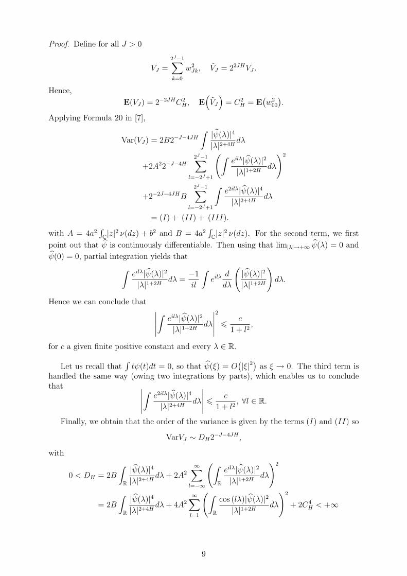
First we aim at studying the rate of convergence of the wavelet type estimator. Theestimator of the Hurst exponent is constructed using rescaled Daubechies wavelet Db(4)with r = 4 vanishing moments. We construct the estimator of the Hurst exponent for thetwo previous RHFLMs with the two different values of the Hurst exponent H = .4 andH = .7. The data are dyadic N = 22J and we increase the data from J = 2 to J = 7.For the noisy data, we perform 30 replications of the estimation procedure and plot theboxplots for the absolute error for different values of J in Figure 3 and Figure 4. In bothcases, we can see that the convergence is achieved with N > 28 observations. Such studyhighlights consistency of the estimate. But, due to the relative slowness of the rate ofconvergence together with the lack of an asymptotic distribution law, it is difficult toestimate the efficiency of such an estimation procedure for real data.

0 0.1 0.2 0.3 0.4 0.5 0.6 0.7 0.8 0.9 1−2

−1

0

1

2

3

4

5

6

7

8

Figure 1: Raw and Noisy Data with H = .4

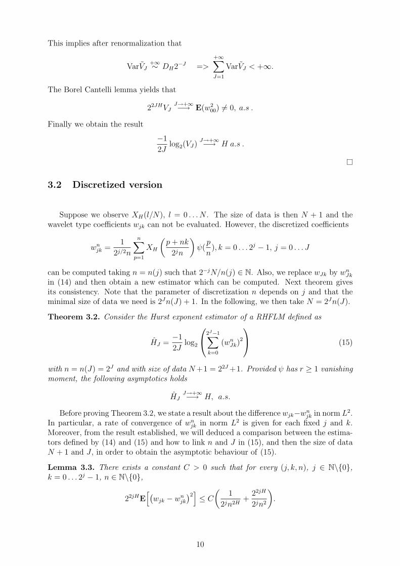
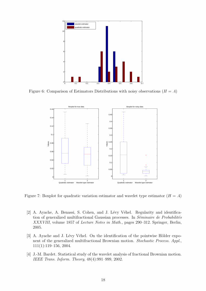
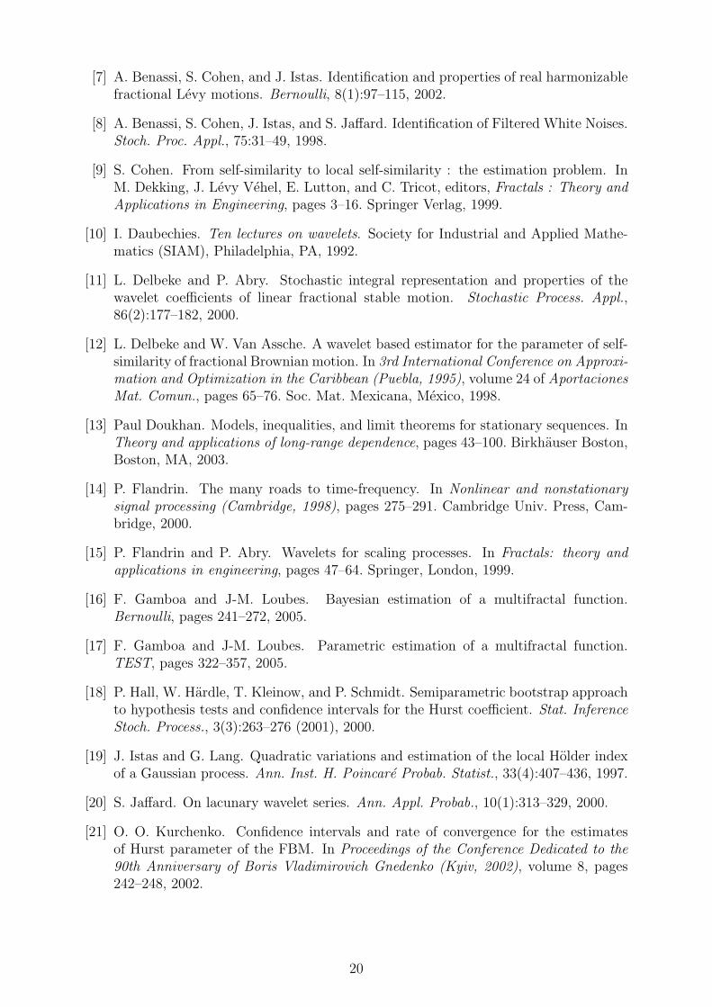
However we can compare the efficiency of our estimator with the estimator given in[7]. We compute this estimator and the estimator constructed in Section 3, when H = .4for two cases, whether or not the RHFLM is observed with a Gaussian white noise. Wetake N = 210 observations and consider 30 replications. We plot the distribution of bothestimators, first the distribution of the wavelet type estimator and then the distributionof the quadratic variation based estimator. We observe in Figure 5 that without noise, thetwo estimators give the same kind of results. But, as expected, in a noisy setup, in Figure6, the estimator based on quadratic variation does not concentrate around the true valueof the Hurst parameter. This result is also highlighted by the boxplot of the absolute

15

0 0.2 0.4 0.6 0.8 1−1.5

−1

−0.5

0

0.5

1

1.5

2

Figure 2: Raw and Noisy Data with H = .7

2 3 4 5 6 7

0

0.1

0.2

0.3

0.4

0.5

0.6

0.7

Val

ues

J, N=22J

Figure 3: Absolute Estimation Error for noisy data with H = .4

error of the two estimators, in Figure 7. The absolute error of estimation is important inthe noisy setup for the quadratic type estimator.

Finally, we study the relative influence in the choice of the mother wavelet by com-puting the distribution of the absolute estimation error of the estimation of H = .4 withnoisy data for 30 simulations and two different sets of coefficients, obtained for a rescaled

16

2 3 4 5 6 7

0

0.05

0.1

0.15

0.2

0.25

0.3

0.35

0.4

0.45

0.5

Val

ues

J, N=22J

Figure 4: Absolute Estimation Error for noisy data with H = .7

0.3 0.32 0.34 0.36 0.38 0.4 0.42 0.44 0.46 0.480

2

4

6

8

10

12

14

wavelet estimatorquadratic estimator

Figure 5: Comparison of Estimators Distributions with true observations (H = .4)

Daubechies wavelet with r = 4 and for r = 2. We can see in Figures 8 and Figures 9 thatthe distribution are similar. So as expected and as usual in estimation with wavelet typeestimators, the choice of the wavelet does not play a particular role in the estimation aslong as the initial assumptions are met.

References

[1] P. Abry, P. Flandrin, M. S. Taqqu, and D. Veitch. Self-similarity and long-rangedependence through the wavelet lens. In Theory and applications of long-range de-pendence, pages 527–556. Birkhauser Boston, Boston, MA, 2003.

17

0 0.1 0.2 0.3 0.4 0.5 0.6 0.70

2

4

6

8

10

12

wavelet estimator

quadratic estimator

Figure 6: Comparison of Estimators Distributions with noisy observations (H = .4)

1 2

0

0.02

0.04

0.06

0.08

0.1

0.12

0.14

0.16

Val

ues

Quadratic estimator Wavelet type estimator

Boxplot for true data

1 2

0

0.05

0.1

0.15

0.2

0.25

0.3

0.35

0.4

0.45

Val

ues

Quadratic estimator Wavelet type estimator

Boxplot for noisy data

Figure 7: Boxplot for quadratic variation estimator and wavelet type estimator (H = .4)

[2] A. Ayache, A. Benassi, S. Cohen, and J. Levy Vehel. Regularity and identifica-tion of generalized multifractional Gaussian processes. In Seminaire de ProbabilitesXXXVIII, volume 1857 of Lecture Notes in Math., pages 290–312. Springer, Berlin,2005.

[3] A. Ayache and J. Levy Vehel. On the identification of the pointwise Holder expo-nent of the generalized multifractional Brownian motion. Stochastic Process. Appl.,111(1):119–156, 2004.

[4] J.-M. Bardet. Statistical study of the wavelet analysis of fractional Brownian motion.IEEE Trans. Inform. Theory, 48(4):991–999, 2002.

18

0 0.02 0.04 0.06 0.08 0.1 0.12 0.14 0.16 0.180

2

4

6

8

10

12

Figure 8: Distribution of Absolute Error for noisy data with H = .4 using Db(4)

0 0.02 0.04 0.06 0.08 0.1 0.12 0.14 0.16 0.18 0.20

2

4

6

8

10

12

Figure 9: Distribution of Absolute Error for noisy data with H = .4 using Db(2)

[5] A. Benassi, P. Bertrand, S. Cohen, and J. Istas. Identification of the Hurst index ofa step fractional Brownian motion. Stat. Inference Stoch. Process., 3(1-2):101–111,2000. 19th “Rencontres Franco-Belges de Statisticiens” (Marseille, 1998).

[6] A. Benassi, S. Cohen, and J. Istas. Identifying the multifractional function of aGaussian process. Statistic and Probability Letters, 39:337–345, 1998.

19

[7] A. Benassi, S. Cohen, and J. Istas. Identification and properties of real harmonizablefractional Levy motions. Bernoulli, 8(1):97–115, 2002.

[8] A. Benassi, S. Cohen, J. Istas, and S. Jaffard. Identification of Filtered White Noises.Stoch. Proc. Appl., 75:31–49, 1998.

[9] S. Cohen. From self-similarity to local self-similarity : the estimation problem. InM. Dekking, J. Levy Vehel, E. Lutton, and C. Tricot, editors, Fractals : Theory andApplications in Engineering, pages 3–16. Springer Verlag, 1999.

[10] I. Daubechies. Ten lectures on wavelets. Society for Industrial and Applied Mathe-matics (SIAM), Philadelphia, PA, 1992.

[11] L. Delbeke and P. Abry. Stochastic integral representation and properties of thewavelet coefficients of linear fractional stable motion. Stochastic Process. Appl.,86(2):177–182, 2000.

[12] L. Delbeke and W. Van Assche. A wavelet based estimator for the parameter of self-similarity of fractional Brownian motion. In 3rd International Conference on Approxi-mation and Optimization in the Caribbean (Puebla, 1995), volume 24 of AportacionesMat. Comun., pages 65–76. Soc. Mat. Mexicana, Mexico, 1998.

[13] Paul Doukhan. Models, inequalities, and limit theorems for stationary sequences. InTheory and applications of long-range dependence, pages 43–100. Birkhauser Boston,Boston, MA, 2003.

[14] P. Flandrin. The many roads to time-frequency. In Nonlinear and nonstationarysignal processing (Cambridge, 1998), pages 275–291. Cambridge Univ. Press, Cam-bridge, 2000.

[15] P. Flandrin and P. Abry. Wavelets for scaling processes. In Fractals: theory andapplications in engineering, pages 47–64. Springer, London, 1999.

[16] F. Gamboa and J-M. Loubes. Bayesian estimation of a multifractal function.Bernoulli, pages 241–272, 2005.

[17] F. Gamboa and J-M. Loubes. Parametric estimation of a multifractal function.TEST, pages 322–357, 2005.

[18] P. Hall, W. Hardle, T. Kleinow, and P. Schmidt. Semiparametric bootstrap approachto hypothesis tests and confidence intervals for the Hurst coefficient. Stat. InferenceStoch. Process., 3(3):263–276 (2001), 2000.

[19] J. Istas and G. Lang. Quadratic variations and estimation of the local Holder indexof a Gaussian process. Ann. Inst. H. Poincare Probab. Statist., 33(4):407–436, 1997.

[20] S. Jaffard. On lacunary wavelet series. Ann. Appl. Probab., 10(1):313–329, 2000.

[21] O. O. Kurchenko. Confidence intervals and rate of convergence for the estimatesof Hurst parameter of the FBM. In Proceedings of the Conference Dedicated to the90th Anniversary of Boris Vladimirovich Gnedenko (Kyiv, 2002), volume 8, pages242–248, 2002.

20

[22] C. Lacaux. Real harmonizable multifractional Levy motions. Ann. Inst. H. PoincareProbab. Statist., 40(3):259–277, 2004.

[23] C. Lacaux. Series representation and simulation of multifractional Levy motions.Adv. Appl. Probab., 36(1):171–197, 2004.

[24] S. Mallat. A wavelet tour of signal processing. Academic Press Inc., San Diego, CA,1998.

[25] B. Mandelbrot and J. Van Ness. Fractional Brownian motion, fractionnal noises andapplications. Siam Review, 10:422–437, 1968.

[26] C. Morales and E. Kolaczyk. Analysis of wavelet-based estimators of the Hurstparameter. Preprint 2004.

[27] V. Pipiras, M. S. Taqqu, and P. Abry. Asymptotic normality for wavelet-basedestimators of fractional stable motion. Preprint 2004.

[28] G. Samorodnitsky and M. S. Taqqu. Stable non-Gaussian random processes. Stochas-tic Modeling. Chapman & Hall, New York, 1994. Stochastic models with infinitevariance.

[29] S. Stoev, P. Pipiras, and M. S. Taqqu. Estimation of the self-similarity parameter inlinear fractional stable motion. Signal Processing, 82:1873–1901, 2002.

Celine Lacaux.Address: Ecole des Mines de Nancy (INPL), Parc de Saurupt, CS 14234, 54042 Nancy cedex France.Institut Elie Cartan, Universite Henri Poincare, BP 239, F-54506 Vandoeuvre-Les-Nancy cedex, France.E-mail: lacaux@iecn.u-nancy.frWeb-site: http://www.lsp.ups-tlse.fr/Fp/Lacaux

Jean-Michel Loubes.

Address: UMR 8628 CNRS, Batiment 9, Departement de Mathematiques, Equipe de Probabilites et

Statistique, Universite de Montpellier II, Place E. Bataillon, 34000 Montpellier, Cedex, France.

E-mail: mailto:Jean-Michel.Loubes@math.univ-montp2.fr

Web-site: http://www.math.univ-montp2.fr/~loubes/

21