J GeodDOI 10.1007/s00190-011-0519-2

ORIGINAL ARTICLE

Numerical computation of spherical harmonics of arbitrarydegree and order by extending exponent of floating point numbers

Toshio Fukushima

Received: 25 May 2011 / Accepted: 1 October 2011© Springer-Verlag 2011

Abstract By extending the exponent of floating point num-bers with an additional integer as the power index of a largeradix, we compute fully normalized associated Legendrefunctions (ALF) by recursion without underflow problem.The new method enables us to evaluate ALFs of extremelyhigh degree as 232 = 4,294,967,296, which corresponds toaround 1 cm resolution on the Earth’s surface. By limitingthe application of exponent extension to a few working vari-ables in the recursion, choosing a suitable large power of 2as the radix, and embedding the contents of the basic arith-metic procedure of floating point numbers with the exponentextension directly in the program computing the recurrenceformulas, we achieve the evaluation of ALFs in the double-precision environment at the cost of around 10% increase incomputational time per single ALF. This formulation real-izes meaningful execution of the spherical harmonic synthe-sis and/or analysis of arbitrary degree and order.

Keywords Associated Legendre functions · Exponentextension · Floating point number · Spherical harmonics ·Underflow problem

1 Introduction

The gravity field of a celestial object like the Earth is usuallyexpressed as the spherical harmonic expansion (Kaula 2000).So the gravity anomaly, the geoid undulation, the deflectionof the vertical, and the variance/covariance of physical geo-detic observations can be also expressed in terms of truncatedspherical harmonic expansion.

T. Fukushima (B)National Astronomical Observatory, Ohsawa, Mitaka,Tokyo 181-8588, Japane-mail: Toshio.Fukushima@nao.ac.jp

For example, the geopotential is frequently written in theform of truncated Fourier series with respect to the longitudeas

V (r, φ, λ) = G ME

r

(c0 +

M∑m=1

(cm cos mλ + sm sin mλ)

),

(1)

where

c0 ≡ 1 +N∑

n=2

(ae

r

)nCn0 Pn(sin φ), (2)

cm ≡N∑

n=max(2,m)

(ae

r

)nCnm P

mn (sin φ), (3)

sm ≡N∑

n=max(2,m)

(ae

r

)nSnm P

mn (sin φ), (4)

are the Fourier coefficients, sometimes called as “lumpedcoefficients”.

Here r, φ, and λ are the geocentric distance, the geocen-tric latitude, and the longitude of an external point, GM E isthe geocentric gravitational constant, N and M are the max-imum degree and order of the truncated expansion, ae is theequatorial radius of the Earth, Cnm and Snm are the fullynormalized Stokes coefficients of the Earth of degree n and

order m, Pn(t) ≡ P0n (t) is the fully normalized Legendre

polynomial (LP) of the first kind of degree n and argument tas explained in Chapter 18 of Olver et al. (2010), and P

mn (t)

is the fully normalized associated Legendre function (ALF)of the first kind of degree n, order m, and argument t asdescribed in Chapter 14 of Olver et al. (2010).

Once the lumped coefficients are obtained, the geopoten-tial is efficiently computed by the Fast Fourier Transform(FFT) (Cooley and Tukey 1965). Thus the problem reduces

123

T. Fukushima

Table 1 Special numbers in IEEE754-2008 floating point arithmetic.Shown are approximate magnitudes of the machine epsilon, ε, and themaximum and minimum representable numbers, ω and δ, in the single,double, and quadruple precision environments in the IEEE754-2008standard (IEEE 2008), respectively

Precision ε ω δ

Single 1.19 × 10−7 3.40 × 1038 1.18 × 10−38

Double 1.11 × 10−16 1.80 × 10308 2.23 × 10−308

Quadruple 9.63 × 10−35 1.19 × 104932 6.48 × 10−4966

A number is expressed in computers as Infinity if its absolute valueexceeds ω. This phenomenon is called an overflow. Meanwhile, a non-zero number is practically treated as 0 when its absolute value is lessthan δ. This is named an underflow

to the simultaneous computation of LPs and ALFs of variousorder and degree for the same argument.

From a pure mathematical point of view, the definition1 ofLPs and ALFs is well established (Kelogg 1929; Heiskanenand Moritz 1967). In practical computation, however, we facedifficulties in computing ALFs independently on the styleof normalization when N and/or M become large, say morethan a few thousands (Wenzel 1998). This is due to the narrowdynamic range of the real numbers representable at currentcomputers (Wittwer et al. 2008).

A non-integer real number is approximately expressed bya floating point number in almost all computer architecturesand in popular computer languages such as C or Fortran(Goldberg 1991). In the IEEE754-2008 (IEEE 2008), thecurrent industry standard specifying the floating point arith-metic, the expression of a real number becomes inappropriateif its absolute value is (1) larger than the maximum represent-able number, ω, or (2) smaller than the minimum represent-able number, δ, except a very rare case when the numberis exactly equal to zero. These special numbers are listedin Table 1 together with the so-called machine epsilon, ε,expressing the smallest meaningful number. More rigorouslyspeaking, (1) ε is the least number satisfying the condition,1 + ε �= 1, (2) ω is the least number such that the operation(1+ ε)ω returns Infinity, and (3) η is the largest numberleading to the relation, (1 − ε)η = 0.

This practical limitation hinders meaningful computationof ALFs without tricks (Deprit 1979; Gleason 1985; Holmesand Featherstone 2002; Casotto and Fantino 2007; Fantinoand Casotto 2009). Usually the ALFs are computed by three-term recursions starting from the sectorial and semi-secto-rial terms, P

mm (sin φ) and P

mm+1(sin φ). Since P

mn (sin φ) ∝

cosm φ, these seed values suffer underflow if cos φ is suf-ficiently small and/or the degree m is sufficiently large. In

1 There is an ambiguity of the factor (−1)m in Pmn (t) in the literature

(Wolfram 2003; Olver et al. 2010). This is due to the difference in theviewpoint to regard ALFs as the derivatives of LPs with respect to thelatitude φ or the co-latitude θ ≡ π/2 − φ.

that case, all the ALFs obtained by recursion become zeroeven if the recursion should have amplified the seed values.Namely, the underflow of the two starting values propagate soas to make the subsequent computation of ALFs meaningless.This is the underflow problem of fully and quasi-normalizedALFs.

The underflow problem of normalized ALFs can beresolved by separating the factor cosm φ. An example isthe replacement of ALFs by the Helmholtz polynomialsdefined as Hnm(sin φ) ≡ P

mn (sin φ)/ cosm φ. Refer to Sec-

tion 5 of Fantino and Casotto (2009). Nevertheless, this time,an overflow occurs in the recursion to compute the Helm-holtz polynomials. This also deteriorates the resulting spher-ical harmonic expansions. In the end, within the standardIEEE754 arithmetic, we can not get rid of underflow or over-flow problems in the recursion unless we use some device.

In fact, a latest geopotential model EGM2008 (Pavliset al. 2008) was successfully prepared in the double-precisionenvironment by means of the fully normalized ALFs (Heiska-nen and Moritz 1967) and the global scaling by 10250, asuitable huge constant of the order of ω5/6 (Wenzel 1998),despite its maximum degree and order are as large as N =2,190 and M = 2,159, respectively. However, these tech-niques will be no longer effective in treating spherical har-monics of higher degree, say when N and/or M is greaterthan 2,700 in the double-precision environment.

Of course, we can extend the limit somewhat by com-puting them in the quadruple precision. For example, thefull normalization in the quadruple precision computationenables the evaluation of ALFs of degree 10,800 (Jekeli et al.2007). Nevertheless, the shift of computing precision fromthe double to quadruple precision environment requires aquite large computational labor, say 40–80 times that of thedouble-precision computation, in addition to doubling thenecessary memory.

Also, the quadruple precision computation cannot resolvethe problem essentially. Sooner or later, we face the samedifficulties when we increase N and/or M . Indeed, whenM = 21,600, the quadruple precision computation of fullynormalized ALFs without a suitable pre-scaling suffers fromunderflows if φ > 53◦50′.

An ultimate solution to this overflow/underflow problemwould be to use an extended-range arithmetic (Smith et al.1981) or, more generally, an arbitrary-precision arithmetic(Brent 1978; Wolfram 2003). The latter formulation is suf-ficiently powerful but known to run quite slow. On the otherhand, a recent research revealed that an application of theextended-range arithmetic software package developed byLozier and Smith (1981) to the spherical harmonic synthesiscould effectively compute the harmonics of extremely highdegree, say 3,000 and much higher (Wittwer et al. 2008).However, this was achieved at the cost of around 50 timesincrease in the computational time. On the other hand, the

123

Numerical computation of spherical harmonics

evaluation of ALFs themselves is realized at the computa-tional cost of around a factor 2 increase (Smith et al. 1981)as will be confirmed later in Sect. 3.4.

In conducting the extended-range arithmetic, only a part ofquantities are to be regarded as the numbers with exponentextension. Also, only a few types of mathematical opera-tion are to be conducted with the extended-range arithme-tic. Indeed, a suitable choice of the radix greatly simplifiesthese mathematical operations. Further, we expect that thedirect embedding of these basic routines into the programcalling them significantly accelerates the computation usingthe extended-range arithmetic. In this article, we report thata limited usage of thus-modified extended-range arithmeticenables the meaningful computation of geopotential of arbi-trary degree and order in the double-precision environmentwith a negligibly small increase in the computational time.

2 Method

2.1 Extension of exponent

Modifying the idea of extended-range arithmetic (Smith et al.1981) a little, we represent a non-zero arbitrary real number,X , by a pair of an IEEE754 floating point number, x , and asigned integer, iX . More specifically speaking, we choose acertain large power of 2 as the radix, B, and regard x andiX as the significand and the exponent with respect to it.Namely, we express X as X = x BiX . The major differencefrom Smith et al. (1981) is the choice of the radix as will beexplained in Appendix A.6.

Let us call such a pair, (x, iX ), an extended exponent num-ber and abbreviate it to X-number. Meanwhile, we denotea non-zero ordinary floating point number by F-number inshort. The detailed definition of X- and F-numbers is givenin Appendix A.1.

2.2 Mathematical operations of X-numbers

The extended-range arithmetic is applicable to ALFs of allkind of normalization: no normalization, quasi-normaliza-tion (Tscherning and Poder 1982; Tscherning et al. 1983), orfull-normalization (Heiskanen and Moritz 1967). Therefore,we select one of them, the full-normalization, for simplicity.

In the framework of full-normalization, it is easy to see thatX-numbers in the spherical harmonic expansions are limitedto a few working variables to compute ALFs by recursion.In fact, the fully normalized ALFs themselves can be storedas F-numbers (Heiskanen and Moritz 1967). Also, the com-putation of fully normalized LPs is well executed withoutusing X-numbers at all (Jekeli et al. 2007). Further, the fullynormalized Stokes coefficients are F-numbers (Pavlis et al.2008). On the other hand, the derivatives of ALFs can be com-

puted from ALFs themselves (Bosch 2000). Meanwhile, theintegral of ALFs can be computed without using X-numbersif ALFs are obtained as F-numbers. See the discussion inAppendix B.

In conclusion, only two types of mathematical operationare to be conducted using X-numbers: a two-term linear sumof X-numbers with F-number coefficients, Z = f X + gY ,and, as its degenerate form, the F-number multiplication ofan X-number, Y = f X . Here X, Y , and Z are X-numbersand f and g are F-numbers.

2.3 Recursion formulas of ALF

The X-number operations discussed in the above appearin the recursion formulas to compute ALFs. An example ofthe first type operation is the fixed-order, increasing-degree,consecutive three-term recurrence formula:

pnm = (anm sin φ) pn−1,m

+ (−bnm) pn−2,m, (n ≥ m + 2) (5)

where we abbreviate Pmn (sin φ) to pnm and

anm ≡√

(2n + 1)(2n − 1)

(n + m)(n − m), (6)

bnm ≡ anm

an,m−1=

√(2n + 1)(n + m − 1)(n − m − 1)

(2n − 3)(n + m)(n − m), (7)

are numerical coefficients depending on n and m only. Usu-ally, these latitude-independent quantities are pre-computed,stored, and re-used.

A specimen of the second type operation is the recurrenceformula to obtain the sectorial ALF,

pmm = (dm cos φ) pm−1,m−1, (m ≥ 2) (8)

where

dm ≡√

2m + 1

2m. (9)

is a numerical coefficient depending on m only. The startingvalue of this recursion is computed by definition as

p11 = √3 cos φ. (10)

Another example of the second type occurs in computing thesemi-sectorial ALFs, pm+1,m , as

pm+1,m = (am+1,m sin φ)pmm . (m ≥ 1) (11)

This is a degenerate form of Eq. (5). By means of X-num-ber operations, all these recursions can be conducted withoutunderflow problems even near the pole such that cos φ is assmall as εdouble ≈ 1.11 × 10−16, the machine epsilon of thedouble-precision environment.

123

T. Fukushima

2.4 Limitation of X-number usage

We emphasize that the computed values of pnm can be storedas F-numbers after their reference in the recursion formula isfinished. Therefore, the usage of X-numbers can be limitedto a few working variables needed in the recursions of ALF.For example, the above three-term recursion, Eq. (5), may beexecuted by a do-loop increasing n as

f := anm sin φ, g := −bnm, Z := f X + gY, pnm := Z ,

Y := X, X := Z , n := n + 1, (12)

starting from the initialization

n := m + 1, X := pm+1,m, Y := pmm . (13)

Here X, Y, Z , pm+1,m , and pmm are X-numbers while f, g,

anm, bnm , and pnm are F-numbers. Namely, in this specificexample, one needs only 3 X-numbers and 2 F-numbers asworking variables.

The operation := means (1) a simple substitution if theboth sides are the same type numbers, and (2) translationbetween F- and X-numbers otherwise. The details of the lat-ter operation are described in Appendix A.2. See also sampleprocedures given in Sect. 2.7 later.

2.5 Stability

Consider the effect of X-number usage on the issue of sta-bility in computing ALFs. In general, the introduction ofX-numbers simply means the practically unrestricted exten-sion of exponent of real numbers treated. The situationis similar to the case of precision change, like the shiftfrom the double to quadruple precision computations. Inthat case, the shift means a moderate extension of man-tissa and exponent of real numbers treated. Therefore, thenature of stability of a certain recurrence formula willnot change by the X-number usage. An essentially unsta-ble algorithm remains unstable. So do the stable formu-las.

Of course, there may be a chance that the stability condi-tion of an occasionally unstable mechanism is relaxed by theintroduction of X-number. For example, if the instabilitiesare caused only by intermediate underflow/overflows due tothe multiplication/division by tiny factors, there is a room toovercome them using X-numbers. However, this issue is anopen problem that is worthy of further investigation in future.

2.6 Implementation

Let us return to practical issues. We may design the pro-cedures to compute pnm in four ways: (1) that to return asingle pnm for the given pair of n and m, (2) that to returna one-dimensional array of pnm for the given m and for

a series of n in the range, n1 ≤ n ≤ n2, under the condi-tion m ≤ n1, (3) that to return a one-dimensional arrayof pnm for the given n and for a series of m in the range,m1 ≤ m ≤ m2, under the condition m2 ≤ n, and (4)that to return a two-dimensional array of pnm for n and min the range, m1 ≤ m ≤ m2 and n1 ≤ n ≤ n2, underthe condition m ≤ n. We call them the scalar, fixed-ordervector, fixed-degree vector, and matrix procedures, respec-tively.

The difference in these four ways is firstly the mem-ory requirement, secondly the computing speed, and thirdlythe complexity of programs. Depending on the purpose ofcomputation and the available computing resource, one maychoose one of them.

In fact, the scalar procedure requires only a few workingvariables such that the degree and order can be arbitrary high.See Table 5 later. It lists sample values of pn,n/2 with n as highas 232 = 4,294,967,296 prepared by the scalar procedure.Nevertheless, one must calculate the numerical coefficients,anm, bnm , and dm , at every call of the scalar procedure. This isin order to save the memory space. As a result, the computingspeed is fairly slow.

Meanwhile, the matrix procedure assumes that all thecoefficients are (1) provided externally, or (2) computedinternally at the first call of it and stored. Then, the averagecomputing speed is the fastest. The CPU time comparisonshown in Fig. 3 later was conducted by this matrix version.However, this is at the cost of requiring a large amount ofworking memory. For example, a few ten thousands becomesthe maximum degree and order feasible within the frame-work of 32-bit OS and 3 GB main memory capacity. Ofcourse, the cost of main memory is relatively low nowa-days. Also the usage of 64-bit OS ensures the access toa huge memory in principle. Therefore, one may choosethis option when a good computing environment is avail-able.

2.7 Sample programs

Taking the moderate way, we present here sample pro-grams based on the second way, the fixed-order vectorprocedures. They are all written in Fortran in the double-precision environment. Tables 2 and 3 list prototype For-tran subroutines to compute the sectorial and non-sectorialfully normalized ALFs by calling the basic Fortran sub-routine and/or function of X-numbers: x2f,xnorm, andxlsum2. These subprograms are explicitly given in Appen-dices A.2, A.3, and A.5, respectively. The overhead to callthese subprograms are relatively large as will be shownlater in Fig. 3. Therefore, in the actual implementation, wedirectly embed their contents into the programs as shown inAppendix C.

123

Numerical computation of spherical harmonics

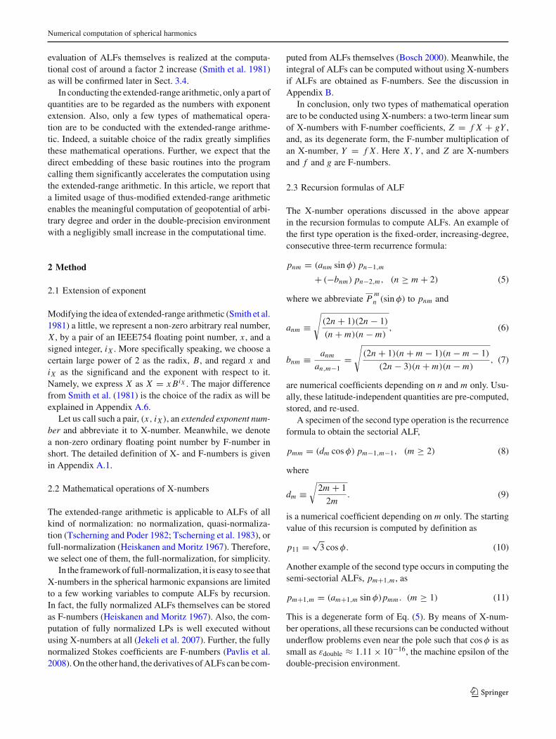
Table 2 Prototype Fortran subroutine to return a one-dimensional arrayof the fully normalized sectorial ALFs, pmm , in X-numbers. i.e. the pairsof the significand ps(m) and the exponent ips(m)

subroutine alfsp(u,mx,d,ps,ips)

integer mx,ips(*),m,ix

real*8 u,d(*),ps(*),ROOT3,x

parameter (ROOT3=1.7320508075688773d0)

x=ROOT3*u; ix=0; ps(1)=x; ips(1)=ix

do m=2,mx

x=(d(m)*u)*x; call xnorm(x,ix); ps(m)=x; ips(m)=ix

enddo

return; end

It calls the normalization subroutine of an X-number: xnorm, whichis given in Appendix A.3. We assume that the numerical constants,dm ≡ √

(2m + 1)/(2m), are externally provided. In the program, u ≡cos φ,mx is the maximum order M , and d(m) = dm . The digits of anumerical constant, ROOT3 ≡ √

3, are given more than enough for thepurpose to avoid unnecessary round-off errors

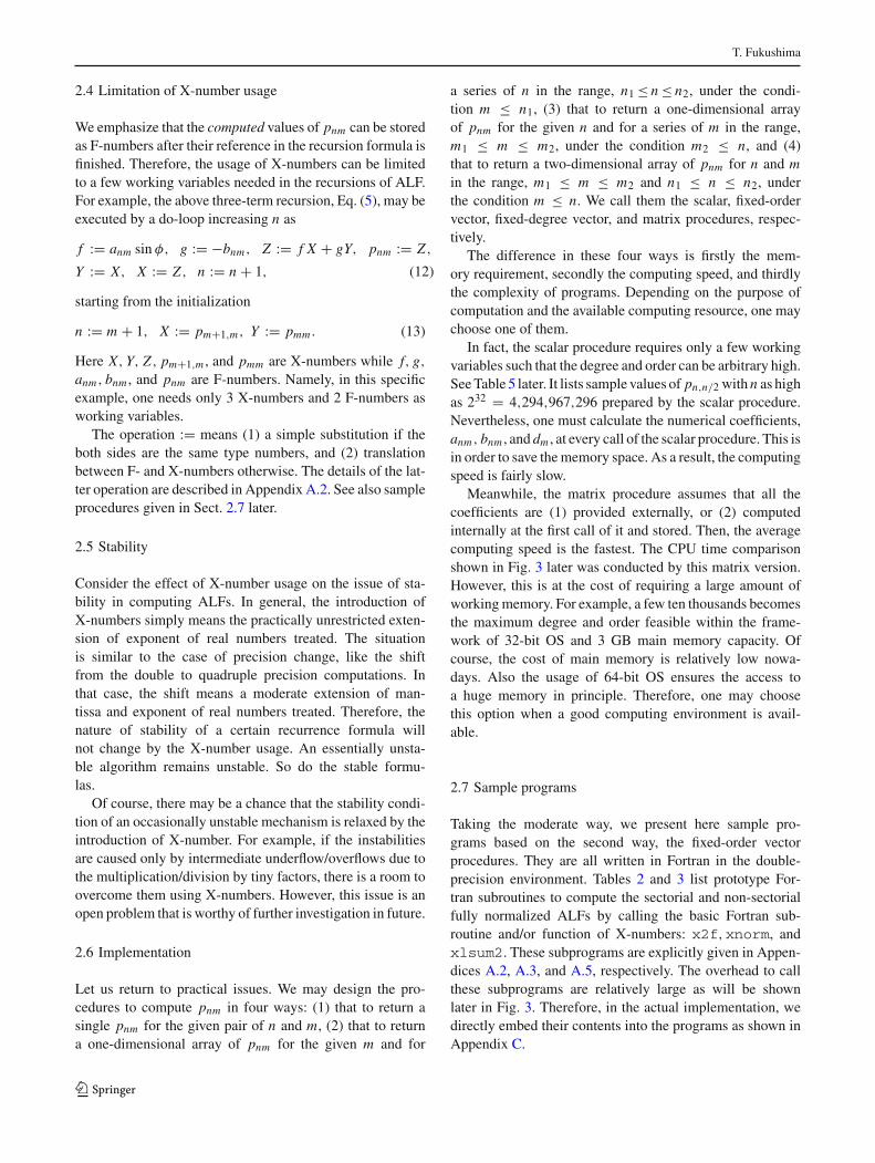
Table 3 Prototype Fortran subroutine to return, for a given order, m, aone-dimensional array of the fully normalized ALFs, pnm , as F-num-bers, pm(n)

subroutine alfmp(t,m,nx,am,bm,psm,ipsm,pm)

integer m,nx,ipsm,n,ix,iy,iz

real*8 t,am(*),bm(*),psm,pm(*),x,y,z,x2f

pm(m)=x2f(psm,ipsm)

if(m.ge.nx) return

y=psm; iy=ipsm; x=(am(m+1)*t)*y; ix=iy

call xnorm(x,ix); pm(m+1)=x2f(x,ix)

do n=m+2,nx

call xlsum2(am(n)*t,-bm(n),x,ix,y,iy,z,iz)

pm(n)=x2f(z,iz); y=x; iy=ix; x=z; ix=iz

enddo

return; end

It requires the seed value, pmm , as an input X-number, i.e.the pair of the significand, psm, and the exponent, ipsm.Called are the three basic subroutine/function of X-numbers:x2f,xnorm, and xlsum2. We assume that the numerical constants,anm ≡ √

(2n + 1)(2n − 1)/((n + m)(n − m)) and bnm ≡ anm/an,m−1,are externally provided as one-dimensional arrays, am(n) and bm(n),respectively. In the program, t ≡ sin φ, and nx is the maximum degreeN

3 Numerical experiments

3.1 Assumptions

We conducted several numerical experiments in order toexamine the cost and performance of the new method in theevaluation of non-zonal fully normalized ALFs. We preparedthree versions of procedures: the scalar, the fixed-order vec-tor, and the matrix ones described in Sect. 2.6. All the com-putation codes were (1) written in Fortran 90, (2) compiled

by the Intel Visual Fortran Composer XE 2011 update 3 withthe level 3 optimization, and (3) executed at a PC with anIntel Core i7-930 CPU and 3 GB main memory run at theclock 2.80 GHz under the 32 bit Windows XP OS.

3.2 Verification

First of all, we examined the validity of the new formulationin the double-precision environment. By comparing with theresults obtained using the standard double-precision arith-metic, we confirmed the correctness of the new method.

Indeed, when the values of fully normalized ALFs arewithin the range of representable numbers of the IEEE754standard, all the computed results obtained by the newmethod coincide with those without the exponent extensionexactly, namely, down to the last bit. This is due to the choiceof the radix as an even integer power of 2, namely, B = 2960.See Appendix A.6.

The coincidence maintains up to the degree 157 in thedouble-precision environment. Beyond that, we observe thatthe result using the standard arithmetic suffers the underflowproblem. Similar results are obtained when we alter the valueof radix B as 2200, 2300, . . ., or 2900 where the coincidencepoint decreases according as the adopted radix decreases.This independence on the radix also supports the correctnessof the new formulation.

As another independent verification, we checked thenumerical values of fully normalized ALFs of some highorder and degree by directly comparing with the resultsobtained by the high precision computation by Mathemat-ica (Wolfram 2003). Table 4 lists the values of P

mn (sin φ)

of n from 21,598 to 21,600, m from 10,798 to 10,800, andφ = π/6.

We prepared 3 × 3 ALFs in order to confirm almost allkinds of their recurrence formulas. They are computed by thefixed-order vector version of the new formulation in the dou-ble-precision environment and by Mathematica in 35 digitscomputation issued by the command

Do[Do[Print[N[(−1) ˆmSqrt[(4n+ 2)(n− m)!/(n+ m)!]LegendreP[n,m,Sin[Pi/6]],35]],{m,10798,10800}], {n,21598,21600}]

The definition of ALF in Mathematica is different from oursby the factor (−1)m . The table indicates that the values com-puted by the new formulation seem to be correct up to 11digits when n and m are a few ten thousands.

3.3 Computational errors

Let us examine the computational errors of the new formu-lation more thoroughly. Hereafter, we set N = M for sim-plicity. First, we show the comparison with the quadruple

123

T. Fukushima

Table 4 Spot check of ALFs computed by the new formulation

n m Pmn (sin φ)

21,598 10,798 −0.7207271824916766

−0.72072718248877284286000605898736874

21,599 −1.849424515663204

+1.8494245156622562685155553139338132

21,600 −1.414683620040851

−1.4146836200426610005610639323498268

21,598 10,799 +1.414887096513534

+1.4148870965153789531023961963339046

21,599 −0.2157080798968343

−0.21570807989372272466504390412379465

21,600 −1.663935814577199

−1.6639358145754512863740569125023061

21,598 10,800 +1.663992935067548

+1.6639929350658376344061443702751905

21,599 +1.705687301913355

+1.7056873019144002958924638199742966

21,600 +0.3055907911155904

+0.30559079111850769219467081153397780

Shown are the numerical values of the fully normalized ALFs of highdegree and order for the latitude φ = π/6. The values are computedby the fixed-order vector version of the new formulation in the double-precision environment and using Mathematica (Wolfram 2003) with 35significant digits

-16

-15

-14

-13

-12

-11

0 10 20 30 40 50 60 70 80 90

log 1

0δA

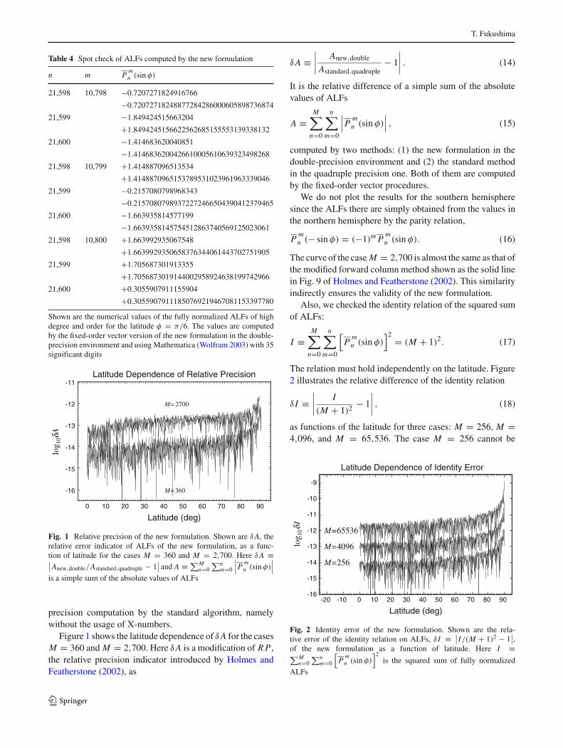
Latitude (deg)

Latitude Dependence of Relative Precision

M= 2700

M=360

Fig. 1 Relative precision of the new formulation. Shown are δA, therelative error indicator of ALFs of the new formulation, as a func-tion of latitude for the cases M = 360 and M = 2,700. Here δA ≡∣∣Anew,double/Astandard,quadruple − 1

∣∣ and A ≡ ∑Mn=0

∑nm=0

∣∣∣Pmn (sin φ)

∣∣∣is a simple sum of the absolute values of ALFs

precision computation by the standard algorithm, namelywithout the usage of X-numbers.

Figure 1 shows the latitude dependence of δA for the casesM = 360 and M = 2,700. Here δA is a modification of R P ,the relative precision indicator introduced by Holmes andFeatherstone (2002), as

δA ≡∣∣∣∣ Anew,double

Astandard,quadruple− 1

∣∣∣∣ . (14)

It is the relative difference of a simple sum of the absolutevalues of ALFs

A ≡M∑

n=0

n∑m=0

∣∣∣Pmn (sin φ)

∣∣∣ , (15)

computed by two methods: (1) the new formulation in thedouble-precision environment and (2) the standard methodin the quadruple precision one. Both of them are computedby the fixed-order vector procedures.

We do not plot the results for the southern hemispheresince the ALFs there are simply obtained from the values inthe northern hemisphere by the parity relation,

Pmn (− sin φ) = (−1)m P

mn (sin φ). (16)

The curve of the case M = 2,700 is almost the same as that ofthe modified forward column method shown as the solid linein Fig. 9 of Holmes and Featherstone (2002). This similarityindirectly ensures the validity of the new formulation.

Also, we checked the identity relation of the squared sumof ALFs:

I ≡M∑

n=0

n∑m=0

[P

mn (sin φ)

]2 = (M + 1)2. (17)

The relation must hold independently on the latitude. Figure2 illustrates the relative difference of the identity relation

δ I ≡∣∣∣∣ I

(M + 1)2 − 1

∣∣∣∣ , (18)

as functions of the latitude for three cases: M = 256, M =4,096, and M = 65,536. The case M = 256 cannot be

-16

-15

-14

-13

-12

-11

-10

-9

-20 -10 0 10 20 30 40 50 60 70 80 90

log 1

0δI

Latitude (deg)

Latitude Dependence of Identity Error

M=65536

M=4096

M=256

Fig. 2 Identity error of the new formulation. Shown are the rela-tive error of the identity relation on ALFs, δ I ≡ ∣∣I/(M + 1)2 − 1

∣∣,of the new formulation as a function of latitude. Here I ≡∑M

n=0∑n

m=0

[P

mn (sin φ)

]2is the squared sum of fully normalized

ALFs

123

Numerical computation of spherical harmonics

0

5

10

15

20

25

2 3 4 5 6 7 8 9 10 11 12 13 14

CP

U T

ime

(Uni

t: ns

)

log2M

Averaged CPU Time of ALF Computation

Standard Exponent

Extended Exponent (Embedded)

Extended Exponent (Prototype)

Fig. 3 Size dependence of CPU time of ALF computation. Shown arethe averaged CPU times of three programs to compute the fully nor-malized ALFs

correctly computed by the standard method unless using asuitable trick such as the global pre-scaling by a factor of theorder of 10250. Also the cases M = 4,096 and M = 65,536are difficult to be evaluated properly without extending expo-nents as in the new formulation. These curves numericallyconfirm the correctness of the new formulation.

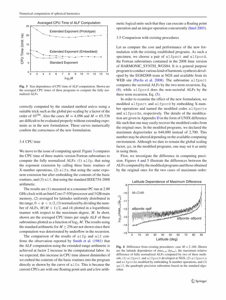
3.4 CPU time

We move to the issue of computing speed. Figure 3 comparesthe CPU time of three matrix version Fortran subroutines tocompute the fully normalized ALFs: (1) alfp, that usingthe exponent extension by calling three basic routines ofX-number operations, (2) alfx, that using the same expo-nent extension but after embedding the contents of the basicroutines, and (3) alf, that using the standard IEEE754-2008arithmetic.

The results are (1) measured at a consumer PC run at 2.80GHz clock with an Intel Core i7-930 processor and 3 GB mainmemory, (2) averaged for latitudes uniformly distributed inthe range, 0 < φ < π/2, (3) normalized by dividing the num-ber of ALFs, M(M + 1)/2, and (4) plotted in a logarithmicmanner with respect to the maximum degree, M . In short,shown are the averaged CPU times per single ALF of thesesubroutines plotted as a function of log2 M . The results usingthe standard arithmetic for M ≥ 256 are not shown since theircomputation was deteriorated by underflow in the recursion.

The comparison of the results of alfp and alf con-firms the observation reported by Smith et al. (1981) thatthe ALF computation using the extended-range arithmetic isachieved at factor 2 increase in the computational labor. Aswe expected, this increase in CPU time almost diminishes ifwe embed the contents of the basic routines into the programdirectly as shown by the curve of alfx. This is because thecurrent CPUs are with one floating point unit and a few arith-

metic logical units such that they can execute a floating pointoperation and an integer operation concurrently (Intel 2003).

3.5 Comparison with existing procedures

Let us compare the cost and performance of the new for-mulation with the existing established programs. As such aspecimen, we choose a pair of alfpsct and alfpord,the Fortran subroutines contained in the 2008 June versionof HARMONIC_SYNTH_WGS84. It is a general purposeprogram to conduct various kind of harmonic synthesis devel-oped by the EGM2008 team at NGS and available from itsWEB site (Pavlis et al. 2008). The subroutine alfpsctcomputes the sectorial ALFs by the two-term recursion, Eq.(8), while alfpord does the non-sectorial ALFs by thethree-term recursion, Eq. (5).

In order to examine the effect of the new formulation, wemodified alfpsct and alfpord by embedding X-num-ber operations and named the modified codes alfpsctxand alfpordx, respectively. The details of the modifica-tion are given in Appendix D in the form of UNIX differencefile such that one may easily recover the modified codes fromthe original ones. In the modified programs, we declared themaximum degree/order as 648,000 instead of 2,700. Thisnumber may be altered depending on the available computingenvironment. Although we dare to remain the global scalingfactor, gs, in the modified programs, one may set it as unityin using them.

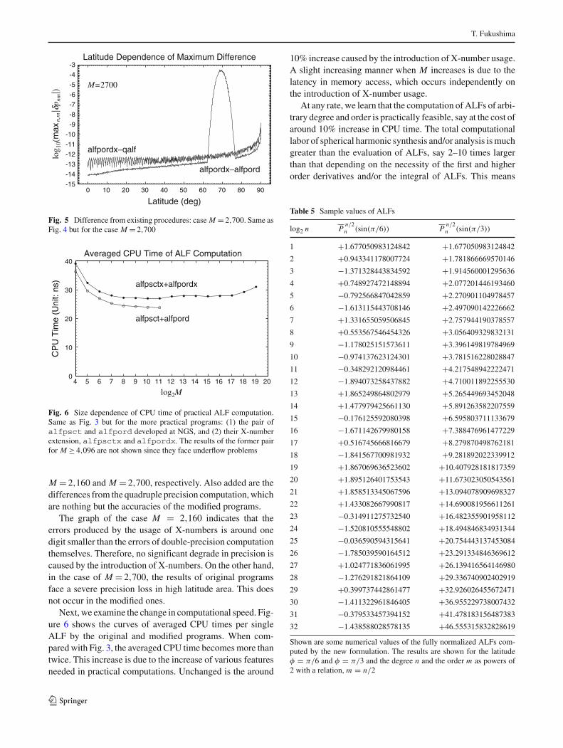
First, we investigate the difference in computing preci-sion. Figures 4 and 5 illustrate the differences between theALFs computed by the modified programs and those obtainedby the original ones for the two cases of maximum order:

-15

-14

-13

-12

-11

-10

-9

0 10 20 30 40 50 60 70 80 90

log 1

0(m

axn,

m| δ

p nm

|)

Latitude (deg)

Latitude Dependence of Maximum Difference

M=2160

alfpordx−qalf

alfpordx−alfpord

Fig. 4 Difference from existing procedures: case M = 2,160. Shownare the latitude dependence of maxn,m |δpnm |, the maximum relativedifference of fully normalized ALFs computed by two of three meth-ods; (1) alfpsct and alfpord developed at NGS, (2) alfpsctxand alfpordx modified by embedding X-number operations, and (3)qalf, the quadruple precision subroutine based on the standard algo-rithm

123

T. Fukushima

-15

-14

-13

-12

-11

-10

-9

-8

-7

-6

-5

-4

-3

0 10 20 30 40 50 60 70 80 90

log 1

0(m

axn,

m| δ

p nm

|)

Latitude (deg)

Latitude Dependence of Maximum Difference

M=2700

alfpordx−qalf

alfpordx−alfpord

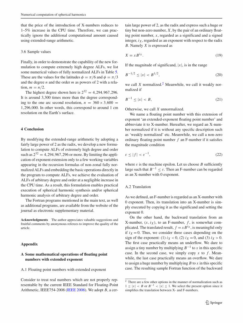
Fig. 5 Difference from existing procedures: case M = 2,700. Same asFig. 4 but for the case M = 2,700

0

10

20

30

40

4 5 6 7 8 9 10 11 12 13 14 15 16 17 18 19 20

CP

U T

ime

(Uni

t: ns

)

log2M

Averaged CPU Time of ALF Computation

alfpsct+alfpord

alfpsctx+alfpordx

Fig. 6 Size dependence of CPU time of practical ALF computation.Same as Fig. 3 but for the more practical programs: (1) the pair ofalfpsct and alfpord developed at NGS, and (2) their X-numberextension, alfpsctx and alfpordx. The results of the former pairfor M ≥ 4,096 are not shown since they face underflow problems

M = 2,160 and M = 2,700, respectively. Also added are thedifferences from the quadruple precision computation, whichare nothing but the accuracies of the modified programs.

The graph of the case M = 2,160 indicates that theerrors produced by the usage of X-numbers is around onedigit smaller than the errors of double-precision computationthemselves. Therefore, no significant degrade in precision iscaused by the introduction of X-numbers. On the other hand,in the case of M = 2,700, the results of original programsface a severe precision loss in high latitude area. This doesnot occur in the modified ones.

Next, we examine the change in computational speed. Fig-ure 6 shows the curves of averaged CPU times per singleALF by the original and modified programs. When com-pared with Fig. 3, the averaged CPU time becomes more thantwice. This increase is due to the increase of various featuresneeded in practical computations. Unchanged is the around

10% increase caused by the introduction of X-number usage.A slight increasing manner when M increases is due to thelatency in memory access, which occurs independently onthe introduction of X-number usage.

At any rate, we learn that the computation of ALFs of arbi-trary degree and order is practically feasible, say at the cost ofaround 10% increase in CPU time. The total computationallabor of spherical harmonic synthesis and/or analysis is muchgreater than the evaluation of ALFs, say 2–10 times largerthan that depending on the necessity of the first and higherorder derivatives and/or the integral of ALFs. This means

Table 5 Sample values of ALFs

log2 n Pn/2n (sin(π/6)) P

n/2n (sin(π/3))

1 +1.677050983124842 +1.677050983124842

2 +0.943341178007724 +1.781866669570146

3 −1.371328443834592 +1.914560001295636

4 +0.748927472148894 +2.077201446193460

5 −0.792566847042859 +2.270901104978457

6 −1.613115443708146 +2.497090142226662

7 +1.331655059506845 +2.757944190378557

8 +0.553567546454326 +3.056409329832131

9 −1.178025151573611 +3.396149819784969

10 −0.974137623124301 +3.781516228028847

11 −0.348292120984461 +4.217548942222471

12 −1.894073258437882 +4.710011892255530

13 +1.865249864802979 +5.265449693452048

14 +1.477979425661130 +5.891263582207559

15 −0.176125592080398 +6.595803711133679

16 −1.671142679980158 +7.388476961477229

17 +0.516745666816679 +8.279870498762181

18 −1.841567700981932 +9.281892022339912

19 +1.867069636523602 +10.407928181817359

20 +1.895126401753543 +11.673023050543561

21 +1.858513345067596 +13.094078909698327

22 +1.433082667990817 +14.690081956611261

23 −0.314911275732540 +16.482355901958112

24 −1.520810555548802 +18.494846834931344

25 −0.036590594315641 +20.754443137453084

26 −1.785039590164512 +23.291334846369612

27 +1.024771836061995 +26.139416564146980

28 −1.276291821864109 +29.336740902402919

29 +0.399737442861477 +32.926026455672471

30 −1.411322961846405 +36.955229738007432

31 −0.379533457394152 +41.478183156487383

32 −1.438588028578135 +46.555315832828619

Shown are some numerical values of the fully normalized ALFs com-puted by the new formulation. The results are shown for the latitudeφ = π/6 and φ = π/3 and the degree n and the order m as powers of2 with a relation, m = n/2

123

Numerical computation of spherical harmonics

that the price of the introduction of X-numbers reduces to1–5% increase in the CPU time. Therefore, we can prac-tically ignore the additional computational amount causedusing extended-range arithmetic.

3.6 Sample values

Finally, in order to demonstrate the capability of the new for-mulation to compute extremely high degree ALFs, we listsome numerical values of fully normalized ALFs in Table 5.These are the values for the latitudes φ = π/6 and φ = π/3and the degree n and the order m as powers of 2 with a rela-tion, m = n/2.

The highest degree shown here is 232 = 4,294,967,296.It is around 3,300 times more than the degree correspond-ing to the one arc second resolution, n = 360 × 3,600 =1,296,000. In other words, this correspond to around 1 cmresolution on the Earth’s surface.

4 Conclusion

By modifying the extended-range arithmetic by adopting afairly large power of 2 as the radix, we develop a new formu-lation to compute ALFs of extremely high degree and ordersuch as 232 = 4,294,967,296 or more. By limiting the appli-cation of exponent extension only to a few working variablesappearing in the recursion formulas of non-zonal fully nor-malized ALFs and embedding the basic operations directly inthe program to compute ALFs, we achieve the evaluation ofALFs of arbitrary degree and order at a negligible increase inthe CPU time. As a result, this formulation enables practicalexecution of spherical harmonic synthesis and/or sphericalharmonic analysis of arbitrary degree and order.

The Fortran programs mentioned in the main text, as wellas additional programs, are available from the website of thejournal as electronic supplementary material.

Acknowledgments The author appreciates valuable suggestions andfruitful comments by anonymous referees to improve the quality of thearticle.

Appendix

A Some mathematical operations of floating pointnumbers with extended exponent

A.1 Floating point numbers with extended exponent

Consider to treat real numbers which are not properly rep-resentable by the current IEEE Standard for Floating-PointArithmetic, IEEE754-2008 (IEEE 2008). We adopt B, a cer-

tain large power of 2, as the radix and express such a huge ortiny but non-zero number, X , by the pair of an ordinary float-ing point number, x , regarded as a significand and a signedinteger, iX , regarded as an exponent with respect to the radixB. Namely X is expressed as

X = x BiX . (19)

If the magnitude of significand, |x |, is in the range

B−1/2 ≤ |x | < B1/2, (20)

we call X normalized.2 Meanwhile, we call it weakly nor-malized if

B−1 ≤ |x | < B, (21)

Otherwise, we call X unnormalized.We name a floating point number with this extension of

exponent ‘an extended-exponent floating point number’ andabbreviate it to X-number. Hereafter, we regard an X-num-ber normalized if it is without any specific description suchas ‘weakly normalized’ etc. Meanwhile, we call a non-zeroordinary floating point number f an F-number if it satisfiesthe magnitude condition

ε ≤ | f | < ε−1, (22)

where ε is the machine epsilon. Let us choose B sufficientlylarge such that B−1 ≤ ε. Then an F-number can be regardedas an X-number with 0 exponent.

A.2 Translation

As we defined, an F-number is regarded as an X-number with0 exponent. Then, its translation into an X-number is sim-ply executed by copying it as the significand and setting theexponent 0.

On the other hand, the backward translation from anX-number, (x, iX ), to an F-number, f , is somewhat com-plicated. The translated result, f = x BiX , is meaningful onlyif iX = 0. Thus, we consider three cases depending on thesign of the exponent: (1) iX < 0, (2) iX = 0, and (3) iX > 0.The first case practically means an underflow. We dare toassign a tiny number by multiplying B−1 to x in this specificcase. In the second case, we simply copy x to f . Mean-while, the last case practically means an overflow. We dareto assign a huge number by multiplying B to x in this specificcase. The resulting sample Fortran function of the backward

2 There are a few other options in the manner of normalization such as1 ≤ |x | < B or B−1 < |x | ≤ 1. We select the present option since itsimplifies the translation between X- and F-numbers.

123

T. Fukushima

Table 6 Fortran function to translate an X-number into an F-number

real*8 function x2f(x,ix)

integer ix,IND

real*8 x,BIG,BIGI

parameter (IND=960,BIG=2.d0**IND,BIGI=2.d0**(-IND))

if(ix.eq.0) then

x2f=x

elseif(ix.lt.0) then

x2f=x*BIGI

else

x2f=x*BIG

endif

return; end

The radix B and its reciprocal B−1 are named BIG and BIGI in theprogram. An integer constant IND is the index of power of 2 to definethe radix

Table 7 Fortran subroutine to normalize a weakly normalized X-num-ber

subroutine xnorm(x,ix)

integer ix,IND

real*8 x,w,BIG,BIGI,BIGS,BIGSI

parameter (IND=960,BIG=2.d0**IND,BIGI=2.d0**(-IND))

parameter (BIGS=2.d0**(IND/2),BIGSI=2.d0**(-IND/2))

w=abs(x)

if(w.ge.BIGS) then

x=x*BIGI; ix=ix+1

elseif(w.lt.BIGSI) then

x=x*BIG; ix=ix-1

endif

return; end

The constants related with the normalization bounds, B1/2 and B−1/2,are termed as BIGS and BIGSI, respectively

translation in the double-precision environment is listed inTable 6.

A.3 Normalization

During the mathematical operations of X-numbers, we fre-quently encounter with a situation where the computedX-number is weakly normalized. We need to normalize it toassure the following operations are appropriately conductedsince we design the algorithm of mathematical operationsunder the condition that X-numbers are all normalized. Theactual normalization is realized by two conditional judg-ments and, if necessary, the combination of multiplicationof the significand by B or B−1, and a decrement or incre-ment of the exponent, iX . The resulting program is describedin Table 7.

A.4 F-number multiplication

The product of an F-number, f , and an X-number, X ≡(x, iX ), is formally computed as

f X = f x BiX . (23)

The conditions of the multiplicands, ε ≤ | f | < ε−1 andB−1/2 ≤ |x | < B1/2, lead to an inequality of the significandof the product as εB−1/2 ≤ | f x | < ε−1 B1/2. Therefore,in order to avoid an underflow and an overflow during thecomputation, we must choose B sufficiently small such thatδ < εB−1/2 and ε−1 B1/2 < ω. Since the inequality on | f x |means that the formal expression is weakly normalized, wenormalize it using xnorm described in the above.

A.5 Two-term linear sum

Let us consider to compute the two-term linear sum ofX-numbers with non-zero3 F-number coefficients:

Z = f X + gY. (24)

An orthodox way is to split the process to two F-number mul-tiplications and one X-number summation. Here, we examinea direct way in order to save the computational time.

Assume the order condition of the exponents as iX ≥ iY .If not, the condition would be satisfied by exchanging the pairof f and X and that of g and Y . Then, we obtain a formalexpression of the linear sum as

Z =(

f x + gy BiY −iX)

BiX . (25)

Since the calculated significand is unnormalized in general,we consider its normalization case by case.

First, consider the case iY − iX ≤ −2. let us make B suf-ficiently large such that B > ε−3. Then, an inequality on themagnitude of two summands is obtained as∣∣∣gy BiY −iX

∣∣∣ < ε−1 B−3/2 < ε2 B−1/2 ≤ ε | f x | . (26)

Since the magnitude of the smaller summand is less than themachine epsilon times that of the larger one, we can ignorethe contribution of the smaller summand as

Z = f X. (27)

This is achieved by the F-number multiplication explainedin Appendix A.4.

Next, consider the case iY − iX = −1. This time, theinequalities of the summands are εB−3/2 ≤ ∣∣gy BiY −iX

∣∣ <

ε−1 B−1/2 and εB−1/2 ≤ | f x | < ε−1 B1/2. Then, except avery rare case that the computed significand happens to be

3 If f or g is zero, the computation reduces to the F-number multipli-cation already explained in Appendix A.4.

123

Numerical computation of spherical harmonics

Table 8 Fortran subroutine to compute the two-term linear sum of X-numbers with F-number coefficients

subroutine xlsum2(f,g,x,ix,y,iy,z,iz)

integer ix,iy,iz,IND,id

real*8 f,g,x,y,z,BIGI

parameter (IND=960,BIGI=2.d0**(-IND))

id=ix-iy

if(id.eq.0) then

z=f*x+g*y; iz=ix

elseif(id.eq.1) then

z=f*x+g*(y*BIGI); iz=ix

elseif(id.eq.-1) then

z=g*y+f*(x*BIGI); iz=iy

elseif(id.gt.1) then

z=f*x; iz=ix

else

z=g*y; iz=iy

endif

call xnorm(z,iz)

return; end

exactly equal to 0, which we ignore in practical computa-tions, the significand satisfies an inequality as

ε2 B−1/2 ≤∣∣∣ f x + gy B−1

∣∣∣ < ε−1 B1/2(

1 + B−1)

. (28)

Since the lower and upper bounds satisfy the inequalitiesB−1 < ε2 B−1/2 and ε−1 B1/2

(1 + B−1

)< B, we find that

the significand is weakly normalized. Therefore, we normal-ize the significand after its calculation.

Finally, consider the last case iX = iY . Again, we neglecta very rare chance of the zero value significand. Then, theabove inequality changes a little as

ε2 B−1/2 ≤ | f x + gy| < 2ε−1 B1/2. (29)

At any rate, unchanged is a fact that the significand is weaklynormalized. Thus, we conduct the same normalization as inthe previous case. The resulting whole algorithm of the sum-mation is implemented in a sample Fortran subroutine shownin Table 8.

A.6 Choice of radix

Let us summarize the conditions on the radix B required in theprevious subsections: B−1 < ε, δ < εB−1/2, ε−1 B1/2 < ω,and ε−3 < B. These are unified as

ε−3 < B < ω, (30)

since the upper bounds, ε2δ−2 and ε−2ω2, exceed ω. In orderto avoid the introduction of unnecessary round-off error bythe multiplication of B or B−1 and in the comparison with

Table 9 Fortran subroutine to return a one-dimensional array of thefully normalized sectorial ALFs in X-numbers

subroutine alfsx(u,mx,d,ps,ips)

integer mx,ips(*),IND,ix,m

parameter (IND=960)

real*8 u,d(*),ps(*),BIG,BIGI,BIGS,BIGSI,ROOT3,x,y

parameter (BIG=2.d0**IND,BIGI=2.d0**(-IND))

parameter (BIGS=2.d0**(IND/2),BIGSI=2.d0**(-IND/2))

parameter (ROOT3=1.7320508075688773d0)

x=ROOT3*u; ix=0; ps(1)=x; ips(1)=ix

do m=2,mx

x=(d(m)*u)*x; y=abs(x)

if(y.ge.BIGS) then

x=x*BIGI; ix=ix+1

elseif(y.lt.BIGSI) then

x=x*BIG; ix=ix-1

endif

ps(m)=x; ips(m)=ix

enddo

return; end

√B or 1/

√B, it is better to set B as an even power of 2. Con-

sidering these, we adopt as B the following numbers beingsomewhat smaller than ω:

Bsingle = 2120 ≈ 1.33 × 1036, (31)

Bdouble = 2960 ≈ 9.75 × 10288, (32)

Bquadruple = 216000 ≈ 3.02 × 104816. (33)

Refer to Table 1.

B F-number computation of integral of ALF

Let us consider to compute definite integrals of the fully nor-malized ALF with respect to the argument, t = sin φ:

Inm ≡∫ t2

t1P

mn (t)dt. (34)

Usually, they are computed by recursions of the form (Paul1978) as

Inm = fnm In−2,m − gnmqn−1,m, (n ≥ m + 2) (35)

Imm = jm Im−2,m−2 + kmqm−1,m−2, (m ≥ 2) (36)

with the seed values

I00 = t2 − t1, I11 =√

3

2

[t√

1 − t2 + sin−1 t]t2

t1, (37)

where

qnm ≡[(

1 − t2)

Pmn (t)

]t2

t1(38)

123

T. Fukushima

Table 10 Fortran subroutine to return a one-dimensional array of thefully normalized ALFs for a given order using X-numbers

subroutine alfmx(t,m,nx,am,bm,psm,ipsm,pm)

integer IND,m,nx,ipsm,n,id,iw,ix,iy,iz

parameter (IND=960)

real*8 t,am(*),bm(*),psm,pm(*),x,y,w,z

real*8 BIG,BIGI,BIGS,BIGSI

parameter (BIG=2.d0**IND,BIGI=2.d0**(-IND))

parameter (BIGS=2.d0**(IND/2),BIGSI=2.d0**(-IND/2))

x=psm; ix=ipsm

if(ix.eq.0) then

pm(m)=x

elseif(ix.lt.0) then

pm(m)=x*BIGI

else

pm(m)=x*BIG

endif

if(m.ge.nx) return

y=x; iy=ix; x=(am(m+1)*t)*y; ix=iy; w=abs(x)

if(w.ge.BIGS) then

x=x*BIGI; ix=ix+1

elseif(w.lt.BIGSI) then

x=x*BIG; ix=ix-1

endif

if(ix.eq.0) then

pm(m+1)=x

elseif(ix.lt.0) then

pm(m+1)=x*BIGI

else

pm(m+1)=x*BIG

endif

do n=m+2,nx

id=ix-iy

if(id.eq.0) then

z=(am(n)*t)*x-bm(n)*y; iz=ix

elseif(id.eq.1) then

z=(am(n)*t)*x-bm(n)*(y*BIGI); iz=ix

elseif(id.eq.-1) then

z=(am(n)*t)*(x*BIGI)-bm(n)*y; iz=iy

elseif(id.gt.1) then

z=(am(n)*t)*x; iz=ix

else

z=-bm(n)*y; iz=iy

endif

w=abs(z)

if(w.ge.BIGS) then

z=z*BIGI; iz=iz+1

elseif(w.lt.BIGSI) then

z=z*BIG; iz=iz-1

endif

Table 10 continued

if(iz.eq.0) then

pm(n)=z

elseif(iz.lt.0) then

pm(n)=z*BIGI

else

pm(n)=z*BIG

endif

y=x; iy=ix; x=z; ix=iz

enddo

return; end

Table 11 Standard Fortran subroutine to return a one-dimensionalarray of the fully normalized sectorial ALFs

subroutine alfs(u,nx,d,ps)

integer nx,m

real*8 u,d(*),ps(*),ROOT3

parameter (ROOT3=1.7320508075688773d0)

ps(1)=ROOT3*u

do m=2,nx

ps(m)=(d(m)*u)*ps(m-1)

enddo

return; end

Table 12 Standard Fortran subroutine to return a one-dimensionalarray of the fully normalized ALFs for a given order

subroutine alfm(t,m,nx,am,bm,psm,pm)

integer m,nx,n

real*8 t,am(*),bm(*),psm,pm(*)

pm(m)=psm; if(m.ge.nx) return

pm(m+1)=(am(m+1)*t)*psm

do n=m+2,nx

pm(n)=(am(n)*t)*pm(n-1)-bm(n)*pm(n-2)

enddo

return; end

is the partial integral associated with Inm , and

fnm ≡(

n − 2

n + 1

)bnm

= n − 2

n + 1

√(2n + 1)(n + m − 1)(n − m − 1)

(2n − 3)(n + m)(n − m), (39)

gnm ≡ 1

(n + 1)anm= 1

n + 1

√(2n + 1)(2n − 1)

(n + m)(n − m), (40)

jm ≡ 1

2(m + 1)

√m(2m − 1)(2m + 1)

m − 1, (41)

km ≡ 1

2(m + 1)

√2m + 1

m(m − 1), (42)

123

Numerical computation of spherical harmonics

Table 13 Difference of files, alfpsct.f and alfpsctx.f

2,3c2,3

< subroutine alfpsct(nrst,nrfn,thetc,nmax,gs,ider,pmmd0,pmmd1,zero,

< & nmax0)

—

> subroutine alfpsctx(nrst,nrfn,thetc,nmax,gs,ider,pmmd0,ipmmd0,

> & pmmd1,zero,nmax0)

47c47

< c Note that ’nmax’ should never be larger than 2700.

—

> c Note that ’nmax’ should never be larger than 648000.

60c60,61

< parameter(nm=2700,nm1=nm+1)

—

> implicit integer(i-n)

> parameter(nm=648000,nm1=nm+1)

63c64,67

< integer*4 zero(*)

—

> integer zero(*),ipmmd0(nmax0+1,*),IND,ix

> real*8 BIG,BIGI,BIGS,BIGSI,x,absx

> parameter (IND=960,BIG=2.d0**IND,BIGI=2.d0**(-IND))

> parameter (BIGS=2.d0**(IND/2),BIGSI=2.d0**(-IND/2))

65c69

< if (nmax.gt.nmax0.or.nmax0.gt.2700) then

—

> if (nmax.gt.nmax0.or.nmax0.gt.648000) then

68c72

< &’*** Error in s/r alfpsct: nmax > nmax0 or nmax0 > 2700 ***’,

—

> &’*** Error in s/r alfpsctx: nmax > nmax0 or nmax0 > 648000 ***’,

95,103c99

< if (u.eq.0.d0) then

< mmax1 = 1

< elseif (u.eq.1.d0) then

< mmax1 = nmax1

< else

< testm1 = (small - gslog)/dlog10(u) + 1.d0

< if (testm1.gt.xmax1) testm1 = xmax1

< mmax1 = nint(testm1)

< endif ! u

—

> mmax1 = nmax1

109a106

> ipmmd0(n1,nr) = 0

116c113,119

< pmmd0(1,nr) = gs

—

> x = gs; ix = 0

> if (absx.ge.BIGS) then

Table 13 continued

> x = x*BIGI; ix = ix+1

> elseif (absx.lt.BIGSI) then

> x = x*BIG; ix = ix-1

> endif

> pmmd0(1,nr) = x; ipmmd0(1,nr) = ix

119c122,128

< pmmd0(n1,nr) = c(n1)*pmmd0(n1-1,nr)*u

—

> x = (c(n1)*u)*x; absx = abs(x)

> if (absx.ge.BIGS) then

> x = x*BIGI; ix = ix+1

> elseif (absx.lt.BIGSI) then

> x = x*BIG; ix = ix-1

> endif

> pmmd0(n1,nr) = x; ipmmd0(n1,nr) = ix

140c149

< &’*** Error in s/r alfpsct: check that 0<=thetc<=pi ***’,

—

> &’*** Error in s/r alfpsctx: check that 0<=thetc<=pi ***’,

are numerical coefficients depending on n and/or m only. SeePaul (1978) for details.

When m increases, jm and km approach to 1 and 0, respec-tively. Therefore, the sectorial recursion causes no exponen-tial damping nor amplification of the seed values, I00 and I11,both of which are F-numbers. Similarly, when n increaseswhile m is fixed, fnm and gnm tend to 1 and 0, respectively.Therefore, the increasing-degree recursion causes no expo-nential amplification of the sectorial and semi-sectorial val-ues, This means that the recursion can be conducted withoutusing X-numbers as long as the value of ALFs themselvesare provided in F-numbers.

C Sample Fortran programs

Let us present some Fortran subroutines to return ALFs asone dimensional array in the double-precision environment.Table 9 shows that to return X-numbers of pmm , the fullynormalized sectorial ALF. Meanwhile, Table 10 lists that toreturn F-numbers of pnm , the fully normalized ALF of a givenorder m. These are rewritings of the prototype programs listedin Sect. 2.7 by embedding the contents of the basic routinesof X-numbers x2f,xnorm, and xlsum2 given in Appen-dices A.2, A.3, and A.5, respectively. The embedding is inorder to reduce the overhead of calling them. For comparisonpurpose, we also list the same subroutines but without usageof X-numbers in Tables 11 and 12.

123

T. Fukushima

Table 14 Difference of files, alfpord.f and alfpordx.f

2,3c2,3

< subroutine alfpord(nrst,nrfn,thetc,m,nmax,ider,pmmd0,pmmd1,

< & p,p1,p2,uc,tc,uic,uic2,cotc,nmax0)

—

> subroutine alfpordx(nrst,nrfn,thetc,m,nmax,ider,pmmd0,ipmmd0,

> & pmmd1,p,p1,p2,uc,tc,uic,uic2,cotc,nmax0)

76c76

< c Note that ’nmax’ should never be larger than 2700.

—

> c Note that ’nmax’ should never be larger than 648000.

89c89,90

< parameter(nm=2700,nm1=nm+1)

—

> implicit integer(i-n)

> parameter(nm=648000,nm1=nm+1)

95a97,100

> integer ipmmd0(nmax0+1,*),IND,ixx,iy,iz,id

> real*8 BIG,BIGI,BIGS,BIGSI,x,y,z,absx,fx,gx

> parameter (IND=960,BIG=2.d0**IND,BIGI=2.d0**(-IND))

> parameter (BIGS=2.d0**(IND/2),BIGSI=2.d0**(-IND/2))

102c107

< if (nmax.gt.nmax0.or.nmax0.gt.2700) then

—

> if (nmax.gt.nmax0.or.nmax0.gt.648000) then

105c110

< &’*** Error in s/r alfpord: nmax > nmax0 or nmax0 > 2700 ***’,

—

> &’*** Error in s/r alfpordx: nmax > nmax0 or nmax0 > 648000 ***’,

113c118

< 6001 format(///5x,’*** Error in s/r alfpord: m > Nmax ***’,

—

> 6001 format(///5x,’*** Error in s/r alfpordx: m > Nmax ***’,

162,163c167,192

< p(m1,nr) = pmmd0(m1,nr)

< p(m2,nr) = rt(m1*2+1)*tc(nr)*p(m1,nr)

—

> x = pmmd0(m1,nr); ixx = ipmmd0(m1,nr); absx = abs(x)

> if (absx.ge.BIGS) then

> x = x*BIGI; ixx = ixx+1

> elseif (absx.lt.BIGSI) then

> x = x*BIG; ixx = ixx-1

> endif

> if (ixx.eq.0) then

> p(m1,nr) = x

> elseif (ixx.lt.0) then

> p(m1,nr) = x*BIGI

> else

> p(m1,nr) = x*BIG

> endif

Table 14 continued

> y = x; iy = ixx; x = (rt(m1*2+1)*tc(nr))*y; ixx = iy; absx = abs(x)

> if (absx.ge.BIGS) then

> x = x*BIGI; ixx = ixx+1

> elseif (absx.lt.BIGSI) then

> x = x*BIG; ixx = ixx-1

> endif

> if (ixx.eq.0) then

> p(m2,nr) = x

> elseif (ixx.lt.0) then

> p(m2,nr) = x*BIGI

> else

> p(m2,nr) = x*BIG

> endif

165c194,218

< p(n1,nr) = a(n1)*tc(nr)*p(n1-1,nr)-b(n1)*p(n1-2,nr)

—

> fx = a(n1)*tc(nr); gx = -b(n1); id = ixx-iy

> if (id.eq.0) then

> z = fx*x+gx*y; iz = ixx

> elseif (id.eq.1) then

> z = fx*x+gx*(y*BIGI); iz = ixx

> elseif (id.eq.-1) then

> z = gx*y+fx*(x*BIGI); iz = iy

> elseif (id.gt.1) then

> z = fx*x; iz = ixx

> else

> z = gx*y; iz = iy

> endif

> y = x; iy = ixx; x = z; ixx = iz; absx = abs(x)

> if (absx.ge.BIGS) then

> x = x*BIGI; ixx = ixx+1

> elseif (absx.lt.BIGSI) then

> x = x*BIG; ixx = ixx-1

> endif

> if (ixx.eq.0) then

> p(n1,nr) = x

> elseif (ixx.lt.0) then

> p(n1,nr) = x*BIGI

> else

> p(n1,nr) = x*BIG

> endif

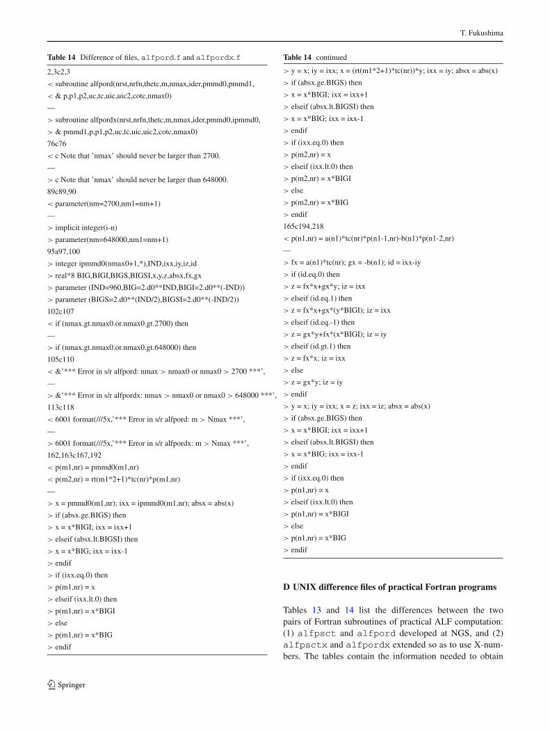
D UNIX difference files of practical Fortran programs

Tables 13 and 14 list the differences between the twopairs of Fortran subroutines of practical ALF computation:(1) alfpsct and alfpord developed at NGS, and (2)alfpsctx and alfpordx extended so as to use X-num-bers. The tables contain the information needed to obtain

123

Numerical computation of spherical harmonics

the latter programs from the former in the format of UNIXdifference file.

In the difference files, the command line “J1(,J2)cK1(,K2)” means changing the line(s) J1 (to J2) in the origi-nal file to the line(s) K1 (to K2) in the modified file. Thelines to be removed from the original file are indicated afterthe sign “<” while those to be added to create the modifiedfile are shown after the symbol “>”.

There exists a new input/output argument,ipmmd0, in themodified subroutines. It is the one-dimensional array con-taining the X-number exponents of the sectorial ALFs. Oneshould declare it and allocate its memory in the programscalling the modified subroutines. Also, in the modified pro-grams, we provisionally altered nm, the size of one-dimen-sional arrays used, from 2,700 to 648,000. This number maybe changed depending on the memory allowance.

References

Bosch W (2000) On the computation of derivatives of Legendre func-tions. Phys Chem Earth 25:655–659

Brendt RP (1978) A Fortran multiple-precision arithmetic package.ACM Trans Math Softw 4:57–70

Casotto S, Fantino E (2007) Evaluation of methods for spherical har-monic synthesis of the gravitational potential and its gradients.Adv Space Res 40:69–75

Cooley JW, Tukey JW (1965) An algorithm for the machine calculationof complex Fourier series. Math Comp 19:297–301

Deprit A (1979) Note on the summation of Legendre series. CelestMech Dyn Astron 20:319–323

Fantino E, Casotto S (2009) Methods of harmonic synthesis for globalgeopotential models and their first-, second- and third-order gra-dients. J Geod 83:595–619

Gleason DM (1985) Partial sums of Legendre series via Clenshaw sum-mation. Manuscr Geod 10:115–130

Goldberg D (1991) What every computer scientist should know aboutfloating-point arithmetic. ACM Comput Surv 23:5–48

Heiskanen WA, Moritz H (1967) Physical geodesy. Freeman and Co,San Francisco

Holmes SA, Featherstone WE (2002) A unified approach to the Clen-shaw summation and the recursive computation of very highdegree and order normalized associated Legendre functions. JGeod 76:279–299

IEEE Comp Soc (2008) IEEE standard for floating-point arithmetic.IEEE Std 754 rev

Intel (2003) Intel hyper-threading technology technical user’s guide.Intel Corp

Jekeli C, Lee JK, Kwon JH (2007) On the computation and approx-imation of ultra-high-degree spherical harmonic series. J Geod81:603–615

Kaula WM (2000) Theory of satellite geodesy: applications of satellitesto geodesy. Dover, Mineora

Kellog OD (1929) Foundations of potential theory. Springer, BerlinLozier DW, Smith JM (1981) Algorithm 567 extended-range arithmetic

and normalized Legendre polynomials. ACM Trans Math Softw7:141–146

Olver FWJ, Lozier DW, Boisvert RF, Clark, CW (eds) (2010) NISThandbook of mathematical functions. Cambridge University Press,Cambridge. http://dlmf.nist.gov/

Paul MK (1978) Recurrence relations for integrals of associated Legen-dre functions. Bull Geod 52:177–190

Pavlis NK, Holmes SA, Kenyon SC, Factor JK (2008) An Earthgravitational model to degree 2160: EGM2008. Presented at the2008 General Assembly of the European Geosciences Union,Vienna, Austria, April 13–18, 2008. http://earth-info.nga.mil/GandG/wgs84/gravitymod/egm2008/index.html

Smith JM, Olver FWJ, Lozier DW (1981) Extended-range arithmeticand normalized Legendre polynomials. ACM Trans Math Softw7:93–105

Tscherning CC, Poder K (1982) Some geodetic applications of Clen-shaw summation. Boll Geofis Sci Aff 4:351–364

Tscherning CC, Rapp RH, Goad C (1983) A comparison of methodsfor computing gravimetric quantities from high degree sphericalharmonic expansions. Manuscr Geod 8:249–272

Wenzel G (1998) Ultra-high degree geopotential models GPM98A, B,and C to degree 1800. Paper presented to the joint meeting of theInternational Gravity Commission and International Geoid Com-mission, 7–12 September, Trieste

Wittwer T, Klees R, Seitz K, Heck B (2008) Ultra-high degree sphericalharmonic analysis and synthesis using extended-range arithmetic.J Geod 82:223–229

Wolfram S (2003) The mathematica book, 5th edn. Wolfram ResearchInc./Cambridge University Press, Cambridge

123