Orbit classification in arbitrary 2D and 3D potentials

Orbit classification in arbitrary 2D and 3D potentials

Daniel D. Carpintero1;2 and Luis A. Aguilar1

1Observatorio Astronomico Nacional, IAUNAM Ensenada, Apdo. postal 877, 22800 Ensenada, Mexico2Facultad de Ciencias Astronomicas y Geofısicas, Universidad Nacional de La Plata, Paseo del bosque S/N, 1900 La Plata, Argentina

Accepted 1997 November 3. Received 1997 September 10; in original form 1996 October 9

A B S T R A C TA method of classifying generic orbits in arbitrary 2D and 3D potentials is presented. It isbased on the concept of spectral dynamics introduced by Binney & Spergel that uses theFourier transform of the time series of each coordinate. The method is tested using a number ofpotentials previously studied in the literature and is shown to distinguish correctly betweenregular and irregular orbits, to identify the various families of regular orbits (boxes, loops,tubes, boxlets, etc.), and to recognize the second-rank resonances that bifurcate from them.The method returns the position of the potential centre and, for 2D potentials, the orientation ofthe principal axes as well, should this be unknown. A further advantage of the method is that ithas been encoded in a FORTRAN program that does not require user intervention, except for ‘finetuning’ of search parameters that define the numerical limits of the code. The automaticcharacter makes the program suitable for classifying large numbers of orbits.

Key words: celestial mechanics, stellar dynamics – galaxies: kinematics and dynamics.

1 I N T RO D U C T I O N

Stellar orbits constitute the basic set of building blocks for thedynamics of galaxies. This is so because galaxies are, to a largeextent, collisionless systems and thus orbits are a well-definedconcept. Although the most important function to a modeller isthe phase-space distribution function, it is not the explicit depen-dence on phase-space coordinates, but an implicit one given by anunderlying orbital structure, that is sought after. The fundamentalproblem of determining whether a self-consistent dynamical modelcan be built with a given potential, ultimately depends on the orbitalstructure supported by the potential. In recent times, a new approachto building 3D dynamical models has been developed that expresslymakes use of a suitable exploration of the orbits supported by thepotential (e.g. Schwarzschild 1979; Richstone 1980, 1984; Statler1987; Levison & Richstone 1987; see de Zeeuw 1994, section 3.4,for a review).

Although the Jeans theorem (Jeans 1915) apparently allowsone to bypass detailed orbital knowledge to build self-consistentdynamical models, questions as to irregularity, chaos, and non-analytical integrals of motion, limit its use to integrable systems, orto those cases in which irregular orbits are not important (Binney1982b). Given the proliferation of irregular orbits on more realisticdynamical systems it seems that, in the end, we need to get back to aproper orbital assessment, even if it is only to ensure that the systemcan be modelled without the difficulties introduced by the irregularorbits.

The orbital structure may have a bearing on other importantissues: irregular orbits in a model in which the curvature ofisopotentials changes rapidly with radius may limit its flattening,

as conjectured by Binney (1982a). Even regular orbits may limit theflattening in triaxial systems (Miralda-Escude & Schwarzschild1989; Lees & Schwarzschild 1992; Pfenniger & de Zeeuw 1989;Schwarzschild 1993). The time-scale on which irregular orbitscover their allowed region in phase space may introduce anotherrelaxation time-scale, much shorter than the two-body relaxationtime-scale (Schwarzschild 1993; Merritt & Fridman 1996).

Integrable potentials (e.g. Stackel 1890; Kuzmin 1956; Lynden-Bell 1962; de Zeeuw 1985) provide us with the basic templates forthe most important regular orbits on generic potentials, and aninsight into the way in which other orbits may arise. Their study,however, can carry us some distance only, as the problem of findingthe factors in a potential that give rise to a particular orbitalstructure, or whether it is integrable or not, is still one of thefundamental unsolved problems of dynamics. Thus the study of theorbital structure of potentials of interest in stellar dynamics hasremained an active enterprise (e.g. Binney 1982a and Miralda-Escude & Schwarzschild 1989 for 2D potentials; Schwarzschild1979, 1993, Richstone 1982, Merritt & de Zeeuw 1983, Gerhard &Binney 1985, Lees & Schwarzschild 1992 and Merritt & Fridman1996 for non-rotating 3D potentials; Heisler, Merritt & Schwarz-schild 1982, Mulder & Hooimeyer 1984 and Pfenniger 1984 forrotating 3D potentials; Wilkinson & James 1982, Pfenniger &Friedli 1991, 1993, Hasan, Pfenniger & Norman 1993 for potentialsextracted from N-body systems). In these and related studies, it isimportant to have a tool that can quickly, and efficiently, classify theorbits obtained. Such a tool is the goal of the present work.

In Section 2 we summarize some notions about orbits andmethods to classify them, and a consistent orbit nomenclature ispresented. Section 3 describes the procedure by which lines are

Mon. Not. R. Astron. Soc. 298, 1–21 (1998)

q 1998 RAS

extracted from the Fourier spectra, the first step of our classificationscheme. In Section 4, all the previous information is used to developa spectral classification method for 2D orbits. Section 5 shows howto obtain information about the potential centre and principal axes.Section 6 discusses some numerical points of our classifier. Section7 presents the results obtained for orbits in 2D potentials. In Section8 we extend the spectral classification scheme to 3D orbits. InSection 9 we present results obtained in 3D potentials. Section 10presents our conclusions.

2 P R E L I M I N A RY N OT I O N S

Here we review some notions about orbits, their structure in phasespace, methods of classifying them, orbital resonances and theirrole in parenting orbit families. The basic characteristics of eachorbit that we will use in the spectral classification are identified, andan orbital nomenclature that synthesizes the most important orbitproperties is introduced.

2.1 Integrals of motion and types of orbits

Orbits are shaped, to a large extent, by their isolating integrals(Binney & Tremaine 1987, hereafter BT87, section 3.1.1). Eachsuch integral lowers by one dimension the region open to an orbit. Ifthe number M of isolating integrals equals the number N of degreesof freedom, the orbital manifold is diffeomorphic to an N-dimen-sional torus, i.e. we can find a one-to-one map between the manifoldand the torus that covers both completely (Arnold 1989, chapter 10;Lichtenberg & Lieberman 1992, section 1.3). Such orbits are calledregular and their motion is quasi-periodic. For them we can define aspecial set of canonical coordinates, the so-called action–anglevariables, in which the motion is constant in the actions and there isuniform rotation in the angle variables.

A regular orbit with additional isolating integrals (M > N) isfurther constrained. This occurs when there are resonances betweenthe rotation of two or more angle variables, in which case the orbit isno longer dense on the torus. Since the rotation frequencies in theangle coordinates are fixed on a given orbital manifold, all orbitssharing the same manifold will be identical, except for a phasedifference (even when M ¼ N, there is an infinite number of orbitssharing the same orbital manifold). We thus speak of non-resonant(M ¼ N), and resonant (M > N) orbital tori; although both aredense in the integrable region of phase space, only the formerform a set of non-zero measure.

If there is full resonance (i.e., M ¼ 2N ¹ 1), the orbit closes onitself after a finite number of turns around the torus and it becomesperiodic. Such orbits are very important, because they can generatetheir own family of orbits: if a periodic orbit is stable (BT87, p. 175),neighbouring orbits will move on concentric tori nested around thestable periodic orbit and form an orbital family. A method foridentifying all stable periodic orbits thus gives us the regular orbitalfamilies supported by a given potential. Although numerical meth-ods have been devised (e.g. Contopoulos & Magenant 1985;Pfenniger & Friedli 1993), these require a long, detailed examina-tion of a large set of orbits.

Irregular orbits, on the other hand, do not have such a torus-likestructure. They have, in general, complicated shapes and may bechaotic, in the sense of having exponential divergence of neigh-bouring orbits. Irregular orbits make difficult the construction ofself-consistent models; the ones dense on the energy manifold, forinstance, are limited by the equipotential surfaces, which, except fora spherical configuration, are different in shape from the isodensitysurfaces of the corresponding mass distribution.

2.2 Orbit classification methods

The dimensionality of the region in which an orbit moves is thefeature exploited by a popular method used to classify orbits in 2Dpotentials. The surface of section (SoS) (see e.g. BT87, section 3.3)is usually taken as a 2D cut of phase space. Intersections of an orbitwith this section lie in a region with one dimension less than theoriginal orbital manifold. Thus, in 2D potentials, irregular orbits,open regular orbits, and closed regular orbits define a ‘sea’, a line,and a finite set of points, respectively. Unfortunately, distinguishingamong these cases involves a visual inspection of the section, andthis results in a subjective and time consuming procedure. Besides,this method is not yet generalized to 3D potentials: a 2D section ofthe corresponding 5D energy manifold does not suffice to disen-tangle orbits moving on three or fewer dimensions (regular) fromthose moving on higher dimensions (irregular).

Another, increasingly popular, way to ascertain whether or not anorbit is regular is by the computation of its Lyapunov characteristicexponents (see e.g. Lichtenberg & Lieberman 1992), which give theexponential rate at which nearby trajectories diverge from theoriginal one. It can be shown that a regular orbit has vanishingLyapunov exponents; unfortunately, it is not clear whether anirregular orbit will necessarily have at least a non-zero realexponent. A positive real exponent signals the onset of a moredisordered behaviour called chaos. (Although it is generallyassumed that irregular and chaotic orbits are the same in Hamil-tonian systems, this has not been proven in general.) Anotherdrawback is that their numerical computation is difficult and timeconsuming. Additionally, unlike SoSs and the method to be pre-sented here, the Lyapunov exponents do not give any furtherinformation regarding regular orbits, for instance, whether or notthey are closed (Merritt & Valluri 1996).

There is another technique first introduced in stellar dynamics byBinney & Spergel (1982, 1984), and more recently extended in adifferent form by Laskar (1993), that relies on one of the funda-mental properties of regular orbits: the fact that they move windingon a torus-like manifold and are thus quasi-periodic. Then, theFourier spectra of the time series of the coordinates of a regular orbitshould consist of discrete lines the frequencies of which can beexpressed as integer linear combinations of the frequencies associ-ated to the N angle variables. We will call these latter frequenciesthe base frequencies (BFs) to stress this property. If the orbit isfurther constrained, this will manifest itself in a reduced number ofincommensurate BFs. If the orbit is closed, only one BF will exist.Irregular orbits, not being quasi-periodic, will produce Fourierspectra with lines the frequencies of which cannot be reduced tointeger combinations of less than N frequencies. If the orbit ischaotic, the spectrum will be continuous (Tabor 1989, section4.5.b).

So, if we compute the Fourier transform of the coordinates of anorbit, identify its peaks, extract the corresponding frequencies, andlook for the BFs (if any), then the orbit could be classified. It turnsout that a closer inspection of the Fourier spectrum can furtherdisclose the orbit family to which the orbit belongs as well as theresonance and resonance rank of its parent, so we need first todescribe these orbit families and their resonant parents and examinethe concept of resonance rank.

2.3 Orbit families and rank of resonant parents

We start with 2D potentials. Apart from the trivial case of a particleat rest at the centre of a potential, the simplest orbits are the axial

2 D. D. Carpintero and L. A. Aguilar

q 1998 RAS, MNRAS 298, 1–21

orbits that move along each axis; these orbits are simple loops inphase space and appear as single points at the origin in the SoSorthogonal to them. When they are stable, the circulation of thedaughter orbits around the parent orbit introduces an additionalfrequency which, in general, is not commensurable with the uniqueBF of its parent; these orbits are dense in the nested tori. Additionally,these daughter orbits do not have a fixed sense of rotation around thecentre and are dense within a box-like region in configuration space.Their intersections with an SoS lie on loops that encircle the singlefixed point that corresponds to the axial orbit. We will call these p-boxorbits to emphasize their frequency incommensurability and the factthat they do not circulate around the origin.

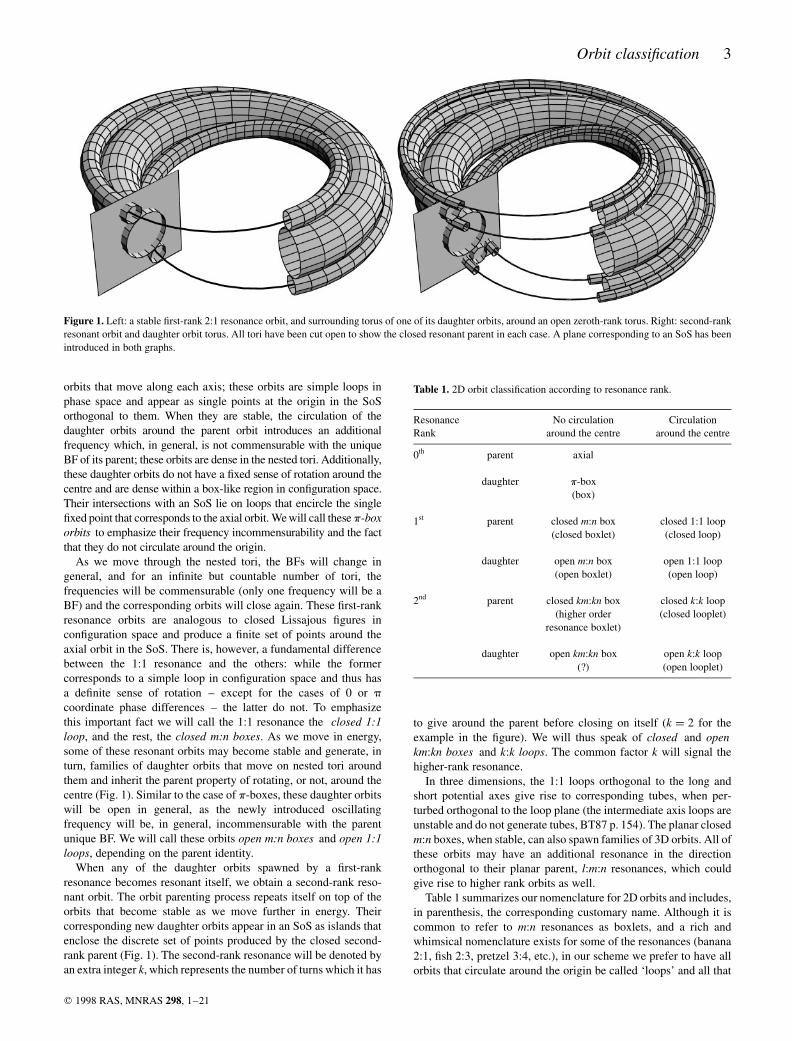
As we move through the nested tori, the BFs will change ingeneral, and for an infinite but countable number of tori, thefrequencies will be commensurable (only one frequency will be aBF) and the corresponding orbits will close again. These first-rankresonance orbits are analogous to closed Lissajous figures inconfiguration space and produce a finite set of points around theaxial orbit in the SoS. There is, however, a fundamental differencebetween the 1:1 resonance and the others: while the formercorresponds to a simple loop in configuration space and thus hasa definite sense of rotation – except for the cases of 0 or pcoordinate phase differences – the latter do not. To emphasizethis important fact we will call the 1:1 resonance the closed 1:1loop, and the rest, the closed m:n boxes. As we move in energy,some of these resonant orbits may become stable and generate, inturn, families of daughter orbits that move on nested tori aroundthem and inherit the parent property of rotating, or not, around thecentre (Fig. 1). Similar to the case of p-boxes, these daughter orbitswill be open in general, as the newly introduced oscillatingfrequency will be, in general, incommensurable with the parentunique BF. We will call these orbits open m:n boxes and open 1:1loops, depending on the parent identity.

When any of the daughter orbits spawned by a first-rankresonance becomes resonant itself, we obtain a second-rank reso-nant orbit. The orbit parenting process repeats itself on top of theorbits that become stable as we move further in energy. Theircorresponding new daughter orbits appear in an SoS as islands thatenclose the discrete set of points produced by the closed second-rank parent (Fig. 1). The second-rank resonance will be denoted byan extra integer k, which represents the number of turns which it has

to give around the parent before closing on itself (k ¼ 2 for theexample in the figure). We will thus speak of closed and openkm:kn boxes and k:k loops. The common factor k will signal thehigher-rank resonance.

In three dimensions, the 1:1 loops orthogonal to the long andshort potential axes give rise to corresponding tubes, when per-turbed orthogonal to the loop plane (the intermediate axis loops areunstable and do not generate tubes, BT87 p. 154). The planar closedm:n boxes, when stable, can also spawn families of 3D orbits. All ofthese orbits may have an additional resonance in the directionorthogonal to their planar parent, l:m:n resonances, which couldgive rise to higher rank orbits as well.

Table 1 summarizes our nomenclature for 2D orbits and includes,in parenthesis, the corresponding customary name. Although it iscommon to refer to m:n resonances as boxlets, and a rich andwhimsical nomenclature exists for some of the resonances (banana2:1, fish 2:3, pretzel 3:4, etc.), in our scheme we prefer to have allorbits that circulate around the origin be called ‘loops’ and all that

Orbit classification 3

q 1998 RAS, MNRAS 298, 1–21

Figure 1. Left: a stable first-rank 2:1 resonance orbit, and surrounding torus of one of its daughter orbits, around an open zeroth-rank torus. Right: second-rankresonant orbit and daughter orbit torus. All tori have been cut open to show the closed resonant parent in each case. A plane corresponding to an SoS has beenintroduced in both graphs.

Table 1. 2D orbit classification according to resonance rank.

Resonance No circulation CirculationRank around the centre around the centre

0th parent axial

daughter p-box(box)

1st parent closed m:n box closed 1:1 loop(closed boxlet) (closed loop)

daughter open m:n box open 1:1 loop(open boxlet) (open loop)

2nd parent closed km:kn box closed k:k loop(higher order (closed looplet)

resonance boxlet)

daughter open km:kn box open k:k loop(?) (open looplet)

do not ‘boxes’. Parent and daughter orbits share the name of theparent resonance, the distinction being the ‘closed’ or ‘open’qualification. A common factor in a resonance specificationnaturally indicates a second-rank resonance. (Although there isno provision for third and higher-ranked resonances, this notationcould be extended to them.) These are the basic properties thatdefine the morphology of an orbit and which are of utmostimportance when trying to build a self-consistent model. As wewill see, the procedure presented in this work allows us to recognizeall these orbital properties. The extension of this nomenclature to3D orbits is presented in Section 8.

3 E X T R AC T I N G WAV E S F R O M T H E F O U R I E RS P E C T RU M

We now describe in some detail the way in which line frequenciesare extracted from the computed Fourier spectrum of the orbit, thefirst step in the orbit classification.

3.1 One wave

To classify, we must compute, from its Fourier spectrum, thesinusoidal components that build up the orbit. Here we develop amethod for extracting them, which differs from that used by Binney& Spergel (1982). We first concentrate on the issue of a uniquewave.

Let us suppose that at times tk ¼ kd; k ¼ 0; . . . ;N ¹ 1 (N even),the values zk ; zðtkÞ of a complex function are recorded. Thediscrete Fourier transform of the set fzkg is

Zj ¼1N

XN¹1

k¼0

zk exp ¹i2pjk

N

� �; ð1Þ

where j ¼ ¹N=2 þ 1; . . . ;N=2. The Fourier spectrum then consistsof N waves of amplitudes jZjj, phases gj ; argðZjÞ, and frequenciesqj ¼ 2pfj ¼ 2pj=Nd. Let us suppose, to begin with, that zðtÞ is aplane wave,

zðtÞ ¼ AeiðqstþfÞ: ð2Þ

Our goal is to recover the amplitude A, initial phase f, andfrequency qs from the Fourier spectrum. For convenience, we putqs ¼ 2ps=Nd, where s is a (real) number. If s equals any of the j (i.e.,if qs ¼ qj for some j), then the resulting spectrum will be simplyZj ¼ A expðifÞ if j ¼ s, and Zj ¼ 0 otherwise. This shows that thechoice of a normalization 1=N, a negative sign on the exponent, andindices ¹N=2 þ 1 # j # N=2 for the Fourier transform, yields thecorrect results. Were any of the above chosen other way, furthertransformations would have been required to get the correctanswers.

When s is not an integer, every frequency qj has a non-zeroamplitude. To see this, we now obtain an expression for theamplitudes. Replacing equation (2) into equation (1) yields

Zj ¼Aeif

2Nf1 ¹ cos½2pðs ¹ jÞ=Nÿgðr þ ijÞ; ð3Þ

where we have defined

r; 1 ¹ cos½2pðs ¹ jÞ=Nÿ ¹ cos½2pðs ¹ jÞÿ

þ cos½2pðs ¹ jÞðN ¹ 1Þ=Nÿ; ð4aÞ

j; sin½2pðs ¹ jÞ=Nÿ ¹ sin½2pðs ¹ jÞÿ

þ sin½2pðs ¹ jÞðN ¹ 1Þ=Nÿ: ð4bÞ

Now, from equation (3) we can compute

jZjj ¼AN

1 ¹ cos½2pðs ¹ jÞÿ1 ¹ cos½2pðs ¹ jÞ=Nÿ

� �1=2

: ð5Þ

This equation includes s ¼ j as a limiting case. Note that thephase f has disappeared. To solve for the remaining unknowns Aand s, since we have N equations – one for each value of j – we maytake any two, namely, j ¼ m1 and j ¼ m2. Now we can eliminate Aby dividing them:

1 ¹ cos½2pðs ¹ m1Þÿ

1 ¹ cos½2pðs ¹ m2Þÿ¼

1 ¹ cos 2pðs ¹ m1ÞN

h i1 ¹ cos 2pðs ¹ m2Þ

N

h i jZm1j2

jZm2j2: ð6Þ

m1 and m2, however, are integers, so the first member is equalto 1. Using the identity 1 ¹ cos a ¼ 2 sin2ða=2Þ, and definingk ¼ pðm2 ¹ m1Þ=N and a ¼ pðs ¹ m1Þ=N to simplify the notation,the foregoing equation becomes

cos k ¹ cot a sin kj j ¼jZm1

j

jZm2j: ð7Þ

Depending on whether cos k ¹ cot a sin k _ 0, we have

tan a ¼sin k

cos k 7 jZm1j=jZm2

j: ð8Þ

Now, since jm2 ¹ m1j < N=2, then jkj < p=2, and the inequalitiescos k ¹ cot a sin k _ 0 can be written in the form cot a tan k + 1.However, since js ¹ m1j < N=2 also, a is an angle of the first orfourth quadrants. In the former case, the upper sign impliesm1;m2 < s, and the lower sign m1 < s < m2. In the latter case, theupper sign implies s < m1;m2, and the lower sign m2 < s < m1. So, ifwe always choose m1 and m2 such that s is in between, we can safelytake the lower sign. Now we are able to compute a (and therefore s)from equation (8) with the plus sign.

Our next goal is to compute the amplitude. Since we now know s,from equation (5) we have, taking any j,

A ¼ NjZjj1 ¹ cos 2pðs ¹ jÞ

N

1 ¹ cos 2pðs ¹ jÞ

" #1=2

: ð9Þ

Now the phase f. Equation (3) can be written

jZjjðcos gj þ i sin gjÞ ¼Aðcos f þ i sin fÞðr þ ijÞ

2Nf1 ¹ cos½2pðs ¹ jÞ=Nÿg: ð10Þ

From the foregoing equation we obtain

tan f ¼f1 ¹ cos½2pðs ¹ jÞ=Nÿgðr sin gj ¹ j cos gjÞ

f1 ¹ cos½2pðs ¹ jÞ=Nÿgðr cos gj þ j sin gjÞ: ð11Þ

We keep the factors f1 ¹ cos½2pðs ¹ jÞ=Nÿg so that we do not loseany signs in finding the quadrant of f.

There only remains the choice of m1, m2, and the j of equations(8) and (11); so far, the only restriction is that s must be between m1

and m2. We note that, from equation (5), the amplitudes of the(discrete) spectrum peak at the value of j nearest to s. Now let ussuppose that zðtÞ contains another plane wave with frequency s0. Ifwe choose m1 close to s0, the information of m1 regarding s will begreatly shadowed by the presence of this second wave. Therefore, itis convenient to choose m1 to be the value of j nearest to s (i.e., thefrequency at the peak), and, for the same reason, to take m2 such thatm2 ¼ m1 6 1 and s lies in between, such that m2 is the adjacentfrequency with the greater amplitude. It is also convenient to choosej ¼ m1 to save numerical work, for the computations involving m1

can then be reused.


q 1998 RAS, MNRAS 298, 1–21

Thus, the computation proceeds as follows. First, we look for thegreatest amplitude in the Fourier spectrum; its frequency j will bem1, and that of its neighbour with the greater amplitude will be m2.Then equations (8), (9), and (11) are used, in turn, to obtain s (or qs),A, and f. Once this triplet has been computed, we say, followingBinney & Spergel (1982), that a ‘line’ has been extracted.

3.2 More than one wave

If zðtÞ has more than one plane wave, first we compute A, f, and s forthe wave corresponding to the greatest peak in the spectrum. Next,we subtract its contribution (equation 3):

Zj ← Zj ¹Aeif

2Nf1 ¹ cos½2pðs ¹ jÞ=Nÿgðr þ ijÞ: ð12Þ

This eliminates the peak from all the frequencies. Now we lookfor the second greatest peak, extract the corresponding line, and soon. Unfortunately, this is not an exact procedure as with a singlewave, because the first line will be contaminated with informationregarding the others; the closer two lines are, the more inaccuratelytheir parameters will be computed. This will affect the subtraction,and so errors are carried into the next lines. To reduce this problem,we extract the lines twice. For the second extraction, we start fromthe naked spectrum resulting from the complete first extraction.Then we add the first extracted line which, being alone, will bemuch less contaminated than before. We re-extract this line, andsubtract it with the new computed values. Then we add the secondline, and so on. As we will see below, this procedure proves to bevery successful, even in cases in which two nearby lines havecomparable amplitudes, thus strongly influencing each other.

A subtlety remains to be considered, since, in the case of an orbit,zðtÞ is a real function. Let us suppose that

zðtÞ ¼ A cosðqt þ fÞ ¼A2

eiðqtþfÞ þ e¹iðqtþfÞ� �

: ð13Þ

We are not interested in the values A=2, 6f, and 6q of the plane

waves, but in the values A, f, and q of the original cosine. We maymerely take the positive portion of the spectrum, extract the line,and double the amplitude. However, since every peak found in thepositive portion of the spectrum has a negative twin, the tails of thelatter may make a non-negligible contribution to the former,particularly if the peak is at a frequency near zero. So instead ofsimply neglecting the negative portion, we subtract both peakssimultaneously.

We measured the accuracy of the method with the incomplete-ness parameter i (Binney & Spergel 1982):

i2 ¼

X10

n¼1

q2max ðdxnÞ

2 þ ðdynÞ2� �

þ ðdxnÞ2 þ ðdynÞ

2� X10

n¼1

q2max x2

n þ y2n

ÿ �þ x2

n þ y2n

� � ; ð14Þ

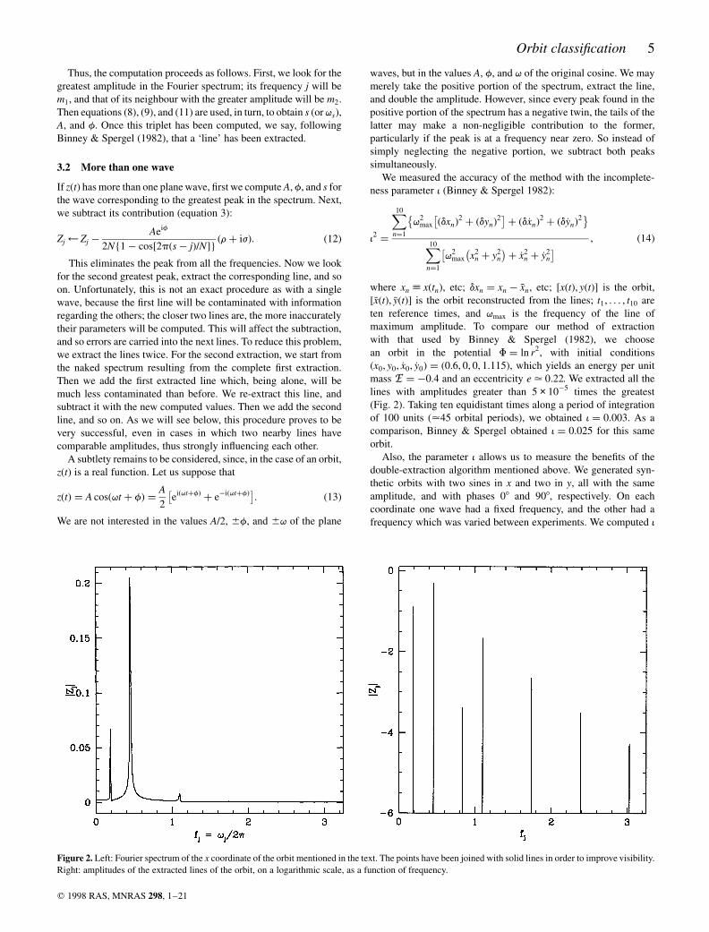
where xn ; xðtnÞ, etc; dxn ¼ xn ¹ xn, etc; ½xðtÞ; yðtÞÿ is the orbit,½xðtÞ; yðtÞÿ is the orbit reconstructed from the lines; t1; . . . ; t10 areten reference times, and qmax is the frequency of the line ofmaximum amplitude. To compare our method of extractionwith that used by Binney & Spergel (1982), we choosean orbit in the potential F ¼ ln r2, with initial conditionsðx0; y0; x0; y0Þ ¼ ð0:6; 0; 0; 1:115Þ, which yields an energy per unitmass E ¼ ¹0:4 and an eccentricity e . 0:22. We extracted all thelines with amplitudes greater than 5 × 10¹5 times the greatest(Fig. 2). Taking ten equidistant times along a period of integrationof 100 units (.45 orbital periods), we obtained i ¼ 0:003. As acomparison, Binney & Spergel obtained i ¼ 0:025 for this sameorbit.

Also, the parameter i allows us to measure the benefits of thedouble-extraction algorithm mentioned above. We generated syn-thetic orbits with two sines in x and two in y, all with the sameamplitude, and with phases 08 and 908, respectively. On eachcoordinate one wave had a fixed frequency, and the other had afrequency which was varied between experiments. We computed i


q 1998 RAS, MNRAS 298, 1–21

Figure 2. Left: Fourier spectrum of the x coordinate of the orbit mentioned in the text. The points have been joined with solid lines in order to improve visibility.Right: amplitudes of the extracted lines of the orbit, on a logarithmic scale, as a function of frequency.

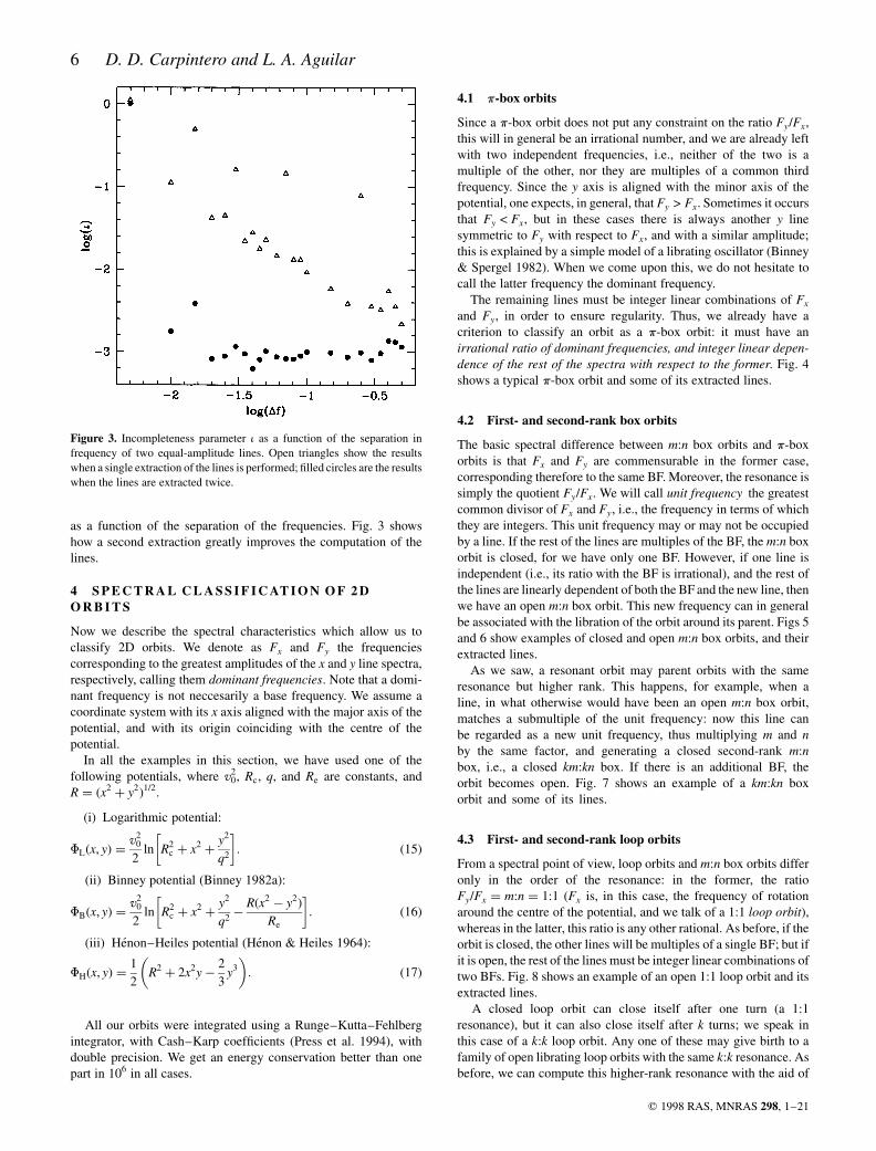
as a function of the separation of the frequencies. Fig. 3 showshow a second extraction greatly improves the computation of thelines.

4 S P E C T R A L C L A S S I F I C AT I O N O F 2 DO R B I T S

Now we describe the spectral characteristics which allow us toclassify 2D orbits. We denote as Fx and Fy the frequenciescorresponding to the greatest amplitudes of the x and y line spectra,respectively, calling them dominant frequencies. Note that a domi-nant frequency is not neccesarily a base frequency. We assume acoordinate system with its x axis aligned with the major axis of thepotential, and with its origin coinciding with the centre of thepotential.

In all the examples in this section, we have used one of thefollowing potentials, where v2

0, Rc, q, and Re are constants, andR ¼ ðx2 þ y2Þ1=2.

(i) Logarithmic potential:

FLðx; yÞ ¼v2

0

2ln R2

c þ x2 þy2

q2

� �: ð15Þ

(ii) Binney potential (Binney 1982a):

FBðx; yÞ ¼v2

0

2ln R2

c þ x2 þy2

q2 ¹Rðx2 ¹ y2Þ

Re

� �: ð16Þ

(iii) Henon–Heiles potential (Henon & Heiles 1964):

FHðx; yÞ ¼12

R2 þ 2x2y ¹23

y3� �

: ð17Þ

All our orbits were integrated using a Runge–Kutta–Fehlbergintegrator, with Cash–Karp coefficients (Press et al. 1994), withdouble precision. We get an energy conservation better than onepart in 106 in all cases.

4.1 p-box orbits

Since a p-box orbit does not put any constraint on the ratio Fy=Fx,this will in general be an irrational number, and we are already leftwith two independent frequencies, i.e., neither of the two is amultiple of the other, nor they are multiples of a common thirdfrequency. Since the y axis is aligned with the minor axis of thepotential, one expects, in general, that Fy > Fx. Sometimes it occursthat Fy < Fx, but in these cases there is always another y linesymmetric to Fy with respect to Fx, and with a similar amplitude;this is explained by a simple model of a librating oscillator (Binney& Spergel 1982). When we come upon this, we do not hesitate tocall the latter frequency the dominant frequency.

The remaining lines must be integer linear combinations of Fx

and Fy, in order to ensure regularity. Thus, we already have acriterion to classify an orbit as a p-box orbit: it must have anirrational ratio of dominant frequencies, and integer linear depen-dence of the rest of the spectra with respect to the former. Fig. 4shows a typical p-box orbit and some of its extracted lines.

4.2 First- and second-rank box orbits

The basic spectral difference between m:n box orbits and p-boxorbits is that Fx and Fy are commensurable in the former case,corresponding therefore to the same BF. Moreover, the resonance issimply the quotient Fy=Fx. We will call unit frequency the greatestcommon divisor of Fx and Fy, i.e., the frequency in terms of whichthey are integers. This unit frequency may or may not be occupiedby a line. If the rest of the lines are multiples of the BF, the m:n boxorbit is closed, for we have only one BF. However, if one line isindependent (i.e., its ratio with the BF is irrational), and the rest ofthe lines are linearly dependent of both the BF and the new line, thenwe have an open m:n box orbit. This new frequency can in generalbe associated with the libration of the orbit around its parent. Figs 5and 6 show examples of closed and open m:n box orbits, and theirextracted lines.

As we saw, a resonant orbit may parent orbits with the sameresonance but higher rank. This happens, for example, when aline, in what otherwise would have been an open m:n box orbit,matches a submultiple of the unit frequency: now this line canbe regarded as a new unit frequency, thus multiplying m and nby the same factor, and generating a closed second-rank m:nbox, i.e., a closed km:kn box. If there is an additional BF, theorbit becomes open. Fig. 7 shows an example of a km:kn boxorbit and some of its lines.

4.3 First- and second-rank loop orbits

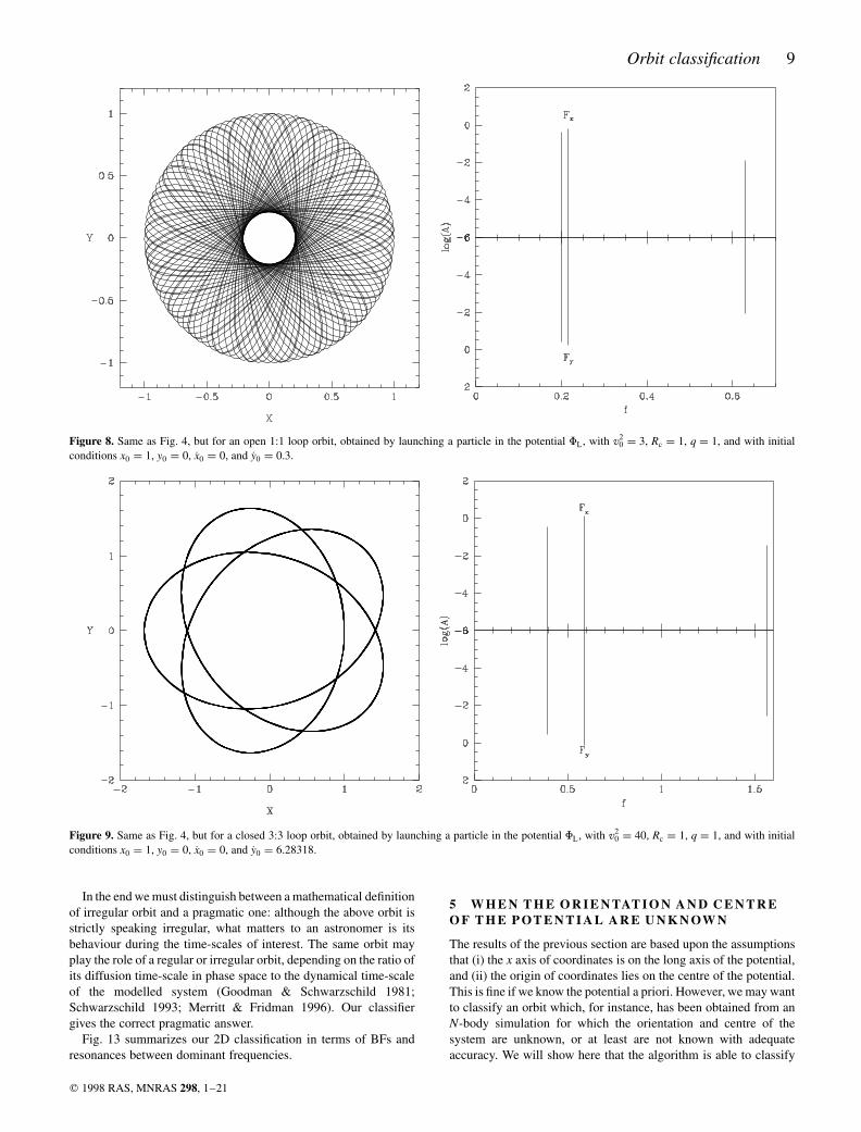
From a spectral point of view, loop orbits and m:n box orbits differonly in the order of the resonance: in the former, the ratioFy=Fx ¼ m:n ¼ 1:1 (Fx is, in this case, the frequency of rotationaround the centre of the potential, and we talk of a 1:1 loop orbit),whereas in the latter, this ratio is any other rational. As before, if theorbit is closed, the other lines will be multiples of a single BF; but ifit is open, the rest of the lines must be integer linear combinations oftwo BFs. Fig. 8 shows an example of an open 1:1 loop orbit and itsextracted lines.

A closed loop orbit can close itself after one turn (a 1:1resonance), but it can also close itself after k turns; we speak inthis case of a k:k loop orbit. Any one of these may give birth to afamily of open librating loop orbits with the same k:k resonance. Asbefore, we can compute this higher-rank resonance with the aid of


q 1998 RAS, MNRAS 298, 1–21

Figure 3. Incompleteness parameter i as a function of the separation infrequency of two equal-amplitude lines. Open triangles show the resultswhen a single extraction of the lines is performed; filled circles are the resultswhen the lines are extracted twice.

the unit frequency. Figs 9 and 10 show examples of a closed 3:3 andan open 2:2 loop orbits, respectively, and their extracted lines.

4.4 Irregular orbits

Since irregular orbits do not have line-like spectra that can beexpressed as integer linear combinations of BFs (in the case of atruly chaotic orbit, even a continuum will appear), the lines

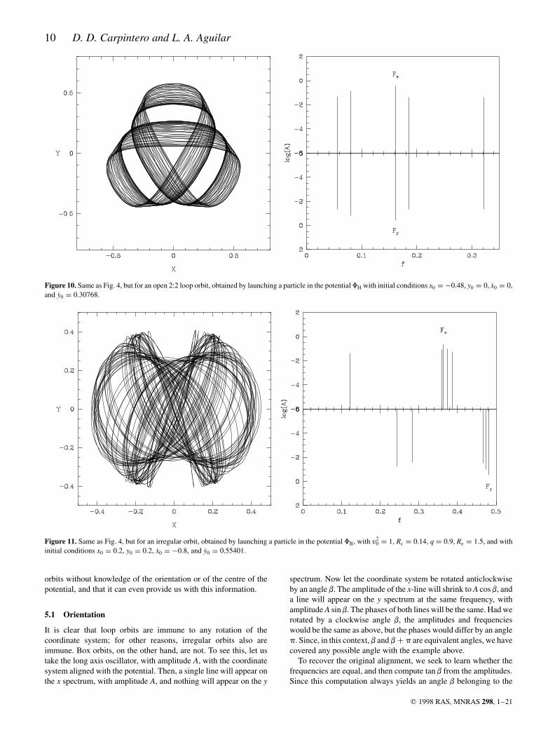
extracted by our algorithm do not describe the orbit, i.e., itsincompleteness parameter i is large. Sometimes, irregular orbitsare close to regular orbits in phase space, and this is reflected in theirspectra; but they always have some extra lines that are not integercombinations of the BFs, which gives them away. Fig. 11 shows anexample of an irregular orbit and its spectra.

A related problem is that of irregular orbits highly confined betweenregular regions, sometimes called ‘sticky’ or ‘semi-stochastic’ orbits


q 1998 RAS, MNRAS 298, 1–21

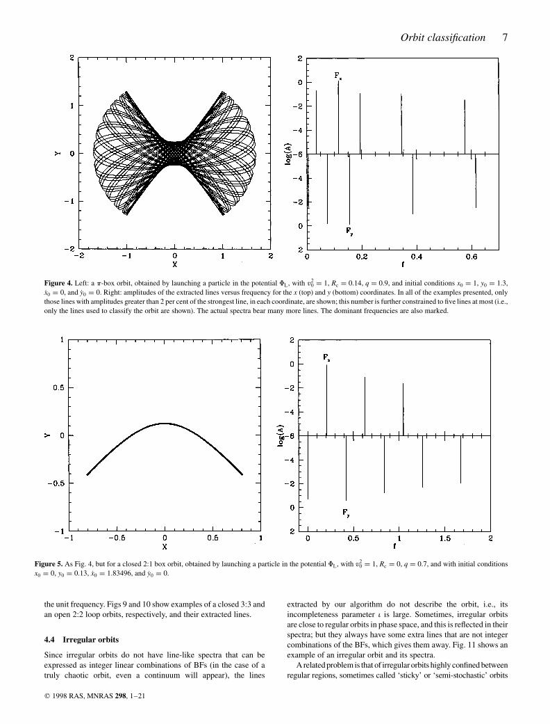
Figure 4. Left: a p-box orbit, obtained by launching a particle in the potential FL, with v20 ¼ 1, Rc ¼ 0:14, q ¼ 0:9, and initial conditions x0 ¼ 1, y0 ¼ 1:3,

x0 ¼ 0, and y0 ¼ 0. Right: amplitudes of the extracted lines versus frequency for the x (top) and y (bottom) coordinates. In all of the examples presented, onlythose lines with amplitudes greater than 2 per cent of the strongest line, in each coordinate, are shown; this number is further constrained to five lines at most (i.e.,only the lines used to classify the orbit are shown). The actual spectra bear many more lines. The dominant frequencies are also marked.

Figure 5. As Fig. 4, but for a closed 2:1 box orbit, obtained by launching a particle in the potential FL, with v20 ¼ 1, Rc ¼ 0, q ¼ 0:7, and with initial conditions

x0 ¼ 0, y0 ¼ 0:13, x0 ¼ 1:83496, and y0 ¼ 0.

(Goodman & Schwarzschild 1981). Such orbits must be givensufficient time to reveal their irregularity without ambiguity, i.e.they need longer integrations to be properly classified. An examplewill illustrate this. Let us launch a particle in the potential FL

with ðv0;Rc; qÞ ¼ ð1; 0; 0:7Þ, and initial conditions ðx0; y0; x0; y0Þ ¼

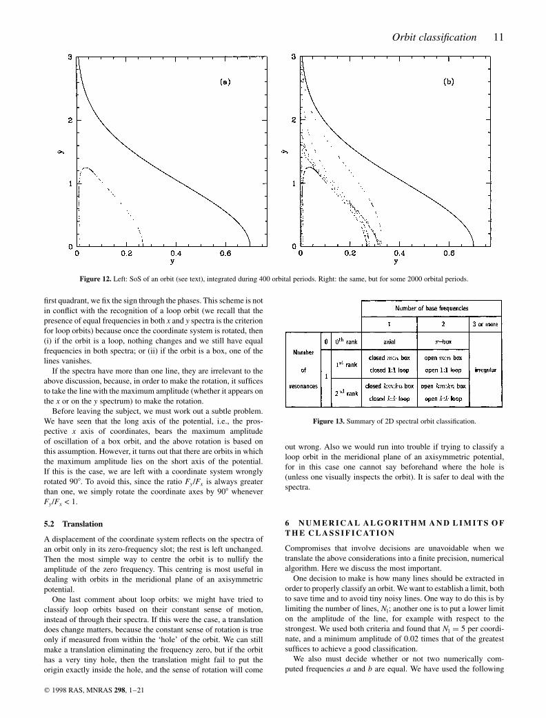
ð0; 0:2663; 1:39029; 0Þ, so that E ¼ 0. This orbit is classified as a 2:1box, but only if we integrate it for fewer than about 400 orbital periods.For longer integrations, our algorithm tells us that it is an irregularorbit. Fig. 12 shows what happens. Fig. 12(a) shows theðy; y; x ¼ 0; x > 0Þ SoS of this orbit, sampled during some 400 orbital

periods. We can see how closely it resembles a regular orbit. Fig. 12(b)shows the same SoS for an integration five times longer. We see thatthe phase space visited has grown, and now we clearly have anirregular orbit. This is just what the algorithm showed. Unfortunately,there is no way to tell in these cases whether or not a furtherintegration period is needed to establish a good classification. Onthe other hand, the orbit has behaved as a regular orbit during the timein which it was classified as such. This orbit was also integrated with adifferent implementation of the Runge–Kutta–Fehlberg integrator(Fehlberg 1968), attaining an energy conservation of one part in 109.


q 1998 RAS, MNRAS 298, 1–21

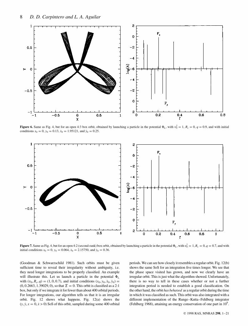
Figure 6. Same as Fig. 4, but for an open 4:3 box orbit, obtained by launching a particle in the potential FL, with v20 ¼ 1, Rc ¼ 0, q ¼ 0:9, and with initial

conditions x0 ¼ 0, y0 ¼ 0:13, x0 ¼ 1:95121, and y0 ¼ 0:25.

Figure 7. Same as Fig. 4, but for an open 4:2 (second-rank) box orbit, obtained by launching a particle in the potential FL, with v20 ¼ 1, Rc ¼ 0, q ¼ 0:7, and with

initial conditions x0 ¼ 0, y0 ¼ 0:064, x0 ¼ 2:15750, and y0 ¼ 0:36.

In the end we must distinguish between a mathematical definitionof irregular orbit and a pragmatic one: although the above orbit isstrictly speaking irregular, what matters to an astronomer is itsbehaviour during the time-scales of interest. The same orbit mayplay the role of a regular or irregular orbit, depending on the ratio ofits diffusion time-scale in phase space to the dynamical time-scaleof the modelled system (Goodman & Schwarzschild 1981;Schwarzschild 1993; Merritt & Fridman 1996). Our classifiergives the correct pragmatic answer.

Fig. 13 summarizes our 2D classification in terms of BFs andresonances between dominant frequencies.

5 W H E N T H E O R I E N TAT I O N A N D C E N T R EO F T H E P OT E N T I A L A R E U N K N OW N

The results of the previous section are based upon the assumptionsthat (i) the x axis of coordinates is on the long axis of the potential,and (ii) the origin of coordinates lies on the centre of the potential.This is fine if we know the potential a priori. However, we may wantto classify an orbit which, for instance, has been obtained from anN-body simulation for which the orientation and centre of thesystem are unknown, or at least are not known with adequateaccuracy. We will show here that the algorithm is able to classify


q 1998 RAS, MNRAS 298, 1–21

Figure 8. Same as Fig. 4, but for an open 1:1 loop orbit, obtained by launching a particle in the potential FL, with v20 ¼ 3, Rc ¼ 1, q ¼ 1, and with initial

conditions x0 ¼ 1, y0 ¼ 0, x0 ¼ 0, and y0 ¼ 0:3.

Figure 9. Same as Fig. 4, but for a closed 3:3 loop orbit, obtained by launching a particle in the potential FL, with v20 ¼ 40, Rc ¼ 1, q ¼ 1, and with initial

conditions x0 ¼ 1, y0 ¼ 0, x0 ¼ 0, and y0 ¼ 6:28318.

orbits without knowledge of the orientation or of the centre of thepotential, and that it can even provide us with this information.

5.1 Orientation

It is clear that loop orbits are immune to any rotation of thecoordinate system; for other reasons, irregular orbits also areimmune. Box orbits, on the other hand, are not. To see this, let ustake the long axis oscillator, with amplitude A, with the coordinatesystem aligned with the potential. Then, a single line will appear onthe x spectrum, with amplitude A, and nothing will appear on the y

spectrum. Now let the coordinate system be rotated anticlockwiseby an angle b. The amplitude of the x-line will shrink to A cos b, anda line will appear on the y spectrum at the same frequency, withamplitude A sin b. The phases of both lines will be the same. Had werotated by a clockwise angle b, the amplitudes and frequencieswould be the same as above, but the phases would differ by an anglep. Since, in this context, b and b þ p are equivalent angles, we havecovered any possible angle with the example above.

To recover the original alignment, we seek to learn whether thefrequencies are equal, and then compute tan b from the amplitudes.Since this computation always yields an angle b belonging to the


q 1998 RAS, MNRAS 298, 1–21

Figure 10. Same as Fig. 4, but for an open 2:2 loop orbit, obtained by launching a particle in the potential FH with initial conditions x0 ¼ ¹0:48, y0 ¼ 0, x0 ¼ 0,and y0 ¼ 0:30768.

Figure 11. Same as Fig. 4, but for an irregular orbit, obtained by launching a particle in the potential FB, with v20 ¼ 1, Rc ¼ 0:14, q ¼ 0:9, Re ¼ 1:5, and with

initial conditions x0 ¼ 0:2, y0 ¼ 0:2, x0 ¼ ¹0:8, and y0 ¼ 0:55401.

first quadrant, we fix the sign through the phases. This scheme is notin conflict with the recognition of a loop orbit (we recall that thepresence of equal frequencies in both x and y spectra is the criterionfor loop orbits) because once the coordinate system is rotated, then(i) if the orbit is a loop, nothing changes and we still have equalfrequencies in both spectra; or (ii) if the orbit is a box, one of thelines vanishes.

If the spectra have more than one line, they are irrelevant to theabove discussion, because, in order to make the rotation, it sufficesto take the line with the maximum amplitude (whether it appears onthe x or on the y spectrum) to make the rotation.

Before leaving the subject, we must work out a subtle problem.We have seen that the long axis of the potential, i.e., the pros-pective x axis of coordinates, bears the maximum amplitudeof oscillation of a box orbit, and the above rotation is based onthis assumption. However, it turns out that there are orbits in whichthe maximum amplitude lies on the short axis of the potential.If this is the case, we are left with a coordinate system wronglyrotated 908. To avoid this, since the ratio Fy=Fx is always greaterthan one, we simply rotate the coordinate axes by 908 wheneverFy=Fx < 1.

5.2 Translation

A displacement of the coordinate system reflects on the spectra ofan orbit only in its zero-frequency slot; the rest is left unchanged.Then the most simple way to centre the orbit is to nullify theamplitude of the zero frequency. This centring is most useful indealing with orbits in the meridional plane of an axisymmetricpotential.

One last comment about loop orbits: we might have tried toclassify loop orbits based on their constant sense of motion,instead of through their spectra. If this were the case, a translationdoes change matters, because the constant sense of rotation is trueonly if measured from within the ‘hole’ of the orbit. We can stillmake a translation eliminating the frequency zero, but if the orbithas a very tiny hole, then the translation might fail to put theorigin exactly inside the hole, and the sense of rotation will come

out wrong. Also we would run into trouble if trying to classify aloop orbit in the meridional plane of an axisymmetric potential,for in this case one cannot say beforehand where the hole is(unless one visually inspects the orbit). It is safer to deal with thespectra.

6 N U M E R I C A L A L G O R I T H M A N D L I M I T S O FT H E C L A S S I F I C AT I O N

Compromises that involve decisions are unavoidable when wetranslate the above considerations into a finite precision, numericalalgorithm. Here we discuss the most important.

One decision to make is how many lines should be extracted inorder to properly classify an orbit. We want to establish a limit, bothto save time and to avoid tiny noisy lines. One way to do this is bylimiting the number of lines, Nl; another one is to put a lower limiton the amplitude of the line, for example with respect to thestrongest. We used both criteria and found that Nl ¼ 5 per coordi-nate, and a minimum amplitude of 0.02 times that of the greatestsuffices to achieve a good classification.

We also must decide whether or not two numerically com-puted frequencies a and b are equal. We have used the following


q 1998 RAS, MNRAS 298, 1–21

Figure 12. Left: SoS of an orbit (see text), integrated during 400 orbital periods. Right: the same, but for some 2000 orbital periods.

Figure 13. Summary of 2D spectral orbit classification.

criterion,

a ¼ b ⇔ ja ¹ bj

jaj þ 1< « D; ð18Þ

where D is the difference in frequency between two adjacentFourier slots, and « is a parameter to fix. We found that « . 0:25is a good compromise.

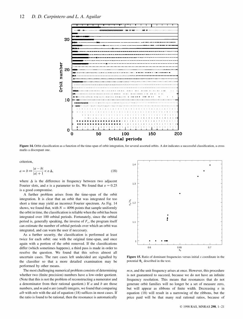
A further problem arises from the time-span of the orbitintegration. It is clear that an orbit that was integrated for tooshort a time may yield an incorrect Fourier spectrum. As Fig. 14shows, we found that, with N ¼ 4096 points that sample uniformlythe orbit in time, the classification is reliable when the orbit has beenintegrated over 100 orbital periods. Fortunately, since the orbitalperiod is, generally speaking, the inverse of Fx, the program itselfcan estimate the number of orbital periods over which an orbit wasintegrated, and can warn the user if neccesary.

As a further security, the classification is performed at leasttwice for each orbit: one with the original time-span, and onceagain with a portion of the orbit removed. If the classificationsdiffer (which sometimes happens), a third pass is made in order toresolve the question. We found that this solves almost alluncertain cases. The rare cases left undecided are signalled bythe classifier so that a more detailed examination may beperformed by other means.

The most challenging numerical problem consists of determiningwhether two (finite precision) numbers have a low-order quotient.(Note that this is not the problem of reconstructing a numerator anda denominator from their rational quotient.) If a and b are thosenumbers, and m and n are (small) integers, we found that comparinga=b with m=n with the aid of equation (18) suffices in most cases. Ifthe ratio is found to be rational, then the resonance is automatically

m:n, and the unit frequency arises at once. However, this procedureis not guaranteed to succeed, because we do not have an infinitefrequency resolution. This means that resonances that do notgenerate orbit families will no longer be a set of measure zero,but will appear as ribbons of finite width. Decreasing « inequation (18) will result in a narrowing of the ribbons, but theprice paid will be that many real rational ratios, because of


q 1998 RAS, MNRAS 298, 1–21

Figure 14. Orbit classification as a function of the time-span of orbit integration, for several assorted orbits. A dot indicates a successful classification, a crossmarks a discrepant one.

0.6 0.65 0.7

1

1.1

1.2

1.3

1.4

Figure 15. Ratio of dominant frequencies versus initial x coordinate in thepotential FL described in the text.


q 1998 RAS, MNRAS 298, 1–21

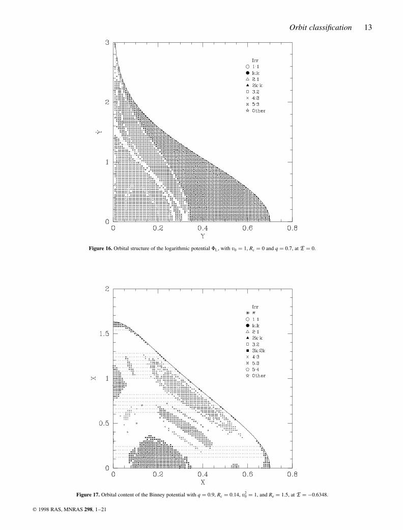
Figure 16. Orbital structure of the logarithmic potential FL, with v0 ¼ 1, Rc ¼ 0 and q ¼ 0:7, at E ¼ 0.

Figure 17. Orbital content of the Binney potential with q ¼ 0:9, Rc ¼ 0:14, v20 ¼ 1, and Re ¼ 1:5, at E ¼ ¹0:6348.

inaccuracies in the determination of their frequencies, will beconsidered irrational, thus resulting in spurious irregular orbits. Inthe end, one must recognize that any numerical tool will have limitsin resolution.

However, the classifier is still a powerful tool. We integrated aseries of orbits in the potential FL with v0 ¼ 1, q ¼ 0:9, andRc ¼ 0:14, at an energy E ¼ ¹0:337 (BT87, fig. 3.8), with initialconditions 0:6 # x0 # 0:7, x0 ¼ y0 ¼ 0, and y0 chosen to match theenergy. Thus, this series crosses from the loop to the box region ofthe potential. Fig. 15 shows the ratio of dominant frequencies alongthis series. The classifier sharply recognizes the border betweenfamilies (qy=qx ¼ 1 for loops, > 1 for p-boxes). The first two orbits,from left to right, with ratios > 1, were classified as irregulars. Therest were classified as loops (left) or p-boxes (right).

7 R E S U LT S F O R 2 D P OT E N T I A L S

To test our classifier, we analysed the orbital structure of severalpotentials previously studied, so that we could compare the results.

Fig. 16 shows a grid of orbits that we have classified on the SoSfor the logarithmic potential FL, with q ¼ 0:7, Rc ¼ 0, v2

0 ¼ 1, thatcorresponds to an energy per unit mass E ¼ 0 (in this and otherexamples in this section, every symbol in the corresponding figurerepresents the initial point of an orbit that was integrated andclassified separately). This is to be compared with fig. 1 ofMiralda-Escude & Schwarzschild (1989). As indicated by theseauthors, there is a complete lack of p-box orbits, and irregular orbitsfill the phase space between the different classes of regular orbits.All resonances found by these authors have been found by ourclassifier, and, at the higher resolution of our grid, further fine detailis beginning to appear. Resonances as high as 8:5 appear close to

y , 0 and y < 1:4 (labelled as ‘other’ in the figure), narrow strips ofk:k loops at the border and within the region occupied by the open1:1 loops orbits, and also narrow strips of 2k:k boxes within theregion of 2:1 boxes. The ‘irregular sea’ in this SoS appears to be allconnected as can be seen in Fig. 12(b), which shows an irregularorbit that loiters around almost all of the irregular bands betweenregular zones in this SoS. The few irregulars close to the 2k:k orbits,when inspected, reveal themselves as 4:2 boxes, so we are here atthe limit of frequency resolution of the classifier.

Fig. 17 shows a similar SoS grid, but for the Binney potentialFB, with q ¼ 0:9, Rc ¼ 0:14, v2

0 ¼ 1, and Re ¼ 1:5, atE ¼ ¹0:6348. As can be seen, there are islands of regularorbits in a sea of irregularity. Again, second-rank resonanceorbits begin to show up. This figure can be compared with figs3–27 of BT87, where some orbits were sketched. Our classifiercombined with a finer grid gives us a higher resolution picture ofthe orbital structure of this particular SoS.

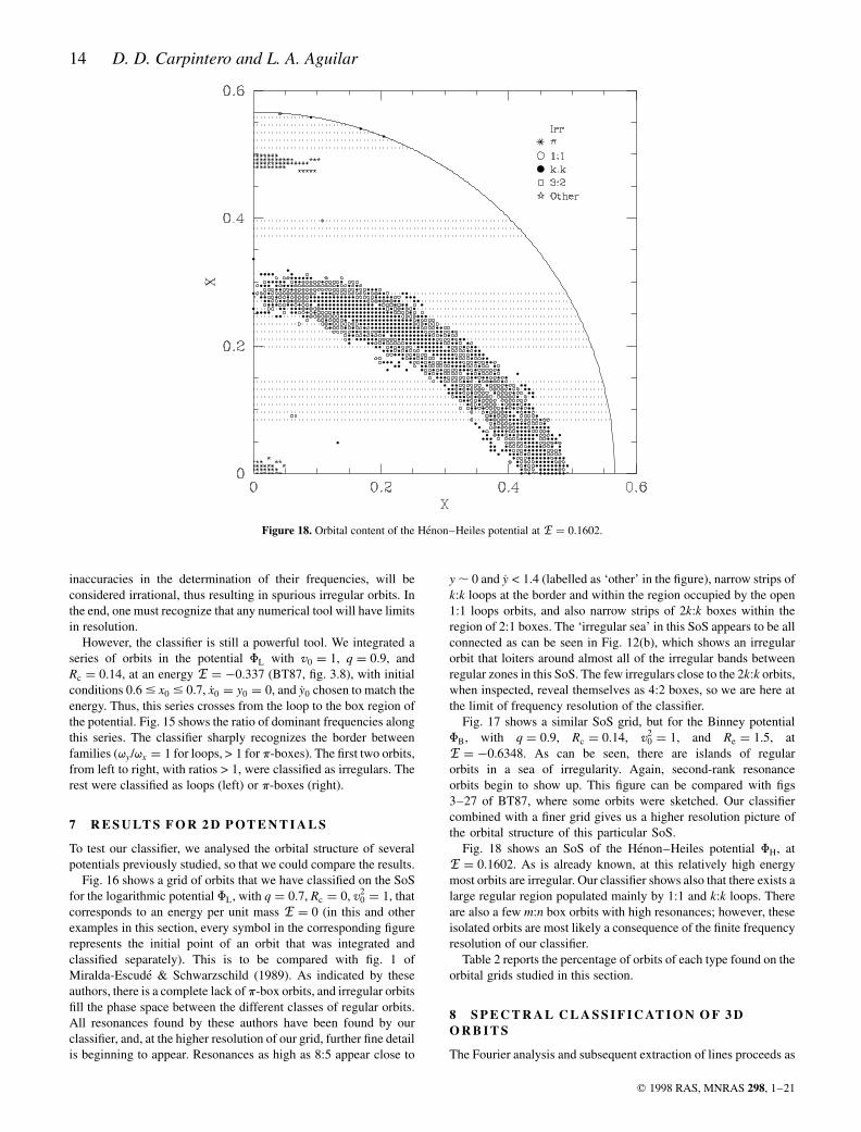
Fig. 18 shows an SoS of the Henon–Heiles potential FH, atE ¼ 0:1602. As is already known, at this relatively high energymost orbits are irregular. Our classifier shows also that there exists alarge regular region populated mainly by 1:1 and k:k loops. Thereare also a few m:n box orbits with high resonances; however, theseisolated orbits are most likely a consequence of the finite frequencyresolution of our classifier.

Table 2 reports the percentage of orbits of each type found on theorbital grids studied in this section.

8 S P E C T R A L C L A S S I F I C AT I O N O F 3 DO R B I T S

The Fourier analysis and subsequent extraction of lines proceeds as


q 1998 RAS, MNRAS 298, 1–21

Figure 18. Orbital content of the Henon–Heiles potential at E ¼ 0:1602.

in 2D. The only change is in the classification itself. We assume thatthe x, y, and z axes correspond to the large, intermediate, and shortaxes of the potential, respectively. First, we determine the dominantfrequencies in each coordinate, denoting them Fx, Fy, and Fz.

Now we take each couple of coordinates ðx; yÞ, ðx; zÞ, ðy; zÞ in turn.For each case, we analyse whether the second-dominant line mustbear the title of dominant, as we explained in Section 4.1. Then,again for each pair, we compute whether or not they have a rationalratio, i.e., whether a resonance is present. If this is the case, wecompute the integer numerator and denominator, as described inSection 6. In each case, we search for the possibility of an improperquotient related to a higher-rank resonance, and compute numera-tors and denominators accordingly. Once the three pairs of coordi-nates have been surveyed, we are left with zero, one, two or threeresonances encountered.

If we find three resonances, i.e., one resonance in each pair ofcoordinates, then all three dominant frequencies are multiples of asingle unit frequency. We then build the relationship between thethree coordinates in the form of a proportion among integers X:Y:Z,taking into account any present higher-rank resonance.

When the program finds only two resonances (which is, ofcourse, not possible), what happens is that one of the quotients islikely to be formed by two large integers beyond the range searchedby the classifier. We then reconstruct the lost resonance from theother two, ensuring that no spurious improper resonances leak in.

If we find only one resonance, say Y=X, then it means that Fz hasan irrational relation with respect to Fx and Fy. In this case, we willdenote the irrational ratios by putting Z ¼ p, thus yielding thetriplet X:Y:p. Of course, the same holds if Z=X or Z=Y were the case.

If no resonances are encountered, all three dominant frequenciesare irrationally related. This corresponds to the 3D analogues of the2D p-boxes. Extending our foregoing notation, we will call them3D p-boxes.

We can now establish the number of BFs among the dominantfrequencies: if there are three resonances, there is one BF; if there isone resonance, there are two BFs; and if no resonances were foundat all, there are three BFs. With these figures, we go on searching foradditional BFs, i.e., frequencies present in the orbit but that are notinteger linear combinations of the dominant-born BFs. The proce-dure goes much as in the 2D case, but now we make room for up tofour possible independent frequencies.

The last step is to classify the orbit from the data collected above.First, we consider the total number of BFs: if we find a total of more

than three BFs, the orbit is irregular and the BFs are not really BFs.If fewer than four BFs are found, we have regular orbits that areclosed (one BF) or open (three BFs). If there are two BFs, the orbitmoves on a 2D manifold in configuration space. Following the usualnomenclature, we will call these orbits thin.

Secondly, we consider the number of resonances. When there areno resonances, then the orbit is an axial orbit (one BF), a 2D p-box(two BFs) or a 3D p-box (three BFs). If there is one resonance, wehave a 2D closed box (one BF), a thin box (two BFs) or an open box(three BFs); except when the resonance is 1:1, in which case wehave closed loops, thin tubes and open tubes, respectively. Finally,the orbits whose dominant frequencies are all in resonance, andwith three or two BFs, are boxes or tubes the parents of which arethe corresponding 3D closed resonant orbits with one BF.

The particular case of a 1:1 resonance between two coordinatesgives rise to the familiar z-tubes, if x and y are resonant, or x-tubes, ify and z are resonant. (In rare cases, as in a fully harmonic 3Dpotential, we may also have y-tubes or two or three k:k relations).Although we were not able to find any distinguishing featurebetween so-called outer x-tubes and inner x-tubes (de Zeeuw1985) spectra, we can fill this gap with a simple routine, computingfrom the coordinates of the orbit whether it is concave (outer x-tube)or convex (inner x-tube) in the x direction. However, it turned outthat this routine could not handle all the cases properly, as some-times the curvature was subtle. A better routine remains to becreated.

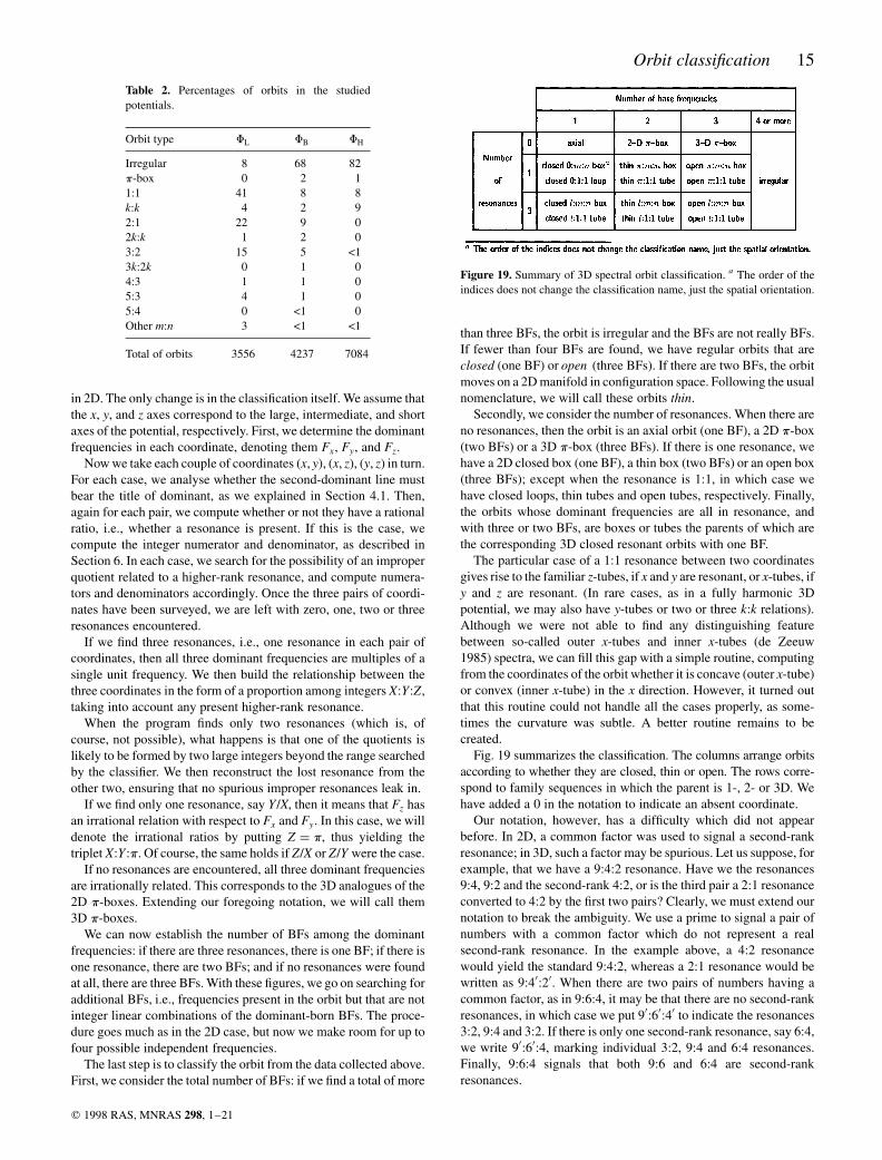
Fig. 19 summarizes the classification. The columns arrange orbitsaccording to whether they are closed, thin or open. The rows corre-spond to family sequences in which the parent is 1-, 2- or 3D. Wehave added a 0 in the notation to indicate an absent coordinate.

Our notation, however, has a difficulty which did not appearbefore. In 2D, a common factor was used to signal a second-rankresonance; in 3D, such a factor may be spurious. Let us suppose, forexample, that we have a 9:4:2 resonance. Have we the resonances9:4, 9:2 and the second-rank 4:2, or is the third pair a 2:1 resonanceconverted to 4:2 by the first two pairs? Clearly, we must extend ournotation to break the ambiguity. We use a prime to signal a pair ofnumbers with a common factor which do not represent a realsecond-rank resonance. In the example above, a 4:2 resonancewould yield the standard 9:4:2, whereas a 2:1 resonance would bewritten as 9:40:20. When there are two pairs of numbers having acommon factor, as in 9:6:4, it may be that there are no second-rankresonances, in which case we put 90:60:40 to indicate the resonances3:2, 9:4 and 3:2. If there is only one second-rank resonance, say 6:4,we write 90:60:4, marking individual 3:2, 9:4 and 6:4 resonances.Finally, 9:6:4 signals that both 9:6 and 6:4 are second-rankresonances.


q 1998 RAS, MNRAS 298, 1–21

Table 2. Percentages of orbits in the studiedpotentials.

Orbit type FL FB FH

Irregular 8 68 82p-box 0 2 11:1 41 8 8k:k 4 2 92:1 22 9 02k:k 1 2 03:2 15 5 <13k:2k 0 1 04:3 1 1 05:3 4 1 05:4 0 <1 0Other m:n 3 <1 <1

Total of orbits 3556 4237 7084

Figure 19. Summary of 3D spectral orbit classification. a The order of theindices does not change the classification name, just the spatial orientation.

As in the 2D case, we perform a second classification byremoving a portion of the orbit; if the classification differs, a thirdpass is made with another orbital portion removed.

The position of the centre of the 3D potential is obtained bymeans of a simple extrapolation of the method described in 2D. Theorientation, on the other hand, is far from this simple. We have notyet developed the corresponding algorithm.

9 R E S U LT S F O R 3 D P OT E N T I A L S

As for the 2D case, we study some potentials the orbital structure ofwhich is either simple, or has been determined independently, to testthe validity of our classifier.

We first tested the classifier with orbits in a 3D harmonicoscillator, obtaining good classifications in all cases.

A non-trivial and fully regular and well-studied potential is the‘perfect ellipsoid’ (de Zeeuw 1985; BT87), a member of the familyof Stackel potentials (Stackel 1890). Although it has its simplerform in ellipsoidal coordinates, which is not very convenient fornumerical integration, we have used this potential because it has themajor four families of 3D orbits, and by computing the threeintegrals of motion, one can know a priori which type of orbitone is working with, and then confront this result with the output ofour classifier.

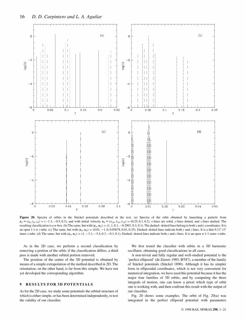
Fig. 20 shows some examples. The orbit of Fig. 20(a) wasintegrated in the perfect ellipsoid potential with parameters


q 1998 RAS, MNRAS 298, 1–21

(d)

Figure 20. Spectra of orbits in the Stackel potentials described in the text. (a) Spectra of the orbit obtained by launching a particle fromx0 ; ðx0; y0; z0Þ ¼ ð¹1:3;¹0:5; 0:3Þ, and with initial velocity v0 ; ðvx0; vy0; vz0Þ ¼ ð0:25; 0:1; 0:2Þ. x-lines are solid, y-lines dotted, and z-lines dashed. Theresulting classification is a p-box. (b) The same, but with ðx0;v0Þ ¼ ð1; 1; 0:1;¹0:2901; 0:3; 0:1Þ. The dashed–dotted lines belong to both x and y coordinates. It isan open 1:1:p z-tube. (c) The same, but with ðx0;v0Þ ¼ ð0:01;¹1; 0; 0:05678; 0:01; 0:35Þ. Dashed–dotted lines indicate both y and z lines. It is a thin 9:130:130

inner x-tube. (d) The same, but with ðx0;v0Þ ¼ ð1; ¹3:1;¹5:4; 0:3;¹0:1; 0:1Þ. Dashed–dotted lines indicate both y and z lines. It is an open p:1:1 outer x-tube.

a ¼ ¹1, b ¼ ¹0:390 625, and g ¼ ¹0:25. It is a 3D p-box; lines ofeach coordinate are marked with different line types. Note how eachpair of coordinates makes a 2D p-box spectrum on its own. Fig.20(b) shows the spectra of an open 1:1:p tube (a z-tube), integratedin the same potential with parameters a ¼ ¹2, b ¼ ¹1, andg ¼ ¹0:5; in this case, the lines belonging to the x and y coordinateshave the same frequencies, and so the amplitude shown is only thegreatest among x and y. Fig. 20(c) shows an example of a thin innerx-tube, integrated in the prolate limit of the perfect ellipsoidpotential (de Zeeuw 1985) with parameters a ¼ ¹4 and b ¼ ¹1;here the frequencies of the y- and z-lines are the same. Fig. 20(d)shows the spectra of a p:1:1 outer x-tube, integrated in the samepotential of Fig. 20(a).

Schwarzschild (1993) has investigated the possibility of self-consistent models in a singular, triaxial logarithmic potential,expanded in spherical harmonics. We have used this referencebecause the orbital classification for 3600 orbits on six variants ofthis potential in two so-called ‘start spaces’ is given, and the preciseresonance is listed for 64 stable, closed orbits, together with theirinitial conditions (tables 3 and 4 of Schwarzschild 1993). Theseorbits span a rich variety of resonances as high as 31:42:51. Theclassification accomplished in this work represents a tour de force,achieved by considering the symmetry and behaviour of the meanangular momenta and positions along each axis, as well as thecorresponding extrema. The way in which the precise resonanceorder has been found is through a visual inspection of the plots ofthe individual time series for each coordinate (Schwarzschild,private communication), a daunting task indeed, when consideringthe high order of some resonances.

We have integrated all stable closed orbits listed in this work for80 periods. We were pleased to see that for all but 4 of the 64 orbits,we obtained the same classification as Schwarzschild, including theresonance, the closeness, and all the second-rank resonances, whichSchwarzschild calls ‘higher period multiples’. Here follows anaccount of the discrepant cases.

(i) In table 3 of the above reference, we found that orbit number3 of the C ¼ 0:7, T ¼ 0:5 model, and orbit number 3 of the C ¼ 0:3,T ¼ 0:5 model, were thin 1:p:2 boxes, i.e. there were two BFs, andtherefore they were not closed. The classification given bySchwarzschild is 1:S:2. We note that a letter ‘S’ appears in histables 3 and 4 whenever there is no motion on a coordinate, excepton these two cases where, according to us, it should indicate a non-resonant coordinate; interestingly enough, an S is used to indicateprecisely this on his table 1.

(ii) In his table 4, orbit number 7 of the C ¼ 0:7, T ¼ 0:5 modelwas found to be a p:42:51 box, instead of a 31:42:51 box. That is,our program found two irrational quotients instead of the relations31:42 and 31:51, and a 14:17 resonance which turned out to beimproper, becoming the 42:51 quotient. We can tune the algorithmin order to detect even these high quotients (we did it and found theright classification); this practice, however, may render the algo-rithm unable to find irrational quotients (see Section 6). We prefer tostick with a ‘safe’ algorithm, losing high resonances, which are notvery important.

(iii) In table 4 of Schwarzschild (1993), orbit number 3 of theC ¼ 0:3, T ¼ 0:98 model was found to be a 2:3:0 box (a planarfish), instead of a reported 2:3:5. This is clearly a mere misprint inthe reference, which must then read 2:3:S.

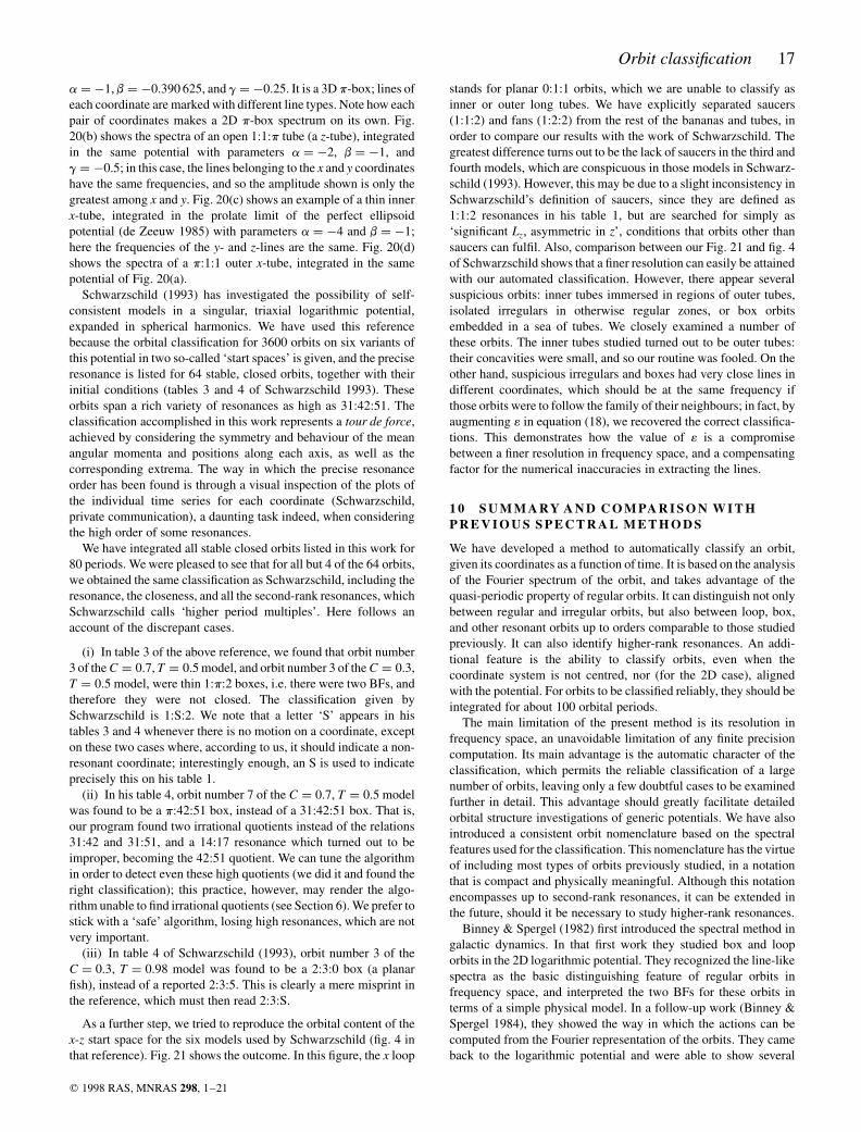
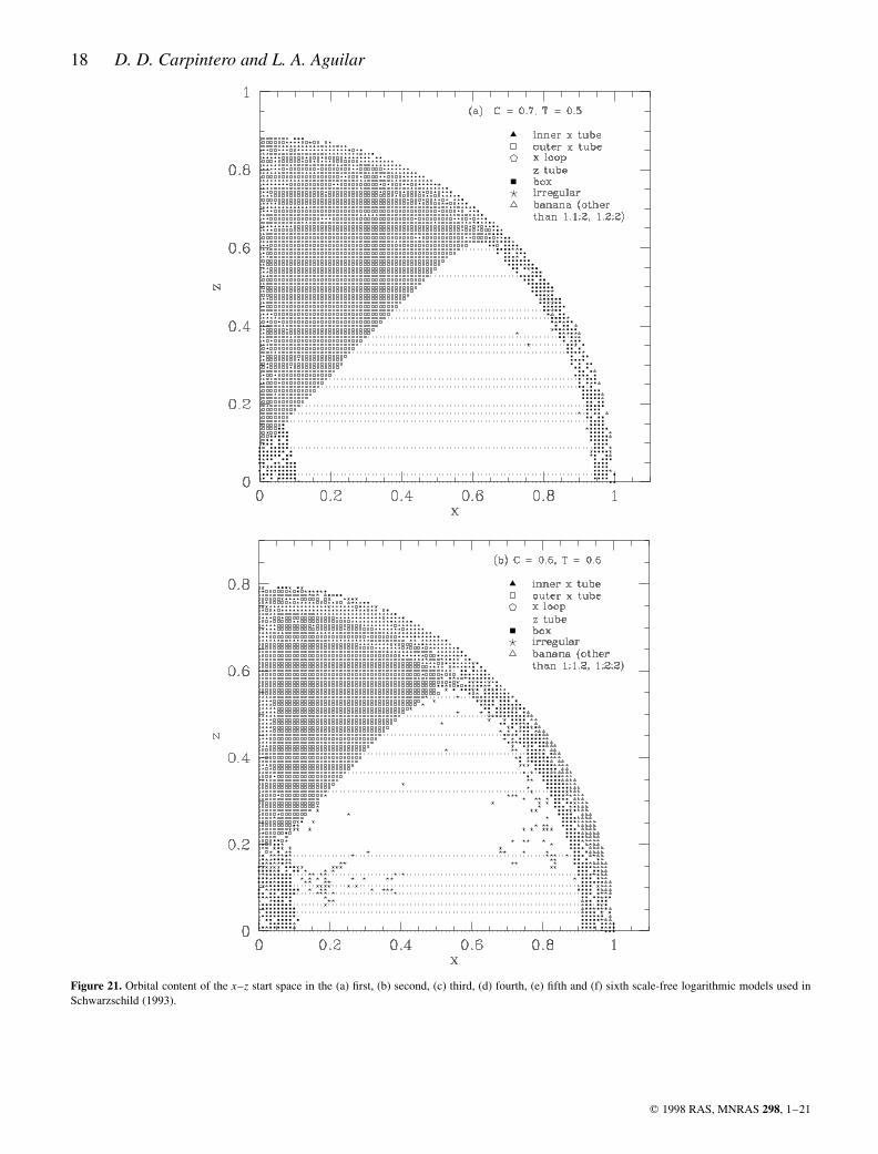
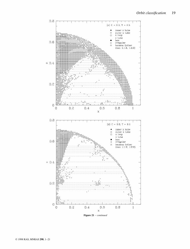
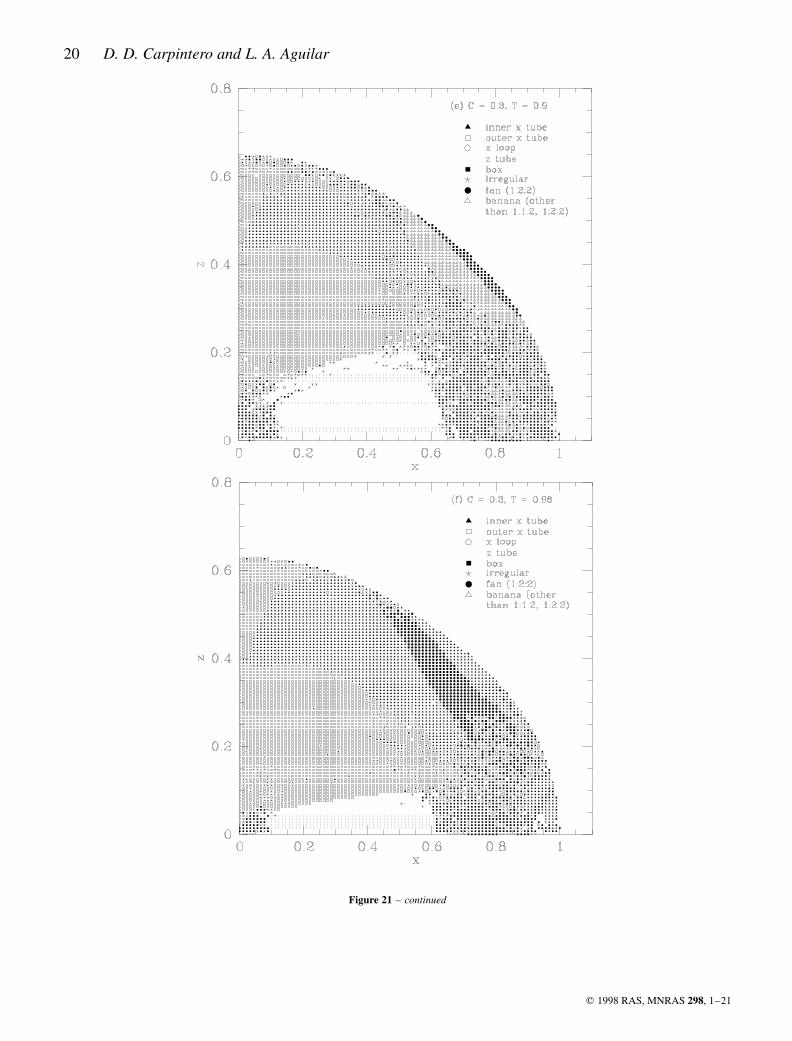
As a further step, we tried to reproduce the orbital content of thex-z start space for the six models used by Schwarzschild (fig. 4 inthat reference). Fig. 21 shows the outcome. In this figure, the x loop

stands for planar 0:1:1 orbits, which we are unable to classify asinner or outer long tubes. We have explicitly separated saucers(1:1:2) and fans (1:2:2) from the rest of the bananas and tubes, inorder to compare our results with the work of Schwarzschild. Thegreatest difference turns out to be the lack of saucers in the third andfourth models, which are conspicuous in those models in Schwarz-schild (1993). However, this may be due to a slight inconsistency inSchwarzschild’s definition of saucers, since they are defined as1:1:2 resonances in his table 1, but are searched for simply as‘significant Lz, asymmetric in z’, conditions that orbits other thansaucers can fulfil. Also, comparison between our Fig. 21 and fig. 4of Schwarzschild shows that a finer resolution can easily be attainedwith our automated classification. However, there appear severalsuspicious orbits: inner tubes immersed in regions of outer tubes,isolated irregulars in otherwise regular zones, or box orbitsembedded in a sea of tubes. We closely examined a number ofthese orbits. The inner tubes studied turned out to be outer tubes:their concavities were small, and so our routine was fooled. On theother hand, suspicious irregulars and boxes had very close lines indifferent coordinates, which should be at the same frequency ifthose orbits were to follow the family of their neighbours; in fact, byaugmenting « in equation (18), we recovered the correct classifica-tions. This demonstrates how the value of « is a compromisebetween a finer resolution in frequency space, and a compensatingfactor for the numerical inaccuracies in extracting the lines.

1 0 S U M M A RY A N D C O M PA R I S O N W I T HP R E V I O U S S P E C T R A L M E T H O D S

We have developed a method to automatically classify an orbit,given its coordinates as a function of time. It is based on the analysisof the Fourier spectrum of the orbit, and takes advantage of thequasi-periodic property of regular orbits. It can distinguish not onlybetween regular and irregular orbits, but also between loop, box,and other resonant orbits up to orders comparable to those studiedpreviously. It can also identify higher-rank resonances. An addi-tional feature is the ability to classify orbits, even when thecoordinate system is not centred, nor (for the 2D case), alignedwith the potential. For orbits to be classified reliably, they should beintegrated for about 100 orbital periods.

The main limitation of the present method is its resolution infrequency space, an unavoidable limitation of any finite precisioncomputation. Its main advantage is the automatic character of theclassification, which permits the reliable classification of a largenumber of orbits, leaving only a few doubtful cases to be examinedfurther in detail. This advantage should greatly facilitate detailedorbital structure investigations of generic potentials. We have alsointroduced a consistent orbit nomenclature based on the spectralfeatures used for the classification. This nomenclature has the virtueof including most types of orbits previously studied, in a notationthat is compact and physically meaningful. Although this notationencompasses up to second-rank resonances, it can be extended inthe future, should it be necessary to study higher-rank resonances.

Binney & Spergel (1982) first introduced the spectral method ingalactic dynamics. In that first work they studied box and looporbits in the 2D logarithmic potential. They recognized the line-likespectra as the basic distinguishing feature of regular orbits infrequency space, and interpreted the two BFs for these orbits interms of a simple physical model. In a follow-up work (Binney &Spergel 1984), they showed the way in which the actions can becomputed from the Fourier representation of the orbits. They cameback to the logarithmic potential and were able to show several


q 1998 RAS, MNRAS 298, 1–21


q 1998 RAS, MNRAS 298, 1–21

Figure 21. Orbital content of the x–z start space in the (a) first, (b) second, (c) third, (d) fourth, (e) fifth and (f) sixth scale-free logarithmic models used inSchwarzschild (1993).


q 1998 RAS, MNRAS 298, 1–21

Figure 21 – continued

important results, e.g. the way in which regular orbit families fit inaction space.

More recently, Laskar (1993) has reintroduced the spectralmethod within the context of stability studies of orbits in conserva-tive dynamical systems. Laskar obtains the BFs using phase-spacecoordinates in an iterative numerical algorithm that results in a veryaccurate determination of frequencies and phases. Papaphilippou &Laskar (1996) have used this method to study the same logarithmicpotential studied by Binney & Spergel. The actions of box and looporbits are then approximated by means of the spectral representa-tion. The main thrust of this work is the study of the orbital structureby means of a 1D map from one phase-space variable to frequencyspace. Resonances as high as 9:16 are identified by means of thistechnique.

Our approach has been different, as our main goal has been to getan automatic orbit classifier. Our procedure for extracting lines isbetter than the one originally used by Binney & Spergel, but doesnot seem to be as good as the one claimed by Laskar. Our precision,however, seems to be adequate to obtain the desired classification.The identification of the particular behaviour of line frequencies inFourier space, which we use to accomplish the classification, wasnot contemplated in those earlier references.

In computing the BFs for an orbit, we are obtaining the basicfrequencies that occur in action–angle theory. This being ofimportance itself, further work remains to be done; in particular,the computation of the action integrals for 3D orbits extending themethod introduced by Binney & Spergel (1984) is of paramountimportance, because they provide a natural coordinate system onwhich to study the phase-space distribution of regular dynamicalsystems. Another interesting line of work would be to investigatewhether chaotic orbits can be identified by means of the continuumthey produce in Fourier space. We hope to pursue these lines ofinvestigation in the future.

The program developed to accomplish the orbit classification isavailable for general use upon request.

AC K N OW L E D G M E N T S

We thank R. Montgomery and F. Fasso for illuminating discussionson the intrincancies of non-linear dynamics, and M. Aragon forproviding us with a useful algorithm. We are also indebted to T. deZeeuw, J. Binney, D. Merritt, and M. Schwarzschild, who read themanuscript and made valuable comments. M. Schwarzschild, inparticular, made a very thorough examination that resulted in newinsights into the problem. L. Aguilar acknowledges the hospitalityof the Leiden Observatory, where part of this work was written. Hisstay there was supported in part by a Bezoerersbeurs from NWO(the Netherlands Foundation for Scientific Research), and in part byDGAPA (the National University of Mexico). D. Carpintero acknow-ledges Commision 38 of the I.A.U. for providing funds to travel toMexico. This work was supported by CONACYT grant 3739-E.

R E F E R E N C E S

Arnold V. I., 1989, Mathematical Methods of Classical Mechanics.Springer-Verlag, New York

Binney J., 1982a, MNRAS, 201, 1Binney J., 1982b, MNRAS, 201, 15Binney J., Spergel D., 1982, ApJ, 252, 308Binney J., Spergel D., 1984, MNRAS, 206, 159Binney J., Tremaine S., 1987, Galactic Dynamics. Princeton Univ. Press,

Princeton NJ (BT87)Contopoulos G., Magenant P., 1985, Cel. Mech., 37, 387de Zeeuw P. T., 1985, MNRAS, 216, 273de Zeeuw P. T., 1994, in Munoz-Tunon C., Sanchez F., eds, The Formation

and Evolution of Galaxies. Cambridge Univ. Press, CambridgeFehlberg E., 1968, NASA Technical Report TR R-287Gerhard O. E., Binney J., 1985, MNRAS, 216, 467Goodman J., Schwarzschild M., 1981, ApJ, 245, 1087Heisler J., Merritt D., Schwarzschild M., 1982, ApJ, 258, 490Hasan H., Pfenniger D., Norman C., 1993, ApJ, 409, 91Henon M., Heiles C., 1964, AJ, 69, 73Jeans J. H., 1915, MNRAS, 76, 71Kuzmin G. G., 1956, AZh, 33, 27Laskar J., 1993, Physica D, 67, 257Lees J. F., Schwarzschild M., 1992, ApJ, 384, 491Levison H., Richstone D., 1987, ApJ, 314, 476Lichtenberg A. J., Lieberman M. A., 1992, Regular and Chaotic Dynamics.

Springer-Verlag, New YorkLynden-Bell D., 1962, MNRAS, 124, 95Merritt D., Valluri M., 1996, ApJ, 471, 82Merritt D., de Zeeuw T., 1983, ApJ, 267, L19Merritt D., Fridman T., 1996, ApJ, 460, 136Miralda Escude J., Schwarzschild M., 1989, ApJ, 339, 752Mulder W. A., Hooimeyer J. R. A., 1984, A&A, 134, 158Papaphilippou Y., Laskar J., 1996, A&A, 307, 427Pfenniger D., 1984, A&A, 134, 373Pfenniger D., de Zeeuw P. T., 1989, in Merritt D., ed., Dynamics of Dense

Stellar Systems. Cambridge Univ. Press, Cambridge, p. 81Pfenniger D., Friedli D., 1991, A&A, 252, 75Pfenniger D., Friedli D., 1993, A&A, 270, 561Press W. H., Teukolsky S. A., Vetterling W. T., Flannery B. P., 1994,

Numerical Recipes in FORTRAN: The Art of Scientific Computing.Cambridge Univ. Press, Cambridge

Richstone D., 1980, ApJ, 238, 103Richstone D., 1982, ApJ, 252, 496Richstone D., 1984, ApJ, 281, 100Schwarzschild M., 1979, ApJ, 232, 236Schwarzschild M., 1993, ApJ, 409, 563Stackel P., 1890, Math. Ann., 35, 91Statler T. S., 1987, ApJ, 321, 113Tabor M., 1989, Chaos and integrability in Nonlinear Dynamics. John Wiley

and Sons, ChichesterWilkinson A., James R. A., 1982, MNRAS, 199, 171

This paper has been typeset from a TEX=LATEX file prepared by the author.


q 1998 RAS, MNRAS 298, 1–21

Orbit classification in arbitrary 2D and 3D potentials

Documents

Transcript of Orbit classification in arbitrary 2D and 3D potentials