
Wave-Based Virtual Acoustics - DTU Orbit
195
General rights Copyright and moral rights for the publications made accessible in the public portal are retained by the authors and/or other copyright owners and it is a condition of accessing publications that users recognise and abide by the legal requirements associated with these rights. Users may download and print one copy of any publication from the public portal for the purpose of private study or research. You may not further distribute the material or use it for any profit-making activity or commercial gain You may freely distribute the URL identifying the publication in the public portal If you believe that this document breaches copyright please contact us providing details, and we will remove access to the work immediately and investigate your claim. Downloaded from orbit.dtu.dk on: Jul 08, 2022 Wave-Based Virtual Acoustics Pind Jörgensson, Finnur Kári Publication date: 2020 Document Version Publisher's PDF, also known as Version of record Link back to DTU Orbit Citation (APA): Pind Jörgensson, F. K. (2020). Wave-Based Virtual Acoustics. Technical University of Denmark.
-
Upload
khangminh22 -
Category
Documents
-
view
0 -
download
0
Transcript of Wave-Based Virtual Acoustics - DTU Orbit

General rights Copyright and moral rights for the publications made accessible in the public portal are retained by the authors and/or other copyright owners and it is a condition of accessing publications that users recognise and abide by the legal requirements associated with these rights.
Users may download and print one copy of any publication from the public portal for the purpose of private study or research.
You may not further distribute the material or use it for any profit-making activity or commercial gain
You may freely distribute the URL identifying the publication in the public portal If you believe that this document breaches copyright please contact us providing details, and we will remove access to the work immediately and investigate your claim.
Downloaded from orbit.dtu.dk on: Jul 08, 2022
Wave-Based Virtual Acoustics
Pind Jörgensson, Finnur Kári
Publication date:2020
Document VersionPublisher's PDF, also known as Version of record
Link back to DTU Orbit
Citation (APA):Pind Jörgensson, F. K. (2020). Wave-Based Virtual Acoustics. Technical University of Denmark.

Ph.D. Thesis
Wave-Based Virtual Acoustics Finnur Pind


Dedicated to my wife, Birgitta, and my parents, Aldís and Jörgen.I could not have done this without you!

Preface
This thesis is submitted to the Technical University of Denmark (DTU) in partial fulfil-ment of the requirements for the degree of Doctor of Philosophy (PhD). It is the productof an industrial PhD project carried out at the Acoustic Technology Group, Departmentof Electrical Engineering at DTU and at Henning Larsen Architects A/S, with financialsupport from the Innovation foundation and the Realdania foundation. The work wascarried out between November 1st, 2016 and June 30th, 2020, however, with some inter-mittent leaves of absence, e.g., paternity leave. The actual project duration was threeyears. The project was supervised by Associate Professor Dr. Cheol-Ho Jeong from theAcoustic Technology Group, Department of Electrical Engineering, DTU, AssociateProfessor Dr. Allan P. Engsig-Karup from the Scientific Computing Group, Departmentof Applied Mathematics and Computer Science, DTU, Dr. Jakob Strømann-Andersen,Partner and Head of Sustainability Engineering, Henning Larsen Architects A/S, andProfessor Dr. Jan S. Hesthaven, Chair of Computational Mathematics and SimulationScience, École polytechnique fédérale de Lausanne (EPFL).
v


Abstract
Research has shown that room acoustics has a major influence on the well-being,health and productivity of building users, e.g., in schools, hospitals and office buildings.Room acoustic simulations are a valuable tool for building designers to optimize theacoustic conditions of their designs prior to construction or renovation. The purposeof this PhD study is to contribute to the field of room acoustic simulations, with theaim of improving the simulation accuracy, efficiency and usability.
The numerous simulation methods that have been proposed in the literature aretypically divided into geometrical acoustics methods or wave-based methods. Geo-metrical acoustics, based on a notion of rays in the high frequency limit, are generallycomputationally efficient, but the accuracy can be low, particularly in cases wherewave phenomena such as diffraction and interference are prominent. In wave-basedmethods, the governing equations of wave motion in an enclosure are solved directly,yielding highly accurate schemes, but hampered by excessive computation times. Inthis study, a new type of time-domain wave-based simulation scheme is developed,based on cutting-edge numerical techniques: the spectral element method and thediscontinuous Galerkin finite element method. These numerical methods possessthe attractive qualities of high-order accuracy, geometric flexibility and suitability forparallel computing. It is shown how the proposed numerical scheme can simulatecomplex rooms with high accuracy and short computation times, thereby extendingthe usability of wave-based simulations far beyond the historically limited case ofsmall rooms and very low frequencies.
The absorption properties of room surfaces are a major determinant of the acoustics ofrooms. Previous research has indicated that a lack of accurate boundary modeling is acritical issue in room acoustic simulations. In this study, two methods for modeling theextended-reaction behavior of room surfaces in time-domain wave-based room acous-tic simulations are proposed. It is shown that these methods significantly improve theaccuracy of the simulations, as compared to the commonly used local-reaction model.A framework for carrying out uncertainty quantification due to boundary conditioninput data uncertainty is proposed and applied.
vii

Preface
Another challenge with acoustics in building design is that non-experts such as ar-chitects, stakeholders and clients have a hard time relating to acoustics, it being anintangible and invisible phenomenon. Auditory virtual reality (AVR) can be a wayto make acoustics more tangible, by coupling accurately simulated 3D sound withimmersive visual models. However, this imposes additional challenges on the acousticsimulation algorithms. A method for generating an AVR experience based on accuratepre-computed room simulations is proposed. The method is analyzed with subjec-tive tests and applied to real building design cases. Furthermore, on-going work ondeveloping accurate real-time virtual acoustics schemes is presented, based on modelorder reduction techniques to accelerate the wave-based scheme further, and on thehybridization of wave-based and geometrical acoustics simulation schemes.
This dissertation examines and discusses the findings of the PhD study and reviewsthe contributions in relation to the existing body of knowledge.
Keywords: Wave-based room acoustic simulations, high-order finite element methods,extended-reaction boundary condition modeling, auditory virtual reality, model orderreduction, high-performance computing.
viii

Resumé
Forskning har vist, at rumakustik har stor indflydelse på bygningsbrugeres trivsel,sundhed og produktivitet, f.eks. i skoler, hospitaler og kontorbygninger. Rumakustiskesimuleringer er et værdifuldt værktøj for bygningsdesignere, når de akustiske forholdskal optimeres inden konstruktion eller renovering. Formålet med dette ph.d.-studie erat bidrage til området inden for rumakustiske simuleringer med det formål at forbedresimuleringens nøjagtighed, effektivitet og anvendelighed.
De talrige simuleringsmetoder, der er foreslået i litteraturen, er typisk opdelt i ge-ometriske akustik metoder eller bølgebaserede-metoder. Geometrisk akustik, der erbaseret på stråler i højfrekvensområdet, er typisk beregningseffektiv, men nøjagtighe-den kan være lav, især i tilfælde, hvor bølgefænomener som diffraktion og interferenser fremtrædende. I bølgebaserede metoder løses de gældende ligninger for bølge-bevægelse i lukkede domæner direkte, hvilket giver meget nøjagtige skemaer, menbegrænses af lange beregningstider. I dette studie er en ny bølgebaseret tidsdomæne-simuleringsmetode blevet udviklet, baseret på banebrydende numeriske teknikker:spectral element-metoden og discontinuous Galerkin finite element-metoden. Dissenumeriske metoder besidder de attraktive kvaliteter af højere-ordens nøjagtighed,geometrisk fleksibilitet og egnethed til parallelle beregninger. Det vises, hvordan detforeslåede numeriske skema kan simulere komplekse rum med høj nøjagtighed medkortere beregningstider og derved udvide anvendeligheden af bølgebaserede simu-leringer langt ud over de historisk begrænsede tilfælde af små rum og meget lavefrekvenser.
Rumoverfladernes absorptionsegenskaber er en vigtig faktor for rummenes akustik.Tidligere forskning har indikeret, at mangel på nøjagtig grænsemodellering er et kri-tisk emne i rumakustiske simuleringer. I denne undersøgelse foreslås to metodertil modellering af extended-reaction-opførsel af rumoverflader i rumakustiske bølge-baserede tidsdomæne-simuleringer. Det vises, at disse metoder signifikant forbedrernøjagtigheden af simuleringerne sammenlignet med den almindeligt anvendte lokale-reaktionsmodel. Der foreslås og anvendes en ramme for udførelse af usikkerhedskvan-tificering på grund af usikkerhed om grænsebetingelser for indgangsdata.
ix

Preface
En anden udfordring med akustik inden for bygningsdesign er, at ikke-eksperter somarkitekter, interessenter og klienter har svært ved at relatere til akustik, idet det er etimmaterielt og usynligt fænomen. Auditory virtual reality (AVR) kan være en mådeat gøre akustik mere håndgribelig ved at forbinde nøjagtige 3D-lyd simuleringer medmedrivende visuelle modeller. Dette medfører dog yderligere udfordringer for deakustiske simuleringsalgoritmer. En metode til generering af en AVR-oplevelse baseretpå nøjagtige forudberegnede rumsimuleringer foreslås. Metoden analyseres ved hjælpaf subjektive test og ved anvendelse i reelle bygningsdesignsager. Derudover præsen-teres igangværende arbejde bestående af udvikling af præcise virtuelle akustikskemaeri realtid baseret på model order reduction-teknikker med det formål at kunne accel-erere beregningerne yderligere, og hybridiseringen af bølgebaserede og geometriskeakustik-simuleringsskemaer.
Denne afhandling undersøger og drøfter resultaterne af ph.d.-studiet og gennemgårbidragene i relation til den eksisterende viden.
Nøgleord: Bølgebaseret rumakustiske simuleringer, højere-ordens finite element-metoder, modellering af extended-reaction grænsebetingelser, auditiv virtuel realitet,model order reduction, højtydende beregninger.
x

Acknowledgements
They say that doing a PhD can be a lonely experience, but in my case that couldn’tbe further from the truth. I have worked with so many fantastic and brilliant peoplethroughout the project, and I am grateful to each and everyone of them.
First and foremost, I would like to thank my main supervisor, Cheol-Ho. This workwould never have happened if it was not for your dedication and vision, and I ameternally grateful to you for giving me the opportunity to carry out this project. Thankyou for your commitment, hard work, kindness and enthusiasm, through all the upsand downs of this journey. Working with you has been one of the greatest pleasures ofmy life, and I hope that we will continue to collaborate for many years to come, in oneway or another.
My deepest gratitude to Allan as well, our scientific computing wizard. We would nothave gotten half as far if it was not for you and your expertise. Thanks to your opennessand scientific curiosity – getting an email out of the blue from two guys you had nevermet or worked with before, asking you to join an architectural acoustics simulationproject of all things?! But you were open and willing to help from the get-go. Thankyou for answering the hundreds (probably thousands) of emails / Slack messages, at alltimes of the day. You turned me from an acoustics engineer who knew a bit about finitedifferences into, dare I say it, a scientific computing expert. Well, I’m still learning...
A huge thanks to Jakob as well. Your eagerness to push the boundaries of what ispossible has been very inspiring to follow and your unique perspective made mecontinuously see things in a different light. Thank you for making sure we don’t losesight of what the real problems are, and for your progressive efforts to change thebuilding design industry.
Last but not least out of the supervisor gang, thank you Jan. I will admit that I wasa bit nervous the first time I walked into the mathematics lab at one of the mostprestigious universities in Europe, a lab where some of the most advanced and cutting-edge research in the world on applied mathematics takes place. Me, an acoustician,what had I gotten myself into?! But you made me feel welcome from the start. Yourinput and wisdom has been extremely valuable for the project, we also would not have
xi

Acknowledgements
gotten half as far if it was not for you. Thank you and thanks to everyone at MCSS.
Thanks to all the brilliant and hard-working MSc/BSc students who chose to workwith me/us in their final projects: Anders, Emil, Guido, Hermes, Jakob, Konstantinos(Kostas), Martin T., Martin L., Mikael, Sahand, Thomas and Tobias. Your outstandingwork contributed greatly to this thesis, both directly and indirectly. You all did anamazing job and I thoroughly enjoyed our collaboration. I hope you got somethingout of it as well!
To all my great past and present colleagues at the House of Acoustics at DTU, thanks forall the good times and support. Hermes, Nikolas, Melanie, Gerd, Ester, Andreu, Gerard,Samuel, Franz, Diego, Peter, Kacper, Efren, Manuel, Daniel N., Daniel P., Vicente, Jonas,Jakob, Finn, Valentina, Henrik, Axel, Raúl, Jaesoon, Andrew, Boris, Alex, Nadia, Javierand everyone else, you’re all amazing. Likewise, thanks to all of my fantastic colleaguesat Henning Larsen: Luís, Thea, Anne S., Maria, Kat, Martin, Mathias, Mikkel, Vincenzo,Troels, Pernille, Anne G., Imke, Pelle, Krister, Drew, Halfdan and everyone else.
I would also like to extend my gratitude to the great staff at the DTU Computing Centerfor their continued support – many a mail has been written and answered regardinghigh-performance computing, parallelization and GPUs. Bernd, Andrea, Sebastian,Hans Henrik and everyone – thank you.
The list goes on. To my great friends at Ecophon, thank you for your continued supportand interest in the project. Likewise, thanks to Jesper and everyone at Rambøll. Thanksto Lauri Savioja at Aalto Unversity and Louena Shrtepi at the Polytechnic University ofTurin for welcoming me/us to visit and brainstorming with us on the project. Thankyou Mads and everyone at Comsol for the fruitful discussions. Thanks to Bjørn Gus-tavsen at Sintef for all the help regarding vector fitting and thanks to Didier Dragnaat Lyon University for kindly assisting with the method of auxiliary differential equa-tions. Thank you Babak for teaching me about structure preserving model reductionof Hamiltonian systems. Thanks to the Innovation foundation and the Realdania foun-dation for providing financial support for the project. And thanks to anyone I might beforgetting to mention.
Lastly, thanks to all my amazing friends and family, both here in Copenhagen andback home in Iceland. To my parents, I am eternally grateful for your endless supportand love. And finally, but most importantly, my darling wife Birgitta. These past 3+years have been a rollercoaster ride: moving abroad, bringing our two wonderfulchildren, Jörgen Vilji and Nína Sjöfn, into this world, doing a PhD (with all the longhours associated), a global god damn pandemic...! This work would never have beenpossible without your support and hard work too. You kept it all together. This degreebelongs just as much to you as it does to me.
Copenhagen, June 29th 2020 F. P.
xii

PublicationsPart of the work performed during the PhD project resulted in academic publications.These are listed here below.
Journal Publications
[P1] F. Pind, A. P. Engsig-Karup, C.-H. Jeong, J. S. Hesthaven, M. S. Mejling, J. Strømann-Andersen. “Time domain room acoustic simulations using the spectral elementmethod,” The Journal of the Acoustical Society of America, 145(6), pp. 3299–3310(2019).
[P2] H. S. Llopis, F. Pind, C.-H. Jeong. “Development of an auditory virtual realitysystem based on pre-computed B-format impulse responses for building designevaluation,” Building & Environment, 169, pp. 106553 (2020).
[P3] F. Pind, C.-H. Jeong, J. S. Hesthaven, A. P. Engsig-Karup, J. Strømann-Andersen.“Modeling extended-reacting boundaries in time-domain wave-based acousticsimulations under sparse reflection conditions using a wave splitting method,”(2020). Currently under revision for publication in Applied Acoustics.
[P4] F. Pind, C.-H. Jeong, A. P. Engsig-Karup, J. S. Hesthaven, J. Strømann-Andersen.“Time-domain room acoustic simulations with extended-reacting porous ab-sorbers using the discontinuous Galerkin method,” (2020). Currently underreview in The Journal of the Acoustical Society of America.
[P5] A. Melander, E. Strøm, F. Pind, A. P. Engsig-Karup, C.-H. Jeong, T. Warburton, N.Chalmers and J. S. Hesthaven. “Massively parallel nodal discontinuous Galerkinfinite element method simulator for room acoustics,” (2020). Currently underreview in The International Journal of High Performance Computing Applications.
[P6] T. Thydal, F. Pind, C.-H. Jeong, A. P. Engsig-Karup. “Experimental validation anduncertainty quantification in wave-based computational room acoustics,” (2020).Currently under review in Applied Acoustics.
[P7] K. Gkanos, F. Pind, H. H. B. Sørensen, C.-H. Jeong. “Comparison of parallelimplementation strategies for the image source method for real-time virtualacoustics,” (2020). Currently under review in Applied Acoustics.
xiii

Publications
[P8] F. Pind, J. S. Hesthaven, B. M. Afkham, A. P. Engsig-Karup, C.-H. Jeong. “Stabletime-domain model order reduction for fast wave-based virtual room acoustics,”(2020). Manuscript draft, to be submitted, likely to The Journal of the AcousticalSociety of America.
Conference Publications
[C1] F. Pind, C.-H. Jeong, H. S. Llopis, K. Kosikowski, J. Strømann-Andersen. “Acousticvirtual reality – methods and challenges,” in Proceedings of the 2018 Baltic-NordicAcoustic Meeting, Reykjavík, Iceland (2018).
[C2] F. Pind, M. S. Mejling, A. P. Engsig-Karup, C.-H. Jeong, J. Strømann-Andersen.“Room acoustic simulations using high-order spectral element methods,” inProceedings of Euronoise 2018, Heraklion, Crete (2018). †
[C3] I. W. van Mil, B. G. J. Briére de la Hosseraye, C.-H. Jeong, O. P. Larsen, A. Iversen, F.Pind. “Noise measurements during focus-based classroom activities as an indi-cation of student’s learning with ambient and focused artificial light distribution,”in Proceedings of Euronoise 2018, Heraklion, Crete (2018). †
[C4] F. Pind, C.-H. Jeong, J. S. Hesthaven, A. P. Engsig-Karup, J. Strømann-Andersen.“Modelling boundary conditions in high-order nodal time-domain finite elementmethods,” in Proceedings of the International Congress on Acoustics, Aachen,Germany (2019). †
[C5] H. S. Llopis, F. Pind, C.-H. Jeong. “Effects of the order of ambisonics on local-ization for different reverberant conditions in a novel 3D acoustic virtual realitysystem,” in Proceedings of the International Congress on Acoustics, Aachen, Ger-many (2019). †
Abstracts
[A1] F. Pind, C.-H. Jeong, A. P. Engsig-Karup, J. Strømann-Andersen. “Finite volumemethod room acoustic simulations integrated into the architectural design pro-cess,” Journal of the Acoustical Society of America, 141 (5), pp. 3783–3783, Boston,USA (2017). †
[A2] F. Pind, L. Vieira, J. Strømann-Andersen, C.-H. Jeong, A. P. Engsig-Karup. “Archi-tecture & acoustics: A new design process using virtual acoustics,” Proceedingsof ’Virtually real – 7th eCAADe Regional International Symposium’, Aalborg, Den-mark (2019). †
† Not included in the thesis due to content overlap or irrelevance to the dissertation.
xiv

ContentsPreface v
Abstract (English/Danish) vii
Acknowledgements xi
Publications xiii
1 Introduction 11.1 Background . . . . . . . . . . . . . . . . . . . . . . . . . . . . . . . . . . 11.2 Scope and structure of the thesis . . . . . . . . . . . . . . . . . . . . . . 41.3 Summary of main contributions . . . . . . . . . . . . . . . . . . . . . . . 5
2 State of the art 72.1 Simulation methods . . . . . . . . . . . . . . . . . . . . . . . . . . . . . . 72.2 Boundary absorption modeling . . . . . . . . . . . . . . . . . . . . . . . 142.3 Auditory virtual reality . . . . . . . . . . . . . . . . . . . . . . . . . . . . 172.4 Model order reduction . . . . . . . . . . . . . . . . . . . . . . . . . . . . 19
3 Study 1: Time-domain room acoustic simulations using high-order nodal fi-nite element methods 213.1 Paper P1 . . . . . . . . . . . . . . . . . . . . . . . . . . . . . . . . . . . . 213.2 Paper P5 . . . . . . . . . . . . . . . . . . . . . . . . . . . . . . . . . . . . 23
4 Study 2: Extended reaction modeling and boundary condition uncertaintyquantification 254.1 Paper P3 . . . . . . . . . . . . . . . . . . . . . . . . . . . . . . . . . . . . 254.2 Paper P4 . . . . . . . . . . . . . . . . . . . . . . . . . . . . . . . . . . . . 274.3 Paper P6 . . . . . . . . . . . . . . . . . . . . . . . . . . . . . . . . . . . . 28
5 Study 3: Auditory virtual reality 315.1 Paper C1 . . . . . . . . . . . . . . . . . . . . . . . . . . . . . . . . . . . . 315.2 Paper P2 . . . . . . . . . . . . . . . . . . . . . . . . . . . . . . . . . . . . 325.3 Application studies . . . . . . . . . . . . . . . . . . . . . . . . . . . . . . 35
5.3.1 Carl H. Lindner College of Business . . . . . . . . . . . . . . . . . 35
xv

Contents
5.3.2 Uppsala City Hall . . . . . . . . . . . . . . . . . . . . . . . . . . . 365.3.3 FLSmidth Headquarters . . . . . . . . . . . . . . . . . . . . . . . 39
6 Study 4: Towards accurate real-time broadband virtual acoustics 416.1 Paper P7 . . . . . . . . . . . . . . . . . . . . . . . . . . . . . . . . . . . . 416.2 Paper P8 . . . . . . . . . . . . . . . . . . . . . . . . . . . . . . . . . . . . 43
7 Conclusions 457.1 Concluding remarks and discussion . . . . . . . . . . . . . . . . . . . . 457.2 Possible future work . . . . . . . . . . . . . . . . . . . . . . . . . . . . . . 47
Bibliography 50
Paper P1 69
Paper P2 82
Paper P3 93
Paper P4 103
Paper P5 118
Paper P6 134
Paper P7 143
Paper P8 152
Paper C1 167
xvi

1 Introduction
1.1 Background
Room acoustics and indoor soundscapes have a major influence on the health, well-being and productivity of building users. People typically spend around 90% of theirtime indoors [1], which means it is of utmost importance to design buildings with highquality acoustic conditions. For example, in healthcare buildings, it has long beenknown that excessive noise has a negative influence on the rehabilitation of patients [2]and, moreover, studies have established a link between poor room acoustic conditionsand increased heart rate in patients, repeated rehospitalizations and increased dosageof pain medication [3, 4]. Another study correlates good room acoustic conditionswith reduced stress of hospital staff [5]. In office buildings, a causal relationshipbetween poor acoustic conditions and increased stress of the office workers has beendemonstrated [6, 7], and poor acoustics have also been linked with decreased officeproductivity [8, 9]. In educational buildings, poor acoustics negatively impacts theperformance of students and their well-being [10], and even influences how studentsjudge their relationships to their peers and teachers [11].
Room acoustic simulations are the primary tools used by building designers to optimizeroom acoustic conditions and soundscapes of buildings. The concept is simple: tosimulate how a certain space will sound prior to its construction (or renovation) anduse this iteratively for designing an optimally sounding space. The input data for thesimulation consist of a computer-modeled three dimensional (3D) geometry and adescription of the acoustic properties of the room surfaces and the sound sources. Thetask boils down to solving (approximately) the wave equation
∇2p− 1
c2∂2p
∂t2= 0, (1.1)
where p is the acoustic pressure, c is the speed of sound in air and t is time, subject tothe aforementioned input data. The output can either be in the form of graphs and
1

Chapter 1. Introduction
numbers, e.g., room acoustic parameters such as the T20 reverberation time [12] orthe speech transmission index (STI) [13], or in the form of auralizations [14], whichgive the user the ability to listen to the simulated space. In recent years, the interest inmaking auralizations more dynamic and immersive has increased, e.g., by coupling avisual model with the aural one and allowing the listener to move around the spaceand listen in real time. This is sometimes referred to as interactive virtual acousticsor auditory virtual reality. In this thesis, the terms ‘room acoustic simulations’ and‘virtual acoustics’ are used somewhat interchangeably, since both refer to generatingthe acoustics of virtual domains. Note that virtual acoustics are also used in fieldsother than building design, e.g., in virtual entertainment [15], automotive design [16],music [17] and hearing research [18]. However, the primary application considered inthis work is building design.
While the concept of virtual acoustics may be simple, the problem is challenging tosolve with high precision, for a number of reasons. First, the audible spectrum spansa very wide range of frequencies, around 10 octaves for normal hearing individuals,ranging from 20 Hz to 20 kHz. At the lower end of the spectrum, the wavelengths arelarge compared to typical room sizes and obstacles typically found in rooms, causingcomplicated wave phenomena such as diffraction and interference to dominate theacoustics. The Schroeder frequency,
fSchroeder = 2000
√T60
V, (1.2)
where T60 is the reverberation time and V is the room volume, is sometimes usedto indicate the upper limit of the frequency range for which the wave phenomenadominates. However, the Schroeder frequency does not take into account the room’sgeometry and the obstacles found in the room. In practice, it is well known that promi-nent wave phenomena can occur at frequencies far beyond the Schroeder frequency,e.g., the well-known seat dip effect in concert halls is a good example of this [19].
Secondly, rooms can be (acoustically) very large and, moreover, consist of complex anddetailed geometrical shapes that can influence the acoustics significantly. Simulationof acoustic phenomena such as scattering, focusing and flutter echoes is known to beheavily influenced by the complexity of the geometrical models [20, 21, 22].
Thirdly, the absorption properties of the bounding surfaces greatly influence the acous-tics of rooms, but modeling them precisely can be difficult due to the complex physicsinvolved for many common surface types [23]. In particular, the physical phenomenaof extended reaction, which causes the surface impedance to vary with the incidenceangle of the incoming sound wave due to non-local sound propagation along theboundary surface, is of interest. Moreover, the uncertainty in the boundary input datais a known issue in room acoustic simulations [24, 25].
2

1.1. Background
Lastly, the level of detail and accuracy needed in the simulation output is very high.The output of interest is the fine-structured temporal and spatial distribution of thesound pressure in the room, over a long time, because sound typically lasts a very longtime in a room (several thousand wave periods). Ideally, the results should be withinone just-noticeable-difference (JND) threshold limen, which, thanks to the impressivecapabilities of the human auditory system, can be very small.
Taken together, the modeling problem is computationally large and complex andsubject to stringent demands on physical accuracy. This explains why the topic is stillan active field of research, some 70 years after its initiation, and why state-of-the-artsimulators still fail to accurately model the acoustics of rooms [26].
Another, more general problem in the field of architectural acoustics is the fact thatacoustics is typically not prioritized in the design of ordinary buildings [27, 28]. This isparticularly true in the early design stages, where the majority of decisions related togeometry and materials are taken. Often, this results in either poor acoustics and/orproblematic late stage design revisions. The cause of this lack of prioritization can,at least partially, be attributed to the fact that architects and stakeholders generallyhave a hard time relating to and working with acoustics, it being a highly technicalfield and an intangible and non-material phenomenon. This opens up the possibilityof developing acoustic simulation tools that make it easy and intuitive for architects,designers and stakeholders to work with acoustics, thereby making acoustics moreof a design-driver in the architectural design process. Here, auditory virtual realitymethods are of particular interest.
When it comes to simulation methods, there is a plethora of methods described inthe literature. An extensive review is given in Chapter 2. Generally, the methods aredivided into two categories, the wave-based methods and the geometrical acousticsmethods. In geometrical acoustics, which are based on a notion of rays in the highfrequency limit, several simplifying assumptions regarding sound propagation andsound reflection are made, to reduce the size and complexity of the computationaltask. Typically, the wave-nature of sound is not fully accounted for and the wave isinstead approximated as a bundle of rays that propagate around the room followingthe laws of ray optics. This usually results in fast methods, but the drawback is thatthe accuracy suffers, particularly in cases where wave effects are prominent, i.e., small-medium sized rooms and low-mid frequencies. On the other hand, in the wave-basedmethods, the partial differential equations that describe wave motion in an enclosureare solved directly. Given the right input data, these methods can be highly accurate,since no approximation on the wave propagation is made. The main limitation of thesemethods is the associated high computational cost. The simulation domain must bediscretized with a fine resolution mesh, relative to the highest frequency of interest.Due to the 3D nature of rooms, the discretization density grows quickly with increasingfrequency. Historically, these methods have mostly been used for simulating small
3

Chapter 1. Introduction
rooms and very low frequencies.
1.2 Scope and structure of the thesis
The purpose of this PhD project is to contribute to the field of room acoustic sim-ulations, especially time-domain wave-based simulation methods, with the goal ofincreasing their accuracy, efficiency and usability. The thesis is based on a collec-tion of scientific articles. The project can be divided into the following different butinterconnected studies:
• Study 1: Adaptation and high-performance-computing implementation of cut-ting edge high-order-accurate finite element methods for room acoustic sim-ulations. In this study, the spectral element method (SEM) and the discontinuousGalerkin finite element method (DGFEM), which are two closely related variantsof high-order-accurate finite element methods, are adapted to simulate roomacoustics in the time domain. These methods have several features that makethem particularly attractive for room acoustic simulations and using them yieldsexcellent performance in terms of computational cost and accuracy. This workis presented in papers P1 and P5. Contributions include a) derivation of thenumerical discretization, b) a method to account for locally-reacting frequencydependent boundary conditions, c) a method to account for curvilinear geome-tries, d) a high-performance-computing optimized implementation and e) athorough performance analysis, both in terms of accuracy and computationalcost. This work is summarized in chapter 3.
• Study 2: Accurate modeling and uncertainty quantification of boundary con-ditions in time-domain wave-based room acoustic simulations. In papers P3and P4, two different methods for modeling the extended-reaction behavior ofroom surfaces in time-domain wave-based room acoustic simulations are de-veloped and presented. The former method has an attractive feature of beinggeneral, and can model any type of room surface, as long as its angle dependentsurface impedance is known. However, this method only works reliably undersparse sound field conditions, rendering it suited for modeling early reflectionsof large spaces. The latter method has no such restrictions, but is confined tothe class of porous sound absorbers. Using these methods is shown to greatlyimprove simulation accuracy. Moreover, in paper P6, an investigation into the in-fluence of boundary input data uncertainty on wave-based simulations is carriedout. A comprehensive framework for carrying out the experimental validationand uncertainty quantification is proposed and applied. Study 2 is summarizedin chapter 4.
4

1.3. Summary of main contributions
• Study 3: Development of an interactive and immersive auditory virtual realitymethod. The method is based on using pre-computed accurate room acousticsimulations, which increases the accuracy of the auditory virtual reality experi-ence, compared to using state-of-the-art real-time simulation methods. However,this comes at the cost of reduced flexibility. The method is analysed using sub-jective tests and applied on real building design cases. This work is presented inpapers P2 and C1 and is summarized in chapter 5.
• Study 4: Development of numerical and computational techniques for fur-ther acceleration of simulations, with the goal of reaching real-time perfor-mance while maintaining high accuracy. This includes on-going work on ap-plying model order reduction techniques to reduce the computational cost oftime-domain wave-based simulations, to allow for real-time low-mid frequencysimulations. Moreover, the development of efficient geometrical acoustics meth-ods, to allow for accurate real-time high-frequency simulations. The long-termvision is a combination of these two approaches to cover the full audible spec-trum accurately under real-time constraints. This work is described in papers P7and P8, and is summarized in chapter 6.
1.3 Summary of main contributions
• A novel high-order-accurate time-domain wave-based simulator is developedand analyzed. The simulator is cost-efficient, well suited for handling complexgeometries, supports frequency dependent boundary conditions and is imple-mented for high-performance computing architectures.
• A phenomenological modeling technique of extendedly reacting surfaces in time-domain wave-based simulations, applicable for early reflection modeling, isproposed and validated.
• A method for modeling the extended-reaction behavior of porous absorbers intime-domain DGFEM is developed and validated.
• A quantification study of different boundary modeling techniques in wave-basedroom acoustics. It is found that using a local-reaction model or a field-incidencemodel results in large and perceptually noticeable errors, as compared to model-ing the extended reaction.
• An experimental validation and uncertainty quantification framework is pro-posed and applied. The framework is useful for identifying weak points in theinput data and in the model. For a small room test case, it is found that the inputdata uncertainty is too great for the simulator to be able to predict room acousticparameters within JND thresholds.
5

Chapter 1. Introduction
• An auditory virtual reality system is developed, based on pre-computed am-bisonics impulse responses and a real-time interpolation, spatial decoding andplayback engine. The system is analyzed with subjective tests, where excellentlocalization performance is observed. Moreover, the system is applied to threereal building design cases with good results.
• The reduced basis method is applied to further accelerate the wave-based sim-ulator. A data-driven sampling strategy is proposed to reduce the cost of theoffline stage. Issues regarding the numerical stability of the reduced models areidentified and solutions offered.
• Two high-performance computing implementation strategies for the imagesource method are proposed and compared.
6
2 State of the art
This chapter reviews the current state of the art in virtual acoustics, with a partic-ular focus on the topics related to the work presented in this thesis. The scientificcontributions of the thesis are put in context with the existing literature.
2.1 Simulation methods
The field of room acoustic simulations dates back to the seminal work of Schroeder inthe 1960’s [29, 30]. The first computational implementation was that of Krokstad et al.in 1968 [31], who implemented a ray tracing algorithm to compute the time-energyresponse of rooms. The first commercial tools began to appear in the 1990’s, suchas Odeon [32], CATT [33] and EASE [34]. As of 2020, the field is still an active field ofresearch, with on-going work to improve the prediction methods themselves, theircomputational implementations, boundary modeling, sound source modeling andvarious other aspects. Also, in recent years, the use of room acoustic simulations hasbeen extended beyond that of building design, e.g., to video games, and this has leadto new requirements on accuracy and performance.
As briefly described in the introduction, the vast array of simulation methods that havebeen proposed in the literature are typically divided into two categories, the geomet-rical acoustics methods and the wave-based methods. Some authors make a furtherdistinction by adding the category of diffuse field methods – these are approximatelow-accuracy methods that will not be discussed further here, see e.g., [35, 36, 37] formore information.
The basis for geometrical acoustics is to employ a high frequency assumption, wherethe wavelength is assumed to be vanishingly small compared to the dimensions ofthe room and the obstacles in the room. The concept of the wave is then replaced bythat of a bundle of sound rays, where each ray represents a small portion of a wavefront with vanishing aperture. The ray propagates in the room following the laws of ray
7

Chapter 2. State of the art
optics. This is advantageous from a computational point of view and most geometricalacoustics methods are computationally efficient.
The most common geometrical acoustics methods are the aforementioned ray-tracingmethod and the image source method, originally proposed by Allen and Berkley [38].Beam-tracing methods are also common and can be seen as extensions of the raytracing method (e.g. [39]) or the image source method (e.g. [40]). Lastly, acousticradiosity methods represent a class of geometrical acoustics methods [41, 42]. Origi-nally, geometrical acoustics methods were energy based (no phase information) andonly accounted for specular reflections, but later improvements included functionalityto approximately account for phase [43, 44, 45], scattering [46, 47] and diffraction[48, 49, 50]. A comprehensive literature review of geometrical acoustics methods isgiven in [51] and the reader is referred to this paper for an in-depth overview. Almostall commercial room acoustics simulation tools today, such as Odeon, CATT and EASE,are based on geometrical acoustics methods.
The geometrical acoustics approximation is generally taken to be appropriate at highfrequencies in large rooms, where the dimensions and sizes of obstacles are orders ofmagnitude larger than the acoustic wavelength. The approximation becomes inappro-priate once the obstacles in the room or room dimensions become comparable in sizeto the wavelength. A recent extensive round robin study of several leading geometricalacoustics algorithms, such as commercial tools like Odeon and EASE and academictools such as RAVEN [52], found that “most present simulation algorithms generateobvious model errors once the assumptions of geometrical acoustics are no longer met.As a consequence, they are neither able to provide a reliable pattern of early reflectionsnor do they provide a reliable prediction of room acoustic parameters outside a mediumfrequency range. In the perceptual domain, the algorithms under test could generatemostly plausible but not authentic auralizations, i.e., the difference between simulatedand measured impulse responses of the same scene was always clearly audible” [26]. Theauthors of the round robin study indicated that inaccuracies are likely due to the lack ofaccurate diffraction modeling, together with shortcomings of the boundary modelingapproaches, e.g., inaccurate scattering modeling or simplified methods of absorptionmodeling, such as using the random-incidence absorption coefficient. Another studyfound that using geometrical acoustics can be insufficiently accurate when simulatingrooms with non-diffuse sound fields, far above the Schroeder frequency [53].
Let us now turn to the other main category of methods for simulating room acoustics,the wave-based methods. Here, numerical techniques are applied to directly solvethe governing partial differential equations (PDEs) that describe wave motion in anenclosure, i.e., the wave equation in the time domain or the Helmholtz equation in thefrequency domain. The fundamental idea across all the different wave-based methodsis to divide the domain of interest into small subdomains (discretization) and solvealgebraic equations on each subdomain. (A short side note on nomenclature: In the
8

2.1. Simulation methods
room acoustics community, using numerical methods to solve the governing PDEsof wave motion in rooms is called wave-based room acoustic simulations. One couldargue that some of the geometrical acoustics methods are wave based in some sense(e.g., image source methods that account for phase), and indeed some authors usethis nomenclature (e.g. Hodgson et al. [40]). But the standard nomenclature is toreserve the term wave-based to the methods that solve the PDEs using discretizationtechniques.)
The use of numerical techniques to solve differential equations traces its roots far backin history. It was, e.g., known to Euler in the 18th century. However, the seminal workby Courant, Friedrichs and Lewy on the finite difference method in 1928 is often takenas the starting point for the history of numerical analysis of differential equations[54]. The finite element method traces its roots to the 1940’s [55, 56]. See [57] fora historical overview of the numerical analysis of differential equations. Originally,due to the limited computational power available, these methods were applied to1D problems, and some time would pass until the numerical methods were appliedto simulating room acoustics. However, already in the 1970’s there are a number ofworks studying the acoustics of enclosures (often modal analysis of car cabins) usingnumerical techniques such as the finite difference method [58] or the finite elementmethod [59, 60]. However, the field really began to take off around the mid 1990’s, e.g.,with the work of Craggs [61] and Botteldooren [62]. Since then, major advances havetaken place, enabled both by advances in computer hardware and in the methodologyitself.
The most commonly used numerical method for wave-based room acoustic simula-tions is the finite difference method. Its popularity is partly explained by its simplicityand its relative computational efficiency. The method has almost exclusively beenapplied in the time domain and is then usually called the finite-difference time-domain(FDTD) method – the nomenclature stemming from the electromagnetics community.Simulating in the time domain is attractive for room acoustic simulations, because itoffers a single-pass broadband simulation, it allows for the visualization of the soundfield and transient analysis and it directly generates an impulse response (IR) that canbe used for auralization purposes. The first uses of FDTD for room acoustics werethat of Chiba et al. [63], Botteldooren [62] and Savioja et al. [64]. Several subsequentdevelopments have been proposed, e.g., regarding modeling locally-reacting frequencydependent boundary conditions [65, 66, 67], sound source modeling [68, 69, 70], high-performance-computing (HPC) implementations [71, 72] and extensions to high-orderaccuracy [73, 74, 75].
Since high-order accuracy is an important theme in this thesis, a further explanationis warranted. A numerical method is considered to be high-order-accurate if it hasa global error convergence rate of O(hN ) of at least third order (N > 2), where h isthe grid node spacing / mesh element side length. Because of the superior accuracy
9

Chapter 2. State of the art
of high-order methods, problems can be solved using much coarser discretizationswhen using high-order methods. Moreover, in high-order methods, errors accumulateslower over time. This, in turn, means that for a given error threshold, the high-ordermethods are computationally more efficient than their low-order counterparts. Thebenefits of using high-order methods become greater as the simulation time increases,and as the accuracy threshold becomes tighter and as the domain size increases [76].
The FDTD method is based on a Cartesian grid discretization. This is the reason forits simplicity, but simultaneously the cause of its primary drawback: the fact that itis ill-suited for handling complex geometries [74, 77, 78]. When using FDTD, curvedgeometries are typically approximated with staircasing approximations. It has beenshown that using the staircasing approximation for curved surfaces leads to errorsin estimated energy decay (and hence reverberation time), even in the limit of anextremely fine grid resolution [79]. This is because the approximated surface areadoes not converge to the true surface area, and the energy decay in a room is highlydependent on the absorption surface area.
The finite volume method (FVM) overcomes the limited geometrical flexibility of theFDTD method, due to its ability to operate on unstructured meshes. The methodhas recently been applied to room acoustics [80], including extensions to accountfor locally-reacting frequency dependent boundaries [79] and air absorption [81].However, the main limitation of finite volume methods is its inability to extend tohigh-order accuracy on general unstructured grids, due to a reconstruction procedurethat, despite recent progress, is not straightforward to extend to high-order accuracyin two and three spatial dimensions [77, 78, 82].
The boundary element method (BEM) is another class of numerical techniques [83].The BEM for acoustics is based on the discretization of the Helmholtz integral equation(HIE) in the frequency domain. The derivation of the HIE from the wave equationis done using Green’s second identity. The HIE is defined over the boundary, ratherthan the domain, i.e., the BEM has the advantage of only requiring the meshing of thetwo-dimensional boundary, instead of the three-dimensional domain volume, likein volumetric discretization methods such as the FDTD and the FVM. This allows foreasy modeling of exterior domains, which can be challenging otherwise. The BEMcan be formulated on unstructured meshes. On the other hand, BEM matrices aredense, as opposed to the volumetric discretization methods, where the operators aresparse. Whether BEM is more or less efficient than the volumetric methods is problemdependent, but traditionally BEM is considered less efficient for indoor problems [84].With that being said, recent matrix compression techniques such as fast-multipole [85]and adaptive-cross-approximation [86] are making BEM more competitive. The BEMhas been applied to room acoustic analysis both in the frequency domain [87, 88] andin the time domain [89].
10

2.1. Simulation methods
The equivalent source method (ESM) [90, 91, 92] can be seen as a mixture of the bound-ary element method and the image source method. Like in the image source method,sources are placed outside the room and their strengths are adjusted according to theboundary conditions. However, instead of using the image positions, the sources arespread across the boundary of the domain, and in this way reminding of the BEM.Sound is assumed to propagate freely in space according to Green’s function and theproblem then consists of solving the boundary condition equation.
Another class of methods is what might be called Fourier methods, e.g., the pseudospec-tral time-domain (PSTD) method [93, 94] or the adaptive rectangular decomposition(ARD) method [95, 96]. These methods have the very attractive feature of circumventingthe numerical dispersion errors associated with typical grid/mesh based methods, bytransforming the problem to the wavenumber space, where spatial derivatives becomescalar multiplications that can be evaluated exactly. The transformation is done usinga discrete spatial Fourier transform. This means that much coarser discretizationscan be used, as compared to typical grid/mesh based methods, which reduces thecomputational cost. The problem is that these spatial Fourier transforms rely on boxshaped domains (leading again to staircasing) with simple (rigid / periodic) boundaryconditions. This means that these methods are difficult to apply to realistic roomconditions, with frequency dependent boundary conditions and complex geometries[97, 98].
Last, but not least, is the finite element method (FEM), which is of central focus in thisthesis. The FEM is a volumetric discretization method, much like the FDTD and theFVM, and supports unstructured meshes, implying a high geometric flexibility. Thesolution is represented in terms of globally continuous, piece-wise basis functions,which are defined by patching together local basis functions defined on each meshelement. The partial differential equations are satisfied by using variational methods tominimize an associated error residual by fitting weighing coefficients of test functions.The finite element method has previously been used in room acoustics simulations,primarily in the frequency domain, e.g., [16, 61, 99], but also in the time domain [100,101, 102, 103]. The commercial tool COMSOL offers functionality for finite elementanalysis of room acoustics [104].
In the room acoustics community, the term finite element method is traditionallyassociated with the second-order accurate finite element method (using linear orquadratic basis functions). However, the accuracy can naturally be increased by usinghigher order basis functions, e.g. high-order polynomials, which are supported byincreasing the number of degrees of freedom (nodes) locally within each element.This means that extending FEM to high-order accuracy does not imply a large spatialstencil that reaches beyond the element, like in the FVM. Thus, extending to high-orderaccuracy is fairly straightforward, and is the main benefit of FEM over FVM [78].
11

Chapter 2. State of the art
At the outset of this PhD project (late 2016 / early 2017), there was little work describedin the literature regarding the use of high-order FEM for time-domain room acous-tic simulations. The only work appears to be that of Okuzono et al. [101, 102, 103]However, their approach is limited to cubic finite elements, which again results instaircasing of complex geometries, and furthermore does not support frequency de-pendent boundaries. Since high-order methods can improve the cost-efficiency ofsimulations, it has been the goal to fill this knowledge gap in this PhD project anddevelop a full fledged time-domain wave-based room acoustic simulation scheme thatcombines the attractive features of high-order accuracy and a high geometric flexibility.This is the main contribution of study 1.
High-order FEM comes in different flavors, depending on what type of basis functionsare used. When using nodal basis functions, the high-order FEM is often called thespectral element method (SEM), due to Patera [105], but when using modal basisfunctions, it is often called hp-FEM, due to Babuska and Guo [106]. The hp-FEMand the SEM are based on the same underlying theoretical framework and possesssimilar properties, while differing in implementation. In hp-FEM the expansion basisis normally modal, i.e., the basis functions are of increasing order (hierarchical). Ina modal expansion, the expansion coefficients do not have any particular physicalmeaning. In contrast, in SEM the expansion basis is a non-hierarchical Lagrangebasis, which consists of polynomials of arbitrary order, with support on the element.Importantly, the nodal expansion coefficients are the solution values at the nodalpoints, hence these can be interpreted. This makes SEM a natural and convenientchoice for cost-efficient and accurate room acoustic simulations. See [107] for an in-depth description of the SEM. Good parallel efficiency of SEM has been demonstrated[108, 109].
The finite element method relies on global weak formulations. This means that globalmatrix operators are defined for the whole domain, by summing the local elementcontributions. The classic second order finite element method, the SEM and thehp-FEM are all continuous formulations. However, FEM can also be formulated in adiscontinuous and local manner, this leads to the discontinuous Galerkin finite elementmethod (DGFEM) method, first proposed in [110]. The nodal DGFEM and the SEMare closely related, on each element they are defined in precisely the same way: thesame basis functions, the same local matrix operators, the same nodal set, etc. The keydifference is that in SEM, the local element contribution are globally assembled, gener-ating a continuous formulation where the interaction between elements is enforced ina continuous manner due to overlap of the local operators at the element interfaces.DGFEM, however, relies on local weak formulations, and thus the computations takeplace locally “per element”, utilizing only small local operators. The interaction be-tween elements is handled through an interface flux procedure. By relying only onlocal weak formulations defined for elements rather than for the full domain as in theSEM, a data locality arises that can be utilized for parallelization of the solver [111]. The
12

2.1. Simulation methods
drawback of DGFEM, relative to the SEM, is that it requires more degrees of freedomas each element interface has two sets of nodes, one for each element. Additionally,the flux reconstruction between elements implies an additional computational step.In this project, we work both with the continuous SEM formulation and the nodalDGFEM formulation. See [78] for an in-depth description of the nodal DGFEM.
It should be mentioned that while our work on time-domain high-order FEM for roomacoustics took place, related work has been on-going independently and concurrentlyin two other research groups. The previously mentioned work of Okuzono et al. wasextended to both include more realistic boundary conditions [112] and improve thegeometric flexibility [113]. Moreover, the work of Wang et al. on developing a time-domain DGFEM based room acoustic simulation scheme shares similarities with someof our work in study 1 [114, 115, 116].
A last note on the simulation methods is the notion of method hybridization, i.e., tocombine different simulation methods with the purpose of improving speed and/oraccuracy. This approach has been applied successfully for a long time in the fieldof virtual acoustics, e.g., a classic approach is to combine the image source methodand the ray tracing method – this is the fundamental principle of the commercialtool Odeon [32]. The image source method is more accurate than ray tracing, butits computational cost grows exponentially with the reflection order. Knowing theperceptual importance of early reflections [117, 118], a natural approach arises wherethe image source method is used for simulating the early portion of the impulseresponse and the ray tracing method is used for the late reverb tail.
Another natural hybridization approach is to combine wave-based and geometricalacoustics simulations, making the wave-based methods cover the lower portion ofthe spectrum where wave phenomena is prominent and wave-based methods areefficient, and the geometrical methods cover the high frequency portion, where thegeometrical acoustics assumption is reasonable. While previous work on this hasbeen presented [119, 120, 121], some open questions remain, e.g., how to combine thesimulation results optimally and how to determine the optimal transition frequency.The long-term vision of the Virtual Acoustics Group at DTU is to combine efficientreal-time wave-based simulators for the low frequency spectrum and efficient real-time geometrical simulators for the high frequency spectrum. While this PhD projectis concerned mainly with the development of the wave-based simulator, some workhas taken place in the project on the geometrical high-frequency simulator as well. AGPU accelerated image source / ray tracing hybrid algorithm is developed in study4. The acceleration of the ray tracing algorithm is trivial – each ray is computed inparallel – but the acceleration of the image source method is more involved. Wecompare two different strategies for this task in paper 7. Some previous work on theGPU acceleration of the image source method exists [122, 123], but these are eitherlimited to rectangular geometries or do not incorporate the visibility check of the
13

Chapter 2. State of the art
image sources.
Lastly, spatial coupling of different methods is an interesting approach, where differentmethods are made to cover different parts of the spatial domain. Raghuvanshi et al.[95, 96] combine the ARD method to cover the interior of the domain with the FDTDmethod near the boundary. Munoz and Hornikx [124] combine the PSTD method(for the domain interior) with the DGFEM method (near boundaries) for 2D wavepropagation problems. The work of Bilbao and Hamilton and co-authors can be seenas a spatial domain decomposition, where the FVM is used near the boundaries andFDTD is used in the interior [70, 79, 80, 81, 98]. It should also be mentioned thatthe DGFEM is inherently a domain decomposition method – each mesh element issimulated independently of the others, with communication between elements onlyhandled through the flux terms at element interfaces. This offers opportunities to, e.g.,use different basis orders in different elements. For room acoustics, it could be relevantto use large mesh elements and high basis function orders in the domain interior andsmaller elements and lower basis orders near the domain boundary.
2.2 Boundary absorption modeling
The absorption properties of room surfaces have a major influence on the acoustics ofrooms. It is therefore of utmost importance to model these properties accurately whendoing virtual acoustics [24, 25, 97]. The physics involved are described by Snell’s law ofrefraction, which models how the impinging compressional acoustic wave is refractedwhen it is transmitted into the boundary surface.
The simplest surface reaction model assumes that the impinging wave is refracted suchthat it propagates only perpendicularly to the surface [125]. This is referred to as a local-reaction (LR) model, or sometimes a point-reaction or normal-incidence model. Thiscan, e.g., happen in anisotropic solids such as honeycomb structures, where the wavesare forced to propagate perpendicularly to the surface. Furthermore, for surfaces inwhich the sound propagation speed is much lower than in air, a considerable bendingof the transmitted wave towards the normal direction takes place, as modeled bySnell’s law. Therefore, for such surfaces, it is reasonable to assume that the absorptionproperties are independent of the incidence angle, meaning that the LR simplificationis appropriate. Thus, the LR assumption is generally taken to be acceptable for porousmaterials with a high flow resistivity mounted on a rigid backing [126].
However, in practice, the LR assumption is not appropriate for most room surfaces,e.g., surfaces that have elastic properties or fluid layers, such as, soft porous materials,porous materials backed by an air cavity, airtight membranes and perforated panels[23, 127, 128, 129, 130]. For these surfaces, the surface impedance varies with theincidence angle of the incident wave, due to waves propagating along the surface, i.e.,
14

2.2. Boundary absorption modeling
they are said to exhibit extended-reaction (ER) or bulk-reaction behavior.
Hodgson et al. quantified how much difference it makes in room acoustic simulationsto account for the ER behavior of surfaces, as compared to modeling them with LR [131,132]. They used a geometrical beam tracing tool that can apply an angle-dependentsurface absorption, by utilizing the known wave incidence angle from the positions ofthe image sources [40]. They found a significant difference in resulting sound pressurelevels and the reverberation time, sound strength and speech transmission index roomacoustic parameters, depending on whether surfaces were modeled as LR or ER, thusindicating the importance of modeling the ER behavior of surfaces. We expand uponthis quantification work in study 2.
In geometrical acoustics, the most common model used to account for the angulardependency of the absorption properties of room surfaces is simpler than the oneHodgson et al. [40] used. Here, a weighted angle-average is used, such as the randomincidence weighing [133] or the field incidence weighing [126], which results in theabsorption properties being described by a single value for all incidence angles. Whilelikely being more accurate than assuming local reaction, this approach can lead to adegradation in simulation accuracy when surfaces have absorption properties thatvary strongly with the incidence angle [134]. In addition to the approach of Hodgsonet al., PARISM is a geometrical acoustics tool that accurately takes into account theangle dependence of surfaces [43].
In wave-based room acoustic simulations, by far the most common approach fordealing with absorbing boundaries is to assume local reaction, e.g., [65, 66, 67, 79, 116].Two publications use a weighted angle-averaged surface impedance approach, similarto what is commonly done in geometrical acoustics, and found some improvements inaccuracy, as compared to LR [126, 135].
It is not as straightforward to model angle dependent boundaries in wave-basedsimulations as in geometrical acoustics, because the incidence angle of the impingingwave is not inherently known as in geometrical acoustics. In study 2, we propose anumerical method that can detect the incidence angle of the impinging sound wave,allowing for the boundary conditions to be adjusted continuously according to theangle, thus taking the angle dependence of the absorption properties into account ina phenomenological sense. We show that this method greatly improves simulationaccuracy, when modeling an oblique incidence wave impinging on a surface that hasabsorptive properties that vary with the incidence angle.
The benefit of this novel approach is its generality. Any surface can be modeled aslong as its angle dependent surface impedance is known. Thanks to rapid advancesin measurement technology, it is becoming feasible to measure the angle dependentabsorption properties of arbitrary surfaces [136, 137, 138, 139]. This can be used to
15

Chapter 2. State of the art
generate input data for the simulation. A limitation of the method, however, is thatit assumes a sparse sound field, i.e., it only works reliably when a single wave frontimpinges on the surface at a time. This renders the method particularly suitable formodeling the perceptually important early reflections of larger spaces.
Another approach to account for the ER behavior in wave-based methods is a couplingapproach, where the sound propagation inside the boundary surface is also modeled,and a coupling between the boundary domain and the air domain takes place. Thisis the most precise way of modeling ER behavior, but it is challenging to extend thisapproach to arbitrary surfaces.
A boundary of high relevance in room acoustics is that of porous materials, e.g., min-eral wool, glass wool and polyurethane foams, which are the most common type ofacoustic treatment employed in building design. Sound propagation in porous ma-terials can be described by Biot theory, where there are three propagating waves, anelastic compression wave, an elastic shear wave and an acoustic compression wave[140]. To reduce the computational complexity of the full poroelastic Biot model, anequivalent fluid model (EFM) can be used, as long as the wavelength is much largerthan the characteristic dimensions of the pores in the material [141]. In the EFM, onlythe acoustic compression wave propagates and the frame surrounding the porousmaterial is assumed to be either rigid or limp. For both frame types, the same govern-ing equations apply, but a correction of the material’s effective density is applied ifthe frame is taken to be limp [142]. The numerical simulation of sound propagationin porous materials has been studied extensively, although mostly in the frequencydomain [143, 144, 145], perhaps because the theory is traditionally derived in the fre-quency domain [141]. This has then been coupled to air domain simulations to modelthe influence of extended-reacting porous absorbers on sound fields in enclosures,e.g., for rooms [126, 146] and car cabins [147]. Modeling sound propagation in porousmaterials in the time-domain is less matured. Considerable work has been done onthe theoretical aspects [148, 149, 150, 151, 152, 153, 154], but less on the numericalsimulation side. Dragna et al. [155] modeled sound propagation in a porous materialin a time-domain Fourier pseudospectral simulation framework by solving the Wilson’smodel equations [153], and applied the framework to model outdoor sound propaga-tion. Zhao et al. [156, 157] proposed an FDTD algorithm based on IIR filters for an EFMand applied it to 1D and 2D cases. In study 2, we develop a DGFEM numerical schemethat can model the ER behavior of porous absorbers for room acoustics, using an EFMcoupled with the air domain simulation. An excellent agreement with theoretical andexperimental results is found.
In the context of surface modeling for room acoustic simulations, less work has beendone on other boundary domains. Okuzono et al. [112] presented a method to modelthe ER of a single-leaf permeable membrane absorber in time-domain FEM simu-lations. The modeling of microperforated panels has also been considered, both in
16

2.3. Auditory virtual reality
frequency-domain simulations [158] and in time-domain simulations [159]. While thenumerical modeling of coupled fluid-structure acoustics problems is a well establishedfield (see e.g. Ref. [160]), we are not aware of much work on coupling vibrating acousticabsorbers (e.g. membrane absorbers) to air domain simulations, for modeling theextended reaction of such sound absorbers in wave-based room acoustic simulations,except for [161].
The influence of the uncertainty in the boundary condition input data on room acous-tic simulations is a known issue [24, 25], but, surprisingly, very little work has takenplace attempting to quantify the influence of this input uncertainty on the outcomes ofroom acoustic simulations. The only work known to us is that of Vorländer [24], wherehe used the fundamental concept of error propagation to show that more precise inputdata than the commonly used random incidence absorption coefficients (measuredin reverberation chambers) are needed to be able to produce simulation results withaccuracy better than the just-noticeable difference. More work has taken place onuncertainty quantification of room acoustic measurements [162, 163]. In study 2, weadapt the comprehensive validation and uncertainty quantification (VUQ) frameworkof Oberkampf and Roy [164, 165] to estimate the influence of boundary input datauncertainty in wave-based room acoustic simulations. We apply the framework on atest case of a simple rectangular room, where experimental results serve as a groundtruth reference against simulations carried out using the simulator of study 1, withthe input data uncertainties propagated through the simulation model using the VUQframework.
2.3 Auditory virtual reality
As mentioned in the introduction, auditory virtual reality (AVR) or interactive virtualacoustics implies dynamic auralizations, typically coupled with a visual representationof the 3D room model. The visual model can be presented on a computer screen,similar to a first person video game or in a more immersive way using head-mounteddisplays or using a “CAVE” virtual environment [166]. It is known that adding spatialsound to a virtual reality experience improves the immersion [167, 168, 169, 170]. AVRhas been applied, e.g., in virtual reconstructions of now-vanished sites and spaces[171, 172], in urban planning [173, 174], for the training of navigation skills of thevisually impaired [175], in cognitive performance evaluations [176] and, of course, invideo games [15], although in video game audio the computational performance isusually prioritized over the simulation accuracy [51].
The level of interactivity that is supported can vary significantly, depending on thesetup and techniques used. This can range from something as simple as just allowinghead movement but keeping the listener position fixed and the scene fixed (addinghead movement is known to improve localization performance [177]), to allowing com-
17

Chapter 2. State of the art
plete freedom in movement of the listener in a static scene, to a completely dynamicscenario where the listener can move, the sound sources can move and the scene canchange too. A completely dynamic scenario implies that the entire computation musthappen in real time, meaning that the introduced dynamic changes must immediatelyeffect the perception, i.e., the latency must be below the just-noticeable-differencethreshold, which is generally taken to be around 50-100 ms [178, 179]. This includes theroom acoustic simulation itself (generating the room impulse response), the spatial-ization (spatial encoding / decoding, convolving with head-related transfer funtions(HRTFs) etc.) and the audio playback. State-of-the-art real-time AVR techniques relyon simplified and accelerated geometrical acoustics methods. Several approacheshave been described in the literature, e.g., [52, 180, 181, 182, 183, 184]. Many of thecommon acceleration techniques for geometrical acoustics are reviewed in [51, 185].Commercial tools for generating spatial sound in video games include the Oculusspatializer [186], Steam Audio [187], Google Resonance [188], Audiokinetic Wwise [189]and FMOD [190].
Knowing the accuracy limitations of traditional, static geometrical acoustics simu-lations and auralizations, as discussed in Section 2.1, it can obviously be assumedthat the simplified methods used in real-time AVR implementations will have equalor worse accuracy. This motivates the use of a different approach for AVR, wherea-priori information is utilized to enrich the fidelity of the AVR experience. One simpleapproach is to restrict the dynamics to only allow head movement, i.e., static sceneand fixed listener position. This way, any highly accurate room acoustic simulatorcan be used for generating the room impulse response in an offline stage prior to theAVR experience. To make the head movement possible, spatial information can beencoded into the impulse response by means of ambisonics [191]. A head-tracker thencontinuously measures the head rotation during the AVR experience and real-timeambisonics decoding and HRTF convolution takes place. This approach is taken in,e.g., [192]. Another approach is to have a database of binaural IRs for each rotationangle and switch between those depending on the rotation angle [178]. The spatialimpulse response can also be measured, e.g., using an ambisonics microphone, as isdone in [174]. A recent interesting study [193] compared measurement-based versussimulation-based (using Odeon) AVR, where only head movement was allowed. A sub-jective comparison test of speech reception thresholds (SRTs, an indicator of speechintelligibility) was carried out and it was found that using the simulation-based spatialIRs resulted in significantly lower SRTs, compared to the measurement-based IRs. Theauthors speculated that the lower SRTs in the simulation-based reproductions couldbe explained by errors in the simulated early reflections, despite having calibrated thesimulation model to produce a correct overall reverberation time.
The pre-computation approach can be taken further to make the AVR experience moredynamic. A grid-based approach can be used, where spatial IRs are computed on agrid across the domain. This way, freedom in listener movement and head rotation is
18

2.4. Model order reduction
supported, but making the scene dynamic is more challenging because of the very largeamount of IRs needing to be stored for every source-receiver combination possible.When the listener is positioned between grid points, an interpolation between the near-est grid points takes place. Again, highly accurate offline simulators or measurementscan be used for generating the impulse responses. This approach is taken in [194],and is also the foundation for Microsoft’s Project Acoustics spatial sound tool for videogames [195, 196]. Project Acoustics does support freedom in sound source movement,by significantly reducing the storage needed by compactly encoding the perceptuallysalient information in the resulting acoustic responses. Other a-priori approaches usethe equivalent source method or the acoustic radiosity method, where the radiatingsources can be pre-computed prior to the runtime experience [197, 198, 199].
In study 3, we develop a grid-based AVR approach which supports complete freedomin listener movement and rotation, for a static scene, but with the option to switch be-tween different pre-computed scenes. Our approach combines high-order ambisonicsfor accurate spatial representations of the simulated sound field, with real-time am-bisonics decoding and HRTF convolutions. We propose a framework for subjectivelyevaluating the performance of the AVR system and carry out subjective tests using theframework. Lastly, we employ the system on real building design projects.
2.4 Model order reduction
In study 4, we present on-going work on the use of model order reduction, in particu-lar, reduced basis techniques, to accelerate time-domain wave-based room acousticsimulations, with the goal of making them more suited for interactive virtual acoustics.Reduced basis techniques are a class of emerging numerical techniques, developedfor reducing the computational complexity of numerical models of partial differentialequations, see, e.g., [200] for an introduction. This approach can be categorized in thea-priori category discussed above, as it involves a pre-computation (offline) stage anda runtime (online) stage. Reduced basis techniques are useful when solving parameter-ized partial differential equations, i.e., when the solution of a PDE is sought for manydifferent parameter values. Examples of typical applications include optimization,uncertainty quantification, rapid prototyping and (near) real-time query. In virtualacoustics, this is highly applicable, e.g., in iterative acoustic design of a space, wherethe acoustics need to be evaluated for several different combinations of geometriesand surface materials. In AVR, this could be used to support freedom in listener andsound source position, meaning that the solution is sought for different source-receivercombinations at interactive rates.
During the offline stage, an exploration of the parameter space is carried out to con-struct a low-dimensional, problem-dependent basis that accurately represents theparameterized solution of the PDE. Thus, in this stage, the evaluation of the original
19

Chapter 2. State of the art
full-order model for multiple parameter values is required, to gather snapshots ofthe full solution. This can be a costly procedure, as it involves solving the full modelseveral times. The online scheme results from a Galerkin projection onto the spanof the reduced basis, which allows exploration of the parameter space (solving theparameterized PDE) at a substantially reduced cost. The objective is therefore notto replace the full wave-based solver, but to build upon it. How much the cost canbe reduced depends on how much the basis can be reduced, while still accuratelycapturing the physics of the full model. More precisely, it depends on the KolmogorovN-width of the solution manifold. This is highly dependent on the underlying physicsand the problem at hand.
Reduced basis techniques have been applied successfully to numerical modeling ofvarious PDEs, such as computational fluid dynamics [201, 202, 203], electromagnetics[204, 205], heat transfer [206], and acoustic-elastic wave propagation [207], to name afew. In numerical vibroacoustics, the technique has been applied quite extensively,particularly in frequency-domain simulations [208, 209, 210, 211, 212] but also in time-domain simulations [213, 214]. We are not aware of any work on model order reductionrelating directly to room acoustic simulations, although some authors have appliedMOR on the wave equation [215, 216].
20

3 Study 1: Time-domain roomacoustic simulations using high-order nodal finite element meth-ods
The purpose of this study is to develop and analyze a full fledged time-domain wave-based room acoustic simulator based on cutting-edge high-order nodal finite elementmethods. This chapter briefly reviews the publications produced in this context andsummarizes the main findings and contributions.
3.1 Paper P1
F. Pind, A. P. Engsig-Karup, C.-H. Jeong, J. S. Hesthaven, M. S. Mejling, J. Strømann-Andersen. “Time domain room acoustic simulations using the spectral element method,”Journal of the Acoustical Society of America, 145(6), pp. 3299-3310 (2019).
The paper describes the derivation and implementation of a time-domain wave-basedroom acoustic simulation scheme, based on the spectral element method (SEM). Thepaper begins by reviewing the state of the art in wave-based room acoustic simulations,with a particular focus on presenting the pros and cons of the different numericalmethods that have been applied in the past. The spectral element method is thenintroduced and its features are summarized in the context of other numerical methods,where we argue that the features of high-order accuracy, geometric flexibility andsuitability for parallel computing make it a good choice for room acoustic simulations.
A detailed mathematical derivation of the SEM spatial discretization of the first or-der Euler wave equations is provided. For dealing with locally-reacting frequencydependent boundary conditions, we propose to use the method of auxiliary differen-tial equations (ADEs), and we show how this can be incorporated into the numericalscheme. For the temporal discretization, we propose to use a 4th order implicit-explicit
21

Chapter 3. Study 1: Time-domain room acoustic simulations using high-ordernodal finite element methods
Runge-Kutta time stepping scheme, where the main semi-discrete system is integratedexplicitly, to ensure efficiency, whereas the auxiliary differential equations system thatarises due to the frequency dependent boundary conditions is integrated implicitly,to ensure that the potential stiffness of these auxiliary differential equations does notrestrict the time stepping method unnecessarily. A discussion on the stability of thescheme is provided and the conditions for stability are given.
The numerical properties of the scheme are analyzed. We show the high-order conver-gence of our implementation for 3D room acoustic problems. We furthermore proposea method for estimating the dispersion error of numerical schemes for wave propa-gation problems and apply it to the proposed scheme. The results of the dispersionanalysis demonstrate the improved dispersion properties of the high-order scheme.Some rough estimates of the computational performance, when using different basisfunction orders to solve a wave-propagation problem, are given. Again the benefits ofusing high-order methods are clear. We provide a discussion on mass lumping, whichis a technique that can be used to improve the computational efficiency.
Various simulation results are presented, to provide insights into the performanceof the proposed scheme. We demonstrate how curvilinear mesh elements improvethe accuracy when simulating curved geometries. We show how a room frequencyresponse is better estimated when using high-order basis functions, for a fixed spatialresolution. The frequency dependent boundary condition implementation is verifiedby comparisons against an analytic solution for a single reflection case, where anexcellent agreement to the theory is found.
This paper is the first publication in the literature that presents a time-domain simula-tion scheme for room acoustics that is based on a high-order finite element methodwith support for frequency dependent boundary conditions. The primary contribu-tions of the paper can be summarized as:
a) presenting the spectral element method to the room acoustics community,
b) putting together the different numerical building blocks that make up the scheme(the SEM spatial discretization, the implicit-explicit time stepping, the ADEmethod, the curvilinear mesh generation, the receiver interpolation, etc),
c) deriving each of the building blocks and implementing them,
d) the detailed analysis of the scheme.
A brief note on the computational implementation (not included in the paper): Themain solver is implemented in the programming language C and is parallelized forshared memory multi-core CPUs using OpenMP. This proved to drastically improvethe performance of the solver, compared to a serial implementation. The setup of the
22

3.2. Paper P5
numerical operators is done in Matlab and meshing is done using a simple in-housemeshing tool or the open source tool distmesh [217].
3.2 Paper P5
A. Melander, E. Strøm, F. Pind, A. P. Engsig-Karup, C.-H. Jeong, T. Warburton, N.Chalmers and J. S. Hesthaven. “Massively parallel nodal discontinuous Galerkin fi-nite element method simulator for room acoustics,” (2020). Currently under review inInternational Journal of High Performance Computing Applications.
As described in Section 2.1, the SEM and the DGFEM are two closely related high-ordervariants of the finite element method. The DGFEM, however, possesses the attractivefeature of data locality due to the local weak formulations. This is the motivation forextending the solver described in paper 1 to a DGFEM framework that is optimized forrunning on modern massively parallel computing architectures, in particular graphicsprocessing units (GPUs).
The paper details the numerical discretization using DGFEM. In many ways, it is similarto the SEM discretization, with one important difference: the numerical flux terms thatcouple the discontinuous elements. An upwind flux is derived for the first order Eulerequations. The method of auxiliary differential equations is again used to accountfor locally reacting, frequency dependent boundary conditions, and we show how toincorporate the BCs into the DGFEM scheme, done through the numerical flux terms.Temporal discretization is done using a low storage 4th order explicit Runge-Kutta(LSERK) time stepping method. Note that we also implemented the implicit-explicittime stepping method into the DGFEM scheme, but it is omitted from the paperbecause all tests were done using the LSERK time stepping method.
The DGFEM scheme is implemented in the open source C++ libparanumal framework[218, 219], which is a set of highly optimized finite element solvers for heterogeneous(GPU/CPU) systems, developed at the Parallel Numerical Algorithms research groupat Virgina Tech, US. libparanumal uses the Message Passing Interface (MPI) as itsbackbone, making it scalable on heterogeneous multi-device many-core computingarchitectures. The device-interfacing is implemented using the single kernel languagefor parallel programming Open Concurrent Compute Abstraction (OCCA) [220] forportable multi-threading code development across different many-core hardware ar-chitectures. For meshing, the open source meshing tool gmsh is used [221]. We expandthe meshing capabilities of gmsh to allow for curvilinear mesh elements, via a meshpost-processing step that we incorporated into libparanumal. We have previouslyshown in paper 1 the importance of using curvilinear meshes when modeling roomswith curved surfaces with high-order methods.
23

Chapter 3. Study 1: Time-domain room acoustic simulations using high-ordernodal finite element methods
Several numerical experiments are carried out in the paper. We demonstrate high-order convergence for a cube-shaped domain, and, furthermore, analyze the errorconvergence for a cylinder-shaped domain, demonstrating that the high-order errorconvergence is destroyed when using straight-sided (affine) mesh elements, but main-tained when curvilinear elements are used. The boundary condition implementationis validated in a similar fashion as in paper 1. When scaling to several GPUs, it is seenthat good scalability can be obtained provided a high workload on each GPU is ensured.This avoids that communication costs between devices begin to dominate the runtime.This implies that the simulator can be used to solve a problem of nearly arbitrary size.
It is also shown that the frequency dependent boundary conditions have a negligibleinfluence on the runtime and scalability performance of the simulator. Lastly, it isshown that the runtime r of the simulator can be modelled roughly as r = af4
max, wherefmax is the highest frequency of interest. It is found that the constant a is considerablylower when using the high-order basis functions.
The simulator is applied to various realistic rooms. A two second impulse response of20,000 m3 shoebox room is simulated with a runtime of around three hours and a 5,000m3 with a runtime around 1 hour. The resolution used here corresponds to aroundseven points-per-wavelength (PPW) at 800 Hz. Two cases of geometrically complexrooms are simulated. These tests illustrate the ability of the simulator to handle casesof industrial size and complexity.
24

4 Study 2: Extended reaction mod-eling and boundary conditionuncertainty quantification
The purpose of this study is to develop methods to model extended-reaction bound-ary conditions in time-domain wave-based simulations. Two distinct methods aredeveloped, which are presented in two separate papers (P3 and P4). Moreover, anexperimental validation and boundary condition uncertainty quantification of thewave-based simulator developed in study 1 is carried out (paper P6). As before, thischapter briefly reviews the publications produced in this context and summarizes themain findings and contributions.
4.1 Paper P3
F. Pind, C.-H. Jeong, J. S. Hesthaven, A. P. Engsig-Karup, J. Strømann-Andersen. “Mod-eling extended-reacting boundaries in time-domain wave-based acoustic simulationsunder sparse reflection conditions using a wave splitting method,” (2020). Currentlyunder revision for publication in Applied Acoustics.
This paper describes a phenomenological method to approximately model the extended-reaction behavior of an arbitrary room surface. The method is directly applicable toany time-domain wave-based simulation scheme without modifications. In our case,the method is implemented into the accelerated DGFEM scheme of study 1. As de-scribed in Section 2.2, the main attractive feature of this method is its generality: theER behavior of any room surface can be modeled, as long as its angle dependentsurface impedance is known. Many material models exist for estimating the angle de-pendent surface impedance of various common surface materials and constructions,and techniques for measuring angle dependent surface impedance are also rapidlyadvancing.
The motivation behind the proposed method comes from geometrical acoustics tools
25

Chapter 4. Study 2: Extended reaction modeling and boundary conditionuncertainty quantification
that incorporate angle dependent boundary conditions, such as PARISM [43]. Inthese tools, the angle of incidence of the incoming ray is known, and the absorptionproperties of the boundary are straightforwardly adjusted according to the incidenceangle for each impinging ray, thereby capturing the angle dependence of the extended-reacting surface. In wave-based methods, this is not as straightforward, because theincidence angle of the impinging wave is not known. There is directional informationinherently embedded in the wave field quantities, in particular in the particle velocity(which is a vector field), but the challenge is that at a boundary, the sound field willbe a mixture of the incident wave and the reflected wave, making it impossible todirectly assess the incidence angle from the total field particle velocity. In the paper,we develop a method, which relies on wave-splitting [222], to separate the incidentand the reflected sound field components. This makes it possible to estimate the angleof incidence locally at the surface, which, in turn, can be used to adjust the boundaryconditions to capture the angular dependency. The accuracy of the angle detectionmethod is analyzed and the angle error is found to lie in the range of 3–7% (mean angleerror for an incident plane wave), depending on the absorption of the surface. For amore absorptive surface, the method exhibits better performance, as the disturbingreflected field is weaker.
An important limitation of the method is that it only works reliably when the surface ishit with a single wave front at a time. This means that the method is primarily suitedfor modeling early reflections, which are known to be of high perceptual importancein room acoustic simulations. The method will also be useful for time-domain wave-based environmental acoustics simulations, where sound fields are generally sparse,but this is beyond the scope of this thesis. For the single reflection case, we show in thepaper that the accuracy is greatly improved, as compared to using the local-reactionassumption. This is validated both by comparisons against an analytic solution andagainst experimental data, for the case of a porous absorber backed by an air cavity – asurface configuration which exhibits a fairly strong extended-reaction behavior.
The paper provides a theoretical analysis of the applicability of the method for roomacoustic simulations, i.e., for how big a portion of the impulse response the methodcan be reliably used before the reflection density becomes too high. This will dependon the size of the room and the frequency content of the wave pulse. The biggerthe room, the longer the method can be used. The more broadband the pulse is (i.e.shorter pulse), the longer the method can be used. For a 1,000 m3 room and a low-midfrequency simulation range, the method can accurately capture the first 22 reflections(first 50 ms). For a 20, 000m3 room and a broadband simulation, the method can bereliably used for the first 1135 reflections (first 500 ms).
26

4.2. Paper P4
4.2 Paper P4
F. Pind, C.-H. Jeong, A. P. Engsig-Karup, J. S. Hesthaven, J. Strømann-Andersen. “Time-domain room acoustic simulations with extended-reacting porous absorbers using thediscontinuous Galerkin method,” (2020). Currently under review in The Journal of theAcoustical Society of America.
This paper describes a completely different approach to extended-reaction modeling.A more rigorous approach is taken, where the sound propagation inside a porous ma-terial boundary surface is accurately modeled, and this boundary domain simulationis coupled with the air domain simulation. This is in contrast to utilizing an angle-dependent surface impedance, as in the method described in paper 3. By doing this,no limitations on the applicability of the method exist, but the generality of the methodin paper 3 is lost – it only applies to porous materials, mounted on a rigid backingor mounted with an air cavity. However, since porous materials are very commonlyused as sound absorbers in building design, the method can be used to accuratelymodel a wide range of common surface types, e.g., what is arguably the most commonacoustic treatment in the world: the suspended acoustic ceiling, which is known toexhibit strong extended-reaction behavior.
This boundary method is also implemented into the accelerated DGFEM scheme ofpaper 5. The porous material is modeled using an equivalent fluid model (EFM). Thestarting point of the numerical discretization of the porous domain is the frequencydomain EFM governing wave propagation equations. In the frequency domain, thematerial frequency response functions, i.e., the effective density and the effectivebulk modulus, are simply multiplied with the spatial differentiation terms. However,when transformed to the time domain, a convolution between the material responsefunctions and the spatial differentiation operators arises. To compute the convolutionefficiently and accurately, the method of auxiliary differential equations is once againused.
The paper thoroughly derives the numerical discretization of both the porous domainequations and the air domain equations. The semi-discrete system for the porousdomain is larger and more complex, as compared to the air domain system. This is asexpected, since the porous domain wave propagation includes frequency dependentdissipation, as compared to the lossless wave propagation in air. This implies anadditional computational cost when solving a porous domain element, as comparedto an air domain element, but in general the number of porous domain elements willbe much lower than the number of air domain elements, so the total added cost issmall in most cases. The coupling between domains is very convenient when usingDGFEM, since the method is inherently discontinuous between all elements, whichare coupled through the numerical flux terms. No additional interfacing techniquesmust therefore be introduced.
27

Chapter 4. Study 2: Extended reaction modeling and boundary conditionuncertainty quantification
The implementation is verified by comparing single reflection simulations in 1D and3D to analytic reference solutions. Excellent agreement with the theory is confirmed,and a considerable improvement over the use of the local-reaction assumption for theboundary is found. Experimental validation is also conducted, again for the case ofthe porous material backed by an air cavity, and the equivalent fluid model approachimproves the simulation accuracy.
The paper concludes with a study that seeks to quantify the influence of using differentboundary modeling techniques in full room acoustic simulations. Different roomsare simulated, where the boundaries are modeled either using i) a local-reactionassumption, ii) a field incidence (FI) assumption (similar to random incidence) oriii) modeling the full extended-reaction behavior by using the EFM. This work can beseen as an extension of the work of Hodgson et al. [131, 132]. They had previouslyshown that it makes a significant difference to model boundaries as either LR or ER. Intheir work, however, they used a geometrical acoustics tool and they did not includeapproximate ER methods, such as the field incidence assumption.
The study compares three room acoustic parameters, the T20 reverberation time, theEDT reverberation time and the C50 clarity parameter. The EFM simulation, knownto be the most accurate of the three boundary modeling methods, is taken to bethe ground truth and the deviation of the LR and FI results from the EFM results ispresented and quantified in terms of the known just-noticeable-difference thresholdsof the acoustic parameters. It is found that using either LR or FI approximations whensimulating rooms with porous absorbers results in large and perceptually noticeableerrors, compared to EFM solutions. Using FI was found to improve the accuracy inmost cases compared to LR. The average T20 error was 19.2% and 13.5%, for LR and FI(the JND is 5%), respectively, the average EDT error was 35.1% and 20.2% (the JND is5%) and the average C50 error was 2.2 dB and 1.0 dB (the JND is 1 dB). This illustratesthe importance of modeling the ER behavior of porous absorbers in room acousticsimulations.
4.3 Paper P6
T. Thydal, F. Pind, C.-H. Jeong, A. P. Engsig-Karup. “Experimental validation and uncer-tainty quantification in wave-based computational room acoustics,” (2020). Currentlyunder review in Applied Acoustics
One of the research questions we set out to answer in this study, is how to conductexperimental validation and uncertainty quantification in room acoustic simulations.In the paper we discuss why uncertainty quantification in room acoustic simulations isof importance, and we propose that the comprehensive framework of Oberkampf andRoy [164, 165] can be used for this purpose. A detailed introduction to the framework is
28

4.3. Paper P6
given and it is described how it can be adapted to quantify uncertainty in room acousticsimulations. The framework allows for the propagation of both aleatory and epistemicuncertainty and combines the results into one analysis. The output of the analysis is avalidation metric which provides a measure of the disagreement between the simula-tion results, taking into account the input uncertainty, and reference measurementresults. The results are also presented graphically using a so-called probability box,which can be compared against the perceptual limits of the human auditory system togauge the severity of the uncertainty.
We argue that in wave-based room acoustic simulations, particularly for those methodsthat possess a high level of geometric flexibility (e.g. FEM, BEM and FVM), the uncer-tainty related to the geometry modeling is much lower than in geometrical acoustics,where the simulation outcomes are known to be highly dependent on the user’s skillsin adequately simplifying the 3D model. Thus, in high-geometric-flexiblity wave-basedsimulations, the main input uncertainty is the boundary condition uncertainty.
The framework is then applied to a test case. We conduct measurements in an emptyrectangular room, made up of concrete walls and a heavy steel door, where one surfaceis covered with a porous material, mounted directly on the rigid backing. Two porousmaterials are considered. These measurements serve as the ground truth in the experi-mental validation and uncertainty quantification process. Since the porous materialsare mounted directly on the rigid backing, and have a medium-high flow resistivity,they are modeled using a local-reaction assumption. Frequency response comparisonsare presented, and a decent agreement between simulations and experiments is seen.The uncertain input parameters are assessed to be the flow resistivity of the porousmaterial and its thickness, and the surface impedance of the concrete surfaces. Theoutput quantities (system response quantities, SRQs) of interest are the T30 and EDTreverberation times, and the D50 and C80 parameters.
The results of the analysis show that with the given input uncertainty, the model is in-capable of predicting the room acoustic parameters within just-noticeable thresholds.The analysis shows that the primary sources of uncertainty in this particular case arethe crude approximation of the absorption properties of the concrete walls and thethickness tolerances of the porous materials. Moreover, the analysis indicates that themodel struggles with modeling early reflections accurately. We argue that this could bebecause extended-reaction modeling is not included in this study.
29


5 Study 3: Auditory virtual reality
The purpose of this study is to develop a method for generating an interactive andimmersive audio-visual virtual experience. Furthermore, a framework for carrying outsubjective assessments of the quality of auditory virtual experiences is proposed andapplied to give insights into the performance of the proposed AVR method. As before,this chapter briefly reviews the publications produced in this context and summarizesthe main findings and contributions. Furthermore, the AVR method is applied to threereal building design cases in collaboration with Henning Larsen.
5.1 Paper C1
In this conference paper, we discuss the potential of using auditory virtual reality inthe context of building design. We argue that interactive virtual acoustics / auditoryvirtual reality will likely replace traditional static auralizations in the coming years, dueto the added benefits it provides. These include:
a) a more intuitive and immersive way of assessing the acoustics of spaces, which isparticularly helpful for non-experts such as architects and stakeholders,
b) the spatial variation of acoustics can easily be assessed, as the listener can, inmost implementations, walk freely around the space,
c) sound localization and detection of acoustic defects is easier,
d) a holistic design practice is promoted, where, e.g., aesthetics, lighting, spaceplanning and acoustics are assessed simultaneously,
e) different design configurations can be easily compared in an A/B style compari-son,
f) more compelling and dynamic architectural presentation materials can be cre-ated, e.g., for architectural competitions.
31

Chapter 5. Study 3: Auditory virtual reality
We review the state of the art in auditory virtual reality methods, and divide them intothe real-time and pre-computed categories, as in Section 2.3. We present work, on-going at the time of writing but now concluded, on applying different AVR techniquesto Henning Larsen projects. This work will be covered in more depth in Section 5.3below.
5.2 Paper P2
This paper presents the proposed AVR method. The motivation behind the method is toseek an alternative to the simplified real-time geometrical-acoustics-based simulationmethods, with the goal of producing a more accurate representation of the roomacoustics in the AVR experience. The method therefore relies on a pre-computationof the room impulse responses in a grid across the domain. This way, any high-fidelity offline simulator can be used for generating the room impulse responses(e.g. wave-based simulators). Measurements can also be used. Different scenarioscan be pre-computed (e.g. different surface material configurations) and the usercan instantaneously switch between the different scenarios and compare. Note thatinstantaneous switching between scenarios is very difficult when using real-timesimulators, as there will be a noticeable lag between the visual model update and theaural model update after the switch button is pressed. This is because late reverb tailsare generally updated at a low rate in real-time simulations [181].
Spatial information is embedded into the impulse responses by means of high-orderambisonics. During runtime, the listener is followed around by a 12 channel icosahe-dron virtual loudspeaker array that plays back the spatial sound field, while taking intoaccount the listener’s position and orientation. A linear interpolation between nearestgrid points is used when the listener is positioned between grid points. In order toproduce the binaural signal, a real-time convolution with the virtual loudspeaker arraysignals and generic HRTFs is carried out. Since the loudspeaker array position is fixedrelative to the listener, the same HRTFs are always applied to each loudspeaker signal.
Thus, the building blocks of the AVR system are:
a) The room acoustic simulator. While the long term objective is to use a wave-based simulator or a wave/geometric hybrid, in this paper Odeon is used forthis purpose. This is because the AVR method and the wave-based simulator ofstudies 1 and 2 were developed in parallel, and the wave-based simulator hadnot reached a mature enough stage at the time.
b) A data pre-processor, whose main task is to convolve the IRs with the anechoicsource signals. Matlab is used for this purpose.
c) A real-time audio playback engine that handles sound field rotation, ambisonics
32

5.2. Paper P2
decoding and HRTF convolution. The playback engine is implemented in Puredata.
d) A virtual reality engine that handles representing the visual model, tracking thelistener position and sending the relevant information to the audio playbackengine. The VR engine is the “central” building block, i.e., it drives the wholeruntime process. The virtual reality engine Unity is used for this purpose.
e) Communication between blocks is done via the user data protocol (UDP).
A drawback of the proposed method is the fact that accommodating moving sources isdifficult, due to the memory requirements this would entail for large grids, as everysource-receiver combination IR must be stored. A way to tackle this could be to per-ceptually compress the IRs into much smaller data sets, as Raghuvanshi et al. do [195].However, it remains unclear whether this approach provides sufficient accuracy forbuilding design purposes. In this paper, we argue that moving sound sources wouldcertainly be a nice feature to have, but it is worth sacrificing this feature for additionalaccuracy in the AVR experience, when the application is building design. However,having complete freedom to modify the scene in real time, e.g., changing any surfacematerial configuration or the geometry “on the fly”, would be highly valuable in build-ing design, and would allow a truly interactive virtual reality design process. This isimpossible with our method, because the pre-computation of any scene configurationmust be done.
Another limitation of the method is the simple interpolation method used, whichcould cause audible artifacts, such as comb filtering, since at any given moment, upto four grid points are playing simultaneously. This problem reduces as the grid ismade finer. Perhaps more advanced interpolation strategies could be used to reducethe risks of such artifacts. However, we did not experience these artifacts in any of theexperiments and application cases undertaken.
It should be mentioned that our method shares similarities with the work of Dalenbäcket al. [194] (unbeknownst to us at the time of the development). However, our methodextends the capabilities of their approach, e.g., by supporting high-order ambisonicsand by coupling the audio playback with an immersive virtual reality model.
The method is assessed with subjective listening tests, which include localizationtests and sound quality ratings. For the localization tests, it is found that a) allowinghead movement improves localization performance, b) adding visuals improves thelocalization performance and c) combining head movement and visuals improves thelocalization even further. This is consistent with previous findings in the literature.Moreover, it is seen that using second order ambisonics results in a noticeably betterlocalization performance over using first order ambisonics, as expected. By usingsecond order ambisonics and allowing head movement and visuals, the localization
33

Chapter 5. Study 3: Auditory virtual reality
performance is found to be excellent (lower than one JND for the azimuth angle andjust above one JND for the elevation angle).
The results of the sound quality experiments are more ambiguous. Participants areasked to rate the perceived realism of the AVR experience under different grid resolu-tions – the hypothesis being that finer grid resolutions will increase the realism. Theresults, however, indicate no correlation between the grid resolution and the perceivedrealism. We speculate that this could be due to other factors dominating the perceivedrealism, e.g., the quality of the visual rendering. Moreover, participants are askedto rate the sound continuity, under the same hypothesis – finer grid equals bettersound continuity – but again, no correlation is found. Lastly, a comparison betweenthe perceived source width and the grid resolution is rated. This time, a significantcorrelation between the perceived source width and the grid resolution is found. Thelower the resolution, the wider the source.
One of the takeaways from the sound quality experiments is the importance of askingtargeted questions on specific attributes of the experience and refrain from using toogeneral questions in subjective quality testing. Note also that the sound quality testscenario was a small room, and the user was asked to walk along a path around acorner in the room. In this case, sound diffraction and other wave phenomena willbe prominent, but these are not accurately captured in Odeon, the acoustic simulatorused to generate the impulse responses. It would be interesting to repeat the testswith wave-based generated impulse responses. It could also be relevant to performsubjective tests in an A/B manner, where participants can switch freely between twoscenarios and rate them relative to each other. Perhaps this will yield less ambiguousresults.
Since the paper was published, the playback system has been improved to reducethe computational cost. The audio engine is now implemented in Max/MSP, andinstead of playing all grid points simultaneously, as described in the paper, the enginenow only plays the nearest grid points and an elaborate cross-fading mechanismensures a smooth continuity of playback as the user moves around the space. Oneother obvious improvement, which would drastically reduce the memory requirementsof the method, would be not to pre-convolve the anechoic signals with the IRs, butinstead do this convolution in real time. This has not been done yet.
Finally, it is worth mentioning that the Building & Environment journal received aletter regarding this paper, after its publication, where the reader expressed confusionregarding the choice of wording in the paper. In particular, he was of the opinionthat the term ‘B-format’ is reserved only for first order ambisonics, and wanted aconfirmation that we had used high-order ambisonics in the work, like we say. In ourresponse, we clarify that we did indeed use both first and second order ambisonics, andwe recognize that some researchers reserve the term ‘B-format’ for 1st order ambisonics
34

5.3. Application studies
only, and thus our choice in terminology can cause confusion for some readers. Weused the the term ‘B-format’ because Odeon, the software used for generating theimpulse responses, names all orders (1st to 3rd) as ‘B-format’ impulse responses, andwe also find in the literature that some other authors do this as well. However, theimportant point is that, despite the possibly misleading terminology ‘B-format’, thepresented system has indeed been developed and tested for the 1st and the 2nd orderambisonics, and the obtained conclusions from the listening tests remain valid.
5.3 Application studies
The AVR system was applied to three different building design cases in collaborationwith Henning Larsen. These application studies are described below.
5.3.1 Carl H. Lindner College of Business
Henning Larsen designed the Carl H. Lindner College of Business in the US, a newbuilding which is part of the University of Cincinnati campus. Henning Larsen’sresponsibilities included architectural design, lighting design and acoustic design. Thebuilding is 22,500 m2, its construction is recently finished and the building has beenopened. Figure 5.1 shows a rendering of the building.
Figure 5.1: Carl H. Lindner College of Business, Cincinnati, US.
During the design process, there was an on-going debate amongst the design team andthe client regarding the acoustic design of the classrooms. There were two acoustic de-
35

Chapter 5. Study 3: Auditory virtual reality
signs which were being discussed, a cheaper but less optimal solution which involvedthe use of ceiling absorbers and carpets (resulting in a reverberation time of around 1s) and a more expensive but optimal design which involved ceiling and wall absorbers,resulting in a reverberation time of around 0.6 s. The architects were keen on not usingcarpets in the classrooms, but the client was of the belief that carpets were necessaryto produce good acoustics.
The results of the acoustic analysis, i.e., the simulated reverberation time values, hadbeen communicated to the client, but the demand for the carpet based solutionpersisted. It was therefore decided to construct an AVR mock-up of the space, andallow the team to experience the different designs in an audio-visual immersive setup.In the AVR mock-up, there were four versions of the same classroom set up side by side,the only difference between the four versions being the acoustic treatment. The usercould walk between the different classrooms in the AVR mock-up and experience thedifferent acoustics, by listening to a lecture in the room. In the first classroom therewas no acoustic treatment whatsoever, resulting in a reverberation time of roughly 2.5s, mainly to give a frame of reference. The second classroom was the carpet-baseddesign. The third classroom was the optimal design and finally the fourth classroomhad too much acoustic treatment, reverberation time of roughly 0.4 s, again mainly togive some frame of reference. Figure 5.2 shows a screen capture from the AVR mock-up.Actually, a preliminary and less accurate version of the AVR system was applied in thiscase, the details of which are described in paper C1.
This AVR mock-up proved to be valuable in the discussions with the client, and amongstthe architectural design team. Previous discussions, which centered around objec-tive room acoustic parameters such as reverberation time had not been very fruitful,whereas once everyone involved had tried the AVR, there was a good understanding ofthe importance of good acoustics in the classrooms and what it actually means to gofrom roughly 1 s reverberation time to 0.6 s reverberation time. Furthermore, it wasclear from the mock-up what aesthetic influences the added room acoustic treatmentwould have. Ultimately, the client agreed to go with Henning Larsen’s proposal, whereno carpets were used but instead ceiling and wall absorbers were used to control theacoustics.
5.3.2 Uppsala City Hall
The second case where the AVR system was applied was the Uppsala City hall, a 38,500m2 building containing mostly open plan offices, but also some auditoriums, cafés,a canteen and a large atrium space. This time, the AVR system was applied to theatrium space, which is a 30,000 m3 space and is open to the public and can thereforeat times host a very large number of people. In the center of the space, an interiorbuilding-within-the-building houses the main city hall. The space has a curved glass
36

5.3. Application studies
Figure 5.2: Screen capture from the Carl H. Lindner College of Business classrom AVRmock-up.
skylight, hard tile floors and is surrounded on all sides by glass facades, separating theatrium space and the surrounding office areas. In other words, it is a challenging spacefrom an acoustical point of view. Figure 5.3 shows an architectural rendering of thespace. Four sound sources were placed in the AVR model. In the reception area of theatrium, a single female talker is located. The other three sound sources are groups ofpeople chatting that are spread across the main space. Visually, the sound sourcesare represented by silhouettes in the AVR mock-up. A grid resolution of 5 m is used– ideally a finer resolution should be used. This was difficult due to computationalperformance limitations, but later improvements of the playback engine, as describedin Section 5.2, would easily make this possible.
The AVR mock-up was used to assess what amount of acoustic treatment was necessaryin the space in order for the space to be perceived as being comfortable. As this is a non-traditional space, the appropriate acoustical design goal was not clear. It was found
37

Chapter 5. Study 3: Auditory virtual reality
Figure 5.3: The main atrium space of the Uppsala City Hall.
that a reverberation time of around 1.8 s was sufficient. Note that without acoustictreatment the reverberation time was around 8 s. Moreover, the mock-up was used totry out various different acoustical designs, to see where the acoustic treatment couldbe fitted and how they would visually and acoustically impact the space. Again, theAVR mock-up provided valuable insights into the acoustics of the space, and was usefulfor the designers to get a better understanding of the implications of different designchoices. The main shortcomings of the AVR mock-up, as assessed by the design team,were: a) the anechoic sound recordings used were not very fitting for the scene, b) thevisual appearance of the model was not of high enough quality and c) the workflowregarding setting up the AVR was too cumbersome. These are all practical technicalchallenges that could be remedied. A video demo of the AVR mock-up can be seenhere: https://doi.org/10.1016/j.buildenv.2019.106553
One of the outcomes using this AVR mock-up was an interesting incorporation ofthe acoustic treatment into the glass facade. A custom designed wooden frame wasdesigned around each window pane, consisting of a perforated panel and with 100 mmmineral wool behind for sound absorption. The wooden frame was also perforated onthe other side, providing sound absorption into the office areas. Careful design of thesound isolation properties of the frame was also included. This is an excellent exampleof an outcome that combines architectural design and function, when acoustics areincorporated into the design process. Figure 5.4 shows the wooden frame in question.The other main aspect of the acoustic treatment was that the interior building facadewas covered with a sound absorbing material, which was hidden behind a stretchedtextile.
38

5.3. Application studies
Figure 5.4: The custom designed wooden frame used in the glass facade of the UppsalaCity Hall atrium.
5.3.3 FLSmidth Headquarters
The latest case study where the AVR system was applied in practice was for an archi-tectural competition Henning Larsen was participating in, regarding the renovationof a large office building in Copenhagen, the headquarters of engineering companyFLSmidth. The company had decided to move from old-style closed offices to modernopen plan offices, but there was a concern regarding the indoor climate, especiallyrelating to acoustics and noise. In order to show Henning Larsen’s dedication to creat-ing acoustically comfortable spaces and as an attempt to give HL a competitive edgein the competition, it was decided to set up an AVR mock-up of an open plan officearea in the proposed HL design and include a demonstration of this in the competitionmaterial. Figure 5.5 shows an architectural rendering of the open plan office area inquestion.
This time around, the aesthetics of the visual model was given greater emphasis. Fur-thermore, the latest version of the playback engine was used, making it possible touse a finer grid resolution and to increase the interactivity. The user could switchvarious aspects of the acoustics treatment on or off (the acoustic ceiling, screen di-viders, “acoustic furniture”, wall absorbers, floor type). More sound sources were alsoincluded, as compared to the previous test cases. Note that in principle there is no
39
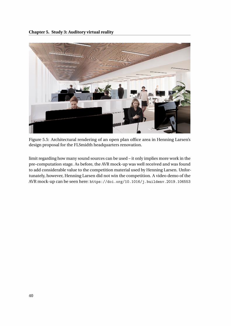
Chapter 5. Study 3: Auditory virtual reality
Figure 5.5: Architectural rendering of an open plan office area in Henning Larsen’sdesign proposal for the FLSmidth headquarters renovation.
limit regarding how many sound sources can be used – it only implies more work in thepre-computation stage. As before, the AVR mock-up was well received and was foundto add considerable value to the competition material used by Henning Larsen. Unfor-tunately, however, Henning Larsen did not win the competition. A video demo of theAVR mock-up can be seen here: https://doi.org/10.1016/j.buildenv.2019.106553
40

6 Study 4: Towards accurate real-time broadband virtual acoustics
The purpose of this study is to apply model order reduction techniques to furtheraccelerate the wave-based scheme of study 1 (paper P8). Moreover, another purpose isto extend the applicability of the scheme by developing an efficient high-frequencygeometrical acoustics solver, that could be coupled with the wave-based scheme(paper P7). These papers are summarized here below.
6.1 Paper P7
K. Gkanos, F. Pind, H. H. B. Sørensen, C.-H. Jeong. “Comparison of parallel implemen-tation strategies for the image source method for real-time virtual acoustics,” (2020).Currently under review in Applied Acoustics.
As shown in paper P5, the runtime r of the wave-based simulator grows roughly withr = af4
max, where a is a constant and fmax is the highest frequency of interest. This istypical of all wave-based simulation methods, but the constant a varies significantly,and thanks to the high-order accuracy and suitability for parallel computing, theconstant is low for the proposed numerical scheme of study 1. But this neverthelessmeans that extending the simulation range to very high frequencies is intractable. Atthe same time, in this very high frequency range, the room response is highly stochasticand the air attenuates a significant part of the sound energy, meaning that the highdeterministic precision of wave-based simulations is not as important in this range.Taken together, there is a very strong motivation for hybridizing different methods,where more approximate and faster methods are made to cover the high frequencyrange and more precise methods, like the one of study 1 and 2, cover the low-midfrequency range. This is particularly needed if the objective is to do simulations withinreal-time constraints.
For this purpose, we set out to develop an efficient geometrical acoustics simulator,to serve as the high frequency portion of the hybrid model. The simulator is a classic
41
Chapter 6. Study 4: Towards accurate real-time broadband virtual acoustics
image source / ray tracing hybrid solver. Various well known acceleration techniqueson the ray tracing part were implemented, and moreover, the ray tracing algorithmwas adapted to run on massively parallel HPC architectures. Ray tracing is inherentlyvery well suited for running in parallel, as each ray is independent of the other rays.However, the image source method is less suited for parallel computing, and thepurpose of paper P7 is to investigate how the method can effectively be implementedfor HPC architectures. Two different approaches are proposed and in the paper theyare compared.
The image source method is difficult to parallelize because of the inherent data de-pendency of the image source tree, where progeny image sources are dependent onthe parent image sources. Another important feature is that several image sources arecomputed which either represent invalid reflection paths or source positions that areinvisible to the receiver. This nature of the method motivated the two implementationstrategies.
The former strategy (method A) emphasizes reducing the computational work asmuch as possible, by computing each level of the image source tree sequentially andapplying validity and visibility checks during the computation of the sources. Thetrees are pruned whenever invalid sources arise, and the visibility check is only appliedon valid sources. This method is suitable for being run on multi-core CPUs, wherethe core count is low but the communication between cores is efficient. The lattermethod (method B), however, computes every image source completely independentlyof the other image sources. This implies that a much greater amount of computationalwork must be carried out, but the work can be parallelized with nearly 100% parallelefficiency, much like the ray tracing method. This makes the method better suitedfor running on massively parallel architectures such as GPUs, that have thousands ofcores.
The two implementations are compared in the paper. It is found that both approachesare able to compute image sources up to the third reflection order within real-timeconstraints for fairly complex rooms (≈ 200 surfaces). Moreover, in a comparisonstudy considering four different rooms, it is found that method A is faster for thegeometrically simpler rooms, but method B is faster for the more complex cases.Importantly, the runtime of method B is independent of the geometric layout of theroom, it only depends on the number of surfaces. In the paper, we discuss that moreroom types ought to be considered before more general conclusions can be drawn.Moreover, we suggest that it would be relevant to run method B not just on one GPU asis done in the paper, but on several GPUs, as the method will scale efficiently to severalGPUs due to the high parallel efficiency.
42

6.2. Paper P8
6.2 Paper P8
F. Pind, J. S. Hesthaven, B. M. Afkham, A. P. Engsig-Karup, C.-H. Jeong. “Stable time-domain model order reduction for fast wave-based room acoustic simulations,” (2020).Manuscript draft, to be submitted, likely to The Journal of the Acoustical Society ofAmerica.
Model order reduction is a fairly well established class of numerical techniques toreduce the size and complexity of numerical systems for solving parameterized dif-ferential equations, as discussed in Section 2.4. However, somewhat surprisingly, thetechniques have apparently not been applied to room acoustic simulations yet. In thispaper, we explore the potential of using these techniques, in particular the reducedbasis method, for efficiently simulating wave propagation in enclosures. We argue thatin virtual acoustics these methods can be highly applicable, e.g., in iterative design,where the acoustics of a space need to be evaluated for several different combinationsof geometries and surface materials, or in interactive virtual acoustics, where an effi-cient parametrized model can be used to solve the system for different source-receivercombinations at interactive rates.
A thorough description of the reduced basis method is given in the paper. The methodconsists of two stages, an offline stage and an online stage. In the offline stage, snap-shots of full model solutions are gathered for different parameter values and a problem-dependent reduced basis is constructed. A reduced model is obtained using a projec-tion of the reduced basis, and this reduced model can then be solved in the onlinestage at a much faster rate than the original model for new parameter values.
Standard reduction techniques are described, the proper orthogonal decomposition(POD), which typically uses a fine uniform discretization of the parameter space, andgreedy sampling, which is an iterative sampling process driven by an error estimator.Using greedy sampling techniques is known to reduce the cost of the offline stage.However, since error estimation is difficult in time dependent problems, we propose anovel data-driven greedy-POD sampling algorithm as a way to reduce the cost of theoffline stage. This algorithm is based on fitting a Gaussian regression model to theerror data and using the variance of the regression model as an error estimator.
The reduced basis method is applied on a number of 2D numerical problems, with bothfrequency independent and frequency dependent boundary conditions, using bothPOD reduction and the greedy-POD sampling algorithm. We show that problems canbe solved with good accuracy using much smaller numerical systems than the originalfull order models. We analyze the reducibility as a function of various simulationconditions, where we, among other things, find that the reduction potential increaseswith the problem size, which is beneficial for wave-based room acoustic simulations,which typically involve very large problem sizes.
43

Chapter 6. Study 4: Towards accurate real-time broadband virtual acoustics
The important topic of the numerical stability of the reduced order model is discussedtowards the end of the paper. A stability issue with the reduced models was discoveredin the later stages of the development work, when carrying out the above-mentionednumerical experiments. In general, the stability properties of full order models arenot inherited by the reduced order models. This causes problems when using thereduced models for long-time integration. This discovery forced us to approach theproblem in a different way. We utilize symplectic model reduction techniques, whichpreserve the structure of the full models in the reduced models, thereby preserving thestability properties. A 1D proof of concept test case with rigid boundaries using thesymplectic-based reduced model is given in the paper and indeed stability is preservedfor long-time integration.
It should be emphasized that this paper is still in the draft stage and it is our intentionto expand the work before submission takes place. A number of important issues thatcould be considered prior to submission are listed in the conclusion section of thepaper. The most pressing issue is to extend the stable reduced order model to handlefrequency dependent boundary conditions.
44

7 Conclusions
7.1 Concluding remarks and discussion
Room acoustic simulations have been studied for several decades now and powerfulsimulation tools exist on the market and in academia. Nevertheless, state-of-the-art simulators are still restricted by several well known shortcomings. Geometrical-acoustics-based simulators are unable to simulate various types of common roomssuch as open plan offices, classrooms and hospital wards with sufficient accuracy.Likewise, the auralizations and interactive virtual acoustics they produce are con-sidered inauthentic. Wave-based methods are known to be accurate, but have notreached widespread use in the industry due to excessive computation times. Fur-thermore, many common wave-based methods are ill-suited for handling complexgeometries, which has been shown to lead to large errors in complex-shaped rooms.The lack of accurate boundary modeling and boundary input data uncertainty is also aknown Achilles heel in room acoustic simulations. Finally, architects, stakeholders andother non-experts have a hard time relating to and working with sound and acoustics,because they lack digital tools that make acoustics more tangible and accessible.
In this PhD project, a wide range of topics relating to room acoustic simulations havebeen investigated. The intention of this work has been to contribute to the state of theart, by developing new methods that aim to address some of these above-mentionedissues. The hope is that, ultimately, this will lead to an improved building designprocess, resulting in better buildings with healthier indoor environments.
By harnessing the potential of state-of-the-art numerical methodology, in particularthe two closely related spectral element and discontinuous Galerkin methods, incombination with the power of modern massively parallel computer hardware, a newtype of wave-based simulation scheme has been developed. The scheme is shown tobe able to simulate large and complex-shaped rooms with high precision well into themid frequency range, within practical computation times. The high-order accuracy is
45

Chapter 7. Conclusions
shown to improve the cost-efficiency considerably, as compared to standard low-orderfinite element methods. Since room acoustic simulations involve simulating largespaces, over long simulation times and under stringent accuracy requirements, high-order methods are particularly well-suited for the task. Various important aspects suchas locally-reacting frequency dependent boundary conditions, curvilinear meshingand high-performance computing optimization are addressed and good performanceon all these aspects is demonstrated. This novel wave-based scheme is the contributionof study 1 (papers P1 and P5).
In study 2 (papers P3, P4 and P6), we consider the topic of accurate modeling of bound-ary conditions in time-domain wave-based simulations and uncertainty quantifica-tion of boundary input data. Two methods are proposed for modeling the extended-reaction behavior of room surfaces and both methods are shown to improve thesimulation accuracy considerably. The first method can be applied to any room sur-face type, but is only suited for modeling early reflections. The second method hasno such restrictions, but is confined to the class of porous absorbers. By combiningthese boundary modeling methods into the accelerated scheme of study 1, a powerfulscheme emerges that can accurately account for a wide range of room surface types.We show that using local-reaction or weighted angle-averaged approaches to modelboundary conditions can lead to large and perceptually noticeable errors. Additionally,in light of the known uncertainties in boundary input data, we propose a framework toquantify this uncertainty in room acoustic simulations. The framework can be used togauge the severity of the uncertainty and to identify where weak points in the inputdata and in the model are. The framework is applied on a small room test case and it isshown that the input data are too uncertain for the model to be able to predict roomacoustic parameters within just-noticeable thresholds.
An auditory virtual reality system is developed, subjectively validated and applied inpractice in study 3 (papers P2 and C1). The objective is to develop a system that can useaccurate room acoustic simulators, e.g., wave-based methods, as its backbone, suchthat the acoustics are rendered accurately enough in the AVR experience and for it tobe useful in building design. The system is thus based on an offline-online paradigm,where the offline pre-computation stage consists of the generation of accurate am-bisonics room impulse responses across a grid in the room and the online runtimestage is then driven by a virtual reality engine that produces the visuals, and a real-timeaudio engine that handles interpolation, spatial decoding and playback. Subjectivetests show that good localization is obtained when using the second order ambisonics,combined with the immersive visuals and allowing listener’s head movement. However,no correlation is found between the perceived realism or sound continuity and thegrid resolution. The grid resolution is, however, found to influence the perceived widthof the sound source. The system is applied to three real building design cases and waswell received by the design team and stakeholders.
46

7.2. Possible future work
Lastly, study 4 (papers P7 and P8) presents work on accelerating simulations further,using both numerical and computational techniques. First, model order reductiontechniques are applied on the wave-based simulator and it is shown that there appearsto be considerable potential for accelerating simulations using these techniques. Amethod for incorporating frequency dependent boundaries in the reduced model isproposed and shown to yield good agreements with the full model. A data-drivensampling strategy is also proposed to reduce the cost of the offline sampling stage. Astability issue in the reduced models is identified and a solution is proposed basedon symplectic model reduction techniques and demonstrated to work for the case ofrigid boundaries. Second, high-performance computing strategies are considered fora high-frequency geometrical acoustics simulator based on the image source method.Two approaches are proposed, one aimed at reducing the computational operationsas much as possible and the other aimed at reducing data dependency as muchas possible, making it more suited for parallel processing. It turns out to be casedependent which approach is more efficient: for simpler rooms the former approachis more efficient, but for more complex rooms the latter method is more efficient.
7.2 Possible future work
The topics considered in this thesis definitely merit further research. The task of simu-lating room acoustics with high accuracy, and preferably under real-time constraints, isextremely challenging. While good progress and interesting results have been achievedduring the course of the project, there are many avenues open for further research.These include:
• The results of paper P8 show that there appears to be a potential for using thereduced basis method to significantly reduce the computational cost in wave-based simulations. However, further analysis is required on more realistic casesthan the 1D and 2D cases considered in that paper, to assess how much thecost can actually be reduced in practice. This could include perceptual tests toevaluate how much fidelity can be sacrificed in the reduced model. Moreover,some important problems remain unsolved, particularly the incorporation offrequency dependent boundary conditions in the stable reduced model.
• Developing a SEM or DGFEM based room acoustic simulator solving the fre-quency domain governing equations is of interest. Simulating in the frequencydomain offers some advantages over time-domain simulations, e.g., the fre-quency sweep can be parallelized and often fewer frequency steps are neededthan time steps, due to the stringent stability criterion on time stepping. Ap-plying the reduced basis method in the frequency domain instead of the timedomain is also of interest, as this circumvents stability issues. However, otherchallenges arise in the frequency domain, e.g., carrying out an inverse transform
47

Chapter 7. Conclusions
that captures the transient details for auralization purposes is not straightforward[207].
• The proposed wave-based numerical scheme is particularly well suited for com-plex-shaped spaces. It could be of interest to apply spatial domain decomposi-tion, where the proposed scheme is coupled with more efficient methods whichare unable to handle the geometric details, such as the adaptive rectangulardecomposition method, where the bulk of the air domain away from the bound-aries is discretized by the ARD method. This might yield an even more efficientscheme. Previous spatial domain decomposition work can serve as inspirationhere [95, 96, 124].
• In cases where the geometry discretization results in a mesh with elements ofsignificantly different sizes, local time-stepping methods can be useful [223].Global time stepping implies that the time step is restricted according to thesmallest element on the mesh, which can be inefficient. Local time stepping canalleviate this by having high time resolutions in the smaller elements and coarsertime resolutions in the bigger elements. Extending the time stepping to arbitraryorder accuracy could also be relevant.
• All sound sources considered in this work distribute sound uniformly in alldirections. It is important to incorporate directive sound sources in the wave-based scheme to be able to model, e.g., a human speaker or loudspeakers in therooms. Inspiration can be had from previous work [69, 70, 224].
• Wave-geometrical hybrids have been mentioned in the thesis. Thanks to thework carried out in this project, we have now reached a stage where most of thebuilding blocks for such a system are ready. But what remains is to effectivelycombine the two approaches. Some questions in this respect remain unan-swered, e.g., how to calibrate simulation results such that they are compatibleand at what frequency the transition between methods should occur. Anotherinteresting hybridization strategy is to further divide between early and late re-flection modeling, e.g. when using wave-based simulators for interactive virtualacoustics.
• The coupling approach applied in paper P4 for modeling the extended-reactionbehavior of porous sound absorbers could be applied to different boundarytypes, e.g., vibrating airtight panels and perforated panels, which can exhibitstrong extended-reaction behavior. Furthermore, the method of paper P3 couldbe improved by using a more accurate three dimensional sound field splittingtechnique, yielding a more accurate estimate of the wave incidence angle. Thiscould be important for surfaces which have angle dependent properties that varysharply with the incidence angle.
48

7.2. Possible future work
• The validation and uncertainty quantification framework of paper P6 should beapplied to additional cases, to get a better understanding of boundary input dataweaknesses.
• As wave-based methods are becoming more tractable well into the mid andhigh frequency range, aspects such as surface scattering due to fine-grainedsurface roughness and air absorption start to become an issue. Previous workhas considered air absorption in time-domain wave-based simulations [81]. Inprinciple, the wave-based scheme proposed in this study can handle any type ofgeometry, including very fine geometrical details. But it remains to be seen whatinfluence this has on the computational performance, and whether approximatemethods to account for surface scattering can do a better job than modelinggeometrical details in the millimeter range.
49


Bibliography
[1] U.S. Environmental Protection Agency. Report to congress on indoor air quality:Volume 2. epa/400/1-89/001c. Technical report, 1989.
[2] C. Maschke, T. Rupp, K. Hecht, and C. Maschke. The influence of stressors onbiochemical reactions – a review of present scientific findings with noise. Int. J.Hyg. Environ. Health, 203(1):45–53, 2000.
[3] V. Blomkvist R. Ulrich C. A. Eriksen T. Theorell I. Hagerman, G. Rasmanis. Influ-ence of intensive coronary care acoustics on the quality of care and physiologicalstate of patients. Int. J. Cardiol., 98(2):267—270, 2005.
[4] K. P. Waye, E. Ryherd, B. Lindahl, and I. Bergbom. Relating the hospital soundenvironment to occupant psychological and physiological response. J. Acoust.Soc. Am., 123(5):3193–3193, 2008.
[5] T. Theorell R. Ulrich G. Rasmanis V. Blomkvist, C. A.Eriksen. Acoustics andpsychosocial environment in intensive coronary care. Occup. Environ. Med.,62(3):e1, 2005.
[6] A. Seddigh, E. Berntson, F. Jönsson, C. B. Danielson, and H. Westerlund. Theeffect of noise absorption variation in open-plan offices: A field study with across-over design. J. Environ. Psych., 44:34–44, 2015.
[7] G. W. Evans and D. Johnsson. Stress and open-office noise. J. Appl. Psych.,85(5):779–783, 2000.
[8] D. Abbot. Calming the office cacophony. Safety Health Pract., 22(1):34–36, 2004.
[9] N. A. Oseland and A. Burton. Quantifying the impact of environmental condi-tions on worker performance for inputting to a business case to justify enhancedworkplace design features. J. Build. Survey, Appr. Val., 1(2):151–164, 2012.
[10] B. M. Shield and J. E. Dockrell. The effects of noise on children at school: Areview. Build. Acoust., 10(2):97–116, 2003.
51
Bibliography
[11] M. Klatte, J. Hellbrück, J. Seidel, and P. Leistner. Effects of classroom acousticson performance and well-being in elementary school children: A field study.Environ. Behav., 42(5):659–692, 2010.
[12] ISO 3382-1. Acoustics – Measurement of room acoustic parameters – Part 1:Performance spaces. International organization for standardization, 2009.
[13] IEC 60268-16. Sound system equipment – Part 16: Objective rating of speechintelligibility by speech transmission index. International electrotechnical com-mission, 2011.
[14] M. Kleiner, B. I. Dalenbäck, and P. Svensson. Auralization – An overview. J. AudioEng. Soc, 41(11):861–875, 1993.
[15] M. Beig, B. Kapralos, K. Collins, and P. Mizra-Babei. An introduction to spatialsound rendering in virtual environments and games. Comput. Games J., 8:199–214, 2019.
[16] M. Aretz and M. Vorländer. Combined wave and ray based room acoustic simu-lations of audio systems in car passenger compartments, Part I: Boundary andsource data. Appl. Acoust., 76:82–99, 2014.
[17] V. Valimaki, J. D. Parker, L. Savioja, J. O. Smith, and J. S. Abel. Fifty years ofartificial reverberation. IEEE Trans. Audio, Speech, Lang. Proc., 20(5):1421–1448,2012.
[18] J. Xia, B. Xu, S. Pentony, J. Xu, and J. Swaminathan. Effects of reverberation andnoise on speech intelligibility in normal-hearing and aided hearing-impairedlisteners. J. Acoust. Soc. Am., 143(3):1523–1533, 2018.
[19] J. LoVetri, D. Mardare, and G. Soulodre. Modeling of the seat dip effect using thefinite-difference time-domain method. J. Acoust. Soc. Am., 100(4):2204–2212,1996.
[20] M. L. S. Vercammen. Sound concentration caused by curved surfaces. PhD thesis,Eindhoven University of Technology, The Netherlands, 2011.
[21] E. Nilsson. Decay processes in rooms with non-diffuse sound fields. Part II:Effect of irregularities. Build. Acoust., 11(2):133–143, 2004.
[22] Y. W. Lam. Issues for computer modelling of room acoustics in non-concert hallsettings. Acoust. Sci. Tech., 26(2):145–155, 2005.
[23] H. Kuttruff. Room Acoustics. Taylor & Francis, Abington, 5th edition, 2009.
[24] M. Vorländer. Computer simulations in room acoustics: Concepts and uncer-tainties. J. Acoust. Soc. Am., 133(3):1203–1213, 2013.
52

Bibliography
[25] C. H. Jeong, G. Marbjerg, and J. Brunskog. Uncertainty of input data for roomacoustic simulations. In Proc. Baltic-Nordic Acoust. Meet., 2016.
[26] F. Brinkmann, L. Aspöck, D. Ackermann, S. Lepa, M. Vorländer, and S. Weinzierl.A round robin on room acoustical simulation and auralization. J. Acoust. Soc.Am., 145(4):2746–2760, 2019.
[27] E. E. Videbæk. Implementation of acoustics in the design phase of a building.Master’s thesis, Technical University of Denmark, Denmark, 2015.
[28] M. S. Lauridsen. Embedded room acoustic modelling in parametric design.Master’s thesis, Technical University of Denmark, Denmark, 2017.
[29] M. R. Schroeder. Novel uses of digital computers in room acoustics. J. Acoust.Soc. Am., 33(11):1669, 1961.
[30] M. R. Schroeder and K. H. Kuttruff. On frequency response curves in rooms.Comparison of experimental, theoretical, and Monte Carlo results for the averagefrequency spacing between maxima. J. Acoust. Soc. Am., 34(1):76–80, 1962.
[31] A. Krokstad, S. Strom, and S. Soersdal. Calculating the acoustical room responseby the use of a ray tracing technique. J. Sound Vib., 8(1):118–125, 1968.
[32] G.M. Naylor. ODEON–Another hybrid room acoustical model. Appl. Acoust.,38(2–4):131–143, 1993.
[33] B.-I. Dalenbäck. A new model for room acoustic prediction and auralization. PhDthesis, Chalmers University of Technology, Sweden, 1995.
[34] W. Ahnert and R. Feistel. EARS auralization software. J. Audio Eng. Soc.,41(11):894–904, 1993.
[35] L. Simon J. Picaut and J.-D. Polack. A mathematical model of diffuse sound fieldbased on a diffusion equation. Acta Acust. Acust., 83(4):614–621, 1997.
[36] V. Valeau, J. Picaut, and M. Hodgson. On the use of a diffusion equation forroom-acoustic prediction. J. Acoust. Soc. Am., 119(3):1504–1513, 2006.
[37] J. M. Navarro, J. Escolano, and J. J. Lopez. Implementation and evaluation ofa diffusion equation model based on finite difference schemes for sound fieldprediction in rooms. Appl. Acoust., 73(6-7):659–665, 2012.
[38] J. B. Allen and D. A. Berkley. Image method for efficiently simulating small-roomacoustics. J. Acoust. Soc. Am., 65:943–950, 1979.
[39] B.-I. Dalenbäck. Room acoustic prediction based on a unified treatment ofdiffuse and specular reflection. J. Acoust. Soc. Am., 100(2):899–909, 1996.
53

Bibliography
[40] A. Wareing and M. Hodgson. Beam-tracing model for predicting sound fields inrooms with multilayer bounding surfaces. J. Acoust. Soc. Am., 118(4):2321–2331,2005.
[41] M. Kutruff. Simulierte nachhallkurven in rechteckräumen mit diffusem shallfeld(simulated reverberation curves in rectangular rooms with diffuse sound fields).Acustica, 25:333–342, 1971.
[42] G. I. Koutsouris, J. Brunskog, C.-H. Jeong, and F. Jacobsen. Combination of acous-tical radiosity and the image source method. J. Acoust. Soc. Am., 133(6):3963–3974, 2013.
[43] G. Marbjerg, J. Brunskog, C.-H. Jeong, and E. Nilsson. Development and vali-dation of a combined phased acoustical radiosity and image source model forpredicting sound fields in rooms. J. Acoust. Soc. Am., 138(3):1457–1468, 2015.
[44] J. S. Suh and P. A. Nelson. Measurement of transient response of rooms andcomparison with geometrical acoustic models. J. Acoust. Soc. Am., 105(4):2304–2317, 1999.
[45] C.-H. Jeong, J.-G. Ih, and J. H. Rindel. An approximate treatment of reflectioncoefficient in the phased beam tracing method for the simulation of enclosedsound fields at medium frequencies. Appl. Acoust., 69:601–613, 2008.
[46] Y. W. Lam. The dependence of diffusion parameters in a room acoustics predic-tion model on auditorium sizes and shapes. J. Acoust. Soc. Am., 100(4):2193–2203,1996.
[47] M. Hodgson. Evidence of diffuse surface reflections in rooms. J. Acoust. Soc. Am.,89(2):765–771, 1991.
[48] U. P. Svensson, R. I. Fred, and J. Vanderkooy. An analytic secondary source modelof edge diffraction impulse responses. J. Acoust. Soc. Am., 106(5):2331–2344,1999.
[49] R. R. Torres, U. P. Svensson, and M. Kleiner. Computation of edge diffraction formore accurate room acoustics auralization. J. Acoust. Soc. Am., 109(2):600–610,2001.
[50] X. Zeng, C. L. Christensen, and J. H. Rindel. Practical methods to define scatteringcoefficients in a room acoustics computer model. Appl. Acoust., 67:771–786,2006.
[51] L. Savioja and U. P. Svensson. Overview of geometrical room acoustic modelingtechniques. J. Acoust. Soc. Am., 138(2):708–730, 2015.
[52] D. Schröder. Physically based real-time auralization of interactive virtual envi-ronments. PhD thesis, RWTH Aachen, Germany, 2011.
54

Bibliography
[53] G. Marbjerg, J. Brunskog, and C.-H. Jeong. The difficulties of simulating theacoustics of an empty rectangular room with an absorbing ceiling. Appl. Acoust.,141:35–45, 2018.
[54] R. Courant, K.O. Friedrichs, and H. Lewy. Über die partiellen differenzengle-ichungen der mathematischen physik (About the partial difference equations ofmathematical physics). Math. Ann., 100:32–74, 1928.
[55] A. Hrennikoff. Solution of problems of elasticity by the framework method. J.Appl. Mech., 8(4):169–175, 1941.
[56] R. Courant. Variational methods for the solution of problems of equilibrium andvibrations. Bull. Am. Math. Soc., 49:1–23, 1943.
[57] Vidar Thomée. From finite differences to finite elements: A short history ofnumerical analysis of partial differential equations. J. Comput. Appl. Math.,128(1):1–54, 2001.
[58] T. Shuku. An analysis of the acoustic resonance of the body cavity. Toyota Eng.,21:1–7, 1969.
[59] T. Shuku and K. Ishihara. The analysis of the acoustic field in irregularly shapedrooms by the finite element method. J. Sound Vib., 29(1):67–76, 1973.
[60] A. Craggs. The use of simple three-dimensional acoustic finite elements fordetermining the natural modes and frequencies of complex shaped enclosures.J. Sound Vib., 23(3):331–339, 1972.
[61] A. Craggs. A finite element method for free vibration of air in ducts and roomswith absorbing walls. J. Sound Vib., 173(4):568–576, 1994.
[62] D. Botteldooren. Finite-difference time-domain simulation of low-frequencyroom acoustic problems. J. Acoust. Soc. Am., 98(6):3302–3308, 1995.
[63] O. Chiba, T. Kashiwa, H. Shimoda, S. Kagami, and I. Fukai. Finite-differencetime-domain simulation of low-frequency room acoustic problems. J. Acoust.Soc. Jap., 49:551–562, 1993.
[64] L. Savioja, T. J. Rinne, and T. Takala. Simulation of room acoustics with a 3-Dfinite difference mesh. In Proc. Int. Comput. Music Conf. (ICMC), Danish Instituteof Electroacoustic Music, pages 463–466, 1994.
[65] K. Kowalczyk and M. v. Walstijn. Modeling frequency-dependent boundaries asdigital impedance filters in FDTD and K-DWM room acoustics simulations. J.Audio Eng. Soc., 56(7/8):569–583, 2008.
[66] H. Jeong and Y. W. Lam. FDTD modelling of frequency dependent boundaryconditions for room acoustics. In Proc. 20th Int. Cong. Acoust. (ICA), 2010.
55

Bibliography
[67] M. Toyoda and S. Ishikawa. Frequency-dependent absorption and transmissionboundary for the finite-difference time-domain method. Appl. Acoust., 145:159–166, 2019.
[68] H. Jeong and Y. W. Lam. Source implementation to eliminate low-frequencyartifacts in finite difference time domain room acoustic simulation. J. Acoust.Soc. Am., 131(1):258–268, 2012.
[69] D. T. Murphy, A. Southern, and L. Savioja. Source excitation strategies for obtain-ing impulse responses in finite difference time domain room acoustics simula-tion. Appl. Acoust., 82:6–14, 2014.
[70] S. Bilbao, A. Politis, and B. Hamilton. Local time-domain spherical harmonicspatial encoding for wave-based acoustic simulation. IEEE Signal Proc. Letters,26(4):617–621, 2019.
[71] C. Spa, A. Rey, and E. Hernandez. A GPU implementation of an explicit compactFDTD algorithm with a digital impedance filter for room acoustics applications.IEEE/ACM Trans. Audio, Speech, Lang. Proc., 23(8):1368–1380, 2015.
[72] J. J. Lopez, D. Carnicero, N. Ferrando, and J. Escolano. Parallelization of thefinite-difference time-domain method for room acoustics modelling based onCUDA. Math. Comput. Mod., 57(7):1822–1831, 2013.
[73] S. Sakamoto. Phase-error analysis of high-order finite difference time domainscheme and its influence on calculation results of impulse response in closedsound field. Acoust. Sci. Tech., 28(5):295–309, 2007.
[74] J. van Mourik and D. Murphy. Explicit higher-order FDTD schemes for 3D roomacoustic simulation. IEEE/ACM Trans. Audio, Speech, Lang. Proc., 22(12):2003–2011, 2014.
[75] B. Hamilton and S. Bilbao. FDTD methods for 3-D room acoustics simulationwith high-order accuracy in space and time. IEEE/ACM Trans. Audio, Speech,Lang. Proc., 25(11):2112–2124, 2017.
[76] H.-O. Kreiss and J. Oliger. Comparison of accurate methods for the integrationof hyperbolic equations. Tellus, 24(3):199–215, 1972.
[77] C.-W. Shu. High-order finite difference and finite volume WENO schemesand discontinuous Galerkin methods for CFD. Int. J. Comp. Fluid Dynamics,17(2):107–118, 2003.
[78] J. S. Hesthaven and T. Warburton. Nodal Discontinuous Galerkin Methods –Algorithms, Analysis, and Applications. Springer, New York, 2008.
56

Bibliography
[79] S. Bilbao, B. Hamilton, J. Botts, and L. Savioja. Finite volume time domain roomacoustics simulation under general impedance boundary conditions. IEEE Trans.Audio, Speech, Lang. Proc., 24(1):161–173, 2016.
[80] S. Bilbao. Modeling of complex geometries and boundary conditions in finitedifference/finite volume time domain room acoustics simulation. IEEE Trans.Audio, Speech, Lang. Proc., 21(7):1524–1533, 2013.
[81] S. Bilbao and B. Hamilton. Wave-based room acoustics simulation: Explicit/im-plicit finite volume modeling of viscothermal losses and frequency-dependentboundaries. J. Audio Eng. Soc, 65(1/2):78–89, 2017.
[82] C.-W. Shu. Essentially non-oscillatory and weighted essentially non-oscillatoryschemes for hyperbolic conservation laws. In A. Quarteroni, editor, AdvancedNumerical Approximation of Nonlinear Hyperbolic Equations, pages 325–432.Springer, Berlin, 1998.
[83] S. Kirkup. The boundary element method in acoustics: A survey. Appl. Sci.,9(8):1642, 2019.
[84] I. Harari and T. J.R. Hughes. A cost comparison of boundary element and finiteelement methods for problems of time-harmonic acoustics. Comput. MethodsAppl. Mech. Eng., 97(1):77–102, 1992.
[85] N. Gumerov and R. Duraiswami. Fast Multipole Methods for the HelmholtzEquation in Three Dimensions. Elsevier Science, Amsterdam, 2005.
[86] T. Betcke, E. van’t Wout, and P. Gelat. Computationally efficient boundary ele-ment methods for high-frequency Helmholtz problems in unbounded domains.In Modern Solvers for Helmholtz Problems, pages 215–243. Birkhäuser, Basel,2017.
[87] J. A. Hargreaves, L. R. Rendell, and Y. W. Lam. A framework for auralization ofboundary element method simulations including source and receiver directivity.J. Acoust. Soc. Am., 145(4):2625–2637, 2019.
[88] M. R. Bai. Study of acoustic resonance in enclosures using eigenanalysis basedon boundary element methods. J. Acoust. Soc. Am., 91(5):2529–2538, 1992.
[89] J. A. Hargreaves. Time domain boundary element method for room acoustics.PhD thesis, University of Salford, United Kingdom, 2007.
[90] M. Ochmann. The source simulation technique for acoustic radiation problems.Acta Acust. Acust., 81(6):512–527, 1995.
[91] M. E. Johnson, S. J. Elliott, K-H. Baek, and J. Garcia-Bonito. An equivalentsource technique for calculating the sound field inside an enclosure containingscattering objects. J. Acoust. Soc. Am., 104(3):1221–1231, 1998.
57

Bibliography
[92] S. Lee. Review: The use of equivalent source method in computational acoustics.J. Comput. Acoust., 25(1):1630001, 2017.
[93] M. Hornikx, W. De Roeck, and W. Desmet. A multi-domain fourier pseudospectraltime-domain method for the linearized Euler equations. J. Comput. Physics,231(14):4759––4774, 2012.
[94] M. Hornikx, T. Krijnen, and L. van Harten. openPSTD: The open source pseu-dospectral time-domain method for acoustic propagation. Comput. Phys.Comm., 203:298–308, 2016.
[95] N. Raghuvanshi, R. Narain, and M. C. Lin. Efficient and accurate sound prop-agation using adaptive rectangular decomposition. IEEE Trans. Vis. Comput.Graphics, 15(5):789–801, 2009.
[96] R. Mehra, N. Raghuvanshi, L. Savioja, M. C. Lin, and D. Manocha. An efficientGPU-based time domain solver for the acoustic wave equation. Appl. Acoust.,73(2):83–94, 2012.
[97] M. Hornikx. Ten questions concerning computational urban acoustics. Build.Enviro., 106:409–421, 2016.
[98] B. Hamilton. Finite Difference and Finite Volume Methods for Wave-based Mod-elling of Room Acoustics. PhD thesis, The University of Edinburgh, Scotland,2016.
[99] V. Easwaran and A. Craggs. An application of acoustic finite element models tofinding the reverberation times of irregular rooms. Acta Acust. Acust., 82(1):54–64,1996.
[100] T. Okuzono, T. Otsuru, R. Tomiku, and N. Okamoto. Fundamental accuracy oftime domain finite element method for sound-field analysis of rooms. Appl.Acoust., 71(10):940–946, 2010.
[101] T. Okuzono, T. Otsuru, R. Tomiku, and N. Okamoto. Application of modifiedintegration rule to time-domain finite-element acoustic simulation of rooms. J.Acoust. Soc. Am., 132(2):804–813, 2012.
[102] T. Okuzono, T. Otsuru, R. Tomiku, and N. Okamoto. A finite-element methodusing dispersion reduced spline elements for room acoustics simulation. Appl.Acoust., 79:1–8, 2014.
[103] T. Okuzono, T. Yoshida, K. Sakagami, and T. Otsuru. An explicit time-domainfinite element method for room acoustics simulations: Comparison of the per-formance with implicit methods. Appl. Acoust., 104:76–84, 2016.
[104] COMSOL multiphysics modeling software. https://www.comsol.com/. Accessed:17.06.2020.
58

Bibliography
[105] A. T. Patera. A spectral element method for fluid dynamics: Laminar flow in achannel expansion. J. Comp. Phys., 54(3):468–488, 1984.
[106] I. Babuska and B.Q. Guo. The h, p and h-p version of the finite element method;basis theory and applications. Adv. Eng. Softw., 15(3):159–174, 1992.
[107] G.E. Karniadakis and S.J. Sherwin. Spectral/hp Element Methods for Computa-tional Fluid Dynamics. Oxford University Press, Oxford, 2nd edition, 2005.
[108] G. Seriani. A parallel spectral element method for acoustic wave modeling. J.Comp. Acoust., 5(1):53–69, 1997.
[109] S. Airiau, M. Azaiez, F.B. Belgacem, and R. Guivarch. Parallelization of spectralelement methods. In J. M. L. M. Palma, A. A. Sousa, J. Dongarra, and V. Hernandez,editors, High Performance Computing for Computational Science — VECPAR2002, pages 392–403. Springer, Berlin, 2003.
[110] W.H. Reed and T.R. Hill. Triangular mesh methods for the neutron transportequation. Technical report, Los Alamos Scientific Laboratory Report, LA-UR-73-479, 1973.
[111] R. Biswas, K. D. Devine, and J. E. Flaherty. Parallel, adaptive finite elementmethods for conservation laws. Appl. Num. Math., 14(1):255–283, 1994.
[112] T. Okuzono, N. Shimizu, and K. Sakagami. Predicting absorption characteristicsof single-leaf permeable membrane absorbers using finite element method in atime domain. Appl. Acoust., 151:172–182, 2019.
[113] T. Yoshida, T. Okuzono, and K. Sakagami. Time domain room acoustic solverwith fourth-order explicit FEM using modified time integration. Appl. Sci.,10(11):3750, 2020.
[114] H. Wang, I. Sihar, R. Pagan Munoz, and M. Hornikx. Room acoustics modellingin the time-domain with the nodal discontinuous Galerkin method. J. Acoust.Soc. Am., 145(4):2650–2663, 2019.
[115] H. Wang, J. Yang, and M. Hornikx. Frequency-dependent transmission boundarycondition in the acoustic time-domain nodal discontinuous Galerkin model.Appl. Acoust., 164:107280, 2020.
[116] H. Wang and M. Hornikx. Time-domain impedance boundary condition model-ing with the discontinuous Galerkin method for room acoustics simulations. J.Acoust. Soc. Am., 147(4):2534–2546, 2020.
[117] J. S. Bradley, H. Sato, and M. Picard. On the importance of early reflections forspeech in rooms. J. Acoust. Soc. Am., 113(6):3233–3244, 2003.
59

Bibliography
[118] W. M. Hartmann. Localization of sound in rooms. J. Acoust. Soc. Am., 74(5):1380–1391, 1983.
[119] E. Granier, M. Kleiner, B.-I. Dalenbäck, and P. Svensson. Experimental auraliza-tion of car audio installations. J. Audio Eng. Soc, 44(10):835–849, 1996.
[120] A. Southern, S. Siltanen, D. T. Murphy, and L. Savioja. Room impulse responsesynthesis and validation using a hybrid acoustic model. IEEE Trans. Audio,Speech, Lang. Proc., 21(9):1940–1952, 2013.
[121] M. Aretz. Combined wave and ray based room acoustic simulations of smallrooms. PhD thesis, RWTH Aachen, Germany, 2012.
[122] Z. H. Fu and J. W. Li. GPU-based image method for room impulse responsecalculation. Multim. Tools Applic., 75(9):5205–5221, 2016.
[123] M. Taylor, A. Chandak, Q. Mo, C. Lauterbach, C. Schissler, and D. Manocha.iSound: Interactive GPU-based Sound Auralization in Dynamic Scenes. Univer-sity of North Carolina at Chapel Hill, 2010.
[124] R. P. Munoz and M. Hornikx. Hybrid Fourier pseudospectral/discontinuousGalerkin time-domain method for wave propagation. J. Comp. Phys., 348:416–432, 2017.
[125] K. Attenborough. Acoustical characteristics of porous materials. Phys. Reports,82(3):179–227, 1982.
[126] M. Aretz and M. Vorländer. Efficient modelling of absorbing boundaries in roomacoustic FE simulations. Acta Acust. Acust., 96(6):1042–1050, 2010.
[127] E. A. G. Shaw. The acoustic wave guide. II. Some specific normal acousticimpedance measurements of typical porous surfaces with respect to normallyand obliquely incident waves. J. Acoust. Soc. Am., 25(2):231–235, 1953.
[128] C. Klein and A. Cops. Angle dependence of the impedance of a porous layer.Acustica, 44(4):258–264, 1980.
[129] D. B. Bliss. and S. E. Burke. Experimental investigation of the bulk reactionboundary condition. J. Acoust. Soc. Am., 71(3):546–551, 1982.
[130] D.J. Sides and K.A. Mulholland. The variation of normal layer impedance withangle of incidence. J. Sound Vib., 14(1):139–142, 1971.
[131] M. Hodgson and A. Wareing. Comparisons of predicted steady-state levels inrooms with extended- and local-reaction bounding surfaces. J. Sound Vib.,309(1):167–177, 2008.
60

Bibliography
[132] B. Yousefzadeh and M. Hodgson. Energy- and wave-based beam-tracing pre-diction of room-acoustical parameters using different boundary conditions. J.Acoust. Soc. Am., 132(3):1450–1461, 2012.
[133] T. Paris. On the coefficient of sound-absorption measured by the reverberationmethod,. Philos. Mag., 5:489–497, 1928.
[134] C.-H. Jeong. Guideline for adopting the local reaction assumption for porousabsorbers in terms of random incidence absorption coefficients. Acta Acust.Acust., 97(5):779–790, 2011.
[135] R. Tomiku, T. Otsuru, N. Okamoto, T. Okuzono, and T. Shibata. Finite elementsound field analysis in a reverberation room using ensemble averaged surfacenormal impedance. In Proc. 40th Int. Cong. Expo. Noise Cont. Eng., 2011.
[136] H. de Bree, R. Lanoye, S. de Cock, and J. van Heck. In situ, broad band methodto determine the normal and oblique reflection coefficient of acoustic materials.In Proc. Noise. Vib. Conf., 2005.
[137] J. Ducourneau, V. Planeau, J. Chatillon, and A. Nejade. Measurement of soundabsorption coefficients of flat surfaces in a workshop. Appl. Acoust., 70:710–721,2009.
[138] A. Richard, E. Fernandez-Grande, J. Brunskog, and C.-H. Jeong. Estimation ofsurface impedance at oblique incidence based on sparse array processing. J.Acoust. Soc. Am., 141(6):4115–4125, 2017.
[139] M. Nolan. Estimation of angle-dependent absorption coefficients from spatiallydistributed in situ measurements. J. Acoust. Soc. Am., 147(2):EL119–EL124, 2020.
[140] M. A. Biot. The theory of propagation of elastic waves in a fluid-saturated poroussolid. I. low frequency range. II. higher frequency range. J. Acoust. Soc. Am.,28:168–191, 1956.
[141] J. F. Allard and N. Atalla. Propagation of Sound in Porous Media: Modelling soundabsorbing materials. Wiley, West Sussex, 3rd edition, 2009.
[142] R. Panneton. Comments on the limp frame equivalent fluid model for porousmedia. J. Acoust. Soc. Am., 122(6):EL217–EL222, 2007.
[143] R. Panneton and N. Atalla. An efficient finite element scheme for solving thethree-dimensional poroelasticity problem in acoustics. J. Acoust. Soc. Am.,101(6):3287–3298, 1997.
[144] N. Atalla, R. Panneton, and P. Debergue. A mixed displacement-pressure formu-lation for poroelastic materials. J. Acoust. Soc. Am., 104(3):1444–1452, 1998.
61

Bibliography
[145] M. A. Hamdi N. Atalla and R. Panneton. Enhanced weak integral formulationfor the mixed (u,p) poroelastic equations. J. Acoust. Soc. Am., 109(6):3065–3068,2001.
[146] R. Lanoye, G. Vermeir, W. Lauriks, F. Sgard, and W. Desmet. Prediction of thesound field above a patchwork of absorbing materials. J. Acoust. Soc. Am.,123(2):793–802, 2008.
[147] J.-D. Chazot, E. Perrey-Debain, and B. Nennig. The partition of unity finiteelement method for the simulation of waves in air and poroelastic media. J.Acoust. Soc. Am., 135(2):724–733, 2014.
[148] Z. E. A. Fellah and C. Depollier. Transient acoustic wave propagation in rigidporous media: A time-domain approach. J. Acoust. Soc. Am., 107(2):683–688,2000.
[149] Z. E. A. Fellah, M. Fellah, W. Lauriks, and C. Depollier. Direct and inverse scatter-ing of transient acoustic waves by a slab of rigid porous material. J. Acoust. Soc.Am., 113(1):61–72, 2003.
[150] Z. E. A. Fellah, A. Wirgin, M. Fellah, N. Sebaa, C. Depollier, and W. Lauriks. Atime-domain model of transient acoustic wave propagation in double-layeredporous media. J. Acoust. Soc. Am., 118(2):661–670, 2005.
[151] D. K. Wilson. Relaxation-matched modeling of propagation through porousmedia, including fractal pore structure. J. Acoust. Soc. Am., 94(2):1136–1145,1993.
[152] D.K. Wilson. Simple, relaxational models for the acoustical properties of porousmedia. Appl. Acoust., 50(3):171–188, 1997.
[153] D. K. Wilson, V. E. Ostashev, and S. L. Collier. Time-domain equations for soundpropagation in rigid-frame porous media. J. Acoust. Soc. Am., 116(4):1889–1892,2004.
[154] O. Umnova and D. Turo. Time domain formulation of the equivalent fluid modelfor rigid porous media. J. Acoust. Soc. Am., 125(4):1860–1863, 2009.
[155] D. Dragna, P. Pineau, and P. Blanc-Benon. A generalized recursive convolutionmethod for time-domain propagation in porous media. J. Acoust. Soc. Am.,138(2):1030–1042, 2015.
[156] J. Zhao, M. Bao, X. Wang, H. Lee, and S. Sakamoto. An equivalent fluid modelbased finite-difference time-domain algorithm for sound propagation in porousmaterial with rigid frame. J. Acoust. Soc. Am., 143(1):130–138, 2018.
62

Bibliography
[157] J. Zhao, Z. Chen, M. Bao, H. Lee, and S. Sakamoto. Two-dimensional finite-difference time-domain analysis of sound propagation in rigid-frame porousmaterial based on equivalent fluid model. Appl. Acoust., 146:204–212, 2019.
[158] T. Okuzono and K. Sakagami. A frequency domain finite element solver foracoustic simulations of 3D rooms with microperforated panel absorbers. Appl.Acoust., 129:1–12, 2018.
[159] M. Toyoda and D. Eto. Prediction of microperforated panel absorbers using thefinite-difference time-domain method. Appl. Acoust., 86:110–124, 2019.
[160] N. Atalla and F. Sgard. Finite Element and Boundary Methods in StructuralAcoustics and Vibration. Taylor & Francis, Boca Raton, 2015.
[161] I. A. Drumm. Hybrid finite element/finite difference time domain techniquefor modelling the acoustics of surfaces within a medium. Acta Acust. Acust.,93:804–809, 2007.
[162] P. Dietrich. Modeling measurement uncertainty in room acoustics. Acta Polytech.,47(4-5):63–67, 2007.
[163] I. Witew and M. Vorländer. Uncertainties of room acoustical measurements—influence of the exact source and receiver position. In Proc. Inst. Acoust., 2011.
[164] W. L. Oberkampf and C. J. Roy. Verification and validation in scientific computing.Cambridge University Press, Cambridge, 2011.
[165] C. J. Roy and W. L. Oberkampf. A comprehensive framework for verification,validation and uncertainty quantification in scientific computing. Comput. Meth.Appl. Mech. Eng., 200:2132–2144, 2011.
[166] C. Cruz-Neira, D. J. Sandin, T. A. DeFanti, R. V. Kenyon, , and J. C. Hart. Thecave: Audio visual experience automatic virtual environment. Comm. ACM,35(6):64–72, 1992.
[167] B. Kapralos, M. R. Jenkin, and E. Milios. Virtual audio systems. Presence: Teleoper.Virtual Environ., 17(6):527–549, 2008.
[168] M. S. Gazzaniga, R. B. Ivry, and G. R. Mangun. Cognitive Neuroscience: TheBiology of the Mind. W. W. Norton, New York, 1998.
[169] P. Larsson, D. Vastfjall, and M. Kleiner. Better presence and performance invirtual environments by improved binaural sound rendering. In Aud. Eng. Soc.Conf.: 22nd Int. Conf.: Virtual, Synthetic, and Entertainment Audio, 2002.
[170] J. Broderick, J. Duggan, and S. Redfern. The importance of spatial audio inmodern games and virtual environments. In Proc. IEEE Games, Entert., Mediaconf. (GEM), 2018.
63

Bibliography
[171] D. Schröder, S. Pelzer, M. Vetterli, and M. Vorländer. Through the hourglass:A faithful audiovisual reconstruction of the old Montreux casino. Acoust. Aus.,43(1):49–57, 2015.
[172] D. Poirier-Quinot, B. N. J. Postma, and B. F. G. Katz. Virtual reconstructions ofthe Théâtre de l’Athénée for archeoacoustic study. In Proc. Int. Cong. Acoust.,2019.
[173] J. Y. Jeon and H. I. Jo. Three-dimensional virtual reality-based subjective evalua-tion of road traffic noise heard in urban high-rise residential buildings. Build.Environ., 148:468–477, 2019.
[174] G. M. Echevarria Sanchez, T. Van Renterghem, K. Sun, B. De Coensel, and D. Bot-teldooren. Using virtual reality for assessing the role of noise in the audio-visualdesign of an urban public space. Landsc. Urban Plan., 167:98–107, 2017.
[175] L. Picinali, A. Afonso, M. Denis, and B. F.G. Katz. Exploration of architecturalspaces by blind people using auditory virtual reality for the construction ofspatial knowledge. Int. J. Human-Computer Studies, 72(4):393–407, 2014.
[176] I. Muhammad, M. Vorländer, and S. J. Schlittmeier. Audio-video virtual realityenvironments in building acoustics: An exemplary study reproducing perfor-mance results and subjective ratings of a laboratory listening experiment. J.Acoust. Soc. Am., 146(3):EL310–EL316, 2019.
[177] H. Sato, H. Sato, M. Morimot, and Y. Nakai. Localization of intermittent soundwith head movement: Basic study on optimum temporal characteristics of acous-tic guide signals. Appl. Acoust., 101(1):58–63, 2016.
[178] M. Vorländer. Auralization: Fundamentals of Acoustics, Modelling, Simulation,Algorithms and Acoustic Virtual Reality. Springer, Berlin, 2008.
[179] J. Sandvad. Dynamic aspects of auditory virtual environments. In Audio Eng.Soc. Conv. 100, 1996.
[180] L. Savioja, J. Huopaniemi, T. Lokki, and R Vaananen. Creating interactive virtualacoustic environments. J. Audio Eng. Soc, 47(9):675–705, 1999.
[181] M. Vorländer, D. Schröder, S. Pelzer, and F. Wefers. Virtual reality for architecturalacoustics. J. Build. Perf. Sim., 8:15–25, 2015.
[182] S. Pelzer, L. Aspöck, D. Schröder, and M. Vorländer. Interactive real-time simula-tion and auralization for modifiable rooms. Acoust. Aus., 21(1):65–73, 2014.
[183] F. Wefers and M. Vorländer. Flexible data structures for dynamic virtual auditoryscenes. Virtual Reality, 22(4):281–295, 2018.
64

Bibliography
[184] C. Lauterbach, A. Chandak, and D. Manocha. Interactive sound rendering incomplex and dynamic scenes using frustum tracing. IEEE Trans. Vis. Comput.Graph., 13(6):1672–1679, 2007.
[185] A. Chandak, L. Antani, M. Taylor, and D. Manocha. Fast and accurate geometricsound propagation using visibility computations. Build. Acoust., 18(1-2):123–144,2011.
[186] Oculus spatializer. https://developer.oculus.com/downloads/package/oculus-spatializer-unity/. Accessed: 19.06.2020.
[187] Steam audio. https://valvesoftware.github.io/steam-audio/. Accessed:19.06.2020.
[188] Google resonance. https://resonance-audio.github.io/resonance-audio/. Ac-cessed: 19.06.2020.
[189] Audiokinetic Wwise. https://www.audiokinetic.com/products/wwise/. Ac-cessed: 19.06.2020.
[190] Fmod. https://www.fmod.com/. Accessed: 19.06.2020.
[191] M. A. Gerzon. Periphony: With-height sound reproduction. J. Audio Eng. Soc,21(1):2–10, 1973.
[192] S. Dance E. Ballestero, P. Robinson. Head-tracked auralisations for a dynamicaudio experience in virtual reality scenarios. In 24th Int. Cong. Sound Vib., 2017.
[193] A. Ahrens, M. Marschall, and T. Dau. Measuring and modeling speech intel-ligibility in real and loudspeaker-based virtual sound environments. HearingResearch, 377:307–317, 2019.
[194] Dalenbäck B.-I. and Strömberg M. Real time walkthrough auraliation – the firstyear. In Proc. Inst. Acoust., 2006.
[195] N. Raghuvanshi, J. Snyder, R. Mehra, M. Lin, and N. Govindaraju. Precomputedwave simulation for real-time sound propagation of dynamic sources in complexscenes. In ACM Trans. Graph. (proc. SIGGRAPH)., 2010.
[196] Project Acoustics. https://docs.microsoft.com/en-us/gaming/acoustics/what-is-acoustics. Accessed: 20.06.2020.
[197] R. Mehra, A. Rungta, A. Golas, M. Lin, and D. Manocha. WAVE: Interactivewave-based sound propagation for virtual environments. IEEE Trans. Vis. Comp.Graph., 21(4):434–442, 2015.
[198] L. Antani, A. Chandak, L. Savioja, and D. Manocha. Interactive sound propa-gation using compact acoustic transfer operators. ACM Trans. Graph., 31(1),2012.
65

Bibliography
[199] C. Schissler, R. Mehra, and D. Manocha. High-order diffraction and diffusereflections for interactive sound propagation in large environments. ACM Trans.Graph., 33(4), 2014.
[200] J. S. Hesthaven, G. Rozza, and B. Stamm. Certified Reduced Basis Methods forParametrized Partial Differential Equations. Springer International Publishing,2016.
[201] D. Amsallem, J. Cortial, and C. Farhat. Towards real-time computational-fluid-dynamics-based aeroelastic computations using a database of reduced-orderinformation. AIAA J., 48(9):2029–2037, 2010.
[202] Stable Galerkin reduced order models for linearized compressible flow. J. Com-put. Physics, 228(6):1932–1946, 2009.
[203] S. Giere. Numerical and Analytical Aspects of POD-Based Reduced-Order Mod-eling in Computational Fluid Dynamics. PhD thesis, Free University of Berlin,Germany, 2016.
[204] Y. Chen, J. S. Hesthaven, Y. Maday, and J. Rodríguez. Certified reduced basismethods and output bounds for the harmonic Maxwell’s equations. SIAM J. Sci.Comput., 32(2):970–996, 2010.
[205] M. Ganesh, J.S. Hesthaven, and B. Stamm. A reduced basis method for elec-tromagnetic scattering by multiple particles in three dimensions. J. Comput.Physics, 231(23):7756–7779, 2012.
[206] M.A. Grepl. Reduced-basis approximation and a posteriori error estimation forparabolic partial differential equations. PhD thesis, Massachusetts Institute ofTechnology, United States, 2005.
[207] C. Bigoni and J. S. Hesthaven. Simulation-based anomaly detection and damagelocalization: An application to structural health monitoring. Comput. Meth.Appl. Mech. Eng., 363:112896, 2020.
[208] U. Hetmaniuk, R. Tezaur, and C. Farhat. Review and assessment of interpolatorymodel order reduction methods for frequency response structural dynamics andacoustics problems. Int. J. Num. Meth. Eng., 90(13):1636–1662, 2012.
[209] J. Herrmann, M. Maess, and L. Gaul. Substructuring including interface reduc-tion for the efficient vibro-acoustic simulation of fluid-filled piping systems.Mech. Sys. Sig. Proc., 24(1):153–163, 2010.
[210] R. Srinivasan Puri, D. Morrey, A. J. Bell, J. F. Durodola, E. B. Rudnyi, and J. G.Korvink. Reduced order fully coupled structural–acoustic analysis via implicitmoment matching. Appl. Math. Mod., 33(11):4097–4119, 2009.
66

Bibliography
[211] E. Lappano, M. Polanz, W. Desmet, and D. Mundo. A parametric model orderreduction technique for poroelastic finite element models. J. Acoust. Soc. Am.,142(4):2376–2385, 2017.
[212] E. Creixell-Mediante, J. S. Jensen, F. Naets, J. Brunskog, and M. Larsen. Adaptiveparametric model order reduction technique for optimization of vibro-acousticmodels: Application to hearing aid design. J. Sound Vib., 424:208–223, 2018.
[213] A. van de Walle, F. Naets, E. Deckers, and W. Desmet. Stability-preserving modelorder reduction for time-domain simulation of vibro-acoustic FE models. Int. J.Num. Meth. Eng., 109(6):889–912, 2017.
[214] S. van Ophem, O. Atak, E. Deckers, and W. Desmet. Stable model order reductionfor time-domain exterior vibro-acoustic finite element simulations. Comput.Meth. Appl. Mech. Eng., 325:240–264, 2017.
[215] V. Pereyra and B. Kaelin. Fast wave propagation by model order reduction. Elec.Trans. Num. Anal., 30:406–419, 2008.
[216] B. M. Afkham and J. S. Hesthaven. Structure preserving model reduction ofparametric Hamiltonian systems. SIAM J. Sci. Comput., 39(6):A2616–A2644,2017.
[217] P.-O. Persson and G. Strang. A simple mesh generator in Matlab. SIAM Review,46(2):329–345, 2004.
[218] A. Karakus, N. Chalmers, K. Swirydowicz, and T. Warburton. A GPU accelerateddiscontinuous Galerkin incompressible flow solver. J. Comput. Phys., 390:380–404, 2019.
[219] K. Swirydowicz, N. Chalmers, A. Karakus, and T. Warburton. Acceleration oftensor-product operations for high-order finite element methods. Int. J. HighPerf. Comput. Appl., 33(4):735–757, 2019.
[220] D. S. Medina, A. St-Cyr, and T. Warburton. OCCA: A unified approach to multi-threading languages, 2014. Article preprint.
[221] C. Geuzaine and J.-F. Remacle. Gmsh: a three-dimensional finite element meshgenerator with built-in pre- and post-processing facilities. Int. J. Num. MethodsEng., 79(11):1309–1331, 2009.
[222] M. J. Grote, M. K., F. Nataf, and F. Assous. Time-dependent wave splitting andsource separation. J. Comput. Phys., 330:981–996, 2017.
[223] M. Dumbser, M. Kaser, and E. F. Toro. An arbitrary high-order DiscontinuousGalerkin method for elastic waves on unstructured meshes – V. Local time step-ping and p-adaptivity. Geophys. J. Int., 171(2):695–717, 2007.
67

Bibliography
[224] F. Georgiou and M. Hornikx. Incorporating directivity in the Fourier pseu-dospectral time-domain method using spherical harmonics. J. Acoust. Soc.Am., 140(2):855–865, 2016.
68

PAPER P1
69

Time domain room acoustic simulations using the spectralelement methoda)
Finnur Pind,1,b) Allan P. Engsig-Karup,2 Cheol-Ho Jeong,3 Jan S. Hesthaven,4
Mikael S. Mejling,2 and Jakob Strømann-Andersen11Henning Larsen, Copenhagen, Denmark2Scientific Computing Group, Department of Applied Mathematics and Computer Science,Technical University of Denmark, Kongens Lyngby, Denmark3Acoustic Technology Group, Department of Electrical Engineering, Technical University of Denmark,Kongens Lyngby, Denmark4Chair of Computational Mathematics and Simulation Science, Ecole Polytechnique Federale de Lausanne,Lausanne, Switzerland
(Received 4 April 2019; revised 7 May 2019; accepted 8 May 2019; published online 5 June 2019)
This paper presents a wave-based numerical scheme based on a spectral element method, coupled
with an implicit-explicit Runge-Kutta time stepping method, for simulating room acoustics in the
time domain. The scheme has certain features which make it highly attractive for room acoustic simu-
lations, namely (a) its low dispersion and dissipation properties due to a high-order spatio-temporal
discretization; (b) a high degree of geometric flexibility, where adaptive, unstructured meshes with
curvilinear mesh elements are supported; and (c) its suitability for parallel implementation on modern
many-core computer hardware. A method for modelling locally reacting, frequency dependent imped-
ance boundary conditions within the scheme is developed, in which the boundary impedance is
mapped to a multipole rational function and formulated in differential form. Various numerical
experiments are presented, which reveal the accuracy and cost-efficiency of the proposed numerical
scheme.VC 2019 Acoustical Society of America. https://doi.org/10.1121/1.5109396
[LS] Pages: 3299–3310
I. INTRODUCTION
Room acoustic simulations are used in many fields, for
example, in building design,1 virtual reality,2 entertainment,3
automotive design,4 music,5 and hearing research.6 Since
their inception in the 1960s,7,8 room acoustic simulations
have primarily been carried out by means of geometricalacoustics methods,9 such as the ray tracing method,10 the
image source method,11 or the beam tracing method.12 In
these methods, several simplifying approximations regarding
sound propagation and reflection are made, which make the
computational task more manageable. These approximations
will, however, deteriorate the accuracy of the simulation
because various important wave phenomena, such as diffrac-
tion, interference, and scattering, are not accurately captured.
Wave phenomena will be prominent in rooms where the
room dimensions and sizes of obstacles are comparable to
the wavelength of the acoustic wave. Small to medium sized
rooms, and low to mid frequencies, are, here, of primary
concern.13 However, large rooms can also exhibit wave phe-
nomena, e.g., the seat-dip effect.14 Another problem associ-
ated with geometrical acoustics methods is that they require
simplified three-dimensional (3D) models, made up of
coarse planar polygons. Fine geometrical details are
typically replaced by assigning scattering coefficients to pla-
nar surfaces, and these coefficients are often based on crude
visual inspection.15 Instead of using simplified 3D models, it
would be more accurate to model directly the complex and
detailed geometry typically found in architectural models.16
Thanks to the continuous advances in computation power
and scientific computing theory, the wave-based methods are
becoming a viable alternative for room acoustic simulations. In
these methods the governing physics equations are solved
numerically, and they are therefore, from a physical point of
view, more accurate than their geometrical counterparts, since
all wave phenomena is inherently accounted for.17 Wave-based
methods that have been applied to room acoustic simulations
include the finite-difference time-domain (FDTD) method,18 the
boundary element method (BEM),19 the linear finite element
method (h-FEM),20 the equivalent source method (ESM),21 the
finite volume method (FVM),22 and the pseudospectral time-
domain (PSTD) method.23 A major drawback of the wave-based
methods is the large computational effort needed.24 Various
studies have been carried out to bring down computation times,
e.g., parallel implementations of algorithms utilizing many-core
hardware, such as GPU’s,25 hybridization of different algorithm
types,4,26,27 and, recently, the usage of high-order numerical
methods, which have the potential of being cost-efficient,28 has
been investigated within the context of room acoustics.29,30
The primary purpose of this paper is to present a numer-
ical scheme based on a spectral element method (SEM)31–33
adapted for time domain room acoustic simulations, and to
assess the suitability of using the SEM for this task. The
SEM is known to be well-suited for cost-effective
a)Portions of this work were presented in “Room acoustic simulations using
high order spectral element methods,” Proceedings of Euronoise 2018,
Heraklion, Crete, May 2018.b)Also at: Acoustic Technology Group, Department of Electrical Engineering,
Technical University of Denmark, Kongens Lyngby, Denmark. Electronic
mail: [email protected]
J. Acoust. Soc. Am. 145 (6), June 2019 VC 2019 Acoustical Society of America 32990001-4966/2019/145(6)/3299/12/$30.00

simulations of large scale problems over long simulation
times due to a high-order polynomial basis discretization,
which leads to small numerical dispersion and dissipation
errors.34 Furthermore, the SEM is capable of operating on
unstructured, adaptive meshes with curvilinear mesh ele-
ments, making it highly suitable for simulating complex
geometries. Finally, the SEM has also been shown to be
well-suited for parallel computing.35,36 In the scheme pre-
sented here, time stepping is done by means of an implicit-
explicit high-order Runge-Kutta solver,37 ensuring computa-
tional efficiency, robustness, and the maintenance of global
high-order accuracy. A method for incorporating locally
reacting, frequency dependent impedance boundary condi-
tions in the scheme is presented.
The SEM has several advantages compared to the other
wave-based methods found in the literature. The FDTD
method and the PSTD method are ill-suited for dealing with
complex geometries.38,39 The FVM overcomes this drawback
of limited geometrical flexibility,22 however, another chal-
lenge with the FVM is a flux reconstruction procedure that,
despite recent progress, is not straightforward to extend to
arbitrarily high-order accuracy in two and three spatial
dimensions.40,41 The BEM has the benefit of needing only to
discretize the boundary surface instead of the domain volume;
however, in the BEM operators are dense. Typically the
FEM, which has sparse operators and where the domain vol-
ume is discretized, is considered faster than the BEM unless
the volume to surface area becomes very large.24 In addition,
there are other challenges relating to uniqueness of solutions
in the BEM.42 High-order FEM, typically referred to as the
hp-FEM, is another option.43 The hp-FEM and the SEM are
based on the same underlying theoretical framework and pos-
sess similar properties, while differing in implementation.
The key distinction between the hp-FEM and the SEM is
whether the expansion is modal or nodal. In the hp-FEM the
expansion basis is normally modal, i.e., the basis functions
are of increasing order (hierarchical). In a modal expansion
the expansion coefficients do not have any particular physical
meaning. In contrast, in the SEM the expansion basis is a
non-hierarchical Lagrange basis, which consists of polyno-
mials of arbitrary order, with support on the element.
Importantly, the nodal expansion coefficients are associated
with the solution values at the nodal points, hence, these can
be interpreted readily. The discontinuous Galerkin finite ele-
ment method (DGFEM) is another method which stems from
a similar theoretical framework as the SEM. Its main draw-
backs relative to the SEM are that it requires more degrees of
freedom (DOF), and a flux reconstruction between elements
must be computed. However, it relies only on local weak for-
mulations defined for elements rather than for the full domain
as in the SEM, which makes it possible to exploit the result-
ing locality in parallelization. The hp-FEM, SEM, and
DGFEM have similar geometric flexibility.44
The paper is structured as follows. In Sec. II, the govern-
ing acoustics equations and the boundary condition formula-
tion are presented. In Sec. III, the proposed numerical scheme
is described. Certain numerical properties of the scheme, such
as numerical dispersion and dissipation, and its computational
efficiency, are analyzed in Sec. IV. Section V presents various
simulation results made using the proposed scheme, and finally
some concluding remarks are given in Sec. VI.
II. GOVERNING EQUATIONS AND BOUNDARYCONDITIONS
Acoustic wave propagation in a lossless medium in a d-dimensional enclosure is governed by the following system of
two coupled linear first-order partial differential equations,
vt ¼ 1
qrp;
pt ¼ qc2r v;inX 0; t½ ; (1)
where p(x,t) is the sound pressure, v(x,t) is the particle
velocity, x is the position in space of the domain X, t is time,
q is the density of the medium, and c is the speed of sound in
air (q¼ 1.2 kg/m3 and c¼ 343m/s in this study). These
equations correspond to the linearized Euler and continuity
equation without flow. This system is exactly equivalent to
the more commonly used second-order wave equation.
Sufficient boundary conditions must be supplied with
the system in Eq. (1), and in room acoustics it is natural to
define the boundary conditions in terms of the complex, fre-
quency dependent surface impedance Z(x), which can be
estimated from material models or measurements.45,46 The
pressure and the particle velocity at the boundary are related
through the surface impedance in the frequency domain via
vn xð Þ ¼ p xð ÞZ xð Þ ¼ p xð ÞY xð Þ; (2)
where x is the angular frequency, p and vn ¼ v n are the
Fourier transforms of the pressure and particle velocity at the
boundary, respectively, n is the surface normal unit vector, and
Y(x) is the boundary admittance, which is convenient to use
when implementing frequency dependent boundary conditions
into the linearized Euler equations. The boundary admittance
can be approximated as a rational function on the form
Y xð Þ ¼ a0 þ þ aN jxð ÞN
1þ þ bN jxð ÞN; (3)
which can be rewritten by using partial fraction decomposi-
tion as47
Y xð Þ ¼ Y1 þXQk¼1
Ak
kk jx
þXSk¼1
Bk þ jCk
ak þ jbk jxþ Bk jCk
ak jbk jx
; (4)
where Q is the number of real poles kk and S is the number
of complex conjugate pole pairs ak6 jbk used in the rational
function approximation. Y1, Ak, Bk, and Ck are numerical
coefficients. Any number of poles can be chosen, one strat-
egy being to choose enough poles such that the error in the
multipole approximation of the boundary admittance is
below a predefined threshold.
3300 J. Acoust. Soc. Am. 145 (6), June 2019 Pind et al.

Equation (2) can be transformed to the time domain by
means of an inverse Fourier transform,
vnðtÞ ¼ðt1
pðt0Þyðt t0Þ dt0: (5)
Then, by applying an inverse Fourier transform on Eq. (4)
and inserting it into Eq. (5), the expression for the velocity at
the boundary becomes
vnðtÞ ¼ Y1pðtÞ þXQk¼1
Ak/kðtÞ
þXSk¼1
2 Bkwð1Þk ðtÞ þ Ckw
ð2Þk ðtÞ
h i; (6)
where /k; wð1Þk , and wð2Þ
k are so-called accumulators. They
are determined by the following set of ordinary differential
equations (ODEs):
d/k
dtþ kk/k tð Þ ¼ p tð Þ;
dw 1ð Þk
dtþ akw
1ð Þk tð Þ þ bkw
2ð Þk tð Þ ¼ p tð Þ;
dw 2ð Þk
dtþ akw
2ð Þk tð Þ bkw
1ð Þk tð Þ ¼ 0: (7)
This approach is often called the auxiliary differential equa-
tions (ADE) method in the literature,47–49 and has the benefit
of being computationally efficient because solving a small
set of ODEs requires only relatively minor computations.
Furthermore, this approach has low memory requirements
because only one time step history of accumulator values
must be stored.
III. NUMERICAL DISCRETIZATION
In this section, a high-order numerical scheme for the
solution of Eq. (1) in two and three spatial dimensions is
derived. High-order methods are methods which have a global
error convergence rate OðhPÞ of at least third order (P> 2),
where h is the mesh element side length. In this study, trian-
gular mesh elements are used in two dimensional (2D) simu-
lations, and hexahedral elements are used in 3D simulations,
although elements of different shapes can be used.
A. Spatial discretization
The domain X is partitioned into a set of non-
overlapping elements Xn, n¼ 1,…,Nel. A set of nodes is cho-
sen and mapped into each element, making up a total of Knodes across the mesh and having coordinates xi, i¼ 1,…,K.A finite element approximation space V of globally continu-
ous, piecewise polynomial functions of degree at most P is
introduced, V ¼ f/ 2 C0ðXÞ; 8n 2 f1;…; Nelg;/ðnÞ 2 PPg.As such, the global basis functions / are defined by patching
together local polynomial nodal basis functions /(n), which
are defined locally on each element and in this study taken to
be Lagrange polynomials of order P. To support order P basis
functions, each element must contain KP¼ (Pþ 1) (Pþ 2)/2
nodes in two dimensions for the triangular elements and
KP¼ (Pþ 1)3 nodes in three dimensions for the hexahedral
elements.44 Figure 1 shows an example of a 2D mesh of a
rectangular domain, supporting P¼ 4 order basis functions.
The weak formulation of the governing equations,
through the use of the divergence theorem on the pressure
equation in Eq. (1), takes the following form:
ðXvt/ dX ¼ 1
q
ðXrp/ dX;
ðXpt/ dX ¼ qc2
ðC/n v dC
ðXv r/ dX
;
(8)
where C denotes the boundary of X. Now, introduce a truncatedseries expansion for the unknown variables v and p in Eq. (8)
vðx; tÞ XKi¼1
viðtÞNiðxÞ;
pðx; tÞ XKi¼1
piðtÞNiðxÞ; (9)
where Ni(x) 2 V is the set of global finite element basis
functions, possessing the cardinal property Ni(xj)¼ dij.Substituting the approximations in Eq. (9) for v and p into Eq.(8) and choosing / 2 fNiðxÞgKi¼1 to define a nodal Galerkin
scheme results in the following semi-discrete system:
Mv0x ¼ 1
qSxp; Mv0y ¼ 1
qSyp; Mv0z ¼ 1
qSzp;
Mp0 ¼ qc2 STx vx þ STy vy þ STz vz vnB
; (10)
where vx, vy, vz represent the x,y,z components of the particle
velocity, vn is computed using Eq. (6) and where the follow-
ing global matrices have been introduced:
Mij ¼ðXNj Ni dX; Sx;ðijÞ ¼
ðXðNjÞx Ni dX;
Sy;ðijÞ ¼ðXðNjÞy Ni dX; Sz;ðijÞ ¼
ðXðNjÞz Ni dX;
Bij ¼ðCNj Ni dC; (11)
FIG. 1. An example of a mesh of a 2D rectangular domain using triangular
elements and having nodes for supporting P¼ 4 basis functions. The mesh
is made up of Nel¼ 24 elements and contains 221 DOF (nodes).
J. Acoust. Soc. Am. 145 (6), June 2019 Pind et al. 3301

where the x,y,z subscripts in the integrals denote differentia-
tion. In Eq. (10)M is typically called the mass matrix and S iscalled the stiffness matrix. To determine these matrices, it is
convenient to introduce the concept of a local element matrix.Due to the nature of the global piecewise basis functions,
the integrals in Eq. (11) are only non-zero when the nodes i,jbelong to the same element.32 This means that two basis func-
tions Ni and Nj only contribute toward entries Mij when xi, xj2 Xn, due to the local support of the basis functions. This
leads to the definition of the local element matrices as
MðnÞij ¼
ðXn
NðnÞi N
ðnÞj dXn;
SðnÞx;ðijÞ ¼
ðXn
NðnÞi ðNðnÞ
j Þx dXn;
SðnÞy;ðijÞ ¼
ðXn
NðnÞi ðNðnÞ
j Þy dXn;
SðnÞz;ðijÞ ¼
ðXn
NðnÞi ðNðnÞ
j Þz dXn;
i; j ¼ 1…KP: (12)
From the local element matrices, it is possible to assemble
the global matrices in Eq. (11) by iterating over the elements
and summing the element contributions, relying on the prop-
erty of domain decomposition, e.g.,
Mij ¼ðXNiNj dX ¼
XNel
n¼1
ðXn
NðnÞi N
ðnÞj dXn; (13)
where the integrals may be zero. The element matrices are
therefore dense, whereas the global matrices are sparse.
B. Spatial integration and nodal/modal duality
To compute the element matrices in Eq. (12), it is con-
venient to introduce a special element called the reference
element Xr. In two dimensions it is a triangle, given by
I 2 ¼ fr ¼ ðr; sÞjðr; sÞ 1; r þ s 0g; (14)
and in three dimensions it is a hexahedron, given by
I 3 ¼ fr ¼ ðr; s; tÞj 1 ðr; s; tÞ 1g: (15)
On these elements one can define a hierarchical modal basis,
as opposed to the nodal basis discussed above. This implies a
possible modal/nodal duality in the representation of the local
solutions that can be exploited for exact integration, relying
on the orthogonal properties of the local modal basis functions
without resorting to numerical quadrature rules. When using a
modal basis, an unknown function is represented as
uðrÞ ¼XPj¼0
~ujwjðrÞ; r 2 I d; (16)
where wj are the modal basis functions and the coeffi-
cients ~uj are weights. On I 2 a basis proposed by
Dubiner50 is chosen, where the reference triangle ele-
ment is first mapped to a unit square quadrilateral ele-
ment by the mapping
T : r; sð Þ ! a; bð Þ; T r; sð Þ ¼ 21þ r
1 s 1 ; s
; (17)
where (a,b) are the coordinates in the quadrilateral element.
This allows for defining a modal basis in terms of tensor
products from the one-dimensional (1D) reference element
I 1 ¼ ½1; 1. The intra-element nodal distribution of the col-
location points r of the 1D reference element used in this
study is of the Legrende-Gauss-Lobatto (LGL) kind. Using
this nodal distribution avoids Runge’s phenomenon.44 Now,
the 2D modal basis is defined as
wpqðr; sÞ ¼ /apðrÞ/b
qðsÞ; (18)
where
/ap rð Þ ¼ P0;0
p rð Þ; /bq sð Þ ¼ 1 s
2
2
P2pþ1;0q sð Þ; (19)
and where Pa;bp ðzÞ is the pth-order Jacobi polynomial with
parameters a, b. By constructing the basis functions wpq in
this manner, they become orthonormal on I 2.
On I 3, a similar orthonormal modal basis is constructed
using a tensor product of Jacobi polynomials
wðr; s; tÞ ¼ P0;0i ðrÞ P0;0
j ðsÞ P0;0k ðtÞ; i; j; k ¼ 0;…;P:
(20)
The function values of the nodes u used in the nodal
representation and the weights ~u used in the modal represen-
tation of u relate to each other through
Vu ¼ ~u; (21)
where V is the generalized Vandermonde matrix with
V ij ¼ wjðriÞ; i; j ¼ 1;…;Pþ 1: (22)
Utilizing this, the ith local nodal basis function on the refer-
ence element can be expressed as44
NiðrÞ ¼XPþ1
n¼1
ðVTÞ1i;n wnðrÞ: (23)
Inserting Eq. (23) into the expression defining the element
mass matrixM on the reference element yields
Mij ¼XPþ1
n¼1
ðVTÞ1i;n ðVTÞ1
j;n ¼ ðVVTÞ1; (24)
using the orthonormality of the chosen modal basis and thus
avoiding the use of numerical quadrature rules. The connec-
tion to the mass matrix in Eq. (12) is defined by the coordi-
nate mapping between the reference element and any
element in the physical space
3302 J. Acoust. Soc. Am. 145 (6), June 2019 Pind et al.

MðnÞij ¼
ðXn
wiðxÞwjðxÞ dXn ¼ðXr
JðnÞwiðrÞwjðrÞ dXr;
(25)
where J ðnÞ is the Jacobian of the coordinate mapping
n : xðnÞ ! r.
Next, write the derivative of the ith local basis function
as
@
@rNi r; s; tð Þ ¼
XPþ1
n¼1
@
@rNi rn; sn; tnð ÞNn r; s; tð Þ: (26)
Inserting the above into the expression defining the element
stiffness matrix in Eq. (12) one finds that44
Sr ¼ MDr; (27)
where
Dr ¼ VrV1; (28)
is a differentiation matrix and
Vr; ijð Þ ¼@
@rwj ri; sið Þ: (29)
The remaining element matrices Ss and St are defined simi-
larly, and again the Jacobian coordinate mapping is used to
map between the reference element and an arbitrary element
in the mesh.
C. Time stepping and stability
In order to solve the ODE system in Eq. (10) efficiently,
an explicit time stepping method is preferred.51 Explicit time
stepping comes with conditional stability, which sets an upper
bound on the time step size Dt. In the proposed numerical
scheme there are two mechanisms at play which influence the
maximum allowable time step: (1) the usual global Courant-
Friedrichs-Lewy (CFL) condition, where Dt C1=maxjkij,where ki represents the eigenvalues of the spatial discretiza-
tion,34 and C1 is a constant depending on the size of the stabil-
ity region of the time stepping method; (2) the stiffness of the
ADE equations [Eq. (7)]. For certain boundary conditions, the
ADE equations can become stiff, which puts an excessively
strict restriction on the time step. This motivates the usage of
an implicit-explicit time stepping method, where the main
SEM semi-discrete system [Eq. (10)] is integrated explicitly
in time, whereas the ADEs, which are trivial to solve, are inte-
grated implicitly in time. This way, the time step size is dic-
tated solely by the global CFL condition, not by the boundary
ADEs.
A six-stage, fourth-order implicit-explicit Runge-Kutta
time stepping method is used. Let Fex(u, t) be a spatial discre-tization operator representing the right-hand side of the main
semi-discrete system, i.e., ut¼Fex(u, t), which is to be solved
explicitly. Similarly, let Fim(w, t) represent the right-hand
side of the ADE equations, i.e., wt¼Fim (w, t), which are to
be solved implicitly. Intermediate stages are calculated with
Ti ¼ tn þ ciDt;
Ui ¼ un þ DtX6j¼1
aexij FexðUj; TjÞ;
Wi ¼ wn þ DtX6j¼1
aimij FimðWj; TjÞ; (30)
and the next iterative step of the solution is given by
tnþ1 ¼ tn þ Dt;
unþ1 ¼ un þ DtX6j¼1
bexij FexðUj; TjÞ;
wnþ1 ¼ wn þ DtX6j¼1
bimij FimðWj; TjÞ: (31)
The coefficients aex, aim, bex, bim, and c of the Butcher tab-
leau of the Runge-Kutta method can be found in Ref. 37.
For the SEM, the eigenvalues ki scale with polynomial
order P in the following way34
maxjkij C2P2c; (32)
where c is the highest order of differentiation in the governing
equations (c¼ 1, here) and the constant C2 is dependent on the
minimum element size in the mesh. This means that using a
very high polynomial order P results only in marginal benefits in
cost-efficiency due to a severe restriction on the time step size.
The temporal step size in two dimensions used in this
work is given by44
Dt ¼ CCFLmin Drið ÞminrDc; (33)
where Dri is the grid spacing between the LGL nodes in the
reference 1D element I1 ¼ ½1; 1 and rD ¼ A=s is the
radius of the triangular elements’ inscribed circle, where s ishalf the triangle perimeter and A is the area of the triangle.
Here, minðDriÞ / 1=P2 and minðrD=cÞ corresponds to the
smallest element on the mesh, thus, the expression scales in
accordance with the conditional stability criterion described
above. The constant CCFL is on the order of Oð1Þ.In the 3D case, the temporal step size is given by
Dt ¼ CCFL
min Dx; Dy; Dzð Þc
; (34)
where Dx, Dy, and Dz are the grid spacings between nodes on
the mesh in each dimension. Because the intra-element nodal
distribution within each hexahedral element is based on LGL
nodes, this expression also scales inversely with basis order P2
and with element size, thus, scaling proportionally to the stabil-
ity criterion. Again the constant CCFL is on the order ofOð1Þ.
IV. NUMERICAL PROPERTIES OF THE SCHEME
A. Numerical errors
Numerical errors will arise both due to the spatial discreti-
zation and temporal discretization. These errors will be a
J. Acoust. Soc. Am. 145 (6), June 2019 Pind et al. 3303

mixture of dispersion errors and dissipation errors. An error
convergence test is presented using a 3D cube domain of size
(1 1 1)k, where k represents wavelength. The domain has
periodic boundaries and is meshed uniformly with hexahedral
elements. The error is defined as ¼ hjjpa pSEMjjL2i. The L2integration is carried out numerically by using the global mass
matrix M as an integrator and hi indicates time averaging, such
that the mean of the L2 error across all time steps is taken. The
analytic solution is given by
paðx; y; z; tÞ ¼ sinð2pðx ctÞÞ þ sinð2pðxþ ctÞÞþ sinð2pðy ctÞÞ þ sinð2pðyþ ctÞÞþ sinð2pðz ctÞÞ þ sinð2pðzþ ctÞÞ:
(35)
The domain is excited by an initial pressure condition by
setting t¼ 0 in Eq. (35). Mass lumping is used in the simu-
lation to improve computational efficiency; see discussion
on mass lumping in Sec. IVB. Figure 2(a) shows the results
of the convergence test for various polynomial orders P.Here, the time step is set to be small enough [CCFL¼ 0.01
in Eq. (34)] such that spatial truncation errors dominate.
The results show how fast the numerical errors decrease for
different orders P as the mesh element side length h is
refined. For a given mesh element size, it is evident how
the high-order basis functions result in significantly lower
numerical errors.
In order to give insights into the effects of the temporal
errors, another convergence test is carried out using a larger
time step, having CCFL¼ 0.75 in Eq. (34). The results are
shown in Fig. 2(b). The global error convergence is unaf-
fected for basis function orders up to P¼ 4, but for P> 4 a
loss of convergence rates is seen, as expected, since the time
stepping method is only fourth-order accurate.
The dispersive and dissipative properties of the SEM
for wave problems have been widely studied.52–59 A com-
monly used approach for analyzing these properties in
FEMs for wave problems uses eigenvalue analysis. The
eigenvalue analysis has been used to prove that the SEM is
non-dissipative for wave problems.53 However, numerical
dissipation can be introduced via the time stepping method,
which is coupled with the SEM. The numerical dissipation
of the complete scheme can be quantified by measuring
the energy in the system under rigid boundary conditions,
given by
E tð Þ ¼ðX
1
2qc2p t; xð Þ2 þ
q2jv t; xð Þj2 dx; (36)
and a discrete measure of the energy can be computed in
three dimensions by
E tnð Þ ¼1
2qc2pTMpþ q
2vTxMvx þ vTyMvy þ vTz Mvz
;
(37)
where the sparse global mass matrix M is employed as a
quadrature free integrator. The dissipative properties of the
proposed scheme are tested numerically in Sec. VB.
Using the eigenvalue analysis to analyze the dispersive
properties of the SEM results in some ambiguity due to mul-
tiple solutions of the eigenvalue problem. A more complete
approach is a so-called multi-modal analysis, where all of
the numerical modes are regarded as relevant modes of wave
propagation, relying on the representation of the numerical
solutions in terms of a weighted combination of all the vari-
ous numerical modes.57,60 In this study, a multi-modal analy-
sis method is devised based on the 1D advection equation,
which is representative of the single modes in the Euler
equations,
ut þ cux ¼ 0: (38)
Exact solutions of the 1D advection equation can be stated
on the general form
uðx; tÞ ¼ f ðkx xtÞ ¼ f ððx=cÞx xtÞ; (39)
where f(s) is any smooth function describing the initial con-
dition waveform. Thus, the initial condition takes the form
u0 ¼ uðx; 0Þ ¼ f ððx=cÞxÞ: (40)
By assuming a solution ansatz f(s)¼ ejs for a single wave,
the exact solution after N time steps will have a phase shift
corresponding to exNDt. Knowing this, a relation between
the numerical solution at time step N, uN, and the initial con-
dition, u0, can be established through
u0 ¼ uNexNDt; (41)
where x is the numerical frequency, which will differ from
the exact frequency x due to the dispersion of the numerical
FIG. 2. (Color online) Convergence test for the 3D periodic domain prob-
lem. (a) CCFL¼ 0.01. (b) CCFL¼ 0.75.
3304 J. Acoust. Soc. Am. 145 (6), June 2019 Pind et al.

scheme. This non-linear equation can be solved numerically
for x, and in this study a Levenberg-Marquardt algorithm is
used for this task. By comparing the numerical frequency
against the exact one, the dispersion relationship can be
established since cd=c ¼ x=x, where cd is the numerical
wave speed. This analysis comes with the advantage that any
numerical simulator that solves the problem to evaluate uN
can be used, and in this way all dispersive properties, spatial
and temporal, of the given numerical scheme are taken into
account. Figure 3 shows a resulting dispersion relation for
a given spatio-temporal resolution. Clearly, the high-order
discretization results in reduced dispersion errors. In three
dimensions, fundamentally the same dispersion behavior
will occur as in one dimension, although here the dispersion
relations will be dependent on the wave propagation
direction.59
B. Computational work effort and mass lumping
As has been shown above, the usage of high-order basis
functions results in lower numerical errors for a given mesh
resolution, meaning that coarser spatial resolutions can be
employed in simulations, thereby reducing computational
cost significantly. However, when using explicit time step-
ping, the temporal step size must be made smaller when
using high-order basis functions, as described in Sec. III C.
This counterbalances the benefits of the coarser spatial mesh
to a degree. The relevant question then becomes: For a given
problem, which order of basis functions results in the most
cost-effective simulation? The optimal order will primarily
depend on the desired numerical accuracy, the simulation
time (room impulse response length) and the highest fre-
quency of interest.28
A simple measure, which can give an indication of the
computational cost, is applied in this study. The cost is
defined as
WP ¼ NtimestepNDOF;3D: (42)
This model assumes serial computations and does not con-
sider details such as matrix operator densities, computer
architecture, and implementation details. The NDOF,3D is
evaluated from 1D numerical experiments, in which a 1D
periodic domain of length 8k, a lumped mass matrix, and a
time step size Dt ¼ 34minDx=cÞð are employed, under the
assumption that the same spatial resolution is needed in one
dimension as in the axial directions in three dimensions.
This way, NDOF;3D ¼ N3DOF;1D.
Figure 4 shows the estimated relative computational cost
required by the different orders to propagate a wave in a 3D peri-
odic domain with ¼ 2% numerical accuracy, as a function of
the simulation time, measured in wave periods Nw. The choice
of ¼ 2% is ascribed to the audibility threshold for dispersion
error.61 The number of wave periods Nw in a periodic domain
can be related to the impulse response length tIR and the highest
frequency of interest fh through Nw¼ fhtIR. Figure 4 highlights a
number of important properties of the scheme. For P¼ 1, which
corresponds to the classic linear h-FEM, the computational cost
is vastly larger compared to the other basis function orders. As
the basis order P is increased, the efficiency improvement fol-
lows a trend of diminishing returns. Furthermore, the benefits of
using high-order basis functions increases with simulation time.
Comparing the computational cost for this particular test case for
the P> 1 cases against the P¼ 1 case shows that speed-up fac-
tors in the range of 104–109 can be expected, depending on
which value of P is used and what simulation time is used.
Comparing P> 2 against P¼ 2 shows speed-up factors in the
range of 20–1000. However, it should be emphasised that this is
based on a simplified measure of the computational cost and, in
reality, other factors besides the spatial resolution and number of
time steps taken, e.g., those mentioned above, will influence the
cost as well.
Mass lumping can be used to improve the efficiency of
the scheme.62 The global mass matrix M is made diagonal,
rendering matrix multiplication trivial. Mass lumping will
reduce accuracy slightly, but global convergence rates are
maintained.63 The SEM, when used in conjunction with
quadrilateral elements in two dimensions and hexahedral
elements in three dimensions, allows for the usage of mass
lumping techniques in a straightforward way, namely
Mii ¼ diagXj
Mij: (43)
Applying mass lumping for meshes based on triangular ele-
ments in two dimensions and on tetrahedrons in three dimen-
sions is more challenging, although one can take inspiration
from previous studies.64 In this study mass lumping is
employed for all 3D simulations, whereas all 2D simulations
are done without the use of mass lumping.
FIG. 3. (Color online) Numerical dispersion relations in one dimension by
means of a multi-modal analysis. h¼ 0.1, Dt¼ 0.05, and c¼ 1.FIG. 4. (Color online) Predicted relative computational cost required to
propagate a 3D wave on a periodic cube domain while maintaining an error
tolerance ¼ 0.02.
J. Acoust. Soc. Am. 145 (6), June 2019 Pind et al. 3305

A simple test case is presented to demonstrate the trade-
offs in accuracy and efficiency when using mass lumping. In
this test case, P¼ 4. Table I shows a comparison of numeri-
cal errors and measured computation times when simulat-
ing 100 wave periods on the 3D periodic domain. The
computation times are measured using a sequential, non-
optimized, proof-of-concept implementation of the numeri-
cal scheme on a Xeon E5–2650v4 processor (Intel, Santa
Clara, CA).
The results show that the numerical error is slightly
increased when mass lumping is used. The computation
time, however, is significantly shorter when using mass
lumping. It becomes more beneficial to use mass lumping on
larger problems. In another test case where an error bound of
¼ 1% is used, simulating 100 wave periods with four mesh
elements in each spatial dimension, the ML version is about
eight times faster than the non-ML version.
V. SIMULATION RESULTS
A. 2D circular domain
Consider a 2D circular domain with radius a¼ 0.5m,
centered at (0,0) m, and having perfectly rigid boundaries.
This test case is chosen to illustrate the geometric flexibility
of the SEM. The impulse response of a given source-
receiver pair is simulated for two cases, one using typical
straight-sided triangular mesh elements, and the other where
the boundary elements have been transformed to be curvilin-
ear. Figure 5 shows the straight-sided mesh. When using
straight-sided mesh elements, as is typically done in FEM
simulations, a curved domain boundary will be poorly repre-
sented unless an extremely fine mesh is used, which leads to
an undesirably high computational cost. The main benefit of
using high-order numerical schemes is the ability to use a
coarser mesh with large mesh elements without a reduction
in accuracy. By utilizing curvilinear mesh elements, it
becomes possible to use large mesh elements with high basis
orders, while at the same time capturing important geometri-
cal details.
In both cases P¼ 4 basis functions are used and a rela-
tively fine spatial resolution is employed, roughly 9 points
per wavelength (PPW) for the highest frequency of interest
(1 kHz). This means that only minimal dispersion should
occur. The initial condition is a Gaussian pulse with spatial
variance r¼ 0.05 m2, the simulation time is 3 s, and the time
step size is computed using Eq. (33) with CCFL¼ 0.75.
Figure 6 shows the simulated frequency responses
obtained via Fourier transforms of the simulated impulse
responses. The curvilinear approach results in a better
prediction of the analytic modes.65 For the straight-sided
elements case, there is an apparent mistuning of the simu-
lated modal frequencies, and this mistuning increases
with frequency. Figure 7 shows the difference in modal
frequencies when comparing simulated versus analytic
modal frequencies.
TABLE I. Numerical error and computation times t with and without mass
lumping for P¼ 4 while simulating 100 wave periods on a periodic 3D cube
domain.
Nel per dimension/DOF Non-ML tNon-ML ML tML
2/512 0.1065 17 s 0.2815 9 s
3/1728 0.0217 269 s 0.0283 56 s
4/4096 0.0070 1617 s 0.0077 192 s
5/8000 0.0029 7314 s 0.0030 579 s
FIG. 5. (Color online) Mesh of the 2D circular domain, made using distmesh
(Ref. 69). The mesh consists of 60 elements, 521 DOF. The circumference
error for the straight-sided mesh is 0.41% and the interior surface area error
is 1.64%. The source location is shown with a red cross [(sx,sy)¼ (0.3,0.1)]
and the receiver location is shown with a black star [(rx,ry)¼ (0.2, 0.1)].
FIG. 6. (Color online) Simulated frequency responses in the 2D circular
domain, with and without curvilinear boundary elements. Analytic modes
are dashed vertical lines, calculated using Green’s function (Ref. 65).
FIG. 7. (Color online) Error in simulated modal frequencies for the 2D cir-
cular domain case.
3306 J. Acoust. Soc. Am. 145 (6), June 2019 Pind et al.

B. 3D cube room with rigid boundaries
Consider now a 3D 1 1 1m cube shaped room with
perfectly rigid boundaries. The rigid cube is a test case of
interest because an analytic solution exists, which simulations
can be compared against.66 The room impulse response is
simulated for a given source-receiver pair using basis orders
P¼ 1, 2, 4, 6. In all cases, the spatial resolution is made to
be the same, i.e., the number of DOF on the mesh are fixed
to 15 625, such that Nel¼ 24, 12, 6, 4 per dimension, in a
uniform hexahedral mesh, for P¼ 1, 2, 4, 6, respectively.
The spatial resolution in all cases corresponds to roughly 8.6
PPW at 1 kHz. The initial condition is a Gaussian pulse with
spatial variance r¼ 0.2 m2, the simulation time is 3 s and the
time step size is determined using Eq. (34) with CCFL¼ 0.2.
The simulated frequency responses are shown in Fig. 8.
Figure 8 shows how the usage of high-order polynomial basis
functions results in a closer match to the analytic solution for
the given fixed spatial resolution. As the polynomial order is
increased, the valid frequency range of the simulation is
effectively extended. The numerical error manifests itself
both via mistunings of the exact modes due to dispersion,
mismatch of modal frequency amplitudes and as noise in the
valleys between modal frequencies.
The dispersion error is analyzed further in Fig. 9, where
the numerical modal frequencies are compared against the
analytic modal frequencies. The difference is constant and
smaller than 0.4Hz for the first 35 modes for P¼ 4 and
P¼ 6, but increases fast with frequency for P¼ 1, being
0.7Hz for the 1st mode to 39.0Hz for the 15th mode. The
numerical dissipation in the scheme for this test case, calcu-
lated using Eq. (37), is shown in Fig. 10. The dissipation is
found to be very low at less than 0.03% in all cases.
C. Single 3D reflection from an impedance boundary
In order to assess how accurately the proposed scheme
represents locally reacting, frequency dependent impedance
boundary conditions, a single reflection of a spherical wave
hitting such a boundary is studied. For this case, an analytic
solution exists.67 The wave reflection is studied under two
different boundary conditions. In both cases the boundary is
modelled as a porous material mounted on a rigid backing
and having flow resistivity of rmat¼ 10 000 Nsm–4, but hav-
ing thickness of either dmat¼ 0.02m or dmat¼ 0.05m. The
surface impedance of these materials are estimated using
Miki’s model46 and mapped to a six pole rational function
using a vector fitting algorithm.68 Figure 11 shows the sur-
face admittance of these two materials and the resulting
rational function approximation. Using six poles is sufficient
to perfectly capture the real and imaginary part of the admit-
tance curves. Figure 12 shows the corresponding absorption
coefficients of the two materials.
A large 3D domain is used for the simulation, and the
resulting impulse response is windowed such that no para-
sitic reflections from other surfaces influence the simulated
response. The source is located 2m from the impedance
boundary and the receiver is located 1m from the boundary
at the midpoint between the source and the boundary. A
basis order of P¼ 4 is used and a high spatial resolution is
employed, roughly 14 PPW at 1 kHz, ensuring minimal
FIG. 8. (Color online) Simulated frequency responses of a cube shaped room with rigid boundaries for basis orders P¼ 1, 2, 4, 6, while using a fixed spatial
resolution (15625 DOF). The analytic solution is the dashed curve. The source location is (sx, sy, sz)¼ (0.25, 0.75, 0.60) and the receiver location is (rx, ry, rz)¼ (0.85,
0.30, 0.80). The responses have been offset by 40dB to aid visibility.
FIG. 9. (Color online) Error in simulated modal frequencies for the cube
shaped room with rigid boundaries case.
FIG. 10. (Color online) Numerical dissipation for the cube shaped room
with rigid boundaries case.
J. Acoust. Soc. Am. 145 (6), June 2019 Pind et al. 3307

numerical errors in the frequency range of interest. The ini-
tial condition is again a Gaussian pulse with spatial variance
r¼ 0.2 m2.
The resulting complex pressure is shown in the fre-
quency domain in Fig. 13. The simulated pressure matches
the analytic solution perfectly, both in terms of amplitude
and phase, for both boundary conditions tested, thus illustrat-
ing the high precision of the implementation of locally react-
ing, frequency dependent boundary conditions in the
numerical scheme.
D. 3D room with frequency dependent boundaryconditions
As a final test case, an impulse response in the
1 1 1m cube shaped room is simulated under frequency
dependent boundary conditions, where the ceiling of the
room is made to be covered with a porous material. The
same two materials considered in Sec. VC are used again in
this test case. The basis order used in the simulation is P¼ 4,
the source and receiver positions, the initial condition, and
CCFL are the same as in the tests in Fig. 8, but the spatial res-
olution has been increased to Nel¼ 10 elements per dimen-
sion, corresponding to roughly 14 PPW at 1 kHz.
The resulting frequency responses are shown in Fig. 14.
Figure 14 shows how, in the presence of the porous material,
the modal frequency peaks have both decreased in amplitude
due to sound absorption at the boundary, and shifted in fre-
quency due to a phase shift at the boundary, when compared
to the perfectly rigid boundary case. The frequency depen-
dent behavior of the porous material is evident in the fre-
quency response. At lower frequencies the modal peaks are
less dampened compared to the higher frequencies, and
clearly the dmat¼ 0.05m material adds more damping than
the dmat¼ 0.02m material.
VI. CONCLUSION
In this study, a time domain numerical scheme adapted
for room acoustic simulations, based on a SEM in space and
an implicit-explicit Runge-Kutta method in time, has been
developed and evaluated. The main benefits of this scheme
are its high-order accuracy, combined with its geometrical
flexibility, allowing for accurate and cost-effective room
acoustic simulations of complex geometries.
The results presented in this study show that there is a
significant improvement in cost-efficiency and accuracy when
FIG. 11. (Color online) Rational function fitting of the normal incidence
admittance of the two porous materials used in the single reflection test
case. (a) dmat¼ 0.02m. (b) dmat¼ 0.05m.
FIG. 12. (Color online) Normal incidence absorption coefficient of the two
porous materials used in the single reflection test case.
FIG. 13. (Color online) Simulated complex pressure of a single reflection
from a locally reacting, frequency dependent impedance boundary, com-
pared with the analytic solution. (a) Amplitude. (b) Phase.
FIG. 14. (Color online) Simulated frequency responses of a cube shaped
room with five rigid surfaces and the ceiling covered with a porous material.
The case where all surfaces are rigid is also shown. Basis order P¼ 4 is
used in the simulation.
3308 J. Acoust. Soc. Am. 145 (6), June 2019 Pind et al.

high-order basis functions are used. This has been shown both
via a multi-modal, spatio-temporal dispersion analysis and
various 3D numerical experiments. Furthermore, it has been
shown how the high geometric flexibility of the SEM makes it
possible to simulate domains with curved geometries with
very high accuracy. Errors in estimating modal frequencies
due to poor representation of curved geometries when using
straight-sided mesh elements are effectively mitigated by
using curvilinear boundary elements.
The presented method for representing locally reacting,
frequency dependent impedance boundary conditions is
found to be highly accurate with an excellent match seen
between analytic solutions and simulations in the case of a
normal incidence spherical wave being reflected from an
impedance boundary. The solution of the boundary ADEs
comes with minimal additional computational cost and is
carried out implicitly, thus, the solution of these equations
has no influence over the stability conditions of the scheme.
The fact that room acoustic simulations involve broad
frequency ranges, tight error tolerances, long simulation
times, and large, complex 3D domains makes the proposed
scheme particularly suitable where high precision is impor-
tant. As the simulation time gets longer, the frequency range
gets broader, and the desired accuracy gets higher, the bene-
fits of using high-order methods relative to low-order meth-
ods become greater.
ACKNOWLEDGMENTS
This research has been partially funded by the
Innovation Fund in Denmark. Benchmarking has been done
using the infrastructure at the Technical University of
Denmark Computing Center.
1S. Pelzer, L. Aspock, D. Schroder, and M. Vorlander, “Integrating real-
time room acoustics simulation into a CAD modeling software to enhance
the architectural design process,” Buildings 4(2), 113–138 (2014).2R. Mehra, A. Rungta, A. Golas, M. Lin, and D. Manocha, “WAVE:
Interactive wave-based sound propagation for virtual environments,”
IEEE Trans. Vis. Comp. Graph. 21(4), 434–442 (2015).3N. Raghuvanshi, A. Allen, and J. Snyder, “Numerical wave simulation for
interactive audio-visual applications,” J. Acoust. Soc. Am. 139(4),
2008–2009 (2016).4M. Aretz and M. Vorlander, “Combined wave and ray based room acous-
tic simulations of audio systems in car passenger compartments, Part I:
Boundary and source data,” Appl. Acoust. 76, 82–99 (2014).5V. Valimaki, J. D. Parker, L. Savioja, J. O. Smith, and J. S. Abel, “Fifty
years of artificial reverberation,” IEEE Trans. Audio, Speech, Lang. Proc.
20(5), 1421–1448 (2012).6J. Xia, B. Xu, S. Pentony, J. Xu, and J. Swaminathan, “Effects of reverber-
ation and noise on speech intelligibility in normal-hearing and aided
hearing-impaired listeners,” J. Acoust. Soc. Am. 143(3), 1523–1533
(2018).7M. R. Schroeder and K. H. Kuttruff, “On frequency response curves in
rooms. Comparison of experimental, theoretical, and Monte Carlo results
for the average frequency spacing between maxima,” J. Acoust. Soc. Am.
34(1), 76–80 (1962).8A. Krokstad, S. Strom, and S. Soersdal, “Calculating the acoustical room
response by the use of a ray tracing technique,” J. Sound Vib. 8(1),
118–125 (1968).9L. Savioja and U. P. Svensson, “Overview of geometrical room acoustic
modeling techniques,” J. Acoust. Soc. Am. 138(2), 708–730 (2015).10A. Kulowski, “Algorithmic representation of the ray tracing technique,”
Appl. Acoust. 18(6), 449–469 (1985).11H. Lee and B.-H. Lee, “An efficient algorithm for the image model
technique,” Appl. Acoust. 24(2), 87–115 (1988).
12S. Laine, S. Siltanen, T. Lokki, and L. Savioja, “Accelerated beam tracing
algorithm,” Appl. Acoust. 70(1), 172–181 (2009).13Y. W. Lam, “Issues for computer modelling of room acoustics in non-
concert hall settings,” Acoust. Sci. Tech. 26(2), 145–155 (2005).14J. LoVetri, D. Mardare, and G. Soulodre, “Modeling of the seat dip effect
using the finite-difference time-domain method,” J. Acoust. Soc. Am.
100(4), 2204–2212 (1996).15T. J. Cox and P. D’Antonio. Acoustic Absorbers and Diffusers: Theory,Design and Application, 3rd ed. (Routledge Taylor and Francis,
Oxfordshire, 2016), Chap. 13.16M. L. S. Vercammen, “Sound concentration caused by curved surfaces,”
Ph.D. thesis, Eindhoven University of Technology, The Netherlands,
2011.17M. Vorlander, “Computer simulations in room acoustics: Concepts and
uncertainties,” J. Acoust. Soc. Am. 133(3), 1203–1213 (2013).18D. Botteldooren, “Finite-difference time-domain simulation of low-
frequency room acoustic problems,” J. Acoust. Soc. Am. 98(6),
3302–3308 (1995).19J. A. Hargreaves and T. J. Cox, “A transient boundary element method
model of Schroeder diffuser scattering using well mouth impedance,”
J. Acoust. Soc. Am. 124(5), 2942–2951 (2008).20T. Okuzono, T. Otsuru, R. Tomiku, and N. Okamoto, “A finite-element
method using dispersion reduced spline elements for room acoustics simu-
lation,” Appl. Acoust. 79, 1–8 (2014).21R. Mehra, N. Raghuvanshi, L. Antani, A. Chandak, S. Curtis, and D.
Manocha, “Wave-based sound propagation in large open scenes using an
equivalent source formulation,” ACM Trans. Graph. 32(2), 1–13 (2013).22S. Bilbao, “Modeling of complex geometries and boundary conditions in
finite difference/finite volume time domain room acoustics simulation,”
IEEE Trans. Audio, Speech, Lang. Proc. 21(7), 1524–1533 (2013).23M. Hornikx, T. Krijnen, and L. van Harten, “openPSTD: The open source
pseudospectral time-domain method for acoustic propagation,” Comp.
Phys. Commun. 203, 298–308 (2016).24M. Vorlander, Auralization: Fundamentals of Acoustics, Modelling,Simulation, Algorithms and Acoustic Virtual Reality (Springer, Berlin,
Heidelberg, 2008), Chap. 10.25L. Savioja, “Real-time 3D finite-difference time-domain simulation of
low- and mid-frequency room acoustics,” in 13th InternationalConference on Digital Audio Effects (2010), Vol. 1.
26A. Southern, S. Siltanen, D. T. Murphy, and L. Savioja, “Room impulse
response synthesis and validation using a hybrid acoustic model,” IEEE
Trans. Audio, Speech, Lang. Proc. 21(9), 1940–1952 (2013).27R. P. Munoz and M. Hornikx, “Hybrid Fourier pseudospectral/discontinu-
ous Galerkin time-domain method for wave propagation,” J. Comp. Phys.
348, 416–432 (2017).28H.-O. Kreiss and J. Oliger, “Comparison of accurate methods for the inte-
gration of hyperbolic equations,” Tellus 24(3), 199–215 (1972).29J. van Mourik and D. Murphy, “Explicit higher-order FDTD schemes for
3D room acoustic simulation,” IEEE Trans. Audio, Speech, Lang. Proc.
22(12), 2003–2011 (2014).30B. Hamilton and S. Bilbao, “FDTD methods for 3-D room acoustics simu-
lation with high-order accuracy in space and time,” IEEE Trans. Audio,
Speech, Lang. Proc. 25(11), 2112–2124 (2017).31A. T. Patera, “A spectral element method for fluid dynamics: Laminar
flow in a channel expansion,” J. Comp. Phys. 54(3), 468–488 (1984).32G. E. Karniadakis and S. J. Sherwin, Spectral/hp Element Methods forComputational Fluid Dynamics, 2nd ed. (Oxford University Press,
Oxford, 2005).33D. Kopriva, Implementing Spectral Methods for Partial DifferentialEquations (Springer, Dordrecht, 2009).
34A. P. Engsig-Karup, C. Eskilsson, and D. Bigoni, “A stabilised nodal spec-
tral element method for fully nonlinear water waves,” J. Comp. Phys. 318,
1–21 (2016).35G. Seriani, “A parallel spectral element method for acoustic wave mod-
eling,” J. Comp. Acoust. 05(01), 53–69 (1997).36S. Airiau, M. Azaiez, F. B. Belgacem, and R. Guivarch, “Parallelization of
spectral element methods,” in High Performance Computing forComputational Science—VECPAR 2002, edited by J. M. L. M. Palma, A.
A. Sousa, J. Dongarra, and V. Hernandez (Springer, Berlin, Heidelberg,
2003), pp. 392–403.37C. A. Kennedy and M. H. Carpenter, “Additive Runge-Kutta schemes for
convection-diffusion-reaction equations,” Appl. Numer. Math. 44(1),
139–181 (2003).
J. Acoust. Soc. Am. 145 (6), June 2019 Pind et al. 3309

38M. Hornikx, “Ten questions concerning computational urban acoustics,”
Build. Environ. 106, 409–421 (2016).39S. Bilbao, B. Hamilton, J. Botts, and L. Savioja, “Finite volume time
domain room acoustics simulation under general impedance boundary
conditions,” IEEE Trans. Audio, Speech, Lang. Proc. 24(1), 161–173
(2016).40C.-W. Shu, “Essentially non-oscillatory and weighted essentially non-
oscillatory schemes for hyperbolic conservation laws,” in AdvancedNumerical Approximation of Nonlinear Hyperbolic Equations, edited by
A. Quarteroni (Springer, Berlin, Heidelberg, 1998), pp. 325–432.41C.-W. Shu, “High-order finite difference and finite volume WENO
schemes and discontinuous Galerkin methods for CFD,” Int. J. Comp.
Fluid Dyn. 17(2), 107–118 (2003).42N. Atalla and F. Sgard, Finite Element and Boundary Methods inStructural Acoustics and Vibration, 1st ed. (CRC Press, Boca Raton,
2015), Chap. 7.43I. Babuska and B. Q. Guo, “The h, p and h-p version of the finite element
method; basis theory and applications,” Adv. Eng. Softw. 15(3), 159–174
(1992).44J. S. Hesthaven and T. Warburton, Nodal Discontinuous GalerkinMethods—Algorithms, Analysis, and Applications (Springer, New York,
2008), Chap. 1, 3, 4, 6, 9, 10.45A. Richard, E. Fernandez-Grande, J. Brunskog, and C.-H. Jeong,
“Estimation of surface impedance at oblique incidence based on sparse
array processing,” J. Acoust. Soc. Am. 141(6), 4115–4125 (2017).46Y. Miki, “Acoustical properties of porous materials—Modifications of
Delany-Bazley models,” J. Acoust. Soc. Jpn. 11(1), 19–24 (1990).47R. Troian, D. Dragna, C. Bailly, and M.-A. Galland, “Broadband liner
impedance eduction for multimodal acoustic propagation in the presence
of a mean flow,” J. Sound Vib. 392, 200–216 (2017).48P. Cazeaux and J. S. Hesthaven, “Multiscale modelling of sound propaga-
tion through the lung parenchyma,” ESAIM: M2AN 48(1), 27–52 (2014).49A. Taflove and S. C. Hagness, Computational Electrodynamics: TheFinite-Difference Time-Domain Method, 3rd ed. (Artech House, Inc.,
Boston, 2013), Chap. 9.50M. Dubiner, “Spectral methods on triangles and other domains,” J. Sci.
Comput. 6(4), 345–390 (1991).51T. Okuzono, T. Yoshida, K. Sakagami, and T. Otsuru, “An explicit time-
domain finite element method for room acoustics simulations:
Comparison of the performance with implicit methods,” Appl. Acoust.
104, 76–84 (2016).52M. Ainsworth and H. Wajid, “Dispersive and dissipative behavior of the
spectral element method,” SIAM J. Numer. Anal. 47(5), 3910–3937
(2009).53S. Sherwin, “Dispersion analysis of the continuous and discontinuous Galerkin
formulations,” inDiscontinuous Galerkin Methods, edited by B. Cockburn, G.E. Karniadakis, and C.-W. Shu (Springer, Berlin, Heidelberg, 2000), pp.
425–431.
54G. Gassner and D. Kopriva, “A comparison of the dispersion and dissipa-
tion errors of Gauss and Gauss-Lobatto discontinuous Galerkin spectral
element methods,” SIAM J. Sci. Comp. 33(5), 2560–2579 (2011).55G. Seriani and S. P. Oliveira, “DFT modal analysis of spectral element
methods for acoustic wave propagation,” J. Comp. Acoust. 16(04),
531–561 (2008).56Fang Q. Hu, M. Y. Hussaini, and P. Rasetarinera, “An analysis of the dis-
continuous Galerkin method for wave propagation problems,” J. Comput.
Phys. 151(2), 921–946 (1999).57S. P. Oliveira, “On multiple modes of propagation of high-order finite ele-
ment methods for the acoustic wave equation,” in Spectral and HighOrder Methods for Partial Differential Equations ICOSAHOM 2016,edited by M. L. Bittencourt, N. A. Dumont, and J. S. Hesthaven (Springer,
Switzerland, 2017), pp. 509–518.58G. Seriani and S. P. Oliveira, “Optimal blended spectral-element operators
for acoustic wave modeling,” Geophysics 72(5), SM95–SM106 (2007).59Y. Geng, G. Qin, J. Zhang, W. He, Z. Bao, and Y. Wang, “Space-time
spectral element method solution for the acoustic wave equation and its
dispersion analysis,” Acoust. Sci. Technol. 38(6), 303–313 (2017).60J. Yu, C. Yan, and Z. Jiang, “Effects of artificial viscosity and upwinding
on spectral properties of the discontinuous Galerkin method,” Comp.
Fluids 175, 276–292 (2018).61J. Saarelma, J. Botts, B. Hamilton, and L. Savioja, “Audibility of disper-
sion error in room acoustic finite-difference time-domain simulation as a
function of simulation distance,” J. Acoust. Soc. Am. 139(4), 1822–1832
(2016).62C. A. Felippa, Q. Guo, and K. C. Park, “Mass matrix templates: General
description and 1D examples,” Arch. Comput. Meth. Eng. 22(1), 1–65
(2015).63I. Fried and D. S. Malkus, “Finite element mass matrix lumping by numer-
ical integration with no convergence rate loss,” Int. J. Sol. Struct. 11(4),
461–466 (1975).64S. Jund and S. Salmon, “Arbitrary high-order finite element schemes and
high-order mass lumping,” Int. J. Appl. Math. Comp. Sci. 17(3), 375–393
(2007).65F. Jacobsen and P. Juhl., Fundamentals of General Linear Acoustics(Wiley, West Sussex, 2013), Chap. 7.
66S. Sakamoto, “Phase-error analysis of high-order finite difference time
domain scheme and its influence on calculation results of impulse
response in closed sound field,” Acoust. Sci. Technol. 28(5), 295–309
(2007).67S.-I. Thomasson, “Reflection of waves from a point source by an imped-
ance boundary,” J. Acoust. Soc. Am. 59(4), 780–785 (1976).68B. Gustavsen and A. Semlyen, “Rational approximation of frequency
domain responses by vector fitting,” IEEE Trans. Power Delivery 14(3),
1052–1061 (1999).69P.-O. Persson and G. Strang, “A simple mesh generator in MATLAB,” SIAM
Rev. 46(2), 329–345 (2004).
3310 J. Acoust. Soc. Am. 145 (6), June 2019 Pind et al.

PAPER P2
82

Building and Environment 169 (2020) 106553
Available online 23 November 20190360-1323/© 2019 Elsevier Ltd. All rights reserved.
Development of an auditory virtual reality system based on pre-computed B-format impulse responses for building design evaluation
Hermes Sampedro Llopis a,b,*, Finnur Pind a,c, Cheol-Ho Jeong a
a Acoustic Technology, Department of Electrical Engineering, Technical University of Denmark, Kongens Lyngby, 2800, Denmark b Rambøll, Hannemanns Alle 53, Copenhagen, 2300, Denmark c Henning Larsen, Vesterbrogade 76, Copenhagen, 1620, Denmark
A R T I C L E I N F O
Keywords: Auditory virtual reality Room acoustic simulations Localization Pre-computed impulse responses Building design evaluation
A B S T R A C T
This study presents an auditory virtual reality system which relies on pre-computed B-format impulse responses in a grid across the domain. Spatial information is encoded in the impulse responses by means of higher order Ambisonics and decoded to a virtual loudspeaker array, which follows the listener during run-time. The impulse responses are convolved with source signals, played back through the virtual loudspeaker array and synthesized for binaural headphone reproduction through head related transfer functions. This approach allows for a completely free movement and orientation of the listener in the virtual scene. Furthermore, it allows for the usage of highly accurate offline simulations of room impulse responses. The system is validated with two listening tests. First, the sound source localization performance in virtual reverberant rooms is tested while varying the order of Ambisonics, visuals and head movement. Second, the effects of the grid resolution on the perceived realism, sound source size and sound continuity are investigated. The results reveal that when using second order Ambisonics, together with visuals and allowing head movement, the localization error is very low, being less than one just-noticeable difference. Furthermore, when using a coarse grid, the perceptual sound source size is increased and spread out. Perceived realism and sound continuity are not significantly affected by the grid resolution. Two video files that show the proposed system in use are provided.
1. Introduction
Virtual reality (VR) has drawn much attention for many engineering applications [1] as it allows for immersive investigations of virtual models. With high-quality equipment, such as VR headsets, sensors, controllers, etc., visual quality has improved significantly in recent years [2]. There is previous work regarding auditory VR. An overview on the auditory VR state-of-the-art is given in Ref. [3] and different approaches for acoustic VR are presented and discussed in Ref. [4]. Moreover, a VR head-tracked auralization system is presented in [5], where first order Ambisonics B-format impulse responses (IRs) are used for binaural synthesis in a fixed position. A virtual music performance in Notre Dame cathedral is implemented in Ref. [6]. In this case, a trajectory is defined and third order Ambisonics is used for real-time binaural conversion. VR is also used for investigating the role of environmental noise evaluation of urban public spaces where Ambisonics or HRTFs recordings are used [7,8].
In this study, an audio-visual VR system is developed for use in
building design. The proposed system is designed in an offline-online manner, meaning that it consists of a pre-computation stage and a run-time stage. In the pre-computation stage, an offline simulator is used to simulate IRs in a grid across the domain. In the run-time stage, a real- time audio processor plays back the relevant pre-computed IRs, taking into account the listener’s position and orientation. The key aspect is that the proposed auditory virtual reality (AVR) system supports the use of highly accurate offline IR simulators and allows free movement and orientation of the listener. Note that adding the head movement is known to help improve sound source localization performance [9]. In this study a geometrical acoustics (GA) simulation is used, but poten-tially a highly accurate wave-based or hybrid method can also be used. Using a purely real-time AVR system would provide the highest degree of flexibility and interactivity, e.g., moving sound sources or changing geometries and boundary conditions [4,10,11]. However, the real-time constraint renders it difficult to perform accurate simulations of the room IR, and significant simplifications and approximations must be used in the simulations, which deteriorates the accuracy of the
* Corresponding author. Acoustic Technology, Department of Electrical Engineering, Technical University of Denmark, Kongens Lyngby, 2800, Denmark. E-mail addresses: [email protected], [email protected] (H.S. Llopis).
Contents lists available at ScienceDirect
Building and Environment
journal homepage: http://www.elsevier.com/locate/buildenv
https://doi.org/10.1016/j.buildenv.2019.106553 Received 23 August 2019; Received in revised form 8 November 2019; Accepted 14 November 2019

Building and Environment 169 (2020) 106553
2
simulation considerably [4]. Instead, a more accurate acoustic repre-sentation is sought, in order to allow for a physically accurate evaluation of architectural acoustics using an AVR system. The auditory VR should be sufficiently realistic and accurate to detect acoustic defects, such as echoes and flutter echoes.
There are many motives for looking into a solution that combines multiple human senses into an integrated and immersive VR. Particu-larly when designing buildings and rooms, a holistic evaluation of in-door climate, e.g., acoustics, daylight, space planning, and artificial lighting, can be performed using an integrated VR tool, most of them focused on audio-visual interactions [12,13]. Using VR, the communi-cation between architects/stakeholders and acousticians can be improved, as it allows for an intuitive and timely exploration of different acoustical designs. This can facilitate stakeholders taking better-informed decisions.
The developed AVR system is validated in terms of acoustic locali-zation and perceived realism in reverberant conditions, with reverber-ation times ranging from 0.6 s to 2.0 s. Note that previous localization studies using Ambisonics mainly dealt with near-anechoic conditions [14–17]. For the localization test, the main research question is; which condition considering the order of Ambisonics, visuals and head movement gives sufficient accuracy in localization in the full VR setting. To understand the effects of including the visuals, head movement, and degree of reverberation in the localization, a systematic listening test with a statistical analysis is conducted. Another subjective test is also carried out in order to investigate the influence of the interpolation and the resolution of the grid used in the acoustic simulation on the perceived feeling of realism, perceptual source size, and sound conti-nuity. Traditionally, the perceptual source size or apparent source width is known to have a decent correlation with the lateral reflections or inter-aural cross-correlation [18,19], but in this study, all those factors have remained the same in the acoustic simulation, and only the grid resolution varies.
The contributions of this study are threefold: a) an audio-visual VR system that allows real-time movement of the user and supports the usage of highly accurate room acoustic simulators, b) systematic tests of the proposed system in terms of localization and realism perception for holistic evaluation of building designs, and c) application of the devel-oped AVR system to real building projects (supplementary video files).
2. Development of the auditory virtual reality system
2.1. System overview
Offline B-format room IRs are computed [4,20], laid on a grid of points across the domain (see Sec. 2.2). B-format IRs are needed for identifying the direction of incident sound. After convolving the pre-computed IRs with source signals, a real-time audio processor, described in Sec. 2.3, handles the playback of the relevant signals. Note that instead of using simulated spaces, pre-recorded B-format Ambisonic sound fields are also compatible. The audio processor decodes the B-format IRs into a virtual loudspeaker array, and takes into account the position and head orientation of the listener. Section 2.4 describes the spatial decoding and binaural synthesis.
In this study, Oculus Rift is used for the head-mounted display (HMD) [21], Unity as the VR platform [22], Odeon as the acoustic simulation tool [23] and Pure Data for real-time signal processing [24]. The whole process is summarized in Fig. 1, where a flow chart shows how the different systems are connected.
2.2. Acoustic simulation and pre-processing
The IRs can be obtained from any acoustic simulator. In this study, Odeon is used, which combines the image source method and modified ray tracing algorithm. The receivers are defined on a grid of equidistant points. The same process applies for complex room geometries. The IRs
are stored in Ambisonics B-format, in order to encode spatial informa-tion into the IRs. This enables accurate acoustic auralization for any orientation of the listener. Odeon utilizes the FuMa format [25] and allows up to the third order Ambisonics. Note that single binaural IR provides directional information but only for one specific listener posi-tion and head orientation, which is not suitable for the VR application. It is possible to allow for head movement by computing several different binaural IRs for many different head orientations, but this approach requires much more memory compared to using B-format impulse responses.
By default, Odeon exports the IRs with a normalized amplitude so that all the IRs have the same maximum value. All IRs must, therefore, be denormalized. Odeon provides the attenuation factor for each grid point. Thus, the denormalization consists of dividing each IR by the corresponding factor. Then, they can be convolved with an anechoic
Fig. 1. Flow chart illustrating the AVR system.
H.S. Llopis et al.

Building and Environment 169 (2020) 106553
3
sound. In cases of multiple sources, the room is assumed to be a linear time-invariant system [26], so the IRs of a particular grid point for different source positions can be summed together.
2.3. Visuals, VR platform and audio playback
The Unity VR platform is used for handling the visuals and for communicating between different elements of the AVR system during run-time. The 3D CAD model is imported, of which each surface is assigned with a visual texture and appropriate lighting. The same grid of receiver points used in the acoustic simulation must also be defined in Unity. As the listener walks through the virtual environment, the AVR system will reproduce the audio file (the pre-processed convolved file, managed by the real-time processor), which corresponds to the point where the listener is placed. When the listener is located between points, a linear interpolation is used.
The IR at an arbitrary point ðx; yÞ is interpolated using the four nearest pre-calculated IRs, h11 to h22 as expressed in Eq. (1a) and Eq. (1b), assuming that the left bottom node is located at ð0;0Þ. It consist of a 2D linear interpolation, where the gains gij are calculated using x; y and dgrid which is the distance between the nodes. In practice, the interpo-lation is not applied directly to the IRs, but to the convolved signal with the source stimuli. The process is illustrated in Fig. 2.
hinterp¼X2
i¼1
X2
j¼1gijhij (1a)
g11 ¼
dgrid x
dgrid
dgrid y
dgrid; g12 ¼
dgrid x
dgrid
ydgrid
; (1b)
g21¼x
dgrid
dgrid y
dgrid; g22 ¼
xdgrid
ydgrid
;
The advantage of this interpolation approach its simplicity. On the other hand, it can potentially present a risk for artifacts because at any given time there are four weighted IRs playing together. The main ex-pected artifact is phase mismatching between IRs which could result in, e.g., audible comb filtering. Moreover, it can also affect the localization as each IR contains different arrival times for the early reflections. As the grid resolution becomes finer, the risk of audible artifacts reduces.
A C# script implemented in Unity allows the tracking of the lis-tener’s position in real-time. This information is used to perform an amplitude panning (from 0 to 1) between the four nearest points. The resulting amplitude or gain is sent to the audio processor (implemented in Pure Data) for the subsequent audio reproduction. The communica-tion between Unity and Pure Data is done via UDP (User Datagram Protocol). A C# script is implemented in order to manage all the communication. The head-tracking information from the Oculus Rift headset and some control parameters are also sent to Pure Data in the same way.
Pure Data manages all the run-time audio part of the system. For this
purpose, a Pure Data patch is built, which contains two modules: Data Routing & Audio Control and Ambisonics & Binaural Synthesis, as shown in Fig. 1. The Data Routing & Audio Control part includes a UDP receiver. The gain information is used to control the output level of each B-format file. Then, all the point signals are summed and routed to the Ambisonics & Binaural Synthesis module.
2.4. Ambisonics & binaural synthesis
The Ambisonics & Binaural synthesis module is used for decoding the spatial information embedded in the B-format IRs to a binaural playback while supporting free movement and orientation of the listener. Ambi-sonics is a well-known full-sphere surround sound reproduction tech-nique that describes a given sound field in terms of spherical harmonics. The information is given by the B-format, which contains components of the given sound field, which is then decoded to a loudspeaker array.
The sound field can be approximated by Eq. (2), utilizing plane wave decomposition and summation under the assumption that the sources are far away from the listener. The channels correspond to the spherical harmonics, which arise in solutions to the acoustic wave equation in spherical polar coordinates. They describe a set of orthogonal basis functions that can be used to describe the pressure on the surface of a sphere [27].
pðrÞ¼XN
m¼0jmjmðkrÞ
Xm
n¼ mBmnYmnðφ; θÞ; (2)
where Ymnðφ; θÞ is the spherical harmonic, k is the wave number (k ¼2πf=c), Bmn represents the Ambisonics channels, and jmðkrÞ is the spherical Bessel function.
Each spherical harmonic consists of a normalization term Nmn, the associated basis function Pmjnj with degree n and order m and a trigo-nometric function:
Ymnðφ; θÞ ¼ NmnPmjnjsinðθÞ
8<
:
cosðjnjφÞ if n > 0sinðjnjφÞ if n < 0
1 if n ¼ 0:(3)
It is well-known that increasing the order N improves the spatial resolution and allows for a more accurate reconstruction of the sound field, see e.g., Ref. [28]. However, as the order N increases, the mini-mum number of loudspeakers M must be increased, following M ¼ðNþ 1Þ2. It is possible to rotate the entire sound field around the three axes ðx; y; zÞ using rotation matrices. The rotational matrices given in Refs. [29,30] are used in this study and they follow the listener’s orientation.
Gerzon developed some simple metrics in order to quantify locali-zation performance [31]. Localization vectors for velocity and energy are the simplest of these metrics. Expressions for these vectors can be found in several publications [31–34]. Moreover, Gerzon explains why both low frequency and high frequency decoding methods are needed in order to acquire the best possible localization performance [35]. Gerzon proposed the velocity vector to quantify the localization performance at low frequencies. At mid to high frequencies, he proposed the usage of the energy direction to quantify the localization performance. Both low and high frequency mechanisms should be included in the decoding process. Thus, brV and brE are unit vectors in the direction of the loud-speaker. The magnitude of both vectors are rV and rE. The velocity vector predicts the interaural time difference (ITD) very accurately, while the energy vector predicts the interaural level difference (ILD). The locali-zation is assumed to be optimal when the direction of both vectors co-incides, and both magnitudes are unity. This is only possible when the sound is coming from one loudspeaker [33,35].
In general, loudspeaker arrays with platonic solid geometry which is a regular, convex polyhedron in three-dimensional space, implies the use of decoders based on linear combinations of the Ambisonics signals, in order to recreate the sound field at the center of the array. Choosing a Fig. 2. Interpolation between grid points.
H.S. Llopis et al.

Building and Environment 169 (2020) 106553
4
regular geometry allows one to simplify the problem; for more irregular arrays, the decoder design is more complicated. Many previous works investigate different loudspeaker arrays for Ambisonics reproduction [36]. There are different criteria in order to design a decoder.
In the basic decoding, it is assumed that the signals coming from the loudspeakers are coherent, and the pressure and the velocity vectors at the listener position need to be accurately reproduced. Expressions for the pressure and the velocity can be found in Refs. [33,34]. Perceptually, this decoding method accurately reproduces the original sound field at low frequencies. For a plane wave (which represents a fully localized source), rV ¼ 1, whereas for a fully de-localized source, such as a diffuse field, rV ¼ 0.
Assuming that B is a column vector, which contains the Ambisonics channels, p is a column vector containing the loudspeaker signals, and K is the encoding matrix, which contains the values of the spherical har-monics corresponding to the loudspeaker positions, the decoding func-tion leads to the loudspeaker signals [32]:
B¼K p ⇒ p ¼ K 1 B ¼ M B (4)
where K 1 ¼ M is the decoding matrix. Since the number of loudspeaker signals does not necessarily match the number of Ambisonics channels, the matrix K is non-invertible. A pseudoinverse can be utilized to invert the matrix K, and it will give the solution with the minimum radiated energy (largest r’Es) [32].
In the max-rE decoding, it is assumed that the sum of the loud-speakers signals is incoherent. In this case, the decoding requires that the original energy and intensity are reproduced at the listener position [33,34]. Perceptually, this decoding method accurately reproduces the original sound field at high frequencies. Ideally, for a plane wave, rE ¼
1, whereas for a fully de-localized source such as diffuse field, rE ¼ 0. However, it is not possible to obtain rE ¼ 1 by summing incoherent signals of several loudspeakers. Thus, the objective of the decoding method is to try and maximize the magnitude of brE. Values below 0.5 have been shown to result in perceptually poor image stability [37]. In order to maximize the magnitude of brE, a gain factor gm is applied, which adjusts the gains of channels (XYZ …) relative to (W). For the periphonic regular polyhedral arrays (3D), the values are given in Ref. [33].
A dual-band decoder is designed, where two decoder matrices MLF and MHF are used to split the signal into a low frequency and a high frequency band [32]. It requires the use of the second order low pass filter and a high pass filter, similar to a crossover network. Suitable crossover frequencies can be found in previous publications [29,31,33]. In order to merge the low and high frequency matrices properly, a gain should be applied [33].
The Ambisonics & Binaural Synthesis module (see Fig. 1) is respon-sible for processing the B-format channels such that the sound field can be synthesized in binaural form. The gain-adjusted audio files, which contain all the Ambisonics channels, are the inputs of this module. The Ambisonics channels are decoded for playback through a virtual loud-speaker array. In this study, an icosahedron is chosen to fulfil M ðNþ 1Þ2, which has a total number of 12 vertices containing 12 loud-speakers. The virtual loudspeaker array is always fixed and centered at the listeners head, and follows the listener’s position and head orien-tation, as illustrated in Fig. 3.
In order to obtain the binaural synthesized signal (L/R channels), each loudspeaker signal has to be convolved with the corresponding head related transfer functions (HRTFs). Since the virtual loudspeaker array always follows the listener’s position and orientation, the same HRTFs are always applied to each loudspeaker signal. For a partitioned real time convolution with HRTF, Pure Data uses the Bsaylor library [38]. In this study, subject 001 KEMAR HRTFs from Ref. [39] is used, which contains a total of 1550 points in space (5∘ resolution in azimuth and 10∘ resolution in elevation). Note that the rotational matrices are applied before the decoding process.
2.5. Discussion
The developed approach presents some pros and cons. The main advantage is the flexibility to choose any acoustic simulation method. This allows for the use of accurate acoustic simulations, potentially including wave-based methods [4,40–42]. Moreover, pre-calculated room IRs are much more precise than those from real-time ap-proaches. Additionally, the system allows completely free movement and head orientation across the modeled space. As previously discussed, this is a significant advantage of VR over traditional auralizations and acoustic simulations. Traditional binaural auralization has shown the potential for accurate localization performance [43], but is normally simulated only for one single point and specific head orientation.
Using this system, any Ambisonic order can in principle be used, limited only by the computational resources of the audio playback sys-tem. Furthermore, this approach enables for instantaneous switching between different room configurations, once they are prepared at the offline stage, which can be challenging to realize in real-time imple-mentations due to the time needed to compute the new conditions. Finally, a significant advantage is that during run-time, the system is very light on the CPU, which is essential for most VR applications, since computational resources are primarily spent on visual rendering.
On the other hand, one potential drawback is the artifacts that could be produced by the interpolation. This problem reduces as the grid is made finer. In addition, the artifacts were not audible to the authorin the proofs of concept cases. Another drawback is the difficulties in dealing with moving sources. In principle, IRs for moving sources could be computed, but this becomes prohibitively memory intensive [44]. In case of moving sources with relatively high speed, the Doppler effect has to be taken into account. However, the present approach does not incorporate it because people walk relatively slow in a building. More-over, any interaction with the environment, e.g., changing materials during run-time, can only be accommodated if the different material configurations are pre-computed, which can be a disadvantage in big and complex models. If many different material configurations are to be used, the system will potentially require a significant amount of memory during run-time, since all audio files must be located in the memory to allow for instantaneous switching between configurations. It can be argued that for most architectural acoustics purposes, these drawbacks are an acceptable price to pay for the increased accuracy of the pre-computed IRs.
In this study, headphone reproduction is used, together with generic HRTF data. Compared to CAVE or AixCave [45,46], the use of generic non-personalized HRTFs can be seen as a disadvantage as this is known to lead to worse localization performance. This drawback can be
Fig. 3. Illustration of the icosahedron loudspeaker array used in the AVR implementation and how it follows the listener in the virtual space.
H.S. Llopis et al.

Building and Environment 169 (2020) 106553
5
overcome by using personalized HRFT’s or a loudspeaker-based repro-duction system together with HMD, e.g., Refs. [47,48].
3. Listening tests
Listening tests were carried out in order to assess the subjective performance of the proposed AVR system; a sound localization test and a perceptual sound quality test. The subjective testing was conducted in an isolated listening booth. The listener sat at a specific position in the booth and was fitted with an Oculus Rift headset (which also contains headphones). The sound source signal used for all subjective experi-ments is an anechoic female speech signal, as speech is a very common sound signal in buildings, e.g., offices, schools, hospitals, classrooms, etc. Geometrical acoustics simulations are usually less precise at lower frequencies. Thus, a female speech signal, whose spectrum start at higher frequencies, is used to avoid to excite low frequency ranges. The duration of the signal was 1 min. The signal was presented to the subject once and then the subject was asked to answer (repetitions were not allowed). The volume of the headphone reproduction was calibrated such that the sound pressure level at the ears of the test subjects was 60 dB(A).
Seventeen normal hearing test subjects from both genders, aged 25–32 participated in the experiment. The majority of the subjects (65%Þ had previous experience with listening tests. All experiments were approved by the Science-Ethics Committee for the Capital Region of Denmark (reference H-16036391). The subjects provided consent, and were paid. The total duration of the listening test was about 1 h including small breaks and a training session. The subjects were pro-vided with written and oral instructions.
3.1. Localization experiment
The main purpose is to investigate the localization accuracy that can be reached using the proposed AVR, particularly when the full advan-tage of the AVR is taken, namely, the higher order of Ambisonics decoding, head movement allowed, and proper visuals included. The second aim is to find the significant factors that influence the localiza-tion performance in the AVR test, it is known that the inclusion of immersive visual scenes helps improve the localization [49].
In the experiment, the participants were placed in a static condition in a virtual room. The participants were presented with an auditory and visual stimulus and were asked to indicate where the sound was coming from. The subjects were presented with different stimuli conditions, for both first and second order Ambisonics decoding (see Table 1).
The stimuli conditions were tested for three different acoustical conditions. Three rectangular rooms were designed in order to achieve three different reverberation time conditions. A big room with V ¼ 6000 m3 and T30 ¼ 2:0 s (averaged across the 125–4000 Hz octave bands), a medium room with V ¼ 1376 m3 and T30 ¼ 1:2 s and a small room with V ¼ 144 m3 and T30 ¼ 0:6 s. The big room was designed with walls and floor made of wood, slotted panels in the back wall and a gypsum perforated board ceiling. The medium room contains a wood parquet floor with carpet, wood on the front wall, side walls made of plaster, slotted panels on the back wall, and a suspended sound absorbing ceil-ing. Finally, the small room has wood on concrete as a front wall and includes a blackboard, painted bricks on the side walls, slotted panels on the back wall and a suspended sound absorbing ceiling. The simulated
reverberation time, averaged across the grid, is presented in Fig. 4. The 3D models made in Unity is shown in Fig. 5. The blue point represents the listening position.
For each case, the source was randomly positioned inside a range of 120 to 120 for azimuth (with 5 of resolution) and 0–45 for elevation (with 15 of resolution), all of them at the same distance from the listening point (1 m). Taking advantage of the Oculus Rift, the subject was asked to point to the direction of the incident sound, either by using the hand controller or by looking to that direction. The hand controller and the headset were calibrated beforehand to ensure they provided the the correct azimuth and elevation values. For conditions AV and AVHM, 20 randomly distributed sources were visually placed around the subject (represented as spheres) using the same described resolution (5 in the azimuth and 15 in the elevation). The subject was asked to pick the sound source which matched the perceived sound source.
3.2. Sound quality rating by varying the grid resolution
The second subjective experiment carried out in this study aims to investigate the effects of the interpolation and the grid resolution used in the underlying Odeon acoustic simulation on the perceived quality of the AVR. Here, a real L-shaped room at the Technical University of Denmark was modeled, and a corresponding VR mock-up created. A sound source with a female speech stimuli was placed in the virtual room, represented with a red sphere, and the test subjects were moved with constant walking speed along an L-shaped fixed path around the corner in the room, under different grid resolution conditions, and asked to rate the perceived realism, the sound continuity, and the sound source width. Note that the subject did not have control over the movement. Fig. 6 shows the real and the modeled room in Unity. The reverberation time of the real space was measured according to ISO 3382–2 [50] and found to be about 0.5 s for the 125–4000 Hz octave bands. The Odeon model was calibrated accordingly.
After the test subjects had finished the walk around the corner in the room, they were asked to give a rating on three parameters:
1 Realism. General perceived realism of the VR mock-up, pertaining both to the visuals and the audio.
2 Degree of matching between the perceptual sound source size and the visual source size. The perceptual size of the sound source can be changed depending on the resolution of the grid due to the interpolation. Thus, the visual size is changed in order to determine the best matching.
Table 1 Stimuli conditions and acronyms.
Conditions Acronym
Only audio A Audio and head movement allowed AHM Audio and visuals AV Audio, visuals and head movement allowed AVHM
Fig. 4. Simulated reverberation times for the three room types used in the localization experiment.
H.S. Llopis et al.

Building and Environment 169 (2020) 106553
6
3 Continuity of the sound. Referring to how realistically the sound and acoustics changes with the movement.
The initial hypothesis regarding this experiment is that a finer res-olution grid would lead to a higher realism rating. Three different grid resolutions were tested for different spacing between points (0.3 m, 1.2 m and 3.6 m) together with three different visual source sizes (0.3 m, 1.2 m and 3.6 m). In order to rate these questions, a five-point scale was used, where one corresponds with very bad and five corresponds with very good (0.5 decimals were allowed). The subject was asked to pay attention first on the source size and then on the other two questions.
3.3. Statistical analysis
The localization error is quantified by the absolute difference in the angle between the original sound source position and the answer of the test subject. Responses are grouped into eight groups corresponding to the four conditions A, AHM, AV and AVHM for the first and the second order Ambisonics. The results are further subjected to a multivariate analysis of variance (ANOVA), using a linear mixed model. The purpose of this statistical analysis is to conclude whether there is a statistically significant difference between different conditions. The subject is regarded as a random effect on the mean value. JMP Statistical Dis-covery software [51] was used to perform the analysis. The description of each factor and the effect type of the mixed model is summarized in Table 2.
Realism and sound continuity are subjected to statistical analysis
(one-way ANOVA). The matching between perceptual and visual source size is subjected to a multivariate ANOVA. Again, the description of each factor and the effect type of the mixed model is summarized in Table 3.
3.4. Results and discussion
3.4.1. Localization Fig. 7 shows the azimuth localization errors, averaged across all test
subjects and the three rooms, together with the 95% confidence interval (CI), for the four different stimuli conditions (A, AHM, AV, AVHM), for both the first order and the second order Ambisonics. Fig. 8 presents the elevation localization errors in the same way. In addition, Table 4 and Table 5 present the parameters with statistically significant differences.
The largest error for the azimuth is 30, for the first order Ambisonics and condition A, where there are no visuals and no head movement. On the other hand, the lowest error is 0.78 for the second order Ambisonics with visuals, and head movement allowed. Note that in general, the just- noticeable difference (JND) in sound localization is 1 [52,53]. The re-sults revealed that three test subjects experienced a strong front-back confusion, potentially due to the fact that generic HRTFs are used in this study. Thus, these subjects are excluded from the analysis.
As expected, the azimuth error is found to be statistically signifi-cantly lower for the second order Ambisonics, which is consistent with other results found in the literature where higher orders provide an improvement in localization accuracy [16,54–56].
When visuals are added, or head movement is allowed, the error decreases. Again, these results coincide with what other similar studies have found [57,58]. As found in previous research [58], the visual cues help to resolve localization ambiguities. That means that the visuals have a direct impact on the sound localization and can improve it as well. Head movement, in particular, seems to be an essential factor for improving the localization accuracy, which makes sense as it is possible to vary the binaural cues, such as ITD and ILD for azimuth perception or spectral characteristics. Moreover, notice that in condition AHM and AV the CI is also reduced.
It is concluded that the second order Ambisonics together with head movement and visuals provide sufficiently accurate localization per-formance for building applications. Specifically, it was shown that for this condition, the error is smaller than 1 JND.
Fig. 5. A screen capture from Unity showing the big room (top left), medium room (top right) and small room (bottom). The listening position is shown as a blue sphere. (For interpretation of the references to colour in this figure legend, the reader is referred to the Web version of this article.)
Fig. 6. Picture of the real room and VR visual used in the grid resolution experiment.
Table 2 Factors and effect type of the mixed model for multivariate ANOVA of the localization test results.
Factor Levels Levels names Effect type
Subject 17 1;2…17 Random effect Order 2 First, Second Fixed effect HM 2 Yes, No Fixed effect Visual 2 Yes, No Fixed effect T30 3 0.6 s, 1.2 s, 2 s Fixed effect
H.S. Llopis et al.

Building and Environment 169 (2020) 106553
7
The same analysis for the elevation is presented. As in the case of the azimuth angle, condition AVHM for the second order presents the lowest error (3). Note that in this case, the error is above 1 JND, but it is still low. Adding head movement does not result in significantly reduced errors for the elevation angle. For the elevation perception, people rely
mostly on monoaural spectral cues that vary with the elevation angle in a highly individual manner, so the head movement does not help a lot with a non-personalized HRTF [59]. The highest value is 25, given for condition A (first order). Adding visuals also helps to localize the source position.
A comparison of the performance between different room types is presented in Fig. 9, where the error for different T30 values together with the 95% confidence interval is shown averaged across all stimuli settings and all participants. A one-way ANOVA concluded that there is no sta-tistical difference between the resulting errors for the different T30 values for azimuth ðFð2;930Þ ¼ 1:2095; p ¼ 0:2994Þ. As the distance from the source to the listener was the same for all the conditions, future work could be focused on investigating the effect on the localization performance for different source-receiver distances in same the rever-berant conditions as presented here. On the other hand, the analysis shows a statistical difference for the elevation ðFð2;837Þ ¼ 3:1216; p ¼0:0451Þ. This can be due to the difference in the angle resolution be-tween azimuth and elevation used during the experiment.
Moreover, condition AVHM for second order Ambisonics is analyzed and presented in Fig. 10 to see how T30 affects to the localization error. However, for this specific condition, a one-way ANOVA also concluded that there is no statistical difference between the different T30 values.
3.4.2. Sound quality rating For the subjective realism and sound continuity questions, a one-way
ANOVA reveals that no statistically significant differences are found on the rating of these two aspects as the grid resolution is varied. The mean ratings for subjective realism are similar for all tested resolutions (fine resolution: 3.6 0.88, medium resolution: 3.7 0.5, coarse resolution: 3.6 0.79). Note that problematic echos could be missed if choosing a coarse grid resolution. This question was presented in a general way, which includes other characteristics, for example, the quality of the vi-suals. It is probable that other aspects of the virtual experience, e.g., the visuals, are the dominating factor when judging perceived realism of the VR mock-up, and this might explain why there is no significant differ-ence found on the perceived realism as the grid resolution is varied. Therefore, no conclusions regarding optimal grid resolutions can be made from this experiment, and further validation is needed.
Sound continuity is related to realism and immersion. A specific case of interest is testing the high and low grid resolution because including many acoustic details could result in an unrealistic scenario. However, results show that this is not the case. The mean ratings are similar, although slightly higher for the coarse grid and lower with grid reso-lution (fine resolution: 3.5 0.98, medium resolution: 3.6 0.59, coarse grid: 3.8 0.86).
Fig. 11 presents the results of the visual source size and the acous-tically perceived source size. The mean values show that for each grid resolution, the highest rating was given when the visual and the perception matched. The results were further subjected to a multivariate ANOVA using a mixed model with REML to avoid random effects pro-duced by subjects. Table 6 presents the parameters with statistically significant differences.
A one-way ANOVA is carried out for each grid resolution tested, in order to determine which visual size results in a statistically significant difference. When analyzing the fine grid resolution, a statistically sig-nificant difference was found ðFð2; 39Þ ¼ 9; 745;p ¼ :0004Þ. A post hoc Tukey test [60] showed that the big and small visual groups differed
Table 3 Factors and effect type of the mixed model for multivariate ANOVA of the grid resolution test results.
Factor Levels Levels names Effect type
Subject 17 1;2…17 Random effect
Grid resolution
3 Fine (0.3 m), medium (1.2 m), coarse (3.6 m)
Fixed effect
Visual size 3 Small (0.3 m), medium (1.2 m), big (3.6 m)
Fixed effect
Fig. 7. Azimuth localization error for the first order a) and the second order Ambisonics b), for the four different stimuli conditions tested. The results are averaged across all test subjects and across the three different acoustic condi-tions tested.
Fig. 8. Elevation localization error for the first order a) and the second order Ambisonics b), for the four different stimuli conditions tested. The results are averaged across all test subjects and across the three different acoustic condi-tions tested.
Table 4 Multivariate ANOVA analysis results using a mixed model with REML method for azimuth localization error.
Factor DF F Ratio Prob> F
Order 1 10.2297 0.0015 HM 1 4.4698 0.0351
Table 5 Multivariate ANOVA analysis results using a mixed model with REML method for elevation error data of the localization test.
Factor DF F Ratio Prob> F
Order 1 23.98 < :0001 Visual 1 44.836 < :0001
H.S. Llopis et al.

Building and Environment 169 (2020) 106553
8
significantly ðp< 0:0002Þ and that big and medium visual groups differed significantly ðp< 0:04Þ. That means that only the big visual size is sta-tistically significantly different from the other groups.
An analysis of variance on a medium grid resolution is again carried out. It yielded significant variation among conditions, ðFð2; 39Þ ¼13:144; p< :0001Þ. A post hoc Tukey test indicates that medium and small visual groups differed significantly ðp< 0:0001Þ and medium and big visual groups differed significantly ðp< 0:0007Þ. Finally, the same analysis is conducted for a coarse grid resolution. Again, one-way ANOVA shows that there are statistical differences among conditions ðFð2; 39Þ ¼ 8:4607; p ¼ :0009Þ. A post hoc Tukey analysis shows that only small and big visual sizes differed significantly ðp< 0:0006Þ.
In this analysis, it has been shown that a low resolution grid presents statistically significant differences between a big and small visual size of the sound source. However, it does not happen between small and me-dium size. Thus, this mismatching effect seems to be statistically sig-nificant in extreme cases, and therefore, it is crucial to choose the grid resolution which match the physical sound source sizes. This analysis concludes that the coarser the grid, the larger the perceptual source size.
4. Proof of concept cases – supplementary material
The paper is accompanied by two video files, which demonstrate the use of this AVR system in two different application cases. The first case is an AVR model of a large atrium space in a new city hall in Uppsala in Sweden. In this case a 5 m grid spacing is used. Four sound sources are used in the model. In the reception area of the atrium, a single female speech talker is located. The other three sound sources are groups of people chatting that are spread across the main space. In the video, the user walks around the space and switches the acoustic treatment on or off with the hand controller. The second case is a typical open plan office space. In this case a 3 m grid spacing is used and a variety of sound sources are used, e.g., groups of people chatting, person talking on the phone, keyboard clicking, air ventilation outlet noise, etc. The video shows the user walking around the space and in this case various aspects of the acoustic treatment, e.g., the acoustic ceiling or acoustic dividers, can be switched on or off.
Supplementary videos related to this article can be found at https:// doi.org/10.1016/j.buildenv.2019.106553
Fig. 9. Effects of reverberation time on the localization error averaged across all stimuli conditions (A, AHM, AV, AVHM). a) Azimuth; b) Elevation.
Fig. 10. Results of each room type of the subjective localization test for con-dition AVHM and second order Ambisonics.
Fig. 11. Visual size vs. perceived sound source size mean values.
Table 6 Multivariate ANOVA analysis results using a mixed model with the REML method for the perceived source width in the grid resolution test.
Source DF F Ratio Prob> F
Grid res. 2 6.223 0.0027 Visual size 2 3.7344 0.0268 Grid res. Visual size 4 13.34 < 0:001
H.S. Llopis et al.

Building and Environment 169 (2020) 106553
9
5. Conclusion
In this study, an AVR system that allows free movement and orien-tation of the listener is presented. The system is based on pre-computed B-format IRs. This approach comes with the benefit that any room acoustic simulator can be used for computing the IRs, e.g., potentially accurate wave-based simulators in the future. The system is computa-tionally efficient during run-time, which is essential in VR applications, where the vast majority of computational resources are typically spent on visual rendering. The freedom in movement and head orientation is realized by decoding the pre-computed IRs into a virtual loudspeaker array. The main drawbacks of this approach are the interpolation method and the difficulty of implementing moving sources. Moreover, the different scenarios have to be computed in advanced, which can require a significant amount of memory for complex cases during run- time.
The system is validated by means of two listening tests: acoustic localization performance in a static condition and perceptual realism rating in a moving condition. The main finding is that using second order Ambisonics, coupled with visuals and head movement, results in excellent localization performance, with errors less than 1 JND in the horizontal plane when the receiver is fixed in a point of the grid. Therefore, it is concluded that using second order Ambisonics provides sufficient localization accuracy for the proposed AVR system. Having such an excellent performance in localization will be of practical importance in building design, e.g., when detecting which surface cau-ses echoes. The Ambisonics order, allowing freedom in movement and orientation, are all found to be factors that produce statistically signif-icant differences in localization performance.
The effects of the grid resolution on perceived realism and sound continuity are found to be statistically insignificant. Concerning the perceived realism, this is possibly caused by the fact that the visual appearance of the AVR model is the dominating factor when it comes to perceived realism. Thus, the listening test could be improved in future work by assessing an A/B comparison between different grid resolutions which could reveal differences on the realism and sound continuity. Another suggestions are to conduct a localization test in points located in between grid points. On the other hand, the grid resolution and the effect of the interpolation are found to have a significant effect on the perceived sound source size. With a coarser grid, the sound source is perceived larger, meaning that there should be an optimum range of the grid resolution for correctly representing the physical size of the sound source, e.g., a crowd of people during a party scene or orchestra size during concerts. Finally, it is important to highlight that the results obtained are valid for the stimuli and the environments tested. To draw a more general conclusion about the system, further validation with different signals and acoustic virtual environments is needed.
Two proof-of-concept cases are presented, where the proposed AVR system is used in modeling a large atrium space and an open plan office. The AVR system generally received positive feedback from the design teams involved in these projects.
There are many avenues for further research. Wave-based simulation algorithms are inherently more accurate than geometrical acoustics methods. It would be relevant to combine such highly accurate simu-lation methods with the AVR system presented in this study. Considering the use of personalized HRTFs might be relevant, although the locali-zation tests indicate that, when the second order decoder is combined with head movement and 3D immersive visuals, the sound source lo-cations are identified with high accuracy. Accommodating moving sources and increasing the interactivity of the experience, while still having accurately estimated room IRs, remains a largely unsolved problem in AVR.
Acknowledgments
This work is partly supported by Innovationsfonden, Denmark (Grant ID 9065-00115B) and Saint-Gobain Ecophon A/S, Sweden.
References
[1] N. Singh, S. Singh, Virtual Reality: a brief survey, in: Proceedings of International Conference on Information Communication and Embedded Systems, Chennai, India, 2017. February 23-24.
[2] C. Anthes, R.J. García-Hernandez, M. Wiedemann, D. Kranzlmüller, State of the art of virtual reality technology, in: Proceedings of IEEE Aerospace Conference, Montana, USA, 2016. March 5-12.
[3] M. Vorl€ander, D. Schroeder, S. Pelzer, F. Wefers, Virtual reality for architectural acoustics, J. Build. Perform. Simul. 8 (1) (2015) 15–25.
[4] F. Pind, C.-H. Jeong, H. Sampedro, K. Kosikowski, J. Strømann, Acoustic virtual reality – methods and challenges, Proc. Baltic-Nordic Acoust. Meet. (2018). Reykjavik, Iceland April 15-18.
[5] E. Ballestero, P. Robinson, S. Dance, Head-tracked auralizations for a dynamic audio expercience in Virtual Reality sceneries, in: Proceedings of International Congress on Sound and Vibration, London, UK, 2017. July 23-27.
[6] B.N. Postma, D. Poirier-Quinot, J. Meyer, Virtual Reality performance auralization in a calibrated model of notre-dame cathedral, in: Proceedings of EuroRegio, Porto, Portugal, 2016. June 13-15.
[7] M. Sanchez, T.V. Renterghem, K. Sun, Using Virtual Reality for assessing the role of noise in the audio-visual design of an urban public space, Landsc. Urban Plan. 167 (2017) 98–107. Elsevier.
[8] J.Y. Jeon, H.I. Jo, Three-dimensional Virtual Reality-based subjective evaluation of road traffic noise heard in urban high-rise residential buildings, Build. Environ. 148 (2019) 468–477.
[9] H. Sato, H. Sato, M. Morimot, Y. Nakai, Localization of intermittent sound with head movement: basic study on optimum temporal characteristics of acoustic guide signals, Appl. Acoust. 101 (1) (2016) 58–63.
[10] S. Pelzer, L. Asp€ock, D. Schr€oder, M. Vorl€ander, Interactive real-time simulation and auralization for modifiable rooms, Build. Acoust. 21 (1) (2014) 65–73.
[11] C. Schissler, P. Stirling, R. Mehra, Efficient construction of the spatial room impulse response, in: Proceedings of IEEE Virtual Reality (VR), Los Angeles, USA, 2017. March 18-22.
[12] H.I. Jo, J.Y. Jeon, Downstairs resident classification characteristics for upstairs walking vibration noise in an apartment building under Virtual Reality environment, Build. Environ. 150 (2019) 21–32.
[13] K. Chamilothoria, G. Chinazzoa, J. Rodrigues, E.S. Dan-Glauserc, J. Wienolda, M. Andersena, Subjective and physiological responses to façade and sunlight pattern geometry in Virtual Reality, Build. Environ. 150 (2019) 144–155.
[14] S. Bertet, J. Daniel, L. Gros, E. Parizet, O. Warusfel, Investigation of the perceived spatial resolution of higher order Ambisonics sound fields: a subjective evaluation involving virtual and real 3D microphones, in: Proceedings of Audio Engineering Society 30th International Conference: Intelligent Audio Environments, Saariselka, Finland, 2007. March 15-17.
[15] S. Braun, M. Frank, Localization of 3D Ambisonic recordings and Ambisonic virtual sources, in: Proceedings of International Conference on Spatial Audio, Hochschule für Musik, Detmold, Germany, 2011. November 10-13.
[16] S. Bertet, J. Daniel, L. Gros, E. Parizet, O. Warusfel, Investigation on localisation accuracy for first and higher order Ambisonics reproduced sound sources, Acta Acustica united Acustica 99 (2013) 642–657.
[17] M. Narbutt, S. O’Leary, A. Allen, J. Skoglund, A. Hines, Streaming VR for immersion: quality aspects of compressed spatial audio, in: Proceedings of 23rd International Conference on Virtual System Multimedia, Dublin, Ireland, 2017. Oct 31-Nov 2.
[18] J. Blauert, W. Lindemann, Auditory spaciousness: some further psychoacoustic analyses, J. Acoust. Soc. Am. 80 (2) (1989) 533–542.
[19] J. K€asbach, Characterizing Apparent Source Width Perception, Ph.D. Thesis, Hearing Systems, Department of Electrical Engineering, Technical University of Denmark, 2016.
[20] R. Mehra, A. Rungta, A. Golas, M. Lin, D. Manocha, Wave: Interactive wave-based sound propagation for virtual environments, IEEE Trans. Vis. Comput. Graph. 21 (4) (2015) 434–442.
[21] Facebook Technologies, LLC, Oculus Rift [internet, Last Viewed August 2019], URL, https://www.oculus.com/, 2019.
[22] Technologies Unity, Unity [internet, Last Viewed August 2019], URL, https://u nity.com/, 2019.
[23] Odeon A/S, Odeon [internet, Last Viewed August 2019], URL, https://odeon.dk/, 2019.
[24] Institut für Elektronische Musik und Akustik - IEM, Pure data [internet, last viewed August 2019], URL, https://puredata.info/, 2017.
[25] D. Malham, Higher order ambisonic systems. Abstract from "space in music, music in space" (Mphil thesis), 2003. URL, https://www.york.ac.uk/inst/mustech/ 3d_audio/higher_order_ambisonics.pdf.
[26] A.V. Oppenheim, A.S. Willsky, S. Hamid, Signals and Systems, second ed., Prentice Hall, London, 1996.
H.S. Llopis et al.

Building and Environment 169 (2020) 106553
10
[27] E. Williams, Fourier Acoustics, first ed., Academic Press, London, 1999. [28] H. JianJun, Spatial Audio Reproduction with Primary Ambient Extraction, first ed.,
Springer, Singapore, 2016. [29] J. Daniel, Representation de champs acoustiques, application a la transmission et a
la reproduction de scenes sonores complexes dans un contexte multimedia, Ph.D. thesis, Universite Paris, 2000, 6.
[30] J.M. Zm€olnig, Entwurf un implementierung einer mehrkanal-beschallungsanlage, Diplomarbeit thesis, Kunstuniversit€at Graz and IEM, Institut für Elektronische Musik und Akustik, 2002.
[31] M.A. Gerzon, General metatheory of auditory localisation, in: Proceedings of Audio Engineering Society 92nd Convention, Oxford, UK, 1992. March 24-27.
[32] A.J. Heller, R. Lee, E.M. Benjamin, Is my decoder ambisonic?, in: Proceedings of Audio Engineering Society 125th Convention Moscone center, San Francisco, USA, 2008. October 3-5.
[33] A.J. Heller, R. Lee, E.M. Benjamin, A toolkit for the design of ambisonic decoders, in: Proceedings of Linux Audio Conference, Stanford University, California, USA, 2012. April 12-15.
[34] D. Arteaga, An Ambisonics decoder for irregular 3D loudspeakers, in: Proceedings of Audio Engineering Society 65th Convention, Rome, Italy, 2013. May 4-7.
[35] M.A. Gerzon, Surround-sound psychoacoustics. criteria for the design of matrix and discrete surround-sound systems, Wirel. World 80 (1974) 483–486.
[36] A. Benjamin, Ambisonic loudspeaker arrays, in: Proceedings of Audio Engineering Society 125th Convention, Moscone center, San Francisco, USA, 2008. October 3-5.
[37] M.A. Gerzon, Practical periphony: the reproduction of full-sphere sound, in: Proceedings of Audio Engineering Society 65th Convention, Institute, University of Oxford, London, UK, 1980. February 1.
[38] B. Saylor, Bsaylor, a library of FFT-based Pd objects, URL, http://puredata.info/d ownloads/bsaylor, 2010.
[39] S.A.D.I.E. Anonymous, Spatial audio for domestic interactive entertainment, york- university [internet, last viewed August 2019] (2018). URL, https://www.york.ac. uk/sadie-project/.
[40] F. Pind, A. Engsig-Karup, C.-H. Jeong, J.S. Hesthaven, M.S. Mejling, J. Strømann- Andersen, Time domain room acoustic simulations using the spectral element method, J. Acoust. Soc. Am. 145 (6) (2019) 3299–3310.
[41] B. Hamilton, S. Bilbao, FDTD methods for 3-D room acoustics simulation with high- order accuracy in space and time, IEEE/ACM Trans. Audio Speech Lang. Process. 25 (11) (2017) 2112–2124.
[42] H. Wang, R. Pagan, I. Sihar, M. Hornikx, Room acoustics modelling in the time- domain with the nodal discontinuous galerkin method, J. Acoust. Soc. Am. 145 (2650) (2019) 2650–2663.
[43] J. Rindel, C. Christensen, Room acoustic simulation and auralization – how close can we get to the real room? keynote lecture, in: Proceedings of WESPAC8, the Eighth Western Pacific Acoustics Conference, Melbourne, Australia, 2003. April 7- 9.
[44] N. Raghuvanshi, J. Snyder, Parametric wave field coding for precomputed sound propagation in Acm Transactions on Graphics, ACM Trans. Graph. 33 (4) (2014) 38.
[45] T. Lentz, D. Schr€oder, M. Vorl€ander, I. Assenmacher, Virtual Reality system with integrated sound field simulation and reproduction, J. Adv. Sig. Process. (1) (2007) 70540, 2007.
[46] B. Masiero, J. Fels, M. Vorl€ander, Review of the crosstalk cancellation filter technique, in: Proceedings of International Conference on Spatial Audio (ICSA), Hochschule für Musik, Detmold, Germany, 2011. November 10-13.
[47] J.Y. Hong, B. Lam, Z.-T. Ong, K. Obi, W.-S. Gan, J. Kang, J. Feng, S.-T. Tan, Quality assessment of acoustic environment reproduction methods for cinematic Virtual Reality in soundscape applications, Build. Environ. 149 (2019) 1–14.
[48] A. Ahrens, M. Marschall, T. Dau, Measuring and modeling speech intelligibility in real and loudspeaker-based virtual sound environments, Hear. Res. 377 (2019) 307–317.
[49] A. Ahrens, K. Lund, M. Marschall, T. Dau, Soundsource localization with varying amountof visual informationin Virtual Reality, PLoS One 14 (3) (2019), e0214603.
[50] EN ISO 3382-2:2008, Measurement of Room Acoustic Parameters, Part 2: Reverberation Time in Ordinary Rooms, Standard, International Organization for Standardization, Dec. 2008.
[51] SAS Institute Inc, Jmp statistical discover [internet, last viewed August 2019], URL, https://www.jmp.com/, 2018.
[52] D.R. Perrott, K. Saberi, Minimum audible angle thresholds for sources varying in both elevation and azimuth, J. Acoust. Soc. Am. 87 (4) (1990) 1728–1731.
[53] A.W. Mills, On the minimum audible angle, J. Acoust. Soc. Am. 30 (4) (1958) 237–246.
[54] L. Thresh, C. Armstrong, G. Kearney, A direct comparison of localization performance when using first, third, and fifth Ambisonics order for real loudspeaker and virtual loudspeaker rendering, in: Proceedings of Audio Engineering Society 143th Convention, New York, USA, 2017. October 18-21.
[55] S. Bertet, J. Daniel, E. Parizet, O. Warusfel, Investigation on localisation accuracy for first and higher order Ambisonics reproduced sound sources, Acta Acustica united Acustica 99 (2013) 642–657.
[56] V. Pulkki, T. Hirvonen, Localization of virtual sources in multichannel audio reproduction, IEEE Trans. Speech Audio Process. 13 (1) (2005) 105–119.
[57] G. Wersenyi, Effect of emulated head-tracking for reducing localization errors in virtual audio simulation, IEEE Trans. Audio Speech Lang. Process. 17 (2) (2009) 247–252.
[58] J.C.G. Carvajal, S. Santurette, J. Cubick, T. Dau, The Influence of Visual Cues on Sound Externalization, Poster Session Presented at 39th Midwinter Meeting of Association of Research in Otolaryngology, 2016. San Diego, USA.
[59] V.G. Rajendran, H. Gamper, Spectral manipulation improves elevation perception with non-individualized head-related transfer functions, J. Acoust. Soc. Am. 145 (3) (2019) EL222–EL228.
[60] D.C. Montgomery, Design and Analysis of Experiments, eighth ed., Wiley, USA, 2012.
H.S. Llopis et al.

PAPER P3
93

Modeling extended-reacting boundaries in time-domain wave-based acousticsimulations under sparse reflection conditions using a wave splitting method
Finnur Pinda,b, Cheol-Ho Jeongb, Jan S. Hesthavenc, Allan P. Engsig-Karupd, Jakob Strømann-Andersena
aHenning Larsen, Copenhagen, DenmarkbAcoustic Technology, Department of Electrical Engineering, Technical University of Denmark, Kongens Lyngby, Denmark
cChair of Computational Mathematics and Simulation Science, Ecole polytechnique federale de Lausanne, Lausanne, SwitzerlanddScientific Computing, Department of Applied Mathematics and Computer Science, Technical University of Denmark, Kongens Lyngby,
Denmark
Abstract
In environmental acoustics and in room acoustics, many surfaces exhibit extended-reaction (ER) behavior, i.e., theirsurface impedance varies with the angle of the incident sound wave. This paper presents a phenomenological methodfor modeling such angle dependent surface impedance properties in time-domain wave-based simulations. The proposedmethod has two attractive features: 1) it is general and can be used to model any type of surface as long as the angledependent surface impedance is known, and 2) it adds little computational cost to the simulation. The method relies onthe assumption of a low reflection density, rendering it suitable for modeling, e.g., outdoor sound propagation and earlyreflections in large rooms. A wave splitting technique is used to separate the reflected wave from the incident wave atthe boundary for each time step of the simulation. Once separated, the angle of the incident sound field is determinedand the surface impedance adjusted accordingly. The proposed method is validated analytically and experimentally fora single reflection case with different porous sound absorbers. A clear improvement in accuracy is observed, as comparedto locally reacting boundary conditions.
Keywords: Extended reaction, time-domain wave-based simulations, wave splitting, reflection density
1. Introduction
In wave-based acoustic simulations, the partial differ-ential equations (PDEs) that describe wave motion aresolved numerically, allowing for highly accurate simula-tions of sound propagation. The main drawback of wave-based methods is the high computational cost, but thanksto continuous advances in numerical methodology and com-puter hardware, wave-based methods can now simulatelarge domains in the high frequency range within prac-tical computation times. Different numerical techniqueshave been applied to study both outdoor sound propaga-tion [1, 2, 3, 4] and room acoustics [5, 6, 7, 8, 9, 10]. Time-domain wave-based simulations offer certain advantagescompared to frequency-domain simulations, e.g., allowingvisualization of the transient sound field and single-passbroadband simulations.
An important aspect in both environmental and roomacoustic simulations is the accurate modeling of the sur-faces of the domain [11, 12, 13]. For some surfaces, a sim-plification such as the local-reaction (LR) approximation,
Email address: [email protected] (Finnur Pind)1Portions of this work were presented in “Modeling boundary
conditions in high-order, nodal, time-domain finite element meth-ods,” Proceedings of the 23rd International Congress on Acoustics,Aachen, Germany, September 2019.
where the surface impedance is assumed not to vary withthe incidence angle of the incoming sound wave, can bemade. This assumption is considered acceptable for sur-faces in which the sound propagation speed is much lowerthan in air, e.g., porous materials with a high flow resis-tivity mounted on a rigid backing. However, most surfacetypes, particularly surfaces that have elastic properties orfluid layers, e.g., soft ground, porous materials backed byan air cavity, airtight membranes and perforated panels,exhibit strong extended-reaction (ER) behavior, due towaves propagating along the surface [14]. This impliesthat the surface impedance varies with the incidence an-gle, and this angular dependence must be included in thesimulation if high precision is desired [15, 16, 17]. Mosttime-domain wave-based methods discussed in the litera-ture assume all boundary conditions to be locally reacting[9, 18, 19, 20]. Recently, however, Dragna et al. [17] mod-eled ER behavior of porous materials in a time-domainFourier pseudospectral simulation framework by solvingthe Wilson’s model equations, and applied the frameworkto model outdoor sound propagation. Zhao et al. [21, 22]proposed an FDTD algorithm based on IIR filters for anequivalent fluid model for porous materials and appliedit to 1D and 2D cases. Okuzono et al. [23] presented amethod to model the ER of a single-leaf permeable mem-brane absorber in time-domain FEM simulations.
Preprint submitted to Applied Acoustics June 22, 2020

This paper presents a novel method for modeling theER behavior of surfaces. The method is phenomenologi-cal in the sense that it does not seek to model the soundpropagation inside the surface material. Instead, it relieson detecting the local angle of the incident sound field andcontinuously adjust the boundary condition according tothe incidence angle, in a fashion similar to what is donein geometrical acoustics methods that account for ER sur-face properties [24, 25, 26, 27]. To extract the incidenceangle, the sound field in front of the boundary is sepa-rated into its incident and reflected components by usinga wave-splitting technique [28]. Once separated, the in-cidence angle can be computed from the incident particlevelocity.
The proposed method is attractive because of its gen-erality. Any surface can be modeled as long as its angledependent surface impedance is known. This is in contrastto the material-specific methods discussed above, where asimulation of sound propagation inside the boundary sur-face takes place and is coupled with the air domain simu-lation. This coupling-style approach is difficult to general-ize for arbitrary boundary conditions. Instead, thanks torapid advances in measurement technology, it is becomingpossible to measure the angle dependent absorption prop-erties of arbitrary surfaces [29, 30, 31, 32]. This can beused to generate input data for the simulation. Anotherattractive feature is that the method adds only marginalcomputational cost to the already expensive simulation.
A limitation of the method is that it assumes a sparsesound field, i.e., it only works when a single wave front im-pinges on the surface at a time. This renders the methodmainly suitable in outdoor sound propagation simulations,where the sound field is generally sparse, and for modelingearly reflections of larger spaces in room acoustic simula-tions. Perceptually, the early reflections are an importantpart of the room acoustics, i.e., they are known to havea significant impact on speech intelligibility [33]. Further-more, the early-decay-time (EDT ), which is known to beclosely related to the perceived reverberance of a room, isstrongly dependent on the early energy decay of the im-pulse response [14]. Early reflections have also been shownto impact localization abilities in rooms [34]. In real-timevirtual acoustics, it is common practice to simulate earlyreflections more accurately and use simpler methods forthe late reverb tail, due to the perceptual importance ofearly reflections [35].
The paper is organized as follows. Section 2 presentsthe governing equations for wave propagation and bound-ary conditions. Section 3 describes the proposed boundarymodeling method. Sections 4 and 5 contain numerical andexperimental validation studies of the proposed boundarymethod. Finally, some discussion and concluding remarksare given in Sections 6 and 7.
2. Governing equations and boundary conditions
The following set of first order PDEs, subject to theappropriate boundary conditions, describes wave motionin a lossless and steady medium,
∂v
∂t= −1
ρ∇p,
in Ω× [0, t],
∂p
∂t= −ρc2∇ · v,
(1)
where v(x, t) is the particle velocity, p(x, t) is the soundpressure, x is the position in space of the domain Ω, t istime, c is the speed of sound in air and ρ is the density ofthe medium (c = 343 m/s and ρ = 1.2 kg/m3 in this work).
The boundary conditions can be defined in terms of thecomplex surface impedance Zs(ω, θi), where ω is the an-gular frequency and θi is the incidence angle. The surfaceimpedance relates the frequency domain pressure p andthe frequency domain normal particle velocity vn = v · n,where n is the surface normal, at the boundary as
vn(ω) =p(ω)
Zs(ω, θi)= p(ω)Ys(ω, θi), (2)
where Ys(ω, θi) is the boundary admittance. In the time-domain, this becomes
vn(t) =
∫ t
−∞p(t′)ys(t− t′, θi) dt′. (3)
When a room surface is assumed locally reacting, the impedanceis taken to be independent of the angle θi, i.e., Zs(ω, θi) =Zs(ω, 0). The absorption coefficient of a locally reactingroom surface, assuming a plane wave impinging on an in-finite surface, is given by [36]
αl(ω, θi) = 1−∣∣∣∣∣Z(ω, 0)− ρc/ cos θiZ(ω, 0) + ρc/ cos θi
∣∣∣∣∣
2
. (4)
Conversely, when the surface is of the ER type, the plane-wave absorption coefficient is given by
αe(ω, θi) = 1−∣∣∣∣∣Z(ω, θi)− ρc/ cos θiZ(ω, θi) + ρc/ cos θi
∣∣∣∣∣
2
. (5)
3. Method
3.1. Wave-based scheme and locally-reacting boundaries
In this work, the proposed boundary modeling methodis implemented into a time-domain discontinuous Galerkinfinite element method (DGFEM) numerical scheme. How-ever, in principle it can be implemented into any time-domain wave-based simulation method without modifica-tions. DGFEM relies on an arbitrary order, local, nodal,polynomial basis discretization in space. For the sakeof brevity, details regarding the spatial discretization are
2
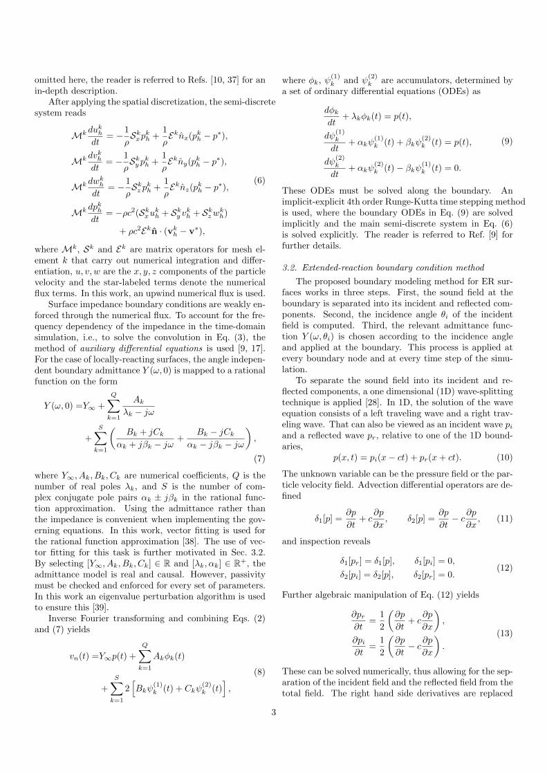
omitted here, the reader is referred to Refs. [10, 37] for anin-depth description.
After applying the spatial discretization, the semi-discretesystem reads
Mk dukh
dt= −1
ρSkxpkh +
1
ρEknx(pkh − p∗),
Mk dvkh
dt= −1
ρSky pkh +
1
ρEkny(pkh − p∗),
Mk dwkh
dt= −1
ρSkz pkh +
1
ρEknz(pkh − p∗),
Mk dpkh
dt= −ρc2(Skxukh + Sky vkh + Skzwk
h)
+ ρc2Ekn · (vkh − v∗),
(6)
where Mk, Sk and Ek are matrix operators for mesh el-ement k that carry out numerical integration and differ-entiation, u, v, w are the x, y, z components of the particlevelocity and the star-labeled terms denote the numericalflux terms. In this work, an upwind numerical flux is used.
Surface impedance boundary conditions are weakly en-forced through the numerical flux. To account for the fre-quency dependency of the impedance in the time-domainsimulation, i.e., to solve the convolution in Eq. (3), themethod of auxiliary differential equations is used [9, 17].For the case of locally-reacting surfaces, the angle indepen-dent boundary admittance Y (ω, 0) is mapped to a rationalfunction on the form
Y (ω, 0) =Y∞ +
Q∑
k=1
Ak
λk − jω
+
S∑
k=1
(Bk + jCk
αk + jβk − jω+
Bk − jCk
αk − jβk − jω
),
(7)
where Y∞, Ak, Bk, Ck are numerical coefficients, Q is thenumber of real poles λk, and S is the number of com-plex conjugate pole pairs αk ± jβk in the rational func-tion approximation. Using the admittance rather thanthe impedance is convenient when implementing the gov-erning equations. In this work, vector fitting is used forthe rational function approximation [38]. The use of vec-tor fitting for this task is further motivated in Sec. 3.2.By selecting [Y∞, Ak, Bk, Ck] ∈ R and [λk, αk] ∈ R+, theadmittance model is real and causal. However, passivitymust be checked and enforced for every set of parameters.In this work an eigenvalue perturbation algorithm is usedto ensure this [39].
Inverse Fourier transforming and combining Eqs. (2)and (7) yields
vn(t) =Y∞p(t) +
Q∑
k=1
Akφk(t)
+S∑
k=1
2[Bkψ
(1)k (t) + Ckψ
(2)k (t)
],
(8)
where φk, ψ(1)k and ψ
(2)k are accumulators, determined by
a set of ordinary differential equations (ODEs) as
dφkdt
+ λkφk(t) = p(t),
dψ(1)k
dt+ αkψ
(1)k (t) + βkψ
(2)k (t) = p(t),
dψ(2)k
dt+ αkψ
(2)k (t)− βkψ(1)
k (t) = 0.
(9)
These ODEs must be solved along the boundary. Animplicit-explicit 4th order Runge-Kutta time stepping methodis used, where the boundary ODEs in Eq. (9) are solvedimplicitly and the main semi-discrete system in Eq. (6)is solved explicitly. The reader is referred to Ref. [9] forfurther details.
3.2. Extended-reaction boundary condition method
The proposed boundary modeling method for ER sur-faces works in three steps. First, the sound field at theboundary is separated into its incident and reflected com-ponents. Second, the incidence angle θi of the incidentfield is computed. Third, the relevant admittance func-tion Y (ω, θi) is chosen according to the incidence angleand applied at the boundary. This process is applied atevery boundary node and at every time step of the simu-lation.
To separate the sound field into its incident and re-flected components, a one dimensional (1D) wave-splittingtechnique is applied [28]. In 1D, the solution of the waveequation consists of a left traveling wave and a right trav-eling wave. That can also be viewed as an incident wave piand a reflected wave pr, relative to one of the 1D bound-aries,
p(x, t) = pi(x− ct) + pr(x+ ct). (10)
The unknown variable can be the pressure field or the par-ticle velocity field. Advection differential operators are de-fined
δ1[p] =∂p
∂t+ c
∂p
∂x, δ2[p] =
∂p
∂t− c ∂p
∂x, (11)
and inspection reveals
δ1[pr] = δ1[p], δ1[pi] = 0,
δ2[pi] = δ2[p], δ2[pr] = 0.(12)
Further algebraic manipulation of Eq. (12) yields
∂pr∂t
=1
2
(∂p
∂t+ c
∂p
∂x
),
∂pi∂t
=1
2
(∂p
∂t− c ∂p
∂x
).
(13)
These can be solved numerically, thus allowing for the sep-aration of the incident field and the reflected field from thetotal field. The right hand side derivatives are replaced
3

with centered second-order finite differences, and the re-maining ODEs are solved with a Crank-Nicolson scheme.The finite difference nodes are placed along a 1D line de-fined by the boundary normal in the three dimensional(3D) space, for every boundary node. The field valuesin the finite difference nodes are computed using inter-polation. Figure 1 illustrates the setup. An example ofa separated 3D wave is shown in Fig. 2, where a spher-ical wave impinges on a flat boundary with θi = 37.6
incidence angle at the observation point on the boundary.The boundary condition is frequency independent with anormal incidence absorption coefficient of α0 = 0.5. Notethe decreased amplitude of the reflected wave, comparedto the incident wave. Furthermore, observe the change insign in the x velocity component.
Figure 1: An illustration of the sound field separation setup. Thegray dashed lines illustrate the DGFEM mesh elements and the greycircles are the DGFEM mesh nodes. The finite difference wave-splitting nodes are placed in front of every boundary DGFEM nodein a line along the boundary normal, illustrated as red stars.
0 1 2 3 4 5 6 7
10-3
-0.05
0
0.05
0 1 2 3 4 5 6 7
10-3
-1
0
110-4
Figure 2: Example of a sound field separation at a boundary of a3D domain. The domain is a rectangular 3D room (Lx, Ly , Lz) =(3, 10, 5) m. The source is located at (sx, sy , sz) = (1, 2, 2) m andthe observation point is located at (rx, ry , rz) = (0, 2.577, 2.5) m.
The wave splitting is applied to the particle velocityu, v, w components. Once the sound field has been sepa-
rated, the incidence angle is computed with
θi = arccos
(vi · n|vi||n|
), (14)
where vi = [ui vi wi]T is the incident particle velocity. In
this work, the boundary admittance is mapped to rationalfunctions with one degree angular resolution, resulting in atotal of 91 admittance functions for a given room surface.Once the angle of the incident wave is determined, thealgorithm selects the admittance function closest to thedetected angle.
When doing the rational function approximation foreach of the 91 admittance functions, care must be takento ensure that the distribution of real versus complex con-jugate poles in the rational functions is the same for allangles. While this can result in suboptimal curve fitting,i.e., a higher number of poles is required, it ensures that thesame ODEs in Eq. (9) are solved at every time step. This isdesirable because the solution of the ODEs at time step nrequires knowledge of the solution at timestep n−1. Thus,the only parameters that change in the simulation, as theincidence angle varies and a new admittance function ischosen, are the Y∞, Ak, Bk and Ck in Eq. (8). Vector fit-ting is suitable for this type of function approximation,as the real versus complex pole distribution can be keptconsistent across all incidence angles [38].
4. Angle detection accuracy analysis
Since the wave splitting is computed along a 1D line,defined by the boundary normal in 3D space, the accu-racy of the proposed separation method will vary with theincidence angle. When a wave is traveling close to nor-mal incidence, the energy flow is more or less along theboundary normal and high accuracy in the separation andangle computation should be expected. However, as theincidence angle approaches grazing incidence, the energyflow is only partially along the boundary normal, and a de-crease in accuracy should be expected. A two dimensional(2D) test case, using a plane wave incidence, is consideredto analyze the angle detection accuracy as a function ofthe incidence angle. A rectangular domain is used, wherethe left-right boundaries are made to be periodic. Thebottom boundary is the boundary of interest, where thewave splitting and angle detection are performed. The topboundary is an absorbing layer. The width of the domainis adjusted according to the incidence angle to ensure pe-riodicity. The plane wave incidence is produced using ascattered field formulation [40]. The 2D incident planewave solution is
pi = exp(j(k · x− ωt)),
vi =1
ρck exp(j(k · x− ωt)), (15)
where k = kk = k[cos θi sin θi]T is the wave vector, with
k = ω/c. In the scattered field formulation, the total field
4

solution of Eq. (1) is expressed as a superposition of theincident field and the scattered field
v = vi + vs, p = pi + ps. (16)
Inserting this into Eq. (1) yields
(vs)t = −1
ρ∇ps − γ(y)vs,
(ps)t = −ρc2∇ · vs − γ(y)ps,
(17)
since (vi, pi) satisfies Eq. (1). This system is solved usingthe wave-based scheme with (vs, ps) = 0 at t = 0 and witha frequency independent boundary condition at the bot-tom boundary, which induces the scattered field reflection
n · vs =pi + psZs
− n · vi. (18)
The terms with the γ function in Eq. (17) are added toimplement the absorbing layer at the top boundary byusing
γ(y) =
0 y ≤ Ly − a,(y−(Ly−a))q
∆t Ly − a ≤ y ≤ Ly,(19)
where a is the width of the absorbing layer, q is a numericalparameter that dictates how strongly the wave is dampedas it enters the absorbing layer, and Ly is the length ofthe domain in the y dimension. The parameters a and qmust be tuned to ensure sufficient absorption at the topboundary. In this work, setting q = 4 and following acommon rule of thumb of having the layer width be atleast two wavelengths yields satisfactory performance ofthe absorbing layer [41].
The sound field separation and subsequent angle de-tection accuracy are tested for three boundary conditions,having frequency independent normal incidence absorp-tion coefficients of α0 = 0.1, 0.5, 0.9. The results areshown in Fig. 3. The angle detection error is defined as|θe − θi|, where θe is the time averaged estimated angleand θi is the true angle of incidence of the plane wave.As expected, the angle detection error is very low for alltested boundary conditions for small incidence angles, atless than 5 for incidence angles smaller than 30. As theincidence angle increases, the error increases, however, forall cases it is less than 15. The error is larger for lessabsorbing surfaces, because here the reflected field is moreprominent. For the highly absorptive case, the error isless than 5 for incidence angles up to 70. Table 1 showsthe mean error and the maximum error for the differentabsorption conditions.
5. Single reflection validation study
In this validation study, the transfer function (TF) be-tween a source and a receiver in the presence of a sin-gle flat surface is investigated. This corresponds to a
0 10 20 30 40 50 60 70 80 900
5
10
15
Figure 3: Accuracy of the proposed sound field separation and sub-sequent angle detection procedure for a plane wave incidence.
Abs. coeff. α0 Mean error Max error0.1 6.9% 14.3%0.5 4.0% 8.7%0.9 3.0% 15.9%
Table 1: Angle detection accuracy for a plane wave incidence.
typical condition in outdoor sound propagation. Simu-lated transfer functions are compared against an analyticsolution [42] and against measurements done in an ane-choic chamber. The position of the receiver is varied totest a wide range of different incidence angles, rangingfrom θi = 12 to θi = 70. Figure 4 shows a schematicof the setup. Three porous absorbers are considered forthe boundary conditions, their specifications are given inTab. 2. They are selected to exhibit ER behavior, but to avarying degree, where A3 has the strongest ER behavior,i.e., the impedance varies strongly with incidence angle.Using porous absorbers is convenient because there existwell-established models to estimate their angle dependentsurface admittance. In this work, Miki’s model [43] anda transfer matrix method [44] is used. The admittancefunctions are mapped to rational functions using 1 angu-lar resolution. In total 14 poles are used in the functionapproximation, which gives a good approximation of theadmittance functions.
Figure 4: Single reflection validation study setup.
5

Mat. thick. Air cav. depth Flow res.ID dmat [m] d0 [m] σmat [Ns/m4]A1 0.05 0 3, 000A2 0.05 0.15 14, 400A3 0.02 0.2 50, 000
Table 2: Porous absorber configurations used.
ID Pos. [m] θi ID Pos. [m] θiS (0.75, 5.50, 5.00) - R5 (0.75, 7.90, 5.00) 58
R1 (0.75, 5.82, 5.00) 12 R6 (0.75, 8.10, 5.00) 60
R2 (1.20, 7.45, 5.00) 45 R7 (0.40, 7.97, 5.00) 65
R3 (1.20, 7.82, 5.00) 50 R8 (0.20, 7.85, 5.00) 68
R4 (0.75, 7.64, 5.00) 55 R9 (0.20, 8.11, 5.00) 70
Table 3: Source (S) and receiver (R) positions used in the singlereflection validation study.
5.1. Analytic validation
In the simulation, a 8 m × 14 m × 10 m room is usedto ensure no parasitic reflections. The domain is meshedusing tetrahedral elements with roughly 8 points per wave-length at 600 Hz, the highest frequency of interest. N = 4basis functions are used. The source and receiver positionsused in the simulation are shown in Tab. 3. The porousabsorber surface is the Y Z plane at x = 0. The source isa Gaussian pulse pressure initial condition
p(x, 0) = exp
(− (x− xs)2 + (y − ys)2 + (z − zs)2
sxyz
)
(20)where (xs, ys, zs) is the source position and sxyz = 0.15m2 is the spatial variance, which governs the frequencycontent of the pulse. The boundary condition is simu-lated using either the LR assumption or the proposed ERmethod.
Figure 5 shows simulated TFs for receiver R7, i.e., forθi = 65, for the three different porous absorbers. Inall cases, the ER method results in a considerably bet-ter agreement with the analytic solution, compared to us-ing the LR assumption. The differences between the ana-lytic solution and ER results are explained by the error inthe angle estimation. The ER method performs best forA1, because for this absorber the admittance varies mostsmoothly with incidence angle, and hence it is less sensi-tive to the accuracy of the angle detection method. ForA3, there are noticeable differences between the ER simu-lation and the analytic solution, due to the rapid variationin the surface admittance as a function of angle, making itmore sensitive to the angle detection errors. Nevertheless,the proposed method clearly outperforms the LR approachfor this case.
Figure 6 shows the mean transfer function error forall considered incidence angles. The trend is the samefor the three different absorbers: For low incidence anglesthe accuracy is comparable between using LR and the ER
150 200 250 300 350 400 450 500 550 600-40
-20
0
150 200 250 300 350 400 450 500 550 600-15
-10
-5
0
150 200 250 300 350 400 450 500 550 600-15
-10
-5
0
LRERAnalytic
Figure 5: Transfer functions for the θi = 65 incidence angle com-pared against the analytic solution. a) A1. b) A2. c) A3.
method, but for the high incidence angles, the ER methodresults in considerably lower errors.
10 20 30 40 50 60 700
2
4
6
8
10 20 30 40 50 60 700
2
4
6
8
10 20 30 40 50 60 700
2
4
6
8LRER
Figure 6: Mean transfer function error between simulation and theanalytic solution, for all incidence angles considered. a) A1. b) A2.c) A3.
5.2. Experimental validation
In this part, only absorber A2 is considered. The mea-surements are carried out in a large anechoic chamber ofaround 1000 m3. The chamber has a lower limiting fre-quency of approximately 50 Hz. The rigid backing is real-ized by a 3 cm thick wooden panel which is placed on themesh floor. The size of the absorbing sample is 10.8 m2,with dimensions 3 m× 3.6 m. The air cavity mounting is atype E mounting configuration according to ISO 354 [45].The flow resistivity of the porous material sample is mea-sured in an impedance tube, using the method suggestedby Ren et al. [46] and found to be σmat = 14 400 Ns/m4.
6

An omni-directional sound source of type B&K 4295 anda 1
2 inch microphone of type B&K 4192 is used (Bruel& Kjær, Nærum, Denmark). The source signal is an ex-ponential sine sweep. For the measurement, a two-stepprocedure suggested by Suh et al. [26] is used, where acorrection for the source spectrum and the source-receiverdistance is done. Additional details regarding the mea-surements can be found in Ref. [47].
Figure 7 shows transfer functions for selected incidenceangles. As before, there is very little difference betweenusing LR and the ER method for small incidence angles.For the larger incidence angles, the ER method matchesthe measured transfer functions considerably better.
150 200 250 300 350 400 450 500 550 600-15
-10
-5
0
LRERMeas.
150 200 250 300 350 400 450 500 550 600-15
-10
-5
0
150 200 250 300 350 400 450 500 550 600-15
-10
-5
0
Figure 7: Transfer functions for A2 for selected incidence anglescompared against measurement data. a) θi = 12. b) θi = 55. c)θi = 65.
Finally, Fig. 8 shows the mean transfer function errorfor all considered incidence angles. The trend is similar tothe results comparing simulations and the analytic solu-tion in Fig. 6b. The performance of the LR and the ERmethod is similar for small incidence angles, but for thelarger angles, the ER method is superior.
10 20 30 40 50 60 700
2
4
6LRER
Figure 8: Mean transfer function error between simulation and mea-surements, for all incidence angles considered.
6. Discussion
The results of the single reflection validation studiesshow that the simulation accuracy improves when usingthe proposed ER method, as compared to using the LRassumption. This confirms the method’s ability to capture
the angular dependence of the surface impedance, at leastfor the porous absorbers considered in this study. As afuture work, it would be interesting to investigate the per-formance of the proposed method for modeling differentsurface types, e.g., vibrating airtight panels or perforatedpanels.
A potential improvement of the proposed method couldbe to use more advanced methods for the wave splitting, toimprove the angle estimation. Such methods would likelyinclude non-local spatial derivatives in two or three dimen-sions. Different experimental and numerical approachesare described in the literature, e.g., Refs. [28, 48, 49, 50].This would, however, increase the computational cost. Itis also of great interest whether an improved detection ofthe incidence angle results in perceptually noticeable im-provements in simulation accuracy.
When comparing simulations against measurements,there are always uncertainties involved. While steps havebeen taken to minimize the uncertainties, there are somenoticeable fluctuations in the measured transfer functionsthat are likely caused by edge diffraction effects, due tothe finite sample size. Other sources of uncertainty in-clude sound source imperfections, material mounting andmaterial uniformity. Nonetheless, the experimental studydoes confirm the improved accuracy of the ER methodover using LR, as seen in Figs. 7 and 8.
As the suggested method relies on the wave splittingtechnique, the method becomes less reliable when reflec-tions begin to overlap in time. In environmental acoustics,this is generally not of concern due to the large domainsand few reflections involved. In rooms, the theoretical re-flection density follows dN
dt = 4πc3t2/V . This means thatfor larger spaces, the number of wave fronts impinging onthe boundary surfaces remains low for the early portion ofthe impulse response. One can define an average temporalspacing between reflections, which is the reciprocal of thereflection density, ∆trefl = V/4πc3t2 [51]. The proposedmethod will produce reliable results as long as the tempo-ral spacing between reflections is larger than the duration(or “temporal width”) ∆tw of the propagating pulse. Asimple way to define the pulse width is the full width athalf maximum approach [52].
Figure 9 shows the average temporal spacing ∆trefl asa function of reflection order, for three different emptyrooms. The rooms all have dimension ratios 1:1:1. Thisis then compared against the temporal widths ∆tw of twodifferent Gaussian pulses. The chosen temporal widthscorrespond to having sxyz = 0.1 m2 for the ∆tw = 0.79ms case and sxyz = 0.02 m2 for the ∆tw = 0.15 ms case.The sxyz = 0.1 m2 pulse has an upper −3 dB cutoff fre-quency of roughly 1500 Hz and the sxyz = 0.02 m2 has anupper −3 dB cutoff frequency of roughly 7500 Hz. Thefigure reveals that for all rooms considered, the methodcan be used for modeling the first few reflection orders.Table 4 shows further analysis of the results in Fig. 9.For the smallest room, and using the low-mid frequencysource condition (sxyz = 0.1 m2), the first 2.6 reflection or-
7

1 2 3 4 5 6 7 8 9 10
10-4
10-3
10-2
Figure 9: Average temporal spacing between reflections for differentrooms compared against different pulse widths of the propagatingGaussian pulse.
∆tw = 0.79 ms ∆tw = 0.15 mssxyz = 0.1 m2 sxyz = 0.02 m2
V [m3] ro Nr t [s] ro Nr t [s]1,000 2.6 21.7 0.05 5.9 253.5 0.115,000 3.4 48.6 0.11 7.7 564.8 0.2620,000 4.2 92.2 0.22 9.7 1135.4 0.51
Table 4: Reflection orders ro, number of reflections Nr and simula-tion time t that is reliable to simulate with the ER method for thedifferent rooms considered, for two different initial conditions.
ders can be included, corresponding to modeling roughlythe first 22 reflections in the room, or the first 50 ms ofthe impulse response. As the room size increases, morereflection orders can be reliably included. For the biggestroom, the first 4.2 reflection orders can be modeled withthe method, for the low-mid frequency source condition,i.e., the first 220 ms. As the pulse width decreases (morebroadband simulations), more reflection orders can be in-cluded. For the broadband source condition (sxyz = 0.02m2), the first 9.7 reflection orders can be included in thebig room simulation, corresponding to the first 510 ms ofthe impulse response.
The proposed ER method is found to add very littleadditional computational cost to the simulations. The av-erage computation time for the single reflection studiesusing the LR boundary condition is 29.90 s (0.049 s stan-dard deviation), but for the ER boundary condition it is30.54 s (0.005 s standard deviation). This corresponds to acost increase of 2.1%. The simulations are run on a singleNvidia Tesla V100 GPU. The added computational costwill be case dependent to some degree, e.g., dependingon how many surfaces are modeled with the ER method.However, the cost increase will be fairly independent ofthe complexity or physical behavior of the boundary, aschanging the surface impedance only results in changingthe numerical coefficients in the ADE method. The onlypotential cost increase would be if more poles are neededin the material mapping. In this study a high number ofpoles is used to guarantee high precision in the materialmapping. This is in contrast to boundary modeling meth-ods that model the sound propagation inside the boundarysurface. The cost of these methods is highly dependent on
the complexity and geometric features of the boundary.
7. Conclusion
A general method for modeling extended-reaction bound-aries under sparse sound field conditions, e.g., outdoorsound propagation and early reflections in large rooms,has been presented. The method relies on a wave split-ting technique, which separates the sound field in frontof a boundary into its incident and reflected components.The angle of the incident sound field is determined fromthe local particle velocity and the boundary conditions areadjusted according to the incidence angle.
The accuracy of the method is validated both analyti-cally and experimentally in a single reflection study usingdifferent porous absorbers. In all cases, an improvement inaccuracy is clearly seen when using the proposed method,as compared to the local-reaction modeling method. Theimprovement is particularly noticeable at large incidenceangles. It is also shown that the reflection density inmedium to large rooms is low enough for the method tobe able to reliably simulate the first few reflection orders.
Acknowledgments
This research has been partially funded by the Innova-tion foundation and the Realdania foundation in Denmark.The infrastructure at the Technical University of DenmarkComputing Center has been used for running simulations.
References
[1] M. Hornikx, R. Waxler, J. Forssen, The extended Fourier pseu-dospectral time-domain method for atmospheric sound propa-gation, J. Acoust. Soc. Am. 128 (4) (2010) 1632–1646.
[2] T. V. Renterghem, The finite-difference time-domain methodfor simulation of sound propagation in a moving medium, Ph.D.thesis, Ghent University, Belgium (2003).
[3] D. Hothersall, K. Horoshenkov, S. Mercy, Numerical modellingof the sound field near a tall building with balconies near a road,J. Sound Vib. 198 (4) (1996) 507–515.
[4] A. Pelat, S. Felix, V. Pagneux, A coupled modal-finite elementmethod for the wave propagation modeling in irregular openwaveguides, J. Acoust. Soc. Am. 129 (3) (2011) 1240–1249.
[5] D. Botteldooren, Finite-difference time-domain simulation oflow-frequency room acoustic problems, J. Acoust. Soc. Am.98 (6) (1995) 3302–3308.
[6] A. Craggs, A finite element method for free vibration of air inducts and rooms with absorbing walls, J. Sound Vib. 173 (1994)568–576.
[7] J. A. Hargreaves, L. R. Rendell, Y. W. Lam, A framework forauralization of boundary element method simulations includ-ing source and receiver directivity, J. Acoust. Soc. Am. 145 (4)(2019) 2625–2637.
[8] S. Bilbao, Modeling of complex geometries and boundary condi-tions in finite difference/finite volume time domain room acous-tics simulation, IEEE Trans. Audio, Speech, Lang. Proc. 21 (7)(2013) 1524–1533.
[9] F. Pind, A. P. Engsig-Karup, C. H. Jeong, J. S. Hesthaven, M. S.Mejling, J. Stromann-Andersen, Time domain room acousticsimulations using the spectral element method, J. Acoust. Soc.Am. 145 (6) (2019) 3299–3310.
8

[10] H. Wang, I. Sihar, R. P. Munoz, M. Hornikx, Room acous-tics modelling in the time-domain with the nodal discontinuousGalerkin method, J. Acoust. Soc. Am. 145 (4) (2019) 2650–2663.
[11] M. Vorlander, Computer simulations in room acoustics: Con-cepts and uncertainties, J. Acoust. Soc. Am. 133 (3) (2013)1203–1213.
[12] C. H. Jeong, G. Marbjerg, J. Brunskog, Uncertainty of inputdata for room acoustic simulations, in: Proc. Baltic-NordicAcoust. Meet., 2016.
[13] M. Hornikx, Ten questions concerning computational urbanacoustics, Build. Environm. 106 (2016) 409–421.
[14] H. Kuttruff, Room Acoustics, 5th Edition, Taylor & Francis,2009, ch. 2.
[15] M. Hodgson, A. Wareing, Comparisons of predicted steady-state levels in rooms with extended- and local-reaction boundingsurfaces, J. Sound Vib. 309 (1) (2008) 167–177.
[16] B. Yousefzadeh, M. Hodgson, Energy- and wave-based beam-tracing prediction of room-acoustical parameters using differentboundary conditions, J. Acoust. Soc. Am. 132 (3) (2012) 1450–1461.
[17] D. Dragna, P. Pineau, P. Blanc-Benon, A generalized recursiveconvolution method for time-domain propagation in porous me-dia, J. Acoust. Soc. Am. 138 (2) (2015) 1030–1042.
[18] A. Southern, S. Siltanen, D. T. Murphy, L. Savioja, Room im-pulse response synthesis and validation using a hybrid acousticmodel, IEEE Trans. Audio, Speech, Lang. Proc. 21 (9) (2013)1940–1952.
[19] H. Wang, M. Hornikx, Time-domain impedance boundary con-dition modeling with the discontinuous Galerkin method forroom acoustics simulations, J. Acoust. Soc. Am. 147 (4) (2020)2534–2546.
[20] S. Bilbao, B. Hamilton, J. Botts, L. Savioja, Finite volume timedomain room acoustics simulation under general impedanceboundary conditions, IEEE Trans. Audio, Speech, Lang. Proc.24 (1) (2016) 161–173.
[21] J. Zhao, M. Bao, X. Wang, H. Lee, S. Sakamoto, An equiva-lent fluid model based finite-difference time-domain algorithmfor sound propagation in porous material with rigid frame, J.Acoust. Soc. Am. 143 (1) (2018) 130–138.
[22] J. Zhao, Z. Chen, M. Bao, H. Lee, S. Sakamoto, Two-dimensional finite-difference time-domain analysis of soundpropagation in rigid-frame porous material based on equivalentfluid model, Appl. Acoust. 146 (2019) 204–212.
[23] T. Okuzono, N. Shimizu, K. Sakagami, Predicting absorptioncharacteristics of single-leaf permeable membrane absorbers us-ing finite element method in a time domain, Appl. Acoust. 151(2019) 172–182.
[24] G. Marbjerg, J. Brunskog, C.-H. Jeong, E. Nilsson, Develop-ment and validation of a combined phased acoustical radiosityand image source model for predicting sound fields in rooms, J.Acoust. Soc. Am. 138 (3) (2015) 1457–1468.
[25] A. Wareing, M. Hodgson, Beam-tracing model for predictingsound fields in rooms with multilayer bounding surfaces, J.Acoust. Soc. Am. 118 (4) (2005) 2321–2331.
[26] J. S. Suh, P. A. Nelson, Measurement of transient responseof rooms and comparison with geometrical acoustic models, J.Acoust. Soc. Am. 105 (4) (1999) 2304–2317.
[27] Y. W. Lam, Issues for computer modelling of room acousticsin non-concert hall settings, Acoust. Sci. Tech. 26 (2) (2005)145–155.
[28] M. J. Grote, M. K., F. Nataf, F. Assous, Time-dependent wavesplitting and source separation, J. Comput. Phys. 330 (2017)981–996.
[29] H. de Bree, R. Lanoye, S. de Cock, J. van Heck, In situ, broadband method to determine the normal and oblique reflectioncoefficient of acoustic materials, in: Proc. Noise. Vib. Conf.,2005.
[30] J. Ducourneau, V. Planeau, J. Chatillon, A. Nejade, Measure-ment of sound absorption coefficients of flat surfaces in a work-shop, Appl. Acoust. 70 (2009) 710–721.
[31] A. Richard, E. Fernandez-Grande, J. Brunskog, C.-H. Jeong,
Estimation of surface impedance at oblique incidence based onsparse array processing, J. Acoust. Soc. Am. 141 (6) (2017)4115–4125.
[32] M. Nolan, Estimation of angle-dependent absorption coefficientsfrom spatially distributed in situ measurements, J. Acoust. Soc.Am. 147 (2) (2020) EL119–EL124.
[33] J. S. Bradley, H. Sato, M. Picard, On the importance of earlyreflections for speech in rooms, J. Acoust. Soc. Am. 113 (6)(2003) 3233–3244.
[34] W. M. Hartmann, Localization of sound in rooms, J. Acoust.Soc. Am. 74 (5) (1983) 1380–1391.
[35] M. Vorlaender, D. Schroder, S. Pelzer, F. Wefers, Virtual realityfor architectural acoustics, J. Build. Perf. Sim. 8 (2015) 15–25.
[36] C.-H. Jeong, Guideline for adopting the local reaction assump-tion for porous absorbers in terms of random incidence absorp-tion coefficients, Acta Acust. Acust. 97 (5) (2011) 779–790.
[37] J. S. Hesthaven, T. Warburton, Nodal Discontinuous GalerkinMethods—Algorithms, Analysis, and Applications, Springer,New York, 2008, ch. 3.
[38] B. Gustavsen, A. Semlyen, Rational approximation of frequencydomain responses by vector fitting, IEEE Trans. Pow. Del.14 (3) (1999) 1052–1061.
[39] B. Gustavsen, Fast passivity enforcement for pole-residue mod-els by perturbation of residue matrix eigenvalues, IEEE Trans.Pow. Del. 23 (4) (2008) 2278–2285.
[40] D. E. Merewether, R. G. Fisher, F. W. Smith, On implementinga numeric Huygen’s source scheme in a finite difference programto illuminate scattering bodies, IEEE Trans. on Nucl. Sci. 27(1980) 1829–1833.
[41] A. P. Engsig-Karup, S. Glimberg, A. Nielsen, O. Lindberg,Fast hydrodynamics on heterogeneous many-core hardware, in:R. Couturier (Ed.), Designing Scientific Applications on GPUs,CRC Press / Taylor & Francis Group, Boca Raton, 2013, pp.251–294.
[42] S.-I. Thomasson, Reflection of waves from a point source by animpedance boundary, J. Acoust. Soc. Am. 59 (4) (1976) 780–785.
[43] Y. Miki, Acoustical properties of porous materials—modifications of Delany-Bazley models, J. Acoust. Soc.Jap. 11 (1) (1990) 19–24.
[44] J. F. Allard, N. Atalla, Propagation of Sound in Porous Media:Modelling sound absorbing materials, 3rd Edition, Wiley, WestSussex, United Kingdom, 2009, ch. 3.
[45] ISO 354, Acoustics—Measurement of sound absorption in a re-verberation room, International organization for standardiza-tion (2003).
[46] M. Ren, F. Jacobsen, A method of measuring the dynamicflow resistance and reactance of porous materials, Appl. Acoust.39 (4) (1993) 265–276.
[47] K. Gunnarsdottir, C.-H. Jeong, G. Marbjerg, Acoustic behaviorof porous ceiling absorbers based on local and extended reaction,J. Acoust. Soc. Am. 137 (1) (2015) 509–512.
[48] E. Fernandez-Grande, F. Jacobsen, Q. Leclere, Sound field sepa-ration with sound pressure and particle velocity measurements,J. Acoust. Soc. Am. 132 (6) (2012) 3818–3825.
[49] C. Langrenne, M. Melon, A. Garcia, Boundary element methodfor the acoustic characterization of a machine in bounded noisyenvironment, J. Acoust. Soc. Am. 121 (5) (2007) 2750–2757.
[50] G. Ducrozet, A. P. Engsig-Karup, H. B. Bingham, P. Fer-rant, A non-linear wave decomposition model for efficientwave–structure interaction. Part A: Formulation, validationsand analysis, J.Comput. Phys. 257 (2014) 863–883.
[51] C.-H. Jeong, J. Brunskog, F. Jacobsen, Room acoustic tran-sition time based on reflection overlap, J. Acoust. Soc. Am.127 (5) (2010) 2733–2736.
[52] R. B. Standler, Protection of Electronic Circuits from Overvolt-ages, Wiley-Interscience, New York, 2002, p. 84.
9

PAPER P4
103

Time-domain room acoustic simulations withextended-reacting porous absorbers using thediscontinuous Galerkin method
Finnur Pind,1, a) Cheol-Ho Jeong,2 Allan P. Engsig-Karup,3 Jan S. Hesthaven,4 and Jakob Strømann-Andersen1
1Henning Larsen, Copenhagen, Denmark2Acoustic Technology, Department of Electrical Engineering, Technical University of Denmark,
Kongens Lyngby, Denmark3Scientific Computing, Department of Applied Mathematics and Computer Science, Technical Uni-
versity of Denmark, Kongens Lyngby, Denmark4Chair of Computational Mathematics and Simulation Science, Ecole polytechnique federale de Lau-
sanne, Lausanne, Switzerland
This paper presents an equivalent fluid model (EFM) formulation in a 3D time-domain dis-continuous Galerkin finite element method framework for room acoustic simulations. Usingthe EFM allows for the modeling of the extended-reaction (ER) behavior of porous soundabsorbers. The EFM is formulated in the numerical framework by using the method ofauxiliary differential equations to account for the frequency dependent dissipation of theporous material. The formulation is validated analytically and an excellent agreement withthe theory is found. Experimental validation for a single reflection case is also conducted,and it is shown that using the EFM improves the simulation accuracy when modeling aporous material backed by an air cavity, as compared to using the local-reaction (LR) ap-proximation. Lastly, a comparative study of different rooms with different porous absorbersis presented, using different boundary modeling techniques, namely, a LR approximation, afield-incidence (FI) approximation, or modeling the full ER behavior with the EFM. It isshown that using a LR or FI approximation leads to large and perceptually noticeable errorsin simulated room acoustic parameters. The average T20 reverberation time error is 3.8 timesthe just-noticeable-difference (JND) threshold when using LR and 2.7 JND when using FI.
c©2020 Acoustical Society of America. [http://dx.doi.org(DOI number)]
[XYZ] Pages: 1–14
Keywords: Room acoustic simulations, extended-reaction boundary conditions, equivalentfluid model, time-domain discontinuous Galerkin method.
I. INTRODUCTION
The sound absorption properties of room surfaceshave a major influence on the acoustics of rooms. It istherefore important to model these properties accuratelywhen simulating room acoustics. When a sound wavehits a surface, the angle of transmission is determinedby Snell’s law of refraction. However, for certain roomsurfaces, a simpler local-reaction (LR) model can be ap-plied, where the wave is assumed to be refracted suchthat it only propagates perpendicularly to the surface.1
Hence, the frequency dependent normal incidence surfaceimpedance is a sufficient descriptor for a room surface ofthis type. In practice, however, the LR assumption isnot appropriate for most room surfaces.2 For most sur-faces, waves are refracted according to Snell’s law, effec-tively implying that surface impedance varies with the
incidence angle of the incident wave, i.e., they are said toexhibit extended-reaction (ER) behavior.
Due to their highly absorptive properties, porous ma-terials, e.g., mineral wool, glass wool and polyurethanefoams, are frequently employed in building design to con-trol the acoustics of rooms. The LR assumption is gen-erally considered acceptable for porous materials with ahigh flow resistivity and mounted on a rigid backing.3
However, for porous materials with a low flow resistiv-ity or when porous materials are backed by an air cav-ity, the LR assumption is not appropriate and insteadthe ER must be incorporated into the simulation.3–11
Sound propagation in porous materials can be describedby Biot theory, where there are three propagating waves,an elastic compression wave, an elastic shear wave andan acoustic compression wave.12 To reduce the computa-tional complexity of the full poroelastic Biot model, anequivalent fluid model (EFM) can be used, as long as thewavelength is much larger than the characteristic dimen-sions of the pores in the material.13 In the EFM, onlythe acoustic compression wave propagates and the frame
J. Acoust. Soc. Am. / 22 June 2020 1

surrounding the porous material is assumed to be eitherrigid or limp. For both frame types, the same governingequations apply, but a correction of the material’s effec-tive density is applied if the frame is taken to be limp.14
In wave-based room acoustic simulations, the govern-ing partial differential equations are solved numerically.Different numerical techniques have been employed, e.g.,the finite-difference time-domain method (FDTD),15 thefinite element method (FEM),16 the boundary elementmethod (BEM),17 the finite volume method (FVM),18
and, recently, high-order accurate methods such as thespectral element method (SEM),19 or the discontinuousGalerkin finite element method (DGFEM).20 The dis-continuous Galerkin method, which is used in this work,is particularly attractive for room acoustic simulations,due to its high-order accuracy, its geometric flexibility,its suitability for parallel computing, and its lean mem-ory usage.21 Wave-based simulations have the potentialto be highly accurate, as they inherently include all wavephenomena such as diffraction and interference. How-ever, accurate modeling of the boundary conditions isof utmost importance to achieve accurate results.22,23
Most wave-based methods discussed in the literaturetreat boundary surfaces as locally reacting, thereby ren-dering the boundary conditions somewhat of an Achillesheel of wave-based simulations. This is especially true forthe time-domain variants,19,24,25 as it is not as straight-forward to model frequency dependent propagation anddissipation in the time domain as in the frequency do-main. It is, nonetheless, desirable to model ER in time-domain simulations, because simulations in the time do-main offer certain benefits, by allowing transient analysis,time varying settings and the use of simulated impulseresponses directly for auralization purposes.
In recent years, the interest of modeling ER bound-ary conditions in wave-based simulations has seen someincrease. Aretz et al.3 described an EFM approach basedon the Zwikker and Kosten phenomenological model forporous absorbers in a frequency domain FEM. Theyalso investigated the use of a simpler field-incidence (FI)method to account for the ER, i.e., a weighted angle-averaged surface impedance. They found that in somecases the FI approach improves the simulation accuracyas compared to the LR, and is comparable to using anEFM. Tomiku et al.26 compared weighted angle-averagedimpedance versus LR models and saw some improve-ments in accuracy. Dragna et al.27 modeled sound prop-agation in a porous material in a time-domain Fourierpseudospectral simulation framework by solving the Wil-son’s model equations,28 and applied the framework tomodel outdoor sound propagation. Zhao et al.29,30 pro-posed an FDTD algorithm based on IIR filters for anEFM and applied it to 1D and 2D cases. Okuzono etal.31 presented a method to model the ER of a single-leaf permeable membrane absorber in time-domain FEMsimulations.
The contribution of this paper is threefold. Firstly,it is shown how an EFM can be formulated in a time-domain DGFEM simulation framework and used to sim-
ulate the ER behavior of porous absorbers. To the bestof the authors’ knowledge, this is the first time an EFMis used in time-domain DGFEM. A general form of thegoverning equations in the EFM is used, where the fre-quency dependent viscothermal dissipation properties aredescribed by the material’s effective density and effec-tive bulk modulus. Using this general formulation yieldscomplete freedom in selecting material models to char-acterize the material, from simple models such as theMiki model32 to more advanced models such as the JCALmodel.33 This is in contrast to using model-specific for-mulations such as Wilson’s model or the Zwikker andKosten model. Secondly, experimental validations areconducted for a single reflection case, with a porous ma-terial backed by an air cavity. Thirdly, a comparativestudy of three rooms with different porous absorbers,which are modeled using either LR, FI, or the EFM, ispresented. This study is inspired by the studies of Hodg-son et al.8,9 The purpose is to provide insights into whenit is necessary to model the full ER of porous absorbers,and when it is reasonable to use simpler methods, suchas LR or FI. The difference between the present studyand the previous studies by Hodgson et al. is that here awave-based simulation method is used, whereas they useda geometrical acoustics method. Furthermore, Hodgsonet al. only compared LR and ER, whereas in this studythe FI approach is also considered.
The paper is organized as follows. In Sec. II, thegoverning equations of sound propagation in air and inporous materials are given. Section III describes howthe governing equations are solved using the proposednumerical framework. In Sec. IV, numerical results arecompared against theory to validate the proposed formu-lation and implementation. Section V contains the exper-imental validation study. Then, in Sec. VI, the compara-tive study of the different boundary modeling techniquesis presented. Finally, some concluding remarks are of-fered in section VII.
II. GOVERNING EQUATIONS
A. In air
The following set of first order partial differentialequations describes wave motion in a lossless medium,
∂v
∂t= −1
ρ∇p,
in ΩA,∂p
∂t= −ρc2∇ · v,
(1)
where v(x, t) is the particle velocity, p(x, t) is the soundpressure, x is the position in the air domain ΩA, t is time,c is the speed of sound in air and ρ is the density of air(c = 343 m/s and ρ = 1.2 kg/m3 in this work).
2 J. Acoust. Soc. Am. / 22 June 2020
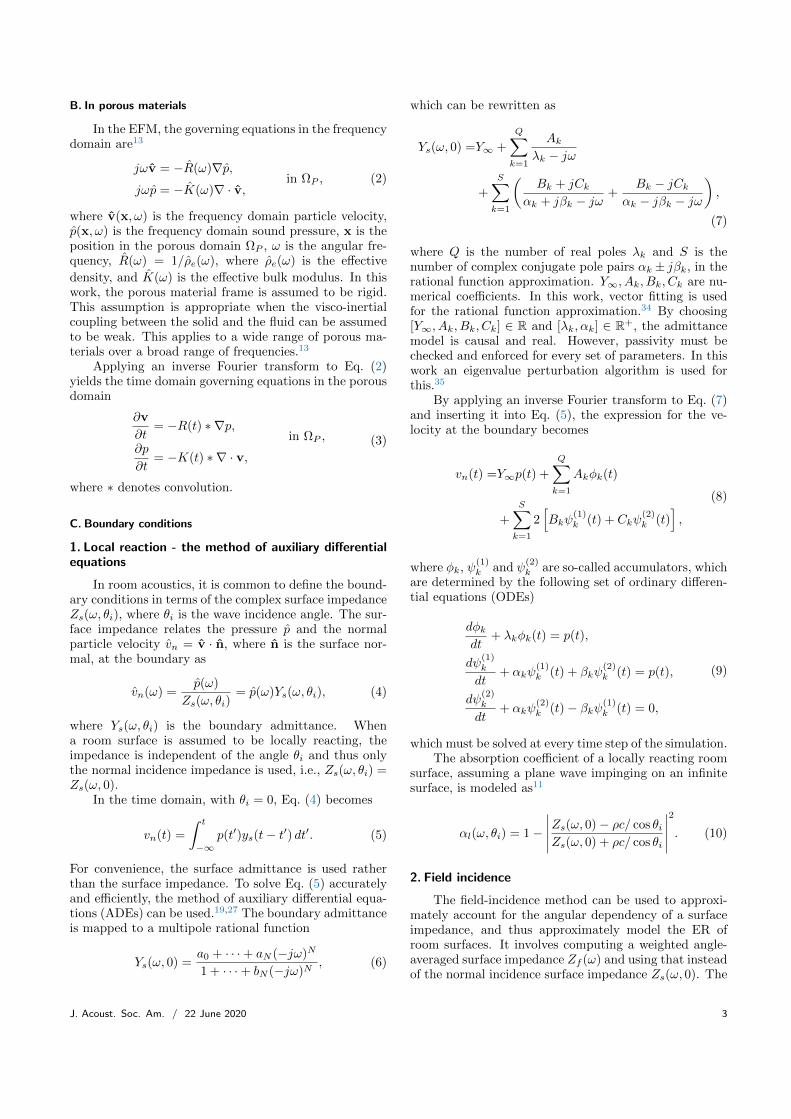
B. In porous materials
In the EFM, the governing equations in the frequencydomain are13
jωv = −R(ω)∇p,in ΩP ,
jωp = −K(ω)∇ · v,(2)
where v(x, ω) is the frequency domain particle velocity,p(x, ω) is the frequency domain sound pressure, x is theposition in the porous domain ΩP , ω is the angular fre-quency, R(ω) = 1/ρe(ω), where ρe(ω) is the effective
density, and K(ω) is the effective bulk modulus. In thiswork, the porous material frame is assumed to be rigid.This assumption is appropriate when the visco-inertialcoupling between the solid and the fluid can be assumedto be weak. This applies to a wide range of porous ma-terials over a broad range of frequencies.13
Applying an inverse Fourier transform to Eq. (2)yields the time domain governing equations in the porousdomain
∂v
∂t= −R(t) ∗ ∇p,
in ΩP ,∂p
∂t= −K(t) ∗ ∇ · v,
(3)
where ∗ denotes convolution.
C. Boundary conditions
1. Local reaction - the method of auxiliary differentialequations
In room acoustics, it is common to define the bound-ary conditions in terms of the complex surface impedanceZs(ω, θi), where θi is the wave incidence angle. The sur-face impedance relates the pressure p and the normalparticle velocity vn = v · n, where n is the surface nor-mal, at the boundary as
vn(ω) =p(ω)
Zs(ω, θi)= p(ω)Ys(ω, θi), (4)
where Ys(ω, θi) is the boundary admittance. Whena room surface is assumed to be locally reacting, theimpedance is independent of the angle θi and thus onlythe normal incidence impedance is used, i.e., Zs(ω, θi) =Zs(ω, 0).
In the time domain, with θi = 0, Eq. (4) becomes
vn(t) =
∫ t
−∞p(t′)ys(t− t′) dt′. (5)
For convenience, the surface admittance is used ratherthan the surface impedance. To solve Eq. (5) accuratelyand efficiently, the method of auxiliary differential equa-tions (ADEs) can be used.19,27 The boundary admittanceis mapped to a multipole rational function
Ys(ω, 0) =a0 + · · ·+ aN (−jω)N
1 + · · ·+ bN (−jω)N, (6)
which can be rewritten as
Ys(ω, 0) =Y∞ +
Q∑
k=1
Akλk − jω
+S∑
k=1
(Bk + jCk
αk + jβk − jω+
Bk − jCkαk − jβk − jω
),
(7)
where Q is the number of real poles λk and S is thenumber of complex conjugate pole pairs αk ± jβk, in therational function approximation. Y∞, Ak, Bk, Ck are nu-merical coefficients. In this work, vector fitting is usedfor the rational function approximation.34 By choosing[Y∞, Ak, Bk, Ck] ∈ R and [λk, αk] ∈ R+, the admittancemodel is causal and real. However, passivity must bechecked and enforced for every set of parameters. In thiswork an eigenvalue perturbation algorithm is used forthis.35
By applying an inverse Fourier transform to Eq. (7)and inserting it into Eq. (5), the expression for the ve-locity at the boundary becomes
vn(t) =Y∞p(t) +
Q∑
k=1
Akφk(t)
+
S∑
k=1
2[Bkψ
(1)k (t) + Ckψ
(2)k (t)
],
(8)
where φk, ψ(1)k and ψ
(2)k are so-called accumulators, which
are determined by the following set of ordinary differen-tial equations (ODEs)
dφkdt
+ λkφk(t) = p(t),
dψ(1)k
dt+ αkψ
(1)k (t) + βkψ
(2)k (t) = p(t),
dψ(2)k
dt+ αkψ
(2)k (t)− βkψ(1)
k (t) = 0,
(9)
which must be solved at every time step of the simulation.The absorption coefficient of a locally reacting room
surface, assuming a plane wave impinging on an infinitesurface, is modeled as11
αl(ω, θi) = 1−∣∣∣∣∣Zs(ω, 0)− ρc/ cos θiZs(ω, 0) + ρc/ cos θi
∣∣∣∣∣
2
. (10)
2. Field incidence
The field-incidence method can be used to approxi-mately account for the angular dependency of a surfaceimpedance, and thus approximately model the ER ofroom surfaces. It involves computing a weighted angle-averaged surface impedance Zf (ω) and using that insteadof the normal incidence surface impedance Zs(ω, 0). The
J. Acoust. Soc. Am. / 22 June 2020 3

FI surface impedance is given by
Yf (ω) =
∫ 78
0 Ys(ω, θi) sin θi dθi∫ 78
0 sin θi dθi, Zf (ω) =
1
Yf (ω).
(11)The choice of integration range from 0 to 78 degrees isempirically motivated.36 Thus, the resulting plane-waveabsorption coefficient becomes
αf (ω, θi) = 1−∣∣∣∣∣Zf (ω)− ρc/ cos θiZf (ω) + ρc/ cos θi
∣∣∣∣∣
2
. (12)
3. Extended reaction
For an ER surface, the absorption coefficient is mod-eled by
αe(ω, θi) = 1−∣∣∣∣∣Zs(ω, θi)− ρc/ cos θiZs(ω, θi) + ρc/ cos θi
∣∣∣∣∣
2
. (13)
In wave-based simulations, it is difficult to accuratelydetermine the incidence angle of the incident soundwave. Therefore, instead of utilizing a surface impedanceboundary condition, the sound propagation can be simu-lated inside the boundary surface, which is coupled withthe air domain simulation. This effectively captures theangular dependence, and thus the ER, of the surface.
III. NUMERICAL DISCRETIZATION
A. Spatial discretization of the air domain equations
The spatial domain ΩA is divided into a union of non-
overlapping elements Dk, i.e., ΩA ≈ (ΩA)h =⋃Kk=1D
k,where K is the total number of elements in the mesh andh denotes the approximation. In this work tetrahedralelements are used in all 3D simulations. On each element,the local solution is represented as a nodal polynomialseries expansion
vk ≈ vkh =
Np∑
m=1
vkh(xkm, t)`km(x),
pk ≈ pkh =
Np∑
m=1
pkh(xkm, t)`km(x),
(14)
where vkh(xkm, t) and pkh(xkm, t) are the unknown nodalvalues of the particle velocity and the pressure, respec-tively, `km are the nodal basis functions, taken to beLagrange polynomials of order N , and Np = (N +d)!/(N !d!), is the number basis functions (or nodes) perelement, where d is number of dimensions. The α-optimized intra-element nodal distribution is used dueto its low Lebesque constants.37 The global solution canbe computed by performing a direct sum over the localelement solutions. Moreover, the solution in an arbitraryposition in the domain can be computed to high-orderaccuracy using polynomial interpolation.
By forming a residual on each element and requiringthe residual to vanish in the Galerkin sense, the governingequations in air become
∫
Dk
(∂vkh∂t
+1
ρ∇pkh
)`kn dx = 0,
∫
Dk
(∂pkh∂t
+ ρc2∇ · vkh)`kn dx = 0.
(15)
Applying integration by parts twice gives the final strongformulation of the governing equations
∫
Dk
∂vkh∂t
`kn dx =− 1
ρ
∫
Dk
∇pkh`kn dx
+1
ρ
∫
∂Dk
n · (pkh − p∗)`kn dx,∫
Dk
∂pkh∂t
`kn dx =− ρc2∫
Dk
∇ · vkh`kn dx
+ ρc2∫
∂Dk
n · (vkh − v∗)`kn dx,
(16)
where the star-labeled terms denote the numerical fluxterms. In this work, a central numerical flux is employed,e.g., p∗ = (p−+p+)/2, where p− denotes the nodal valueat the interface within the element and p+ denotes thecorresponding value at the interface in the neighboringelement. The central flux is non-dissipative and thus thesemi-discrete discretization is energy conserving.21
Inserting Eq. (14) into the strong formulation inEq. (16) leads to the following semi-discrete system
Mk dukh
dt=− 1
ρSkxpkh +
1
ρEknx(pkh − p∗),
Mk dvkh
dt=− 1
ρSky pkh +
1
ρEkny(pkh − p∗),
Mk dwkh
dt=− 1
ρSkz pkh +
1
ρEknz(pkh − p∗),
Mk dpkh
dt=− ρc2(Skxukh + Sky vkh + Skzwkh)
+ ρc2Ekn · (vkh − v∗),
(17)
where u, v, w are the x, y, z components of the particlevelocity and the following matrix operators are defined
Mkmn =
∫
Dk
`km(x)`kn(x)dx ∈ RNp×Np ,
(Skj)mn
=
∫
Dk
`km(x)∂`kn(x)
∂xjdx ∈ RNp×Np ,
(18)
where j is the jth Cartesian coordinate. M is themass matrix and S the stiffness matrix. Furthermore,Ek ∈ RNp×4Nfp , where Nfp is the number of nodes on asingle element face, is a matrix operator for carrying outthe surface integration. For this purpose, a surface massmatrix for each element face is defined
Mkfmn =
∫
∂Dkf
`km(x)`kn(x)dx, (19)
4 J. Acoust. Soc. Am. / 22 June 2020

where f is the face index, ranging from 1 to 4 for tetrahe-dral elements. Then the first Nfp columns of Ek consistof Mk1, in the rows corresponding to the face points forface 1, the next Nfp columns consist of Mk2 and so on.For the sake of brevity, the details of how to compute theelement matrices are omitted here. The reader is referredto Ref.21 for an in-depth description.
Surface impedance boundary conditions are weaklyenforced through the numerical flux terms. For elementfaces that lie on the domain boundary, there does notexist a value at the neighboring element interface (e.g.,p+). Instead, the neighboring value is given by p+ = p−
and v+ = −v−+2gv, where n ·gv = vn, with vn given byEq. (8). Thus, at the boundary nodes, the flux term inthe pressure equation in Eq. (17) becomes n ·(vkh−v∗) =n · v− − vn.
B. Spatial discretization of the porous domain equations -
equivalent fluid model formulation
The governing equations in the porous domain,Eq. (3), are reformulated by applying the method ofADEs. Consider the velocity equation
∂v
∂t= −R(t) ∗ ∇p = −
∫ t
−∞R(t′)∇p(t− t′) dt′. (20)
Following the procedure described in Sec. II C 1, the fre-quency domain material response R(ω) is mapped to amultipole rational function, inverse Fourier transformedand inserted into Eq. (20) to recover
∂v
∂t=− R∞∇p−
QR∑
i=1
ARi φφφRi
−SR∑
i=1
2[BRi (ψψψRi )(1) + CRi (ψψψRi )(2)
],
(21)
where φφφRi , (ψψψRi )(1) and (ψψψRi )(2) are the accumulators, de-termined by
dφφφRidt
+ λRi φφφRi = ∇p,
d(ψψψRi )(1)
dt+ αRi (ψψψRi )(1) + βRi (ψψψRi )(2) = ∇p,
d(ψψψRi )(2)
dt+ αRi (ψψψRi )(2) − βRi (ψψψRi )(1) = 0.
(22)
A similar procedure is applied to the pressure equationin Eq. (3). However, due to the non-oscillatory natureof the effective bulk modulus and the effective densityfrequency responses in porous materials, the best fittingaccuracy in the multipole rational function mapping isobtained by using only real poles in the mapping. Thus,the remaining derivation and all numerical tests only em-ploy real poles. The derivation could easily be extendedto include also complex poles. The governing equations
in the porous domain become
∂v
∂t= −R∞∇p−ΨΨΨR,
∂p
∂t= −K∞∇ · v −ΨK ,
∂φφφRi∂t
= −λRi φφφRi +∇p,∂φKi∂t
= −λKi φKi +∇ · v,
(23)
where the Ψ terms can be thought of as source terms,and are given by
ΨΨΨR =
QR∑
i=1
ARi φφφRi , ΨK =
QK∑
i=1
AKi φKi . (24)
To arrive at the strong formulation of the governing equa-tions, the same procedure that is described in Sec. III Ais applied. The porous domain is discretized by a set ofnon-overlapping elements and a local residual, that is re-quired to vanish in the Galerkin sense, is formed on eachelement. Then integration by parts twice yields
∫
Dk
∂vkh∂t
`kn dx = −R∞∫
Dk
∇pkh`kn dx
−∫
Dk
(ΨΨΨR)kh`kn dx + R∞
∫
∂Dk
n · (pkh − p∗)`kn dx,∫
Dk
∂pkh∂t
`kn dx = −K∞∫
Dk
∇ · vkh`kn dx
−∫
Dk
(ΨK)kh`kn dx + K∞
∫
∂Dk
n · (vkh − v∗)`kn dx,
∫
Dk
∂(φφφRi )kh∂t
`kn dx = −λRi∫
Dk
(φφφRi )kh`kn dx
+
∫
Dk
∇pkh`kn dx +
∫
∂Dk
n · (p∗ − pkh)`kn dx,
∫
Dk
∂(φKi )kh∂t
`kn dx = −λKi∫
Dk
(φKi )kh`kn dx
+
∫
Dk
∇ · vkh`kn dx +
∫
∂Dk
n · (v∗ − vkh)`kn dx.
(25)
Inserting the finite dimensional series expansions for theunknown variables yields the following semi-discrete sys-
J. Acoust. Soc. Am. / 22 June 2020 5

tem
Mk dukh
dt= −R∞Skxpkh −Mk(ΨR
x )kh + R∞Ekn · (pkh − p∗),
Mk dvkh
dt= −R∞Sky pkh −Mk(ΨR
y )kh + R∞Ekn · (pkh − p∗),
Mk dwkh
dt= −R∞Skz pkh −Mk(ΨR
z )kh + R∞Ekn · (pkh − p∗),
Mk dpkh
dt= −K∞(Skxukh + Sky vkh + Skzwkh)
−Mk(ΨK)kh + K∞Ekn · (vkh − v∗),
Mk d[(φRi )x]khdt
= −λRi Mk[(φRi )x]kh + Skxpkh+ Ekn · (p∗ − pkh),
Mk d[(φRi )y]khdt
= −λRi Mk[(φRi )y]kh + Sky pkh+ Ekn · (p∗ − pkh),
Mk d[(φRi )z]kh
dt= −λRi Mk[(φRi )z]
kh + Skz pkh
+ Ekn · (p∗ − pkh),
Mk d(φKi )khdt
= −λKi Mk(φKi )kh + (Skxukh + Sky vkh + Skzwkh)
+ Ekn · (v∗ − vkh),(26)
where the matrix operators are defined in Eqs. (18) and(19).
When solving the coupled problem, the semi-discretesystem in Eq. (17) is solved for the air domain elementsand the semi-discrete system in Eq. (26) is solved for theporous domain elements. Note that no additional inter-facing techniques between the two domains must be in-troduced, since the solution is computed locally for eachelement and the coupling between elements is handledthrough the flux terms.
C. Temporal discretization and stability
The semi-discrete systems in Eqs. (17) and (26) canbe expressed as a general form ODE
dqhdt
= L(qh(t), t), (27)
where qh is a vector of all unknown variables and L isthe spatial operator. This ODE system is integrated intime using a low-storage 4th order explicit Runge-Kuttatime-stepping method,
q(0)h = qnh,
i ∈ [1, . . . , 5] :
k(i) = aik
(i−1) + ∆tL(q(i−1)h , tn + ci∆t),
q(i)h = q
(i−1)h + bik
(i),
qn+1h = q
(5)h ,
(28)
where ∆t = tn+1 − tn is the time step size and the coef-ficients ai, bi, ci are given in Ref.38.
Explicit time-stepping methods impose a conditionalstability criterion, ∆t ≤ C1/(max |λe|), where λe are theeigenvalues of the spatial (right hand side) discretiza-tion and C1 is a constant relating to the size of the sta-bility region of the time-stepping method.19 There aretwo mechanisms at play that influence the maximumallowed time step: 1) the eigenvalue spectrums of thematrix operators and 2) the stiffness of the ADEs. InDGFEM, the matrix operator eigenvalue spectrum scalesas max |λe| ∼ C2cN
2γ , where the C2 constant is dictatedby the size of the smallest mesh element and γ is thehighest order of differentiation in the governing equations(γ = 1, here).39 In air, c = 343 m/s, whereas in a porousmaterial EFM, the wave speed is frequency dependent,
given by cP (ω) =
√K(ω)/ρe(ω). As shown in Fig. 1, the
wave speed is lower in the porous domain than in the airdomain, and, therefore, the speed of sound in air is usedin the time step size computation. Thus, in this work,the time step size is given as
∆t = CCFL min(∆xl)1
c
1
N2, (29)
where ∆xl is the smallest edge length of the mesh ele-ments and CCFL is a constant of O(1).
102 1030
50
100
150
200
250
300
FIG. 1. (Color online) Speed of sound in a porous domain
EFM with different flow resistivities. The effective bulk mod-
ulus and effective density of the porous material are deter-
mined using the Miki model.32
No measures have been taken to automatically ad-dress the potential stiffness of the ADEs. In almost allnumerical experiments undertaken, the matrix operatoreigenvalue spectrum is found to be the dominating con-dition on the time step size. In the few cases where theADEs impose a stricter condition, the constant CCFL isdecreased until a stable system is achieved. In those fewcases, only a minor adjustment of the constant is needed.
IV. ANALYTIC VERIFICATION
A. Absorber configurations
For the remainder of this paper, three porous ab-sorbers will be used in the different experiments under-taken. Their specifications are given in Tab. I. They areselected such that they all exhibit ER behavior, but toa varying degree, where A1 has the mildest ER behav-ior and A3 has the strongest ER behavior. In all cases,the Miki model is used to estimate the characteristic
6 J. Acoust. Soc. Am. / 22 June 2020

Mat. thick. Air cav. depth Flow res.
dmat [m] d0 [m] σmat [Ns/m4]
Absorber 1 (A1) 0.1 0 3, 000
Absorber 2 (A2) 0.05 0.15 14, 400
Absorber 3 (A3) 0.02 0.2 50, 000
TABLE I. Porous absorber configurations used.
impedance Zc and the wavenumber kt.32 The effective
bulk modulus and the effective density of the porous ma-terial, needed for the EFM, are given by K = Zc/(kt/ω)
and ρe = Z2c /K, respectively.
When the porous absorbers are modeled using eitherLR or FI, the surface impedance is determined using atransfer matrix method. For a porous material, backedby another material having a surface impedance Zb, theimpedance at the surface of the porous material for aplane wave incident at θi is13
Zs(ω, θi) =Zcktkx
(−jZb cot(kxdmat) + Zc
ktkx
Zb − jZc ktkx cot(kxdmat)
), (30)
where kx =√k2t − k20 sin2 θi, with k0 being the
wavenumber in air. When the porous material isbacked by a rigid backing, i.e., Zb = ∞, Eq. (30) re-duces to Zs(ω, θi) = −jZc(kt/kx) cot(kxdmat). Whenthe porous material is backed by an air cavity, Zb =−jρc cot(k0 cos θid0)/ cos θi. In the appendix, the fre-quency and angle dependent plane-wave absorption coef-ficients of the three absorbers are shown.
B. 1D plane wave single reflection test
As a simple first validation test of the EFM formu-lation, consider a one dimensional domain that is ter-minated by one of the porous absorbers in Tab. I, whosesurface is at x = 0 m. The porous material response func-tions K(ω) and R(ω) are mapped to the multipole modelusing 6 real poles, which ensures a good fitting accuracy.The domain is discretized using a uniform mesh with ele-ment size h1 = 0.01 m and basis functions of polynomialorder N = 4. The simulation is initiated with a Gaussianpulse, centered at x = 1.5 m and having a spatial varianceof sx = 0.1 m2. The pressure p and the particle veloc-ity u are recorded at the porous absorber surface for theduration of a single pulse reflection. From these quanti-ties, the numerically estimated normal incidence surfaceimpedance can be computed using Zs = −p/u, where pand u are the Fourier transformed pressure and veloc-ity time responses, respectively. The minus sign is dueto the normal vector of the surface. Figure 2 shows thenumerically estimated surface impedance for the threedifferent absorbers, compared against a reference surfaceimpedance that is computed using Eq. (30). An excel-
lent agreement between the numerical simulations andthe reference solutions is observed.
102 103-2000
-1500
-1000
-500
0
500
1000
a) A1.
102 103-1500
-1000
-500
0
500
1000
1500
b) A2.
102 103-3000
-2000
-1000
0
1000
2000
3000
4000
c) A3.
FIG. 2. (Color online) Numerically estimated surface
impedance in a 1D simulation test case.
C. 3D single reflection test
A more interesting test case is to simulate a waveimpinging at different incidence angles on the porousabsorber. A 3D numerical test case is set up where a10 m × 14 m × 14 m domain is used, with the YZ sur-face at x = 0 being the porous absorber surface. Thesource and receivers positions are shown in Tab. II. All
θi Source pos. Receiver pos.
0 (3.50, 7.00, 7.00) (0.30, 7.00, 7.00)
50 (3.50, 4.74, 7.00) (0.30, 9.26, 7.00)
70 (3.50, 1.78, 7.00) (0.30, 12.22, 7.00)
TABLE II. Source and receiver positions used in the 3D single
reflection analytic verification study.
J. Acoust. Soc. Am. / 22 June 2020 7

simulated responses are truncated in time such that noparasitic reflections from other surfaces emerge. The do-main is discretized using an unstructured mesh of tetra-hedral elements, with a resolution of roughly 8 pointsper wavelength (PPW) at 1 kHz, the highest frequencyof interest. N = 4 basis functions are used. A Gaus-sian pulse pressure initial condition with sxyz = 0.2 m2
spatial variance is used to excite the model and 6 realpoles are used in the material mapping. The numericalsolution is computed both using the EFM and the LRsurface impedance. The reference solution, against whichthe numerical solutions are compared, is computed usingthe analytic solution for a point source over a surfaceimpedance boundary.40 For this reference solution com-putation, the surface impedance input parameter is de-termined using the transfer matrix method, i.e., Eq. (30).Importantly, this implies that the reference solution isnot a perfect ground truth, as while it does capture thespherical radiation from the sound source, the transfermatrix method assumes a plane wave.
Figures 3, 4 and 5 show the resulting frequency do-main sound pressure level for A1, A2 and A3, respec-tively, for three different incidence angles. For the normalincidence angles, the LR and the EFM approaches bothmatch the reference solution well. However, for obliqueincidence angles, the EFM approach matches the refer-ence solutions much better than the LR approach, illus-trating the EFM’s ability to capture the ER behavior ofthe different absorbers. The small differences observedbetween the EFM simulation results and the referencesolution are, at least partially, explained by the above-mentioned plane-wave limitation in the reference solu-tion. The plane-wave assumption is less appropriate atlarge incidence angles and at low frequencies.41,42 This isexactly what is seen in the results, where the agreementis better at higher frequencies and for normal incidence,and worse at lower frequencies and large incidence an-gles. Additional experiments, not shown here, also revealthat moving the source closer to the surface, and therebyincreasing the sphericity of the wave, increases the mis-match at low frequencies, particularly for the large inci-dence angles.
V. EXPERIMENTAL VALIDATION
In this part, simulated transfer functions (TF) for asingle reflection case, for different incidence angles, arecompared against measurement data. Only A2 is consid-ered here.
A. Study setup
The measurements are carried out in a large ane-choic chamber of around 1000 m3. The chamber has alower limiting frequency of approximately 50 Hz. Therigid backing is realized by a 3 cm thick wooden panelwhich is placed on the mesh floor. The size of the absorb-ing sample is 10.8 m2, with dimensions 3 m× 3.6 m. Theair cavity mounting is a type E mounting configuration
102 103-100
-95
-90
-85
-80
-75
a) θi = 0.
102 103-105
-100
-95
-90
-85
-80
b) θi = 50.
102 103-110
-105
-100
-95
-90
-85
c) θi = 70.
FIG. 3. (Color online) Single reflection 3D simulation results
for A1.
according to ISO 354.43 Figure 6 shows a photograph ofthe measurement setup. The flow resistivity of the porousmaterial sample is measured in an impedance tube fol-lowing the method suggested by Ren et al.44 and foundto be σmat = 14, 400 Ns/m4. An omni-directional soundsource of type B&K 4295 and a 1
2 inch microphone of typeB&K 4192 is used (Bruel & Kjaer, Naerum, Denmark).The source signal is an exponential sine sweep. For themeasurement, a two-step procedure suggested by Suh etal. is used, where a correction for the source spectrumand the source-receiver distance is done.45 In the simula-tion, a large 8 m× 14 m× 10 m room is used to ensure noparasitic reflections. The domain is meshed using tetra-hedral elements with roughly 8 PPW at 1 kHz. N = 4basis functions are used. The source and receiver posi-tions used in the simulation are shown in Tab. III, andare the same relative positions as used in the measure-ments. The porous absorber surface is the Y Z plane atx = 0. The source is a Gaussian pulse pressure initialcondition with sxyz = 0.15 m2.
B. Results
Figure 7 shows simulated and measured transferfunctions for particular incidence angles. The results areanalyzed in the frequency range of 150 to 600 Hz. In thisrange, the influence of uncertainty is reduced, e.g., it fallswithin the valid frequency range of the impedance tube
8 J. Acoust. Soc. Am. / 22 June 2020

102 103-100
-95
-90
-85
-80
-75
a) θi = 0.
102 103-105
-100
-95
-90
-85
-80
b) θi = 50.
102 103-110
-105
-100
-95
-90
c) θi = 70.
FIG. 4. (Color online) Single reflection 3D simulation results
for A2.
ID Pos. [m] θi ID Pos. [m] θi
S (0.75, 5.50, 5.00) - R5 (0.75, 7.90, 5.00) 58
R1 (0.75, 5.82, 5.00) 12 R6 (0.75, 8.10, 5.00) 60
R2 (1.20, 7.45, 5.00) 45 R7 (0.40, 7.97, 5.00) 65
R3 (1.20, 7.82, 5.00) 50 R8 (0.20, 7.85, 5.00) 68
R4 (0.75, 7.64, 5.00) 55 R9 (0.20, 8.11, 5.00) 70
TABLE III. Source (S) and receiver (R) positions used in the
experimental single reflection validation study.
flow resistivity measurement. Furthermore, 150 Hz is farabove the lower limiting frequency of Miki’s model, whichis roughly fl = 0.001σmat = 14 Hz in this case46 and itis also above the lower limiting frequency of the soundsource and of the anechoic chamber used in the measure-ment. Yet, while steps have been taken to minimize theuncertainties, there are some noticeable fluctuations inthe measured transfer functions that are likely causedby edge diffraction effects, due to the finite sample size.Other sources of uncertainty are sound source imperfec-tions, material mounting and material uniformity.
With that being said, the results clearly reveal howthe EFM method improves the simulation accuracy, ascompared to assuming LR. This confirms the validity of
102 103-100
-90
-80
-70
a) θi = 0.
102 103-100
-95
-90
-85
-80
b) θi = 50.
102 103-105
-100
-95
-90
-85
c) θi = 70.
FIG. 5. (Color online) Single reflection 3D simulation results
for A3.
FIG. 6. Photograph from the single reflection measurements.
using the EFM to model the ER behavior of porous ab-sorbers backed with an air cavity. Particularly for highincidence angles, the improvement is significant. Figure8 shows the mean transfer function error, i.e., the meanof ∆ SPL, for all the considered incidence angles. In allcases, except for the θi = 12 case, the EFM methodresults in a lower error, and the difference is especiallyapparent for the high incidence angles.
J. Acoust. Soc. Am. / 22 June 2020 9

150 200 250 300 350 400 450 500 550 600-15
-10
-5
0
a) θi = 12.
150 200 250 300 350 400 450 500 550 600-15
-10
-5
0
b) θi = 55.
150 200 250 300 350 400 450 500 550 600-15
-10
-5
0
c) θi = 65.
FIG. 7. (Color online) Simulated and measured transfer func-
tions for a single reflection case for A2.
10 20 30 40 50 60 700
2
4
6
FIG. 8. (Color online) Mean transfer function error for the
different incidence angles tested in the experimental valida-
tion study.
VI. COMPARISON OF DIFFERENT BOUNDARY MODEL-
ING TECHNIQUES
The final part of this work is a comparative study,where different rooms with different porous absorbersare simulated using different modeling techniques forthe absorbers. The purpose is to give insights into thedifference—in full room simulations—between using anEFM, which accurately captures the ER of the absorber,and simpler surface impedance methods, such as the LRand the FI approach. Three geometries are considered,all empty rectangular rooms, which are meant to imitatea classroom, an auditorium and a hallway. In all casesthe ceiling is covered with the porous absorber and allother surfaces have a frequency independent normal in-cidence sound absorption coefficient α(ω, 0) = 0.1, i.e.,Zs(ω, 0) = 15, 630 Ns/m4. The three porous absorberslisted in Tab. I are all considered. The dimensions of therooms and the source-receiver positions used are listed
in Tab. IV, all results are averaged across the three re-ceivers. All domains are discretized using an unstruc-
Room Dimensions [m] S [m] R [m]
(5.0, 8.0, 1.0)
Classroom 7 × 9 × 3 (2.5, 1.0, 1.0) (6.0, 5.0, 1.8)
(3.0, 2.0, 1.5)
(10.0, 15.0, 1.0)
Auditorium 12 × 18 × 7 (4.0, 2.0, 1.5) (7.0, 8.0, 3.0)
(4.0, 4.0, 4.0)
(2.0, 10.0, 1.0)
Hallway 3 × 12 × 3 (1.0, 1.0, 1.0) (1.0, 5.0, 2.0)
(2.0, 2.0, 2.0)
TABLE IV. Room dimensions and source (S) and receiver (R)
positions for the comparative study.
tured mesh of tetrahedral elements, the classroom andhallway with a resolution of roughly 8 PPW at 800 Hz,whereas the auditorium has 8 PPW at 600 Hz. All sim-ulations are initiated with a Gaussian pulse pressure ini-tial condition and the simulation time is 2 s. Threeroom acoustic parameters, which are all derived fromthe room impulse response, are considered: the T20 andearly-decay-time (EDT) reverberation times, and clarity,C50.
The results are shown in Tab. V. The EFM simu-lation results are taken to be the reference parametervalues, and the table shows the deviation ε in the pa-rameter value from the EFM solution, when using theLR or the FI surface impedance. The deviation is com-puted for each octave band and then averaged across theoctave bands. For the classroom and the hallway, the63-500 Hz octave bands are considered, while for the au-ditorium the 63-250 Hz octave bands are considered. Thejust-noticeable-difference (JND) limens of the reverbera-tion time parameters is taken to be 5 percents,47 and theJND for the clarity parameter is taken to be 1 dB.48
When looking at the T20 results, for almost all roomsand all absorbers tested, the deviation of the surfaceimpedance methods is equal to or greater than 1 JND.The average error is 19.2% and 13.5% for LR and FI, re-spectively. These results therefore strongly suggest thatwhen modeling rooms with porous materials with a lowflow resistivity and mounted on a rigid backing, or porousmaterials backed by an air cavity, it is necessary to modelthe full ER behavior of the absorber. As expected, theerror for both LR and FI is in most cases greatest forA3 (on average 31.9% and 24.3% for LR and FI, respec-tively), and smallest for A1 (on average 9.5% and 6.8%for LR and FI, respectively). For the classroom and au-ditorium cases, using the FI approximation improves thesimulation accuracy. This is not the case for the hall-way room, which could possibly be explained by the dis-
10 J. Acoust. Soc. Am. / 22 June 2020
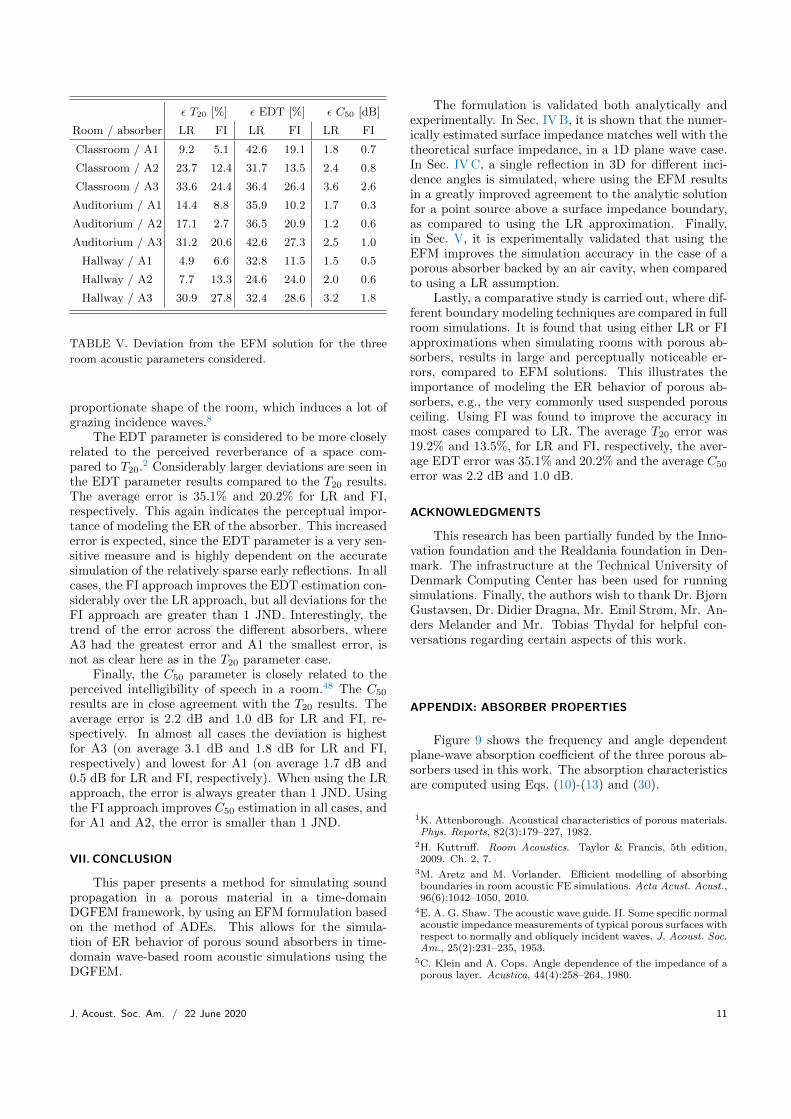
ε T20 [%] ε EDT [%] ε C50 [dB]
Room / absorber LR FI LR FI LR FI
Classroom / A1 9.2 5.1 42.6 19.1 1.8 0.7
Classroom / A2 23.7 12.4 31.7 13.5 2.4 0.8
Classroom / A3 33.6 24.4 36.4 26.4 3.6 2.6
Auditorium / A1 14.4 8.8 35.9 10.2 1.7 0.3
Auditorium / A2 17.1 2.7 36.5 20.9 1.2 0.6
Auditorium / A3 31.2 20.6 42.6 27.3 2.5 1.0
Hallway / A1 4.9 6.6 32.8 11.5 1.5 0.5
Hallway / A2 7.7 13.3 24.6 24.0 2.0 0.6
Hallway / A3 30.9 27.8 32.4 28.6 3.2 1.8
TABLE V. Deviation from the EFM solution for the three
room acoustic parameters considered.
proportionate shape of the room, which induces a lot ofgrazing incidence waves.8
The EDT parameter is considered to be more closelyrelated to the perceived reverberance of a space com-pared to T20.2 Considerably larger deviations are seen inthe EDT parameter results compared to the T20 results.The average error is 35.1% and 20.2% for LR and FI,respectively. This again indicates the perceptual impor-tance of modeling the ER of the absorber. This increasederror is expected, since the EDT parameter is a very sen-sitive measure and is highly dependent on the accuratesimulation of the relatively sparse early reflections. In allcases, the FI approach improves the EDT estimation con-siderably over the LR approach, but all deviations for theFI approach are greater than 1 JND. Interestingly, thetrend of the error across the different absorbers, whereA3 had the greatest error and A1 the smallest error, isnot as clear here as in the T20 parameter case.
Finally, the C50 parameter is closely related to theperceived intelligibility of speech in a room.48 The C50
results are in close agreement with the T20 results. Theaverage error is 2.2 dB and 1.0 dB for LR and FI, re-spectively. In almost all cases the deviation is highestfor A3 (on average 3.1 dB and 1.8 dB for LR and FI,respectively) and lowest for A1 (on average 1.7 dB and0.5 dB for LR and FI, respectively). When using the LRapproach, the error is always greater than 1 JND. Usingthe FI approach improves C50 estimation in all cases, andfor A1 and A2, the error is smaller than 1 JND.
VII. CONCLUSION
This paper presents a method for simulating soundpropagation in a porous material in a time-domainDGFEM framework, by using an EFM formulation basedon the method of ADEs. This allows for the simula-tion of ER behavior of porous sound absorbers in time-domain wave-based room acoustic simulations using theDGFEM.
The formulation is validated both analytically andexperimentally. In Sec. IV B, it is shown that the numer-ically estimated surface impedance matches well with thetheoretical surface impedance, in a 1D plane wave case.In Sec. IV C, a single reflection in 3D for different inci-dence angles is simulated, where using the EFM resultsin a greatly improved agreement to the analytic solutionfor a point source above a surface impedance boundary,as compared to using the LR approximation. Finally,in Sec. V, it is experimentally validated that using theEFM improves the simulation accuracy in the case of aporous absorber backed by an air cavity, when comparedto using a LR assumption.
Lastly, a comparative study is carried out, where dif-ferent boundary modeling techniques are compared in fullroom simulations. It is found that using either LR or FIapproximations when simulating rooms with porous ab-sorbers, results in large and perceptually noticeable er-rors, compared to EFM solutions. This illustrates theimportance of modeling the ER behavior of porous ab-sorbers, e.g., the very commonly used suspended porousceiling. Using FI was found to improve the accuracy inmost cases compared to LR. The average T20 error was19.2% and 13.5%, for LR and FI, respectively, the aver-age EDT error was 35.1% and 20.2% and the average C50
error was 2.2 dB and 1.0 dB.
ACKNOWLEDGMENTS
This research has been partially funded by the Inno-vation foundation and the Realdania foundation in Den-mark. The infrastructure at the Technical University ofDenmark Computing Center has been used for runningsimulations. Finally, the authors wish to thank Dr. BjørnGustavsen, Dr. Didier Dragna, Mr. Emil Strøm, Mr. An-ders Melander and Mr. Tobias Thydal for helpful con-versations regarding certain aspects of this work.
APPENDIX: ABSORBER PROPERTIES
Figure 9 shows the frequency and angle dependentplane-wave absorption coefficient of the three porous ab-sorbers used in this work. The absorption characteristicsare computed using Eqs. (10)-(13) and (30).
1K. Attenborough. Acoustical characteristics of porous materials.Phys. Reports, 82(3):179–227, 1982.
2H. Kuttruff. Room Acoustics. Taylor & Francis, 5th edition,2009. Ch. 2, 7.
3M. Aretz and M. Vorlander. Efficient modelling of absorbingboundaries in room acoustic FE simulations. Acta Acust. Acust.,96(6):1042–1050, 2010.
4E. A. G. Shaw. The acoustic wave guide. II. Some specific normalacoustic impedance measurements of typical porous surfaces withrespect to normally and obliquely incident waves. J. Acoust. Soc.Am., 25(2):231–235, 1953.
5C. Klein and A. Cops. Angle dependence of the impedance of aporous layer. Acustica, 44(4):258–264, 1980.
J. Acoust. Soc. Am. / 22 June 2020 11

a) A1 LR. b) A1 ER. c) A1 FI.
d) A2 LR. e) A2 ER. f) A2 FI.
g) A3 LR. h) A3 ER. i) A3 FI.
FIG. 9. (Color online) Frequency and angle dependent plane-wave absorption coefficient for the absorbers used.
6D. B. Bliss. and S. E. Burke. Experimental investigation ofthe bulk reaction boundary condition. J. Acoust. Soc. Am.,71(3):546–551, 1982.
7D.J. Sides and K.A. Mulholland. The variation of normal layerimpedance with angle of incidence. J. Sound Vib., 14(1):139–142,1971.
8M. Hodgson and A. Wareing. Comparisons of predicted steady-state levels in rooms with extended- and local-reaction boundingsurfaces. J. Sound Vib., 309(1):167–177, 2008.
9B. Yousefzadeh and M. Hodgson. Energy- and wave-based beam-tracing prediction of room-acoustical parameters using differentboundary conditions. J. Acoust. Soc. Am., 132(3):1450–1461,
2012.10K. Gunnarsdottir, C.-H. Jeong, and G. Marbjerg. Acoustic be-
havior of porous ceiling absorbers based on local and extendedreaction. J. Acoust. Soc. Am., 137(1):509–512, 2015.
11C.-H. Jeong. Guideline for adopting the local reaction assump-tion for porous absorbers in terms of random incidence absorp-tion coefficients. Acta Acust. Acust., 97(5):779–790, 2011.
12M. A. Biot. The theory of propagation of elastic waves in afluid-saturated porous solid. I. low frequency range. II. higherfrequency range. J. Acoust. Soc. Am., 28:168–191, 1956.
12 J. Acoust. Soc. Am. / 22 June 2020

13J. F. Allard and N. Atalla. Propagation of Sound in Porous Me-dia: Modelling sound absorbing materials. Wiley, West Sussex,United Kingdom, 3rd edition, 2009. Ch. 3,5.
14R. Panneton. Comments on the limp frame equivalent fluid modelfor porous media. J. Acoust. Soc. Am., 122(6):EL217–EL222,2007.
15D. Botteldooren. Finite-difference time-domain simulation oflow-frequency room acoustic problems. J. Acoust. Soc. Am.,98(6):3302–3308, 1995.
16A. Craggs. A finite element method for free vibration of airin ducts and rooms with absorbing walls. J. Sound Vib.,173(4):568–576, 1994.
17J. A. Hargreaves, L. R. Rendell, and Y. W. Lam. A framework forauralization of boundary element method simulations includingsource and receiver directivity. J.Acoust. Soc. Am., 145(4):2625–2637, 2019.
18S. Bilbao. Modeling of complex geometries and boundary condi-tions in finite difference/finite volume time domain room acous-tics simulation. IEEE Trans. Audio, Speech, Lang. Proc.,21(7):1524–1533, 2013.
19F. Pind, A. P. Engsig-Karup, C. H. Jeong, J. S. Hesthaven, M. S.Mejling, and J. Strømann Andersen. Time domain room acousticsimulations using the spectral element method. J. Acoust. Soc.Am., 145(6):3299–3310, 2019.
20H. Wang, I. Sihar, R. Pagan Munoz, and M. Hornikx. Roomacoustics modelling in the time-domain with the nodal discontin-uous Galerkin method. J. Acoust. Soc. Am., 145(4):2650–2663,2019.
21J. S. Hesthaven and T. Warburton. Nodal DiscontinuousGalerkin Methods—Algorithms, Analysis, and Applications.Springer, New York, 2008. Ch. 3.
22M. Vorlander. Computer simulations in room acoustics: Con-cepts and uncertainties. J. Acoust. Soc. Am., 133(3):1203–1213,2013.
23C. H. Jeong, G. Marbjerg, and J. Brunskog. Uncertainty of in-put data for room acoustic simulations. In Proc. Baltic-NordicAcoust. Meet., 2016.
24H. Wang and M. Hornikx. Time-domain impedance boundarycondition modeling with the discontinuous galerkin method forroom acoustics simulations. J. Acoust. Soc. Am., 147(4):2534–2546, 2020.
25S. Bilbao, B. Hamilton, J. Botts, and L. Savioja. Finite volumetime domain room acoustics simulation under general impedanceboundary conditions. IEEE Trans. Audio, Speech, Lang. Proc.,24(1):161–173, 2016.
26R. Tomiku, T. Otsuru, N. Okamoto, T. Okuzono, and T. Shibata.Finite element sound field analysis in a reverberation room usingensemble averaged surface normal impedance. In Proc. 40th Int.Cong. Expo. Noise Cont. Eng., 2011.
27D. Dragna, P. Pineau, and P. Blanc-Benon. A generalized recur-sive convolution method for time-domain propagation in porousmedia. J. Acoust. Soc. Am., 138(2):1030–1042, 2015.
28D. K. Wilson, V. E. Ostashev, and S. L. Collier. Time-domainequations for sound propagation in rigid-frame porous media. J.Acoust. Soc. Am., 116(4):1889–1892, 2004.
29J. Zhao, M. Bao, X. Wang, H. Lee, and S. Sakamoto. An equiv-alent fluid model based finite-difference time-domain algorithmfor sound propagation in porous material with rigid frame. J.Acoust. Soc. Am., 143(1):130–138, 2018.
30J. Zhao, Z. Chen, M. Bao, H. Lee, and S. Sakamoto. Two-dimensional finite-difference time-domain analysis of sound prop-agation in rigid-frame porous material based on equivalent fluidmodel. Appl. Acoust., 146:204–212, 2019.
31T. Okuzono, N. Shimizu, and K. Sakagami. Predicting absorp-tion characteristics of single-leaf permeable membrane absorbersusing finite element method in a time domain. Appl. Acoust.,151:172–182, 2019.
32Y. Miki. Acoustical properties of porous materials—modifications of Delany-Bazley models. J. Acoust. Soc. Jap.,
11(1):19–24, 1990.33D. Lafarge, P. Lemarinier, J. F. Allard, and V. Tarnow. Dynamic
compressibility of air in porous structures at audible frequencies.J. Acoust. Soc. Am., 102(4):1995–2006, 1997.
34B. Gustavsen and A. Semlyen. Rational approximation of fre-quency domain responses by vector fitting. IEEE Trans. Pow.Del., 14(3):1052–1061, 1999.
35B. Gustavsen. Fast passivity enforcement for pole-residue modelsby perturbation of residue matrix eigenvalues. IEEE Trans. Pow.Del., 23(4):2278–2285, 2008.
36C. Hopkins. Sound insulation. Butterworth-Heinemann, Oxford,United Kingdom, 1st edition, 2007. Ch. 4.
37J. S. Hesthaven and C. H. Teng. Stable spectral methods ontetrahedral elements. SIAM J. Sci. Comput., 21(6):2352–2380,2000.
38M.H. Carpenter and C. Kennedy. Fourth-order 2N-storageRunge-Kutta schemes. NASA report TM 109112, NASA Lan-gley Research Center, 1994.
39A.P. Engsig-Karup, C. Eskilsson, and D. Bigoni. A stabilisednodal spectral element method for fully nonlinear water waves.J. Comput. Phys., 318:1–21, 2016.
40S.-I. Thomasson. Reflection of waves from a point source by animpedance boundary. J. Acoust. Soc. Am., 59(4):780–785, 1976.
41U. Ingard. On the reflection of a spherical sound wave from aninfinite plane. J. Acoust. Soc. Am., 23(3):329–335, 1951.
42C. H. Jeong. Absorption and impedance boundary conditionsfor phased geometrical-acoustics methods. J. Acoust. Soc. Am.,132(4):2347–2358, 2012.
43ISO 354. Acoustics—Measurement of sound absorption in a re-verberation room. International organization for standardization,2003.
44M. Ren and F. Jacobsen. A method of measuring the dynamicflow resistance and reactance of porous materials. Appl. Acoust.,39(4):265–276, 1993.
45J. S. Suh and P. A. Nelson. Measurement of transient responseof rooms and comparison with geometrical acoustic models. J.Acoust. Soc. Am., 105(4):2304–2317, 1999.
46R. Kirby. On the modification of Delany and Bazley fomulae.Appl. Acoust., 86:47–49, 2014.
47ISO 3382-1. Acoustics—Measurement of room acousticparameters—Part 1: Performance spaces. International orga-nization for standardization, 2009.
48J.S. Bradley, R. Reich, and S.G. Norcross. A just noticeabledifference in C50 for speech. Appl. Acoust., 58(2):99–108, 1999.
J. Acoust. Soc. Am. / 22 June 2020 13

14 J. Acoust. Soc. Am. / 22 June 2020

PAPER P5
118

Massively Parallel Nodal DiscontinousGalerkin Finite Element MethodSimulator for Room Acoustics
Journal TitleXX(X):1–15c©The Author(s) 2016
Reprints and permission:sagepub.co.uk/journalsPermissions.navDOI: 10.1177/ToBeAssignedwww.sagepub.com/
SAGE
Anders Melander1, Emil Strøm1, Finnur Pind2,3, Allan P. Engsig-Karup1, Cheol-Ho Jeong3,Tim Warburton4, Noel Chalmers4 and Jan S. Hesthaven5
AbstractWe present a massively parallel and scalable nodal Discontinuous Galerkin Finite Element Method (DGFEM) solverfor the time-domain linearised acoustic wave equations. The solver is implemented using the libParanumal finiteelement framework with extensions to handle curvilinear geometries and frequency dependent boundary conditionsof relevance in practical room acoustics. The implementation is benchmarked on heterogeneous multi-device many-core computing architectures, and high performance and scalability are demonstrated for a problem that is consideredexpensive to solve in practical applications. In a benchmark study, scaling tests show that multi-GPU support givesthe ability to simulate large rooms, over a broad frequency range, with realistic boundary conditions, both in termsof computing time and memory requirements. Furthermore, numerical simulations on two non-trivial geometries arepresented, a star-shaped room with a dome and an auditorium. Overall, this shows the viability of using a multi-deviceaccelerated DGFEM solver to enable realistic large-scale wave-based room acoustics simulations using massivelyparallel computing.
KeywordsHigh-Performance Computing, Multi-Device Acceleration, Heterogeneous CPU-GPU Computing, Room AcousticSimulation, Discontinuous Galerkin Method.
1. Introduction
Room acoustic simulations are widely used in, e.g., buildingdesign, virtual reality and hearing research. The task ischallenging from a computational point of view as itinvolves simulating large and complex domains, over abroad frequency spectrum and long times. Room sizes rangefrom 30 m3 to 30,000 m3, our auditory system can hearfrequencies from 20 Hz to 20 kHz, and sound typicallylasts in rooms somewhere between 0.5 s (living room) to3.0 s (concert hall). Historically, the prevailing approachhas been to apply geometrical acoustics methods (1), suchas the image source method (2) or ray-tracing (3), wherethe acoustic wave is approximated as a bundle of rays thatare propagated in the room using the laws of ray optics.This reduces the computational task considerably, but theapproximation is only appropriate in the high-frequencylimit. At low-mid frequencies, wave phenomena such asdiffraction and interference dominate and other simulationmethods must be used.
This motivates the use of wave-based methods, where thegoverning partial differential equations that describe wavemotion are solved numerically. Given the right input data,these methods are very accurate, since no approximationto the wave propagation is made and all wave phenomenaare inherently accounted for. Several different numericaltechniques have been applied, such as the finite-differencetime-domain (FDTD) method (4), the pseudospectral time-domain (PSTD) method (5), the finite volume method (FVM)(6), the boundary element method (BEM) (7), and the
finite element method (FEM) (8). Recently, nodal high-order-accurate variants of the FEM, such as the spectralelement method (SEM) (9) and the discontinuous Galerkinfinite element method (DGFEM) (10), have been appliedto simulate room acoustics. High-order methods result inbetter accuracy-per-computational-cost and they have thepotential to significantly reduce the runtime of simulations,and are a must for having good accuracy in wave propagationproblems over long integration times (11). The nodalDGFEM is particularly well suited for room acousticsimulations, because it combines the attractive featuresof geometric flexibility, high-order accuracy, suitabilityfor parallel computing, and lean memory usage. In theDGFEM schemes, the solution is computed locally for eachelement, with communication between elements only at theelement boundaries. This data locality can be utilized forparallelization of the solver.
1Scientific Computing Section, Department of Applied Mathematicsand Computer Science, Technical University of Denmark, Kgs. Lyngby,Denmark.2Henning Larsen, Copenhagen, Denmark.3Acoustic Technology Group, Department of Electrical Engineering,Technical University of Denmark, Kgs. Lyngby, Denmark.4Department of Mathematics, Virgina Tech, United States.5Chair of Computational Mathematics and Simulation Science, EcolePolytechnique Federale de Lausanne, Lausanne, Switzerland.
Corresponding author:Anders MelanderEmail: [email protected]
Prepared using sagej.cls [Version: 2017/01/17 v1.20]

2 Journal Title XX(X)
The major drawback of wave-based methods is theassociated high computational cost. Simulating large spaces(larger than, say, 1,000 m3) into the mid frequency range (upto and beyond 1 kHz) typically requires tens or hundredsof millions of degrees of freedom (DoF). Despite progressin numerical methodology, wave-based methods are mostlyapplied to small rooms at very low frequencies. However,with the rapid advancements in many-core computinghardware, massively parallel high-performance computing(HPC) – in particular, the use of graphics processingunits (GPUs) for scientific computing – offers a way togreatly extend the usability of wave-based methods tolarge spaces and for a broad spectrum of frequencies.There is some past work on the HPC implementation ofwave-based room acoustic simulations. Lopez et al. (12)and Spa et al. (13) studied the GPU implementation ofthe FDTD method and found that, when implementedefficiently, the use of GPUs could drastically improve thecomputational performance. The FDTD method, like theDGFEM, lends itself naturally to parallelization but has alow arithmetic complexity. Takahashi et al. (14) studied theGPU acceleration of the BEM when applied to the frequencydomain Helmholtz equation and reported a considerableimprovement in performance. Lastly, Morales et al. (15)considered a distributed memory multi-CPU implementationof an adaptive rectangular decomposition (ARD) algorithmfor room acoustic simulations and found that they couldsimulate large domains over broad frequency ranges usingthe HPC setup. While the ARD implementation of Moraleset al. is described as efficient, it cannot handle complexgeometries or non-trivial boundary conditions (BCs).
The goal of this work is to introduce the details of aHPC approach to simulate three-dimensional room acousticsusing the DGFEM. To the best of our knowledge, this isthe first time a massively parallel GPU-accelerated wave-based DGFEM room acoustic simulator is presented inthe literature. The simulator is written in C/C++ withMessage Passing Interface (MPI) as its backbone, andthe device-interfacing is implemented using the singlekernel language for parallel programming Open ConcurrentCompute Abstraction (OCCA) (16) for portable multi-threading code development across different many-corehardware architectures. Curvilinear meshes and locallyreacting frequency independent and frequency dependentimpedance boundary conditions are supported in theimplementation.
The paper is organized as follows. Section 2 presents thegoverning equations and the boundary conditions. Section3 presents the numerical discretization of the governingequations. In Section 4, the HPC implementation is describedand Section 5 contains several numerical experiments thatoffer insights into the performance of the simulator. Finally,some concluding remarks are offered in Section 6.
2. The mathematical model
Acoustic wave propagation in a lossless medium is governedby the coupled first order system of partial differential
equations
vt = −1
ρ∇p,
pt = −ρc2∇ · v,(1)
where v(x, t) [m/s] is the particle velocity at position x inthe domain Ω at time t, p(x, t) is the acoustic pressure [Pa],ρ is the density of air and c is the speed of sound in air. Inthis work, we use ρ = 1.2kg/m3 and c = 343 m/s. We letu, v and w be the Cartesian coordinates x, y, z parts of thevelocity field v = [u, v, w]T .
2.1 Boundary conditionsTo solve realistic problems, boundary conditions are needed,to accurately capture the absorption properties of theboundary of the domain ∂Ω. In the following, we willintroduce the boundary condition types that have beenimplemented in the DGFEM solver. These are rigid,frequency independent and frequency dependent boundaryconditions.
2. 1. 1. RigidThe rigid boundary condition perfectly reflects the impingingwave back into the domain Ω. Mathematically this isexpressed as
n · v = 0 on ∂Ω, (2)
where n is the outward pointing normal of the boundarysurface ∂Ω.
2. 1. 2. Locally-reacting frequency independentThe frequency independent impedance boundary conditionadds absorption to the domain boundaries, with allfrequencies being absorbed equally. The absorption isdictated by the normal incidence surface impedance Z. Thenormal velocity at the boundary becomes
n · v = vn =p
Z= pY, (3)
where Y is the normal boundary admittance. Using highvalues of Z implies a highly reflective boundary conditions,whereas values close to the characteristic impedance of theair Zair = ρc results in a highly absorptive boundary.
2. 1. 3. Locally-reacting frequency dependentMost real world surfaces exhibit frequency dependentabsorption. Mathematically, this can be written as
vn =p(ω)
Z(ω)= p(ω)Y (ω), (4)
where ω is the angular frequency and (vn, p) denotethe Fourier transformed normal velocity and pressure,respectively. Z(ω) is no longer constant, as in the frequencyindependent case, but is a complex function of the angularfrequency. For a particular surface, Z(ω) can be measured,e.g., in an impedance tube or using pressure-velocitysensors. Alternatively, several material models exist toestimate surface impedance of many common materials andconstructions.
Prepared using sagej.cls

Melander et al. 3
To incorporate the frequency dependent boundaryconditions accurately and efficiently into the time-domainsimulation, the method of auxiliary differential equations(ADEs) can be used (9; 17). In the ADE method, the surfaceadmittance is approximated as a rational function, defined as,
Y (ω) =a0 + ...+ aN (−jω)N
1 + ...+ bN (−jω)N, (5)
which can be rewritten using a partial fraction decomposition
Y (ω) =Y∞ +
Q∑
k=1
Akλk − jω
+
S∑
k=1
(Bk + jCk
αk + jβk − jω+
Bk − jCkαk − jβk − jω
).
(6)
Here Q is the number of real poles, S is the number ofcomplex conjugate pole pairs of Y (ω), λk are the real poles,αk ± jβk are the complex conjugate pole pairs, and Y∞,Ak, Bk and Ck are numerical coefficients. For causality, λkand αk must be semi-positive. Furthermore, for each set ofnumerical coefficients, the passivity of the multipole modelmust be checked. If the model is non-passive, it will addenergy to the simulation, potentially leading to a blowupof the solution. The total number of poles Npoles = Q+ 2S,should be chosen large enough to satisfy an error thresholdof the multipole approximation of the boundary admittance.
By applying the inverse-Fourier transform to (4), we get
vn(t) =
∫ t
−∞p(t′)y(t− t′)dt′. (7)
Then by applying the inverse Fourier transform to (6) andinserting the result into (7), the expression for the velocityvn at the boundary becomes
vn(t) =Y∞p(t) +
Q∑
k=1
Akφk(t)+
S∑
k=1
2(Bkψ
(1)k (t) + Ckψ
(2)k (t)
),
(8)
where φk is the accumulator for the k’th real poles, andψ
(1)k and ψ
(2)k are the accumulators for the k’th complex
conjugate poles pairs. These accumulators are defined by aset of ordinary differential equations (ODEs)
dφkdt
λkφk = p(t),
dψ(1)k
dtαkψ
(1)k + βkψ
(2)k = p(t),
dψ(2)k
dtαkψ
(2)k − βkψ
(1)k = 0.
(9)
Thus, when using the ADE method, an additional set ofODEs must be solved at the boundary in each time step.The added computational cost due to this additional setof ODEs is relatively low, as the amount of extra ODEsneeded to solve is small compared to the system that mustbe solved for the acoustic wave equations. In total, therewill be Npoles times the number of boundary nodes with
frequency dependent boundary condition ODEs to solve.This extra work generally grows significantly slower than thetotal number of nodes in a domain when the mesh resolutionincreases in the domain.
3. The numerical model
3.1 Spatial discretizationThe spatial derivatives in (1) are discretized using DGFEM.DGFEM is a high-order method (18) capable of solving thetime-domain acoustic partial differential equations within adomain Ω, subject to an appropriate set of boundary andinitial conditions. The spatial domain is tessellated by Knon-overlapping elements as
Ω ' Ωh =K⋃
k=1
Dk. (10)
In this work, the elements are taken to be tetrahedralelements in the three-dimensional space. On each of theseelements the solution variables v and p are expressed onthe k’th element in terms of polynomial basis functions andcorresponding modal or nodal coefficients. This is expressedas
vkh(x, t) =
Np∑
n=1
vkn(t)φn(x) =
Np∑
n=1
vkh(xkn, t)`kn(x),
pkh(x, t) =
Np∑
n=1
pkn(t)φn(x) =
Np∑
n=1
pkh(xkn, t)`kn(x).
(11)
Here φn(x) is the hierarchical modal basis function and`ki (x) is the corresponding nodal Lagrange polynomial basisfunction on element Dk. vkn(t) and pkn(t) are the modalcoefficients for the modal basis functions, and vkh(xkn, t)and pkh(xkn, t) are the corresponding nodal coefficientsfor the nodal basis functions. The modal basis functionsare assumed to be orthonormal as this simplifies severalneeded computations. On each element xkn is a nodedistribution of Np = ((N + 1)(N + 2)(N + 3))/6 distinctnodal interpolation points, where N is the order of the basisfunctions. An α-optimized nodal distribution is used dueto its low Lebesque constants (19). The solutions on theelements are used to approximate the global solutions v andp in terms of direct sums
v ≈ vh =K⊕
k=1
vkh, p ≈ ph =K⊕
k=1
pkh. (12)
The strong formulation of the governing equations, whenusing the nodal basis series to represent the unknownvariables vkh and pkh, takes the following form∫
Dk
∂vkh∂t
`kn(x)dx =− 1
ρ
∫
Dk
∇pkh`kn(x)dx
+1
ρ
∫
∂Dk
n(pkh − p∗
)`kn(x)dx,
∫
Dk
∂pkh∂t
`kn(x)dx =−∫
Dk
ρc2∇ · vkh`kn(x)dx
+ ρc2∫
∂Dk
n ·(vkh − v∗
)`kn(x)dx.
(13)
Prepared using sagej.cls

4 Journal Title XX(X)
where the star-labeled terms denote numerical fluxes thatpropagate the solution between elements. This can berewritten in a discrete formulation using matrix-basedoperators for integration and differentiation
dukhdt
= −1
ρDkxpkh +
1
ρLk(pkh − p∗
)nx, (14a)
dvkhdt
= −1
ρDkypkh +
1
ρLk(pkh − p∗
)ny, (14b)
dwkhdt
= −1
ρDkzpkh +
1
ρLk(pkh − p∗
)nz, (14c)
dpk
dt= −ρc2
(Dxukh +Dyvkh +Dzwkh
)
+ ρc2Lkn ·(vkh − v∗
). (14d)
The matrix operations on the right hand side are expressedin terms of the operators defined on the reference elements
Dr = VrV−1, Ds = VsV−1, Dt = VtV−1,
M = (VVT )−1.(15)
Here Vij ≡ φj(ri) is the generalized Vandermonde matrixand (VX)ij ≡ ∂φj(ri)/∂X are defined in terms of referenceelement coordinates X = r, s, t.
These operators can, via the chain rule of the continuousvariables, e.g.,
∂f(x)
∂x=∂r
∂x
∂f(x)
∂r+∂s
∂x
∂f(x)
∂s+∂t
∂x
∂f(x)
∂t, (16)
be related to the corresponding discrete differentialoperations in the physical domain for each element
Dkx = rkxDr + skxDs + tkxDt,Dky = rkyDr + skyDs + tkyDt,Dkz = rkzDr + skzDs + tkzDt.
(17)
Furthermore, we introduce the lift operator L needed for theincorporation of boundary conditions via numerical fluxes atthe element edges
L = (M)−1 E , M = (VVT )−1, (18)
where E is the column-wise concatenation of the face massmatrices.
To avoid computing and storing these matrices for everyelement, the matrix operators are determined for a referenceelement, and a geometric mapping from the arbitrary meshelements to the reference elements is used, e.g.,
Mk = Jk(VVT )−1, (19)
where Jk is the Jacobian of the local map of the k’th elementto the reference element.
The choice of the numerical flux stabilizes the dispersionand dissipation properties of the DGFEM scheme. In thiswork, the upwind flux is chosen. The upwind flux combineslow dispersion errors over a wide range of frequencies withdissipation for underresolved frequencies (20; 21). To derivethe upwinding flux, a Riemann problem at each element edgemust be solved. We start by rewriting (1) in the quasi-linear
form of a hyperbolic system
∂q
∂t+∇ · F(q) =
∂q
∂t+ Aj
∂q
∂xj= 0 (20)
where q(x, t) = [u, v, w, p]T is the acoustic variable vector,j ∈ [x, y, z] is the Cartesian coordinate index and Aj is aconstant flux Jacobian matrix, given as
Aj =
0 0 0δxj
ρ
0 0 0δyj
ρ
0 0 0δzjρ
ρc2δxj ρc2δyj ρc2δzj 0
, (21)
where δij denotes the Kronecker delta function. The flux ofthe system is defined as
F = [Axq,Ayq,Azq]. (22)
We are interested in the numerical flux along the outwardpointing element boundary normal n, which leads to thecreation of the following operator
N = n · F = nxAx + nyAy + nzAz. (23)
Applying an eigendecomposition on N yields
N = RDR−1, (24)
where
R =
nx
ρc − nx
ρc − nz
nx− ny
nxny
ρc − ny
ρc 0 1nz
ρc − nz
ρc 1 0
1 1 0 0
,
D =
c 0 0 00 −c 0 00 0 0 00 0 0 0
.
(25)
Here the diagonal of D contains the eigenvalues of N.Since all eigenvalues are real, the system is hyperbolic, andtherefore the eigenvalues represent the speeds of propagationof information of the characteristic variables b, defined asR−1q = b (22).
By splitting the eigenvalue matrix D into its positive andnegative parts
D = D+ + D−
=
c 0 0 00 0 0 00 0 0 00 0 0 0
+
0 0 0 00 −c 0 00 0 0 00 0 0 0
,
(26)
D+ corresponds to the parts of b where the direction isalong the normal vector n, meaning the information isleaving the element, whereas D− corresponds to the partsof b where the direction is opposite n, implying that theinformation is entering the element. In the numerical flux weseek to combine the information from the current elementboundary point, given in q−h with the information from theneighbouring element boundary point, given in q+
h . Since
Prepared using sagej.cls

Melander et al. 5
n · F = Nqh, the following holds
n · F = RDR−1qh = RD+R−1qh + RD−R−1qh.
(27)
By the properties of D+ and D−, this results in thenumerical upwind flux
(n · F)∗ = RD+R−1q−h + RD−R−1q+h . (28)
Boundary conditions are weakly enforced through thenumerical flux terms. For element faces that lie on thedomain boundary, q+
h needs to be defined according tothe boundary conditions. For surface impedance boundaryconditions, an averaging approach is used to imposeDirichlet conditions, where the neighboring value is given byp+h = p−h and v+
h = −v−h + 2gv , where n · gv = vn, withvn given by either (3) or (8). Thus, at the domain boundarynodes, the flux term in (14d) becomes n · (vkh − v∗) = n ·v−h − vn.
3. 2. Temporal discretization and stabilityThe semi-discrete system in (14) can be expressed as ageneral form ODE
dqhdt
= L(qh(t), t), (29)
where L is the spatial operator. This ODE system isintegrated in time using a low-storage 4th order explicitRunge-Kutta time-stepping method,
q(0)h = qnh,
i ∈ [1, . . . , 5] :
k(i) = aik
(i−1) + ∆tL(q(i−1)h , tn + ci∆t),
q(i)h = q
(i−1)h + bik
(i),
qn+1h = q
(5)h ,
(30)
where ∆t = tn+1 − tn is the time step size and thecoefficients ai, bi, ci are given in Ref. (23).
Explicit time-stepping methods impose a conditionalstability criterion, ∆t ≤ C1/(max |λe|), where λe are theeigenvalues of the spatial discretization and C1 is a constantrelated to the size of the stability region of the time-steppingmethod (9). There are two mechanisms at play that influencethe maximum allowed time step: 1) the eigenvalue spectrumsof the matrix operators, and 2) the stiffness of the ADEs. InDGFEM, the matrix operator eigenvalue spectrum scales asmax |λe| ∼ C2cN
2γ , where the C2 constant is dictated bythe size of the smallest mesh element and γ is the highestorder of differentiation in the governing equations (γ = 1,here) (24). Thus, in this work, the time step size is given as
∆t = CCFL min(∆xl)1
c
1
N2, (31)
where ∆xl is the smallest edge length of the mesh elementsand CCFL is a constant of O(1).
No measures have been taken to automatically addressthe potential stiffness of the ADEs. Implicit-explicit time-stepping (25) or stiffness restriction, by means of aconstrained multipole mapping process (26), could be used
to ensure the ADEs do not cause a numerical instability.However, in all numerical experiments, the spatial schemeis found to determine the condition on the stable time stepsize.
3. 3. Meshing and curvilinear geometryMeshing is done using the open-source meshing tool gmsh(27). When affine (straight-sided) elements are used, themesh generator is used to generate a low-order finite elementmesh, and the simulator then adds the α-optimized nodes todefine the high-order mesh elements, in accordance with thepolynomial basis order used.
When using high-order basis functions, the mesh elementscan be made bigger without sacrificing accuracy, which isattractive from a cost-efficiency point of view, but might limitthe ability to handle complex geometries. Using curvilinearelements, where the internal high-order mesh nodes areshifted to better fit the geometry, is a way to mitigate this(9). For room acoustic simulations, this is a particularlyimportant feature, since most real-world rooms containcurved or complex shaped boundary surfaces.
Currently, gmsh has the ability to generate a high-order curvilinear mesh, however, only with equidistant nodedistributions. This is sub-optimal, because of the rapidgrowth of the Lebesque constant associated with equidistantnode distributions (28). Our solution here is to apply aninterpolation post-processing step on the high-order meshgenerated by gmsh, where the equidistant nodes are movedto the α-optimized curvilinear node positions. This can bedone by re-interpolating the node position by representingthe coordinates as polynomial series, cf. (11). Then, let r andre be the r, s and t coordinates in the reference element forα-optimized and equidistant node distributions, respectively.Using a hierarchical modal basis, the coefficients r of thisrepresentation can be determined from
r = V r, re = Vre r, (32)
where (Vre)ij ≡ φj(rei ), using same basis used to define Vbut defined in terms of the different set of equidistant nodes.This implies the relationship between the node distributions
r = V(Vre)−1re (33)
from which an interpolation matrix I : re 7→ r is defined as
I = V(Vre)−1. (34)
Using this operator offers a way to go from thegmsh generated curvilinear mesh with equidistant nodedistribution to a curvilinear mesh with α-optimized nodedistribution.
4. HPC implementationThe proposed HPC room acoustics simulator is based on theopen source libParanumal framework (29; 30), whichis a set of highly optimized finite element flow solversfor heterogeneous (GPU/CPU) systems. A Message PassingInterface (MPI) is used to handle communication betweenCPUs. Note, that when we use the term ‘CPU’, it refers toone single CPU core, while ‘GPU’ refers to the entire GPU.
Prepared using sagej.cls

6 Journal Title XX(X)
MPI works by treating each CPU core as its own entity,with its own separate memory. Information can be sharedbetween CPU cores through the messaging interface. Inpractice this means that libParanumal splits the domaininto different chunks. This is illustrated in Fig. 1. Each CPUcore only stores the simulation information needed for thecomputations in elements belonging to its own part of thedomain. However, as Fig. 1 illustrates, the CPUs share aninterface between them, where information has to be sharedfor the acoustic wave to propagate from one CPU to thenext. This means that for some elements, the numericalflux has to be computed based on neighbouring elementsthat are located on a different CPU, requiring that MPIcommunication between cores must take place. This is calleda halo exchange. The same communication is used whenGPUs are used.
Figure 1. Example of a three CPU core setup. The domain issplit into three chunks that are stored in separate CPU coresmemory.
When executing the code on GPUs, the code is structuredsuch that each CPU core is assumed to have access to oneGPU, e.g., only CPU0 can communicate directly with GPU0.This implies that the interface communications betweenCPU cores become more costly, as compared to only usingCPUs, because CPU0 must copy all interface informationfrom GPU0 into RAM on CPU0, before it can communicatethis information to CPUx through MPI, where 0 < x ≤M − 1 denotes an arbitrary CPU core out of the totalof M CPUs. CPUx has to copy the received interfaceinformation to its connected GPU, GPUx. In other words,using GPUs introduces an additional communication step,and therefore additional communication overhead, betweenCPU and GPU in each time-stepping stage. This implies thatwe expect worse scaling of computational performance whenadding additional CPU-GPU pairs to run the simulation, ascompared to only using CPUs. However, using the GPUsis very attractive because of the very large number ofcores available and high on-chip bandwidth, so much fastersimulation is expected when using GPUs compared to CPUs.The communication structure can be seen in Figure 2, wherethe red arrows are the CPU and GPU communications andthe blue arrows are the MPI communications.
Figure 2. Communication overview of M total heterogeneousCPU-GPU pairs. All CPUs can communicate through MPI,GPUs can only communicate through their attached CPU byproxy.
The implementation of one stage of the time-steppingmethod in (30), including all the interface communication,is summarized in Algorithm 1. The GPU functions, calledkernels, must be launched in every iteration of the timestepping algorithm.
Algorithm 1: One stage of the LSERK time-steppingmethod
Input: Previous stage q(i−1)h
Result: An updated stage q(i)h
1 GPU to CPU memory copy of interface nodes(CPU/GPU). Simultaneously initiate volume integralcompute kernel (GPU).
2 Initiate interface MPI communication (CPU).3 CPU to GPU memory copy of interface nodes
(CPU/GPU).4 Initiate surface integral compute kernel (GPU).5 Update based on current stage (GPU).
On most modern graphics cards the memory movementto/from pinned host memory and device memory can bedone with an on-board direct memory access (DMA) enginewhich can fully overlap with compute activity on the GPUdie. This means that the device-host communication and thevolume integral computation of the right hand side of (14)can start simultaneously, as shown in step 1. Ideally, thecommunication work in steps 1,2 and 3 is finished beforethe volume kernel finishes. This way, communication costsare completely hidden. This is possible because the volumekernel is completely asynchronous with respect to the host.Step 4, however, cannot start until all communication of steps1-3 is finished, and the volume kernel is finished.
As can be seen from the algorithm, the CPU-GPUpairs have to be synchronized in each stage, meaningthat an uneven workload distribution will cause poorperformance. For this reason, it is desirable to have theoverall communication work of each CPU equally balanced,as other CPU-GPU pairs will be locked in step 3 until theyhave sent/received all of the information needed. Overall,the amount of communication required in each time-step isconsiderable for high resolution simulations, which means
Prepared using sagej.cls

Melander et al. 7
that it cannot be expected that the simulator demonstratesperfect scaling on multiple GPUs.
5. Numerical experiments
All numerical experiments are carried out using the HPCsystem at the Technical University of Denmark (DTU)Computing Center. Three computing nodes are used, whereeach node consists of:
• CPU : 2 × Intel Xeon Gold 6142 @ 2.60 GHz,• GPU : 4 × NVIDIA Tesla V100 SXM2 32 GB,
with the three nodes being connected by InfiniBand. Thecompilers used for compilation are:
• GCC v7.4.0,• OpenMPI v3.1.3,• OCCA v1.0,• CUDA compilation tools v10.0.130.
For the scalability tests, we will use the setups of 1, 2, 4, 8,and 12 GPUs. Note that when running tests with 4 or lessGPUs, they will all be on the same node. This means thatwhen going from 4 to 8 GPUs there will be an additionalcost of transfer, as internal communication is not as fast as amemory copy within a node.
All simulations are performed using double-precisionfloating point numbers. If the numerical accuracy of thedouble is not required, one can change the datatype to floats.This change will result in a roughly 2× speed increase, anda decrease in the memory footprint by about the same factor.
5.1. Convergence
5.1.1. Cube domainAs an initial validation of the simulator, a convergence testin a cube domain with (x, y, z) ∈ [0, 1] and rigid boundariesis carried out. The simulation is initiated using a Gaussianpulse pressure initial condition
p(x, 0) = exp
(− (x− xs)2 + (y − ys)2 + (z − zs)2
sxyz
)
(35)where (xs, ys, zs) is the source position and sxyz = 0.3m2 is the spatial variance, which governs the frequencycontent of the pulse. For this case, an analytic solution exists(31). The domain is meshed using structured meshes oftetrahedral elements. We study both p-convergence, i.e., theerror behavior as a function of the basis function order fora fixed mesh, and h-convergence, i.e., the error behavior asa function of the mesh element size. The numerical erroris defined as e = ||pDGFEM − pTS||∞, where pDGFEM is thesimulated pressure in the entire field at t = 0.01s and pTS
is the true solution. The time step size is computed using alarge time step (close to the stability threshold), by havingCCFL = 1 in (31).
Figure 3 shows the resulting p-convergence, tested forthree different meshes, having varying resolution. Thefigure reveals the expected spectral convergence, i.e., anexponentially fast decay of errors, is indeed observed.
Figure 3. p-convergence for the rigid cube test case.
Figure 4 shows the h-convergence for different orders ofthe basis. Table 1 lists the resulting convergence rates. Thetable also includes convergence rates for a case where thetime step size has been reduced significantly (CCFL = 0.02).A convergence rate in the range O(hN ) and O(hN+1) isexpected (18). The results are mostly in good agreement withthe expected rates, with the exception of N = 1 and N = 2.This is explained by the meshes not being fine enough forthese low orders to give an accurate representation of theirconvergence. Furthermore, it is seen that reducing the timestep size has only marginal influence on the convergencerates, indicating that in this test case, the spatial errorsdominate.
Figure 4. h-convergence for the rigid cube test case.
N CCFL = 1 CCFL = 0.021 -0.778 -0.7782 -3.239 -3.2403 -3.919 -3.9204 -4.618 -4.6205 -5.752 -5.7526 -6.188 -6.1887 -7.754 -7.7478 -8.161 -8.166
Table 1. Convergence rates for the h-convergence study..
5.1.2. Cylinder domainConsider now a cylinder shaped domain, of 1 m height and 1m radius and having rigid boundaries. A convergence testis carried out, where the domain is meshed either usingaffine mesh elements or curvilinear mesh elements. Thereference solution here is computed using an extremely finemesh of affine elements (410, 308 elements) and N = 8basis function order. The numerical error is then defined as
Prepared using sagej.cls

8 Journal Title XX(X)
e = ||pDGFEM − pDGFEMfine || , where pDGFEM is the simulated
solution in 10 randomly chosen receiver points at t = 0.01and pDGFEM
fine is the simulated solution in the same receiverpoints for the fine mesh reference simulation.
Figure 5 shows the resulting p-convergence, tested forthree different meshes of varying resolution, using eitheraffine elements or curvilinear elements. When using affineelements, the high-order convergence is destroyed, as theconvergence rate flattens out for orders higher than N ≈3. However, when using the curvilinear elements, spectralconvergence is observed.
(a) Affine elements.
(b) Curvilinear elements.
Figure 5. p-convergence for the cylinder geometry using eitheraffine or curvilinear meshes.
Further insights are offered in Figure 6, where h-convergence is shown for both the affine and the curvilinearcase. It is seen that for the affine elements, a convergence rateof around O(h2) is achieved consistent with the geometricapproximation, whereas a much higher convergence rate isobserved for the curvilinear elements. However, the errorplateaus at around 10−7, which is likely due to aliasing errorsthat stem from the transformation Jacobians and normals nolonger being constant. This results in inexact integration ofvariable terms in the inner products used to compute thematrix based operators. Anti-aliasing techniques could beemployed to reduce the error further (32; 33). However,in practical room acoustics simulations, error levels below10−7 are rarely needed and, furthermore, such anti-aliasingtechniques increases the computational cost of the scheme.
5.2. Boundary condition validationA validation study of the locally reacting frequencydependent boundary conditions is carried out, using a normalincidence single reflection case. For this case, an analyticsolution exists (34). A 6 m × 10 m × 10 m rectangulardomain is meshed with an unstructured mesh of tetrahedral
(a) Affine elements.
(b) Curvilinear elements.
Figure 6. h convergence for the cylinder geometry using eitheraffine or curvilinear meshes.
elements. The frequency dependent impedance boundaryis the Y Z plane at x = 0. The resolution of the mesh isroughly 8 points per wavelength (PPW) at 1 kHz, the highestfrequency of interest. The source is placed 2 m from theimpedance boundary (S : (2, 5, 5) m) and the receiver isplaced between the source and the boundary (R : (1, 5, 5)m). The simulation duration is tfinal = 0.02 s, which ensuresthat no parasitic reflections from the other room surfacesarrive at the receiver position. A Gaussian pulse initialcondition, centered at the source position, with sxyz = 0.2m2 is used.
Two boundary conditions are considered; a porousmaterial mounted on a rigid backing (BC1) and a thinporous layer backed by an air cavity (BC2). The surfaceadmittance of the BCs are estimated using Miki’s model anda transfer matrix method (35; 36). Vector fitting is used forthe multipole mapping (37). The material is mapped in thefrequency range of 50 to 1500 Hz. An estimate of the relativemapping error is given by
ε =|Y (f)− Yfit(f)|
Y (f), (36)
where Y indicates the mean across frequency. Table 2summarizes the properties of the considered boundaryconditions and the multipole mapping. Note that more polesare needed in the mapping of BC1, because the admittanceresponse fluctuates more with frequency for this absorber.
Prepared using sagej.cls

Melander et al. 9
ID dmat d0 σmat Npoles εRe εIm
BC1 0.02 0.2 50, 000 8 0.0216 0.0177BC2 0.05 0.0 10, 000 4 0.0213 0.0071
Table 2. Material properties and multipole mapping error for theBCs used in the boundary validation study. dmat [m] is theporous material thickness, d0 [m] is the air cavity depth, σmat
[Ns/m4] is the flow resistivity of the porous material, Npoles is thenumber of poles used in the multipole mapping and εRe [%] andεIm [%] are the relative mapping errors of the real and imaginaryparts of the surface admittance, respectively.
.
Figure 7 shows the resulting Fourier transformed pressureresponses of the single reflection study. An excellent matchbetween the analytic solution and the simulation is found forboth BCs considered, both in terms of magnitude and phase.This confirms the high precision of the BC implementation.
(a) Magnitude.
(b) Phase.
Figure 7. Simulation of a single reflection from a locallyreacting frequency dependent impedance boundary comparedagainst the analytic solution.
5.4 Multi-GPU performance
5. 4. 1. Strong scaling
Strong scaling is characterised by how the runtime changeswhile keeping the problem size constant and increasingthe number of processing units. Thus the overall workloadis constant, while the workload of each processing unitdecreases, as the workload is split among an increasingnumber of processing units.
Four meshes of varying resolutions are constructed,described in Table 3. These meshes are used to analyse thestrong scaling of the simulator for two different polynomialorders, N = 4 and N = 6. In all cases, rigid BCs are used.
# of elements DoF N = 4 DoF N = 6Mesh 1 57k 1, 995k 4, 788kMesh 2 1, 266k 44, 310k 106, 344kMesh 3 3, 558k 124, 530k 298, 872kMesh 4 6, 583k 230, 405k 552, 972k
Table 3. Meshes and resulting DoF used for strong scalinganalysis, where k denotes kilo, i.e. ×1000.
A measure of the overall strong scaling computationalefficiency of the simulator is defined as
ηS =T bRM
b
TRM, (37)
where T bR denotes the runtime of a baseline case,M b denotesthe number of GPUs used for the baseline case, and TRand M denote the same for the comparison case. Thus ifηS = 1, perfect scaling occurs when going from M b to M .In practice, perfect scaling is impossible, as there is alwayssome latency introduced when scaling up the number ofprocessors used.
An array of simulations is carried out, using the meshesdefined in Table 3, and the runtime is recorded. The resultingstrong scaling computational efficiency is shown in Table 4.
#GPUs Mesh 1 Mesh 2 Mesh 3 Mesh 41 1 1 − −2 0.630 0.903 1 14 0.393 0.656 0.851 0.9138 0.290 0.586 0.704 0.74312 0.159 0.384 0.505 0.573
Table 4. Strong scaling computational efficiency ηS for themeshes in Table 3 with N = 4. ”−” denotes that running thesimulation was not possible due to it requiring more memorythan the GPUs in the setup have.
As two of the meshes with N = 4 were not able to berun on 1 GPU due to memory limitations, a comparisonwhere using M b = 2 GPUs as a baseline is shown in table5. These numbers are more directly comparable betweenmeshes. As expected, good scaling occurs for high GPUcounts, provided a high resolution mesh is used to ensure thatthe efficiency does not suffer due to the overhead associatedwith communication and synchronization of the cores.
#GPUs Mesh 1 Mesh 2 Mesh 3 Mesh 42 1 1 1 14 0.623 0.727 0.851 0.9138 0.460 0.649 0.704 0.74312 0.252 0.425 0.505 0.574
Table 5. Strong scaling computational efficiency ηS for themeshes in Table 3 with N = 4 and using Mb = 2 GPUs as thebaseline.
In Figure 8, the speed-up factors with M b = 2 GPUs as abaseline can be seen. Note that when going from 8 GPUs to12 GPUs for mesh 1 and 2, the communication time beginsto dominate the runtime. The GPUs do not have a highenough workload, resulting in them finishing the volume
Prepared using sagej.cls

10 Journal Title XX(X)
kernel computation of step 1 in Algorithm 1 before the CPUshave finished the communications in step 3.
Figure 8. Speed-up factors, with the 2 GPU configuration as abaseline.
We now repeat the same tests, but using a polynomialorder N = 6 basis. This increases the number of DoFsinvolved. Because of the increased size of the problem,meshes 3 and 4 require a minimum of 4 and 8 GPUs,respectively. Thus, only the strong scaling performance formeshes 1 and 2 is considered. Table 6 shows the strongscaling efficiency factor ηS . The scaling efficiency hasimproved, as compared to the N = 4 case, due to theincrease in DoF.
#GPUs Mesh 1 Mesh 21 1 12 0.813 0.9234 0.525 0.8598 0.390 0.70012 0.235 0.486
Table 6. Strong scaling computational efficiency ηS for two ofthe meshes in Table 3 with N = 6.
We combine the information about mesh 1 and 2 fromTable 4 and 6 in Figure 9. Here we clearly see the efficiencyincrease when comparing N = 4 to N = 6 for both of thetwo meshes.
Figure 9. Strong efficiency for mesh 1 and 2 for two differentN = 4 and N = 6 polynomial orders.
In general, strong scaling is hampered by a numberof challenges, which cause the loss in efficiency. Latencyaccumulates for copying kernel arguments from host todevice, for launching a kernel, for copying halo data betweenand device, and MPI message passing latency in the haloexchange. Launching each kernel incurs a time overheadthat is fixed relative to the problem size. On a NVIDIA
V100 the latency can be as low as 5 µs but as high as20 µs if kernels are not adequately pipelined. We apply anAmdahl type scaling model adapted for a memory boundkernel that streams data between the GPU cores and the GPUdevice memory. To achieve 80% efficiency in streaming data,the kernel must stream at least B = 4R∞T0 bytes of data,where R∞ is the maximum streaming rate of the kernel andT0 is the time it takes to launch the kernel. If the kernelis to achieve 80% of peak throughput it would need tostream approximately B = 4× 900 GB/s× 5µs ≈ 18 MB.Assuming that the kernel only streams double precisionvariables, then we see that at least two million field valueswould have to be streamed to and/or from device memoryto achieve the target 80% efficiency of the GPU memorybus. Through the lens of this simplified model, it is apparentthat the efficiency of a memory bound kernel degradesfor small problem sizes which is precisely the regime weenter when performing a strong scaling study, wherein thenumber of GPUs is increases but the amount of problemdata remains fixed. In practice the kernel launch time canbe significantly higher and the achieved throughput can besignificantly lower, however the fundamental limit to strongscaling remains.
5. 4. 2. Weak scalingWeak scaling is characterised by how the runtime changeswhen fixing the problem size for each processing unit. Thusthe problem size is increased when increasing the numberof processing units, to keep the overall workload constanton each processing unit. The weak scaling computationalefficiency is given by
ηW =T bRTR
. (38)
The nature of weak scaling requires us to construct newmeshes, these meshes are shown in Table 7. The meshes arestructured meshes, with around 55, 000 elements per GPU.
DoF DoF DoF# of elements N = 4 N = 6 N = 8
Mesh 1 55k 1, 925k 4, 620k 9, 075kMesh 2 111k 3, 885k 9, 324k 18, 315kMesh 3 219k 7, 665k 18, 396k 36, 135kMesh 4 439k 15, 365k 36, 876k 72, 435kMesh 5 661k 23, 135k 55, 524k 109, 065k
Table 7. Meshes and resulting DoF used for weak scalinganalysis, where k denotes kilo, i.e. ×1000.
The weak scaling efficiency results are shown in Figure10. The scaling improves with increasing basis functionorder. In particular, good scaling performance is achievedfor N = 8. This behavior again shows that the scaling isvery dependent on the overall resolution of the mesh, andthat the GPUs will be bottle-necked by the communicationfor low resolutions. Having a higher basis function ordercorresponds to each GPU having a higher workload, whichmeans that the communication time is no longer dominatingthe runtime. Increasing the resolution further beyond 9million DoF per GPU would steadily move the weak scalingefficiency closer to 1.
Prepared using sagej.cls

Melander et al. 11
Figure 10. Weak scaling computational efficiency for themeshes in Table 7.
The results for both the strong and weak scaling showthat the number of GPUs one should use depends heavilyon the problem size. Adding more compute power foran application can greatly decrease the overall runtimeuntil some threshold is reached, where the communicationoverhead begins dominating the runtime. Importantly, thisimplies that if the number of GPUs used for solving aproblem is selected in such a way that each GPU has ahigh workload, an excellent scaling can be achieved to largenumbers of GPUs, thus allowing the efficient simulation ofvery large problems.
5. 4. 3. Influence of BCs on performance
By having non-rigid BCs, an additional computation musttake place at the domain boundary nodes, particularly for thecase of frequency dependent BCs, where the ODE system in(9) must be solved at the boundary. An experiment is carriedout, where the influence of the non-rigid BCs on runtime andon strong scaling is investigated. For this experiment, weconsider meshes 1 and 2 in Table 3 and use N = 6. Theseare cube shaped domains (all bounding surfaces are equallylarge). We set the BCs such that two surfaces are frequencydependent impedance boundaries, with the BCs defined inTable 2, and the remaining four surfaces have frequencyindependent absorption with Z = 10, 000 Ns/m4. This ismeant to represent a more realistic simulation scenario.
The strong scaling results are shown in Table 8 and therelative change in runtime when having non-rigid BCs, ascompared to the rigid case, is shown in Table 9. The runtimeincreases by an average of only 1.3%. These results showthat having realistic boundary conditions only has a marginalinfluence on the performance. Thus the scaling results shownin Sections 5.4.1. and 5.4.2. will also hold for cases withrealistic BCs. The runtime is more affected for the smallermesh – this is expected since the boundaries are a largerproportion of this mesh.
Mesh 1 Mesh 2#GPUs Rigid BC1 BC2 Rigid BC1 BC2
1 1 1 1 1 1 12 0.868 0.844 0.842 0.926 0.924 0.8904 0.569 0.554 0.551 0.880 0.872 0.8468 0.419 0.413 0.413 0.714 0.708 0.687
Table 8. Strong scaling computational efficiency ηS for differentboundary conditions.
Mesh 1 Mesh 2#GPUs BC1 BC2 BC1 BC2
1 +0.43% −0.09% +0.86% +− 2.67%2 +3.25% +2.89% +1.26% +0.90%4 +3.01% +3.01% +1.87% +0.86%8 +1.44% +1.06% +1.87% +0.91%
Table 9. Relative change in runtime compared to the rigid case.
5. 5. Dispersion and runtime as a function ofsimulation frequency rangeIn practice, it is desirable to simulate a large portion of theaudible frequency spectrum with the wave-based simulator.It is therefore of interest to analyze how the runtime ofthe simulator grows as the valid frequency range of thesimulation is increased. The valid frequency range of thesimulation depends on the spatio-temporal resolution – ahigh enough resolution must be chosen such that numericalerrors are below a certain threshold. A relevant thresholdin room acoustic simulations is the audibility threshold fordispersion errors, which is generally taken to be around 2%(38).
Using high-order basis functions will result in improvedaccuracy of the simulation for a given mesh resolution, whichin turn means that fewer PPW can be used to achieve a certainlevel of accuracy (9; 11). A 1D dispersion analysis of a singlewave mode propagation is carried out to roughly assessthe PPW needed for different basis function orders to mainnumerical dispersion error below the audibility threshold.The 1D advection equation is
ut + cux = 0, (39)
which has solutions on the form u(x, t) = f(kx− ωt) =f((ω/c)x− ωt), where f(s) is the initial condition. Byassuming a solution ansatz f(s) = ejs, the exact solutionafter n time steps will have a phase shift corresponding toe−ωn∆t. Thus, the numerical solution at time step n, un, andthe initial condition u0, are related by
u0 = uNe−ωN∆t, (40)
where ω is the numerical frequency, which will differ fromthe exact frequency ω due to the dispersion of the numericalscheme. This non-linear equation can be solved numericallyfor ω, and in this work a Levenberg-Marquardt algorithmis used. By comparing the numerical frequency against theexact one, the dispersion relationship can be establishedsince cd/c = ω/ω, where cd is the numerical wave speed.
Figure 11 shows an example dispersion relationship for theN = 2, 4, 6 basis function orders. In this dispersion analysis,the time step is kept very small, ∆t = 10−5 s and wave speedc = 1 m/s, to ensure that the spatial errors dominate. Thus,the analysis only takes into account the spatial discretizationerrors. The dispersion relation is measured after n = 2 timesteps. In practice, the dispersion relation will depend on bothspatial and temporal errors, and will, furthermore, vary withthe simulation duration, where the benefits of using high-order basis functions versus low-order will increase withincreasing number of time steps (11). In 3D simulations, thedispersion will also be direction dependent. Taken together,the dispersion properties are very case dependent. It is thus
Prepared using sagej.cls
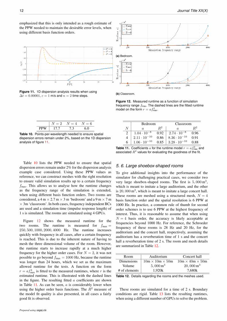
12 Journal Title XX(X)
emphasized that this is only intended as a rough estimate ofthe PPW needed to maintain the desirable error levels, whenusing different basis function orders.
Figure 11. 1D dispersion analysis results when using∆t = 0.00001, c = 1 m/s and n = 2 time steps.
N = 2 N = 4 N = 6PPW 17.7 7.3 6.0
Table 10. Points-per-wavelength needed to ensure spatialdispersion errors remain under 2%, based on the 1D dispersionanalysis of figure 11.
Table 10 lists the PPW needed to ensure that spatialdispersion errors remain under 2% for the dispersion analysisexample case considered. Using these PPW values asreference, we can construct meshes with the right resolutionto ensure valid simulation results up to a certain frequencyfmax. This allows us to analyse how the runtime changesas the frequency range of the simulation is extended,when using different basis function orders. Two rooms areconsidered, a 4 m× 2.7 m× 3 m ‘bedroom’ and a 9 m× 7 m× 3m ‘classroom’. In both cases, frequency independent BCsare used and a simulation time (impulse response length) of1 s is simulated. The rooms are simulated using 4 GPUs.
Figure 12 shows the measured runtime for thetwo rooms. The runtime is measured for fmax =250, 500, 1000, 2000, 4000 Hz. The runtime increasesquickly with frequency in all cases, after a certain frequencyis reached. This is due to the inherent nature of having tomesh the three dimensional volume of the room. However,the runtime starts to increase rapidly at a much higherfrequency for the higher order cases. For N = 2, it was notpossible to go beyond fmax = 1000 Hz, because the runtimewas longer than 24 hours, which we set as the maximumallowed runtime for the tests. A function on the formr = af4
max is fitted to the measured runtimes, where r is theestimated runtime. This is illustrated with the dashed linesin the figure. The resulting fitted a coefficients are shownin Table 11. As can be seen, a is considerably lower whenusing the higher order basis functions. The R2 measure ofthe model fit quality is also presented, in all cases a fairlygood fit is observed.
(a) Bedroom.
(b) Classroom.
Figure 12. Measured runtime as a function of simulationfrequency range fmax. The dashed lines are the fitted runtimemodel on the form r = af4
max.
Bedroom ClassroomN a R2 a R2
2 1.04 · 10−8 0.92 2.74 · 10−8 0.964 2.11 · 10−10 0.86 8.36 · 10−10 0.916 1.06 · 10−10 0.85 3.28 · 10−10 0.88
Table 11. Coefficients a for the runtime model r = af4max and
associated R2 values for evaluating the goodness of the fit.
5. 6. Large shoebox-shaped rooms
To give additional insights into the performance of thesimulator for challenging practical cases, we consider twovery large shoebox-shaped rooms. The first is 5, 000 m3,which is meant to imitate a large auditorium, and the otheris 20, 000 m3, which is meant to imitate a large concert hall.These rooms are meshed using a structured mesh, N = 4basis function order and the spatial resolution is 6 PPW at1000 Hz. In practice, a common rule of thumb for secondorder schemes is to use 6 PPW at the highest frequency ofinterest. Thus, it is reasonable to assume that when usingN = 4 basis order, the accuracy is likely acceptable atfrequencies beyond 1000 Hz. For reference, the Schroederfrequency of these rooms is 28 Hz and 20 Hz, for theauditorium and the concert hall, respectively, assuming theauditorium has a reverberation time of 1 s and the concerthall a reverberation time of 2 s. The room and mesh detailsare summarized in Table 12.
Room Auditorium Concert hallDimensions 10m× 10m× 50m 10m× 40m× 50m
Volume 5, 000 m3 20, 000 m3
# of elements 1,920k 7,680kTable 12. Details regarding the rooms and the meshes used.
These rooms are simulated for a time of 2 s. Boundaryconditions are rigid. Table 13 lists the resulting runtimes,when using a different number of GPUs to solve the problem.
Prepared using sagej.cls

Melander et al. 13
#GPUs Auditorium Concert hall1 6.52 −2 3.35 −4 1.82 7.238 1.02 4.4112 1.09 3.23
Table 13. Runtimes in hours for the large shoebox-shapedrooms.
For the auditorium case, the runtime improves signifi-cantly when increasing from 1 GPU to 8 GPUs. Using 12GPUs results in slightly worse performance compared tothe case of using 8 GPUs, indicating that communicationcosts between cores have begun to dominate. For the concerthall, the simulation cannot be run on 1 or 2 GPUs due tomemory limitations. For the higher GPU counts, the runtimedrops considerably as the number of GPUs is increased,and likely would drop further if more than 12 GPUs wereused. We have thus shown that for very large rooms, wecan simulate up to 30 times the Schroeder frequency withinpractical timeframes. However, one has to keep in mind thatthis simulation was run on structured meshes in a rectangularroom with rigid BCs. A more complex geometry, which hasto be meshed as an unstructured mesh, could lead to smallertime-steps and therefore longer runtime.
5. 7. Complex geometry cases
5. 7. 1. Auditorum B341-A21 at DTUAs an example of using the simulator on realistic 3Dgeometries, consider the room in Figure 13, which shows asimplified model of auditorium B341-A21 at the TechnicalUniversity of Denmark (DTU). As can be seen, the modelcontains a desk at the bottom and several benches on theslope. Boundary conditions have been chosen to representa realistic scenario, where the floor, table and benchesare set to be rigid, the walls have frequency independentimpedance boundary conditions with Z = 15, 630 Ns/m4,which corresponds to approximately 10% absorption atnormal incidence, and the ceiling uses frequency dependentboundary conditions. The ceiling is modeled as a suspendedporous material, with thickness dmat = 0.02 m, and air cavitydepth of d0 = 0.2 m and having flow resistivity σmat =50, 000 Ns/m4. The initial condition is a Gaussian pulsewith width sxyz = 0.3 m2, placed at S = (4.0, 5.0, 1.8) m,to mimic the position of a lecturer. Figure 14 presents aseries of snapshots of the solution in the XZ-plane at y = 5m, showing the propagation of the acoustic wave within thedomain. Note that the diffraction patterns from the benchesand the desk are being accurately captured.
5. 7. 2. Star-shaped room with a domeAs a last test case, consider the geometry shown in Figure15, which consists of three overlapping rectangles and adome shaped roof in the center. This geometry is meshedwith curvilinear elements to accurately capture the curvedshape of the dome. The geometry is similar to what isused in a work by Bilbao (6), however, in that work, thegeometry is meshed with affine elements and simulatedwith a second order accurate method. The floor is made
Figure 13. Geometric model of auditorium B341-A21 at DTU.
Figure 14. Snapshots of the acoustic wave propagating insidethe auditorium.
to be highly absorptive, having a normal incidence surfaceimpedance of Z = ρc = 411.6 Ns/m4, while other surfacesare perfectly reflecting. Figure 16 shows snapshots of thewave propagation in the room, both in a section view and aplan view. Note the acoustic focusing effect due to the dome.
The two complex geometry cases presented in this sectionand the previous one show that the simulator is capable ofusing the geometrical flexibility of the DGFEM method tosimulate realistic large-scale geometries.
6. ConclusionsA massively parallel nodal DGFEM-based room acousticsimulator has been presented and its performance analysed.It has been shown that the simulator can handle largeand complex problems, including curvilinear geometriesand frequency dependent boundaries, under short runtimes.This makes the simulator suited for use on problems
Prepared using sagej.cls

14 Journal Title XX(X)
Figure 15. Geometric model of dome shaped room.
Figure 16. Snapshots of the acoustic wave propagating insidethe star-shaped room.
of industrial size and complexity. The work presentedhere extends the usability of wave-based room acousticsimulations far beyond the restricted use-case of small roomsand frequencies below the Schroeder frequency, which wave-based methods are historically typically associated with.
The heterogeneous multi-device scalability benchmarksshow that the simulator can handle problems of nearly
arbitrary size, as long as the number of GPUs is selected toensure that the workload on each GPU is sufficient, to avoidcosts, related to communication between CPU cores startingto dominate the runtime. It is also shown that using mesh-adaptive high-order numerical methods is highly beneficialfor room acoustic simulations, due to the improved physicaldescription such wave-based rooom acoustic model offer.
Acknowledgements
The DTU Computing Center (DCC) supported the work with accessto state-of-the-art computing resources. The authors wish to thankMr. Hermes Sampedro Llopis and Mr. Nikolas Borrel-Jensen forfruitful discussions regarding this work.
References
[1] L. Savioja and U. P. Svensson. Overview of geometricalroom acoustic modeling techniques. J. Acoust. Soc. Am.,138(2):708–730, 2015.
[2] J. B. Allen and D. A. Berkley. Image method for efficientlysimulating small-room acoustics. J. Acoust. Soc. Am., 65:943–950, 1979.
[3] A. Krokstad, S. Strom, and S. Soersdal. Calculating theacoustical room response by the use of a ray tracing technique.J. Sound Vib., 8(1):118–125, 1968.
[4] D. Botteldooren. Finite-difference time-domain simulation oflow-frequency room acoustic problems. J. Acoust. Soc. Am.,98(6):3302–3308, 1995.
[5] M. Hornikx, T. Krijnen, and L. van Harten. openPSTD: Theopen source pseudospectral time-domain method for acousticpropagation. Comput. Phys. Comm., 203:298–308, 2016.
[6] S. Bilbao. Modeling of complex geometries and boundaryconditions in finite difference/finite volume time domain roomacoustics simulation. IEEE Trans. Audio, Speech, Lang. Proc.,21(7):1524–1533, 2013.
[7] J. A. Hargreaves, L. R. Rendell, and Y. W. Lam. A frameworkfor auralization of boundary element method simulationsincluding source and receiver directivity. J.Acoust. Soc. Am.,145(4):2625–2637, 2019.
[8] A. Craggs. A finite element method for free vibration ofair in ducts and rooms with absorbing walls. J. Sound Vib.,173(4):568–576, 1994.
[9] F. Pind, A. P. Engsig-Karup, C. H. Jeong, J. S. Hesthaven,M. S. Mejling, and J. Strømann Andersen. Time domain roomacoustic simulations using the spectral element method. J.Acoust. Soc. Am., 145(6):3299–3310, 2019.
[10] H. Wang, I. Sihar, R. Pagan Munoz, and M. Hornikx.Room acoustics modelling in the time-domain with thenodal discontinuous Galerkin method. J. Acoust. Soc. Am.,145(4):2650–2663, 2019.
[11] H.-O. Kreiss and J. Oliger. Comparison of accurate methodsfor the integration of hyperbolic equations. Tellus, 24(3):199–215, 1972.
[12] J. J. Lopez, D. Carnicero, N. Ferrando, and J. Escolano.Parallelization of the finite-difference time-domain methodfor room acoustics modelling based on cuda. Math. Comput.Mod., 57(7):1822–1831, 2013.
[13] C. Spa, A. Rey, and E. Hernandez. A GPU implementation ofan explicit compact FDTD algorithm with a digital impedance
Prepared using sagej.cls

Melander et al. 15
filter for room acoustics applications. IEEE/ACM Trans.Audio, Speech, Lang. Proc., 23(8):1368–1380, 2015.
[14] T. Takahashi and T. Hamada. GPU-accelerated boundaryelement method for Helmholtz’ equation in three dimensions.Int. J. Num. Methods Eng., 80(10):1295–1321, 2009.
[15] N. Morales, R. Mehra, and D. Manocha. A parallel time-domain wave simulator based on rectangular decompositionfor distributed memory architectures. Applied Acoustics,97:104–114, 2015.
[16] D. S. Medina, A. St-Cyr, and T. Warburton. OCCA: A unifiedapproach to multi-threading languages, 2014. Article preprint.
[17] D. Dragna, P. Pineau, and P. Blanc-Benon. A generalizedrecursive convolution method for time-domain propagation inporous media. J. Acoust. Soc. Am., 138(2):1030–1042, 2015.
[18] J. S. Hesthaven and T. Warburton. Nodal DiscontinuousGalerkin Methods – Algorithms, Analysis, and Applications.Springer, New York, 2008. Ch. 3.
[19] J. S. Hesthaven and C. H. Teng. Stable spectral methods ontetrahedral elements. SIAM J. Sci. Comput., 21(6):2352–2380,2000.
[20] M. Ainsworth. Dispersive and dissipative behaviour of highorder discontinuous Galerkin finite element methods. J.Comput. Phys., 198(1):106–130, 2004.
[21] F. Hu and H. Atkins. Two-dimensional wave analysis ofthe discontinuous Galerkin method with non-uniform gridsand boundary conditions. In 8th AIAA/CEAS AeroacousticsConference Exhibit, 2002.
[22] F. T. Eleuterio. Riemann Solvers and Numerical Methods forFluid Dynamics: A Practical Introduction. Springer-Verlag,2. edition, 1999.
[23] M.H. Carpenter and C. Kennedy. Fourth-order 2N-storageRunge-Kutta schemes. NASA report TM 109112, NASALangley Research Center, 1994.
[24] A.P. Engsig-Karup, C. Eskilsson, and D. Bigoni. A stabilisednodal spectral element method for fully nonlinear waterwaves. J. Comput. Phys., 318:1–21, 2016.
[25] C. A. Kennedy and M. H. Carpenter. Additive Runge-Kuttaschemes for convection-diffusion-reaction equations. Appl.Num. Math., 44(1):139–181, 2003.
[26] H. Wang, J. Yang, and M. Hornikx. Frequency-dependenttransmission boundary condition in the acoustic time-domain nodal discontinuous Galerkin model. Appl. Acoust.,164:107280, 2020.
[27] C. Geuzaine and J.-F. Remacle. Gmsh: a three-dimensionalfinite element mesh generator with built-in pre- and post-processing facilities. Int. J. Num. Methods Eng., 79(11):1309–1331, 2009.
[28] J.S. Hesthaven. From electrostatics to almost optimal nodalsets for polynomial interpolation in a simplex. SIAM J. Num.Analysis, 35(2):655–676, 1998.
[29] A. Karakus, N. Chalmers, K. Swirydowicz, and T. Warburton.A GPU accelerated discontinuous Galerkin incompressibleflow solver. J. Comput. Phys., 390:380–404, 2019.
[30] K. Swirydowicz, N. Chalmers, A. Karakus, and T. Warburton.Acceleration of tensor-product operations for high-order finiteelement methods. Int. J. High Perf. Comput. Appl., 33(4):735–757, 2019.
[31] S. Sakamoto. Phase-error analysis of high-order finitedifference time domain scheme and its influence on
calculation results of impulse response in closed sound field.Acoust. Sci.Tech., 28(5):295–309, 2007.
[32] A.P. Engsig-Karup, C. Eskilsson, and D. Bigoni. A stabilisednodal spectral element method for fully nonlinear waterwaves. J. Comp. Physics., 318:1–21, 2016.
[33] R. M. Kirby and G. E. Karniadakis. De-aliasing on non-uniform grids: algorithms and applications. J. Comput.Physics, 191(1):249–264, 2003.
[34] S.-I. Thomasson. Reflection of waves from a point source byan impedance boundary. J. Acoust. Soc. Am., 59(4):780–785,1976.
[35] Y. Miki. Acoustical properties of porous materials—modifications of Delany-Bazley models. J. Acoust. Soc. Jap.,11(1):19–24, 1990.
[36] J. F. Allard and N. Atalla. Propagation of Sound in PorousMedia: Modelling sound absorbing materials. Wiley, WestSussex, United Kingdom, 3rd edition, 2009. Ch. 3,5.
[37] B. Gustavsen and A. Semlyen. Rational approximation offrequency domain responses by vector fitting. IEEE Trans.Pow. Del., 14(3):1052–1061, 1999.
[38] J. Saarelma, J. Botts, B. Hamilton, and L. Savioja. Audibilityof dispersion error in room acoustic finite-difference time-domain simulation as a function of simulation distance. J.Acoust. Soc. Am., 139(4):1822–1832, 2016.
Prepared using sagej.cls

PAPER P6
134

Experimental validation and uncertainty quantification in wave-based computationalroom acoustics
Tobias Thydala,∗, Finnur Pinda,b, Cheol-Ho Jeonga, Allan P. Engsig-Karupc
aAcoustic Technology, Department of Electrical Engineering, Technical University of Denmark, 2800 Kgs. Lyngby, DenmarkbHenning Larsen, 1620 Copenhagen, Denmark
cDepartment of Applied Mathematics and Computer Science, Technical University of Denmark, 2800 Kgs. Lyngby, Denmark
Abstract
It is well known that input data uncertainty has a major influence on the correctness of room acoustic simulations. Thispaper proposes a comprehensive framework for experimental validation and uncertainty quantification in room acousticsimulations. The sources of uncertainty in room acoustic simulations are many, but especially the boundary conditionspresent significant uncertainty. The input data uncertainty is propagated through the simulation model, which in thiswork is a wave-based time-domain discontinuous Galerkin finite element method (DGFEM) simulation scheme, andis then presented as a ‘probability box’ (p-box), expressing both aleatory and epistemic input data uncertainties andmodel form uncertainties. The p-box can then be compared against the perceptual limits of the human auditory systemto gauge the severity of the uncertainty. The framework is applied on a small room with an absorbing wall for theexperimental validation of the simulation results and the uncertainty quantification of three boundary parameters: theflow resistivity of the porous absorber, the thickness of the porous absorber, and the absorption characteristics of theremaining hard walls. It is found that the input data uncertainty and the model form uncertainty are too high for themodel to be able to predict several room acoustic parameters within just noticeable thresholds.
Keywords: Uncertainty quantification, experimental validation, wave-based room acoustic simulations, porous soundabsorbers
1. Introduction
Room acoustic simulations, first proposed by Schroederet al. in 1962 [1], are used, e.g., for research, building de-sign and virtual entertainment. The reliability of the sim-ulations depends very much on the skills of the operator,who creates a geometrical model and assigns input datafor simulations, including boundary conditions [2]. Partic-ularly when using geometrical acoustic (GA) simulationmethods, such as the image source method [3] or the raytracing method [4], the users’ skills have a major influencewhen making computer-aided design (CAD) polygon mod-els with adequate levels of detail [5, 6, 7, 8]. Fine-grainedgeometrical details are replaced with planar surfaces andassigned scattering coefficients, which are often based oncrude visual inspection [9]. Wave-based simulation meth-ods on the other hand, particularly those methods that canbe formulated to operate on unstructured meshes, such asthe finite element method [10] and the boundary elementmethod [11], are able to use much more detailed geomet-rical models, thereby reducing the uncertainty associatedwith the geometrical modeling.
In addition to the uncertainty caused by geometricalsimplification, absorption properties used in room acoustic
∗Corresponding authorEmail address: [email protected] (Tobias Thydal)
simulations also introduce uncertainty in the input data.During the design stage, it is unlikely that the exact ab-sorption properties of the surface boundaries are known.In an existing building too, the acoustic properties of theboundary surfaces are hard to obtain and in most cases,reliable in-situ measurements cannot be made.
Despite the well-known fact that uncertainties in inputparameters have a major influence on the correctness ofroom acoustic simulations, the uncertainty quantificationof such room acoustic simulations has not been studiedwidely. Vorlander claimed a great need for this topic tobe investigated and presented the latest findings using thefundamental concept of error propagation [2]. It is worthnoting that the Guide to the Expression of Uncertainty inMeasurements (GUM) has been widely used in uncertaintyquantification of room acoustic measurements [12, 13].
In this paper, we propose to use the comprehensiveframework of Roy and Oberkampf [14, 15] as a means tovalidate and estimate the uncertainty of wave-based roomacoustic simulations. We apply the comprehensive valida-tion and uncertainty quantification (VUQ) framework toa simple test case of a small rectangular room with twotypes of boundaries: bare concrete walls on five of thesurfaces, and with the sixth surface being covered by aporous material mounted on rigid backing. Previous workhas indicated that this type of room is particularly diffi-
Preprint submitted to Journal of Applied Acoustics July 2, 2020

cult to simulate with high precision [16]. Experiments arecarried out to serve as a ground truth reference, which thesimulations are compared against. The main sources of un-certainty in our investigation are the flow resistivity of theporous absorber, the thickness of the porous absorber, andthe absorption coefficients of the bare concrete walls. Theuncertainty in the T30, EDT, D50 and C80 room acousticparameters is estimated [17].
The paper is organised as follows. In Sec. 2 the gen-eral framework is presented with descriptions of the stepsinvolved. Furthermore, the input data uncertainties areidentified and described. Sec. 3 describes the experimen-tal setup and Sec. 4 introduces the wave-based simulationmodel. In Sec. 5 the results are presented and discussed,and, finally, some concluding remarks are offered in Sec. 6.
2. Validation and uncertainty quantificationframework
The VUQ framework allows for the propagation of bothaleatory and epistemic uncertainty in the input data andcombines the results into one analysis. The analysis yieldsa validation metric that is capable of dealing with caseswhere few simulation and/or measurement data points areavailable. This is particularly useful in wave-based roomacoustics simulations, where long computation times pro-hibit the collection of large data sets.
The general workflow consists of three parts: i) the val-idation experiment, ii) the simulations and iii) the valida-tion and uncertainty quantification of the simulation dataagainst the experimental data. A flowchart of the overallprocedure is shown in Fig. 1.
Figure 1: Flowchart of the overall validation and uncertainty quan-tification procedure proposed by Oberkampf and Roy. Adapted from[14].
The first step, the validation experiment, involves col-lecting the required measurement data for comparisonwith the simulation, which in the case of room acousticstypically entails impulse response measurements, accord-ing to ISO 3382-2 [18]. During the measurement process,
all model inputs, including boundary conditions, initialconditions, geometry, physical parameters and the sys-tem excitation, must be identified and characterised. Thischaracterisation includes classifying whether the input un-certainties are deterministic, aleatory or epistemic, as wellas noting the relevant properties for each model input,such as the flow resistivity of a porous absorber, which isa primary factor for representing the absorption coefficientof the porous absorber.
Aleatory uncertainties arise due to inherent randomnessin the model input, e.g., the random arrangement of fi-bres/pores in porous absorbers, and it should therefore bedescribed by either a probability density function or a cu-mulative distribution function (CDF). The common wayto propagate aleatory uncertainty through the simulationmodel is by using Monte Carlo sampling, which requires alarge number of samples to accurately capture low proba-bility events. More advanced techniques can be used, suchas polynomial chaos expansion, to reduce the number ofsamples required [19, 20].
Epistemic uncertainty arises due to lack of knowledgeabout a model input, which can be due to limitations in themeasurement equipment used to measure the model inputsor a simplifying assumption about the model input. Dueto the lack of knowledge about epistemic uncertainty val-ues, it is most reasonable to assume that the model inputhas a uniform probability over an interval. The bounds ofthe interval are typically guessed from the limited knowl-edge available and/or defined based on experience. Anexample of epistemic uncertainty could be the thickness ofan absorber where only the manufacturing tolerances areknown. These tolerances mark the bounds of the intervalof values possible, but there is no further knowledge of thedistribution or likelihood of values within that interval.
The second step involves propagating the model inputscharacterised during the first step through the simulationmodel. If the uncertainty is purely aleatory, the propa-gation of the model input results in a CDF. For purelyepistemic uncertainty it results in a set of values withinan interval. If the uncertainty has both aleatory and epis-temic characteristics, it will result in a set of CDFs spreadover an interval. Generally the two outermost CDFs aremost important, as they denote the bounds of the sim-ulation output space and together form a probability box(p-box). The p-box is compared against the measurementdata from the experiment using a validation metric thatquantifies any potential deviation of the simulation resultsfrom the experimental results.
2.1. Sources of uncertainty in the boundary conditions
Three of the model inputs pertaining to the boundaryconditions of the small room test case are identified to beuncertain and therefore investigated in this study: the flowresistivity of the absorber (aleatory), the thickness of theabsorber (epistemic) and the absorption coefficient of theconcrete wall (epistemic).
2

2.1.1. Flow resistivity
The flow resistivity, σ, is an aleatory uncertainty due tothe inherent randomness in the distribution, orientationand dimensions of the fibres. In this work we use Miki’smodel to estimate the characteristic impedance and propa-gation constant of the porous material for the simulations,based on the material’s flow resistivity [21]. The charac-teristic impedance is given by
Zc(f) = 1 + 0.070
(f
σ
)−0.632− j0.107
(f
σ
)−0.632, (1)
and the propagation constant is given by
γ(f) =2πf
c
[0.16
(f
σ
)−0.618]
+ j2πf
c
[1 + 0.109
(f
σ
)−0.618],
(2)
where f is the frequency in Hz and c is the speed of soundin air. The flow resistivity values are sampled from a nor-mal distribution using the Monte Carlo sampling scheme.In this study two different porous absorbers are consid-ered. One of the absorbers is an Ecophon Akusto Wall A40 mm glass wool porous absorber (A1) and the other isan Ecophon Industry Modus 100 mm glass wool porous ab-sorber (A2). The flow resistivity mean is 47,000 k Pa s/m2
and 10,900 k Pa s/m2 for A1 and A2, respectively. Thestandard deviation is 5,875 k Pa s/m2 and 1,363 k Pa s/m2
for A1 and A2, respectively. The values are obtained fromthe producer of the materials, Saint-Gobain Ecophon.
2.1.2. Thickness
The thickness of the porous absorber contains uncer-tainty due to manufacturing tolerances. It is used in con-junction with the characteristic impedance when calculat-ing the normal surface impedance of the porous absorber[22],
Z(f, θ) = −jZc(k/kx) cot(kxd), (3)
where θ is the angle of the incident wave, k is the wave-number of the porous absorber, kx is the wave-number inthe x-direction normal to the porous absorber and d isthe thickness of the porous absorber. We assume that theporous absorber is locally reacting, which simplifies themodel and is generally taken to be an acceptable approx-imation when the porous absorber is mounted on a rigidbacking and has a high flow resistivity [23]. The thicknessis modelled as an epistemic uncertainty where the manu-facturing tolerances mark the upper and lower bound in astatistical sense. The tolerances specified by Ecophon are±3 mm.
2.1.3. Surface impedance of the concrete walls
The surface impedance of the concrete walls is deter-mined based on random incidence absorption coefficientsfound in the literature which are converted to the locally
reacting, real valued surface impedance using the followingformula [24],
αrandom = 81
z
(1− 1
z· ln(1 + 2z + z2) +
1
1 + z
), (4)
where αrandom is the random incidence absorption coeffi-cient, z = Z/Z0, where Z0 is the characteristic impedanceof air, c is the speed of sound and ρ is the density of air(c = 343 m/s and ρ = 1.2 kg/m3 in this work). Because therandom incidence absorption coefficients of concrete wallsvaries in the literature, it is modelled as an epistemic un-certainty. In this work, the bounds are taken to be 0.029and 0.048 for the 125 Hz and 250 Hz octave bands and0.043 and 0.071 for the 500 Hz octave band. This corre-sponds to a surface impedance range of 109 k Ns/m4 to65 k Ns/m4 for the 125 Hz and 250 Hz octave bands and72 k Ns/m4 to 43 k Ns/m4 for the 500 Hz octave band.Since the absorption coefficients are only known in octavebands, and the surface impedance is made to be a contin-uous function over frequency using a linear interpolation.
2.2. System response quantities
Four output system response quantities (SRQs) are cho-sen based on their common use in the room acousticsfield, and due to them having documented just-noticeable-difference (JND) values. The JNDs are especially impor-tant as they provide perceptual limits that mark whetherthe model predicts the system response quantities withsufficient accuracy. This means that as long as the modelpredicts the SRQs within the JND limits, there will beno audible differences between the simulation and the realworld case. The four SRQs are the reverberation time T30[s], the early decay time EDT [s], definition D50 [dimen-sionless ratio] and clarity C80 [dB], as they are defined inISO 3382[17].
2.3. Validation metric
The validation metric used in this work is the MinkowskiL1 metric [25], which describes the area between two dis-tributions,
d(F, S) =
∫ ∞
−∞|F (x)− S(x)|dx, (5)
where F is the CDF of the simulated results and S isthe CDF of the measurement results. This metric worksregardless of the number of data points there are in thesimulation data set or the measurement data set, and itprovides a measure of the disagreement between the simu-lation results and the measurement results. Furthermore,d has the same unit as the analysed SRQ, which givesa more intuitive representation of the potential differencebetween the simulated and measured results.
Figure 2 shows two graphs where the blue vertical linesindicate a single experimental data point and the blacklines indicate the probability boxes of the simulation re-sults. The left graph shows a case where the model is
3

validated because the simulation fully captures the mea-surement data, which is numerically represented by an areavalidation metric d = 0. The right graph show that thesimulation data does not fully capture the measurementdata and therefore has d > 0, as indicated by the grayshaded area.
Figure 2: Examples of a p-box where the black lines indicate thep-box, the blue vertical line indicates a measurement data point andthe grey area is the area validation metric. Adapted from [15]
When the model is unable to predict the measurementdata with the given model input uncertainty, d > 0, itindicates that the model itself contains uncertainty whichOberkampf and Roy label model form uncertainty. Dif-ferent factors can introduce model form uncertainty, suchas assumptions or simplifications made in the model. Thearea validation metric allows for the inclusion of the modelform uncertainty by appending the value of d to either sideof the p-box, meaning that the left CDF has the value ofd subtracted from all its data points and the right CDFhas the value of d added to all its data points. By ap-pending the value of d to both sides of the p-box, it willrepresent the total uncertainty of the simulations by in-cluding both the model input uncertainty and the modelform uncertainty.
Because the four proposed SRQs have well documentedJNDs, we propose an additional step to check whether theuncertainty in the model presents perceptible deviationsfrom the measured data. By appending the JND of theSRQ to either side of the measured data we obtain somelimits that denote how much the simulation results areallowed to deviate from the measured data without in-troducing perceptible differences. This will be discussedfurther in Sec. 5.
3. Validation experiment
The impulse response measurements are performed in asmall rectangular room with the dimensions (4.38, 3.27,3.29) m, shown in Fig. 3. All six surfaces in the roomare painted concrete surfaces, with one surface containing
a heavy steel door. One of the vertical surfaces is coveredby the porous absorber, so the room consists of five hardwalls and one absorptive surface.
Figure 3: Photograph of the room being measured with the 100 mmporous absorber mounted on the end wall.
Two source positions and two receiver positions areused, resulting in four different source-receiver combina-tions. The impulse response measurements are performedin accordance with ISO3382-2 [18], except for the source 1position, which is intentionally placed in the corner to testthe capabilities of the simulation model. Figure 4 shows atop down view of the room used, with the dots and circlesdenoting the sources and receivers, respectively, and thethick left vertical line representing the porous absorber.
x-axis
y-axis
S1
S2
R1R2
Figure 4: Top down view of the room. The red dots represent thesource positions, the blue circles represent the microphones and thethick vertical left line represents the sound absorber boundary.
4

4. Discontinuous Galerkin finite element methodscheme
An in-house time-domain discontinuous Galerkin finiteelement method (DGFEM) room acoustic simulation toolis used to carry out all simulations conducted in this work.The simulator solves the following set of partial differentialequations that describe wave motion in a lossless medium,
vt = −1
ρ∇p,
in Ω,
pt = −ρc2∇ · v,(6)
where v(x, t) is the particle velocity, p(x, t) is the soundpressure, x is the position in the air domain Ω and t is time.The implementation of the simulator follows the quadra-ture free nodal approach described in Ref. [26]. The readeris referred to this reference for an in-depth description ofthe numerical method. The spatial domain Ω is dividedinto a set of geometrically conforming elements Dk, i.e.,Ω ≈ (Ω)h =
⋃Kk=1D
k, where K is the total number ofelements in the mesh and h denotes the numerical approx-imation. In this work, unstructured meshes of tetrahedralelements are used in all simulations. On each element, thelocal solution is represented as a nodal polynomial seriesexpansion using Lagrange basis functions of order N . Ap-plying a Galerkin projection and integration by parts twiceon the governing equations yields the strong formulation
∫
Dk
∂vkh
∂t`kn dx = −1
ρ
∫
Dk
∇pkh`kn dx
+1
ρ
∫
∂Dk
n · (pkh − p∗)`kn dx,∫
Dk
∂pkh∂t
`kn dx = −ρc2∫
Dk
∇ · vkh`
kn dx
+ ρc2∫
∂Dk
n · (vkh − v∗)`kn dx,
(7)
where `kn are the nodal basis functions and the star-labeledterms denote the numerical flux terms that account for thecoupling between elements. In this work, an upwind nu-merical flux is employed. Inserting the polynomial seriesexpansions into the strong formulation leads to the follow-ing semi-discrete system
Mk dukh
dt= −1
ρSkxpkh +
1
ρEknx(pkh − p∗),
Mk dvkh
dt= −1
ρSky pkh +
1
ρEkny(pkh − p∗),
Mk dwkh
dt= −1
ρSkz pkh +
1
ρEknz(pkh − p∗),
Mk dpkh
dt= −ρc2(Skxukh + Sky vkh + Skzwk
h)
+ ρc2Ekn · (vkh − v∗),
(8)
where u, v, w are the x, y, z components of the particlevelocity, Mk ∈ RNp×Np is the local mass matrix, Sk ∈
RNp×Np is the local stiffness matrix and Ek ∈ RNp×4Nfp ,is a matrix operator for carrying out the surface integra-tion. Np is the number of nodes per element and Nfp
is the number of nodes on a single element face. Thesemi-discrete system in Eq. 8 is integrated in time usinga low-storage 4th order explicit Runge-Kutta time step-ping method [27]. Surface impedance boundary conditionsare weakly enforced through the numerical flux terms. Toaccount for locally-reacting frequency dependent surfaceimpedance, the method of auxiliary differential equations,as described in Ref. [28], is used.
5. Results and discussion
Simulated and measured frequency responses are shownin Figs. 5 and 6. By visual inspection, a good agreementbetween measurements and simulations is observed. Thisindicates that the model is capable of capturing the acous-tical behaviour of the room, however, with some deviationsin the response level, which are likely attributed to impre-cise boundary conditions.
Figure 5: Transfer function of the room with the 100 mm porousabsorber installed and using source 1 and receiver 1.
Figure 6: Transfer function of the room with the 40 mm porousabsorber installed and using source 2 and receiver 2.
Moving to the time domain we get more mixed results,as the model does well in simulating T30 but struggles morewith the other SRQs, as shown in Table 1 and Table 2. Theresults are fairly similar for both porous absorbers.
5

S1R1 S1R2 S2R1 S2R240 mm Akusto Wall A
T30
125 Hz 0.01 0.03 0 0250 Hz 0 0 0.04 0500 Hz 0 0 0 0
EDT125 Hz 0.24 0.01 0.07 0.250 Hz 0 0.03 0.01 0.03500 Hz 0 0.1 0 0
D50 100-630 Hz 0 0.12 0.01 0.10C80 100-630 Hz 0 1.1 0 0
Table 1: Area validation metric, d, for the four SRQs at the foursource-receiver positions for the 40 mm porous absorber.
S1R1 S1R2 S2R1 S2R2100 mm Industry Modus
T30
125 Hz 0 0 0 0250 Hz 0.64 0 0.42 0500 Hz 0 0 0 0
EDT125 Hz 0 0.26 0.1 0.06250 Hz 0 0.05 0 0.11500 Hz 0 0 0 0
D50 100-630 Hz 0 0.13 0.7 0.9C80 100-630 Hz 0 1.92 0.2 0.25
Table 2: Area validation metric, d, for the four SRQs at the foursource-receiver positions for the 100 mm porous absorber.
In Fig. 7, all the CDFs calculated for the T30 parameterin the 125 Hz, 250 Hz and 500 Hz octave bands are shown,for the S2R2 case with the 40 mm porous absorber. In eachoctave band, three sets of CDFs are presented, with eachset consisting of two CDFs. The first set is shown withdashed lines, representing the lower and upper bound ofthe porous material thickness, when the absorption at theconcrete walls is at the lower bound. The second set isshown with solid lines, representing the lower and upperbound of the porous material thickness, when the absorp-tion at the concrete walls is at the mean value. The lastset is shown with dotted lines, representing the lower andupper bound of the porous material thickness, when theabsorption at the concrete walls is at the upper bound.
A visual inspection of the CDFs shown in Fig. 7 can beused to get an idea of which of the three uncertain bound-ary conditions has the greatest impact on the uncertaintyin the T30. For the epistemic uncertainties (thickness andconcrete wall absorption), the impact of the uncertainty isgiven by the distance between the different CDFs. For thealeatory uncertainty (flow resisitivity), the slope of the in-dividual CDFs indicates the uncertainty, where a steeperslope is related to the uncertainty having a smaller impacton the SRQ. It is evident that the absorption propertiesof the hard walls are the most significant cause of uncer-tainty in the simulation. However, the uncertainty of thethickness of the absorber is also seen to have a consider-able influence at lower frequencies, particularly in the 125Hz octave band.
Figure 7: All T30 CDFs for the for the 40 mm porous absorber caseusing source 2 and receiver 2.
It is from these sets of CDFs that the two outermostCDFs for each octave band are selected to designate thep-box of the SRQ. Figure 8 shows the p-boxes, for thissame case (S2R2, 40 mm, T30). This is an example of avalidated case, where the T30 p-boxes in the 125 Hz, 250 Hzand 500 Hz octave bands fully encapsulate the measure-ment data, indicating that the model is sufficiently accu-rate given the input uncertainty, i.e., the model form un-certainty is within acceptable limits. However, it is evidentthat the simulation results span a wide range of possibleT30, e.g., from approximately 1.5 s to approximately 2.7 sfor the 125 Hz octave band, which is due to the consider-able uncertainty in the input data. This is not necessarilyan issue if the span is within the perceptible limits of thehuman auditory system. To test whether that is the case,one JND is appended to either side of the measurementdata point. Clearly, the input data uncertainty introducestoo much output variability for the model to be able topredict this SRQ with a level of accuracy that is audiblyindistinguishable from the measurement data. This indi-cates that the current model input uncertainty must bereduced before the model can accurately predict T30 inthe room under test.
Figure 9 shows the probability boxes for the definitionparameter for all source-receiver combinations. In gen-eral, the model captures the measurement data better forreceiver 2 than receiver 1. This applies to the other SRQsas well. This difference between receivers could possiblybe explained by the fact that receiver 2 is closer to the
6

Figure 8: T30 p-boxes for the 40 mm porous absorber case usingsource 2 and receiver 2.
porous absorbing surface than receiver 1, and is thereforemore susceptible to inaccuracies in the modeling of theporous absorber, e.g., due to the local-reaction assump-tion.
Figure 10 shows a case where the model is incapableof predicting the measurement data with the given modelinput uncertainty. This means that the model form alsointroduces some uncertainty. A measure of the disagree-ment between the measured and simulated data is given bythe area validation metric d. The model form uncertaintyis included by appending the value of d to either side of thep-box, resulting in the p-box marked by the dashed line inFig. 10, which indicates the total uncertainty in the sim-ulation results. Again this p-box is compared against themeasured data with one JND appended, and it is foundthat the simulation results present perceptible differencesfrom the measured data.
The area validation metric can be used as a tool to iden-tify potential issues with the model form, if a varied se-lection of SRQs are utilised. Looking at both Table 1 and2, we see that the model is generally able to predict T30,as shown by d = 0, and it shows minor deviation for C80.However, for almost all source-receiver combinations, themodel struggles with both EDT and D50. Since both ofthese SRQs are heavily influenced by the early reflectionsto a greater extent than C80 and especially T30, whichare more influenced by the late reflections, it could po-tentially indicate that the model struggles to accuratelysimulate the early reflections. A potential reason for the
Figure 9: Definition for the 40 mm porous absorber case at the foursource-receiver combinations. Top-left is S1R1, top-right is S1R2,bottom-right is S2R1 and bottom-left is S2R2.
Figure 10: P-box of the Definition for the 40 mm absorber at S2R2.
inability to accurately simulate the early reflections mightbe due to the simplified surface impedance of the con-crete walls. Because we use random incidence absorptioncoefficients given in octave band increments to calculatethe continuous surface impedance of the concrete walls,we lack both proper frequency resolution as well as phaseinformation about the surface impedance. With five outof six surfaces being concrete walls, small deviations be-tween the true value and the value used in the simulationswill have a large impact on the results. Another reasoncould be because all surfaces are modeled as locally react-ing, which causes errors particularly for grazing incidencewaves, which might be more pronounced in the early re-flections for certain source-receiver positions, e.g., S1R2 inTable 1.
7

6. Conclusion
In this paper, a framework for the validation and uncer-tainty quantification of room acoustic simulation models ispresented. The framework is able to include both aleatoryand epistemic uncertainties, which are propagated throughthe simulation model, resulting in a p-box that capturesthe model input uncertainty. The framework is also capa-ble of capturing model form uncertainty by using an areavalidation metric, and then include that with the modelinput uncertainty to provide the total overall uncertaintyof the simulation results. This uncertainty can then becompared against the perceptual limits of the human earin order to gauge the severity of the uncertainty. Finally,the framework can serve as a tool to identify problematicapproximations in the input data and in the simulationmodel.
The framework is applied on a small rectangular roomtest case. Experimental data is compared against sim-ulation results from a wave-based DGFEM room acous-tic simulation model, with input uncertainties propagatedthrough the simulation model using the VUQ framework.It is found that the input data uncertainty is too high forthe model to be able to accurately predict common roomacoustic parameters within JND thresholds. For the T30and C80 parameters, the model form is validated in mostcases (d = 0), as the measurement data is completely en-compassed by the output variability caused by the inputdata uncertainty, as indicated by the p-box. Nevertheless,the variability is larger than the JND thresholds, meaningthat the input data uncertainty must be reduced beforethe model can predict these parameters with sufficient ac-curacy. The crude approximation of the absorption prop-erties of the concrete walls and the thickness tolerances ofthe porous materials are identified as large sources of un-certainty. For the EDT and D50 parameters, even largeruncertainties are seen, as the p-box does not encompassthe measurement data (d > 0), indicating shortcomings ofnot only the input data, but also in the model itself. Thelack of extended-reaction surface modeling is identified asa potential reason for these model form uncertainties.
References
[1] M. R. Schroeder, B. S. Atal, C. Bird, Digital computers in roomacoustics, Proc. 4th Int. Conf. Acoust. (1962) M21.1–M21.4.
[2] M. Vorlander, Computer simulations in room acoustics: Con-cepts and uncertainties, J. Acoust. Soc. Am. 133 (3) (2013)1203–1213.
[3] J. B. Allen, D. A. Berkley, Image method for efficiently simu-lating small-room acoustics, J. Acoust. Soc. Am. 65 (4) (1979)943–950.
[4] A. Krokstad, S. Strom, S. Sørsdal, Calculating the acousticalroom response by the use of a ray tracing technique, J. SoundVib. 8 (1) (1968) 118–125.
[5] L. Savioja, U. P. Svensson, Overview of geometrical room acous-tic modeling techniques, J. Acoust. Soc. Am. 138 (2) (2015)708–730.
[6] L. M. Wang, J. Rathsam, S. Ryherd, Interactions of model de-tail level and scattering coefficients in room acoustic computersimulation, in: Proc. Int. Symp. Room Acoust. (ISRA), 2004.
[7] T. Ziegler, Comparing measurement and simulation results us-ing model calibration for room acoustical evaluation of industryhalls, in: Proc. Euronoise, 2018.
[8] C. L.Christensen, G. B. Nielsen, J. H. Rindel, Danish acousticalsociety round robin on room acoustic computer modelling, Tech.rep. (2008).
[9] P. D’Antonio, T. J. Cox, Acoustic absorbers and diffusers: the-ory, design, and application, Taylor & Francis, Oxfordshire,2009.
[10] A. Craggs, A finite element method for free vibration of air inducts and rooms with absorbing walls, J. Sound Vib. 173 (4)(1994) 568–576.
[11] S. Kirkup, The boundary element method in acoustics: A sur-vey, Appl. Sci. 9 (8) (2019) 1642.
[12] P. Dietrich, Modeling measurement uncertainty in room acous-tics, Acta Polytech. 47 (4-5) (2007) 63–67.
[13] I. Witew, M. Vorlander, Uncertainties of room acousticalmeasurements—influence of the exact source and receiver po-sition, in: Proc. Inst. Acoust., 2011.
[14] W. L. Oberkampf, C. J. Roy, Verification and validation inscientific computing, Cambridge University Press, Cambridge,2011.
[15] C. J. Roy, W. L. Oberkampf, A comprehensive framework forverification, validation and uncertainty quantification in scien-tific computing, Comput. Meth. Appl. Mech. Eng. 200 (2011)2132–2144.
[16] G. Marbjerg, J. Brunskog, C.-H. Jeong, The difficulties of sim-ulating the acoustics of an empty rectangular room with anabsorbing ceiling, Appl. Acoust. 141 (2018) 35–45.
[17] Acoustics - Measurement of room acoustic parameters - Part 1:Performance spaces, Standard ISO 3382-1:2009, InternationalOrganization for Standardization, Geneva, CH (2009).
[18] Acoustics - Measurement of room acoustic parameters - Part2: Reverberation time in ordinary rooms, Standard ISO 3382-2:2008, International Organization for Standardization, Geneva,CH (2008).
[19] H. N. Najm, Uncertainty quantification and polynomial chaostechniques in computational fluid dynamics, Ann. Rev. FluidMech. 41 (1) (2009) 35–52.
[20] M. S. Eldred, Recent advances in non-intrusive polynomialchaos and stochastic collocation methods for uncertainty analy-sis and design, in: 50th AIAA/ASME/ASCE/AHS/ASC Struc-tures, Structural Dynamics, and Materials Conference, 2009.
[21] Y. Miki, Acoustical properties of porous materials – Generaliza-tions of empirical models, J. Acoust. Soc. Jap. 11 (1990) 25–28.
[22] J. F. Allard, N. Atalla, Propagation of Sound in Porous Media:Modelling sound absorbing materials, 3rd Edition, Wiley, WestSussex, 2009.
[23] M. Aretz, M. Vorlander, Efficient modelling of absorbing bound-aries in room acoustic FE simulations, Acta Acust. Acust. 96 (6)(2010) 1042–1050.
[24] M. Aretz, M. Vorlander, Combined wave and ray based roomacoustic simulations of audio systems in car passenger compart-ments, Part I: Boundary and source data, Appl. Acoust. 76(2014) 82–99.
[25] S. Ferson, W. L. Oberkampf, L. Ginzburg, Model validation andpredictive capability for the thermal challenge problem, Com-put. Meth. Appl. Mech. Eng. 197 (29-32) (2008) 2408–2430.
[26] J. S. Hesthaven, T. Warburton, Nodal Discontinuous GalerkinMethods—Algorithms, Analysis, and Applications, Springer,New York, 2008.
[27] M. Carpenter, C. Kennedy, Fourth-order 2N-storage Runge-Kutta schemes, NASA report TM 109112, NASA Langley Re-search Center (1994).
[28] F. Pind, A. P. Engsig-Karup, C. H. Jeong, J. S. Hesthaven, M. S.Mejling, J. Strømann-Andersen, Time domain room acousticsimulations using the spectral element method, J. Acoust. Soc.Am. 145 (6) (2019) 3299–3310.
8

PAPER P7
143

Comparison of parallel implementation strategies for the image source method forreal-time virtual acoustics
Konstantinos Gkanosa, Finnur Pindb,a, Hans Henrik Brandenborg Sørensenc, Cheol-Ho Jeonga
aAcoustic Technology, Department of Electrical Engineering, Technical University of Denmark, Kongens Lyngby, DenmarkbHenning Larsen, Copenhagen, Denmark
cDTU Compute, Department of Applied Mathematics and Computer Science, Technical University of Denmark, Kongens Lyngby, Denmark
Abstract
The image source method (ISM) is inherently difficult to parallelize efficiently due to the data dependency of the imagesource tree. This paper presents and compares two different high-performance computing implementation strategies forthe deterministic image source method. One method is designed such that the number of operations needed and thememory usage are reduced as much as possible during validity and visibility tests. However, this implies a data-dependency that makes efficient parallelization impossible when scaling to massively parallel computing architectures.Thus, this method is mainly suited for multi-core CPUs, where the core count is low. The other method is designedfor massively parallel computing architectures, e.g., graphics processing units (GPUs), by minimizing data dependenciesand conditional flow statements. However, in order to preserve data independence, considerable amounts of calculationsmust be carried out, some of which are ultimately discarded due to the image sources being invalid or invisible. Theperformance of the implementations is assessed when running the former method on a multi-core CPU and the latter ona GPU. Both methods are found to be able to simulate virtual acoustics within real-time constraints in fairly complexrooms (more than 200 surfaces) up to a third reflection order. It turns out to be case dependent which method is moreefficient: for more complex geometries the GPU approach is better, for simpler rooms, the CPU method is better.
Keywords: Image source method, high-performance computing, real-time simulation, graphics processing unit,geometrical acoustics
1. Introduction
Virtual Reality (VR) has gained a lot of interest duringthe past decades and the application range has becomewider over the years. Nowadays, VR systems are usedfor virtual training, medical rehabilitation, building designand for entertainment purposes, such as in video games,movie theaters, concerts, museum installations and more.The audio implementation, which is referred to as VirtualAcoustics (VA), has gained increased attention, indicatingthe essential role of 3D sound in VR.
Accurate simulation of sound propagation in enclosuresis a cornerstone for VA, which is computationally demand-ing. The ultimate goal of a VA system is to provide an ob-jectively correct and subjectively authentic auditory ex-perience under certain acoustical conditions, as it wouldhappen in the real world. To make it interactive, the VAsystem should be able to react to any action of the user,e.g., walking around, head rotation or changing the scene,within perceptually acceptable time constraints. Conse-quently, there is usually a trade-off between sound field re-production accuracy and time performance, meaning thatthe precision of a VA system is compromised by the time
Email address: [email protected] (Konstantinos Gkanos)
requirement for a smooth and realistic walkthrough in theVR scene. This has led to the development of numerousVA techniques. Most of them combine geometrical acous-tic (GA) simulation methods [1], like the image sourcemethod (ISM) [2], the ray tracing method [3] and thebeam tracing method [4] in a hybrid model, where earlyand late reflections are modeled separately, depending onthe requirements of the application and the desired accu-racy and performance [5, 6, 7, 8, 9, 10]. Other methodsincorporate offline simulations which are executed prior torun-time for a grid of spatial points and then spatial inter-polation is applied for the in-between positions [11, 12].
To achieve the highest possible precision within thereal-time constraints, high-performance computing (HPC),i.e., modern parallel computing architectures, should beexploited. While the first CPUs consisted of a single pro-cessing unit, modern CPUs have multiple processing unitswhich are called cores and each core contains multiple ex-ecution units. This permits the simultaneous executionof multiple instructions from different instruction streams,while a single core CPU can execute only one operation ata time. Graphics processing units (GPU), which are mas-sively parallel processors that possess thousands of cores,have also become popular due to their high performance.The growing demand of high performance from the VA
Preprint submitted to Applied Acoustics July 3, 2020

systems has led to the parallel implementation of the mod-elling and reproduction methods. Each method is designedto be compatible with multi-core CPU or GPU and the im-plementations may be significantly different from those fora single-core CPU [13].
This paper proposes and compares two parallel imple-mentations of the ISM. ISM accurately models the spec-ular reflections in an enclosure and it is widely used forreproducing the early reflections, which are known to beperceptually important [14, 15]. The method is simple,but the computational efficiency decreases dramatically forhigher order reflections and complex room geometries [16].Previous work described in the literature has consideredthe performance optimisation of ISM. Vorlander developeda method that combines the ray tracing method and theISM, from now on referred to as stochastic ISM, whichshowed better performance than the classical ISM, referredto as deterministic ISM in this paper [16]. Recently, theISM has been implemented for interactive real-time VAapplications with the help of high-performance comput-ing. Optimizations for parallel CPU processing have beendeveloped by Schroeder et al. [6] and by Alarcao et al. [17].Efforts have also been done for GPU implementation. Thedeterministic ISM was implemented for GPUs by Fu etal. [18], but only for rectangular enclosures and withouta visibility check incorporated. Taylor et al. implementedthe stochastic ISM on GPU [19] but without the visibilitycheck implemented. In this paper, the deterministic ISMfor arbitrary polyhedra is implemented for GPU and thevisibility check is included. The importance of the visibil-ity check even for rectangular enclosures is demonstrated.The performance is compared against an implementationoptimized for CPU.
The paper is structured as follows. In Sec. 2, the ISMis briefly described and the algorithm and the performancechallenges are presented. In Sec. 3, the two implementa-tions, for GPU and for CPU are described. The perfor-mance of each method is analyzed in Sec. 4. Finally, somediscussion and concluding remarks are offered in Sec. 5.
2. The image source method
The image source method is a widely used method formodelling specular reflections inside an enclosure. It isconsidered a fair approximation when the wavelength isshort compared to the room dimensions, meaning that itis suitable for large spaces and high frequency simulations[20]. The method is simple and the construction of thepressure reflectogram from the simulation results is alsoa computationally light process. Additionally, it does notaccount for scattering, which is a dominant phenomenonespecially at late reflections and, therefore, this method isusually not chosen as a standalone method for simulatingsound fields [21].
The first order reflections are produced by virtual im-age sources (IS) which are generated by mirroring the pri-mary/physical sound source on the surfaces of the room.
To compute the second order reflections, the first orderISs are then mirrored on each surface of the enclosure.Therefore, the number of image sources increases expo-nentially over the order of reflections or by the number ofsurfaces, making this method computationally demandingand unsuitable for real-time applications for high reflectionorders. In the following section the algorithm is explainedbriefly.
2.1. Determination of image sources
In Fig. 1, the mirroring process is illustrated, where Sand I represent the source and mirrored source, respec-tively. N is the surface normal and v is a vector from thesource S to any point that lies on the surface, usually anycorner point. I is then given by:
I = S − 2 ·N ·N · v = S − 2 ·N · |v| · cos θ , (1)
where θ is the angle between N and v.
θ
Figure 1: Mirroring process of source S to a surface, creatingthe imaged source I.
Following these steps, the first order ISs can be gener-ated by mirroring the physical source S on all the planesof the room. Subsequently, for the second order reflec-tions, all generated ISs from the previous step have to bemirrored again on the surfaces of the room. This pro-cess is then repeated until a termination condition is met.This condition can be a predefined maximum order of re-flections, an energy threshold or an IS-Receiver maximumdistance. The ISs can be presented in a tree, as illustratedin Fig. 2.
The root node represents the primary source and eachlevel contains the ISs of a specific order of reflection. Theindex of each node indicates the sequence of the reflectingsurfaces from which the ISs are created, or equivalentlythe indices of the node path in the tree. For example,I24 is created by mirroring S on the second and then thefourth surface. The total number of nodes in the tree isNI =
∑Mi=0N
isurface, where M is the maximum order of
reflection and Nsurface the total number of surfaces in theroom.
2

I21 I22 I23 I24
I1 I2 I3 I4
S
Figure 2: Example of the IS tree. For simplicity, the sur-faces are 4 and only the second order reflections of the secondsurface are shown.
2.2. Image source inspection
Not all produced ISs contribute to the sound field.Each IS must fulfill two criteria, the validity and the visi-bility check, which are described below [22].
2.2.1. Validity check
If the side of each plane that faces the interior of theroom is considered as a mirror, then an IS is invalid if it iscreated by reflecting the source on the non-reflective sideof the plane. A 2D example is presented in Fig. 3. In theleft figure, the first order IS I5 is generated by mirroringthe source on the fifth wall. Among all second order ISsgenerated by mirroring I5 on each plane, not all of themare valid. Specifically, IS mirrored on the fifth and thenon the third plane does not represent a valid reflectionpath and must therefore be neglected. Thus, I53 is definedas invalid. In the right figure, it is obvious that it is notpossible to receive a sound wave reflecting on the first, thenon the fourth and then again on the first surface. Thus,I141 is also considered as invalid. The number of validsources is significantly smaller than the total number ofnodes in the tree.
R
S
1
2
5
6
3
4I5
I53
(a)
RS
I1
1
23
4
I14
I141
(b)
Figure 3: Two examples of validity. (a) I53 is invalid. (b)I141 is invalid.
The validity is dependent only on the geometry andthe source positions, meaning that if the receiver changesposition, the validity test should not be conducted again.In case of an invalid node, every child node is also invalidand the tree is pruned at this node and no other ISs areproduced from it. The necessary condition for an IS to bevalid is:
r ·Ni < 0 , (2)
where r is a vector from the IS to a point lying on thereflecting surface and Ni the normal vector of surface i.
2.2.2. Visibility check
The visibility check must be conducted only for validISs. An IS is invisible from the receiver if a wall or anobject blocks the propagation path of the reflected wave.However, due to the way the ISs are produced, it is possibleto get invisible ISs even in a rectangular room with noobjects. For example, in Fig. 4a it is not possible for asound wave to reflect on the first, then on the forth surfaceand then hit the receiver. Therefore, I14 is invisible forthe current receiver position, but if the receiver changesposition, this IS may become visible.
The child node of an invisible IS is not necessarily in-visible. For example, in Fig. 4b, I46 is visible while I4 isnot. Subsequently, the IS tree is not trimmed on an invisi-ble node because likely some of the progeny ISs contributeto the sound field. The visibility check is dependent on theposition of the source and receiver and must be conductedin every movement change. An algorithm for carrying outthe visibility check is described in Ref. [22].
RS
I1
1
23
4
I14
(a)
R
S
1
2
5
6
3
4I4
I46
(b)
Figure 4: a) Example of an invisible IS in a rectangular room.The IS I14 is invisible from the receiver’s location. b) Exampleof a visible IS that is a child of an invisible IS.
Only visible ISs contribute to the sound field. It isimportant to note that the number of visible ISs is signif-icantly smaller than the number of valid ISs. While thenumber of ISs increases exponentially with the order ofreflections, the number of valid ISs does not rise at thesame rate, and the total number of visible ISs is signif-icantly lower than the valid ones. This is also the casefor a simple rectangular room. Figure 5 illustrates an ex-ample of the number of total, valid and visible ISs for asimple rectangular enclosure for a specific source-receiverposition.
0 2 4 6 8 10 12
Reflection order
100
105
1010
Num
ber
of IS
s
Total ISsvalid ISsvisible ISs
Figure 5: Example of the number of total ISs, valid and vis-ible, in a rectangular room for a specific source-receiver posi-tion.
3

2.3. Energy contribution
After all visible ISs have been obtained, the next stepis to compute the energy generated by each one of them.The factors that are considered in calculating the energyattenuation are the following:
• The absorption coefficients of the surfaces involvedin generating each visible IS.
• The absorption of the medium. Here, the air absorp-tion is assumed to be of exponential shape.
• Geometrical spreading 1/r2i .
Equation 3 presents the mathematical form of the energycontribution of a single node for the kth octave band
Ei,k = E0,k · e−αair,kri ·∏
j
(1− αj,k) · 1
4πr2i
, (3)
where E0,k is the initial energy of each source, αj,k is theabsorption coefficient of each involved surface j, αair,k isthe air absorption factor and ri is the distance from Ii toreceiver R.
2.4. Monaural pressure reflectogram
The pressure response of each IS is represented by aDirac delta function delayed by the corresponding traveltime, which is the ratio of distance and speed of sound.The total pressure reflectogram is obtained by superposi-tioning all individual delta functions [2, 23], like
hIS(t) =
NI∑
i=1
hi =
NI∑
i=1
Nbands∑
k=1
√EIi,k · δ(t− ti) , (4)
where NI is the total number of visible ISs, ti is the timetravel corresponded to the distance from Ii to receiver Rand ni is the reflection order of Ii. Figure 6a illustrates anexample of the reflectogram and Fig. 6b shows the corre-sponding pressure reflectogram.
0 0.02 0.04 0.06 0.08 0.1time [s]
-40
-30
-20
-10
0
Ene
rgy
[dB
]
(a)
0 0.02 0.04 0.06 0.08 0.1time [s]
0
0.1
0.2
0.3
0.4
Pre
ssur
e [P
a]
(b)
Figure 6: a) Example of the reflectogram of the ISM up to9th order of reflection for a rectangular room with dimensions3 × 4 × 3 m and low absorption coefficients. b) The pressurereflectogram.
3. Computational implementation
In this section, two different parallel implementationstrategies of the IS method are described. The first one,
here called method A, is designed to keep the amount ofthe numerical computations as low as possible, while thesecond strategy, method B, aims to optimally exploit paral-lelization by making the cores operate independently fromeach other.
3.1. Method A
As mentioned in Sec. 2, even for a rectangular room thenumber of computed sources may be dramatically higherthan the number of ISs which contribute to the soundfield. Consequently, the optimization strategy for methodA, which is implemented for a multi-core CPU, is to keepthe number of operations to the minimum. To achieve this,each level of the IS tree is computed sequentially and thevalidity check is conducted before moving to the next level.When an invalid IS is found, the tree is pruned and thesiblings of that node are not computed, avoiding furtherunnecessary computations.
After all valid ISs are found, the visibility check is con-ducted. Since the visibility check is the most computation-ally demanding part of the implementation, it is of highimportance that it only applies to the valid ISs and notto all the ISs. This way, the number of computations arereduced even further. Lastly, after all visible ISs have beenfound, the pressure reflectogram is computed.
Method A is designed to be optimal in terms of numberof operations and memory usage. This leads to a depen-dency of each level of the IS tree on the previous one. Tocompute each IS position, all the nodes included in thepath from the root to that node have to be known. Thiscauses data dependencies between the cores and betweenthe lanes of each core, which significantly reduces the par-allelization of the implementation, due to the excessivecommunication between processing cores it requires. Italso affects the way the ISs are stored in memory and howthese memory locations are accessed. As a result, memorystrides prevent the optimal parallelization. Moreover, toprune the tree at an invalid node and reduce the amount ofcomputations, it is necessary to control the algorithm flowthrough conditional statements. These statements reducethe performance of the instruction execution by the lanesof the CPU vector-units. Consequently, while the compu-tational effort of the method A is kept to the minimum,the method is not optimal for parallelization.
3.1.1. Parallel implementation of method A
Figure 7 illustrates the block diagram of the first stage,where the valid ISs are computed. The computation of thefirst order of reflection ISs is distributed among the CPUcores. From the second level and above, the computationof all the siblings of a parent node are assigned to a singleCPU core. Whenever possible, calculations and loops arevectorized and the second stage of parallelism across theCPU lanes is exploited. A drawback of this technique isthat the threads of execution that are assigned to the cores,i.e, the computation of the siblings of each node, have to
4

be joined and forked in each level and this may result in ahigh overhead.
After all valid nodes are created, each core handles asingle valid IS and checks if it is visible to the receiver. Thisalgorithm is recursive, meaning that data-dependencies oc-cur between the iterations and the visibility check cannotbe optimally parallelized.
In the last step, the contribution of the visible IS tothe pressure reflectogram is computed. To avoid memorywriting conflicts when each core tries to update the reflec-togram, an array equal to the length of the reflectogramtimes the number of cores is created in advance. As a re-sult, each core is able to write in its “own” array, prevent-ing any memory race conditions. The columns are summedat the end in parallel, computing the reflectogram. Figure8 illustrates the block diagram of the second stage.
All the ISs are stored in a structure of arrays. The sizeof the arrays is equal to the maximum possible valid ISsas described above. A drawback of this is the significantlylarge pre-allocation of memory space in case of high or-der of reflection or complex room geometries. However,this strategy ensures data independency between loop it-erations and thus the algorithm is compatible with multi-processing programming.
S
I1 Validity
In Validity
Core 1
Core n
Core 1
1st order of reflection
2nd order of reflection
I11 Validity
I1n Validity
Core n
In1 Validity
Inn Validity
Figure 7: Block diagram of the construction of the IS tree on amulti-core CPU. Above first order of reflection, each mirroringstage is distributed to a single core.
I1 Visibility
Inn Visibility
E1
Enn
Core 1
IR1
IRnnCore nn
Figure 8: Block diagram of the visibility check, energy com-putation and reflectogram contribution of each IS by usingOpenMP for parallel computing.
3.2. Method B
When implementing the ISM on a massively parallelprocessor, such as a GPU, a different approach that em-phasizes parallel efficiency is proposed. Whenever possi-ble, loops are designed to be countable and terminationconditions that are data-dependent are avoided. Controlflow statements are also avoided and conditional state-ments are implemented only as masked assignments. More-over, only functions compatible with vectorization are used.In each loop, the loop index is associated directly with the
array indices in order to reserve data independencies be-tween iterations. The size of the arrays is also chosen foriterations to have shared memory to read from, but dif-ferent memory locations to write to. Moreover, data issequentially aligned in memory and large structure dataare organized as structure of arrays (SoA) instead of ar-ray of structures (AoS), because in cases where loops visitonly some of the elements of the structure when using SoA,some memory allocations of the fetched cache lines remainunexploited.
3.2.1. Parallel implementation of method B
The fundamental difference between methods A andB is the way the nodes of the IS tree are computed. Toachieve data-independencies in method B, each node iscomputed independently from any other. Consider an ex-ample of a rectangular room up to 3rd order of reflections.While method A would start to compute the first orderreflections, meaning from I1 to I6, method B computesthe ISs in arbitrary order. If, e.g., I453 is first to be com-puted, the nodes that are included to the path from theroot to this node, are computed as well, here I4 and I45.If I451 is the second to be computed, I4 and I45 have to becalculated again because they are not stored in memoryin the previous iteration. While this technique maximizesthe amount of computations, it assures data-independencybetween iterations. The advantage of this implementationis that the threads are forked only once, when all ISs arecomputed. The number of cores that can be used effi-ciently equals the number of ISs, making this algorithmsuitable for GPU implementation.
The only necessary input of each core is the number ofthe node i which varies from 0 to NI − 1, where NI is thetotal number of ISs. Then the path of the node, meaningthe sequence of the reflecting surfaces that are involvedin the creation of the IS, can be computed by convertingthis number to a numerical system with base equal to thenumber of surfaces Nsurfaces. Consequently, each possiblecombination of surfaces up to a predefined maximum orderof reflection can be computed.
4. Computational performance analysis
4.1. Verification of ISM
Simulation experiments in several different rooms andfor different reflection orders show that method A andmethod B produce precisely the same reflectogram. Tovalidate the accuracy of the implemented algorithms, sim-ulated results are compared against results obtained byusing the ODEON software [24]. Consider a room with di-mensions 3×4×3 m. The absorption coefficients are equalto 0.5 for each surface and frequency band. The positionof the source and the receiver are chosen to be (1, 1.1, 1.4)m and (1.9, 3, 2.1) m, respectively. A maximum reflectionorder of 3 is chosen to provide legible results. Figure 9a
5

shows the reflectogram of ODEON and of our implemen-tations (“ISM”), with the visibility check disabled for theISM, whereas Fig. 9b shows analogous results but with thevisibility check enabled.
The first, second and third order ISs match with theones of ODEON. This is also observed in other room con-figurations that are tested. When the visibility check isenabled, two of the ISM ISs are discarded from the ISMresult due to them being invisible. ODEON does notseem to incorporate the visibility check. Finally, someslight variations in time are possibly due to numerical er-rors. These results indicate the importance of the visibilitycheck which should be included even in simple rectangularrooms.
0.005 0.01 0.015 0.02 0.025Time [s]
-40
-35
-30
-25
-20
-15
Ene
rgy
[dB
]
ISMOdeon
(a) The visibility check disabled for ISM.
0.005 0.01 0.015 0.02 0.025Time [s]
-40
-35
-30
-25
-20
-15
Ene
rgy
[dB
]
ISMOdeon
(b) The visibility check enabled for ISM.
Figure 9: The reflectogram obtained for a room with dimensions3 × 4 × 3 and surface absorption equal to 0.5. Our results (“ISM”)are compared against ODEON.
4.2. Multi-core CPU system – Method A
Figure 10a shows the speed-up of the method A asa function of the number of threads, for three differentnumber of room surfaces. The performance is measuredusing an Intel(R) Xeon(R) Gold 6126 CPU @ 2.60GHz.The maximum order of reflection is set to 3. For 4, 8 and16 threads, the speed-up is 3.5, 6 and 10, respectively, anddoes not vary across the number of surfaces. Figure 10bshows a similar graph, but for a fixed number of roomsurfaces, but varying the maximum order of reflections.The speed-up does not change across the order of reflectionand amounts to 3.6, 6.1 and 9.9.
In Figs. 10c and 10d, the wall-clock run-time of thealgorithm, as a function of order of reflections and sur-faces, is plotted. For this case, 16 threads are chosen. Theoperation time increases exponentially with the numberof surfaces and order of reflection. By setting a run-time
threshold to 75 ms, which is motivated by the perceptualthreshold of real-time audio [25], 230 and 48 surfaces canbe handled for 3rd and 4th maximum order of reflection,respectively.
1 4 8 16Threads
1
4
8
16
Spe
ed-u
p
1:148 surfaces96 surfaces192 surfaces
(a) Speed-up as a function ofthreads for 48, 96 and 192 sur-faces, and order equal to 3.
1 4 8 16Threads
1
4
8
16
Spe
ed-u
p
1:1order 3order 4order 5
(b) Speed-up as a function ofthreads for order equal to 3, 4and 5, and 96 surfaces.
3 4 5Maximum order
0
100
200
300
Tim
e [m
s]
datafitted line
(c) Run-time as a function oforder of reflections, with 16threads and 48 surfaces. The fit-ted line is an 8th order polyno-mial.
0 50 100 150 200 250Surfaces
0
50
100
Tim
e [m
s]
datafitted line
(d) Run-time as a function ofsurfaces for 16 threads and 3rdorder of reflections. The fittedline is a 4th order polynomial.
Figure 10: The speed-up and the wall-clock run-time of themethod A on the CPU.
4.3. GPU - Method B
In this section, time measurements of method B usingTesla V100-PCIE-16GB GPU are presented. In Fig. 11a,the wall-clock run-time is presented as a function of thenumber of surfaces and order of reflection. A total numberof 205 surfaces can be handled up to 3rd order withoutexceeding 75 ms. In Fig. 11b it is observed that abovethe 4th order of reflection, the operation time increasesdramatically even for the simple case of 24 surfaces.
50 100 150 200 250Surfaces
0
50
100
150
Tim
e [m
s]
datafitted line
(a) Operation time as a functionof surfaces, for 3rd maximum or-der of reflections. The fitted lineis a 4th order polynomial.
3 4 5Maximum order
0
2
4
6
8
10
12
14
Tim
e [m
s]
datafitted line
(b) Operation time as a functionof maximum order of reflections,for 24 surfaces. The fitted line isa 3rd order polynomial.
Figure 11: Wall-clock run-time of method B on a GPU.
4.4. Comparison of CPU and GPU implementations
To compare the performance of methods A and B, tworooms as presented in Fig. 12 are used. In the left room,several small surfaces are added to the geometry on thebottom wall, while in the right one they are placed onthe top and bottom walls. The total number of surfacesare 96 and 192 for both cases, making up a total of fourroom configurations for use in the performance test. Amaximum reflection order of 3 is used.
6

The wall-clock run-time results for the room in Fig. 12aare shown in Fig. 13a. Method A performs faster in thisroom configuration, with a speed-up factor of 1.03 and1.4, relative to method B, for 96 and 192 surfaces, respec-tively. In the second room configuration, from Fig. 12b,method B exhibits better performance by a factor of 2.4and 1.6 on 96 and 192 surfaces, respectively, as seen inFig. 13b. While the performance of method B is the samein both room configurations, the performance of method Ais dependent on the room geometry. If the arrangement ofthe surfaces produces a significant number of invalid ISs,like in the first room, method A is faster than method B.The reason is that a great amount of visibility checks forthe invalid ISs are skipped in method A. Conversely, inmethod B, the visibility check is carried out for all possi-ble ISs, making the method’s performance independent ofthe room geometry, for a given number of room surfaces.Table 1 presents the total number of produced and validISs for both room configurations.
In conclusion, it can be expected that method B ismore efficient than method A in more complex room con-figurations. Even though method B entails significantlymore computational operations than method A, the per-formance can be faster for such cases, emphasizing thedependence of the implementation on the hardware archi-tecture.
R
S
(a)
R
S
(b)
Figure 12: Plan view of the room configurations used in the methodcomparison performance test.
Room Surfaces Total ISsValidISs
VisibleISs
1 96 875617 128862 571 192 7041217 906974 572 96 875617 209952 392 192 7041217 1560144 39
Table 1: Number of total, valid and visible ISs up to 3rd orderof reflection for four different room configurations.
5. Conclusion
The image source method is inherently difficult to par-allelize efficiently, due to the data dependency of the imagesource tree. Two parallel implementation strategies forthe deterministic image source method are presented andtheir performance analyzed. One is designed to be optimal
96 192Surfaces
0
10
20
30
40
50
60
70
80
90
Tim
e [m
s]
Method AMethod B
(a) For the room configurations shown in Fig. 12a.
96 192Surfaces
0
10
20
30
40
50
60
70
80
90
Tim
e [m
s]
Method AMethod B
(b) For the room configurations shown in Fig. 12b.
Figure 13: Wall-clock run-time comparison of method A and B onCPU and method B on GPU for maximum order of reflections equalto 3.
in terms of the number of operations and memory usage(method A), making it suited for being run on multi-coreCPU architectures. The other is optimized for parallelperformance, by minimizing data dependencies and con-ditional flow statements, making it suited for being runon massively parallel GPU architectures. However, thisimplies that method B performs considerable amounts ofcomputations that are ultimately discarded due to the im-age sources being invalid or invisible at the receiver po-sition. The implementations are verified by comparisonsagainst Odeon, and it is shown that both implementationsare capable of simulating fairly complex rooms within real-time constraints up to 3rd order reflections.
For a given number of room surfaces, it is found thatthe wall-clock run-time of method A is strongly dependenton the geometry of the space and increases with the num-ber of valid ISs. Method B, however, is independent ofthe room geometry. Thus, for complex geometries, it isexpected that method B on a GPU will be computation-ally more efficient than method A on a multi-core CPU.It would be an interesting future work to analyze the per-formance of the methods on more room geometries.
Another interesting future work could be to implementmethod A for a GPU and compare this against method Bon a GPU. However, method A is not expected to be effi-cient when run on massively parallel computing architec-tures, because of the data dependencies described in Sec.3.1, causing the communication overhead between GPUcores to dominate the run-time. It could also be relevant
7
to perform scaling tests of method B on multi-GPU setups.Since method B possesses complete data independence, itis likely that the performance would scale efficiently whenusing many GPUs to run the simulation.
Lastly, it could be interesting to compare a GPU accel-erated implementation of the stochastic ISM and the pro-posed deterministic ISM GPU implementation. To achievethe same precision in both methods, the visibility checkshould also be incorporated in the stochastic ISM. Thus,the stochastic ISM would probably face similar challengesfor optimal parallelization, and it is not clear which methodwould perform better. This investigation remains a taskfor future work.
References
[1] L. Savioja, U. P. Svensson, Overview of geometrical room acous-tic modeling techniques, J. Acoust. Soc. Am. 138 (2) (2015)708–730.
[2] J. B. Allen, D. A. Berkley, Image method for efficiently sim-ulating small-room acoustics, J. Acoust. Soc. Am. 65 (1979)943–950.
[3] A. Krokstad, S. Strom, S. Soersdal, Calculating the acousticalroom response by the use of a ray tracing technique, J. SoundVib. 8 (1) (1968) 118–125.
[4] A. Wareing, M. Hodgson, Beam-tracing model for predictingsound fields in rooms with multilayer bounding surfaces, J.Acoust. Soc. Am. 118 (4) (2005) 2321–2331.
[5] L. Savioja, J. Huopaniemi, T. Lokki, R. Vaananen, Creatinginteractive virtual acoustic environments, J. Audio Eng. Soc47 (9) (1999) 675–705.
[6] D. Schroder, Physically based real-time auralization of interac-tive virtual environments, Ph.D. thesis, RWTH Aachen, Ger-many (2011).
[7] M. Vorlander, D. Schroder, S. Pelzer, F. Wefers, Virtual realityfor architectural acoustics, J. Build. Perf. Sim. 8 (2015) 15–25.
[8] T. Funkhouser, N. Tsingos, I. Carlbom, G. Elko, M. Sondhi,J. E. West, G. Pingali, P. Min, A. Ngan, A beam tracingmethod for interactive architectural acoustics, J. Acoust. Soc.Am. 115 (2) (2004) 739–756.
[9] C. Lauterbach, A. Chandak, D. Manocha, Interactive soundrendering in complex and dynamic scenes using frustum tracing,IEEE Trans. Vis. Comput. Graph. 13 (6) (2007) 1672–1679.
[10] D. Poirier-Quinot, B. Katz, M. Noisternig, EVERTims: Opensource framework for real-time auralization in VR, in: ACMInt. Conf. Proc. Series, 2017.
[11] H. S. Llopis, F. Pind, C.-H. Jeong, Development of an auditoryvirtual reality system based on pre-computed B-format impulseresponses for building design evaluation, Build. Environ. 169(2020) 106553.
[12] N. Raghuvanshi, J. Snyder, R. Mehra, M. Lin, N. Govindaraju,Precomputed wave simulation for real-time sound propagationof dynamic sources in complex scenes, in: ACM Trans. Graph.(proc. SIGGRAPH)., 2010.
[13] L. Savioja, D. Manocha, M. Lin, Use of GPUs in room acous-tic modeling and auralization, in: Int. Symp. Room Acoust.(ISRA), 2010.
[14] W. M. Hartmann, Localization of sound in rooms, J. Acoust.Soc. Am. 74 (5) (1983) 1380–1391.
[15] J. S. Bradley, H. Sato, M. Picard, On the importance of earlyreflections for speech in rooms, J. Acoust. Soc. Am. 113 (6)(2003) 3233–3244.
[16] M. Vorlander, Simulation of the transient and steady-statesound propagation in rooms using a new combined ray-tracing/image-source algorithm, J. Acoust. Soc. Am. 86 (1)(1989) 172–178.
[17] D. Alarcao, J. L. B. Coelho, A real time auralization systembased on an accelerated image source/radiosity method, in:16th Int. Cong. Sound Vib. (ICSV), 2009.
[18] Z. H. Fu, J. W. Li, GPU-based image method for room impulseresponse calculation, Multim. Tools Applic. 75 (9) (2016) 5205–5221.
[19] M. Taylor, A. Chandak, Q. Mo, C. Lauterbach, C. Schissler,D. Manocha, iSound: Interactive GPU-based Sound Auraliza-tion in Dynamic Scenes, University of north carolina at chapelhill (2010).
[20] J. S. Suh, P. A. Nelson, Measurement of transient responseof rooms and comparison with geometrical acoustic models, J.Acoust. Soc. Am. 105 (4) (1999) 2304–2317.
[21] I. Bork, A comparison of room simulation software - the 2ndround robin on room acoustical computer simulation, ActaAcust. Acust. 86 (6) (2000) 943–956.
[22] J. Borish, Extension of the image model to arbitrary polyhedra,J. Acoust. Soc. Am. 75 (6) (1984) 1827–1836.
[23] E. A. Lehmann, A. M. Johansson, Prediction of energy decay inroom impulse responses simulated with an image-source model,J. Acoust. Soc. Am. 124 (1) (2008) 269–277.
[24] G. Naylor, ODEON–Another hybrid room acoustical model,Appl. Acoust. 38 (2–4) (1993) 131–143.
[25] F. Pind, C. H. Jeong, H. S. Llopis, K. Kosikowski, J. Stromann-Andersen, Acoustic virtual reality - methods and challenges, in:Proc. Baltic-Nordic Acoust. Meet., 2018.
8

PAPER P8
152

Stable time-domain model order reduction for fastwave-based virtual room acoustics
Finnur Pind,1, a) Jan S. Hesthaven,2 Babak Maboudi Afkham,2 Allan P. Engsig-Karup,3 and Cheol-Ho Jeong41Henning Larsen, Copenhagen, Denmark2Chair of Computational Mathematics and Simulation Science, Ecole polytechnique federale de Lau-
sanne, Lausanne, Switzerland3Scientific Computing, Department of Applied Mathematics and Computer Science, Technical Uni-
versity of Denmark, Kongens Lyngby, Denmark4Acoustic Technology, Department of Electrical Engineering, Technical University of Denmark,
Kongens Lyngby, Denmark
Model order reduction (MOR) is a technique for efficiently solving large systems of param-eterized differential equations. This paper presents results on model order reduction efforts,using the reduced basis method, applied to the parameterized wave equation. It is shownhow the method can be used to substantially reduce the size of the computational problem,thus providing opportunities for fast and accurate simulations of room acoustics in caseswhere the solution is sought for many different parameter values, e.g., in interactive virtualacoustics or in iterative virtual prototyping scenarios. A method for incorporating frequencydependent boundary conditions into the reduced model is proposed and shown to give goodagreement with the full model. A data-driven greedy sampling algorithm is developed, toreduce the cost of the offline pre-computation stage, as compared to using standard uniformor random sampling techniques. The stability of the reduced model is studied and a methodfor ensuring the numerical stability is suggested, based on symplectic model reduction tech-niques. While these results are promising, some important challenges remain unsolved beforethe reduced model framework can be used on practical room acoustics scenarios.
c©2020 Acoustical Society of America. [http://dx.doi.org(DOI number)]
[XYZ] Pages: 1–14
Keywords: Wave-based room acoustic simulations, model order reduction, reduced basismethod, interactive virtual acoustics
I. INTRODUCTION
In wave-based room acoustic simulations, the gov-erning partial differential equations (PDEs) that describewave motion in rooms, i.e., the wave equation in the timedomain or the Helmholtz equation in the frequency do-main, are solved using numerical discretization methods.Given appropriate input data, wave-based methods arehighly accurate, because no approximation on the wavepropagation modeling is applied. Wave phenomena suchas diffraction and interference are inherently accountedfor, in contrast to approximate methods such as geo-metrical acoustics1. Various different numerical methodshave been applied, e.g., the finite-difference time-domainmethod2, the finite volume method3, the boundary ele-ment method4 or the finite element method5.
The major limitation, however, of wave-based meth-ods is the high computational cost, making them difficultto use for the full audible spectrum in large spaces. Evenmore challenging is the use of wave-based methods in
interactive virtual acoustics, where, ideally, the simula-tion should occur within real-time constraints. Recently,different techniques for speeding up wave-based methodshave been proposed in the literature. One approach isto use high-order-accurate numerical methods6–8, whichcan increase the cost-efficiency of the simulations9. An-other approach is to employ massively parallel com-puting architectures, such as graphics processing units(GPUs)10–13. Lastly, domain decomposition methods14
or wave/geometrical hybrid models15–17 have been shownto be useful as well.
Model order reduction (MOR) techniques haveemerged as a powerful approach to reduce the size ofnumerical models of parameterized PDEs. Essentially,the idea is to sacrifice a small amount of accuracy andflexibility in return for a significant reduction in compu-tational cost, by expressing the solution using a problemspecific basis and a projection-based surrogate model.Examples of typical applications include optimization,uncertainty quantification, rapid prototyping and (near)real-time query. In virtual acoustics, this is highly ap-plicable, e.g., in iterative design, where the acoustics ofa space need to be evaluated for several different combi-
J. Acoust. Soc. Am. / 2 July 2020 1
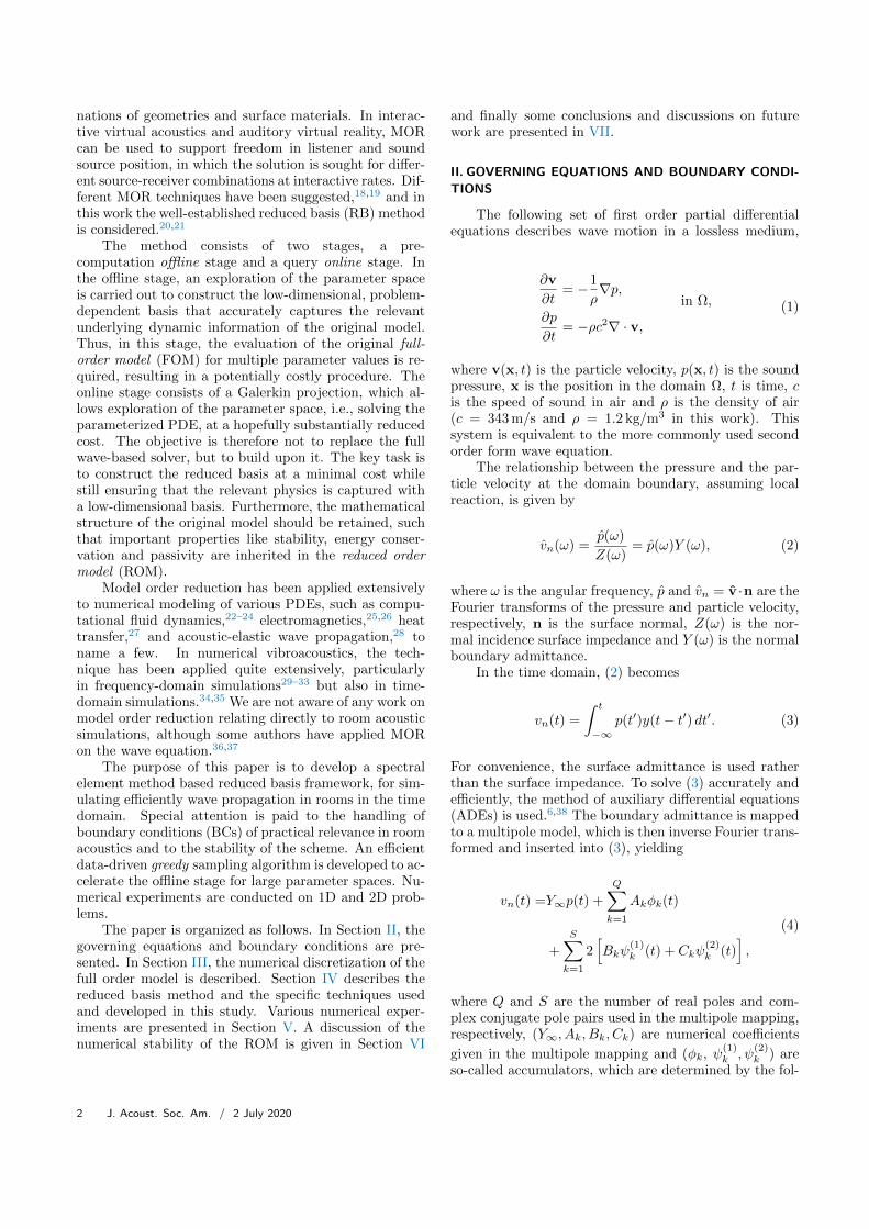
nations of geometries and surface materials. In interac-tive virtual acoustics and auditory virtual reality, MORcan be used to support freedom in listener and soundsource position, in which the solution is sought for differ-ent source-receiver combinations at interactive rates. Dif-ferent MOR techniques have been suggested,18,19 and inthis work the well-established reduced basis (RB) methodis considered.20,21
The method consists of two stages, a pre-computation offline stage and a query online stage. Inthe offline stage, an exploration of the parameter spaceis carried out to construct the low-dimensional, problem-dependent basis that accurately captures the relevantunderlying dynamic information of the original model.Thus, in this stage, the evaluation of the original full-order model (FOM) for multiple parameter values is re-quired, resulting in a potentially costly procedure. Theonline stage consists of a Galerkin projection, which al-lows exploration of the parameter space, i.e., solving theparameterized PDE, at a hopefully substantially reducedcost. The objective is therefore not to replace the fullwave-based solver, but to build upon it. The key task isto construct the reduced basis at a minimal cost whilestill ensuring that the relevant physics is captured witha low-dimensional basis. Furthermore, the mathematicalstructure of the original model should be retained, suchthat important properties like stability, energy conser-vation and passivity are inherited in the reduced ordermodel (ROM).
Model order reduction has been applied extensivelyto numerical modeling of various PDEs, such as compu-tational fluid dynamics,22–24 electromagnetics,25,26 heattransfer,27 and acoustic-elastic wave propagation,28 toname a few. In numerical vibroacoustics, the tech-nique has been applied quite extensively, particularlyin frequency-domain simulations29–33 but also in time-domain simulations.34,35 We are not aware of any work onmodel order reduction relating directly to room acousticsimulations, although some authors have applied MORon the wave equation.36,37
The purpose of this paper is to develop a spectralelement method based reduced basis framework, for sim-ulating efficiently wave propagation in rooms in the timedomain. Special attention is paid to the handling ofboundary conditions (BCs) of practical relevance in roomacoustics and to the stability of the scheme. An efficientdata-driven greedy sampling algorithm is developed to ac-celerate the offline stage for large parameter spaces. Nu-merical experiments are conducted on 1D and 2D prob-lems.
The paper is organized as follows. In Section II, thegoverning equations and boundary conditions are pre-sented. In Section III, the numerical discretization of thefull order model is described. Section IV describes thereduced basis method and the specific techniques usedand developed in this study. Various numerical exper-iments are presented in Section V. A discussion of thenumerical stability of the ROM is given in Section VI
and finally some conclusions and discussions on futurework are presented in VII.
II. GOVERNING EQUATIONS AND BOUNDARY CONDI-
TIONS
The following set of first order partial differentialequations describes wave motion in a lossless medium,
∂v
∂t= −1
ρ∇p,
in Ω,∂p
∂t= −ρc2∇ · v,
(1)
where v(x, t) is the particle velocity, p(x, t) is the soundpressure, x is the position in the domain Ω, t is time, cis the speed of sound in air and ρ is the density of air(c = 343 m/s and ρ = 1.2 kg/m3 in this work). Thissystem is equivalent to the more commonly used secondorder form wave equation.
The relationship between the pressure and the par-ticle velocity at the domain boundary, assuming localreaction, is given by
vn(ω) =p(ω)
Z(ω)= p(ω)Y (ω), (2)
where ω is the angular frequency, p and vn = v ·n are theFourier transforms of the pressure and particle velocity,respectively, n is the surface normal, Z(ω) is the nor-mal incidence surface impedance and Y (ω) is the normalboundary admittance.
In the time domain, (2) becomes
vn(t) =
∫ t
−∞p(t′)y(t− t′) dt′. (3)
For convenience, the surface admittance is used ratherthan the surface impedance. To solve (3) accurately andefficiently, the method of auxiliary differential equations(ADEs) is used.6,38 The boundary admittance is mappedto a multipole model, which is then inverse Fourier trans-formed and inserted into (3), yielding
vn(t) =Y∞p(t) +
Q∑
k=1
Akφk(t)
+S∑
k=1
2[Bkψ
(1)k (t) + Ckψ
(2)k (t)
],
(4)
where Q and S are the number of real poles and com-plex conjugate pole pairs used in the multipole mapping,respectively, (Y∞, Ak, Bk, Ck) are numerical coefficients
given in the multipole mapping and (φk, ψ(1)k , ψ
(2)k ) are
so-called accumulators, which are determined by the fol-
2 J. Acoust. Soc. Am. / 2 July 2020

lowing set of ordinary differential equations (ODEs)
dφkdt
+ λkφk(t) = p(t),
dψ(1)k
dt+ αkψ
(1)k (t) + βkψ
(2)k (t) = p(t),
dψ(2)k
dt+ αkψ
(2)k (t)− βkψ(1)
k (t) = 0.
(5)
This must be solved at the boundary at every timestep of the simulation. (λk, αk, βk) are numerical co-efficients from the multipole mapping. By choosing[Y∞, Ak, Bk, Ck] ∈ R and [λk, αk] ∈ R+, the admittancemodel is causal and real.
III. THE FULL ORDER MODEL
In this work, the numerical full order model of thegoverning equations, sometimes referred to as the “truth”solver or the “high-fidelity” solver in RB literature, isobtained by discretizing the spatial derivatives in (1) us-ing a spectral element method (SEM) and the tempo-ral derivatives using a fourth-order explicit Runge-Kuttamethod. The spectral element method is a nodal vari-ant of the finite element method that combines the at-tractive features of high-order accuracy and geometricflexibility39. Note, however, that any numerical dis-cretization approach for the FOM could be used. TheFOM solver is only briefly summarized here, a detaileddescription of the solver can be found in Ref.6.
The weak formulation of the governing equations,takes the following form
∫
Ω
vtφ dΩ = −1
ρ
∫
Ω
∇p φ dΩ,
∫
Ω
ptφ dΩ = −ρc2[∫
Γ
φn · v dΓ−∫
Ω
v · ∇φ dΩ
],
(6)
where Γ denotes the boundary of Ω and φ are globallycontinuous, piecewise test functions. The domain is di-vided into a set of non-overlapping elements Ωk, k =1, . . . , Nel and a set of nodes is mapped into each element,making up a total of Nfb degrees of freedom (DOFs) onthe mesh. The solution of the unknown variables v and pis represented as a series expansion of global basis func-tions N , defined by patching together local polynomialbasis functions, in this study taken to be Lagrange poly-nomials. By choosing the test functions to be equal tothe basis functions, i.e., defining a Galerkin scheme, thesemi-discrete system in 2D reads
Mut = −1
ρSkxp, Mvt = −1
ρSky p,
Mpt = ρc2(STx u+ STy v − vnB
),
(7)
where (u, v) are the (x, y) components of the particle ve-locity, respectively, M is the mass matrix, S is the stiff-ness matrix and B is a matrix responsible for surface
integration at the boundary. They are given by
Mij =
∫
Ω
NjNi dΩ ∈ RNfb×Nfb
(Sm)ij =
∫
Ω
∂Nj∂xm
Ni dΩ ∈ RNfb×Nfb ,
Bij =
∫
Γ
NjNi dΓ, ∈ RNfb×Nfb
(8)
where m is the mth Cartesian coordinate.The global matrix operators, which are sparse, are
determined by iterating over the elements and summingthe local matrix operators while relying on the propertyof domain decomposition. The semi-discrete system isthen integrated in time using the explicit Runge-Kuttatime stepping method.
IV. THE REDUCED BASIS METHOD
This section describes how the reduced basis methodcan be used to construct new, problem dependent spatialdiscretization operators of size Nrb, where Nrb Nfb.
A central concept in model order reduction is thesolution manifold
Mfb = qfb(µ)|µ ∈ P ⊂ Vfb, (9)
which is the set of all high-fidelity solutions qfb(x, t) =[u, v, p]T to the parametrized problem under variationof the parameter µ belonging to the parameter spaceP. Vfb is the discete finite element approximation space.Note that when reducing time-dependent partial differ-ential equations, the standard approach is to take timeas being one of the parameters in the parameter space.The objective of a reduced order model is to approxi-mate any member of this solution manifold with a smallnumber of basis functions. Thus, a key assumption inprojection-based model order reduction is thatMfb is oflow dimension, such that the span of a low number of ap-propriately chosen basis functions φiNrb
i=1 represents the
solution manifold within a small error. The set φiNrbi=1
is called the reduced basis and Vrb = spanφ1, . . . , φNrb
is the reduced basis space. The reduced basis solutionto the PDE is then expressed as a linear combinationof the reduced basis functions φi(x) and time-dependentcoefficients ai(t), as follows
qfb(x, t) ≈ qrb(x, t) =
Nrb∑
i=1
φi(x)ai(t), (10)
or, written in matrix form,
qrb(x, t) = Φa, (11)
where Φ ∈ RNfb×Nrb is a matrix containing the reducedbasis vectors as its column and a ∈ RNrb is a vectorcontaining the coefficients.
A measure of how well Mfb can be approximatedwith a smaller subspace Vrb is given by the Kolmogorov
J. Acoust. Soc. Am. / 2 July 2020 3

N -width of Mfb, defined as
dN (Mfb) = infVrb
supqfb∈Mfb
infqrb∈Vrb
||qfb − qrb||V. (12)
The N -width is highly dependent on the PDE beingsolved and on the initial and boundary conditions aswell. For some PDEs, the N -width decays exponentiallyfast dN (Mfb) = O(eβNrb), making them highly suited forprojection-based model reduction. Hyperbolic problemsare known to be less well suited for model order reduc-tion than various elliptic or parabolic problems, due toa slower decay of dN (Mfb).40,41 However, the decay rateis highly case dependent, and many examples exist inthe literature where MOR has been applied successfullyon hyperbolic problems.22–26,28–37 Due to the problem-dependency of the N -width decay rate, it is of great inter-est to investigate how suitable MOR is for room acousticsproblems.
A. The offline stage – sampling and basis generation
As mentioned in the introduction, MOR using theRB method is carried out in two stages, the offline stageand the online stage. During the offline stage, the so-lution manifold is empirically explored and the reducedbasis is constructed. A key question is how to constructthe reduced basis optimally, such that the relevant un-derlying physics are captured in the ROM, while the costof the offline stage is minimized. Different methods havebeen proposed in the literature. In this work, two ap-proaches are considered, the proper orthogonal decom-position (POD) method, for the case when time is takento be the only varying parameter of the system, and anovel data-driven greedy-POD basis generation method,for the case when the parameter space is extended to in-clude boundary condition parameters as well. These twoapproaches are described here below.
1. Proper Orthogonal Decomposition
The POD is a mathematical technique used for datacompression and low-dimensional approximation. It isclosely related to principal component analysis. Thetechnique provides an optimally ordered, orthogonal ba-sis in the least-squares sense. Reduced order models arethen obtained by truncating this optimal basis, retain-ing only the essential information that ensures the pre-defined desired accuracy is obtained.
When using POD for basis generation, the param-eter space is discretized Ph ⊂ P, often using a uniformdistribution. An appropriate discretization density of theparameter space must be selected such that the dynam-ics of the solutions is accurately represented in the snap-shots. Given that the discretization of Ph is fine enough,Mfb(Ph) will be a good representation of Mfb. Samplesof the high-fidelity solutions, called snapshots, for the pa-rameter values in Ph are collected. Note that when usingPOD for compressing time-dependent problems, the timetrajectory must be discretized very finely to preserve sta-bility of the high-fidelity simulator. However, snapshots
do not necessarily have to be stored at every time step ofthe high fidelity solution for the basis generation process.
The snapshots are gathered into a snapshot matrix
S = [qfb(x, t0), qfb(x, t1), . . . , qfb(x, tK)] ∈ RNfb×K (13)
where K is the total number of time steps and qfb(x, t0) isthe inital condition. By design, the POD basis functionsare orthogonal to each other, 〈φi, φj〉L2(Ω) = δij , whereδij is the Kronecker delta function and 〈·, ·〉L2(Ω) denotesthe L2 inner product over the domain Ω. Using the L2
norm is preferred for discrete schemes.42 Thus, the PODbasis Φ is optimal when the difference between the snap-shots and the projection of the snapsnots onto the basisfunctions is minimal for a given norm. The minimizationproblem is, therefore, given by
Φ = minφiNrb
i=1
K∑
j=1
∣∣∣∣∣
∣∣∣∣∣qfb(x, tj)−Nrb∑
i=1
〈qfb(x, tj), φi(x)〉L2φi(x)
∣∣∣∣∣
∣∣∣∣∣
2
L2
.
(14)The minimization problem can be solved using singularvalue decomposition (SVD) on the snapshot matrix S =UΣVT , where Φ = [U1, . . . , UNrb
], where Ui is the ithleft singular vector. The singular values Σii, provide ameasure of the error of the reduced basis in the energysense and are bounded from above by the KolmogorovN -width.43
An equivalent but computationally leaner method isto solve an eigenvalue problem44,45
CQ = Qλλλ, (15)
where C ∈ RK×K is a correlation matrix given by Cij =〈qfb(x, ti), qfb(x, tj)〉L2(Ω), Q is a square matrix whosecolumns are the eigenvectors and λλλ is a diagonal matrixcontaining the eigenvalues λii. The POD basis functionsare then given by
φi =1√λii
SQi. (16)
2. Data-driven greedy-POD basis generation
Obtaining an optimal basis using POD for multi-dimensional parameter spaces can result in a computa-tionally very expensive offline stage. This is because sev-eral sampling points may contain only redundant infor-mation that does not enrich the reduced basis. In otherwords, the high fidelity solution is evaluated K timesto generate a reduced basis of size Nrb, and generallyK Nrb. This motivates the use of iterative basis gen-eration methods, called greedy sampling. Here, the pa-rameter space exploration is driven by a computationallycheap error estimator η(µ), where
||qfb(µ)− qrb(µ)|| ≤ η(µ). (17)
The error estimator dictates where to sample next inthe iterative process, and the basis is enriched with onenew basis function for each iteration, until a predefined
4 J. Acoust. Soc. Am. / 2 July 2020

threshold in the error estimator is reached. Thus, togenerate a reduced basis of size Nrb, the greedy samplingalgorithm evaluates the high-fidelity solution Nrb times.This way, the exploration of redundant sampling pointsis avoided. When reducing time dependent problems,it is appropriate to combine greedy and POD methods,where the POD is used for the time trajectory (whichmust anyway be discretized uniformly in the FOM) and agreedy algorithm is used for other parameters, e.g, relat-ing to the boundary conditions or source positions. Thisis called greedy-POD sampling. Thus in every iterationof the greedy algorithm, a POD reduction is performedon the time trajectory.
Clearly, a key component of the greedy sampling al-gorithm is the error estimator. The purpose of the esti-mator is to cheaply evaluate for which parameter value µthe difference between the ROM and FOM is maximized.This can then be used to guide the sampling algorithm tosample at the parameter values that contribute the great-est amount of new information to the reduced basis, i.e.,
µn+1 = arg maxµ∈P
η(µ). (18)
While considerable work has been carried out for de-veloping cheap error estimators for non-time-dependentproblems,20 it is difficult to get a cheap and sharp esti-mation of the error for time dependent problems. This is,e.g., a long-standing problem in adaptive ODE solvers.The challenge is that, generally, the error cannot be ac-curately estimated unless the FOM is solved for all timesteps, thereby defeating the purpose of greedy sampling.
In this work, we propose to use a data-driven greedy-POD sampling strategy, where the greedy parameterspace exploration is driven by a Gaussian process re-gression (GPR) model. This data-driven paradigm issometimes called active learning.46–49 The key idea be-hind active learning is that a machine learning algorithmcan achieve greater accuracy with fewer data points ifit is allowed to select the sampling points by studyingthe data from which it learns. Since the GPR is fast toevaluate, (18) can be computed quickly over a finely dis-cretized parameter space. An initial quasi-Monte Carlodistribution of L parameter sampling points across theparameter space is defined, e.g., a Sobol sequence, andthe error of the ROM η(µ) for these initial values is com-puted. A Gaussian regression model is then fitted to thiserror data, and the variance of the Gaussian model isused as the error estimator, i.e., the algorithm samplesnext where the variance is maximized. This ensures thatthe most informative sampling points are explored andused to construct the basis, and that the algorithm onlysamples as is needed. Once the variance has reached apredefined threshold ε, the algorithm terminates. Thealgorithm is summarized in Algorithm 1.
B. The online stage
The online stage consists of a Galerkin projectiononto the span of the reduced basis, where the parameter
Algorithm 1: The data-driven Greedy-PODalgorithm for efficient basis generation
Input: Initial Sobol sequence parameter set
Γ = µ1, . . . , µL, variance trehshold ε,
number of POD basis functions to include for
time compression NPOD, number of total basis
functions to include Nrb.
Result: The reduced basis Φ
1 k = 1
2 for µi in Γ
3 Compute FOM time trajectory S∗ = qfb(µi)
4 POD on time trajectory S∗ = UΣVT
5 Truncate time trajectory Φ∗ = [U1, . . . , UNPOD ]
6 S← Φ∗
7 Compute ROM time trajectory qrb(µi)
8 η(k) = ||qfb(µi)− qrb(µi)||9 k = k+1
10 end
11 Fit GPR model to the error data η
12 Compute variance σ2 of GPR model
13 while maxσ2 > ε
14 µ = arg maxµ∈P σ2
15 Compute FOM time trajectory S∗ = qfb(µ)
16 POD on time trajectory S∗ = UΣVT
17 Truncate time trajectory Φ∗ = [U1, . . . , UNPOD ]
18 S← Φ∗
19 Compute ROM time trajectory qrb(µ)
20 η(k) = ||qfb(µ)− qrb(µ)||21 k = k+1
22 Re-fit GPR model to the error data η
23 Compute variance σ2 of GPR model
24 end
25 POD on snapshot matrix S = UΣVT
26 Truncate Φ = [U1, . . . , UNrb ]
space can be explored at a significantly reduced cost, as-suming that the solution manifold can be approximatedwith sufficient accuracy using Nrb basis functions, whereNrb Nfb. In general, for linear problems, the evalua-tion of the solution during the online stage is completelyindependent of the original high-fidelity problem, mean-ing that the cost is dictated by Nrb and not by Nfb dur-ing the online stage. However, as will be seen in SectionV A 2, when incorporating frequency dependent bound-ary conditions, it is difficult to make the online stagecompletely independent of Nfb, however, the computa-tional cost is still significantly reduced.
Assuming a semi-discrete FOM system on the form
qt = Lq, (19)
the semi-discrete ROM is obtained by inserting the re-duced basis assumption (10) into (19), which yields
(Φa)t = LΦa, (20)
i.e.at = ΦTLΦa, (21)
J. Acoust. Soc. Am. / 2 July 2020 5

due to the orthogonality of the reduced basis. The ROMspatial discretization operator ΦTLΦ ∈ RNrb×Nrb can becomputed prior to the online stage. In the online stagethe semi-discrete system in (21) is integrated in time us-ing standard time stepping methods, for any parametervalue µ. The initial condition q(x, 0) is also projected,i.e., a(0) = ΦT q(x, 0). Once the ROM has been solvedfor a, the output of interest is evaluated with q = Φa.
One critical issue which has not been discussed yet isthe numerical stability of the ROM. In general, a time-dependent ROM will not inherit the stability propertiesof the FOM, due to a loss of the structure of the spatialdiscretization operator when the model reduction is ap-plied. The issue of ROM stability is discussed further inSec. VI.
V. NUMERICAL EXPERIMENTS
A. POD-based MOR with time as the only parameter
In this section the reduced basis method is appliedon (1) where the only varying parameter of the system istime. First, the frequency independent BC case is consid-ered in Section V A 1 and then the frequency dependentBC case is considered in Section V A 2. Later, in SectionV B, the parameter space is extended to include bound-ary condition parameters as well, although, limited tofrequency independent BCs.
1. Frequency independent BCs
The FOM simulator is run to generate snapshotsof the problem solution for each of the field quantities(u, v, p), for K time steps. Due to the large amplitudedifference between the particle velocity and the pres-sure, separate reduced bases are constructed for eachfield quantity. Thus, separate snapshot matrices are con-structed from the FOM solution, i.e., Su,Sv,Sp, whichcontain the solution at all nodes across the time trajec-tory.
The reduced basis Φ is then constructed by perform-ing a SVD on the snapshot matrices, and then selectingthe Nrb leftmost singular vectors, e.g.,
Φp = [U1, . . . , UNrb], (22)
where Ui is the ith left singular vector of the snapshotmatrix Sp.
In the case of frequency independent BCs, the semi-discrete system in (7) becomes
Mut = −1
ρSkxp, Mvt = −1
ρSky p,
Mpt = ρc2(STx u+ STy v −
p
ZB),
(23)
which can be written as
ut = L1p,
vt = L2p,
pt = L3u+ L4v + L5p.
(24)
By inserting the reduced basis assumption (10) into (24),the ROM becomes
(au)t = ΦTuL1Φpap,
(av)t = ΦTv L2Φpap,
(ap)t = ΦTp L3Φuu+ ΦTp L4Φvv + ΦTp L5Φpap.
(25)
A 2 m × 2 m rectangular domain is tested. Thesurface impedance for all four bounding surfaces is takento be Z = 5, 000 Ns/m4, corresponding to a normal inci-dence absorption coefficient of α0 ≈ 0.28. The simulationis initiated with a Gaussian pulse pressure distribution,
p(x, 0) = exp
(− (x− xs)2 + (y − ys)2
σg
), (26)
with a spatial variance of σg = 0.3 m2. This yields abroadband initial pulse that has a −10 dB upper cutofffrequency of around 700 Hz. The pulse is centered at(xs, ys) = (0.7, 1.2). The domain is meshed with an un-structured mesh of triangular elements and N = 4 basisfunctions are used. The resolution of the mesh is chosensuch that there are approximately 7 points per wave-length (PPW) at 700 Hz. This yields a mesh that has 88elements and Nfb = 761 DOFs in total. The simulationtime is 50 ms.
Figure 1 shows the resulting singular values after per-forming the SVD on the snapshot matrices. The decay ofthe singular values indicates that a low-dimensional solu-tion manifold exists. The energy decay is very similar forthe three different field quantities. Table I lists the num-ber of basis functions needed to obtain specific normal-ized singular values E/E0. The table also lists the numer-ical error of the ROM, defined as ε = ||pFOM− pROM||∞.
FIG. 1. Singular value decay for the 2 m × 2 m test case with
frequency independent boundaries.
Figure 2 shows simulation results when using theFOM or the ROM for the different Nrb values in TableI. The figure shows the pressure response in an arbitrar-ily selected node on the mesh. For the E/E0 = 10−2
case (Nrb = 40), some clear deviations of the ROM fromthe FOM solution are observed, especially at later timevalues. However, already for the E/E0 = 10−3 case(Nrb = 72), an excellent agreement between the FOMand the ROM is observed, even though the reduced basisin this case is around 10 times smaller than the full basis.
6 J. Acoust. Soc. Am. / 2 July 2020

E/E0 Nrb ε
10−2 40 6.9 · 10−2
10−3 72 8.9 · 10−3
10−4 159 8.9 · 10−4
TABLE I. Number of basis functions Nrb needed to obtain
a particular normalized singular value E/E0 and the ROM
error ε. The FOM size is Nfb = 761.
FIG. 2. Simulated pressure using the FOM and the ROM
using different levels of basis compression, for the frequency
independent BCs.
Since the reduction ability is highly influenced by thesingular value decay (which is related to the KolmogorovN -width), it is of interest to investigate how the singularvalue decay changes as the simulation conditions change,e.g., the domain size, the integration time or the bound-ary conditions. Thus, a study is carried out, where thesingular value decay is analyzed for different scenarios.Two rectangular spatial domains are considered, D1 andD2, where D1 is 2 m × 2 m and D2 is 4 m × 4 m. N = 4basis functions are used and both domains are meshedwith unstructured meshes of triangular elements with aresolution of roughly 7 PPW at 700 Hz. This means thatNfb = 761 for D1 and Nfb = 3141 for D2. Two bound-ary conditions are considered, Z1 = 5, 000 Ns/m4 andZ2 = 20, 000 Ns/m4 (α0 ≈ 0.08), and two simulation fi-nal times tf as well. In all cases the same initial conditionas described above is used.
Table II shows the amount of basis functions neededto obtain a normalized singular value of E/E0 = 10−3.It is clear that in all cases, a low-dimensional subspaceexists and the problem can be solved with the prescribedaccuracy in the singular values, using a significantly re-duced basis. Particularly for the larger domain, a signifi-cant reduction potential is observed. This indicates thatthe dimension of the solution manifoldMfb grows slowerthan the number of DOFs. The boundary conditions andthe integration time have less of an influence.
Table III shows the same results but for the casewhen the singular value threshold is decreased to E/E0 =10−5. As expected, reaching a higher level of accuracy re-quires more basis functions. Furthermore, it is observed
D1 D2
tf Z1 Z2 Z1 Z2
0.05 72 (9.5%) 67 (8.8%) 99 (3.2%) 101 (3.2%)
0.2 86 (11.3%) 86 (11.3%) 235 (7.5%) 257 (8.2%)
TABLE II. Number of basis functions needed to obtain a nor-
malized level of 10−3 in the singular value decay. The value
in the parenthesis indicates the percentage ratio Nrb/Nfb.
that the integration time and the boundary conditionshave a bigger influence on the reduction potential. Thelonger we wish to simulate and the less absorbing theboundary conditions are, the more difficult it is to re-duce the system.
D1 D2
tf Z1 Z2 Z1 Z2
0.05 230 (30.2%) 238 (31.3%) 254 (8.1%) 268 (8.5%)
0.2 302 (39.7%) 506 (66.5%) 839 (26.7%) 894 (28.5%)
TABLE III. Number of basis functions needed to obtain a
normalized level of 10−5 in the singular value decay. The value
in the parenthesis indicates the percentage ratio Nrb/Nfb.
2. Frequency dependent BCs
In the FOM for the frequency independent BC case,the boundary condition was incorporated into the L5
spatial discretization operator. This allows us to usestandard reduced basis techniques to generate the ROM,where the BC was incorporated into a reduced operator.The frequency dependent case is not as straightforward,because in order to solve the ADEs in (5), the pressureat the boundary must be known, also in the ROM.
The semi-discrete system in (7) is rewritten as
ut = L1p,
vt = L2p,
pt = L3u+ L4v + L5vn,
(27)
where vn is given by (4) at the boundary. This FOM issolved to generate the snapshots. In addition to generat-ing snapshot matrices for the field quantities (u, v, p), asnapshot matrix is also generated for the normal velocityvn at the boundary, yielding a total of four snapshot ma-trices. An SVD is applied to the snapshot matrices andthe reduced bases are constructed by selecting the firstNrb singular vectors.
J. Acoust. Soc. Am. / 2 July 2020 7

Inserting the reduced basis assumption (10) into (27)yields the ROM,
(au)t = ΦTuL1Φpap,
(av)t = ΦTv L2Φpap,
(ap)t = ΦTp L3Φuu+ ΦTp L4Φvv + ΦTp L5Φvnavn .
(28)
To compute the boundary contribution avn in the ROM,the reduced solution ap is used to retrieve p at the bound-ary using p = Φpap. This is then used when solvingthe ADEs in (5) to compute vn, which is then projectedback to avn = ΦTvnvn. This implies that the online stageof the ROM with frequency dependent BCs is not fullyde-coupled from Nfb. Nevertheless, this additional pro-jection of the boundary condition has limited influence onthe efficiency of the ROM in the numerical experiments.
A test case is set up where a 2 m × 2m rectangulardomain is used. The same mesh resolution and the samesource conditions as described in Sec. V A 1 are used.First, a modestly absorbing boundary condition is ap-plied to all bounding surfaces, modeled as a dmat = 0.05m thick porous material mounted on a rigid backing andhaving flow resistivity σmat = 10, 000 Ns/m4. The char-acteristic impedance and wave propagation constant ofthe porous material are obtained by using Miki’s model,50
and the surface impedance is computed using a transfermatrix method.51 In the multipole mapping, the mate-rial is mapped using vector fitting,52 with 4 poles. Asimulation time of 0.1 s is used.
Figure 3 shows the singular value decay. Note thatfewer nodes exist at the domain boundary than in thewhole domain, which explains the sharp drop in the sin-gular values for the boundary velocity vn. Figure 4 showsthe FOM and ROM simulation results for an arbitrarynode on the mesh. The ROM is shown for Nrb = 24basis functions, corresponding to a normalized singularvalue decay level of E/E0 = 10−2, and for Nrb = 82 basisfunctions, corresponding to a normalized singular valuedecay level of E/E0 = 10−4. For the former case, someclear differences between the FOM and the ROM are ob-served. However, for the latter case, the ROM capturesthe FOM with high precision.
FIG. 3. Singular value decay for the 2 m × 2 m test case
with frequency dependent boundaries. The boundary is a
porous material of thickness d = 0.05 m and has flow resis-
tivity σmat = 10, 000 Ns/m4.
FIG. 4. Simulated pressure using the FOM and the ROM
using different levels of basis compression, for the frequency
dependent BCs with d = 0.05 m and σmat = 10, 000 Ns/m4.
Figures 5 and 6 show analogous results for a differentboundary condition, where the porous material thicknesshas been increased to dmat = 0.2 m, to make the bound-ary more absorbing. A similar behavior is observed here,and the ROM is capable of accurately capturing the FOMwith a low-dimensional basis.
Note that the reduced basis method can also be ap-plied on the ADE system in (5). Our numerical exper-iments indicate that this does not yield noticeable im-provements in computational efficiency. This can be ex-plained by the fact that the cost of solving the ADEs isalready very small compared to solving the main semi-discrete system.
FIG. 5. Singular value decay for the 2 m × 2 m test case
with frequency dependent boundaries. The boundary is a
porous material of thickness d = 0.2 m and has flow resistivity
σmat = 10, 000 Ns/m4.
B. Greedy-POD MOR with parameterized boundary condi-
tions
In the ROMs presented in the previous section, theonly varying parameter of the parameter space was takento be time. In principle, these ROMs could be used forcomputing the solution for any t in the range [0, tf ], e.g.,at values between sampling points, at a reduced cost,compared to solving the FOM. However, this is hardly ofpractical relevance, since it is anyway needed to samplethe FOM very finely in time for determining the ROM,due to stability conditions in the FOM. What is of prac-tical relevance is when the parameter space is extended
8 J. Acoust. Soc. Am. / 2 July 2020

FIG. 6. Simulated pressure using the FOM and the ROM
using different levels of basis compression, for the frequency
dependent BCs with d = 0.2 m and σmat = 10, 000 Ns/m4.
to include other parameters too, such as the boundaryconditions or the source position. This would allow,e.g., rapid virtual prototyping or simulations of interac-tive scenes at fast rates, as discussed in the introduction.For this purpose, the greedy-POD algorithm developedin Sec. IV A 2 can be used.
A test case is set up, where a 3 m × 3 m rectan-gular domain is used. Otherwise, the same simulationconfigurations as in Section V A 1 are used, i.e., a basisfunction order of N = 4, a mesh resolution of 7 PPW at700 Hz, a source position (xs, ys) = (0.7, 1.2), a sourcewidth of σg = 0.3 m2 and a final time of tf = 0.05 s. TheFOM size is Nfb = 1775 DOFs. The parameter space isnow taken to be both time and the frequency indepen-dent boundary surface impedance Z. The impedance isallowed to take any value in the range Z ∈ [500, 10000]Ns/m4 (α0 ∈ [0.15, 0.99]). An initial Sobol sequence ofL = 4 samples across the impedance parameter spaceis used for Γ. The greedy-POD algorithm is run witha variance threshold of ε = 3 · 10−5, NPOD = 100 andNrb = 360.
The greedy algorithm converges after 15 iterations.Figure 7 shows the GPR model at different iterations.After the initial fit, the variance σ2 is high. In thenext iteration, the algorithm samples in the parameterspace where the variance is highest. As more observa-tions are added to the data, the variance decreases, untilthe threshold ε is reached.
Figure 8 shows the singular value decay for the fi-nal snapshot matrix S. In order to reach a level ofE/E0 = 10−3, around Nrb = 360 basis functions areused, i.e., around 20% of the original problem size Nfb.Figure 9 shows a comparison of FOM and ROM resultsfor boundary surface impedance values that do not be-long to the training set. The figure shows the pressurein an arbitrarily selected node on the mesh. The ROMprovides a good approximation to the full model.
VI. IN PURSUIT OF STABILITY
The issue of stability is of crucial importance in time-domain model order reduction. While stability has beenpreserved in all numerical experiments so far, the stabil-ity properties of the FOM are in general not inherited
a) Initial GPR model.
b) GPR model after 9 iterations.
c) GPR model after the last iteration.
FIG. 7. ROM error across the parameter space, along with
the fitted GPR model. The shaded gray area shows the 95%
confidence interval of the GPR model, which is proportional
to the variance σ2. After the initial GPR is fitted, the al-
gorithm samples next at Z ≈ 10, 000 Ns/m4 (a). After 9
iterations the algorithm samples next at Z ≈ 6, 000 Ns/m4
(b). The error is normalized to the maximum error level.
by the ROM, because the structure of the spatial dis-cretization operators is lost when the basis reduction isperformed using standard MOR techniques such as thePOD. Indeed, for long-time numerical simulations, in-stability in the ROM occurs regularly. Different meth-ods have been proposed to address the stability of time-dependent ROMs. The balanced truncation method en-sures stability, but scales poorly with problem size, yield-ing an unpractical method.53 Optimization approacheshave also been suggested, where the projection basis ismodified to preserve stability.54,55 The drawback of theseapproaches is that a trade-off between accuracy and sta-bility occurs and, moreover, feasible solutions cannot beguaranteed in a finite number of iterations, restrictingtheir use in practical problems. In the domain of nu-merical vibroacoustics, van de Walle et al.34 proposed
J. Acoust. Soc. Am. / 2 July 2020 9

FIG. 8. Singular value decay for the total snapshot matrix S
for the greedy-POD test case.
a) Z = 1800 Ns/m4.
b) Z = 8500 Ns/m4.
FIG. 9. ROM compared to the FOM for boundary impedance
values chosen to be different from the training parameters,
when using the greedy-POD method.
a structure-preserving ROM formulation of the secondorder vibroacoustics governing equations that preservesstability. However, this approach relies on a problem-specific formulation of the fluid-structure vibroacousticsgoverning equations. Moreover, this approach is re-stricted to frequency independent BCs and a parameterspace that consists only of time.
A. Hamiltonian systems and symplectic model reduction
A way to ensure the stability of a ROM is to refor-mulate the problem as a Hamiltonian system and usesymplectic model reduction techniques. A Hamiltoniansystem is a dynamical system, which is completely de-scribed by the scalar function H(q,p, t), which is calledthe Hamiltonian. The variable q is generally called themomentum and p is called the potential. The evolution
equations are then given by
qt = ∇pH(q,p),
pt = −∇qH(q,p),(29)
which can equivalently be written as
zt = J2Nfb∇zH(z), (30)
where z = (qT ,pT )T and
J2Nfb=
[0Nfb
INfb
INfb0Nfb
]. (31)
An important feature of Hamiltonian systems is that theyhave a symplectic structure, meaning that the Hamilto-nian is conserved along the integral curves of a symplecticmanifold. This gives rise to an opportunity for using sym-plectic model reduction techniques, where the symplecticstructure of the FOM is preserved in the ROM. This, inturn, ensures that the stability properties of the FOMare inherited by the ROM. Suppose A ∈ R2Nfb×2Nrb is asymplectic low-dimensional basis that approximates thesolution manifold MH of (30). Applying the reducedbasis assumption (10) yields
z ≈ Aa. (32)
Inserting this into (30) yields
(Aa)t = J2Nfb∇zH(Aa). (33)
Multiplying both sides of (33) with the symplectic inverseof A, denoted A+, and applying the chain rule, gives
a = A+J2Nfb(A+)T∇aH(Aa). (34)
Since A is a symplectic basis, (A+)T is a symplectic ma-trix, i.e., A+J2Nfb
(A+)T = J2Nrb. A reduced Hamilto-
nian H(a) = H(Aa) is defined and the reduced Hamilto-nian system becomes
at = J2Nrb∇aH(a). (35)
The reduced system in (35) is of the same form as the fullorder system in (30), meaning that the symplectic struc-ture is conserved and hence the numerical stability ofthe reduced system is guaranteed. The reader is referredto Ref.37 and the references therein for a more in-depthdescription and detailed mathematical proofs relating tomodel reduction of Hamiltonian systems.
When symplectic systems, such as Hamiltonian sys-tems (either in their FOM or ROM formulations), areintegrated in time, standard time-stepping schemes, e.g.,Runge-Kutta methods, cannot be applied because theygenerally do not preserve the Hamiltonian.56 Insteadsymplectic time integrators must be used, which preservethe system structure, energy and stability. The Stormer-Verlet scheme is an example of a second order symplectic
10 J. Acoust. Soc. Am. / 2 July 2020

time stepping scheme, and is used in this work. It reads
qn+1/2 = qn +∆t
2∇pH(qn+1/2,pn),
pn+1 = pn −∆t
2(∇qH(qn+1/2,pn)
+∇qH(qn+1/2,pn+1/2)),
qn+1 = qn+1/2 +∆t
2∇pH(qn+1/2,pn+1/2),
(36)
For general Hamiltonian systems, the Stormer–Verletscheme is implicit. However, for separable Hamiltoni-ans, i.e., H(q,p) = K(p) + U(q), the scheme becomesexplicit.
A symplectic projection is similar to the Galerkinprojection, and both construct reduced systems in a low-dimensional subspace. However, the symplectic projec-tion yields a reduced symplectic system on the form(35), while the Galerkin projection generally destroysthe symplectic structure. Different symplectic model re-duction techniques exist. In this work, we employ theproper symplectic decomposition (PSD) method, in par-ticular the cotangent lift approach, which is an SVD-based PSD method.57 When using PSD, a similar mini-mization problem is solved as in the POD method. How-ever, the symplectic bases are generally not orthogonal,and therefore not norm bounded, making the minimiza-tion problem harder to solve than in the POD case.58
Suppose that A is on the form
A =
[ΦH 0
0 ΦH
], (37)
where ΦH ∈ RNfb×Nrb is an orthonormal matrix. Clearly,A is a symplectic matrix, i.e., AT J2Nfb
A = J2Nrb. The
structure of A implies that ΦH should cover both themomentum and potential spaces. Therefore, a combinedsnapshot matrix must be defined
Sc = [q(x, t0), . . .q(x, tK),p(x, t0) . . .p(x, tK)], (38)
and then ΦH is given by selecting the Nrb leftmost sin-gular vectors after performing an SVD on the combinedsnapshot matrix, i.e., ΦH = [U1, . . . UNrb
]. Of all baseson the form (37), the cotangent lift method minimizesthe projection error.57
Thus, to summarize, a stable ROM can be obtainedby reformulating the problem as a Hamiltonian system,using symplectic time integration and applying a PSDprojection method, such as the cotangent lift method,where a combined snapshot matrix must be constructedin a specific way.
B. 1D numerical example with rigid BCs
Note that the first order form of the wave equationintroduced in (1) is the Hamiltonian form of the waveequation, which means that no further reformulation ofthe governing equations is needed. The Stormer-Verlet
scheme for the 1D wave equation reads
un+1/2 = un +∆t
2L1pn,
pn+1 = pn + ∆tL2un,
un+1 = un+1/2 +∆t
2L1pn+1.
(39)
where L1 =M−1((−1/ρ)Sx) and L2 =M−1(ρc2STx ) arethe spatial discretization operators. The snapshot matrixis structured as
Sc = [u(x, t0), . . . , u(x, tK), p(x, t0), . . . , p(x, tK)] (40)
A 1D domain in the range of x ∈ [−1, 1] is constructedand meshed using a uniform mesh. A Gaussian pulsepressure initial condition is used with σg = 0.2 m2, whichhas a −10 dB upper cutoff frequency of around 1050 Hz.N = 4 basis functions are used and the spatial resolutionis around 6.5 PPW at 1050 Hz. The FOM is solved and aROM is created using both standard RB techniques, i.e.,the Galerkin projection, and the symplectic approach.Figure 10 shows the resulting pressure in an arbitrarilyselected node on the mesh. The standard ROM approachresults in a numerically unstable scheme, whereas thesymplectic approach preserves stability.
VII. CONCLUSION AND FUTURE WORK
Model order reduction, using the reduced basismethod, has been applied to the wave equation problemfor 1D and 2D problems. It was shown that there appearsto be a potential for using these techniques for accel-erating wave-based room acoustics simulations in caseswhere the solution is sought for a large number of pa-rameters, e.g., in iterative design or in dynamic auditoryvirtual reality setups. A way to incorporate frequencydependent boundaries into the reduced model was pro-posed and various numerical experiments showed thatthe reduced model gives a good approximation of the fullmodel.
A novel data-driven greedy-POD sampling algorithmwas proposed, which can potentially accelerate the offlinepre-computation stage, as compared to using standardproper orthogonal decomposition methods when explor-ing the parameter space.
Furthermore, the stability of the reduced numeri-cal scheme is studied and an approach using symplecticmodel reduction is suggested as a way of ensuring sta-bility of the reduced model. A 1D numerical experimentwith rigid BCs illustrates the stability of the symplecticapproach.
While these preliminary results are promising, fur-ther research on the topic is needed. This includes:
• Extending the Hamiltonian model to include ab-sorbing boundary conditions, in particular fre-quency dependent boundary conditions, is neces-sary for the reduced model to be useful in practicalscenarios. Standard Hamiltonian systems rely on
J. Acoust. Soc. Am. / 2 July 2020 11

FIG. 10. Comparison of ROM results when using either the standard Galerkin approach or the symplectic approach, for a 1D
test case with rigid BCs.
energy conservation, making the extension to thedissipative case not straightforward. However, re-cent work by Afkham et al.59 proposed a way to re-formulate the Hamiltonian system such that energydissipation is stored in hidden strings, and appliedit to the 1D dissipative wave equation with good re-sults. However, it remains to be seen whether thisapproach can be extended effectively to include fre-quency dependent boundary conditions.
• Further analysis of the greedy-POD algorithm isneeded to see how much it can reduce the cost of theoffline stage, as compared to using standard uni-form sampling techniques. Extending the greedyalgorithm to the Hamiltonian system is also of in-terest and perhaps this allows for the use of othererror estimators, see, e.g., Ref.37
• Penalty techniques are an interesting approach forenforcing boundary conditions, and could be a wayto enforce the frequency dependent BCs in theROM which circumvents the need to project be-tween the reduced solution and the full solution inevery time step, see, e.g., Ref.60
• It is of interest to investigate how much accuracyin the ROM is needed, e.g., what level of singularvalue energy, for the ROM results to be perceptu-ally indistinguishable from the FOM.
• Since the benefits of using reduced basis methodsare very problem dependent, a thorough analysis ofthe reduction potential for realistic room scenariosis in order.
ACKNOWLEDGMENTS
This research has been partially funded by the Inno-vation foundation and the Realdania foundation in Den-mark.
REFERENCES
1L. Savioja and U. P. Svensson. Overview of geometrical roomacoustic modeling techniques. J. Acoust. Soc. Am., 138(2):708–730, 2015.
2D. Botteldooren. Finite-difference time-domain simulation oflow-frequency room acoustic problems. J. Acoust. Soc. Am.,98(6):3302–3308, 1995.
3S. Bilbao. Modeling of complex geometries and boundary condi-tions in finite difference/finite volume time domain room acous-tics simulation. IEEE Trans. Audio, Speech, Lang. Proc.,21(7):1524–1533, 2013.
4J. A. Hargreaves, L. R. Rendell, and Y. W. Lam. A framework forauralization of boundary element method simulations includingsource and receiver directivity. J.Acoust. Soc. Am., 145(4):2625–2637, 2019.
5A. Craggs. A finite element method for free vibration of airin ducts and rooms with absorbing walls. J. Sound Vib.,173(4):568–576, 1994.
6F. Pind, A. P. Engsig-Karup, C. H. Jeong, J. S. Hesthaven, M. S.Mejling, and J. Strømann Andersen. Time domain room acousticsimulations using the spectral element method. J. Acoust. Soc.Am., 145(6):3299–3310, 2019.
7H. Wang, I. Sihar, R. Pagan Munoz, and M. Hornikx. Roomacoustics modelling in the time-domain with the nodal discontin-uous Galerkin method. J. Acoust. Soc. Am., 145(4):2650–2663,2019.
8B. Hamilton and S. Bilbao. FDTD methods for 3-D room acous-tics simulation with high-order accuracy in space and time. IEEETrans. Audio, Speech, Lang. Proc., 25(11):2112–2124, 2017.
9H.-O. Kreiss and J. Oliger. Comparison of accurate methods forthe integration of hyperbolic equations. Tellus, 24(3):199–215,1972.
10C. Spa, A. Rey, and E. Hernandez. A GPU implementation ofan explicit compact FDTD algorithm with a digital impedancefilter for room acoustics applications. IEEE/ACM Trans. Audio,Speech, Lang. Proc., 23(8):1368–1380, 2015.
11J. J. Lopez, D. Carnicero, N. Ferrando, and J. Escolano. Paral-lelization of the finite-difference time-domain method for roomacoustics modelling based on cuda. Math. Comput. Mod.,57(7):1822–1831, 2013.
12T. Takahashi and T. Hamada. GPU-accelerated boundary ele-ment method for Helmholtz’ equation in three dimensions. Int.J. Num. Methods Eng., 80(10):1295–1321, 2009.
13N. Morales, R. Mehra, and D. Manocha. A parallel time-domain wave simulator based on rectangular decomposition for
12 J. Acoust. Soc. Am. / 2 July 2020

distributed memory architectures. Applied Acoustics, 97:104–114, 2015.
14R. P. Munoz and M. Hornikx. Hybrid Fourier pseudospec-tral/discontinuous Galerkin time-domain method for wave prop-agation. J. Comp. Phys., 348:416–432, 2017.
15E. Granier, M. Kleiner, B.-I. Dalenback, and P. Svensson. Ex-perimental auralization of car audio installations. J. Audio Eng.Soc, 44(10):835–849, 1996.
16A. Southern, S. Siltanen, D. T. Murphy, and L. Savioja. Roomimpulse response synthesis and validation using a hybrid acousticmodel. IEEE Trans. Audio, Speech, Lang. Proc., 21(9):1940–1952, 2013.
17M. Aretz. Combined wave and ray based room acoustic simu-lations of small rooms. PhD thesis, RWTH Aachen, Germany,2012.
18B. Besselink, U. Tabak, A. Lutowska, N. van de Wouw, H. Ni-jmeijer, D.J. Rixen, M.E. Hochstenbach, and W.H.A. Schilders.A comparison of model reduction techniques from structural dy-namics, numerical mathematics and systems and control. J.Sound Vib., 332(19):4403–4422, 2013.
19P. Benner, S. Gugercin, and K. Willcox. A survey of projection-based model reduction methods for parametric dynamical sys-tems. SIAM Review, 57(4):483–531, 2015.
20J. S. Hesthaven, G. Rozza, and B. Stamm. Certified ReducedBasis Methods for Parametrized Partial Differential Equations.Springer International Publishing, 2016.
21A. Quarteroni, A. Manzoni, and F. Negri. Reduced Basis Methodsfor Partial Differential Equations: An Introduction. SpringerInternational Publishing, 2015.
22D. Amsallem, J. Cortial, and C. Farhat. Towards real-time computational-fluid-dynamics-based aeroelastic computa-tions using a database of reduced-order information. AIAA J.,48(9):2029–2037, 2010.
23Matthew F. Barone, Irina Kalashnikova, Daniel J. Segalman, andHeidi K. Thornquist. Stable Galerkin reduced order models forlinearized compressible flow. J. Comput. Physics, 228(6):1932–1946, 2009.
24S. Giere. Numerical and Analytical Aspects of POD-BasedReduced-Order Modeling in Computational Fluid Dynamics.PhD thesis, Free University of Berlin, Germany, 2016.
25Y. Chen, J. S. Hesthaven, Y. Maday, and J. Rodrıguez. Certi-fied reduced basis methods and output bounds for the harmonicMaxwell’s equations. SIAM J. Sci. Comput., 32(2):970–996,2010.
26M. Ganesh, J.S. Hesthaven, and B. Stamm. A reduced basismethod for electromagnetic scattering by multiple particles inthree dimensions. J. Comput. Physics, 231(23):7756–7779, 2012.
27M.A. Grepl. Reduced-basis approximation and a posteriori errorestimation for parabolic partial differential equations. PhD the-sis, Massachusetts Institute of Technology, United States, 2005.
28C. Bigoni and J. S. Hesthaven. Simulation-based anomaly detec-tion and damage localization: An application to structural healthmonitoring. Comput. Meth. Appl. Mech. Eng., 363:112896, 2020.
29U. Hetmaniuk, R. Tezaur, and C. Farhat. Review and assessmentof interpolatory model order reduction methods for frequencyresponse structural dynamics and acoustics problems. Int. J.Num. Meth. Eng., 90(13):1636–1662, 2012.
30J. Herrmann, M. Maess, and L. Gaul. Substructuring includinginterface reduction for the efficient vibro-acoustic simulation offluid-filled piping systems. Mech. Sys. Sig. Proc., 24(1):153–163,2010.
31R. Srinivasan Puri, D. Morrey, A. J. Bell, J. F. Durodola, E. B.Rudnyi, and J. G. Korvink. Reduced order fully coupled struc-tural–acoustic analysis via implicit moment matching. Appl.Math. Mod., 33(11):4097–4119, 2009.
32E. Lappano, M. Polanz, W. Desmet, and D. Mundo. A paramet-ric model order reduction technique for poroelastic finite elementmodels. J. Acoust. Soc. Am., 142(4):2376–2385, 2017.
33E. Creixell-Mediante, J. S. Jensen, F. Naets, J. Brunskog, andM. Larsen. Adaptive parametric model order reduction techniquefor optimization of vibro-acoustic models: Application to hearingaid design. J. Sound Vib., 424:208–223, 2018.
34A. van de Walle, F. Naets, E. Deckers, and W. Desmet. Stability-preserving model order reduction for time-domain simulation ofvibro-acoustic FE models. Int. J. Num. Meth. Eng., 109(6):889–912, 2017.
35S. van Ophem, O. Atak, E. Deckers, and W. Desmet. Stablemodel order reduction for time-domain exterior vibro-acousticfinite element simulations. Comput. Meth. Appl. Mech. Eng.,325:240–264, 2017.
36V. Pereyra and B. Kaelin. Fast wave propagation by model orderreduction. Elec. Trans. Num. Anal., 30:406–419, 2008.
37B. M. Afkham and J. S. Hesthaven. Structure preserving modelreduction of parametric Hamiltonian systems. SIAM J. Sci.Comput., 39(6):A2616–A2644, 2017.
38D. Dragna, P. Pineau, and P. Blanc-Benon. A generalized recur-sive convolution method for time-domain propagation in porousmedia. J. Acoust. Soc. Am., 138(2):1030–1042, 2015.
39A. T. Patera. A spectral element method for fluid dynamics:Laminar flow in a channel expansion. J. Comp. Phys., 54(3):468–488, 1984.
40C. Greif and K. Urban. Decay of the Kolmogorov N-width forwave problems. Appl. Math. Letters, 96:216–222, 2019.
41R.-G. Curtici. Model order reduction for hyperbolic conservationlaws. PhD thesis, University of Zurich, Switzerland, 2018.
42G. Stabile and G. Rozza. Finite volume POD-Galerkin sta-bilised reduced order methods for the parametrised incompress-ible Navier–Stokes equations. Comput. Fluids, 173:273–284,2018.
43M. Bachmayr and A. Cohen. Kolmogorov widths and low-rankapproximations of parametric elliptic PDEs. Math. Comput.,86:701–724, 2017.
44L. Sirovich. Turbulence and the dynamics of coherent structures.Part I: Coherent structures. Quarterly Appl. Math., 45(3):561–571, 1987.
45S. Lorenzi, A. Cammi, L. Luzzi, and G. Rozza. POD-Galerkinmethod for finite volume approximation of Navier–Stokes andRANS equations. Comput. Meth. Appl. Mech. Eng., 311:151–179, 2016.
46D. A. Cohn, Z. Ghahramani, and M. I. Jordan. Active learningwith statistical models. J. Artif. Intelli. Res., 4:133–168, 1996.
47Y. Freund, E. Shamir, and N. Tishby. Selective sampling usingthe query by committee algorithm. Mach. Learn., 28(2):133–168,1997.
48S. Tong and D. Koller. Support vector machine active learningwith applications to text classification. J. Mach. Learn. Res.,2:45–66, 2002.
49S. Sun, P. Zhong, H. Xiao, and R. Wang. Active learning withGaussian process classifier for hyperspectral image classification.IEEE Trans. Geosci. Remote Sens., 53(4):1746–1760, 2015.
50Y. Miki. Acoustical properties of porous materials—modifications of Delany-Bazley models. J. Acoust. Soc. Jap.,11(1):19–24, 1990.
51J. F. Allard and N. Atalla. Propagation of Sound in Porous Me-dia: Modelling sound absorbing materials. Wiley, West Sussex,United Kingdom, 3rd edition, 2009.
52B. Gustavsen and A. Semlyen. Rational approximation of fre-quency domain responses by vector fitting. IEEE Trans. Pow.Del., 14(3):1052–1061, 1999.
53B. Moore. Principal component analysis in linear systems: Con-trollability, observability, and model reduction. IEEE Trans. Au-tomat. Control, 26(1):17–32, 1981.
54D. Amsallem and C. Farhat. Stabilization of projection-basedreduced-order models. Int. J. Num. Meth. Eng., 91(4):358–377,2012.
J. Acoust. Soc. Am. / 2 July 2020 13

55I. Kalashnikova, B. van Bloemen Waanders, S. Arunajatesan,and M. Barone. Stabilization of projection-based reduced or-der models for linear time-invariant systems via optimization-based eigenvalue reassignment. Comput. Meth. Appl. Mech.Eng., 272:251–270, 2014.
56E. Hairer, C. Lubich, and G. Wanner. Geometric NumericalIntegration: Structure-Preserving Algorithms for Ordinary Dif-ferential Equations. Springer, Dordrecht, 2nd edition, 2006.
57L. Peng and K. Mohseni. Symplectic model reduction of Hamil-tonian systems. SIAM J. Sci. Comput., 38(1):A1–A27, 2016.
58M. Karow, D. Kressner, and F. Tisseur. Structured eigenvaluecondition numbers. SIAM J. Matrix Anal. Appl., 28(4):1052–1068, 2006.
59B. M. Afkham and J. S. Hesthaven. Structure-preserving model-reduction of dissipative Hamiltonian systems. J. Sci. Comput.,81(1):3–21, 2019.
60S. K. Star, F. Belloni, G. Van den Eynde, and J. Degroote. POD-identification reduced order model of linear transport equationsfor control purposes. Int. J. Num. Meth. Fluids, 90(8):375–388,2019.
14 J. Acoust. Soc. Am. / 2 July 2020

PAPER C1
167

Acoustic Virtual Reality – Methods and challenges
Finnur Pind1,2, Cheol-Ho Jeong1, Hermes Sampedro Llopis1, Kacper Kosikowski1, Jakob Strømann-Andersen2
1. Acoustic Technology, Department of Electrical Engineering, The Technical University of Denmark
2. Henning Larsen, Vesterbrogade 76, 1620, Copenhagen, Denmark
First author’s contact info:[email protected]
Virtual reality is a technology that has seen increasing usage in architecture and building design in recent years. It can add value to the design process by, for example, making it easier to communicate design considerations with relevant stakeholders, such as clients, developers, engineers and architects. It also helps the designers themselves by providing a more immersive and realistic view of the modelled building and a better sense of scale. VR is also used in several other fields, such as entertainment (video games in particular), training, education and healthcare. Incorporating sound and acoustics into the virtual reality sphere adds another dimension to the experience. It both makes the immersion more believable, and in the context of building design, makes it easy and intuitive to try out different acoustic designs and soundscapes. In traditional auralization, although a very powerful tool in itself, the receiver location is usually fixed. In VR, the receiver can move around in the modeled space and switch between different designs with a click of a button, and this way get a better feeling for the acoustics of the space. In this paper, a brief overview of some of the current technologies used in acoustic virtual reality will be outlined, where the pros and cons of different approaches will be discussed. Furthermore, some examples of how the technology has been used at Henning Larsen on chosen projects will be given.
1 Introduction
Room acoustic simulations have been a topic of active research since the 1960’s [1, 2]. In the early 1990’s commercial
room acoustics software started to be widely available [3] and today most acousticians, along with many architects and other building designers, rely on room acoustic simulations for the optimization of room design with respect to acoustics. Although the software available today is very useful in many cases, there is still a plethora of ongoing research in the field of room acoustic simulations, where the objective is to make the simulations more accurate, more flexible (e.g. in terms of geometry handling) and faster. See e.g. [4, 5, 6] for relatively recent reviews of the current status of room acoustic simulations, and ongoing challenges that are being researched.
Initially, the simulation results in room acoustic modelling where first and foremost presented in terms of objective room acoustic parameters, primarily the reverberation time but also parameters such as clarity and strength. Later, auralizations where introduced [7, 8], which involve convolving a simulated room impulse response, calculated for a given source-receiver pair, with an anechoic (“dry”) recording. This way, one could hear “how the simulated room sounds” or hear how a certain sound source, e.g. a particular instrument, sounds in the room.
Recently, there is a new trend emerging, where auralizations are taken one step further. This is the usage of virtual reality (VR) to “experience” the results of the room acoustic simulation, what is referred to as acoustic virtual reality (AVR) in this paper. Here, the user is presented with both visual and auditory stimuli at the same time, e.g. by means of a head mounted display (HMD) and headphones. This approach has a number of additional benefits, compared to traditional auralizations.

The purpose of this paper is to give an overview of the technologies used in acoustic virtual reality. A number of approaches can be used in this context, and each approach has certain pros and cons. The possible benefits of using this technology within the context of building design are discussed. Finally, some initial experiments of using the AVR in practice by the architectural firm Henning Larsen are described.
2 Room acoustic simulations
Simulating the acoustical behaviour of rooms is an inherently challenging task, mainly because of the wide range of frequencies / wavelengths which are of interest, spanning three orders of magnitude. There are primarily two distinct approaches which are used when simulating room acoustics, namely, the geometrical methods and the wave-based methods. Within each of these two categories are a number of different methods. A very simplified summary of the differences between the two approaches is that the geometrical methods have been around longer, they tend to be faster and are more commonly used in practice. But their accuracy is compromising, especially in some cases. The wave based methods on the other hand are more accurate but they are significantly more computationally intensive. These two approaches are summarized here below in sections 2.1 and 2.2. The output of a room acoustic simulation is typically a room impulse response (RIR) and derived acoustic parameters such as reverberation time, clarity and strength.
The concept of auralizations is well known within the acoustics community and is widely used in acoustics consulting and various types of acoustics research. Here, the simulated impulse response of the room, for a given, fixed source-receiver pair, is convolved with an anechoic signal recording and “spatialized” for stereo or multi-channel reproduction. The purpose of the spatialization step is to emulate the differences in sound heard at each ear, which is crucial for localization in 3D space [9]. The process involves convolving the monaural signal with a head-related transfer function (HRTF). The HRTF is specific for each person and is dependent on the incidence angle of the sound reaching the receiver (i.e. dependent on the orientation of the receiver).
With auralizations, it is possible to “hear how the recording will sound in the room”, commonly described as an “acoustical rendering”. The anechoic recording can for example be a speech signal, in order to assess speech intelligibility in the modelled space or it can be a recording of an instrument, when assessing acoustic qualities of performance spaces. Using auralizations as a part of the building design process is advantageous for many reasons. It allows for subjective evaluation of the quality of the acoustic design, and it makes it easier to communicate different acoustical designs and acoustical considerations to non-experts, e.g. by allowing clients and architects to hear the difference between “design A” and “design B”.
The quality of the auralization is of course dependent on how accurate the simulated spatial room impulse response is. This will depend on the simulation method used (discussed here below), the accuracy of boundary conditions (which can be a large source of errors [10]), the quality of the architectural computer model used, how realistically the source directivity pattern is represented and finally the quality of the spatialization process, e.g. whether personalized or general HRTF functions are used and what type of HRTF interpolation is used.
2.1 Geometrical methods
In geometrical methods, a number of simplifying approximations regarding sound propagation and reflection are made, in order to make the computational task more manageable. The main approximation is that the sound wave is approximated as a ray or particle. These rays/particles are then propagated in the room, where the propagation is dictated by the geometrical laws of optics. This approximation is only appropriate in cases where the sizes of reflecting planes and dimensions of the room are very large compared to the wavelength of the acoustic wave, i.e. usually only at high frequencies and in large rooms. Some examples of methods which fall under this category are the ray tracing method [11], the image source method [12] and the beam tracing method [13].

Figure 1: The principle of the classical ray tracing method (taken from [6])
By approximating a sound wave as ray which only contains energy, several wave phenomena such as diffraction, interference, phase and scattering is lost. In some rooms, the impulse response of the room will be significantly influenced by these phenomena, which renders (traditional) geometrical methods unsuitable for simulating these cases. This typically occurs in rooms where the room dimensions and sizes of objects in the room are small compared to wavelength. Therefore, it is particularly small and medium sized rooms (in the acoustical sense) and/or low frequencies which are not accurately modelled by geometrical methods. Typical classrooms, open plan offices, hospital wards, restaurants and music studios are all examples of rooms where a significant part of the frequency spectrum will be dominated by phenomena which geometrical methods do not capture accurately. In addition to this, there is evidence that even in large rooms, certain important acoustic phenomena is not captured by geometrical methods. Examples of this include the famous seat-dip effect [14], which occurs in large concert halls, and focusing due to dome-shaped or curved surfaces [15].
State of the art geometrical methods apply various types of correcting measures to try to account for diffraction, interference, phase and scattering, see examples in [16, 17, 18]. Actually, almost all contemporary commercial acoustic software includes scattering, although the assignment of scattering coefficients is usually based on crude visual inspections and guesswork. These measures can improve the accuracy to some degree, but they also come with some additional computational cost.
2.2 Wave based methods
In wave based methods, a wholly different approach is taken for simulating the acoustics. Here, the governing physics equations (typically the wave equation or the equivalent linearized Euler equations) are solved numerically. This means that no approximations regarding wave propagation and wave reflections are made, other than the numerical approximations involved in the discretization process. And since all acoustic phenomena, such as diffraction, interference, scattering and phase, is accounted for in the governing equations, these methods offer high accuracy. Methods in this category include the finite-difference time-domain method (FDTD) [19], the boundary element method (BEM) [20], the finite element method (FEM) [21], the finite volume method (FVM) [22] and the pseudospectral time-domain method (PSTD) [23]. The typical procedure usually involves subdividing the domain (the room or the room boundary) into a mesh of cells or a grid of points (see an example in figure 2), and then numerical approximations to the governing equations are solved on this mesh.

Figure 2: An example of a meshed room, suitable for e.g. FEM simulations (taken from [6])
The drawback of wave based methods, however, is that they are computationally vastly more demanding than their geometrical counterparts. Despite continuous advances in computational resources, these methods are currently still unpractical for broadband simulations over large domains.
A decent portion of current research of wave based methods is focused on bringing the computation time down. This includes implementation of algorithms on state of the art multi-core hardware, e.g. GPU’s [24, 25], which can reduce computation time significantly. Another approach has been to combine wave-based and geometrical methods into “hybrid” algorithms. Here the wave based methods are usually restricted to low and medium frequencies, whereas the geometrical methods are made to cover the high frequencies [26, 27]. Recently, research into the application of so-called “high order” wave based methods, which can be significantly more efficient than typical low order wave based methods, has indicated promising results for improving the efficiency of these methods and making them more practical to use [28, 29].
3 Acoustic virtual reality
Acoustic virtual reality (AVR) builds on the foundation of auralizations, but here the main difference is that the receiver, and in some cases also the source(s), are not stationary, but can move around the modelled space [30]. This is then typically coupled with an immersive visual representation of the architectural model, e.g. by means of a head-mounted display (HMD) (see figure 3) or by using a CAVE VR environment. In some cases additional sensory stimuli such as smell or wind can even be added into the mix as well.

Figure 3: Typical AVR gear: a head-mounted display, headphones and a hand controller.
The use of AVR, compared to traditional auralizations, can add considerable additional value to the building design process. It allows for easy assessment of how the acoustics vary with position within the modelled space. Examples of how this could be used in practice include investigating how speech intelligibility changes as one moves away from the speaker or how disturbance and annoyance change within an open plan office environment. Another important feature is that it promotes holistic design practices, because it allows for assessing various design parameters concurrently. A practical example of this could be assessing how lighting, aesthetics and acoustics change when walls in a modelled space are covered with sound absorbing wall panels. The AVR setup can be programmed such that different design setups can be compared by clicking a button on the hand controller – this allows for easy A/B comparison and makes it easier to detect subtle changes in the modelled acoustic environment. Finally, a well-known fact is that the addition of sound and acoustics into the VR sphere makes the immersion more believable [31].
Since the room impulse response is dependent on the source and receiver position, in acoustic virtual reality it is necessary to continuously update the simulated room impulse response as the receiver (and potentially source as well) moves around the space. Furthermore, the spatialization process must be recalculated as the head orientation changes. These facts result in some computational challenges which are not present, or at least not nearly as time-critical, in traditional room acoustic simulations and auralizations.
There are mainly two approaches for simulating acoustic virtual reality, a real-time calculation approach and a pre-calculated approach. These are described briefly here below and their respective pros and cons are discussed in the discussion section (section 5).
3.1 Real-time calculation approach
As the name indicates, in this approach the entire room acoustic simulation and the spatialization are calculated in real-time. Whenever receiver and source position and/or orientation changes, the calculation is re-run. In order for this approach to be viable, considerable simplifications must be made, such that the computation is manageable within the strict time constraint of real-time performance. A common rule of thumb for the maximum allowed latency in real-time audio is 100 ms [32], which means that the entire process of simulation, spatialization, convolution of anechoic signal and playback must be performed within this timeframe. Making these simplifications to the simulation will naturally decrease the accuracy, and it is therefore important to make these approximations in an optimal manner (e.g. based on human perception of sound), such that one gets the most accuracy possible for minimal computational effort.
Wave-based methods are ruled out in this approach, since their computational overhead is too large for real-time performance, at least as of now. Instead, geometrical methods are applied. Some of the simplifications that are commonly made are the following. The geometry is typically simplified considerably, by making use of only a small

number of faces (polygons) [33]. One of the most time-consuming tasks of a geometrical acoustics algorithm is to perform intersection tests, to determine which polygon the ray/particle hits, and by only having a few faces, then this aspect of the computation is reduced significantly. Another simplification, rooted in human perception of sound, is to update the direct sound and the early reflection portion of the impulse response frequently (25-100 Hz update rate), whereas the late reverberation tail is updated infrequently (1-5 Hz update rate) [33]. This is because the direct sound and early reflections are more important for localization and because for small changes in position/orientation, the early part of the room impulse response changes in a perceptually noticeable way. Finally, diffraction modelling, scattering and other augmentations to basic geometrical methods, done in order to improve accuracy, are typically omitted in real-time calculations.
In geometrical methods the angle of incidence of the “incoming” sound field at the receiver location is inherently known, due to the ray nature of the simulation. This makes it easy to implement the spatialization process, where the energy and phase of each incoming ray is adjusted according to the HRTF (which is angle dependent), effectively boiling down to a time domain convolution between the HRTF and the room impulse response. This brute-force per ray approach is fine for offline auralizations, but in real-time calculation, this approach can be too computationally intensive [34]. Again setting the focus on direct sound and early reflections, one can apply spatialization in this brute-force manner only to this early portion of the impulse response and then use amplitude panning for the late trail [34]. This will reduce computation time. However this comes at a price of reduced spatial (localization) accuracy. Another approach commonly used for decreasing the HRTF convolution computation time is to encode the HRTF in finite-order spherical harmonics. This has been shown to improve efficiency without introducing perceptual inaccuracies in localization [35]. The required order of the spherical harmonics should be as low as possible for maximum efficiency, while still maintaining the desired spatial accuracy. Typically higher order spherical harmonics are required for higher frequencies. The order can even be made to vary over the timespan of the impulse response, where higher orders are typically used in the early part of the response and lower orders in the late part. This can improve efficiency of the convolution significantly [36].
3.2 Pre-calculated approach
In this approach, the bulk of the computation is done in a “pre-calculation” stage, and only a small part of the
computation is done during run-time. This way, virtually any type of simulation method can be used, although some methods might be more suitable than others. Time domain wave-based methods are particularly suitable for this approach, because of their high accuracy and because the calculation time is independent of how many receivers are used.
One way of implementing this is to calculate the room impulse response in a grid of receiver locations across the modelled space prior to run-time, typically for fixed source locations. This series of impulse responses could be calculated with a highly accurate simulation method, and therefore account for phenomena such as diffraction and phase. The creation of the monaural auralized signal for each of the simulated impulse responses on the grid would also be done prior to run-time. Then during run-time, as the user walks through the modelled space, the only calculation needed would be interpolation between the impulse responses on the grid nearest to the current receiver location at any given time and the convolution with the HRTF, in order to spatialize the sound.
Here it is necessary to store the simulated impulse responses in some way which contains spatial information, e.g. by means of spherical harmonics (ambisonics). When using wave based methods it is necessary to use plane wave decomposition to extract the spatial information of the simulated impulse response [37]. Spherical harmonics can then also be used to perform the HRTF convolution efficiently.
However, a drawback with this implementation is that it becomes somewhat impractical for dynamic (moving) sources. If these types of sources are allowed, then the amount of stored impulse responses becomes too large in terms of memory requirement. Another issue with this implementation which requires more research, is the question of how fine the grid needs to be for sufficient accuracy.
Another pre-calculated approach based on the equivalent source method (which is yet another wave based method) was developed by Mehra et al. [38]. Their approach can account for dynamic sources and receivers and has the high accuracy associated with wave based methods.
Finally, the image source method is also very suitable for pre-calculated AVR, when using a static source and dynamic receivers. The determination of image sources can be done in the pre-calculation step and then during run-time the only calculation necessary is to perform a visibility check of the image sources.

4 Examples of usage of acoustic VR
Some initial experiments of using AVR have taken place at Henning Larsen. They are described briefly here below.
4.1 Carl H. Lindner College of Business – classroom acoustics
Henning Larsen designed the Carl H. Lindner College of Business, a new building which is part of the University of Cincinnati campus. Henning Larsen’s responsibilities included architectural design, lighting design and acoustical
design. The building is 22.500 m2 and construction is currently ongoing.
As a part of the interior design of the classrooms in the building, a virtual reality mock-up of a typical classroom was set up. There were two acoustical designs which were being discussed with the client, a cheaper but less optimal solution which involved the use of ceiling absorbers only (resulting in a reverberation time of around 1 sec) and a more expensive but optimal design which involved ceiling and wall absorbers (resulting in a reverberation time of around 0.6 sec).
In the acoustic virtual reality mock-up there were four versions of the same classroom set up side by side, the only difference between the four versions being the acoustical treatment. The user could walk between the different classrooms in the AVR mock-up and experience the different acoustics. In the first classroom there was no acoustic treatment whatsoever (resulting in a reverberation time of roughly 2.5 sec), mainly to give a frame of reference. In the second classroom was the cheaper-but-less-optimal design. The third classroom was the optimal design and finally the fourth classroom had too much acoustic treatment (reverberation time of roughly 0.4 sec), again mainly to give some frame of reference. Figure 4 shows the building in question and a screen capture from the AVR mock-up.
Figure 4: Architectural rendering of the building (left) and screen capture from the AVR mock-up (right).
The acoustic VR was created in a relatively naïve, pre-calculated manner. A room impulse response for a fixed source-receiver pair was simulated in Odeon, where the source was located in the front of the room, where the teacher would typically stand, and the receiver was in the middle of the seating area. The monaural convolved signal was also created in Odeon, using an anechoic speech signal. The virtual reality model was set up using the Unreal game engine. This game engine has some audio features, including simple free-field spatialization based on generic HRTFs and free-field level adjustment based on source-receiver distance. This was used to spatialize the sound.
This AVR mock-up proved to be valuable in the discussions with the client, and within the architectural design team. Previous discussions, which centered around objective room acoustic parameters such as reverberation time weren’t
very fruitful, whereas once everyone involved had tried the AVR, there was a good understanding of the importance of good acoustics in the classrooms and what it actually means to go from roughly 1 sec reverberation time to 0.6 sec reverberation time. Furthermore, it was clear from the mock-up what aesthetic influences the added room acoustic treatment would have.

It should of course be mentioned that this approach of setting up the AVR is not very accurate, since only one impulse response is made to represent the entire room, albeit adjusted in level based on source-receiver distance and spatialized based on free field spatialization. This means for example that the direct-to-reverberant ratio will be the same wherever the user stands in the room, which is of course highly inaccurate. Nevertheless, this naïve approach proved useful in this context. In a more complex room and/or with more complex sound sources this approach would probably have been too unrealistic to be useful.
4.2 AVR using STEAM Audio engine
Recently some experiments using the STEAM audio engine in conjunction with the Unity game engine have also been undertaken at Henning Larsen. The STEAM audio engine takes a real-time approach, based on the ray tracing method. It is designed for creating realistic video game audio. The user can specify several parameters, such as the order of the spherical harmonics of the spatial impulse response (higher orders improve localization but can lead to audible latency and glitches), the number of rays used and reflection order, sound absorption coefficients of surfaces at low, mid and high frequencies (800 Hz, 4000 Hz and 15000 Hz respectively). Further information about the STEAM audio engine can be found here [39].
Although the engine has not been used on actual projects at Henning Larsen yet, some informal tests have been carried out. They indicate that the engine can be useful for creating decently accurate acoustic virtual reality, although for more complex spaces the realism of the simulation becomes questionable, e.g. due to the lack of diffraction modelling. Also when the accuracy is turned up, e.g. by increasing the amount of rays used, reflection order, spherical harmonics order etc. the simulation becomes laggy and glitchy, at least on the “normal-but-powerful” desktop computer used in these informal tests. It should also be mentioned that the STEAM engine is in rapid development, and will without a doubt improve in accuracy with future releases. Furthermore, not all features of the audio engine have been thoroughly investigated at this stage.
4.3 Current work
Currently there is ongoing work in using a grid based pre-calculated approach, where the impulse responses on the grid are encoded using spherical harmonics (to store spatial information of the impulse response). This work takes inspiration from [40] – which uses a similar approach but only for a static receiver location (but allowing for head movement).
The model under development uses Odeon, Unity and Oculus Rift VR gear. The physical space is discretized in a grid of points. The RIR of each point is computed in Odeon and exported in ambisonics (B-Format). Ambisonics is used here because it encodes the directional information of a specific three-dimensional sound field in either four channels (first order) or nine channels (second order). This approach allows for keeping some information of the directionality of the rays, producing a more realistic reproduction of the sound field.
For all points on the grid, each channel is convolved with an anechoic sound. Then, the convolved channels are decoded to feed a specific virtual loudspeaker array inside Unity which reproduces the given sound field. The way in which both visuals and acoustics are linked is as follows: once the model is imported into Unity, the player is always followed by an array of virtual loudspeakers which reproduces the decoded ambisonics convolved sounds of the nearest grid point. When the player moves his head, the sound field will not be changed, but the subject will perceive the change of directionality due to the HRTF that Unity and Oculus Rift applies. Interpolation between grid points is used to make the transition between grid points smoother.
The required number of files in this approach could be extremely high, if the modelled space is large and the grid is fine. In order to optimize the computational load, a C# script was developed which manages the instantiation and destruction of the audio files sources. Further work could consist of sending the position and head tracking information from Unity to an external processor in order to achieve real-time processing. This way, the pre-processing step (not to be confused with the pre-calculation of the RIR) and the storage of all the audio files can be avoided.

5 Discussion
The use of acoustic virtual reality will likely replace traditional auralizations in the coming years, due to the added benefits described in section 3.
The different approaches described above for simulating AVR have certain pros and cons. The real-time approach has lower accuracy, due to the strict latency threshold. The accuracy is nevertheless most likely acceptable in some cases, e.g. in large rooms and in early design stages. And with ever increasing computational power, more and more calculations can be done within the constraints of real-time, which will result in increased accuracy. The main benefit of the real-time approach however, is the flexibility that comes with it. Moving sources are handled with ease and geometry and materials can be changed on the fly. This can be very useful during the design process, especially in early design stages where various vastly different designs are usually being considered.
The pre-calculated approach has more or less the opposite pros and cons. The accuracy is much greater, which is probably necessary in most building design cases, such as in small and medium sized spaces and when realistic immersion is important. The drawback is that every time geometry and materials are changed, the pre-calculation needs to be run again. If a highly accurate simulation method, e.g. a wave based method, is used for this step, then the computation time of the pre-calculation can be expected to be long.
Acoustic virtual reality for building design purposes is tightly linked with video game audio. The objective is roughly the same, to have realistic virtual acoustics and to improve the immersion into the VR sphere / game. Recently some computer games have started to use simulation based approaches akin to those described in this paper to create realistic audio [41]. However, in video game audio there is significantly more “artistic freedom”, because here the objective is
more focused on creating the most impressive audio experience, whereas in building design the objective is simply to come as close to reality as possible (although the two goals are often related!).
In addition to room acoustics, it would be beneficial to include building acoustic simulations into the AVR as well, mainly sound isolation simulations. See a discussion on this topic in [33].
A final thought worth mentioning is that of the concept of soundscapes. In order to create realistic acoustic virtual reality or realistic virtual soundscapes of complex acoustical scenarios, it is important to not only have accurate simulation techniques, but also to have the appropriate anechoic dry recordings, along with information on sound source power and directivities. Consider e.g. a complex acoustic scene such as an open plan office. If one wants to set up an AVR model of an open plan office, it is necessary to insert into the model all the ambient sounds that make up the soundscape of the open plan office. This includes keyboard clicking, printers, phones ringing, noise from technical installations, drum noise from walking, people talking, ambient noise from outside and so on and so forth. It becomes quite a task to collect, calibrate and model all these different sounds at once – much more complicated than e.g. simulating a single talker in an auditorium or arguably even a group of instruments in a performance space.
6 Conclusion
This paper summarizes the main trends and methods for creating acoustic virtual reality, i.e. augmenting virtual reality representations of building models with sound and acoustics. There are many approaches that can be used, and they can roughly be divided into two main categories, namely the real-time calculation approach and the pre-calculated approach. There are different approaches within these categories, but perhaps the main tradeoff between the two approaches is that of accuracy versus flexibility. In the pre-calculated approaches high accuracy can be obtained, e.g. by means of using wave-based methods. However these methods are restricted to static scenes and in some cases to fixed sources as well. The real-time approach has a rather severe latency threshold, which limits the accuracy considerably, but instead it can easily handle moving sources, and changing geometries and materials, which can be valuable in some cases. Some experiments with AVR are described and they indicate that AVR can indeed add value to the building design process.

References
[1] M. R. Schroeder and K. H. Kuttruff, On frequency response curves in rooms. Comparison of experimental, theoretical, and Monte Carlo results for the average frequency spacing between maxima, The Journal of the Acoustical Society of America, 34(1):76-80, 1962.
[2] A. Krokstad, S. Strom, and S. Soersdal, Calculating the acoustical room response by the use of a ray tracing technique, Journal of Sound and Vibration, 8(1):118-125, 1968.
[3] G.M. Naylor, ODEON - Another hybrid room acoustical model, Applied Acoustics, 38(2-4):131-143, 1993.
[4] M. Vorlander, Computer simulations in room acoustics: Concepts and uncertainties, The Journal of the Acoustical Society of America, 133(3):1203-1213, 2013.
[5] L. Savioja and U. P. Svensson, Overview of geometrical room acoustic modeling techniques, The Journal of the Acoustical Society of America, 138(2):708-730, 2015.
[6] M. Vorlander, Auralization: Fundamentals of Acoustics, Modelling, Simulation, Algorithms and Acoustic Virtual Reality, Springer, 2008.
[7] M. Kleiner, B.-I. Dalenbäck, P. Svensson, Auralization – An Overview, Journal of the Audio Engineering Society, 41(11), 861-875, 1993.
[8] J. H. Rindel and C. L. Christensen, Room acoustic simulation and auralization - how close can we get to the real room?, Proceedings of Eighth Western Pacific Acoustics Conference, 2003.
[9] H. Fastl and E. Zwicker. Psycho-Acoustics. 3rd ed., Springer, 2007.
[10] C.-H. Jeong, G. Marbjerg, J. Brunskog, Uncertainty of input data for room acoustic simulations, Proceedings of Bi-annual Baltic-nordic Acoustic Meeting, 2016.
[11] A. Kulowski, Algorithmic representation of the ray tracing technique, Applied Acoustics, 18(6):449-469, 1985.
[12] H. Lee and B.-H. Lee, An efficient algorithm for the image model technique, Applied Acoustics, 24(2):87-115, 1988.
[13] S. Laine, S. Siltanen, T. Lokki, and L. Savioja, Accelerated beam tracing algorithm, Applied Acoustics, 70(1):172-181, 2009.
[14] J. LoVetri, D. Mardare, and G. Soulodre, Modeling of the seat dip effect using the finite-difference time-domain method, The Journal of the Acoustical Society of America, 100(4):2204-2212, 1996.
[15] M. L. S. Vercammen, Sound concentration caused by curved surfaces, PhD thesis, Eindhoven University of Technology, The Netherlands, 2011.
[16] G. Marbjerg, J. Brunskog, C.-H. Jeong, and E. Nilsson, Development and validation of a combined phased acoustical radiosity and image source model for predicting sound fields in rooms, The Journal of the Acoustical Society of America, 138(3):1457-1468, 2015.
[17] C.-H. Jeong, J.-G. Ih, and J. H. Rindel, An approximate treatment of reection coefficient in the phased beam tracing method for the simulation of enclosed sound fields at medium frequencies, Applied Acoustics, 69(7):601-613, 2008.
[18] J.H. Rindel, G.B. Nielsen, and C.L. Christensen, Diffraction around corners and over wide barriers in room acoustic simulations, Proceedings of the 16th International Congress on Sound Vibration, 2012.
[19] D. Botteldooren, Finite-difference time-domain simulation of low-frequency room acoustic problems, The Journal of the Acoustical Society of America, 98(6):3302-3308, 1995.
[20] J. A. Hargreaves and T. J. Cox, A transient boundary element method model of Schroeder diffuser scattering using well mouth impedance, The Journal of the Acoustical Society of America, 124(5):2942-2951, 2008.
[21] W. Ahnert, M. Bansal, and S. Feistel, Large scale FEM analysis of a studio room, Audio Engineering Society Convention 120, 2006.
[22] S. Bilbao. Modeling of complex geometries and boundary conditions in finite difference/finite volume time domain room acoustics simulation, IEEE Transactions on Audio, Speech, and Language Processing, 21(7):1524-1533, 2013.

[23] M. Hornikx, T. Krijnen, and L. van Harten, OpenPSTD: The open source pseudospectral time-domain method for acoustic propagation, Computer Physics Communications, 203:298-308, 2016.
[24] L. Savioja, Real-time 3D finite-difference time-domain simulation of low-and mid-frequency room acoustics, 13th International Conference on Digital Audio Effects, 2010.
[25] J. J. Lopez, J. M. Navarro, D. Carnicero, and J. Escolano, Some comments about graphic processing unit architectures applied to finite-difference time-domain room acoustics simulation: Present and future trends, The Journal of the Acoustical Society of America, 133(5):3614-3614, 2013.
[26] M. Aretz and M. Vorlander, Combined wave and ray based room acoustic simulations of audio systems in car passenger compartments, part I: Boundary and source data, Applied Acoustics, 76:82- 99, 2014.
[27] A. Southern, S. Siltanen, D. T. Murphy, and L. Savioja, Room impulse response synthesis and validation using a hybrid acoustic model. IEEE Transactions on Audio, Speech, and Language Processing, 21(9):1940-1952, 2013.
[28] J. van Mourik and D. Murphy, Explicit higher-order FDTD schemes for 3D room acoustic simulation, IEEE/ACM Transactions on Audio, Speech, and Language Processing, 22(12):2003-2011, Dec 2014.
[29] B. Hamilton and S. Bilbao, FDTD methods for 3D room acoustics simulation with high-order accuracy in space and time. IEEE/ACM Transactions on Audio, Speech, and Language Processing, 25(11):2112-173, 2017.
[30] L. Savioja, J. Huopaniemi, T. Lokki, R. Väänänen, Creating interactive virtual acoustic environments, Journal of the Audio Engineering Society, 47(9), 675-705, 1999.
[31] M.S. Gazzaniga, R. B. Ivry, and G. R. Mangun. Cognitive Neuroscience: The Biology of the Mind. W. W. Norton, 1998.
[32] J. Sandvad, Dynamic aspects of auditory virtual environments, Audio Engineering Society Convention 100, 1996.
[33] M. Vorlander, D. Schroder, S. Pelzer and F. Wefers, Virtual reality for architectural acoustics, Journal of Building Performance Simulation, 8:1, 15-25, 2015.
[34] C. Schissler, P. Stirling and R. Mehra, Efficient construction of the spatial room impulse response, Proceedings of the IEEE Virtual Reality Annual International Symposium, 122-130, 2017.
[35] G. D. Romigh, D. S. Brungart, R. M. Stern and B. D. Simpson, Efficient Real Spherical Harmonic Representation of Head-Related Transfer Functions, IEEE Journal of Selected Topics in Signal Processing, 9(5), 921-930, 2015.
[36] S.E. Favrot and J. Buchholz, LoRA: A Loudspeaker-Based Room Auralization System, Acustica United with Acta Acustica, 96(2), 364-375, 2010.
[37] R. Mehra, L. Antani, S. Kim and D. Manocha, Source and Listener Directivity for Interactive Wave-Based Sound Propagation, IEEE Transactions on Visualization and Computer Graphics, 20(4), 495-503, 2014.
[38] R. Mehra, A. Rungta, A. Golas, M. Lin and D. Manocha, WAVE: Interactive Wave-based Sound Propagation for Virtual Environments, IEEE Transactions on Visualization and Computer Graphics, 21(4), 434-442, 2015.
[39] https://valvesoftware.github.io/steam-audio/
[40] E. Ballestero, P. Robinson, S. Dance, Head-tracked auralisations for a dynamic audio experience in virtual reality sceneries, 24th International Congress on Sound and Vibration, 2017.
[41] N. Raghuvanshi, A. Allen, and J. Snyder, Numerical wave simulation for interactive audio-visual applications, The Journal of the Acoustical Society of America, 139(4):2008-2009, 2016.
[42] M. Kleiner, B.-I. Dalenbäck, P. Svensson, Auralization – An overview, Journal of the Audio Engineering Society, 41(11), 861-875, 1993.