General rights Copyright and moral rights for the publications made accessible in the public portal are retained by the authors and/or other copyright owners and it is a condition of accessing publications that users recognise and abide by the legal requirements associated with these rights.

Users may download and print one copy of any publication from the public portal for the purpose of private study or research.

You may not further distribute the material or use it for any profit-making activity or commercial gain

You may freely distribute the URL identifying the publication in the public portal If you believe that this document breaches copyright please contact us providing details, and we will remove access to the work immediately and investigate your claim.

Downloaded from orbit.dtu.dk on: Jul 23, 2022

CFD modelling of axial mixing in the intermediate and final rinses of cleaning-in-placeprocedures of straight pipes

Yang, Jifeng; Jensen, Bo Boye Busk; Nordkvist, Mikkel; Rasmussen, Peter; Gernaey, Krist V.; Krühne,Ulrich

Published in:Journal of Food Engineering

Link to article, DOI:10.1016/j.jfoodeng.2017.09.017

Publication date:2018

Document VersionPeer reviewed version

Link back to DTU Orbit

Citation (APA):Yang, J., Jensen, B. B. B., Nordkvist, M., Rasmussen, P., Gernaey, K. V., & Krühne, U. (2018). CFD modellingof axial mixing in the intermediate and final rinses of cleaning-in-place procedures of straight pipes. Journal ofFood Engineering, 221, 95-105. https://doi.org/10.1016/j.jfoodeng.2017.09.017

Accepted Manuscript

CFD modelling of axial mixing in the intermediate and final rinses of cleaning-in-placeprocedures of straight pipes

Jifeng Yang, Bo Boye Busk Jensen, Mikkel Nordkvist, Peter Rasmussen, Krist V.Gernaey, Ulrich Krühne

PII: S0260-8774(17)30407-7

DOI: 10.1016/j.jfoodeng.2017.09.017

Reference: JFOE 9021

To appear in: Journal of Food Engineering

Received Date: 7 December 2016

Revised Date: 18 August 2017

Accepted Date: 22 September 2017

Please cite this article as: Yang, J., Jensen, B.B.B., Nordkvist, M., Rasmussen, P., Gernaey, K.V.,Krühne, U., CFD modelling of axial mixing in the intermediate and final rinses of cleaning-in-placeprocedures of straight pipes, Journal of Food Engineering (2017), doi: 10.1016/j.jfoodeng.2017.09.017.

This is a PDF file of an unedited manuscript that has been accepted for publication. As a service toour customers we are providing this early version of the manuscript. The manuscript will undergocopyediting, typesetting, and review of the resulting proof before it is published in its final form. Pleasenote that during the production process errors may be discovered which could affect the content, and alllegal disclaimers that apply to the journal pertain.

MANUSCRIP

T

ACCEPTED

ACCEPTED MANUSCRIPT

1

CFD modelling of axial mixing in the intermediate and final rinses of 1

Cleaning-in-Place procedures of straight pipes 2

Jifeng Yang1, Bo Boye Busk Jensen2, Mikkel Nordkvist2, Peter Rasmussen3, Krist V Gernaey1, Ulrich Krühne1* 3

1 Process and Systems Engineering Center (PROSYS), Department of Chemical and Biochemical Engineering, 4 Technical University of Denmark, 2800 Kgs. Lyngby, Denmark 5

2 Alfa Laval Copenhagen A/S, 2860 Søborg, Denmark 6

3Carlsberg Danmark A/S, 7000 Fredericia, Denmark 7

*Correspondence to Ulrich Krühne, E-mail: ulkr@kt.dtu.dk, Tel: +45 4525 2960 8

Abstract: 9

The intermediate and final rinses of straight pipes, in which water replaces a cleaning agent of similar 10

density and viscosity, are modelled using Computational Fluid Dynamic (CFD) methods. It is 11

anticipated that the displacement process is achieved by convective and diffusive transport. The 12

simulated agent concentrations show good agreement with the analytical axial mixing models from 13

literature. The displacement time, minimum water consumption, minimum generation of wastewater 14

and minimum requirement of intermediate rinsing water are evaluated using CFD. Practical empirical 15

equations are derived from CFD results and applied to examine if the process is operated in an 16

efficient and economic manner. It has been found that the displacement time can be predicted from 17

the inner pipe diameter and the mean flow velocity using a power law relationship. Changing flow 18

velocities does not significantly influence the minimum water consumption and the minimum 19

wastewater generation for rinsing a pipe. Controlling the rinsing step based on a downstream 20

measurement still consumes more water than the minimum requirement to reduce contamination risks. 21

This article presents an innovative algorithm for optimizing the rinse steps with lower water 22

consumption based on the above observations. A case of rinsing a 24 m long straight pipe describes 23

the promising application of the CFD study. The recovery of cleaning agent can be up to 89.3% of the 24

MANUSCRIP

T

ACCEPTED

ACCEPTED MANUSCRIPT

2

volume and the saving of intermediate rinsing water can be at least 55% compared to the conventional 25

rinse method. The work in this article presents an example showing how to deal with more complex 26

systems in the future. 27

Keywords: Rinse; CFD; CIP; Axial mixing; Reducing water consumption 28

MANUSCRIP

T

ACCEPTED

ACCEPTED MANUSCRIPT

3

Nomenclature 29

�� Initial agent concentration, [kg m-3]

�� Average agent concentration, [kg m-3]

�� Model constant for solving the turbulence length scale and the dissipation rate of

turbulence kinetic energy, dimensionless

� Pipe diameter, [m]

�� Turbulent diffusivity of species, [m2 s-1]

� Volume factor, dimensionless

Turbulence kinetic energy, [m2 s-2]

Axial dispersion coefficient, [m2 s-1]

� Mixing length, [m]

� Radial coordinate, [m]

Pipe radius, [m]

� Time, [s]

�� The time required for displacing 1% of agent by water, [s]

��� The time required for displacing 99% of agent by water, [s]

�� Turbulence intensity, dimensionless

��� Turbulence intensity at inlet, dimensionless

�� Turbulence length scale, [m]

��� Turbulence length scale at inlet, [m]

�� Mean flow velocity, [m s-1]

�� Axial flow velocity, [m s-1]

�� Fluctuating velocity, [m s-1]

MANUSCRIP

T

ACCEPTED

ACCEPTED MANUSCRIPT

4

� Pipe volume, [m3]

������.����� Volume of intermediate rinsing water, [m3]

���� Minimum water consumption, [m3]

�� ���� ��� Volume of wastewater, [m3]

! Pipe length, [m]

"# Wall distance for a wall-bound flow, dimensionless

$, % Coefficients correlating the inner pipe diameter and the displacement time

& Dissipation rate of turbulence kinetic energy, [m2 s-3]

' Dynamic viscosity, [Pa s]

( Density, [kg m-3]

Abbreviations 30

CFD Computational Fluid Dynamics

CIP Cleaning-in-place

DN Nominal diameter

EHEDG European Hygienic Engineering & Design Group

ERT Electrical resistance tomography

RTD Residence time distribution

31

32

MANUSCRIP

T

ACCEPTED

ACCEPTED MANUSCRIPT

5

1. Introduction 33

Cleaning-in-place (CIP) has become a common practice in food processing. The concept of CIP is to 34

clean components of a plant or pipe without dismantling or opening the equipment and with little or no 35

manual involvement of the operator (Lelieveld et al., 2005). In the food industry, CIP tends to consist 36

of a series of similar steps, including: (1) Product recovery to drain the product from the system; (2) 37

Pre-rinse for removing excessive soils from the system; (3) Circulation of alkaline solution to lift the 38

soils from the plant surface and dissolve or suspend the soils in the detergent solution; (4) 39

Intermediate rinse by water for removing the alkaline and entrained soils; (5) Circulation of acid 40

solution to remove inorganic soils; (6) Intermediate rinse using water for removing acid; (7) 41

Disinfection (optional) to eliminate microorganisms if a sanitary environment is required for the 42

subsequent processes; (8) Final rinse (optional) to remove residual agents. If there is no disinfection 43

step, the water quality in step 6 is often improved by treating with chlorine dioxide (Tamime, 2008). 44

In a recent mapping project performed at a leading brewery manufacturing site (Carlsberg Denmark), 45

more than 33 CIP operations occur every day for cleaning tanks and pipes. Among these CIPs, pipe 46

cleanings contribute with over 50% of the costs (Yang, 2017). Figure 1 (A) and (B) display the 47

cleaning time of each step and the costs connected to a typical CIP of transfer pipes, respectively. 48

Most of the cleaning time and costs are spent on alkaline/acid treatment, disinfection and the three 49

rinsing steps (two intermediate rinses and one final rinse). The recovery of the cleaning detergents 50

(alkaline and acid) can be up to 95% of the supply. In some industries, the final rinsing water can be 51

partly recycled for the pre-rinse of the next CIP. The intermediate rinsing water is rarely recycled. 52

Therefore, the overall recovery efficiency of rinsing water is very low, even less than 10%. Most of the 53

rinsing water is directly disposed to drain. 54

MANUSCRIP

T

ACCEPTED

ACCEPTED MANUSCRIPT

6

Cleaning generates large amounts of wastewater containing corrosive pollutants, nutrients, and 55

potentially a considerable organic load. Furthermore, heat losses due to discharge of hot water also 56

contribute to the overall costs. Minimizing the environmental impact of cleaning has become more and 57

more important due to the legislative pressures towards establishing zero emission processes 58

(Palabiyik. 2013). A number of studies have focused on the development of new cleaning agents, the 59

effect of water quality and the optimization of chemical usage (Chen et al., 2012; Jurado-Alameda et 60

al., 2016; Palabiyik et al., 2015). However, industrial applications of such technologies are still limited 61

due to the complex modification of existing equipment and the inestimable payback time. Operators 62

tend to prefer simple changes in operation without significant transformation of the existing processes. 63

Therefore, reducing the water consumption by optimizing flow rates and rinsing time in rinsing steps 64

and improving the recovery efficiency of cleaning agent becomes a practical solution for many food 65

industries, as the operators can easily change and dynamically adapt the flows at the control panel. 66

The rinsing objective is to displace residual cleaning agents (alkaline, acid and disinfectant) and 67

reduce cross-contamination risks (Tamime, 2008). Such displacement of one liquid (chemical agent) 68

with another liquid (water) occurs at the interface of two liquids, where an axial mixing zone is created 69

due to convection and diffusion phenomena (Wiklund et al., 2010). The knowledge about axial mixing 70

and the displacement zone is of importance in order to ensure complete chemical removal at reduced 71

water consumption. 72

Computational fluid dynamics (CFD) methods are powerful in order to understand and predict fluid 73

flows. A number of studies have applied CFD methods to understand how the local hydrodynamic 74

conditions, e.g. shear stress and fluctuation intensity, affect cleaning results (Jensen et al., 2006; 75

Jensen and Friis, 2005; Schöler et al., 2012) and to improve the hygienic design of valves, pipes and 76

connections (Friis and Jensen, 2002; Jensen and Friis, 2004). Li et al. (2015a, 2015b) simulated a 77

four-lobed swirl pipe by using CFD and identified the potential to improve the efficiency of CIP by 78

MANUSCRIP

T

ACCEPTED

ACCEPTED MANUSCRIPT

7

introducing swirl impact by increasing the local wall shear stress. CFD could also successfully predict 79

the displacement of yoghurt by water, which agreed well with the measurement by using electrical 80

resistance tomography (ERT) electrode planes (Henningsson et al., 2007). 81

Nearly all CFD studies applied to CIP considered water as the fluid to remove soils from the surfaces. 82

There are, to our knowledge, no CFD investigations about the intermediate or final rinses where water 83

is mainly used to displace cleaning agents. Compared with analytical mathematical models, the use of 84

CFD models can get the information about mixing in both axial and radial directions. In some cases, 85

CFD models can replace on-line measurement, as the installation of probes increases the capital cost 86

and may introduce new areas that are difficult to clean. Moreover, CFD applies to complex geometries 87

and is very helpful in the frame of hygienic design. 88

Pipe systems embrace several types of elements, e.g. straight pipes, bends, T-joints, expansions, 89

contractions and valves. The cleaning difficulties vary depending on the design of these elements and 90

the operation conditions. Investigating single and simple geometries is an important step if the 91

complex geometries with various pipe elements are going to be studied. Therefore, the purpose of this 92

paper is to simulate the axial mixing and the displacement phenomenon in the intermediate and final 93

rinses of CIP procedures for straight pipes using CFD. The CFD results are validated using published 94

empirical results based on an analytical mixing model for a turbulent flow regime in order to gain 95

confidence in CFD for future studies of more complex systems. A detailed understanding of the axial 96

mixing in CIP supports the knowledge about the effects of flow patterns on the process. The minimal 97

time required to completely displace the residual agents can also be predicted. Furthermore, the total 98

water consumption can be minimized by the proper combination of flow rate and rinsing time as well 99

as by the implementation of efficient recovery plans. 100

2. Methods 101

MANUSCRIP

T

ACCEPTED

ACCEPTED MANUSCRIPT

8

This section describes two models: the first is the Taylor model, which provides an analytical solution 102

to describe the axial mixing of two fluids in a pipe; another is the CFD model, which is developed in 103

this study. 104

2.1. Taylor model 105

The Taylor model (in equation 1) describes the axial dispersion of steady incompressible Newtonian 106

fluids flowing in the laminar regime. The model has then been extended to cover non-Newtonian fluids 107

and turbulent flows (Levenspiel, 1958; Zhao et al., 2010): 108

�� = ��2 +1 − erf(! − ���

2√� )4 (1)

where �� is the average agent concentration at length ! and time � , �� is the initial agent 109

concentration, �� is the mean flow velocity, is the axial dispersion coefficient, 5�� is the error 110

function. In the process of water displacing cleaning solutions in a pipe, the boundary conditions are 111

when t = 0, � = C� at ! ≥ 0

when t > 0, � = 0 at ! = 0 (2)

The empirical correlation of the axial dispersion coefficient for turbulent flows based on experimental 112

measurements, , is according to Salmi et al. (2010): 113

��� =

3 × 10= 5>.� + 1.35

5�.�>A (3)

where �� is the mean flow velocity, � is the inner pipe diameter, 5 = ���( '⁄ is the Reynolds number. 114

Under the studied flow conditions, which are described later, the second term on the right hand side in 115

equation 3 dominates the value of . So the dependency of on ��� can also be approximated by a 116

correlation of (���)= C⁄ . 117

2.2. CFD simulation 118

MANUSCRIP

T

ACCEPTED

ACCEPTED MANUSCRIPT

9

2.2.1. Flow domain and mesh 119

A series of horizontal straight pipes of 28 m in length were simulated. The inner diameters of the pipes 120

were 15.80, 26.64, 40.90, 77.90 and 154.10 mm respectively, in accordance with the European pipe 121

size standards of DN 15, 25, 40, 80 and 150 mm with the pipe wall thickness defined by the standard 122

pipe schedule. The surface boundaries were modelled as smooth, which is required for food 123

processing. 124

The geometries were simplified to be quarter sections, as the flow profiles were symmetric along the 125

radial direction. Such a simplification reduced the computational time significantly compared with the 126

simulation of the whole pipe geometry. It also retained cuboid mesh elements at the center of the 127

pipes. Structured hexahedral meshes were made with help of the meshing software ANSYS ICEM 128

CFD 16.2. A mesh independence test was carried out and described in section 2.2.3 (comparing 129

cases 2, 6 and 7) in order to minimize the errors associated with the mesh size. The mesh layers in 130

the near-wall regions were enhanced to capture the flow details close to the wall (Figure 2). The 131

resulting meshes had a fixed number of nodes in the axial direction (501 nodes) and varying numbers 132

of layer nodes in the radial direction. The attained values of "#, the dimensionless distance from the 133

wall, are 27 − 67. The total number of mesh elements was 37650, 72794, 180646, 663646 and 134

2098360 respectively, contributing to a mesh density of 450 – 770 elements/mL. 135

2.2.2. CFD model description 136

Water and the agent solutions are miscible. The properties of the agent solution (i.e. density and 137

viscosity) were assumed to be the same as water. Therefore, a single liquid phase simulation was 138

made in this study. 139

First, a steady state simulation was performed using water to obtain the flow profiles. The inlet was set 140

as plug flow with the mean flow velocities of 1.0, 1.5 and 2.0 m/s, corresponding to the standard 141

MANUSCRIP

T

ACCEPTED

ACCEPTED MANUSCRIPT

10

working velocity range in industrial practices (Chisti and Moo-Young, 1994). The outlet was defined 142

with a relative pressure of 0 Pa. The Reynolds numbers were calculated to be above 17000. Thus, all 143

the flows were fully turbulent. The effects of turbulence intensity (��) and turbulence length scale (��) 144

at the inlet boundary are presented in section 2.2.3 (comparing cases 1 - 5). 145

Subsequently, a transient simulation was performed using the steady results as initial conditions. The 146

pipe was divided into two sections in order to eliminate the entrance effects under which the flow was 147

not fully developed. It was crucial to introduce this additional length of the pipe, since a boundary 148

condition at the inlet was chosen, where at any point of the inlet the same velocity was defined. 149

Therefore, a certain length was needed, before the correct velocities in radial direction were 150

established as shown in Figure 3. The first section was -3 ≤ ! < 0H, where water was flushed from 151

� = 0 and contacted with the agent solution at ! ≥ 0H. The second section was 0 ≤ ! ≤ 25H, where 152

the cleaning agent components were dissolved in water with an initial concentration of 1 kg/m3. The 153

agent component was expressed as an additional volumetric variable, which could be transported 154

through the flow via diffusion and convection (ANSYS CFX-Solver Theory Guide, ANSYS INC, 2013). 155

Buoyancy was not taken into account, because it has been tested that buoyancy did not contribute 156

much to axial mixing, especially when there was no density difference between the two fluids (Zhao et 157

al., 2010). The axial dispersion coefficients were determined with help of equation 3. In the studied 158

flow conditions, the values range from 0.006 − 0.08H> J⁄ and the second term on the right hand 159

side in equation 3 contributes with over 90% to calculation of the K value. 160

The model was built with help of ANSYS CFX version 16.2 using the standard − & turbulence model 161

with scalable wall functions. The advection scheme was set to be high resolution. Steady state 162

simulations in the CFX software are pseudo transient simulations, where also a timescale has to be 163

defined. This can be done automatically, which was our approach, or otherwise a time step has to be 164

MANUSCRIP

T

ACCEPTED

ACCEPTED MANUSCRIPT

11

defined (physical timescale). For the here presented steady state simulations, the timescale was 165

automatically controlled by the CFX-Solver software (auto timescale) to 0.032 s ~ 0.15 s. The 166

iterations were forced to run for minimum 500 steps, even though the convergence criteria (residual 167

target MAX ≤ 0.00001) had been reached after ~100 steps. For the transient simulations, the Courant 168

number is of fundamental importance to reflect the part of a mesh element that a solute will traverse 169

by advection in a time step. The definition is the product of the local velocity and the time step, divided 170

by the mesh element characteristic length. In the simulations, the time step was 0.01 s, corresponding 171

to the maximum Courant number of 0.42 – 0.92 for different pipe diameters and flow velocities. 172

2.2.3. Mesh independence test and inlet boundary conditions 173

Table 1 shows 7 cases of simulations which were carried out to minimize the errors associated with 174

the mesh size and flow inlet conditions. The mesh study was performed by refining the mesh in single 175

radial direction (case 7) or in both radial and axial directions (case 6), and comparing the turbulence 176

intensity near the wall and the average agent concentrations at different distances with the reference 177

case 2. All the studies were performed based on the inner pipe diameter of 40.90 mm (DN 40) and a 178

flow velocity of 1.5 m/s. 179

In addition to the flow velocity, the turbulence at the inlet is defined by the turbulence intensity (��) and 180

the turbulence length scale (��) (Wilcox, 2006). In this study, the turbulence magnitude of the inlet was 181

studied by comparing cases 1 - 5 in Table 1, with changing turbulence intensity (1 – 20%) and 182

turbulence length scale (5 – 30% of the pipe diameter). This approach was similar to the study of the 183

influence of turbulence intensity at the inlet on wall shear stress fluctuations by Jensen (2007). Based 184

on the results of the near-wall turbulence intensity in the steady state simulations and the predicted 185

agent concentration at fixed planes in the transient simulations, the selected inlet boundary conditions 186

for the final model were �� = 5% and �� = 10% of the pipe diameter. 187

MANUSCRIP

T

ACCEPTED

ACCEPTED MANUSCRIPT

12

3. Results and discussions 188

3.1. Studies of mesh independence and inlet boundary conditions 189

The predicted near-wall turbulence intensity initially drops, then rises, and reaches a uniform constant 190

value (~ 0.056) apart from the pipe section covering the first 2 m after the entrance (as shown in 191

Figure 4). Comparing cases 6 & 7 with case 2, finer meshes in radial and axial directions lead to a 192

larger turbulence intensity in the turbulent section, but the change is less than 1% of deviation. 193

Therefore, the differences caused by mesh sizes as well as the turbulence intensity and turbulence 194

length scale are only limited to the initial 2 m pipe section. 195

Equation 1 indicates that �� = �� 2⁄ at the mid-plane, which is defined as the plane where the front of 196

the water phase arrives when an ideal plug flow is assumed (! = ���). Figure 5 illustrates the average 197

agent concentrations at four mid-planes (1.5 m, 9 m, 15 m and 21 m) simulated for the 7 model cases. 198

It is found that all of the predicted values of �� are lower than the theoretical value, which is mostly 199

caused by the discretization error when a fluid domain is subdivided into a mesh. However, all of the 200

deviations are less than 1% of the theoretical value calculated by equation 1. In particular, cases 1 - 5 201

result in the same average agent concentration values (with precision 0.00001 kg/m3) at the four mid-202

planes. This observation strengthens the conclusion drawn from Figure 4 that the turbulence intensity 203

and turbulence length scale of the inlet only affect the flow and mixing near the entrance, but no longer 204

at ! = 0. 205

Hence, if the analysis omits the entrance section, the mesh refinement, as presented for the cases 6 206

and 7, is not necessary. Case 2 provides a sufficient mesh for this project. Extremely fine meshes may 207

be counterproductive, because the mixing in radial direction is not significant (consider also Figure 9) 208

and flat mesh elements lead to low mesh quality in slender pipes. The results imply that the use of 3 m 209

pipe as entrance, as illustrated in Figure 3, is a reasonable measure to overcome the effects of 210

MANUSCRIP

T

ACCEPTED

ACCEPTED MANUSCRIPT

13

entrance fluctuations. The meshes of other pipe diameters were made by fixing axial nodes similar to 211

case 2 and adjusting radial nodes to result in identical layer size and "#. The inlet boundary conditions 212

are selected to �� = 5% and �� = 10% of the pipe diameter. When a new mesh and a new flow 213

velocity were employed, the same validation approaches as demonstrated in Figure 4 and Figure 5 214

were carried out in order to ensure that the flow was in a turbulent condition at ! = 0H and �� ≈215

0.5�� at the mid-planes. 216

3.2. Comparison of the Taylor model with CFD simulations 217

Figure 6 shows the agent concentrations at the mean flow velocity of 1.5 m/s at ! = 15H and for a 218

fixed rinsing time (10 s) at an arbitrary distance. The presented values in Figure 6 are obtained from 219

the calculations by the Taylor model (Taylor, 1953) and the CFD simulations. Figure 6(A) can be 220

regarded as the displacement dynamics at the fixed plane during the rinsing period. Figure 6(B) can 221

be regarded as the agent distributions within the pipe after 10 s of rinsing. 222

The agent components transfer slower near the wall than in the center due to blunt velocity profiles 223

(Figure 7). The longer tails in larger pipes (Figure 6) indicate that the agent components are axially 224

mixed faster in the pipe center but slower near the wall than in smaller pipes. The mixing of agent 225

molecules is a result of convection and diffusion (Wiklund et al., 2010). According to equation 3, the 226

value of the axial dispersion coefficient increases with increasing pipe diameter when the flow is 227

turbulent (Salmi et al., 2010). In Figure 7, the value of is minimal at the center and increases towards 228

the radial direction, and decreases near the wall, which is the same as Zhao et al. (2010) observed 229

when simulating the mixing of two miscible liquids with different densities. Considering the velocity of 230

the largest pipe at the center is ~3% lower than the smallest pipe, it can be concluded that the mixing 231

of the agent component is governed by axial diffusion in the pipe center section, and by convection 232

near the wall. 233

MANUSCRIP

T

ACCEPTED

ACCEPTED MANUSCRIPT

14

CFD successfully predicts the values which are calculated with help of the Taylor model (Taylor, 1953). 234

The model therewith predicts accurately the analytical model in terms of the transient agent 235

concentrations at different locations in the pipe. In addition to the Taylor model, the prediction of 236

dispersion within a pipe by using CFD has also been verified to be successful by predicting Sugiharto 237

et al. (2013)’s experimental data and the residence time distribution (RTD) theory (Bailey and Ollis, 238

1986). The validations of the latter two approaches are provided in supplementary materials. 239

Therefore, the CFD model is used for further investigations of the displacement process and the 240

mixing zone analysis. 241

3.3. Displacement time 242

Three displacement times are defined in this work for different purposes: 243

• ��,NO �� is the time when 1% of the agent is displaced by water at a fixed plane (�� = 0.99��). 244

It is assumed to be the detected start point of rinsing when measurements are employed to 245

determine the agent concentration. The sensor is located at the flow downstream from where 246

the plane lies; 247

• ���,NO �� is the minimum rinsing time to remove 99% of the agent component at the fixed plane 248

(�� = 0.01��). In practice, it is the apparent time where rinsing ends once the downstream 249

measurement outputs reach the pre-defined rinsing criteria; 250

• ���,QROS�� is the minimum rinsing time to remove 99% of the cleaning agent from the volume, 251

which is the true time required to replace the agent component and reduce contamination risks. 252

The selection of 99% as complete rinsing refers to Graßhoff's (1983) work when studying the 253

displacement of one liquid with another liquid during CIP. Depending on the initial agent concentration 254

and the requirement of cleaning in different industries, the minimum rinsing time may be defined to 255

remove more or less than 99% of cleaning agent in order to achieve a safe level. 256

MANUSCRIP

T

ACCEPTED

ACCEPTED MANUSCRIPT

15

It is observed that the product of the displacement time and the mean flow velocity, ��R��� ∙ ��, is 257

constant for different flow velocities, which can be correlated by a power function like equation 4 with 258

the inner pipe diameter as variable. Figure 8 illustrates ��R��� ∙ �� against the inner pipe diameter at 259

different length of pipe sections. The values of the correlation parameters for three pipe lengths (2, 15 260

and 24 m) are presented in Table 2. The small values of % indicate that the rinsing times are mainly 261

influenced by the flow velocity and pipe length, instead of the pipe diameter. In a CIP rinse, such 262

correlations help to make predictions about when the recovery of agent should be stopped and when 263

the recovery of rinsing water should be launched. 264

��R��� ∙ �� = $ ∙ �U (4)

An increase in pipe diameter not only speeds up the start of displacement, but also prolongs the 265

termination of displacement. It is caused by the longer tailing distribution of agent components in 266

larger pipes as described in Figure 6, which is observed in both CFD and Taylor models. The obtained 267

minimum rinsing time values based on the fixed plane are greater than the values based on the 268

volume. It can be understood in such a way that when 99% of the cleaning agent is removed from the 269

volume, the volume-weighted average agent concentration is 1% of the initial concentration. 270

Meanwhile, agent concentrations near the inlet are lower than near the outlet. So the average agent 271

concentration at the outlet plane is still above 1% at ���,QROS��. In practice, the rinsing time can be 272

determined by measuring the agent concentration downstream and rinsing stops exactly when the 273

agent concentration reaches the pre-defined criteria. However, the apparent rinsing time in such a 274

situation is still longer than the true requirement in order to reduce contamination risks. 275

3.4. Minimum water consumption for rinsing 276

The minimum water consumption for an effective rinsing is the minimum requirement of water to 277

reduce the amount of agent to such a low degree that the residues have no or only a minor effect on 278

MANUSCRIP

T

ACCEPTED

ACCEPTED MANUSCRIPT

16

the following steps. In this study, the removal of 99% of agent components is assumed as a complete 279

rinse. In order to compare the minimum consumption for different pipe diameters, a volume factor, �, 280

is defined as the ratio between the minimum water consumption, ����, and the pipe volume, �, as 281

follows: 282

� = ����� = V�> 4⁄ ∙ �� ∙ ����

V�> 4⁄ ∙ ! = �� ∙ ���! (5)

Equation 4 indicates that the value of �� ∙ ��� only depends on the inner pipe diameter for a given pipe 283

length. Therefore, according to equation 5, the values of volume factors are independent of flow 284

velocities as well. The increase in flow velocity reduces the cleaning time significantly, but it does not 285

affect the minimum water consumption. However, if water also works as a medium to remove soils 286

from surfaces, large flow velocities improve cleaning efficiency by destroying the structure between 287

soils and surfaces by mechanical forces, i.e. shear stress (Tamime, 2008). The pipes of larger size 288

lead to larger volume factors, as ��� increases with increasing inner pipe diameters. Both the 289

numerator and denominator in equation 5 increase for longer pipes, but the value of �� ∙ ��� grows 290

slower than !. Thus, the volume factors become smaller for longer pipes. 291

With decreasing pipe diameter and increasing pipe length, the volume factor values tend to the lower 292

limit of 1, indicating that the minimum water consumption approaches the pipe volume. It can also be 293

concluded that the calculated volume factors based on the downstream measurement are larger than 294

the values based on the volume, which is the same trend as the illustrated cleaning time in Figure 8. 295

Therefore, if the cleaning time is controlled by downstream measurements, the consumption of water 296

is still 6 - 20% more than the real demand to remove a certain amount of agent from the volume. 297

3.5. Minimum volume of wastewater 298

MANUSCRIP

T

ACCEPTED

ACCEPTED MANUSCRIPT

17

Recovering of cleaning agent and rinsing water is an efficient solution to reduce the cleaning cost. For 299

a given pipe length, the recovery plan can be made in the following way: 300

• The recovery of cleaning agent stops at ��,NO �� . So the agent solution is still in high 301

concentration without dilution and can be reused with high activity. 302

• The recovery of rinsing water starts at ���,NO ��, as the rinsing water is less “polluted” by the 303

agent components. The recovered water can be used for the pre-rinse of the next cleaning or 304

for other applications where the water quality fits. 305

• The effluent between ��,NO �� and ���,NO �� is a mixture of the agent solution and the rinsing 306

water, which can be disposed to the drain or a wastewater treatment plant. The amount of 307

effluent can be regarded as the minimum amount of wastewater when the recovery is planned 308

according to this approach. 309

The minimum volume of wastewater is: 310

�� ���� ��� = V�>4 ∙ �� ∙ ���,NO �� − V�>

4 ∙ �� ∙ ��,NO �� = V�>4 ∙ (�� ∙ ���,NO �� − �� ∙ ��,NO ��) (6)

As indicated by equation 4, the values of �� ∙ ���,NO �� and �� ∙ ��,NO �� only depend on the inner pipe 311

diameter for a given pipe length. Therefore, the minimum volume of wastewater increases as well 312

when the pipe diameter increases. 313

3.6. Mixing zone length 314

Figure 9 shows the process when the agent is displaced by water in a 1 m pipe section within 2 s. The 315

displacement occurs mainly in the axial direction. Mixing in radial direction is not significant when the 316

flow is in turbulent regimes (Chisti and Moo-Young, 1994). In this study, mixing length is defined as 317

the distance from the leading edge where the agent concentration is 99% to the trailing edge where 318

the agent concentration is 1%. 319

MANUSCRIP

T

ACCEPTED

ACCEPTED MANUSCRIPT

18

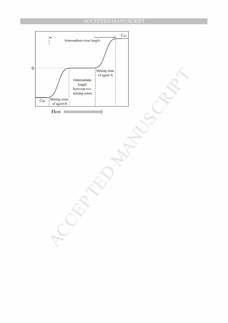
The study of mixing length is important for intermediate rinses, especially for long pipes. The usual 320

practice is to completely displace the cleaning agent A by water before introducing another cleaning 321

agent B. An alternative method is shown in Figure 10. Two cleaning agents can be synchronously 322

introduced with a proper interval between the agents. A so called intermediate rinse length is the sum 323

of the mixing zone length of the agent A, the mixing zone length of the agent B and an intermediate 324

length between two mixing zones. The intermediate length between two mixing zones can be 325

minimized in order to reduce water consumption. Thus, the minimum requirement of intermediate 326

rinsing water is the volume of two mixing zones which can be calculated from the mixing length. 327

Figure 11 demonstrates that the mixing length increases continuously with increasing rinsing time. The 328

leading edge (above 0) and trailing edge (below 0) are symmetrically located on two sides of the mid-329

plane. Zhao et al. (2010) also observed that the increase in flow velocities contributed to greater 330

mixing lengths when simulating the displacement of a heavier liquid A with another lighter liquid B in a 331

10 m straight pipe. 332

According to the penetration theory of Higbie (1935), the mixing length of different species is 333

dependent upon both the turbulent diffusivity and the contact time (van Elk et al., 2007; Zhao et al., 334

2010): 335

� ∝ 2Y�� ∙ � (7)

where � is the mixing length, �� is the turbulent diffusivity of the species. The right hand side term, 336

2Y�� ∙ � , is called characteristic length in mixing (Ekambara and Joshi, 2004). By replacing the 337

turbulent diffusivity with the axial dispersion coefficient, equation 7 also applies to the axial mixing of 338

CFD results as shown in Figure 12. The idea behind the correlation is that the penetration theory 339

quantifies the component transfer using a similar error function as in equation 1 (Assar et al., 2014). 340

MANUSCRIP

T

ACCEPTED

ACCEPTED MANUSCRIPT

19

On the basis of the correlation, it enables to predict the mixing lengths for longer rinsing time and 341

various flow rates and pipe diameters. 342

For a given pipe length, the contacting time can be assumed as ! ��⁄ , which is the mean residence 343

time of rinsing water. Then the minimum requirement of intermediate rinsing water can be calculated 344

from the mixing length, as: 345

������.����� = 2 ∙ V�>

4 ∙ � = 2 ∙ V�>

4 ∙ 3.29 ∙ Z2Y ∙ ! ��⁄ [ = 3.29V�>Y ∙ ! ��⁄ (8)

Under the flow conditions in this study, the second right hand side term in equation 3 dominates the 346

value of . Therefore, equation 8 can be further simplified and approximated as: 347

������.����� = 3.29V�>Y1.35(���)�.C=A(' (⁄ )�.�>A ∙ ! ��⁄

= 3.82VY���.\=A�].C=A(' (⁄ )�.�>A!

(9)

4. Application and further perspectives 348

4.1. Understand and control the process 349

The objective of any rinsing operation should be to completely remove the cleaning agent solution 350

using less water, shorter time and generating less wastewater. With this purpose in mind, the obtained 351

knowledge from this study can be categorized into two groups: the first type of knowledge is about 352

controlling the process, including the flow velocity, the minimum rinsing time and the times for 353

recovering the cleaning agent or rinsing water; the second type of knowledge is about understanding 354

the process, like the minimum water consumption, the minimum volume of wastewater, the recovered 355

volume of the cleaning agent and the minimum requirements of intermediate rinsing water. 356

Figure 13 presents an algorithm flowchart about how to apply the existing complex knowledge to 357

optimization of the rinsing process. Given the pipe diameter, flow velocity and pipe length, the 358

minimum rinsing time can be calculated. In practical cases, the real rinsing time is normally set with 359

MANUSCRIP

T

ACCEPTED

ACCEPTED MANUSCRIPT

20

safety margins, as it is not desired to risk producing inferior products due to unwise savings in 360

cleaning procedures. However, if the input rinsing time is much longer than the minimum required time, 361

it should be examined if an unnecessary waste of time and water is the case. 362

It is expensive to run CFD simulation for all conditions. But using the empirical or analytical equations 363

derived from CFD results is practical. Equation 4 calculates the time to stop the recovery of cleaning 364

agent and the time to start the recovery of rinsing water. Correspondingly, the effluent between the 365

two time points is regarded as wastewater, the minimum volume of which can be predicted with help 366

of equation 6. If the real volume of wastewater is more than the minimum, it means the recovery 367

efficiency can be higher by adjusting the recovery time. On the contrary, if the volume of wastewater is 368

less than the minimum, it leads to the potential risk of excessive recovery. For example, the recovered 369

cleaning agent has been diluted by the rinsing water, or the reused rinsing water has been “polluted” 370

by the cleaning agent. If it is the intermediate rinse between two cleaning agent solutions, the 371

minimum volume of intermediate rinsing water can be calculated according to equation 8 or 9. 372

4.2. A case study of rinsing a 24 m straight pipe with inner diameter 100 mm 373

The above results are extended to analyze the rinse of a 24 m straight pipe with inner diameter 100 374

mm. The mean flow velocity is 1 - 2 m/s. The set time of the rinsing step is assumed to be 1.5 ∙ ! ��⁄ . 375

In industrial practice, the rinsing time is usually set based on experience, which can thus be over or 376

below 1.5 times the residence time. The density and dynamic viscosity are assumed to be 997 kg/m3 377

and 8.899×10-4 kg/(m·s), and are assumed the same for the agent solution and the rinsing water. 378

Table 3 summarizes the results, which have been produced using the algorithm summarized in Figure 379

13. The calculated minimum rinsing time based on a fixed plane is 11.2% larger than the minimum 380

rinsing time calculated based on the volume. The set time is 1.36 times the ���,QROS��. The increase in 381

flow velocity can shorten the rinsing time. However, the consumption of rinsing water, the recovery of 382

MANUSCRIP

T

ACCEPTED

ACCEPTED MANUSCRIPT

21

cleaning agent and the generation of wastewater are independent of the flow velocities. The recovery 383

of cleaning agent is up to 89.3% of the volume. If it is the intermediate rinse, the increase in flow 384

velocity slightly reduces the minimum requirement of intermediate rinsing water. An important result is 385

that the implementation of synchronous intermediate rinse saves ~55% of water compared with the 386

minimum requirement to replace all agent components from the pipe. 387

4.3. Effects of complex element geometries 388

This study simulates the displacement process in straight pipes. However, a complete transfer line 389

consists of various elements, such as bends, T-joints, expansions, contractions and valves. Graßhoff 390

(1983) studied the displacement of one liquid with another liquid in three types of T-joints: (1) direct 391

entrance and exit with a perpendicular dead zone; (2) perpendicular entrance and exit with the dead 392

zone extending the entrance stream; and, (3) perpendicular entrance and exit with the dead zone 393

reversing the exit stream. A local sensor was installed at the end of the dead zone. With the increase 394

in the dead zone length from � to 10�, the displacement time (���) determined by the local sensor 395

varied from seconds to ten thousands of seconds. Thus, the time to completely remove the cleaning 396

agent from a long dead zone is much longer than for rinsing straight pipes. 397

CFD is a powerful tool to study the hygienic design of such elements. According to the European 398

Hygienic Engineering & Design Group (EHEDG) Testing and Certification guideline, CFD is currently 399

the only alternative to test the scalability of difference sizes of the same piece of equipment, apart 400

from the evaluation based on a design review and CIP test (EHEDG.org, 2016). CFD simulations of 401

the intermediate and final rinses serve as a supplement to previous studies where water is applied as 402

a medium to dissolve or remove soils from the surfaces (Asteriadou et al., 2009, 2007, 2006). This 403

article boosts the confidence to implement such CFD simulations of the displacement process for 404

more complex element geometries which are more commonly used in practice. 405

MANUSCRIP

T

ACCEPTED

ACCEPTED MANUSCRIPT

22

5. Conclusions 406

In this paper, CFD is used to simulate the intermediate and final rinses of straight horizontal pipes in 407

CIP applications. Axial mixing and displacement of agent solutions by water are studied and compared 408

with the Taylor model. The proposed CFD model for description of agent concentrations at varying 409

time points and locations in the pipe is found to give an excellent agreement with the Taylor analytical 410

model. 411

The key findings in the presented work are summarized in the following: 412

1) The displacement times are dependent on the pipe diameters and flow velocities. The product 413

of the displacement time and the mean flow velocity can be correlated by a power function with 414

inner pipe diameter as independent variable. 415

2) The minimum water consumption for completely rinsing a pipe is slightly larger than the pipe 416

volume. The minimum water consumption is not much influenced by changing flow velocities 417

when the flows are fully turbulent. 418

3) A practical rinsing step can be controlled based on downstream measurement and rinsing 419

stops when the measurement reaches the pre-defined criteria. However, the set time is still 420

longer than required. The water consumption is still more than the minimum requirement in 421

order to reduce contamination risks. 422

4) The minimum volume of wastewater can be predicted from the displacement times, and is 423

independent of the flow velocity. 424

5) Radial mixing is not significant during the displacement process. The mixing length varies with 425

the pipe diameters, flow velocities and rinsing time. The values of the mixing lengths are 426

proportional to the characteristic length (2√ ∙ � ), which can be applied to calculate the 427

minimum requirement of intermediate rinsing water. 428

MANUSCRIP

T

ACCEPTED

ACCEPTED MANUSCRIPT

23

The observations in this work can help to optimize the control of the rinsing step in terms of the flow 429

velocity, the rinsing time and the recovery plans of the cleaning agent and rinsing water. A case study 430

of rinsing a 24 m straight pipe with inner diameter 100 mm reveals that the recovery of cleaning agent 431

can be up to 89.3% of the volume and the saving of intermediate rinsing water can be at least 55%. 432

The successful simulation of the intermediate and final rinses of straight pipes builds confidence for 433

future studies to simulate the displacement process for more complex geometries and improve the 434

hygienic design and the CIP cleaning of different pipe elements. 435

Acknowledgements 436

This paper results from the DRIP (Danish partnership for Resource and water efficient Industrial food 437

Production) project. We acknowledge that this work is partly funded by the Innovation Fund Denmark 438

(IFD) under contract No. 5107-00003B, and by the Technical University of Denmark (DTU). 439

440

441

MANUSCRIP

T

ACCEPTED

ACCEPTED MANUSCRIPT

24

References 442

Assar, M., Abolghasemi, H., Hamane, M.R., Hashemi, S.J., Fatoorehchi, H., 2014. A new approach to 443 analyze entrance region mass transfer within a falling film. Heat Mass Transf. 50, 651–660. 444 doi:10.1007/s00231-013-1263-3 445

Asteriadou, K., Hasting, A.P.M., Bird, M.R., Melrose, J., 2009. Exploring CFD solutions for coexisting 446 flow regimes in a T-piece. Chem. Eng. Technol. 32, 948–955. doi:10.1002/ceat.200900060 447

Asteriadou, K., Hasting, A.P.M., Bird, M.R., Melrose, J., 2006. Computational Fluid Dynamics for the 448 Prediction of Temperature Profiles and Hygienic Design in the Food Industry. Food Bioprod. 449 Process. 84, 157–163. doi:10.1205/fbp.04261 450

Asteriadou, K., Hasting, T., Bird, M., Melrose, J., 2007. Predicting cleaning of equipment using 451 computational fluid dynamics. J. Food Process Eng. 30, 88–105. doi:10.1111/j.1745-452 4530.2007.00103.x 453

Bailey, J.E., Ollis, D.F., 1986. Biochemical Engineering Fundamentals, 2nd ed. McGraw-Hill Education, 454 Singapore. 455

Chen, L., Chen, R., Yin, H., Sui, J., Lin, H., 2012. Cleaning in place with onsite-generated electrolysed 456 oxidizing water for water-saving disinfection in breweries. J. Inst. Brew. 118, 401–405. 457 doi:10.1002/jib.56 458

Chisti, Y., Moo-Young, M., 1994. Clean-in-place systems for industrial bioreactors: Design, validation 459 and operation. J. Ind. Microbiol. 13, 201–207. doi:10.1007/BF01569748 460

EHEDG.org, 2016. Frequently Asked Questions about EHEDG Testing and Certification [WWW 461 Document]. URL http://www.ehedg.org/index.php?nr=301&lang=en (accessed 10.17.16). 462

Ekambara, K., Joshi, J.B., 2004. Axial mixing in laminar pipe flows. Chem. Eng. Sci. 59, 3929–3944. 463 doi:10.1016/j.ces.2004.05.025 464

Friis, A., Jensen, B.B.B., 2002. Prediction of hygiene in food processing equipment using flow 465 modelling. Food Bioprod. Process. 80, 281–285. doi:10.1205/096030802321154781 466

Graßhoff, A., 1983. Toträume in CIP-gereinigten Rohrleitungssystemen. Dtsch. Milchwirtschaft 13, 467 407–412. 468

Henningsson, M., Regner, M., Östergren, K., Trägårdh, C., Dejmek, P., 2007. CFD simulation and 469 ERT visualization of the displacement of yoghurt by water on industrial scale. J. Food Eng. 80, 470 166–175. doi:10.1016/j.jfoodeng.2006.04.058 471

Higbie, R., 1935. The rate of absorption of a pure gas into still liquid during short periods of exposure. 472 Trans. Am. Inst. Chem. Eng. 31, 365–389. 473

Jensen, B.B.B., 2007. Numerical study of influence of inlet turbulence parameters on turbulence 474 intensity in the flow domain: incompressible flow in pipe system. Proc. Inst. Mech. Eng. Part E J. 475 Process Mech. Eng. 221, 177–186. doi:10.1243/09544089JPME124 476

Jensen, B.B.B., Benezech, T., Legentilhomme, P., Lelievre, C., Friis, A., 2006. Predicting cleaning: 477

MANUSCRIP

T

ACCEPTED

ACCEPTED MANUSCRIPT

25

Estimate fluctuations in signal from electrochemical wall shear stress measurements using CFD, 478 in: Fouling, Cleaning & Disinfection in Food Processing. Department of Chemical Engineering, 479 University of Cambridge, Cambridge, UK. 480

Jensen, B.B.B., Friis, A., 2005. Predicting the cleanability of mix-proof valves by use of wall shear 481 stress. J. Food Process Eng. 28, 89–106. doi:10.1111/j.1745-4530.2005.00370.x 482

Jensen, B.B.B., Friis, A., 2004. Prediction of flow in mix-proof valve by use of CFD - validation by LDA. 483 J. Food Process Eng. 27, 65–85. doi:10.1111/j.1745-4530.2004.tb00623.x 484

Jurado-Alameda, E., Altmajer Vaz, D., Garcia Román, M., Siqueira Curto Valle, R.D.C., 2016. 485 Cleaning of starchy soils in Clean-in-Place (CIP) systems: relationship between contact angle 486 and detergency. J. Dispers. Sci. Technol. 37, 317–325. doi:10.1080/01932691.2014.1003223 487

Lelieveld, H.L.M., Mostert, M.A., Holah, J., 2005. Handbook of hygiene control in the food industry. 488 Woodhead Publishing Limited, Cambridge, UK. 489

Levenspiel, O., 1958. Longitudinal mixing of fluids flowing in circular pipes. Ind. Eng. Chem. 50, 343–490 346. doi:10.1021/ie50579a034 491

Li, G., Hall, P., Miles, N., Wu, T., 2015a. Improving the efficiency of “Clean-In-Place” procedures using 492 a four-lobed swirl pipe: A numerical investigation. Comput. Fluids 108, 116–128. 493 doi:10.1016/j.compfluid.2014.11.032 494

Li, G., Hall, P., Miles, N., Wu, T., 2015b. Optimization of a four-lobed swirl pipe for Clean-In-Place 495 procedures. Int. J. Environ. 9, 689–697. doi:10.13140/RG.2.1.4838.0004 496

Palabiyik, I., 2013. Investigation of fluid mechanical removal in the cleaning process. School of 497 Chemical Engineering, PhD thesis, University of Birmingham. 498

Palabiyik, I., Yilmaz, M.T., Fryer, P.J., Robbins, P.T., Toker, Ö.S., 2015. Minimising the environmental 499 footprint of industrial-scaled cleaning processes by optimisation of a novel clean-in-place system 500 protocol. J. Clean. Prod. 108, 1009–1018. doi:10.1016/j.jclepro.2015.07.114 501

Salmi, T., Mikkola, J.-P., Warna, P., 2010. Chemical reaction engineering and reactor technology. 502 CRC Press, Boca Raton. 503

Schöler, M., Föste, H., Helbig, M., Gottwald, A., Friedrichs, J., Werner, C., Augustin, W., Scholl, S., 504 Majschak, J.-P., 2012. Local analysis of cleaning mechanisms in CIP processes. Food Bioprod. 505 Process. 90, 858–866. doi:10.1016/j.fbp.2012.06.005 506

Sugiharto, Stegowski, Z., Furman, L., Su’ud, Z., Kurniadi, R., Waris, A., Abidin, Z., 2013. Dispersion 507 determination in a turbulent pipe flow using radiotracer data and CFD analysis. Comput. Fluids 79, 508 77–81. doi:10.1016/j.compfluid.2013.03.009 509

Tamime, A.Y., 2008. Cleaning-in-Place: Dairy, Food and Beverage Operations, 3rd ed. Blackwell, Ayr, 510 UK. 511

Taylor, G.I., 1953. Dispersion of soluble matter in solvent flowing slowly through a tube. Proceeding R. 512 Soc. London, Ser. A, Math. Phys. Sci. 219, 186–203. doi:10.1098/rspa.1953.0139 513

van Elk, E.P., Knaap, M.C., Versteeg, G.F., 2007. Application of the penetration theory for gas–liquid 514

MANUSCRIP

T

ACCEPTED

ACCEPTED MANUSCRIPT

26

mass transfer without liquid bulk: differences with systems with a bulk. Chem. Eng. Res. Des. 85, 515 516–524. doi:10.1205/cherd06066 516

Wiklund, J., Stading, M., Trägårdh, C., 2010. Monitoring liquid displacement of model and industrial 517 fluids in pipes by in-line ultrasonic rheometry. J. Food Eng. 99, 330–337. 518 doi:10.1016/j.jfoodeng.2010.03.011 519

Wilcox, D.C., 2006. Turbulence Modeling for CFD, 3rd ed. DCW Industries, La Canada, CA. 520

Yang, J., 2017. A review of cleaning-in-place: industrial challenges and practices, in: Dam-Johansen, 521 K., Forero-Hernández, H., Szabo, P. (Eds.), Graduate Schools Yearbook 2016. Technical 522 University of Denmark, Lyngby, pp. 151–152. 523

Zhao, L., Derksen, J., Gupta, R., 2010. Simulations of axial mixing of liquids in a long horizontal pipe 524 for industrial applications. Energy & Fuels 24, 5844–5850. doi:10.1021/ef100846r 525

526

MANUSCRIP

T

ACCEPTED

ACCEPTED MANUSCRIPT

Figure captions:

Figure 1. (A) The cleaning time of each step and (B) the costs in a CIP procedure of transfer pipes in a brewery. The cleaning is performed at room temperature. The recovery (~ 95%) of cleaning chemicals has been considered in the calculation of the costs. (Reproduced with permission of Carlsberg, Fredericia, Denmark)

Figure 2. Structured mesh of the cross section of the pipe with diameter 40.90 mm (DN 40). The near-wall meshes were enhanced by fine layers. The geometry was simplified as a quarter section of the pipe in order to save computational time. The mesh element in the pipe center (at the bottom-left corner) was nearly cuboid.

Figure 3. Description of the distribution of agent component within the pipe at � = 0. The agent components were dissolved in water with a concentration of 1 kg/m3 at � ≥ 0�. Water was flushed from � = −3�. Such treatment eliminated the entrance effect at � = 0 under which the inlet flow was not fully turbulent.

Figure 4. Near-wall turbulence intensity (1 mm from the wall) for different model cases. The inner pipe diameter is 40.90 mm (DN 40), the flow velocity is 1.5 m/s. The parameters of the 7 model cases are listed in Table 1. Cases 2, 6 and 7 are designed for the mesh independence study. Cases 1 – 5 are designed for the study of inlet boundary conditions. Case 2 is the reference which is the selected mesh.

Figure 5. Average agent concentrations at the different mid-planes (� = � ∙ �) for model cases as described in Table 1. The inner pipe diameter is 40.90 mm (DN 40), the flow velocity is 1.5 m/s. Equation 1 indicates that � = 0.5 �� ��⁄ at � = � ∙ �. Cases 1 - 5 result in the same average agent concentrations (with precision 0.00001 kg/m3), which are displayed as overlapping symbols.

Figure 6. Comparison of the Taylor model and the CFD simulations at 1.5 m/s of flow velocity for (A) a fixed distance of 15 m with varied rinsing time, and (B) a fixed rinsing time of 10 s with varied distance.

Figure 7. Axial velocity and turbulent kinetic energy at the distance of 15 m and for a mean flow velocity of 1.5 m/s for different pipe diameters (�� = 26500~259000). � ⁄ � is the dimensionless distance from the center of the pipe to the wall. The values of � and � quantify the intensity of convection in the axial direction when the radial velocity and tangential velocities are not significant in the pipe.

Figure 8. The product of displacement time and flow velocity for different pipe lengths. The marker values and error bars (too small to be seen) are from the CFD models for the simulated pipe diameters, representing the average and standard deviation of ���� ∙ � at three flow velocities. The curves represent the values which are calculated by the power function in equation 7.

Figure 9. Agent distribution in a 1 m pipe section at different rinsing times. The inner pipe diameter is 26.64 mm (DN 25 mm), and the flow velocity is 1.5 m/s.

Figure 10. Intermediate rinse length between two cleaning agents. The intermediate rinse length equals the sum of the mixing zone of agent A, the mixing zone of agent B and an intermediate length between two mixing zones. The minimum intermediate rinse length is when the intermediate length between two mixing zones is zero.

Figure 11. Dynamic mixing length of the 77.90 mm diameter (DN 80) pipe at 1 m/s and 2 m/s. ∆� is the relative position of the leading edge (+) and the trailing edge (−) to the mid-plane (� = � ∙ �)

MANUSCRIP

T

ACCEPTED

ACCEPTED MANUSCRIPT

Figure 12. Correlation of the mixing length with the characteristic length, 2√$ ∙ � . The mixing lengths of different pipe diameters at different flow velocities are proportional to the characteristic length, which can be expressed by a first order equation with high correlation coefficient.

Figure 13. The algorithm for understanding and controlling the rinse of straight pipes based on the findings in this study. The algorithm is only valid if the flow is turbulent.

MANUSCRIP

T

ACCEPTED

ACCEPTED MANUSCRIPT

Tables and captionss

Table 1. Parameters for the mesh study and for the influence of turbulence intensity and turbulence length scale. The inner pipe diameter is 40.90 mm (DN 40), the flow velocity is 1.5 m/s. Case 2 is the reference case which is selected for other studies.

Case Mesh

indexes

No. of nodes in radial / axial

directions

Tib

[%]

Tlb

[% of diameter] y+

Maximum Courant number

Mean Courant number

1 Mesh 1 21 / 501 1 10 45 0.69 0.26

2 Mesh 1 21 / 501 5 10 45 0.69 0.26

3 Mesh 1 21 / 501 20 10 45 0.70 0.26

4 Mesh 1 21 / 501 5 5 45 0.69 0.26

5 Mesh 1 21 / 501 5 30 45 0.69 0.26

6 Mesh 2 29 / 751 5 10 32 1.04 0.39

7 Mesh 3 27 / 501 5 10 4 0.81 0.24

MANUSCRIP

T

ACCEPTED

ACCEPTED MANUSCRIPT

Table 2. Correlation parameters of the product of displacement time and flow velocity for different pipe lengths by the power function as equation 7. The unit of inner pipe diameter should be meter. Depending on the practical cases, the correlation parameters of other pipe lengths can also be extracted from the CFD simulation results.

�, [�] �, [s] �, [��] � R2

2

��,� ��� 1.01 -0.121 0.998

���,� ��� 3.83 0.107 0.963

���,�� ��� 3.03 0.0788 0.966

15

��,� ��� 11.7 -0.0456 0.989

���,� ��� 19.1 0.0422 0.978

���,�� ��� 16.4 0.0212 0.970

24

��,� ��� 19.8 -0.0354 0.996

���,� ��� 29.1 0.0337 0.980

���,�� ��� 25.5 0.0152 0.971

MANUSCRIP

T

ACCEPTED

ACCEPTED MANUSCRIPT

Table 3. Result summary of the case study for rinsing a 24 m straight pipe with inner diameter 100 mm. The analysis follows the algorithm depicted in Figure 15.

��, [m/s] 1 1.5 2

Re 112035 168053 224070

Turbulence or not? Yes Yes Yes

�, [m2/s] 0.0316 0.0450 0.0579

��,� ���, [s] 21.43 14.29 10.72

���,� ���, [s] 31.43 20.95 15.71

���,�� ���, [s] 26.42 17.62 13.21

�� ��� 1.038 1.038 1.038

��� ��� 1.154 1.154 1.154

����,� ���, [m3] 0.218 0.218 0.218

����,�� ���, [m3] 0.196 0.196 0.196

����,� ��� ����,�� ���⁄ 1.112 1.112 1.112

Real rinsing time � = 1.5 ∙ � ��⁄ , [s] 36 24 18

�/���,�� ��� 1.36 1.36 1.36

Time to start the recovery of rinsing water, [s] 31.43 20.95 15.71

Real water consumption �#, [m3] 0.283 0.283 0.283

Recovery of cleaning agent solution, [m3] 0.168 0.168 0.168

Recovery percentage of cleaning agent solution, [%] 89.3 89.3 89.3

Minimum amount of wastewater, [m3] 0.079 0.079 0.079

���#�$.$��&�, [m3] 0.090 0.088 0.086

'����,�� ��� − ���#�$.$��&�) ����,�� ���* 0.539 0.551 0.559

MANUSCRIP

T

ACCEPTED

ACCEPTED MANUSCRIPT

MANUSCRIP

T

ACCEPTED

ACCEPTED MANUSCRIPT

MANUSCRIP

T

ACCEPTED

ACCEPTED MANUSCRIPT

MANUSCRIP

T

ACCEPTED

ACCEPTED MANUSCRIPT

MANUSCRIP

T

ACCEPTED

ACCEPTED MANUSCRIPT

MANUSCRIP

T

ACCEPTED

ACCEPTED MANUSCRIPT

MANUSCRIP

T

ACCEPTED

ACCEPTED MANUSCRIPT

MANUSCRIP

T

ACCEPTED

ACCEPTED MANUSCRIPT

MANUSCRIP

T

ACCEPTED

ACCEPTED MANUSCRIPT

MANUSCRIP

T

ACCEPTED

ACCEPTED MANUSCRIPT

MANUSCRIP

T

ACCEPTED

ACCEPTED MANUSCRIPT

MANUSCRIP

T

ACCEPTED

ACCEPTED MANUSCRIPT

MANUSCRIP

T

ACCEPTED

ACCEPTED MANUSCRIPT

MANUSCRIP

T

ACCEPTED

ACCEPTED MANUSCRIPT

MANUSCRIP

T

ACCEPTED

ACCEPTED MANUSCRIPT

MANUSCRIP

T

ACCEPTED

ACCEPTED MANUSCRIPT

Highlights

• CFD simulates the axial mixing which occurs during the intermediate and final rinses during cleaning of

straight pipes.

• The CFD results are in good agreement with the analytical models from literature.

• The model quantifies the minimum rinsing time, minimum water consumption and how to efficiently

recover the cleaning agent and rinsing water.

• An algorithm and a case study show how to use the investigated knowledge to solve practical problems.