Protons in Near Earth Orbit

The AMS Collaboration

Abstract

The proton spectrum in the kinetic energy range 0.1 to 200 GeV was measured bythe Alpha Magnetic Spectrometer (AMS) during space shuttle flight STS–91 at an alti-tude of 380 km. Above the geomagnetic cutoff the observed spectrum is parameterizedby a power law. Below the geomagnetic cutoff a substantial second spectrum was ob-served concentrated at equatorial latitudes with a flux∼70 m−2sec−1sr−1. Most of thesesecond spectrum protons follow a complicated trajectory and originate from a restrictedgeographic region.

Submitted toPhys. Lett. B

Introduction

Protons are the most abundant charged particles in space. The study of cosmic ray protons improvesthe understanding of the interstellar propagation and acceleration of cosmic rays.

There are three distinct regions in space where protons have been studied by different means:

• The altitudes of 30–40 km above the Earth’s surface. This region has been studied with balloonsfor several decades. Balloon experiments have made important contributions to the understand-ing of the primary cosmic ray spectrum of protrons and the behavior of atmospheric secondaryparticles in the upper layer of the atmosphere.

• The inner and outer radiation belts, which extend from altitudes of about 1000 km up to theboundary of the magnetosphere. Small size detectors on satellites have been sufficient to studythe high intensities in the radiation belts.

• A region intermediate between the top of the atmosphere and the inner radiation belt. Theradiation levels are normally not very high, so satellite-based detectors used so far,i.e. beforeAMS, have not been sensitive enough to systematically study the proton spectrum in this regionover a broad energy range.

Reference [?] includes some of the previous studies. The primary feature in the proton spectrumobserved near Earth is a low energy drop off in the flux, known as the geomagnetic cutoff. Thiscutoff occurs at kinetic energies ranging from∼10 MeV to ∼10 GeV depending on the latitude andlongitude. Above cutoff, from∼10 to∼100 GeV, numerous measurements indicate the spectrum fallsoff according to a power law.

The Alpha Magnetic Spectrometer (AMS) [?] is a high energy physics experiment scheduled forinstallation on the International Space Station. In preparation for this long duration mission, AMSflew a precursor mission on board the space shuttle Discovery during flight STS–91 in June 1998. Inthis report we use the data collected during the flight to study the cosmic ray proton spectrum fromkinetic energies of 0.1 to 200 GeV, taking advantage of the large acceptance, the accurate momentumresolution, the precise trajectory reconstruction and the good particle identification capabilities ofAMS.

The high statistics (∼ 107) available allow the variation of the spectrum with position to be mea-sured both above and below the geomagnetic cutoff. Because the incident particle direction and mo-mentum were accurately measured in AMS, it is possible to investigate the origin of protons belowcutoff by tracking them in the Earth’s magnetic field.

The AMS Detector

The major elements of AMS as flown on STS–91 consisted of a permanent magnet, a tracker, timeof flight hodoscopes, a Cerenkov counter and anticoincidence counters [?]. The permanent magnethad the shape of a cylindrical shell with inner diameter 1.1 m, length 0.8 m and provided a centraldipole field of 0.14 Tesla across the magnet bore and an analysing power,BL2, of 0.14 Tm2 parallelto the magnet, or z–, axis. The six layers of double sided silicon tracker were arrayed transverseto the magnet axis. The outer layers were just outside the magnet cylinder. The tracker measuredthe trajectory of relativistic singly charged particles with an accuracy of 20 microns in the bendingcoordinate and 33 microns in the non-bending coordinate, as well as providing multiple measurementsof the energy loss. The time of flight system had two planes at each end of the magnet, covering the

2

outer tracker layers. Together the four planes measured singly charged particle transit times with anaccuracy of 120 psec and also yielded multiple energy loss measurements. The Aerogel Cerenkovcounter (n = 1.035) was used to make independent velocity measurements to separate low energyprotons from pions and electrons. A layer of anticoincidence scintillation counters lined the innersurface of the magnet. Low energy particles were absorbed by thin carbon fiber shields. In flight theAMS positive z–axis pointed out of the shuttle payload bay.

For this study the acceptance was restricted to events with an incident angle within32◦ of thepositive z–axis of AMS and data from two periods are included. In the first period the z–axis waspointing within1◦ of the zenith. Events from this period are referred to as “downward” going. In thesecond period the z–axis pointing was within1◦ of the nadir. Data from this period are referred to as“upward” going. The orbital inclination was51.7◦ and the geodetic altitude during these two periodsranged from 350 to 390 km. Data taken while orbiting in or near the South Atlantic Anomaly wereexcluded.

The response of the detector was simulated using the AMS detector simulation program, based onthe GEANT package [?]. The effects of energy loss, multiple scattering, interactions, decays and themeasured detector efficiency and resolution were included.

The AMS detector was extensively calibrated at two accelerators: at GSI, Darmstadt, with heliumand carbon beams at 600 incident angles and locations and107 events, and at the CERN proton-synchrotron in the energy region of 2 to 14 GeV, with 1200 incident angles and locations and108

events. This ensured that the performance of the detector and the analysis procedure were thoroughlyunderstood.

Analysis

Reconstruction of the incident particle type, energy and direction started with a track finding proce-dure which included cluster finding, cluster coordinate transformation and pattern recognition. Thetrack was then fit using two independent algorithms [?, ?]. For a track to be accepted the fit wasrequired to include at least 4 hits in the bending plane and at least 3 hits in the non-bending plane.

The track was then extrapolated to each time of flight plane and matched with the nearest hit if itwas within 60 mm. Matched hits were required in at least three of the four time of flight planes. Thevelocity,β = v/c, was then obtained using this time of flight information and the trajectory. For eventswhich passed through the Cerenkov counter sensitive volume an independent velocity measurement,βC, was also determined. To obtain the magnitude of the particle charge,|Z|, a set of reference distri-butions of energy losses in both the time of flight and the tracker layers were derived from calibrationmeasurements made at the CERN test beam interpolated via the Monte Carlo method. For each eventthese references were fit to the measured energy losses using a maximum likelihood method. Thetrack parameters were then refit with the measuredβ andZ and the particle type determined from theresultantZ, β , βC and rigidity, R= pc/|Z|e(GV).

As protons and helium nuclei are the dominant components in cosmic rays, after selecting eventswith Z = +1 the proton sample has only minor backgrounds which consist of charged pions anddeuterons. The estimated fraction of charged pions, which are produced in the top part of AMS,with energy below 0.5 GeV is 1 %. Above this energy the fraction decreases rapidly with increasingenergy. The deuteron abundance in cosmic rays above the geomagnetic cutoff is about 2 %. Toremove low energy charged pions and deuterons the measured mass was required to be within 3standard deviations of the proton mass. This rejected about 3 % of the events while reducing thebackground contamination to negligible levels over all energies.

3

To determine the differential proton fluxes from the measured counting rates requires the ac-ceptance to be known as a function of the proton momentum and direction. Protons with differentmomenta and directions were generated via the Monte Carlo method, passed through the AMS de-tector simulation program and accepted if the trigger and reconstruction requirements were satisfiedas for the data. The acceptance was found to be 0.15 m2sr on average, varying from 0.3 to 0.03 m2srwith incident angle and location and only weakly momentum dependent. These acceptances werethen corrected following an analysis of unbiased trigger events. The corrections to the central valueare shown in Table 1 together with their contribution to the total systematic error of 5 %.

Correction Amount UncertaintyTrigger:

4–Fold Coincidence – 3 1.5Time of Flight Pattern – 4 2Tracker Hits – 2 1Anticoincidence 0 1

Analysis:Track and Velocity Fit – 2 1.5Particle Interactions + 1 1.5Proton Selection – 2 2

Monte Carlo Statistics 0 2Differential Acceptance Binning 0 2Total – 12 5

Table 1: Acceptance corrections and their systematic uncertainties, in percent

To obtain the incident differential spectrum from the measured spectrum, the effect of the detectorresolution was unfolded using resolution functions obtained from the simulation. These functionswere checked at several energy points by test beam measurements. The data were unfolded using amethod based on Bayes’ theorem [?, ?], which used an iterative procedure (and not a “regularizedunfolding”) to overcome instability of the matrix inversion due to negative terms. Fig. 1 compares thedifferential proton spectrum before and after unfolding in the geomagnetic equatorial region, definedbelow.

Results and Interpretation

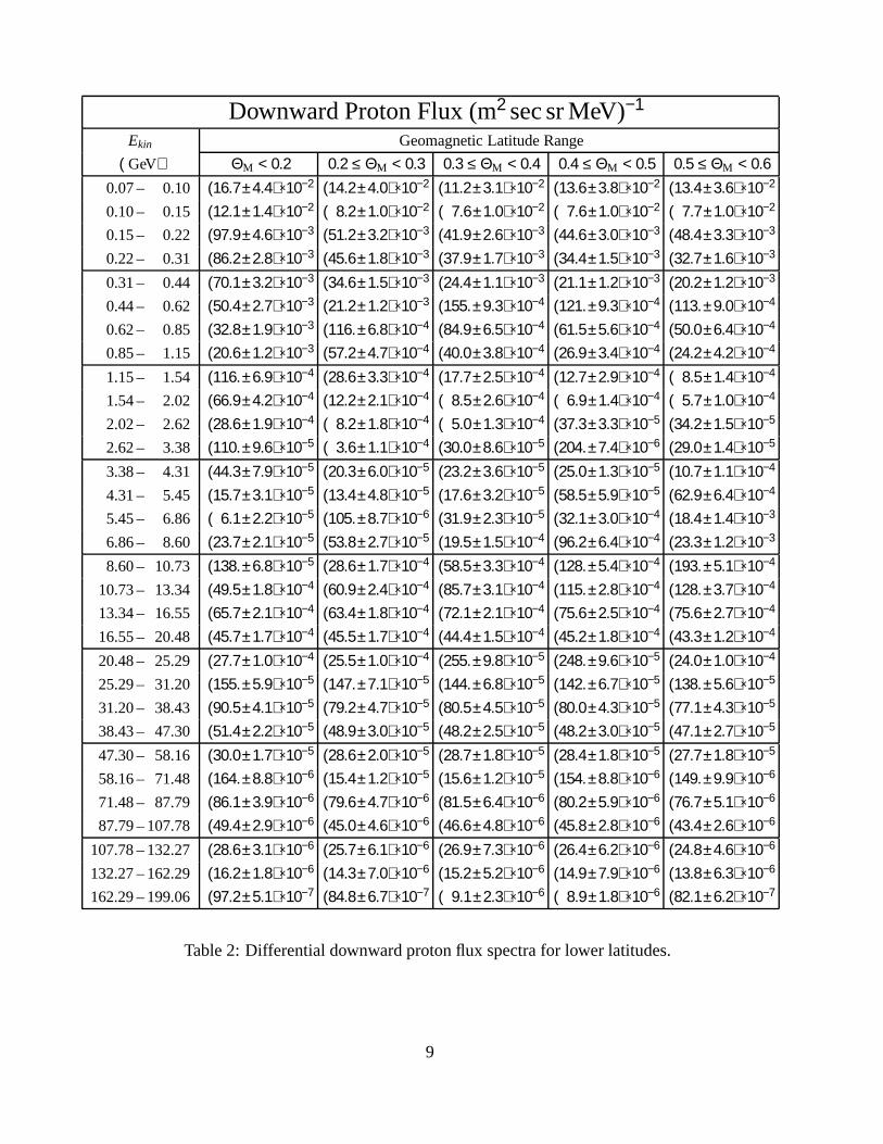
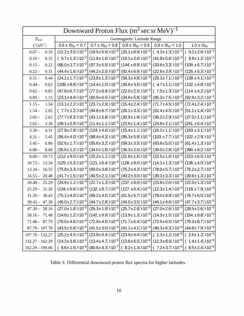
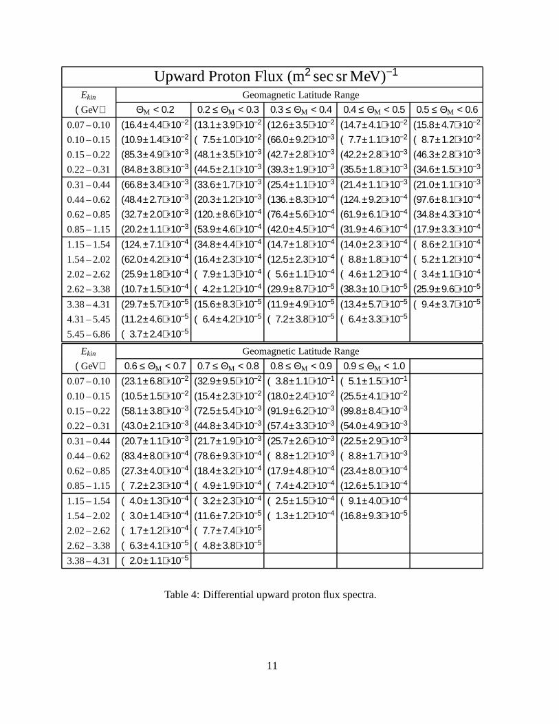
The differential spectra in terms of kinetic energy for downward and upward going protons integratedover incident angles within 32◦ of the AMS z–axis, which was within 1◦ of the zenith or nadir, arepresented in Fig. 2 and Tables 2–4. The results have been separated according to the absolute value ofthe corrected geomagnetic latitude [?], ΘM (radians), at which they were observed. Figs. 2a, b and cclearly show the effect of the geomagnetic cutoff and the decrease in this cutoff with increasingΘM.The spectra above and below cutoff differ. The spectrum above cutoff is refered to as the “primary”spectrum and below cutoff as the “second” spectrum.

4

I. Properties of the Primary Spectrum

The primary proton spectrum may be parameterized by a power law in rigidity,Φ0 × R−γ . Fitting [?]the measured spectrum over the rigidity range10 < R < 200 GV, i.e. well above cutoff, yields:

γ = 2.79 ± 0.012 (fit) ± 0.019 (sys),

Φ0 = 16.9 ± 0.2 (fit) ± 1.3 (sys) ± 1.5 (γ )GV2.79

m2sec sr MV.

The systematic uncertainty inγ was estimated from the uncertainty in the acceptance (0.006), thedependence of the resolution function on the particle direction and track length within one sigma(0.015), variation of the tracker bending coordinate resolution by± 4 microns (0.005) and variation ofthe selection criteria (0.010). The third uncertainty quoted forΦ0 reflects the systematic uncertaintyin γ .

II. Properties of the Second Spectrum

As shown in Figs. 2a, b, c, a substantial second spectrum of downward going protons is observedfor all but the highest geomagnetic latitudes. Figs. 2d, e, f show that a substantial second spectrumof upward going protons is also observed for all geomagnetic latitudes. The upward and downwardgoing protons of the second spectrum have the following unique properties:

(i) At geomagnetic equatorial latitudes,ΘM < 0.2, this spectrum extends from the lowest measuredenergy, 0.1 GeV, to∼6 GeV with a flux∼70 m−2sec−1sr−1.

(ii) As seen in Figs. 2a, d, the second spectrum has a distinct structure near the geomagnetic equa-tor: a change in geomagnetic latitude from 0 to 0.3 causes the proton flux to drop by a factor of2 to 3 depending on the energy.

(iii) Over the much wider interval0.3 < ΘM < 0.8, the flux is nearly constant.

(iv) In the range0 ≤ ΘM < 0.8, detailed comparison in different latitude bands (Fig. 3) indicatesthat the upward and downward fluxes are nearly identical, agreeing within 1 %.

(v) At polar latitudes,ΘM > 1.0, the downward second spectrum (Fig. 2c) is gradually obscured bythe primary spectrum, whereas the second spectrum of upward going protons (Fig. 2f) is clearlyobserved.

To understand the origin of the second spectrum, we traced [?] back105 protons from their mea-sured incident angle, location and momentum, through the geomagnetic field [?] for 10 sec flight timeor until they impinged on the top of the atmosphere at an altitude of 40 km, which was taken to be thepoint of origin. All second spectrum protons were found to originate in the atmosphere, except for fewpercent of the total detected near the South Atlantic Anomaly (SAA). These had closed trajectoriesand hence may have been circulating for a very long time and it is obviously difficult to trace back tothier origin. This type of trajectory was only observed near the SAA, clearly influenced by the innerradiation belt. To avoid confusion data taken in the SAA region were excluded though the rest of theprotons detected near the SAA had characteristics as the rest of the sample. Defining the flight timeas the interval between production and detection, Fig. 4 shows the distribution of momentum versusflight time of the remaining protons.

5

As seen in Fig. 4, the trajectory tracing shows that about 30 % of the detected protons flew forless than 0.3 sec before detection. The origin of these “short–lived” protons is distributed uniformlyaround the globe, see Fig. 5a, the apparent structure reflecting the orbits of the space shuttle. Incontrast, Fig. 5b shows that the remaining 70 % of protons with flight times greater than 0.3 sec,classified as “long–lived”, originate from a geographically restricted zone. Fig. 6 shows the stronglypeaked distribution of the point of origin of these long–lived protons in geomagnetic coordinates.Though data is presented only for protons detected atΘM < 0.3, these general features hold true upto ΘM ∼ 0.7. Fig. 7 shows the distribution of the number of geomagnetic equator crossings for long–lived and short–lived protons. About 15 % of all the second spectrum protons were detected on theirfirst bounce over the geomagnetic equator.

The measurements by AMS in near Earth orbit (at 380 km from the Earth’s surface), between theatmosphere and the radiation belt, show that the particles in this region follow a complicated path inthe Earth’s magnetic field. This behavior is different from that extrapolated from satellite observationsin the radiation belts, where the protons bounce across the equator for a much longer time. It is alsodifferent from that extrapolated from balloon observations in the upper layer of the atmosphere, wherethe protons typically cross the equator once. A striking feature of the second spectrum is that most ofthe protons originate from a restricted geographic region.

Acknowledgements

The support of INFN, Italy, ETH–Z¨urich, the University of Geneva, the Chinese Academy of Sci-ences, Academia Sinica and National Central University, Taiwan, the RWTH–Aachen, Germany, theUniversity of Turku, the University of Technology of Helsinki, Finland, the U.S. DOE and M.I.T.,CIEMAT, Spain, LIP, Portugal and IN2P3, France, is gratefully acknowledged.

We thank Professors S. Ahlen, C. Canizares, A. De Rujula, J. Ellis, A. Guth, M. Jacob, L. Maiani,R. Mewaldt, R. Orava, J. F. Ormes and M. Salamon for helping us to initiate this experiment.

The success of the first AMS mission is due to many individuals and organizations outside ofthe collaboration. The support of NASA was vital in the inception, development and operation ofthe experiment. The dedication of Douglas P. Blanchard, Mark J. Sistilli, James R. Bates, KennethBollweg and the NASA and Lockheed–Martin Mission Management team, the support of the Max–Plank Institute for Extraterrestrial Physics, the support of the space agencies from Germany (DLR),Italy (ASI), France (CNES) and China and the support of CSIST, Taiwan, made it possible to completethis experiment on time.

The support of CERN and GSI–Darmstadt, particularly of Professor Hans Specht and Dr. Rein-hard Simon made it possible for us to calibrate the detector after the shuttle returned from orbit.

The back tracing was made possible by the work of Professors E. Fl¨uckiger, D. F. Smart and M. A.Shea.

We are most grateful to the STS–91 astronauts, particularly to Dr. Franklin Chang–Diaz whoprovided vital help to AMS during the flight.

6

The AMS Collaboration

J.Alcaraz,y D.Alvisi,j B.Alpat,ac G.Ambrosi,r H.Anderhub,ag L.Ao,g A.Arefiev,ab P.Azzarello,r

E.Babucci,ac L.Baldini,j,l M.Basile,j D.Barancourt,s F.Barao,w,v G.Barbier,s G.Barreira,w R.Battiston,ac

R.Becker,lU.Becker,l L.Bellagamba,j P.Bene,r J.Berdugo,y P.Berges,l B.Bertucci,ac A.Biland,ag

S.Bizzaglia,ac S.Blasko,ac G.Boella,z M.Boschini,z M.Bourquin,r G.Bruni,j M.Buenerd,s J.D.Burger,l

W.J.Burger,ac X.D.Cai,l R.Cavalletti,j C.Camps,b P.Cannarsa,ag M.Capell,l D.Casadei,j J.Casaus,y

G.Castellini,p Y.H.Chang,m H.F.Chen,t H.S.Chen,i Z.G.Chen,g N.A.Chernoplekov,aa A.Chiarini,j

T.H.Chiueh,m Y.L.Chuang,ad F.Cindolo,j V.Commichau,b A.Contin,j A.Cotta–Ramusino,j P.Crespo,w

M.Cristinziani,r J.P.da Cunha,n T.S.Dai,l J.D.Deus,v N.Dinu,ac,1 L.Djambazov,ag I.D’Antone,j Z.R.Dong,h

P.Emonet,r J.Engelberg,u F.J.Eppling,l T.Eronen,aƒ G.Esposito,ac P.Extermann,r J.Favier,c C.C.Feng,x

E.Fiandrini,ac F.Finelli,j P.H.Fisher,l R.Flaminio,c G.Fluegge,b N.Fouque,c Yu.Galaktionov,ab,l

M.Gervasi,z P.Giusti,j D.Grandi,z W.Q.Gu,h K.Hangarter,b A.Hasan,ag V.Hermel,c H.Hofer,ag

M.A.Huang,ad W.Hungerford,ag M.Ionica,ac,1 R.Ionica,ac,1 M.Jongmanns,ag K.Karlamaa,u W.Karpinski,a

G.Kenney,ag J.Kenny,ac W.Kim,ae A.Klimentov,l,ab R.Kossakowski,c V.Koutsenko,l,ab G.Laborie,s

T.Laitinen,aƒ G.Lamanna,ac G.Laurenti,j A.Lebedev,l S.C.Lee,ad G.Levi,j P.Levtchenko,ac,2 C.L.Liu,x

H.T.Liu,i M.Lolli,j I.Lopes,n G.Lu,g Y.S.Lu,i K.Lubelsmeyer,a D.Luckey,l W.Lustermann,ag C.Mana,y

A.Margotti,j F.Massera,j F.Mayet,s R.R.McNeil,e B.Meillon,s M.Menichelli,ac F.Mezzanotte,j

R.Mezzenga,ac A.Mihul,k G.Molinari,j A.Mourao,v A.Mujunen,u F.Palmonari,j G.Pancaldi,j A.Papi,ac

I.H.Park,ae M.Pauluzzi,ac F.Pauss,ag E.Perrin,r A.Pesci,j A.Pevsner,d R.Pilastrini,j M.Pimenta,w,v

V.Plyaskin,ab V.Pojidaev,ab H.Postema,l,3 V.Postolache,ac,1 E.Prati,j N.Produit,r P.G.Rancoita,z D.Rapin,r

F.Raupach,a S.Recupero,j D.Ren,ag Z.Ren,ad M.Ribordy,r J.P.Richeux,r E.Riihonen,aƒ J.Ritakari,u

U.Roeser,ag C.Roissin,s R.Sagdeev,o D.Santos,s G.Sartorelli,j A.Schultz von Dratzig,a G.Schwering,a

E.S.Seo,o V.Shoutko,l E.Shoumilov,ab R.Siedling,a D.Son,ae T.Song,h M.Steuer,l G.S.Sun,h H.Suter,ag

X.W.Tang,i Samuel C.C.Ting,l S.M.Ting,l M.Tornikoski,u G.Torromeo,j J.Torsti,aƒ J.Trumper,q

J.Ulbricht,ag S.Urpo,u I.Usoskin,z E.Valtonen,aƒ J.Vandenhirtz,a F.Velcea,ac,1 E.Velikhov,aa B.Verlaat,ag,4

I.Vetlitsky,ab F.Vezzu,s J.P.Vialle,c G.Viertel,ag D.Vite,r H.Von Gunten,ag S.Waldmeier Wicki,ag

W.Wallraff,a B.C.Wang,x J.Z.Wang,g Y.H.Wang,ad K.Wiik,u C.Williams,j S.X.Wu,l,m P.C.Xia,h J.L.Yan,g

L.G.Yan,h C.G.Yang,i M.Yang,i S.W.Ye,t,5 P.Yeh,ad Z.Z.Xu,t H.Y.Zhang,ƒ Z.P.Zhang,t D.X.Zhao,h

G.Y.Zhu,i W.Z.Zhu,g H.L.Zhuang,i A.Zichichi.j

a I. Physikalisches Institut, RWTH, D-52056 Aachen, Germany6

b III. Physikalisches Institut, RWTH, D-52056 Aachen, Germany6

c Laboratoire d’Annecy-le-Vieux de Physique des Particules, LAPP, F-74941 Annecy-le-Vieux CEDEX,France

e Louisiana State University, Baton Rouge, LA 70803, USAd Johns Hopkins University, Baltimore, MD 21218, USAƒ Center of Space Science and Application, Chinese Academy of Sciences, 100080 Beijing, Chinag Chinese Academy of Launching Vehicle Technology, CALT, 100076 Beijing, Chinah Institute of Electrical Engineering, IEE, Chinese Academy of Sciences, 100080 Beijing, Chinai Institute of High Energy Physics, IHEP, Chinese Academy of Sciences, 100039 Beijing, China7

j University of Bologna and INFN-Sezione di Bologna, I-40126 Bologna, Italyk Institute of Microtechnology, Politechnica University of Bucharest and University of Bucharest,

R-76900 Bucharest, Romanial Massachusetts Institute of Technology, Cambridge, MA 02139, USA

m National Central University, Chung-Li, Taiwan 32054n Laboratorio de Instrumentacao e Fisica Experimental de Particulas, LIP, P-3000 Coimbra, Portugalo University of Maryland, College Park, MD 20742, USAp INFN Sezione di Firenze, I-50125 Florence, Italy

7

q Max–Plank Institut fur Extraterrestrische Physik, D-85740 Garching, Germanyr University of Geneva, CH-1211 Geneva 4, Switzerlands Institut des Sciences Nucleaires, F-38026 Grenoble, Francet Chinese University of Science and Technology, USTC, Hefei, Anhui 230 029, China7

u Helsinki University of Technology, FIN-02540 Kylmala, Finlandv Instituto Superior T´ecnico, IST, P-1096 Lisboa, Portugalw Laboratorio de Instrumentacao e Fisica Experimental de Particulas, LIP, P-1000 Lisboa, Portugalx Chung–Shan Institute of Science and Technology, Lung-Tan, Tao Yuan 325, Taiwan 11529y Centro de Investigaciones Energ´eticas, Medioambientales y Tecnolog´ıcas, CIEMAT, E-28040 Madrid,

Spain8z INFN-Sezione di Milano, I-20133 Milan, Italy

aa Kurchatov Institute, Moscow, 123182 Russiaab Institute of Theoretical and Experimental Physics, ITEP, Moscow, 117259 Russiaac INFN-Sezione di Perugia and Universit´a Degli Studi di Perugia, I-06100 Perugia, Italy9

ad Academia Sinica, Taipei, Taiwanae Kyungpook National University, 702-701 Taegu, Koreaaƒ University of Turku, FIN-20014 Turku, Finlandag Eidgenossische Technische Hochschule, ETH Z¨urich, CH-8093 Z¨urich, Switzerland1 Permanent address: HEPPG, Univ. of Bucharest, Romania.2 Permanent address: Nuclear Physics Institute, St. Petersburg, Russia.3 Now at European Laboratory for Particle Physics, CERN, CH-1211 Geneva 23, Switzerland.4 Now at National Institute for High Energy Physics, NIKHEF, NL-1009 DB Amsterdam, The

Netherlands.5 Supported by ETH Z¨urich.6 Supported by the Deutsches Zentrum f¨ur Luft– und Raumfahrt, DLR.7 Supported by the National Natural Science Foundation of China.8 Supported also by the Comisi´on Interministerial de Ciencia y Tecnolog´ıa.9 Also supported by the Italian Space Agency.

8

Downward Proton Flux (m2 sec sr MeV)−1

Ekin Geomagnetic Latitude Range

( GeV) ΘM < 0.2 0.2 ≤ ΘM < 0.3 0.3 ≤ ΘM < 0.4 0.4 ≤ ΘM < 0.5 0.5 ≤ ΘM < 0.60.07 – 0.10 (16.7±4.4) ×10−2 (14.2±4.0) ×10−2 (11.2±3.1) ×10−2 (13.6±3.8) ×10−2 (13.4±3.6) ×10−2

0.10 – 0.15 (12.1±1.4) ×10−2 ( 8.2±1.0) ×10−2 ( 7.6±1.0) ×10−2 ( 7.6±1.0) ×10−2 ( 7.7±1.0) ×10−2

0.15 – 0.22 (97.9±4.6) ×10−3 (51.2±3.2) ×10−3 (41.9±2.6) ×10−3 (44.6±3.0) ×10−3 (48.4±3.3) ×10−3

0.22 – 0.31 (86.2±2.8) ×10−3 (45.6±1.8) ×10−3 (37.9±1.7) ×10−3 (34.4±1.5) ×10−3 (32.7±1.6) ×10−3

0.31 – 0.44 (70.1±3.2) ×10−3 (34.6±1.5) ×10−3 (24.4±1.1) ×10−3 (21.1±1.2) ×10−3 (20.2±1.2) ×10−3

0.44 – 0.62 (50.4±2.7) ×10−3 (21.2±1.2) ×10−3 (155.±9.3) ×10−4 (121.±9.3) ×10−4 (113.±9.0) ×10−4

0.62 – 0.85 (32.8±1.9) ×10−3 (116.±6.8) ×10−4 (84.9±6.5) ×10−4 (61.5±5.6) ×10−4 (50.0±6.4) ×10−4

0.85 – 1.15 (20.6±1.2) ×10−3 (57.2±4.7) ×10−4 (40.0±3.8) ×10−4 (26.9±3.4) ×10−4 (24.2±4.2) ×10−4

1.15 – 1.54 (116.±6.9) ×10−4 (28.6±3.3) ×10−4 (17.7±2.5) ×10−4 (12.7±2.9) ×10−4 ( 8.5±1.4) ×10−4

1.54 – 2.02 (66.9±4.2) ×10−4 (12.2±2.1) ×10−4 ( 8.5±2.6) ×10−4 ( 6.9±1.4) ×10−4 ( 5.7±1.0) ×10−4

2.02 – 2.62 (28.6±1.9) ×10−4 ( 8.2±1.8) ×10−4 ( 5.0±1.3) ×10−4 (37.3±3.3) ×10−5 (34.2±1.5) ×10−5

2.62 – 3.38 (110.±9.6) ×10−5 ( 3.6±1.1) ×10−4 (30.0±8.6) ×10−5 (204.±7.4) ×10−6 (29.0±1.4) ×10−5

3.38 – 4.31 (44.3±7.9) ×10−5 (20.3±6.0) ×10−5 (23.2±3.6) ×10−5 (25.0±1.3) ×10−5 (10.7±1.1) ×10−4

4.31 – 5.45 (15.7±3.1) ×10−5 (13.4±4.8) ×10−5 (17.6±3.2) ×10−5 (58.5±5.9) ×10−5 (62.9±6.4) ×10−4

5.45 – 6.86 ( 6.1±2.2) ×10−5 (105.±8.7) ×10−6 (31.9±2.3) ×10−5 (32.1±3.0) ×10−4 (18.4±1.4) ×10−3

6.86 – 8.60 (23.7±2.1) ×10−5 (53.8±2.7) ×10−5 (19.5±1.5) ×10−4 (96.2±6.4) ×10−4 (23.3±1.2) ×10−3

8.60 – 10.73 (138.±6.8) ×10−5 (28.6±1.7) ×10−4 (58.5±3.3) ×10−4 (128.±5.4) ×10−4 (193.±5.1) ×10−4

10.73 – 13.34 (49.5±1.8) ×10−4 (60.9±2.4) ×10−4 (85.7±3.1) ×10−4 (115.±2.8) ×10−4 (128.±3.7) ×10−4

13.34 – 16.55 (65.7±2.1) ×10−4 (63.4±1.8) ×10−4 (72.1±2.1) ×10−4 (75.6±2.5) ×10−4 (75.6±2.7) ×10−4

16.55 – 20.48 (45.7±1.7) ×10−4 (45.5±1.7) ×10−4 (44.4±1.5) ×10−4 (45.2±1.8) ×10−4 (43.3±1.2) ×10−4

20.48 – 25.29 (27.7±1.0) ×10−4 (25.5±1.0) ×10−4 (255.±9.8) ×10−5 (248.±9.6) ×10−5 (24.0±1.0) ×10−4

25.29 – 31.20 (155.±5.9) ×10−5 (147.±7.1) ×10−5 (144.±6.8) ×10−5 (142.±6.7) ×10−5 (138.±5.6) ×10−5

31.20 – 38.43 (90.5±4.1) ×10−5 (79.2±4.7) ×10−5 (80.5±4.5) ×10−5 (80.0±4.3) ×10−5 (77.1±4.3) ×10−5

38.43 – 47.30 (51.4±2.2) ×10−5 (48.9±3.0) ×10−5 (48.2±2.5) ×10−5 (48.2±3.0) ×10−5 (47.1±2.7) ×10−5

47.30 – 58.16 (30.0±1.7) ×10−5 (28.6±2.0) ×10−5 (28.7±1.8) ×10−5 (28.4±1.8) ×10−5 (27.7±1.8) ×10−5

58.16 – 71.48 (164.±8.8) ×10−6 (15.4±1.2) ×10−5 (15.6±1.2) ×10−5 (154.±8.8) ×10−6 (149.±9.9) ×10−6

71.48 – 87.79 (86.1±3.9) ×10−6 (79.6±4.7) ×10−6 (81.5±6.4) ×10−6 (80.2±5.9) ×10−6 (76.7±5.1) ×10−6

87.79 – 107.78 (49.4±2.9) ×10−6 (45.0±4.6) ×10−6 (46.6±4.8) ×10−6 (45.8±2.8) ×10−6 (43.4±2.6) ×10−6

107.78 – 132.27 (28.6±3.1) ×10−6 (25.7±6.1) ×10−6 (26.9±7.3) ×10−6 (26.4±6.2) ×10−6 (24.8±4.6) ×10−6

132.27 – 162.29 (16.2±1.8) ×10−6 (14.3±7.0) ×10−6 (15.2±5.2) ×10−6 (14.9±7.9) ×10−6 (13.8±6.3) ×10−6

162.29 – 199.06 (97.2±5.1) ×10−7 (84.8±6.7) ×10−7 ( 9.1±2.3) ×10−6 ( 8.9±1.8) ×10−6 (82.1±6.2) ×10−7

Table 2: Differential downward proton flux spectra for lower latitudes.

9

Downward Proton Flux (m2 sec sr MeV)−1

Ekin Geomagnetic Latitude Range

( GeV) 0.6 ≤ ΘM < 0.7 0.7 ≤ ΘM < 0.8 0.8 ≤ ΘM < 0.9 0.9 ≤ ΘM < 1.0 1.0 ≤ ΘM

0.07 – 0.10 (12.2±3.5) ×10−2 (18.5±5.9) ×10−2 (25.1±8.9) ×10−2 ( 4.3±1.3) ×10−1 ( 9.2±2.6) ×10−1

0.10 – 0.15 ( 9.7±1.3) ×10−2 (11.8±1.6) ×10−2 (19.1±2.6) ×10−2 (41.8±5.6) ×10−2 ( 9.8±1.2) ×10−1

0.15 – 0.22 (66.0±3.7) ×10−3 (97.3±5.9) ×10−3 (144.±8.9) ×10−3 (33.6±3.3) ×10−2 (109.±6.7) ×10−2

0.22 – 0.31 (44.4±1.6) ×10−3 (44.2±2.0) ×10−3 (92.4±6.9) ×10−3 (22.6±3.9) ×10−2 (126.±5.3) ×10−2

0.31 – 0.44 (24.1±1.7) ×10−3 (23.8±1.3) ×10−3 (58.3±4.8) ×10−3 (29.3±7.1) ×10−2 (139.±4.1) ×10−2

0.44 – 0.62 (108.±8.8) ×10−4 (14.4±1.0) ×10−3 (36.6±3.5) ×10−3 ( 4.7±1.1) ×10−1 (132.±4.8) ×10−2

0.62 – 0.85 (47.8±6.7) ×10−4 (77.2±6.9) ×10−4 (22.0±2.5) ×10−3 ( 7.5±1.3) ×10−1 (114.±4.2) ×10−2

0.85 – 1.15 (23.1±4.9) ×10−4 (60.9±6.5) ×10−4 (34.9±5.8) ×10−3 (85.3±7.5) ×10−2 (92.8±3.2) ×10−2

1.15 – 1.54 (13.1±2.2) ×10−4 (23.7±2.9) ×10−4 (15.4±2.4) ×10−2 (71.7±4.5) ×10−2 (72.4±2.4) ×10−2

1.54 – 2.02 ( 7.7±1.2) ×10−4 (44.8±6.7) ×10−4 (28.1±3.3) ×10−2 (52.4±4.5) ×10−2 (51.1±1.4) ×10−2

2.02 – 2.62 (77.7±8.3) ×10−5 (43.1±5.8) ×10−3 (30.9±1.8) ×10−2 (36.2±2.9) ×10−2 (37.0±1.1) ×10−2

2.62 – 3.38 (49.1±5.9) ×10−4 (11.4±1.1) ×10−2 (22.6±1.4) ×10−2 (24.8±2.1) ×10−2 (241.±6.4) ×10−3

3.38 – 4.31 (27.9±2.9) ×10−3 (124.±4.6) ×10−3 (15.4±1.1) ×10−2 (16.2±1.1) ×10−2 (163.±3.1) ×10−3

4.31 – 5.45 (56.4±4.0) ×10−3 (88.4±4.3) ×10−3 (95.3±5.9) ×10−3 (103.±7.7) ×10−3 (102.±2.9) ×10−3

5.45 – 6.86 (52.6±1.7) ×10−3 (55.6±3.2) ×10−3 (59.3±3.5) ×10−3 (63.8±5.0) ×10−3 (61.4±1.3) ×10−3

6.86 – 8.60 (35.6±1.2) ×10−3 (34.0±1.8) ×10−3 (36.3±2.6) ×10−3 (39.0±2.8) ×10−3 (390.±8.2) ×10−4

8.60 – 10.73 (212.±9.0) ×10−4 (20.2±1.1) ×10−3 (21.8±1.6) ×10−3 (22.5±1.6) ×10−3 (223.±6.5) ×10−4

10.73 – 13.34 (129.±5.3) ×10−4 (121.±6.4) ×10−4 (128.±8.0) ×10−4 (14.1±1.3) ×10−3 (136.±4.5) ×10−4

13.34 – 16.55 (75.8±3.3) ×10−4 (69.0±3.8) ×10−4 (75.2±4.3) ×10−4 (78.0±5.7) ×10−4 (76.2±2.7) ×10−4

16.55 – 20.48 (41.7±1.5) ×10−4 (40.5±2.1) ×10−4 (40.2±3.0) ×10−4 (39.3±3.3) ×10−4 (39.6±1.3) ×10−4

20.48 – 25.29 (24.9±1.1) ×10−4 (22.7±1.3) ×10−4 (237.±8.0) ×10−5 (23.8±2.0) ×10−4 (22.0±1.3) ×10−4

25.29 – 31.20 (134.±5.6) ×10−5 (132.±8.7) ×10−5 (127.±6.4) ×10−5 (12.3±1.4) ×10−4 (118.±7.9) ×10−5

31.20 – 38.43 (75.1±4.0) ×10−5 (69.2±4.5) ×10−5 (61.5±5.7) ×10−5 (78.0±8.8) ×10−5 (76.7±6.5) ×10−5

38.43 – 47.30 (46.0±2.7) ×10−5 (44.7±2.8) ×10−5 (44.0±3.5) ×10−5 (44.1±4.6) ×10−5 (47.7±3.7) ×10−5

47.30 – 58.16 (27.0±1.8) ×10−5 (26.3±1.9) ×10−5 (25.7±2.8) ×10−5 (27.0±2.6) ×10−5 (28.5±2.6) ×10−5

58.16 – 71.48 (14.6±1.2) ×10−5 (142.±9.9) ×10−6 (13.9±1.3) ×10−5 (14.3±1.5) ×10−5 (154.±9.8) ×10−6

71.48 – 87.79 (76.0±4.6) ×10−6 (72.9±4.5) ×10−6 (71.7±6.4) ×10−6 (72.5±6.5) ×10−6 (79.3±8.7) ×10−6

87.79 – 107.78 (43.5±5.8) ×10−6 (41.5±3.0) ×10−6 (41.1±4.1) ×10−6 (40.3±6.3) ×10−6 (44.8±7.9) ×10−6

107.78 – 132.27 (25.2±4.5) ×10−6 (23.9±4.4) ×10−6 (23.9±4.4) ×10−6 ( 2.3±1.2) ×10−5 ( 2.6±1.2) ×10−5

132.27 – 162.29 (14.3±3.9) ×10−6 (13.4±4.7) ×10−6 (13.6±6.5) ×10−6 (12.3±8.9) ×10−6 ( 1.4±1.4) ×10−5

162.29 – 199.06 ( 8.6±1.5) ×10−6 (80.6±4.3) ×10−7 ( 8.2±1.3) ×10−6 ( 7.2±3.7) ×10−6 ( 8.5±2.4) ×10−6

Table 3: Differential downward proton flux spectra for higher latitudes.

10

Upward Proton Flux (m2 sec sr MeV)−1

Ekin Geomagnetic Latitude Range

( GeV) ΘM < 0.2 0.2 ≤ ΘM < 0.3 0.3 ≤ ΘM < 0.4 0.4 ≤ ΘM < 0.5 0.5 ≤ ΘM < 0.60.07 – 0.10 (16.4±4.4) ×10−2 (13.1±3.9) ×10−2 (12.6±3.5) ×10−2 (14.7±4.1) ×10−2 (15.8±4.7) ×10−2

0.10 – 0.15 (10.9±1.4) ×10−2 ( 7.5±1.0) ×10−2 (66.0±9.2) ×10−3 ( 7.7±1.1) ×10−2 ( 8.7±1.2) ×10−2

0.15 – 0.22 (85.3±4.9) ×10−3 (48.1±3.5) ×10−3 (42.7±2.8) ×10−3 (42.2±2.8) ×10−3 (46.3±2.8) ×10−3

0.22 – 0.31 (84.8±3.8) ×10−3 (44.5±2.1) ×10−3 (39.3±1.9) ×10−3 (35.5±1.8) ×10−3 (34.6±1.5) ×10−3

0.31 – 0.44 (66.8±3.4) ×10−3 (33.6±1.7) ×10−3 (25.4±1.1) ×10−3 (21.4±1.1) ×10−3 (21.0±1.1) ×10−3

0.44 – 0.62 (48.4±2.7) ×10−3 (20.3±1.2) ×10−3 (136.±8.3) ×10−4 (124.±9.2) ×10−4 (97.6±8.1) ×10−4

0.62 – 0.85 (32.7±2.0) ×10−3 (120.±8.6) ×10−4 (76.4±5.6) ×10−4 (61.9±6.1) ×10−4 (34.8±4.3) ×10−4

0.85 – 1.15 (20.2±1.1) ×10−3 (53.9±4.6) ×10−4 (42.0±4.5) ×10−4 (31.9±4.6) ×10−4 (17.9±3.3) ×10−4

1.15 – 1.54 (124.±7.1) ×10−4 (34.8±4.4) ×10−4 (14.7±1.8) ×10−4 (14.0±2.3) ×10−4 ( 8.6±2.1) ×10−4

1.54 – 2.02 (62.0±4.2) ×10−4 (16.4±2.3) ×10−4 (12.5±2.3) ×10−4 ( 8.8±1.8) ×10−4 ( 5.2±1.2) ×10−4

2.02 – 2.62 (25.9±1.8) ×10−4 ( 7.9±1.3) ×10−4 ( 5.6±1.1) ×10−4 ( 4.6±1.2) ×10−4 ( 3.4±1.1) ×10−4

2.62 – 3.38 (10.7±1.5) ×10−4 ( 4.2±1.2) ×10−4 (29.9±8.7) ×10−5 (38.3±10.) ×10−5 (25.9±9.6) ×10−5

3.38 – 4.31 (29.7±5.7) ×10−5 (15.6±8.3) ×10−5 (11.9±4.9) ×10−5 (13.4±5.7) ×10−5 ( 9.4±3.7) ×10−5

4.31 – 5.45 (11.2±4.6) ×10−5 ( 6.4±4.2) ×10−5 ( 7.2±3.8) ×10−5 ( 6.4±3.3) ×10−5

5.45 – 6.86 ( 3.7±2.4) ×10−5

Ekin Geomagnetic Latitude Range

( GeV) 0.6 ≤ ΘM < 0.7 0.7 ≤ ΘM < 0.8 0.8 ≤ ΘM < 0.9 0.9 ≤ ΘM < 1.00.07 – 0.10 (23.1±6.8) ×10−2 (32.9±9.5) ×10−2 ( 3.8±1.1) ×10−1 ( 5.1±1.5) ×10−1

0.10 – 0.15 (10.5±1.5) ×10−2 (15.4±2.3) ×10−2 (18.0±2.4) ×10−2 (25.5±4.1) ×10−2

0.15 – 0.22 (58.1±3.8) ×10−3 (72.5±5.4) ×10−3 (91.9±6.2) ×10−3 (99.8±8.4) ×10−3

0.22 – 0.31 (43.0±2.1) ×10−3 (44.8±3.4) ×10−3 (57.4±3.3) ×10−3 (54.0±4.9) ×10−3

0.31 – 0.44 (20.7±1.1) ×10−3 (21.7±1.9) ×10−3 (25.7±2.6) ×10−3 (22.5±2.9) ×10−3

0.44 – 0.62 (83.4±8.0) ×10−4 (78.6±9.3) ×10−4 ( 8.8±1.2) ×10−3 ( 8.8±1.7) ×10−3

0.62 – 0.85 (27.3±4.0) ×10−4 (18.4±3.2) ×10−4 (17.9±4.8) ×10−4 (23.4±8.0) ×10−4

0.85 – 1.15 ( 7.2±2.3) ×10−4 ( 4.9±1.9) ×10−4 ( 7.4±4.2) ×10−4 (12.6±5.1) ×10−4

1.15 – 1.54 ( 4.0±1.3) ×10−4 ( 3.2±2.3) ×10−4 ( 2.5±1.5) ×10−4 ( 9.1±4.0) ×10−4

1.54 – 2.02 ( 3.0±1.4) ×10−4 (11.6±7.2) ×10−5 ( 1.3±1.2) ×10−4 (16.8±9.3) ×10−5

2.02 – 2.62 ( 1.7±1.2) ×10−4 ( 7.7±7.4) ×10−5

2.62 – 3.38 ( 6.3±4.1) ×10−5 ( 4.8±3.8) ×10−5

3.38 – 4.31 ( 2.0±1.1) ×10−5

Table 4: Differential upward proton flux spectra.

11

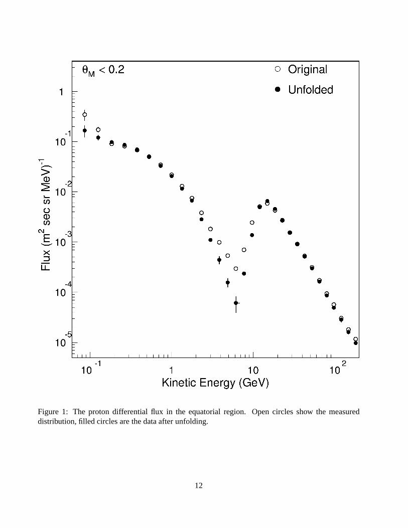
Figure 1: The proton differential flux in the equatorial region. Open circles show the measureddistribution, filled circles are the data after unfolding.

12

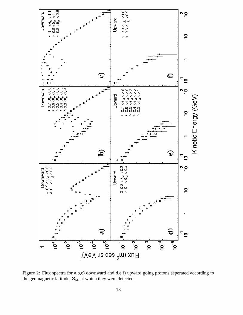
Figure 2: Flux spectra for a,b,c) downward and d,e,f) upward going protons seperated according tothe geomagnetic latitude,ΘM, at which they were detected.

13

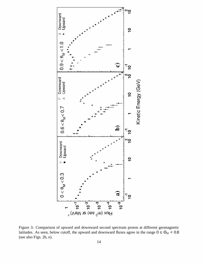
Figure 3: Comparison of upward and downward second spectrum proton at different geomagneticlatitudes. As seen, below cutoff, the upward and downward fluxes agree in the range0 ≤ ΘM < 0.8(see also Figs. 2b, e).

14

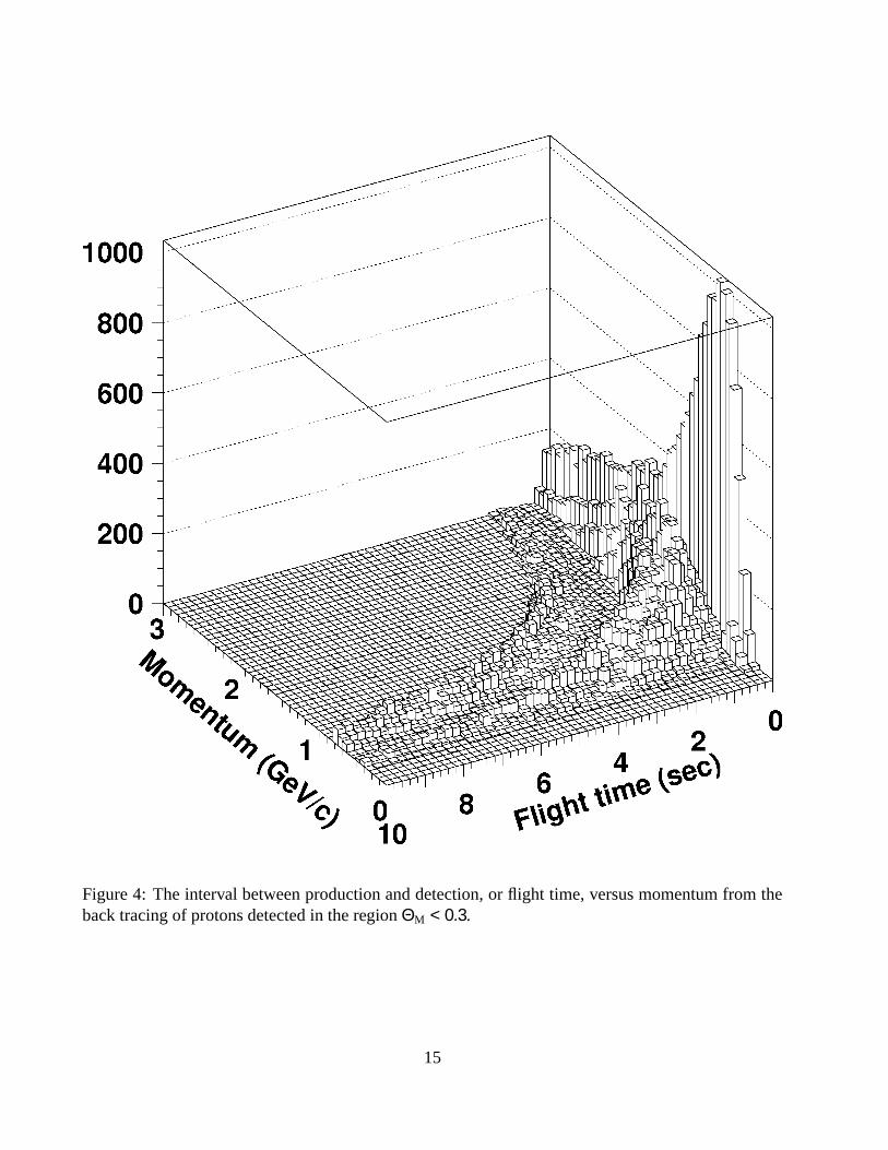
Figure 4: The interval between production and detection, or flight time, versus momentum from theback tracing of protons detected in the regionΘM < 0.3.

15

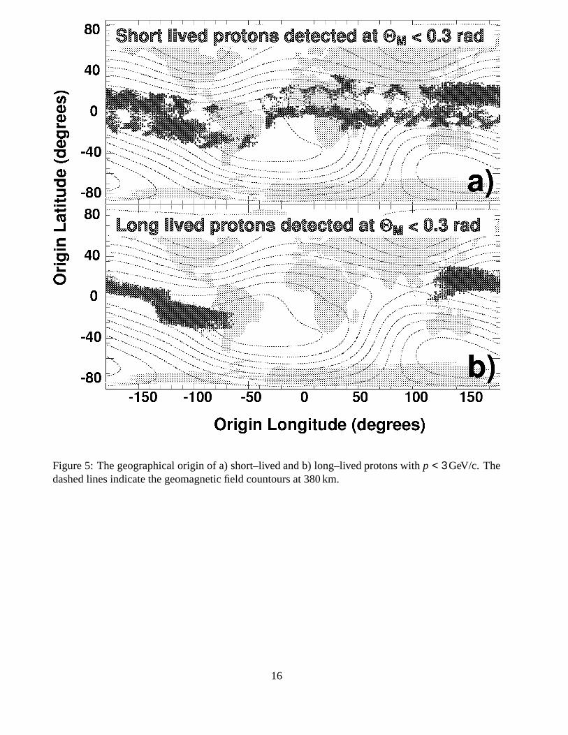
Figure 5: The geographical origin of a) short–lived and b) long–lived protons withp < 3 GeV/c. Thedashed lines indicate the geomagnetic field countours at 380 km.

16

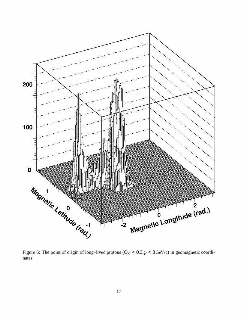
Figure 6: The point of origin of long–lived protons (ΘM < 0.3, p < 3 GeV/c) in geomagnetic coordi-nates.

17

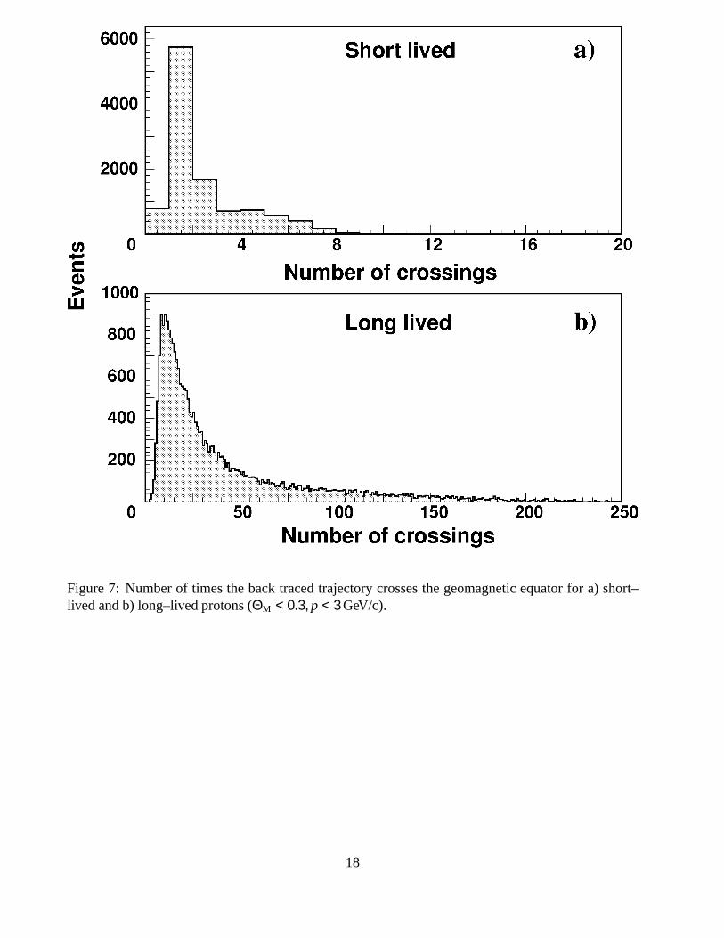
Figure 7: Number of times the back traced trajectory crosses the geomagnetic equator for a) short–lived and b) long–lived protons (ΘM < 0.3, p < 3 GeV/c).

18