arX

iv:c

ond-

mat

/061

2618

v1 [

cond

-mat

.sta

t-m

ech]

25

Dec

200

6

Barrier crossing driven by Levy noise: Universality and the Role of Noise Intensity

Aleksei V. Chechkin,1 Oleksii Yu. Sliusarenko,1 Ralf Metzler,2, 3 and Joseph Klafter4

1Institute for Theoretical Physics NSC KIPT, Akademicheskaya st.1, 61108 Kharkov, Ukraine2Dept of Physics, University of Ottawa - 150 Louis Pasteur, Ottawa, ON, K1N 6N5, Canada

3NORDITA—Nordic Institute for Theoretical Physics, Blegdamsvej 17, 2100 Copenhagen Ø, Denmark4School of Chemistry, Tel Aviv University, Ramat Aviv, Tel Aviv 69978, Israel

(Dated: 6th February 2008)

We study the barrier crossing of a particle driven by white symmetric Levy noise of index α andintensity D for three different generic types of potentials: (a) a bistable potential; (b) a metastablepotential; and (c) a truncated harmonic potential. For the low noise intensity regime we recover the

previously proposed algebraic dependence on D of the characteristic escape time, Tesc ≃ C(α)/Dµ(α),where C(α) is a coefficient. It is shown that the exponent µ(α) remains approximately constant,µ ≈ 1 for 0 < α < 2; at α = 2 the power-law form of Tesc changes into the known exponentialdependence on 1/D; it exhibits a divergence-like behavior as α approaches 2. In this regime weobserve a monotonous increase of the escape time Tesc with increasing α (keeping the noise intensityD constant). The probability density of the escape time decays exponentially. In addition, forlow noise intensities the escape times correspond to barrier crossing by multiple Levy steps. Forhigh noise intensities, the escape time curves collapse for all values of α. At intermediate noiseintensities, the escape time exhibits non-monotonic dependence on the index α, while still retainingthe exponential form of the escape time density.

PACS numbers: 05.40.Fb,02.50.-Ey,82.20.-w

I. INTRODUCTION

In his seminal paper [1], Kramers proposed to modelchemical reaction rates as the diffusion of a Brownianparticle, initially located in a potential well, across a po-tential barrier of finite height. Meanwhile, Kramers’ the-ory has been applied to a much more general range of pro-cesses associated with the barrier crossing of a physicalentity experiencing random kicks fuelled by its contactto a thermal bath [2–5].

Since Kramers’ solution numerous different ways havebeen reported to access the barrier crossing problem, inparticular, to find the mathematically most convenientformulation, compare, for instance, Refs. [3–6]. The re-sult for the characteristic escape time reads [7]

Tesc =2π exp ([U(xmax) − U(xmin)] /D)

√

U ′′ (xmin) |U ′′ (xmax)|(1)

where U (x) is the dimensionless potential, a prime standsfor the derivative with respect to the coordinate x; xmin

and xmax are the points, where the potential U (x) at-tains its minimum and maximum, respectively; and D isthe diffusion coefficient (noise intensity) of the diffusingparticle, stemming from its coupling to the heat bath.Eq. (1) is based on the assumption that the barrier ishigh (or equivalently, the noise intensity is low), and thereexists a constant probability flux across the barrier max-imum.

Random processes in complex systems frequently vio-late the rules of Brownian motion. Thus, the presenceof static or dynamic disorder might give rise to mem-ory effects causing subdiffusion [8, 9], and possible de-viations from standard exponential relaxation [10, 11].

The barrier crossing in the presence of long-range mem-ory effects was, inter alia, modeled in terms of a gener-alized Langevin equation [12, 13], or via a subdiffusivefractional kinetic approach with Mittag-Leffler survival[14, 15]. Subdiffusion is usually associated with a long-tailed waiting time distribution ψ(t) ∼ Aγτ

γ/t1+γ with0 < γ < 1 rendering the resulting continuous time ran-dom walk process semi-Markovian, its hallmark being thepower-law time-dependence 〈x2〉 ∝ Kγt

γ of the mean-squared displacement in absence of an external potential[8, 9, 16].

While in subdiffusion the waiting time between succes-sive jump events becomes modified such that the meanwaiting time

∫

∞

0tψ(t)dt diverges and consequently no

natural time scale separating microscopic and macro-scopic events exists, the distribution of the lengths of in-dividual jumps is narrow. The converse is true for Levyflights: Here, the lengths of the jumps are distributedaccording to the long-tailed jump length distribution

λ(x) ∼ Aασα

|x|1+α(2)

with 0 < α < 2 [8, 15, 17, 18]. Thus, the variance∫

∞

−∞x2λ(x)dx of the jump lengths diverges. Such power-

law forms of the jump lengths have been recognized in awide number of fields [9]. Prominent examples for suchgenuine Levy flights are known from noise patterns inplasma devices [19], and from random walks of particlesor excitations along a fastly folding polymer, where thewalker is allowed to cross the small gap between two seg-ments of the chain, that are close by in the embeddingspace due to polymer looping [20]. In the latter case, theexponent α is in fact related to the critical exponents ofthe polymer chain. Further examples come from fluctua-

2

tions in energy space in small systems [21, 22], and frompaleoclimatic time series [23].

From a mathematical point of view the occurrenceof long-tailed distributions appears quite natural dueto the Levy-Gnedenko generalized central limit theorem[24, 25]. Indeed, the tails of probability densities of thetype of λ(x), Eq. (2), are obtained from the characteris-tic function of a symmetric α-stable distribution of theform

λ(k) ≡ F{λ(x)} =

∫

∞

−∞

eikxλ(x)dx = exp (−c|k|α) ,

(3)where c > 0. The power-law asymptotics at large |x|,Eq. (2), appear immediately from the expansion of thecharacteristic function Eq. (3) in the limit of small k.

An important question arises when replacing the Brow-nian particle in a barrier crossing process by a particleexecuting Levy flights. This situation can be modelledby a particle subject to Levy stable noise, on the levelof the Langevin equation. First steps in this direction ofaddressing have been taken, as reported in Refs. [26–29].In the present work, we report extended simulations re-sults for the usually studied case of low noise strength D,observing a pronounced step-like behavior of the depen-dence of the exponent µ on the Levy index α. We alsoexplore the case of intermediate and high noise strength,finding a quite rich behavior in the parameter space, in-cluding an optimum α for the escape time.

II. UNDERLYING LANGEVIN EQUATION

We start from the Langevin equation for a particle em-bedded in an external potential field and subjected to arandom noise,

dx(t)

dt= − 1

mγ

dU(x)

dx+ ξα(t), (4)

where x(t) is the dynamic variable (particle position), mthe mass, γ the friction constant, and U(x) an externalpotential. The noise ξα(t) is a white, symmetric α-stablenoise. Eq. (4) is understood in the following way [30].Integrating Eq. (4) over the interval [t, t+∆t], we obtain

x(t+∆t)−x(t) = − 1

mγ

∫ t+∆t

t

dU(x(t′))

dxdt′+Lα,D(∆t),

(5)where

Lα,D(∆t) =

∫ t+∆t

t

ξα,D(t′)dt′ (6)

is an α-stable process with stationary independent incre-ments and characteristic function

pL(k,∆t) = exp (−D|k|α∆t) . (7)

D is the intensity of the Levy noise. With the use ofEqs. (6) and (7) it is straightforward to show [30] that the

discrete time representation of Eq. (5) at times tn = nδt,n = 0, 1, 2, . . . for sufficiently small time step δt is

xn+1 − xn = − 1

mγ

dU(xn)

dxδt+ (Dδt)1/α ξα,1(n), (8)

where {ξα,1(n)} is a set of random variables possess-ing Levy stable distribution λ(x) with the characteristicfunction (3) and c = 1.

III. SIMULATIONS RESULTS

Before addressing the barrier crossing problem in thepresence of Levy stable noise analytically below, wepresent results from extensive simulations. In these sim-ulations, we employ three types of potential profiles:bistable, metastable, and truncated harmonic potentials(see Fig.1) defined as follows:

U1(x) = −g1x2

2+ g2

x4

4; (9a)

U2(x) = −g1x3

3+ g2x (9b)

U3(x) =

{

g1x2/2, −L ≤ x ≤ L

0, |x| > L. (9c)

Let us turn to dimensionless variables. To this end wesubstitute x → x/x, t → t/t, and D → D/D into thediscrete time Langevin equation (8), and choose the ap-

propriate constants for rescaling, x, t, and D, for eachpotential type. Taking into account that ξα

(

t/t)

=

t1−1/αξα(t) [30], we find

x =

√

g2g1, t =

g1mγ

, D =mγ

g1

(

g2g1

)α/2

; (10a)

x =

√

g1g2, t =

√g1g2

mγ, D =

mγ√g1g2

(

g1g2

)α/2

;(10b)

x = L,xα

D= t =

mγ

g1, (10c)

respectively. In terms of these rescaled variables the dis-crete time Langevin equation (8) reads

xn+1 − xn = −dU(xn)

dxδt+ (Dδt)

1/αξα,1(n), (11)

where the potential U(xn) refers to, respectively, U1, U2,or U3 from Eqs. (9), with g1 = g2 = L = 1.

In the simulations, for each type of the potential theparticle starts from the bottom of the potential well. Theadsorbing boundary is located: (i) for the bistable poten-tial in the saddle point x = 0; (ii) for the metastable po-tential far to the right of the saddle point, at x = 10; and(iii) for the truncated harmonic potential at the bound-aries, |x| = 1. The process defined by Eq. (11) is repeated

3

xxx

UU U1 2 3

Figure 1: The three types of potential profiles U1 (bistable potential), U2 (metastable potential), and U3 (truncated harmonicpotential) considered in the simulations; for g1, g2, L > 0.

until the particle reaches, or crosses the adsorbing bound-ary; then the process in Eq. (11) is restarted. This proce-dure is performed 100,000 times, for fixed D and α, andthe mean escape time is then calculated [31].

The mean escape times Tesc of the diffusing particleas function of noise intensity D for the three potentialprofiles are shown in Fig. 2 for different values of α rang-ing from 0.1 to 2 [32]. It is clear that the curves forα < 2 obey a different law in comparison to their Gaus-sian counterpart. We observe three different regimes forthe dependence of Tesc on the Levy noise parameters,which can be classified by the value of noise intensity.Let us discuss these regimes in detail.

A. Low noise intensity regime

In this regime, instead of an exponential dependenceon 1/D, the curves shown in Fig. 2 display a power-lawasymptotic behavior of the mean escape time

Tesc(α,D) =C(α)

Dµ(α). (12)

Further analysis of the data plotted in Fig. 2 allows usto determine the dependencies of the power law expo-nent µ(α) and coefficient C(α) on the Levy index α (seeFig. 3). The exponent µ(α) is approximately unity up toα ≈ 1.5. The dependence of C(α) for the first two po-tential types possesses a weak inflection at small α. Notethat for fixed noise strength D, the dependence of Tesc

on the Levy index α is monotonic.Let us now turn to the probability density function

(PDF) p(t) of the escape times. We use again our simu-lation scheme to obtain p(t) from the Langevin equation(11), but now for each fixed values of α and D we collect200,000 escape events, which are not averaged but pro-cessed with a simple routine, that constructs the PDF.The results for the three potentials from Fig.1 are shownin Fig. 4 [34]. It is imminently clear that in all three

cases and for all α (including the Gaussian case, α = 2)the exponential decay pattern

p(t) =1

Texp

(

− t

T

)

(13)

is nicely obeyed, in agreement with the findings fromprevious simulations studies [23, 28, 29], as well as withthe analytical results reported in Ref. [26].

Relation (13) allows us to extract the mean escape timeTesc independently from our previous results in Fig. 2, intwo different ways. Namely, we define

Tesc =1

p(0)≡ T1; (14)

alternatively, we determine

Tesc = −(

d ln p(t)

dt

)

−1

≡ T2. (15)

These two ways to determine Tesc are intrinsically dif-ferent, T1 depending on the extrapolation of the fittedexponential behavior to t = 0, whereas T2 is determinedthrough the slope in the logarithmic versus linear plot.Tab. I shows the results for T1 and T2 along with the val-ues of Tesc obtained directly from the simulations resultsin Figs. 2. Indeed, the value of T2 is consistently closerto Tesc than T1. Overall, however, the agreement is verygood (better than 1.5 per cent).

B. High and intermediate noise intensity regimes

We consider these two regimes for the case of the trun-cated harmonic potential as example, compare to thebottom graph in Fig.2. The two other cases, bistableand metastable potentials, demonstrate similar behav-ior. When the noise intensity D increases beyond thelow noise limit, in which the curves exhibit a linear de-pendence and are almost parallel, the various curves for

4

0.1

0.1

0.1

Figure 2: Mean escape times as function of noise intensityD for the bistable (top), metastable (middle), and truncatedharmonic potentials (bottom).

the escape time show a tendency to collapse. This isthe intermediate noise intensity regime, which for thetruncated harmonic potential lies approximately in therange −2 < −lgD < 1. Here, we observe that Tesc

demonstrates very weak dependence on the Levy index,in comparison with the low intensity regime. The ex-

m(a

)

a

a

a

a

m(a

)

a

a

m(a

)

a

Figure 3: Dependencies of µ(α) and C(α) for the bistable(top), metastable (middle) and truncated harmonic (bottom)potentials. See text.

planation is the following. Contrary to the weak noiseintensity regime, where the tail of the Levy noise distri-bution plays a decisive role in the escape process (lessfrequent but high amplitude noise spikes, that is, governthe barrier crossing), here the main role in the process,due to the higher intensities, passes on to the central part

5

Figure 4: Escape time probability density functions in depen-dence of time for the bistable (top), metastable (middle) andtruncated harmonic (bottom) potentials. In the log versus linplot, the exponential dependence is obvious.

of the distribution. Since all stable distributions, includ-ing the Gaussian, have central parts which are of simi-lar shape, the α-dependence of the escape time becomesweaker. Furthermore, in the intermediate region we ob-serve a non-monotonic dependence of Tesc versus α, ex-amples for three values of D taken from the intermediateregime are shown in Fig. 5. This weak non-monotonicity

First potential type, D = 10−2.0

α Tesc T1 T2

0.1 119.7 117.4 118.1

0.5 187.1 185.1 187.1

1.0 260.8 257.1 258.2

1.5 446.5 443.4 448.4

Second potential type, D = 10−1.4

α Tesc T1 T2

0.1 34.2 33.9 34.1

0.5 78.3 77.8 78.1

1.0 153.7 153.0 153.5

1.5 346.6 342.9 344.9

Third potential type, D = 10−2.0

α Tesc T1 T2

0.1 108.2 107.1 107.9

0.5 127.4 125.4 126.8

1.0 159.1 155.7 156.7

1.5 250.2 244.6 245.9

Table I: Mean escape times, obtained using three separatemethods: Tesc is determined directly from the simulationsproducing Fig. 2, while T1 and T2 are defined in Eqs. (14)and (15), respectively.

most likely reflects minor differences in the shapes of thedistribution of the noise ξα in the central part (relativeto the much more pronounced differences in the tails ofthese PDFs). This point will be investigated in more de-tail in a forthcoming paper. Another important featureof the intermediate regime is that the PDF of the escapetimes remains exponential. This is clearly seen in Fig. 6.In that figure, one can also recognize that for α = 0.1 and1.25, as well as α = 0.75 and 1.0 are almost coinciding.

In Fig. 5 we also show the dependence of the meanescape time on the time increment δt used in our simu-lations, showing a much higher sensitivity to the partic-ular value chosen for δt than in the regime of low noisestrength. This is intuitively clear, as now the process isterminated after few jumps only. As seen in Fig. 5, forincreasingly small δt, the shown curves converge. Note,however, that the weak non-monotonicity of the escapetime on α is preserved for all δt.

When the noise intensity D is increased further, theintermediate regime turns over to the high noise intensityregime. Here, all the curves for the escape time Tesc

collapse into a single curve, that approaches the constantvalue Tesc = 10−2, independent of D. Noting that inour simulation scheme the time step δt = 10−2 is used,we conclude that in the region of high noise intensitythe particles reach the boundary in a single jump. Weconfirmed this conclusion by taking different values of thetime step, observing that, whereas the picture in the lowand intermediate regions changes negligibly, in the highintensity regime the collapsed curves again approach the

6

Figure 5: Dependence of mean escape time Tesc on Levy indexα, for various noise intensities D in the intermediate regime.For these results we used the truncated harmonic potential.The weak dependence on the time increment δt of the simu-lation is discussed in the text.

value of Tesc equal to a single time step.

0 1 2 3 4 5 6 7-6

-5

-4

-3

-2

-1

0

ln p

(t)

t

Figure 6: Escape time PDF for the intermediate noisestrength, with D = 1. Note that the curves for α = 0.1and 1.25, as well as α = 0.75 and 1.0 are almost coincide,pointing at a weak inversion of the α-dependence.

IV. ANALYTICAL RESULTS FOR THECAUCHY CASE, α = 1

A standard approach to the classical barrier crossingproblem in the presence of Gaussian white noise is basedon the stationary flux approximation assuming that theprobability current across the barrier is constant. Thisis equivalent to requiring that the barrier is high in com-parison to thermal energy, or the noise intensity D low.The stationary flux approximation is widely used for theclassical Kramers problem [1, 3, 6, 7, 35]. Here, we ex-tend this assumption to the case of white Levy noise, andobtain analytical results for the Cauchy case, α = 1, in abistable potential.

We start from the fractional Fokker-Planck equation(FFPE)

∂f

∂t=

∂

∂x

(

dU

dx

f

mγ

)

+D∂αf

∂|x|α , (16)

for the density f(x, t) to find the diffusing particle atposition x at time t [15]. Here, the potential U(x) isdefined in Eq. (9a), and the fractional Riesz derivative∂α/∂|x|α is understood via its Fourier transform,

F

{

∂α

∂|x|α f(x, t)

}

≡∫

∞

−∞

eikx ∂α

∂|x|α f(x, t)dx = −|k|αf(k, t).

(17)We note that the FFPE (16) is equivalent to the Langevinapproach in Eqs. (4) to (7).

After rescaling in the same way as outlined above, wearrive at the FFPE with dimensionless variables,

∂f

∂t=

∂

∂x

(

dU

dxf

)

+D∂αf

∂|x|α , (18a)

7

where

U(x) = −x2

2+x4

4. (18b)

We can rewrite Eq. (18a) in terms of the flux j,

∂f

∂t+∂j

∂x= 0. (19)

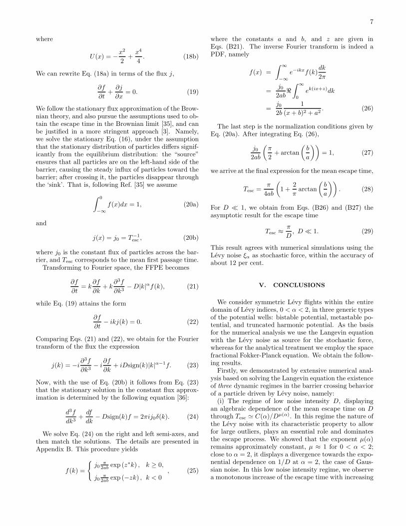
We follow the stationary flux approximation of the Brow-nian theory, and also pursue the assumptions used to ob-tain the escape time in the Brownian limit [35], and canbe justified in a more stringent approach [3]. Namely,we solve the stationary Eq. (16), under the assumptionthat the stationary distribution of particles differs signif-icantly from the equilibrium distribution: the “source”ensures that all particles are on the left-hand side of thebarrier, causing the steady influx of particles toward thebarrier; after crossing it, the particles disappear throughthe ‘sink’. That is, following Ref. [35] we assume

∫ 0

−∞

f(x)dx = 1, (20a)

and

j(x) = j0 = T−1esc , (20b)

where j0 is the constant flux of particles across the bar-rier, and Tesc corresponds to the mean first passage time.

Transforming to Fourier space, the FFPE becomes

∂f

∂t= k

∂f

∂k+ k

∂3f

∂k3−D|k|αf(k), (21)

while Eq. (19) attains the form

∂f

∂t− ikj(k) = 0. (22)

Comparing Eqs. (21) and (22), we obtain for the Fouriertransform of the flux the expression

j(k) = −i∂3f

∂k3− i

∂f

∂k+ iDsign(k)|k|α−1f. (23)

Now, with the use of Eq. (20b) it follows from Eq. (23)that the stationary solution in the constant flux approx-imation is determined by the following equation [36]:

d3f

dk3+df

dk−Dsign(k)f = 2πij0δ(k). (24)

We solve Eq. (24) on the right and left semi-axes, andthen match the solutions. The details are presented inAppendix B. This procedure yields

f(k) =

{

j0π

2ab exp (z∗k) , k ≥ 0,

j0π

2ab exp (−zk) , k < 0, (25)

where the constants a and b, and z are given inEqs. (B21). The inverse Fourier transform is indeed aPDF, namely

f(x) =

∫

∞

−∞

e−ikxf(k)dk

2π

=j02ab

ℜ∫

∞

0

ek(ix+z)dk

=j02b

1

(x+ b)2 + a2. (26)

The last step is the normalization conditions given byEq. (20a). After integrating Eq. (26),

j02ab

(

π

2+ arctan

(

b

a

))

= 1, (27)

we arrive at the final expression for the mean escape time,

Tesc =π

4ab

(

1 +2

πarctan

(

b

a

))

. (28)

For D ≪ 1, we obtain from Eqs. (B26) and (B27) theasymptotic result for the escape time

Tesc ≈π

D, D ≪ 1. (29)

This result agrees with numerical simulations using theLevy noise ξα as stochastic force, within the accuracy ofabout 12 per cent.

V. CONCLUSIONS

We consider symmetric Levy flights within the entiredomain of Levy indices, 0 < α < 2, in three generic typesof the potential wells: bistable potential, metastable po-tential, and truncated harmonic potential. As the basisfor the numerical analysis we use the Langevin equationwith the Levy noise as source for the stochastic force,whereas for the analytical treatment we employ the spacefractional Fokker-Planck equation. We obtain the follow-ing results.

Firstly, we demonstrated by extensive numerical anal-ysis based on solving the Langevin equation the existenceof three dynamic regimes in the barrier crossing behaviorof a particle driven by Levy noise, namely:

(i) The regime of low noise intensity D, displayingan algebraic dependence of the mean escape time on Dthrough Tesc ≃ C(α)/Dµ(α). In this regime the nature ofthe Levy noise with its characteristic property to allowfor large outliers, plays an essential role and dominatesthe escape process. We showed that the exponent µ(α)remains approximately constant, µ ≈ 1 for 0 < α < 2;close to α = 2, it displays a divergence towards the expo-nential dependence on 1/D at α = 2, the case of Gaus-sian noise. In this low noise intensity regime, we observea monotonous increase of the escape time with increasing

8

α (keeping the noise intensity D fixed). The probabilitydensity of escape times decays exponentially.

(ii) The regime of intermediate noise intensity, in whichthe escape time is determined by the central part of prob-ability distribution of the noise. This regime is charac-terized by the following features: The difference betweenthe escape times for different Levy indices significantlydecreases, since in the central part all stable distributionsare very similar to each other, as well as to the Gaussiandistribution. Additionally, there is a non-monotonic de-pendence of the escape time with increasing α. However,the probability densities of escape times still decay expo-nentially.

(iii) The universal regime of high noise intensity, wherethe particle escapes with the first step (or in very fewsteps). The curves denoting the dependence of the escapetime Tesc on noise intensity D collapse onto a single curvefor all values of α (including the Gaussian limit).

Secondly, for the particular Cauchy case, α = 1 wedevelop the kinetic theory of the escape over the barrierin a bistable potential. We start from the space frac-tional Fokker-Planck equation and use the assumption ofa constant flux over the barrier. We find analytically theexpression for the escape time, which at low noise inten-sities produces the result Tesc ≈ π/D. This result agreeswith numerical simulation within the accuracy of about12 per cent.

Acknowledgments

We wish to thank V. Yu. Gonchar and T. Koren fortheir help with the simulations, and M. Lomholt fordiscussions. RM acknowledges partial funding throughthe Natural Sciences and Engineering Research Council(NSERC) of Canada, and the Canada Research Chairsprogramme.

Appendix A: SIMULATIONS DESCRIPTION

In this Appendix, we briefly outline our simulationsstrategy, in particular, how we simulate the white Levynoise ξα (n). The corresponding generator is taken from[37]. We start by calculating the value

X =sin (αγ)

(cos γ)1/α

(

cos ([1 − α]γ)

W

)(1−α)/α

, (A1)

where γ is a random value uniformly distributed on theinterval (−π/2, π/2), W is an independent random vari-able with exponential distribution, and α is the Levyindex, 0 < α ≤ 2.

The proof that the calculated variable X possesses aLevy distribution function goes as follows. Firstly, let0 < α < 1. While γ > 0, the expression for X may be

presented as

X =

(

a(γ)

W

)(1−α)/α

, (A2)

where

a (γ) =

(

sinαγ

cos γ

)α/(1−α)

cos ([1 − α]γ) . (A3)

Then

P (0 ≤ X ≤ x) = P (0 ≤ X ≤ x, γ > 0)

= P

(

0 ≤(

a(γ)

W

)1/α−1

≤ x, γ > 0

)

= P(

W ≥ x−α/(1−α)a(γ), γ > 0)

≡ 1

π

∫ π/2

0

dγ

∫

∞

a(γ)xα/(1−α)

dξe−ξ

=

∫ π/2

0

dγ exp(

−x−α/(1−α)a (γ))

. (A4)

The latter expression, according to Ref. [38] is an integralrepresentation of Levy distribution.

In the case 1 < α ≤ 2 analogous steps pertain, butnow for the quantity P (X ≥ x, γ > 0). When α = 1,the relation for X turns into X = tanγ, that, is knownto be a random value with Cauchy PDF. One does notneed to consider the case γ < 0: it merely correspondsto negative X values.

The numerical simulation of Tesc as function of D isperformed according to the following flowchart:

1. A “particle” is placed at the potential minimum;

2. A value of α is fixed;

3. The discrete-time Langevin equation (8) is iter-ated, until the particle reaches a definite coordi-nate, namely x = 0 for the bistable potential,x = 10 for the metastable potential, and x = ±1for the truncated harmonic potential;

4. The event time t = n∆t is stored;

5. Steps 3 and 4 are executed 10,000 times for eachfixed value of D, and the average escape time cal-culated;

A similar procedure is used to simulate the escape timePDF p(t), apart from taking the average. Explicitly:

1. The “particle” is placed at the potential minimum;

2. Some value of D is fixed;

3. Some value of α is taken;

9

4. The discrete-time Langevin equation (8) is iterated,until the “particle” reaches a definite coordinate,namely x = 0 for the bistable potential, x = 10for the metastable potential, and x = ±1 for thetruncated harmonic potential;

5. The event time t = n∆t is stored;

6. Step 4 is executed 200,000 times for each fixed valueof α, but, this time, the obtained event times arenot averaged, but handled with a simple routine,that builds the PDF;

Each run was repeated and both results compared.Throughout, high reliability was observed.

Appendix B: MATCHING PROCEDURE

In this Appendix, we collect the necessary steps toidentify the constants for the determination of the den-sity f in the barrier crossing for the Cauchy case.

To this end, we solve Eq. (24) on the right and leftsemi-axes, and then match the solutions. For the twodomains, we make the exponential ansatz

f(k) =

{

C1ezk + C2e

z∗k, k > 0;

C3eζk + C4e

ζ∗k, k < 0,(B1)

where

z = −u+ + v+2

+ iu+ − v+

2

√3, (B2)

with

u3+ =

D

2

[

1 +

√

1 +4

27D2

]

, (B3a)

v3+ =

D

2

[

1 −√

1 +4

27D2

]

. (B3b)

Moreover, we define

ζ = −u− + v−2

+ i√

3u− − v−

2, (B4)

with

u3−

=D

2

[

−1 +

√

1 +4

27D2

]

= −v3+, (B5a)

v3−

=D

2

[

−1 −√

1 +4

27D2

]

= −u3+, (B5b)

which implies that

ζ =u+ + v+

2+u+ − v+

2i√

3 , z∗ = −ζ. (B6)

To determine the unknown complex constantsC1, C2, C3, C4 we match the results at k = 0. Thus,

firstly, we require f(k − 0) = f(k + 0), which, usingEq. (B1) yields

C1 + C2 = C3 + C4. (B7)

The second condition is obtained by integration ofEq. (24) over the small region [−ε, ε]:∫ ε

−ε

dkf ′′′ +

∫ ε

−ε

dkf ′ −D

∫ ε

−ε

dksign(k)f = 2πij0. (B8)

In the limit ε→ 0 we recover the condition

f ′′(0+) − f ′′(0−) = 2πij0, (B9)

or, after inserting Eq. (B1) into Eq. (B9),

C1z2 + C2z

∗2 − C3ζ2 − C4ζ

∗2 = 2πij0. (B10)

The third condition is that the PDF is a real function:

f(x) =

∫

∞

0

dk

2πe−ikxf1(k) +

∫ 0

−∞

dk

2πe−ikxf2(k), (B11)

and

f∗(x) =

∫

∞

0

dk

2πeikxf∗

1 (k) +

∫ 0

−∞

dk

2πeikxf∗

2 (k). (B12)

On the other hand, by changing k → −k in Eq. (B11),we find

f(x) =

∫ 0

−∞

dk

2πeikxf1(−k) +

∫

∞

0

dk

2πeikxf2(−k). (B13)

Since f(x) is a real function, we see from Eqs. (B12) and(B13):

f∗

1 (k) = f2(−k), f∗

2 (k) = f1(−k). (B14)

Let us now insert Eq. (B1) into Eqs. (B14). From thefirst equation we have

C∗

1ez∗k + C∗

2ezk = C3e

−ζk + C4e−ζ∗k. (B15)

The second equation gives rise to the same result. Sincez∗ = −ζ (see Eq. (B6)), we have

C∗

1 = C3, C∗

2 = C4. (B16)

Moreover, from Eqs. (B16) and (B7) we see that

(C1 + C2)∗

= C3 + C4 = C1 + C2; (B17)

thus, from Eqs. (B16) and (B17), we obtain the followingrelations:

C1R = C3R, C2R = C4R, (B18a)

C3I = −C1I , C4I = −C2I , (B18b)

C2I = −C1I , C4I = −C3I , (B18c)

C2I = C3I = −C1I = −C4I . (B18d)

10

Therefore, we are actually dealing with 3 constants only,namely, C1R, C2R and CI :

C1 = C1R + iCI , C2 = C2R − iCI , (B19a)

C3 = C1R − iCI , C4 = C2R + iCI . (B19b)

Inserting Eqs. (B19) into Eq. (B10) produces

C1R

(

z2 − ζ2)

+ C2R

(

z∗2 − ζ∗2)

+iCI

(

z2 − z∗2 + ζ2 − ζ∗2)

= 2πij0. (B20)

For convenience, we define

a =u+ + v+

2, b =

√3

2(u+ − v+) . (B21)

Then

z = −a+ ib, ζ = a+ ib; (B22)

such that

z2 − ζ2 = −4iab, (B23a)

z∗2 − ζ∗2 = 4iab, (B23b)

z2 − z∗2 + ζ2 − ζ∗2 = 0. (B23c)

With the use of Eq. (B23) we get from Eq. (B20):

C2R − C1R =πj02ab

. (B24)

Now, combine Eqs. (B19) and (B24), and insert intoEqs. (B1):

f1(k) = (C1R + iCI) ezk +

(

C1R +πj02ab

− iCI

)

ez∗k, k ≥ 0 (B25a)

f2(k) = (C1R − iCI) eζk +

(

C1R +πj02ab

+ iCI

)

eζ∗k, k < 0. (B25b)

We are looking for the stationary (non-equilibrium)distribution; therefore we assume C1R = CI = 0 in orderto retain in Eq. (B25) only those terms, that are propor-tional to the flux j0. This leads us to the result (25).

To calculate the D ≪ 1 limit of the characteristicescape time (29), we obtain the following limiting be-haviours. Thus, from Eqs. (B3) and (B21) we see that

u+ ≈ 1√3

(

1 +

√3D

2

)

, (B26a)

v+ ≈ 1√3

(

−1 +

√3D

2

)

; (B26b)

and

a ≈ D/2, b ≈ 1, (B27a)

arctan

(

b

a

)

≈ arctan

(

2

D

)

≈ π

2. (B27b)

Appendix C: COMPARISON TO ANALYTICRESULTS FROM REF. [26]

In this Appendix, we show that our results are consis-tent with those obtained by Imkeller and Pavlyukevichfrom a different approach to the barrier crossing problemof a particle exposed to Levy stable noise [26].

We recall that in Ref. [26], the authors start from theformula

〈exp (ikLt)〉 = exp (−C(α)t|k|α) , (C1)

with 0 < α < 2, where Lt is the Levy stable processin the Levy-Khintchin representation. The constant C isdefined as

C(α) = 2

∫

∞

0

1 − cos y

y1+αdy =

2Γ(1 − α)

αcos(πα

2

)

(C2)

for α strictly smaller than 2. In Ref. [26], the authorsinvestigate the system driven by the Levy stable processεLt, where ε corresponds to the noise intensity:

〈exp (ikεLt)〉 = exp (−C(α)tεα|k|α) . (C3)

Note that ε is not completely equivalent to our noise in-tensity D. Indeed, in the main body of the paper weinvestigate the system as driven by the Levy stable pro-cess Lt, with

〈exp (ikLt)〉 = exp (−Dt|k|α) . (C4)

Since Lt = εLt, from comparison of Eqs. (C4) and (C3),we see that

D = C(α)εα. (C5)

11

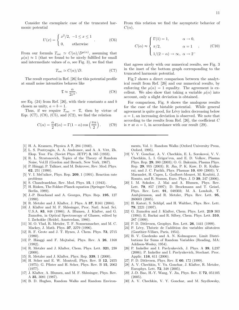
Consider the exemplaric case of the truncated har-monic potential

U(x) =

{

x2/2, −1 ≤ x ≤ 1

0, otherwise. (C6)

From our formula Tesc ≃ C(α)/Dµ(α), assuming thatµ(α) ≈ 1 (that we found to be nicely fulfilled for smalland intermediate values of α, see Fig. 3), we find that

Tesc ≃ C(α)/D. (C7)

The result reported in Ref. [26] for this potential profileat small noise intensities behaves like

T ≈ α

2εα, (C8)

see Eq. (24) from Ref. [26], with their constants a and bchosen as unity, a = b = 1.

Thus, if we require Tesc = T, then by virtue ofEqs. (C7), (C8), (C5), and (C2), we find the relation

C(α) =α

2C(α) = Γ(1 − α) cos

(πα

2

)

. (C9)

From this relation we find the asymptotic behavior ofC(α),

C(α) ≈

Γ(1) = 1, α→ 0,

π/2, α = 1

1/(2 − α) → ∞, α→ 2−

, (C10)

that agrees nicely with our numerical results, see Fig. 3in the inset of the bottom graph corresponding to thetruncated harmonic potential.

Fig.7 shows a direct comparison between the analyt-ical result from Ref. [26] and our numerical results, byenforcing the µ(α) = 1 equality. The agreement is ex-cellent. We also show that taking a variable µ(α) intoaccount, only a slight deviation is obtained.

For comparison, Fig. 8 shows the analogous resultsfor the case of the bistable potential. While generalagreement is quite good, for Levy index decreasing belowα = 1, an increasing deviation is observed. We note thataccording to the results from Ref. [26], the coefficient Cis π at α = 1, in accordance with our result (29).

[1] H. A. Kramers, Physica A 7, 284 (1940).[2] L. S. Pontryagin, A. A. Andronov, and A. A. Vitt, Zh.

Eksp. Teor. Fiz. (Soviet Phys. JETP) 3, 165 (1933).[3] R. L. Stratonovich, Topics of the Theory of Random

Noise, Vol.II (Gordon and Breach, New York, 1967).[4] P. Hanggi, P. Talkner, and M. Bokrovec, Rev. Mod. Phys.

62, 251 (1990).[5] V. I. Mel’nikov, Phys. Rep. 209, 1 (1991). Reaction rate

problems[6] S. Chandrasekhar, Rev. Mod. Phys. 15, 1 (1943).[7] H. Risken, The Fokker-Planck equation (Springer-Verlag,

Berlin, 1989).[8] J.-P. Bouchaud and A. Georges, Phys. Rep. 195, 127

(1990).[9] R. Metzler and J. Klafter, J. Phys. A 37, R161 (2004).

[10] J. Klafter and M. F. Shlesinger, Proc. Natl. Acad. Sci.U.S.A. 83, 848 (1986); A. Blumen, J. Klafter, and G.Zumofen, in Optical Spectroscopy of Glasses, edited byI. Zschokke (Reidel, Amsterdam, 1986).

[11] M. O. Vlad, R. Metzler, T. F. Nonnenmacher, and M. C.Mackey, J. Math. Phys. 37, 2279 (1996).

[12] R. F. Grote and J. T. Hynes, J. Chem. Phys. 73, 2715(1980).

[13] P. Hanggi and F. Mojtabai, Phys. Rev. A 26, 1168(1982).

[14] R. Metzler and J. Klafter, Chem. Phys. Lett. 321, 238(2000).

[15] R. Metzler and J. Klafter, Phys. Rep. 339, 1 (2000).[16] H. Scher and E. W. Montroll, Phys. Rev. B 12, 2455

(1975); G. Pfister and H. Scher, Phys. Rev. B 15, 2062(1977).

[17] J. Klafter, A. Blumen, and M. F. Shlesinger, Phys. Rev.A 35, 3081 (1987).

[18] B. D. Hughes, Random Walks and Random Environ-

ments, Vol. 1: Random Walks (Oxford University Press,Oxford, 1995).

[19] V. Y. Gonchar, A. V. Chechkin, E. L. Sorokovoi, V. V.Chechkin, L. I. Grigor’eva, and E. D. Volkov, PlasmaPhys. Rep. 29, 380 (2003); O. G. Bakunin, Plasma Phys.Rep. 29, 955 (2003); R. Jha, P. K. Kaw, D. R. Kulka-rni, and J. C. Parikh, Phys. Plasmas 10, 699 (2003); Y.Marandet, H. Capes, L. Godbert-Mouret, M. Koubiti, J.Rosato, and R. Stamm, Euro. Phys. J. D 39, 247 (2006).

[20] I. M. Sokolov, J. Mai and A. Blumen, Phys. Rev.Lett. 79, 857 (1997); D. Brockmann and T. Geisel,Phys. Rev. Lett. 91, 048303; M. A. Lomholt, T.Ambjornsson, and R. Metzler, Phys. Rev. Lett. 95,260603 (2005).

[21] H. Katori, S. Schlipf, and H. Walther, Phys. Rev. Lett.79, 2221 (1997).

[22] G. Zumofen and J. Klafter, Chem. Phys. Lett. 219 303(1994); E. Barkai and R. Silbey, Chem. Phys. Lett. 310,287 (1999).

[23] P. D. Ditlevsen, Geophys. Res. Lett. 26, 1441 (1999).[24] P. Levy, Theorie de l’addition des variables aleatoires

(Gauthier-Villars, Paris, 1954).[25] B. V. Gnedenko and A. N. Kolmogorov, Limit Distri-

butions for Sums of Random Variables (Reading, MA:Addison-Wesley, 1954).

[26] P. Imkeller and I. Pavlyukevich, J. Phys. A 39, L237(2006); P. Imkeller and I. Pavlyukevich, Stochast. Proc.Applic. 116, 611 (2006).

[27] P. D. Ditlevsen, Phys. Rev. E 60, 172 (1999).[28] A. V. Chechkin, V. Yu. Gonchar, J. Klafter, R. Metzler,

Europhys. Lett. 72, 348 (2005).[29] J.-D. Bao, H.-Y. Wang, Y. Jia, Phys. Rev. E 72, 051105

(2005).[30] A. V. Chechkin, V. Y. Gonchar, and M. Szydlowsky,

12

Figure 7: Comparison of the coefficients C(α) obtained byusing numerical simulations with the analytical behaviour ofC(α) (full line) derived in Ref. [26], for the truncated harmonicpotential. While the triangles denote our results for µ = 1fixed, the dashed line refers to our results with µ(α), wherewe permit an explicit dependence on α.

Figure 8: Comparison of the coefficients C(α) obtained byusing numerical simulations with the analytical behaviour ofC(α) (full line) derived in Ref. [26], for the bistable potential.

Phys. Plasma 9, 78 (2002); A. V. Chechkin and V. Yu.Gonchar, Zh. Eksp. Teor. Fiz. (JETP) 118, 3, 730 (2000).

[31] The simulation was performed in two ways: first, we usedthe programming language Borland C++ Builder 6 and,second, the symbolic mathematics package Mathemat-ica 5. The step of time was taken equal to 0.01 in Bor-land C++ Builder program and 0.1 in simulation withMathematica. The calculations made on Borland C++Builder and Mathematica gave the same results (the ac-curacy was better than 0.7 percent). It was also provedthat the simulation scheme is independent of the timequantization parameter (the inaccuracy did not exceedan error for the usual scheme of integrating an ordinarydifferential equation of first order by using the method ofrectangles).

[32] We note that in Fig. 2 the values of the noise intensityD for the Gaussian case is larger than the barrier heightand thus Eq. (1) is not valid. Therefore, we here comparethe result of numerical simulation with Eq. (44) fromthe treatise by Malakhov [33], which allows us to avoidthe assumption of the high barrier. The correspondingtheoretical curves are shown in Fig. 2 as bold lines forLevy index α = 2. Obviously, there is excellent agreementbetween analytical solution given in Ref. [33] and thesimulation results.

[33] A. N. Malakhov, Chaos 7, 488 (1997).[34] For the values of α and D shown in Fig. 4 the simula-

tions were performed twice and the results compared. Agood agreement was obained, proving the reliability ofthe simulation.

[35] Yu. L. Klimontovich, Statistical Theory of Open Sys-tems, Vol. I (Kluwer Academic Publishers, Dordrecht,1995).

[36] Note that the Fourier transform of Eq. (20b) reads

j(k) =

Z

∞

−∞

j0eikxdx = 2πj0δ(k). (11)

[37] J. M. Chambers et al., J. Americ. Statist. Assoc. 71, 340(1976).

[38] V. M. Zolotarev, Moscow Mir, p. 187 (1983).