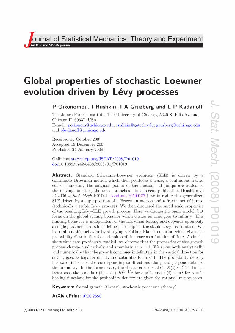
J.Stat.M

ech.(2008)

P01019

ournal of Statistical Mechanics:An IOP and SISSA journalJ Theory and Experiment

Global properties of stochastic Loewnerevolution driven by Levy processes

P Oikonomou, I Rushkin, I A Gruzberg and L P Kadanoff

The James Franck Institute, The University of Chicago, 5640 S. Ellis Avenue,Chicago IL 60637, USAE-mail: poikonom@uchicago.edu, rushkin@gatech.edu, gruzberg@uchicago.eduand l-kadanoff@uchicago.edu

Received 15 October 2007Accepted 19 December 2007Published 24 January 2008

Online at stacks.iop.org/JSTAT/2008/P01019doi:10.1088/1742-5468/2008/01/P01019

Abstract. Standard Schramm–Loewner evolution (SLE) is driven by acontinuous Brownian motion which then produces a trace, a continuous fractalcurve connecting the singular points of the motion. If jumps are added tothe driving function, the trace branches. In a recent publication (Rushkin etal 2006 J. Stat. Mech.P01001 [cond-mat/0509187]) we introduced a generalizedSLE driven by a superposition of a Brownian motion and a fractal set of jumps(technically a stable Levy process). We then discussed the small scale propertiesof the resulting Levy-SLE growth process. Here we discuss the same model, butfocus on the global scaling behavior which ensues as time goes to infinity. Thislimiting behavior is independent of the Brownian forcing and depends upon onlya single parameter, α, which defines the shape of the stable Levy distribution. Welearn about this behavior by studying a Fokker–Planck equation which gives theprobability distribution for end points of the trace as a function of time. As in theshort time case previously studied, we observe that the properties of this growthprocess change qualitatively and singularly at α = 1. We show both analyticallyand numerically that the growth continues indefinitely in the vertical direction forα > 1, goes as log t for α = 1, and saturates for α < 1. The probability densityhas two different scales corresponding to directions along and perpendicular tothe boundary. In the former case, the characteristic scale is X(t) ∼ t1/α. In thelatter case the scale is Y (t) ∼ A + Bt1−1/α for α �= 1, and Y (t) ∼ ln t for α = 1.Scaling functions for the probability density are given for various limiting cases.

Keywords: fractal growth (theory), stochastic processes (theory)

ArXiv ePrint: 0710.2680

c©2008 IOP Publishing Ltd and SISSA 1742-5468/08/P01019+27$30.00

J.Stat.M

ech.(2008)

P01019

Global properties of stochastic Loewner evolution driven by Levy processes

Contents

1. Introduction 2

2. The model and the results, old and new 3

3. Derivation of the Fokker–Planck equation 5

4. Qualitative description, distance scales 10

5. Solving the FPE 115.1. Results for α > 1 . . . . . . . . . . . . . . . . . . . . . . . . . . . . . . . . 145.2. Results for α = 1 . . . . . . . . . . . . . . . . . . . . . . . . . . . . . . . . 175.3. Results for α < 1 . . . . . . . . . . . . . . . . . . . . . . . . . . . . . . . . 20

6. Conclusions 23

Acknowledgments 24

Appendix A. Numerical calculations 24

Appendix B. Asymptotics for K(λ, y) 25

References 27

1. Introduction

The study of random conformally invariant clusters that appear at critical points in two-dimensional statistical mechanics models has been made rigorous with the invention ofthe so-called Schramm–Loewner evolution (SLE) [2]. SLE refers to a continuous familyof evolving conformal maps that specify the shape of a part of a critical cluster boundary.By now SLE has been justly recognized as a major breakthrough, and there are severalreview papers and one monograph devoted to this beautiful subject, see [3]–[10].

SLE describes a curve, called trace, growing with time from a boundary in a two-dimensional domain which is usually chosen to be the upper half plane. SLE is based onthe Loewner equation in which the shape of the growing curve is determined by a functionof time ξ(t) which in SLE is taken to be a scaled Brownian motion. Such a choice of thedriving function produces continuous stochastic, fractal and conformally invariant curves,—the kind that appears as the scaling limit of various interfaces in many two-dimensionalcritical lattice models and growth processes of statistical physics. Well-known examplesinclude boundaries of the Fortuin–Kastelyn clusters in the critical q-state Potts model,loops in the O(n) model, self-avoiding and loop-erased random walks.

In [1] we generalized SLE to a broader class for which ξ(t) is a Markov process withdiscontinuities. More specifically, we have studied the Loewner evolution driven by alinear combination of a scaled Brownian motion and a symmetric stable Levy process.The growing curve then exhibits branching. This generalized process might be usefulto describe many tree-like growth processes, such as branching polymers and variousbranching growth processes which evolve in time.

doi:10.1088/1742-5468/2008/01/P01019 2

J.Stat.M

ech.(2008)

P01019

Global properties of stochastic Loewner evolution driven by Levy processes

Such generalized SLEs driven by Levy processes (Levy-SLE for short) have also beenof interest to mathematics community. Our results [1] on various phase transitions inLevy-SLE have been put on rigorous basis in [11], and further properties have beenstudied in [12, 13]. The interest of mathematicians in these Levy-SLE processes ispartially motivated by the suggestion [13, 14] that they may produce fractal objects withlarge values of multifractal exponents for harmonic measure. Harmonic measure can bethought of as the charge distribution on the boundary of a conducting cluster. On fractalboundaries such a distribution is a multifractal, and in the case of critical clusters (whoseboundaries are SLE curves) the full spectrum of multifractal exponents has been obtainedanalytically, see [14]–[18] for various derivations and discussion.

While our previous paper [1] focused on local properties of Levy-SLE, here we studythe global behavior of the growth in the upper half plain. The present paper is structuredas follows. In section 2 we define our model and briefly state our previous results on phasetransitions in the local behavior of the model. We also present our new results on theglobal behavior of Levy-SLE. In section 3 we derive the Fokker–Planck equation governingthe evolution of the probability distribution for the tip of the Levy-SLE. The equationis our main tool for analysis of the long time global behavior of the growth. We givea qualitative description of the growth and explain the approximations that go into thesolution of the Fokker–Planck equation in section 4. Actual solution of the Fokker–Planckequation and comparison with results from numerically calculated trajectories is given insection 5. We conclude in section 6. Some technical details are presented in appendices.

2. The model and the results, old and new

Loewner evolution is a family of conformal maps that appears as the solution of theLoewner differential equation (see, for example, [3] for details)

∂tgt(z) =2

gt(z) − ξ(t), g0(z) = z, (1)

valid at any point z in the upper half plane until (and if) this point becomes singular atsome (possibly infinite) time τz : ξ(τz) = gτz(z). The set of all singularities is called thehull and the point at which the hull grows is called the tip. The tip γ(t) is defined via itsimage ξ(t) = gt(γ(t)). More formally,

γ(t) = limw→ξ(t)

g−1t (w), (2)

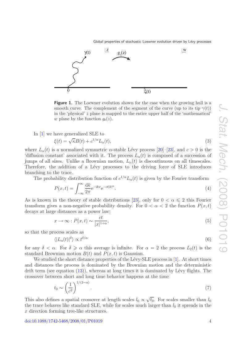
where the limit is taken in the upper half plane. The trace is the path left behind by thetip (the existence of the trace in the setting of this paper has been shown in [12]). Theshape of the growing trace (and the hull) is completely determined by the driving functionξ(t). At any time the function gt(z) conformally maps the exterior of the growing hull tothe upper half plane, see figure 1. We refer to the z plane where the growth occurs as ‘thephysical plane’, and to the w plane as ‘the mathematical plane’.

Naturally, if ξ(t) is a stochastic process the shape of the growing trace is alsostochastic. The growth process is then a stochastic (Schramm–) Loewner evolution (SLE).The standard SLE has a driving function ξ(t) =

√κB(t), where B(t) is a normalized

Brownian motion and κ > 0 is the diffusion constant. Many important properties of thisprocess have been established in [19].

doi:10.1088/1742-5468/2008/01/P01019 3

J.Stat.M

ech.(2008)

P01019

Global properties of stochastic Loewner evolution driven by Levy processes

Figure 1. The Loewner evolution shown for the case when the growing hull is asmooth curve. The complement of the segment of the curve (up to its tip γ(t))in the ‘physical’ z plane is mapped to the entire upper half of the ‘mathematical’w plane by the function gt(z).

In [1] we have generalized SLE to

ξ(t) =√

κB(t) + c1/αLα(t), (3)

where Lα(t) is a normalized symmetric α-stable Levy process [20]–[23], and c > 0 is the‘diffusion constant’ associated with it. The process Lα(t) is composed of a succession ofjumps of all sizes. Unlike a Brownian motion, Lα(t) is discontinuous on all timescales.Therefore, the addition of a Levy processes to the driving force of SLE introducesbranching to the trace.

The probability distribution function of c1/αLα(t) is given by the Fourier transform

P (x, t) =

∫ ∞

−∞

dk

2πe−ikxe−ct|k|α. (4)

As is known in the theory of stable distributions [23], only for 0 < α � 2 this Fouriertransform gives a non-negative probability density. For 0 < α < 2 the function P (x, t)decays at large distances as a power law:

x → ∞ : P (x, t) ∼ ct

|x|1+α, (5)

so that the process scales as

〈|Lα(t)|δ〉 ∝ tδ/α (6)

for any δ < α. For δ � α this average is infinite. For α = 2 the process L2(t) is thestandard Brownian motion B(t) and P (x, t) is Gaussian.

We studied the short distance properties of the Levy-SLE process in [1]. At short timesand distances the process is dominated by the Brownian motion and the deterministicdrift term (see equation (13)), whereas at long times it is dominated by Levy flights. Thecrossover between short and long time behavior happens at the time

t0 ∼(

1

c2

)1/(2−α)

. (7)

This also defines a spatial crossover at length scales l0 ∝√

t0. For scales smaller than l0the trace behaves like standard SLE, while for scales much larger than l0 it spreads in thex direction forming tree-like structures.

doi:10.1088/1742-5468/2008/01/P01019 4

J.Stat.M

ech.(2008)

P01019

Global properties of stochastic Loewner evolution driven by Levy processes

In our previous paper [1], using both analytic and numerical considerations, wedetermined the probability that a point on the x axis is swallowed by the trace. Thetrace shows a qualitative change in its small distance, small time behavior as κ and αeach pass though critical values, respectively at four and one. The transition at κ = 4 isquite analogous to the known transition of standard SLE [19]. For the new transition atα = 1, the trace forms isolated trees when α < 1 or a dense forest when α > 1.

The latter phase transition at α = 1 was recently studied rigorously in [11] whichexpanded the implications of the phase transition to the whole plane at the limit t → ∞.For κ > 4 a point in the upper half plane is swallowed almost surely for α > 1, while itis swallowed with probability smaller than one for α < 1. For κ < 4 and 0 < α < 2 theswallowed points on the plane form a set of measure zero.

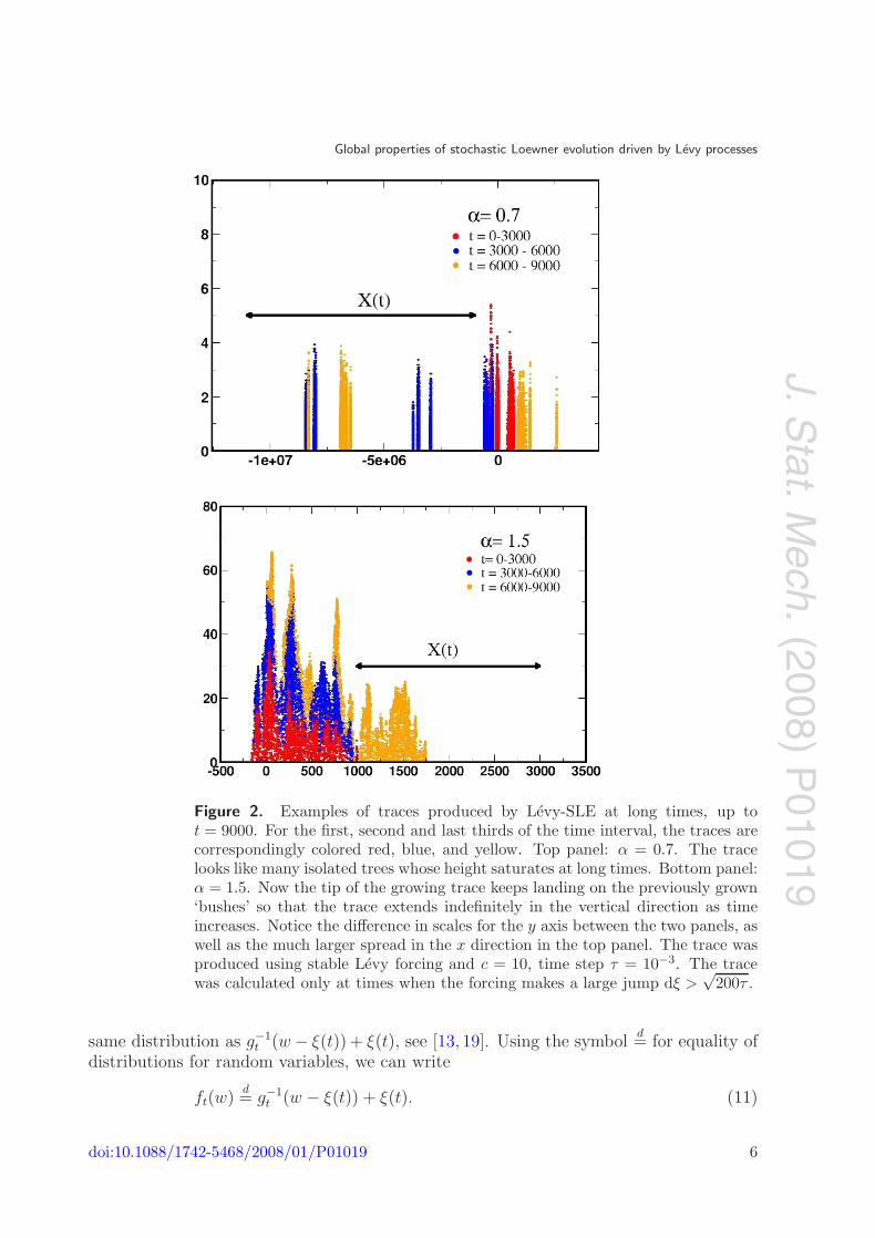
The large scale implications of the α = 1 transition can be seen in figure 2 whichshows the shape of the trace at long times. For α < 1 the stochastic evolution producesisolated tree-like structures which are limited in height. For α > 1 the evolution producesan ‘underbrush’ in which structures pile on one another and thereby continue to increasetheir height.

In the rest of the paper we establish the following. The growth at long times ischaracterized by two very different length scales X(t) and Y (t) (with X(t) Y (t)) whichcan be thought of as the typical size of the growing hull in the x and y directions. Morespecifically, we find that

X(t) ∼ t1/α, 0 < α < 2, (8)

Y (t) ∼{

A + Bt1−1/α, α �= 1,

ln t, α = 1.(9)

(The constants A and B depend upon α.) These scales enter the scaling form of the jointprobability distribution ρ(x, y, t) for the real and imaginary parts of the tip γ(t) of theLevy-SLE, for which we give explicit results in various limiting cases in section 5, wherewe also compare analytical results with extensive numerical simulations.

3. Derivation of the Fokker–Planck equation

We are interested in characterizing the probability distribution for the point γ(t) at thetip of the trace in the ensemble provided by different realizations of the SLE stochasticprocess. Equation (2) implies then that we should study the inverse map g−1

t . However,this is rather difficult, since the map g−1

t satisfies a partial differential equation instead ofan ODE. There is a way out which is rather well known and has been successfully usedbefore [13, 14, 19]. It happens that one needs to consider the backward time evolution:

∂tft(w) = − 2

ft(w) − ξ(t), f0(w) = w. (10)

The relation of the original Loewner evolution (1) and the backward one (10) in thestochastic setting is as follows. If ξ(t) is a symmetric (in time) process with independentidentically distributed increments, which is the case for a Levy process, then it is easy toshow that for any fixed time t the solution ft(w) of the backward equation (10) has the

doi:10.1088/1742-5468/2008/01/P01019 5

J.Stat.M

ech.(2008)

P01019

Global properties of stochastic Loewner evolution driven by Levy processes

Figure 2. Examples of traces produced by Levy-SLE at long times, up tot = 9000. For the first, second and last thirds of the time interval, the traces arecorrespondingly colored red, blue, and yellow. Top panel: α = 0.7. The tracelooks like many isolated trees whose height saturates at long times. Bottom panel:α = 1.5. Now the tip of the growing trace keeps landing on the previously grown‘bushes’ so that the trace extends indefinitely in the vertical direction as timeincreases. Notice the difference in scales for the y axis between the two panels, aswell as the much larger spread in the x direction in the top panel. The trace wasproduced using stable Levy forcing and c = 10, time step τ = 10−3. The tracewas calculated only at times when the forcing makes a large jump dξ >

√200τ .

same distribution as g−1t (w − ξ(t)) + ξ(t), see [13, 19]. Using the symbol

d= for equality of

distributions for random variables, we can write

ft(w)d= g−1

t (w − ξ(t)) + ξ(t). (11)

doi:10.1088/1742-5468/2008/01/P01019 6

J.Stat.M

ech.(2008)

P01019

Global properties of stochastic Loewner evolution driven by Levy processes

It is useful to introduce a shifted conformal map

ht(z) = gt(z) − ξ(t), (12)

for which the Loewner equation acquires the Langevin-like form:

∂tht(z) =2

ht(z)− ∂tξ(t), h0(z) = z, (13)

assuming that ξ vanishes at t = 0. The first term is a deterministic drift and the second—arandom noise. The tip γ(t) is now mapped to zero, and this can be taken as the definitionof the tip. More formally,

γ(t) = limw→0

h−1t (w), (14)

where the limit is taken in the upper half plane.In terms of the shifted map the equality of distributions (11) can be written as

ft(w) − ξ(t)d= h−1

t (w). (15)

The left-hand side zt ≡ ft(w) − ξ(t) of this equation satisfies the Langevin-like equation

∂tzt = − 2

zt

− ∂tξ(t), z0 = w, (16)

and in particular, if we set w = 0 in this equation, the resulting stochastic dynamicsshould be the same as that of the tip of the trace γ(t).

Before we convert the Langevin-like equation (16) to our main analytical tool, thecorresponding Fokker–Planck equation, let us review again the correspondence betweenthe forward and backward flows and illustrate it with figures. Equation (13) describesa flow in which wt = ht(z) follows a trajectory of a particle in the w plane, z being itsinitial position. Separating the real and imaginary parts of wt = ut + ivt, we get a systemof coupled equations

∂tut =2ut

u2t + v2

t

− ∂tξ(t), u0 = x,

∂tvt = − 2vt

u2t + v2

t

, v0 = y,(17)

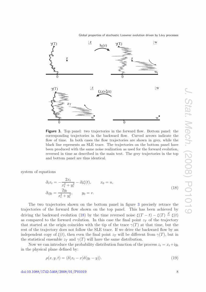
describing such a trajectory. As in many modern versions of dynamics, all initial conditionsand hence all trajectories are considered at the same time, forming an ensemble. Two suchtrajectories are presented on the top panel in figure 3. For a generic initial point z thetrajectory wt goes to infinity in the horizontal u direction, while the vertical coordinatevt monotonously decreases. However, if the initial point happens to be a point γ(T ) onthe SLE trace, the forward trajectory hits the origin in the mathematical plane exactlyat time T .

Conversely, we can fix a point w in the mathematical plane and follow the motion ofits image zt under the map ft(w) − ξ(t) in the physical plane, with the initial conditionz0 = w. In components zt = xt + iyt, the trajectories of this backward flow satisfy the

doi:10.1088/1742-5468/2008/01/P01019 7

J.Stat.M

ech.(2008)

P01019

Global properties of stochastic Loewner evolution driven by Levy processes

Figure 3. Top panel: two trajectories in the forward flow. Bottom panel: thecorresponding trajectories in the backward flow. Curved arrows indicate theflow of time. In both cases the flow trajectories are shown in grey, while theblack line represents an SLE trace. The trajectories on the bottom panel havebeen produced with the same noise realization as used for the forward evolution,reversed in time as described in the main text. The grey trajectories in the topand bottom panel are thus identical.

system of equations

∂txt = − 2xt

x2t + y2

t

− ∂tξ(t), x0 = u,

∂tyt =2yt

x2t + y2

t

, y0 = v.(18)

The two trajectories shown on the bottom panel in figure 3 precisely retrace thetrajectories of the forward flow shown on the top panel. This has been achieved by

driving the backward evolution (18) by the time reversed noise ξ(T − t) − ξ(T )d= ξ(t)

as compared to the forward evolution. In this case the final point zT of the trajectorythat started at the origin coincides with the tip of the trace γ(T ) at that time, but therest of the trajectory does not follow the SLE trace. If we drive the backward flow by anindependent copy of ξ(t), then even the final point zT will be different from γ(T ), but inthe statistical ensemble zT and γ(T ) will have the same distribution.

Now we can introduce the probability distribution function of the process zt = xt +iyt

in the physical plane defined by:

ρ(x, y, t) = 〈δ(xt − x)δ(yt − y)〉. (19)

doi:10.1088/1742-5468/2008/01/P01019 8

J.Stat.M

ech.(2008)

P01019

Global properties of stochastic Loewner evolution driven by Levy processes

From equations (3) and (18) it follows immediately that ρ(x, y, t) satisfies the following(generalized) Fokker–Planck equation:

∂tρ(x, y, t) =

[κ

2∂2

x + c|∂x|α + ∂x2x

x2 + y2− ∂y

2y

x2 + y2

]ρ(x, y, t). (20)

Here |∂x|α (sometimes also written as (−Δ)α/2) is the Riesz fractional derivative, whichis a singular integral operator whose action is easiest to describe in the Fourier space: iff(k) is the Fourier transform of a function f(x), then the Fourier transform of |∂x|αf(x)

is |k|αf(k).As we have discussed, at long times the growth is dominated by the stable process in

the driving function (3), and we can set κ = 0. So our main analytical tool is the followingFokker–Planck equation:

∂tρ(x, y, t) =

[c|∂x|α + ∂x

2x

x2 + y2− ∂y

2y

x2 + y2

]ρ(x, y, t). (21)

Let us discuss the boundary and initial conditions for this equation. The initialcondition for the Fokker–Planck equation (21) depends on the initial conditions x0 = u,y0 = v in the stochastic equations (18). For the distribution of the SLE tip γ(t) theappropriate initial conditions are x0 = 0, y0 = ε, where ε is an infinitesimal positivenumber. For the exact Fokker–Planck equation (20) this translates into the initialcondition

ρ(x, y, 0) = δ(x)δ(y − ε). (22)

However, for the approximate equation (21) the situation is more subtle. The crossovertime t0 = O(1). For t < t0 the drift in the x direction (towards x = 0) dominates overthe Levy term. For t > t0 the opposite is true. A simple picture is then that before t0 theinitial δ function is advected by the drift velocity 2/y in the y direction. By the time t0it becomes

ρ0(x, y) ≡ ρ(x, y, t0) = δ(x)δ(y − y0), y0 = 2t1/20 ∼ c−1/(2−α). (23)

This is the initial value that we shall assume for our problem. In the following sectionswe will mostly use the notation ρ0(x, y), using the explicit expression when necessary.

Let us comment that if we tried to be more careful and included the effects of theBrownian forcing before the crossover time t0, then the distribution at time t0 would notonly be advected to y0 but would also broaden to a Gaussian with variance κt0. Thisrefinement would not change any arguments in the later sections, since all we need thereis that the Fourier transform in x of the initial distribution is broader than e−ct|kα| forlong times, see the discussion preceding equation (36). This is a good approximation forboth the initial distribution (23) or its Gaussian variant for sufficiently long times, andbecomes better and better as time increases.

As for the boundary conditions at y = 0, we have no need to be very explicit aboutthem, since ρ(x, y, 0) vanishes for y < y0, and our equations of motion (18) represent asituation in which yt continually increases as t increases, so that ρ(x, y, t) will also vanishfor y < y0 at all times t > 0.

doi:10.1088/1742-5468/2008/01/P01019 9

J.Stat.M

ech.(2008)

P01019

Global properties of stochastic Loewner evolution driven by Levy processes

4. Qualitative description, distance scales

In this section we analyze in qualitative terms the long time limit of the evolution of thetip γ(t), by looking at the consequences of equations (18). According to the discussion inthe previous section, Re γ(t) and Im γ(t) have the same joint distribution as xt and yt.

For small times, up to the crossover time t0, the drift term in the Langevin equationdominates over the Levy noise. Therefore, both xt and yt, and ξ(t) as well, grow as

√t.

For larger times, t t0, there are two different characteristic length scales, X(t) and Y (t).In this regime the forcing ξ(t) is dominated by the Levy process Lα(t). The probability fora total motion X(t) over a time t for this process is described by equation (4). Typicallythe motion is dominated by a single long jump, and the jump has an order of magnitude

X(t) ∼ (ct)1/α. (24)

(This can be understood as rescaled fractional moments 〈|Lα(t)|δ〉1/δ, see equation (6).)Since the typical jumps of ξ(t) become arbitrarily large at long times, xt also becomeslarge, and therefore, the drift term in the first equation of (18) becomes negligible. In thislimit, xt behaves like the driving force, and we find

t → ∞ : |xt| ∼ X(t) ∼ (ct)1/α. (25)

The Loewner evolution with Levy flights produces, in general, a forest of (sparse or dense)branching trees, growing form the real axis. The above relation then tells us how the forestspreads along the real axis with time. This distance is marked out on the plots of treesshown in figure 2.

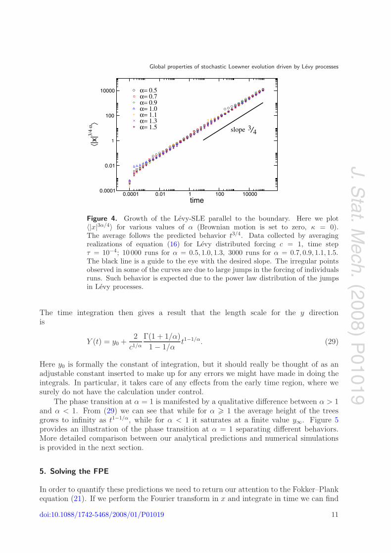
Numerical implementation of the Langevin equation (16), details of which arepresented in appendix A, confirms these qualitative arguments. Figure 4 compares theestimate of equation (25) with numerical calculations of the trace via simulations ofequation (16). The agreement is excellent.

Next we turn to a typical distance Y (t) in the y coordinate. Figure 2 clearly showsthat this characteristic distance is much smaller than X(t). We understand this as follows.If xt were zero, the second equation in (18) would give yt ∼ t1/2. Clearly, any non-zero xt

only slows down the growth of yt. We then conclude that yt, and therefore the height of thetrees produced by the SLE process cannot grow with time faster than t1/2. Since α < 2, itmeans that Im γ(t) always grows slower than Re γ(t) and they become widely separatedat long times. Our major result is that the growing trees spread faster horizontally thanthey grow vertically. Hence, we have

Y (t) � X(t). (26)

An estimate of the scaling of Y (t) can be obtained from the second equation in (18)where we replace xt by the Levy process and average over it using the probabilitydistribution (4). This gives a typical behavior of yt:

∂tyt ≈∫ ∞

−∞dx

2yt

y2t + x2

P (x, t) =

∫ ∞

−∞dk e−yt|k|−c|k|αt. (27)

To estimate the k integral we can drop the term yt|k| in the exponent, since this quantityis of order Y (t)/X(t) � 1. Thus we get

∂tyt ≈2Γ (1 + 1/α)

c1/αt−1/α. (28)

doi:10.1088/1742-5468/2008/01/P01019 10

J.Stat.M

ech.(2008)

P01019

Global properties of stochastic Loewner evolution driven by Levy processes

0.0001 0.01 1 100 10000time

0.0001

0.01

1

100

10000⟨|x

|3/4

α ⟩α= 0.5α= 0.7α= 0.9α= 1.0α= 1.1α= 1.3α= 1.5 3/4slope

Figure 4. Growth of the Levy-SLE parallel to the boundary. Here we plot〈|x|3α/4〉 for various values of α (Brownian motion is set to zero, κ = 0).The average follows the predicted behavior t3/4. Data collected by averagingrealizations of equation (16) for Levy distributed forcing c = 1, time stepτ = 10−4; 10 000 runs for α = 0.5, 1.0, 1.3, 3000 runs for α = 0.7, 0.9, 1.1, 1.5.The black line is a guide to the eye with the desired slope. The irregular pointsobserved in some of the curves are due to large jumps in the forcing of individualsruns. Such behavior is expected due to the power law distribution of the jumpsin Levy processes.

The time integration then gives a result that the length scale for the y directionis

Y (t) = y0 +2

c1/α

Γ(1 + 1/α)

1 − 1/αt1−1/α. (29)

Here y0 is formally the constant of integration, but it should really be thought of as anadjustable constant inserted to make up for any errors we might have made in doing theintegrals. In particular, it takes care of any effects from the early time region, where wesurely do not have the calculation under control.

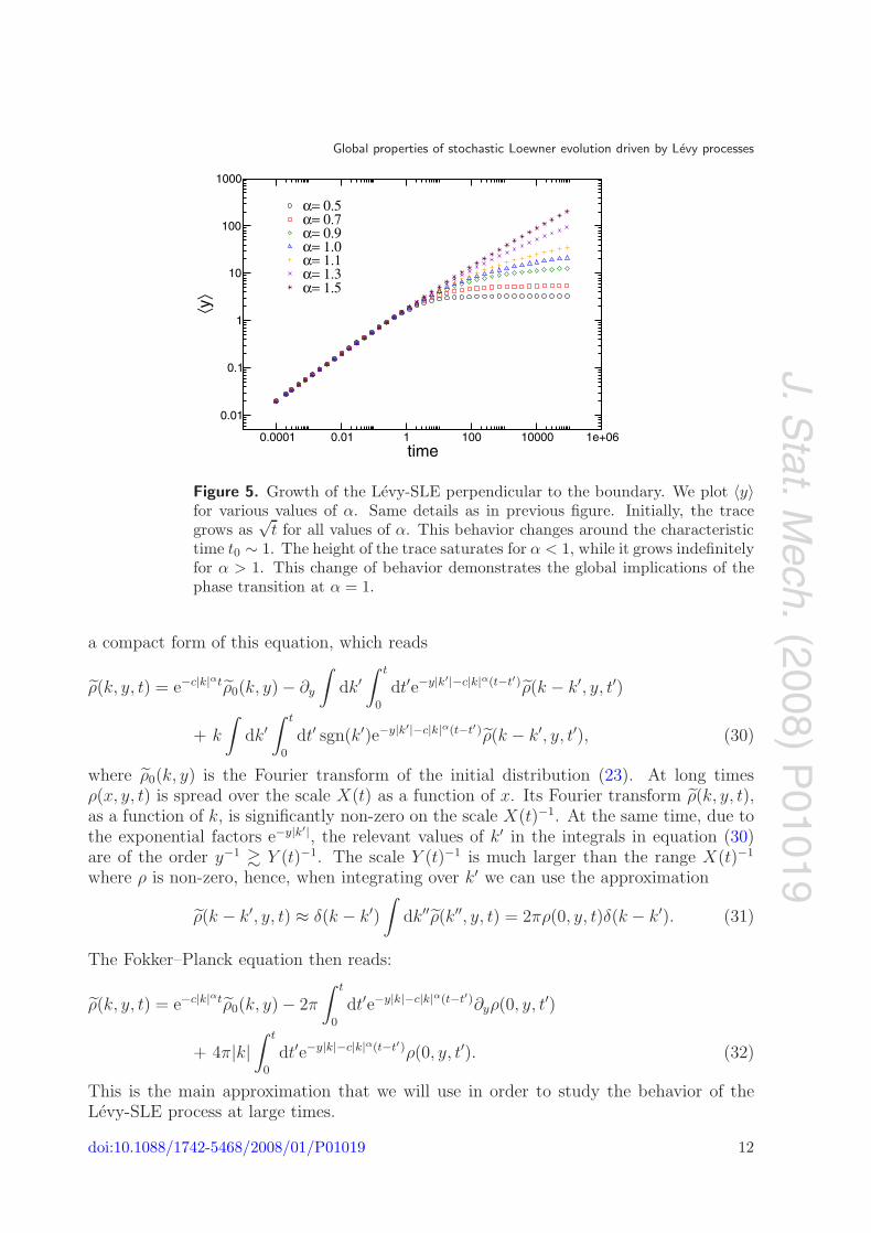
The phase transition at α = 1 is manifested by a qualitative difference between α > 1and α < 1. From (29) we can see that while for α � 1 the average height of the treesgrows to infinity as t1−1/α, while for α < 1 it saturates at a finite value y∞. Figure 5provides an illustration of the phase transition at α = 1 separating different behaviors.More detailed comparison between our analytical predictions and numerical simulationsis provided in the next section.

5. Solving the FPE

In order to quantify these predictions we need to return our attention to the Fokker–Plankequation (21). If we perform the Fourier transform in x and integrate in time we can find

doi:10.1088/1742-5468/2008/01/P01019 11

J.Stat.M

ech.(2008)

P01019

Global properties of stochastic Loewner evolution driven by Levy processes

0.0001 0.01 1 100 10000 1e+06time

0.01

0.1

1

10

100

1000

⟨y⟩

α= 0.5α= 0.7α= 0.9α= 1.0α= 1.1α= 1.3α= 1.5

Figure 5. Growth of the Levy-SLE perpendicular to the boundary. We plot 〈y〉for various values of α. Same details as in previous figure. Initially, the tracegrows as

√t for all values of α. This behavior changes around the characteristic

time t0 ∼ 1. The height of the trace saturates for α < 1, while it grows indefinitelyfor α > 1. This change of behavior demonstrates the global implications of thephase transition at α = 1.

a compact form of this equation, which reads

ρ(k, y, t) = e−c|k|αtρ0(k, y) − ∂y

∫dk′

∫ t

0

dt′e−y|k′|−c|k|α(t−t′)ρ(k − k′, y, t′)

+ k

∫dk′

∫ t

0

dt′ sgn(k′)e−y|k′|−c|k|α(t−t′)ρ(k − k′, y, t′), (30)

where ρ0(k, y) is the Fourier transform of the initial distribution (23). At long timesρ(x, y, t) is spread over the scale X(t) as a function of x. Its Fourier transform ρ(k, y, t),as a function of k, is significantly non-zero on the scale X(t)−1. At the same time, due tothe exponential factors e−y|k′|, the relevant values of k′ in the integrals in equation (30)are of the order y−1 � Y (t)−1. The scale Y (t)−1 is much larger than the range X(t)−1

where ρ is non-zero, hence, when integrating over k′ we can use the approximation

ρ(k − k′, y, t) ≈ δ(k − k′)

∫dk′′ρ(k′′, y, t) = 2πρ(0, y, t)δ(k − k′). (31)

The Fokker–Planck equation then reads:

ρ(k, y, t) = e−c|k|αtρ0(k, y) − 2π

∫ t

0

dt′e−y|k|−c|k|α(t−t′)∂yρ(0, y, t′)

+ 4π|k|∫ t

0

dt′e−y|k|−c|k|α(t−t′)ρ(0, y, t′). (32)

This is the main approximation that we will use in order to study the behavior of theLevy-SLE process at large times.

doi:10.1088/1742-5468/2008/01/P01019 12

J.Stat.M

ech.(2008)

P01019

Global properties of stochastic Loewner evolution driven by Levy processes

Notice here that the distribution function ρ, for every x and t, depends only on theinitial condition ρ0 and the history of the distribution at x = 0 for earlier times t′ < t.Therefore, in order to study the probability density function described by the Fokker–Planck equation, we first need to calculate the behavior of this distribution for small x,that is ρ(0, y, t). Then, by substituting in equation (32), we can in principle estimate thefull distribution. However, in this paper we are mostly interested in the way this processgrows in the y direction. Hence, we will first find ρ(0, y, t) which characterizes the growthnear x = 0, and then obtain the distribution

p(y, t) ≡∫ ∞

−∞dx ρ(x, y, t) = ρ(0, y, t) (33)

of y’s integrated over all x by setting k = 0 in (32):

p(y, t) = p0(y) − 2π

∫ t

0

dt′ ∂yρ(0, y, t′). (34)

This equation immediately leads to the average 〈y〉, which is understood as the averageover all x:

〈y〉 = y0 + 2π

∫ t

0

dt′∫ ∞

0

dy ρ(0, y, t′). (35)

Therefore, the distribution and its mean in equations (34) and (35) depend only on thebehavior at x = 0 at times t′ < t. This is a direct implication of equation (32) and ourmain approximation (31).

Let us emphasize again that our approximation works in the long time limit. We willassume that we can use approximate expressions in time integrals for all t > t0. Thus,we will treat all time integrals

∫ t

0as

∫ t

t0+ correction. The corrections come from short

times, and we cannot extract them from our analysis. They all will be hidden in the termsdependent on the lower limit t0 of the time integrals. In several cases the lower cut-off att0 is necessary to avoid spurious divergencies.

Let us now consider ρ(0, y, t). A closed equation for this quantity results fromintegrating equation (32) over k. To do this we observe that in the first term (the initialvalue at t = 0) for the relevant values of k the function ρ0(k, y) is much broader in k thane−c|k|αt at long times. Hence, in the integral over k we can replace ρ0(k, y) by its value atk = 0. Then it follows that

ρ(0, y, t) =ρ0(0, y)

2πX(t)−

∫ t

0

dt′∂yρ(0, y, t′)

X(t − t′, y)− 2

∫ t

0

dt′ρ(0, y, t′)∂y1

X(t − t′, y), (36)

where the scale X(t, y) is defined as

1

X(t, y)=

∫ ∞

−∞dk e−c|k|αt−y|k|, (37)

and

X(t) = X(t, y = 0) =c1/α

2Γ (1 + 1/α)t1/α. (38)

doi:10.1088/1742-5468/2008/01/P01019 13

J.Stat.M

ech.(2008)

P01019

Global properties of stochastic Loewner evolution driven by Levy processes

Equation (36) is easily solved after performing the Laplace transformation in time t.For the transform

ρ(0, y, λ) =

∫ ∞

0

dt e−λtρ(0, y, t) (39)

we obtain an ordinary differential equation

∂yρ(0, y, λ) +1 + 2∂yK(λ, y)

K(λ, y)ρ(0, y, λ) =

K(λ)

2πK(λ, y)ρ0(0, y), (40)

where

K(λ, y) =

∫ ∞

0

dte−λt

X(t, y)=

∫ ∞

−∞dk

e−y|k|

λ + c|k|α , (41)

and K(λ) = K(λ, 0). Using the initial condition ρ0(0, y) = δ(y − y0), the straightforwardsolution of equation (40) is

ρ(0, y, λ) =K(λ)

2π

K(λ, y0)

K2(λ, y)exp

(−

∫ y

y0

dy′

K(λ, y′)

). (42)

The inverse Laplace transform of this solution gives ρ(0, y, t).Notice that (42) is valid only for y > y0. Since our approximations only work at

long times, we expect our solution to give good results for y y0. The approximationswill usually result in the necessity to introduce a fitting parameter (called ‘correction’in the discussion after equation (35)) in the time evolution of averages for the process.Moreover, there is an upper cut-off that stems from the Langevin equation and the factthat y cannot grow faster than t1/2 (see previous section). Since we used this fact whilemaking the approximations that lead to equation (32), the range of validity of our solutionis y0 � y � t1/2.

In the following we will analyze the properties of the distributions ρ(0, y, t) and p(y, t)in three separate cases α > 1, α = 1 and α < 1. For each case we will repeat the followingsteps: first we calculate ρ(0, y, t) from equation (42), then, by substituting this solutioninto equation (34), we will calculate the average height 〈y〉 and the distribution p(y, t).In these calculations we need approximate expressions for the function K(λ, y). Theseexpressions are derived in appendix B.

5.1. Results for α > 1

In this case we can use the approximation (B.12) from appendix B for K(λ) and K(λ, y).Equation (42) then gives

ρ(0, y, λ) ≈ 1

2πexp

(− 1

Aλ1−1/αy

), A =

2π

αc1/α sin(π/α). (43)

To calculate the time dependence of the distribution we take the inverse Laplace transform:

ρ(0, y, t) ≈ 1

2πt

∫ a+∞

a−i∞

dλ

2πieλt−λ1−1/αy/A. (44)

As usual, the integration contour in the last equation goes along a vertical line Reλ = a,where a should be greater than the real part of any singularity of the integrand. Changing

doi:10.1088/1742-5468/2008/01/P01019 14

J.Stat.M

ech.(2008)

P01019

Global properties of stochastic Loewner evolution driven by Levy processes

the integration variable to λt we obtain that answer which, apart from the overall prefactor1/t, has acquired the form of a scaling function:

ρ(0, y, t) ≈ 1

2πtF (y), y ≡ y

Y (t), Y (t) =

2

c1/α

π

α sin(π/α)t1−1/α, (45)

F (y) =

∫dλ

2πieλ−λ1−1/α y. (46)

Since the scaling function F (y) depends only on the combination yt−1+1/α, its derivativeswith respect to y and t are related:

∂yF (y) = − α

α − 1

t

y∂tF (y). (47)

The integrand in equation (46) contains a branch cut which we choose to run alongthe negative real axis. The integration contour can be deformed to go from −∞ to 0along the lower side of the cut, and then from 0 to −∞ along the upper side. This leadsto the final answer for the scaling function F (y):

F (y) =1

π

∫ ∞

0

dλ e−λ−| cos(π/α)|λ1−1/α y sin

(sin

π

αλ1−1/αy

). (48)

The overall prefactor 1/t in ρ(0, y, t) can be understood as follows. The distributionρ(x, y, t) at long times spreads in the x direction up to scale X(t), and in the y direction upto scale Y (t). The total area ‘covered’ by the distribution scales with time as X(t)Y (t) ∝ t.Therefore, at the particular value x = 0 the density ρ(0, y, t) decays with time as 1/t.However, if we are looking at the distribution of the y coordinate for x = 0, and itsmoments 〈yn〉, we should divide ρ(0, y, t) by the normalization∫ ∞

0

dy ρ(0, y, t) =Y (t)

2πtΓ (1 − 1/α). (49)

The normalized distribution is then

ρn(0, y, t) ≈ Γ (1 − 1/α)

Y (t)F (y). (50)

Moreover, the integrated distribution p(y, t) exhibits the same scaling as ρ(0, y, t).Indeed, using the relation (47) in equation (34) we obtain:

p(y, t) = p0(y) +1

Y (t)

α

α − 1

1

yF (y). (51)

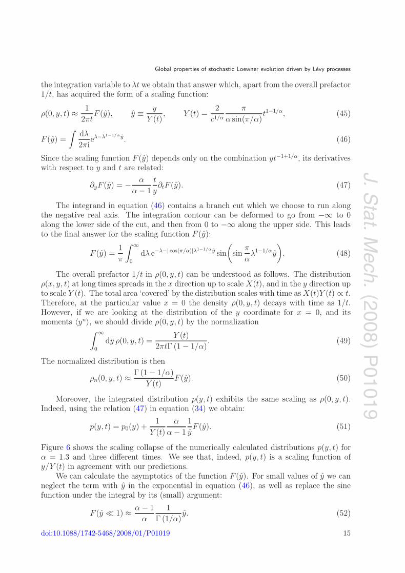
Figure 6 shows the scaling collapse of the numerically calculated distributions p(y, t) forα = 1.3 and three different times. We see that, indeed, p(y, t) is a scaling function ofy/Y (t) in agreement with our predictions.

We can calculate the asymptotics of the function F (y). For small values of y we canneglect the term with y in the exponential in equation (46), as well as replace the sinefunction under the integral by its (small) argument:

F (y � 1) ≈ α − 1

α

1

Γ (1/α)y. (52)

doi:10.1088/1742-5468/2008/01/P01019 15

J.Stat.M

ech.(2008)

P01019

Global properties of stochastic Loewner evolution driven by Levy processes

2 3 4

y/Y(t)

00 1

0.2

0.4

0.6

0.8

p( y

/Y(t

))t= 10000t= 30000t= 90000

α= 1.3

Figure 6. The distribution of heights scales as y/Y (t), where Y (t) is given byequation (45) for α = 1.3. The distribution is shown at three different times(black, red and green curves), all within the limiting region of large times whereasymptotic behavior y ∝ t1−1/α holds.

For large y we need to use the steepest descent method for the contour integral inequation (46), which results in

F (y 1) ≈(

α

2π

)1/2(α − 1

αy

)α/2

exp

[− 1

α − 1

(α − 1

αy

)α]. (53)

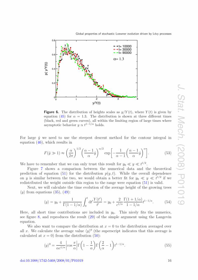
We have to remember that we can only trust this result for y0 � y � t1/2.Figure 7 shows a comparison between the numerical data and the theoretical

prediction of equation (51) for the distribution p(y, t). While the overall dependenceon y is similar between the two, we would obtain a better fit for y0 � y � t1/2 if weredistributed the weight outside this region to the range were equation (51) is valid.

Next, we will calculate the time evolution of the average height of the growing trees〈y〉 from equations (35), (49):

〈y〉 = y0 +1

Γ(1 − 1/α)

∫ t

0

dt′Y (t′)

t′= y0 +

2

c1/α

Γ(1 + 1/α)

1 − 1/αt1−1/α. (54)

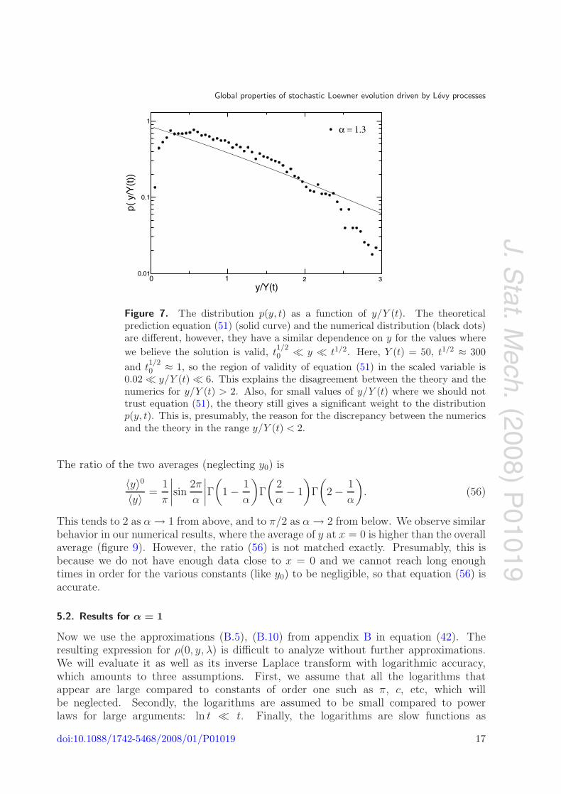
Here, all short time contributions are included in y0. This nicely fits the numerics,see figure 8, and reproduces the result (29) of the simple argument using the Langevinequation.

We also want to compare the distribution at x = 0 to the distribution averaged overall x. We calculate the average value 〈y〉0 (the superscript indicates that this average iscalculated at x = 0) from the distribution (50):

〈y〉0 =4

αc1/α

∣∣∣∣cosπ

α

∣∣∣∣Γ(

1 − 1

α

)Γ

(2

α− 1

)t1−1/α. (55)

doi:10.1088/1742-5468/2008/01/P01019 16

J.Stat.M

ech.(2008)

P01019

Global properties of stochastic Loewner evolution driven by Levy processes

0 1y/Y(t)

0.01

0.1

1

2 3

p( y

/Y(t

))α = 1.3

Figure 7. The distribution p(y, t) as a function of y/Y (t). The theoreticalprediction equation (51) (solid curve) and the numerical distribution (black dots)are different, however, they have a similar dependence on y for the values wherewe believe the solution is valid, t

1/20 � y � t1/2. Here, Y (t) = 50, t1/2 ≈ 300

and t1/20 ≈ 1, so the region of validity of equation (51) in the scaled variable is

0.02 � y/Y (t) � 6. This explains the disagreement between the theory and thenumerics for y/Y (t) > 2. Also, for small values of y/Y (t) where we should nottrust equation (51), the theory still gives a significant weight to the distributionp(y, t). This is, presumably, the reason for the discrepancy between the numericsand the theory in the range y/Y (t) < 2.

The ratio of the two averages (neglecting y0) is

〈y〉0〈y〉 =

1

π

∣∣∣∣sin 2π

α

∣∣∣∣Γ(

1 − 1

α

)Γ

(2

α− 1

)Γ

(2 − 1

α

). (56)

This tends to 2 as α → 1 from above, and to π/2 as α → 2 from below. We observe similarbehavior in our numerical results, where the average of y at x = 0 is higher than the overallaverage (figure 9). However, the ratio (56) is not matched exactly. Presumably, this isbecause we do not have enough data close to x = 0 and we cannot reach long enoughtimes in order for the various constants (like y0) to be negligible, so that equation (56) isaccurate.

5.2. Results for α = 1

Now we use the approximations (B.5), (B.10) from appendix B in equation (42). Theresulting expression for ρ(0, y, λ) is difficult to analyze without further approximations.We will evaluate it as well as its inverse Laplace transform with logarithmic accuracy,which amounts to three assumptions. First, we assume that all the logarithms thatappear are large compared to constants of order one such as π, c, etc, which willbe neglected. Secondly, the logarithms are assumed to be small compared to powerlaws for large arguments: ln t � t. Finally, the logarithms are slow functions as

doi:10.1088/1742-5468/2008/01/P01019 17

J.Stat.M

ech.(2008)

P01019

Global properties of stochastic Loewner evolution driven by Levy processes

0.0001 0.001 0.01 0.1 100 1000 10000 1e+051e+06

time

0.01

0.1

1

1

10

10

100

1000

10000

⟨y⟩

α= 1.3

Figure 8. The average height 〈y〉 for SLE driven by Levy flights with α = 1.3grows as a power law t1−1/α. The red dashed line is a fit to equation (54) fort > 1, where we only vary the parameter y0.

compared to power laws and exponentials, and in integrals can be replaced by theirvalues at the typical scale of variation of the fastest function under the integral. Allsubsequent equations in this section will be obtained with logarithmic accuracy using theseassumptions.

First we have

ρ(0, y, λ) ≈ 1

2π

ln 1λt0

ln cλy0

ln2 cλy

exp

(−c

2

y

ln cλy

). (57)

The time dependence now follows from the inverse Laplace transform, using the samecontour integral described in the previous section:

ρ(0, y, t) ≈ 1

2π2t

∫ ∞

0

dλln t

λt0ln ct

λy0

ln2 ctλy

sin

(π

2

cy

ln2 ctλy

)exp

(−λ − c

2

y

ln ctλy

). (58)

The integral of this expression over y∫ ∞

0

dy ρ(0, y, t) ≈ 1

πct

ln tt0

ln cty0

ln2(

c2t2

) (59)

leads to a normalized distribution at x = 0:

ρn(0, y, t) ≈ c

2π

ln2(c2t2

)

ln tt0

ln cty0

×∫ ∞

0

dλln t

λt0ln ct

λy0

ln2 ctλy

sin

(π

2

cy

ln2 ctλy

)exp

(−λ − c

2

y

ln ctλy

). (60)

doi:10.1088/1742-5468/2008/01/P01019 18

J.Stat.M

ech.(2008)

P01019

Global properties of stochastic Loewner evolution driven by Levy processes

0.001 0.01 0.1 1 10x/X(t)

0

50

100

150

200

⟨y⟩

α= 1.3

t= 3500t= 17000t= 90000

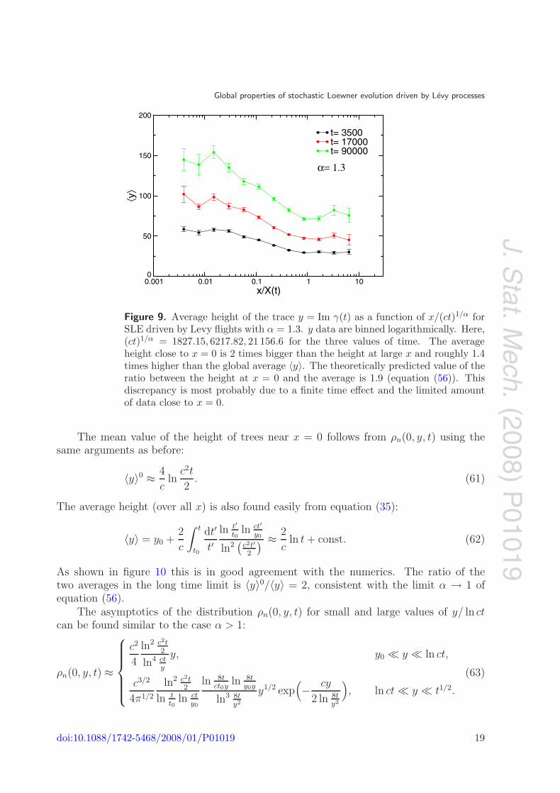
Figure 9. Average height of the trace y = Im γ(t) as a function of x/(ct)1/α forSLE driven by Levy flights with α = 1.3. y data are binned logarithmically. Here,(ct)1/α = 1827.15, 6217.82, 21 156.6 for the three values of time. The averageheight close to x = 0 is 2 times bigger than the height at large x and roughly 1.4times higher than the global average 〈y〉. The theoretically predicted value of theratio between the height at x = 0 and the average is 1.9 (equation (56)). Thisdiscrepancy is most probably due to a finite time effect and the limited amountof data close to x = 0.

The mean value of the height of trees near x = 0 follows from ρn(0, y, t) using thesame arguments as before:

〈y〉0 ≈ 4

cln

c2t

2. (61)

The average height (over all x) is also found easily from equation (35):

〈y〉 = y0 +2

c

∫ t

t0

dt′

t′

ln t′

t0ln ct′

y0

ln2(

c2t′

2

) ≈ 2

cln t + const. (62)

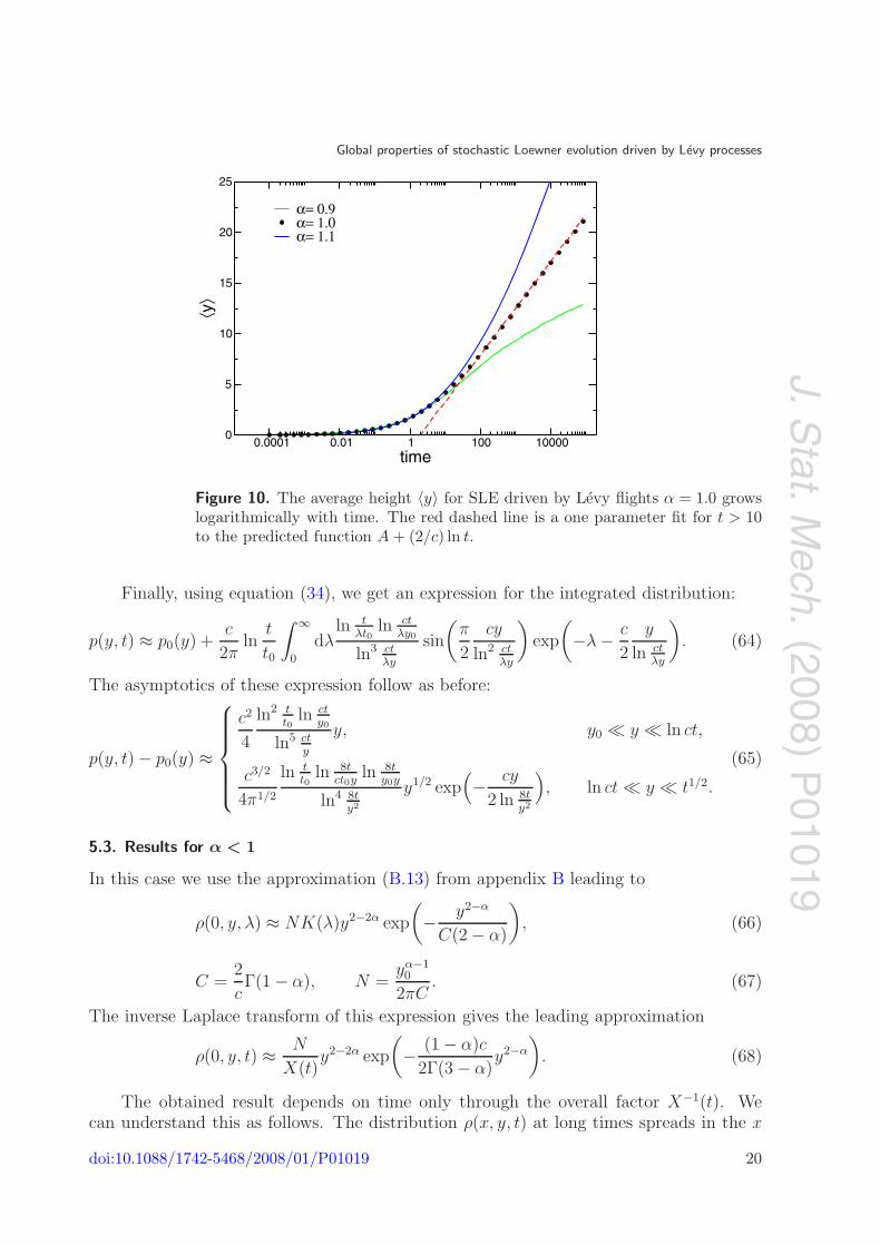
As shown in figure 10 this is in good agreement with the numerics. The ratio of thetwo averages in the long time limit is 〈y〉0/〈y〉 = 2, consistent with the limit α → 1 ofequation (56).

The asymptotics of the distribution ρn(0, y, t) for small and large values of y/ ln ctcan be found similar to the case α > 1:

ρn(0, y, t) ≈

⎧⎪⎪⎪⎪⎨⎪⎪⎪⎪⎩

c2

4

ln2 c2t2

ln4 cty

y, y0 � y � ln ct,

c3/2

4π1/2

ln2 c2t2

ln tt0

ln cty0

ln 8tct0y

ln 8ty0y

ln3 8ty2

y1/2 exp(− cy

2 ln 8ty2

), ln ct � y � t1/2.

(63)

doi:10.1088/1742-5468/2008/01/P01019 19

J.Stat.M

ech.(2008)

P01019

Global properties of stochastic Loewner evolution driven by Levy processes

0.0001 0.01 1 100 10000time

0

5

10

15

20

25

⟨y⟩

α= 0.9α= 1.0α= 1.1

Figure 10. The average height 〈y〉 for SLE driven by Levy flights α = 1.0 growslogarithmically with time. The red dashed line is a one parameter fit for t > 10to the predicted function A + (2/c) ln t.

Finally, using equation (34), we get an expression for the integrated distribution:

p(y, t) ≈ p0(y) +c

2πln

t

t0

∫ ∞

0

dλln t

λt0ln ct

λy0

ln3 ctλy

sin

(π

2

cy

ln2 ctλy

)exp

(−λ − c

2

y

ln ctλy

). (64)

The asymptotics of these expression follow as before:

p(y, t) − p0(y) ≈

⎧⎪⎪⎪⎪⎨⎪⎪⎪⎪⎩

c2

4

ln2 tt0

ln cty0

ln5 cty

y, y0 � y � ln ct,

c3/2

4π1/2

ln tt0

ln 8tct0y

ln 8ty0y

ln4 8ty2

y1/2 exp(− cy

2 ln 8ty2

), ln ct � y � t1/2.

(65)

5.3. Results for α < 1

In this case we use the approximation (B.13) from appendix B leading to

ρ(0, y, λ) ≈ NK(λ)y2−2α exp

(− y2−α

C(2 − α)

), (66)

C =2

cΓ(1 − α), N =

yα−10

2πC. (67)

The inverse Laplace transform of this expression gives the leading approximation

ρ(0, y, t) ≈ N

X(t)y2−2α exp

(− (1 − α)c

2Γ(3 − α)y2−α

). (68)

The obtained result depends on time only through the overall factor X−1(t). Wecan understand this as follows. The distribution ρ(x, y, t) at long times spreads in the x

doi:10.1088/1742-5468/2008/01/P01019 20

J.Stat.M

ech.(2008)

P01019

Global properties of stochastic Loewner evolution driven by Levy processes

100 5 15 20 25 30y

0.0001

0.001

0.01

0.1

1

p( y

, t)

α = 0.5 α = 0.7

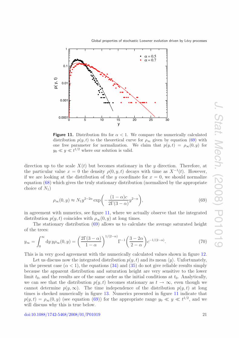
Figure 11. Distribution fits for α < 1. We compare the numerically calculateddistribution p(y, t) to the theoretical curve for ρ∞ given by equation (69) withone free parameter for normalization. We claim that p(y, t) = ρ∞(0, y) fory0 � y � t1/2 where our solution is valid.

direction up to the scale X(t) but becomes stationary in the y direction. Therefore, atthe particular value x = 0 the density ρ(0, y, t) decays with time as X−1(t). However,if we are looking at the distribution of the y coordinate for x = 0, we should normalizeequation (68) which gives the truly stationary distribution (normalized by the appropriatechoice of N1)

ρ∞(0, y) ≈ N1y2−2α exp

(− (1 − α)c

2Γ(3 − α)y2−α

), (69)

in agreement with numerics, see figure 11, where we actually observe that the integrateddistribution p(y, t) coincides with ρ∞(0, y) at long times.

The stationary distribution (69) allows us to calculate the average saturated heightof the trees:

y∞ =

∫ ∞

0

dy yρ∞(0, y) =

(2Γ(3 − α)

1 − α

)1/(2−α)

Γ−1

(3 − 2α

2 − α

)c−1/(2−α). (70)

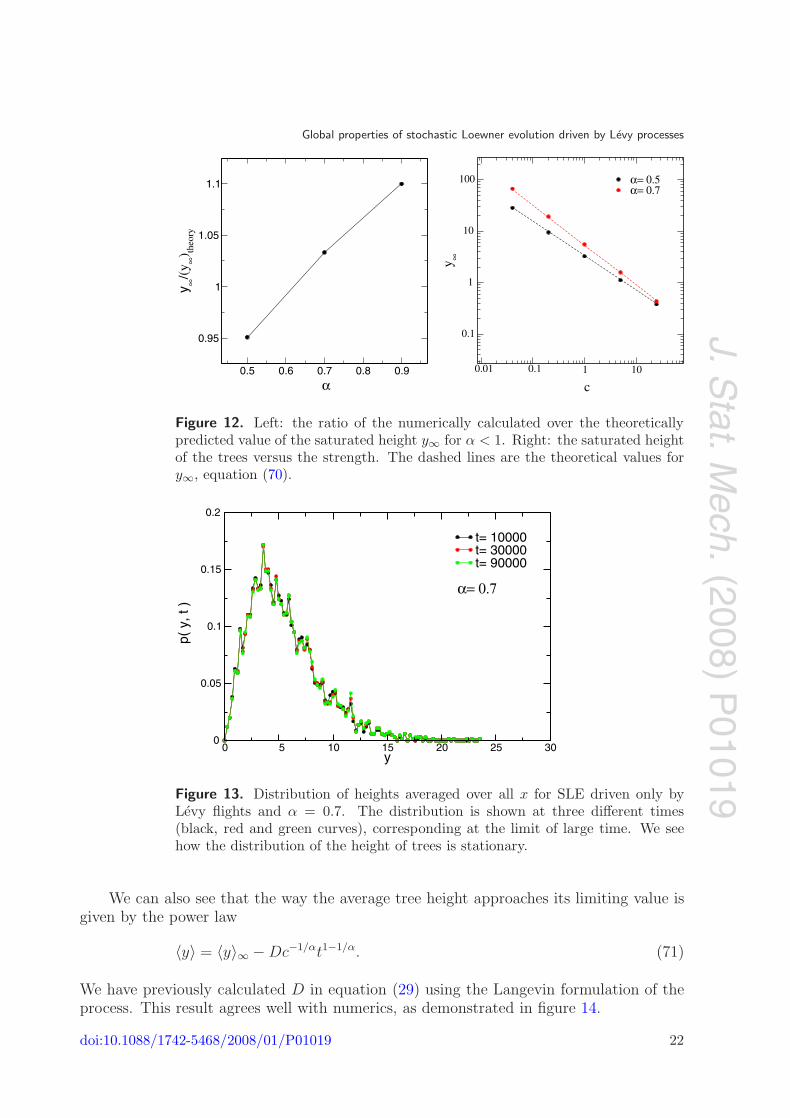
This is in very good agreement with the numerically calculated values shown in figure 12.Let us discuss now the integrated distribution p(y, t) and its mean 〈y〉. Unfortunately,

in the present case (α < 1), the equations (34) and (35) do not give reliable results simplybecause the apparent distribution and saturation height are very sensitive to the lowerlimit t0, and the results are of the same order as the initial conditions at t0. Analytically,we can see that the distribution p(y, t) becomes stationary as t → ∞, even though wecannot determine p(y,∞). The time independence of the distribution p(y, t) at longtimes is checked numerically in figure 13. Numerics presented in figure 11 indicate thatp(y, t) = ρ∞(0, y) (see equation (69)) for the appropriate range y0 � y � t1/2, and wewill discuss why this is true below.

doi:10.1088/1742-5468/2008/01/P01019 21

J.Stat.M

ech.(2008)

P01019

Global properties of stochastic Loewner evolution driven by Levy processes

0.5 0.6 0.7 0.8 0.9 α

0.95

1

1.05

1.1y ∞

/(y ∞

) theo

ry

0.01 0.1

c

0.1

1

1

10

10

100

y ∞

α= 0.5α= 0.7

Figure 12. Left: the ratio of the numerically calculated over the theoreticallypredicted value of the saturated height y∞ for α < 1. Right: the saturated heightof the trees versus the strength. The dashed lines are the theoretical values fory∞, equation (70).

0 5 10 15 20 25 30y

0

0.05

0.1

0.15

0.2

p( y

, t )

t= 10000t= 30000t= 90000

α= 0.7

Figure 13. Distribution of heights averaged over all x for SLE driven only byLevy flights and α = 0.7. The distribution is shown at three different times(black, red and green curves), corresponding at the limit of large time. We seehow the distribution of the height of trees is stationary.

We can also see that the way the average tree height approaches its limiting value isgiven by the power law

〈y〉 = 〈y〉∞ − Dc−1/αt1−1/α. (71)

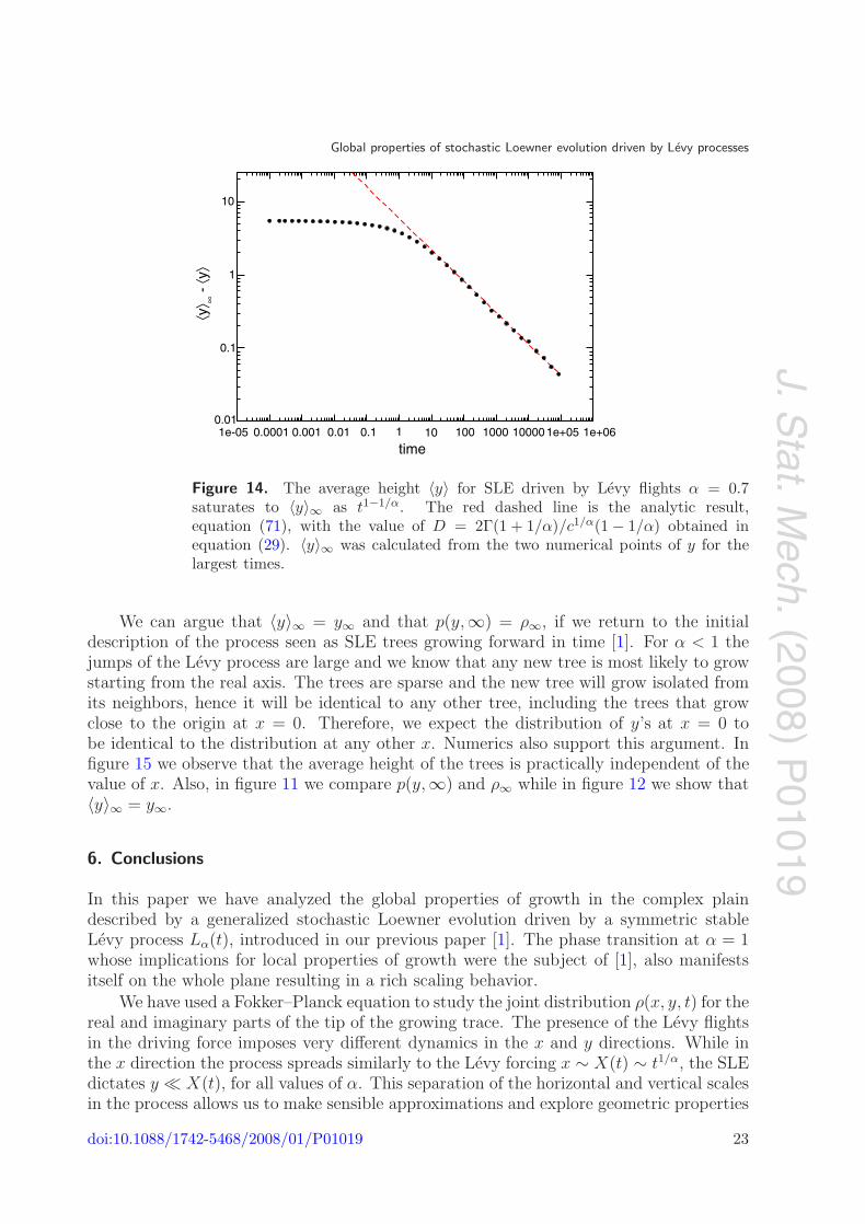
We have previously calculated D in equation (29) using the Langevin formulation of theprocess. This result agrees well with numerics, as demonstrated in figure 14.

doi:10.1088/1742-5468/2008/01/P01019 22

J.Stat.M

ech.(2008)

P01019

Global properties of stochastic Loewner evolution driven by Levy processes

1e-05 0.0001 0.001 0.01 0.1 100 1000 10000 1e+05 1e+06

time

0.01

0.1

1

1

10

10

⟨y⟩ ∞

- ⟨y

⟩

Figure 14. The average height 〈y〉 for SLE driven by Levy flights α = 0.7saturates to 〈y〉∞ as t1−1/α. The red dashed line is the analytic result,equation (71), with the value of D = 2Γ(1 + 1/α)/c1/α(1 − 1/α) obtained inequation (29). 〈y〉∞ was calculated from the two numerical points of y for thelargest times.

We can argue that 〈y〉∞ = y∞ and that p(y,∞) = ρ∞, if we return to the initialdescription of the process seen as SLE trees growing forward in time [1]. For α < 1 thejumps of the Levy process are large and we know that any new tree is most likely to growstarting from the real axis. The trees are sparse and the new tree will grow isolated fromits neighbors, hence it will be identical to any other tree, including the trees that growclose to the origin at x = 0. Therefore, we expect the distribution of y’s at x = 0 tobe identical to the distribution at any other x. Numerics also support this argument. Infigure 15 we observe that the average height of the trees is practically independent of thevalue of x. Also, in figure 11 we compare p(y,∞) and ρ∞ while in figure 12 we show that〈y〉∞ = y∞.

6. Conclusions

In this paper we have analyzed the global properties of growth in the complex plaindescribed by a generalized stochastic Loewner evolution driven by a symmetric stableLevy process Lα(t), introduced in our previous paper [1]. The phase transition at α = 1whose implications for local properties of growth were the subject of [1], also manifestsitself on the whole plane resulting in a rich scaling behavior.

We have used a Fokker–Planck equation to study the joint distribution ρ(x, y, t) for thereal and imaginary parts of the tip of the growing trace. The presence of the Levy flightsin the driving force imposes very different dynamics in the x and y directions. While inthe x direction the process spreads similarly to the Levy forcing x ∼ X(t) ∼ t1/α, the SLEdictates y � X(t), for all values of α. This separation of the horizontal and vertical scalesin the process allows us to make sensible approximations and explore geometric properties

doi:10.1088/1742-5468/2008/01/P01019 23

J.Stat.M

ech.(2008)

P01019

Global properties of stochastic Loewner evolution driven by Levy processes

0.001 0.01 0.1 1 10 100x/XL(t)

0

1

2

3

4

5

6

7

8

9

10

⟨y⟩

t= 3500t= 17000t= 90000

α= 0.7

Figure 15. Average height of the trace y = Im γ(t) as a function of x/(ct)1/α forSLE driven by Levy flights with α = 0.7. y data are binned logarithmically andthe average of every bin is plotted. (ct)1/α = 2.9 × 105, 2.8 × 106, 2.75 × 107.

of the stochastic growth in all phases, α < 1, α = 1, and α > 1, both qualitatively andquantitatively.

For α < 1, the vertical growth saturates at a finite height y∞. In terms of the picturepresented in [1], long jumps occur often so that new trees grow isolated and there is asmall chance that the trace grows on an already existing tree.

For α > 1, the average height of the process grows as a power law t1−1/α with time.New trees grow close to old ones, so that when the process returns to a previously visitedpart of the real axis it will have to grow on top of already existing trees. Eventually thetrace will grow past any point on the plane.

At the boundary between the two phases, α = 1, the height of the process growslogarithmically with time.

Acknowledgments

This research was supported in part by NSF MRSEC Program under DMR-0213745.IG was also supported by an award from Research Corporation and the NSF CareerAward under DMR-0448820. We wish to acknowledge many helpful discussions withPaul Wiegmann, Eldad Bettelheim, and Seung Yeop Lee. IG also acknowledges usefulcommunications with Steffen Rohde.

Appendix A. Numerical calculations

The interpretation of equation (16) is very helpful to our calculations. zt and the tip ofthe trace have the same distribution. This allows, instead of calculating the trace γ(t) forevery time t and noise realization (O(n2)), to efficiently collect statistics for the positionof the tip by integrating the Langevin equation (16) (O(n)).

doi:10.1088/1742-5468/2008/01/P01019 24

J.Stat.M

ech.(2008)

P01019

Global properties of stochastic Loewner evolution driven by Levy processes

Following [1] we approximate ξ(t) by a piecewise constant function with jumpsappropriately distributed: ξ(t) = ξj for (j − 1)τ < t < jτ . For such a driving functionthe process zt in equation (16) can then be calculated numerically as an iteration processof infinitesimal maps [24] starting from the condition z = 0 as follows:

zn = z(nτ) = fn ◦ fn−1 . . . ◦ f1(0) − ξn. (A.1)

The infinitesimal conformal map fn at each time interval n is defined by:

fn(z) = w−1n (z) =

√(z − ξn)2 − 4τ + ξn. (A.2)

The value of ξn is randomly drawn from the appropriate distribution. The number ofsteps necessary to produce an SLE trace up to step n grows only as O(n). All numericalresults in the next section have been calculated using the average of equation (A.2) overmany noise realizations.

The trace can also be produced directly [1], as g−1(ξ(t), t), in which case weapproximate

γj = γ(jτ) = f1 . . . ◦ fn−1 ◦ fn(ξn). (A.3)

However, the number of steps in this method grows as O(n2). We used this method toverify that numerically calculated z and γ have identical distributions. Equation (A.3)was also used to calculate the traces shown in figure 2.

Here, we will assume κ = 0 for simplicity, that is, the driving force is pure Levy flightsξ(t) = c1/αLα(t). The addition of a Brownian motion will not affect our conclusions. Forall realizations of the Levy-SLE process we take c = 1 and τ = 10−4 unless otherwisenoted.

Appendix B. Asymptotics for K(λ, y)

Let us consider (we need to use the lower cut off t0 here to have a convergent result forα < 1)

K(λ) =

∫ ∞

t0

dte−λt

X(t)=

2Γ (1 + 1/α)

c1/α

∫ ∞

t0

dt t−1/αe−λt

=

⎧⎪⎨⎪⎩

2Γ(1 + 1/α)

c1/αλ−1+1/αΓ

(1 − 1

α, λt0

), α �= 1,

2

cE1(λt0), α = 1,

(B.1)

where Γ(a, x) is the incomplete gamma function, and E1(x) is the exponential integral.Since λ has the dimension and the meaning of frequency, and we are interested in t t0,we will only need the small argument asymptotics of these functions:

Γ(a, x) ≈ Γ(a) − xa

a, E1(x) ≈ − ln x, x � 1. (B.2)

doi:10.1088/1742-5468/2008/01/P01019 25

J.Stat.M

ech.(2008)

P01019

Global properties of stochastic Loewner evolution driven by Levy processes

This gives for λt0 � 1

K(λ) ≈ Aλ−1+1/α + Bt1−1/α0 , α �= 1, (B.3)

A =2π

αc1/α sin(π/α), B =

2

c1/α

α

1 − αΓ

(1 +

1

α

), (B.4)

K(λ) ≈ 2

cln

1

λt0, α = 1. (B.5)

For α > 1 we can set t0 = 0 and obtain

K(λ) = Aλ−1+1/α, α > 1, (B.6)

and for α < 1 we can set λ = 0:

K(0) = Bt1−1/α0 , α < 1. (B.7)

We now turn to the Laplace transform K(λ, y):

K(λ, y) = 2

∫ ∞

0

dke−yk

λ + ckα. (B.8)

Since in the Laplace transform the important values of λ are the inverse typical timescales,this means that the relevant asymptotics of K(λ, y) are those with λyα/c � 1. Theopposite case of λyα/c 1 corresponds to short times, where our basic approximation isinvalid. So from now on we will focus on the limit λyα/c � 1.

This integral can be evaluated exactly in a number of cases. First, when y = 0, theintegral converges for α > 1 and gives the same expression as K(λ) in equation (B.6).Secondly, for λ = 0 the integral converges (for y > 0) for α < 1 and gives then

K(0, y) =2

c

∫ ∞

0

dk k−αe−yk = Cyα−1, C =2

cΓ(1 − α). (B.9)

All the constants A, B, and C defined above diverge as 1/(α − 1) as α → 1. Finally, forα = 1 we get

K(λ, y) =2

ceλy/cE1

(λy

c

)≈ 2

cln

c

λy,

λy

c� 1. (B.10)

In general for λyα/c � 1, a good approximation for K(λ, y) is the sum of expressionsin equations (B.6) and (B.9):

K(λ, y) ≈ Aλ−1+1/α + Cyα−1. (B.11)

Not only this approximation reproduces the correct limits in equations (B.6) and (B.9),but in the limit α → 1 it also reduces to equation (B.10). This approximation can beobtained by splitting the k interval in the integral in equation (B.8) into two at the valuek0 = (λ/c)1/α and in each resulting integral replace the denominator by the largest termin it.

Notice that for α > 1, and in the limit of interest λyα/c � 1 the first term inequation (B.11) is much greater than the second, and we can use equation (B.6) for bothK(λ) and K(λ, y):

K(λ) ≈ K(λ, y) ≈ Aλ−1+1/α, α > 1. (B.12)

For α < 1 the opposite is true, and we can use equation (B.9) as a valid approximation:

K(λ, y) ≈ Cyα−1, C =2

cΓ(1 − α). (B.13)

doi:10.1088/1742-5468/2008/01/P01019 26

J.Stat.M

ech.(2008)

P01019

Global properties of stochastic Loewner evolution driven by Levy processes

References

[1] Rushkin I, Oikonomou P, Kadanoff L P and Gruzberg I A, 2006 J. Stat. Mech. P01001[cond-mat/0509187]

[2] Schramm O, 2000 Isr. J. Math. 118 221 [math.PR/9904022][3] Lawler G F, Conformally invariant processes in the plane, 2005 Mathematical Surveys and Monographs

vol 114 (Providence, RI: American Mathematical Society)[4] Werner W, Random planar curves and Schramm–Loewner evolutions, 2004 Springer Lecture Notes in

Mathematics vol 1840 (Berlin: Springer) [math.PR/0303354][5] Schramm O, Conformally invariant scaling limits: an overview and a collection of problems, 2007 Proc.

International Congress of Mathematicians (Madrid, 2006) vol I (Zurich: European Mathematical Society)pp 513–43 [math.PR/0602151]

[6] Bauer M and Bernard D, 2006 Phys. Rep. 432 115 [math-ph/0602049][7] Cardy J, 2005 Ann. Phys., NY 318 81 [cond-mat/0503313][8] Gruzberg I A, 2006 J. Phys. A: Math. Gen. 39 12601 [math-ph/0607046][9] Gruzberg I A and Kadanoff L P, 2004 J. Stat. Phys. 114 1183 [cond-mat/0309292]

[10] Kager W and Nienhuis B, 2004 J. Stat. Phys. 115 1149 [math-ph/0312056][11] Guan Q and Winkel M, 2006 Preprint math.PR/0606685[12] Guan Q, 2007 Preprint 0705.2321 [math.PR][13] Chen Z-Q and Rohde S, 2007 Preprint 0708.1805 v2 [math.PR][14] Beliaev D and Smirnov S, Harmonic measure and SLE , 2008 Preprint 0801.1792v1 [math.CV][15] Duplantier B, 2000 Phys. Rev. Lett. 84 1363 [cond-mat/9908314][16] Duplantier B, 2004 Fractal Geometry and Applications: a Jubilee of Benoıt Mandelbrot. Part 2:

Multifractals, Probability and Statistical Mechanics, Applications. Proc. Special Session of the AnnualMeeting of the American Mathematical Society (San Diego, CA, January 2002) (Proc. Symp. PureMath. 72) ed M L Lapidus and M van Frankenhuijsen (Providence, RI: American Mathematical Society)p 365 [math-ph/0303034]

[17] Bettelheim E, Rushkin I, Gruzberg I A and Wiegmann P, 2005 Phys. Rev. Lett.95 170602 [hep-th/0507115]

[18] Rushkin I, Bettelheim E, Gruzberg I A and Wiegmann P, 2007 J. Phys. A: Math. Theor.40 2165 [cond-mat/0610550]

[19] Rohde S and Schramm O, 2005 Ann. Math. 161(2) 883 [math.PR/0106036][20] Appelbaum D, 2004 Levy Processes and Stochastic Calculus (Cambridge: Cambridge University Press)[21] Metzler R and Klafter J, 2000 Phys. Rep. 339 1[22] Samorodnitsky G and Taqqu M S, 1994 Stable Non-Gaussian Random Processes: Stochastic Models with

Infinite Variance (London: Chapman and Hall)[23] Sato K, 1999 Levy Processes and Infinitely Divisible Distributions (Cambridge: Cambridge University

Press)[24] Hastings M B, 2002 Phys. Rev. Lett. 88 055506 [cond-mat/9607021]

doi:10.1088/1742-5468/2008/01/P01019 27