Journal of Functional Analysis 203 (2003) 262–285

On a type of stochastic differential equationsdriven by countably many Brownian motions

Guilan Cao and Kai He�

Department of Mathematics, Huazhong University of Science and Technology, Wuhan, Hubei 430074,

People’s Republic of China

Received 10 July 2002; accepted 12 December 2002

Abstract

Consider the one-dimensional SDE Xt ¼ x þP

N

i¼1R t

0siðXsÞ dW i

s þR t

0bðXsÞ ds; where W i is

an infinite sequence of independent standard Brownian motions, i ¼ 1; 2; 3;y :We prove two

theorems on the existence and uniqueness of solutions with non-Lipschitz coefficients, and

give a non-contact property and a strong comparison theorem for solutions.

r 2003 Elsevier Science (USA). All rights reserved.

Keywords: One-dimensional SDE; Existence; Uniqueness; Non-contact property; Strong comparison

theorem

1. Introduction

The following classical SDE

dXt ¼ sðXtÞ dWt þ bðXtÞ dt

X0 ¼ x

(ð1:1Þ

is well known, where sðxÞ is a Borel measurable function Rm-Rm#Rd ; bðxÞ is aBorel measurable function Rm-Rm; and W is a d-dimensional standard Brownianmotion. In the case where s and b satisfy a Lipschitz condition or satisfy a locallyLipschitz condition plus a linear growth condition, Eq. (1.1) has a unique strongsolution. Later, Yamada and Watanabe [14] developed the theory on the uniqueness

ARTICLE IN PRESS

�Corresponding author.

E-mail addresses: cglhust@sohu.com (G. Cao), hekai0@sina.com (K. He).

0022-1236/03/$ - see front matter r 2003 Elsevier Science (USA). All rights reserved.

doi:10.1016/S0022-1236(03)00066-1

of solutions when m ¼ d ¼ 1: They got the best Holder conditions on the coefficientsof one-dimensional SDE. In this case, Yamada and Ogura [13] gave some non-contact properties and strong comparison theorems. Perkins [10] realized that theuse of semimartingale local time provided a unified framework and simplified theproof for one-dimensional SDE. And using local time in a quite different way,Le Gall [4] provided a short and simple proof of the classic Yamada and Watanabe’sresult.In this paper, motivated by Yamada’s work and the recent work of Airault, Ren

and Malliavin, we consider the following one-dimensional SDE:

dXt ¼PNi¼1

siðXtÞ dW it þ bðXtÞ dt ðt40Þ;

X0 ¼ x;

8><>: ð1:2Þ

where siðxÞ and bðxÞ are Borel measurable functions R-R; and W i is an infinitesequence of independent standard Brownian motions, i ¼ 1; 2; 3;y : The maindifference between this type of equations and the classical ones with finite manyBrownian motions is that it seems difficult to obtain the unique strong solution bythe usual weak solution plus pathwise uniqueness procedure. The purpose of thepresent paper is to study the existence and uniqueness of solutions to Eq. (1.2) withnon-Lipschitz coefficients by using a Picard-type iteration and semimartingale localtime. Finally, we shall give a non-contact property and a strong comparison theoremfor solutions.This paper is organized as follows. In Section 2, we first give necessary notations

and notions. In Section 3, we state and prove our main result. And then in Section 4,we present the non-contact property and strong comparison theorem. In the end, inSection 5, we give a example which includes the SDE considered in [1] as a specialcase.

2. Notations and notions

Let siðxÞ and bðxÞ be Borel measurable functions R-R; i ¼ 1; 2; 3;y : Considerthe following one-dimensional SDE:

dXt ¼PNi¼1

siðXtÞ dW it þ bðXtÞ dt ðt40Þ;

X0 ¼ xAR;

8><>:

namely,

Xt ¼ x þXNi¼1

Z t

0

siðXsÞ dW is þ

Z t

0

bðXsÞ ds; ð2:1Þ

ARTICLE IN PRESSG. Cao, K. He / Journal of Functional Analysis 203 (2003) 262–285 263

where W i is an infinite sequence of independent standard Brownian motions,i ¼ 1; 2; 3;y : Set

sðxÞ ¼ ðs1ðxÞ; s2ðxÞ;yÞ;

jsðxÞj ¼PNi¼1

s2i ðxÞ �1

2:

8>><>>:

Suppose sðxÞAl2 for all xAR: We denote a4b ¼ minða; bÞ; and a3b ¼ maxða; bÞ:Firstly, we will define stochastic integrals with respect to countably many

Brownian motions.

Lemma 2.1. Let ðFtÞtX0 be a right-continuous complete s-algebras filtration

generated by W i; i ¼ 1; 2; 3;y : Given two sequences of measurable ðFtÞ-adapted

processes Hi and Gi; set

Mt ¼PNi¼1

R t

0 HiðsÞ dW is ;

Nt ¼PNi¼1

R t

0 GiðsÞ dW is :

8>><>>:

If jHj ¼ ðP

N

i¼1 H2i Þ

12AH2

loc; i.e.

Z t

0

EjHðsÞj2 dsoN

for all tX0; then M is a continuous L2ðFtÞ-martingale. If jHjAL2loc; i.e.

Z t

0

jHðsÞj2 dsoN a:s:

for all tX0; then M is a continuous local ðFtÞ-martingale. The quadratic variation of

M is

½M�t ¼Z t

0

jHðsÞj2 ds

for all tX0; and the cross variation of M and N is

½M;N�t ¼XNi¼1

Z t

0

HiðsÞGiðsÞ ds

for all tX0:

ARTICLE IN PRESSG. Cao, K. He / Journal of Functional Analysis 203 (2003) 262–285264

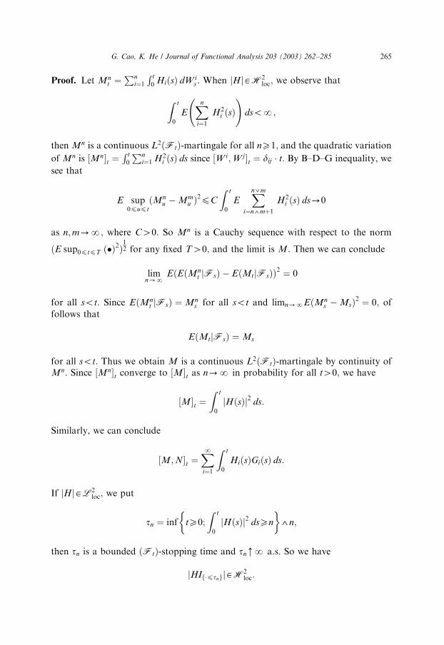
Proof. Let Mnt ¼

Pni¼1R t

0 HiðsÞ dW is : When jHjAH2

loc; we observe that

Z t

0

EXn

i¼1H2

i ðsÞ !

dsoN;

then Mn is a continuous L2ðFtÞ-martingale for all nX1; and the quadratic variation

of Mn is ½Mn�t ¼R t

0

Pni¼1 H2

i ðsÞ ds since ½W i;W j�t ¼ dij t: By B–D–G inequality, we

see that

E sup0pupt

ðMnu Mm

u Þ2pC

Z t

0

EXn3m

i¼n4mþ1H2

i ðsÞ ds-0

as n;m-N; where C40: So Mn is a Cauchy sequence with respect to the norm

ðE sup0ptpT ð�Þ2Þ12 for any fixed T40; and the limit is M: Then we can conclude

limn-N

EðEðMnt jFsÞ EðMtjFsÞÞ2 ¼ 0

for all sot: Since EðMnt jFsÞ ¼ Mn

s for all sot and limn-NEðMns MsÞ2 ¼ 0; of

follows that

EðMtjFsÞ ¼ Ms

for all sot: Thus we obtain M is a continuous L2ðFtÞ-martingale by continuity ofMn: Since ½Mn�t converge to ½M�t as n-N in probability for all t40; we have

½M�t ¼Z t

0

jHðsÞj2 ds:

Similarly, we can conclude

½M;N�t ¼XNi¼1

Z t

0

HiðsÞGiðsÞ ds:

If jHjAL2loc; we put

tn ¼ inf tX0;

Z t

0

jHðsÞj2 dsXn

� �4n;

then tn is a bounded ðFtÞ-stopping time and tnmN a.s. So we have

jHIfptngjAH2loc:

ARTICLE IN PRESSG. Cao, K. He / Journal of Functional Analysis 203 (2003) 262–285 265

Therefore,

Y nt ¼

XNi¼1

Z t

0

HiðsÞIfsptng dW is

is a continuous L2ðFtÞ-martingale for all nX1: It is easy to see that ðY mÞtn ¼ Y n forall mXn: Thus, there exist a unique continuous local ðFtÞ-martingale M such thatMtn ¼ Y n: &

Secondly, we will state several properties of stochastic integrals with respect tocountably many Brownian motions.

(1) If jHj and jGjAL2loc; then jaH þ bGjAL2

loc for all a; bAR; and it holds

XNi¼1

Z t

0

ðaHiðsÞ þ bGiðsÞÞ dW is ¼ a

XNi¼1

Z t

0

HiðsÞ dW is þ b

XNi¼1

Z t

0

GiðsÞ dW is

for all tX0:(2) Under the conditions of Lemma 2.1, if f is a measurable ðFtÞ-adapted process

such that jfHjAL2loc; then

R t

0fs d½M�s ¼

PNi¼1

R t

0fsH

2s ðsÞ ds;

R t

0 fs dMs ¼PNi¼1

R t

0 fsHiðsÞ dW is

8>><>>:

for all tX0:(3) By (2) and Lemma 2.1, we can use Ito’s formula, Tanaka’s formula and B–D–

G inequality on stochastic integrals with respect to countably many Brownianmotions.The proof of properties (1)–(3) is done by usual methods, therefore,

we omit it.

3. Existence and uniqueness theorem

Theorem 3.1. Let r; g be concave non-decreasing continuous functions on Rþ such that

rð0Þ ¼ 0; gð0Þ ¼ 0: For all x; yAR;

jsðxÞ sðyÞjprðjx yjÞ;jbðxÞ bðyÞjpgðjx yjÞ:

(

ARTICLE IN PRESSG. Cao, K. He / Journal of Functional Analysis 203 (2003) 262–285266

If there exist a constant pX2 such thatZ0þ

xp1 dx

rpðxÞ þ gpðxÞ ¼ N;

then Eq. (2.1) has a unique solution.

Remark. (1) If there exist a complete probability space ðO;F;PÞ; a right-continuouscomplete s-algebras filtration ðFtÞtX0 which is sub s-algebras of F; an infinite

sequence of independent standard Brownian motions W i; a continuous ðFtÞ-adapted process X such that bðXÞAL1

loc and jsðX ÞjAL2loc; which satisfy Eq. (2.1),

we will call X plus W i is a solution of Eq. (2.1) with initial value x: ‘‘Uniqueness’’

here means that if X 1;X 2 are two solutions of Eq. (2.1) defined on the same

probability space, then PðX 1t ¼ X 2

t ; for all tARþÞ ¼ 1:(2) Under the conditions of Theorem 3.1 we can concludeR

0þ rpðxÞ dx ¼ N;R

0þ gpðxÞ dx ¼ N:

(

(3) Let us take

r1ðxÞ ¼ Kx;

i.e. s satisfies Lipschitz condition, or let

r2ðxÞ ¼0; x ¼ 0;

Kxðlog 1xÞa; 0oxpd;

Kdðlog 1dÞ

a; x4d;

8><>:

where ap12; or take

r3ðxÞ ¼0; x ¼ 0;

Kxðlog 1xÞ1=3 log log 1

x; 0oxpd;

Kdðlog 1dÞ1=3 log log 1

d; x4d;

8>><>>:

where K40 and dAð0; 1Þ is sufficiently small. They all satisfy the conditions ofTheorem 3.1 at the case of p ¼ 2:

Lemma 3.2. Under the conditions of Theorem 3.1, s; b are continuous functions on R;and there exist some constants Kr40 such that

jsðxÞjrpKrð1þ rrðjxjÞÞ;jbðxÞjrpKrð1þ grðjxjÞÞ

(ð3:1Þ

for all rX0: So sðxÞAl2 for all xAR:

ARTICLE IN PRESSG. Cao, K. He / Journal of Functional Analysis 203 (2003) 262–285 267

Proof. Take y ¼ 0 and then use the Cr inequality. &

Firstly, we need to prepare a series of lemmas, which are necessary for provingTheorem 3.1.The following result is obvious.

Lemma 3.3. If r is a concave continuous function on Rþ such that rð0Þ ¼ 0; then there

exist some constants Kr40 such that rrðjxjÞpKrð1þ jxjrÞ for all rX0:

Corollary 3.4. Under the conditions of Theorem 3.1, there exist some constants Kr40such that

jsðxÞjr þ jbðxÞjrpKrð1þ jxjrÞ

for all rX0; i.e. s and b satisfy the linear growth condition.

Proof. It comes from Corollary 3.2 and Lemma 3.3. &

Lemma 3.5. Let r be a concave non-decreasing continuous functions on Rþ such that

rð0Þ ¼ 0: Then gðxÞ ¼ rrðx1sÞ is also a concave non-decreasing continuous function on

Rþ such that gð0Þ ¼ 0 for all sXrX1:

Proof. Clearly, g is a non-decreasing continuous function on Rþ such that gð0Þ ¼ 0:

We can also have rðxÞx

is a non-negative non-increasing continuous function on

ð0;NÞ and r0þ is a non-negative non-increasing right-continuous function on ð0;NÞ:So we obtain

g0þðxÞ ¼

r

srr1ðx

1sÞx

1ss r0þðx

1sÞ ¼ r

s

rðx1=sÞx1=s

�r11

x1r=sr0þðx

1sÞ

is a non-negative non-increasing right-continuous function on ð0;NÞ: Thus we canconclude g is a concave function. &

Corollary 3.6. Under the conditions of Theorem 3.1, let f ðxÞ ¼ rpðx1pÞ þ gpðx

1pÞ for all

xX0; then f is a concave non-decreasing continuous function on Rþ such that f ð0Þ ¼ 0

andR0þ f 1ðxÞ dx ¼ N:

Proof. Use Lemma 3.5 andR d0þ f 1ðxÞ dx ¼ p

R d1p0þ

xp1 dxrpðxÞþgpðxÞ: &

We have the following result by Comparison Theorem.

ARTICLE IN PRESSG. Cao, K. He / Journal of Functional Analysis 203 (2003) 262–285268

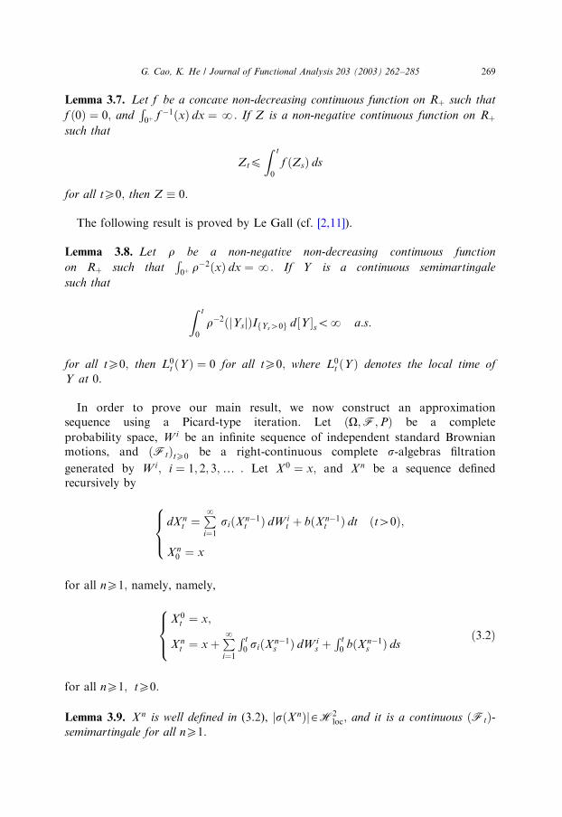
Lemma 3.7. Let f be a concave non-decreasing continuous function on Rþ such that

f ð0Þ ¼ 0; andR0þ f 1ðxÞ dx ¼ N: If Z is a non-negative continuous function on Rþ

such that

ZtpZ t

0

f ðZsÞ ds

for all tX0; then Z � 0:

The following result is proved by Le Gall (cf. [2,11]).

Lemma 3.8. Let r be a non-negative non-decreasing continuous function

on Rþ such thatR0þ r

2ðxÞ dx ¼ N: If Y is a continuous semimartingale

such that

Z t

0

r2ðjYsjÞIfYs40g d½Y �soN a:s:

for all tX0; then L0t ðYÞ ¼ 0 for all tX0; where L0

t ðYÞ denotes the local time of

Y at 0.

In order to prove our main result, we now construct an approximationsequence using a Picard-type iteration. Let ðO;F;PÞ be a complete

probability space, W i be an infinite sequence of independent standard Brownianmotions, and ðFtÞtX0 be a right-continuous complete s-algebras filtration

generated by W i; i ¼ 1; 2; 3;y : Let X 0 ¼ x; and X n be a sequence definedrecursively by

dX nt ¼

PNi¼1

siðX n1t Þ dW i

t þ bðX n1t Þ dt ðt40Þ;

X n0 ¼ x

8><>:

for all nX1; namely, namely,

X 0t ¼ x;

X nt ¼ x þ

PNi¼1

R t

0 siðX n1s Þ dW i

s þR t

0 bðX n1s Þ ds

8><>: ð3:2Þ

for all nX1; tX0:

Lemma 3.9. X n is well defined in (3.2), jsðX nÞjAH2loc; and it is a continuous ðFtÞ-

semimartingale for all nX1:

ARTICLE IN PRESSG. Cao, K. He / Journal of Functional Analysis 203 (2003) 262–285 269

Proof. For all nX1; 0ptpT ; from (3.2) and Corollary 3.4, we have

EðX nt Þ

2p 3x2 þ 3EXNi¼1

Z t

0

siðX n1s Þ dW i

s

!2

þ3E

Z t

0

bðX n1s Þ ds

�2

p 3x2 þ 3

Z t

0

EjsðX n1s Þj2 ds þ 3T

Z t

0

Eðb2ðX n1s ÞÞ ds

p 3x2 þ 3K2ðT þ 1ÞZ t

0

ð1þ EðX n1s Þ2Þ ds

¼ 3x2 þ 3K2TðT þ 1Þ 1þ sup0ptpT

EðX n1t Þ2

�;

then we deduce

sup0ptpT

EðX nt Þ

2p3x2 þ 3K2TðT þ 1Þ 1þ sup0ptpT

EðX n1t Þ2

�:

By sup0ptpT EðX 0t Þ

2 ¼ x2oN; then

sup0ptpT

EðX nt Þ

2oN;

for all nX1: Using Corollary 3.4, we see that

Z t

0

EjsðX ns Þj

2dspK2T 1þ sup

0ptpT

EðX nt Þ

2

�oN;

i.e.

jsðX nÞjAH2loc:

Thus we obtain X n is well defined, and it is a continuous ðFtÞ-semimartingale for allnX1 by Lemma 2.1. &

Lemma 3.10. Under the conditions of Theorem 3.1, for any fixed T40; there exist

some constants Cr;T40 such that

E sup0pupt

jX nu j

rpCr;T ;

E sup0pupt

jX nu X m

u jrpCr;T

8>><>>:

for all n;mX1; rX2; 0ptpT :

ARTICLE IN PRESSG. Cao, K. He / Journal of Functional Analysis 203 (2003) 262–285270

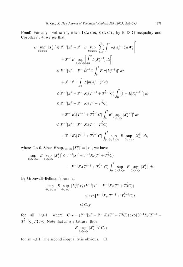
Proof. For any fixed mX1; when 1pnpm; 0ptpT ; by B–D–G inequality andCorollary 3.4, we see that

E sup0pupt

jX nu j

rp 3r1jxjr þ 3r1E sup0pupt

XNi¼1

Z u

0

siðX n1s Þ dW i

s

����������r

þ 3r1E sup0pupt

Z u

0

bðX n1s Þ ds

��������r

p 3r1jxjr þ 3r1tr21C

Z t

0

EjsðX n1s Þjr ds

þ 3r1tr1Z t

0

EjbðX n1s Þjr ds

p 3r1jxjr þ 3r1KrðTr1 þ Tr21CÞ

Z t

0

ð1þ EjX n1s jrÞ ds

p 3r1jxjr þ 3r1KrðTr þ Tr2CÞ

þ 3r1KrðTr1 þ Tr21CÞ

Z t

0

E sup0pups

jX n1u jr ds

p 3r1jxjr þ 3r1KrðTr þ Tr2CÞ

þ 3r1KrðTr1 þ Tr21CÞ

Z t

0

sup0pkpm

E sup0pups

jX ku j

rds;

where C40: Since E sup0pupt jX 0u j

r ¼ jxjr; we have

sup0pkpm

E sup0pupt

jX ku j

rp 3r1jxjr þ 3r1KrðTr þ Tr2CÞ

þ 3r1KrðTr1 þ Tr21CÞ

Z t

0

sup0pkpm

E sup0pups

jX ku j

rds:

By Gronwall–Bellman’s lemma,

sup0pkpm

E sup0pupt

jX ku j

rp ð3r1jxjr þ 3r1KrðTr þ Tr2CÞÞ

� expf3r1KrðTr1 þ Tr21CÞtg

pCr;T

for all mX1; where Cr;T ¼ ð3r1jxjr þ 3r1KrðTr þ Tr2CÞÞ expf3r1KrðTr1 þ

Tr21CÞTg40: Note that m is arbitrary, thus

E sup0pupt

jX nu j

rpCr;T

for all nX1: The second inequality is obvious. &

ARTICLE IN PRESSG. Cao, K. He / Journal of Functional Analysis 203 (2003) 262–285 271

Lemma 3.11. Under the conditions of Theorem 3.1, for any fixed T40; there exist

some constants Cr;T40 such that

E sup0pupt

jX nu X m

u jrpCr;T

R t

0 f E sup0pups

jX n1u X m1

u jr �

ds;

EjX nt X m

t jrpCr;T

R t

0 f ðEjX n1s X m1

s jrÞ ds

8><>:

for all n;mX1; rX2; 0ptpT ; where f ðxÞ ¼ rrðx1rÞ þ grðx

1rÞ for all xX0:

Proof. For all n;mX1; 0puptpT ;

X nu X m

u ¼XNi¼1

Z u

0

ðsiðX n1s Þ siðX m1

s ÞÞ dW is þ

Z u

0

ðbðX n1s Þ bðX m1

s ÞÞ ds:

Using B–D–G inequality, we obtain

E sup0pupt

jX nu X m

u jrp 2r1E sup0pupt

XNi¼1

Z u

0

ðsiðX n1s Þ siðX m1

s ÞÞ dW is

����������r

þ 2r1E sup0pupt

Z u

0

ðbðX n1s Þ bðX m1

s ÞÞ ds

��������r

p 2r1tr21C

Z t

0

EjsðX n1s Þ sðX m1

s Þjr ds

þ 2r1tr1Z t

0

EjbðX n1s Þ bðX m1

s Þjr ds

p 2r1Tr21C

Z t

0

EðrrðjX n1s X m1

s jÞÞ ds

þ 2r1Tr1Z t

0

EðgrðjX n1s X m1

s jÞÞ ds;

where C40: By Lemma 3.5 and Jensen’s inequality,

E sup0pupt

jX nu X m

u jrp 2r1Tr21C

Z t

0

rrððEjX n1s X m1

s jrÞ1rÞ ds

þ 2r1Tr1Z t

0

grððEjX n1s X m1

s jrÞ1rÞ ds

pCr;T

Z t

0

f ðEjX n1s X m1

s jrÞ ds

pCr;T

Z t

0

f E sup0pups

jX n1u X m1

u jr �

ds;

ARTICLE IN PRESSG. Cao, K. He / Journal of Functional Analysis 203 (2003) 262–285272

where Cr;T ¼ ð2r1Tr21CÞ3ð2r1Tr1Þ40: Note that n;m are arbitrary, the

first inequality is proved. By using the similar procedure we have the secondinequality. &

At last, we can now start proving our main result.

Proof of Theorem 3.1. Given any fixed T40:Existence: By Lemma 3.11, we have

E sup0pupt

jX nu X m

u jppCp;T

Z t

0

f E sup0pups

jX n1u X m1

u jp �

ds

for all n;mX1; 0ptpT ; where f ðxÞ ¼ rpðx1pÞ þ gpðx

1pÞ for all xX0: Let

Zt ¼ lim supn;m-N

E sup0pupt

jX nu X m

u jp;

then Z is a non-negative continuous function on ½0;T �: Hence by Lemma 3.10 andFatou’s lemma it is easily seen that

ZtpCp;T

Z t

0

f ðZsÞ ds:

By Corollary 3.6 and Lemma 3.7, we immediately get Z � 0; which implies that

limn;m-N

E sup0pupt

jX nu X m

u jp ¼ 0

for all 0ptpT : That is, X n is a Cauchy sequence with respect to the norm

ðE sup0ptpT ð�ÞpÞ1p for any fixed T40: Denote the limit by X ; it is a continuous

ðFtÞ-semimartingale by continuity of X n: Now letting n-N in (3.2), by using theprocedure similar to that of Lemma 3.11 we have

E sup0pupt

XNi¼1

Z u

0

ðsiðX n1s Þ siðXsÞÞ dW i

s þZ u

0

ðbðX n1s Þ bðXsÞÞ ds

����������p

pCp;T

Z T

0

f E sup0pups

jX n1u Xujp

�ds-0:

So Xt satisfies Eq. (2.1) for all 0ptpT : In other words, we have shown the existenceof the solution.

Uniqueness: Let both X 1 and X 2 be solutions of Eq. (2.1), then by the same way asthe proof of Lemma 3.11, we obtain

EjX 1t X 2

t jppCp;T

Z t

0

f ðEjX 1s X 2

s jpÞ ds

ARTICLE IN PRESSG. Cao, K. He / Journal of Functional Analysis 203 (2003) 262–285 273

for all 0ptpT : Note that t-EjX 1t X 2

t jp is a non-negative continuous function on

Rþ; one can apply Lemma 3.7 again, and deduce

EjX 1t X 2

t jp � 0

for all 0ptpT ; i.e. X 1t ¼ X 2

t for a.s. tX0 since T is arbitrary. Hence by using that

X 1 and X 2 are continuous stochastic processes on Rþ we have

PðX 1t ¼ X 2

t ; for all tARþÞ ¼ 1:

Then we have shown the uniqueness of the solution. The proof of the theorem is thencomplete. &

Corollary 3.12. Under the conditions of Theorem 3.1, for any fixed T40; there exist a

constant Cp;T40 such that

E sup0pupt

jXujppCp;T

for all 0ptpT ; where X is the solution of Eq. (2.1). X is a continuous ðFtÞ-semimartingale and jsðXÞjAH2

loc:

Proof. Since limn-NE sup0pupt jX nu Xujp ¼ 0 for all 0ptpT ; where X n is defined

in (3.2), we conclude

limn-N

E sup0pupt

jX nu j sup

0pupt

jXuj �p

¼ 0

for all 0ptpT : In particular,

limn-N

E sup0pupt

jX nu j

p ¼ E sup0pupt

jXujp

for all 0ptpT : By Lemma 3.10, we obtain

E sup0pupt

jXujppCp;T

for all 0ptpT : In the same way as the proof of Lemma 3.9, we deduce

jsðXÞjAH2loc: &

Consider the following another approximation sequence:

dX nt ¼

Pni¼1

siðX nt Þ dW i

t þ bðX nt Þ dt ðt40Þ;

X n0 ¼ x

8><>:

ARTICLE IN PRESSG. Cao, K. He / Journal of Functional Analysis 203 (2003) 262–285274

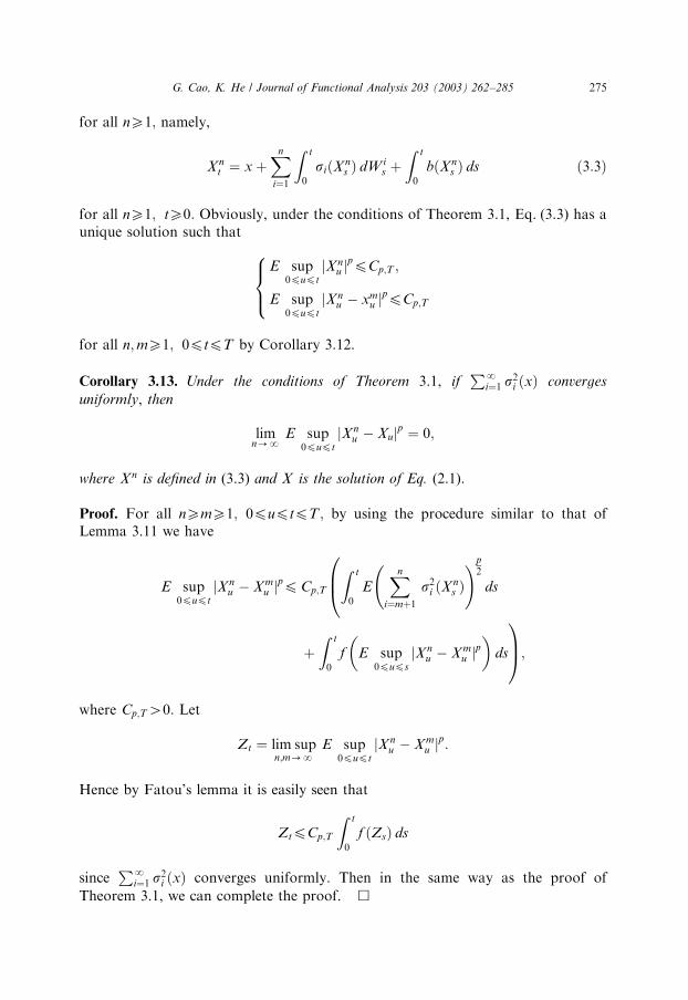
for all nX1; namely,

X nt ¼ x þ

Xn

i¼1

Z t

0

siðX ns Þ dW i

s þZ t

0

bðX ns Þ ds ð3:3Þ

for all nX1; tX0: Obviously, under the conditions of Theorem 3.1, Eq. (3.3) has aunique solution such that

E sup0pupt

jX nu j

ppCp;T ;

E sup0pupt

jX nu xm

u jppCp;T

8><>:

for all n;mX1; 0ptpT by Corollary 3.12.

Corollary 3.13. Under the conditions of Theorem 3.1, ifP

N

i¼1 s2i ðxÞ converges

uniformly, then

limn-N

E sup0pupt

jX nu Xujp ¼ 0;

where X n is defined in (3.3) and X is the solution of Eq. (2.1).

Proof. For all nXmX1; 0puptpT ; by using the procedure similar to that ofLemma 3.11 we have

E sup0pupt

jX nu X m

u jppCp;T

Z t

0

EXn

i¼mþ1s2i ðX n

s Þ !p

2

ds

0B@

þZ t

0

f E sup0pups

jX nu X m

u jp �

ds

1CA;

where Cp;T40: Let

Zt ¼ lim supn;m-N

E sup0pupt

jX nu X m

u jp:

Hence by Fatou’s lemma it is easily seen that

ZtpCp;T

Z t

0

f ðZsÞ ds

sinceP

N

i¼1 s2i ðxÞ converges uniformly. Then in the same way as the proof of

Theorem 3.1, we can complete the proof. &

ARTICLE IN PRESSG. Cao, K. He / Journal of Functional Analysis 203 (2003) 262–285 275

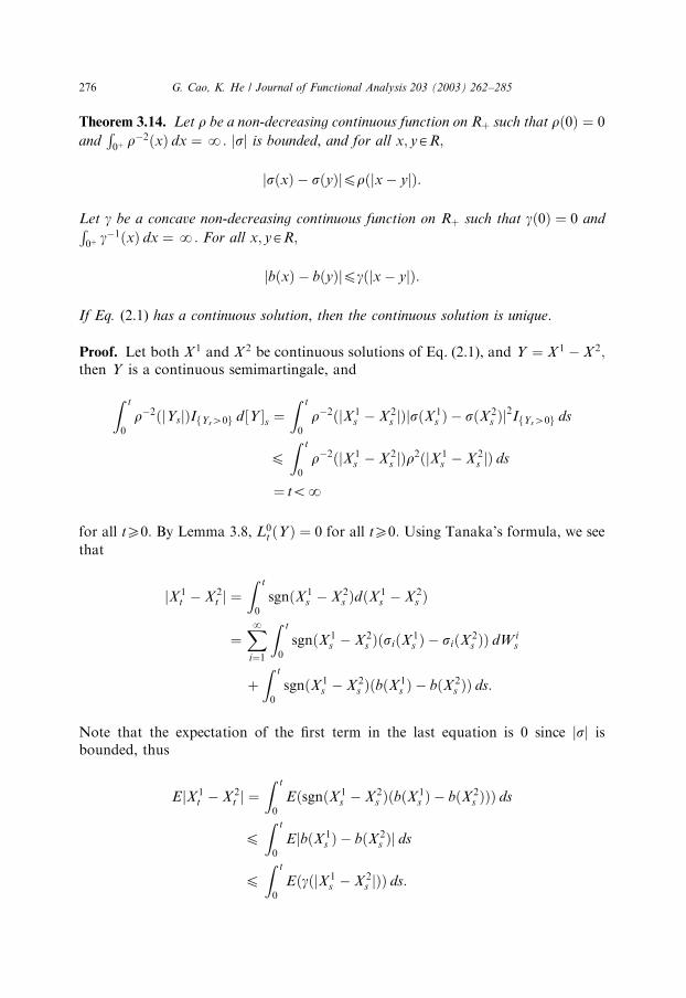
Theorem 3.14. Let r be a non-decreasing continuous function on Rþ such that rð0Þ ¼ 0

andR0þ r

2ðxÞ dx ¼ N: jsj is bounded, and for all x; yAR;

jsðxÞ sðyÞjprðjx yjÞ:

Let g be a concave non-decreasing continuous function on Rþ such that gð0Þ ¼ 0 andR0þ g

1ðxÞ dx ¼ N: For all x; yAR;

jbðxÞ bðyÞjpgðjx yjÞ:

If Eq. (2.1) has a continuous solution, then the continuous solution is unique.

Proof. Let both X 1 and X 2 be continuous solutions of Eq. (2.1), and Y ¼ X 1 X 2;then Y is a continuous semimartingale, and

Z t

0

r2ðjYsjÞIfYs40g d½Y �s ¼Z t

0

r2ðjX 1s X 2

s jÞjsðX 1s Þ sðX 2

s Þj2IfYs40g ds

pZ t

0

r2ðjX 1s X 2

s jÞr2ðjX 1s X 2

s jÞ ds

¼ toN

for all tX0: By Lemma 3.8, L0t ðYÞ ¼ 0 for all tX0: Using Tanaka’s formula, we see

that

jX 1t X 2

t j ¼Z t

0

sgnðX 1s X 2

s ÞdðX 1s X 2

s Þ

¼XNi¼1

Z t

0

sgnðX 1s X 2

s ÞðsiðX 1s Þ siðX 2

s ÞÞ dW is

þZ t

0

sgnðX 1s X 2

s ÞðbðX 1s Þ bðX 2

s ÞÞ ds:

Note that the expectation of the first term in the last equation is 0 since jsj isbounded, thus

EjX 1t X 2

t j ¼Z t

0

EðsgnðX 1s X 2

s ÞðbðX 1s Þ bðX 2

s ÞÞÞ ds

pZ t

0

EjbðX 1s Þ bðX 2

s Þj ds

pZ t

0

EðgðjX 1s X 2

s jÞÞ ds:

ARTICLE IN PRESSG. Cao, K. He / Journal of Functional Analysis 203 (2003) 262–285276

Hence by Jensen’s inequality,

EjX 1t X 2

t jpZ t

0

gðEjX 1s X 2

s jÞ ds:

Since t-EjX 1t X 2

t j is a non-negative continuous function on Rþ; one can apply

Lemma 3.7, and obtain

EjX 1t X 2

t j � 0

for all tX0; i.e. X 1t ¼ X 2

t for a.s. tX0: By using the procedure similar to that of the

proof of Theorem 3.1, the proof of the theorem is then complete. &

Remark. Let us take

r1ðxÞ ¼ Kxa;

where aX12; especially s satisfies Lipschitz condition when a ¼ 1; or let

r2ðxÞ ¼0; x ¼ 0;

Kðx log 1xÞ1=2; 0oxpd;

Kðd log 1dÞ1=2; x4d

8>><>>:

or take

r3ðxÞ ¼0; x ¼ 0;

Kðx log 1xlog log 1

xÞ1=2; 0oxpd;

Kðd log 1d log log

1dÞ1=2; x4d:

8>><>>:

And take

g1ðxÞ ¼ Kx;

i.e. b satisfies Lipschitz condition, or let

g2ðxÞ ¼0; x ¼ 0;

Kx log 1x; 0oxpd;

Kd log 1d; x4d

8><>:

or take

g3ðxÞ ¼0; x ¼ 0;

Kx log 1xlog log 1

x; 0oxpd;

Kd log 1d log log

1d; x4d;

8><>:

ARTICLE IN PRESSG. Cao, K. He / Journal of Functional Analysis 203 (2003) 262–285 277

where K40 and dAð0; 1Þ is sufficiently small. They all satisfy the conditions ofTheorem 3.14.

4. Non-contact property and strong comparison theorem

By using the method similar to the proof of Yamada–Ogura (cf. [13]), we can getthe following non-contact property and strong comparison theorem for solutions ofone-dimensional SDE.Let siðt; xÞ; bðt; xÞ; b1ðt; xÞ; b2ðt; xÞ be continuous functions Rþ � R-R; i ¼

1; 2; 3;y : Set

sðt; xÞ ¼ ðs1ðt; xÞ; s2ðt; xÞ;yÞ;

jsðt; xÞj ¼PNi¼1

s2i ðt; xÞ �1

2:

8>><>>:

Suppose sðt; xÞAl2 for all tX0; xAR:

Theorem 4.1 (Non-contact property). Let r be a non-decreasing continuous function

on Rþ such that rð0Þ ¼ 0 and

Z 1

0þ

Z 1

y

dx dy

r2ðxÞ ¼Z 1

0þ

x dx

r2ðxÞ ¼ N:

For all tX0; x; yAR;

jsðt; xÞ sðt; yÞjprðjx yjÞ:

Let g be a non-decreasing continuous function on Rþ such thatgð0Þ ¼ 0 and

limuk0

supupyp1

gðyÞZ 1

y

dx

r2ðxÞ

Z 1

u

Z 1

y

dx dy

r2ðxÞ

� !¼ 0:

For all tX0; x; yAR;

jbðt; xÞ bðt; yÞjpgðjx yjÞ:

Suppose we have two F0 measurable random variables x and Z; and twocontinuous semimartingales X ðt; xÞ and X ðt; ZÞ such that the following

ARTICLE IN PRESSG. Cao, K. He / Journal of Functional Analysis 203 (2003) 262–285278

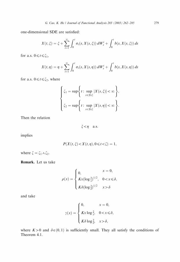
one-dimensional SDE are satisfied:

Xðt; xÞ ¼ xþXNi¼1

Z t

0

siðs;X ðs; xÞÞ dW is þ

Z t

0

bðs;Xðs; xÞÞ ds

for a.s. 0ptpz1;

Xðt; ZÞ ¼ ZþXNi¼1

Z t

0

siðs;X ðs; ZÞÞ dW is þ

Z t

0

bðs;Xðs; ZÞÞ ds

for a.s. 0ptpz2; where

z1 ¼ sup t : supsA½0;t�

jXðs; xÞjoN

( );

z2 ¼ sup t : supsA½0;t�

jXðs; ZÞjoN

( ):

8>>>>><>>>>>:

Then the relation

xoZ a:s:

implies

PðXðt; xÞoXðt; ZÞ; 0ptozÞ ¼ 1;

where z ¼ z14z2:

Remark. Let us take

rðxÞ ¼0;

x ¼ 0;

Kxðlog 2xÞ1=2; 0oxpd;

Kdðlog 2dÞ1=2

x4d

8>>><>>>:

and take

gðxÞ ¼

0; x ¼ 0;

Kx log 2x; 0oxpd;

Kd log 2d; x4d;

8>>><>>>:

where K40 and dAð0; 1Þ is sufficiently small. They all satisfy the conditions ofTheorem 4.1.

ARTICLE IN PRESSG. Cao, K. He / Journal of Functional Analysis 203 (2003) 262–285 279

Theorem 4.2 (Strong comparison theorem). Let r be a non-decreasing function on

Rþ such that rð0Þ ¼ 0 and Z 1

0þeeBðyÞ dy ¼ N

for any e40; where

BðyÞ ¼Z 1

y

dx

r2ðxÞ:

For all tX0; x; yAR;

jsðt; xÞ sðt; yÞjprðjx yjÞ:

Suppose

b1ðt; xÞob2ðt; xÞ

for all tX0; xAR; and X1ðt; xÞ;X2ðt; ZÞ are two continuous semimartingales suchthat the following one-dimensional SDE:

X1ðt; xÞ ¼ xþPNi¼1

R t

0 siðs;X1ðs; xÞÞ dW is þ

R t

0 b1ðs;X1ðs; xÞÞ ds;

X2ðt; ZÞ ¼ ZþPNi¼1

R t

0 siðs;X2ðs; ZÞÞ dW is þ

R t

0 b2ðs;X2ðs; ZÞÞ ds:

8>>>><>>>>:

Then the property

PðX1ðt; xÞpX2ðt; ZÞ; 0ptozÞ ¼ 1

implies

PðX1ðt; xÞoX2ðt; ZÞ; 0otozÞ ¼ 1;

where

z ¼ sup t : supsA½0;t�

jX1ðs; xÞjoN and supsA½0;t�

jX2ðs; ZÞjoN

( ):

Remark. Let us take

rðxÞ ¼ Kxa;

where K40 and 12oap1; especially s satisfies Lipschitz condition when a ¼ 1: It

satisfies the conditions of Theorem 4.2.

ARTICLE IN PRESSG. Cao, K. He / Journal of Functional Analysis 203 (2003) 262–285280

5. Example

Now we give an example which includes the equation for Brownian motion on thegroup of diffeomorphism of the circle (cf. [1,7] as a special case).Given

bðxÞ ¼ 0;

s1ðxÞ ¼ 0;

s2kþ1ðxÞ ¼ a2kþ1 sin kpx;

s2kðxÞ ¼ a2k cos kpx;

8>>><>>>:

where p40; a2k ¼ Oðkðpþ12ÞÞ; a2kþ1 ¼ Oðkðpþ1

2ÞÞ; k ¼ 1; 2; 3;y : We deduce

jsðxÞ sðyÞj2 ¼XNk¼1

ða22kðcos kpx cos kpyÞ2 þ a22kþ1ðsin kpx sin kpyÞ2Þ

pC0XNk¼1

kð2pþ1Þððcos kpx cos kpyÞ2 þ ðsin kpx sin kpyÞ2Þ

¼ 4C0XNk¼1

kð2pþ1Þ sin2kpðx yÞ

2¼ 4C0gðx yÞ;

where C040; gðxÞ ¼P

N

k¼1 kð2pþ1Þ sin2 kpx2: We see that the coefficients is non-

Lipschitz.

Theorem 5.1. Set

gðxÞ ¼XNk¼1

sin2 kpx2

k2pþ1 ;

where p40; then there exist a constant C40 such that

gðxÞpCx2 log1

jxj

for all x is sufficiently small.

Proof. The proof is borrowed from Airault–Ren, and we give it here in details forreader’s convenience.From the trapezoid formula,

1

2ðf ðaÞ þ f ða þ 1ÞÞ ¼

Z aþ1

a

f ðtÞ dt þZ aþ1

a

t a

2 ðt aÞ2

2

!f 00ðtÞ dt;

ARTICLE IN PRESSG. Cao, K. He / Journal of Functional Analysis 203 (2003) 262–285 281

we deduce

Xn

k¼1f ðkÞ ¼ 1

2f ð1Þ þ 1

2f ðnÞ þ

Z n

1

f ðtÞ dt þZ n

1

bðtÞf 00ðtÞ dt;

where bðtÞ ¼ t½t�2

ðt½t�Þ22

; ½t� denotes the integer part of t: Thus

gðxÞ ¼XNk¼1

sin2 kpx2

k2pþ1 ¼ 1

2sin2

x

2þZ

N

1

sin2 tpx2

t2pþ1 dt þZ

N

1

bðtÞlðtÞ dt;

where

lðtÞ ¼sin2 tpx

2

t2pþ1

!00

¼ p2x2 cos tpx

2t3 ð3p þ 3Þpx sin tpx

2tpþ3 þð2p þ 1Þð2p þ 2Þ sin2 tpx

2

t2pþ3 :

First we evaluate, for all 0oxo1ZN

1

bðtÞlðtÞ dt ¼ 1

px1=p

ZN

x

bt

x

� �1=p �

lt

x

� �1=p �

t1=p1 dt

¼ p2x2

4

ZN

1

2bðtÞt3

dt þ x2=pþ2

p

ZN

x

bt

x

� �1=p �

hðtÞ dt;

where

hðtÞ ¼ p2ðcos t 1Þ2t2=pþ1 ð3p þ 3Þp sin t

2t2=pþ2 þð2p þ 1Þð2p þ 2Þ sin2 t

2

t2=pþ3 ¼XNk¼0

ckt2k2=pþ1;

where ck is a constant for all kX1: The trapezoid formula applied to 1=t gives

Xn

k¼1

1

k¼ 1

2þ 1

2nþZ n

1

dt

tþZ n

1

2bðtÞt3

dt:

Thus ZN

1

2bðtÞt3

dt ¼ 12þ lim

n-N

Xn

k¼1

1

k log n

!¼ 1

2þ c;

where c is the Euler constant. Let

IðxÞ ¼Z

N

x

bt

x

� �1=p �

hðtÞ dt:

ARTICLE IN PRESSG. Cao, K. He / Journal of Functional Analysis 203 (2003) 262–285282

Note that 0pbðtÞp18for all tAR and jhðtÞjp p2

2t2=pþ1 þ ð3pþ3Þp2t2=pþ2 þ ð2pþ1Þð2pþ2Þ

t2=pþ3 for all t40;

then

jIðxÞjp1

8

ZN

x

jhðtÞj dtp1

8

Z 1

x

jhðtÞj dt þZ

N

1

jhðtÞj dt

�¼ Oðx2

pÞ:

Therefore ZN

1

bðtÞlðtÞ dt ¼ p2x2 18þ c

4

�þ x2=pþ2

pIðxÞ ¼ Oðx2Þ:

Next, we observe that for all 0oxo1;

ZN

1

sin2 tpx2

t2pþ1 dt ¼ x2

p

ZN

x

sin2 t2

t3dt ¼ x2

p

ZN

1

sin2 t2

t3dt þ

Z 1

x

sin2 t2

t3dt

!

¼ 1

4px2 log

1

x

�þ x2

p

ZN

1

sin2 t2

t3dt þ 1

2

Z 1

0

1 t2=2 cos t

t3dt

!

þ x2

2p

Z x

0

cos t 1þ t2=2

t3dt:

Since for the Euler constant c; we have

c ¼Z 1

0

1 cos t

tdt

ZN

1

cos t

tdt:

After two integration by parts, we findZN

1

sin2 t2

t3dt þ 1

2

Z 1

0

1 t2=2 cos t

t3dt ¼ 3

8 c

4:

On the other hand, we put

JðxÞ ¼ 1

2x2

Z x

0

cos t 1þ t2=2

t3dt ¼ 1

4

XNk¼0

ð1Þkx2k

ðk þ 1Þð2k þ 4Þ! ¼ Oð1Þ:

Therefore ZN

1

sin2 tpx2

t2pþ1 dt ¼ 1

4px2 log

1

x

�þ 3

8p c

4p

�x2 þ 1

px4JðxÞ

¼ 1

4px2 log

1

x

�þ Oðx2Þ:

ARTICLE IN PRESSG. Cao, K. He / Journal of Functional Analysis 203 (2003) 262–285 283

Thus for all 0oxo1;

gðxÞp 1

4px2 log

1

x

�þ Oðx2Þ ¼ O x2 log

1

x

� �:

The proof of the theorem is then complete. &

So we define

rðxÞ ¼0; x ¼ 0;

Kxðlog 1xÞ1=2; 0oxpd;

Kdðlog 1dÞ1=2; x4d;

8>><>>:

where K ¼ 2ffiffiffiffiffiffiffiffiffiC0C

p40 and dAð0; 1Þ is sufficiently small. It’s a concave non-

decreasing continuous function on Rþ; rð0Þ ¼ 0; andZ0þ

x dx

r2ðxÞ ¼ Z0þ

dx

K2x log x¼ 1

K2

Z0þ

d log x

log x¼ 1

K2logjlog xjj0þ ¼ N:

By Theorem 5.1 we have

jsðxÞ sðyÞjprðjx yjÞ;

i.e. rðxÞ satisfies the hypotheses of Theorem 3.1 at the case of p ¼ 2:

Acknowledgments

Both authors are very grateful to Professor Jiagang Ren for his encouragementand valuable discussions, and thank Dr. Jicheng Liu for his helpful suggestions andproviding us Ref. [6]. All of our remarks come from [3,5,8,9,12].

References

[1] H. Airault, J.G. Ren, Modulus of continuity of the canonic Brownian motion ‘‘on the group of

diffeomorphisms of the circle’’, J. Funct. Anal. 196 (2002) 395–426.

[2] G.L. Gong, An Introduction of Stochastic Differential Equations, 2nd Edition, Peking University

Press of China, Peking, 2000.

[3] Z.Y. Huang, Foundation of Stochastic Analysis, 2nd Edition, Science Press of China, Peking, 2001.

[4] J.F. Le Gall, Applications du temps local aux equations differentielles Stochastiques unidimension-

nelles. Sem. Prob. XVII. Lecture Notes in Mathematics, vol. 986. Springer-Verlag, Berlin/Heidelberg/

New York, 1983, pp. 15–31.

[5] Z.X. Liang, Existence and pathwise uniqueness of solutions for stochastic differential equations with

respect to martingales in the plane, Stochastic Process. Appl. 83 (1999) 303–317.

[6] J.C. Liu, On the existence and uniqueness of solutions to stochastic differential equations of mixed

Brownian and Poissonian sheet type, Stochastic Process. Appl. 94 (2001) 339–354.

ARTICLE IN PRESSG. Cao, K. He / Journal of Functional Analysis 203 (2003) 262–285284

[7] P. Malliavin, The canonic diffusion above the diffeomorphism group of the circle, C.R. Acad. Sci.

Paris, Ser. I t. 329 (1999) 325–329.

[8] X.R. Mao, Adapted solutions of backward stochastic differential equations with non-Lipschitz

coefficients, Stochastic Process. Appl. 58 (1995) 281–292.

[9] Z.K. Nie, Uniqueness on two-parameter Ito’s stochastic differential equations, Acta Math. Sinica. 30

(1987) 179–186.

[10] E. Perkins, Local time and pathwise uniqueness for stochastic differential equations, Sem. Prob. XVI.

Lecture Notes in Mathematics, vol. 920. Springer-Verlag, Berlin/Heidelberg, New York, 1982,

pp. 201–208.

[11] L.C.G. Rogers, D. Williams, Diffusions, Markov processes and Martingales, vol. 2, 2nd Edition,

Cambridge University Press, Cambridge, 2000.

[12] R. Situ, On solutions of backward stochastic differential equations with jumps and applications,

Stochastic Process. Appl. 66 (1997) 209–236.

[13] T. Yamada, Y. Ogura, On the strong comparison theorems for solutions of stochastic differential

equations, Z. Wahrscheinlichkeitstheorie Verw. Gebiete. 56 (1981) 3–19.

[14] T. Yamada, S. Watanabe, On the uniqueness of solutions of stochastic differential equations,

J. Math. Kyoto Univ. 11 (1971) 155–167.

ARTICLE IN PRESSG. Cao, K. He / Journal of Functional Analysis 203 (2003) 262–285 285