Investigation of Brownian Motion in Simple and Complex ...
235
Investigation of Brownian Motion in Simple and Complex Fluids under Oscillatory Perturbations Dissertation zur Erlangung des Grades des Doktors der Naturwissenschaften der Naturwissenschaftlich-Technischen Fakultät II - Physik und Mechatronik - der Universität des Saarlandes von Andreas Gross Saarbrücken 2014
-
Upload
khangminh22 -
Category
Documents
-
view
0 -
download
0
Transcript of Investigation of Brownian Motion in Simple and Complex ...

Investigation of Brownian Motion
in Simple and Complex Fluidsunder Oscillatory Perturbations
Dissertationzur Erlangung des Grades
des Doktors der Naturwissenschaftender Naturwissenschaftlich-Technischen Fakultät II
- Physik und Mechatronik -der Universität des Saarlandes
von
Andreas Gross
Saarbrücken
2014


Tag des Kolloquiums: 04.09.2014
Dekan: Univ.-Prof. Dr. rer. nat. Christian Wagner
Mitglieder des Prüfungsausschusses:
Vorsitzender: Univ.-Prof. Dr. rer. nat. Rolf Pelster
Gutacher: Univ.-Prof. Dr. rer. nat. Christian Wagner
Univ.-Prof. Dr. rer. nat. Albrecht Ott
Akad. Mitarbeiter: Dr. rer. nat. Andreas Tschöpe

iv
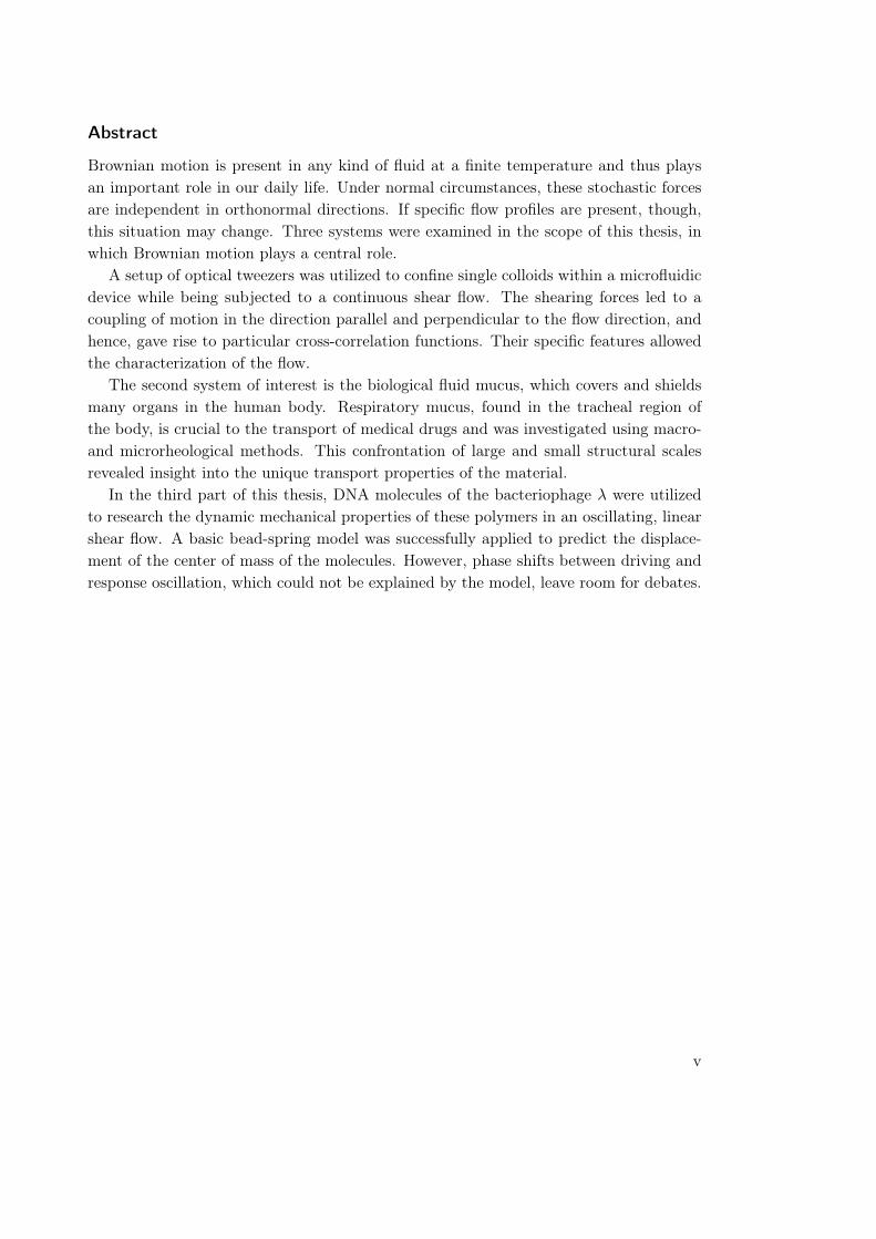
Abstract
Brownian motion is present in any kind of fluid at a finite temperature and thus playsan important role in our daily life. Under normal circumstances, these stochastic forcesare independent in orthonormal directions. If specific flow profiles are present, though,this situation may change. Three systems were examined in the scope of this thesis, inwhich Brownian motion plays a central role.
A setup of optical tweezers was utilized to confine single colloids within a microfluidicdevice while being subjected to a continuous shear flow. The shearing forces led to acoupling of motion in the direction parallel and perpendicular to the flow direction, andhence, gave rise to particular cross-correlation functions. Their specific features allowedthe characterization of the flow.
The second system of interest is the biological fluid mucus, which covers and shieldsmany organs in the human body. Respiratory mucus, found in the tracheal region ofthe body, is crucial to the transport of medical drugs and was investigated using macro-and microrheological methods. This confrontation of large and small structural scalesrevealed insight into the unique transport properties of the material.
In the third part of this thesis, DNA molecules of the bacteriophage λ were utilizedto research the dynamic mechanical properties of these polymers in an oscillating, linearshear flow. A basic bead-spring model was successfully applied to predict the displace-ment of the center of mass of the molecules. However, phase shifts between driving andresponse oscillation, which could not be explained by the model, leave room for debates.
v

Kurzzusammenfassung
In Flüssigkeiten laufen bei Temperaturen oberhalb des Nullpunkts jederzeit dynamischeProzesse ab, die durch die Brownsche Molekularbewegung verursacht werden. Normaler-weise ist die Bewegung in orthogonalen Richtungen statistisch unabhängig, in bestimmtenFlüssen kann sich diese Situation jedoch ändern. Im Rahmen dieser Dissertation wur-den drei Systeme untersucht, in denen der Brownschen Molekularbewegung eine zentraleBedeutung zukommt.
Eine optische Pinzette wurde verwendet um einzelne Kolloide in einer Mikrofluidikzu lokalisieren, während sie gleichzeitig einem kontinuierlichen Scherfluss ausgesetzt wur-den. Die Scherkräfte führten zu einer Kopplung der Auslenkungen in und senkrecht zurFlussrichtung und verursachten dadurch charakteristische Kreuzkorrelationsfunktionen.Ihr Verlauf konnte zur Analyse des Flusses eingesetzt werden.
Beim zweiten untersuchten System handelt es sich um Mukus, eine biologische Flüs-sigkeit, die viele Organe im menschlichen Körper bedeckt und schützt. RespiratorischerMukus, der im Bereich der Atemwege vorkommt, hat eine große Bedeutung beim Trans-port von Arzneiwirkstoffen in den Körper und wurde mittels makro- und mikrorheologis-cher Methoden untersucht. Die Gegenüberstellung der verschiedenen Größenordnungender Strukturen erlaubten Einblick in die einzigartigen Transporteigenschaften des Mate-rials.
Im dritten Teil der Arbeit wurden DNA der Bakteriophage λ verwendet, um ihredynamischen mechanischen Eigenschaften in einem oszillierenden, linearen Scherfluss zuerforschen. Ein grundlegendes Kugel-Feder-Modell wurde erfolgreich angewandt, umdie Auslenkung des Masseschwerpunktes der Moleküle vorherzusagen. Allerdings lassenPhasenverschiebungen zwischen antreibender Schwingung und Antwortschwingung, dienicht vom Modell erfasst werden konnten, Raum für Diskussion.
vi

Contents
Introduction 3
I. Investigation of Oscillatory Perturbations of a Colloid in LinearShear Flow 5
I.1. Introduction 7
I.2. Literature Survey 9
I.3. Optical Tweezers 13I.3.1. Historical Development . . . . . . . . . . . . . . . . . . . . . . . . . . . 13I.3.2. Scattering Regimes . . . . . . . . . . . . . . . . . . . . . . . . . . . . . 14
I.3.2.1. Rayleigh Regime . . . . . . . . . . . . . . . . . . . . . . . . . 14I.3.2.2. Ray Optics Regime . . . . . . . . . . . . . . . . . . . . . . . . 15I.3.2.3. Mie Regime . . . . . . . . . . . . . . . . . . . . . . . . . . . . 16
I.3.3. Force Balance Considerations . . . . . . . . . . . . . . . . . . . . . . . 17I.3.4. Summary . . . . . . . . . . . . . . . . . . . . . . . . . . . . . . . . . . . 18
I.4. Flows through Small Channels 19I.4.1. Solution of the Navier-Stokes Equation in Rectangular Channels . . 19I.4.2. Design of the Microfluidic Device . . . . . . . . . . . . . . . . . . . . . 23I.4.3. Colloids in Linear Shear Flow without Forced Oscillations . . . . . . 25I.4.4. Colloids in Linear Shear Flow Forced by an Oscillating Optical Trap 32I.4.5. Summary . . . . . . . . . . . . . . . . . . . . . . . . . . . . . . . . . . . 37
I.5. Numerical Analysis 39I.5.1. Colloids in a Quiescent Fluid . . . . . . . . . . . . . . . . . . . . . . . 40I.5.2. Colloids in Linear Shear Flow without Forced Oscillations . . . . . . 42I.5.3. Colloids in Linear Shear Flow Forced by an Oscillating Optical Trap 43I.5.4. Summary . . . . . . . . . . . . . . . . . . . . . . . . . . . . . . . . . . . 49
vii

Contents
I.6. Experimental Study 51I.6.1. Experimental Setup . . . . . . . . . . . . . . . . . . . . . . . . . . . . . 51
I.6.1.1. Guidance System of the Laser Beams . . . . . . . . . . . . . 52I.6.1.2. Microscope, Visualization, & Signal-Synchronization System 56I.6.1.3. Flow Control in the Microfluidic Device . . . . . . . . . . . . 60
I.6.2. Utilized Software . . . . . . . . . . . . . . . . . . . . . . . . . . . . . . . 61I.6.3. Calibration of the Setup . . . . . . . . . . . . . . . . . . . . . . . . . . 63I.6.4. Results . . . . . . . . . . . . . . . . . . . . . . . . . . . . . . . . . . . . . 70
I.6.4.1. Colloids in Linear Shear Flow without Forced Oscillations . 71I.6.4.2. Colloids in Linear Shear Flow Forced by an Oscillating Op-
tical Trap . . . . . . . . . . . . . . . . . . . . . . . . . . . . . . 76I.6.5. Summary . . . . . . . . . . . . . . . . . . . . . . . . . . . . . . . . . . . 84
I.7. Discussion 87
I.8. Summary 91
II. Macro- & Microrheology of Mucus 95
II.1. Introduction 97
II.2. Literature Survey 99
II.3. Rheology of Fluids 101II.3.1. Macrorheology . . . . . . . . . . . . . . . . . . . . . . . . . . . . . . . . 104II.3.2. Microrheology . . . . . . . . . . . . . . . . . . . . . . . . . . . . . . . . 106II.3.3. Summary . . . . . . . . . . . . . . . . . . . . . . . . . . . . . . . . . . . 109
II.4. Experimental Study 111II.4.1. Experimental Setups . . . . . . . . . . . . . . . . . . . . . . . . . . . . 111
II.4.1.1. Rheometer . . . . . . . . . . . . . . . . . . . . . . . . . . . . . 111II.4.1.2. Optical Tweezers . . . . . . . . . . . . . . . . . . . . . . . . . 112
II.4.2. Measurements . . . . . . . . . . . . . . . . . . . . . . . . . . . . . . . . 113II.4.2.1. Macrorheology . . . . . . . . . . . . . . . . . . . . . . . . . . . 113II.4.2.2. Microrheology . . . . . . . . . . . . . . . . . . . . . . . . . . . 119
II.4.3. Summary . . . . . . . . . . . . . . . . . . . . . . . . . . . . . . . . . . . 127
II.5. Discussion 129
II.6. Summary 135
viii

Contents
III. Single-End-Grafted DNA-Molecules in an Oscillatory Linear ShearFlow 137
III.1. Introduction 139
III.2. Literature Survey 141
III.3. Theory 145III.3.1. Flow Profile between Two Parallel Oscillating Surfaces . . . . . . . . 147III.3.2. Model for a Single-End-Grafted DNA-Molecule . . . . . . . . . . . . 150III.3.3. Summary . . . . . . . . . . . . . . . . . . . . . . . . . . . . . . . . . . . 154
III.4. Experimental Study 155III.4.1. Experimental Setup . . . . . . . . . . . . . . . . . . . . . . . . . . . . . 157III.4.2. Utilized Programs . . . . . . . . . . . . . . . . . . . . . . . . . . . . . . 161III.4.3. Measurements . . . . . . . . . . . . . . . . . . . . . . . . . . . . . . . . 163III.4.4. Summary . . . . . . . . . . . . . . . . . . . . . . . . . . . . . . . . . . . 172
III.5. Discussion 173
III.6. Summary 177
Summary 181
IV. Appendix 183
A. Materials & Methods 185A.1. Materials . . . . . . . . . . . . . . . . . . . . . . . . . . . . . . . . . . . 185A.2. Methods . . . . . . . . . . . . . . . . . . . . . . . . . . . . . . . . . . . . 186
A.2.1. Production of Microfluidic Devices . . . . . . . . . . . . . . . 186A.2.2. Preparation of Gene Frames for Microrheology Experiments 187A.2.3. DNA preparation . . . . . . . . . . . . . . . . . . . . . . . . . 187A.2.4. Preparation of a cover slip and DNA for shear experiments 188
B. Calculations 191B.1. Auto- and Cross-Correlation Functions of Brownian Motion in a
Shear Flow . . . . . . . . . . . . . . . . . . . . . . . . . . . . . . . . . . 191
C. Custom written Software 195C.1. Calculation of Auto- and Cross-Correlation Functions . . . . . . . . . 195
ix

Contents
D. Supplementary Tables 197
Acknowledgements 205
Eidesstattliche Versicherung 207
List of Variables 209
List of Figures 211
List of Tables 215
Bibliography 217
x

Introduction
1


The dynamics of Brownian suspensions are determined by the fluctuations of theirmicroscopic constituents. Even at rest or at equilibrium, one may observe a rich phasebehavior depending on properties like concentration, temperature, pressure, and manymore. In this context, it hence poses a very interesting challenge to evolve an under-standing of these phenomena. However, in most applications, fluids are typically not atrest but they flow in order to allow material transport. Thus, the study of fluids andthe Brownian fluctuations therein is important both for applications and from a scien-tific point of view. Here, one of the fundamental questions is: How will external fieldsinfluence and hence change Brownian dynamics?
The kind of systems which will be in the focus of this work contain sols and gels.In case of a sol, solid particles with sizes between 1 nm and approximately 10µm aredispersed in a continuous liquid phase (e. g. water, glycerol, etc). A gel, on the otherhand, is rather the opposite: Liquid “particles” are dispersed within a solid-like cross-linked network. In many cases, the network is built by polymers. Such materials, as theycontain both liquids and solids, thus also show both the elastic properties of a solid andthe viscous properties of a Newtonian fluid. This kind of a mixture of properties hencereveals rich characteristics which, due to their viscous and elastic nature, motivated theterm viscoelastic or also complex fluid for such materials. This class of materials is verycommon and often encountered in our everyday lives. We use them to bake a cake, i. e.the dough, to brush our teeth, they are contained within our food and so forth. We arecurrently just beginning to build an understanding of their material properties and, asalready mentioned, our grasp on Brownian dynamics within such materials is far frombeing complete. This is especially true as soon as external fields are involved and whenwe consider systems out of their thermodynamic equilibrium.
Within this thesis, the Brownian dynamic in oscillatory fields is studied for threedifferent experimental realizations. In part I, the motion of a colloid is examined in ashear flow while it is subjected to external oscillations. This is implemented by utilizinga setup of optical tweezers of which the main element is a strongly focused laser beam.It allows to confine particles to a small volume around the focal region of the beam andthus additionally enables the visualization of the particle’s motion over a long period oftime. A microfluidic device is used in combination with a gravitationally driven flow inorder to create the required shear flow. Such a shear flow provides a coupling of themotion of the colloid in perpendicular directions which would not be present in a systemin thermodynamic equilibrium. Thus, we expect the cross-correlation functions of themotion in these perpendicular directions to display characteristic properties which cannotbe found in the equilibrium system.Part II gives details about how external oscillatory driving of colloids can be used tostudy Brownian motion in complex environments like biological gels. In our case, thestudy was performed in mucus. The analysis of colloidal motion allows the determination
3

of the viscoelastic properties of the gel. In order to conduct this study, just as in case ofpart I, a setup of optical tweezers is utilized to confine and visualize the particles. Mucusis of specific interest in pharmaceutical research since it covers many cell surfaces withinthe human body and could be exploited for a more efficient drug transport. However,this is not possible without knowledge of the diffusion properties of colloids within thismaterial. Hence, in this study, we aim at the structural exploration of mucus by activeprobing with oscillating colloidal particles.In part III of this thesis, the simple case of a single particle in shear flow is extendedto long-chained polymers which are grafted to a surface while being subjected to anoscillating shear flow. When considering not only a single colloid but a whole chain ofparticles which are interlinked by springs, this represents a simple model for a polymer.As our polymer of choice we pick deoxyribonucleic acid (DNA) for this part of the study.The oscillating shear flow is created by aligning an optical lens, which is fixed to apiezoelectric device, in a certain distance above the plain surface the DNA is attached to.Oscillations are controlled through electric signals sent to the piezo device. By varyingthe distance between oscillating lens and the surface at rest as well as the oscillationamplitude and frequency we aim at gaining a deeper understanding of Brownian motionof polymers in shear flow.
4

Part I.
Investigation of OscillatoryPerturbations of a Colloid
in Linear Shear Flow
5


I.1. Introduction
This first part of the thesis deals with small particles of sizes in the micrometer range thatare immersed in the bulk of a fluid. Since all experiments discussed later will take placeat room temperature, among the first questions one should ask about such a system is:How exactly are the particles going to behave? What is going to happen if these particlesare driven out thermodynamic equilibrium by, say, an external flow?
To our current understanding, each fluid consists of molecules that move due to theirthermal energy. In doing so, since there is a great number of them, they cannot move farbefore encountering another molecule. When they approach each other closely enoughthey exchange momentum according to their angle of impact and their masses whichcauses their velocity and direction of propagation to change. Assuming a colloidal probeparticle in the bulk of a fluid which is bigger than the fluid molecules, these impacts comein from all directions, which means that in average the colloid just remains in its originalplace (Fig. I.1.1). However, Einstein could show that the particle diffuses randomly insuch a way that its mean squared displacements increase linearly in time. This is ofcourse only valid if the fluid container possesses no walls.
So after long years of discussion, the riddle of Brown’s molecular motion, which wasdiscovered in 1784, was finally solved about 120 years later in 1905. But even now inthe year of its 230th birthday, there are still many open questions in context with Brow-nian motion especially in non-equilibrium situations and it remains a much investigatedtopic. Colloidal suspensions like inks and paints play an important role in industrial
Figure I.1.1.: Arbitrary path (green) of a colloidal particle (red) in the bulk of a fluid (blue).
7

I.1. Introduction
applications. The equilibrium phase behavior of colloidal suspensions has been inten-sively studied, but still there is qualitative disagreement between theoretical predictionsand experimental results, even for thermodynamic phase transitions [1]. Recently, it wasfound that hydrodynamic interactions between colloids have to be considered even atequilibrium [2]. However, still one does not need to consider complex systems to findfascinating open questions. Even seemingly simple questions have not been answered yet:How will two or more colloidal particles in a fluid bath behave when they approach eachother? How will a confined colloid react when brought into a shear flow? Especially theexperimental examination of such systems has proven a challenge. One method whichenables the investigation and also the active manipulation of colloidal systems is a setupof optical tweezers. It was developed about 30 years ago by Arthur Ashkin [3] and im-proved further in the following years, so today it can be used efficiently in order to studycolloidal systems.
Part I of the thesis will focus on single particles immersed in water, which are confinedto a certain region within a microfluidic channel by optical tweezers. By choice of an opti-mal position close to the channel walls, the flow profile the particle interacts with is closeto a linear shear profile (Ch. I.4). Oscillatory motion of the trap position along the gradi-ent direction are used to drive the system even further out of equilibrium and by analysisof the auto- and cross-correlation functions the local shear rate can be determined. Thefeatures of these functions will be compared to earlier results gained by Andreas Ziehl[4, 5]. It is of great importance to understand how external forces like forced oscillationsinfluence confined colloids in a flow field. Especially, if and how these forces couple to theBrownian forces intrinsic to such systems and hence cause additional contributions to theauto- and cross-correlation functions of motion is an interesting question that was notfully answered in the past. If such contributions are indeed present they might also playa role for localized DNA molecules in shear flow as discussed in part III of this thesis.Thus, they should be understood first before more complex systems can be studied. Thefocus of this work will be threefold: In chapter I.4 a Langevin equation will be applied asthe constitutive differential equation of the system and solved analytically. Furthermore,the correlation functions of motion will be determined. Chapter I.5 deals with numericalsimulations that enable the examination of the behavior of the colloids not only underexperimental conditions but also under conditions that cannot be realized directly due torestrictions of the setup. The experimental study of the system is performed in chapterI.6. The results from all methods will be compared and discussed in chapter I.7.
8

I.2. Literature Survey
Brownian motion was in the scope of researchers since its discovery by Jan Ingenhouszin 1784 [6], who reported about coal dust moving on the surface of an alcohol droplet.These dust particles seemed to move back and forth in an irregular fashion without anyclear direction. The effect was forgotten for nearly half a century until Robert Brown,a Scotch biologist, rediscovered it for pollen on a water surface [7]. He assumed the lifeforce of the pollen as being responsible for this effect. The topic was covered in manya debate in the following years. As possible causes, heat, electricity, and light were themain suspects [8, 9].
Joseph Delsaulx was the first to suggest that the reason might be linked to fluidmolecules impacting on the surface of the immersed objects, which in turn leads to theirregular tumbling motion [10]. His suggestion was quite revolutionary since it containedthe idea that every fluid consists of smaller parts like molecules. It took until 1905 orrespectively 1906 when Albert Einstein [11] and Marian von Smoluchowski [12], indepen-dently from each other, formulated a theory to explain and prove the atomistic nature offluids. A quantitative proof was delivered a few years later by Jean-Baptiste Perrin [13],who managed to determine Avogadro’s or respectively Boltzmann’s constant experimen-tally. For this groundbreaking achievement, Perrin was honored with the Nobel prize in1926.
While Brownian motion was investigated during the 20th century using different meth-ods like light scattering [14] or the intensity analysis during fluorescence microscopy [15],experimental methods for the study of Brownian motion of colloids in active flows werescarce. When Arthur Ashkin demonstrated in 1986 how a focused laser beam couldbe used to confine and manipulate small particles [3], a very handy tool was developedwhich could be used to examine Brownian motion directly. Details about the historicalevolution of this technique and its applications will be given in the following chapterI.3. This chapter however will focus on the specific use of optical tweezers and similartechniques in context with correlation functions of Brownian motion in colloidal systemsthat was published until today.
The first study involving optical tweezers in the examination of cross-correlation-functions of Brownian motion of more than one colloid is published in a paper by Jens-Christian Meiners and Stephen Quake [16]. To achieve this, they used a dual-beamoptical tweezers setup to independently trap two particles. Each beam was visualizedon a separate quadrant photo diode after transiting through the sample cell to allow for
9

I.2. Literature Survey
Figure I.2.1.: Contributions of correlated and anti-correlated modes of motion of two beads along thesame coordinate axis. The decay time of correlated motion (black) is shorter than thedecay of the anti-correlated mode (red) and thus results in a minimum when adding bothcontributions up (blue).
the separate tracking of each bead. In their experiments, they placed both traps in closevicinity to each other on a line parallel to one of the main axes of their diodes, i. e. thex- or the y-axis. They showed experimentally that the auto-correlation functions of theposition in each direction of each bead was represented by a double exponential decayfunction. Much more remarkable however were their experimental results in respectto the bead-to-bead cross-correlation functions. When correlating the motion in the x-direction of the first bead (denoted by x1) with the motion of the second bead in the samedirection (denoted by x2), they found a dip in the cross-correlation function Cx1x2(τ)close to τ = 0 (compare to Fig. I.2.1). The same is true for the cross-correlations alongthe y-axis Cy1y2(τ)1. This dip originates from two superimposed exponential functions,one of which is related to the decay of correlated modes of motion (shown in black), whilethe second is related to the decay of anti-correlated modes of motion (shown in red).
A similar experiment was performed about 13 years later by Skryabina et al. [17]using magnetic microparticles. In comparison to the setup used by Meiners and Quake,this setup contained an electromagnet which allowed an additional magnetic manipula-tion of the beads. This again resulted in a shift of all the correlation functions. However,neither Meiners and Quake nor Skryabina et al. found any correlations for the motionin perpendicular directions, i. e. Cx1y1 = Cx2y2 = Cx1y2 = Cx2y1 = 0. Since Brownianfluctuations in isotropic systems at equilibrium occur due to collisions with surround-ing molecules in an arbitrary way and hence the motion in perpendicular directions is
1For the sake of brevity, the time-dependence of the correlation functions is omitted in the rest of thischapter although the fluctuations are still time-dependent.
10
completely uncorrelated this result is not surprising. However, it is possible to observenon-zero cross-correlations of Brownian motion as soon as a coupling mechanism for per-pendicular directions is introduced into the system as for example a shear flow. This wasobserved by Ziehl et al. in experiments [5] and by Bammert et al. [18] as well as Holzeret al. [19] in theory. Instead of immersing the particles in a quiescent fluid withoutany kind of flow, Ziehl placed the particles in the middle of a microfluidic counter-flowdevice. While the particles experienced nearly no absolute flow velocity, they were at thesame time positioned in the region of the strongest shear gradient. The shear flow led tothe coupling of motion in perpendicular directions, so additional cross-correlations werefound.
Experiments and theory agree on the results for one single and two particles in shearflow. While the auto-correlation functions remain unchanged for a single particle, theshear flow causes the cross-correlation function Cxy to deviate from zero (this case will bediscussed in more detail in chapter I.4.3). The most interesting feature is the asymmetryof the function in respect to time which results from the bead being driven out of itsthermodynamic equilibrium by the flow. In case of two beads in close vicinity to eachother, this effect adds up with the hydrodynamic interaction, so even the movement ofthe first bead along the x-axis is coupled with the movement of the second bead alongthe y-axis, i. e. Cx1y2 ≠ 0. This can be explained in the following way: Both beadsinteract hydrodynamically causing an anti-correlation of Cx1x2 as discovered by Meinersand Quake. Due to the shear flow, Cxiyi shows correlations for each of the beads as well.This information is carried over to the other bead through hydrodynamic interactioncausing Cxiyj (i ≠ j) to be coupled. In addition to the case of both beads being placed onthe same streamline, Bammert also discusses the situation when both beads are placedabove and below the center streamline in the same distance from it. He furthermoretakes oblique cases into account.
Apart from these five publications there have been more publications in the field ofcross-correlations in context with the study of Brownian motion in flows. Many of themare only related indirectly and deal with the application of particle image velocimetry inmicrochannels [20, 21, 22]. There has also been a report on the usage of temperature-related broadening of correlation peaks in temperature measurements within fluid cells[23]. Correlation functions have also been used to detect the torque of particles that wereconfined within an optical trap [24]. In this study, we apply an additional oscillation tothe base shear flow used by A. Ziehl [5]. In this manner, we introduce a further timescale into the system which may give access to fascinating dynamics of colloids away fromthermodynamic equilibrium. The study of Brownian motion in an oscillatory shear flowis of great importance since it is a common situation. Consider for example the pulsatingflow of blood which can be described by a continuous shear flow with an additionaloscillatory contribution. Also the results will help in understanding the influence of theshear flow on DNA molecules which are grafted to one of the side walls of a flow chamber.
11

I.2. Literature Survey
Hence, the pre-requisites for the analysis of the dynamics of DNA molecules in oscillatingshear flows in part III of this work will be achieved in this first part.
The first part of this thesis is going to focus on a special implementation of the last ofthese questions. Specifically, the position of the optical trap will oscillate harmonicallyin the direction perpendicular to the flow direction in the microchannel while a bead isconfined in it. Similar to the state in the counter-flow device of Andreas Ziehl, the shearflow will cause a non-equilibrium situation for the bead which is additionally perturbedby the oscillatory motion of the trap.
12
I.3. Optical Tweezers
I.3.1. Historical Development
Light or electromagnetic radiation can be described as a wave and as a particle at thesame time. This principle, which is well-known as wave-particle dualism, was found byAlbert Einstein as the explanation for the photoelectric effect and published in one ofhis famous papers from 1905 [25]. It was the first quantum-physical explanation thatconsidered light as a quasi-particle called photon that is able to interact with matter.Thus, the effect that an electric current is caused by light shining on a surface can beunderstood. But even hundreds of years before, when Johannes Kepler watched thepassage of comet Halley, he detected that the tail of the comet was directed away fromthe sun. He explained this effect by the radiation pressure of the sun. Today, applicationsfor radiation pressure exist over a wide scale of sizes. Among the largest are solar sailswhich are used for the propulsion of satellites, among the smallest are optical tweezers.
The first realization of a setup of optical tweezers was developed by Arthur Ashkinin 1970 [26] and used two counter-propagating laser beams to confine particles. Whilecreating stable traps, this kind of a setup brought the disadvantage that either two lasershad to be used or the beam of a single laser had to be split and carefully aligned. Still,it presented the proof-of-principle that it is possible to confine particles by light. In thefollowing years, Ashkin continued his work on optimizing his setup which led amongothers to a levitation trap [27] and finally, about 15 years later, to the typical setup as itis still used today [3]. Only a single, tightly focused beam is used, which is thus able todirectly confine particles. Ashkin also worked on a theoretical model for the interactionof the laser with the particles [28, 29, 30].
Since then, a wide range of applications has been found for optical tweezers in scien-tific research. One of the most famous is the use for force measurements at molecularmotors [31, 32, 33] and DNA molecules [34, 35]. Also in recent years, microrheologybecame more important, which was established by Mason in 1995 [36] and used for theexamination of numerous fluids like polymers [37, 38], gels [39, 40], and especially bi-ological materials like the filamentous bacteriophage fd [41], B lymphocyte membranetethers [42], fibroblast cells [43], and more. The huge advantage of microrheology in thiscontext is two-fold. On the one hand, no mechanical contact with the sample is neces-sary to perform measurements and manipulate particles, which reduces the probabilityof contamination. On the other hand, measurements can be performed in the smallest
13

I.3. Optical Tweezers
sample volumes, even smaller than 30µl.The following chapter will give details on the interaction of laser light in a setup of
optical tweezers with small particles by scattering. It will conclude with the derivation ofa simple interaction force which will be used in the analytical examination of the systemlater.
I.3.2. Scattering Regimes
A setup of optical tweezers will play a central role in this part and also part II about therheology of mucus. Thus, developing an understanding of its basic properties is importantfor the discussions following later. While details about the construction of such a setupwill follow in chapter II.4, here, the electromagnetic interaction of the involved laserswith colloids will be explained. They will play a crucial role in the analytic description ofthe system and the equations of motion of the particles in the focal region of an opticaltrap.
When considering scattering of photons by colloids in a setup of optical tweezers,the interaction of light and colloid can be split into a force that stabilizes the trap, alsocalled gradient force, and a second one that decreases its stability, the so-called scatteringforce. The models that qualify to describe their interaction depend on the relation ofthe wavelength of the photon to the size of the colloid dc = 2rc , where rc is the radiusof the colloidal particle. The following sections deal with three size regimes that resultfrom this comparison.
I.3.2.1. Rayleigh Regime
The first case considered here deals with colloid sizes much smaller than the wavelength ofthe laser beam (dc ≪ λ). Due to their small size, colloids can be described as punctiformelectric dipoles interacting with the electric field component of the light [44]. This idearesults in two formulas for the scattering and gradient force [3]
Fscat =σsnmc
⟨S⟩ , (I.3.1)
Fgrad =αp
2∇ ⟨E2⟩ . (I.3.2)
Here, the scattering cross-section is given as
σs =128π5r6
c
3λ4(m
2r − 1
m2r + 2
)2
(I.3.3)
14

I.3.2. Scattering Regimes
and αp represents the polarizability of the colloid
αp = n2mr
3c (m2r − 1
m2r + 2
) . (I.3.4)
In these formulas, the optical properties of the colloids and the surrounding mediumare contained in the shape of the respective refractive indices nc and nm as well as therelative refractive index mr = nc/nm .
I.3.2.2. Ray Optics Regime
If the particle size is big in comparison to the wavelength of the laser (dc ≫ λ), theinteraction of light and matter can be described by classical ray optics. This meansthat the laser is divided into infinitely small partial beams that move in straight pathsuntil they reach an interface to a material with different optical properties. Under theassumption that there is no partial reflection of the incoming beam, the rays propagateaccording to Snell’s law [44]
nm sin (θi) = nc sin (θe) . (I.3.5)
Here, nm and nc denote the refractive indices of medium and colloid, θi and θe representthe angle of incidence and emergence of the beam relative to the surface normal vector.
Figure I.3.1.: The quality factors for scattering (Eq. I.3.6) and gradient force (Eq. I.3.7) are plottedhere for incidence angles between 0○ and 90○. A combination of water as the surroundingmedium (nm ≈ 1.33) and polymethylmethacrylate (PMMA) as the colloid material (nc ≈
1.49) was assumed for the calculation.
15

I.3. Optical Tweezers
However, partial transmission and reflection of the beams must also be taken intoaccount. Here, every time a ray of power P encounters an interface, only a part of it isable to transmit, while the rest is reflected at the interface. When integrating over thewhole width of the incoming laser beam, one can define the total scattering and gradientforces as [30]
∣Fscat∣ =nmP
c[1 +RF cos (2θi) −
T 2F (cos (2θi − 2θe) +RF cos (2θi))
1 +R2F + 2RF cos (2θe)
]
´¹¹¹¹¹¹¹¹¹¹¹¹¹¹¹¹¹¹¹¹¹¹¹¹¹¹¹¹¹¹¹¹¹¹¹¹¹¹¹¹¹¹¹¹¹¹¹¹¹¹¹¹¹¹¹¹¹¹¹¹¹¹¹¹¹¹¹¹¹¹¹¹¹¹¹¹¹¹¹¹¹¹¹¹¹¹¹¹¹¹¹¹¹¹¹¹¹¹¹¹¹¹¹¹¹¹¹¹¹¹¹¹¹¹¹¹¹¹¹¹¹¹¹¹¹¹¹¹¹¹¹¹¹¹¹¹¹¹¹¹¹¹¹¹¹¹¹¹¹¹¹¹¹¹¹¹¹¹¹¹¹¹¹¹¹¹¹¹¹¹¹¹¹¹¹¹¹¹¹¹¹¹¹¹¹¹¹¹¹¹¹¸¹¹¹¹¹¹¹¹¹¹¹¹¹¹¹¹¹¹¹¹¹¹¹¹¹¹¹¹¹¹¹¹¹¹¹¹¹¹¹¹¹¹¹¹¹¹¹¹¹¹¹¹¹¹¹¹¹¹¹¹¹¹¹¹¹¹¹¹¹¹¹¹¹¹¹¹¹¹¹¹¹¹¹¹¹¹¹¹¹¹¹¹¹¹¹¹¹¹¹¹¹¹¹¹¹¹¹¹¹¹¹¹¹¹¹¹¹¹¹¹¹¹¹¹¹¹¹¹¹¹¹¹¹¹¹¹¹¹¹¹¹¹¹¹¹¹¹¹¹¹¹¹¹¹¹¹¹¹¹¹¹¹¹¹¹¹¹¹¹¹¹¹¹¹¹¹¹¹¹¹¹¹¹¹¹¹¹¹¹¹¹¶Qscat
, (I.3.6)
∣Fgrad∣ =nmP
c[RF sin (2θi) −
T 2F (sin (2θi − 2θe) +RF sin (2θi))
1 +R2F + 2RF cos (2θe)
]
´¹¹¹¹¹¹¹¹¹¹¹¹¹¹¹¹¹¹¹¹¹¹¹¹¹¹¹¹¹¹¹¹¹¹¹¹¹¹¹¹¹¹¹¹¹¹¹¹¹¹¹¹¹¹¹¹¹¹¹¹¹¹¹¹¹¹¹¹¹¹¹¹¹¹¹¹¹¹¹¹¹¹¹¹¹¹¹¹¹¹¹¹¹¹¹¹¹¹¹¹¹¹¹¹¹¹¹¹¹¹¹¹¹¹¹¹¹¹¹¹¹¹¹¹¹¹¹¹¹¹¹¹¹¹¹¹¹¹¹¹¹¹¹¹¹¹¹¹¹¹¹¹¹¹¹¹¹¹¹¹¹¹¹¹¹¹¹¹¹¹¹¹¹¹¸¹¹¹¹¹¹¹¹¹¹¹¹¹¹¹¹¹¹¹¹¹¹¹¹¹¹¹¹¹¹¹¹¹¹¹¹¹¹¹¹¹¹¹¹¹¹¹¹¹¹¹¹¹¹¹¹¹¹¹¹¹¹¹¹¹¹¹¹¹¹¹¹¹¹¹¹¹¹¹¹¹¹¹¹¹¹¹¹¹¹¹¹¹¹¹¹¹¹¹¹¹¹¹¹¹¹¹¹¹¹¹¹¹¹¹¹¹¹¹¹¹¹¹¹¹¹¹¹¹¹¹¹¹¹¹¹¹¹¹¹¹¹¹¹¹¹¹¹¹¹¹¹¹¹¹¹¹¹¹¹¹¹¹¹¹¹¹¹¹¹¹¹¹¹¹¶Qgrad
, (I.3.7)
where RF and TF are Fresnel’s coefficients of reflection or, respectively, transmission.The terms in brackets are denoted as the quality factors of scattering and gradient forceQscat and Qgrad . These allow the determination of the ideal angle of incidence for a givencombination of medium and colloid materials (compare Fig. I.3.1). The graph displaysthe quality factors for the combination of polymethylmethacrylate (PMMA) beads inwater, the most common materials used in this part of the thesis. The highest value ofthe gradient quality factor is reached at about 72○, while the scattering is strongest around82○. This leads to the conclusion that the optimal angle of incidence lies around 50○−70○
where a high absolute value of Qgrad is reached, while the relative value Qgrad/Qscat is asbig as possible. Such high angles of incidence can only be realized by an objective of highnumerical aperture. A stable confinement of a particle is possible only if the surroundingmedium is of less optical density than the sphere, i. e. nc > nm. If this was the case, thesphere would always be pushed away from the focal point and stable trapping would beimpossible.
I.3.2.3. Mie Regime
In this intermediate regime in which the wavelength of the light is of roughly the sameorder as the particle size (dc ≈ λ), additional corrections to the forces of the Rayleighregime have to be taken into account. This can either be attempted by using an approachvia the coupled-dipole method [45] or the generalized Lorenz-Mie theory (GLMT) [46, 47].To achieve a more precise formulation of the acting forces, the plane of polarization of thelaser beam itself also has to be taken into account [48]. More details on the description ofscattering in the Mie regime can as well be found in a book by Bohren and Huffman onthe absorption and scattering of light by small particles [44]. Due to its large complexity,this regime will not be discussed in the scope of this thesis. However, more details aboutit can be found by the attentive reader in the referenced literature.
16

I.3.3. Force Balance Considerations
I.3.3. Force Balance Considerations
As becomes apparent depending on the size of the scattering object as compared tothe wavelength of light different descriptions of the interaction of light and matter areapplicable. No matter which scattering regime is considered there are always two commonforces (Fig. I.3.2): A scattering force Fscat pushes the sphere in direction of the Poyntingvector of the incident beam and a gradient force Fgrad pulls the sphere in direction of thestrongest electric field gradient. If a focused beam is assumed at this point as indicated infigure I.3.2 the sphere moves towards the focal point of the laser. However, the scatteringforce results in the sphere always being pushed slightly away from the focal point so thatit reaches a new equilibrium position. In total, close to the focal point of the laser beam,all acting forces can be combined to a linear law independent of the size regime
Ftrap = −ktrap∆r , (I.3.8)
where ∆r denotes the displacement of the trapped object away from the focal point. Thespring constant or trap stiffness ktrap can vary from one Cartesian direction to another,in general, the components are identical. However, equation I.3.8 only holds true closeto the focal point of the laser. For bigger distances, higher order corrections have to betaken into account.
Figure I.3.2.: Total force balance of scattering and gradient force for the interaction of a focused laserbeam with a sphere of refractive index nc in a medium of index nm. Two exemplaryincident beams Ai and Bi are partially reflected (Ar and Br) and partially transmittedthrough the sphere (At and Bt). Multiple reflections within the sphere are not depictedto keep the image clear. The colored bar on the left side of the sketch indicates theGaussian intensity distribution of the laser beam.
17

I.3. Optical Tweezers
I.3.4. Summary
In the past chapter, the principle of optical tweezers was discussed. The main feature isa strongly focused laser beam that interacts with objects in its beam path. The exactdescription of this interaction depends on the size of the object relative to the wavelengthof the beam. Small objects (dc ≪ λ) act as punctiform dipoles in the electromagneticfield of the laser [3], while bigger objects (dc ≫ λ) lead to classical refraction of the beam[30]. For all regimes, acting forces can be sub-divided into a scattering force Fscat anda gradient force Fgrad. While Fscat always leads to a weakening of the trap since it isdirected in the propagation direction of the laser beam, Fgrad stabilizes the trap if thesetup of optical tweezers is constructed correctly. The total force acting on a sphere in anoptical trap is described by a linear law (Eq. I.3.8) which will be helpful in the followingchapters to derive a differential equation of motion for the confined particle. This forcebalance in context with the scattering and gradient forces will have repercussions on theactual construction of the setup utilized in this study. More details on this topic willfollow in a later chapter (Sect. I.6.1).
18
I.4. Flows through Small Channels
In this thesis, microfluidic channels are used to create a shear flow. They are designatedmicrofluidic devices since at least one of their dimensions is in the micrometer range.This is certainly the case here, since they have a width of 50µm and a height of about40µm. While the flow is purely gravitationally driven, which results in a Poiseuillevelocity profile, these kinds of devices can be used to create quasi-linear shear flows,nonetheless. This idea will be developed over the course of the next sections.
The second topic and one of the central keypoints of this thesis is the interactionof a trapped colloid with the flowing fluid. The force balance for such a bead will bediscussed without (Sect. I.4.3) and with forced oscillations (Sect. I.4.4), and the solutionsof the differential equations will be employed to determine the auto- and cross-correlationfunctions of their motion.
I.4.1. Solution of the Navier-Stokes Equation in RectangularChannels
When talking about microfluidic devices and flows through channels, among the firstquestions asked should be how the velocity profile of the fluid will look like. Centralprinciples necessary for the solution are the conservation of mass, momentum, and energy[49]. Then, the Navier-Stokes equation can be cast in the following form
ρ( ∂∂t
+ v∇) v = η∆v − ∇p + ρg , (I.4.1)
where p is the pressure, ρ the density, and η the dynamic viscosity of the fluid. This equa-tion gives the full Navier-Stokes equation with which any kind of flow in any geometrycan be characterized. For steady unidirectional flows like present in a rectangular channeldriven by hydrostatic pressure, this problem can be strongly simplified. Then, the flowcan be considered stationary, eliminating the time-dependence, and also convection-free.The description can be reduced to the Stokes equation
η∆v − ∇p + ρg = 0 (I.4.2)
19

I.4. Flows through Small Channels
Figure I.4.1.: Color-coded plot of the normalized flow velocity in the x-direction of a rectangular chan-nel in the y-z-plane. The velocity increases from a complete stand-still at the channelwalls (dark blue) to the maximum velocity in the center of the channel (red). The whitehorizontal line indicates the cutting line along which the flow profile in Fig. I.4.2 isdrawn.
or respectively when assuming a channel with a flow solely in the horizontal x-directionof velocity vx ≙ v
η ( ∂
∂y2+ ∂
∂z2) v − ∂p
∂x= 0 . (I.4.3)
A solution can be computed for no-slip boundary conditions1 by using Fourier-expansionsin the z-direction, giving [50]
v(y, z) = 3Q
8ab3F (ab)
⎡⎢⎢⎢⎣b2 − z2 + 4b2
∞
∑n=1
(−1)n
α3n
cosh (αn yb )cosh (αn ab )
cos(αnz
b)⎤⎥⎥⎥⎦, (I.4.4)
where Q is the flow rate, a is half the channel width, b is half of its height, αn =(2n − 1)π/2, and
F (x) = 1 − 6
x
∞
∑n=1
tanh (αnx)α5n
. (I.4.5)
1When assuming no-slip boundary conditions, the velocity of the fluid at the position of the containerwalls equals the velocity of the walls themselves. Here, the walls do not move at all leading to theconditions v(y = −b/2) = v(y = +b/2) = v(z = −a/2) = v(z = +a/2) = 0.
20

I.4.1. Solution of the Navier-Stokes Equation in Rectangular Channels
(a) Full-width profile. (b) Zoom of the region close to the wall.
Figure I.4.2.: Plot of the normalized flow velocity v against the position y at a fixed height z = 0µmin the middle of the channel as indicated by the white line in Fig. I.4.1. While thecomputed profiles are shown in black, a linear fit to the data close to the wall is shownin red.
In this case, the origin is placed in the middle of the channel. A color-coded plot in they-z-plane of a rectangular channel is drawn in Fig. I.4.1. Since all the experiments wereperformed close to the center-line in respect to the height of the channel at z = 0µm,a two-dimensional profile along that line is displayed in Fig. I.4.2. While the full pro-file shows the characteristic parabolic shape (Fig. I.4.2a) typical for a Poiseuille-typepressure-driven flow, in close proximity of the wall the velocity increases nearly linearlywith the distance y to the wall (Fig. I.4.2b). It appears reasonable to assume a linearshear profile for the distances used in the experiments introduced later in chapter I.6,which lie in a range of 2 to 4 times the particle radius corresponding to 4µm to 8µm.Especially, one has to take into account that only a small region around the averageposition of the oscillating optical trap will be visited by the confined beads; the typicalamplitude amounts to 1µm. At the same time however, the bead in the optical trapshould be as close as possible to the center of the channel in z-direction, because oth-erwise there might exist an additional shear gradient in this direction which cannot bemonitored directly. An evaluation of the height of the bead is not established in thecurrent setup.
In context with flows through small channels, a further topic shall be discussed: thelaminarity of the flow. Usually, the Reynolds number is evaluated as a means to char-acterize the flow in this respect. It weighs the inertial forces active in the flowing fluidagainst the viscous ones. It is a dimensionless number and as such gives an indicationwhether a flow tends to be laminar - this is the case when the viscous forces dominateover the inertial ones - or turbulent depending on its magnitude. In general, it is defined
21

I.4. Flows through Small Channels
as
Re = ρvdhη
, (I.4.6)
where dh is the hydraulic diameter of the channel and v the average flow velocity. Sincethe Reynolds number was originally defined for pipes with a round cross-section, a cor-rection has to be included, if channels with a different cross-section, i. e. rectangularones, are utilized. It can be determined as
dh = 4A
P= 2wh
w + h, (I.4.7)
where A is the area of the cross-section of the channel and P is its wetted perimeter. Theright-hand side of the equation shows the corresponding result for the chosen channel,where w is its width and h its height. This gives the adapted Reynolds number for arectangular channel
Rerectangular =2ρvwh
η (w + h)≈ 0.004 . (I.4.8)
The typical maximum velocity of the flows applied in this part of this doctoral researchstudy lies at 100µm/s and since all experiments were performed in water, the densityρ = 1000kg/m3 and viscosity η = 10−3 Pas of water were used. For the estimation, cor-responding to the experiments detailed later a channel width of 50µm and a height of40µm were assumed. As far as critical Reynolds numbers are concerned, there is no gen-eral number that is valid for all geometries and systems. If the Reynolds number is muchsmaller than 1, the physical system can be considered as behaving purely laminar. WithRerectangular in the order of magnitude between 10−3 to 10−2, any turbulence will decayfaster than the temporal resolution of the measurement and will only have a marginalinfluence on the flows.
One important correction has to be taken into account when handling beads very closeto side walls of channels: These beads will behave as if moving in a fluid of higher viscositythe closer they approach the wall. This effect is caused by hydrodynamic interaction ofthe spheres with the walls. It only applies for motion along the surface normal of thewall while motion perpendicular to it is not influenced at all. Assuming that a colloidapproaches a wall, the fluid in-between has to be pushed out before the colloid can moveany closer. This requires more force as compared to motion in the bulk of the fluid, thus,the effective viscosity for motion towards the walls seems higher. Of course, the actualviscosity of the fluid remains unchanged, the effect is just a pretended effect through theinteraction of colloid and wall. The viscosity increase can be computed by using Faxén’s
22

I.4.2. Design of the Microfluidic Device
law [51]
ηeff = η0 (1 − 9
16
rcdcw
+ 1
8( rcdcw
)3
− 45
256( rcdcw
)4
− 1
16( rcdcw
)5
)−1
, (I.4.9)
where ηeff is the effective viscosity, η0 is the bulk viscosity of the fluid, rc is the radius ofthe colloid, and dcw is the distance of the center of the colloid to the wall. When only thefirst order correction is taken into account, this leads to a viscosity increase of roughly25% for dcw = 3rc. Although a viscosity change of this order is quite significant, thisis the smallest distance chosen in the experiments presented in later chapters and canthus be seen as an upper limit. Since the viscosity has to be known for the calibrationof the trap stiffness as well, it will be influenced implicitly (Sect. I.6.3). To avoid theseinfluences by the walls becoming too strong, only those measurements will be consideredwhere the trap stiffnesses parallel and perpendicular to the walls do not differ from eachother by more than 10%.
I.4.2. Design of the Microfluidic Device
The main goal of this first part of the dissertation is the visualization of the motion ofparticles confined in an oscillating optical trap while exposed to a linear shear flow. Ameans to create a flow which can be approximated locally as a shear flow is given by amicrofluidic device with channels of rectangular cross-section, as discussed in the pastsection. If the bead is placed close to the center in z-direction and at the same timeclose to one of the side walls of the channel in y-direction, the conditions are close toideal (compare Fig. I.4.2). However, the techniques necessary to build such a devicehave to make dimensions in the order of 10µm possible. So-called soft lithographytechniques [52] are a very convenient way of fabrication. A particular one amongst thesemethods is designated as replica molding. First, a mold is necessary which carries thenegative structures of the desirable geometry. It is then filled with a soft material like
Figure I.4.3.: Example of a mask used for lithographic processing of silicon wafers in manufacturingthe mold for soft lithography. The patterns shown here represent a channel width of200µm and a length of 2 cm. For the experiments, only channels with a width of 50µmwere used.
23

I.4. Flows through Small Channels
Figure I.4.4.: This photograph shows a fully prepared microfluidic device after bonding to a roundcoverslide and tubes having been inserted as in- and outlets for a fluid.
polydimethylsiloxane (PDMS), which gives the positive counter-structure to the mold.After curing, the PDMS hardens and can be used for example for the realization ofmicrochannels. To avoid the evaporation of sample fluid and also dust particles in thesystem during an experiment, the channels should be closed off by using coverslides.Details on the production of the microfluidic devices using this method can be found inthe “Methods” section of the appendix (Sect. A.2.1).
The production of the mold can also be achieved using a multitude of techniques.If the size of the structures ranges in the order of magnitude of millimeters or bigger,a mold can be manufactured using mechanical methods like the milling of metal. Forsmaller molds on the micrometer scale, the manufacturing can be achieved by lithographytechniques on silicon. For that purpose, patterns on a mask are transferred by exposingthem to light into a photo resist, followed by the removal of either the exposed or thenon-exposed structures depending on the type of resist. The remainder of this procedurecan finally be used as a mold.
In the scope of this thesis, the only type of pattern used for the manufacturing ofmicrofluidic devices were straight rectangular channels (Fig. I.4.3). For a simpler hand-ling when punching holes for the tubes leading to the channels in the PDMS, smallround-shaped reservoirs were added to the design. After a full preparation of a channelaccording to the procedure detailed in section A.2.1, ready-for-use microfluidic devicesas shown in Fig. I.4.4 result that are perfectly suited for experiments within a flowingfluid.
24

I.4.3. Colloids in Linear Shear Flow without Forced Oscillations
I.4.3. Colloids in Linear Shear Flow without ForcedOscillations
When a colloidal particle is immersed into a fluid bath, there will be many smallermolecules in a snapshot of the particle’s surroundings that make up the fluid (Fig. I.1.1).However, they will not be motionless due to the fact that the bath cannot be kept atthe temperature T = 0K. Instead, the molecules will move rapidly back and forth inan arbitrary, undirected motion. If time would be slowed down to a crawl, we wouldsee each single molecule move in a straight line as long as there are no other moleculesin their path. As soon as two of them collide, they will exchange momentum and thustheir direction of propagation as well as their kinetic energy will change. However, thevisualization of this ballistic motion requires an extremely fast data acquisition system ona timescale of nano- to picoseconds [53]. With slower recording, the single impacts cannotbe distinguished from one another anymore and the only possible way of a descriptionmay happen on stochastic terms.
This Brownian force can be described using stochastic properties. On the one hand,the temporal average of the force through the impacts on a non-ballistic timescale mustdisappear [54]
⟨Fr(t)⟩t = 0 . (I.4.10)
On the other hand, one can find by application of the fluctuation-dissipation theorem[55] that the auto-correlation function of this random force is expressed by
⟨Fr,i(t1)Fr,j(t2)⟩ = 2kBTζδ(t1 − t2)δij , (I.4.11)
where kB is Boltzmann’s constant, ζ = 6πηrc is the coefficient of friction of ideal spheresof radius rc in a fluid of viscosity η, δ(t1 − t2) is Dirac’s delta distribution
δ(t1 − t2) =1
2π
∞
∫−∞
dωeiω(t1−t2) , (I.4.12)
and δij is Kronecker’s delta. i and j represent arbitrary Cartesian coordinates, i. e. x, y,and z. The stochastic forces are only correlated if they act in the same direction and ifthe events are simultaneous. Otherwise, no correlations are found. More details aboutthe definition of correlation functions will follow later (Eq. I.4.18).
Stochastic forces are not the only forces one needs to take into account when consid-ering particles in a fluid. Additional forces are inertial forces Finertia, the force of frictionFfric, and, if present, the influence of an optical trap Ftrap [56]. As already discussedbefore in case of flows of low Reynolds number, friction forces will always dominate overinertial forces (Sect. I.4.1), thus, inertial forces can be omitted. As far as friction is
25

I.4. Flows through Small Channels
Figure I.4.5.: Sketch of a colloid in a microfluidic device with a rectangular cross-section as seen fromabove.
concerned, since all experiments reported later are performed using spherical particles,Stokes’ friction formula for ideal spheres can be applied
Ffric = ζv . (I.4.13)
In the case of simple Newtonian fluids, i. e. fluids that show no viscoelastic behavior,ζ is given as a constant value. In part II of this thesis, in context with microrheology,more details on viscoelastic properties of complex fluids will be given. Here, however,only water was sent through the microfluidic devices, so no complex behavior of the fluidneeds to be taken into account.
In chapter I.3, the interaction of a focused laser beam with spherical objects wasreviewed. While the description of the electromagnetic interaction is a multifacetedtopic by itself, independent of the scattering regime or in other words the particle sizeversus wavelength ratio, the effect of the laser can be reduced to equation I.3.8. For thesake of brevity, the index “trap” will from now on be omitted from the trap stiffness ktrap.
Differential equations of this kind, which include stochastic forces, are labeled Langevinequation. They were first used by Paul Langevin in 1908 for the description of Brownianmotion [57]. In this case however, it is expanded by the influence of the optical trap.For the specific case of a colloid near one of the side walls of a rectangular channel (Fig.I.4.5), one further modification of the equation is necessary. While the out-of-plane gra-dient in flow velocity along the z-axis can be safely neglected since the colloid is placedin the middle between top and bottom wall of the channel, this is certainly not truefor the gradient along the y-axis. This particular gradient was supposed to be used forthe creation of the shear flow in the first place. Thus, for motion in the perpendiculardirection to the flow propagation, i. e. the y-direction, the total force balance yields
ζ∂y(t)∂t
+ k (y(t) − ytrap(t)) − Fr,y(t) = 0 . (I.4.14)
Here, it is assumed that the position of the optical trap does not vary during the conduc-tion of the experiment, but rather remains in a constant position rtrap = (xtrap, ytrap,0).Without loss of generality, the origin of the coordinate system is chosen in such a way
26

I.4.3. Colloids in Linear Shear Flow without Forced Oscillations
that it is identical to the center of the optical trap, i. e. rtrap = 0. In x-direction, theequation including the shear forces reads
ζ (∂x∂t
− γy(t)) + kx(t) − Fr,x(t) = 0 , (I.4.15)
where γ is the shear rate. The force created by shearing has to carry a negative sign sincethe colloid has to move against the flow direction to keep its position, hence resultingin a negative force contribution. Both equations I.4.14 and I.4.15 are inhomogeneousdifferential equations of first order and can be solved by at first tackling the homoge-neous equation and then determining a special solution of the inhomogeneous problemby variation of parameters. This yields for the equation in y-direction
y(t) = e−t/τr⎧⎪⎪⎨⎪⎪⎩y0 +
t
∫0
dt′ [et′/τr Fr,y(t
′)ζ
]⎫⎪⎪⎬⎪⎪⎭, (I.4.16)
where the decay constant is given by τr = ζ/k and y0 is the starting position of the colloiddefined by the initial conditions. This concurs with the classical solution of the equationof motion of a colloid in a quiescent fluid. By introducing equation I.4.16 into equationI.4.15, a solution in flow direction can be found as well:
x(t) = e−t/τr⎧⎪⎪⎪⎨⎪⎪⎪⎩x0 + γy0t +
t
∫0
dt′⎡⎢⎢⎢⎢⎢⎣et′/τr Fr,x(t
′)ζ
+ γt′
∫0
dt′′ (et′′/τr Fr,y(t
′′)ζ
)⎤⎥⎥⎥⎥⎥⎦
⎫⎪⎪⎪⎬⎪⎪⎪⎭, (I.4.17)
where again x0 is defined through the initial conditions. The structure of this solutionbecomes identical with the shear-free solution in y-direction if the shear rate is set tozero. Due to the coupling of both equations through the shearing, the effects of Brownianmotion in y-direction will also play a role for the motion in x-direction. To get a clearerinsight into the type of coupling present, the auto- and cross-correlation functions ofmotion will be computed.
Correlation Functions in Linear Shear Flow without Forced Oscillations
In general, cross-correlation functions are applied when the relation of two signals ortime-dependent mathematical functions f(t) and g(t) is in question. Such relations arecharacterized on the one hand by their strength, in other words by the absolute value ofthe correlation, but also by their direction as indicated by the sign of the function. Theyare defined as
Cfg(τ) = ⟨f(t)g(t + τ)⟩ = limTm→∞
1
Tm
Tm/2
∫−Tm/2
dt f(t)g(t + τ) . (I.4.18)
27

I.4. Flows through Small Channels
If a cross-correlation function carries a positive sign, one considers the functions f andg to be correlated, in case of a negative sign they are denoted as anti-correlated. If thefunctions f and g are identical, this special case is denoted as auto-correlation function.The temporal limits of the integral in equation I.4.18 is given by the duration of themeasurement Tm or respectively the range of definition of the signal. A very importantfeature of correlation functions is that they do not depend on an absolute time-framet, but only on events on a relative timescale τ . By definition, an additional symmetryproperty is given by
Cfg(τ) = Cgf(−τ) . (I.4.19)
If the order of the functions to be correlated is interchanged, it leads to time-inversionof the correlation function at the same time. Hence, due to symmetry reasons, auto-correlation functions are always even functions in respect to time.
As the computation of the cross-correlation functions as well as the discussion of theirfeatures is the central topic of this first part of the dissertation, their derivation willbe explained in detail. Very recently, a paper which focused on the same aspects waspublished [58]; the argumentation will very much follow the train of thought in it. Thisfirst case of colloidal Brownian motion in a shear flow was already discussed before inliterature by Ziehl and Bammert [5, 18]. However, it shall be analyzed here again becauseit acts as a basic case to the situation of an added forced oscillation in the next section.By inserting the solution of the equation of motion in y-direction (Eq. I.4.16) in equationI.4.18, the corresponding auto-correlation function will read
Cyy(∆t) = ⟨⎛⎜⎝y0e
−t/τr + e−t/τrt
∫0
dt′ [et′/τr Fr,y(t
′)ζ
]⎞⎟⎠
(I.4.20)
⎛⎝y0e
−τ/τr + e−τ/τrτ
∫0
dt′′ [et′′/τr Fr,y(t
′′)ζ
]⎞⎠⟩ ,
where τ = t + ∆t. The execution of the multiplication in brackets leads to four terms,one of which does not contain the Brownian random force at all, two of which containit to the first power, and one contains the second power of it. The first term convergesvery fast towards zero and does not contribute to the correlation function, while the twofirst-power terms are eliminated by the averaging property of the correlation function(compare Eq. I.4.10). Only the term with the second power of the random force willlead to a non-zero contribution due to the property of the auto-correlation function (Eq.
28

I.4.3. Colloids in Linear Shear Flow without Forced Oscillations
Figure I.4.6.: Plot of the analytical auto-correlation functions Cxx and Cyy of a colloid with a size of4µm confined in an optical trap with a stiffness of 1µN/m, according to the equationsI.4.23 and I.4.24. The shear rate was chosen as γ = 10 1/s. The data set corresponds tothe one shown in figure I.4.7.
I.4.11)
Cyy(∆t) =2kBT
ζe−(t+τ)/τr
t
∫0
dt′τ
∫0
dt′′ {e(t′+t′′)/τrδ(t′ − t′′)} . (I.4.21)
Assuming τ ≥ t, the integral can be computed in the written order, resulting in
Cyy(∆t) =kBT
k(e−(τ−t)/τr − e−(τ+t)/τr) , (I.4.22)
which for large times (t, τ ≫ τr) leaves only the first term
Cyy(∆t) =kBT
k²ACyy
e−∆t/τr . (I.4.23)
As claimed before, this function does not depend on any absolute, but only the relativetimescale ∆t.
The computation of the auto-correlation function Cxx(∆t) and the cross-correlationfunction Cxy(∆t) is of higher complexity and will therefore be discussed in detail in the
29

I.4. Flows through Small Channels
Figure I.4.7.: Plot of the analytical cross-correlation function Cxy of a colloid with a size of 4µmconfined in an optical trap with a trap constant k = 1µN/m according to the equationsI.4.25 and I.4.26. Black and blue colors were chosen to distinguish the positive andnegative half-plane. The shear rate was set to γ = 10 1/s. The data set corresponds tothe one shown in figure I.4.6.
appendix (Ch. B.1). They amount to
Cxx(∆t) =kBT
k²ACxx
e−∆t/τr [1 + Wi2
2(1 + ∆t
τr)] , (I.4.24)
Cxy(∆t) =kBT
k
Wi2
´¹¹¹¹¹¹¹¹¹¹¹¹¹¸¹¹¹¹¹¹¹¹¹¹¹¹¹¹¶ACxy
e−∆t/τr , (I.4.25)
Cyx(∆t) =kBT
k
Wi2
´¹¹¹¹¹¹¹¹¹¹¹¹¹¸¹¹¹¹¹¹¹¹¹¹¹¹¹¹¶ACyx
e−∆t/τr (1 + 2∆t
τr) . (I.4.26)
In these expressions, Wi = γτr is the Weissenberg number, a dimensionless parametercommonly used in the analysis of viscoelastic flows. Since in the case of an optical trapelastic properties are included by the purely elastic contribution of the trap itself, it isjustified to use it as a means of description of the system here. It is also important to notethat these formulas only represent the positive time axis. For Cxx and Cyy, the negativeaxis is gained by replacing all instances of ∆t by −∆t. In case of the cross-correlationfunctions, Cyx represents Cxy at negative times, it is just mapped to the positive timeaxis as given by equation I.4.19.
30

I.4.3. Colloids in Linear Shear Flow without Forced Oscillations
As opposed to the quiescent case where Cxx(∆t) = Cyy(∆t) and Cxy(∆t) = Cyx(∆t) =0, the shear flow leads to a change in appearance of all correlation functions exceptfor Cyy. The amplitude of Cxx is increased, albeit in a small manner, in the order ofmagnitude of Wi2 and a linear contribution is added. A comparison of Cyy and Cxx isplotted in figure I.4.6. As mentioned before, Cyy represents the equilibrium case and onlyCxx shows a slight increase due to the shearing. In the cross-correlation function Cxy, orCyx respectively, as claimed by Bammert [18], a correlation peak appears close to τ = 0 s
(compare Fig. I.4.7), which is asymmetric since the system is constantly driven out ofequilibrium. This is indicated by the color change of the curve at τ = 0 s. The shear-freeequilibrium case is regained when setting the shear rate or respectively Wi to zero.
31

I.4. Flows through Small Channels
I.4.4. Colloids in Linear Shear Flow Forced by an OscillatingOptical Trap
In this section, the system as presented in the past section will be expanded by adding aforced oscillation. Experimentally speaking, this will not be implemented by oscillatingthe position of the optical trap along the y-axis as indicated in figure I.4.8, but insteadthe whole microfluidic device will be moved in the opposite direction by applying anoscillation to the piezoelectric stage it rests upon (Ch. I.6.1). Still, the mathematicaldescription of the system in equation I.4.14 will not change; the oscillation will be im-plemented in the former differential equation by assuming a non-constant position of theoptical trap
ytrap(t) =B sin(ωt) , (I.4.27)
where the amplitude B of the oscillation and its frequency ω can be freely chosen. Incase of the experimental setup, the temporal resolution is of course limited, frequenciesabove 10,000 rad/s or 1,500Hz cannot be sampled entirely. The structure of the solutiongiven for the oscillation-free case in the past section as well as the solution procedureremain the same. Since the solution of the equation in oscillation direction changes, an
Figure I.4.8.: Sketch of a colloid which is driven to oscillations in y-direction in a microfluidic devicewith a rectangular cross-section as seen from above.
32

I.4.4. Colloids in Linear Shear Flow Forced by an Oscillating Optical Trap
implicit change of the solution in x-direction will follow. They read
y(t) =(y0 +Bα
1 + α2) e−t/τr + B
1 + α2(sin(ωt) − α cos(ωt)) (I.4.28)
+ e−t/τrt
∫0
dt′ [et′/τr Fr,y(t
′)ζ
] ,
x(t) =e−t/τr [x0 + γy0t +BαWi1 + α2
( 2
1 + α2+ t
τr)] (I.4.29)
+ BWi(1 + α2)2
[(1 − α2) sin(ωt) − 2α cos(ωt)]
+ e−t/τr⎧⎪⎪⎪⎨⎪⎪⎪⎩
t
∫0
dt′⎡⎢⎢⎢⎢⎢⎣et′/τr Fr,x(t
′)ζ
+ γt′
∫0
dt′′ (et′′/τr Fr,y(t
′′)ζ
)⎤⎥⎥⎥⎥⎥⎦
⎫⎪⎪⎪⎬⎪⎪⎪⎭.
A new parameter is introduced here, the dimensionless frequency α = ωτr, which will beused later for the representation of the data sets.
Correlation Functions in Linear Shear Flow Forced by an OscillatingOptical Trap
Similar to before, the focus of this section shall be set on the auto- and cross-correlationfunctions of motion. Major parts of the earlier computations concerning terms with in-tegrals of stochastic functions can be kept, since they reappear here. Additional termsare caused by the oscillation functions. However, to ease the interpretation of the expe-rimental results, which will be recorded in a reference frame centered at the position ofthe optical trap, the correlation-functions should be determined for this particular frame,too. While this causes no changes to the motion along the x-axis, in other words perpen-dicular to the oscillations, the change to the y-direction reads ∆y(t) = y(t)−ytrap(t). Byfollowing the same procedure leading to equation I.4.22, one reaches similar expressionsas before. However, additional sine and cosine terms appear.
By expressing τ on the absolute timescale t as τ = t +∆t, addition theorems [59] canbe applied to recast these equations
sin(ω(t +∆t)) = sin(ωt) cos(ω∆t) + cos(ωt) sin(ω∆t) , (I.4.30)
cos(ω(t +∆t)) = cos(ωt) cos(ω∆t) − sin(ωt) sin(ω∆t) .
In order to determine the average, the necessary integration is performed over exactlyone oscillation period from 0 to Tp = 2π/ω. In the definition of cross-correlation functions(Eq. I.4.18), each of the computed integrals has to be normalized by the length of themeasurement. If only full oscillation periods are included in the integrations above,this leads to Tp canceling out. The result becomes independent of the duration of the
33

I.4. Flows through Small Channels
experiment. The result then reads
Cyy(∆t) =B2α2
2(1 + α2)´¹¹¹¹¹¹¹¹¹¹¹¹¹¹¹¹¹¹¸¹¹¹¹¹¹¹¹¹¹¹¹¹¹¹¹¹¹¹¶Cyy,osc
cos(ω∆t) + kBTk
e−∆t/τr , (I.4.31)
Cxx(∆t) =B2Wi2
2(1 + α2)2
´¹¹¹¹¹¹¹¹¹¹¹¹¹¹¹¹¹¹¹¹¹¹¸¹¹¹¹¹¹¹¹¹¹¹¹¹¹¹¹¹¹¹¹¹¹¹¶Cxx,osc
cos(ω∆t) + kBTk
e−∆t/τr [1 + Wi2
2(1 + ∆t
τr)] , (I.4.32)
Cxy(∆t) =B2αWi
2(1 + α2)2[α cos(ω∆t) + sin(ω∆t)] + kBT
k
Wi2e−∆t/τr , (I.4.33)
Cyx(∆t) =B2αWi
2(1 + α2)2[α cos(ω∆t) − sin(ω∆t)] + kBT
k
Wi2e−∆t/τr (1 + 2
∆t
τr) . (I.4.34)
The cross-correlation functions still contain sine as well as cosine terms which can becombined to one single trigonometric function including a phase shift [59]
a sin(ω∆t) + b cos(ω∆t) =⎧⎪⎪⎨⎪⎪⎩
√a2 + b2 sin (ω∆t + arctan ( b
a)) , if a > 0 ,
√a2 + b2 cos (ω∆t − arctan (a
b)) , if b > 0 .
(I.4.35)
This yields the more compact expressions
Cxy(∆t) =B2αWi
2(1 + α2)3/2
´¹¹¹¹¹¹¹¹¹¹¹¹¹¹¹¹¹¹¹¹¹¹¹¹¹¹¹¹¸¹¹¹¹¹¹¹¹¹¹¹¹¹¹¹¹¹¹¹¹¹¹¹¹¹¹¹¹¹¶Cxy,osc
cos [ω∆t − arctan( 1
α)] + kBT
k
Wi2e−∆t/τr , (I.4.36)
Cyx(∆t) =B2αWi
2(1 + α2)3/2
´¹¹¹¹¹¹¹¹¹¹¹¹¹¹¹¹¹¹¹¹¹¹¹¹¹¹¹¹¸¹¹¹¹¹¹¹¹¹¹¹¹¹¹¹¹¹¹¹¹¹¹¹¹¹¹¹¹¹¶Cyx,osc
cos [ω∆t + arctan( 1
α)] + kBT
k
Wi2e−∆t/τr (1 + 2
∆t
τr) . (I.4.37)
Plots are presented in figures I.4.9 and I.4.10. The same parameters as in the pastsection were chosen (Fig. I.4.6 and I.4.7). While the characteristic features of all corre-lation functions from the oscillation-free case are still present, now there is an additionallinear superposition of a continuous cosine function in each component. In case of thecross-correlation functions, this renders the correlation peak that was present before closeto 0 s invisible. As far as the phase behavior is concerned, the oscillatory terms in bothauto-correlation functions are identical to cosine functions, showing no additional phaseshift. For the cross-correlation functions however, a frequency-dependent phase shiftappears (Fig. I.4.11). It leads to the oscillatory component of Cxy to behave as a sinefunction at small frequencies, while it shifts continuously towards a cosine function withincreasing frequency. These properties are mirrored by Cyx, which starts as a -sine func-tion and shifts towards a cosine function. This leaves both cross-correlation functionscontinuous at all frequencies.
34

I.4.4. Colloids in Linear Shear Flow Forced by an Oscillating Optical Trap
(a) Overview over whole auto-correlation function. (b) Magnification of the auto-correlation function atsmall times.
Figure I.4.9.: Sketch of the analytical auto-correlation functions Cxx and Cyy of a colloid with a sizeof 4µm in an optical trap of stiffness 1µN/m according to equations I.4.31 and I.4.32.The shear rate was set to 10 1/s, the driving amplitude and frequency amount to 1µmand 1Hz respectively.
Figure I.4.10.: Sketch of the analytical cross-correlation functions Cxy (blue) and Cyx (black) of acolloid with a size of 4µm in an optical trap of stiffness 1µN/m according to equationsI.4.36 and I.4.37. The shear rate was set to 10 1/s, the driving amplitude and frequencyamount to 1µm and 1Hz respectively. Colors are used to facilitate the distinctionbetween times smaller and bigger than 0 s.
Especially in regard to later experiments (Sect. I.6.4.2), the analytical expressions forthe correlation functions will be very helpful. Besides the determination of the relaxationrate τr of the optical trap - hence information about the viscosity of the surrounding fluidas well as the trap stiffness - the average local Weissenberg number during the course ofthe experiment can be measured. This way, the local shear rate γ can be recovered aswell. Since both Cxx and Cxy, or Cyx respectively, exhibit a dependence on Wi, bothcan be used for fitting purposes. However, due to external influences and noise, whichcan never be completely eliminated from the experimental data sets, and also due to the
35

I.4. Flows through Small Channels
Figure I.4.11.: Dependence of the phase of the cross-correlation function Cxy on α. The phaseδ = −arctan (1/α) taken from equation I.4.36 is plotted.
strong dependence on α, determining Wi by evaluating the amplitude of the oscillatorycomponent of Cxy in equation I.4.36 will only give a very imprecise result. Instead,the correlation amplitudes of the auto-correlation functions Cyy,osc and Cxx,osc can beemployed by computing their quotient
Cxx,osc
Cyy,osc= γ2
ω2(1 + α2). (I.4.38)
Now, γ can be determined in a very easy manner, assuming that the correlation ampli-tudes were determined earlier and the oscillation frequency is known. Exact knowledgeof α is still an experimental challenge, since besides the frequency ω also the relaxationrate τr has to be known. As soon as the optical trap is placed close to the walls of amicrochannel, the presence of the wall may lead to an asymmetrical trap because it maydeflect the laser beam on account of deviant refractive properties. This makes a reliableprediction of the trap stiffness k, and thus of τr, a delicate task. Hence, as mentionedearlier, only if the deviations of the experimentally determined trap stiffness kx and kyare weak, the experiment will be evaluated as successful.
36

I.4.5. Summary
I.4.5. Summary
In this chapter, the behavior of a fluid flowing through microchannels was discussed(Sect. I.4.1). By simplifying the Navier-Stokes to the Stokes equation which sufficesfor the description of the flow, an analytical expression for the flow profile could bederived (Eq. I.4.4). As can be seen in the three- and two-dimensional plots in figuresI.4.1 and I.4.2, it can be described as a parabolic profile. Nonetheless, for a colloidalparticle placed close to one of the side-walls, it locally shows a strong resemblance to alinear shear flow. This is of course only true if the bead size is much smaller than thewidth of the channel. Although a similar shear profile is present when moving along thez-axis through the channel, i. e. varying the height in the channel, its influence can beminimized by placing the particle close to the middle between the bottom and top wallof the channel. Due to the small cross-section of the microchannel, it could be shownthat the flow conditions present during later experiments will always remain laminar asindicated by a Reynolds number of 0.004 (Eq. I.4.8). Additionally, techniques for theproduction of such microchannels were detailed (Sect. I.4.2).
The main focus of this chapter was the behavior of a colloid placed in a fluid bath. Atfirst, the situation in the aforementioned shear flow without a forced oscillatory drivingmotion of the optical trap was reckoned (Sect. I.4.3). Contributions to the equationof motion were caused by friction forces, the restoring force of the optical trap, as wellas the Brownian random force. Inertial forces could be neglected as already shownearlier by the means of the small Reynolds number. The Langevin equation of motionwas solved (Eq.s I.4.16 and I.4.17) and the auto- and cross-correlation functions weredetermined (Eq.s I.4.23, I.4.24, I.4.25, and I.4.26). They were expanded in section I.4.4by a forced oscillation applied to the position of the optical trap. We found that activedriven oscillations offer the benefit of bigger bead displacements and hence a bettersignal-to-noise ratio. This entails an improvement of both the auto- and cross-correlationsignals which eases the determination of the local shear rate. At the same time, biggerdisplacements of the confined bead result in the mapping of the shear gradient withina broader area. The resulting modified correlation functions (Eq.s I.4.31, I.4.32, I.4.36,and I.4.37) still contain the earlier case, but all of them additionally show the effectsof the oscillatory perturbations. The shear flow present in the microchannel causes themotion in x- and y-direction to be coupled which is thus also true for their correlationfunctions. As a reference to later experiments in chapter I.6, these properties can beapplied to determine the local shear rate γ experimentally (Eq. I.4.38).
37


I.5. Numerical Analysis
Following the analytical examination of colloids in a shear flow (Ch. I.4), a numericalinspection will complement it here. At first, the Langevin equations of motion will berecast in a form suitable for numerical treatment. This will happen in such a way thatan iterative algorithm will result. A series of parameters will be utilized to determine thegeneral behavior of the system. These parameters are: the stiffness of the optical trap k,the shear rate γ, and in the oscillatory perturbed case also the oscillation amplitude Band frequency f . In section I.5.1, the analysis is started by considering the oscillation-and shear-free case which is then expanded by a linear shear flow in section I.5.2. Thefull system including the oscillating optical trap is treated in section I.5.3.
Before going into the discussion of the simulation results, the general ideas used torealize them will be sketched here. The starting point is the Langevin equations alreadyintroduced in the past chapter (Eq.s I.4.14 and I.4.15). These are the complete equationswhich may also contain the shear flow and forced oscillations of the trap. Before theycan be used for numerical purposes, they have to be recast from their continuous formto an iterative expression. This is achieved by replacing the temporal derivative by adifferential quotient ∂x/∂t → ∆x/∆t = (xi+1 − xi)/∆t and the respective formulation forthe y-direction. The simulation step is given by i. Each known position xi is separatedfrom the following one xi+1 by the time step ∆t, so the absolute time can be expressedas ti = i ⋅ ∆t. Special care has to be taken when treating the Brownian random force.Since it carries the properties of a Wiener-process, the following approximation can beapplied [60]
Fr,j(i ⋅∆t) ≈Fn√∆t
ni,j , (I.5.1)
where the normalization is given by Fn =√
2kBTζ and ni,j is a Gaussian distributedrandom number which again depends on the simulation step i and the direction j = x, y.The full numerical equation then reads
xi+1 = xi (1 − ∆t
τr) +
√2kBT∆t
ζni,x + γyi+1∆t , (I.5.2)
yi+1 = yi (1 − ∆t
τr) +
√2kBT∆t
ζni,y +
B∆t
τrsin ([i + 1] ⋅ ω∆t) . (I.5.3)
Since the equation of motion in x-direction is coupled to the solution in y-direction but
39

I.5. Numerical Analysis
not vice versa, the calculation can be easily completed by first computing simulation stepi in the y-direction followed by the same step in the x-direction. The coupling of courseis only present if a shear flow is assumed, otherwise it does not exist. Some position hasto be assumed as a starting position which in all cases without loss of generality willbe set to (x0, y0) = (0,0). Further fixed parameters are the temperature T, which wasset to 293.2(5)K, and the dynamical viscosity, for which the value of water will be used(η = 1mPas). The size of the colloid was chosen to match the experimental value of 4µm.The simulation time step was set to coincide with the recording frequency of the high-speed camera in the experiments ∆t = 1/frec ≈ 120ms. In general, the duration of thesimulated measurement was set to 32 s, which corresponds to roughly 250,000 positionvalues per direction. The simulation scripts as well as the fitting procedures were realizedin the software Matlab (version R2011b, The MathWorks, Inc., Aachen, Germany), whilethe calculation of the auto- and cross-correlation functions was performed in a self-developed virtual instrument (VI) in the programming environment LabVIEW (versions2010 to 2013, National Instruments, Austin, TX, United States of America). Detailsabout this program are given in the appendix (Sect. C.1).
I.5.1. Colloids in a Quiescent Fluid
As a check of the algorithm, a quiescent fluid (γ = 0) is simulated while no forcedoscillations of the trap are present (B = 0). As mentioned in the introduction of chapterI.5, the trap remains fixed at (0,0) which is also assumed as the starting position of theconfined colloid. Since its velocity is described by a Maxwell-Boltzmann distribution,
Figure I.5.1.: Histogram of the displacements of a colloid out of the center of an optical trap with atrap stiffness of 1µN/m. Data in x-/y-direction is displayed in orange/blue with thefitting curve in red/black. The position of the center of the trap can be determinedas xtrap = −1,4(7)nm and ytrap = −1,1(2)nm by fitting the datasets with a Gaussiandistribution. Standard deviations amount to σx = 65,5(9)nm and σy = 59,2(3)nm.
40

I.5.1. Colloids in a Quiescent Fluid
the displacements out of the center of the optical trap can be fitted with a Gaussian ofwhich the standard deviation is given by [61]
σ =√
kBT
k. (I.5.4)
This follows from the equipartition-theorem, which claims that the energy by each degreeof freedom amounts to Eth = kBT /2. Thus, this holds also true for the potential energyEpot = k ⟨x2⟩ /2 = kσ2/2 of a colloid in an optical trap [62].
From the histogram of a simulation run with k = 1µN/m (Fig. I.5.1) can be seen thatthe deviation of the mean position of the colloid is just minor. It is caused by stochasticscattering, which can be proven by repeated simulation runs at the same parameter set.Averaging of their results can be used to reduce the effect. According to equation I.5.4,the trap stiffness can be determined as kx = 0,944(7)µN/m and ky = 1,154(3)µN/m(Fig. I.5.1). For a second simulation run with a trap that is ten times stiffer, kx =10,11(1)µN/m and ky = 9,86(1)N/m result. In total, simulation results agree withtheoretical predictions.
Concerning characteristic properties of the correlation functions, one would assumethat the auto-correlation functions Cxx and Cyy show relaxation processes which arerepresented by a single-exponential decay function, while no cross-correlations are found,i. e. Cxy = Cyx = 0. This is directly apparent in figure I.5.2). Deviations from zero inthe cross-correlation functions occur, but repeated simulation runs show that they arecaused by numerical noise. Since the viscosity - and with it the coefficient of friction of
Figure I.5.2.: Auto- and cross-correlation functions of a simulated displacement of a colloid out of thecenter of an optical trap with a stiffness of 1µN/m. The used data sets correspondto the ones shown in the histograms in Fig. I.5.1. The relaxation rates taken froman exponential fit to the flanks (not shown) amount to τr,x = 45,9(2)ms and τr,y =
31,9(2)ms.
41
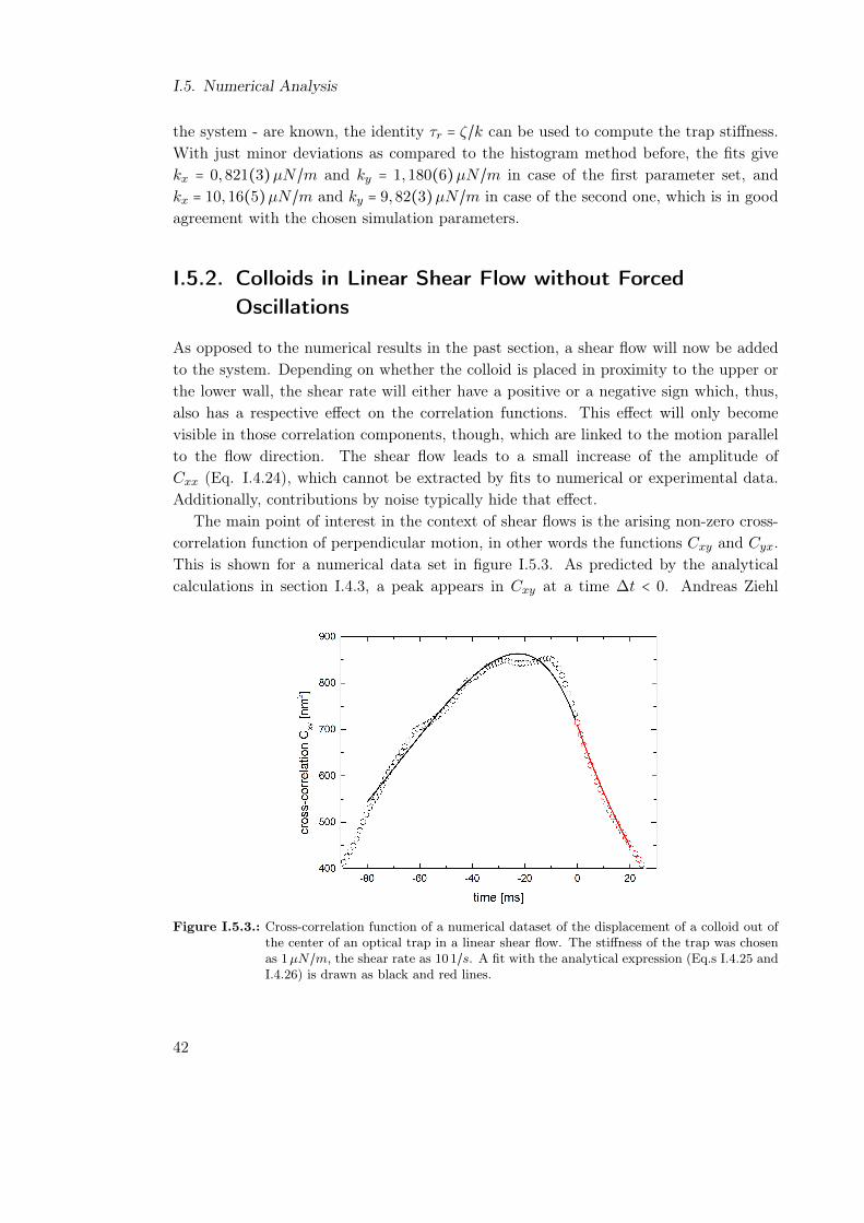
I.5. Numerical Analysis
the system - are known, the identity τr = ζ/k can be used to compute the trap stiffness.With just minor deviations as compared to the histogram method before, the fits givekx = 0,821(3)µN/m and ky = 1,180(6)µN/m in case of the first parameter set, andkx = 10,16(5)µN/m and ky = 9,82(3)µN/m in case of the second one, which is in goodagreement with the chosen simulation parameters.
I.5.2. Colloids in Linear Shear Flow without ForcedOscillations
As opposed to the numerical results in the past section, a shear flow will now be addedto the system. Depending on whether the colloid is placed in proximity to the upper orthe lower wall, the shear rate will either have a positive or a negative sign which, thus,also has a respective effect on the correlation functions. This effect will only becomevisible in those correlation components, though, which are linked to the motion parallelto the flow direction. The shear flow leads to a small increase of the amplitude ofCxx (Eq. I.4.24), which cannot be extracted by fits to numerical or experimental data.Additionally, contributions by noise typically hide that effect.
The main point of interest in the context of shear flows is the arising non-zero cross-correlation function of perpendicular motion, in other words the functions Cxy and Cyx.This is shown for a numerical data set in figure I.5.3. As predicted by the analyticalcalculations in section I.4.3, a peak appears in Cxy at a time ∆t < 0. Andreas Ziehl
Figure I.5.3.: Cross-correlation function of a numerical dataset of the displacement of a colloid out ofthe center of an optical trap in a linear shear flow. The stiffness of the trap was chosenas 1µN/m, the shear rate as 10 1/s. A fit with the analytical expression (Eq.s I.4.25 andI.4.26) is drawn as black and red lines.
42

I.5.3. Colloids in Linear Shear Flow Forced by an Oscillating Optical Trap
reported this effect in 2009 [5], however in his case the peak could be found at positivetimes while otherwise showing the exact same properties. This is due to the fact thatthe general definition of cross-correlation functions he used reads Cxy,Ziehl = ⟨x(t)y(0)⟩,while in the scope of this thesis both functions are switched by definition (Eq. I.4.18).According to the symmetry properties of correlation functions, this is identical to a time-reversal (Eq. I.4.19). Thus, the results found here can be considered in agreement withthe results of Ziehl et al.
If for the example in figure I.5.3 the fitted correlation amplitude is compared to theanalytical predictions (Eq.s I.4.25 and I.4.26), one finds a fitted value of 729(7)nm2
as opposed to an analytical one of 762nm2. Within the limits of numerical errors andstatistical noise due to the Brownian processes, such deviations are to be expected. Errorsfrom the fitting procedure have to be taken into account as well. The relaxation ratefrom the fit of 4.5(3)ms matches the analytical prediction of 3.8ms well, too.
I.5.3. Colloids in Linear Shear Flow Forced by an OscillatingOptical Trap
In this section, the full expressions for the influence of an oscillating optical trap derivedin section I.4.4 shall be probed in terms of their validity. The main focus will be cen-tered around the oscillatory contributions since, according to the analytical calculations,the terms from the stochastic integrals remain unchanged. Said oscillatory contribu-tions depend on the driving amplitude B, the driving frequency ω or respectively thedimensionless frequency α, and also the applied shear rate γ or respectively the Weissen-berg number Wi (Eq.s I.4.31, I.4.32, I.4.36, and I.4.37). A series of simulation runs wasperformed to check the dependence of the numerical results on these parameters.
As an exemplary result, the correlation functions of one of the simulation runs aredisplayed in figure I.5.4. As mentioned before, each of the auto- and cross-correlationfunctions contains oscillatory contributions (Fig. I.5.4a). This is due to the shear cou-pling. Still, the previously discussed exponential relaxation processes (Sect.s I.4.3 andI.5.2) are present and can be detected in close proximity to ∆t = 0 (Fig. I.5.4b). Thesame is true for the cross-correlation function, however, the asymmetric correlation peakis so small as compared to the oscillations, that it becomes a difficult task to identify it.By subtracting the oscillatory contributions, it can be made visible again as shown infigure I.5.4c. An additional property of shear flows in rectangular channels is that a beadplaced close to the channel walls will experience a non-zero flow velocity which leads toa shift of its equilibrium position away from the center of the optical trap. This becomesapparent in figure I.5.4c as well, since the correlation peak does not relax back to zerobut towards a smaller value. One must also take into account that, due to the influenceof Brownian noise, the oscillations can never be eliminated completely by the subtraction
43
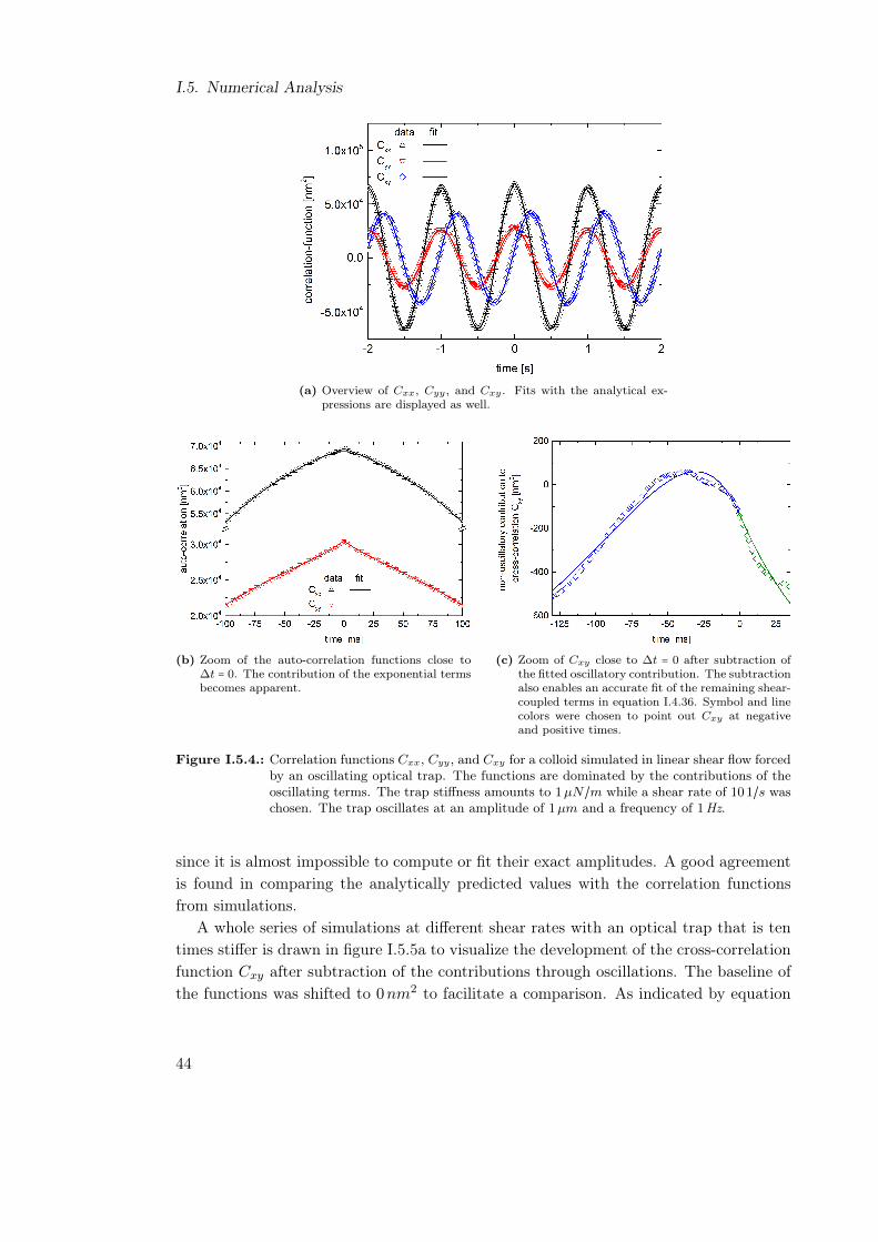
I.5. Numerical Analysis
(a) Overview of Cxx, Cyy , and Cxy . Fits with the analytical ex-pressions are displayed as well.
(b) Zoom of the auto-correlation functions close to∆t = 0. The contribution of the exponential termsbecomes apparent.
(c) Zoom of Cxy close to ∆t = 0 after subtraction ofthe fitted oscillatory contribution. The subtractionalso enables an accurate fit of the remaining shear-coupled terms in equation I.4.36. Symbol and linecolors were chosen to point out Cxy at negativeand positive times.
Figure I.5.4.: Correlation functions Cxx, Cyy, and Cxy for a colloid simulated in linear shear flow forcedby an oscillating optical trap. The functions are dominated by the contributions of theoscillating terms. The trap stiffness amounts to 1µN/m while a shear rate of 10 1/s waschosen. The trap oscillates at an amplitude of 1µm and a frequency of 1Hz.
since it is almost impossible to compute or fit their exact amplitudes. A good agreementis found in comparing the analytically predicted values with the correlation functionsfrom simulations.
A whole series of simulations at different shear rates with an optical trap that is tentimes stiffer is drawn in figure I.5.5a to visualize the development of the cross-correlationfunction Cxy after subtraction of the contributions through oscillations. The baseline ofthe functions was shifted to 0nm2 to facilitate a comparison. As indicated by equation
44

I.5.3. Colloids in Linear Shear Flow Forced by an Oscillating Optical Trap
(a) Zoom of Cxy close to ∆t = 0 after the removalof the oscillatory contribution. A continuous in-crease of the height of the peak with increasingshear rate becomes apparent, scaling linearly withthe Weissenberg number.
(b) Dependence of the oscillation amplitudes of theauto- and cross-correlation functions on the shearrate. The results from fits show that Cxx,osc ∝
γ2.03(1), Cyy,osc ∝ −0.02(1)γ, and Cxy,osc ∝
0.99(1)γ.
Figure I.5.5.: Dependence of the height of the correlation peak in Cxy and of the oscillation amplitudesof the correlation functions on the shear rate. Simulation runs for shear rates between1 1/s and 100 1/s were performed while all other parameters remained unmodified (B =
1µm, f = 1Hz, k = 10µN/m). The corresponding data sets can be found in table D.1.
I.4.36, the correlation peak increases in height linearly with the shear rate or respectivelythe Weissenberg number, while its width does not change. This effect is clearly visibleat shear rates higher than 50 1/s, while at lower values the peak nearly disappears inthe background noise. Assuming that a similar effect might appear when evaluatingexperimental results, it hints towards high shear rates, i. e. γ ≥ 20 1/s, being necessary ata trap stiffness of 10µN/m. The quality of the peaks at low shear rates can be improvedby choosing an increased number of simulated data points or in other words a longermeasurement length (i. e. 64 s) at the same recording frequency. In this context, theconvergence of the algorithm was checked as well by an increased measurement lengthand an increased recording frequency. In both cases, the algorithm produced stableresults with a comparable functional form and height of the peaks in Cxy.
When looking at the oscillatory amplitudes of the auto- and cross-correlation functionsinstead (Eq.s I.4.31, I.4.32, and I.4.36), one would assume that Cyy,osc is independent ofthe shear rate, Cxx,osc is proportional to its squared value, and Cxy,osc increases linearlywith it. Fits to the oscillatory contributions to correlation functions from the same datasets as above give parameter values as displayed in figure I.5.5b (compare also Tab. D.1),and prove that the expected behavior occurs indeed.
As mentioned in the introduction to this section, not only the shear rate but also thefrequency as well as the amplitude of the driving oscillation shall be varied. A changein frequency will automatically cause a change of α, which will have its repercussions on
45

I.5. Numerical Analysis
Figure I.5.6.: Dependence of the relative correlation amplitude Cxx,osc/Cyy,osc on the oscillation fre-quency of the optical trap. A parameter set B = 1µm, k = 10µN/m, and γ = 10 1/swas chosen for all simulations. A fit of the values up to 60 rad/s to a power lawgives Cxx,osc/Cyy,osc ∝ ω2.00(1), for frequencies higher than 300 rad/s the fit givesCxx,osc/Cyy,osc ∝ ω3.53(8). The crossover of both fits happens at about 185 rad/s. Thecorresponding data sets are provided in table D.2 in the appendix.
all of the correlation functions. These changes encompass not only the amplitude of theoscillatory terms Cij,osc, but also the phase behavior of Cxy. To visualize this, a seriesof simulations under variation of the driving frequency were performed. With regard tolater experiments, it must be remarked that the trap stiffness for frequencies higher than60 rad/s is simply not high enough to successfully confine a particle in the experimentalsetup in a shear flow with γ ≥ 10 1/s. In that case, the stiffness needs to be furtherincreased, which will lead to a disappearing of all special features of the correlation func-tions, since their amplitudes decrease under these conditions. Experimentally speaking,only a frequency range up to ≈ 60 rad/s is accessible in this respect.
The dependence of the correlation amplitudes on the driving frequency is presented inthe form of the auto-correlation amplitude ratio Cxx,osc/Cyy,osc (Fig. I.5.6). Accordingto equation I.4.38, for small frequencies ω ≪ 1/τr, or in other words α≪ 1, the amplituderatio decreases proportionally to ω−2, while for the opposite case ω ≫ 1/τr it will decreaseproportionally to ω−4. If the results from simulations are compared to this prediction, thebehavior for small frequencies (up to 60 rad/s) is recovered with a very high precision(Cxx,osc/Cyy,osc ∝ ω−2.00(1)), while at higher frequencies (above 300 rad/s), there aredeviations from the predicted power law (Cxx,osc/Cyy,osc ∝ ω−3.53(8)). The change inpower occurs at about 185 rad/s, which is given by the cross-over frequency of the redand blue curve corresponding to the low and high frequency power law fits (Fig. I.5.6).
46

I.5.3. Colloids in Linear Shear Flow Forced by an Oscillating Optical Trap
The critical transition frequency can also be computed by
ωcrit =1
τr= 265
rad
s. (I.5.5)
The deviation between the analytic value and the value from the crossover is due to theimprecision when graphically determining the frequency value in the log-log-plot. Thevalue in equation I.5.5 can be considered as exact. The relaxation rate τr needs to bedetermined by the quotient of the coefficient of friction and the trap stiffness present inthe system. In the experimental context, the assumption of moving in the low-frequencyrange is justified, which enables the application of a simplified calculation of the shearrate following from equation I.4.38
limα≪1
Cxx,osc
Cyy,osc≈ γ
2
ω2. (I.5.6)
A further reflection will concern the development of the phase of the oscillatory termin Cxy in respect to the driving frequency. For the remainder of this part, only the phaseof Cxy will be discussed since the oscillatory part of Cyx is just given as the time-reversedfunction and thus, the relationship of both phases can be expressed as (compare Eq.sI.4.36 and I.4.37)
δ(Cxy,osc) = −δ(Cyx,osc) = −arctan( 1
α) . (I.5.7)
The phase behavior is exclusively determined by the dimensionless frequency, composedof the product of the driving frequency ω with the relaxation rate τr. Since for alllater experiments, water is always chosen as the fluid in which the colloids are immersedand since the colloid size was always the same at 4µm, the relaxation rate is solelydetermined by the strength of the optical trap. The phase is completely uninfluencedby flow parameters like the shear rate. Figure I.5.7 shows that the phase behavior fromnumerical simulations agrees indeed with theoretical predictions as displayed earlier infigure I.4.11. For the relaxation rate determined by fits, the analytical curve can becalculated. It is also displayed in figure I.5.7 as a red line. Analytical predictions andfitting results from numerical data agree to a very high degree.
47

I.5. Numerical Analysis
Figure I.5.7.: Phase behavior of Cxy as a function of the dimensionless frequency. The relaxation rateτr remains fixed by choosing a constant trap stiffness 10µN/m for all simulation runs.The corresponding data sets are displayed in table D.2 in the appendix.
48

I.5.4. Summary
I.5.4. Summary
In this chapter, the system of a colloid confined in the focal region of an optical trapwas exposed to a variety of flow situations in numerical simulations. For this purpose,the analytical framework developed in chapter I.4 was recast into a form suitable for aniterative numerical algorithm (Eq.s I.5.2 and I.5.3). In section I.5.1, as a trial run, a qui-escent flow situation was assumed, meaning that there existed no shear flow and also nodriving force was applied. Out of this, symmetrical Gaussian-like position distributionsresulted. These could be used as a means to calibrate the strength of the optical trap orin other words the trap stiffness k. An almost symmetric trap could be recovered by thisprocedure, where deviations from the ideal case were caused by the noise-like nature ofBrownian motion. From the same data sets, the equilibrium auto- and cross-correlationfunctions could be determined (Fig. I.5.2). A further check was performed in sectionI.5.2 by applying a shear flow to the bead and comparing the arising situation with theequilibrium case from before. While there was no directly apparent change as far as theauto-correlation functions Cxx and Cyy are concerned, there was a very clear alterationof the cross-correlation function (Fig. I.5.3). As already found by A. Ziehl [5] and J.Bammert [18], a correlation peak appears in Cxy close to, but not exactly centered at,time zero. It is caused by the short delay the fluctuating bead needs to adapt to thefaster or slower flow slightly above or below the position of the optical trap in y-directionin the assumed shear flow. The algorithm seems well-suited for the task of simulatingcolloids in shear flows.
In section I.5.3, a forced oscillatory motion of the center of the optical trap was addedto the system as already done before during the analytical calculations in section I.4.4.All the properties of the sheared case without forced oscillations were still present, how-ever, each correlation function showed an additive oscillatory term just as predicted bythe analytical framework. By analyzing the dependence of the oscillatory correlationamplitudes Cxx,osc, Cyy,osc, and Cxy,osc on the shear rate as well as the amplitude ra-tio Cxx,osc/Cyy,osc and the phase behavior δ(Cxy,osc) on the driving frequency, a goodagreement with the analytical predictions could be found.
The analytical expressions found in chapter I.4 and the numerical simulations dis-cussed in this chapter will be of help in understanding and interpreting the experimentsconducted in a setup of optical tweezers (Ch. I.6). Not only a qualitative, but also aquantitative agreement between the three will be checked in order to confirm certainparameters system-internal like the local shear rate.
49


I.6. Experimental Study
The current chapter is related to all the information linked to the conduction of expe-riments with the setup of optical tweezers present in the Wagner group in the physicaldepartment of Saarland University in Saarbrücken, Germany. Before the performed expe-riments will be discussed, in the first section of this chapter (Sect. I.6.1) the compositionof the setup is described. This includes an in-depth discussion of the changes the setupunderwent since its construction by Andreas Ziehl [4, 5]. In the second section (Sect.I.6.3), a number of steps necessary for the calibration of the experimental setup are de-tailed. A description of the types of measurements conducted in the scope of this partof the thesis, as well as their results are presented in section I.6.4. Their discussion incontext with analytical and numerical results from earlier chapters (Ch.s I.4 and I.5) willfollow in chapter I.7.
I.6.1. Experimental Setup
The setup of optical tweezers that was utilized in this thesis to perform experiments withcolloids in a linear shear flow (pt. I) as well as microrheology on mucus (pt. II) will bedescribed in this section.
It can be roughly divided into three constituents: the guidance system of the laserbeam(s), the microscope including the visualization technology, and the flow control forthe microchannels. While the flow control only plays a role in the first part and not formicrorheology, the other two components of the setup are important for any experimentperformed in it. Respectively, this section will be divided into three subsections givingdetails about each of these parts, and also pointing out differences as compared to thesetup used before by Andreas Ziehl.
51

I.6. Experimental Study
I.6.1.1. Guidance System of the Laser Beams
Hereinafter, the beam path of both available laser beams in the setup will be describedstarting at the laser sources until the beams arrive in the sample cell of the microscope.This path is also indicated in figure I.6.1 in the shape of a photograph as well as a sketch.
As already mentioned in chapter I.3, the central element of such a setup is a stronglyfocused laser beam. The force balance of the scattering and the gradient force exertedon a small object, i. e. a colloid, determines if a stable optical trap can be formed ornot. Since the gradient force gains the most strength relative to the scattering force ifthe laser beam has the smallest intensity at its center while having a high intensity nearits outer radius, a transverse electromagnetic TEM01∗ mode beam would be ideal. Itsprofile reminds of the cross-section of a doughnut - hence its name doughnut mode - butit also comes with a share of disadvantages. The biggest of these is the construction ofthe laser necessary to emit it. This is the reason why in most setups of optical tweezersGaussian-shaped beams of the TEM00 mode are used. On the first glance, their beamprofile is disadvantageous for efficient trapping since the maximum intensity can be foundin the center of the beam. By overfilling the back aperture of the microscope objective inthe setup [63], the outer rays of the beam gain more intensity in comparison to the centerbeams which makes strong traps possible without increasing price and complexity of thesetup. Thus, in case of the setup used in scope of this thesis, two lasers are available,both of which are diode-pumped solid-state lasers. The first one operates at 532nm
(Ventus LP, Laser Quantum Ltd., Stockport, Cheshire, United Kingdom), the second oneat 473nm (Ciel, Laser Quantum Ltd., Stockport, Cheshire, United Kingdom). In bothcases, the emitted spatial mode is a transversal electromagnetic mode of the TEM00 type,which shows a two-dimensional Gaussian intensity distribution in the plane perpendicularto the propagation direction of the beam. Both lasers produce beams of high stability ofless than 2 % rms for the Ventus model and, respectively, less than 3 % rms for the Cielmodel. The beam divergences are small with values of 0.8mrad and 0.6mrad. Theseproperties ensure the generation of stable optical traps of high homogeneity. However,since the diameters of both beams are not equal (Ventus: db = 1mm, Ciel: db = 1.4mm),beam expanders with different expansion factors have to be used to ensure equally sizedtraps. Additionally, they take care of the required overfilling of the back aperture of themicroscope objective.
Since the knowledge of the laser power is important when determining the strengthof an optical trap, the stability of the emission and also the dependence of the emittedpower on the applied current was measured using a power-meter (Fig. I.6.2). Within theprecision limits of the sensor, which were given by the manufacturer as ±100µW , none ofthe lasers showed significant fluctuations. As the figure shows, the power against currentdependence is not a linear one, making a calibration of the trap stiffnesses necessarybefore each experiment. Details about the calibration options and procedures are given
52

I.6.1. Experimental Setup
(a) Photograph of the setup of optical tweezers as seen from above.
(b) Schematic sketch of the full beam path of the lasers as well as theillumination source.
Figure I.6.1.: Illustration of the setup of optical tweezers.
53

I.6. Experimental Study
Figure I.6.2.: Power of each of the laser beams measured by a power meter. The sensor was placedin the beam path just behind the source. The corresponding data sets are presented intables D.3 and D.4 in the appendix. Due to thermal noise in the surroundings of thesensor, the data has a precision of ±100µW .
later in this chapter (Sect. I.6.3). Additionally, as a means to check the quality of thebeam profiles, they were visualized on the chip of a CCD camera after a reduction oftheir intensities using both an OD2 and an OD4 filter1.
Due to the different beam diameters, as mentioned, two beam expanders with corre-sponding optical properties had to be set up in the beam paths. As indicated in figureI.6.1, they were placed about 10 cm behind the aperture of the laser. For the 532nm beama 10x-expander (art.-no. G038-670-000, Linos Photonics GmbH & Co. KG, Göttingen,Germany) was used, while for the 473nm beam a 8x-expander (art.-no. G038-678-000,Linos Photonics GmbH & Co. KG, Göttingen, Germany) was chosen.
Although this possibility was not used in the experiments presented here, the setup isdesigned in a way that allows both optical traps to be used simultaneously. This leads tothe necessity of superimposing both beams into one. For this purpose, the 532nm beamis first redirected by an angle of 90○ using a piezoelectric mirror and then combined withthe 473nm beam using a dichroic mirror. The piezoelectric mirror can be pitched andyawed by two ultra-high resolution rotational actuators (PZA12, Newport Corporation,Irvine, CA, United States of America), which when combined with a mirror mount (U200-G, Newport Corporation, Irvine, CA, United States of America) allow angular steps inthe order of magnitude of µ-radians (sensitivity according to manufacturer: 30nm). Thisenables a very exact control of the relative trap positioning. The dichroic mirror on the
1“OD” is an abbreviation for optical density and gives an indication of the intensity reduction expressedon a logarithmic scale. An optical density of 2 represents an intensity reduction by a factor of 102, anoptical density of 4 represents a reduction by a factor of 104.
54

I.6.1. Experimental Setup
(a) Beam profile of the laser operating at 532nm. (b) Beam profile of the laser operating at 473nm.
Figure I.6.3.: Beam profiles of the two lasers utilized in the setup of optical tweezers. The slightasymmetry of both profiles originates from the surface normal of the camera chip beingtilted against the propagation direction of the beams. The intensities are expressedrelative to the highest occurring intensity in each profile.
other hand is chosen in such a way, that a near-perfect reflection of the 473nm beam ispossible while the 532nm beam transmits to a high degree (≈ 94 %). The characteristicline of this filter (505DCXR, AHF analysentechnik AG, Tübingen, Germany) is drawnin figure I.6.4 with black circle symbols.
In the earlier realization of the setup as built by Andreas Ziehl, the lasers passed abeam lift at this point in order to allow for a coupling of the combined beam into theback port of the microscope. In addition, a telescope is added to the beam path. Itsfirst lens is positioned in front of the beam lift, the second one is placed behind it. Bothlenses share identical optical properties (LA1832-A, Thorlabs GmbH, Dachau/Munich,Germany) and are covered with an anti-reflection coating to prevent power loss of thelaser beams. The setup is augmented with the telescope in order to decrease divergenceeffects of the beams and to fine-tune the positioning of the focal plane of the lasers afterpassing the microscope objective or, in other words, the distance of the optical trapsthemselves.
At this point, the laser beams enter the back port of the inverted microscope (EclipseTE2000-S, Nikon GmbH, Düsseldorf, Germany). Besides the lasers, this microscope isthe second central device of the setup. Here, an inverted microscope is chosen since itallows the manipulation of confined objects in the traps while at the same time enablingtheir visualization using light directed inversely to the lasers. More information about itwill follow in the next section. However, a few more elements involving the guidance ofthe laser beams have not been mentioned so far and shall be discussed first. After enteringthe microscope, the beams have to be redirected upwards in order to enter the objectivefrom below and finally reach the sample cell. A second dichroic filter (565DCXR, AHFanalysentechnik AG, Tübingen, Germany) is installed inside a filter block to fulfill that
55

I.6. Experimental Study
Figure I.6.4.: Characteristic transmission line for both of the dichroic mirrors utilized in the setup ofoptical tweezers. In addition to the filter lines, the two characteristic wavelengths of theutilized lasers are drawn as accordingly colored lines at 532nm and 473nm. The datasets were provided by courtesy of the manufacturer AHF analysentechnik AG.
role. Its properties are chosen in such a way, that contrary to the properties of thedichroite mentioned before, both laser wavelengths are reflected to a high degree (> 99 %,compare the red open circles in Fig. I.6.4). This filter enables the beams to reach thesample cell after passing the objective while, at the same time, allowing the illuminationlight to reach the camera.
I.6.1.2. Microscope, Visualization, & Signal-Synchronization System
In this section, the focus will be laid on the microscope and its directly related systems.As already mentioned before, an inverted microscope by Nikon is chosen for the setup ofoptical tweezers in Saarbrücken (Eclipse TE2000-S, Nikon GmbH, Düsseldorf, Germany).Especially in context with such a setup, inverted microscopes have huge advantages.They allow to send laser beams associated with optical tweezers into a sample cell andthus to confine and manipulate colloids. At the same time, the traps are not fixedand can be moved within the sample, giving a high degree of mobility. This is realizedby realigning the positions of the optical traps, however, a much easier method is therelative displacement through a mechanical translation of the microscope stage. Sincethe visualization of the displacements of colloids is of crucial importance in this thesis,this is a necessary prerequisite to the setup as well. Due to its alignment, it is possibleto orient the beam path of illumination light in reverse to the laser beam path, and thusrecord the motion of colloids with a suitable recording device. Details will be mentionedlater in this section.
Vibrations, particularly the avoidance of external vibrations, play a very important
56

I.6.1. Experimental Setup
role in any setup of optical tweezers. Since these setups aim at recording Brownian mo-tion, which is a noise-based process, any additional external noise makes the interpreta-tion of measurement hard or even close to impossible. Thus, a vibration dampening tableby Halcyonics named Active Workstation 1100 (Halcyonics GmbH, Göttingen, Germany)is used. Only those devices and elements which are needed close by for the conductionof experiments are placed on top of that table. All elements that cause additional vibra-tions like the illumination source, which is actively cooled by a fan, are removed from thetable and situated below or next to the table on stands instead. Also, a laboratory inthe cellar of the building is chosen to prevent strong influences by low-frequency buildingvibrations, which cannot be efficiently removed by the dampening table.
As noted above, displacements of the field of view and, linked to that, of the positionsof the traps can be performed by mechanically moving the microscope stage. However,the resolution of such displacements is limited. An improvement can be administered bymounting a piezoelectric stage on top of the mechanical one. For this purpose, a stageby PI is chosen (P-517.2CD, Physik Instrumente (PI) GmbH & Co. KG, Karlsruhe, Ger-many) in combination with two controllers (E-665.CR, Physik Instrumente (PI) GmbH& Co. KG, Karlsruhe, Germany), one for each translation direction. With a travel pathof up to 200µm at a spatial resolution of 2nm, a very precise positioning of the trapscan be achieved. Since in this part of the dissertation, oscillatory motion will play animportant role, the linearity error of 0.03 % and the repeat accuracy of ±10nm are note-worthy as well. According to the voltage calibration of the manufacturer, displacements∆xi are linked to applied input voltages U by
∆xi ≈ 10.0012µm
V⋅U , (I.6.1)
where i represents the respective direction of the displacement, i. e. x or y. The voltageamplification of the controller of 10x is already taken into account with this calibration.The controllers also enable the coupling of an external electric signal into the stage.The signals necessary to steer the piezoelectric stages are typically created by a signalgenerator. Here, a device by Thurlby Thandar (TG230, Thurlby Thandar InstrumentsLimited, Huntingdon, Cambridgeshire, United Kingdom) is used which allows outputamplitudes of sinewaves between 20mV and 20V and frequencies between 2mHz and2MHz.
Some additional optical elements and filters are involved in the construction of themicroscope. One of them is the objective, which is an oil-immersion objective with a 60xmagnification and a numerical aperture of NA = 1.4 (mat.-no. MRD01602, Nikon GmbH,Düsseldorf, Germany). As already discussed in context with the scattering regimes inoptical tweezers (Ch. I.3), a high numerical aperture is crucial for an efficient trappingsince it increases the gradient force as compared to the scattering force and hence sta-bilizes the optical trap. The objective utilized in this study is designed for the use with
57

I.6. Experimental Study
Figure I.6.5.: Characteristic transmission line for the two rejection band filters utilized in the setup ofoptical tweezers. Additionally to the filter lines, the two characteristic wavelengths ofthe utilized lasers are drawn as accordingly colored lines at 532nm and 473nm. Thedata sets were provided by courtesy of the manufacturer AHF analysentechnik AG.
coverslips and has a focal length of 170µm.Below the filter block which carries the dichroic filter for redirecting the laser beams
through the objective, an additional filter is placed. It prevents any misguided laser radi-ation to reach the eyes of the user or the chip of the high-speed camera (art.-no. F62-456,AHF analysentechnik AG, Tübingen, Germany). A second filter of this type is insertedinto the ocular of the microscope to shelter the eyes even more. At the wavelengths ofthe utilized lasers, each of the filters offers an optical density of more than 6 as indicatedby the characteristic line in figure I.6.5. While blocking the laser radiation, however,the radiation of the illumination source still needs to pass these filters since otherwisea visualization of the surroundings of the optical traps would be impossible. Thus, thistype of filter is ideally suited for this purpose.
This section is also intended for the description of the visualization system of thesetup. It consists mainly of an illumination source, a condenser, the microscope objectivedescribed earlier in this section, and a high-speed camera. The dichroic filter 565DCXRand the aforementioned rejection band filters are also part of it, but since they havealready been discussed, they will be omitted here. The illumination source used in thesetup in Saarbrücken is LED-based (light emitting diode) and consists of a single high-power white-light LED source. Since there is no diode that emits at multiple wavelengthsat the same time, such LEDs are realized by mixing the contributions of different opticaltransitions of multiple semi-conducting materials2. This is also the case for the model
2Typically, for this purpose a galliumnitride (GaN) or a indiumgalliumnitride (InGaN) transition com-
58

I.6.1. Experimental Setup
used here, which is a Zett ZLED 9000 CLS by Zett Optics (art.-no. 799000, OptoSysGmbH, Darmstadt, Germany). Since the light source has its own casing, it is set up belowthe laboratory bench and only an optical fiber needs to be mounted to the microscope.This contributes to reduce the amount of mechanical noise in the setup. The modelEclipse TE2000-S offers an extension arm above the condenser, which is designed speciallyfor the purpose of aligning light sources. Before the integration of this light source,Andreas Ziehl utilized a halogen lamp by Schott. However, in combination with thehigh-speed camera model currently used in the setup at typical recording frequenciesof 8 kHz, strong intensity fluctuations due to the AC power supply of the lamp becomeapparent and reduce the quality of the recorded pictures. This effect also reduces theprecision of particle tracking which will be explained later (Sect. I.6.2). Replacing thelamp with an equally or even more powerful lamp on a non-alternating current basis ispreferable. The Zett ZLED 9000 CLS has exactly these properties and shows almost nofluctuations, although still being supplied by an AC current. Supporting lenses, mountedto the microscope arm, optimize the beam divergence further to couple as much light aspossible through the sample cell and into the camera.
Before reaching the sample cell, the light from the illumination source reaches a con-denser (TI-C-CLWD 0.72, Nikon GmbH, Düsseldorf, Germany) with a numerical apertureof NA = 0.72 which focuses the light into the cell. After passing through it, the lightcrosses the objective as well as the dichroic and the rejection band filter and propagatestowards either the ocular or the camera, depending on the setting of the microscope. Asa camera, the model HighSpec 1 by the manufacturer Fastec Imaging3 (Fastec Imaging,San Diego, CA, United States of America) is used. It offers a camera chip with 1,280pixels in width and 1,024 pixels in height at an 8-bit greyscale resolution. The pixelsize is 14µm × 14µm and it enables a temporal resolution of 506 pictures per second atfull-frame resolution while allowing recording rates up to 20 kHz at a reduced resolutionof 128px × 64px. When taking the 60x magnification of the objective into account, thisgives a pixel size of 233.3nm×233.3nm. The camera also offers 2GB of internal memory,making the recording of about 250,000 pictures at reduced resolution within about 16 s
possible.In order to record oscillatory forced motion of colloids, it is necessary to couple these
oscillations into the system and at the same time synchronously record the confined col-loids. The synchronization is realized by a custom-built trigger box. It was manufacturedby the electronics workshop of the experimental physics department in Saarbrücken. Itreceives a 5V TTL-pulse as input and down-converts it to a 3.3V low-voltage TTL-pulse,but only if a mechanical, debounced switch is activated. Now, this TTL-signal is usedto start the recording of the camera while at the same time the electrical driving signal
bined with a cerbium: yttrium-aluminium-garnet (Ce:YAG) transition is used.3The model is identical to the camera MotionBLITZ EoSens mini1 by Mikrotron, Unterschleißheim,Germany.
59

I.6. Experimental Study
stemming from the same frequency generator as the TTL-signal is sent to the piezoelec-tric stage. If both the TTL-signal and the driving signal are recorded, the pictures takenby the camera and the motion of the stage can be synchronized. The data acquisitionof these signals is performed by a National Instruments analog input module (NI 9215,National Instruments, Austin, TX, United States of America) which is then recorded by acustom program written in the graphical programming environment LabVIEW (versions2010 to 2013, National Instruments, Austin, TX, United States of America).
I.6.1.3. Flow Control in the Microfluidic Device
In the scope of this thesis, flows through small channels of microfluidic devices are used tocreate shearing close to their walls. There exists a variety of ways to produce such flows,the most popular among which are probably syringe pumps. In these devices, a syringeis fixed inside a mechanism which is set to empty or fill the syringe at a constant flowvelocity. Other velocity profiles can typically be chosen or programmed as well. However,these systems only offer a limited accuracy when choosing slow emptying velocities andare also sensitive to irregularities in the manufacturing of the syringes. This leads tonon-constant flow velocities and thus ill-defined shear gradients which vary over time.Thus, in the setup instead of syringe pumps a passive systems was utilized that uses thehydrostatic pressure difference of an inlet reservoir positioned at a greater height thanthe outlet reservoir. The pressure difference in the system is caused exclusively by theweight of the fluid column between inlet and outlet
∆p = ρg∆h , (I.6.2)
where ρ is the fluid density, g the gravitational acceleration, and ∆h the height differencebetween in- and outlet. The flow velocity can thus be tuned by slightly changing theheight difference by moving the inlet reservoir up or down. Theoretically, the flow velocitywill decrease over time since the reservoir is not infinitely large. On the one hand,it takes a very long time until the reservoir is emptied completely which means thatover the course of a single measurement, no variations in flow velocity need to be takeninto account. After each experiment, the height can be re-adapted to reach the desiredvelocity. Thus, the flow velocity is assumed to remain stable.
Such a system is realized in the setup of optical tweezers in Saarbrücken. As reservoirs,syringe bodies with their pistons removed (art.-no. 4606027V, B. Braun MelsungenAG, Melsungen, Germany), equipped with needles of a diameter of 0.6mm (art.-no.4657667, B. Braun Melsungen AG, Melsungen, Germany) are chosen. The syringe offersan experimentation volume of more than 2ml. Leakage can be avoided since the sizeof the needle tightly fits into the tubing connected to the microfluidic device. Theproduction of the microfluidic device has already been described earlier (Sect.s I.4.2 andA.2.1). As in- and outlet tubing, polyethylene oxide (PEO) tubes with an inner diameter
60

I.6.2. Utilized Software
of 0.5mm and an outer diameter of 1mm are used (art.-no. 3550501, Laborshop24,Gross-Zimmern, Germany).
For such a kind of gravitational driving of flows, a reproducible way of setting theheight of the reservoirs is necessary. In the utilized setup, two linear motors of type LTM80F-300-HiDS (art.-no. 41.084.30GJ, Owis, Staufen, Germany) with one controller oftype PS10-32-DC each (art.-no. 55.11.2432, Owis, Staufen, Germany) are used. Theyare mounted perpendicular to the surface of the laboratory bench. The mounting aidsare about 1m long aluminium boards with threaded holes for fixing the motor to it.The boards were custom-built by the mechanical workshop of the experimental physicsdepartment in Saarbrücken. The same is true for the fixtures that were used to attachthe syringe bodies to the moving slide of the device. By moving the motors back andforth, the height of the reservoir can thus be set with very high precision. Both motorsoffer a long travel path of 21 cm at a low positioning error of less than 25µm/100mm anda bidirectional repeatability within ±15µm. The motors can be attached to a computerwhich allows the steering of the devices. As an additional driving option for the flows,a compressed air bottle can be attached to the tops of the open syringe bodies viatubing. Since such a bottle provides a pressure of 2 ⋅107 Pa, it needs to be adapted usingpressure reducing regulators (pmax = 7,000Pa). This is particularly useful when colloidsor dust particles block the microchannels, since the higher pressure tends to unblock thechannels and pumping the contamination out of them. They should be avoided in thefirst place, but even under cleanroom conditions this is not always possible; blockagethrough sedimentation of particles within the channels is taking place during the wholecourse of the experiments, independent of how clean and dust-free the channels are.
I.6.2. Utilized Software
There is a number of software applications that are used in this work to acquire datasetsduring the course of experiments and also to process and evaluate them later. Some ofthese are written in LabVIEW (versions 2010 to 2013, National Instruments, Austin,TX, United States of America), others are realized in Matlab (version R2011b, TheMathWorks, Inc., Aachen, Germany). In this section, a listing of these applications withinformation about the environment they were developed in will be given. In some ofthese cases, more details will be added about the algorithms.
When performing experiments in a setup of optical tweezers, the motion of a single ormultiple confined colloids needs to be recorded and, at a later stage, tracked, so a list ofparticle positions is created which allows further processing. In the setup in Saarbrücken,a high-speed camera by Fastec Imaging is used (see also Sect. I.6.1.2) which offers aproprietary software for recording images. A variety of image formats is offered as well.When operating the camera in high-speed mode, a huge number of pictures is createdin a short amount of time. Since the operating system Microsoft Windows XP does not
61

I.6. Experimental Study
handle huge numbers of files with a particularly good performance, a picture containerwith file extension “.raw” is chosen. The images are saved within this file as a string ofheader-less “.tif” files. They can be transferred from the internal memory of the camerato the hard disk drive of the computer within about 3 minutes, assuming that the internalmemory has been filled entirely.
During the course of the experiments, sometimes, an online realignment of the po-sition of the optical traps is necessary. In general, this requires the realignment of thewhole setup. However, if only the trap generated by the 532nm laser beam needs to berepositioned, this can also be achieved by carefully moving it through manipulation of theorientation of the piezoelectric mirror in the beam path. It can either be controlled by us-ing electrical switches or by a software written by Andreas Ziehl in LabVIEW [4]. Whenworking with a microfluidic device and a change of the flow velocity is desirable, this ispracticable by adapting the height of the syringe body attached to a linear motor. Thesesettings can be chosen in a proprietary application called OwiSoft that was distributedalongside the motors. It allows not only to set a displacement, but also the driving ofthe motor with a certain velocity profile. However, these options are not necessary forthe conduction of the experiments, so simply setting a height is already sufficient.
As mentioned before in section I.6.1.2, in order to determine the reaction of a confinedcolloid to a shear flow, it is necessary to record the electric sinewave signal in synchronicitywith the images recorded by the camera. A custom virtual instrument in LabVIEW wasdesigned to acquire the input sinewave together with the TTL-signal triggering the startof the recording by the camera.
After the successful transfer of pictures from the camera to the hard drive, an option isneeded to extract the particle positions. This is achieved by an application developed byAchim Jung [64] in which each of the images is Fourier-transformed and then correlatedwith a template image (typically the first image of a measurement). By applying a two-dimensional Gaussian fit, the shift of the particle from the current image as comparedto the template can be determined with sub-pixel resolution. Since the characteristiccircumference of the colloid in each picture covers a multitude of pixels, the accuracyof the fitting procedure is improved immensely. As a result, the software gives a list ofx- and y-displacements and the picture number, which can be used as a time axis. Theoriginal program of A. Jung was slightly modified to directly accept the “.raw” format ofthe high-speed camera, saving the time and effort necessary for a conversion.
Since in part I of this dissertation, auto- and cross-correlation functions play a centralrole, a software is needed which is able to handle very large data sets created by eachmeasurement and to calculate these functions. It was custom-developed in LabVIEW.The specific calculation sequence is described in section C.1 of the appendix. As input,a formatted text document (“.txt” or “.dat”) with one time and two position columns inthis order is accepted, whereas the results are exported as a second text document withone time and three correlation columns Cxx, Cyy, and Cxy.
62

I.6.3. Calibration of the Setup
(a) Correlation functions for an aligned camera. (b) Correlation functions for the camera tilted by 10○.
Figure I.6.6.: Influence of the camera angle alignment on the correlation functions of the displacementsof a trapped bead. A data set from a numerical simulation was used, where an oscillationwith a frequency of 3Hz and an amplitude of 10µm was applied to the optical trap iny-direction for demonstration purposes. The trap stiffness was set to 1µN/m, no shearflow was present. The auto- and cross-correlation functions of the data set were at firstcalculated for the unmanipulated data set, then, this step was repeated after virtuallyrotating the data set by 10○.
As a general tool for handling and organizing data, Origin (version 9, OriginLabCorp., Northampton, Massachusetts, United States of America) was utilized. It allowsthe fitting of functions to data sets and also offers additional options like performing aFourier-analysis.
I.6.3. Calibration of the Setup
In this section, details about components of the setup of optical tweezers which need tobe calibrated regularly will be given. Typically, before the setup can be used, it needs tobe cleaned first using pressurized air and cleaning tissues. Afterwards, the alignment ofthe laser beam path is performed.
There are two additional elements whose alignment needs to be taken care of. Whenthe high-speed camera is attached to the side-port of the microscope, it will recordthe focal plane of the objective. However, since the camera has a rotational degreeof freedom, the tilting angle is not defined. This will play a crucial role, especiallyin context with the measurement of the correlation functions of bead displacements.To visualize the effect of a tilted camera on the correlation functions, a data set wascreated by numerical simulations where an oscillation was applied to the optical trapin y-direction while no shear flow was present. As such, due to the missing couplingeffect by the shear flow, the motion of the bead in perpendicular directions should beuncorrelated. For the unmanipulated data set, this is definitely true (Fig. I.6.6a) sinceoscillations can only be found in the auto-correlation function Cyy (not displayed due to
63

I.6. Experimental Study
Figure I.6.7.: Typical displacement curve recorded for the tilt calibration of the camera. An oscillationwas applied to the piezoelectric stage in x-direction while the camera recorded the motionof a bead that was immobilized at the surface of a coverslide. From the deviation ofthe trajectory from a horizontal line, the remaining tilting angle of the camera can bededuced. In this graph, the angle amounts to 0.107(1)○.
the large extent of the ordinate) and to a much smaller degree in the cross-correlationfunction Cxy. Cxx is still given by the pure exponential relaxation behavior from thequiescent case and shows no influence whatsoever from the oscillations. If, however,a tilt of the virtual recording device by 10○ is assumed, the situation changes (Fig.I.6.6b). The tilt is performed by transforming the data set to spherical coordinates,adding the value of 10○ to the angle, and transforming the data set back to the Cartesianframe. Now, the oscillatory contribution to the cross-correlation function is increased byroughly two orders of magnitude, while the auto-correlation function Cxx also shows anoscillatory behavior. The original exponential relaxation disappears almost completely. Itis noteworthy that these spurious correlations always occur as unshifted cosine functions,since they originate from auto-correlated contributions.
Under the assumption that such an error occurs, it is of central importance to assessthe consequences of it on the outcome of a measurement and shall be conducted as asimplified calculation. Consider a tilt of the recording device, i. e. the camera, versusthe oscillation direction by an angle β = 5○. In case of an oscillation otherwise perfectlyaligned with the y-axis, this will cause it to be mixed into the motion in x-direction. Thepercentaged change of the positions in x- and y-direction in respect to a reference positioncannot be calculated since it depends on the exact positions. Expressed in a sphericalcoordinate system, the length ∣r∣ of the position vector remains the same, while only theangle increases by β. For the sake of presentability, let us assume nonetheless that theerror can be expressed as a percentage value p. This means that motion recorded in the
64

I.6.3. Calibration of the Setup
frame of the camera C, from this moment on denoted by the Cartesian coordinates x′
and y′, can be recast to the frame of the piezoelectric stage S, expressed in the Cartesiancoordinates x and y
x′ = x ⋅ (1 − p) + y ⋅ p , (I.6.3)
y′ = x ⋅ p + y ⋅ (1 − p) . (I.6.4)
The consequence of this for the cross-correlation function can then be written as
Cx′y′(τ) = ⟨x′(t)y′(t + τ)⟩ (I.6.5)
= ⟨(x(t) ⋅ (1 − p) + y(t) ⋅ p)(x(t + τ) ⋅ p + y(t + τ) ⋅ (1 − p))⟩ (I.6.6)
= (1 − p)2Cxy(τ) + p(1 − p)(Cxx(τ) +Cyy(τ)) + p2Cyx(τ) . (I.6.7)
Hence, in the expression for the measured cross-correlation function Cx′y′ , there is notonly a contribution of Cxy, but also of all auto-correlation functions Cxx and Cyy, andthe time-inverted cross-correlation function Cyx as well. This calculation will be usedlater to estimate the influence of mixing of the signals in x- and y-direction.
The aim of this thesis is a measurement of the correlation functions in a manneras free from external noise as possible. Since the influence from a tilted camera canhide the true correlation signals, it is essential to have a very exact camera alignment.One of the easiest means to achieve this goal is to record the motion of a bead that isimmobilized at a coverslide. It is not necessary to take additional preparation steps ascompared to the standard recipe (see Sect. I.6.4) since, after a certain amount of timeafter sedimentation onto the coverslide, the particles become immobile automatically.When these particles are now oscillated by driving the piezoelectric stage and with itthe whole sample chamber, the main axis of the oscillation can be visualized using thecamera. If deviations of the main axis from a straight pixel line exist, the camera needsto be rotated respectively. This procedure must be repeated until an alignment is reachedwhere the oscillation axis and pixel row or column are adjusted as parallel as possible.The result of such an alignment process is displayed in figure I.6.7. After fixation ofthe camera at the aligned rotation angle, an oscillation was applied to the coverslidewith an amplitude of 2µm. The recorded trajectory is shown as an x-y-displacementplot. Over an oscillatory displacement of 4µm in total, the perpendicular displacementof the immobilized bead is smaller than 20nm. The remaining tilting angle of the cameraamounts to 0.107(1)○ which is close to the limit of a manual mechanical alignment.
Additional information is gained from figure I.6.7 about the resolution limit of thesetup. When removing the effect of the camera tilt by subtracting the linear fit depictedin the figure from the data set in y-direction, it seems as if the immobilized bead wasfluctuating around a center line very similar to the Brownian diffusion processes observedin the following chapters. However, in this case, the fluctuations are due to the electric
65

I.6. Experimental Study
noise of the camera chip. Excursions on this scale can not be resolved during later ex-periments since they could originate from electric noise as well as from actual Brownianfluctuations of particles. They can hence not be distinguished from one-another. Byfitting a Gaussian to the histogram of particle positions in y-direction the standard de-viation due to electric noise is determined to a value of approximately 3.3(2)nm. In aturbid medium like mucus additional scattering of light occurs which leads to a weakerillumination of the camera chip. Thus, the resolution limit can be estimated conserva-tively at approximately 5 nm. This value also includes the effects of all external noiseand vibration sources that might negatively influence the conduction of an experiment.Overall it should be noted that the visualization of motion on the nanometer scale wellbelow the typical optical resolution limit of λ/2 is only possible due to the utilization ofthe cross-correlation algorithm mentioned in section I.6.2. It should also be noted thatduring the conduction of the measurement depicted in figure I.6.7 no additional signif-icant drift is observable. The calibration measurement was recorded within 16 s whichcoincides with the typical length of all experiments performed with optical tweezers inpart I and II. Hence, the influence of drift effects can be excluded.
A second calibration is required before quantitative measurements with a setup ofoptical tweezers are possible. For this purpose, however, the trap needs to be calibrated.There is a multitude of methods to achieve this goal [65]. Three of them shall be discussedhere since they are the ones which are the most straight forward to apply. Two out ofthese are so-called passive calibration methods since they rely on Brownian motion asthe driving force. They require no additional driving which would need to be appliedactively to the system. This is the case for the third method, which is therefore denotedan active calibration method.
The first passive method can be found in literature under the name equipartitionmethod [61]. As already detailed in section I.5.1, due to the equipartition theorem, aparticle confined in a harmonic potential has a thermal energy of Eth = kBT /2 by eachdegree of freedom. Thus, one can conclude for the kinetic energy that
kBT
2= ki ⟨xi⟩
2
2. (I.6.8)
In other words, the mean squared distance from the center of the optical trap is deter-mined by the thermal energy of the bead if there is no other energy source. This givesthe formulation of equation I.5.4
⟨xi⟩2 = kBTki
. (I.6.9)
By plotting a histogram of positions for a confined bead and successive fitting of theresulting curve to a Gaussian function (compare Fig. I.5.1), its standard deviation, which
66

I.6.3. Calibration of the Setup
is identical to the mean distance ⟨xi⟩, can be determined. By insertion into equationI.6.9 together with the temperature, the trap stiffness ki can be directly computed. Thismethod comes with the advantage that no knowledge about the surrounding fluid isrequired since no fluid parameters are necessary for this computation. However, themethod relies on the knowledge of the temperature in the focal region. According toPeterman et al. [66], the temperature increase due to laser-induced heating can bedetermined to amount to less than 4 ○C for all bead materials utilized in this thesis. Thiscalibration method is applied to a number of measurements for a variation of laser powers(Fig. I.6.9, Tab. D.5).
The second method is based on one of the features of the auto-correlation functionsof bead displacements. As already detailed in context with the derivation of the auto-and cross-correlation functions in section I.4.3, if no shear flow is applied to the system(γ = 0), the cross-correlation function disappears at all times and the auto-correlationfunctions are identical to the equilibrium case of a quiescent fluid. According to equationI.4.23, Cxx and Cyy are given as
Cxx(∆t) = Cyy(∆t) =kBT
kie−∆t/τr,i , (I.6.10)
where the relaxation rate is defined as τr,i = ζ/ki. The height of the correlation peakas well as the relaxation of the peak depend on the trap stiffness, the most robust wayto determine ki is an exponential fit to the data to gain the relaxation rate. Only theknowledge of ζ is required for a successful calibration. In the scope of this part of thethesis, only water is used as a surrounding medium of which the viscosity and thus alsothe coefficient of friction is known. This method is particularly useful here since it allowsan online calibration during each single measurement, so the actual trap stiffness for bothdirections x and y comes as a bonus. In case of the experiments presented in part II, thismethod is not applicable in a direct fashion since the surrounding material is a complexfluid and ζ becomes a time-dependent function. Just as for the past calibration method,this method was applied to a series of measurements at different laser powers. They arealso shown in figure I.6.9 and in table D.5.
The final calibration method discussed here is an active method, meaning that anexternal driving force is applied to the system and its response is recorded. It uses theequality of the restoring force of the optical trap to Stokes’ friction force and is thus de-noted Stokes method or drag force method. Taking equation I.4.14 as the base equation,for oscillation amplitudes much bigger than the mean displacements by stochastic forces,one can assume that the stochastic force is negligible. Only the friction forces, due to therelative velocity of the confined bead to the surrounding fluid, and the restoring force ofthe optical trap remain, which results in
kx∆x(t) = ζ (vd,x(t) − x(t)) . (I.6.11)
67

I.6. Experimental Study
As long as the friction forces do not exceed the restoring force of the trap, the latter can bedescribed as a linear law (Eq. I.3.8). From a technical point of view, driving is achievedby applying an oscillation with a frequency f and an amplitude xd,0 to the piezoelectricstage. This leads to a displacement of the stage xd(t) = xd,0 sin(2πft) and a velocityvd,x(t) = xd,0ω cos(ωt) with ω = 2πf and vd,0 = xd,0ω. Such kind of oscillatory drivingalso results in an oscillating trajectory of the bead ∆x(t) = x0 sin(ωt + δ). However, thephase behavior is of no concern for the purpose of calibrating the stiffness of the opticaltrap. Instead, the amplitudes of the driving and its response can be compared directly,so that
kx = ζωxd,0
x0, (I.6.12)
where the amplitude of the bead measured from the trap center x0 can be determinedby sinusoidal fits to the measured displacement data. As becomes obvious from equationI.6.12, a further requirement for this method is the knowledge of the coefficient of frictionζ of the medium the calibration is performed in. It is required for the computation of thetrap stiffness. A calibration within a complex fluid (see Pt. II for more details on complexfluids) using this method is possible [67], however, an exact knowledge of the mediumand its analytical description is required. Otherwise, elastic contributions of the mediumcould be misjudged as to originate from the trap, thus leading to an overestimation of itsstiffness. This method is better suited for a separate calibration run inside a well-knowncalibration fluid like water or a glycerol solution, both of which are Newtonian fluids.
In figure I.6.8, the displacement amplitudes from the trap center are plotted againstthe velocity amplitudes of the piezoelectric stage. For each laser power and thus foreach trap stiffness, a linear dependence results when the driving force or respectively thedriving velocity is increased. By determining the slope of each line, the correspondingtrap stiffness can be determined according to equation I.6.12. The resulting stiffnesses areplotted together with the results from the two passive methods in figure I.6.9. In case ofeach of the methods, with increasing laser power a proportional increase in trap stiffnessconcurs. Each of them is described well by a straight line. There is a bigger variationin the offset than in the slope of the lines. Also the deviation between the stiffness inx- and y-direction is small (typically less than 10 %) and in this case probably due to asmall alignment error. A very common reason for such deviations is the stochastic natureof these measurements. To reduce this effect, multiple calibrations at the same powersetting should be performed.
68

I.6.3. Calibration of the Setup
Figure I.6.8.: Results of multiple independent drag force calibrations with sinewave oscillations atdifferent settings of the laser emission power. The displacement amplitudes are plottedagainst the velocity amplitude of the piezoelectric stage used for driving. Linear fits tothe data sets give a good agreement, the trap strengths can be determined by applyingequation I.6.12 to the slope values.
Figure I.6.9.: Trap stiffnesses resulting from different calibration methods. For the equipartition (index“r”) and the cross-correlation method (index “c”), the exact same data sets were used.The drag force calibration was performed on separate data sets where forced oscillationswere applied to the piezoelectric stage (compare Fig. I.6.8). The trap stiffness from thedrag force calibration is denoted with the index “d” and was only performed in x-directiondue to the much bigger effort and time consumption of this method.
69

I.6. Experimental Study
I.6.4. Results
In this section, experimental results will be presented and discussed. The equilibriumsituation of a bead confined in a stationary optical trap with no flow present was alreadypartially discussed in context with the calibration of the setup (Sect. I.6.3). Hence thissituation will only be mentioned briefly before going into the in-depth discussion of thecases involving shear flows (Sect. I.6.4.1) and oscillations (Sect. I.6.4.2). Typically, be-fore performing a measurement run with the setup, it was calibrated first. The gainedstiffness values for the optical trap could then be compared to the online calibrationresults stemming from the exponential relaxation processes of the auto-correlation func-tions as explained in the calibration section.
A few classical experiments shall be reproduced with the setup of optical tweezersfor verification purposes before moving on to the more complex experiments. They areconducted in quiescent fluids with Newtonian properties, in other words, instead of amicrochannel, a closed-off air-tight sample cell is utilized and the PMMA beads (Tab.A.1) are immersed in water. This leads to the auto- and cross-correlation functions infigure I.6.10a, which show exponential relaxation processes, to appear. There is no clearcross-correlation which can be shown by a repetition of the experiment. As expected,the motion in orthogonal directions is uncorrelated as long as there is no flow or similar
(a) Oscillation-free equilibrium case at a stiff-ness of 1.25µN/m.
(b) Effect of the application of a triangular oscillation (B =
8µm, f = 1Hz) in x-direction on the shape of the auto-correlation functions while the trap stiffness was set to6µN/m. The correlation amplitude in oscillation directionCxx is larger by more than three orders of magnitude thanthe one perpendicular to it.
Figure I.6.10.: Auto- and Cross-correlation functions with no flow present in the pure quiescent caseas well as under application of a forced oscillation. As expected no clear correlation canbe found in Cxy in the oscillation-free case. Due to small tilts of the camera against theideal angle, the oscillations do not only appear in Cxx but also in all other correlationfunctions (Cxy not shown). However, the amplitudes of Cyy are much smaller than theseof Cxx, which indicates a good pre-alignment. Additionally, all correlation functionsincluding Cxy are in phase, indicating that these are spurious correlations.
70

I.6.4. Results
effect which drives the system out of its equilibrium.If an oscillation of the optical trap is forced in the x-direction, assuming a perfect tilt
alignment of the camera, no influence of the oscillation should show in the y-directionand its auto-correlation. In this case, no correlation should exist in Cxy, either. In figureI.6.10b, the auto-correlation functions Cxx and Cyy are shown for such an experimentwith a triangular oscillation in x-direction. Albeit a small spurious coupling appears inthe auto-correlation function Cyy, the oscillating contributions to this function are weak.In the depicted case, the oscillation amplitudes of Cyy stay well-below 50nm2 whilethose of Cxx reach values of approximately 46000nm2. Since the driving amplitudecontributes to the power of two to each correlation function, this means that less than3 % of the motion in oscillation direction was mixed into the oscillation-free direction dueto a tilt of the recording device. While the exponential relaxation behavior disappearsalmost completely in the x-direction as compared to the oscillatory contribution, this isnot true for the y-direction. Due to the mixing of the displacement signals, it is also notsurprising to find an oscillating non-zero cross-correlation function. Its frequency concurswith those of the auto-correlation functions, while its amplitude shows an intermediateheight between those of Cxx and Cyy (curve not shown). It is very characteristic for thiscase however, that the oscillations of the cross-correlation function happen in phase withthose of the auto-correlation functions, meaning that all of them can be described by anunshifted cosine function. If not caused by spurious correlations, this case can only bereached for very high driving frequencies f ≫ 1/2πτr ≈ 16Hz which were not applied forthe experiments presented in this thesis.
I.6.4.1. Colloids in Linear Shear Flow without Forced Oscillations
Now, the system of a colloid confined in an optical trap that is placed in a linear shearflow shall be considered. At this point, no forced oscillatory driving shall be applied.This case is identical to the one in the studies by Ziehl [5] and Bammert [18], except thatthe experimental realization is not conducted by designing a microfluidic device witha region of zero flow velocity and maximal gradient. Instead, by choosing a particularplacement of the optical trap close to the side walls of a straight microchannel, a similarlocal flow profile is recovered as shown in section I.4.1. Hence, this analytical proof shallbe additionally conducted in an experimental way.
For this purpose, a trap position about 2rc away from the lower channel wall was cho-sen (compare Fig. I.4.5). Since the flow is directed from the right-hand to the left-handside of the device, a negative shear gradient can be found in vicinity of the bead. If onecompares two independent experiments under these conditions as depicted in figure I.6.11,one always finds the same features, albeit a certain measure of variation due to stochas-tic reasons is possible. As predicted by theory, the main feature of the auto-correlationfunctions are exponential relaxation processes (Fig. I.6.11a). The mean relaxation rate,
71

I.6. Experimental Study
(a) Auto-correlation functions for both measurementsin x- and y-direction.
(b) Cross-correlation function Cxy for both measure-ments. The color code is used to distinguish be-tween positive (blue and green circles and lines)and negative correlation times (black and red cir-cles and lines). Fits are displayed as solid lines.
Figure I.6.11.: Auto- and cross-correlation functions of two independent measurements M1 and M2 atthe same experimental settings (k = 1.25µN/m). In both cases, the trap was placedabout 2rc away from the lower channel wall, while the fluid flowed from the right tothe left, thus, creating a negative shear gradient.
which can be recovered by fitting, amounts to 50ms. The corresponding trap stiffnessof 0.75µN/m is clearly smaller than the value of 1.25µN/m, gained by calibration in aseparate sample cell as mentioned in the past section. This is unsurprising since a changeof the sample cell is also linked with a change in optical properties (i. e. a different cov-erslide, etc.) and hence may lead to a different calibration. The best estimation of thestiffness is given by the online calibration method via the auto-correlation functions.
When comparing not only the shape of the auto-correlation functions but also theiroffset, one finds that Cxx for both measurements reaches a higher absolute value att = 0 s than Cyy. Whether this effect is due to an offset or a different amplitude cannotbe distinguished. Theory predicts (Eq. I.4.24) that the amplitudes in flow directionare enhanced through the shear flow by the colloidal motion perpendicular to the flowdirection, in other words the y-direction. A similar effect would be caused if there was aslight tilt of the camera axis versus the oscillation direction of the piezoelectric stage; amixing of the displacement signals would occur.
Theory also predicts an asymmetric minimum in respect to t = 0 s that can be foundat small negative times in Cxy (Eq. I.4.25). Indeed, this minimum is apparent forboth measurements in figure I.6.11b, their asymmetry is indicated by the color code.The minimum is in both cases located at roughly −20ms. The shape of the curves isdistinct, which becomes quite clear for t > 0 s. At −150ms, the correlation function ofthe measurement M1 reaches a functional value of approximately −150nm2, which isidentical to its value at 75ms. While at −150ms, the functional value of M2 agrees, this
72

I.6.4. Results
(a) Cross-correlation in shear flow at a trap stiffnessof 4µN/m.
(b) Cross-correlation in shear flow at a trap stiffnessof 5.5µN/m.
Figure I.6.12.: Influence of the sign of the shear gradient in a linear shear flow. Four independentmeasurements M1-M4 are shown exemplarily. While in case of M1 and M3 the colloidwas placed about 4rc away from the lower wall in a negative shear gradient, for M2and M4 an equally distanced placement near the upper wall in a positive gradient waschosen.
is not true at 75ms where it is much bigger (≈ 50nm2). This leads to an askew lookingshape of M2 which can be recovered in many experiments. The reason is a not perfectlystationary flow. Slight variations in flow velocity lead to a shift of the equilibrium positionof the optical trap and thus a shifting baseline of the cross-correlation function. Still, itis possible to apply a fit with the analytical function to the data sets and to find at leasta qualitative (black and blue curve in Fig. I.6.11b) and in some cases even a quantitativeagreement (red and green curve).
Additional features predicted by theory can be checked, like the dependence of thedepth and position of the cross-correlation peak on the sign of the shear gradient and alsoon a varying stiffness of the optical trap. The first experiment can be conducted by plac-ing the trap in proximity of the lower wall (measurements M2 and M4 in Fig. I.6.12) toget a negative shear rate and afterwards performing the same type of measurement closeto the upper wall with a positive shear rate (measurements M1 and M3 in Fig. I.6.12).All other settings should remain identical, i. e. the trap stiffness and the distance to theside wall. Two independent experiments of this kind are shown in figure I.6.12. In bothcases, a distance between colloid and wall of 4rc was chosen. The pre-calibrated stiffnessvalues are well recovered by the online calibration, which estimates them at 4.4µN/mand respectively at 6µN/m. The height of the correlation peak changes from 8nm2 forthe lower stiffness to 15nm2 for the higher one. This is counterintuitive since, accord-ing to theory, the amplitude of the peak should behave reciprocally to the stiffness (Eq.I.4.25), while it seems to depend linearly on it here, instead. However, this amplitudeadditionally depends linearly on the Weissenberg number, which thus might compensate
73

I.6. Experimental Study
Figure I.6.13.: Dependence of the depth and position of the cross-correlation peak near t = 0 s on thetrap stiffness. It was varied between 4µN/m and 7µN/m while in all cases a similarplacement 4rc away from the lower wall was chosen. By fitting the peaks with thecorresponding analytical expression (eq. I.4.25), the relaxation rate can be determinedas 6.32(2)ms, 3.0(1)ms, and 2.6(1)ms, sorted by increasing trap stiffness. The arrowindicates the shift of the correlation peak in relation to time.
the effect of the varying stiffness. The shear rate and thus Wi could not be measureddirectly, they may differ here.
Apart from these features, the main property that catches the eye is the switch in signof the cross-correlation function, while the auto-correlation functions remain completelyunaffected (curves not shown). This effect is predicted by theory as well, since thecorrelation amplitudes, as mentioned before, depend on the Weissenberg number (Eq.I.4.25) and are computed by the product of the shear rate and the relaxation rate. Thecurve progression is in all cases fitted well by theory.
A final comparison shall be drawn before moving on to oscillating traps. Assuming avery stable stationary flow, there should be a characteristic dependence of the amplitudeACxy of the cross-correlation function on the stiffness. To be more exact, the heightshould decrease reciprocally proportional to the stiffness, i. e. ACxy ∝ 1/k. Additionally,a shift of the peak position towards t = 0 s should occur. In figure I.6.13, the results ofsuch a measurement series are presented. In all cases, the bead was placed at the samedistance of 4rc away from the lower wall while the stiffness was varied from 4µN/m to7µN/m. Indeed, one finds that the peak becomes shallower with increasing stiffness andthe shift of the peak position also becomes evident as indicated by the arrow. Since nomovement of the bead from the lower to the upper wall is involved here, a similar shearrate could be kept during all three experiments.
The shape of the auto- as well as the cross-correlation functions can be matchedwell with the analytical expressions computed earlier (Sect. I.4.3). In some cases, the
74

I.6.4. Results
agreement is good enough to allow fitting with the analytical functions from equationsI.4.24, I.4.23, and I.4.25. These results concur with those reported by Ziehl and Bammert,although the experimental realization of the shear flow is not a flawless and ideal one -keep in mind that the microchannel used here creates a parabolically shaped Poiseuillevelocity profile which only comes close to a linear gradient in proximity to the side walls.This however hints that, when taking an elaborate placement of the colloid into account,the flow can reasonably be assumed as a linear shear flow and is thus well suited for laterexperiments including forced oscillations.
75

I.6. Experimental Study
I.6.4.2. Colloids in Linear Shear Flow Forced by an Oscillating OpticalTrap
This section will deal with the core of the experimental study of the first part of this thesis.An optical trap will be utilized to confine colloids, keeping them stable even though ashear flow will be present. Still, Brownian motion will occur and cause characteristic auto-and cross-correlation functions, which are the main interest here. The special featureadded as compared to earlier studies will be an oscillatory driving of the piezoelectricstage of the microscope, which aims at constantly bringing the colloid out of its forceequilibrium. This kind of driving can be depicted more easily as an oscillatory motion ofthe position of the optical trap. The oscillations will be directed perpendicularly to theflow direction in the microfluidic device and thus have a shearing effect on the colloid.Since the high-speed camera utilized for image acquisition always records the co-movingframe of the optical trap, only relative displacements in respect to the center of the trapwill be shown, unless otherwise indicated.
When brought into such a situation, the colloid will constantly feel changing flowvelocities and thus react to the varying forces of friction by being displaced further orless far from the center of the trap. This case is depicted in figure I.6.14, where theabsolute motion of the trap is drawn in blue circles, while the relative displacement inx- and y-direction - or respectively motion in flow direction and perpendicular to it - isshown as black and red circles. However, in subfigure I.6.14a, a placement in a sheargradient of positive sign close to the upper wall was chosen, while in subfigure I.6.14b
(a) Average position of the bead about 3rc away fromthe upper wall in a positive shear gradient.
(b) Average position of the bead about 3rc away fromthe lower wall in a negative shear gradient.
Figure I.6.14.: Effect of the sign of the shear gradient on the confinement of a colloid. The trap stiffnesswas set to 5.5µN/m, an oscillation amplitude of 2µm and a frequency of 0.25Hz werechosen. While in both cases the oscillatory displacements in y-direction run roughly byπ/2 ahead of the driving, the phase behavior of the displacements in x-direction dependon the sign of the shear gradient. In a positive gradient, they are approximately inphase with the driving, while being out of phase (shifted by π) with the driving in anegative gradient.
76

I.6.4. Results
the gradient carries a negative sign at a similar absolute value. The y-displacement outof the trap center is described by a sinusoidal oscillation with identical frequency to theexcitation, which follows the excitation with a phase shift of roughly π/2. Since a certainreaction time on the order of the relaxation rate is necessary for the bead to adapt tothe changed flow situation, there is no exact shift by π/2.
There is a distinct difference between both shown cases regarding the displacementin x-direction. In case of the positive gradient, the bead is displaced further to the leftthe farther down it is dragged, and vice versa for an upwards displacement. This is justa logical reaction to the stronger friction closer to the center of the microchannel, whichdue to its flow direction pushes the particle to the left. This pattern changes to thecontrary when switching from the upper to the lower wall, thus, the additional phaseshift is precisely π. A feature that is very hard to spot is a slight additional phase shiftas compared to the oscillations of the trap motion and the relative bead displacementin y-direction. It is again of the same order of magnitude as the relaxation rate. Theseproperties will become very important in context with the correlation functions later on,which at the same time are much better tools for a visualization of this shift.
A different way of presenting the x- and y-displacements is an x-y-plot. These areshown in figure I.6.15 for the same measurements as discussed before. Here, however, notthe relative displacements out of the trap center are shown but the absolute positions.This is trivial for the data set in x-direction, since relative and absolute displacementsare identical. In case of the y-displacements, the plotted quantity is the sum of the redand blue symbols in figure I.6.14 in order to give yabs(t) = ytrap(t) + yrel(t) (compare
(a) Average position of the bead about 3rc away fromthe upper wall in a positive shear gradient.
(b) Average position of the bead about 3rc away fromthe lower wall in a negative shear gradient.
Figure I.6.15.: Effect of the sign of the shear gradient on the spatial distribution of a colloid. Thetrap stiffness was set to 5.5µN/m, an oscillation amplitude of 2µm and a frequency of0.25Hz were chosen. The data sets correspond to the ones in figure I.6.14. The tilt ofthe distribution curve and especially the sign of the tilting angle relative to a verticalline hint at the strength of the shearing.
77

I.6. Experimental Study
Sect. I.4.4 dealing with the corresponding analytical expressions). The reaction of thebead to the changed flow conditions and friction forces becomes directly apparent inthese sketches. A quite nice feature of the curves is their shape. Both plots indicate thatthere is practically no curvature in the data sets which would indicate a deviation froman ideal shear flow. This shows once more that the assumption of a linear flow profileclose to the channel walls is justified.
To gain some additional information about the system, the auto- and cross-correlationfunctions can be determined in the same way that was already applied earlier in contextwith the numerical data sets. A program was written in LabVIEW to take care of this.A description of its functionality is included in the appendix (Sect. C.1). As alreadydiscussed in earlier chapters, when calculating the correlation of oscillating functions,one would expect correlation functions that oscillate in a similar fashion. This is indeedthe result for the functions in this chapter, as can be seen in figures I.6.16 and I.6.17.However, more interesting details can be found.
Let us consider figure I.6.16 first which shows two independent experiments at thesame setting of the trap stiffness, oscillation amplitude and frequency, and distance tothe wall. The difference between subfigures I.6.16a and I.6.16b or between I.6.16c andI.6.16d, respectively, however, is that in the first case the trap was positioned next to thelower wall (=negative sign of the shear gradient) while in the second case a placementclose to the upper wall (=positive sign of the shear gradient) was chosen instead. Thesame is true for the cross-correlation function Cxy presented for the same data sets infigure I.6.17.
At first glance at subfigures I.6.16a and I.6.16b, for both auto-correlation functionsstrong oscillatory contributions become obvious. Due to the choice of parameters, thesecontributions are of approximately the same order of magnitude as for the exponentialrelaxations shown earlier in context with colloids in quiescent fluids or in a linear shearflow without any forced driving (Fig.s I.6.10a and I.6.11a). However, it should be kept inmind that the height of these peaks scales reciprocally proportional to the trap stiffness,which is much higher here than it was before. This choice originates in the strongershear flow. The oscillatory contributions to the auto-correlation functions can indeed bedescribed analytically by equations I.4.31 and I.4.32 as shown by fits to the data sets(solid black and red lines). When magnifying the region around t = 0 s as executed infigures I.6.16c and I.6.16d, the exponential correlation peaks already well known fromoscillation-free correlations can be found. As long as fitting is restricted to rather shorttimescales like 20ms in the presented case, it is still possible to capture the relaxationprocess well. Since all of the curves shown in figure I.6.16 look similar and show noparticular distinction besides different oscillatory and exponential relaxation amplitudes,the choice of the sign of the shear gradient seemed to have no impact at all on theauto-correlation functions.
78

I.6.4. Results
(a) Overview of the auto-correlation functions. Thebead was placed close to the lower wall in a nega-tive shear gradient.
(b) Overview of the auto-correlation functions. Thebead was placed close to the upper wall in a posi-tive shear gradient.
(c) Zoom of the auto-correlation functions in figureI.6.16a to the region of small correlation times.
(d) Zoom of the auto-correlation functions in figureI.6.16b to the region of small correlation times.
Figure I.6.16.: Auto-correlation functions Cxx and Cyy for a colloid confined in an oscillating trap(k = 5.5µN/m) in a linear shear flow about 3rc away from the channel walls. Theposition of the trap was oscillated at an amplitude of 2µm and a frequency of 0.25Hz.Fits to the data sets with the corresponding analytical functions are shown as solidlines. The data sets shown in subfigures I.6.16a and I.6.16c were taken during the samemeasurement. The same is true for the data sets in I.6.16b and I.6.16d. They alsocorrespond to the data sets shown in Fig. I.6.17. By comparison of the amplitudes ofthe oscillating contributions Cxx,osc and Cyy,osc according to equation I.4.38 the shearrates can be determined as γ = 2.9 1/s for subfigures I.6.16a and I.6.16c and respectivelyas γ = 4.2 1/s for subfigures I.6.16b and I.6.16d.
A similar assessment can be performed with the cross-correlation functions of thesame data set (Fig. I.6.17). Again, the first obvious and seemingly single property ofthese functions are oscillations of a frequency identical to the auto-correlations. Theiramplitude can be best described as an intermediate amplitude between the ones of Cxx,oscand Cyy,osc, however, there is an important difference: the phase behavior deviates froma cosine function. In the data sets shown, it appears more like a sine function with a
79

I.6. Experimental Study
(a) Overview of the cross-correlation function Cxy .The bead was placed close to the lower wall ina negative shear gradient.
(b) Overview of the cross-correlation function Cxy .The bead was placed close to the upper wall ina positive shear gradient.
(c) Zoom of the cross-correlation function Cxy in fig-ure I.6.17a to the region of small correlation timesafter subtraction of the oscillatory contribution.
(d) Zoom of the cross-correlation function Cxy in fig-ure I.6.17b to the region of small correlation timesafter subtraction of the oscillatory contribution.
Figure I.6.17.: Cross-correlation functions Cxy for a colloid confined in an oscillating trap (k =
5.5µN/m) in a linear shear flow about 3rc away from the channel walls. The posi-tion of the trap was oscillated at an amplitude of 2µm and a frequency of 0.25Hz. Fitsto the data sets with the corresponding analytical functions are shown as solid lines.Color code is used to distinguish correlation times smaller (black) and bigger than 0 s(red). The data sets shown in subfigures I.6.17a and I.6.17c were taken during thesame measurement. The same is true for the data sets in I.6.17b and I.6.17d. Theyalso correspond to the data sets shown in Fig. I.6.16.
positive or respectively a negative sign depending on the figure. In this property, twopieces of information about the cross-correlation functions are included. On the one hand,the phase behavior of Cxy is variable and on the other hand, it depends on which wall thebead was placed next to or, in other words, which sign the shear gradient has. The − sin
case appears in the vicinity of the lower wall (the negative gradient), the + sin case is foundnear the upper wall (the positive gradient). Thus, the phase shift depends on γ or on Wi,respectively. When comparing these findings to the analytical expression (Eq. I.4.36), it
80

I.6.4. Results
becomes clear that this is only partially correct. When placing the bead in the negativeshear gradient, the fit captures the change in sign of Wi as an additional phase shiftby π instead. The fact that the phase is variable within certain boundaries apart fromthis is also captured in the analytical expression. It claims that δ(Cxy) = −arctan(1/α)(compare Eq.I.5.7) and thus should only be dependent on the dimensionless frequencyα. This frequency is by no means constant since it varies with the relaxation rate, whichmay change with the position of the optical trap in the microchannel. This is also thereason for the non-identical phase in figures I.6.17a and I.6.17b even when taking thephase shift of π due to the sign of Wi into account.
It is possible to detect a hidden feature in the cross-correlation function by remov-ing the oscillatory contribution to the data sets. This can, for instance, be performedby fitting the correlation function with only the oscillatory contribution and afterwardsextracting the fitted curve from the original data set. If done correctly, the featuresalready known from the oscillation-free case appear as becomes obvious in figures I.6.17cand I.6.17d. Also, their properties as compared to the oscillation-free case remain un-changed. For typical settings of the trap stiffness and realizable shear rates, the heightof the peaks is on the order of 10nm2 to about 100nm2, while the amplitude of theoscillatory contributions ranges around a few thousand square nanometers. This meansthat the Brownian-type correlations contribute to less than 10 %, in some cases even toless than 1 %, to the total correlation signal, which is the reason why it is very challengingto detect and evaluate them.
Now, that the shape and the contributions to all auto- and cross-correlation functionswere recovered from experimental results as well as from analytical calculations andnumerical simulations, it becomes possible to apply that knowledge to test the functionaldependencies of certain properties of the correlation functions. Under the assumption ofan exact alignment of the laser guidance system and of the sample cell relative to thepiezoelectric stage, as well as a perfectly stationary flow without fluctuations, this couldbe achieved. It is not possible to do a parametric analysis as done for the numericalstudy in chapter I.5 except for one single quantity.
When one considers the amplitude of the oscillatory contribution to Cyy, one findsthe relation given in equation I.4.31, claiming for small dimensionless frequencies thatCyy,osc ∝ B2α2. Thus, when dividing Cyy,osc by B2, one should gain a quantity whichonly depends on the frequency and increases proportional to its second power. Thiscalculation was performed for a number of experiments (fitting results available in Tab.D.6) and plotted against the dimensionless frequency in a log-log plot (Fig. I.6.18). Whencompared to the theoretical prediction as indicated by the solid red line, the correlationamplitude scales solely depending on the frequency. Since the red line is no fit but a plotof the analytical function, the concurrence of both data sets is very good. However, due tostochastic processes a significant amount of scattering has to be dealt with, nonetheless.
81

I.6. Experimental Study
Figure I.6.18.: Dependence of the oscillatory contribution to the auto-correlation function Cyy on thedimensionless frequency α. For small frequencies α≪ 1, Cyy increases proportional toα2 as predicted by theory (eq. I.4.31, red line). The dependence on B2 was removedbeforehand since the shown data sets were recorded at a variety of different oscillationamplitudes. The data sets displayed are also included in table D.6.
(a) Phase behavior as recovered from sinusoidal fitsto Cxy . The regions indicated in black and redcorrespond to the valid phase range for positiveand negative shear gradients according to theanalytical expression (eq. I.4.36). The data setsare also displayed in table D.6.
(b) Phase behavior of Cxy after extraction of the ad-ditional phase shift due to the shear gradient andaveraging within intervals of the dimensionless fre-quency with a width of ∆α = 0.01. All data pointscollapse into the region between −π/2 rad and 0 radas suspected, however the agreement with the ana-lytical behavior (black line) is laden with significanterrors. Values with missing error bars (α = 0.032and α = 0.157) represent intervals containing onlyone single data point. The utilized data sets arealso represented in table D.7 of the appendix.
Figure I.6.19.: Phase behavior of the oscillatory contribution to Cxy. The data sets were recordedat varying trap stiffnesses, average trap-wall distances, and amplitude and frequencysettings of the piezo.
82

I.6.4. Results
An additional check on the phase behavior of the oscillatory contribution to Cxy canbe performed. In figure I.6.19, the phase δ(Cxy) was plotted against the dimensionlessfrequency, which is supposedly the only parameter it depends on. However, no clearfunctional behavior can be found when plotting all data sets as done in subfigure I.6.19a.As mentioned earlier in this section, the sign of the Weissenberg number plays an impor-tant role in the phase behavior since if it is negative, this is equivalent to an additionalphase shift by π. This is the reason why some of the data points are shown in blackcolor (close to upper wall in positive shear gradient) and some are shown in red (close tolower wall in negative shear gradient). The two regions shaded in black and red are the“allowed” phase ranges according to theory. This criterion is met by most of the datapoints, however, some of them are still in the “invalid” regions between 0 rad and π/2 rador between π rad and 3π/2 rad, respectively. When taking the sign of the shear gradientinto account, the red data points can be shifted into the black region I.6.19b. Before plot-ting, average values were computed within intervals of the dimensionless frequency witha width of ∆α = 0.01. Except for a few outliers, most values seem to orient themselvesclose to the analytical prediction (solid black line), however, the errors remain rathersignificant.
83

I.6. Experimental Study
I.6.5. Summary
Over the course of this chapter, all the matters involving the experimental setup of opticaltweezers were discussed. It was started off by a detailed look at the setup in sectionI.6.1. At first, all elements involved in the guidance system of the laser beams definingthe optical tweezers were presented (Sect. I.6.1.1), followed by a look at the microscope,the visualization system of the colloidal motion as well as the signal-synchronization-system (Sect. I.6.1.2), which are necessary for the active forcing of such a system withoscillations. Finally, the involvement of microfluidic devices and the control system forthe flow velocities inside such a device was detailed (Sect. I.6.1.3). The kind of setupthat is used as a basis for this system was already presented a few years ago by AndreasZiehl [4, 5]. However, a few delicate changes were made to increase the sensitivity, thesample acquisition rate, and the precision of particle tracking.
For the successful conduction of an experiment in this setup, certain computer appli-cations are required. Linear motors need to be controlled for setting the flow velocities,the synchronized acquisition of images by the high-speed camera and of electrical oscil-lation signals by a National Instruments acquisition card needs to be triggered. Detailsabout the software can be found in section I.6.2.
An immensely important preparation step, the calibration of the setup, was discussedin section I.6.3. At this point, it is assumed that the whole setup is assembled andalso aligned. The required calibrations were two-fold: On the one hand, the tilting ofthe reference frame of the camera against the axes of the piezoelectric stage needed tobe reduced, and on the other hand, the experimenter had to be enabled to assess thestiffness of the trap. The tilting calibration reduces errors that would otherwise occur inthe calculation of correlation functions due to mixing of the x- and y-displacements of aconfined colloid out of the center of the optical trap. The calibration of the stiffness canbe performed using a multitude of methods, three of which (the equipartition method,the auto-correlation method, and the drag force method) are presented, since they wereapplied regularly in the scope of this thesis. Especially the auto-correlation methodshould be mentioned here since it allows the online calibration of the stiffness during theconduction of the correlation experiments.
The central section of this chapter is section I.6.4, which gives details about theperformed experiments as well as their results. After a short introduction to the case ofa confined colloid in a quiescent fluid and the resulting correlation functions of motion,the trap was brought into a quasi-linear shear flow close to the side walls of a microfluidicchannel (Sect. I.6.4.1). The arising auto- and cross-correlation functions were comparedto earlier results by Andreas Ziehl and a qualitative agreement was found. It should benoted that a certain level of skewness of the cross-correlation function Cxy may occur,affected by an unideal stability of the flow and an equilibrium position of the bead thatis displaced relative to the trap center. A good agreement was also found with the
84

I.6.5. Summary
analytical description from section I.4.3.It was followed by section I.6.4.2, which included an in-depth discussion about auto-
and cross-correlation functions involving a shear flow and forced oscillatory driving of theposition of the optical trap. The causality of displacement-time curves was analyzed andspatial particle distributions were depicted. They prove the presence of a shear flow thatvery closely resembles a linear flow profile as assumed earlier. Afterwards, the shape ofthe arising correlation functions was discussed and described by fits with the analyticalmodel. A good qualitative agreement could be found, however, especially in contextwith the cross-correlation functions, a close-to-perfect tilt alignment of the camera andthe importance of a very stable flow cannot be underrated. Thus, measuring the truecross-correlation function as depicted by the model is an enormous challenge. For someof the conducted measurements, this agreement could be found nonetheless (Fig. I.6.17).Although a parametric examination is prevented as shown for the phase behavior ofCxy (Fig. I.6.19), the evaluation of certain systematic properties, like the shear rate forexample, is possible.
85


I.7. Discussion
Considering the results from the past chapters about the analytical and numerical de-scription of a confined colloid in a linear shear flow, a qualitative match to the resultsfrom experiments could be found. However, the analytical framework only consideredthe ideal case of a perfect spherical object in a perfect shear flow. In our experimentalsetup, though, the precise control of the flow rate was difficult since slight variations inchannel diameter - e. g. due to particles sticking to the channel walls or due to the surfaceroughness of the channels which occurs during their production process - always led toflow rate fluctuations. Therefore, we assume that this should be the most significantsource of error in our system.
In order to assess additional possible error sources in the experimental setup, theanalytical assumptions shall be compared with experimental reality. These assumptionsinclude a setup completely free from unwanted external vibrations, a fully stationarysample cell as well as a stationary flow through the microchannel, a perfect placementof the colloid in the channel, non-rotating beads, a perfect alignment of the whole setup,as well as many more. Although much care was taken to reach the desirable state of thesystem, certain deviations from it were always present.
The first mentioned assumption, a system free from external vibrations, is, in general,not easy to realize. Vibrations are always present, be it from cars passing the buildingthat contains the setup, a construction site on the other side of the street, or simply theoscillations of the building itself. Even choosing a room in the basement of the buildingand mounting the setup on top of a vibration-dampened workbench were only able toremove the most significant part of these disturbances. However, this error source canindeed be considered minor as compared to other sources.
Additional error contributions stem from a non-stationary sample cell as well as a non-stationary flow. When positioning a sample cell on top of the piezoelectric microscopestage, the cell itself never stays perfectly at rest. An experiment performed with a beadfixed at the lower coverslide of such a cell showed that over the course of two minutes, theposition of the bead changed by approximately 60nm. Partially, this is due to the heatingof the sample cell and bead by the illumination source, the mechanical positioning systemof the microscope is accountable for the effect as well. Especially the mechanical influenceis worsened when the microfluidic device is used instead of the calibration cell since tubes,which tend to touch the condenser and thus contribute to the drift as well, protrude fromthe top of the device. A worst-case estimation of the total drift velocity gives a value of
87

I.7. Discussion
approximately 10nm/s. Compared to the flow velocities in the microchannels, however,which typically reach up to 100µm/s, the drift velocity only has a minor impact. Muchmore significant is the non-stationary flow, which occurs frequently in the experiments.In many cases, these irregularities are impossible to spot with the naked eye during thecourse of the measurements, as only an evaluation of the particle displacements is able tomake them visible. They are also nearly impossible to avoid since the root of the problemare colloids piling within the tubing and the channels. When a certain area of the channelis blocked, the pressure in front of the blockage increases until it is partially removed,which allows the pressure to instantly decrease again. This leads to short pressure spikeswhich hence destabilize the flow significantly. Even when working with perfectly cleanedmaterials in a clean room, this effect cannot be avoided completely, since the colloidsare a necessary element for the conduction of such an experiment. As mentioned, theappearance of such a pressure spike can be considered a huge error, thus, it may take alarge number of experiments until some of those during which no spike occurs are found.Much care was taken to filter measurements containing such events and excluding themfrom evaluation.
When choosing a position of the optical trap and thus of the colloid within the channel,as discussed in section I.4.1 the ideal region can be found in direct vicinity of the sidewalls of the microchannel. Also, the particle should be placed as close as possible tothe center of the channel in respect to its height, in other words in z-direction. Sincethe microscope in the setup allows the placement of particles with a sub-micrometerresolution in the lateral x-y-plane, this can be performed very precisely. However, theheight placement cannot be resolved optically, which may cause significant deviationsfrom the center of the channel. Also when a confined particle is subjected to a flow,this may entail a rotation of the bead in the trap and also a significant displacementfrom the focal plane of the trap in z-direction. Such excursions lead to a change in localflow velocity since there is a parabolic profile in z-direction as well, and thus cause anadditional displacement of the bead in flow-direction, i. e. the x-direction of the channel.Since z-displacements were taken into account neither when simulating the system norfor the analytical calculations, these additional degrees of freedom result in significantdeviations from the assumed state of the system.
Further important influences to the accuracy of the positioning system of particlesin the x-y-plane need to be considered. Although the placement in this plane can beperformed with high precision, a quite significant challenge arises in context with thevisualization system of the setup: The particles need to be placed in a certain distanceaway from the walls. The wall itself, as well as the particles, are visible due to differencesin refractive index as compared to the surrounding fluid. The contact line with theother medium shows in the pictures as a fuzzy black line. Since the channel walls wereproduced using a mold which again was manufactured utilizing lithography techniques,small deviations from the ideal case are natural. Thus, the walls are never flat but
88

slightly rough and they are also not exactly perpendicular in respect to the microscopeslide. Typically, the angle shows slight deviations of up to a few degrees, which leads tothe contact line showing up as a broad band with a width of multiple pixels. An exactdetermination of the position of the walls, and thus also of the distance of a colloid to it,becomes a highly non-trivial problem. All distance estimations need to be considered aserroneous with error bars of about 2µm which equals the radius and thus half the sizeof the colloids used in all experiments. The error should not lead to a strong deviationfrom the assumed linear velocity profile as figure I.6.15 shows, but it might lead to amisinterpretation of the influence of the wall on the bead and the effective viscosity itexperiences, as given by Faxén’s law (Eq. I.4.9).
The final contribution to the total possible error is the most important one on thewhole list besides the aforementioned temporal fluctuations of the flow velocity. Itwas already mentioned beforehand in the section detailing the calibration of the setup(Fig. I.6.6) and is probably the main reason for the strong discrepancy between ana-lytical/numerical results for Cxy (Fig. I.5.7) and their experimental counterparts (forinstance in Fig. I.6.17). It can be encompassed by the name “frame of reference mis-alignment” and is caused by a relative tilt of the main axis of the microchannel versus theoscillation direction of the piezoelectric stage or the frame of the camera, respectively.As soon as one of these three coordinate systems are not properly aligned in respect toeach other, this leads to a misinterpretation of, for instance, an oscillation in y-directionas an oscillation partially in the y-direction but also partially in the x-direction. In theequations I.6.3 and I.6.4 as well as the following modified correlation functions, the tiltingangle of the camera in respect to the oscillation direction of the piezoelectric stage wasrelated to the mixing percentage p of the displacement signals in x- and y-direction. Forsmall percentages p, the deviation from the result that one would measure in the refer-ence frame S, are minor. However, it is never possible to achieve a perfect alignment andadditionally the tilting angle changes over time ( i. e. over the course of a whole sessionof measurements) due to small vibrations. Thus, the tilting angle is never exactly knownand it is hence not possible to correct it in the data sets by hindsight. As mentioned insection I.6.3, in advance to the conduction of every measurement session, the tilting anglewas calibrated to lie below 0.1○ which indicates a mixing percentage p≪ 1 %. However,due to the continuous misalignment over time the exact estimation of p is in consequencenot possible. Since the cross-correlation signal Cxy is strongly dependent on the exactalignment of the recording device in order to determine the local shear rate the muchmore robust auto-correlation quotient Cxx,osc/Cyy,osc should be used instead.
89

I.7. Discussion
Up until now, there have not been many studies of Brownian motion in shear flowsand its correlation functions. Only three publications allow the direct comparison andclassification of results: In two of them, Brownian motion is studied on an analytical basis[18, 19] while the third one [5] uses a setup of optical tweezers for the examination of onesingle as well as two neighboring colloids in a linear shear flow. The comparison of thecross-correlation functions in shear flow with the results reported by Bammert, Holzer,and Ziehl in these earlier studies reveals the same characteristics - i. e. the asymmetryin respect to time of the correlation peak in Cxy - and thus proves the robustness of thesetup as well as the experimental results. However, in all of these studies only passiveBrownian motion without any additional external forces was studied. The addition ofoscillatory motion of the optical traps is a novelty that has not been attempted beforeyet. Still, we have to admit that, due to the large error in the phase shift, our data doesnot allow a conclusive interpretation. The precise control of the flow rate remains anopen issue.
Although there is quite a number of quantifiable and non-quantifiable error sources, itis still feasible to identify experimental correlation functions with their analytical counter-parts and find the predicted behavior as proven in section I.6.4. Also, an estimation ofthe shear rate using equation I.4.38 can be performed, which at the very least gives aguess of γ (assuming a calibrated setup and a lot of care handling the error sources ofcourse).
90

I.8. Summary
In part I of this thesis, a setup of optical tweezers was utilized to examine single col-loidal particles in a stationary shear flow. This system was then driven further out ofequilibrium by applying forced oscillations perpendicular to the flow direction througha microchannel. The auto- and cross-correlation functions of the colloid were used tovisualize its reaction to the perturbations.
For this purpose, in chapter I.3 the theoretical description of the interaction of a colloidwith a strongly focused laser beam, the central element of a setup of optical tweezers,was explained. Since it depends on the relative size of the particles as compared to thewavelength of the electromagnetic radiation, the corresponding formulations in all sizeregimes, the Rayleigh regime, the Mie regime, and the ray optics regime, were included.However, for small displacements from the center of the optical trap the interactions canbe simplified to a harmonic potential or a linear restoring force, respectively, which thenwas applied in the following chapters.
In chapter I.4, a close look was taken at a pressure-driven fluid flowing through a mi-crochannel with a rectangular cross-section. The complete Navier-Stokes equation wassimplified to a Stokes equation which contains all the necessary components to character-ize such a flow, assuming that it will always stay laminar, in other words no turbulencewill evolve. An analytical solution to this problem was already found earlier by Pozrikidis[50] and led to the conclusion that the evolving parabolic Poiseuille profile in the vicinityof the side walls of the channel by a local linear velocity profile can be described. Thisprofile was afterwards included in the differential equation of motion for a colloid confinedin an optical trap. These differential equations are so-called Langevin equations sincethey include stochastic forces, and they were solved for the cases of a fixed position of theoptical trap (Sect. I.4.3) as well as for harmonic oscillations perpendicular to the flowdirection (Sect. I.4.4). The corresponding correlation functions were also determined.They showed that, for an oscillating trap in a linear shear flow, all correlation functionscan be described by a linear superposition of the case of a colloid in a shear flow withoutforced oscillations and the correlation functions of pure shear-coupled oscillations withoutBrownian motion.
The following chapter I.5 featured a detailed numerical analysis of the system in allaforementioned configurations. The basis was given by the Langevin equations from theanalytical chapter, which were then solved numerically. The resulting displacements andespecially their correlation functions were analyzed and compared to the analytical re-
91

I.8. Summary
sults. A good agreement between both of them was found, which even made a parametricstudy of the system feasible.
The central chapter of this study is the experimental realization of the system pre-sented in chapter I.6. A setup of optical tweezers was chosen for this purpose, theconstruction of which was explained in detail in section I.6.1. The same goes for all soft-ware necessary for data acquisition and evaluation (Sect. I.6.2). Special care was takenin the introduction of the calibration methods (Sect. I.6.3) that were applied to thesetup on a very regular basis in order to ensure a correct estimation of forces in sectionI.6.4. There, a number of experiments were presented, including measurements in a qui-escent fluid, in a linear shear flow, and the same measurements with an oscillating opticaltrap. Their auto- and cross-correlation functions could be compared to the correspond-ing analytical description of the system and to the numerical results. In the quiescentand the shear flow case without forcing, a good qualitative and quantitative agreementto theory could be found. When adding the forced oscillations to the system, though,it became increasingly difficult to match both, however, a qualitative agreement in allimportant features could be shown. Also, a methodology was introduced that allowed thedetermination of the shear rate in the system from the relation of the amplitudes of theoscillatory contributions to the auto-correlation functions. These results were criticallydiscussed in the following chapter I.7 and possible error sources were identified. The mostimportant among these is the tilt of the high-speed camera in the experimental setupagainst the frame of reference of the piezoelectric stage, which leads to a mixing of thex- and y-displacement signals. Thus, all correlation functions are given as mixtures ofall other auto- and cross-correlation functions, which makes a precise evaluation of thedata sets a big challenge and also requires a very exact alignment of the setup beforehand.
This work contributes to the general understanding of colloids under Brownian mo-tion and, according to the knowledge of the author, it shows for the first time how forcedoscillations perturb their behavior in a linear shear flow. A setup of optical tweezers iscurrently one of the few, if not even the only setup that allows measurements of Brow-nian fluctuations in a shear flow or other similar profiles. Thus, it is not surprising thatonly few studies have been published so far about this topic. Still, the presence of anactive flow and the additional oscillatory forcing of particles increase the necessity ofa daintily calibrated setup which does not ease its handling. Its strong susceptibilityto perturbations and vibrations of any kind add immensely to the challenge of gainingclear measurements. However, when not working with active displacements of the opti-cal trap but with a trap in rest instead, the high sensitivity of particle detection helpsin making even the smallest displacement visible and thus reveals the most interestingcross-correlation behavior. In the opinion of the author, the system is best suited formeasurements not involving any active displacement of the sample cell.
92

There is still a multitude of open questions which do not involve any active motion ofthe sample cell, for example experiments in different flow profiles like elongational flows.A study was already attempted by Matthias Werth [68] before, but he encountered manyproblems with flow stability and the detection of the stagnation point of the profile. Also,questions concerning complex fluids as well as their flow and correlation functions wouldbe an enthralling topic. Will the cross-correlation function of a polymer in a shear flowlook like the one in water or similar Newtonian fluids? Since polymers show interestingdynamics in un- and refolding and due to their length also orient in the flow, the answeris: probably not! But before actually attempting a study of these materials, nobody willknow for sure.
As far as further improvements of the setup are concerned, three properties in contextwith the correlation studies which are so far not controlled in their entirety yet come tomind. If a control of them was possible, it would be a huge benefit to any experiment.Until now, the local temperature in direct vicinity of the bead in the optical trap hasbeen unknown. Assumptions about it can be made due to the knowledge of the beadmaterial and the surrounding fluid [66], however, a direct measurement of this quantityor, even better, a means to control the temperature within the sample cell would befavorable. Due to the small channel size of the typical microfluidic device, no easy wayof implementing it is obvious.
Another feature that would represent a huge benefit in handling the setup is a meansto do a live online measurement of the flow profile and the velocity. This would help indetermining whether, during an experiment, temporal or spatial fluctuations, which mayoriginate from a blockage in the microchannel occur. It would also help in a differentcontext: As shown in the past chapters, the correlation measurements allow the determi-nation of the local shear rate. However, since there is currently no other method includedin the setup that would give a comparative measurement, it is so far not possible to per-form tests with the method introduced here and to check on its accuracy or precision.Such comparisons should be performed before the method can be applied safely.
It would also be very handy to have a better means to determine the exact positionof the trapped beads relative to the confines of the microchannel than just the visualiza-tion by the high-speed camera. As discussed in chapter I.7, one of the most influentialerror sources is the positioning of the beads, hence an improvement to it would be verydesirable. The same goes for the technique utilized for the production of the microchan-nels. The manufacturing of the channels is performed by micromolding in PDMS andthis technique always causes a certain surface roughness, which is not very helpful indetermining the exact lateral distance.
To draw a final conclusion, one can say that a setup of optical tweezers is one of thefew and best tools if one wants to evaluate correlation functions of Brownian motion.
93

I.8. Summary
However, the realization of these measurements becomes somewhat fiddly when activeforcing of the system is involved, as presented in this part of the thesis. It is possibleto find agreement between the theoretical model and experimental results, even if theagreement is not quantitative in all regards. Thus, the results from this part build a solidbasis for the examination of DNA molecules in part III of the thesis. They will help tounderstand the shear coupling, which in that case will happen out of the optical plane,and to draw conclusions on the reaction of the DNA to it.
94

Part II.
Macro- & Microrheologyof Mucus
95


II.1. Introduction
This part focuses on mucus, a biological fluid of great importance in humans and mostanimals. It can be found as covering layer on top of most organs that are in physical con-tact with the external environment. Among others, this is the case in the gastrointestinal,respiratory, and urogenital tract, as well as the eye tissue. It is mainly composed of water(90 − 98wt%) and mucin-type glycoproteins, also known as short mucins (2 − 5wt%),but also contains salts, fatty acids, phospholipids, cholesterol, DNA, and other proteins[69, 70]. In healthy humans, a total daily amount of about 1L−1.5L of mucus is synthe-sized by specialized goblet cells in the columnar epithelium. Its main function is that ofa selective barrier. On the one hand, it protects cellular surfaces from mechanical influ-ences like friction [71] and prevents the penetration of foreign molecules like pathogens,toxins, and other small particles [70]. On the other hand, it allows the passage of nu-trients, antibodies, and cells of the mucosal immune system [72]. Additionally, it alsomaintains the water balance in the cell [73].
For pharmaceutical purposes, especially the respiratory mucus occurring in the tra-chea is a major concern. Many drugs that are applied through the windpipe, for example
Figure II.1.1.: Scanning-electron-micrograph of the cilia found in the rabbit trachea (adapted from[74]). In our study, the cilia are not considered. We only investigate the rheologicalproperties of mucus, the fluid the cilia are in contact with.
97

II.1. Introduction
a spray, have to reach the cell membrane by diffusing through this particular mucuslayer. In the trachea, the epithelium is covered by the periciliary layer (PCL) followedby a mucus layer. The PCL again contains hair-like structures, the so-called cilia, whichare surrounded by a low viscosity fluid containing tethered mucins. These cilia move toa particular beating pattern [74], leading to an acceleration of the upper mucus layer,which in turn causes the removal of entangled waste (Fig. II.1.1). This process is alsoknown as clearance. The PCL is kept stable during this process in order to always keepthe epithelium covered by a hydrated film. Depending on the organism (human or an-imal) and the body site, mucus turnover times may vary between less than an hour upto more than 24 hours [75]. In the pharmaceutical context this poses a huge challengesince drugs only have this rather limited amount of time to diffuse through the mucuslayer. Optimization of drugs and their carriers is necessary to effectively transport themto their site of operation and, at the same time, allow them to dissolve and find theirway through the mucus mesh.
In this part of the thesis, samples of respiratory mucus from horses are analyzed usingbulk (Ch. II.4.2.1) and microrheology techniques (Ch. II.4.2.2). For objects much largerthan the mean pore radius, the mucus mesh is found to behave as a viscoelastic solidwith high resistance to penetration. Smaller objects in the order of magnitude belowthe pore radius may move through the material with only slight hindrance with mucusshowing properties similar to those of water. On intermediate length scales, though, amixture of passive and active microrheology reveals fascinating properties: While passivemeasurements hint at a fluid of low viscosity, displacements bigger than hundreds ofnanometers in the active measurements are typically immediately hindered. Besidesinformation about the shear modulus, a spatial mapping of pore sizes which shows thatmicrorheological studies depend strongly on the position within a sample where theyare conducted is performed. By gaining more insight into the interaction of particleswith the mucus mesh, a further step can be taken towards understanding the selectivefiltering mechanism of mucus. This might lead to a possible way of drug optimization tomake their transport through the mucus layer more efficient. This study was conducted incooperation with several groups of the pharmaceutical department of Saarland University.Partially, the results have already been published and discussed [76]. There, mucusproperties were analyzed with the combined effort of atomic force spectroscopy, capillarypenetration, and microrheologic experiments, which, together with cryogenic scanningelectron micrographs, were considered to draw conclusions on the diffusion behaviorof colloids within the material. The study presented here expands on the rheologicconsiderations.
98

II.2. Literature Survey
For centuries, mucus has been a much studied topic. This is not much of a surprise sinceits role as a selective barrier in the human body is a very important one. However, themeans to characterize the material using rheological methods have only become availablein the late half of the 20th century. The first reported rheological study of mucus waspublished in 1963 by Robert Denton [77], who experimented with a rotational viscometeron human lung mucus. Many more studies followed in the following decades giving adeeper insight into the material properties [78, 79, 80, 81]. However, all results concen-trated on the macrorheology of mucus since techniques that allowed a close examinationof the microstructure and microscopic behavior of the material were not available yet.
As we know today, mucus is a viscoelastic gel mostly consisting of water and mucin-type glycoproteins. These mucins form the walls of porous material, while an aqueoussolution fills the gaps in between. The average thickness of respiratory mucus in humansaverages to 15µm [75]. The pore spacing ranges, according to recent studies, from 40nm
up to several micrometers [76, 82]. This indicates that a material characterization onthe micro- and nanometer scale might be the key to understand the barrier properties ofmucus. Technology and techniques for this purpose became available in 1997 in the formof high-speed cameras and the theoretical framework for particle tracking [83]. A particleimmersed in a fluid experiences impacts by the surrounding fluid molecules coming infrom all directions and leading to an arbitrary, tumbling motion, the so-called Brownianmotion [11] (compare also Pt. I). The particle trajectories can be related to the intrinsicrheological properties of the fluid, in other words its shear modulus. Due to the size ofthe used particles, this technique counts as a microrheology technique.
In the past decade, many studies which focused on the behavior of small particlesor molecules in different kinds of mucus were published. The typical mesh spacing ofcervical mucus was reported to range between 20nm and 200nm with an average value of100nm [72]. More recent studies show, that depending on the particle types or moleculesused in the studies, it is still possible for them to diffuse through the pores when theirsize is bigger (∼ 500nm) [84]. Studies for horse respiratory mucus show that pore sizesin the periciliary layer (PCL) are typically smaller than 40nm [82], while in the floatingtop layer pore sizes between 100nm up to several micrometers are common [76] (Fig.II.2.1). This indicates that, in the biological system, the most interesting length scale inthe rheological sense lies below the micrometer range.
99

II.2. Literature Survey
Figure II.2.1.: Cryo-scanning-electron micrograph of respiratory horse mucus (adapted from [76]).
100

II.3. Rheology of Fluids
Fluids and their flow have always been an important topic. When our planet was formedbillions of years ago, the flow of matter crucially determined the shape it has today.But also now, in everyday examples, it remains a topic of open questions and manychallenges. When opening a water tap, how will the water flow out? What will happenwhen it impinges on the surface of the sink?
A first, albeit simple, description of the flow of fluids was achieved by Sir Isaac Newtonin 1687 [85]. He defined the viscosity η as a measure of resistance the fluid will put upagainst flowing. Assuming two parallel plates of area A in a distance d where one plateis fixed, while the other one is moved at a constant velocity v, the shear stress τ actingon the fluid is described by
τ = FA. (II.3.1)
The force F is given by
F = ηvAd, (II.3.2)
which through division by the area A leads to
τ = ηγ . (II.3.3)
The shear rate γ is defined by the decrease in velocity when moving from the surface ofthe moving plate to the resting one. With this formula, Newton succeeded in finding theeasiest way to describe a flowing fluid. It only applies to a small class of fluids, whichwere later denoted Newtonian fluids in his honor. Among these count water, glycerolsolutions, air, and many more. There is a broad range of fluids, however, whose flowbehavior is not grasped by this constitutive equation. Instead, it is necessary to takeelastic properties into account.
One way of doing so was found by James Clerk Maxwell in 1867 [86] who considered thedynamical behavior of gases. Elastic properties of pure solids are given by the equationof the Hookean spring
σ = Eε , (II.3.4)
where the tensile stress σ is linked to the elongation ε of the spring by the means of
101

II.3. Rheology of Fluids
Figure II.3.1.: Equivalent circuit diagram of the Maxwell model. It is composed of a spring daisy-chained with a dashpot. A characteristic viscosity η and a relaxation rate λ suffice todescribe the dynamic behavior of the system.
Young’s modulus E as a constant of proportionality. Maxwell then combined both modelsby daisy-chaining an elastic Hookean spring with a viscous dashpot as depicted in figureII.3.1. The stress τ (or respectively σ) has an effect on both elements, so that the totalstrain γ (or respectively ε) is given as the sum of the elastic and viscous strain
γ = γe + γv . (II.3.5)
By calculating the derivative of this equation in respect to time and inserting the repre-sentations of the Newtonian fluid (Eq. II.3.3) and Hookean spring model (Eq. II.3.4),one arrives at the constitutive equation of Maxwell’s fluid model, which reads
γ = τ
E+ τη. (II.3.6)
Multiplication of this equation with η finally leads to the well-known notation of thismodel
τ + λτ = ηγ , (II.3.7)
where the relaxation rate λ is defined as the quotient of the viscosity and the elasticmodulus. In terms of complexity, this model is the easiest way to include elastic as wellas viscous properties into a material description. In terms of gaining a solution of thisdifferential equation, performing a Fourier-transform is the simplest way. This gives
τ(ω) + iλωτ(ω) = iηωγ(ω) (II.3.8)
which by recasting leads to the complex shear modulus [49]
G(ω) ∶= τ(ω)γ(ω)
= i ηω
1 + iλω. (II.3.9)
This expression can be expanded and subdivided into a real - or elastic - part G′ and an
102

Figure II.3.2.: Typical curve progression of the shear modulus according to Maxwell’s model. Theelastic contribution increases proportionally with ω2 before reaching a constant valueat the characteristic frequency 1/λ. The viscous contribution increases proportionallywith ω at first before beginning to decrease proportional to ω−1 upon exceeding 1/λ.
imaginary - or viscous - part G′′
G′(ω) ∶=Re{G(ω)} = ηλω2
1 + λ2ω2, (II.3.10)
G′′(ω) ∶= Im{G(ω)} = ηω
1 + λ2ω2, (II.3.11)
so that the complex shear modulus1 is defined as G(ω) = G′(ω) + iG′′(ω). More in-formation on the significance of G′ and G′′ will follow in the next chapter. Their typ-ical curve progression of a Maxwell fluid is depicted in figure II.3.2. Besides the com-plex shear modulus, a complex viscosity can be defined as η∗(ω) = −iG(ω)/ω, whereη∗(ω) = η′(ω) − iη′′(ω).
While a basic handling of complex, viscoelastic fluids is now possible using this frame-work, it is still not sufficient for most polymers. Many of them do not only show a singlerelaxation rate but a whole relaxation spectrum. Fortunately, the versatility of this modelcan be expanded tremendously by shunting multiple spring-dashpot-elements, which fromnow on will be denoted as Maxwellian elements. Then, the total shear modulus is givenas a sum over all partial Maxwell contributions
G(ω) =∑i
Gi(ω) , (II.3.12)
1From now on, the tilde-symbol will be omitted from quantities expressed in frequency-space.
103

II.3. Rheology of Fluids
which leads to
G′(ω) = ω2∑i
ηiλi1 + λ2
iω2, (II.3.13)
G′′(ω) = ω∑i
ηi1 + λ2
iω2. (II.3.14)
Although, under normal circumstances, it is not necessary to take a huge number ofMaxwellian contributions into account, at least two of these should definitely be uti-lized. When considering the behavior of the viscous modulus in figure II.3.2, it becomesapparent that for large frequencies, G′′ approaches a value of 0Pa. This, however, isequivalent to a continuously decreasing dissipation of energy. If a real fluid is examined,such a behavior cannot be found at all; rather, the dissipation increases more and more.If one Maxwellian element is shunted with a purely Newtonian one, i. e. a dashpot isadded in parallel to the model presented in figure II.3.1, this leads to the desirable effectof a steadily increasing G′′. Furthermore, this has no effect on the elastic modulus. Sucha two-component model is denoted Jeffrey’s model [49], which will play an importantrole later on in context with microrheology.
II.3.1. Macrorheology
There is a number of means which allow the determination of the shear modulus of fluids.One of them, the conicylindrical viscometer, was proposed by Mooney and Ewart in 1934[87]. First applications of the concept followed about 10 years later by Russell [88], whoused it for normal stress measurements. This led to a huge increase in popularity ofthe instrument. Many more studies followed, for instance about the flow behavior ofindustry oils [89] and molten polyethylene [90]. It also caused an increased interest inthe development of devices that enable rheometric experiments. Among other concepts,the cone-plate viscometer was invented in 1950 by Higginbotham [91], who intendedto use it to “determine the flow curves of anomalous fluids over a wide range of ratesof shear”. A few years later, McKennell established the instrument for the use withNewtonian fluids under lower shear rates as well [92]. Since then, the popularity of thecone-plate rheometer has risen tremendously to a point where it is used as a standardtool for such experiments.
A cone-plate rheometer consists of a fixed bottom plate over which a rotor is aligned.It has a conic shape - however, in order to avoid damage to the bottom plate, in case ofmost commercially available instruments the tip of the cone is flattened. The distancebetween cone and plate can be controlled by a motor. The same is true for the rotationangle and velocity which can be set by a second motor. More details about the instrumentutilized in this study will be presented later (Sect. II.4.1.1).
The typical experiment performed in a cone-plate rheometer is a continuous shear
104

II.3.1. Macrorheology
experiment. For this purpose, a constant shear stress is set and the evolving shearrate can be measured after a certain amount of equilibration time. Based on theirprinciple, these experiments are also denoted controlled stress (CS) experiments. Theopposite is possible, too, by setting a shear rate and measuring the stress (controlledrate experiment, CR). Complex fluids differ from Newtonian fluids by showing shear-thickening or -thinning effects which become obvious in non-linear flow curves, i. e. theviscosity versus shear rate behavior. The extraction of elastic and viscous properties fromthe fluid under examination, however, is not possible. This can be achieved by performinga small amplitude oscillatory shear (SAOS) experiment [93]. In a controlled deformation(CD) experiment, the shear strain γ is oscillated by applying a forced sinusoidal rotationto the rotor. This leads to
γ(ω, t) = γ0 sin(ωt) (II.3.15)
with a certain strain amplitude γ0 and frequency ω. The fluid will respond with anequally oscillating shear stress
τ(ω, t) = τ0 sin(ωt + δ) (II.3.16)
with a certain amplitude τ0. Although the stress oscillations will happen at the samefrequency, usually a phase shift δ becomes apparent since the fluid needs a certain amountof time to adapt to the shearing. For Newtonian fluids, this shift equals π/2 because thefluid reacts to changes in shear rate and not in shear strain. Purely elastic solids, however,react to shear deformations and thus show no phase shift. If a viscoelastic material isconsidered, a phase shift in between these two extrema will result.
Equation II.3.16 can be simplified using addition theorems [59] to give
τ(ω, t) = τ0 cos(δ)´¹¹¹¹¹¹¹¹¹¹¹¹¹¹¸¹¹¹¹¹¹¹¹¹¹¹¹¹¹¹
τ ′
sin(ωt) + τ0 sin(δ)´¹¹¹¹¹¹¹¹¹¹¹¹¹¸¹¹¹¹¹¹¹¹¹¹¹¹¹¹
τ ′′
cos(ωt) , (II.3.17)
which also leads to the relation
tan(δ) = τ′′
τ ′. (II.3.18)
If now the shear stress amplitude is divided by the shear deformation amplitude, asdefined by equation II.3.9, one gains the real and imaginary part of the shear modulus
G′(ω) = τ ′
γ0, (II.3.19)
G′′(ω) = τ′′
γ0. (II.3.20)
According to its definition, the real part of the shear modulus contains all information
105

II.3. Rheology of Fluids
about the elastic properties of the fluid. This can now be easily understood since τ ′(ω)only gives the in-phase response of the fluid. Equivalently, the imaginary part of Gdescribes the viscous properties since it depends only on the out-of-phase response. Thistheoretical framework for SAOS experiments using a rheometer will be applied in sectionII.4.2.1 to gain insight on the flow properties of mucus.
II.3.2. Microrheology
In 1995, Mason and Weitz published an article about how the shear modulus can beextracted from particle trajectories that are confined in an optical trap [36]. They wereable to relate the Laplace-transformed trajectories to the shear modulus G(s). However,before being able to make meaningful conclusions about the material, a fit of these datasets and an extrapolation was necessary. It was only then, that it became possible to de-termine the shear modulus G(ω) which is equivalent to the macrorheological data gainedby SAOS experiments in a rheometer (see past section). Due to the small size of thespheres on the micro- to nanometer scale, this technique was labeled microrheology. Itwas used during the past 15 years to examine a broad range of fluids like polyethyleneoxide [83, 94], but also biological fluids like actin solutions [95] and biomaterial hydro-gelators [96], of which typically only small amounts are available. Since microrheologytechniques only have small volume requirements, they are perfectly suited for this task.
Two years later, in 1997, Schnurr et al. published a method which allows to deter-mine the frequency-dependent shear modulus by calculating the power spectral densityof colloidal motion [97]. This method comes with the advantage that no fitting or extrap-olating is necessary in order to identify G(ω). Like the other method, this one was alsoapplied to a wide variety of fluids. Among the researched materials count polyacrylamidegels [98], the fd virus [99], actin networks [42], aging colloidal glasses [100], and manymore. Since it is also the method of choice in this thesis, a few more details about thetheoretical background of microrheology shall be added here. An in-depth calculationincluding a detailed discussion about the feasibility of this method can be found here[101].
As a starting point, the same Langevin equation of motion that was already intro-duced in part I (Eq. I.4.14) can also be used here. A generalization has to be applied tothe coefficient of friction ζ since the fluids under examination will not be non-elastic New-tonian fluids but rather complex, viscoelastic ones. Thus, ζ becomes a time-dependentfunction instead of a constant and Stokes’ friction force can be written as
Ffric(t) =t
∫0
dt′ζ(t − t′)v(t′) . (II.3.21)
Since it takes all past deformations of the fluid into account, this type of function is also
106

II.3.2. Microrheology
called memory function. Inserting it into equation I.4.14 gives the modified Langevinequation for complex fluids. Since the position of the trap will not change during the con-duction of a measurement, xtrap(t) can be set to zero. Also, this equation will be valid forall directions of motion because there is no additional flow or any other effect that wouldhave an impact on the corresponding differential equation. By Fourier-transforming andrecasting the equation, the following formulation is reached:
x(ω) = 1
k − iωζ(ω)´¹¹¹¹¹¹¹¹¹¹¹¹¹¹¹¹¹¹¹¹¹¹¹¹¸¹¹¹¹¹¹¹¹¹¹¹¹¹¹¹¹¹¹¹¹¹¹¹¹
α(ω)
Fr,x(ω) . (II.3.22)
The susceptibility α can be considered as the response function of the fluid that linksdisplacements to the stochastic force. It contains all relevant information to characterizethe fluid rheology. It is related to the shear modulus by
G(ω) = 1
6πrc
1
α(ω), (II.3.23)
hence
G′(ω) = 1
6πrc
α′(ω)∣α(ω)∣2
, (II.3.24)
G′′(ω) = 1
6πrc
α′′(ω)∣α(ω)∣2
. (II.3.25)
Still, the challenge remains to relate measured displacement data of the beads to α. Thiscan be achieved by calculating the power spectral density, which is in turn related to theimaginary part of the susceptibility by [97]
α′′(ω) = ω
2kBT⟨∣x(ω)∣2⟩ . (II.3.26)
A Kramers-Kronig relation helps to determine the real part by solving [102]
α′(ω) = 2
πP
∞
∫0
ωα′′(ω) − εα′′(ε)ε2 − ω2
dε . (II.3.27)
The integral given here is a so-called principal value integral, indicated by the “P” in theintegral symbol. This means that the two occurring singularities at ω = ±ε are omittedfrom the integration, while the remaining interval is solved as usual. In case of theexperiments presented later, the integration is performed numerically and only the polesare left out.
The framework introduced here allows to determine the complex susceptibility andthus the shear modulus of a fluid straight away. The only thing required is the dis-placement data of a passive tracking experiment of a particle in an optical trap, or,
107

II.3. Rheology of Fluids
respectively, the power spectral density of that quantity. Care has to be taken wheninterpreting the real part of the shear modulus since it does not only contain the elasticproperties of the fluid but also those of the optical trap itself. However, the contributionof the trap can be quantified as being frequency-independent and defined by [41]
G′trap =
k
6πrc. (II.3.28)
Hence, the true elastic modulus of the fluid can be gained by subtracting equation II.3.28from II.3.24.
108

II.3.3. Summary
II.3.3. Summary
Part II of this thesis deals with measuring and interpreting the rheological properties ofmucus which is a complex biological fluid. Hence, a framework which allows its exam-ination needs to be established. Two different devices, the cone-plate rheometer and asetup of optical tweezers, were introduced in this chapter. While both of them enable themeasurement of the shear modulus G, there is an important qualitative distinction: Therheometer determines bulk properties of a comparatively large volume of fluid, while asetup of optical tweezers accesses the local material properties in the direct vicinity of aprobe particle. Hence, both methods are respectively denoted as macro- and microrhe-ology.
At first, the model of a Maxwell fluid was introduced. Besides the properties of apurely viscous, Newtonian fluid, it also shows elastic behavior similar to that of a solid.Thus, a constitutive equation which encompasses both features can be derived. Bysolving the arising differential equation in frequency-space, the shear modulus is givenby the quotient of shear stress and strain. In general, it is a complex quantity whose realpart describes the elastic features of the fluid under examination, while its imaginarypart encompasses the viscous ones. However, in order to gain a realistic model of a fluid,a second Newtonian dashpot has to be shunted with the Maxwell model, thus leadingto Jeffrey’s model of a fluid. Otherwise, when increasing the driving frequency ω, theimaginary part of the shear modulus will decrease towards zero, indicating a decrease inenergy dissipation at the same time.
In section II.3.1, the principle of small amplitude oscillatory shear (SAOS) experimentswas introduced. For this macrorheological technique, a classical shear rheometer like thecone-plate rheometer is required. The rotor is then oscillated at very small amplitudesover a wide range of frequencies to record the material response. Equivalently to thedriving shear strain γ, the responding shear stress τ is also given by a sine function.However, the response may be phase-shifted to a certain degree depending on the fluidunder examination. For viscoelastic fluids, the phase shift is found in between the extremaof a Newtonian fluid and an ideal solid, however, it may vary with the driving frequency.
In section II.3.2, a setup of optical tweezers with the goal to examine the microrheo-logical properties of a fluid was considered. By immersing small spherical particles intoa fluid, they will collide with a multitude of fluid molecules and thus start to tumblearbitrarily. It is possible to compose a stochastic Langevin equation which contains allforces influencing the particle motion and which can be solved in frequency-space. Thisfinally allows to determine the local shear modulus of the fluid by analyzing the shiver-ing of a confined bead. While for Newtonian fluids the microrheological shear modulusequals the macrorheological one, significant differences may be found when consideringcomplex fluids with a local microstructure. This will be discussed in chapter II.5.
109


II.4. Experimental Study
In this chapter, details will be given about the experimental study. At first, the cone-plate rheometer and the setup of optical tweezers will be explained which were utilizedfor the conduction of all experiments in part II. Then, information about the performedexperiments as well as their results will follow in section II.4.2. A part of their discussionwill happen there, too. Most of it is contained in chapter II.5.
II.4.1. Experimental Setups
II.4.1.1. Rheometer
For the macrorheological examination of fluids, a rheometer can be used. This is adevice that allows very precise shearing of fluids and synchronous normal force/stressmeasurements in a wide variety of geometries like cone-plate, plate-plate, Taylor-Couette-cylinder geometries, and many more [103]. For this study, the rotational rheometer
(a) Photograph of the HAAKE MARS II rheometer. All importantcomponents have been marked in the picture.
(b) Photograph of the cone-plate geo-metry C60/0.5○. It consists of a ro-tor (upper left part) and a cup (up-per right part) as well as a plastictop cover with sponges (lower part).
Figure II.4.1.: Photograph of the utilized rheometer HAAKE MARS II as well as all of its crucialcomponents.
111

II.4. Experimental Study
HAAKEMARS II (Fisher Scientific GmbH, Schwerte, Germany) was used in combinationwith a cone-plate geometry (C60/0.5○-Ti, Fisher Scientific GmbH, Schwerte, Germany).The geometry has a diameter of 6 cm and an angle of 0.5○ of the cone mantle in respectto the bottom plate. Then, the sample volume amounts to 500µL. In order to avoidundesirable evaporation of the sample fluid, the rotor can be additionally covered by aplastic top cover. Sponges attached to its interior can be soaked with water in advance ofan experiment, so an atmosphere saturated with water around the geometry is maintainedduring the measurements. The rheometer and the geometry are depicted in figure II.4.1.
The rheometer itself consists of a fixture for the cup of the geometry and a rotationalmotor which can be adjusted in height above it. The rotor of the geometry is attachedto the motor by a screw. A height adjustment motor built into the side poles of thedevice allows precise control of the distance between bottom plate and rotor, which dueto the specifications of the C60/0.5○ needs to be set to 26µm. During the conductionof an experiment, the temperature of the fluid can be controlled by water-tempering thecup. This is achieved by a thermostat (HAAKE Phoenix II, Fisher Scientific GmbH,Schwerte, Germany) which is attached to the bottom fixture by tubes.
The HAAKEMARS II offers a wide range of measurement types with adaptable proto-cols. Thus, continuous shear experiments, small and large oscillatory shear experiments,creep-recovery tests, and many more are possible. However, since the viscoelastic pro-perties of mucus are of interest, only amplitude- and frequency-sweeps were performed,which both count as small amplitude oscillatory shear experiments (SAOS). The detailsof the measurement protocol will follow in section II.4.2.1.
II.4.1.2. Optical Tweezers
The setup of optical tweezers utilized for the microrheological characterization of mucusis identical to the setup in the first part of this thesis (Sect. I.6.1). Since no flow controlis necessary for the experiments with mucus, the corresponding part of the setup was notused here.
However, another prerequisite needed to be fulfilled to make successful measurementspossible. Since the sample volumes of biological fluids are usually very small, i. e. mi-croliters of material are available, a special sample container must be used to efficientlyexamine them. One such sample cell is offered by Thermo Scientific and goes by thename Gene Frame (art.-no. AB-0576, Fisher Scientific GmbH, Schwerte, Germany). Itconsists of a standard microscope slip on top of which an adhesive of square cross-sectionwith a 1 cm×1 cm hole in the middle is attached. The preparation steps are described inthe appendix (Sect. A.2.2). This type of sample cell strongly facilitates the handling ofbiological fluids and at the same time prevents any evaporation, so any loss of materialduring the conduction of an experiment can be safely neglected.
112

II.4.2. Measurements
II.4.2. Measurements
This study was conducted as an expansion of the study reported in [76]. It will revisitand discuss earlier results and thus present similar findings. For this study, only na-tive respiratory mucus obtained from the distal region of the bronchia that was gainedduring bronchoscopy of healthy horses was utilized. It was stored at −80 ○C until the ex-periments were conducted. The samples used for the macrorheological characterizationoriginate from two horses, while the material for microrheology was taken from a thirdanimal one year earlier. Although in no case the same batch of material was used toperform both experiments in parallel, studies show that the differences in macroscopicmaterial properties do not vary in a strong manner when comparing two different healthyindividuals [76]. On the contrary, the local microrheological properties within the samebatch vary in a much more significant manner than the properties when comparing onesample to another. Thus, all samples utilized in this study can be assumed to be similarin respect to their shear modulus.
II.4.2.1. Macrorheology
As already mentioned in section II.4.1.1, small amplitude oscillatory shear (SAOS) expe-riments will be used for the macrorheologic characterization of mucus. Due to the highviscosity of mucus, it was not possible to fill the material into the measurement geometryusing a pipette. Instead, the correct amount had to be estimated in advance and directlyput out of an Eppendorf sample tube on top of the cup. This led to a slight underfillingof the geometry, which could not be avoided due to the lack of sufficient volumes of ma-terial. All experiments introduced here were performed on the mucus samples of each ofthe horses at least twice to ensure the validity of the data. The temperature was kept at20.0(1) ○C at all times by tempering. To avoid evaporation of fluid, the optional plastictop cover was placed around the rotor to keep a water-saturated atmosphere inside.
Two classes of SAOS experiments were performed. The first one, an amplitude sweep,served as a preparation step for the second one, a frequency sweep. In both cases, oscil-lations are applied to the rotor and both the rotation angle as well as the normal stress,acting on the rotor, are recorded. Afterwards, the response is fitted automatically bythe proprietary software HAAKE RheoWin (version 4.30.0017, Fisher Scientific GmbH,Schwerte, Germany) to determine the stress amplitude and its phase shift in respect tothe driving oscillations. In this way, information is gained on the elastic and viscous partof the shear modulus as already detailed in section II.3.1.
Amplitude and frequency sweeps only differ in their way of parameter variation: Dur-ing amplitude sweeps, the strain amplitude is varied with the frequency being constant.During frequency sweeps, the role of both parameters is reversed. As a rule of SAOSexperiments, the response of the fluid should always be linear, in other words, no higher
113

II.4. Experimental Study
Figure II.4.2.: Evaluation of the linear response range via an amplitude sweep with a mucus sampleat an oscillation frequency of 0.1Hz.
harmonics should play a significant role. Hence, amplitude sweeps are used in advance togauge the range of linear deformation of the fluid at fixed frequency values. For mucus, afrequency of 0.1Hz was chosen for this purpose while the amplitudes were varied betweenγ = 10−3−101 or, respectively, between 0.1 % and 1,000 %. In shear modulus versus strainplots (Fig. II.4.2), the elastic and viscous part of G starts to show decreasing values uponexceeding γ = 20 %, hence this value marks the upper limit of the linear range. Since thesignal to noise ratio during SAOS measurements is optimal when the driving signal is asstrong as possible, this value will be used as strain amplitude during all later frequencysweeps.
A visualization of this transition from linear to non-linear deformations is achievedby plotting the torque wave measured by the rheometer as a response to the rotationangle of the rotor. Such a plot is equivalent to a stress versus strain plot and results inso-called Lissajous-figures (Fig. II.4.3). As can be seen in the graph, for deformationssmaller than 70 % the curves are qualitatively described as ellipses. At bigger values,they transform more and more into parallelograms which additionally show wavy edges.Theory predicts that for linear responses of viscoelastic materials, ellipses can be ex-pected. Any deviation from this shape is a strong indication for non-linear effects. Inother words, these Lissajous-plots state that a linear response can only be expected wellbelow a strain of 100 %. This result matches the choice of γ = 20 % for the amplitudesweeps. As a comparison to the Lissajous plots of mucus, a similar plot is drawn infigure II.4.4 for a sample of 1200ppm polyacrylamide (PAAm) with a molecular weightof 5 million u in an 80% glycerol solution. PAAm is often used as a model polymer sinceit is a material that does not show significant degradation effects even over long periods
114

II.4.2. Measurements
Figure II.4.3.: Lissajous-figures gained by an amplitude sweep with a mucus sample at a frequency of0.1Hz. The figures are drawn by plotting the measured torque wave against the sheardeformation given by the rotation angle.
Figure II.4.4.: Lissajous-figures gained by an amplitude sweep with a sample of 1200ppm polyacry-lamide (PAAm) with a molecular weight of 5 million u in an 80% glycerol solution ata frequency of 0.1Hz. The figures are drawn by plotting the measured torque waveagainst the shear deformation given by the rotation angle.
of time. Even with much higher values of the rotation angle as well as a higher torqueamplitude, the Lissajous plots keep their elliptic shape. Higher harmonics do not playa significant role until much higher shear deformations are reached. For this particularmaterial, the region of linear response ended at 50% strain which lies slightly above thevalue in mucus. In this respect, the Lissajous plot for mucus shown in figure II.4.3 can be
115

II.4. Experimental Study
Figure II.4.5.: Results from small amplitude oscillatory shear experiments performed at two mucussamples stemming from two different horses. The elastic modulus is shown as blackupwards-pointing triangles and blue plus symbols, the viscous modulus is displayed inred downwards-pointing triangles and yellow crosses. The depicted data sets can alsobe found in table D.8 of the appendix.
considered as a special property of the material which is not shared by many commercialpolymers like PAAm.
Based on this conclusion about the linear region of native respiratory horse mucus, aseries of frequency sweeps with the samples of both horses were performed. Only one ofeach will be discussed here (Fig. II.4.5) since there were no significant differences betweensuccessive measurements. The most notable one was that the longer the samples wereexposed to the rheometer, the more both the elastic and the viscous modulus shiftedtowards higher values. Probably, this is due to a decrease in water saturation around themeasurement geometry and thus an increased water-loss from the samples. This effectalso became apparent after the conclusion of the experiments, when the geometry wascleaned. Hence, only the first measurement of each series is presented here since theyreflect the physiological conditions to the highest degree.
The SAOS frequency sweep itself was set to be performed at a constant strain γ = 20 %
as discussed before. The frequency was varied between 0.01Hz and 5Hz. Each recordedpoint at each of these frequency values represents ten successive oscillations whose averageoscillation was computed by RheoWin before fitting the data. Thus, the overall errorcould be minimized. In respect to errors, no exact value can be given since the rheometerand its software do not give an estimate. However, it appears reasonable to assume an
116

II.4.2. Measurements
error margin of 10 %.A property of the examined horse mucus which can be extracted at first glance from
figure II.4.5 is that it is a viscoelastic material, indeed. Both the elastic and the viscousmodulus exhibit significant absolute values which are clearly above any noise level orerror margin. Furthermore, in the examined frequency range, the elastic modulus alwaysexceeds the viscous one, thus, the material behaves more like a solid than like a fluid.However, let us focus on the elastic modulus measured on the material from horse 1. Ifone leaves small variations out of account, the curve always increases monotonically. Atlow frequencies, it does so with the steepest slope which then decreases with increasingfrequency until nearly reaching a slope of 0 at 5Hz and hence a plateau value. Overall,the frequency dependence of the elastic modulus is a weak one.
The data set of the viscous modulus is significantly noisier, however, after an increaseof the modulus up to 4 ⋅ 10−2 Hz a decrease follows. Upon exceeding a frequency of 6Hz,G′′ starts to increase again. In total, the variation in absolute value are just minor,thus, the viscous modulus can be considered to remain constant in the probed frequencyinterval. For both the elastic and the viscous modulus, the frequency dependence is aweak one. Over more than two orders of magnitude in frequency, both of them roughlydouble. Compared to other polymer solutions like polyacrylamide where changes of theshear modulus over multiple orders of magnitude are typical, the shear modulus of mucuscan be considered to be almost independent from the frequency. Thus, no matter howlong or short the timescale of the excitation is chosen, the bulk response of mucus willremain almost identical.
Overall, the change in slopes of G′ and G′′ concur with those of a Jeffrey fluid. Sincethe specific power-dependencies in respect to the frequency deviate from the predictionsby the model, fitting the data with it does not seem feasible. Of course, assuming morethan just one Maxwellian fluid element, in other words more than just one relaxation rate,might help to gain a better agreement. However, the shear number of fitting parametersmakes a clear understanding of the mechanical properties of the fluid a very challengingtask and is thus not very reasonable.
As already mentioned in the introduction to this section, additional mucus samplesfrom other horses were examined as well. The result of a SAOS experiment on onefurther sample is displayed in figure II.4.5. As compared to the first sample, the realand the imaginary part of G are situated at slightly lower absolute values, however,the functional frequency dependence is duplicated in a very exact manner, indicatingan identical function of the material. In other words, both curves in- and decrease atidentical characteristic frequencies. Although different horses were considered and hencea certain biological variation in mucus production and composition have to be assumed,the general function of mucus is still the same. This feature is captured well in the figuresince the curves do not match in their absolute value.
To the knowledge of the author, not many macrorheological studies on respiratory
117

II.4. Experimental Study
horse mucus were published until now. Lai and others published a study on humancystic fibrosis sputum [71], which also included SAOS experiments on the material. Al-though the mucus was taken from humans and, additionally, a disease condition (cysticfibrosis) was present, the function of the fluid is the same. Thus, it is not very surpris-ing that both the elastic as well as the viscous modulus range from 100 Pa to 101 Pa
for frequencies between 10−2 Hz and 5Hz. This means that horse mucus has a shearmodulus which is higher by a factor of 103. Much more interesting is that the qualita-tive functional behavior is similar. In case of human mucus, at frequencies smaller than2 ⋅ 10−1 Hz, G′ increases proportionally to f0.5, while at higher frequencies G′ ∝ f0.3. Atthe same time, the viscous modulus G′′ remains constant. Also, the elastic modulus atall examined frequencies is bigger than the viscous one.
At this point, it is possible to draw a partial conclusion: If mucus from the same regionin the body is considered, the qualitative rheologic properties may remain comparableeven if it is taken from different species of mammals. This seems to hold true since theexamined mucus samples had the same function in the body, and even the fact thata disease state was present in one of the subjects did not cause significant changes tothe rheology of the material. However, the goal of this study consists of a comparativeexamination that compares macrorheologic SAOS experiments to microrheologic particletracking experiments. Hence, in the following section, tracking experiments using opticaltweezers will be introduced.
118

II.4.2. Measurements
II.4.2.2. Microrheology
As mentioned in earlier chapters, the principle of determining the microrheology of a fluidis based on the Brownian motion of small particles in its bulk. It can be achieved in twoways: There is a first option to visualize a free random walk. In that case, no focused laserbeam is necessary. However, in most fluids, this will lead to the sedimentation of theseparticles and, thus, they will move out of the focal plane. Recording their motion afterthey reach the cover slide is possible, but one always has to take into account that theymight get immobilized by attraction to the glass. Overall, this method is not the mostreliable one. Alternatively, one can trap the particles using a setup of optical tweezers.In this case, the beads will always remain in the focal plane, where they can be visualizedover long periods of time without any difficulties. The influence of the confinement hasbeen modeled earlier and is well-known (compare Ch. I.4). This technique will be appliedin this section.
Each of the mucus samples is prepared as follows: Frozen samples of respiratoryhorse mucus in test tubes are defrosted, mixed with a small amount of melamin resinmicroparticles (Tab. A.1), and filled into a Gene Frame which has been made readyfor use according to the manual of the appendix (Sect. A.2.2). After closure of thesample cell, it is brought into the setup and examined within the next 4 hours. Melaminresin beads were chosen for this purpose since their refractive index of 1.68 proved to beideal to be visualized with a good contrast within mucus samples. The concentrationof beads typically amounts to between 200ppm and 2,000ppm, which is a value thatenables the experimenter to find a reasonable number of beads with which to performall experiments, while at the same time the rheology of the fluid is not influenced in asignificant manner. They also do not come in the vicinity of one another, which mightotherwise cause correlations through hydrodynamic interactions. As already mentionedearlier, none of the samples which were examined in the rheometer have also been used formeasurements in the setup of optical tweezers and vice versa. When the microrheologicexperiments were performed only small amounts of material were available which wouldnot have been sufficient for macrorheologic measurements. Although the samples differ,it is assumed that the material behavior will remain comparable since it was in all casestaken from healthy animals and from the same region in their bodies.
After trapping a bead, a series of four experiments is performed, two passive andtwo active tracking experiments. A passive tracking experiment consists of recordingthe motion of the bead for a certain amount of time while keeping it confined in theoptical trap. No active forcing is performed. The opposite is true for the active trackingexperiments, where an oscillation with a triangular oscillation profile is applied to thepiezoelectric stage. While the conduction of each passive experiment is entirely identical- they are only repeated to have some measure of redundancy - during the first activeexperiment, the oscillation is applied in one of the two translation directions of the stage,
119

II.4. Experimental Study
i. e. the x-direction, while during the second one the y-direction is chosen. This is aimedat possible anisotropic material properties. All measurements are recorded at a rate of16 kHz and a trap strength of 1.5µN/m. The typical oscillation amplitude amounts to1µm, while the frequency 0.2Hz is chosen to give even a strongly confined bead muchtime to adapt. Afterwards, the stored picture series are evaluated using the particletracking algorithm by Achim Jung [64], which was mentioned earlier in section I.6.2.
Passive Microrheology
As a first part of the analysis, the mean squared displacements (MSD) of a series of eightindependent measurements shall be examined. In general, the MSD is a measure veryoften used in statistics to describe stochastic processes like Brownian motion. It givesinformation about how far in average a particle can move after a certain amount of timeτ . It is defined as
⟨∆r2(τ)⟩ = ⟨(r(t + τ) − r(t))2⟩t
(II.4.1)
In case of purely viscous Newtonian fluids, the MSD is proportional to τ
⟨∆r2(τ)⟩ = 2Dτ , (II.4.2)
where D = kBT /6πηrc is Einstein’s diffusion coefficient. While it is a constant in case ofNewtonian fluids, for complex fluids η becomes time-dependent and differing functionaldependencies of the MSD in respect to time may appear. All experiments are performedat different positions within the sample and repeated once as explained in the pastparagraph. However, the repetition runs are not depicted here since the reproducibilityof the measurements will be discussed later on. Each particle is tracked in two lateraldimensions, the MSD of both is displayed individually in figure II.4.6a. As opposedto mean squared displacements of homogeneous fluids like hydroxyethylcellulose (Fig.II.4.7) where curves measured at different positions within the fluid overlap neatly, mucusdisplays a strong degree of heterogeneity. The curves show a huge spread over nearly twoorders of magnitude, i. e. from 4nm2 to 100nm2 at 10−4 s, and depending on the regionwhere they were recorded, the slope and curvature of each MSD may vary significantly.As indicated by equation II.4.2, the mean squared displacement gives an indication aboutthe diffusion behavior of beads through a particular medium. The steeper the slope ina log-log-plot of the MSD versus time is, the faster the diffusive process will occur. Alogarithmic slope of 1 correlates with the Newtonian case (Eq. II.4.2), which can also becalled normal-diffusive behavior, while a slope bigger than 1 means a faster diffusive orsuper-diffusive motion and a value smaller than 1 corresponds to a slow or sub-diffusiveprocess. If the results for mucus in figure II.4.6a are observed, the steepest slope onecan find corresponds to ⟨∆r2(τ)⟩ ∝ t2/3, thus, all diffusive processes in mucus can beconsidered sub-diffusive. The weakest slope, on the other hand, is corresponding to
120

II.4.2. Measurements
(a) Overview of the distribution of mean squared displacements within a mucussample. The x- and y-component at each position is plotted independently(marked by different symbols of the same color) since huge variations mayoccur.
(b) The mobility of beads in mucus can vary drasti-cally when considering different locations withinthe mucus mesh. While the first bead (black cir-cles) shows Newtonian diffusion behavior, the sec-ond bead (red crosses) is strongly confined and canbarely move at all.
(c) To check on the reproducibility of an MSD mea-surement, the same experiment was repeated withthe same bead after about 5 minutes. While bothcurves are slightly shifted against each other, thecurve progression does not change. Both measure-ments were performed in the x-direction.
Figure II.4.6.: Mean squared displacements from passive tracking experiments at different positionswithin the same mucus sample.
⟨∆r2(τ)⟩ ∝ t1/7. This represents such a strong confinement of the bead that nearly nomotion is possible at all. These two curves are displayed separately in figure II.4.6b. Avery interesting feature of some of the MSD curves is nicely visible for the blue and violet
121

II.4. Experimental Study
Figure II.4.7.: Overview of the distribution of mean squared displacements within a 1 % hydroethoxy-cellulose (HEC) sample. The x- and y-component at each position is plotted indepen-dently (marked by different symbols of the same color). This graph was adapted fromfigure 4B in [76].
curves in the figure: Strong variations in curvature that sometimes even seem to causelocal oscillations of the MSD and thus indicate a very complex diffusion behavior at thisparticular position within the sample occur.
To make sure that the displacement data and the calculated mean squared displace-ments are reliable, all passive tracking experiments were repeated once with the samebead at the same position within the sample. As becomes obvious in figure II.4.6c, asmall shift between the curves may occur. However, the qualitative shape of the curvesor, in other words, their slope and curvature remains unvaried even after waiting forabout 5 minutes. Hence, the data sets shown here can be considered credible. In orderto quantify the influence of the optical trap on the Brownian motion in both materials theturquoise + and × symbols in figure II.4.6a as well as all measurements shown in figureII.4.7 can be taken into account. The MSD value these curves reach after a time stepof 1 s represents the physical extent of the optical trap. In case of mucus, the value liesat approximately 1000 nm2 while in case of HEC due to a lower trap strength a slightlyincreased value of 3000 nm2 is observed. Even although a colloid would diffuse furtheraway from its starting position if it was given more time and no optical trap was presentthis will not happen in the presence of an optical trap. Hence, in case of all measure-ments presented here, for longer time steps one only observes fluctuations around thismaximum value of the mean squared displacement.
In chapter II.3.2, an analytical framework that allows to determine the shear modulusof a fluid from displacement data sets of confined beads was developed. An algorithmwhich can be used to accomplish this task was presented in the author’s diploma thesis
122

II.4.2. Measurements
(a) Elastic contribution G′ to the shear modulus. (b) Viscous contribution G′′ to the shear modulus.
Figure II.4.8.: Results from passive particle tracking experiments at different positions within thesame mucus sample. The complex shear modulus is divided into its elastic and viscouscomponents G′ and G′′ and plotted in the respective subfigure. A fit of the data setM4 above 3Hz with Jeffrey’s model is included in both graphs (solid yellow line). Thecurves correspond to the first five data sets in x-direction displayed in figure II.4.6a.
[101] and is applied to the data sets here. The resulting shear modulus is displayed infigure II.4.8, subdivided into two separate diagrams for the elastic and the viscous part.For the sake of clarity, only the first five data sets in x-direction of those data sets infigure II.4.6a are drawn here. In general, one can say about the real part of G that, forlow frequencies, an increase in modulus which reaches a plateau at high frequencies isapparent. Just as for the MSD data, a significant amount of variation from one positionwithin the sample to the next occurs, indicating a big spectrum of relaxation rates. Still,an analysis of the functional behavior of G′ yields a good agreement with Jeffrey’s modelalthough in some cases, more than just one Maxwellian fluid element (Eq. II.3.9 and Fig.II.3.1) might be necessary to capture the full curve progression. A similar conclusion canbe reached for the imaginary part. An exemplary fit of data set M4 with Jeffrey’s modelis included in both subfigures as well to emphasize the qualitative agreement of the resultswith this model.
Active Microrheology
At the beginning of section II.4.2.2, an alternate kind of experiment using active displace-ments of the confined colloid through mucus was mentioned. Oscillations are performedwith the same particle at the same position, however, the oscillation direction is switchedfrom the x- to the y-direction in two successive measurements. The resulting displace-ments are depicted in figure II.4.9. Here, subfigures II.4.9a and II.4.9b were recorded atidentical positions. The same is true for subfigures II.4.9c and II.4.9d. The motion ofthe optical trap is shown as black circles, the resulting absolute positions of the confined
123

II.4. Experimental Study
beads are drawn as red circles. Judging from the displacements, one can say that forthe upper two figures a strong confinement by the mucus was present in both directions,while for the lower two the confinement was significantly weaker in y-direction. Thus,the motion of the bead in the first three figures was reduced to very weak quiveringwell below 100nm. The motion in subfigure II.4.9d seems to have taken place alongthe orientation of a pore within the sample and was hence less hindered. While suchanisotropies are only found in a very low percentage of cases, they still indicate a veryinhomogeneous material.
Even more information is gained from these active experiments when the mean squareddisplacement from a passive experiment is considered at the same position where an ac-tive experiment took place. In figure II.4.9e, the MSD in x- and y-direction is shownwhich corresponds to the position where the oscillations depicted in figure II.4.9a andII.4.9b were recorded. In this region, corresponding to the results from the active ex-periments, the mean squared displacement reveals a similar diffusion behavior of theparticles when comparing the x- and y-direction between 10−2 s and 3 s. Both meansquared displacements vary slightly due to the different confinement by the mucus mesh.Additionally, for MSD values below 25 nm2 the resolution limit of the setup is reached(compare Sect. I.6.3) which causes the spreading of the x- and y-curve. However, thediffusion shows similar properties in these two perpendicular directions so the influenceof drift can be neglected for such a short durations of the experiments. Overall, just byconsidering the absolute value of the MSD the same conclusion can be drawn about theconfinement situation of the colloid as in case of the oscillation measurements depictedin figures II.4.9a and II.4.9b: In both directions the confinement by the mucus mesh isquite strong and hence hinders nearly any motion of the particle.
If, on the other hand, the mean squared displacement in the region of high mobilityis considered (Fig. II.4.9f) one observes quite a different picture. Again, the data pointswith MSD values below 25 nm2 should be omitted since the resolution limit prevents aclear interpretation of the recorded particle displacements. Above this limit though avery specific behavior is apparent: Over all accessible time scales between 10−3 s and101 s, there is a clear gap between the MSD in x- and the one in y-direction. As theoscillation experiment in this particular location showed earlier, the confinement in y-direction at this position is much weaker than the one in x-direction. This property ismirrored by the MSD results which show a higher mobility and thus a farther diffusionof colloids in y-direction than in x-direction.
A combination of both passive fluctuation measurements and active displacementsallows an in-detail mapping of the whole mucus sample. If these experiments are in turnapplied to mucus samples with varying particle sizes, additionally, a very precise mappingof pore-diameters can be performed. To a certain extent, this was performed by Lai [104],however, no active measurements were attempted in this study since no setup of opticaltweezers was available. Due to optical limitations of the trapping process, confining
124

II.4.2. Measurements
particles smaller than 500nm is a very challenging task. Tracking them is, until today,only possible using fluorescence visualization techniques. Also, confining just a singleone of such small particles in an optical trap is a very complicated task, indeed.
125

II.4. Experimental Study
(a) Displacements in x-direction of a bead that isstrongly confined by the mucus mesh.
(b) Displacements in y-direction of a bead that isstrongly confined by the mucus mesh.
(c) Displacements in x-direction of a bead that is ina strong confinement in x-direction by the mucusmesh while being very mobile in the y-direction.
(d) Displacements in y-direction of a bead that is ina strong confinement in x-direction by the mucusmesh while being very mobile in the y-direction.
(e) Mean squared displacements from a passive expe-riment recorded at the same position as the curvesdepicted in Fig. II.4.9a and II.4.9b.
(f) Mean squared displacements from a passive expe-riment recorded at the same position as the curvesdepicted in Fig. II.4.9c and II.4.9d.
Figure II.4.9.: Oscillatory displacement experiments at two different positions within the same mucussample. In graphs II.4.9a to II.4.9d, the motion of the optical trap is shown in blackwhile the absolute displacement of the confined bead is drawn in red. Oscillations wereperformed with a triangular oscillation profile at an amplitude of 1µm and a frequencyof 0.2Hz.
126

II.4.3. Summary
II.4.3. Summary
In the past chapter, the rheologic behavior of native respiratory horse mucus was sur-veyed. Two general methodologies were utilized to achieve this goal: The macrorheo-logical properties were gained by conducting small amplitude oscillatory shear (SAOS)experiments using a rotational rheometer, microrheological information was obtained byrecording the motion of colloidal particles which were confined in an optical trap.
In section II.4.1, details about both setups were given. The focus lay on the rheometer,of which all important components were described. Since all details about the setup ofoptical tweezers were already included in section I.6.1 in the first part of this thesis, onlya few necessary specifics about the sample preparation were added here.
The main study of mucus followed in section II.4.2. It was opened by the macrorhe-ologic SAOS experiments in section II.4.2.1. Initially, amplitude sweeps were utilizedto determine the linear deformation region of native mucus, which could be visualizedin Lissajous-figures of torque versus rotation angle graphs (Fig. II.4.3). With this kindof information, it was possible to move on to frequency sweeps of the material. Theydelivered an only weakly varying elastic and viscous modulus (Fig. II.4.5). However, theelastic material properties at all frequencies always exceeded the viscous ones.
Section II.4.2.2 was devoted to the microrheologic analysis of the material. Meansquared displacement (MSD) curves were utilized to gain an insight into the diffusionproperties of colloids through the bulk of the material (Fig. II.4.6). These indicated avery inhomogeneous material with strongly varying diffusion properties. In some cases,these differences even occurred when considering perpendicular displacement directionsat identical positions within a sample. Overall, respiratory horse mucus can be consid-ered as a material with sub-diffusive properties for 5µm-sized beads. Additionally, thedisplacement data was used to calculate a microscopic, local shear modulus which gives aredundant picture to the macrorheologic information. By analysis of the curves in figureII.4.8, general agreement with Jeffrey’s model was found. Furthermore, besides thesepassive tracking experiments also experiments involving forced active displacements ofbeads through mucus were performed (Fig. II.4.9). These confirmed the impression ofmucus as an inhomogeneous material. Depending on the local surroundings of each bead,in most cases an almost complete confinement within mucus was found. In a small num-ber of cases, however, the colloids were much more mobile and could follow the motionof the optical trap rather quickly (Fig. II.4.9d).
In the following chapter, these macro- and microrheologic findings will be discussedin the context of each other in order to reach a more complete understanding of mucusand its filtering function. Also, further open questions that future studies might tacklewill be posed.
127


II.5. Discussion
In the recent past, the rheology of mucus has been a much discussed topic. Since it is abiological fluid, it poses a big challenge to gain sufficient amounts of material with whichto perform experiments. This is particularly true when macrorheology in a rheometer isinvolved since typically volumes of multiple milliliters of fluid are required. Thus, it is notsurprising that only a small number of macrorheological studies on mucus are availablein literature. Two of the most recent and influential are the ones by Lai et al. [71]and Macierzanka et al. [105] which examined human respiratory mucus or respectivelypig intestine mucus under the influence of bile salts. In some cases, the macrorheologiccharacterization of mucus components like sigma mucins were attempted as well [106].More common are studies involving microparticles, usually focusing on passive trackingof beads within the bulk of the material. Most of these are quite recent as well sincethe required technology and tracking methods have become available during the past10 to 20 years only. Among these studies count a number of papers by Lai and others[84, 104] and also Macierzanka et al. [105]. These mostly focus on passively trackingdiffusion particles and hence gaining insight on diffusion properties of these particles.One big hope is that such studies might bring clarity to the discussion of how the barrierproperties of mucus can be explained and which mechanisms they underlie [107].
So far, it seems that two possible players are involved: On the one hand, the barriermight be a purely size-based barrier which blocks the passage of particles that exceed acertain size. This, on the other hand, would mean that all particles, as soon as they aresmaller than a certain critical size, could pass the mucus barrier unhindered. Of course,this critical size may vary from one mucus type to another and from one species to thenext. Also, diseases may influence the material properties. A second possible mechanismis interaction filtering. If the particles have a certain composition like specific chemicalsurface groups or a certain charge, their passage through the mucus mesh is blocked, whileothers are allowed to proceed. So far, no clear winner has been found and the questionabout the main mechanism is still open. The results from this study may, however, helpto link earlier conclusions.
In the past chapters, the results of a macro- and microrheologic study of native res-piratory horse mucus were presented. This delivered a series of properties which canbe concluded from the study itself. However, when put in context with earlier resultsreported in various studies, a bigger picture of the material is gained. But let us limitthe view on the study itself, first. As reported in section II.4.2, two different kinds of
129

II.5. Discussion
(a) The material properties of the 1 % HEC gel showa continuous transition from microrheology tomacrorheology.
(b) The material properties of mucus change drasti-cally when comparing the size scales which areprobed by both methods.
Figure II.5.1.: Comparison of the shear modulus recovered from macrorheologic SAOS experimentswith the results from passive microrheology.
experiments were performed: Macrorheological small amplitude oscillatory shear (SAOS)experiments deliver insight into the bulk rheological properties of mucus in shape of thefrequency-dependent complex shear modulus, while a respective description of the systemwas gained on a microscopic level using colloidal particles confined in an optical trap.Due to the local microscopic nature of this second set of experiments, they count to thefield of microrheology.
When considering both in context with each other, there is a number of commonconclusions. Both methods tell us that mucus is a viscoelastic material since the realor elastic part as well as the imaginary or viscous part of the shear modulus makea significant contribution to the material behavior. Additionally, both methods agreethat at all considered frequencies, 10−2 Hz < f < 5Hz in case of the SAOS experiments,1Hz < f < 4 kHz in case of microrheology, the elastic modulus dominates over the viscousone. In other words, the material behaves more like a solid than it resembles a fluid. Interms of phase shifts, as explained in section II.3.1, mucus reacts nearly in phase with anyexcitation and only shows weak phase shifts. This is however the point where agreementsseems to end.
When directly comparing the macro- and microrheologically gained shear modulus inthe HEC gel (Fig. II.5.1a), one observes a very smooth transition between both. Theelastic modulus in the frequency range between 1Hz and 10Hz gained by both methodsmatches in value, the viscous modulus in that range only differs by a factor of up to3. When mucus is considered (Fig. II.5.1b) what at once catches the eye is a huge gapbetween the curves that spans roughly three orders of magnitude. This is best seen inthe overlap region between 1Hz and 10Hz where the macrorheologic modulus is biggerthan 103 Pa while the microrheologic one can be found around 1Pa. This seems highly
130

Figure II.5.2.: Sketch of the microscopic structure of mucus (adapted from [76]). Mucus is representedby black lines, small objects like beads (blue spheres) can only move within pores,indicated by red and green shaded regions (compare also the cryogenic scanning electronmicrograph in Fig. II.2.1).
counterintuitive at first, however, it appears reasonable when taking the microstructureof mucus into account. In literature mucus is described as a gel with pores that con-sist mainly of water but also of cell components like DNA and proteins [75]. Duringan SAOS experiment, the whole bulk of mucus or, in other words, the pore walls aswell as their contents are forced to oscillate and their total net response is measured. Acontinuum response which is characteristic for the material is gained. However, what asingle micrometer-sized particle immersed in the bulk will experience, are very stiff andrigid walls in some directions, while others might be more easily permeable due to thepresence of a pore (Fig. II.5.2). Thus, one gains a very inhomogeneous response by thematerial and also a much higher mobility of particles than bulk rheology would indicate.Sometimes, the particles move within larger pockets inside the material and seem to beable to move almost without hindrance over distances larger than 5µm or more. Mostly,a strong confinement of the beads is present nonetheless and they mostly fluctuate inunison with the pore walls. How strong the confinement actually is can only be foundout by actively displacing the particles.
Now, let us put these results in context with earlier reports. One of the big questionsis still how mucus performs filtering operations. Which particles are deemed harmful andare blocked from passing the mucus barrier and which ones may pass? So far, indicationsthat seem to prove both size and interaction filtering were found. If the particles aretoo big in general to fit through the mucus mesh, they will get stuck. However, it seemsthat particles show a better penetration into the material when their surface carries adifferent functionalization [84]. Most surprisingly, smaller sizes (dc = 100nm) of PEG-
131

II.5. Discussion
or COOH-modified particles showed an even slower diffusion through mucus than largerones (dc = 200nm − 500nm), which might be due to blocking of mucus pores by bigaggregates of beads.
In terms of the material rheology, two scales have to be considered: On the one hand,the microscopic rheology is determined by the viscoelastic properties of the pore wallsas well as the properties of the fluid filling those pores. On the other hand, if the wholebulk is probed, for example by a rheometer, a continuum response of pore walls andfilling material is gained. A very superficial link between both scales can be derived byconsidering the whole material as a king of rigid foam. While the pore walls show solid-like properties the filling material behaves essentially as a fluid of comparably negligibleviscosity. A number of models have been suggested in the past which are able to at leastroughly grasp such material properties. Among those models, the Mori-Tanaka model[108] is probably suitable the most in order to describe mucus although it is still by farnot complex enough to give a realistic description. According to this model, a foam iscomposed of two phases, the rigid one of the walls and the fluid one of the filling material.Each of these two has its own shear modulus. Since the largest contribution to the totalshear modulus is caused by the wall material the shear modulus of the fluid is negligibleand the total shear modulus is given by
Gtotal(ω) = Gwalls(ω)(1 −cp
1 − β (1 − cp)) , (II.5.1)
where cp is the volume fraction of the pores and β is a dimensionless number. It canbe simplified under the assumption that the wall material itself without considering thepores is isotropic and homogeneous. In this case, it is given by
β = 2 (4 − 5ν)15 (1 − ν)
, (II.5.2)
where ν is Poisson’s ratio. If now a volume fraction of cp = 60 % (compare Fig. II.2.1)and also the incompressibility of the pore material and thus ν = 0.5 are assumed, a valueof β = 0.4 results. After inserting these values into equation II.5.1, the shear modulusof only the walls is gained by multiplying the macrorheologic results by a factor of 3.5.This means that the gap between macro- and microrheologic measurements would beeven bigger if only the material of the walls would be considered. Hence, the micro- andmacrorheologic characteristics of mucus gained in this work should not be understood asa mean-field description of the material but rather the rheology on completely differentand for the most part independent scales.
The study presented here showed that, when not taking the surface functionalizationof the beads into account, they can in some cases diffuse further through the material.
132

This effect mainly depends on their exact position within the sample and on whetherthere are any larger pores present at this particular spot. It becomes apparent thateven if the particles are about as large as the average pore size, it may be possible forthem to cross the mucus blanket if they try to do so in the right position. Combined withreports in literature, this hints towards both size and interaction filtering being present inmucus. Beads with certain surface groups in general show different diffusion coefficientsin mucus, but their size is also important. The question about “the” critical size is noteasy to answer since it depends on the type of mucus (respiratory, cervicovaginal, etc.)and the health status of the donor. Even more influences which are so far unknown mightbe present. However, this is a question that must be answered individually.
133


II.6. Summary
This second part of the thesis is focused on the study of mucus, a biological fluid that ispresent in the organism of most mammals. It covers the surface of most organs otherwiseexposed to the physical contact with their environment and thus fulfills the purpose ofsheltering them. This function is not only realized by reducing mechanical influences,but also by keeping harmful substances like pathogens away while letting nutrients pass.The study attempts to fill in a few of the blanks that still remain in our understandingof the filtering functions of the material.
To achieve a deeper understanding, macro- and microrheologic experiments were con-ducted. In chapter II.3, Maxwell’s fluid model with a basic description of complex fluidswas introduced for this purpose. Its constitutive equation contains both a purely viscousdashpot which is shunted with an elastic element, typically represented by a Hookeanspring. Albeit simple, this model allows the characterization of viscoelastic fluid and isvery often utilized to analyze much more complex materials. However, due to an issuewith energy dissipation, the model had to be expanded to contain one additional dashpot,representing a viscous solvent. In this composition, this model, also known as Jeffrey’smodel, could be applied in the interpretation of the experiments following later.
The following two sections were devoted to the theory of macrorheologic small am-plitude oscillatory shear experiments (Sect. II.3.1) and microrheologic passive trackingexperiments (Sect. II.3.2). In the first case, the shear modulus is concluded from thequotient of shear stress and strain, in the second case, a similar conclusion can be drawnby solving a Langevin equation and gaining the response function of the fluid.
Chapter II.4 was solely dedicated to the conduction of experiments. The introduc-tory section mostly contained information about the experimental setups of the utilizedrheometer and the setup of optical tweezers. However, a more detailed explanation aboutthe second setup can be found in the first part of this thesis (Ch. I.6) and, thus, waskept rather short, here. The central part of the experimental study followed in sectionII.4.2, which included an in-detail analysis of native respiratory horse mucus. In chapterII.5, the results were interpreted in context with earlier mucus studies and their findings,and the overall filtering functions of the material were reflected upon.
135

II.6. Summary
Although a little more clarity was brought into the interpretation of diffusion proper-ties of mucus, there is still much room for improvement. Those concerning the setup ofoptical tweezers were already discussed in the past part (Ch. I.8), however, additionalchanges involving the rheometer are desirable as well. Direct access to the waveformdata sets when performing SAOS experiments would help immensely in interpreting themeasurements. So far, the rheometer records a set number of oscillation periods, calcu-lates an average oscillation that is fitted and evaluated in terms of amplitude, frequency,and phase. If deviations by disturbances or other sources of noise occur in one of theseoscillations, it is not possible for the user to exclude that particular oscillation periodfrom evaluation. Also, the built-in force sensor, which is used for measuring the shearstress, is not the most sensitive exemplar. The precision of all measurements would be-nefit greatly from a more powerful replacement, especially, when measurements at verylow shear rates or, respectively, strain amplitudes are concerned.
This study managed to answer a few of the open questions, but still many of themremain. There is a number of issues in direct context with this project that need to bestudied. It would be very desirable to perform a sample-wide mapping of one or multiplemucus samples using a setup of optical tweezers in order to gain a more complete pictureof these samples. The pore size distribution would become accessible and one would gaininsight into particle mobilities in that volume. This might help in finding the perfect sizefor drugs that are intended to penetrate the mucus layer. Furthermore, the study couldbe expanded by varying the particle coating to additionally find the ideal surface groupsto enable efficient and fast diffusion processes. Also, the field of observed mucus typescould be expanded as there is no reason to restrict it to respiratory mucus.
With the analysis of macro- and microrheological data, this study could show that thematerial properties are accessible using currently available techniques. As compared tomacrorheology, the use of optical tweezers comes with the huge advantage of very smallsample volumes below 30µl. It also allows material characterization at a very high spatialand temporal resolution on scales of hundreds of nanometers and tens of microseconds.The combination of passive tracking and active forced oscillations give insight into theactual size of rifts and pores within the material. Nonetheless, macrorheologic propertiesshould not be cast aside since they define what larger objects passing the mucus layer willexperience. The rather elastic and viscous pore walls help in protecting the underlyingcell walls from mechanical harm or even destruction without which the body of a mammalcould not survive.
136

Part III.
Single-End-GraftedDNA-Molecules in an Oscillatory
Linear Shear Flow
137


III.1. Introduction
Evolution of life and the build-up of diversity as it can be seen today would not havebeen possible without deoxyribonucleic acid or short DNA. Since it plays such a crucialrole, it is unsurprising that so many studies over the past 100 years were published on thetopic. The specific fields the studies concentrate on could not be broader. For examplewith the discovery of gene splicing in the 1970s, ideas were developed that included theactive manipulation of plants to create more vermin and disease resistant crops [109]. Iffunctional, the application of these techniques in the field of organ growth might be ableto replace failing hearts or damaged lungs and thus save many lives.
But also in other fields like nano-engineering [110] DNA has become famous, since itexists in nature as macromolecules of a variety of lengths but otherwise very reproducibleproperties. It may help in developing new materials or patterning very fine structures onscales of length which can otherwise only be reached using other means like lithographyunder very unfavorable circumstances. In forensics, gene profiles of criminals have beenadminstered in huge data bases for about 25 years, allowing rapid identification andtracking [111, 112]. Besides the very active communities in biology and chemistry whichhave published thousands of papers on the topic over the past century, this famousmolecule plays an important role in physical research as well.
Among others, it is very popular as a model polymer. The duplication mechanismsof DNA are very robust and although errors happen during the transcription process,still, the copy has very close to identical properties like for example the same length,charge, etc. Thus, many different models were already applied to it in its equilibriumstate and under plenty of flow conditions with the goal to find an accurate descriptionof it. Among these count the Rouse and Zimm models [113], which model them as along series of beads linked by elastic springs. Another representation, the Porod-Kratkymodel, considers them as worm-like chains with a small range of binding lengths andfixed binding angles [114]. Specialized models try to capture the loop formation behaviorof DNA under melting conditions [115] or their bending stiffness [116]. But still untiltoday, it is not completely clear which model qualifies as the best description of thephysical behavior of DNA molecules.
139

III.1. Introduction
This third part of the thesis aims at a deeper understanding of the dynamic mechanicalproperties of tethered DNA molecules when subjected to an oscillating, linear shear flow.A crude model for the motion of the center of mass (COM ) is developed based on theelastic dumbbell model. This system is observed experimentally by attaching one end ofthe DNA molecules to the surface of a cover slip and exposing them to said oscillatingshear flow. The motion is created by harmonic motion of a piezoelectric single axismotor to which an optic lens is attached. The distance between lens and cover slip canbe precisely controlled using a micrometer caliper, thus also allowing a tight manipulationof the velocity profile below it.
Not only does this kind of system give access to the properties of a model polymer,but it also becomes possible to check on the maximum loads a DNA molecule can takeand to define limits in this respect for other research projects. For example in medicine,the usage of so-called microarrays has become very common in the meantime. Theseare small sample plates with hundreds of cavities which can be filled with a variety ofchemicals. A huge advantage of this technique is that massive parallel processing of DNAwith different reactants is available. They can also be filled and emptied dynamicallywhen combined with microchannels, so even reaction dynamics can be surveyed. Whenthe DNA molecules are attached within the cavities and an influx of fluid passes themby, they may be subjected to large forces which can detach them or rip them into pieces.Also, oscillating dynamics may occur at the moment when the flux is stopped since acertain amount of reaction time is necessary before the flow actually comes to rest. Thus,a study of tethered DNA molecules in an oscillating shear flow is helpful in understandingthese basic properties. The results of the analysis of auto- and cross-correlation functionsof colloids in part I are serviceable as well since the system in consideration here sharesmany properties like the shear flow and Brownian dynamics.
140

III.2. Literature Survey
The existence of DNA molecules has been known since 1869, when Friedrich Miescher,a Swiss medical scientist and physiologist, first detected and isolated it [117]. However,it took about 30 years until Albrecht Kossel discovered that it was a polymer which alsocontained four different nucleobases (among others in [118]). He was awarded the NobelPrize for Physiology or Medicine for this achievement in 1910. The further components,deoxyribose and phosphate, were identified by Phoebus Levene in 1919 [119] who per-formed his analysis on yeast DNA. 30 years later, Erwin Chargaff contributed to theprogress in deciphering the structure of DNA by detecting the presence of fixed ratios ofthe base molecules in different species [120]. A critical step was taken a few years laterby Watson and Crick [121] who suggested the double-helix structure which is associatedwith DNA molecules today. They based their proposal on a single X-ray diffraction im-age which was recorded and published by Maurice Wilkins [122]. This groundbreakingdiscovery was also awarded with a Nobel Prize in 1962.
However, this just marks the beginning of a large number of studies involving DNA.Since it is not possible to give a complete overview of DNA research since the mid-1950s in the scope of this literature survey, the focus will be laid on the most relevantstudies involving single DNA molecules and shear flows. As a side note, setups of opticaltweezers were utilized in their passive and active examination as well. Wang used themto stretch attached molecules [35] and Mason determined their microrheologic properties[83]. When concentrating on single molecule studies, among the first breakthroughs arethe following two: Steven Smith and Carlos Bustamante grafted a DNA molecule to thesurface of a cover slip with one extremity, while the other was attached to a magneticparticle [123]. While an exact measurement of the acting forces was tedious, he couldmanipulate their stretching and thus nicely examine their mechanical properties. A studyof Thomas Perkins and Steven Chu [34] can be counted as a follow-up experiment. Theyattached a bead to one end of a DNA molecule while the other end was floating freely. Bytrapping the bead using a setup of optical tweezers, they could observe the stretching ofthe molecule when subjected to varying velocities of the surrounding fluid. As opposed tothe earlier study by Smith, they used YOYO-1 as an intercalating dye, which made theextension analysis of the molecule much easier. They were able to quantify the scalingof the relaxation rate depending on the pre-stretching defined by the flow velocity beforestopping the flow. Additionally, they found much faster recoiling dynamics as soon asthe extension of the molecule amounted more than 70 % of the contour length.
141

III.2. Literature Survey
In 2000, Patrick Doyle and Jean-Louis Viovy published a noteworthy study in whichthey attached a double-stranded DNA molecule to a cover slip and exposed it to a linearshear flow [124]. Similar to the experiment in part I of this thesis, they created the shearflow by pushing the fluid using a syringe pump. Although these kinds of pressure-drivenflows have a parabolic velocity profile, they do not deviate significantly from a linear shearflow when considering regions in close proximity to one of the side walls. Oscillating shearflows were not taken into account by them, though. By analyzing the auto-correlationfunctions of the grafted molecules, they found the average of the longest relaxation rateat approximately 400ms. Compared to the value found by Smith [123], which amountsto about 74ms, they argued that the effective length of the DNA can be considered asdoubled when it is attached to a surface and that additionally, hydrodynamic interactionwith the walls needed to be included as well. Overall, this meant an increase of therelaxation rate by roughly a factor of 4 to 5. They also found different relaxation regimesas well as cyclic dynamics: When the Weissenberg number was lower than 0.88, the DNAseemed to relax more slowly than in its equilibrium state. Faster relaxations could befound for Weissenberg numbers that exceeded that value. Cyclic dynamics showed fora different reason. When the fluid surrounding the DNA flowed, sometimes fluctuationsaway from the cover slip occurred due to Brownian motion. This led to the moleculemoving into a region with higher flow velocity, thus resulting in a stronger stretching. Itthen took a certain relaxation time for the DNA to come back to its earlier state. Thisprocess afterwards reappeared in a very irregular fashion.
A study by Christopher Lueth and Eric Shaqfeh goes in a similar direction. They tookthe same approach grafting one end of a DNA molecule to a surface and creating a shearflow in the bulk of the surrounding fluid. Complementary to their experiments, theyapplied simulations based on a bead-spring model including hydrodynamic interactions.They saw cyclic dynamics as reported by Doyle and could also identify the chain exten-sions from their experiments with simulation results by optical comparison. However,they found that extensional fluctuations are overpredicted by their model and especiallyat low Weissenberg numbers, the average distance of the chains to the wall differs.
Oscillatory flows are often not taken into account in context with DNA molecules. Oneof the few examples is a numerical study by Chen [125]. Brownian dynamics simulationsin an oscillatory pressure-driven flow through a microchannel were performed to observechain extension and migration. However, no grafting of the molecules was conducted,thus, leading to a different system. Comparable to this paper, in a publication by Lo[126] an AC electric field was applied to DNA samples experimentally to create such aflow situation. Again, however, no grafting of the molecules was conducted.
There is one study, though, that combines both oscillating and linear shear flows withgrafted DNA molecules in an experimental fashion. It was performed by Maryam Khak-sar in her PhD thesis [127]. By driving DNA molecules attached to a cover slip usinga piezoelectric device, she could visualize their harmonic dynamics and examine their
142

center of mass (COM ) motion and, from that, determine their response amplitude andphase. A model of the system consisted of a Hookean spring fixed at a defined distanceaway from the cover slip to which the center of mass of the DNA molecule was attached.Polymer dynamics were not assumed, instead the molecule was assumed to behave as abead of a constant radius attached to the aforementioned spring. She found that underthe assumption of a constant height of the COM, the relative amplitude of the DNAmolecule versus the driving amplitude of the piezo device first increases linearly with thedriving frequency. Upon exceeding ωc = 1/τr,max, where τr,max is the longest relaxationrate of the DNA molecule, according to her model the maximum extension of the springshould be reached, thus, leading to a constant relative amplitude. In her experiments, shefound a more resonant-like behavior indicated by a maximum in the relative amplitudeat ωc, which then quickly decreased towards zero. No clear conclusion could be drawnfrom this behavior, especially, no modified model was created to describe it.
Hence, the goal of the third part of this thesis is two-fold: On the one hand, theexperiments of Maryam Khaksar will be repeated over a broader range of frequencies.A study at higher driving frequencies will be attempted, testing the limits of currentlyavailable fluorescence microscopy techniques. These results will then be compared toMaryam Khaksar’s bead-spring model in order to check on its feasibility. Comparisonswill be drawn to the conclusions by Maryam and differing results will be pointed out.In chapter III.3, interesting background information about DNA will be given. Thiswill be combined with a revision of the flow profile in the experimental setup as wellas an introduction to the utilized bead-spring model. In chapter III.4, the experimentalsetup used in this study will be presented, followed by a description of the performedexperiments and their results. These will be discussed afterwards in chapter III.5 andconsidered controversely in context with earlier results by Maryam Khaksar.
143


III.3. Theory
Deoxyribonucleic acid or short DNA is one of the most important biological moleculesas already mentioned in the introduction. As presented in figure III.3.1, it is a polymer,consisting of three building blocks: a sugar called deoxyribose (marked orange in sketch),a phosphate group (yellow), and four different nucleobases (remaining colors). The sugarbound to the phosphate group is denoted as a nucleotide. When several of these arebound to each other such that a linear polymer is formed, one considers them as thebackbone of the DNA molecule. The nucleobases are adenine (A, indicated in green),
Figure III.3.1.: Planar structural binding model of a double-stranded DNA molecule (adapted from[128]). The backbone, consisting of deoxyribose and phosphate groups, is displayedtogether with the bases adenine, thymine, guanine, and cytosine linking both strands.At the extremities of both strands, the index of the final carbon atom of the last sugarmolecule is indicated by 3’ or, respectively, 5’.
145

III.3. Theory
cytosine (C, indicated in red), guanine (G, indicated in violet), and thymine (T, indicatedin blue). These are bound to the innermost carbon atom of the sugar group and thusappear in regular intervals along the backbone. The combination of single base moleculesbound to the backbone is also denoted a single-stranded DNA molecule (ssDNA). If twoDNA strands are aligned to each other in such a way that the bases of one strand are ableto bind to those of the other strand, then a double-stranded DNA molecule (dsDNA)is formed. However, the bases can only appear pair-wise1 and bind to each other inthe combinations A = T and C = G, thus, a special requirement for two stably boundDNA molecules is a very specific sequence of bases. This is realized in nature by twocomplementary DNA strands which are aligned anti-parallel to each other for binding.The actual biological information is encoded in the sequence of bases. When talkingabout binding sites in context with DNA, typically, one considers the different carbonatoms of the sugar groups for this task. They carry indices of 1’ (“one prime”) through to5’ (“five prime”), which are counted from the innermost C-atom, bound to the nucleobase,towards the outermost one. Along the whole strand, the 3’ as well as the 5’ binding siteare bound to phosphate groups neighboring the sugar molecules. If one considers one ofthe extremities of a single strand, either the 3’ or the 5’ C-atom is available for binding,thus, the extremities are named according to the index of the “final” C-atom. This factis also indicated in the sketch in figure III.3.1. As displayed by the “-” sign next to eachphosphate group, every single one of them carries one total negative charge, leading toa negative net charge of the DNA molecule. This enables manipulation through electricfields, as used in gel electrophoresis for example [129].
The spatial orientation of the dsDNA is another particularly interesting topic since itdoes not happen in a planar fashion as indicated in the sketch. Instead, the molecule iswound up to an asymmetric, helical conformation. The asymmetry causes the appearanceof two spaces of different sizes, the so-called groves. The smaller one, which is 12 A wide,is denoted minor grove, the bigger one with 22 A is denoted major grove. Since thishelical structure is not stiff in respect to its main axis, the helix is not straight andtypically experiences a stochastic quaternary structure which strongly fluctuates andshows frequent conformational changes depending on the thermal energy of the system.
Depending on which life form or species is considered, the length of DNA moleculescan vary strongly. In context with the study presented in this thesis, DNA of enterobac-teria phage λ, or short λ-DNA, is used. Enterobacteria phage λ is a virus that infectsEscherichia coli for reproduction purposes. It consists of 48,502 base pairs and is thusone of the longest DNA molecules utilized for research purposes. From a physical pointof view, there are a few more important properties. These include the contour length,which is the length of a polymer at maximum extension, and the radius of gyration, whichrepresents the average effective radius of the polymer in its coiled state. For λ-DNA, a
1This binding rule is also called Chargaff’s rule, named after its discoverer.
146

III.3.1. Flow Profile between Two Parallel Oscillating Surfaces
contour length of 16.3µm is referenced in literature [124]. This value increases to 21µm,however, when YOYO-1 is utilized as the intercalating dye (see Sect. III.4.1). The radiusof gyration amounts to 690nm and, according to earlier studies, remains uninfluencedby the dye molecules [130].
In the following, two important aspects of the system in consideration will be analyzed.On the one hand, an oscillating piezoelectric device will be used to create a linear shearflow to which DNA molecules will be subjected. The visualization of the molecules willbe facilitated by attaching - also denoted as grafting - them to the surface of a cover slipafter they have been functionalized with fluorescing dye molecules. So far, the question ifthe created flow is indeed linear has not been tackled, yet. This will happen in the nextsection. Afterwards, in section III.3.2, a simplified model for grafted polymers based ona dumbbell model will be developed.
III.3.1. Flow Profile between Two Parallel OscillatingSurfaces
In this section, the flow profile between an oscillating and a resting flat surface shall beanalyzed. Both plates are aligned parallel to each other as indicated in figure III.3.2. Theupper surface is displaced according to the time-dependent function yup(t) = ylens,0 sin(ωt)with the oscillation frequency ω and the amplitude2 ylens,0, while the lower surface staysin rest all the time. This can also be recast in terms of shear amplitudes in the followingform
γ(t) = γ0 sin(ωt) , (III.3.1)
where the shear strain amplitude is defined by γ0 = ylens,0/hlens and hlens is the distancebetween the upper and lower plate. Starting again from the full Navier-Stokes equationintroduced in part I (Eq. I.4.1), now, a different set of boundary conditions needs to betaken into account. Since the whole flow-cell is closed off, there is no pressure gradient inthe system. Instead, the fact that no stationary flow can be assumed has to be considered.All other simplifications can be applied in this case as well. The adapted equation thenreads
ρ∂vy(z, t)
∂t= η
∂2vy(z, t)∂z2
. (III.3.2)
As boundary conditions, it can be assumed that the velocity of the fluid at the interfaceto the upper (z = hlens) and lower plates (z = 0) is identical to the one of the plates
2Although two plates are considered here, the index “lens” is utilized, instead. The reason for this choicewill become obvious when the experimental setup will be presented in chapter III.4 since as the uppersurface an optical lens will be used.
147
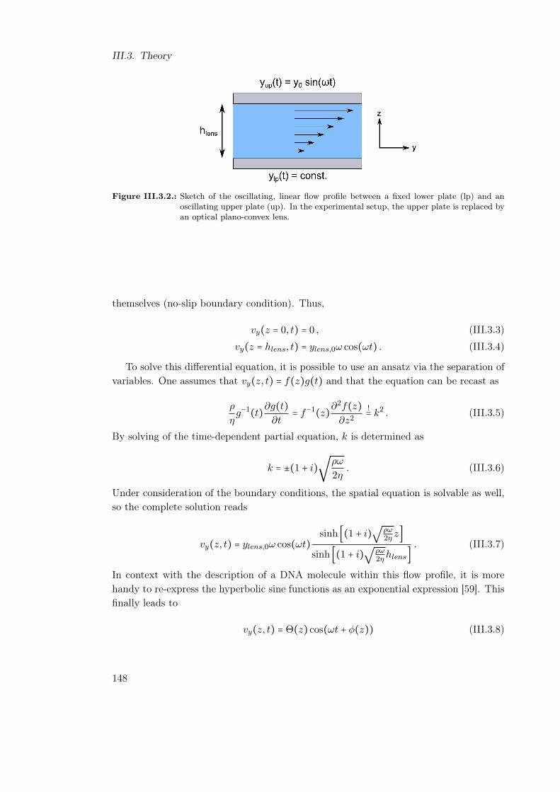
III.3. Theory
Figure III.3.2.: Sketch of the oscillating, linear flow profile between a fixed lower plate (lp) and anoscillating upper plate (up). In the experimental setup, the upper plate is replaced byan optical plano-convex lens.
themselves (no-slip boundary condition). Thus,
vy(z = 0, t) = 0 , (III.3.3)
vy(z = hlens, t) = ylens,0ω cos(ωt) . (III.3.4)
To solve this differential equation, it is possible to use an ansatz via the separation ofvariables. One assumes that vy(z, t) = f(z)g(t) and that the equation can be recast as
ρ
ηg−1(t)∂g(t)
∂t= f−1(z)∂
2f(z)∂z2
!= k2 . (III.3.5)
By solving of the time-dependent partial equation, k is determined as
k = ±(1 + i)√
ρω
2η. (III.3.6)
Under consideration of the boundary conditions, the spatial equation is solvable as well,so the complete solution reads
vy(z, t) = ylens,0ω cos(ωt)sinh [(1 + i)
√ρω2η z]
sinh [(1 + i)√
ρω2η hlens]
. (III.3.7)
In context with the description of a DNA molecule within this flow profile, it is morehandy to re-express the hyperbolic sine functions as an exponential expression [59]. Thisfinally leads to
vy(z, t) = Θ(z) cos(ωt + φ(z)) (III.3.8)
148

III.3.1. Flow Profile between Two Parallel Oscillating Surfaces
(a) Plot of the velocity amplitude Θ(z) at all positionsbetween the two plates.
(b) Plot of the phase shift φ(z) at all positions be-tween the two plates.
Figure III.3.3.: Dependence of the velocity amplitude and the phase shift of the moving fluid on theposition in z-direction between the plates. The position in z-direction is drawn on theordinate to facilitate a comparison with the sketch in figure III.3.2. The distance of theplates was fixed at 40µm for all calculations. The amplitude of the plate amountedto 30µm, while the frequency was set to three different values, indicated by differentcolors in the graphs.
with the amplitude
Θ(z) = ylens,0ω⎡⎢⎢⎢⎢⎢⎣
cosh (√
2ρωη z) − cos (
√2ρωη z)
cosh (√
2ρωη hlens) − cos (
√2ρωη hlens)
⎤⎥⎥⎥⎥⎥⎦
0.5
(III.3.9)
and the phase
φ(z) = arctan
⎡⎢⎢⎢⎢⎢⎣
tan (√
ρω2η z) tanh (
√ρω2η hlens) − tan (
√ρω2η hlens) tanh (
√ρω2η z)
tanh (√
ρω2η z) tanh (
√ρω2η hlens) + tan (
√ρω2η z) tan (
√ρω2η hlens)
⎤⎥⎥⎥⎥⎥⎦.
(III.3.10)
Thus, not only the amplitude of the flow profile depends on the position z between theplates, but also the phase shift φ. Since the phase shift of the DNA molecule relative tothe driving oscillation will play a crucial role later, a check should be performed whetherthe flow profile itself can cause a significant phase shift all by itself.
In figure III.3.3, the equations III.3.9 and III.3.10 are plotted for a fixed height ofthe lens as well as a given amplitude of the upper surface. The driving frequency wasvaried between 1Hz and 10Hz. When considering the amplitude, it becomes apparentthat the profile is completely linear if the phase is not considered. For the given distancebetween the plates and the given frequency range, the phase shift between the fluidmotion and the driving oscillation of the upper plate does also not play a significant role.
149

III.3. Theory
The biggest occurring phase shift always stays below 20mrad. Thus, for the parameterrange relevant for this work, no additional phase shifts need to be taken into account.This result facilitates the description of a DNA molecule attached to the fixed plate bya dumbbell model, which will be discussed in the following section.
III.3.2. Model for a Single-End-Grafted DNA-Molecule
As already explained in the introduction, one of the goals of this study is to find a simplemodel to describe the dynamic behavior of grafted DNA molecules. Quite a wide varietyof models has been used earlier to characterize them in certain flow situations. The Rouseand Zimmmodels are very popular when the extension behavior of the polymer is in focus,the Porod-Kratky model or worm-like chain model is preferred when the properties inthe freely floating or flowing state are an issue. However, since these options alreadyshow quite a high level of complexity, a much simpler model will be applied here.
The basic idea is sketched in figure III.3.4. When a DNA molecule is attached by somekind of bond to a cover slip, it typically shows a “mushroom”-like shape: A rather thinstem links the polymer to the cover slip. Above it, however, a big cloud containing mostof its mass floats. This has the particular consequence that the center of mass (COM ) ofthe molecule in average is situated at a certain distance z0 away from the cover slip. As aresult, instead of describing the DNA as a base-pair-wise bead-spring model, a reductiondown to two springs and a bead can be performed. A first spring attaches the COM atits average height z0 above the cover slip (not drawn in figure III.3.4b), a second onelinks it to the lateral center position directly above the grafting point. The polymeritself can be reduced to a bead with the same mass as the whole molecule. Its radius canbe modeled using the radius of gyration. In later experiments, the focal plane will bealigned parallel to the x-y-plane, thus, motion towards or away from the cover-slide willnot be visualizable. Since only the motion in this plane can be evaluated, hence, justone spring is depicted in the figure. During this modeling phase, the second spring will
(a) Single-end-grafted DNA moleculeson the surface of a cover slip.
(b) Simplified bead-spring model for the center ofmass motion of a DNA molecule in an oscil-lating linear shear flow.
Figure III.3.4.: Model system for single-end-grafted DNA molecules on a cover slip.
150

III.3.2. Model for a Single-End-Grafted DNA-Molecule
be taken into account, because it determines how far away from the lower cover slip theCOM is able to move and it will also determine how the occurring Brownian fluctuationswill be dampened.
Overall, if the model in the x-y-plane is considered, it consists of a spherical beadwhich is attached to a spring of a stiffness κ. The other end of the spring is grafted at adistance z0 away from the cover-slide. Although such a system cannot be realized in anexperiment without any complications, it will be very helpful in developing an analyticaldescription and a simulation of it. A flow oscillating in time created by a moving upperplate will be assumed. Due to advantages in analytic processing, the shear rate will beshifted by π/2 as compared to the past section and read γ(t) = γ0 sin(ωt). Since nonoteworthy additional phase contribution will occur because of the flow profile itself, thisshift will not play any further role at all. In context with optical tweezers, in section I.4.3a Langevin equation for a confined colloid was solved. Equation I.4.14 can be adaptedto be suitable for the motion of the grafted DNA molecule as well. It then reads
ζ∂z(t)∂t
+ κ(z(t) − z0) = Fr,z(t) , (III.3.11)
ζ (∂y(t)∂t
− γ(t)z(t)) + κy(t) = Fr,y(t) . (III.3.12)
Unlike the case involving optical tweezers, now, there is a shear-coupling between the z-and the y-direction, while no coupling is found to the x-direction. Just as before, thissystem of equations is solved by first tackling the z-direction via variation of variablesand then inserting the solution into the equation of motion in y-direction. That equationis solved by the same process. The solutions are given by
z(t) = z0 + e−t/τr⎧⎪⎪⎨⎪⎪⎩zs − z0 +
t
∫0
dt′Fr,z(t′)
ζet′/τr
⎫⎪⎪⎬⎪⎪⎭, (III.3.13)
y(t) = z0Wi1 + α2
{sin(ωt) − α cos(ωt)} (III.3.14)
+ e−t/τr {ys +Wi
α(zs − z0) (1 − cos(ωt)) + z0αWi
1 + α2}
+ e−t/τr⎧⎪⎪⎪⎨⎪⎪⎪⎩
t
∫0
dt′⎡⎢⎢⎢⎢⎢⎣et′/τr Fr,y(t
′)ζ
+ γ0 sin(ωt′)t′
∫0
dt′′ (et′′/τr Fr,z(t
′′)ζ
)⎤⎥⎥⎥⎥⎥⎦
⎫⎪⎪⎪⎬⎪⎪⎪⎭,
where α = ωτr is the dimensionless frequency and rs = (xs, ys, zs) is the initial startingposition of the bead. Similarly to before when a bead was confined in an optical trap, arelaxation rate is given by τr = ζ/κ. Since the solution for the y-direction depends on theWeissenberg number, the relative height z0/hlens is also included implicitly. This leads toa linear downscaling of the maximum displacement the bead can experience, depending
151

III.3. Theory
on the distance of the bead to the cover slip as well as the lens distance.In later experiments, the system will be observed using a very light-sensitive CCD
camera. The downside to this technique is that the recording rate is limited to 32Hz.In context with Brownian motion and stochastic molecular processes, this means thatall analytical considerations should be performed in the limit of long timescales. Hence,all terms included in the solution which depend on functions of the type exp(−t/τr) willdecay too quickly for visualization. Only those terms containing the Brownian force Fr,iwill be kept. The solution can be simplified to
z(t) t≫τrÐÐ→z0 + e−t/τrt
∫0
dt′Fr,z(t′)
ζet′/τr , (III.3.15)
y(t) t≫τrÐÐ→ z0Wi1 + α2
{sin(ωt) − α cos(ωt)} (III.3.16)
+ e−t/τr⎧⎪⎪⎪⎨⎪⎪⎪⎩
t
∫0
dt′⎡⎢⎢⎢⎢⎢⎣et′/τr Fr,y(t
′)ζ
+ γ0 sin(ωt′)t′
∫0
dt′′ (et′′/τr Fr,z(t
′′)ζ
)⎤⎥⎥⎥⎥⎥⎦
⎫⎪⎪⎪⎬⎪⎪⎪⎭.
Let us now leave the Brownian terms out of consideration as well. In this case, for they-direction only the first term remains. Just like in part I, equation I.4.35 can be appliedto it to obtain one single trigonometric function including a certain phase shift. It thenreads
y(t) = z0Wi√1 + α2
´¹¹¹¹¹¹¹¹¹¹¹¹¹¸¹¹¹¹¹¹¹¹¹¹¹¹¹¹¶ADNA(α)
sin(ωt−arctan(α)´¹¹¹¹¹¹¹¹¹¹¹¹¹¹¹¹¹¹¹¹¹¹¹¹¹¹¸¹¹¹¹¹¹¹¹¹¹¹¹¹¹¹¹¹¹¹¹¹¹¹¹¹¹¹¶δDNA(α)
) . (III.3.17)
When this displacement is compared to the driving by the oscillating lens, which is givenby ylens(t) = γ0
ω®
ylens,0
sin(ωt −π/2²δlens
), the phase shift between both of them can be defined as
∆δ(α) = δDNA(α) − δlens = −arctan(α) + π/2 . (III.3.18)
Based on the solution in equation III.3.17, two derived quantities can be defined. Thefirst one, also denoted as the relative amplitude, is gained by dividing the amplitudeADNA of the bead by the amplitude of the lens
Arel(α) =z0
hlens
α√1 + α2
. (III.3.19)
The second quantity is derived from the amplitude as well. By dividing equation III.3.19additionally by the relative height of the bead z0/hlens, the rescaled amplitude is gained
Aresc(α) =α√
1 + α2, (III.3.20)
152

III.3.2. Model for a Single-End-Grafted DNA-Molecule
(a) Dependence of the rescaled amplitude on the di-mensionless frequency.
(b) Dependence of the phase shift on the dimension-less frequency.
Figure III.3.5.: Results of the bead-spring model for DNA molecules. Analytical curves are shownin these semi-logarithmic plots as solid red lines, numerical data is presented in openblack circles.
which removes any dependencies of the amplitude on other parameters than the dimen-sionless frequency α. Both quantities will be a great benefit when analyzing experimentaldata later on.
In order to grasp the functional dependency of the rescaled amplitude within equationIII.3.20 as well as the phase shift within equation III.3.17 on the dimensionless frequency,both of them are plotted in figure III.3.5. Besides the analytic functions, also numericaldata is included which was gained by adapting the algorithm from chapter I.5 in the firstpart. According to both, the expected behavior of the rescaled amplitude will increaseproportionally to α for low frequencies α ≪ 1, i. e. ω ≪ τ−1
r . Upon exceeding α = 1, themaximum amplitude, which cannot be surpassed, is reached. To facilitate the explanationof this effect, let us go back to the sketch in figure III.3.4b. The maxmimum extensionof the spring, which is indicated in the figure and which leads to a perfect alignmentof the bead to the velocity front of the fluid, can only be reached at high frequencies.Otherwise, the spring succeeds in partially relaxing back to its equilibrium position andthus does not experience the full stretching.
The explanation for the behavior of the phase shift is a similar one. The drivingmotion is coupled to the motion of the bead via the flow velocity of the surroundingfluid. Hence, when comparing the phase of the displacement of the lens with the phaseof the bead displacement, at low frequencies α ≪ 1, both are shifted by π/2. This shiftthen decreases until α≫ 1. Then, it becomes zero and thus the bead directly follows themotion of the displaced fluid.
153

III.3. Theory
III.3.3. Summary
In the past chapter, a short introduction to the chemical as well as physical structureof DNA molecules was given. In total, it can be considered as a very long-chainedpolymer with a negative net-charge. In the scope of this thesis, λ-DNA, which consistsof roughly 50,000 base pairs and has a contour length of approximately 20µm when thedye-molecule YOYO-1 is intercalated, is utilized.
Since these molecules will later be attached to the surface of a cover slip and thensubjected to forced driving by oscillating a second surface, the resulting velocity profileneeded to be analyzed. This was performed in section III.3.1, where the correspondingNavier-Stokes equation was solved. The result, as figure III.3.3 shows, is a near-linearprofile that only deviates from the ideal case by a slight phase shift which depends onthe exact position between the oscillating upper and the resting lower plate. Since alloccurring phase shifts are quite small (δflow < 20mrad), it is not necessary to take theminto account during further analysis.
Afterwards, the DNA molecule was modeled as a bead which was linked by a spring tothe lateral position of the grafting point. The bead was identified with the center of mass(COM ) of the DNA, the stiffness of the spring represents the mechanical properties of themolecule. A second spring attached it to the height z0 within the channel. This heightcoincided with the typical distance of the COM of a grafted λ-DNA molecule. It wasdescribed analytically using a two-dimensional Langevin-equation, which also includedthe height-dependent shear coupling. Equation III.3.17 gives the simplified solution inthe limit of long times under negligence of the stochastic effects of Brownian motion.Basically, it consists of a sinusoidal response oscillation whose amplitude depends on thedimensionless frequency α, the average height of the COM z0, as well as the distanceof the lens hlens causing the driving. Moreover, a characteristic phase shift betweendriving and response oscillation which solely depends on the dimensionless frequencyaccording to the model is included. In the following chapter, this result will be comparedto experimental data sets and its validity will be checked.
154

III.4. Experimental Study
This chapter will focus on all elements that are required to perform experiments withsingle-end-grafted DNA molecules in an oscillating shear flow. On the one hand, a coverslip as well as the DNA need to be prepared. This process will be explained in the follow-ing. On the other hand, a specific setup using fluorescence microscopy is required, whichwill be described in section III.4.1. After acquiring picture series of bright, fluctuatingmolecules, their positions and especially their center of mass need to be determined. Asoftware built by André Schröder (Institut Charles-Sadron, Strasbourg, France) denoted“NEW Magneto” was utilized for this task (see Sect. III.4.2 for details). The performedexperiments as well as their results will follow in section III.4.3.
Before any experiments can be conducted, the DNA and a cover slip have to beprepared first. The general idea of this process is to use a streptavidin-biotin bond toattach the DNA to the cover slip. This kind of bond is one of the strongest non-covalent,biological bonds. Streptavidin is a protein produced by the bacterial species Streptomycesavidinii, biotin is better known as vitamin B7 or vitamin H. However, streptavidin comeswith the disadvantage of an isoelectric point between pH 6.8−7.5 which may vary withinthese bounds. Instead, for this study NeutrAvidin (ref.-no. A2666, Life TechnologiesGmbH, Darmstadt, Germany), which has its isoelectric point at pH 6.3 with no variation,was used. This helped to reduce non-specific binding.
To utilize this bond, the surface of the cover slip is treated with NeutrAvidin, whileeach DNA molecule is functionalized with a biotin molecule, which will be attached toeach other later on by bringing them in contact. This technique was introduced by Kootaet al. in 2007 [132] and has found a wide application since then [127, 131, 133]. However,both processes are not straight forward. λ-DNA are typically available in their circularstate as shown in figure III.4.1a. By a heat treatment, the ring has to be opened at twonicks, which leaves unbound overhangs with the sequences 5’-AGGTCGCCGCCC-3’ and5’-GGGCGGCGACCT-3’, one at each extremity of the molecule. Oligonucleotides withthe desirable functional group appended to them can now be bound to the DNA at thesepositions (Fig. III.4.1b). Quite a variety of functional groups like biotin, thiol, and manyothers are available. For the experiments presented here, a biotin- and a thiol-group werechosen. The biotin-group, as explained earlier, will be used for the grafting of DNA, whilethe thiol-group shows no interaction or binding to NeutrAvidin at all and is thus idealas a second functional group. In a final step, the backbone between DNA and oligomers
155

III.4. Experimental Study
(a) Circular λ-DNA. (b) DNA after tempering with biotinylated and thiolatedoligonucleotides marked with “B” and respectively “T”.
(c) DNA with both oligonucleotides bound to its extremities.
Figure III.4.1.: Ligation process of λ-DNA in preparation for single-end-grafting (drawing adaptedfrom [131]).
has to be repaired using a ligation reaction (Fig. III.4.1c). A more detailed descriptionof this process can be found in the appendix (Sect. A.2.3).
The second part of the preparation involves the cover slip. A NeutrAvidin layer asthin and homogeneous as possible needs to be brought on top. Again, a number of stepsis necessary to successfully reach this goal. They were adapted from the procedure byYuting Sun [131]. An step-by-step guide for the preparation is given in the appendix(Sect. A.2.4).
At this point, it is possible to attach the DNA molecules to the cover slip withoutrisking a collapse of the molecule or multiple attachment positions of a single DNA(comparable to the comic in Fig. III.3.4). However, in their current state, it is notpossible to visualize them. After all, the average radius of gyration is smaller than1µm with the single monomers on size scales of a few nanometers. Thus, before addingthe DNA molecules on the prepared cover slips, fluorescent dye molecules need to bebound to the DNA first. Quite a wide range of dyes has become available in the pastdecades. By now, they are widely accepted with their photophysical properties [134], theirfunction [135], and their mechanical properties [136] being well-researched. In this thesis,the intercalating dye YOYO-1 (ref.-no. Y3601, Life Technologies GmbH, Darmstadt,
156
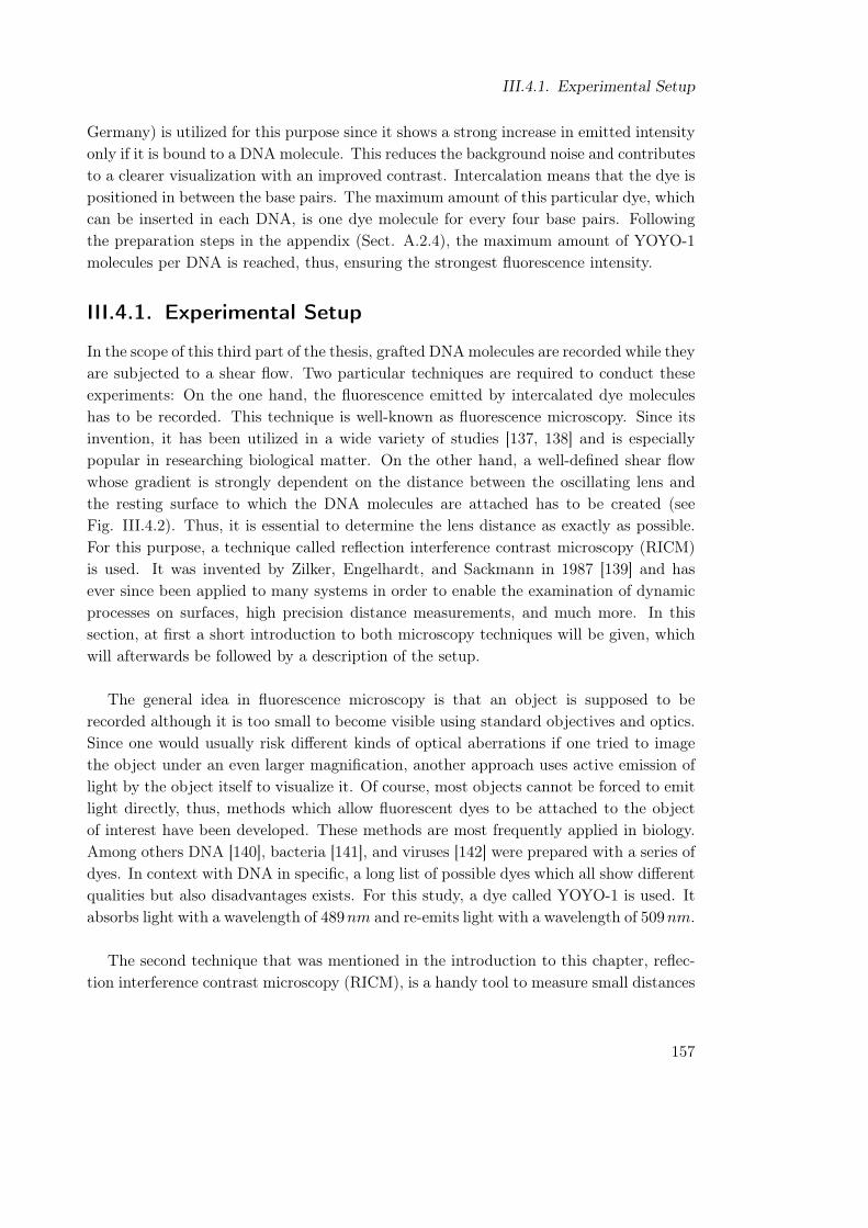
III.4.1. Experimental Setup
Germany) is utilized for this purpose since it shows a strong increase in emitted intensityonly if it is bound to a DNA molecule. This reduces the background noise and contributesto a clearer visualization with an improved contrast. Intercalation means that the dye ispositioned in between the base pairs. The maximum amount of this particular dye, whichcan be inserted in each DNA, is one dye molecule for every four base pairs. Followingthe preparation steps in the appendix (Sect. A.2.4), the maximum amount of YOYO-1molecules per DNA is reached, thus, ensuring the strongest fluorescence intensity.
III.4.1. Experimental Setup
In the scope of this third part of the thesis, grafted DNAmolecules are recorded while theyare subjected to a shear flow. Two particular techniques are required to conduct theseexperiments: On the one hand, the fluorescence emitted by intercalated dye moleculeshas to be recorded. This technique is well-known as fluorescence microscopy. Since itsinvention, it has been utilized in a wide variety of studies [137, 138] and is especiallypopular in researching biological matter. On the other hand, a well-defined shear flowwhose gradient is strongly dependent on the distance between the oscillating lens andthe resting surface to which the DNA molecules are attached has to be created (seeFig. III.4.2). Thus, it is essential to determine the lens distance as exactly as possible.For this purpose, a technique called reflection interference contrast microscopy (RICM)is used. It was invented by Zilker, Engelhardt, and Sackmann in 1987 [139] and hasever since been applied to many systems in order to enable the examination of dynamicprocesses on surfaces, high precision distance measurements, and much more. In thissection, at first a short introduction to both microscopy techniques will be given, whichwill afterwards be followed by a description of the setup.
The general idea in fluorescence microscopy is that an object is supposed to berecorded although it is too small to become visible using standard objectives and optics.Since one would usually risk different kinds of optical aberrations if one tried to imagethe object under an even larger magnification, another approach uses active emission oflight by the object itself to visualize it. Of course, most objects cannot be forced to emitlight directly, thus, methods which allow fluorescent dyes to be attached to the objectof interest have been developed. These methods are most frequently applied in biology.Among others DNA [140], bacteria [141], and viruses [142] were prepared with a series ofdyes. In context with DNA in specific, a long list of possible dyes which all show differentqualities but also disadvantages exists. For this study, a dye called YOYO-1 is used. Itabsorbs light with a wavelength of 489nm and re-emits light with a wavelength of 509nm.
The second technique that was mentioned in the introduction to this chapter, reflec-tion interference contrast microscopy (RICM), is a handy tool to measure small distances
157

III.4. Experimental Study
between microscopic objects. The principle of this technique is, as its name suggests,interference-based [143]. Light is sent through the microscope objective and then reachesthe sample cell. There it transmits through the cover slip and reaches the interface to afluid, typically water or a buffer solution. Due to a change in refractive index, this causesa partial reflection back towards the objective. If a second object lies in the path of thetransmitting beam, again, a certain amount of light is reflected. Since both reflectedbeams are optically retarded by a small amount in respect to each other, an interferencewhich depends on the distance of the object and the cover slip is caused. For point-likeor round objects, the interference appear in form of Newton rings, which periodicallymodify the intensity of the recorded light. However, for these rings to appear, the objectand the cover slip have to be in very close proximity. In other words, when measuringthe distance between the lens which will be used for driving the shear flow later and thecover slip carrying the DNA molecules, the appearance of these Newton rings signal thecontact between both of them. A micrometer screw can now be used to tune the distancebetween them as required.
For the application of both techniques, the same setup is used (Fig. III.4.2), which alsoallows the rapid switching between them. This has the advantage of allowing a quickdetermination of the distance of the lens, followed by the recording of a fluorescencepicture series without much loss of time. As a base, the inverted microscope Nikon
(a) Sketch of the key elements of the experimentalsetup.
(b) Photograph of the shear device above the micro-scope.
Figure III.4.2.: Representation of the experimental setup for shearing and visualizing the DNAmolecules.
158

III.4.1. Experimental Setup
Eclipse TE200 (Nikon GmbH, Düsseldorf, Germany) is used in combination with anoil immersion objective HCX PL Fluotar 100x RC by Leica (ref.-no. 11506199, Leica,Wetzlar, Germany). The objective has a numerical aperture of 1.3 and thus allowsto visualize a very broad field of view at a 100x magnification. As an illuminationsource, a mercury torch (HB-10104AF, Nikon GmbH, Düsseldorf, Germany) is attachedto the back port of the microscope. The visualization for the fluorescence as well asfor the RICM technique is realized using a very light sensitive 16 bit greyscale CCDcamera (ImagEM C9100-13, Hamamatsu Photonics Deutschland GmbH, Herrsching amAmmersee, Germany).
The most important part for the conduction of the experiments is a system whichallows to generate the necessary shear flows. This is realized by attaching an optical lensvia a spacer to a piezoelectric device (ref.-no. PX400 with amplifier ENV300, piezosystemJena GmbH, Jena, Germany). The lens (ref.-no. LA1576-A, Thorlabs GmbH, Dachau,Germany) has a low curvature radius rcurv = 6.2mm and is covered by an antireflexcoating for visible wavelengths. It allows to move the lens along one axis parallel tothe surface of the cover slip with the DNA molecules. Although an exactly parallelalignment of the piezo axis to the cover slip is a big challenge, any tilt over the verysmall displacement amplitudes used later is compensated by the curved surface of thelens and thus does not need to be taken into account. The assumption of flat parallelsurfaces in chapter III.3.1 is thus perfectly reasonable. The control over the displacementsof the piezo is conducted by a signal generator which is linked to the voltage input ofthe amplifier. This voltage signal is recorded synchronously to the picture series duringfluorescence microscopy via a National Instruments USB signal card (ref.-no. NI USB-6008, National Instruments, Austin, TX, United States of America). In order to beable to identify the measured voltage signals with displacements, a calibration of thepiezo device is performed by attaching fluorescing beads to the surface of the lens andvisualizing them using the fluorescence camera (Fig. III.4.3). A linear law becomesapparent, which is described by
Alens = 31.0(2) µmV
⋅Avolt − 0.4(1)µm, (III.4.1)
where Alens is the traveled distance in micrometers and Avolt is the applied voltage inVolts.
Especially in context with the analysis of oscillating signals and their relative phase,a precise timing of the recorded images is of the essence. In order to make sure that noadditional temporal delays need to be taken into account, we calibrated the recordingtimestamps of the camera with a known signal. This was performed by attaching acolloidal sphere to the surface of the lens which is coupled to the piezoelectric device asdescribed above. A sine signal of known amplitude and frequency was then applied to thepiezo device and recorded at the same time. This signal and its timestamp was compared
159

III.4. Experimental Study
Figure III.4.3.: Calibration curve of lens amplitude versus piezo voltage. The lens amplitude wasestimated by tracking attached fluorescing beads.
to the oscillations of the colloid. Overall, we found a signal delay of approximately30 ms between driving and response signal. This delay will be considered in all followingmeasurements by a corresponding shift of the timestamp of every image by −30 ms.
Depending on whether fluorescence excitation is used or whether an RICM measure-ment is of interest, a series of filters can be inserted. In RICM mode, the light is sentthrough a polarizer before it passes the objective, which is additionally equipped witha quarter-wave plate. An analyzer helps in enhancing the contrast before the light re-flected by the sample reaches the camera. In fluorescence mode, a combination of exciterfilter, dichroic mirror, and barrier filter is used (Nikon B-2A, Nikon GmbH, Düsseldorf,Germany). The exciter only allows a small band of visible light in the blue range be-tween 450nm and 490nm from the mercury torch to pass, which is then reflected by thedichroic mirror towards the sample. The fluorescent light from the YOYO-1 moleculesat 510nm then moves backwards through the objective and can also transmit throughthe dichroic mirror due to its design. The subsequent barrier filter blocks all excitationwavelengths from passing towards the camera and only allows the fluorescence light totransmit.
Since the camera is extremely sensitive to light, the “correct” amount of light dependsmainly on the recording frequency. If too much light arrives at the chip, all pixels displaythe brightest greyscale value and all details are lost. If, on the other hand, not enoughlight arrives, it is hard to make out any details since the contrast of the recorded images istoo weak. An ideal compromise would be a setting that shows the brightest pixels close tomaximum value while at the same time the background is as close to the darkest gray levelas possible. Neutral density filters (ref.-no. ND4 and ND8, Nikon GmbH, Düsseldorf,
160

III.4.2. Utilized Programs
Germany) help in reducing the incoming amount of light from the illumination source tolevels that can be visualized by the camera in a manner as optimal as possible. Anotherproperty that has to be taken into account is the fact that the fluorescence of YOYO-1bleaches after a certain amount of time. This means that, over the course of time, lessand less light is emitted, thus, there is a tight time limit to the measurements. If therecording should be performed over a longer amount of time, the intensity of the incidentlight can be reduced, which at the same time will reduce bleaching.
III.4.2. Utilized Programs
Nearly all necessary software for data evaluation was already mentioned in part I of thisthesis. Data handling and fitting was mostly conducted using Matlab and Origin. Beforethese tasks could be performed, the data sets had to be extracted from extensive pictureseries first. In general, they consisted of 512px × 512px wide areas containing brightspots, where the DNAs were attached to the cover slip. The COM of each moleculewas gained from each picture using the batch processing function of the software “NEWMagneto”. It had been written by André Schröder (Institut Charles-Sadron, Strasbourg,France) and provided all required options.
Typically, at first a region of interest (ROI) containing exactly one single DNAmolecule was selected. Additionally, a second ROI showing just the intensity backgroundrecorded by the camera was chosen. It was also possible to perform nearest-neighbor-filtering to reduce local intensity fluctuations and thus smoothen the evaluation of the
Figure III.4.4.: Comparison of originally recorded picture of grafted DNA molecules (Fig. A) andpost-processed picture after filtering (Fig. B). Oscillatory driving was applied to thesample cell (hlens = 40µm, Alens = 93µm, f = 1Hz) whose resulting effect is presentedin figures C to J. They contain snapshots of the following pictures with the filteringapplied to them. The region of interest (red circle) and a scale bar, both valid for allpictures, are marked in the first picture.
161
III.4. Experimental Study
picture. For all following data evaluations, the first neighboring pixels were taken intoaccount. As the next step, the software subtracted the average background intensityfrom all pixels and used a threshold value to determine which pixels actually contributedto the DNA molecule and which ones did not. The remaining pixels of interest were thenused to determine the COM of the DNA by weighting their position by the intensity
ri,COM =∑jri,jIj
∑jIj
, (III.4.2)
where i denotes the direction, i. e. x or y, and j is the index of a pixel. The result of thisimage processing is depicted in figure III.4.4. For each picture, the COM coordinateswere saved together with the time at which the picture had been recorded in a “*.txt”file.
In other situations, the analysis of the average image of a picture series was of interest.In this case, the software allowed to add all intensities over the whole series and to savethe resulting average image. This, for example, allowed the analysis of the densitydistribution of the polymer.
162

III.4.3. Measurements
III.4.3. Measurements
After the preparation of the samples has been finished, they are brought into the micro-scope. Typically, at first the desirable distance between lens and cover slip is set. This isachieved by bringing them into contact, which in RICM shows as Newton rings, and thenincreasing the distance via a micrometer screw. Then, the actual oscillation experimentsare performed, however, the lens distance is checked every few experiments in order toavoid too strong variations. The y-direction is always chosen as the oscillation direction.Three parameters have to be taken into account: the height of the lens, as well as theamplitude and frequency of the driving oscillation. The phase space of the experimentsis given by lens distances in the range between 40µm and 80µm, amplitudes between15µm and 140µm, and frequencies between 0.1Hz and 5Hz. However, not all combina-tions of parameters can be used since for smaller lens distances the amplitudes have tobe reduced to avoid damage to the DNA molecules like, for example, ripping.
After the evaluation of the COM of individual DNA as explained in the past section,displacement-time-curves as in figure III.4.5 result. There, the motion of the lens isdepicted as black symbols and the reaction of the COM is shown as blue symbols. Inthis case, it seems as if the DNA runs ahead of the lens motion. This is due to thecoupling of the COM motion to the velocity of the lens, which causes the additionalshift by π/2 (compare Sect. III.3.2). Both data sets can be approximated by a sinusoidalfunction with variable amplitude and phase shift, which then allows a comparison of both
Figure III.4.5.: Displacement-time-diagram of the lens (black circles) and the center-of-mass of a DNAmolecule (blue circles), as well as sinusoidal fits to both data sets (respectively col-ored, solid lines). The left axis corresponds to the data set of the lens, the right axiscorresponds to the DNA data. Driving at a lens distance of 60µm, an amplitude of107.7µm, and a frequency of 0.25Hz was applied to the system. The DNA COM isrunning ahead of the driving oscillation with a phase shift of approximately π/2 asexpected according to theory.
163

III.4. Experimental Study
(a) Auto-correlation function in x-direction. (b) Auto-correlation function in y-direction.
Figure III.4.6.: Auto-correlation functions of the motion of a DNA molecule under sinusoidal drivingat an amplitude of 30.9µm and a frequency of 5Hz. The lens distance is set to 60µm.
Figure III.4.7.: Histogram of the longest relaxation rates of the DNA molecules with a class widthof 56.5ms. Data was obtained by exponential fits to the auto-correlation functionperpendicular to the oscillation direction, i. e. the x-direction. The maximum of thedistribution is found at 442(8)ms, its average lies at 540 ms ± 350 ms.
oscillations.One further quantity in context with the analytical model in section III.3.2 is gained
by analyzing the auto-correlation functions of the COM motion: it is the longest relax-ation rate τr. Just as in part I, the LabVIEW VI presented in the appendix (Sect. C.1)is used for this purpose. As an example, in figure III.4.6 the auto-correlation functionsin x- and y-direction are shown. In the x-direction, after a quick relaxation process,which is well-described using a single exponential function, no characteristic correlationsignal is found besides noise and a weak oscillatory contribution due to an imperfectalignment. Since there is no shear- or similar coupling to the x-direction present in the
164

III.4.3. Measurements
system, this corresponds to the theoretical prediction. In oscillation direction, however,the exponential relaxation is superimposed by a strong oscillatory signal, which againcorresponds well to the theoretical assumptions. The desirable relaxation rate can nowbe determined by fitting an exponential function to the auto-correlation function Cxx.Due to the stochastic properties of the system, in this fashion not only one single ratebut a whole relaxation spectrum is determined by analyzing a series of DNA molecules(Fig. III.4.7). The histogram is described well by a Gaussian distribution whose leftflank is cut-off towards negative relaxation rates. The most frequently appearing ratecan be identified with the peak value at 442(8)ms. The average relaxation rate, though,constitutes 540 ms±350 ms. This average value will be used from now on throughout thischapter to determine the dimensionless frequency α. The relaxation rate determined inthis study exceeds the value of 400ms which was reported earlier by Doyle and others[124] by 35 %.
In the following, the experimental results from sinusoidal fits to the displacement datawill be compared to analytic results to check on the validity of the bead-spring model.According to equation III.3.17, the amplitude ADNA of the COM of the DNA dependson the dimensionless frequency α, the average height z0 of the COM, as well as the lensdistance hlens and driving amplitude Alens. If all parameters are kept constant exceptfor the lens amplitude, as illustrated in figure III.4.8 for four different frequencies, theCOM amplitude is supposed to depend linearly on Alens. This is indeed proven by theexperimental data since linear fits describe the curve progression well in all cases. Existing
Figure III.4.8.: Graph of the DNA COM versus the lens amplitude. The lens distance was set to40µm for all experiments, the frequency was varied from 0.1Hz to 0.5Hz as indicatedby color code. The dependence can be fitted using linear functions as illustrated bysolid lines.
165

III.4. Experimental Study
deviations are mostly due to Brownian fluctuations, additional background noise in thepicture series, and the misinterpretation of the contributions of certain pixels which door do not belong to the examined DNA molecule. No dependence of the phase shift onthe driving amplitude can be found, which is why no corresponding graph is shown inthis chapter.
Furthermore, the functional behavior of both the relative amplitude (Eq. III.3.19) andthe phase shift (Eq. III.3.18) can be checked in context with the lens distance. The modelassumes that the average COM height z0 does not change under any circumstances whenshear is applied to the system. When solving the differential equation (Eq. III.3.12) thishas the side effect, that the phase shift between driving and response oscillations doesnot depend on z0 at all, while the response amplitude ADNA shows such a dependence.When considering the relative amplitude in figure III.4.9a, a general decrease at each fre-quency is found for increasing distances. All of the curves can be fit with the analyticallypredicted behavior ADNA ∝ 1/hlens. To get a more robust estimation of the averageheight of the COM, one should consider the highest driving frequencies. In this case,according to the model, the COM completely follows the motion of the fluid and ADNAreaches a plateau value which is not influenced by an increase of the frequency. This wasdone in figure III.4.9a by adding the upper limiting envelope. It predicts the averageCOM height z0 to amount to 630nm. In case of the phase shift (Fig. III.4.9b), no cleardependence on the lens distance becomes apparent, although for frequencies higher than2Hz or respectively dimensionless frequencies higher than α = 6.8 there might be a weakeffect. It seems that for these higher frequencies, the phase shift decreases additionally in
(a) Plot of the relative amplitude Arel against the lensdistance. The black solid line marks the upper en-velope of all curves, defined by an average height ofthe COM of 630nm.
(b) Plot of the phase shift between driving and re-sponse oscillation as a function of the lens dis-tance.
Figure III.4.9.: Dependencies of the relative amplitude and the phase shift on the distance betweenoscillation lens and cover slip. The relations are shown in different colors for eachexamined driving frequency.
166

III.4.3. Measurements
a weak fashion when the lens distance is increased. However, the sinusoidal fits at higherfrequencies are more prone to errors and the effect might be due to a misinterpretationof DNA motion.
The most interesting functional dependencies are those of the relative amplitude andphase shift on the dimensionless frequency. The experimentally gained values for therelative amplitude are illustrated in figure III.4.10a. At each available distance, indicatedby different colors, Arel increases proportionally to α for α < 1. Upon exceeding α ≈ 1, aconstant plateau value is reached. This is equivalent to the maximum extension of theDNA molecule away from its equilibrium position which the linear velocity profile allows(compare Fig. III.3.4b). However, as fits with the analytical function (Eq. III.3.19) tothe data sets show, a good agreement with the experimental data sets is only found if amodification is applied to the fitting function. This modification allows small changes tothe critical frequency which marks the transition from the linear increase to the constantplateau. The fitting function reads
Arel(α) =z0
hlens
mα√1 + (mα)2
, (III.4.3)
where the lens distance is always fixed at the value in the corresponding experiment andm is the fudge factor for the frequency. For the fits in figure III.4.10a, this factor variesbetween 1.4 and 1.8 and thus indicates a small variation of the critical frequency. This
(a) Dependency of the relative amplitude Arel on thedimensionless frequency. Solid colored lines arefits to the open circle symbols colored respectivelyaccording to the model in equation III.4.3.
(b) Dependency of the rescaled amplitude Aresc onthe dimensionless frequency. The black solid linerepresents the analytical function where the di-mensionless frequency is multiplied by the factorm = 1.64.
Figure III.4.10.: Amplitude dependency on the dimensionless frequency. Relative amplitudes in subfig-ure III.4.10a are shown in subfigure III.4.10b after rescaling by the quotient z0/hlens.Both are drawn as log-log-plots.
167

III.4. Experimental Study
might be due to an underestimation of the average longest relaxation rate and wouldlead to a correction of the rate to a range between 620ms and 800ms. Overall, a goodtotal agreement of the amplitude behavior of the COM of the DNA molecules with themodel description is found. The average of all modifiers is found at the value m = 1.64
which will be used from this point on for rescaling the dimensionless frequency.If the relative amplitude in all curves is now rescaled by the corresponding relative
height of the center of mass z0/hlens, all curves shift on top of each other and can bedescribed by one master curve as given in equation III.3.20. It solely depends on thedimensionless frequency, which is mirrored by the results in figure III.4.10b. Again, avery good agreement to the analytical predictions (compare Fig. III.3.5a) is found.
The phase shift between the DNA COM and the displacement of the lens is plottedin figure III.4.11 as a function of the dimensionless frequency. According to theory, atlow frequencies a phase shift of π/2 which decreases with increasing frequency towards0 rad is to be expected. When this theoretical model (Eq. III.3.18) is compared to theresults from the measurements the predicted behavior is indeed found. However, just asin case for the amplitude behavior, the dimensionless frequency needs to be rescaled bythe factor m = 1.64 in order to give a more precise description of the functional behavior
∆δexp(α) = −arctan(1.64α) + π/2 . (III.4.4)
In case of the values at a lens distance of 80µm a slight overshoot towards negative
Figure III.4.11.: Dependency of the phase shift between driving and response oscillation on the di-mensionless frequency. The black solid line represents a fit with the theoretical model(Eq. III.3.18) where the dimensionless frequency was rescaled by the factor m = 1.64.A semi-logarithmic scale was chosen.
168

III.4.3. Measurements
phase shifts is observable. In this case the large error bars should be considered as well,though, which still indicate agreement with the model. Over the whole observable fre-quency spectrum, the assumed bead-spring model seems to capture the amplitude as wellas the phase behavior of the center of mass in a perfect manner under the assumptionof an effective dimensionless frequency αeff = 1.64α. It is, hence, suited very well as adescription of single-end-grafted molecules in a linear, oscillating shear flow.
There is an alternate way to evaluate the displacement of the DNA molecule. However,dynamic changes to the system cannot be captured by it. Instead of tracking the COMof each molecule, it is possible to measure the length of each DNA in an average imageover a whole picture series. The calculation of these averages is also a feature of “NEWMagneto” and can be performed with ease. By choosing a region of interest parallel tothe oscillation axis along the molecule, for small amplitudes, the intensity profile will beidentical with a Gaussian distribution. For bigger amplitudes, this curve will broaden andfinally form two separate maxima at the reversal points of the oscillation. Since the overallamplitudes are quite small, a Gaussian fit to the intensity distributions is reasonable inall cases. The standard deviation of the curves can be used as a comparative value tothe amplitudes of the oscillations of the center of mass. The result for a lens distanceof 40µm is displayed in figure III.4.12. There, the amplitudes deduced from the sinefits are shown (black circles) together with the results from the length evaluation of theintensity profiles (red circles). Additionally, three data points at even higher frequencies(f = 10/20/32Hz), which were recorded at a picture acquisition rate identical to theoscillation frequency at a lens distance of 60µm, are displayed. Thus, it is not possible,in case of these measurements, to make out any details about their amplitude or phasebehavior. In other words, the sine fit evaluation is not possible. However, the lengthevaluation can be conducted and the respective oscillation amplitudes can be estimated.
A property that can be deduced from figure III.4.12 straight away is that, for lowdimensionless frequencies below α = 10, the sine fit and length evaluations both givethe same qualitative behavior, although there is a deviation in absolute value. This isprobably due to the fact that the standard deviation of the Gaussian curves cannot bedirectly identified with the amplitude of the COM. However, this only causes an offset ofboth curves relative to each other and can be corrected by a calibration. The qualitativeagreement between both methods is lost, though, when the frequencies are increasedabove α = 10. There, the length evaluation shows much bigger relative amplitudes thanthe sine fits do. The fact that the high frequency oscillations were performed at a biggerlens distance should in fact not cause an increase in relative amplitude, but rather theopposite. This is of course only true if the bead-spring model is trusted as a suitabledescription. This will also be open for discussion in the following chapter.
Much care has to be taken when considering the robustness of those data sets. Toillustrate this, the absolute length of the intensity profiles from the averages is compared
169
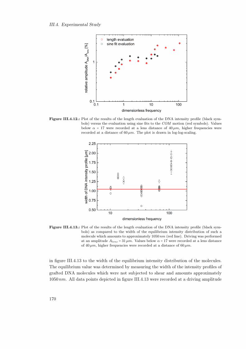
III.4. Experimental Study
Figure III.4.12.: Plot of the results of the length evaluation of the DNA intensity profile (black sym-bols) versus the evaluation using sine fits to the COM motion (red symbols). Valuesbelow α = 17 were recorded at a lens distance of 40µm, higher frequencies wererecorded at a distance of 60µm. The plot is drawn in log-log-scaling.
Figure III.4.13.: Plot of the results of the length evaluation of the DNA intensity profile (black sym-bols) as compared to the width of the equilibrium intensity distribution of such amolecule which amounts to approximately 1050nm (red line). Driving was performedat an amplitude Alens = 31µm. Values below α = 17 were recorded at a lens distanceof 40µm, higher frequencies were recorded at a distance of 60µm.
in figure III.4.13 to the width of the equilibrium intensity distribution of the molecules.The equilibrium value was determined by measuring the width of the intensity profiles ofgrafted DNA molecules which were not subjected to shear and amounts approximately1050nm. All data points depicted in figure III.4.13 were recorded at a driving amplitude
170

III.4.3. Measurements
of 31µm in order to allow a quantitative comparison among them. At α = 10, the widthof only one of the sheared DNA molecules lies below the equilibrium value. All othervalues for α < 17 are situated above this threshold. The same is true for all values thatwere recorded at α = 109. However, a significant amount of values at α = 34 and α = 68
show a smaller width of the intensity profile under shear compared to the equilibriumthreshold. Thus, the significance of these data sets must be questioned in terms of theirvalidity. Overall, the presented data sets in figures III.4.12 and III.4.13 can be consideredto be robust up to α = 17 or respectively f = 5Hz.
171

III.4. Experimental Study
III.4.4. Summary
The past chapter contained a detailed description of all elements that are related to ex-periments with single-end-grafted DNA molecules. At first, the general idea of attachingone extremity of DNA molecules in a reproducible manner to a cover slip was explained.A detailed preparation recipe is given in the appendix (Sect. A.2.3 and A.2.4).
Although λ-DNA is a fairly long-chained molecule with a total length of about 20µm
in its fully stretched state, its structures are still much too small to visualize them by stan-dard optical microscopy. Instead, a setup using fluorescent excitation of dye moleculeswas necessary. During the shear experiments, a means was also required to determinethe distance between the moving and the resting surface. This could be achieved usingreflection interference contrast microscopy (RICM). Both techniques were explained insection III.4.1, as well as the experimental setup necessary to conduct them. There, therealization of the shear device was explained as well.
After the conduction of a shear experiment, picture sequences which showed manyfluctuating bright spots resulted. The position of the center of mass (COM ) of each ofthe molecules had to be extracted from the pictures before a further analysis was possible.A custom-built piece of software which was very helpful in that regard was described insection III.4.2.
In section III.4.3, the performed shear experiments on grafted DNA molecules werepresented and partially discussed. A comparative analysis with the analytical bead-springmodel showed very good agreement for both the relative amplitude (Fig. III.4.10) andthe phase shift between driving lens oscillation and COM response oscillation becomesapparent (Fig. III.4.11). However, in both cases, the dimensionless frequency α neededto be replaced by an effective dimensionless frequency which was shifted in respect toα by a factor of 1.64. By performing an alternate evaluation of the amplitude behaviorwhich took the length of the average intensity profiles into account instead of the dy-namics of the COM, at low frequencies, the same qualitative development was found. Athigher frequencies, strong deviations began to occur, though. A discussion of the possiblereasons for these discrepancies will follow in the next chapter.
172

III.5. Discussion
The third part of this thesis deals with single-end-grafted DNA molecules that are sub-jected to an oscillating shear flow. In chapter III.3, a strongly simplified model whichdescribed each DNA via its center of mass was developed. It was then modeled as abead with the same total mass as the molecule and with a radius that is identical to theradius of gyration of the polymer. In order to take the attachment point at the cover slipinto account, the motion of the center of mass (COM ) was restricted by linking it to anequilibrium position placed above the grafting point with a spring. In chapter III.4, theanalytical predictions by the model were compared to results from experiments whichwere gained by fluorescence microscopy. Two central features were analyzed: On the onehand, the frequency dependence of the amplitude of the COM is an interesting topic, onthe other hand, the phase shift between driving and response oscillations is importantas well. Thus, in this chapter, the amplitude and phase behavior of the model shall bediscussed.
Let us begin by considering the relative or, respectively, the rescaled amplitude. FigureIII.4.10b shows that for all lens distances, the dependency of the relative amplitude onthe dimensionless frequency is described well by the bead-spring model. However, itwas mentioned before that, in order to achieve this agreement, the frequency needs tobe rescaled by a pre-factor as presented in equation III.4.3. Before the addition of thispre-factor, the position of the transition value of the frequency at α = 1 seemed to haveslightly too small a value. The pre-factor m, which in all experiments amounted between1.4 to 1.8, allows the shift of this transition frequency, such that a better agreementbecomes possible. In average, it amounts to the value m = 1.64. A probable reasonfor the false estimation of the transition frequency lies in the misinterpretation of pixelvalues. Either pixels which do not belong to the DNA molecule were included in thecalculation of the COM or pixels which should have been included were left out. This isa general problem of the evaluation of a picture series relying on a threshold value, be it adynamically adapted threshold or a static one. Under any circumstance, the bead-springmodel and the experimental values agree to a very high degree as far as the relativeamplitude is concerned, thus, the model can be trusted to reflect the actual behavior ofthe DNA.
An alternate evaluation method was applied to the data sets, in which the length of aDNA molecule was considered by analyzing the average image over all pictures recorded
173

III.5. Discussion
in a measurement and thus over multiple oscillation periods of the DNA. For dimension-less frequencies α < 10 a reasonable agreement to the relative amplitude values from thesine fits is found (Fig. III.4.12). For higher frequencies, a clear overshoot results from thelength evaluation. The reasons for this effect are so far unclear, especially since the threehighest frequencies at α = 34/68/109 were recorded at lens distances of 60µm and not at40µm like all other data points shown. Bigger lens distances result in smaller relativeamplitudes at the same frequency value as figure III.4.10a depicts, which is exactly thecontrary of what is the case for the alternate evaluation. One additional aspect thathas not been discussed yet needs to be considered. For many picture series among thesehigh frequency measurements, it seems that the DNA molecules are not only attachedat their functionalized extremity, but they also temporarily adsorb to the cover slip atsome point along their backbone. This can be seen as a kind of unspecific interaction,which in total leads to a shorter segment of the DNA molecule following the oscillatorydriving, while the rest of it remains stuck to the cover slip in a stretched state. Thisagain leads to what looks like a more elongated molecule and thus to an overestimationof its length. These adsorption processes, however, only start to play a role if the drivinghappens at dimensionless frequencies larger than α = 17.
If the phase shift is considered, the bead-spring model predicts a decrease startingat π/2 for low frequencies, which then drops towards 0 rad at high frequencies. Thisspecific behavior is indeed found over the whole accessible frequency spectrum for 0.1 Hz ≤f ≤ 5 Hz or respectively 0.3 ≤ α ≤ 17 (Fig. III.4.11). However, as mentioned above,the functional behavior is captured in a more precise manner when using the effectivedimensionless frequency αeff = 1.64α instead of α for the description of the phase behavior.
When examining the phase shifts at different lens distances, it seems as if ∆δ getssmaller the bigger the lens distance is. In other words, the smallest value of approxi-mately −0.34 rad is reached for a lens distance of 80µm, while it amounts to 0.07 rad
at the same frequency in case of a lens distance of 40µm. Since all oscillation processeshappen very fast and due to the small amount of light depicted by each image in eachpicture series, it is a very challenging task to grasp the oscillatory behavior. However,as already mentioned, it is not an easy task to distinguish between those bright pixelsbelonging and those not belonging to a certain DNA molecule. Additionally, the smallnumber of pictures and thus also COM displacement values in each oscillation periodat high driving frequencies makes the exact determination of the correct amplitude andphase values of the DNA oscillations a challenge as well. This is also a possible reason forthe phase shift overshoot in the data set for h = 80µm. This is also the reason why thesize of the error bars in the fits increases with increasing frequency. Overall, there mightbe a hidden dependency of the phase shift on the lens distance which only seems to play arole at high driving frequencies. At the current state of technology, an in-detail mappingof the high frequency range above α = 17 is hindered by a wide number of experimental
174

(a) Behavior of the relative amplitude of the DNACOM (Fig. 2.44 in [127]).
(b) Behavior of the phase shift (Fig. 2.46 in [127]).
Figure III.5.1.: Results of the experimental study of M. Khaksar with single-end-grafted DNA [127].Blue crosses indicate measured data points, while the solid red line represents thecorresponding prediction by the analytical model.
issues. In the following chapter, a series of improvements and other changes which mighthelp in enabling high frequency measurements will be mentioned.
As a final topic of discussion, the results which were gained in scope of this thesisshall be compared to those results reported earlier by Maryam Khaksar [127]. Two of hercentral graphs, which show the dependency of the rescaled amplitude and the phase shifton the dimensionless frequency, are depicted in figure III.5.1. In case of the amplitude, adistinct peak at α = 2 is apparent. She identified this feature as the strongest deviationfrom the assumed bead-spring model, which is identical to the model used in this thesis.Furthermore, she assumed that it was either related to the internal energy landscape ofthe DNA or a specific dynamic response function. If, indeed, a peak is present at thisposition, even a resonant response of the DNA molecule would be a possible explanation.When compared to the rescaled amplitude from this study depicted in figure III.4.10b,no such peak appears, though. The rescaled amplitude follows the analytical modelover the whole examined part of the frequency spectrum. Even multiple repetitions ofher measurements did not show any similar feature. Thus, one might argue that thepeak in her results originated from a different source like for example external noise or amisinterpretation of the picture series.
Let us consider her results of the phase shift between the driving and response oscilla-tion of the DNA COM in figure III.5.1b. Here, it becomes apparent that for frequenciesα < 1 she found a good agreement between her measurements and the predictions bythe model of the dampened harmonic oscillator. However, for higher frequencies, shereported significant deviations from the model which are characterized by an overshoot
175

III.5. Discussion
towards negative phase shifts and large error bars. In other words, her phase analysisresults in a nearly identical curve progression of the phase shift that was also found inthis study (Fig. III.4.11). It has to be kept in mind that her analysis of the frequencyspectrum above α = 1 only consists of four values, the last of which shows a significanterror (> ±0.5 rad). If the negative phase overshoot is considered as significant it maymean that in case of both experiments similar difficulties in performing the measure-ments were met and that improvements are required in order to be able to realiablyresolve the motion of DNA at higher frequencies. Both setups contain the identical sheardevice, both of them are mounted on top of an inverted microscope. Also, the majorpart of the sample preparation and the lab environment were similar, hence, a similareffect on the conduction of the experiments can be assumed.
Since the plot of the phase shift in Maryam Khaksar’s thesis does not allow a dis-tinction of the phase shifts at different lens distances, a more detailed comparison of theresults is not possible. However, the partial agreement of both studies casts an interestinglight on the mechanical properties of single-end-grafted DNA molecules.
176

III.6. Summary
In this part of the thesis, the mechanical properties of single-end-grafted DNA moleculeswere under examination. More specifically, by attaching single DNA molecules to thesurface of a cover slip, their motion could be restricted to a small region of interest.At the same time, their mechanical properties were mostly uninfluenced and even theirdynamical behavior could be visualized.
The challenge was two-fold: From an experimental point of view, the DNA moleculesneeded to be grafted to the cover slips and a series of shear experiments were to beperformed with them. From a theoretical point of view, a model which allowed theinterpretation of the behavior of the molecules and enabled predicting the response tocertain excitations had to be developed. The results of the analytical considerations werepresented in chapter III.3, where at first the flow profile between an upper oscillating anda lower resting plate was calculated by solving the corresponding Navier-Stokes equationof motion. The results predicted that for typical oscillation frequencies and amplitudesof the shear device, a linear velocity profile which only showed a very weak phase shiftof fluid motion when comparing the fluid motion at the surface of both plates could beexpected. Thus, the phase shift can safely be ignored and a perfectly linear velocityprofile can be assumed in all cases. This result then led to the development of a bead-spring model for grafted DNA molecules (Sect. III.3.2), which could be described by atwo-dimensional Langevin equation. After a series of simplifications, the motion of thecenter of mass of a grafted polymer driven by an oscillating top plate was given by aphase-shifted sine-function (Eq. III.3.17). Both the phase shift and the amplitude of theresponse were dependent on the driving frequency, however, the amplitude additionallydepended on the average distance between the center of mass and the lower plate, thedistance to the upper plate, as well as the amplitude of the driving oscillation. Thisanalytical result could also be verified by numerical simulations (Fig. III.3.5).
For the experimental observation of λ-DNA (Ch. III.4), an existing preparation pro-tocol by Yuting Sun [131] which enabled the functionalization of the cover slip withNeutrAvidin, a streptavidin derivate with a different isoelectric point, and of the DNAmolecules with biotin was adapted. When brought into contact, the DNA tended to at-tach itself with its biotinylated extremity to the cover slip, while the rest of the moleculeremained unconfined and could react to changed flow conditions. A whole series of expe-riments was performed with the polymers in section III.4.3 involving different distancesbetween oscillating and resting surface, as well as a variation of driving amplitudes and
177

III.6. Summary
frequencies. When taking the behavior of the response amplitude of the DNA into account(Fig. III.4.10), the predicted curve progression was recovered to a very exact degree. Thesame is true for the phase shift between driving and response oscillation (Fig. III.4.11).In some cases though, at frequencies above α = 6, an overshoot towards negative phaseshifts became apparent. Probably, this is due to imprecision during the image analysisand insufficient lengths of the recorded data sets which hence cause significant fittingerrors. A similar behavior was already recovered two years ago by Maryam Khaksar[127], a detailed comparison and discussion of the results was conducted in chapter III.5.
There are a few changes and improvements which are desirable for future studies inthis field. If possible, the setup should be modified in such a way that noise can bereduced further and image series can be recorded with an improved contrast. This wouldhelp immensely in evaluating the contribution of certain more or less bright pixels tothe center of mass calculation and thus give a clearer result especially at high drivingfrequencies. This directly leads to another improvement: A camera which supports aneven higher recording frequency at a similar or even better sensitivity would help inexpanding the experimentally accessible frequency spectrum. This would give insightinto the behavior of DNA molecules at even higher driving frequencies and thus maybecontribute to answering the question whether the currently utilized bead-spring modelis sufficient in describing the dynamic properties of the system. If, afterwards, it shouldstill be necessary, a more complex model for the system could be developed. So far,it is largely unsettled what such a model might look like since no clear picture of thereaction of the DNA molecules to a faster driving can be drawn yet. A first step mightbe the expansion of the model of the dampened harmonic oscillator to include additionalrelaxation rates of the polymer.
In total, although still many open questions exist in context with single-end-graftedDNA molecules, insight was gained into their mechanical behavior. So far, most studiesfocused on properties of non-attached molecules [125] or they examined the static elonga-tion under a steady instead of an oscillating shear flow [124]. Experimental observationof DNA molecules in flows is a very challenging task since many preparation steps arerequired before such studies become feasible in the first place. Although much moresophisticated models for DNA molecules already exist and were applied successfully inthe past, their modeling as beads linked to a spring was attempted. And even thoughthe model is as simple as it can be, for the most part, the response of the molecule can bedescribed fairly well. However, some open questions remain like for example the questionof the significance of negative phase shifts at high frequencies. Finding the solution tothese will be the quest for future studies.
178

Summary
179


In this study, Brownian motion of colloids or colloid-like systems in oscillatory fieldswas examined. Three different systems were investigated: In part I, a colloid was con-fined by an optical trap within a shear flow and then subjected to oscillations by movingthe optical trap. In part II, the identical setup of optical tweezers was utilized in orderto probe respiratory mucus of horses with colloidal particles. This was conducted byanalyzing both passive Brownian motion as well as active oscillations of the colloid inthe mesh of the material. Part III gave details about the study of DNA molecules whichwere attached to the surface of a coverslip while being subjected to an oscillating shearflow.
The idea behind the study in part I was to find out how the shear-induced coupling ofBrownian motion in a shear flow would be influenced if external oscillations were added tothe system. This was achieved experimentally by combining the use of a setup of opticaltweezers with a gravitationally driven microfluidic device. In case of stochastic systemsinvolving Brownian motion, such coupling effects are accessible well by considering auto-and cross-correlation functions of the motion in flow direction and perpendicular to it,i. e. in direction of the shear gradient. Thus, we decided to approach the analysis of oursystem by the help of correlation functions as well. This approach included the analyticsolution of the Langevin equation of motion for the colloid and the determination of theanalytic auto- and cross-correlation functions. These were afterwards compared with theresults of a numerical study basing on the same differential equation as well as experi-mental results gained in our setup of optical tweezers.Overall, we found an analytic solution to the Langevin equation including the respectivecorrelation functions. These solutions were reproduced by the numeric study and alsodisplayed the characteristics found in the experimental study. However, we experiencedsignificant perturbations which hinder the successful conduction of such experiments.There were two perturbations which were considered the most important ones: Theframe of reference misalignment of the recording device, i. e. the high-speed camera,used to visualize the motion of the confined colloids led to an undesirable coupling ofthe motion in flow- and gradient-direction and hence caused spurious correlations. Evenmore important were temporal fluctuations of the flow velocity which contradict the as-sumption of a stationary flow in the theoretical part of this study. Thus, although theexamined system was built as simple as possible the results can be considered inconclu-sive. However, suggestions were made which may help in improving the setup for furtherstudies and hence lead to more conclusive results.
In part II, the setup of optical tweezers and a cone-and-plate rheometer were utilizedto study the rheological behavior of mucus. This did not only lead to the discovery ofrich viscoelastic response properties of this material but also revealed a clear gap betweenthe microscopic and the macroscopic response. As a comparison the Mori-Tanaka model
181

was applied which is typically used to describe rigid foams. These are characterized bytwo separate phases, a solid-like phase which forms the walls of the foam and a viscousphase which fills the pores between these walls. While in microrheologic experimentswith optical tweezers the colloid for the most part only “feels” the viscous phase, in caseof the macrorheologic experiments with the rheometer the whole continuum includingboth phases is probed. Thus, in that case, the elastic material properties play a muchmore significant role. Partially, the results of this study were already published earlier[76].
In part III of this study, DNA molecules were studied in a similar flow situation as thecolloids in part I. One extremity of these molecules was attached to a surface while theremainder of them stayed afloat in a buffer medium. By driving the surrounding mediumwith external oscillations originating from a second surface attached to a piezoelectricdevice, the response behavior of the DNA was examined. As free parameters, the distancebetween both surfaces, the amplitude of the driving oscillations and their frequency werevaried. We analyzed the displacements of the DNA center of mass and observed thedependence of its amplitude and phase behavior on the driving frequency. A surprisinglygood agreement with the model of a dampened harmonic oscillator was found. However,we observed a shift of the characteristic relaxation rate intrinsic to the model as comparedto the one determined during our experiments. We assume that this effect might becaused by the complexity of a DNA molecule and hence the fact that one single relaxationrate probably does not suffice in order to describe the full dynamic behavior of such amolecule.
182

Part IV.
Appendix
183


A. Materials & Methods
A.1. Materials
name manufacturer vendor art.-no.3-aminopropyltriethoxysilane The Dow Chemical Sigma-Aldrich 440140(APTES) Company
Gene Frame 25µl ABgene Ltd. Fisher Scientific AB-0576GmbHglutaraldehyde, EM Grade, 8 % Polysciences, Inc. 00216
λ-DNA Fermentas Fisher Scientific SD0011GmbHmelamin resin beads Fluka Sigma-Aldrich 90641size: 5µm
Microcon DNA Fast Flow Merck Millipore MRCF0Centrifugal Filter Unit R100
NeutrAvidin Molecular Probes Life Technologies A2666GmbHoligonucleotides MWG Biotech n/aphosphate buffered saline (PBS) Sigma-Aldrich P4417
polyacrylamide (PAAm) Sigma-Aldrich 92560polydimethylsiloxane The Dow Chemical Sigma-Aldrich 761036(PDMS) Sylgard 184 Companypolymethylmethacrylate Fluka Sigma-Aldrich 73371(PMMA) beads, size: 4µm
T4 DNA ligase New England Biolabs M0202S
YOYO-1 iodide (491/509) Molecular Probes Life Technologies Y3601GmbH
Table A.1.: Chemical products and microparticles utilized to conduct the experiments in all parts ofthis thesis.
185

A. Materials & Methods
A.2. Methods
A.2.1. Production of Microfluidic Devices
In chapter I.4.2, the design aspects of a microfluidic device with channels of rectangularcross-section were described. Before the conduction of each experiment, one of thesedevices had to be produced. The protocol is as follows:
1. As polydimethylsiloxane (PDMS) material Sylgard 184 (ref.-no. 761036, Sigma-Aldrich, Germany) containing elastomer base and a curing agent is used. Both ofthem are mixed in a 10:1 base to curing agent volume ratio inside a small mixingglass bottle. The total volume may vary depending on the surface area of themicrofluidic device. It should be chosen so that the height of the poured PDMS-layer will be about 5mm high. The mixture is stirred by hand for half a minuteusing a disposable plastic stirrer.
2. The bottle is brought into a vacuum reactor and degassed until no air bubbles areleft.
3. The mixture is poured onto the silicon wafer with the negative structures of themicrofluidic device which rests inside a plastic dish. Afterwards, the dish is closedwith a lid in order to avoid the inclusion of dust.
4. The dish is brought into a pre-heated oven at a temperature of 65○C and leftinside for one hour. It is taken out afterwards and passively cooled down to room-temperature.
5. The device is generously cut out of the mold using a scalpel and carefully pealedout of the plastic dish. Special care has to be taken not to bring the device incontact with dust. This is best performed inside a flow-box.
6. Holes for the in- and outlet tubes are punched into the PDMS using a syringewith a blunted tip and the device is put upside-down with the channel structurespointing upwards in an O2-plasma-cleaner together with a microscope coverslip bigenough to cover the whole area of the PDMS device. It is exposed to the plasmafor about one minute.
7. The side of the PDMS with the structures of the microfluidic channels and theactivated side of the coverslip are oriented pointing towards each other and thencarefully brought into contact.
8. The in- and outlet tubes are inserted into the holes of the device.At this point, the microfluidic device is ready for use. Tubes made from polyethylene(LDPE) with an inner diameter of 0.5mm and an outer diameter of 1mm were used(art.-no. 3550501, Laborshop24, Gross-Zimmern, Germany).
186

A.2. Methods
A.2.2. Preparation of Gene Frames for Microrheology Experiments
In context with the microrheological examination of mucus or biological fluids in general,in section II.4.1.2 a special low-volume sample cell denoted Gene Frame was mentioned.Here, the specific preparation steps of the cell will be detailed. A package of Gene Framescontains two items: the adhesive frame and a plastic cover slip. The adhesive has theshape of a square with a 1 cm×1 cm hole in the middle, its thickness amounts to 250µm,thus defining a volume of 25µl. The preparation steps are as follows:
1. A standard cover slip is cleaned using two rinsing steps with acetone and ethanol.The ethanol is afterwards removed using compressed air.
2. The adhesive frame is aligned over the surface and attached to it by pressing itdown gently. To improve the adhesion, the cover slip is heated for about 5 minutesto 94 ○C.
3. The back cover of the adhesive frame is now removed to expose the inner volume.The respective amount of sample fluid is pipetted into it.
4. The plastic cover slip from the Gene Frame package is now carefully aligned overthe adhesive. It should be attached at one side of the frame first, then bent andslowly rolled over the whole adhesive surface. In this way, air inclusions in thesample volume can be avoided. Also, excess fluid is pushed out of the frame.
The sample cell is now ready for use.
A.2.3. DNA preparation
λ-DNA molecules have to be prepared before they can be attached to cover slips. In theirdelivery state, they are available in circular form. This form needs to be linearized andfunctionalized using oligonucleotides with certain molecules like biotin, thiol, or othergroups appended to them. To achieve this, the following recipe originally suggested byYuting Sun [131] was used:
1. 66µL λ-DNA at 0.5µg/µL is pipetted into an Eppendorf tube and heated to 75○Cfor 10 to 15 minutes to open the circular DNA. This step is followed by a quickcooling process down to room temperature for about 5 minutes using ice.
2. 10µL ligase buffer, 3.4µL oligomer 1, 3.4µL oligomer 2, and 17.2µL Milli-Q waterare added to the tube to give a total volume of 100µL. Oligomer 1 and 2 can bechosen as necessary for the experiments, they have to be complementary to each ofthe two base sequences finalizing the DNA molecules. For the experiments in partIII, a biotin and a thiol group were chosen as the corresponding functional groups.
3. The hybridization of the DNA is performed by heating the sample to 50 ○C andkeeping the temperature constant for about 1 hour.
4. A slow tempering process down to room temperature is performed over night byswitching off the heating unit.
187

A. Materials & Methods
5. 3.4µL T4 ligase are added to the sample to close the gap in the backbone betweenthe DNA molecule and the oligonucleotides. For this purpose, the sample is heatedto 25 ○C for approximately 30 minutes.
6. The sample is then purified by filtering it five times through special filters (ref.-no.MRCF0R100, Microcon DNA Fast Flow Centrifugal Filter Unit, Merck Milipore,Darmstadt, Germany) using a centrifuge at very low rotation velocities (150 rcf).
All materials are listed in table A.1. After these preparation steps, the DNA solution issplit into multiple aliquots of ≈ 20µL within Eppendorf tubes and afterwards frozen at−80 ○C until they are needed.
A.2.4. Preparation of a cover slip and DNA for shear experiments
The preparation of a cover slip and the λ-DNA for their use in the shear device in partIII consists of a separate preparation process for both of them. The cover slip is preparedby the following steps:
1. 3-aminopropyltriethoxysilane (ref.-no. 440140, Sigma-Aldrich, Germany) is puri-fied by a distillation process.
2. Up to 10 cover slips can be stored in a ceramic slip holder. It is then immersedinto a piranha solution (50 % H2SO4, 50 % H2O2) for 30 minutes.
3. The slip holder with the slips is rinsed multiple times using Milli-Q water to removethe acid.
4. The slips are rinsed once using ethanol and directly afterwards immersed into asilane mixture for 5 to 10 minutes. It contains 2 % silane in ethanol as the solvent.
5. The slip holder is dipped into ethanol to remove any excess silane and afterwardsinto Milli-Q water to remove the ethanol. Since the presence of water can causethe formation of agglomerates, the slips are dried at 110 ○C for 5 to 10 minutes.
In this state, the slips can be stored for about 10 days in a closed box without riskingany major contamination. When needed for usage, the following additional steps needto be taken:
1. The cover slip is immersed into a 4 % glutaraldehyde solution (ref.-no. 00216,Polysciences, Inc., Warrington, Pennsylvania, United States of America) for onehour.
2. The slip is rinsed in Milli-Q water, excess fluid is afterwards removed by blowingthe slip dry with nitrogen.
3. The slip is built into a custom sample holder which leaves a circular area witha diameter of approximately 1.5 cm accessible for experimentation. To preventleakage, the outer area of the slip is covered with a small amount of vacuum greaseusing a syringe before a teflon ring is placed on top of it. The accessible circularregion is then covered with NeutrAvidin (ref.-no. A2666, Life Technologies GmbH,Darmstadt, Germany) at a concentration of 0.02mg/mL. The amount should be
188

A.2. Methods
chosen in such a way that the complete surface is fully covered with fluid.4. The slip is rinsed multiple times by adding phosphate buffered saline (PBS) and
removing fluid from the slip with a pipette in successive steps. A certain layer offluid should be kept at all times!
Now, the cover slip is ready for usage. However, there is a series of preparation steps forthe DNA molecules that need to be taken as well. This preparation can be performed atthe same time as the preparation of the cover slip.
1. YOYO-1 iodide (Y3601, Life Technologies GmbH, Darmstadt, Germany) is dilutedfrom the stock concentration of 1mM to 0.02mM using PBS.
2. 100ng DNA is mixed with 1.5µL of the diluted YOYO solution and incubated atroom temperature for about 1 hour. Since YOYO bleaches under irradiation oflight at a wavelength of 491nm, it must be kept in a dark environment at all times!
3. The solution is diluted using PBS to a concentration of 1ng/µL.If it is stored in a dark environment, the diluted YOYO solution can be kept in a frozenstate (T = −20 ○C) for a few months without a significant loss of fluorescence intensity.However, care has to be taken to avoid contamination. At this point, both the cover slipas well as the DNA solution are ready for usage. By pipetting about 100µL of the DNAsolution onto the cover slip and waiting for a few minutes, a DNA brush can be attachedto the slip and be used for experiments afterwards. The density of the brush can becontrolled, on the one hand, by tuning the concentration of the DNA solution. On theother hand, the incubation time on the surface can be changed as well. Typically, at thegiven concentration in the recipe above, the incubation time necessary ranged at about10 minutes to receive a large amount of single DNA molecules, which were attachedfar enough from each other to prevent them from making contact and from entangling.After this waiting time, the DNA remaining unattached within the solution on the slipis removed by rinsing with PBS.
189


B. Calculations
B.1. Auto- and Cross-Correlation Functions of BrownianMotion in a Shear Flow
In chapter I.4.3, the differential equation for the motion of a colloid undergoing Brownianmotion in an optical trap while at the same time being exposed to a shear flow wasdiscussed. However, the auto-correlation function Cxx(∆t) (eq. I.4.24) and the cross-correlation functions Cxy(∆t) (eq. I.4.25) and Cyx(∆t) (eq. I.4.26) were just given andnot derived. Details will follow here.
The calculation of the auto-correlation in x-direction is performed in the same way asfor the y-direction by inserting the solution of the Langevin equation (Eq. I.4.17) intothe definition of the correlation function (Eq. I.4.18)
Cxx(∆t) = ⟨x(t)x(τ)⟩ (B.1)
= ⟨⎛⎜⎝x0e
−t/τr + e−t/τrt
∫0
dt′ [et′/τr (γy(t′) +
Fr,x(t′)ζ
)]⎞⎟⎠
(B.2)
⎛⎝x0e
−τ/τr + e−τ/τrτ
∫0
dt′′ [et′′/τr (γy(t′′) +
Fr,x(t′′)ζ
)]⎞⎠⟩ .
With a similar reasoning as for the calculation of Cyy(∆t), none of these terms but thedouble integral contribute to the correlation function due to the specific properties ofthe Brownian random force (eq. I.4.10 and I.4.11). Somehow, in this case, there is anadditional contribution due to y(t)
Cxx(∆t) = ⟨e−(t+τ)/τrt
∫0
dt′τ
∫0
dt′′ [e(t′+t′′)/τr (γy(t′) +
Fr,x(t′)ζ
) (B.3)
(γy(t′′) +Fr,x(t′′)
ζ)]⟩
=e−(t+τ)/τrt
∫0
dt′τ
∫0
dt′′[e(t′+t′′)/τr(γ2 ⟨y(t′)y(t′′)⟩
+ 1
ζ2⟨Fr,x(t′)Fr,x(t′′)⟩)] .
191

B. Calculations
This representation can be used since the random force in orthogonal directions is uncor-related. The integration of the second term containing the second power of the randomforce in x-direction leads to a result identical with equation I.4.22. By directly insertingCyy(∆t) = ⟨y(t′)y(t′′)⟩, the contribution of the first term in equation B.3 can also bedetermined. However, care has to be taken since Cyy(∆t) is not only defined for ∆t ≥ 0,but is also an even function. The negative half-plane can be included by
Cxx(∆t) =kBT
kγ2e−(t+τ)/τr
t
∫0
dt′τ
∫0
dt′′ [e(t′+t′′)/τr (e−∣t
′−t′′∣/τr − e−(t′+t′′)/τr)] (B.4)
+ kBTk
(e−(τ−t)/τr − e−(τ+t)/τr) ,
which after tackling the integrals leads to the complete solution
Cxx(∆t) =kBT
k
Wi2
2[e−(τ−t)/τr (1 + τ − t
τr) − e−(τ+t)/τr (1 + τ + t
τr+ 2τt
τ2r
)] (B.5)
+ kBTk
(e−(τ−t)/τr − e−(τ+t)/τr) .
For large times t, τ ≫ τr, this gives
Cxx(∆t) =kBT
ke−∆t/τr [1 + Wi2
2(1 + ∆t
τr)] (B.6)
which is identical with the result in section I.4.3 (eq. I.4.24).The cross-correlation function
Cxy(∆t) = γe−t/τRt
∫0
dt′ [et′/τR ⟨y(t′)y(τ)⟩] (B.7)
can be computed in the same fashion by first inserting equation I.4.22 and again takingthe symmetry properties into account, leading to
Cxy(∆t) =kBT
kγe−t/τr
t
∫0
dt′ [et′/τr (e−∣τ−t
′∣/τr − e−(τ+t′)/τr)] . (B.8)
The integral then gives
Cxy(∆t) =kBT
k
Wi2
[e−(τ−t)/τr − e−(τ+t)/τr (1 + 2t
τr)] (B.9)
or for large times t, τ ≫ τR
Cxy(∆t) =kBT
k
Wi2e−∆t/τr (B.10)
192
B.1. Auto- and Cross-Correlation Functions of Brownian Motion in a Shear Flow
which corresponds to equation I.4.25. Analogously, Cyx(∆t) can be determined
Cyx(∆t) = γe−τ/τrτ
∫0
dt′ [et′/τr ⟨y(t′)y(t)⟩] (B.11)
= kBTk
Wi2
[e−(τ−t)/τr (1 + 2τ − tτr
) − e−(τ+t)/τr (1 + 2τ
τr)]
or, respectively, for large times t, τ ≫ τR (eq. I.4.26)
Cyx(∆t) =kBT
k
Wi2e−∆t/τr (1 + 2
∆t
τr) . (B.12)
193


C. Custom written Software
C.1. Calculation of Auto- and Cross-Correlation Functions
The program used to calculate the auto- and cross-correlation functions of the experimen-tal as well as the numerical datasets was developed as a LabVIEW virtual instrument.Since LabVIEW is a graphical programming language and there is no feasible way toexport the program code, in the following the program flow will be described.
1. Import of a text file with three columns containing one time and two positioncolumns for x- and y-displacements respectively.
2. Subtraction of the average position of each position dataset to remove offsets of thecorrelation functions.
3. Computation of all auto- and cross-correlations of the input signals using an FFT-based algorithm offered by LabVIEW. It is performed based on the definition givenin equation I.4.18 and reads
Cfg((i −N + 1)∆t) = 1
Zi
N−1
∑k=0
fk ⋅ gi+k−N+1 , (C.1)
where j = −(N − 1),−(N − 2), ..., (M − 2), (M − 1), i = 0,1, ...,N +M − 2, N is thedimension of dataset f , and M is the dimension of dataset g. The normalizationZi of the dataset is performed by dividing each element Cfg(i∆t) by the numberof terms contributing to this element
Zi =
⎧⎪⎪⎪⎪⎪⎨⎪⎪⎪⎪⎪⎩
i + 1, for i ≤ min(M,N) − 1 ,
min(M,N), for min(M,N) − 1 < i < max(M,N) − 1 ,
min(M,N) +max(M,N) − i − 1, for i ≥ max(M,N) − 1 .
(C.2)
Since the dimension of both datasets is always the same in the context of this thesis,N =M can be assumed here.
4. Export of the datasets as a formatted text file.
195


D. Supplementary Tables
γ [1/s] Cxx,osc [nm2] Cyy,osc [nm2] Cxy,osc [nm2] γfit [1/s]1 6.74(7) 268.22(7) 40.23(4) 1.00(1)5 171.62(7) 273.4(7) 216.21(4) 4.980(3)10 689.70(7) 263.88(7) 426.13(4) 10.161(4)20 2,887.35(8) 272.42(7) 885.78(4) 20.461(6)30 6,441.17(7) 257.23(7) 1,286.56(6) 31.450(9)50 17,830.23(7) 257.02(6) 2,138.51(6) 52.35(1)75 39,960.68(7) 252.06(6) 3,176.9(2) 79.13(2)100 71,018.8(1) 255.24(6) 4,254.10(7) 104.84(2)
Table D.1.: Data sets shown in figures I.5.5b.
ω [rad/s] Cxx,osc [nm2] Cyy,osc [nm2] Cxx,osc/Cyy,osc τr(Cxx) [ms] δ(Cxy) [rad]0.63 628(3) 0.54(7) 1.16(16) ⋅ 103 3.2(2) −1.43(1)1.57 724.87(8) 17.6(1) 4.12(2) ⋅ 101 3.58(3) −1.57(1)3.14 715.65(7) 67.8(1) 1.06(1) ⋅ 101 3.78(3) −1.59(1)6.28 691.58(7) 264.7(1) 2.61(1) ⋅ 100 3.53(3) −1.53(1)15.71 689.07(7) 1,620(1) 4.25(1) ⋅ 10−1 3.70(3) −1.51(1)31.42 678.15(7) 6,505(1) 1.04(1) ⋅ 10−1 3.74(3) −1.47(1)47.12 651.94(7) 14,344(1) 4.55(1) ⋅ 10−2 3.90(3) −1.40(1)62.83 626.00(6) 24,816(1) 2.52(1) ⋅ 10−2 3.77(3) −1.34(1)188.50 301.30(9) 158,896(1) 1.90(1) ⋅ 10−3 3.0(1) −0.98(1)314.16 128.3(1) 278,265(1) 4.61(1) ⋅ 10−4 3.85(3) −0.72(1)439.82 41.50(9) 364,205(1) 1.14(1) ⋅ 10−4 3.50(3) −0.58(1)628.32 17.0(1) 408,591(1) 4.16(3) ⋅ 10−5 3.50(3) −0.44(1)1,570.80 0.7(1) 470,034(3) 1.4(2) ⋅ 10−6 3.82(3) −0.37(1)3,141.59 0.04(14) 480,232(9) 9(29) ⋅ 10−8 3.65(3) −1.31(1)6,283.19 0.01(14) 482,838(190) 1(29) ⋅ 10−8 3.53(3) −0.68(1)
Table D.2.: Data sets shown in figures I.5.6 and I.5.7.
197

D. Supplementary Tables
current [%] power Ventus current [%] power Ventus532nm [mW ] 532nm [mW ]
70 248 35 35
68 226 34 33
66 211.5 33 29
64 199 32 25.8
62 187 31 23
60 165 30 20.8
58 145 29 17.9
56 139 28 14.8
54 127.5 27 12.75
52 114 26 11.2
50 101 25 9.25
49 97 24 7.47
48 90 23 6.25
47 85 22 5.1
46 80 21 4.09
45 73 20 3.15
44 69 19 2
43 65.8 18 1.8
42 60.5 17.8 1.75
41 56 17.6 1.7
40 53.5 17.4 1.7
39 49.5 17 1.6
38 45.3 16 1.5
37 42 15 0
36 39
Table D.3.: Data set of the emitted laser power of the Ventus laser utilized in the setup of opticaltweezers in Saarbrücken. It is shown as a graph in figure I.6.2. Due to thermal noise inthe surroundings of the sensor, the data has a precision of ±100µW .
198

current [%] power Ciel current [%] power Ciel473nm [mW ] 473nm [mW ]
90 300 56 22
88 295 55 20.2
86 285 54 19
84 260 53 17
82 240 52 13.9
80 217 51 13
78 125 50 12.2
76 96.5 49 10.1
74 101 48 8.1
72 91 47 6.7
70 76 46 5.7
68 67 45 4.2
66 59 44 3.9
64 51 43 2.7
62 43 42 2.3
60 36 41 1.9
58 29 40 1.3
Table D.4.: Data set of the emitted laser power of the Ciel laser utilized in the setup of optical tweezersin Saarbrücken. It is shown as a graph in figure I.6.2. Due to thermal noise in thesurroundings of the sensor, the data has a precision of ±100µW .
power [mW ] kx,r [µN/m] ky,r [µN/m] kx,c [µN/m] ky,c [µN/m] kx,d [µN/m]12.8 0.87(1) 0.86(1) 0.96(1) 1.08(1) 0.89(2)17.9 0.96(1) 1.13(1) 1.11(2) 1.26(1) 1.24(3)23.0 1.42(1) 1.88(1) 1.47(1) 1.83(1) 1.47(5)29.0 1.79(1) 2.07(1) 1.80(1) 1.77(1) 1.95(7)
Table D.5.: Results of all calibration methods detailed in section I.6.3. The trap stiffness according tothe equipartition method is denoted with the index “r”, the correlation method with theindex “c”, and the drag force method with “d”. The direction of the calibration is denotedwith the indices “x” and “y”. The drag force calibration method was only performed inx-direction.
199

D. Supplementary Tables
α Cxx,osc [nm2] Cyy,osc [nm2] δ(Cxy) [rad] Cyy,osc
B2 [10−4]
0.012 1,925.1(1) 560.6(3) 2.388(1) 1.40
0.014 1,919.1(6) 511(1) −1.357(1) 1.28
0.016 3,044.6(7) 711.7(2) −1.697(1) 1.78
0.016 4,134.8(9) 568.7(1) −1.708(1) 1.42
0.016 5,196(1) 748.7(3) −1.521(1) 1.87
0.017 2,676.2(6) 121.9(2) 1.583(1) 1.22
0.020 4,586.8(7) 435.5(3) 2.390(1) 4.36
0.020 2,356.4(8) 398.7(9) −0.499(1) 3.99
0.020 7,766(3) 737.5(2) −1.759(1) 1.84
0.021 4,296(1) 1,487.1(3) −0.645(1) 2.79
0.021 3,884(1) 1,080(1) 2.018(1) 3.79
0.021 6,268(3) 1,116.4(8) −1.110(1) 2.7
0.021 5,628(1) 1,516(1) 1.485(1) 3.72
0.022 359(3) 558(1) −1.380(1) 1.78
0.022 10,980(2) 713.3(2) 1.574(1) 5.58
0.023 5,804(1) 990.4(4) 1.912(1) 3.57
0.023 3,931.2(4) 1,429(1) −0.653(1) 2.48
0.025 5,959(2) 1,629(1) −0.830(1) 4.07
0.026 2,163.9(8) 828.4(2) 1.692(1) 5.88
0.026 606(1) 587.8(2) 1.088(1) 8.28
0.028 9,838.7(6) 1,205.7(3) 2.035(1) 3.01
0.029 5,286.9(6) 1,106.8(7) −1.214(1) 1.38
0.029 7,138(1) 1,239.2(3) −1.467(1) 1.71
0.029 12,557(5) 682.4(5) 2.158(1) 3.10
0.029 16,359(3) 551.8(3) 1.471(1) 2.77
0.032 484.8(2) 231.4(3) 1.649(1) 2.31
0.051 908.3(9) 5,772.4(5) −0.598(1) 57.72
0.052 813.6(7) 4,727.9(5) 0.515(1) 47.28
0.058 8,721(6) 5,602(4) 2.360(1) 56.02
0.060 1,887(2) 2,711.6(8) −1.376(1) 27.12
0.068 2,337(5) 2,805(2) −1.329(1) 28.05
0.070 155(1) 4,182.8(5) 0.094(1) 41.83
0.078 5,807(1) 5,649.8(6) 1.147(1) 56.50
0.083 2,926.2(9) 3,515.4(5) 1.964(1) 35.15
0.085 3,586(4) 3,464(2) −1.194(1) 34.64
0.091 6,956(3) 6,915(2) 1.673(1) 17.29
This table continues on the following page.
200
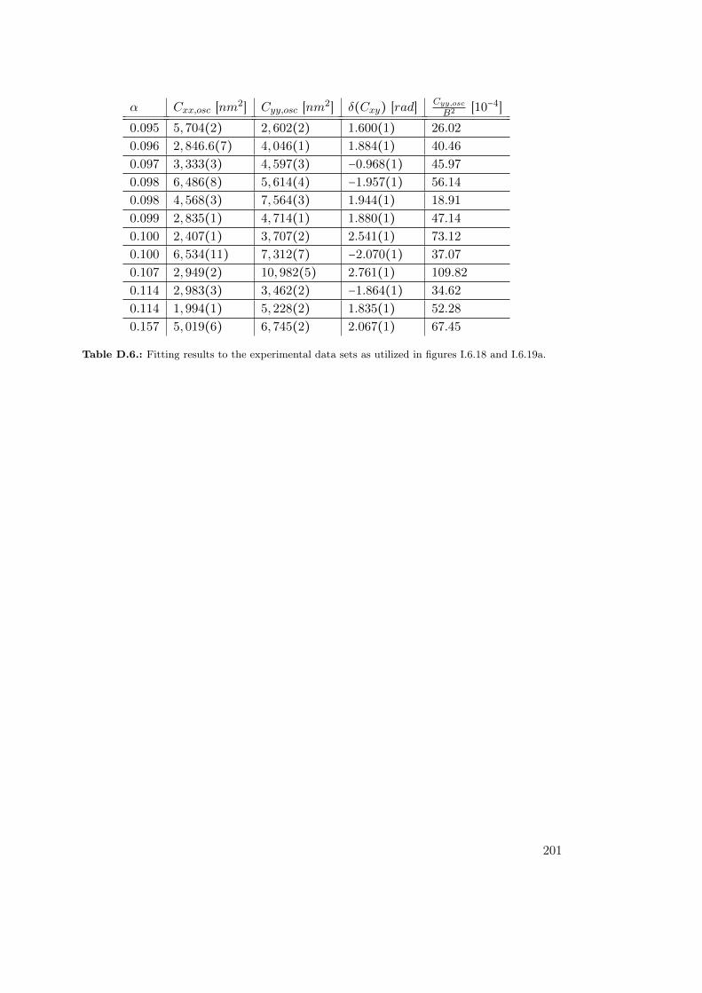
α Cxx,osc [nm2] Cyy,osc [nm2] δ(Cxy) [rad] Cyy,osc
B2 [10−4]
0.095 5,704(2) 2,602(2) 1.600(1) 26.02
0.096 2,846.6(7) 4,046(1) 1.884(1) 40.46
0.097 3,333(3) 4,597(3) −0.968(1) 45.97
0.098 6,486(8) 5,614(4) −1.957(1) 56.14
0.098 4,568(3) 7,564(3) 1.944(1) 18.91
0.099 2,835(1) 4,714(1) 1.880(1) 47.14
0.100 2,407(1) 3,707(2) 2.541(1) 73.12
0.100 6,534(11) 7,312(7) −2.070(1) 37.07
0.107 2,949(2) 10,982(5) 2.761(1) 109.82
0.114 2,983(3) 3,462(2) −1.864(1) 34.62
0.114 1,994(1) 5,228(2) 1.835(1) 52.28
0.157 5,019(6) 6,745(2) 2.067(1) 67.45
Table D.6.: Fitting results to the experimental data sets as utilized in figures I.6.18 and I.6.19a.
201

D. Supplementary Tables
α δ(Cxy) [rad]0.015 −1.4(4)0.024 −1.2(4)0.032 −1.5(−)0.054 −0.3(7)0.064 −1.35(3)0.074 −1(1)0.084 −1.19(1)0.096 −1.4(3)0.103 −1.0(9)0.114 −1.6(4)0.157 −1.1(−)
Table D.7.: Phase shifts of the cross-correlation function Cxy after removal of the influence of the signof the shear gradient and after averaging of the data within frequency intervals of a width∆α = 0.01. These data sets were also plotted in figure I.6.19. No errors are given forα = 0.032 and α = 0.157 since only one single value was contained in the correspondingaveraging interval.
202

f [Hz] G′1 [Pa] G′′
1 [Pa] δ1 [rad] G′2 [Pa] G′′
2 [Pa] δ2 [rad]1 ⋅ 10−2 3,921 692 10.01 2,863 602 11.88
2 ⋅ 10−2 4,715 917 11.01 3,414 757 12.50
3 ⋅ 10−2 5,337 1028 10.91 3,812 788 11.69
4 ⋅ 10−2 5,513 1015 10.44 4,152 718 9.81
5 ⋅ 10−2 5,874 887 8.59 4,343 663 8.68
6 ⋅ 10−2 6,309 802 7.25 4,420 667 8.59
7 ⋅ 10−2 6,052 965 9.06 4,557 784 9.76
8 ⋅ 10−2 5,986 915 8.69 4,684 723 8.77
9 ⋅ 10−2 5,946 845 8.09 4,753 691 8.27
1 ⋅ 10−1 6,186 774 7.14 4,873 627 7.33
2 ⋅ 10−1 6,777 763 6.42 5,169 627 6.92
3 ⋅ 10−1 6,865 862 7.16 5,433 714 7.48
4 ⋅ 10−1 6,770 826 6.96 5,457 669 6.99
5 ⋅ 10−1 7,219 692 5.47 5,628 586 5.94
6 ⋅ 10−1 6,900 832 6.87 5,676 679 6.82
7 ⋅ 10−1 7,118 789 6.32 5,593 661 6.74
8 ⋅ 10−1 7,062 844 6.82 5,536 660 6.80
9 ⋅ 10−1 7,688 781 5.80 5,820 581 5.70
1 ⋅ 100 8,076 926 6.54 5,987 705 6.72
2 ⋅ 100 8,716 1,094 7.15 6,271 793 7.20
3 ⋅ 100 8,704 1,208 7.90 6,310 878 7.93
4 ⋅ 100 9,076 1,390 8.71 6,497 978 8.56
5 ⋅ 100 9,237 1,520 9.35 6,542 1056 9.17
6 ⋅ 100 9,053 1,121 7.06 6,322 751 6.77
7 ⋅ 100 9,207 1,161 7.19 6,374 781 6.99
8 ⋅ 100 9,340 1,205 7.35 6,473 805 7.09
9 ⋅ 100 9,425 1,225 7.40 6,457 826 7.29
1 ⋅ 101 9,502 1,270 7.61 6,422 866 7.68
Table D.8.: Results from macrorheological SAOS results as plotted in figure II.4.5. Data recorded atthe mucus sample from the first horse carries the index 1, data from the second horse isindicated by the index 2.
203


Acknowledgements
First and foremost, I would like to thank Prof. Dr. Christian Wagner for giving me theopportunity to work on topics like cross-correlations of Brownian motion and complexfluids in his group. Also, I would like to thank him for the chance to work on the DNAproject in Strasbourg.
I would like to thank Prof. Dr. Carlos Marques for his support when planning the DNAproject and for his supervision during its course. Many fruitful discussions together withAndré Schröder, Pierre Muller, and Tatiana Schmatko brought fresh ideas and helped inthe advancement of the experiments.
Many thanks go to the complete Wagner and Huber groups in Saarbrücken as well as theMarques group in Strasbourg for their great atmosphere and colleagueship. Wheneverchemical mixtures were necessary, Karin Kretsch was there to advise and help out, ifthere was any bureaucratical issue, Elke Huschens knew the answer. Thus, additionalthanks are reserved for them.
A further thank you goes to the mechanical as well as the electronics workshop of theexperimental physics department in Saarbrücken.
I would like to thank Devin Townsend and many more excellent heavy metal bands forthe best soundtrack to a dissertation. Also, big thanks go to the many indie game devel-opers out there for really great games like “Papers, please!”, “The Stanley Parable”, andall the others which helped in gaining the necessary distance from my own work.
I would also like to thank my two proofreaders, Elke and Dominik, for their patience inhunting spelling and other errors as well as the mapping of labyrinthine sentences.
An immensely big thank you goes to my parents and my whole family. Without theirsupport while growing up and during my studies later I would never have come this far!
The biggest acknowledgement goes to my fiancée Elke. Thank you for always bearingwith me, especially during hard times, and for always supporting me! I couldn’t havedone this without you!
205


Eidesstattliche Versicherung
Hiermit versichere ich an Eides statt, dass ich die vorliegende Arbeit selbstständig undohne Benutzung anderer als der angegebenen Hilfsmittel angefertigt habe. Die aus an-deren Quellen oder indirekt übernommenen Daten und Konzepte sind unter Angabe derQuelle gekennzeichnet.
Die Arbeit wurde bisher weder im In- noch im Ausland in gleicher oder ähnlicher Formin einem Verfahren zur Erlangung eines akademischen Grades vorgelegt.
Saarbrücken, 10. September 2014
Andreas Gross
207


List of Variables
symbol unit meaning
ACij m2 amplitude of non-oscillating contribution to cross-correlation func-tion Cij
ADNA m amplitude of DNA center of massArel m relative amplitude of DNA center of mass in respect to driving lensAresc m rescaled amplitude of DNA center of mass in respect to driving
lens amplitude and relative heightB m amplitude of driving oscillationc m
s speed of light in vacuumCii m2 auto-correlation function of direction iCij m2 cross-correlation function of direction i and direction jCij,osc m2 amplitude of oscillating contribution to cross-correlation functiondc m diameter of colloiddcw m distance of wall and center of a colloidD m2
s diffusion coefficientE A2 s4
kgm3 electric fieldf 1
s frequencyFgrad
kgms2
gradient forceFr
kgms2
Brownian random forceFscat
kgms2
scattering forceFtrap
kgms2
restoring force of the optical trapg m
s2gravitational acceleration
G, G kgms2
shear modulusG′ kg
ms2elastic contribution to shear modulus
G′′ kgms2
viscous contribution to shear modulushlens m distance between coverslide and lenskB
kgm2
s2KBoltzmann’s constant
k, ktrap kgs2
trap stiffnessm kg massmr − relative refractive index
This table continues on the following page.
209

D. Supplementary Tables
symbol unit meaning
nc − refractive index of colloid materialnm − refractive index of surrounding mediump kg
ms2pressure
P kgm2
s3power of a laser beam
Q m3
s flow rateQgrad − quality factor of gradient forceQscat − quality factor of scattering forcerc m radius of colloidRe − Reynolds numberRF − Fresnel’s coefficient of reflectionrtrap m position vector of trapS kg
s3Poynting vector
T K temperatureTF − Fresnel’s coefficient of transmissionWi − Weissenberg numberz0 m average distance of grafted DNA center of mass from coverslideα − dimensionless frequencyα s2
kg fluid susceptibilityαp
A2s4
kg electromagnetic polarizabilityγ − shear strainγ 1
s shear rateδ rad phaseδDNA rad phase of DNA center of massδlens rad phase of lensζ kg
s coefficient of frictionη kg
ms dynamic viscosityθi rad angle of incidenceθe rad angle of emergenceκ kg
s2spring constant
λ m wavelengthρ kg
m3 densityσs m2 scattering cross-sectionτ kg
ms2shear stress
τr1s relaxation rate
ω rads angular frequency
210

List of Figures
I.1.1. Arbitrary path of a colloidal particle in the bulk of a fluid . . . . . . . 7
I.2.1. Contributions of correlated and anti-correlated modes of motion of twobeads along the same coordinate axis . . . . . . . . . . . . . . . . . . . 10
I.3.1. Quality factors for scattering (Eq. I.3.6) and gradient force (Eq. I.3.7) 15I.3.2. Total force balance of scattering and gradient force for the interaction
of a focused laser beam with a sphere . . . . . . . . . . . . . . . . . . . 17
I.4.1. Color-coded plot of the flow velocity in the x-direction of a rectangularchannel in the y-z-plane . . . . . . . . . . . . . . . . . . . . . . . . . . . 20
I.4.2. Plot of the normalized flow velocity v against the position y . . . . . . 21I.4.3. Mask used for lithographic processing of the mold . . . . . . . . . . . . 23I.4.4. Photograph of a fully prepared microfluidic device . . . . . . . . . . . . 24I.4.5. Sketch of a colloid in a microfluidic device with a rectangular cross-
section . . . . . . . . . . . . . . . . . . . . . . . . . . . . . . . . . . . . . . 26I.4.6. Analytical auto-correlation functions of a colloid confined in an optical
trap . . . . . . . . . . . . . . . . . . . . . . . . . . . . . . . . . . . . . . . 29I.4.7. Analytical cross-correlation functions of a colloid confined in an optical
trap . . . . . . . . . . . . . . . . . . . . . . . . . . . . . . . . . . . . . . . 30I.4.8. Sketch of a colloid which is driven to oscillations in y-direction in a
microfluidic device with a rectangular cross-section . . . . . . . . . . . 32I.4.9. Analytical auto-correlation functions of a colloid forced by an oscillat-
ing optical trap . . . . . . . . . . . . . . . . . . . . . . . . . . . . . . . . . 35I.4.10. Analytical cross-correlation functions of a colloid forced by an oscil-
lating optical trap . . . . . . . . . . . . . . . . . . . . . . . . . . . . . . . 35I.4.11. Dependence of the phase of the cross-correlation function Cxy on α . 36
I.5.1. Histogram of displacements of a numerical data set of a colloid in anoptical trap . . . . . . . . . . . . . . . . . . . . . . . . . . . . . . . . . . . 40
I.5.2. Auto- and cross-correlation functions of a simulated displacement of acolloid out of the center of an optical trap . . . . . . . . . . . . . . . . . 41
I.5.3. Cross-correlation function of a numerical dataset of the displacementof a colloid out of the center of an optical trap in a linear shear flow . 42
211

List of Figures
I.5.4. Correlation functions Cxx, Cyy, and Cxy for a colloid in linear shearflow forced by an oscillating optical trap . . . . . . . . . . . . . . . . . . 44
I.5.5. Dependence of the oscillation amplitudes of the auto- and cross-correlationfunctions on the shear rate . . . . . . . . . . . . . . . . . . . . . . . . . . 45
I.5.6. Dependence of the relative correlation amplitude Cxx,osc/Cyy,osc on theoscillation frequency of the optical trap . . . . . . . . . . . . . . . . . . 46
I.5.7. Phase behavior of Cxy as a function of the dimensionless frequency ata fixed relaxation rate τr . . . . . . . . . . . . . . . . . . . . . . . . . . . 48
I.6.1. Illustration of the setup of optical tweezers . . . . . . . . . . . . . . . . 53I.6.2. Power of each of the laser beams measured by a power meter . . . . . 54I.6.3. Beam profiles of the two lasers utilized in the setup of optical tweezers 55I.6.4. Characteristic transmission line for both of the dichroic mirrors utilized
in the setup of optical tweezers. . . . . . . . . . . . . . . . . . . . . . . . 56I.6.5. Characteristic transmission line for the two rejection band filters uti-
lized in the setup of optical tweezers. . . . . . . . . . . . . . . . . . . . . 58I.6.6. Influence of the camera angle alignment on the correlation functions
of the displacements of a trapped bead . . . . . . . . . . . . . . . . . . 63I.6.7. Typical displacement curve recorded for the tilt calibration of the camera 64I.6.8. Results of multiple independent drag force calibrations with sinewave
oscillations at different laser emission power settings . . . . . . . . . . 69I.6.9. Trap stiffnesses resulting from different calibration methods . . . . . . 69I.6.10. Auto- and Cross-correlation functions with no flow present. . . . . . . 70I.6.11. Auto- and cross-correlation functions of two independent measure-
ments M1 and M2 at the same experimental settings . . . . . . . . . . 72I.6.12. Influence of the sign of the shear gradient in a linear shear flow . . . . 73I.6.13. Dependence of the depth and position of the cross-correlation peak
near t = 0 s on the trap stiffness . . . . . . . . . . . . . . . . . . . . . . . 74I.6.14. Effect of the sign of the shear gradient on the confinement of a colloid 76I.6.15. Effect of the sign of the shear gradient on the spatial distribution of a
colloid . . . . . . . . . . . . . . . . . . . . . . . . . . . . . . . . . . . . . . 77I.6.16. Auto-correlation functions Cxx and Cyy for a colloid confined in an
oscillating trap (k = 5.5µN/m) in a linear shear flow about 3rc awayfrom the channel walls . . . . . . . . . . . . . . . . . . . . . . . . . . . . 79
I.6.17. Cross-correlation functions Cxy for a colloid confined in an oscillatingtrap (k = 5.5µN/m) in a linear shear flow about 3rc away from thechannel walls . . . . . . . . . . . . . . . . . . . . . . . . . . . . . . . . . . 80
I.6.18. Dependence of the oscillatory contribution to the auto-correlation func-tion Cyy on the dimensionless frequency α . . . . . . . . . . . . . . . . 82
212

List of Figures
I.6.19. Phase behavior of the oscillatory contribution to Cxy . . . . . . . . . . 82
II.1.1. Scanning-electron-micrograph of the cilia found in the rabbit trachea 97
II.2.1. Cryo-scanning-electron micrograph of respiratory horse mucus . . . . 100
II.3.1. Equivalent circuit diagram of the Maxwell model . . . . . . . . . . . . 102II.3.2. Typical curve progression of the shear modulus according to Maxwell’s
model . . . . . . . . . . . . . . . . . . . . . . . . . . . . . . . . . . . . . . 103
II.4.1. Photograph of the utilized rheometer HAAKE MARS II as well as allof its crucial components. . . . . . . . . . . . . . . . . . . . . . . . . . . 111
II.4.2. Evaluation of the linear response range via an amplitude sweep witha mucus sample . . . . . . . . . . . . . . . . . . . . . . . . . . . . . . . . 114
II.4.3. Lissajous-figures gained by an amplitude sweep with a mucus sample 115II.4.4. Lissajous-figures gained by an amplitude sweep with a polyacrylamide
(PAAm) sample . . . . . . . . . . . . . . . . . . . . . . . . . . . . . . . . 115II.4.5. Results from small amplitude oscillatory shear experiments performed
at two mucus samples stemming from two different horses . . . . . . . 116II.4.6. Mean squared displacements from passive tracking experiments at dif-
ferent positions within the same mucus sample . . . . . . . . . . . . . . 121II.4.7. Overview of the distribution of mean squared displacements within a
1 % hydroethoxycellulose (HEC) sample. The x- and y-component ateach position is plotted independently (marked by different symbolsof the same color). This graph was adapted from figure 4B in [76]. . . 122
II.4.8. Results from passive particle tracking experiments at different posi-tions within the same mucus sample . . . . . . . . . . . . . . . . . . . . 123
II.4.9. Oscillatory displacement experiments at two different positions withinthe same mucus sample . . . . . . . . . . . . . . . . . . . . . . . . . . . . 126
II.5.1. Comparison of the shear modulus recovered from macrorheologic SAOSexperiments with the results from passive microrheology . . . . . . . . 130
II.5.2. Sketch of the microscopic structure of mucus . . . . . . . . . . . . . . . 131
III.3.1. Planar structural binding model of a DNA molecule . . . . . . . . . . . 145III.3.2. Sketch of the oscillating, linear flow profile between a fixed lower plate
and an oscillating upper plate . . . . . . . . . . . . . . . . . . . . . . . . 148III.3.3. Dependence of the velocity amplitude and the phase shift of the moving
fluid on the position in z-direction between the plates . . . . . . . . . . 149III.3.4. Model system for single-end-grafted DNA molecules on a cover slip. . 150III.3.5. Results of the bead-spring model for DNA molecules . . . . . . . . . . 153
213

List of Figures
III.4.1. Ligation process of λ-DNA in preparation for single-end-grafting . . . 156III.4.2. Representation of the experimental setup for shearing and visualizing
the DNA molecules . . . . . . . . . . . . . . . . . . . . . . . . . . . . . . 158III.4.3. Calibration curve of lens amplitude versus piezo voltage . . . . . . . . 160III.4.4. Comparison of originally recorded picture of grafted DNA molecules
and post-processed picture after filtering . . . . . . . . . . . . . . . . . 161III.4.5. Displacement-time-diagram of the lens and the center-of-mass of a
DNA molecule as well as sinusoidal fits to both data sets . . . . . . . . 163III.4.6. Auto-correlation functions of the motion of a DNA molecule under
sinusoidal driving . . . . . . . . . . . . . . . . . . . . . . . . . . . . . . . 164III.4.7. Histogram of the longest relaxation rates of the DNA molecules . . . 164III.4.8. Graph of the DNA COM versus the lens amplitude . . . . . . . . . . . 165III.4.9. Dependencies of the relative amplitude and the phase shift on the
distance between oscillation lens and cover slip . . . . . . . . . . . . . . 166III.4.10. Amplitude dependency on the dimensionless frequency . . . . . . . . . 167III.4.11. Dependency of the phase shift between driving and response oscillation
on the dimensionless frequency . . . . . . . . . . . . . . . . . . . . . . . 168III.4.12. Plot of the results of the length evaluation of the DNA intensity profile
versus the evaluation using sine fits to the COM motion . . . . . . . . 170III.4.13. Plot of the results of the length evaluation of the DNA intensity profile
as compared to the width of the equilibrium intensity distribution ofsuch a molecule . . . . . . . . . . . . . . . . . . . . . . . . . . . . . . . . 170
III.5.1. Results of the experimental study of M. Khaksar with single-end-grafted DNA . . . . . . . . . . . . . . . . . . . . . . . . . . . . . . . . . . 175
214

List of Tables
A.1. Chemical products and microparticles utilized to conduct the experimentsin all parts of this thesis. . . . . . . . . . . . . . . . . . . . . . . . . . . . . . 185
D.1. Data sets shown in figures I.5.5b. . . . . . . . . . . . . . . . . . . . . . . . . 197D.2. Data sets shown in figures I.5.6 and I.5.7. . . . . . . . . . . . . . . . . . . . 197D.3. Data set of the emitted laser power of the Ventus laser utilized in the setup
of optical tweezers in Saarbrücken . . . . . . . . . . . . . . . . . . . . . . . . 198D.4. Data set of the emitted laser power of the Ciel laser utilized in the setup
of optical tweezers in Saarbrücken . . . . . . . . . . . . . . . . . . . . . . . . 199D.5. Results of all calibration methods detailed in section I.6.3 . . . . . . . . . 199D.6. Fitting results to the experimental data sets . . . . . . . . . . . . . . . . . . 201D.7. Phase shifts of the cross-correlation function Cxy after removal of the in-
fluence of the sign of the shear gradient and after averaging of the datawithin frequency intervals of a width ∆α = 0.01. These data sets were alsoplotted in figure I.6.19. No errors are given for α = 0.032 and α = 0.157
since only one single value was contained in the corresponding averaginginterval. . . . . . . . . . . . . . . . . . . . . . . . . . . . . . . . . . . . . . . . 202
D.8. Macrorheological SAOS results . . . . . . . . . . . . . . . . . . . . . . . . . . 203
215


Bibliography
[1] Anderson, V. J. and Lekkerkerker, H. N. W.; “Insight into Phase Transition Kinetics fromColloid Science”; Nature 416 (2002) 811
[2] Radu, M. and Schilling, T.; “Hydrodynamic Interactions of Colloidal Spheres under ShearFlow”; arXiv cond-mat.soft:1203 (2012) 1203.3441v1
[3] Ashkin, A., Dziedzic, J. M., Bjorkholm, J. E., and Chu, S.; “Observation of a Single-BeamGradient Force Optical Trap for Dielectric Particles”; Optics Letters 11 (1986) 288
[4] Ziehl, A.; Untersuchung Brownscher Partikel im Scherfluss durch Korrelationsanalysenunter Verwendung optischer Pinzetten; Ph.D. thesis; Universität des Saarlandes (2009)
[5] Ziehl, A., Bammert, J., Holzer, L., Wagner, C., and Zimmermann, W.; “Direct Measure-ment of Shear-Induced Cross-Correlation of Brownian Motion”; Physical Review Letters103 (2009) 230602
[6] Ingenhousz, J. and Molitor, N. C.; Vermischte Schriften physisch-medicinischen Inhalts;Wappler (1784)
[7] Brown, R.; “A Brief Account of Microscopic Observation Made in the Months of June, July,and August, 1827, on the Particles Contained in the Pollen of Plants and on the GeneralExistence of Active Molecules in Organic and Inorganic Bodies”; Philosophical Magazine4 (1828) 161
[8] Wiener, C.; “Erklärung des atomistischen Wesens des tropfbar-flüssigen Körperzustandes,und Bestätigung desselben durch die sogenannten Molecularbewegungen”; Annalen derPhysik und Chemie 194 (1863) 79
[9] Exner, S.; “Untersuchung über Brown’s molecularbewegung”; Sitzungsberichte der Kaiser-lichen Academie der Wissenschaften 56 (1867) 116
[10] Delsaulx, J.; “Thermo-dynamic Origin of the Brownian Motions”; The Monthly Microsco-pical Journal 18 (1877) 1
[11] Einstein, A.; “Über die von der molekularkinetischen Theorie der Wärme geforderte Be-wegung von in ruhenden Flüssigkeiten suspendierten Teilchen”; Annalen der Physik 322(1905) 549
[12] Smoluchowski, M.; “Zur kinetischen Theorie der Brownschen Molekularbewegung und derSuspensionen”; Annalen der Physik 326 (1906) 756
[13] Perrin, J. and Dabrowski, M.; “Mouvement Brownien et Constantes Moléculaires”;Comptes Rendus de l’Académie des Sciences de Paris 149 (1909) 477
[14] Maret, G. and Wolf, P. E.; “Multiple Light Scattering from Disordered Media. The Effectof Brownian Motion of Scatterers”; Zeitschrift fuer Physik B - Condensed Matter 65 (1987)409
217

Bibliography
[15] Ehrenberg, M. and Rigler, R.; “Rotational Brownian Motion and Fluorescence IntensityFluctuations”; Chemical Physics 4 (1974) 390
[16] Meiners, J.-C. and Quake, S. R.; “Direct Measurement of Hydrodynamic Cross Correlationsbetween Two Particles in an External Potential”; Physical Review Letters 82 (1999) 2211
[17] Skryabina, M. N., Lyubin, E. V., Khokhlova, M. D., and Fedyanin, A. A.; “Probing of PairInteraction of Magnetic Microparticles with Optical Tweezers”; JETP Letters 95 (2012)560
[18] Bammert, J., Holzer, L., and Zimmermann, W.; “Dynamics of Two Trapped BrownianParticles: Shear-Induced Cross-Correlations”; European Physical Journal E: Soft Matter33 (2010) 313
[19] Holzer, L., Bammert, J., Rzehak, R., and Zimmermann, W.; “Dynamics of a TrappedBrownian Particle in Shear Flows”; Physical Review E 81 (2010) 041124
[20] Santiago, J. G., Wereley, S. T., Meinhart, C. D., Beebe, D. J., and Adrian, R. J.; “AParticle Image Velocimetry System for Microfluidics”; Experiments in Fluids 25 (1998)316
[21] Meinhart, C. D., Wereley, S. T., and Santiago, J. G.; “PIV Measurements of a MicrochannelFlow”; Experiments in Fluids (1999)
[22] Olsen, M. G. and Adrian, R. J.; “Brownian Motion and Correlation in Particle ImageVelocimetry”; Optics & Laser Technology 32 (2000) 621
[23] Hohreiter, V., Wereley, S. T., Olsen, M. G., and Chung, J. N.; “Cross-Correlation Analysisfor Temperature Measurement”; Measurement Science and Technology (2002)
[24] Volpe, G. and Petrov, D.; “Torque Detection Using Brownian Fluctuations”; PhysicalReview Letters 97 (2006) 210603
[25] Einstein, A.; “Über einen die Erzeugung und Verwandlung des Lichtes Betreffenden Heuris-tischen Gesichtspunkt”; Annalen der Physik 14 (1905) 164
[26] Ashkin, A.; “Acceleration and Trapping of Particles by Radiation Pressure”; Physical Re-view Letters 24 (1970) 156
[27] Ashkin, A. and Dziedzic, J. M.; “Optical Levitation by Radiation Pressure”; AppliedPhysics Letters 19 (1971) 283
[28] Ashkin, A.; “Trapping of Atoms by Resonance Radiation Pressure”; Physical Review Let-ters 40 (1978) 729
[29] Gordon, J. P. and Ashkin, A.; “Motion of Atoms in a Radiation Trap”; Physical Review A21 (1980) 1606
[30] Ashkin, A.; “Forces of a Single-Beam Gradient Laser Trap on a Dielectric Sphere in theRay Optics Regime”; Biophysical Journal 61 (1992) 569
[31] Simmons, R. M., Finer, J. T., Warrick, H. M., Kralik, B., Chu, S., and Spudich, J. A.;“Force on Single Actin Filaments in a Motility Assay Measured with an Optical Trap”;Advances in Experimental Medicine and Biology 332 (1993) 331
[32] Khan, S. and Sheetz, M. P.; “Force Effects on Biochemical Kinetics”; Annual Review ofBiochemistry 66 (1997) 785
[33] Mehta, A. D., Finer, J. T., and Spudich, J. A.; “Use of Optical Traps in Single-Molecule
218

Bibliography
Study of Nonprocessive Biological Motors”; Methods in Enzymology 298 (1998) 436[34] Perkins, T. T., Quake, S. R., Smith, D. E., and Chu, S.; “Relaxation of a Single DNA
Molecule Observed by Optical Microscopy”; Science 264 (1994) 822[35] Wang, M. D., Yin, H., Landick, R., Gelles, J., and Block, S. M.; “Stretching DNA with
Optical Tweezers”; Biophysical Journal 72 (1997) 1335[36] Mason, T. G. and Weitz, D. A.; “Optical Measurements of Frequency-Dependent Linear
Viscoelastic Moduli of Complex Fluids”; Physical Review Letters 74 (1995) 1250[37] Valentine, M. T., Dewalt, L. E., and Ou-Yang, H. D.; “Forces on a Colloidal Particle in
a Polymer Solution: a Study Using Optical Tweezers”; Journal of Physics: CondensedMatter 8 (1996) 9477
[38] van Zanten, J. H., Amin, S., and Abdala, A. A.; “Brownian Motion of Colloidal Spheresin Aqueous PEO Solutions”; Macromolecules 37 (2004) 3874
[39] Valentine, M. T., Kaplan, P. D., Thota, D., Crocker, J. C., Gisler, T., Prud’homme, R. K.,Beck, M., and Weitz, D. A.; “Investigating the Microenvironments of Inhomogenous SoftMaterials with Multiple Particle Tracking”; Physical Review E 64 (2001) 061506
[40] Williams, M. A. K., Vincent, R. R., Pinder, D. N., and Hemar, Y.; “MicrorheologicalStudies offer Insights into Polysaccharide Gels”; Journal of Non-Newtonian Fluid Mechanics49 (2008) 63
[41] Addas, K. M., Schmidt, C. F., and Tang, J. X.; “Microrheology of Solutions of SemiflexibleBiopolymer Filaments Using Laser Tweezers Interferometry”; Physical Review E 70 (2004)021503
[42] Brau, R. R., Ferrer, J. M., Lee, H., Castro, C. E., Tam, B. K., Tarsa, P. B., Matsudaira,P., Boyce, M. C., Kamm, R. D., and Lang, M. J.; “Passive and Active Microrheology withOptical Tweezers”; Journal of Optics A: Pure and Applied Optics 9 (2007) S103
[43] Weihs, D., Mason, T. G., and Teitell, M. A.; “Bio-Microrheology: A Frontier in Microrhe-ology”; Biophysical Journal 91 (2006) 4296
[44] Bohren, C. F. and Huffman, D. R.; Absorption and Scattering of Light by Small Particles;Wiley-VCH; 1st edition (2004)
[45] Chaumet, P. C. and Nieto-Vesperinas, M.; “Coupled Dipole Method Determination of theElectromagnetic Force on a Particle over a Flat Dielectric Substrate”; Physical Review B61 (2000) 14119
[46] Maheu, B., Gouesbet, G., and Grehan, G.; “A Concise Presentation of the GeneralizedLorenz-Mie Theory for Arbitrary Location of the Scatterer in an Arbitrary Incident Profile”;Journal of Optics 19 (1988) 59
[47] Ren, K. F., Grehan, G., and Gouesbet, G.; “Prediction of Reverse Radiation Pressure byGeneralized Lorenz-Mie Theory”; Applied Optics 35 (1996) 2702
[48] Wohland, T., Rosin, A., and Stelzer, E. H. K.; “Theoretical Determination of the Influenceof the Polarization on Forces Exerted by Optical Tweezers”; Optik 102 (1996) 181
[49] Bird, R. B., Armstrong, R. C., and Hassager, O.; Dynamics of Polymeric Liquids: Volume1 Fluid Mechanics; volume 1; Wiley-Interscience (1987)
[50] Pozrikidis, C.; Introduction to Theoretical and Computational Fluid Dynamics; Oxford
219

Bibliography
University Press (1997)[51] Happel, J. and Brenner, H.; Low Reynolds Number Hydrodynamics with Special Applica-
tions to Particulate Media; Springer Verlag; 2nd edition (2009)[52] Xia, Y. and Whitesides, G. M.; “Soft Lithography”; Angewandte Chemie, International
Edition 37 (1998) 550[53] Huang, R., Chavez, I., Taute, K. M., Lukic, B., Jeney, S., Raizen, M. G., and Florin, E.-L.;
“Direct Observation of the Full Transition from Ballistic to Diffusive Brownian Motion ina Liquid”; Nature Physics 7 (2011) 576
[54] Uhlenbeck, G. E. and Ornstein, L. S.; “On the Theory of the Brownian Motion”; PhysicalReview 36 (1930) 823
[55] Callen, H. B. and Welton, T. A.; “Irreversibility and Generalized Noise”; Physical Review83 (1951) 34
[56] Mason, T. G., Gang, H., and Weitz, D. A.; “Rheology of Complex Fluids Measured byDynamic Light Scattering”; Journal of Molecular Structure 383 (1996) 81
[57] Langevin, P.; “Sur la Théorie du Mouvement Brownien”; Comptes Rendus de l’Académiedes Sciences (Paris) 146 (1908) 530
[58] Chakraborty, D.; “Time Correlations and Persistence Probability of a Brownian Particlein a Shear Flow”; European Physical Journal B: Condensed Matter Physics 85 (2012) 281
[59] Zeidler, E.; Springer-Taschenbuch der Mathematik; Springer Spektrum (2013)[60] Protter, P. E.; Stochastic Integration and Differential Equations; Springer Berlin Heidel-
berg; 2nd edition (2005)[61] Neuman, K. C. and Block, S. M.; “Optical Trapping”; Review of Scientific Instruments 75
(2004) 2787[62] Schwabl, F.; Statistische Mechanik; chapter Brownsche Bewegung, Stochastische Bewe-
gungsgleichungen und Fokker-Planck-Gleichungen, 417–444; Springer Berlin Heidelberg;3rd edition (2006)
[63] Fällman, E. and Axner, O.; “Influence of a Glass-Water Interface on the On-Axis Trappingof Micrometer-Sized Spherical Objects by Optical Tweezers”; Applied Optics 42 (2003)3915
[64] Jung, A.; Untersuchung einer Ca2+-induzierten Erythrozytenadhäsion mittels holo-graphischer optischer Pinzetten; Ph.D. thesis; Universität des Saarlandes (2008)
[65] Capitanio, M., Romano, G., Ballerini, R., Giuntini, M., Pavone, F. S., Dunlap, D., andFinzi, L.; “Calibration of Optical Tweezers with Differential Interference Contrast Signals”;Review of Scientific Instruments 73 (2002) 1687
[66] Peterman, E. J. G., Gittes, F., and Schmidt, C. F.; “Laser-Induced Heating in OpticalTraps”; Biophysical Journal 84 (2003) 1308
[67] Fischer, M. and Berg-Sørensen, K.; “Calibration of Trapping Force and Response Functionof Optical Tweezers in Viscoelastic Media”; Journal of Optics A: Pure and Applied Optics9 (2007) S239
[68] Werth, M.; Verhalten komplexer Fluide am Stagnationspunkt einer Elongationsströmung;Diploma thesis; Universität des Saarlandes (2012)
220

Bibliography
[69] Dekker, J., Rossen, J. W. A., Büller, H. A., and Einerhand, A. W. C.; “The MUC Family:an Obituary”; Trends in Biochemical Sciences 27 (2002) 126
[70] Bansil, R. and Turner, B. S.; “Mucin Structure, Aggregation, Physiological Functions andBiomedical Applications”; Current Opinion in Colloid & Interface Science 11 (2006) 164
[71] Lai, S. K., Wang, Y.-Y., Wirtz, D., and Hanes, J.; “Micro- and Macrorheology of Mucus”;Advanced Drug Delivery Reviews 61 (2009) 86
[72] Olmsted, S. S., Padgett, J. L., Yudin, A. I., Whaley, K. J., Moench, T. R., and Cone,R. A.; “Diffusion of Macromolecules and Virus-Like Particles in Human Cervical Mucus”;Biophysical Journal 81 (2001) 1930
[73] Cone, R. A.; “Barrier Properties of Mucus”; Advanced Drug Delivery Reviews 61 (2009)75
[74] Sanderson, M. J. and Sleigh, M. A.; “Ciliary Activity of Cultured Rabbit Tracheal Epithe-lium: Beat Pattern and Metachrony”; J. Cell Sci. 47 (1981) 331
[75] Sigurdsson, H. H., Kirch, J., and Lehr, C.-M.; “Mucus as a Barrier to Lipophilic Drugs”;International Journal of Pharmaceutics 453 (2013) 56
[76] Kirch, J., Schneider, A., Abou, B., Hopf, A., Schäfer, U. F., Schneider, M., Schall, C., Wag-ner, C., and Lehr, C.-M.; “Optical Tweezers Reveal Relationship between Microstructureand Nanoparticle Penetration of Pulmonary Mucus”; Proceedings of the National Academyof Sciences of the United States of America 109 (2012) 18355
[77] Denton, R.; “Rheology of Human Lung Mucus”; Annals of the New York Academy ofSciences 106 (1963) 746
[78] Odeblad, E.; “The Functional Structure of Human Cervical Mucus”; Acta Obstetricia etGynecologica Scandinavica 47 (1968) 57
[79] Denton, R., Forsman, W., Hwang, S. H., Litt, M., and Miller, C. E.; “Viscoelasticityof Mucus - Its Role in Ciliary Transport of Pulmonary Secretions”; American Review ofRespiratory Disease 98 (1968) 380
[80] Litt, M.; “Mucus Rheology - Relevance to Muciliary Clearance”; Archives of InternalMedicine 126 (1970) 417
[81] Eliezer, N.; “Viscoelastic Properties of Mucus”; Biorheology 11 (1974) 61[82] Button, B., Cai, L.-H., Ehre, C., Kesimer, C., Hill, D. B., Sheehan, J. K., Boucher, R. C.,
and Rubinstein, M.; “A Periciliary Brush Promotes the Lung Health by Separating theMucus Layer from Airway Epithelia”; Science 337 (2012) 937
[83] Mason, T. G., Ganesan, K., van Zanten, J. H., Wirtz, D., and Kuo, S. C.; “ParticleTracking Microrheology of Complex Fluids”; Physical Review Letters 79 (1997) 3282
[84] Lai, S. K., O’Hanlon, D. E., Harrold, S., Man, S. T., Wang, Y.-Y., and Cone, R.; “RapidTransport of Large Polymeric Nanoparticles in Fresh Undiluted Human Mucus”; Proceed-ings of the National Academy of Sciences of the United States of America 104 (2007)1482
[85] Doraiswamy, D.; “The Origins of Rheology: a Short Historical Excursion”; RheologyBulletin 71 (2002); URL http://www.rheology.org/SoR/publications/Rheology%5FB/Jan02/Origin_of_Rheology.pdf
221

Bibliography
[86] Maxwell, J. C.; “On the Dynamical Theory of Gases”; Philosophical Transactions of theRoyal Society of London 157 (1867) 49
[87] Mooney, M. and Ewart, R. H.; “The Conicylindrical Viscometer”; R. H. Physics 5 (1934)350
[88] Russell, R. J.; The Determination of the Basic Rheological Constants Governing the Flowof Pseudoplastic Substances; Ph.D. thesis; University of London (1946)
[89] Gill, F. and Russell, R. J.; “Pumpability of Residual Fuel Oils”; Industrial & EngineeringChemistry Research 46 (1954) 1264
[90] Philippoff, W. and Gaskins, F. H.; “Viscosity Measurements on Molten Polyethylene”;Journal of Polymer Science, Part A: Polymer Chemistry 21 (1956) 205
[91] Higginbotham, R. S.; “A Cone and Plate Viscometer”; Journal of Scientific Instruments 27(1950) 139
[92] McKennell, R.; “Cone-Plate Viscometer”; Analytical Chemistry 28 (1956) 1710[93] Walters, K. and Kemp, R. A.; “On the Use of a Rheogoniometer”; Rheologica Acta 7 (1968)
1[94] Dasgupta, B. R., Tee, S.-Y., Crocker, J. C., Frisken, B. J., andWeitz, D. A.; “Microrheology
of Polyethylene Oxide Using Diffusing Wave Spectroscopy and Single Scattering”; PhysicalReview E 65 (2002) 051505
[95] Crocker, J. C., Valentine, M. T., Weeks, E. R., Gisler, T., Kaplan, P. D., Yodh, A. G.,and Weitz, D. A.; “Two-Point Microrheology of Inhomogeneous Soft Materials”; PhysicalReview Letters 85 (2000) 888
[96] Schultz, K. M. and Furst, E. M.; “Microrheology of Biomaterial Hydrogelators”; Soft Matter8 (2012) 6198
[97] Schnurr, B., Gittes, F., MacKintosh, F. C., and Schmidt, C. F.; “Determining MicroscopicViscoelasticity in Flexible and Semiflexible Polymer Networks from Thermal Fluctuations”;Macromolecules 30 (1997) 7781
[98] Gittes, F., Schnurr, B., Olmsted, P. D., MacKintosh, F. C., and Schmidt, F. C.; “Micros-copic Viscoelasticity: Shear Moduli of Soft Materials Determined from Thermal Fluctua-tions”; Physical Review Letters 79 (1997) 3286
[99] Atakhorrami, M., Sulkowska, J. I., Addas, K. M., Koenderink, G. H., Tang, J. X., Levine,A. J., MacKintosh, F. C., and Schmidt, C. F.; “Correlated Fluctuations of Microparticles inViscoelastic Solutions: Quantitative Measurement of Material Properties by Microrheologyin the Presence of Optical Traps”; Physical Review E 73 (2006) 061501
[100] Jabbari-Farouji, S., Mizuno, D., Atakhorrami, M., MacKintosh, F. C., Schmidt, C. F.,Eiser, E., Wegdam, G. H., and Bonn, D.; “Fluctuation-Dissipation Theorem in an AgingColloidal Glass”; Physical Review Letters 98 (2007) 108302
[101] Schneider, A.; Bestimmung der Viskosität komplexer Fluide mittels einer OptischenPinzette sowie eines Rheometers; Diploma thesis; Universität des Saarlandes (2010)
[102] Booij, H. C. and Thoone, G. P. J. M.; “Generalisation of Kramers-Kronig Transforms andsome Approximations of Relations between Viscoelastic Quantities”; Rheologica Acta 21(1982) 15
222

Bibliography
[103] Macosko, C. W.; Rheology: Principles, Measurements, and Applications; Wiley-VCH; 1stedition (1994)
[104] Lai, S. K., Wang, Y.-Y., Cone, R., Wirtz, D., and Hanes, J.; “Altering Mucus Rheologyto "Solidify" Human Mucus at the Nanoscale”; Public Library Of Science ONE 4 (2009)e4294
[105] Macierzanka, A., Rigby, N. M., Corfield, A. P., Wellner, N., Böttger, F., Mills, E. N. C.,and Mackie, A. R.; “Adsorption of Bile Salts to Particles Allows Penetration of IntestinalMucus”; Soft Matter 7 (2011) 8077
[106] Kocevar-Nared, J., Kristl, J., and Smid Korbar, J.; “Comparative Rheological Investigationof Crude Gastric Mucin and Natural Gastric Mucus”; Biomaterials 18 (1997) 677
[107] Lieleg, O. and Ribbeck, K.; “Biological Hydrogels as Selective Diffusion Barriers”; TrendsCell Biol. 21 (2011) 543
[108] Mori, T. and Tanaka, K.; “Average Stress in Matrix and Average Elastic Energy of Materialswith Misfitting Inclusions”; Acta Metallurgica 21 (1973) 571
[109] Daniell, H. and Dhingra, A.; “Multigene Engineering: Dawn of an Exciting New Era inBiotechnology”; Current Opinion in Biotechnology 13 (2002) 136
[110] Rothemund, P. W. K.; “Folding DNA to Create Nanoscale Shape and Patterns”; Nature440 (2006) 297
[111] Jeffreys, A. J., Wilson, V., and Thein, S. L.; “Individual-Specific ’Fingerprints’ of HumanDNA”; Nature 316 (1985) 76
[112] Collins, A. and Morton, N. E.; “Likelihood Ratios for DNA Identification”; Proceedings ofthe National Academy of Sciences of the United States of America 21 (1994) 6007
[113] Quake, S. R.; “The Zimm Model Applied to Extended Single Polymers”; Journal of Chem-ical Physics 101 (1994) 4307
[114] Porod, G.; “Zusammenhang zwischen mittlerem Endpunktabstand und Kettenlänge beiFadenmolekülen”; Monatshefte für Chemie und verwandte Teile anderer Wissenschaften80 (1949) 251
[115] Kuznetsov, S. V., Shen, Y., Benight, A. S., and Ansari, A.; “A Semiflexible Polymer ModelApplied to Loop Formation in DNA Hairpins”; Biophysical Journal 81 (2001) 2864
[116] Peters, J. P., Yelgaonkar, S. P., Srivatsan, S. G., Tor, Y., and Ill, L. J. M.; “Mechanical Pro-perties of DNA-Like Polymers”; Nucleic Acids Research Advance Online Publication(2013) 1
[117] Dahm, R.; “Discovering DNA: Friedrich Miescher and the Early Years of Nucleic AcidResearch”; Human Genetics 122 (2008) 565
[118] Kossel, A.; “Ueber eine neue Base aus dem Thierkörper”; Berichte der Deutschen Chemis-chen Gesellschaft 18 (1885) 79
[119] Levene, P. A.; “The Structure of Yeast Nucleic Acid: IV. Ammonia Hydrolysis”; TheJournal of Biological Chemistry 40 (1919) 415
[120] Chargaff, E., Vischer, E., Doniger, R., Green, C., and Misani, F.; “The Composition of theDesoxypentose Nucleic Acids of Thymus and Spleen”; The Journal of Biological Chemistry177 (1949) 405
223

Bibliography
[121] Watson, J. D. and Crick, F. H. C.; “Molecular Structure of Nucleic Acids: A Structure forDeoxyribose Nucleic Acid”; Nature 171 (1953) 737
[122] Wilkins, M. H. F., Stokes, A. R., and Wilson, H. R.; “Molecular Structure of Nucleic Acids:Molecular Structure of Deoxypentose Nucleic Acids”; Nature 171 (1953) 738
[123] Smith, S. B., Finzi, L., and Bustamante, C.; “Direct Mechanical Measurements of theElasticity of Single DNA Molecules by Using Magnetic Beads”; Science 258 (1992) 1122
[124] Doyle, P. S., Ladoux, B., and Viovy, J.-L.; “Dynamics of a Tethered Polymer in ShearFlow”; Physical Review Letters 84 (2000) 4769
[125] Chen, Y.-L., Graham, M. D., de Pablo, J. J., Jo, K., and Schwartz, D. C.; “DNA Moleculesin Microfluidic Oscillatory Flow”; Macromolecules 38 (2005) 6680
[126] Lo, W.-C., Hong, H. C., Choi, H. J., Lai, P.-Y., and Chan, C. K.; “Stretching and Migrationof DNA by Solvent Elasticity in an Oscillatory Flow”; Physical Review E 84 (2011) 021802
[127] Khaksar, M.; DNA under Hydrodynamic and Mechanical Stretching: Structure and Dy-namics; Ph.D. thesis; Universität Konstanz (2011)
[128] URL http://en.wikipedia.org/wiki/File:DNA_chemical_structure.svg[129] Slater, G. W., Rousseau, J., Noolandi, J., Turmel, C., and Lalande, M.; “Quantitative
Analysis of the Three Regimes of DNA Electrophoresis in Agarose Gels”; Biopolymers 27(1988) 509
[130] Balducci, A., Mao, P., Han, J., and Doyle, P. S.; “Double-Stranded DNA Diffusion inSlitlike Nanochannels”; Macromolecules 39 (2006) 6273
[131] Sun, Y.; Confinement and Adsorption of End-Grafted λ-phage DNAs under Bio-AdhesiveMembranes; Ph.D. thesis; Université de Strasbourg (2010)
[132] Koota, J., Seuffert, I., Li, H., Lehner, R., and Gisler, T.; “Reversible, Meniscus-Free Molec-ular Combing of Long-Chain DNA”; Langmuir 23 (2007) 9365
[133] Hisette, M.-L., Haddad, P., Gisler, T., Marques, C. M., and Schröder, A. P.; “Spreadingof Bio-Adhesive Vesicles on DNA Carpets”; Soft Matter 4 (2008) 828
[134] Cosa, G., Focsaneanu, K.-S., McLean, J. R. N., McNamee, J. P., and Scaiano, J. C.; “Pho-tophysical Properties of Fluorescent DNA-Dyes Bound to Single- and Double-StrandedDNA in Aqueous Buffered Solution”; Photochemistry and Photobiology 73 (2001) 585
[135] Richards, A. D. and Rodger, A.; “Synthetic Metallomolecules as Agents for the Control ofDNA Structure”; Chemical Society Reviews 36 (2007) 471
[136] Guenther, K., Mertig, M., and Seidel, R.; “Mechanical and Structural Properties of YOYO-1 Complexed DNA”; Nucleic Acids Research 38 (2010) 6526
[137] Johnson, L. V., Walsh, M. L., Bockus, B. J., and Chen, L. B.; “Monitoring of Relative Mi-tochondrial Membrane Potential in Living Cells by Fluorescence Microscopy”; The Journalof Cell Biology 88 (1981) 526
[138] Reymann, J., Baddeley, D., Gunkel, M., Lemmer, P., Stadter, W., Jegou, T., Rippe, K.,Cremer, C., and Birk, U.; “High-Precision Structural Analysis of Subnuclear Complexes inFixed and Live Cells via Spatially Modulated Illumination (SMI) Microscopy”; Chromo-some Research 16 (2008) 367
[139] Zilker, A., Engelhardt, H., and Sackmann, E.; “Dynamic Reflection Interference Contrast
224

Bibliography
(RIC-) Microscopy: a New Method to Study Surface Excitations of Cells and to MeasureMembrane Bending Elastic Moduli”; Journal de Physique France 48 (1987) 2139
[140] Nygren, J., Svanvik, N., and Kubista, M.; “The Interaction Between the Fluorescent DyeThiazole Orange and DNA”; Biopolymers 46 (1998) 39
[141] Hobbie, J. E., Daley, R. J., and Jasper, S.; “Use of Nuclepore Filters for Counting Bacteriaby Fluorescence Microscopy”; Applied and Environmental Microbiology 33 (1977) 1225
[142] Soto, C. M., Blum, A. S., Vora, G. J., Lebedev, N., Meador, C. E., Won, A. P., Chatterji,A., Johnson, J. E., and Ratna, B. R.; “Fluorescent Signal Amplification of CarbocyanineDyes Using Engineer Viral Nanoparticles”; Journal of the American Chemical Society 128(2006) 5184
[143] Rädler, J. and Sackmann, E.; “On the Measurement of Weak Repulsive and FrictionalColloidal Forces by Reflection Interference Contrast Microscopy”; Langmuir 8 (1992) 848
225