The covariance structure of multifractionalBrownian motion, with application to long rangedependenceA. Ayache, S. CohenUFR MIG, Laboratoire de Statistiques et de Probabilit�es118, Route de Narbonne, 31062 Toulouse - FranceandJ. L�evy V�ehelProjet Fractales, INRIA Rocquencourt, 78153 Le Chesnay Cedex, FranceAbstractMultifractional Brownian motion (mBm) was introduced to overcomecertain limitations of the classical fractional Brownian motion (fBm). Themajor di�erence between the two processes is that, contrarily to fBm,the almost sure H�older exponent of mBm is allowed to vary along thetrajectory, a useful feature when one needs to model processes whoseregularity evolves in time, such as Internet tra�c or images. Variousproperties of mBm have already been investigated in the literature, relatedfor instance to its dimensions or the statistical estimation of its pointwiseH�older regularity. However, the covariance structure of mBm has notbeen investigated so far. We present in this work an explicit formulafor this covariance. Since mBm is a zero mean Gaussian process, such aformula provides a full characterization of its stochastic properties. Webrie y report on some applications, including the synthesis problem andthe long term structure : in particular, we show that the increments ofmBm exhibit long range dependence under general conditions.1 Introduction and backgroundmBm was introduced in [4] and [11] as the following generalization of fBm :De�nition 1(Multifractional Brownian Motion, Moving Average De�nition)Let H : [0;1)! [a; b] � (0; 1) be a H�older function of exponent � > 0. Fort � 0, the following random function is called multifractional Brownian motionwith functional parameter H:WH(t)(t) = Z 0�1[(t�s)H(t)�1=2�(�s)H(t)�1=2]dW (s)+Z t0 (t�s)H(t)�1=2dW (s);1

inria

-005

8103

2, v

ersi

on 1

- 30

Mar

201

1Author manuscript, published in "ICASSP (2000)"

DOI : 10.1109/ICASSP.2000.860233

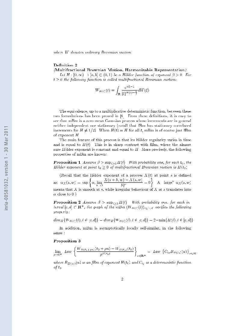
where W denotes ordinary Brownian motion.De�nition 2(Multifractional Brownian Motion, Harmonizable Representation)Let H : [0;1)! [a; b] � (0; 1) be a H�older function of exponent � > 0. Fort � 0 the following function is called multifractional Brownian motion:WH(t)(t) = ZR eit��1j�jH(t)+ 12 dW (�)The equivalence, up to a multiplicative deterministic function, between thesetwo formulations has been proved in [6]. From these de�nitions, it is easy tosee that mBm is a zero mean Gaussian process whose increments are in generalneither independent nor stationary (recall that fBm has stationary correlatedincrements for H 6= 1=2). When H(t) = H for all t, mBm is of course just fBmof exponent H .The main feature of this process is that its H�older regularity varies in timeand is equal to H(t). This is in sharp contrast with fBm, where the almostsure H�older exponent is constant and equal to H . More precisely, the followingproperties of mBm are known:Proposition 1 Assume � > supt�0H(t). With probability one, for each t0, theH�older exponent at point t0 � 0 of multifractional Brownian motion is H(t0).(Recall that the H�older exponent of a process X(t) at point s is de�nedas: �X(s; w) = sup��; limh!0 X(s+ h;w)�X(s; w)jhj� = 0�. A \large" �X(s; w)means that X is smooth at s, while irregular behaviour of X at s translates into� close to 0.)Proposition 2 Assume � > supt�0H(t). With probability one, for each in-terval [c; d] � R+, the graph of the mBm (WH(t)(t))t2[c;d] veri�es the followingproperty :dimHfWH(t)(t); t 2 [c; d]g = dimBfWH(t)(t); t 2 [c; d]g = 2�minfH(t); t 2 [c; d]gIn addition, mBm is asymptotically locally self-similar, in the followingsense :Proposition 3lim�!0+ Law �WH(t0+�u)(t0 + �u)�WH(t0)(t0)�H(t0) �u2R+ = Law �Ct0BH(t0)(u)u2R+where BH(t0)(u) is an fBm of exponent H(t0) and Ct0 is a deterministic functionof t0. 2

inria

-005

8103

2, v

ersi

on 1

- 30

Mar

201

1

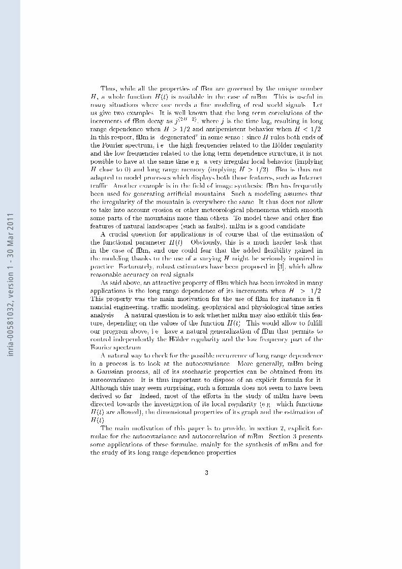
Thus, while all the properties of fBm are governed by the unique numberH , a whole function H(t) is available in the case of mBm. This is useful inmany situations where one needs a �ne modeling of real world signals. Letus give two examples. It is well known that the long term correlations of theincrements of fBm decay as j(2H�2), where j is the time lag, resulting in longrange dependence when H > 1=2 and antipersistent behavior when H < 1=2.In this respect, fBm is \degenerated" in some sense : since H rules both ends ofthe Fourier spectrum, i.e. the high frequencies related to the H�older regularityand the low frequencies related to the long term dependence structure, it is notpossible to have at the same time e.g. a very irregular local behavior (implyingH close to 0) and long range memory (implying H > 1=2). fBm is thus notadapted to model processes which displays both those features, such as Internettra�c. Another example is in the �eld of image synthesis: fBm has frequentlybeen used for generating arti�cial mountains. Such a modeling assumes thatthe irregularity of the mountain is everywhere the same. It thus does not allowto take into account erosion or other meteorological phenomena which smoothsome parts of the mountains more than others. To model these and other �nefeatures of natural landscapes (such as faults), mBm is a good candidate.A crucial question for applications is of course that of the estimation ofthe functional parameter H(t). Obviously, this is a much harder task thatin the case of fBm, and one could fear that the added exibility gained inthe modeling thanks to the use of a varying H might be seriously impaired inpractice. Fortunately, robust estimators have been proposed in [3], which allowreasonable accuracy on real signals.As said above, an attractive property of fBm which has been invoked in manyapplications is the long range dependence of its increments when H > 1=2.This property was the main motivation for the use of fBm for instance in �-nancial engineering, tra�c modeling, geophysical and physiological time seriesanalysis . . . A natural question is to ask whether mBm may also exhibit this fea-ture, depending on the values of the function H(t). This would allow to ful�llour program above, i.e. have a natural generalization of fBm that permits tocontrol independently the H�older regularity and the low frequency part of theFourier spectrum.A natural way to check for the possible occurrence of long range dependencein a process is to look at the autocovariance. More generally, mBm beinga Gaussian process, all of its stochastic properties can be obtained from itsautocovariance. It is thus important to dispose of an explicit formula for it.Although this may seem surprising, such a formula does not seem to have beenderived so far. Indeed, most of the e�orts in the study of mBm have beendirected towards the investigation of its local regularity (e.g. which functionsH(t) are allowed), the dimensional properties of its graph and the estimation ofH(t).The main motivation of this paper is to provide, in section 2, explicit for-mulae for the autocovariance and autocorrelation of mBm. Section 3 presentssome applications of these formulae, mainly for the synthesis of mBm and forthe study of its long range dependence properties.3

inria

-005

8103

2, v

ersi

on 1

- 30

Mar

201

1

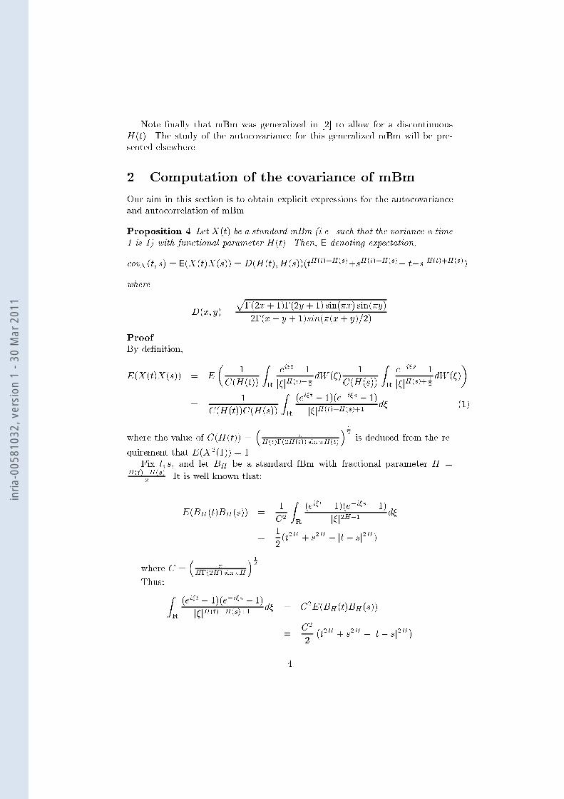
Note �nally that mBm was generalized in [2] to allow for a discontinuousH(t). The study of the autocovariance for this generalized mBm will be pre-sented elsewhere.2 Computation of the covariance of mBmOur aim in this section is to obtain explicit expressions for the autocovarianceand autocorrelation of mBm.Proposition 4 Let X(t) be a standard mBm (i.e. such that the variance a time1 is 1) with functional parameter H(t). Then, E denoting expectation,covX(t; s) = E(X(t)X(s)) = D(H(t); H(s))(tH(t)+H(s)+sH(t)+H(s)�jt�sjH(t)+H(s))where D(x; y) = p�(2x+ 1)�(2y + 1) sin(�x) sin(�y)2�(x+ y + 1)sin(�(x+ y)=2)ProofBy de�nition,E(X(t)X(s)) = E � 1C(H(t)) ZR ei�t � 1j�jH(t)+ 12 dW (�) 1C(H(s)) ZR e�i�s � 1j�jH(s)+ 12 dW (�)�= 1C(H(t))C(H(s)) ZR (ei�t � 1)(e�i�s � 1)j�jH(t)+H(s)+1 d� (1)where the value of C(H(t)) = � �H(t)�(2H(t)) sin �H(t)� 12 is deduced from the re-quirement that E(X2(1)) = 1.Fix t; s, and let BH be a standard fBm with fractional parameter H =H(t)+H(s)2 . It is well known that:E(BH (t)BH(s)) = 1C2 ZR (ei�t � 1)(e�i�s � 1)j�j2H+1 d�= 12(t2H + s2H � jt� sj2H)where C = � �H�(2H) sin�H� 12 .Thus: ZR (ei�t � 1)(e�i�s � 1)j�jH(t)+H(s)+1 d� = C2E(BH(t)BH (s))= C22 �t2H + s2H � jt� sj2H�4

inria

-005

8103

2, v

ersi

on 1

- 30

Mar

201

1

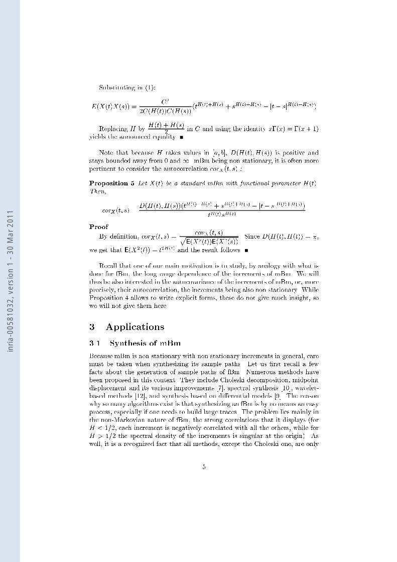
Substituting in (1):E(X(t)X(s)) = C22C(H(t))C(H(s)) (tH(t)+H(s) + sH(t)+H(s) � jt� sjH(t)+H(s))Replacing H by H(t) +H(s)2 in C and using the identity x�(x) = �(x+ 1)yields the announced equality.Note that because H takes values in [a; b], D(H(t); H(s)) is positive andstays bounded away from 0 and1. mBm being non stationary, it is often morepertinent to consider the autocorrelation corX (t; s) :Proposition 5 Let X(t) be a standard mBm with functional parameter H(t).Then,corX(t; s) = D(H(t); H(s))(tH(t)+H(s) + sH(t)+H(s) � jt� sjH(t)+H(s))tH(t)sH(s)ProofBy de�nition, corX(t; s) = covX (t; s)pE(X2(t))E(X2(s)) . Since D(H(t); H(t)) = 12 ,we get that E(X2(t)) = t2H(t) and the result follows.Recall that one of our main motivation is to study, by analogy with what isdone for fBm, the long range dependence of the increments of mBm. We willthus be also interested in the autocovariance of the increments of mBm, or, moreprecisely, their autocorrelation, the increments being also non stationary. WhileProposition 4 allows to write explicit forms, these do not give much insight, sowe will not give them here.3 Applications3.1 Synthesis of mBmBecause mBm is non stationary with non stationary increments in general, caremust be taken when synthesizing its sample paths. Let us �rst recall a fewfacts about the generation of sample paths of fBm. Numerous methods havebeen proposed in this context. They include Choleski decomposition, midpointdisplacement and its various improvements [7], spectral synthesis [10], wavelet-based methods [12], and synthesis based on di�erential models [9]. The reasonwhy so many algorithms exist is that synthesizing an fBm is by no means an easyprocess, especially if one needs to build large traces. The problem lies mainly inthe non-Markovian nature of fBm, the strong correlations that it displays (forH < 1=2, each increment is negatively correlated with all the others, while forH > 1=2 the spectral density of the increments is singular at the origin). Aswell, it is a recognized fact that all methods, except the Choleski one, are only5

inria

-005

8103

2, v

ersi

on 1

- 30

Mar

201

1

approximate. It is not clear however why the unique exact synthesis, throughCholeski decomposition, is not used systematically. It probably stems from thewrong impression that this method is greatly time and memory consuming.While this is true for a plain implementation of the algorithm, several re�ne-ments allow to reduce the time and memory requirements to values comparableto the ones of the \fast" approximate methods. Let us describe in some detailthe principal steps involved in the Choleski decomposition method.Assume we wish to generate samples of an fBm X with exponent H atN equidistant points of [0; 1]. Let DX denote the discrete increments of X ,that is DX(k=N) = X(k=N) � X((k � 1)=N); k = 1; : : :N . These incrementsform a discrete stationary Gaussian process with zero mean, and the statisticalproperties of the vector DXN = (DX(1=N); DX(2=N); : : : ; DX(1)) are entirelydetermined by the autocovariance matrix AN = E(DXN (DXN )T ), where UTdenotes the transpose of U . It is well known that E(DX(i=N)DX((i+k)=N)) =12N2H (jk + 1j2H + jk � 1j2H � 2jkj2H). Since AN is positive de�nite, it may bewritten using its Choleski decomposition as:AN = LNLTN (2)where LN is an invertible lower triangular matrix.Let DYN = (DY (1=N); DY (2=N); : : : ; DY (1)) be an N -samples realizationof a unit variance centered white Gaussian noise. It is easy to see that theautocovariance matrix of the random vector LNDYN is exactly AN . Indeed:E(LNDYN (LNDYN )T ) = LNE(DYN (DYN )T )LTN = AN (3)We may thus set DXN = LNDYN , and generate a realization of the fBm Xas X(k=N) = Pkp=1DX(p=N). Since AN depends only on N and H , it isentirely determined once we have �xed the exponent and the number of pointswe wish to generate. The problem of synthesizing a sample of an fBm is thusreduced to that of computing LN from AN . Note that, so far, we have onlyused the fact that AN is a valid autocovariance matrix, so that it has a Choleskidecomposition. Thus the procedure above may be applied for synthesizing anydiscrete Gaussian process. A direct method for general Choleski factorizationhas complexity O(N3) and requires O(N2) memory. This precludes the use ofthis approach for building large traces, and is the reason usually invoked forthe need of fast approximate methods. However, when the process is stationary(this is why we work withDX rather thanX) and in the common case where thesamples are equi-spaced, the matrix considered is Toeplitz: one can then use fastalgorithms, such as the Schur or Levinson algorithms, which have complexityO(N2) and need O(N) memory. Furthermore, it is possible to do even betterif one forces N to be a power of 2. Such a requirement is common to manymethods (e.g. FFT or dyadic wavelet-based), and is not generally consideredas a major drawback. In this case the doubling Schur algorithm [1] allows toreduce the complexity to O(N(log2(N))2). This is very reasonable and permitsthe exact synthesis of quite large traces (for comparison, spectral methods basedon the FFT have complexity O(N(log2(N))).6

inria

-005

8103

2, v

ersi

on 1

- 30

Mar

201

1

Let us now turn to the synthesis of mBm. The usual technique is based onthe following theorem ([11]):Theorem 1 Let (BH(t))t�0 be an fBm of index H. Then for any interval[a; b] � (0; 1) and K > 0 we have almost surelylimh!0 supa � H;H 0 � bjH 0 �H j < h supt2[0;K] jBH(t)�BH0 (t)j = 0:This result allows to generate a sample path of an mBmX(t) with t 2 [t0; t1]through the following procedure :� Denote Hi = H(ti) for ti = t0 + (t1 � t0) iN ; i = 0 : : :N , where N + 1 isthe number of sample points to be generated.� For a �xed !, synthesize all fBm-s BHi with parameterHi on [t0; t1]. Moreprecisely, we generate one realization of a white noise DYN and computeall the matrices LN (Hi) corresponding to the increments of fBm-s withexponent Hi, as de�ned in (2). We then set DXHiN = LN(Hi)DYN andadd these increments to obtain BHi .� X is then obtained by setting X(ti) = BHi(ti).This procedure has complexityN times the complexity of generating a singlefBm, and needs N times the memory required for the synthesis of an fBm.Thus, if one uses the Schur algorithm, the time complexity is O(N3) and O(N2)memory is needed. In the case the doubling Schur algorithm is used, the timecomplexity falls to O(N2(log2(N))2).Now that we dispose of a formula for the autocovariance of mBm, an al-ternate method may be proposed : one can use the Choleski decompositionto generate directly the samples of an mBm, without synthesizing �rst all the\tangent" fBm-s. Indeed, as said above, the Choleski method may be appliedfor building traces of any discrete Gaussian process. The new method thus usesas a starting point the matrix AN deduced from Proposition 4, and computesthe corresponding matrix LN . Note that, in the case of mBm, there is no pointin working with the increments : since they are not stationary, it is not simplerto obtain LN for the increments than for the original process. In turn, thisimply that one cannot make use of fast algorithms for the decomposition, sothat the time (resp. memory) complexity will be O(N3) (resp. O(N2)). Wethus obtain exactly the same values as in the previous synthesis method whenthe Schur algorithm is used. In particular, the new method is worse than theold one when N may be chosen to be a power of 2. Note however that it isexact, as the previous one was only approximate.3.2 Long range dependenceLet us �rst recall what is usually meant by \long range dependence". Let Y (t)be a stationary process with E(Y 2(t)) = 1. The correlation function of Y (t),7

inria

-005

8103

2, v

ersi

on 1

- 30

Mar

201

1

denoted �, depends only on the lag :�(k) = E(Y (t)Y (t+ k))One possible de�nition of long range dependence is the following [5] :De�nition 3Let Y (t) be a stationary process. Y (t) is said to have long range dependence ifthere exists a number � 2 (�1; 0) and a constant c such that :limk!1 �(k)ck� = 1Some authors use a less stringent de�nition, based on the summability ofthe correlation function :De�nition 4Let Y (t) be a stationary process. Y (t) is said to have long range dependence if+1X0 j�(k)j = +1The increments of fBm yield the most well known example of long rangedependence�e: it is classical that, forH 6= 12 , �(j) is equivalent toH(2H�1)j2H�2when j tends to in�nity. In addition,� 0 < H < 12 : +1X�1 �(k) = 0 and 8 k 6= 0; �(k) < 0 (antipersistant behavior)� H = 12 : �(k) = 0;8 k 6= 0 (independents increments of Brownian motion).� 12 < H < 1 : +1X�1 �(k) = +1 (long range dependence)An alternative de�nition is based on the behavior of the spectral density atthe origin : long range dependence manifests itself through a divergence at lowfrequencies.De�nition 5Let Y (t) be a stationary process. Y (t) is said to have long range dependence ifthere exists a number � 2 (�1; 0) and a constant d such that :lim�!0 f(�)d�� = 1where f denotes the spectral density of Y .8

inria

-005

8103

2, v

ersi

on 1

- 30

Mar

201

1

Again in the case of the increments of fBm, it is well known that the spectraldensity reads :f(�) = 2c(1� cos�) +1Xj=�1(2�j + �)�2H�1; � 2 [��; �]with c = �22� sin(�H)�(2H + 1)As a consequence,f(�) = cj�j1�2H +O(j�jmin(3�2H;2)) when � �! 0and :� H < 12 : f(�) �!�! 0 0.� H > 12 : f(�) �!�! 0 +1.Of course, these de�nitions must be adapted in our case, since mBm doesnot have stationary increments. In particular, it is not straightforward to de-�ne a spectral density for the increments : in general, there are several, nonequivalent, ways to extend the notion of a Fourier spectrum for non stationaryprocesses. For instance, [8] proposes to compute �rst the Wigner-Ville trans-form, which, for a process X(t) yields a function (t; f)!W (t; f), where f rep-resents frequency. An average spectrum is then de�ned by integrating W (t; f)with respect to t. This procedure allows, in the case of fBm, to obtain in asatisfactory way the intuitive fact that the spectrum behaves as 1=jf j2H+1. Al-though it is theoretically possible to follow the same route for mBm, computingthe Wigner-Ville spectrum does not seem to be an easy task when H(t) is anarbitrary H�older function. We will thus rather study the asymptotic behaviorof the correlation function of the increments, corY (t; s). This function dependson both time instants, and the best we can do is to �x one \initial" time, say s,and see what happens when we let t go to in�nity. In doing so, we will obtainan asymptotic behavior conditioned on s, re ecting the fact that the long termcorrelation structure will in general be di�erent for di�erent initial times. Inaddition, and again because of non stationarity, we cannot hope in general thatthe ratio corY (s; s+ h)h� will have a non degenerate limit c for a certain wellchosen �. Rather, we will content ourselves with the fact that corY (s; s+ h)h�stays bounded away from 0 and 1 when h tends to in�nity. We thus set thefollowing de�nitions for long range dependence of non (necessarily) stationaryprocesses :De�nition 6Let Y (t) be a second-order process. Y (t) is said to have long range dependenceif there exists a function �(s) taking values in (�1; 0) such that :8s � 0; corY (s; s+ h) � h�(s)9

inria

-005

8103

2, v

ersi

on 1

- 30

Mar

201

1

when h tends to in�nity.(f(h) � g(h) when h tends to in�nity denotes the property that there exist0 < c < d <1 such that for all su�ciently large h, c � f(h)g(h) � d.)By analogy with De�nition 4, we also consider the weaker condition on thesummability of the autocorrelation :De�nition 7Let Y (t) be a second-order process. Y (t) is said to have long range dependenceif 8� > 0;8s � 0;+1X0 jcorY (s; s+ k�)j = +1Note �nally that since the increments are not stationary, it is importantto consider the correlation function rather than the covariance : for station-ary processes, these di�er by a multiplicative constant, but for mBm (or itsincrements), the ratio covariancecorrelation tends to in�nity when t tends to in�nity.From now on, we assume that H is a non constant function.Proposition 6 (asymptotic behavior of the covariance of mBm)Let X(t) be a standard mBm with functional parameter H(t). Then, when ttends to in�nity, and for all �xed s � 0,H(t) +H(s) < 1) covX (t; s) � 1H(t) +H(s) > 1) covX (t; s) � tH(t)+H(s)�1ProofRecall that, because H(u) varies in [a; b] with 0 < a < b < 1, the renor-malising function D(H(t); H(s)) takes values in an interval [dmin; dmax] with0 < dmin < dmax < 1. Since we are only interested in the order of magni-tude of covX(t; s), we may from now on neglect D(H(t); H(s)) in our compu-tations. The announced result then follows simply from a Taylor expansion of(tH(t)+H(s) + sH(t)+H(s) � jt� sjH(t)+H(s)), where the leading term isD(H(t); H(s))sH(t)+H(s) if H(t) +H(s) < 1and D(H(t); H(s))(H(t) +H(s))stH(t)+H(s)�1 if H(t) +H(s) > 1:(recall that H(t) +H(s) is bounded.)Proposition 7 (asymptotic behavior of the correlation of mBm)Let X(t) be a standard mBm with functional parameter H(t). Then, when ttends to in�nity, and for all �xed s � 0,H(t) +H(s) < 1) corX (t; s) � t�H(t)H(t) +H(s) > 1) corX (t; s) � tH(s)�110

inria

-005

8103

2, v

ersi

on 1

- 30

Mar

201

1

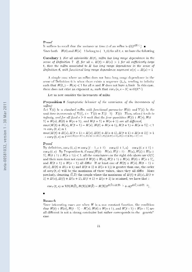
ProofIt su�ces to recall that the variance at time t of an mBm is O(t2H(t)).Since both �H(t) andH(s)�1 belong to (�1; 0) for all t; s, we have the followingCorollary 1 For all admissible H(t), mBm has long range dependence in thesense of De�nition 7. If, for all s, H(t) + H(s) > 1 for all su�ciently larget, then the mBm associated to H has long range dependence in the sense ofDe�nition 6, with functional long range dependence exponent �(s) = H(s)� 1.A simple case where an mBm does not have long range dependence in thesense of De�nition 6 is when there exists a sequence (tn)n tending to in�nitysuch that H(tn) +H(s) < 1 for all n and H does not have a limit. In this case,there does not exist an exponent �s such that corY (s; s+ h) = O(h�s).Let us now consider the increments of mBm.Proposition 8 (asymptotic behavior of the covariance of the increments ofmBm)Let X(t) be a standard mBm with functional parameter H(t) and Y (t) be theunit time increments of X(t), i.e. Y (t) = X(t+1)�X(t). Then, when t tends toin�nity, and for all �xed s � 0 such that the four quantities H(t)+H(s); H(t+1) +H(s); H(t) +H(s+ 1), and H(t+ 1) +H(s+ 1) are all di�erent,max(H(t) +H(s); H(t+ 1) +H(s); H(t) +H(s+ 1); H(t+ 1) +H(s+ 1)) < 1) covY (t; s) � 1max(H(t) +H(s); H(t+ 1) +H(s); H(t) +H(s+ 1); H(t+ 1) +H(s+ 1)) > 1) covY (t; s) � tmax(H(t)+H(s);H(t+1)+H(s);H(t)+H(s+1);H(t+1)+H(s+1))�1ProofBy de�nition, covY (t; s) = covX(t+ 1; s+ 1)� covX (t+1; s)� covX(t; s+ 1)+covX(t; s). By Proposition 6, if max(H(t)+H(s); H(t+1)+H(s); H(t)+H(s+1); H(t+1)+H(s+1)) < 1, all the covariances on the right side above are O(1)and their sum does not cancel if H(t)+H(s); H(t+1)+H(s); H(t)+H(s+1),and H(t + 1) +H(s + 1) all di�er. If at least one of H(t) +H(s); H(t + 1) +H(s); H(t) +H(s+ 1) and H(t+ 1) +H(s+ 1)) is greater than one, the orderof covY (t; s) will be the maximum of these values, since they all di�er. Moreprecisely, denoting (t; s) the couple where the maximum of H(t) +H(s); H(t+1) +H(s); H(t) +H(s+ 1); H(t+ 1) +H(s+ 1) is attained, we have that :covY (t; s) = sD(H(t); H(s))(H(t) +H(s))tH(t)+H(s)�1 + o(tH(t)+H(s)�1):RemarkSince interesting cases are when H is a non constant function, the conditionthat H(t)+H(s); H(t+1)+H(s); H(t)+H(s+1), and H(t+1)+H(s+1) areall di�erent is not a strong constraint but rather corresponds to the \generic"case. 11

inria

-005

8103

2, v

ersi

on 1

- 30

Mar

201

1

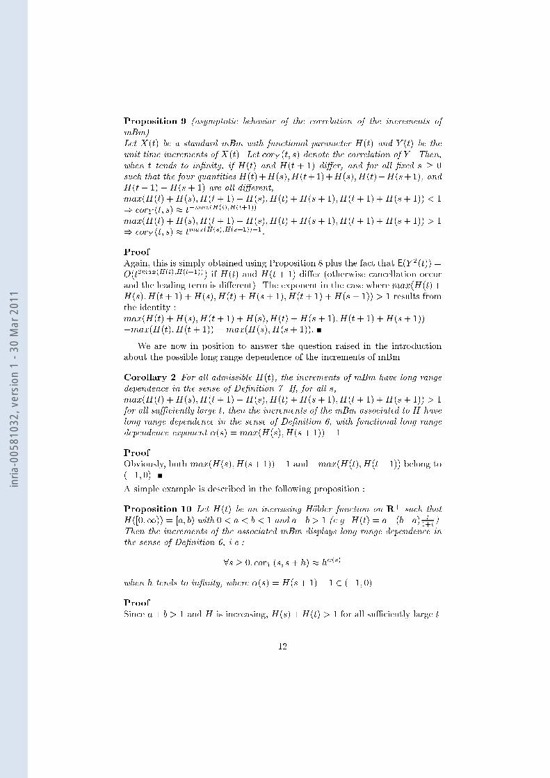
Proposition 9 (asymptotic behavior of the correlation of the increments ofmBm)Let X(t) be a standard mBm with functional parameter H(t) and Y (t) be theunit time increments of X(t). Let corY (t; s) denote the correlation of Y . Then,when t tends to in�nity, if H(t) and H(t + 1) di�er, and for all �xed s � 0such that the four quantities H(t)+H(s); H(t+1)+H(s); H(t)+H(s+1), andH(t+ 1) +H(s+ 1) are all di�erent,max(H(t) +H(s); H(t+ 1) +H(s); H(t) +H(s+ 1); H(t+ 1) +H(s+ 1)) < 1) corY (t; s) � t�max(H(t);H(t+1))max(H(t) +H(s); H(t+ 1) +H(s); H(t) +H(s+ 1); H(t+ 1) +H(s+ 1)) > 1) corY (t; s) � tmax(H(s);H(s+1))�1:ProofAgain, this is simply obtained using Proposition 8 plus the fact that E(Y 2(t)) =O(t2max(H(t);H(t+1))) if H(t) and H(t + 1) di�er (otherwise cancellation occurand the leading term is di�erent). The exponent in the case where max(H(t)+H(s); H(t+ 1) +H(s); H(t) +H(s+ 1); H(t+ 1) +H(s+ 1)) > 1 results fromthe identity :max(H(t) +H(s); H(t+ 1) +H(s); H(t) +H(s+ 1); H(t+ 1) +H(s+ 1))�max(H(t); H(t+ 1)) = max(H(s); H(s+ 1)):We are now in position to answer the question raised in the introductionabout the possible long range dependence of the increments of mBm.Corollary 2 For all admissible H(t), the increments of mBm have long rangedependence in the sense of De�nition 7. If, for all s,max(H(t) +H(s); H(t+ 1) +H(s); H(t) +H(s+ 1); H(t+ 1) +H(s+ 1)) > 1for all su�ciently large t, then the increments of the mBm associated to H havelong range dependence in the sense of De�nition 6, with functional long rangedependence exponent �(s) = max(H(s); H(s+ 1))� 1.ProofObviously, both max(H(s); H(s+1))� 1 and �max(H(t); H(t+1)) belong to(�1; 0).A simple example is described in the following proposition :Proposition 10 Let H(t) be an increasing H�older function on R+ such thatH([0;1)) = [a; b) with 0 < a < b < 1 and a+b > 1 (e.g. H(t) = a+(b�a) t1+t ).Then the increments of the associated mBm displays long range dependence inthe sense of De�nition 6, i.e.:8s � 0; corY (s; s+ h) � h�(s)when h tends to in�nity, where �(s) = H(s+ 1)� 1 2 (�1; 0).ProofSince a+ b > 1 and H is increasing, H(s) +H(t) > 1 for all su�ciently large t.12

inria

-005

8103

2, v

ersi

on 1

- 30

Mar

201

1

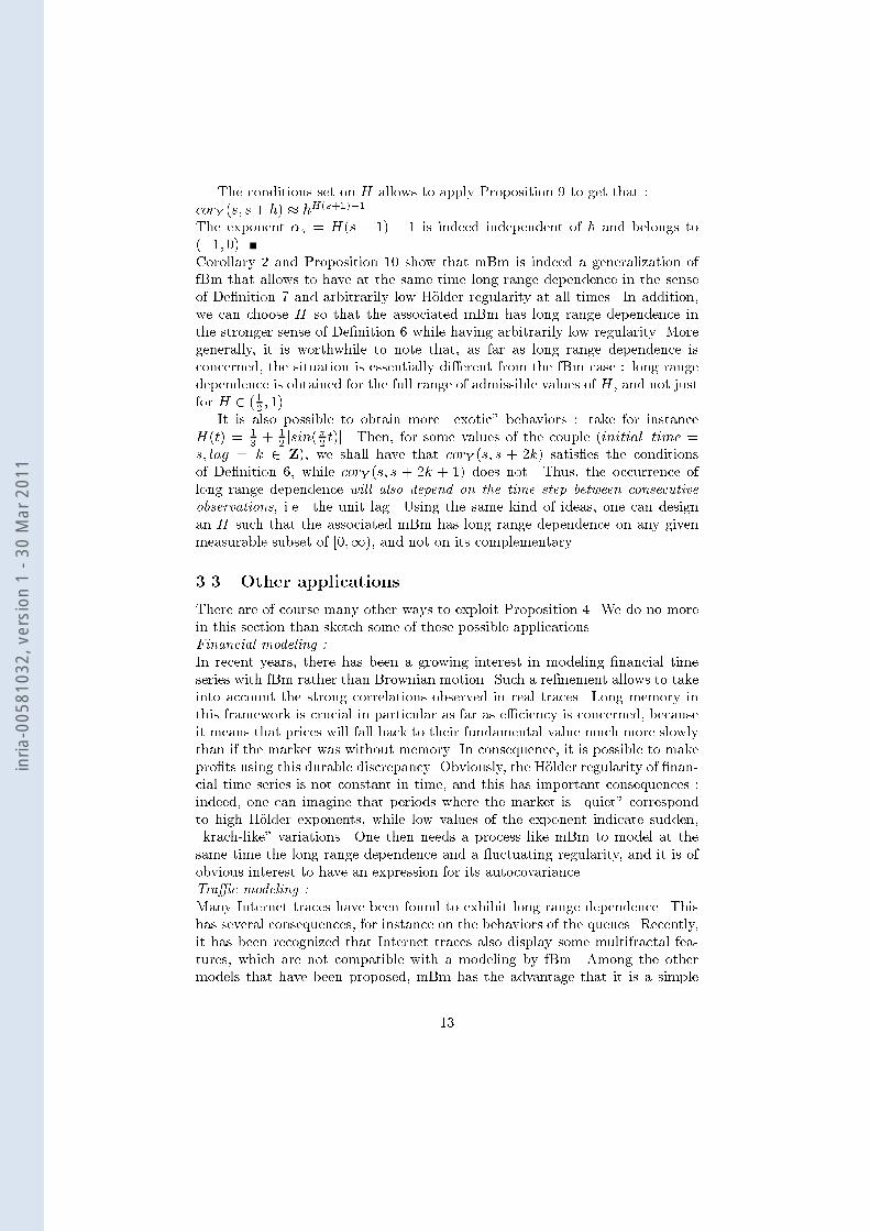
The conditions set on H allows to apply Proposition 9 to get that :corY (s; s+ h) � hH(s+1)�1The exponent �s = H(s + 1) � 1 is indeed independent of h and belongs to(�1; 0).Corollary 2 and Proposition 10 show that mBm is indeed a generalization offBm that allows to have at the same time long range dependence in the senseof De�nition 7 and arbitrarily low H�older regularity at all times. In addition,we can choose H so that the associated mBm has long range dependence inthe stronger sense of De�nition 6 while having arbitrarily low regularity. Moregenerally, it is worthwhile to note that, as far as long range dependence isconcerned, the situation is essentially di�erent from the fBm case : long rangedependence is obtained for the full range of admissible values of H , and not justfor H 2 ( 12 ; 1).It is also possible to obtain more \exotic" behaviors : take for instanceH(t) = 13 + 12 jsin(�2 t)j. Then, for some values of the couple (initial time =s; lag = k 2 Z), we shall have that corY (s; s + 2k) satis�es the conditionsof De�nition 6, while corY (s; s + 2k + 1) does not. Thus, the occurrence oflong range dependence will also depend on the time step between consecutiveobservations, i.e. the unit lag. Using the same kind of ideas, one can designan H such that the associated mBm has long range dependence on any givenmeasurable subset of [0;1), and not on its complementary.3.3 Other applicationsThere are of course many other ways to exploit Proposition 4. We do no morein this section than sketch some of these possible applications.Financial modeling :In recent years, there has been a growing interest in modeling �nancial timeseries with fBm rather than Brownian motion. Such a re�nement allows to takeinto account the strong correlations observed in real traces. Long memory inthis framework is crucial in particular as far as e�ciency is concerned, becauseit means that prices will fall back to their fundamental value much more slowlythan if the market was without memory. In consequence, it is possible to makepro�ts using this durable discrepancy. Obviously, the H�older regularity of �nan-cial time series is not constant in time, and this has important consequences :indeed, one can imagine that periods where the market is \quiet" correspondto high H�older exponents, while low values of the exponent indicate sudden,\krach-like" variations. One then needs a process like mBm to model at thesame time the long range dependence and a uctuating regularity, and it is ofobvious interest to have an expression for its autocovariance.Tra�c modeling :Many Internet traces have been found to exhibit long range dependence. Thishas several consequences, for instance on the behaviors of the queues. Recently,it has been recognized that Internet traces also display some multifractal fea-tures, which are not compatible with a modeling by fBm. Among the othermodels that have been proposed, mBm has the advantage that it is a simple13

inria

-005

8103

2, v

ersi

on 1

- 30

Mar

201

1

generalization of fBm, and that, thanks to the analysis above, it allows to ex-plain both the long range dependence and the wildly varying local regularity.With a right choice of H(t), we can model accurately the multifractal propertiesof tra�c traces, have the correct long range dependence exponent, and even ac-commodate the fact that di�erent experiments sometimes give slightly di�erentsuch exponents. This can be explained by non stationarity : depending on boththe initial time and the unit lag, one will indeed observe di�erent asymptoticbehaviors. With the simple case investigated in Proposition 10, one can modela tra�c where the long range dependence exponent exists in a generalized senseat all times and is an increasing function of the instant chosen for the beginningof the observations.Finally, Proposition 4 could also serve as a basis for new estimation proce-dures, and for optimal sampling of mBm.References[1] G.S. Ammar and W.B. Gragg, Superfast solution of real positive de�ni-tive Toeplitz systems, SIAM J. Matrix Anal. Appl., 9(1988), 61-76.[2] A. Ayache, J. L�evy V�ehel, The generalized Multifractional BrownianMotion, Th�eor�eme Limites et Longue M�emoire en Statistique, CIRM,Marseille, Novembre 1998.[3] A. Benassi, S. Cohen, J. Istas, Identifying the multifractional functionof a Gaussian process, Stat. and Prob. Letter 39, 337-345.[4] A. Benassi, S. Ja�ard, D. Roux, Gaussian processes and pseudo-di�erential elliptic operators, Rev. Mat. Iberoamericana, 13 (1), 19-89.[5] J. Beran, Statistics for Long-Memory Processes (Chapman & Hall,1994).[6] S. Cohen, From self-similarity to local self-similarity : the estima-tion problem, in Fractals: Theory and Applications in EngineeringM. Dekking, J. L�evy V�ehel, E. Lutton and C. Tricot (Eds). SpringerVerlag, 1999.[7] M.M. Daniel and A.S. Willski, Modeling and estimation of fractionalBrownian motion using multiresolution stochastic processes, Fractalsin Engineering, J. L�evy V�ehel, E. Lutton and C. Tricot Eds (SpringerVerlag 1997).[8] P. Flandrin, On the spectrum of Fractional Brownian Motions, IEEETr. Inf. Theory, 35(1989), 197-199.[9] M.S. Kesner, 1/f noises, Proc. IEEE, 70(1974), 212-218.14

inria

-005

8103

2, v

ersi

on 1

- 30

Mar

201

1

[10] L.M. Kaplan, C.C.J. Kuo, An improved method for 2-D self-similarimage synthesis, IEEE Tr. Image Proc., 5(1996), 754-761.[11] R. Peltier, J. L�evy V�ehel, Multifractional Brownian Motion: de�nitionand preliminary results, Inria research report No. 2645, 1995.[12] G.W. Wornell, Signal Processing with Fractals (Prentice Hall, 1996).

15

inria

-005

8103

2, v

ersi

on 1

- 30

Mar

201

1