Functional Covariance Networks: Obtaining Resting-StateNetworks from Intersubject Variability

Paul A. Taylor,1 Suril Gohel,1 Xin Di,1 Martin Walter,2,3 and Bharat B. Biswal1

Abstract

In this study, we investigate a new approach for examining the separation of the brain into resting-state networks(RSNs) on a group level using resting-state parameters (amplitude of low-frequency fluctuation [ALFF], fractionalALFF [fALFF], the Hurst exponent, and signal standard deviation). Spatial independent component analysis isused to reveal covariance patterns of the relevant resting-state parameters (not the time series) across subjectsthat are shown to be related to known, standard RSNs. As part of the analysis, nonresting state parameters arealso investigated, such as mean of the blood oxygen level-dependent time series and gray matter volume fromanatomical scans. We hypothesize that meaningful RSNs will primarily be elucidated by analysis of theresting-state functional connectivity (RSFC) parameters and not by non-RSFC parameters. First, this shows thepresence of a common influence underlying individual RSFC networks revealed through low-frequency flucta-tion (LFF) parameter properties. Second, this suggests that the LFFs and RSFC networks have neurophysiologicalorigins. Several of the components determined from resting-state parameters in this manner correlate stronglywith known resting-state functional maps, and we term these ‘‘functional covariance networks’’.

Key words: amplitude of low-frequency fluctuation (ALFF); fractional ALFF (fALFF); functional MRI (fMRI);Hurst exponent; resting state; spontaneous neuronal activity

Introduction

Resting-state functional connectivity (RSFC) has be-come an increasingly popular technique of functional

magnetic resonance imaging (fMRI). As first proposed byBiswal et al. (1995), in the absence of external stimulus, low-frequency fluctuations (LFFs) in the blood oxygenationlevel-dependent (BOLD) MR signal can be used to revealbrain networks (Greicius et al., 2003; Lowe et al., 1998;Xiong et al., 1999). Several resting-state networks (RSNs)have since been identified, such as the sensorimotor, execu-tive control, visual, and default mode networks (DMN)(Beckmann et al., 2005; Damoiseaux et al., 2006; Raichleet al., 2001; Seeley et al., 2007). Methods for determiningthese networks include seed-based correlations and indepen-dent component analysis (ICA) of voxel time series (Calhounet al., 2002; Kiviniemi et al., 2003; McKeown et al., 1998).

Though RSFC has been widely used, to date no completetheoretical or physiological explanations for the importanceof these specific low frequencies (which correspond tolengthy timescales of 10–100 sec) have been given. Moreover,

in some cases, it has been suggested that signal sources aresignificantly cardiological, respiratory, or vascular in nature(Birn et al., 2006; Chang et al., 2009; Shmueli et al., 2007;van Buuren et al., 2009; Wise et al., 2004). However, impor-tant studies have shown that RSFC cannot be explained solelyby these sources: (1) filtering for cardiac and respiratory com-ponents leaves a strong LFF signal, from which RSNs aredetected (Biswal et al., 1995; De Luca et al., 2006); (2) in dis-ease studies, clinical subjects and healthy controls with simi-lar cardiac and respiratory patterns have shown significantRSFC differences in specific ROIs ( Jones et al., 2010).

Several RSFC parameters have been developed, such as theamplitude of LFFs (ALFF) (Zang et al., 2007), fractional ALFF(fALFF) (Zou et al., 2008), and the Hurst exponent (Bullmoreet al., 2004; Maxim et al., 2005). These have been shown to beuseful in representing resting-state MRI properties on avoxel- and region-wise basis in several studies of healthyand diseased populations. The test–retest reliabilities ofALFF and fALFF have also been shown to be moderate tohigh, particularly in gray matter (GM) (Zuo et al., 2010).While the significantly higher performance of each parameter

1Department of Radiology, UMDNJ-New Jersey Medical School, Newark, New Jersey.2Department of Psychiatry, University of Magdeburg, Magdeburg, Germany.3Leibniz Institute for Neurobiology, Magdeburg, Germany.

BRAIN CONNECTIVITYVolume 2, Number 4, 2012ª Mary Ann Liebert, Inc.DOI: 10.1089/brain.2012.0095

203

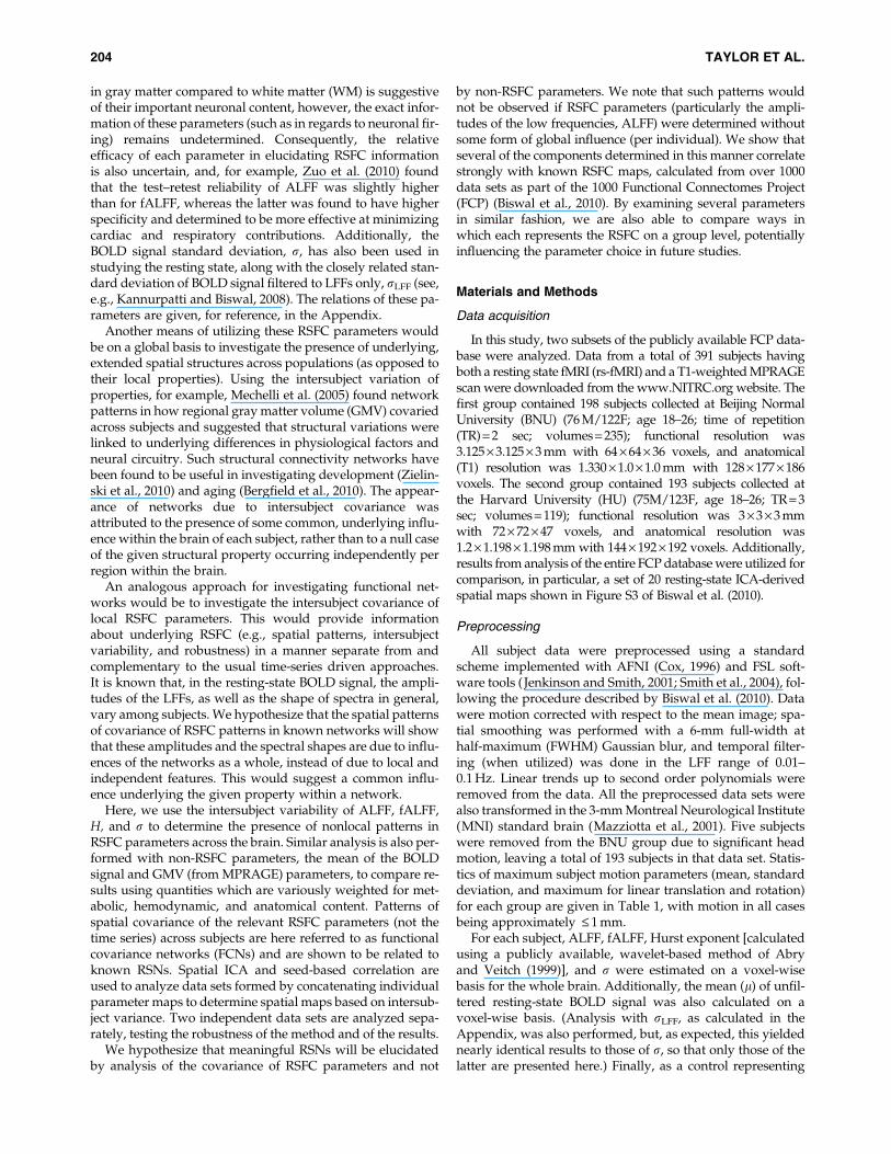
in gray matter compared to white matter (WM) is suggestiveof their important neuronal content, however, the exact infor-mation of these parameters (such as in regards to neuronal fir-ing) remains undetermined. Consequently, the relativeefficacy of each parameter in elucidating RSFC informationis also uncertain, and, for example, Zuo et al. (2010) foundthat the test–retest reliability of ALFF was slightly higherthan for fALFF, whereas the latter was found to have higherspecificity and determined to be more effective at minimizingcardiac and respiratory contributions. Additionally, theBOLD signal standard deviation, r, has also been used instudying the resting state, along with the closely related stan-dard deviation of BOLD signal filtered to LFFs only, rLFF (see,e.g., Kannurpatti and Biswal, 2008). The relations of these pa-rameters are given, for reference, in the Appendix.

Another means of utilizing these RSFC parameters wouldbe on a global basis to investigate the presence of underlying,extended spatial structures across populations (as opposed totheir local properties). Using the intersubject variation ofproperties, for example, Mechelli et al. (2005) found networkpatterns in how regional gray matter volume (GMV) covariedacross subjects and suggested that structural variations werelinked to underlying differences in physiological factors andneural circuitry. Such structural connectivity networks havebeen found to be useful in investigating development (Zielin-ski et al., 2010) and aging (Bergfield et al., 2010). The appear-ance of networks due to intersubject covariance wasattributed to the presence of some common, underlying influ-ence within the brain of each subject, rather than to a null caseof the given structural property occurring independently perregion within the brain.

An analogous approach for investigating functional net-works would be to investigate the intersubject covariance oflocal RSFC parameters. This would provide informationabout underlying RSFC (e.g., spatial patterns, intersubjectvariability, and robustness) in a manner separate from andcomplementary to the usual time-series driven approaches.It is known that, in the resting-state BOLD signal, the ampli-tudes of the LFFs, as well as the shape of spectra in general,vary among subjects. We hypothesize that the spatial patternsof covariance of RSFC patterns in known networks will showthat these amplitudes and the spectral shapes are due to influ-ences of the networks as a whole, instead of due to local andindependent features. This would suggest a common influ-ence underlying the given property within a network.

Here, we use the intersubject variability of ALFF, fALFF,H, and r to determine the presence of nonlocal patterns inRSFC parameters across the brain. Similar analysis is also per-formed with non-RSFC parameters, the mean of the BOLDsignal and GMV (from MPRAGE) parameters, to compare re-sults using quantities which are variously weighted for met-abolic, hemodynamic, and anatomical content. Patterns ofspatial covariance of the relevant RSFC parameters (not thetime series) across subjects are here referred to as functionalcovariance networks (FCNs) and are shown to be related toknown RSNs. Spatial ICA and seed-based correlation areused to analyze data sets formed by concatenating individualparameter maps to determine spatial maps based on intersub-ject variance. Two independent data sets are analyzed sepa-rately, testing the robustness of the method and of the results.

We hypothesize that meaningful RSNs will be elucidatedby analysis of the covariance of RSFC parameters and not

by non-RSFC parameters. We note that such patterns wouldnot be observed if RSFC parameters (particularly the ampli-tudes of the low frequencies, ALFF) were determined withoutsome form of global influence (per individual). We show thatseveral of the components determined in this manner correlatestrongly with known RSFC maps, calculated from over 1000data sets as part of the 1000 Functional Connectomes Project(FCP) (Biswal et al., 2010). By examining several parametersin similar fashion, we are also able to compare ways inwhich each represents the RSFC on a group level, potentiallyinfluencing the parameter choice in future studies.

Materials and Methods

Data acquisition

In this study, two subsets of the publicly available FCP data-base were analyzed. Data from a total of 391 subjects havingboth a resting state fMRI (rs-fMRI) and a T1-weighted MPRAGEscan were downloaded from the www.NITRC.org website. Thefirst group contained 198 subjects collected at Beijing NormalUniversity (BNU) (76 M/122F; age 18–26; time of repetition(TR) = 2 sec; volumes = 235); functional resolution was3.125 · 3.125 · 3 mm with 64 · 64 · 36 voxels, and anatomical(T1) resolution was 1.330 · 1.0 · 1.0 mm with 128 · 177 · 186voxels. The second group contained 193 subjects collected atthe Harvard University (HU) (75M/123F, age 18–26; TR = 3sec; volumes = 119); functional resolution was 3 · 3 · 3 mmwith 72 · 72 · 47 voxels, and anatomical resolution was1.2 · 1.198 · 1.198 mm with 144 · 192 · 192 voxels. Additionally,results from analysis of the entire FCP database were utilized forcomparison, in particular, a set of 20 resting-state ICA-derivedspatial maps shown in Figure S3 of Biswal et al. (2010).

Preprocessing

All subject data were preprocessed using a standardscheme implemented with AFNI (Cox, 1996) and FSL soft-ware tools ( Jenkinson and Smith, 2001; Smith et al., 2004), fol-lowing the procedure described by Biswal et al. (2010). Datawere motion corrected with respect to the mean image; spa-tial smoothing was performed with a 6-mm full-width athalf-maximum (FWHM) Gaussian blur, and temporal filter-ing (when utilized) was done in the LFF range of 0.01–0.1 Hz. Linear trends up to second order polynomials wereremoved from the data. All the preprocessed data sets werealso transformed in the 3-mm Montreal Neurological Institute(MNI) standard brain (Mazziotta et al., 2001). Five subjectswere removed from the BNU group due to significant headmotion, leaving a total of 193 subjects in that data set. Statis-tics of maximum subject motion parameters (mean, standarddeviation, and maximum for linear translation and rotation)for each group are given in Table 1, with motion in all casesbeing approximately £ 1 mm.

For each subject, ALFF, fALFF, Hurst exponent [calculatedusing a publicly available, wavelet-based method of Abryand Veitch (1999)], and r were estimated on a voxel-wisebasis for the whole brain. Additionally, the mean (l) of unfil-tered resting-state BOLD signal was also calculated on avoxel-wise basis. (Analysis with rLFF, as calculated in theAppendix, was also performed, but, as expected, this yieldednearly identical results to those of r, so that only those of thelatter are presented here.) Finally, as a control representing

204 TAYLOR ET AL.

anatomical structure, GMV values (from the MPRAGE/T1weighted images) were computed as well. Similar to the ap-proach implemented by Mechelli et al. (2005), segmentationof the anatomical image was performed using a unified seg-mentation algorithm (Ashburner and Friston, 2000, 2005)implemented in Statistical Parametric Mapping Software(SPM8) with Matlab (MathWorks, Natick, MA). For each ofthe subjects in the HU and BNU groups, the anatomicalMPRAGE image was segmented in to gray matter and trans-formed into MNI 3-mm standard space. An additional mod-ulation step was also performed on the segmented images aspart of the voxel-based morphometry (VBM) processingscheme, to preserve the total amount of gray matter in eachvoxel before and after the transformation into MNI standardspace (Good et al., 2001). The group-wise analysis of the sixvariables of interest is described below (the parameter formu-lations and relations are given in the Appendix).

Calculations of connectivity maps

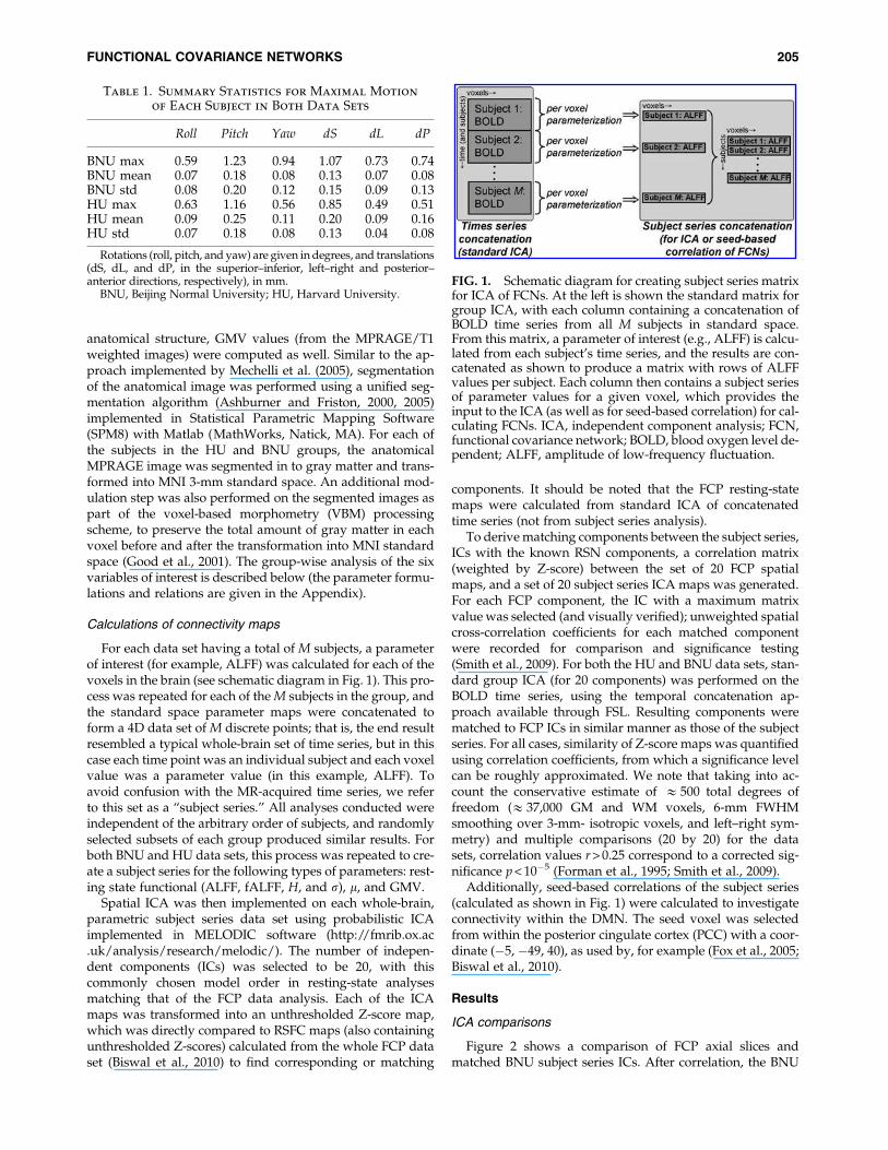
For each data set having a total of M subjects, a parameterof interest (for example, ALFF) was calculated for each of thevoxels in the brain (see schematic diagram in Fig. 1). This pro-cess was repeated for each of the M subjects in the group, andthe standard space parameter maps were concatenated toform a 4D data set of M discrete points; that is, the end resultresembled a typical whole-brain set of time series, but in thiscase each time point was an individual subject and each voxelvalue was a parameter value (in this example, ALFF). Toavoid confusion with the MR-acquired time series, we referto this set as a ‘‘subject series.’’ All analyses conducted wereindependent of the arbitrary order of subjects, and randomlyselected subsets of each group produced similar results. Forboth BNU and HU data sets, this process was repeated to cre-ate a subject series for the following types of parameters: rest-ing state functional (ALFF, fALFF, H, and r), l, and GMV.

Spatial ICA was then implemented on each whole-brain,parametric subject series data set using probabilistic ICAimplemented in MELODIC software (http://fmrib.ox.ac.uk/analysis/research/melodic/). The number of indepen-dent components (ICs) was selected to be 20, with thiscommonly chosen model order in resting-state analysesmatching that of the FCP data analysis. Each of the ICAmaps was transformed into an unthresholded Z-score map,which was directly compared to RSFC maps (also containingunthresholded Z-scores) calculated from the whole FCP dataset (Biswal et al., 2010) to find corresponding or matching

components. It should be noted that the FCP resting-statemaps were calculated from standard ICA of concatenatedtime series (not from subject series analysis).

To derive matching components between the subject series,ICs with the known RSN components, a correlation matrix(weighted by Z-score) between the set of 20 FCP spatialmaps, and a set of 20 subject series ICA maps was generated.For each FCP component, the IC with a maximum matrixvalue was selected (and visually verified); unweighted spatialcross-correlation coefficients for each matched componentwere recorded for comparison and significance testing(Smith et al., 2009). For both the HU and BNU data sets, stan-dard group ICA (for 20 components) was performed on theBOLD time series, using the temporal concatenation ap-proach available through FSL. Resulting components werematched to FCP ICs in similar manner as those of the subjectseries. For all cases, similarity of Z-score maps was quantifiedusing correlation coefficients, from which a significance levelcan be roughly approximated. We note that taking into ac-count the conservative estimate of & 500 total degrees offreedom (& 37,000 GM and WM voxels, 6-mm FWHMsmoothing over 3-mm- isotropic voxels, and left–right sym-metry) and multiple comparisons (20 by 20) for the datasets, correlation values r > 0.25 correspond to a corrected sig-nificance p < 10�5 (Forman et al., 1995; Smith et al., 2009).

Additionally, seed-based correlations of the subject series(calculated as shown in Fig. 1) were calculated to investigateconnectivity within the DMN. The seed voxel was selectedfrom within the posterior cingulate cortex (PCC) with a coor-dinate (�5, �49, 40), as used by, for example (Fox et al., 2005;Biswal et al., 2010).

Results

ICA comparisons

Figure 2 shows a comparison of FCP axial slices andmatched BNU subject series ICs. After correlation, the BNU

FIG. 1. Schematic diagram for creating subject series matrixfor ICA of FCNs. At the left is shown the standard matrix forgroup ICA, with each column containing a concatenation ofBOLD time series from all M subjects in standard space.From this matrix, a parameter of interest (e.g., ALFF) is calcu-lated from each subject’s time series, and the results are con-catenated as shown to produce a matrix with rows of ALFFvalues per subject. Each column then contains a subject seriesof parameter values for a given voxel, which provides theinput to the ICA (as well as for seed-based correlation) for cal-culating FCNs. ICA, independent component analysis; FCN,functional covariance network; BOLD, blood oxygen level de-pendent; ALFF, amplitude of low-frequency fluctuation.

Table 1. Summary Statistics for Maximal Motion

of Each Subject in Both Data Sets

Roll Pitch Yaw dS dL dP

BNU max 0.59 1.23 0.94 1.07 0.73 0.74BNU mean 0.07 0.18 0.08 0.13 0.07 0.08BNU std 0.08 0.20 0.12 0.15 0.09 0.13HU max 0.63 1.16 0.56 0.85 0.49 0.51HU mean 0.09 0.25 0.11 0.20 0.09 0.16HU std 0.07 0.18 0.08 0.13 0.04 0.08

Rotations (roll, pitch, and yaw) are given in degrees, and translations(dS, dL, and dP, in the superior–inferior, left–right and posterior–anterior directions, respectively), in mm.

BNU, Beijing Normal University; HU, Harvard University.

FUNCTIONAL COVARIANCE NETWORKS 205

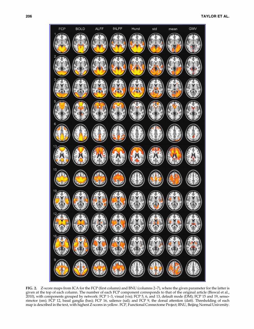
FIG. 2. Z-score maps from ICA for the FCP (first column) and BNU (columns 2–7), where the given parameter for the latter isgiven at the top of each column. The number of each FCP component corresponds to that of the original article (Biswal et al.,2010), with components grouped by network: FCP 1–3, visual (vis); FCP 5, 6, and 13, default mode (DM); FCP 15 and 19, senso-rimotor (sm); FCP 12, basal ganglia (bas); FCP 16, salience (sal); and FCP 9, the dorsal attention (datt). Thresholding of eachmap is described in the text, with highest Z-scores in yellow. FCP, Functional Connectome Project; BNU, Beijing Normal University.

206 TAYLOR ET AL.

ICs were thresholded for visualization, using cluster-basedthresholding with Z > 2.3 and a cluster extent of p < 0.01.The first column represents the FCP maps (with componentnumber shown), followed by the ICs for the standardBOLD time series, ALFF, fALFF, H, r, l, and GMV. [Axialslice numbers were chosen to match those of the Biswalet al. (2010), except for IC 6.] Several known RSNs are repre-sented by individual or groups of FCP components. Relevantones for this study are shown, grouped appropriately, in thefirst columns of Figure 2 (and Fig. 3). The visual network isshown by FCP 1, 2, and 3, with striate and extrastriate por-tions being distinct. The DMN is represented by FCP 5, 6,and 13, with highest Z-scores, respectively, in the ventral–medial prefrontal, the posterior cingulate, and the medial pre-frontal cortices. The sensorimotor network is given by FCP15 and 19 (somatosensory), and FCP 12 shows the basal gan-glia network. FCP 16 corresponds to the anterior insula, partof the salience network, and FCP 9, to the dorsal attention net-work. The associated (unweighted) spatial cross-correlationcoefficient values for the subject series parameters are givenin Table 2. A large overlap of high Z-score regions is observedfor most resting-state parameters, with corresponding corre-lation values r > 0.25; as estimated in the Methods, this corre-lation value corresponds to a corrected significance ofp < 10�5. In many cases, correlation between ICs was muchlarger than r > 0.4.

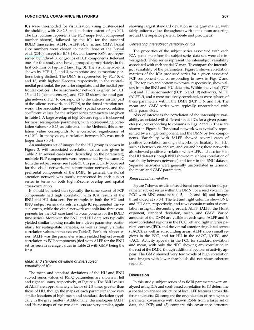
An analogous set of images for the HU group is shown inFigure 3, with associated correlation values also given inTable 2. In several cases (and depending on the parameter),multiple FCP components were represented by the same ICfrom the subject series (see Table 3); this particularly occurredfor the visual network, the sensorimotor network, and theprefrontal components of the DMN. In general, the dorsalattention network was poorly represented by each subjectseries in terms of both high Z-score overlap and spatialcross-correlation.

It should be noted that typically the same subset of FCPcomponents had high correlation with ICA results of theBNU and HU data sets. For example, in both the HU andBNU subject series data sets, a single IC represented the vi-sual cortex, while the visual network was split into three com-ponents for the FCP case (and two components for the BOLDtime series). Moreover, the BNU and HU data sets typicallyyielded similar looking results for a given parameter, partic-ularly for resting-state variables, as well as roughly similarcorrelation values, in most cases (Table 2). For both subject se-ries, fALFF was the parameter which yielded highest overallcorrelation to FCP components (tied with ALFF for the BNUset; as seen in average values in Table 2) with GMV being theleast.

Mean and standard deviation of intersubjectvariability of ICs

The mean and standard deviations of the HU and BNUsubject series values of RSFC parameters are shown in leftand right columns, respectively, of Figure 4. The BNU valuesof ALFF are approximately a factor of 2.5 times greater thanthose of HU, though the maps of each parameter show verysimilar locations of high mean and standard deviation (typi-cally in the gray matter). Additionally, the analogous fALFFand Hurst maps of the two data sets are very similar, again

showing largest standard deviation in the gray matter, withfairly uniform values throughout (with a maximum occurringaround the superior parietal lobule and precuneus).

Correlating intersubject variability of ICs

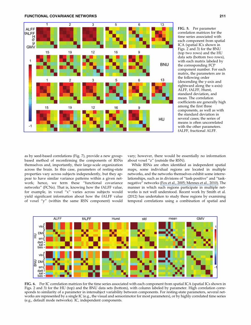
The properties of the subject series associated with eachICA spatial map from the subject series data sets were also in-vestigated. These series represent the intersubject variabilityassociated with each spatial IC map. To compare the intersub-ject variability of the parameters, Figure 5 shows correlationmatrices of the ICA-produced series for a given associatedFCP component (i.e., corresponding to rows in Figs. 2 and3). The top two and bottom two rows, respectively, show val-ues from the BNU and HU data sets. Within the visual (FCP1–3) and HU sensorimotor (FCP 15 and 19) networks, ALFF,fALFF, H, and r were positively correlated, as were subsets ofthese parameters within the DMN (FCP 5, 6, and 13). Themean and GMV series were typically uncorrelated withother parameters.

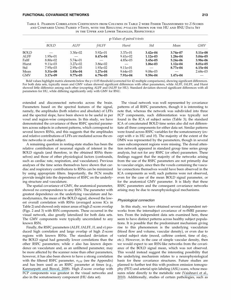
Also of interest is the correlation of the intersubject vari-ability associated with different spatial ICs for a given param-eter (i.e., corresponding to columns in Figs. 2 and 3). These areshown in Figure 6. The visual network was typically repre-sented by a single component, and the DMN by two compo-nents. Variability with fALFF showed several cases ofpositive correlation among networks, particularly for HU,such as between vis and sm, and vis and bas; these networksalso showed positive correlation with ALFF, and also for H inthe HU dataset (though BNU showed much less correlation ofvariability between networks) and for r in the BNU dataset.Separate networks were generally uncorrelated in terms ofthe mean and GMV parameters.

Seed-based correlation

Figure 7 shows results of seed-based correlation for the pa-rameter subject series within the DMN, for a seed voxel in thePCC with MNI coordinate (�5, �49, and 40) and imagesthresholded at r > 0.4. The left and right columns show BNUand HU data, respectively, and rows contain results of corre-lation using (in descending order): ALFF, fALFF, the Hurstexponent, standard deviation, mean, and GMV. Variedamounts of the DMN are visible in each case; fALFF and Hshow correlated regions in the PCC, left and right inferior pa-rietal cortices (IPC), and the ventral anterior cingulated cortex(vACC), as well as surrounding areas; ALFF shows small re-gions in the PCC, and for HU in the vACC, l/rIPC, andvACC. Activity appears in the PCC for standard deviationand mean, with only the rIPC showing any correlation inthe rest of the DMN, though additional regions of activity ap-pear. The GMV showed very few voxels of high correlation(and images with lower thresholds did not show coherentregions).

Discussion

In this study, subject series of rs-fMRI parameters were an-alyzed using ICA and seed-based correlation to: (1) determinea spatial covariance structure of local LFF features across dif-ferent subjects; (2) compare the organization of resting-stateparameter covariance with known RSNs from a large set ofdata, the FCP; and (3) compare this covariance structure

FUNCTIONAL COVARIANCE NETWORKS 207

FIG. 3. Analogous maps to Figure 2 for HU data set. HU, Harvard University.

208 TAYLOR ET AL.

with that of control measures, the mean of the BOLD signaland GMV. We hypothesized that the presence of covariancestructures would suggest a common influence underlyingthe given property within a network. Moreover, in the pres-ence of such organization, comparisons with control parame-ters would test against null hypotheses of whether theinfluence was largely hemodynamic and anatomical.

To create these subject series, the resting parameters ALFF,fALFF, Hurst exponent, and r (which has been used as aresting-state parameter) were calculated across each individ-ual’s whole brain, and the results were concatenated acrossthe group. ICA of the RSFC parameters produced several spa-tial maps, which correlated highly with known resting-statecomponents (defined by FCP data) in both the BNU and

HU sets. Of these parameters, r had lowest overall correlationto FCP RSNs (Table 2), with significantly lower values thanfALFF and Hurst for the HU data set, but not for any otherresting-state parameters for BNU (Table 4). Spatial maps de-rived from the mean of the BOLD signal and GMV tended tohave lower correlation with FCP components, with the great-est overlap with in the visual network, but having signifi-cantly lower correlations to RSNs than any resting-stateparameter (except for mean in BNU, for Hurst, and standarddeviation; Table 4).

Although in this study we have used rs-fMRI informationfrom each subject to look at spatial patterns of connectivity,other investigators have previously used different measuresin a similar manner (i.e., analyzing subject series). For

Table 2. Correlation Coefficients Between The Significant Functional Connectome Project

Components and Each of the Associated Independent Component Analysis Results of the BNUand HU Data Sets are Shown, Grouped by Network

Correlation coefficients

FCP IC BOLD ALFF fALFF Hurst Std Mean GMV(network) BNU; HU BNU; HU BNU; HU BNU; HU BNU; HU BNU; HU BNU; HU

1 (vis) 0.63; 0.75 0.79; 0.72 0.79; 0.78 0.78; 0.76 0.70; 0.63 0.40; 0.43 0.14; 0.222 (vis) 0.63; 0.69 0.78; 0.76 0.70; 0.73 0.64; 0.66 0.74; 0.62 0.40; 0.39 0.11; 0.183 (vis) 0.75; 0.69 0.75; 0.66 0.76; 0.78 0.80; 0.81 0.76; 0.58 0.40; 0.40 0.06; 0.085 (DM) 0.67; 0.61 0.52; 0.44 0.35; 0.50 0.44; 0.51 0.33; 0.40 0.28; 0.28 0.14; 0.136 (DM) 0.64; 0.71 0.34; 0.45 0.40; 0.55 0.18; 0.46 0.11; 0.08 0.13; 0.07 0.08; 0.1413 (DM) 0.67; 0.44 0.53; 0.35 0.55; 0.58 0.37; 0.40 0.41; 0.33 0.29; 0.12 0.03; 0.0615 (sm) 0.72; 0.68 0.72; 0.65 0.64; 0.81 0.36; 0.75 0.53; 0.41 0.29; 0.17 0.02; 0.0319 (sm) 0.66; 0.57 0.69; 0.61 0.66; 0.72 0.34; 0.70 0.47; 0.36 0.22; 0.14 0.03; 0.0512 (bas) 0.66; 0.54 0.29; 0.47 0.28; 0.52 0.40; 0.39 0.41; 0.36 0.26; 0.27 0.28; 0.2516 (sal) 0.73; 0.63 0.42; 0.36 0.59; 0.63 0.43; 0.54 0.27; 0.23 0.27; 0.25 0.12; 0.119 (datt) 0.61; 0.64 0.49; 0.21 0.50; 0.45 0.26; 0.26 0.25; 0.19 0.31; 0.15 0.04; 0.03AVE. 0.67; 0.63 0.57; 0.52 0.57; 0.52 0.46; 0.57 0.45; 0.38 0.29; 0.24 0.10; 0.12ST. DEV. 0.05; 0.09 0.18; 0.17 0.17; 0.13 0.20; 0.18 0.21; 0.18 0.08; 0.12 0.08; 0.07

Mean values of correlation for each column are also shown, for which fALFF shows a maximum for both data sets (tied with H in HU andwith ALFF in BNU sets).

FCP, Functional Connectome Project; IC, independent component; BOLD, blood oxygen level dependent; LFF, low-frequency fluctuation;ALFF, amplitude of LFF; Falff, fractional ALFF; vis, visual; DM, default mode; sm, sensorimotor; datt, dorsal attention; sal, salience; bas, basalganglia; GMV, gray matter volume.

Table 3. The Component Numbers Corresponding to the Spatial Maps in Figures 2 and 3are Shown, Grouped by Network (Defined in Table 2)

IC number

FCP IC BOLD ALFF fALFF Hurst Std Mean GMV(network) BNU; HU BNU; HU BNU; HU BNU; HU BNU; HU BNU; HU BNU; HU

1 (vis) 10; 13 1; 2 1; 2 1; 4 1; 4 1; 6 7; 62 (vis) 6; 19 1; 2 1; 2 1; 4 1; 4 1; 6 7; 63 (vis) 6; 19 1; 2 1; 2 1; 4 1; 4 1; 6 6; 15 (DM) 13; 4 3; 18 6; 6 16; 13 18; 1 5; 15 2; 76 (DM) 4; 5 8; 14 14; 7 15; 6 20; 7 1; 6 15; 1913 (DM) 13; 12 3; 3 6; 6 7; 13 4; 1 2; 15 15; 1915 (sm) 16; 7 2; 1 4; 3 8; 2 2; 17 8; 4 14; 1019 (sm) 15; 20 2; 1 4; 3 8; 2 2; 17 20; 12 14; 1612 (bas) 7; 10 5; 13 19; 15 12; 11 20; 15 9; 16 4; 716 (sal) 5; 20 10; 13 4; 15 19; 20 19; 15 20; 16 4; 169 (datt) 20; 17 2; 1 4; 3 17; 2 2; 7 8; 12 6; 2

Relevant for each column is the repetition of a given component (IC numbers are unrelated across columns and data sets) across differentnetworks (i.e., that the parameter did not separate the networks into separate components), such as for the repeated correlation of IC 5 in theBNU set for fALFF.

FUNCTIONAL COVARIANCE NETWORKS 209

example, He et al. (2007) have used region-wise cortical thick-ness values of subject series for graph theoretical analyses,and Xu et al. (2009) have used gray matter volume for ICA,and Zhang et al. (2011) have used ALFF for seed-based corre-lations. We note that the FCN approach performed in thiswork necessarily has a higher resolution than those ap-proaches, as the RSFC parameters were calculated pervoxel. As large data sets become more easily available, net-work analysis both within and between subjects to aid in un-derstanding functional brain networks should be morefeasible.

Networks from ICA with resting parameters

Spatial ICA of the resting-state parameters produced sev-eral known RSNs, as found through direct comparison withcomponents of the FCP data set. Various components of thevisual network (FCP 1–3) were typically represented as a sin-gle IC, with (left and right) regions of the superior temporalgyrus and insula included in the fALFF and Hurst sets(BNU). Features of the DMN were separated into distinct

components, with extra activation appearing in the medialand inferior frontal gyri, though both Hurst and standard de-viation maps were missing several regions. Bilateral compo-nents of the superior temporal gyrus (FCP 13) typically didnot appear in any components. For the sensorimotor compo-nents (FCP 15 and 19), the left and right precentral gyri andthe cingulate gyri were represented by all RSFC parameters,excepting Hurst for HU, and not by mean and GMV. Thala-mic components of the basal component appeared in mostparameter sets, with a generally smaller spatial extent thanin FCP 12. The salience network in FCP 16 was best repre-sented in ALFF and fALFF for both data sets. Both the inferiorparietal and paracentral lobule features of the dorsal attentionnetwork (FCP 9) were missing for all parameters, and corre-lations were typically quite low (with the same componentfor the sensorimotor network showing highest correlation);possibly weak correlation is shown for the right inferior pari-etal component for HU ALFF, but most likely this componentwas not uniquely identified by the intersubject covariances.

The recapitulation of several known RSNs by ICA of theresting-state parametric subject series (Figs. 2 and 3), as well

FIG. 4. The mean and standard deviation (upper and lower portion of each panel, respectively), of each subject series areshown for the BNU (left column) and HU (right column) data sets for the RSFC parameters: ALFF (A, D), fALFF (B, E),and the Hurst exponent (C, F). Standard deviation is uniformly higher in gray matter than in white matter regions, with similarpatterns of variation observed in both HU and BNU sets in all cases (with ALFF differing in a single brain-wide constant).RSFC, resting-state functional connectivity.

210 TAYLOR ET AL.

as by seed-based correlations (Fig. 7), provide a new group-based method of reconfirming the components of RSNsthemselves and, importantly, their large-scale organizationacross the brain. In this case, parameters of resting-stateproperties vary across subjects independently, but they ap-pear to have similar variance patterns within a given net-work; hence, we term these ‘‘functional covariancenetworks’’ (FCNs). That is, knowing how the fALFF value,for example, in voxel ‘‘x’’ varies across subjects wouldyield significant information about how the fALFF valueof voxel ‘‘y’’ (within the same RSN component) would

vary; however, there would be essentially no informationabout voxel ‘‘z’’ (outside the RSN).

While RSNs are often identified as independent spatialmaps, some individual regions are located in multiplenetworks, and the networks themselves exhibit some interre-lationships, such as in divisions of ‘‘task-positive’’ and ‘‘task-negative’’ networks (Fox et al., 2005; Mennes et al., 2010). Themanner in which such regions participate in multiple net-works is not well understood. Recent work by Smith et al.(2012) has undertaken to study these regions by examiningtemporal correlations using a combination of spatial and

FIG. 5. Per parametercorrelation matrices for thetime series associated witheach component from spatialICA (spatial ICs shown inFigs. 2 and 3) for the BNU(top two rows) and the HUdata sets (bottom two rows),with each matrix labeled bythe corresponding FCPcomponent number. For eachmatrix, the parameters are inthe following order(descending the y-axis andrightward along the x-axis):ALFF, fALFF, Hurst,standard deviation, andmean. The correlationcoefficients are generally highamong the first threecomponents, as well as withthe standard deviation inseveral cases; the series ofmeans is often uncorrelatedwith the other parameters.fALFF, fractional ALFF.

FIG. 6. Per IC correlation matrices for the time series associated with each component from spatial ICA (spatial ICs shown inFigs. 2 and 3) for the HU (top) and the BNU data sets (bottom), with column labeled by parameter. High correlation corre-sponds to similarity of a parameter in intersubject variability between components. For resting-state parameters, several net-works are represented by a single IC (e.g., the visual and sensorimotor for most parameters), or by highly correlated time series(e.g., default mode networks). IC, independent components.

FUNCTIONAL COVARIANCE NETWORKS 211

temporal ICA [a sequence that has been variously imple-mented in, e.g., Seifritz et al. (2002) and Alkan et al. (2011)].The FCN approach discussed here offers another means forstudying the interrelation of spatially independent networkson a group level, via intersubject covariance of resting-stateproperties. In some cases, the variability of parameters inFCNs, which corresponded to separate RSNs, was highly cor-related, as shown in Figure 6 for the visual and sensorimotor

networks, which may suggest higher level organization be-tween these networks. Such possible relations betweenthese and other networks will be investigated further.

RSFC properties

Numerous studies have shown that resting-state BOLDtime series exhibit temporal correlations across spatially

FIG. 7. Spatial maps of significant correlation from seed-based analyses using a seed voxel in the posterior cingulate cortexwith Montreal Neurological Institute coordinate (�5, �49, 40). All images are thresholded at r > 0.4. The first column showsvalues from the BNU set for (A) ALFF, (B) fALFF, (C) Hurst exponent, (D) standard deviation, (E) mean, and (F) GMV,with respective parameters for the HU data set in (G–L).

212 TAYLOR ET AL.

extended and disconnected networks across the brain.Parameters based on the spectral features of the signal,namely, the amplitudes (both relative and absolute) of LFFsand the spectral slope, have been shown to be useful in pervoxel and region-wise comparisons. In this study, we havedemonstrated the covariance of these RSFC spectral parame-ters across subjects in coherent patterns, which correspond toseveral known RSNs, and this suggests that the amplitudesand relative contributions of LFFs are mediated across the en-tire networks in each subject.

A remaining question in resting-state studies has been therelative contribution of neuronal signals of interest in theBOLD signals (and therefore, in the obtained RSNs them-selves) and those of other physiological factors (confounds,such as cardiac rate, respiration, and vasculature). Previousanalyses of the time series themselves have shown that car-diac and respiratory contributions to RSNs can be minimizedby using appropriate filters. Importantly, the FCN resultsprovide insight into the dependence of RSFC on the underly-ing structure and vasculature.

The spatial covariance of GMV, the anatomical parameter,showed no correspondence to any RSN. The parameter withgreatest dependence on the underlying vasculature and he-modynamics, the mean of the BOLD signal, showed the low-est overall correlation with RSNs (averaged across ICs inTable 2) and showed only minor areas of high Z-score overlap(Figs. 2 and 3) with RSN components. These occurred in thevisual network, also greatly lateralized for both data sets.The GMV components were typically uncorrelated to anyknown RSN.

Finally, the RSFC parameters (ALFF, fALFF, H, and r) pro-duced high correlation and large overlap of high Z-scoreregions with known RSNs. The standard deviation ofthe BOLD signal had generally lower correlations than theother RSFC parameters; while r also has known depen-dence on vasculature and, as an unfiltered parameter, maybe more affected by the scanner noise than other parameters,however, it has also been shown to have a strong correlationwith the filtered RSFC parameter, rLFF (see the Appendix)and has been used as an RSFC parameter at times (e.g.,Kannurpatti and Biswal, 2008). High Z-score overlap withFCP components was greatest in the visual networks andalso in the somatosensory component (HU data set).

The visual network was well represented by covariancepatterns of all RSFC parameters, though it is interesting tonote that, whereas the network was subdivided into threeFCP components, such differentiation was typically notfound in the ICA of subject series (Table 3); the standardICA of concatenated BOLD time series also did not differen-tiate all three components for either data set. Similar patternswere found across RSFC variables for the somatosensory (ex-cept with r in HU and H). The majority of the extent of theDMN was represented by the parameters, though in severalcases subcomponent regions were missing. The dorsal atten-tion network appeared in standard group time series groupanalysis, but not for any RSFC (or other) parameters. Thesefindings suggest that the majority of the networks arisingfrom the use of the RSFC parameters are not primarily dueto vascular origin, since then the voxels containing the vascu-lar connections themselves would have been observed in theICA components as well; such patterns were not observed,even for the case of the mean BOLD signal parameter, orfor the anatomical GMV parameter. It is likely that theseRSFC parameters and the consequent covariance networksarising may be due to neurophysiological mechanisms.

Physiological connection

In this study, we have obtained several independent net-works from the intersubject covariance of rs-fMRI parame-ters. From the independent data sets examined here, theseseem to have distinct patterns across healthy subject popula-tions. It is possible that the predominant mechanism givingrise to this phenomenon is the underlying vasculature(blood flow and volume, vascular density), or even due tovaried subject state (mood, caffeine content, time of day,etc.). However, in the case of simple vascular density, thenwe would expect to see RSN-like networks from the covari-ance of the BOLD signal mean, which was not observed.This would instead suggest the interesting possibility thatthe underlying mechanism relates to a neurophysiologicalbasis for these covariance structures. Future studies areplanned to further test this with positron emission tomogra-phy (PET) and arterial spin labeling (ASL) scans, whose mea-sures relate directly to the metabolic rate (Vaishnavi et al.,2010). Additionally, studies of certain pathologies, such as

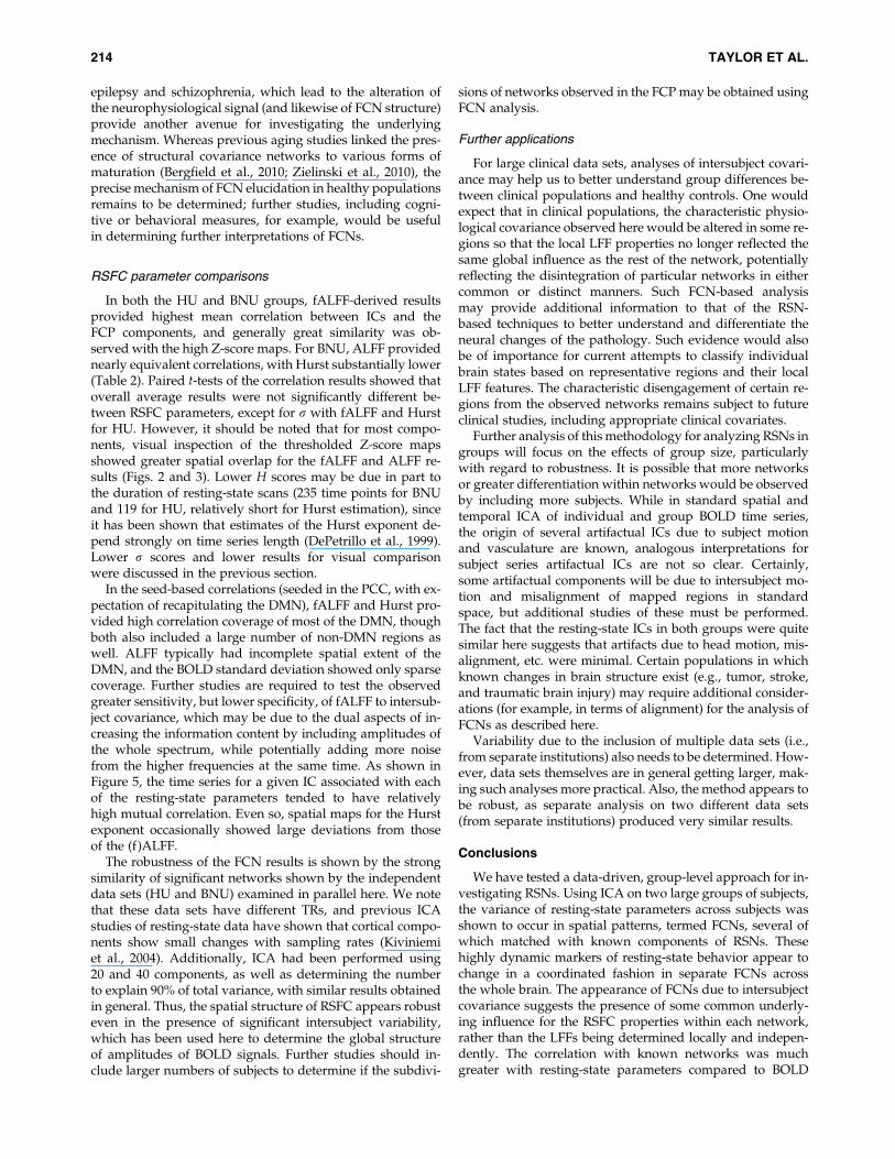
Table 4. Pearson Correlation Coefficients from Columns in Table 2 were Fisher Transformed to Z-Scores

and Compared Using Paired t-Tests, with the Resulting p-values Shown for the HU and BNU Data Set

in the Upper and Lower Triangles, Respectively

p-Values of paired t-tests

BOLD ALFF fALFF Hurst Std Mean GMV

BOLD — 3.30e-02 5.92e-01 3.37e-01 3.42e-04 3.74e-07 5.11e-08ALFF 1.95e-01 — 8.47e-04 9.41e-02 1.12e-03 1.28e-04 5.04e-05Falff 8.80e-02 5.74e-01 — 4.85e-03 3.45e-05 5.24e-06 3.98e-06Hurst 9.11e-03 3.27e-02 3.86e-02 — 1.06e-03 1.12e-04 8.01e-05Std 7.95e-03 2.95e-03 1.93e-02 9.11e-01 — 8.77e-04 6.15e-04Mean 5.31e-08 1.85e-04 1.27e-04 9.64e-03 9.08e-03 — 2.68e-03GMV 3.17e-09 9.77e-05 6.79e-05 7.91e-04 9.59e-04 1.47e-04 —

Bold values highlight matrix elements below the p < 0.05 threshold (corrected for 42 multiple comparisons), showing significant differences.For both data sets, typically mean and GMV values showed significant differences with other parameters, while ALFF, fALFF, and Hurstshowed little difference among each other (excepting ALFF and fALFF for HU). Standard deviation showed significant differences with allparameters for HU, while differing significantly only with GMV for BNU.

FUNCTIONAL COVARIANCE NETWORKS 213

epilepsy and schizophrenia, which lead to the alteration ofthe neurophysiological signal (and likewise of FCN structure)provide another avenue for investigating the underlyingmechanism. Whereas previous aging studies linked the pres-ence of structural covariance networks to various forms ofmaturation (Bergfield et al., 2010; Zielinski et al., 2010), theprecise mechanism of FCN elucidation in healthy populationsremains to be determined; further studies, including cogni-tive or behavioral measures, for example, would be usefulin determining further interpretations of FCNs.

RSFC parameter comparisons

In both the HU and BNU groups, fALFF-derived resultsprovided highest mean correlation between ICs and theFCP components, and generally great similarity was ob-served with the high Z-score maps. For BNU, ALFF providednearly equivalent correlations, with Hurst substantially lower(Table 2). Paired t-tests of the correlation results showed thatoverall average results were not significantly different be-tween RSFC parameters, except for r with fALFF and Hurstfor HU. However, it should be noted that for most compo-nents, visual inspection of the thresholded Z-score mapsshowed greater spatial overlap for the fALFF and ALFF re-sults (Figs. 2 and 3). Lower H scores may be due in part tothe duration of resting-state scans (235 time points for BNUand 119 for HU, relatively short for Hurst estimation), sinceit has been shown that estimates of the Hurst exponent de-pend strongly on time series length (DePetrillo et al., 1999).Lower r scores and lower results for visual comparisonwere discussed in the previous section.

In the seed-based correlations (seeded in the PCC, with ex-pectation of recapitulating the DMN), fALFF and Hurst pro-vided high correlation coverage of most of the DMN, thoughboth also included a large number of non-DMN regions aswell. ALFF typically had incomplete spatial extent of theDMN, and the BOLD standard deviation showed only sparsecoverage. Further studies are required to test the observedgreater sensitivity, but lower specificity, of fALFF to intersub-ject covariance, which may be due to the dual aspects of in-creasing the information content by including amplitudes ofthe whole spectrum, while potentially adding more noisefrom the higher frequencies at the same time. As shown inFigure 5, the time series for a given IC associated with eachof the resting-state parameters tended to have relativelyhigh mutual correlation. Even so, spatial maps for the Hurstexponent occasionally showed large deviations from thoseof the (f)ALFF.

The robustness of the FCN results is shown by the strongsimilarity of significant networks shown by the independentdata sets (HU and BNU) examined in parallel here. We notethat these data sets have different TRs, and previous ICAstudies of resting-state data have shown that cortical compo-nents show small changes with sampling rates (Kiviniemiet al., 2004). Additionally, ICA had been performed using20 and 40 components, as well as determining the numberto explain 90% of total variance, with similar results obtainedin general. Thus, the spatial structure of RSFC appears robusteven in the presence of significant intersubject variability,which has been used here to determine the global structureof amplitudes of BOLD signals. Further studies should in-clude larger numbers of subjects to determine if the subdivi-

sions of networks observed in the FCP may be obtained usingFCN analysis.

Further applications

For large clinical data sets, analyses of intersubject covari-ance may help us to better understand group differences be-tween clinical populations and healthy controls. One wouldexpect that in clinical populations, the characteristic physio-logical covariance observed here would be altered in some re-gions so that the local LFF properties no longer reflected thesame global influence as the rest of the network, potentiallyreflecting the disintegration of particular networks in eithercommon or distinct manners. Such FCN-based analysismay provide additional information to that of the RSN-based techniques to better understand and differentiate theneural changes of the pathology. Such evidence would alsobe of importance for current attempts to classify individualbrain states based on representative regions and their localLFF features. The characteristic disengagement of certain re-gions from the observed networks remains subject to futureclinical studies, including appropriate clinical covariates.

Further analysis of this methodology for analyzing RSNs ingroups will focus on the effects of group size, particularlywith regard to robustness. It is possible that more networksor greater differentiation within networks would be observedby including more subjects. While in standard spatial andtemporal ICA of individual and group BOLD time series,the origin of several artifactual ICs due to subject motionand vasculature are known, analogous interpretations forsubject series artifactual ICs are not so clear. Certainly,some artifactual components will be due to intersubject mo-tion and misalignment of mapped regions in standardspace, but additional studies of these must be performed.The fact that the resting-state ICs in both groups were quitesimilar here suggests that artifacts due to head motion, mis-alignment, etc. were minimal. Certain populations in whichknown changes in brain structure exist (e.g., tumor, stroke,and traumatic brain injury) may require additional consider-ations (for example, in terms of alignment) for the analysis ofFCNs as described here.

Variability due to the inclusion of multiple data sets (i.e.,from separate institutions) also needs to be determined. How-ever, data sets themselves are in general getting larger, mak-ing such analyses more practical. Also, the method appears tobe robust, as separate analysis on two different data sets(from separate institutions) produced very similar results.

Conclusions

We have tested a data-driven, group-level approach for in-vestigating RSNs. Using ICA on two large groups of subjects,the variance of resting-state parameters across subjects wasshown to occur in spatial patterns, termed FCNs, several ofwhich matched with known components of RSNs. Thesehighly dynamic markers of resting-state behavior appear tochange in a coordinated fashion in separate FCNs acrossthe whole brain. The appearance of FCNs due to intersubjectcovariance suggests the presence of some common underly-ing influence for the RSFC properties within each network,rather than the LFFs being determined locally and indepen-dently. The correlation with known networks was muchgreater with resting-state parameters compared to BOLD

214 TAYLOR ET AL.

mean and standard deviation; this suggests that the covary-ing properties of RSNs are significantly greater than thosefrom a purely vascular/hemodynamic response or underly-ing anatomy (i.e., driven by GMV), and that the resting-state parameters themselves (r and Hurst exponent, particu-larly ALFF and fALFF) contain significant information ofneuronal/metabolic responses within the RSNs.

Acknowledgments

The authors would like to thank Doug Ward for severaluseful comments on this article. This work was supportedin part by NIH grants R01 AG032088 and R01 EB000215(B.B.) and DFG-SFB 779 (M.W.).

Author Disclosure Statement

The authors declare no competing financial interests.

References

Abry P, Veitch D. 1999. A wavelet based joint estimator of the pa-rameters of long-range dependence. IEEE Trans Info Theory45:878–897.

Alkan Y, Biswal BB, Taylor PA, Alvarez TL. 2011. Segregation offrontoparietal and cerebellar components within saccade andvergence networks using hierarchical independent compo-nent analysis of fMRI. Vis Neurosci 28:247–261.

Ashburner J, Friston KJ. 2000. Voxel-based morphometry: themethods. NeuroImage 11:805–821.

Ashburner J, Friston KJ. 2005. Unified segmentation. Neuro-image 26:839–851.

Beckmann CF, DeLuca M, Devlin JT, Smith SM. 2005. Investiga-tions into resting-state connectivity using independent com-ponent analysis. Philos Trans R Soc Lond B Biol Sci 360:1001–1013.

Bergfield KL, Hanson KD, Chen K, Teipel SJ, Hampel H, Rapo-port SI, Moeller JR, Alexander GE. 2010. Age-related net-works of regional covariance in MRI gray matter:reproducible multivariate patterns in healthy aging. Neuro-image 49:1750–1759.

Birn RM, Diamond JB, Smith MA, Bandettini PA. 2006. Separat-ing respiratory-variation related fluctuations from neuronal-activity-related fluctuations in fMRI. Neuroimage 31:1536–1548.

Biswal B, Yetkin FZ, Haughton VM, Hyde JS. 1995. Functionalconnectivity in the motor cortex of resting human brainusing echo-planar MRI. Magn Reson Med 34:537–541.

Biswal BB, Mennes M, Zuo XN, Gohel S, Kelly C, Smith SM,Beckmann CF, Adelstein JS, Buckner RL, Colcombe S, Dogo-nowski AM, Ernst M, Fair D, Hampson M, Hoptman MJ,Hyde JS, Kiviniemi VJ, Kotter R, Li SJ, Lin CP, Lowe MJ,Mackay C, Madden DJ, Madsen KH, Margulies DS, MaybergHS, McMahon K, Monk CS, Mostofsky SH, Nagel BJ, Pekar JJ,Peltier SJ, Petersen SE, Riedl V, Rombouts SA, Rypma B,Schlaggar BL, Schmidt S, Seidler RD, Siegle GJ, Sorg C,Teng GJ, Veijola J, Villringer A, Walter M, Wang L,WengXC, Whitfield-Gabrieli S, Williamson P, Windischberger C,Zang YF, Zhang HY, Castellanos FX, Milham MP. 2010.Toward discovery science of human brain function. ProcNatl Acad Sci U S A 107:4734–4739.

Bullmore E, Fadili J, Maxim V, Sendur L, Whitcher B, Suckling J,Brammer M, Breakspear M. 2004. Wavelets and functionalmagnetic resonance imaging of the human brain. Neuroimage23:S234–S249.

Buzsaki G, Draguhn A. 2004. Neuronal oscillations in corticalnetworks. Science 304:1926–1929.

Calhoun VD, Pekar JJ, McGinty VB, Adali T, Watson TD, Pearl-son GD. 2002. Different activation dynamics in multiple neu-ral systems during simulated driving. Hum Brain Mapp16:158–167.

Chang C, Cunningham JP, Glover GH. 2009. Influence of heartrate on the BOLD signal: the cardiac response function. Neu-roimage 44:857–869.

Cox RW. 1996. AFNI: software for analysis and visualization offunctional magnetic resonance neuroimages. Comput BiomedRes 29:162–173.

Damoiseaux JS, Rombouts SA, Barkhof F, Scheltens P, Stam CJ,Smith SM, Beckmann CF. 2006. Consistent resting-state net-works across healthy subjects. Proc Natl Acad Sci U S A103:13848–13853.

De Luca M, Beckmann CF, De Stefano N, Matthews PM, SmithSM. 2006. fMRI resting state networks define distinct modesof long-distance interactions in the human brain. Neuroimage29:1359–1367.

DePetrillo PB, Speers D, Ruttimann UE. 1999. Determining theHurst exponent of fractal time series and its application toelectrocardiographic analysis. Comput Biol Med 29:393–406.

Forman SD, Cohen JD, Fitzgerald M, Eddy WF, Mintun MA,Noll DC. 1995. Improved assessment of significant activa-tion in functional magnetic resonance imaging (fMRI): useof a cluster-size threshold. Magn Reson Med 33:636–647.

Fox MD, Snyder AZ, Vincent JL, Corbetta M, Van Essen DC,Raichle ME. 2005. The human brain is intrinsically organizedinto dynamic, anticorrelated functional networks. Proc NatlAcad Sci U S A 102:9673–9678.

Good CD, Johnsrude I, Ashburner J, Henson RN, Friston KJ,Frackowiak RS. 2001. Cerebral asymmetry and the effects ofsex and handedness on brain structure: a voxel-based mor-phometric analysis of 465 normal adult human brains. Neuro-Image 14:685–700.

Greicius MD, Krasnow B, Reiss AL, Menon V. 2003. Functionalconnectivity in the resting brain: a network analysis of the de-fault mode hypothesis. Proc Natl Acad Sci U S A 100:253–258.

He Y, Chen ZJ, Evans AC. 2007. Small-world anatomical net-works in the human brain revealed by cortical thicknessfrom MRI. Cereb Cortex 17:2407–2419.

Jenkinson M, Smith S. 2001. A global optimisation method for ro-bust affine registration of brain images. Med Image Anal5:143–156.

Jones TB, Bandettini PA, Kenworthy L, Case LK, Milleville SC,Martin A, Birn RM. 2010. Sources of group differences in func-tional connectivity: an investigation applied to autism spec-trum disorder. Neuroimage 49:401–414.

Kannurpatti SS, Biswal BB. 2008. Detection and scaling of task in-duced fMRI-BOLD response using resting state fluctuations.Neuroimage 40:1567–1574.

Kiviniemi V, Kantola J-H, Jauhiainen J, Hyvarinen A, TervonenO. 2003. Independent component analysis of nondeterministicfMRI signal sources. NeuroImage 19:253–260.

Kiviniemi V, Kantola JH, Jauhiainen J, Tervonen O. 2004. Com-parison of methods for detecting nondeterministic BOLD fluc-tuation in fMRI. Magn Reson Imaging 22:197–203.

Lowe MJ, Mock BJ, Sorenson JA. 1998. Functional connectivity insingle and multislice echoplanar imaging using resting statefluctuations. Neuroimage 7:119–132.

Maxim VT, Sendur LS, Fadili J, Suckling J, Gould R, Howard R,Bullmore ET. 2005. Fractional Gaussian noise, functional MRIand Alzheimer’s disease. Neuroimage 25:141–158.

FUNCTIONAL COVARIANCE NETWORKS 215

Mazziotta J, Toga A, Evans A, Fox P, Lancaster J, Zilles K, WoodsR, Paus T, Simpson G, Pike B, Holmes C, Collins L, ThompsonP, MacDonald D, Iacoboni M. Schormann T, Amunts K,Palomero-Gallagher N, Geyer S, Parsons L, Narr K, KabaniN, Le Goualher G, Boomsma D, Cannon T, Kawashima R,Mazoyer B. 2001. A probabilistic atlas and reference systemfor the human brain: International Consortium for Brain Map-ping (ICBM). Philos Trans R Soc Lond B Biol Sci 356:1293–1322.

McKeown MJ, Jung TP, Makeig S, Brown G, Kindermann SS, LeeTW, Sejnowski TJ. 1998. Spatially independent activity pat-terns in functional MRI data during the stroop color-namingtask. Proc Natl Acad Sci U S A 95:803–810.

Mechelli A, Friston KJ, Frackowiak RS, Price CJ. 2005. Structuralcovariance in the human cortex. J Neurosci 25:8303–8310.

Mennes M, Kelly C, Zuo XN, Di Martino A, Biswal B, Xavier Cas-tellanos F, Milham MP. 2010. Inter-individual differences inresting state functional connectivity predict task-inducedBOLD activity. Neuroimage 50:1690–1701.

Raichle ME, MacLeod AM, Snyder AZ, Powers WJ, Gusnard DA,Shulman GL. 2001. A default mode of brain function. ProcNatl Acad Sci U S A 98:676–682.

Salvador R, Martinez A, Pomarol-Clotet E, Gomar J, Vila F, SarroS, Capdevila A, Bullmore E. 2008. A simple view of the brainthrough a frequency-specific functional connectivity measure.Neuroimage 39:279–289.

Seeley WW, Menon V, Schatzberg AF, Keller J, Glover GH,Kenna H, Reiss AL, Greicius MD. 2007. Dissociable intrinsicconnectivity networks for salience processing and executivecontrol. J Neurosci 27:2349–2356.

Shmueli K, van Gelderen P, de Zwart JA, Horovitz SG, FukunagaM, Jansma JM, Duyn JH. 2007. Low-frequency fluctuations inthe cardiac rate as a source of variance in the resting-statefMRI BOLD signal. Neuroimage 38:306–320.

Seifritz E, Esposito F, Hennel F, Mustovic H, Neuhoff JG, BilecenD, Tedeschi G, Scheffler K, Di Salle F. 2002. Spatiotemporalpattern of neural processing in the human auditory cortex.Science 297:1706–1708.

Smith S, Jenkinson M, Woolrich M, Beckmann C, Behrens T,Johansen-Berg H, Bannister P, De Luca M, Drobnjak I, FlitneyD, Niazy R, Saunders J, Vickers J, Zhang Y, De Stefano N,Brady J, Matthews P. 2004. Advances in functional and struc-tural MR image analysis and implementation as FSL. Neuro-Image 23:208–219.

Smith SM, Fox PT, Miller KL, Glahn DC, Fox PM, Mackay CE, Fil-ippini N, Watkins KE, Toro R, Laird AR, Beckmann CF. 2009.Correspondence of the brain’s functional architecture during ac-tivation and rest. Proc Natl Acad Sci U S A 106:13040–13045.

Smith SM, Miller KL, Moeller S, Xu J, Auerbach EJ, WoolrichMW, Beckmann CF, Jenkinson M, Andersson J, Glasser MF,Van Essen DC, Feinberg DA, Yacoub ES, Ugurbil K. 2012.

Temporally-independent functional modes of spontaneousbrain activity. PNAS [Epub ahead of print]; DOI: 10.1073/pnas.1121329109.

Vaishnavi SN, Vlassenko AG, Rundle MM, Snyder AZ, Min-tun MA, Raichle ME. 2010. Regional aerobic glycolysis inthe human brain. Proc Natl Acad Sci U S A 107:17757–17762.

van Buuren M, Gladwin TE, Zandbelt BB, van den Heuvel M,Ramsey NF, Kahn RS, Vink M. 2009. Cardiorespiratory effectson default-mode network activity as measured with fMRI.Hum Brain Mapp 30:3031–3042.

Wise RG, Ide K, Poulin MJ, Tracey I. 2004. Resting fluctuations inarterial carbon dioxide induce significant low frequency vari-ations in BOLD signal. Neuroimage 21:1652–1664.

Xiong J, Parsons LM, Gao JH, Fox PT. 1999. Interregional connec-tivity to primary motor cortex revealed using MRI restingstate images. Hum Brain Mapp 8:151–156.

Xu L, Groth KM, Pearlson G, Schretlen DJ, Calhoun VD. 2009.Source-based morphometry: the use of independent compo-nent analysis to identify gray matter differences with applica-tion to schizophrenia. Hum Brain Mapp 30:711–724.

Zang YF, He Y, Zhu CZ, Cao QJ, Sui MQ, Liang M, Tian LX, JiangTZ, Wang YF. 2007. Altered baseline brain activity in childrenwith ADHD revealed by resting-state functional MRI. BrainDev 29:83–91.

Zhang Z, Liao W, Zuo XN, Wang Z, Yuan C, Jiao Q, Chen H,Biswal BB, Lu G, Liu, Y. 2011. Resting-state brain organizationrevealed by functional covariance networks. PLoS One6:e28817.

Zielinski BA, Gennatas ED, Zhou J, Seeley WW. 2010. Network-level structural covariance in the developing brain. Proc NatlAcad Sci U S A 107:18191–18196.

Zou QH, Zhu CZ, Yang Y, Zuo XN, Long XY, Cao QJ, Wang YF,Zang YF. 2008. An improved approach to detection of ampli-tude of low-frequency fluctuation (ALFF) for resting-statefMRI: fractional ALFF. J Neurosci Methods 172:137–141.

Zuo, X.N., Di Martino, A., Kelly, C., Shehzad, Z.E., Gee, D.G.,Klein, D.F., Castellanos, F.X., Biswal, B.B., Milham, M.P.,2010. The oscillating brain: complex and reliable. Neuroimage49:1432–1445.

Address correspondence to:Paul A. Taylor

Department of RadiologyUMDNJ-New Jersey Medical School

30 Bergen StreetADMC Building 5, Suite 575

Newark 07103, NJ

E-mail: neon.taylor@gmail.com

(Appendix follows/)

216 TAYLOR ET AL.

Appendix

Relations of resting-state BOLD parameters

In this study, several resting-state BOLD parameters are uti-lized during analysis, and their results in elucidating RSNs arecompared. For reference, we briefly describe the mathematicalrelations of the resting-state BOLD parameters here.

For discrete time series, {xn}, with N time points, the follow-ing (complex) Fourier relations hold:

ck = +N� 1

n = 0

xn exp (� ikO0n), (1)

xn =1

N+

N� 1

k = 0

ck exp (ikO0n), (2)

with fundamental frequency O0 = 2p/N. The further interrela-tion of time variables (xn) and frequency variables (ck) is givenby Parseval’s Theorem, which states:

+N� 1

n = 0

jxnj2 =1

N+

N� 1

k = 0

jckj2: (3)

The right hand side (RHS) describes the power spectrum of atime series, with jckj2/N being the power spectral density(PSD) at a given frequency, kO0; the square root of eachterm, jckj/N1/2, is called the amplitude. For a zero-meantime series (or one from which the mean, l, has been sub-tracted) the LHS is simply proportional to the variance, r2:

(N� 1)r2 = +N� 1

n = 0

jxnj2 = +N� 1

k = 0

jckj2

N, (4)

where the RHS was rearranged to reflect the inclusion of thefactor of N in the PSD. From this relation, the standard devi-ation is simply,

r =1ffiffiffiffiffiffiffiffiffiffiffiffi

N� 1p

"+

N� 1

n = 0

jxnj2#1=2

=1ffiffiffiffiffiffiffiffiffiffiffiffi

N� 1p

"+

N� 1

k = 0

jckj2

N

#1=2

_ (5)

Kannurpatti and Biswal (2008) showed that a related parame-ter, the standard deviation of the LFF-filtered time series, washighly correlated with r. This new parameter, called the rest-ing state BOLD fluctuation amplitude (RSFA) or rLFF, can becalculated directly from the frequency relations as:

rLFF =1ffiffiffiffiffiffiffiffiffiffiffiffi

N� 1p

"+b

k = a

jckj2

N

#1=2

, (6)

where a and b correspond to 0.01 and 0.1 Hz, respectively.Instead of PSD terms, Zang et al. (2007) used amplitude

terms of filtered series to formulate a resting-state parameter.As its name denotes, ALFF is simply the sum of amplitudes inthe LFF:

ALFF = +b

k = a

jckjffiffiffiffiNp , (7)

though slight variations of ALFF (such as frequency aver-age and global mean) exist as well. Comparing this termwith the RHS expression for rLFF in Eq. (6), one would expecthigh correlation (and therefore high correlation generallywith r, as the terms are essentially the L1 and L2 norms ofspectral amplitudes (with the latter scaled by [N-1]1/2). Thetwo formulations encode qualitatively similar information.Mathematically, L1 is always greater than or equal to L2,but the latter measure exhibits greater percentage changewhen outliers are introduced to a signal. Therefore, the rela-tive amplitudes of subdivisions of LFFs [which have beenshown to be relevant by, e.g., Buzsaki and Draguhn (2004);Salvador et al. (2008)] may be represented differently by ei-ther L1- or L2-type parameters (i.e., ALFF or r, respectively),and with different susceptibility to noise (greater in the L2

case) FALFF is given simply as the ratio of ALFF to thesum of all frequency amplitudes (up to Nyquist), so that,from Equation (7):

fALFF =

"+b

k = a

jckjffiffiffiffiNp

#"+

N� 1

k = 0

jckjffiffiffiffiNp

#� 1

(8)

It is possible to describe the Hurst exponent in terms of fre-quency properties of the resting-state time series, as well,though most estimation methods utilize other factors, suchas wavelets (Bullmore et al., 2004). For small frequencies,one can show that

PSD(k) / jkj �b: (9)

The spectal slope, b, lies in the range [�1,1] and relates tothe Hurst exponent as b = 2H-1. Thus, the relative contribu-tions of LFF, as can be observed in the spectral slope, affectH directly, whereas r and (f) ALFF depend on summed val-ues of LFFs.

FUNCTIONAL COVARIANCE NETWORKS 217