CLIMATE RESEARCHClim Res

Vol. 13: 61–75, 1999 Published September 7

1. INTRODUCTION

It is generally accepted that the increasing concen-tration of greenhouse gases in the atmosphere can sig-nificantly contribute to the change of climate in thenear future (Houghton et al. 1990, 1992, 1996). Thepotential impacts of the induced climate change onvarious aspects of human environment have been a

source of great concern to scientists and decision-makers (Watson et al. 1996). Many models have beendesigned to assess the potential impacts of climatechange on water resources, vegetation, crop yield(Mearns et al. 1992, Maytín et al. 1995, Semenov &Porter 1995) and so on. However, all these modelsrequire as input future climate scenarios with fine res-olution on both spatial and temporal scales. One of themost important parameters from those scenariosrequired as input for such models is precipitation. It is

© Inter-Research 1999

*E-mail: jcr@fc.ul.pt

A weather generator for obtaining dailyprecipitation scenarios based on

circulation patterns

João Corte-Real*, Hong Xu, Budong Qian

Institute for Applied Science and Technology (ICAT), Faculty of Sciences, University of Lisbon, Campo Grande, 1700 Lisboa, Portugal

ABSTRACT: Based on principal component analysis (PCA) and k-means clustering algorithm, 4 dailycirculation patterns, which are associated with daily precipitation in southern Portugal, have beenidentified from observed daily mean sea level pressure (MSLP) fields over the northeastern Atlanticand western Europe. A weather generator based on daily circulation patterns was calibrated with 3 dif-ferent schemes to simulate daily precipitation occurrence and a 2-parameter gamma distribution wasapplied to generate daily precipitation amounts on rain days in southern Portugal. Parameters of theweather generator were estimated for every month in the winter half of the year (October to March)subject to each of the 4 daily circulation patterns. The weather generator was validated by hindcastusing independent observational data. The synthetic daily precipitation series generated from theweather generator kept most of the important attributes of the observed series, such as the empiricaldistribution of daily precipitation amounts, the autocorrelation structure of the sequence of wet and drydays, the distributions of durations of wet and dry spells, and even the distributions of precipitationtotals on several consecutive days. Furthermore, the daily MSLP fields over the northeastern Atlanticand western Europe simulated by the Hadley Centre’s second generation coupled ocean-atmosphereGCM (HADCM2) control run (HADCM2CON) were validated by comparison with observed dailyMSLP fields. It is clear that HADCM2 is able to reproduce very well daily MSLP fields and their sea-sonal variability over the region. Four daily circulation patterns, associated with daily precipitation inPortugal, identified from the observed daily MSLP fields over the area, were also classified well fromthe simulated daily MSLP fields. The weather generator was then applied to the sequence of daily cir-culation patterns in simulated MSLP fields of HADCM2CON, and validated. Essentially, the conclu-sions of previous validation analysis remained the same in the present case. The results imply that theweather generator can reproduce well important features of the ‘present climate’, including local pre-cipitation in southern Portugal, and can therefore be applied to obtain future precipitation scenariosfrom daily MSLP fields simulated by the 2 transient experiments of HADCM2, HADCM2GHG (green-house gases) and HADCM2SUL (greenhouse gases plus sulphate aerosols). However, it should be keptin mind that the use of the weather generator in obtaining future precipitation scenarios is dependenton the assumption that the present relationship between local precipitation and large-scale atmos-pheric circulation will remain valid in the future changing climate.

KEY WORDS: Weather generator · Downscaling · Precipitation · Daily circulation patterns · SouthernPortugal

Clim Res 13: 61–75, 1999

well known that general circulation models (GCMs)are the most powerful tools for obtaining future climatescenarios. However, GCMs are not good enough tosimulate ‘present climate’ and climate change onregional and local scales, although they are able toreproduce well the large-scale characteristics of at-mospheric circulation. Therefore, it has been widelyagreed that outputs of GCMs cannot be directly usedin impact studies and that downscaling is needed; thisis especially true with respect to precipitation.

Essentially, downscaling approaches can be dividedinto 2 categories: statistical and deterministic. The sta-tistical approaches assume that local climatic parame-ters such as precipitation or temperature are statisti-cally related to large-scale atmospheric circulation andcan be designed in many different ways, such as thesimple analog method, linear and non-linear regres-sion models and canonical correlation analysis. Inaddition, some stochastic models, such as a weathergenerator, can be adopted to generate synthetic timeseries of the climate element based on the observedrelationship between that element and atmosphericcirculation (Wilson et al. 1991, Bardossy & Plate 1992,Bogardi et al. 1993, von Storch et al. 1993, Gyalistras etal. 1994, Schubert 1994, Corte-Real et al. 1995, Schu-bert & Henderson-Sellers 1997). In some cases, anotherstochastic model is calibrated to simulate transitionalregimes of atmospheric circulation (Bardossy & Plate1991, Hay et al. 1992, Wilson et al. 1992). It is apparentthat long-term observational data are needed to trainthe statistical models and that this technique can besuccessful only when close relationships are observedbetween the local climate parameters and large-scaleatmospheric circulation. However, the obvious advan-tageous aspects of the statistical approach are its inex-pensiveness and simplicity. This technique is adoptedin the present paper. For deterministic approaches todownscaling, dynamic limited area models (LAMs) arenested in GCMs and/or in themselves (multiple nest-ing) to simulate climate at high resolution scales beingdriven at each level of nesting by the nearest coarserscale (Giorgi 1990, Giorgi et al. 1992, 1994, Jones et al.1995). This technique has the advantage that simula-tions at progressively smaller grid meshes are dynami-cally consistent with those at larger scales as well aswith the large-scale GCM results; also, regional andlocal forcings (e.g. topography, surface fluxes) aremuch better accounted for in LAMs than in GCMs.However, this approach is computationally verydemanding. A comparison of different downscalingtechniques to estimate climate change in southernEurope can be found in Cubasch et al. (1996). It shouldbe pointed out that variable resolution GCMs and timeslices with high resolution GCMs are also useful down-scaling techniques.

As reported in a previous study (Corte-Real et al.1998), 4 daily circulation patterns have been identifiedfrom daily mean sea level pressure (MSLP) fields overthe northeastern Atlantic and western Europe whichrelate closely to daily precipitation conditions at Évora(southern Portugal). Furthermore, it has been verifiedthat the Hadley Centre’s second generation model(HADCM2) (Johns et al. 1997) reproduces very wellthe abovementioned 4 daily circulation patterns andthat their occurrence regimes couple well with corre-sponding daily precipitation in southern Portugal.Therefore, it is possible to use a weather generatorbased on these circulation patterns to assess future cli-mate change scenarios on a daily scale, and even someaspects of extreme events such as duration of sustainedwet and dry periods. In this paper, a weather generatordesigned to generate time series of daily precipitationat Évora is calibrated based on historical data in thewinter half of the year (October to March). Theweather generator is validated not only on an indepen-dent observational data set, but on daily MSLP fieldsobtained from the control run of the HADCM2 model(HADCM2CON) as well. The results from validationimply that the weather generator, coupled with dailycirculation patterns simulated by HADCM2CON, canreproduce well the ‘present climate’ of local precipita-tion at Évora in the winter half of the year. Therefore, itcan be expected that reasonable future precipitationscenarios in southern Portugal can be obtained byapplying the weather generator to daily MSLP fieldssimulated by HADCM2GHG and HADCM2SUL, 2transient experiments forced respectively by green-house gases and greenhouse gases plus sulphateaerosols. Nevertheless, it should be kept in mind thatthis possibility is only justifiable under the assumptionthat the relationship between local precipitation andlarge-scale atmospheric circulation continues to holdin the future changing climate.

2. DOWNSCALING PROCEDURE: CALIBRATION

2.1. Linkages between local precipitation and large-scale atmospheric circulation

Before calibration of the weather generator, the link-ages between precipitation and large-scale atmos-pheric circulation have to be established. In this study,daily circulation patterns identified from large-scaledaily MSLP fields are used to represent large-scale at-mospheric circulation. As described in Corte-Real et al.(1998), by applying a k-means clustering algorithmcoupled with principal component analysis (PCA) to ob-served daily MSLP fields over the northeastern Atlanticand western Europe, 4 daily circulation patterns have

62

Corte-Real et al.: A weather generator for daily precipitation scenarios

been classified during the period from January 1, 1946,to August 31, 1992. The optimal number of clusters (cir-culation patterns) is determined by an informationmeasure associated with daily precipitation at Évora.The quality of daily precipitation data at Évora is quitegood and some systematic changes related to changesin large-scale atmospheric circulation have been de-tected (Zhang et al. 1997, Corte-Real et al. 1998). Thedetails of the clustering technique and the circulationpatterns can be found in Corte-Real et al. (1998).

Fig. 1 shows composites of daily MSLP fields corre-sponding to the 4 daily circulation patterns. The 4 pat-terns are respectively named as blocking-like, summerdry, winter dry and rainy, according to their seasonalfrequencies of occurrences and the way they relate toprecipitation. Synoptic structures of the patterns canwell explain their relationships with daily precipitationat Évora. Table 1 lists some statistics of daily precipita-tion at Évora for each of the 4 daily circulation patternsin the winter half of the year. It is obvious that the 4 cir-culation patterns differentiate well the precipitationconditions at Évora. In fact, precipitation in southernPortugal during the winter half of the year is mostlyassociated with large-scale atmospheric circulationsystems, such as cyclones and the accompanyingfrontal activities. The synoptic systems usually comefrom the Atlantic Ocean. A negative trend has been

detected in March precipitation totals, reflectingchanges in the frequencies of occurrence of certain cir-culation patterns; those changes are in turn associatedwith the observed positive trend in the monthly seriesof the NAO (North Atlantic Oscillation) index. More-over, the 4 circulation patterns can also explain a largepart of the precipitation variability at other places incontinental Portugal (Corte-Real et al. 1998). There-fore, the relationships between the 4 circulation pat-terns and precipitation in continental Portugal make itpossible to calibrate the weather generator not only forÉvora but for a variety of locations in the country. Inorder to describe the calibration and validation details,Évora is used as an example in this paper.

2.2. Weather generator

The weather generator has been widely applied inclimate change and downscaling studies (Wilks 1992,Semenov et al. 1998). Lettenmaier (1996) conducted areview of stochastic modeling of precipitation withapplications to climate model downscaling. In respectof daily precipitation, 2 stochastic models need to becalibrated. One simulates the occurrence of rainfall,and the other simulates rainfall amounts on rain days.First-order Markov chains are usually adopted to sim-

63

-60˚

-60˚

-40˚

-40˚

-20˚

-20˚

0˚

0˚

20˚

20˚

40˚

40˚

60˚

60˚

20˚ 2

0˚

40˚ 4

0˚

60˚ 6

0˚

-60˚

-60˚

-40˚

-40˚

-20˚

-20˚

0˚

0˚

20˚

20˚

40˚

40˚

60˚

60˚

20˚ 2

0˚

40˚ 4

0˚

60˚ 6

0˚

1008

1010

1012

1012

1012

1014

1014

1014

1014

1014

1014

1016

1016

1016

1016

1016

1016

1016

10

18

1018

1018

1018

1018

1018

1020

1020

1020

-60˚

-60˚

-40˚

-40˚

-20˚

-20˚

0˚

0˚

20˚

20˚

40˚

40˚

60˚

60˚

20˚ 2

0˚

40˚ 4

0˚

60˚ 6

0˚

-60˚

-60˚

-40˚

-40˚

-20˚

-20˚

0˚

0˚

20˚

20˚

40˚

40˚

60˚

60˚

20˚ 2

0˚

40˚ 4

0˚

60˚ 6

0˚

1006

1008

1010

1010

1010

1010

1010

1012

1012

10121012

1012

1014

10

14

1014

10141014

1016

10161016

1018

1018

1018

1020

10201020

1020

1022

1022

1022

-60˚

-60˚

-40˚

-40˚

-20˚

-20˚

0˚

0˚

20˚

20˚

40˚

40˚

60˚

60˚

20˚ 2

0˚

40˚ 4

0˚

60˚ 6

0˚

-60˚

-60˚

-40˚

-40˚

-20˚

-20˚

0˚

0˚

20˚

20˚

40˚

40˚

60˚

60˚

20˚ 2

0˚

40˚ 4

0˚

60˚ 6

0˚

996

998

10001002

1002

1004

1004

1006

1006

1008

1008

1010

1010

10121012

1014

10141014

1016

10

16

10161016

1016

10181018

1018

10181018

1018

1018

1020

1020

1020

1020

10201020

1020

1022

1022

1022

1022

102410

24

-60˚

60˚

-40˚

-40˚

-20˚

-20˚

0˚

0˚

20˚

20˚

40˚

40˚

60˚

60

20˚ 2

0˚

40˚ 4

0˚

60˚ 6

0˚

-60˚

60˚

-40˚

-40˚

-20˚

-20˚

0˚

0˚

20˚

20˚

40˚

40˚

60˚

60

20˚ 2

0˚

40˚ 4

0˚

60˚ 6

0˚

1004

1006

1006

1006

1008

1008

1008

1008

1010

1010

1010

1012

1012

1012

1014

1014

10141

014

1014

1014

1014

1016

1016 1016

1016

1016

1018

1018

1018

1020

1020

1020

1020

Fig. 1. Composites of daily MSLP fields during 1946 to 1992 corresponding to the 4 daily circulation patterns identified from observations by a k-means clustering algorithm coupled with PCA (the interval of the isobars is 2 hPa)

Blocking-like(CP1)

Summer dry(CP2)

Rainy(CP4)

Winter dry(CP3)

Clim Res 13: 61–75, 1999

ulate the occurrence of rain (e.g. Katz 1981, Schubert1994, Katz & Parlange 1996), although different ordershave been chosen in different cases (Coe & Stern 1982,Stern & Coe 1984). Daily precipitation amounts aretypically skew distributed. Several probability distrib-utions have been applied to simulate the distribution ofdaily precipitation, such as the exponential, mixedexponential, gamma and Kappa distributions. In thispaper, 3 different schemes are designed to simulateoccurrence of wet days, 2 of them being first-orderMarkov chains, dependent on daily circulation pat-terns, and the other being only a random processrelated to circulation patterns. A 2-parameter gammadistribution, also dependent on circulation patterns, isused to generate daily rainfall amounts on wet days.

2.2.1. Simulations of rainfall occurrence

Before calibrating the first-order Markov chain, aformal test, similar to the χ2 goodness-of-fit test (Wilks1995), was conducted on the sequence of wet and dry

days for each month in the winter half of the year. Thenull hypothesis for this test is that the data series isserially independent (i.e. the data are independentbinomial variables with n = 1); the alternative is thatthe series was generated by a first-order Markovchain. Results from this test show that the null hypoth-esis would be rejected at the 0.1% significance levelfor each month (e.g. the computed χ2 value for Januaryis 250.47, while the threshold at 99.9% confidencelevel is 10.08). In fact, the full autocorrelation functionfor the Markov chain agrees in each month veryclosely with the sample autocorrelation function for thefirst few lags. This match qualitatively supports thefirst-order Markov chain as an appropriate model forsimulating daily rainfall occurrence at Évora.

To calibrate the first-order Markov chain, an indica-tor series of a discrete random variable Y(t) is createdby classifying the days into dry and wet days. If dailyrainfall amount r is not less than a certain threshold(0.1 mm in this study) the day is wet; otherwise it is dry.

Indicator series Y(t) = {0, r < 0.1 mm; 1, r ≥ 0.1 mm}

64

Month Circulation Frequency of Probability of rain Mean rainfall amount Contribution topattern occurrence (%) (%) on a rain day (mm) total rainfall (%)

Oct CP1 19.8 30.9 7.0 20.7CP2 33.8 23.7 3.9 15.1CP3 27.9 9.8 2.9 3.8CP4 18.5 73.9 9.1 60.3Total 100.0 30.5 6.8 100.0

Nov CP1 22.0 35.0 7.3 21.3CP2 8.0 20.0 4.5 2.7CP3 41.5 15.7 3.4 8.4CP4 28.6 71.6 8.6 67.5Total 100.0 36.2 7.2 100.0

Dec CP1 13.7 51.5 5.2 13.0CP2 3.4 26.5 1.9 0.6CP3 54.6 22.0 3.1 12.9CP4 28.2 79.6 9.3 73.4Total 100.0 42.4 6.7 100.0

Jan CP1 16.5 43.3 7.2 19.1CP2 2.3 39.4 8.0 2.6CP3 54.7 24.4 2.6 12.8CP4 26.6 80.9 8.2 65.5Total 100.0 42.8 6.3 100.0

Feb CP1 19.0 44.0 4.9 14.7CP2 6.3 25.0 2.6 1.4CP3 42.2 20.5 2.6 8.0CP4 32.5 80.0 8.2 75.9Total 100.0 44.6 6.3 100.0

Mar CP1 20.3 32.1 4.7 13.0CP2 22.2 27.5 3.3 8.5CP3 29.6 18.3 2.9 6.6CP4 27.8 70.6 8.6 71.8Total 100.0 37.7 6.2 100.0

Table 1. Statistics of different circulation patterns and their associated precipitation characteristics at Évora (southern Portugal)

Corte-Real et al.: A weather generator for daily precipitation scenarios

In the first 2 schemes, the random process Y(t) isassumed to be a first-order Markov chain but depen-dent on daily circulation patterns; that is, the proba-bility of rain on Day t depends not only on the state(wet or dry) of the previous Day t–1 but also on thecirculation patterns of Day t only or both Day t andDay t–1. In Scheme 3 Y(t) is considered as a randomprocess related only to daily circulation patterns;therefore, the probability of rain on Day t dependsonly on the circulation pattern of that day. The auto-correlation structure of the sequence of wet and drydays is assumed to be physically determined by dailycirculation patterns, although reproduction of theobserved autocorrelation structure can surely be moresatisfactory if the weather state and circulation pat-tern on Day t–1 are also taken into account. The 3schemes were designed to make it possible to ascer-tain whether the probability of rain on Day t highlydepends on the weather state and circulation patternof Day t–1. Therefore, in Scheme 1 the probability ofrain on Day t depends on the circulation pattern onthat day and both the weather state and the circula-tion pattern of Day t–1, while in Scheme 2 it dependson the circulation pattern of Day t but only on theweather state of Day t–1; finally, in Scheme 3, thesame probability depends only on the circulation pat-tern of the considered Day t. The definitions of theconditional probabilities in the 3 schemes can befound in Appendix 1.

Considering the somewhat different behaviours ofcirculation patterns in different months, the probabili-ties of rain and the conditioned transition probabilitiesare separately calculated for each month from theobservational data. In each of the 3 schemes, a day isclassified as either wet or dry by comparing the corre-sponding conditional probabilities with the values of auniformly distributed random variable ω (0 < ω < 1), asdescribed in Appendix 2.

Fig. 2 shows the monthly values of the probabilitiesdefined in Appendix 1, dependent on the occurrenceof the rainy pattern on Day t, calculated from the his-torical data of 42 yr. It is obvious that Day t is morelikely to be wet if the previous day was wet, no matterwhat the type of circulation pattern was on Day t–1.However, the probability of rain on Day t is higher ifthe circulation pattern on that day remains the same asthe rainy pattern on Day t–1.

2.2.2. Generation of rainfall amounts on wet days

If a day is classified as wet based on any one of theschemes mentioned above, the daily rainfall amountsare fitted by a 2-parameter gamma distribution, whoseparameters are also dependent on circulation patterns

in different months. The gamma distribution is definedby the probability density function

α i, βi being, respectively, the shape and scale parame-ters of the distribution; superscript i indicates that theparameters are conditioned on the i th circulation pat-tern CPi. As discussed by Wilks (1995), the momentestimators for the gamma distribution can give verybad results for small values of α i, and a much betterapproach to parameter fitting for the gamma distribu-tion is to use the method of maximum likelihood. Amaximum-likelihood approximation for α i and βi, fromGreenwood & Durand (1960), is used in this paper. Tomatch the interval of the gamma distribution, the dailyprecipitation data on wet days are shifted before fittingthe gamma distribution as suggested in Stern & Coe(1984). Furthermore, it should be noted that the esti-mation of the shape parameter is very sensitive to inac-curacies in the recording of small precipitationamounts. This problem can be avoided by censoringthe left tail of the distribution (Coe & Stern 1982, Stern& Coe 1984). In fact, it may also be avoided if a higherthreshold is chosen to define the wet days.

The parameters of the gamma distribution, esti-mated from observed rainfall amounts in each monthof the winter half of the year and each circulation pat-tern, are then used for goodness-of-fit tests. Becausethese parameters have been fit to the same data usedin the test, the original Kolmogorov-Smirnov (K-S) testis not appropriate in this case. However, the modifiedK-S test, Lilliefors test (Lilliefors 1967), can be used andlower critical values for the test statistic from Crutcher(1975) were applied. In more than 70% of all cases thenull hypothesis that the daily rainfall amounts follow a2-parameter gamma distribution could not be rejectedat the 5% level of significance. It implies that, in this

xƒ( ) = ( ) ( )( )

> >−

x xx

i i

i ii i

i

/ exp / ; ,

β ββ α

α βα 1

0 0Γ

65

0

0.1

0.2

0.3

0.4

0.5

0.6

0.7

0.8

0.9

1

Oct Nov Dec Jan Feb MarPeriod

Pro

bab

ility

of

rain

prp11p01pp11pp01pn11pn01

Fig. 2. Different conditional probabilities of rain during thewinter half of the year corresponding to the rainy circulation

pattern (definitions can be found in Appendix 1)

Clim Res 13: 61–75, 1999

study, the gamma distribution can be accepted as agood candidate to fit the daily precipitation.

2.3. Strategy for calibration of the weather generator

The construction of the weather generator and esti-mation procedure have been described above; detailscan also be found in Appendices 1 & 2. However, inorder to avoid bias in the validation procedure, partic-ular attention should be given to the period of observa-tional data selected for that purpose, especially if non-stationarities, such as trends, are recognized in thedata set (Corte-Real et al. 1998). Therefore, theweather generator is calibrated using the data sepa-rated into the even years and the odd years during1946 to 1992 (46 yr in total), and then validated usingthe corresponding independent data, respectively, inthe odd years and the even years. The validation con-clusions are essentially the same. Thus, in the valida-tion section of this paper, only the results of simulationsfor the odd years with the weather generator calibratedfrom the data in the even years are presented. More-over, in order to take advantage of all the informationprovided by observations, the weather generator, cali-brated from the data in all years during 1946 to 1992, isapplied to the sequences of daily circulation patternssimulated by HADCM2CON.

3. DOWNSCALING PROCEDURE: VALIDATION

Cross validation was performed, as mentionedabove, on an independent observational data set. Inthis section, validation results are presented only forthe weather generator’s simulations in odd years andeach one of the 3 schemes described in Section 2. Aswill be demonstrated, the weather generator withScheme 1 seems the best one in simulating dailyprecipitation, especially the distributions of dry andwet spells and precipitation amounts for several con-secutive days. For this reason, only the weather gener-ator established with Scheme 1 is applied on thesequence of daily circulation patterns classified fromHADCM2CON’s MSLP fields.

3.1. Validation using observations

Based on the 3 schemes described in detail inAppendix 2, the stochastic models were used to pro-duce 100 realizations (synthetic series) of daily precip-itation in the winter half of the year, during the inde-pendent validation period (odd years). The statisticspresented are averages calculated from the 100 real-

izations. For all schemes, the models reproduce verywell the probability of rain, not only for the whole win-ter half of the year, but also for each specific month.Fig. 3 shows the exceedance probabilities of daily pre-cipitation amounts, simulated by the 3 schemes, com-pared with the observational ones. The 3 schemesreproduce equally well the observed structure. Theresults for each month do not alter the conclusions,although, in some cases, the simulations do not matchthe observations as perfectly as they do in the wholewinter half of the year. As an example, the distributionsimulated by the weather generator with Scheme 1 inOctober is displayed in Fig. 3. Fig. 4 displays, for timelags from 1 to 7 d, autocorrelation coefficients (in Jan-uary as an example) in the synthetic series, generatedby the 3 schemes, along with those obtained fromobservations. It is clear that Schemes 1 and 2 reason-ably reproduce the observed autocorrelation structure,for time lags up to 3 d, while Scheme 3 is unable to sim-ulate that structure even for 1 d. Moreover, the auto-correlation in Scheme 1 is the best, although differ-ences in Scheme 2 are slight. The effects of thesimulated autocorrelation structure in the sequence ofwet and dry days can be found in the distributions ofwet and dry spells, as well as in the distributions ofprecipitation amounts for several consecutive days.

The durations of wet and dry periods are one of theimportant issues relating to climate change. Fig. 5shows relative frequencies of durations of wet and dryspells in observations and simulations, during the vali-dation period. As can be concluded, the weather gen-erator with Schemes 1 and 2 can simulate well thedurations of wet and dry periods, not only for short butalso for long durations, especially the wet spells. Ascould be expected, the simulations with Scheme 3 arenot as good as with the other 2 schemes. As an exam-ple the relative frequencies of wet and dry spells inJanuary simulated by the weather generator withScheme 1 are also shown in Fig. 5. It is clear that thesimulations match well the corresponding observa-tional results, although these are not very stablebecause only a few samples were used to calculate thefrequencies on a monthly scale.

Precipitation totals over several consecutive days,such as 3, 5 and 7 d, are important as well, especiallyfor crop growing. Fig. 6 shows the distributions ofexceedance probabilities of accumulated precipitationamounts in 2, 3, 5 and 7 consecutive days, simulated bythe weather generator with the 3 schemes, comparedwith the observed ones. It seems that the weather gen-erator can reproduce well the properties of the distrib-utions of accumulated precipitation amounts in severalconsecutive days, although differences become largerwhen the number of days increases. In this case,Scheme 1 is the best, while, not surprisingly, Scheme 3

66

Corte-Real et al.: A weather generator for daily precipitation scenarios

displays the worse performance, particularly regard-ing wet spells; in fact, it does not reproduce the auto-correlation structures of the sequences of wet and drydays as well as the other schemes. The distributions ofexceedance probabilities of accumulated precipitationamounts in 2, 3, 5 and 7 d simulated by the weathergenerator with Scheme 1 for October are also shown in

Fig. 6 as an example of its behaviour on a monthlyscale.

In conclusion, the weather generator with Scheme 1is the best one for satisfactory reproduction of mostobserved statistical structures of daily precipitationseries. This implies that precipitation on Day t is notonly determined by the circulation pattern on the sameday but relates closely to both the weather state andcirculation pattern of the previous day as well. In thesecircumstances, only this scheme is chosen for furtherdiscussion and application to downscaling.

3.2. Validation using HADCM2CON

As already pointed out, the weather generator wasdesigned for downscaling HADCM2 large-scale out-put for southern Portugal, enabling local future climatescenarios in the region to be obtained. Therefore, it isnecessary to verify if the weather generator can rea-sonably reproduce the ‘present climate’ in southernPortugal, in respect of daily precipitation structures, by using daily circulation patterns simulated byHADCM2 in its control run. In this regard, it is impor-tant to clarify whether the GCM can reproduce well

67

Scheme 1

0

0.1

0.2

0.3

0.4

0.5

0.6

0.7

0.8

0.9

1

0 5 10 15 20 25 30 35 40 45 50Precipitation (mm)

Exc

eed

ance

pro

bab

ility

obssim

Scheme 2

Precipitation (mm)

Exc

eed

ance

pro

bab

ility obs

sim

Scheme 3

0

0.1

0.2

0.3

0.4

0.5

0.6

0.7

0.8

0.9

1

0 5 10 15 20 25 30 35 40 45 50

Precipitation (mm)

Exc

eed

ance

pro

bab

ility

obssim

Scheme 1 (October)

0

0.1

0.2

0.3

0.4

0.5

0.6

0.7

0.8

0.9

1

0

0.1

0.2

0.3

0.4

0.5

0.6

0.7

0.8

0.9

1

0 5 10 15 20 25 30 35 40 45 50

0 5 10 15 20 25 30 35 40 45 50

Precipitation (mm)

Exc

eed

ance

pro

bab

ility

obssim

Autocorrelation (January)

0

0.05

0.1

0.15

0.2

0.25

0.3

0.35

0.4

0.45

0.5

1 2 3 4 5 6 7

Time lag (days)

Co

rrel

atio

n c

oef

fici

ent

Scheme 1Scheme 2Scheme 3obs

Fig. 3. Observed and simulated distributions of exceedance probabilities of daily precipitation amounts for the winter half of the year and for the month of October

Fig. 4. Observed and simulated autocorrelation structures of the sequences of wet and dry days in January

Clim Res 13: 61–75, 199968

Dry spells (Scheme 1)

0

0.05

0.1

0.15

0.2

0.25

0.3

0.35

0.4

0 1 2 3 4 5 6 7 8 9 10 11 12 13 14 15 16 17 18 19 20Duration (days)

Rel

ativ

e fr

equ

ency

obssim

Wet spells (Scheme 1)

0

0.05

0.1

0.15

0.2

0.25

0.3

0.35

0.4

0 1 2 3 4 5 6 7 8 9 10 11 12 13 14 15 16 17 18 19 20

Duration (days)

Rel

ativ

e fr

equ

ency

obssim

Dry spells (Scheme 2)

0

0.05

0.1

0.15

0.2

0.25

0.3

0.35

0.4

0 1 2 3 4 5 6 7 8 9 10 11 12 13 14 15 16 17 18 19 20

Duration (days)

Rel

ativ

e fr

equ

ency

obssim

Wet spells (Scheme 2)

0

0.05

0.1

0.15

0.2

0.25

0.3

0.35

0.4

0 1 2 3 4 5 6 7 8 9 10 11 12 13 14 15 16 17 18 19 20Duration (days)

Rel

ativ

e fr

equ

ency

obssim

Dry spells (Scheme 3)

0

0.05

0.1

0.15

0.2

0.25

0.3

0.35

0.4

0 1 2 3 4 5 6 7 8 9 10 11 12 13 14 15 16 17 18 19 20

Duration (days)

Rel

ativ

e fr

equ

ency

obssim

Wet spells (Scheme 3)

0

0.1

0.2

0.3

0.4

0.5

0.6

0 1 2 3 4 5 6 7 8 9 10 11 12 13 14 15 16 17 18 19 20

Duration (days)

Rel

ativ

e fr

equ

ency

obssim

Dry spells (Scheme 1 January)

0

0.05

0.1

0.15

0.2

0.25

0.3

0.35

0.4

1 2 3 4 5 6 7 8 9 10 11 12 13 14 15 16 17 18 19 20Duration (days)

Rel

ativ

e fr

equ

ency

obssim

Wet spells (Scheme 1 January)

0

0.05

0.1

0.15

0.2

0.25

0.3

0.35

0.4

1 2 3 4 5 6 7 8 9 10 11 12 13 14 15 16 17 18 19 20Duration (days)

Rel

ativ

e fr

equ

ency

obssim

Fig. 5. Observed and simulated relative frequencies of duration of dry (left panels) and wet (right panels) periods in the winter half of the year and in January during the validation period

Corte-Real et al.: A weather generator for daily precipitation scenarios 69

2-days (Scheme 1)

0

0.1

0.2

0.3

0.4

0.5

0.6

0.7

0.8

0.9

1

0 10 20 30 40 50 60 70Precipitation (mm)

Exc

eed

ance

pro

bab

ility

obssim

3-days (Scheme 1)

0

0.1

0.2

0.3

0.4

0.5

0.6

0.7

0.8

0.9

1

0 10 20 30 40 50 60 70 80 90Precipitation (mm)

Exc

eed

ance

pro

bab

ility obs

sim

5-days (Scheme 1)

0

0.1

0.2

0.3

0.4

0.5

0.6

0.7

0.8

0.9

1

0 10 20 30 40 50 60 70 80 90 100Precipitation (mm)

Exc

eed

ance

pro

bab

ility obs

sim

7-days (Scheme 1)

0

0.1

0.2

0.3

0.4

0.5

0.6

0.7

0.8

0.9

1

0 10 20 30 40 50 60 70 80 90 100Precipitation (mm)

Exc

eed

ance

pro

bab

ility

obssim

2-days (Scheme 2)

0

0.1

0.2

0.3

0.4

0.5

0.6

0.7

0.8

0.9

1

0 10 20 30 40 50 60Precipitation (mm)

Exc

eed

ance

pro

bab

ility

obssim

3-days (Scheme 2)

0

0.1

0.2

0.3

0.4

0.5

0.6

0.7

0.8

0.9

1

0 10 20 30 40 50 60 70 80 90

Precipitation (mm)

Exc

eed

ance

pro

bab

ility

obssim

5-days (Scheme 2)

0

0.1

0.2

0.3

0.4

0.5

0.6

0.7

0.8

0.9

1

0 10 20 30 40 50 60 70 80 90 100Precipitation (mm)

Exc

eed

ance

pro

bab

ility

obssim

7-days (Scheme 2)

0

0.1

0.2

0.3

0.4

0.5

0.6

0.7

0.8

0.9

1

0 10 20 30 40 50 60 70 80 90 100Precipitation (mm)

Exc

eed

ance

pro

bab

ility

obssim

Fig. 6. Observed and simulated distributions of exceedance probabilities of precipitation totals in 2, 3, 5 and 7 consecutive days in the winter half of the year and in the month of October

(Fig. continued overleaf)

Clim Res 13: 61–75, 199970

2-days (Scheme 3)

0

0.1

0.2

0.3

0.4

0.5

0.6

0.7

0.8

0.9

1

0 10 20 30 40 50 60 70

Precipitation (mm)

Exc

eed

ance

pro

bab

ility obs

sim

3-days (Scheme 3)

0

0.1

0.2

0.3

0.4

0.5

0.6

0.7

0.8

0.9

1

0 10 20 30 40 50 60 70 80 90

Precipitation (mm)

Exc

eed

ance

pro

bab

ility

obssim

5-days (Scheme 3)

0

0.1

0.2

0.3

0.4

0.5

0.6

0.7

0.8

0.9

1

0 10 20 30 40 50 60 70 80 90 100Precipitation (mm)

Exc

eed

ance

pro

bab

ility obs

sim

7-days (Scheme 3)

0

0.1

0.2

0.3

0.4

0.5

0.6

0.7

0.8

0.9

1

0 10 20 30 40 50 60 70 80 90 100

Precipitation (mm)

Exc

eed

ance

pro

bab

ility obs

sim

2-days (October Scheme 1)

0

0.1

0.2

0.3

0.4

0.5

0.6

0.7

0.8

0.9

1

0 10 20 30 40 50 60Precipitation (mm)

Exc

eed

ance

pro

bab

ility

obssim

3-days (October Scheme 1)

0

0.1

0.2

0.3

0.4

0.5

0.6

0.7

0.8

0.9

1

0 10 20 30 40 50 60 70 80 90Precipitation (mm)

Exc

eed

ance

pro

bab

ility

obssim

5-days (October Scheme 1)

0

0.1

0.2

0.3

0.4

0.5

0.6

0.7

0.8

0.9

1

0 10 20 30 40 50 60 70 80 90 100Precipitation (mm)

Exc

eed

ance

pro

bab

ility

obssim

7-days (October Scheme 1)

0

0.1

0.2

0.3

0.4

0.5

0.6

0.7

0.8

0.9

1

0 10 20 30 40 50 60 70 80 90 100Precipitation (mm)

Exc

eed

ance

pro

bab

ility

obssim

Fig. 6 (continued)

Corte-Real et al.: A weather generator for daily precipitation scenarios

the 4 observed circulation patterns related to precipita-tion, although a positive confirmation does not guaran-tee that the GCM is also able to properly simulatefuture circulation patterns.

3.2.1. Validation using the daily MSLP fieldssimulated by HADCM2CON

To verify if the 4 observed circulation patternsrelated to precipitation in southern Portugal can beidentified in daily MSLP fields simulated byHADCM2CON, the same classification procedure(Corte-Real et al. 1998) was applied to the daily MSLPfields covering the same region and period. The 4 pat-terns classified from the simulated fields are very simi-lar to the corresponding observed ones, except for theblocking-like pattern. The daily MSLP fields have alsobeen projected into the first 20 EOFs of observedMSLP, and the 20 projections were used to calculatedistances, in EOF space, between a sample and thecenter of each observed cluster. A sample is consid-ered to be a member of the cluster to which it is closest.Fig. 7 shows composites of the simulated daily MSLPfields corresponding to the 4 circulation patterns. It isclear that the 4 circulation patterns are reproducedwell, although comparison reveals some slight differ-

ences in detail with Fig. 1. Moreover, HADCM2CONalso reproduces well the relationship between precipi-tation in southern Portugal and daily circulation pat-terns, since, in the model, the rainy pattern remains thewettest pattern and the summer dry pattern remainsthe driest pattern. In addition, the frequencies of occur-rence of the 4 patterns are very close to the corre-sponding observational values. All these results indi-cate that it is reasonable to expect the weathergenerator to be able to simulate well local daily pre-cipitation structures in southern Portugal fromHADCM2CON’s daily MSLP fields.

3.2.2. Validation using the daily circulation patternssimulated by HADCM2CON

Fig. 8 shows, for the winter half of the year, the dis-tribution of exceedance probabilities of daily rainfallamounts at Évora, from both the observed and the sim-ulated daily precipitation series and their correspond-ing monthly/seasonal precipitation totals and precipi-tation intensities in the corresponding period. Asalready indicated, the parameters of the weather gen-erator were computed from the whole available obser-vational data (1946 to 1992) to retain more informationfrom the historical data. The simulations are the result

71

-60˚

-60˚

-40˚

-40˚

-20˚

-20˚

0˚

0˚

20˚

20˚

40˚

40˚

60˚

60˚

20˚ 2

0˚

40˚ 4

0˚

60˚ 6

0˚

-60˚

-60˚

-40˚

-40˚

-20˚

-20˚

0˚

0˚

20˚

20˚

40˚

40˚

60˚

60˚

20˚ 2

0˚

40˚ 4

0˚

60˚ 6

0˚

1006

1008

1008

1010

1010

10

10

1010

1010

1010

1010

1010

1012 1012

1012

1012

1012

1012

10

12

1012

1012

1012

1014

1014

1014

1014

1014

1014

1014

1014

1014

10141014

1014

10

14

1014

1014

1014

1014

1016

1016

10

16

1016

1016

1016

1016

1016

1016

10161018

1018

1018

1018

1018

-60˚

-60˚

-40˚

-40˚

-20˚

-20˚

0˚

0˚

20˚

20˚

40˚

40˚

60˚

60˚

20˚ 2

0˚

40˚ 4

0˚

60˚ 6

0˚

-60˚

-60˚

-40˚

-40˚

-20˚

-20˚

0˚

0˚

20˚

20˚

40˚

40˚

60˚

60˚

20˚ 2

0˚

40˚ 4

0˚

60˚ 6

0˚

10001002

1004

1004

1006

1006

1006

1008

1008

1008

1008

10081008

1008

1010

1010

1010

1010

1010

1010

1010

1010

10121012

1012

1012

1012

1012

1012

1012

1012

10141014

1014

10141014

1014

1016

1016

1016

1016

1016

1018

1018

1018

1018

1020

1020

1020

1020

1020

1020

10

22

1022

1022 1022

-60˚

-60˚

-40˚

-40˚

-20˚

-20˚

0˚

0˚

20˚

20˚

40˚

40˚

60˚

60˚

20˚ 2

0˚

40˚ 4

0˚

60˚ 6

0˚

-60˚

-60˚

-40˚

-40˚

-20˚

-20˚

0˚

0˚

20˚

20˚

40˚

40˚

60˚

60˚

20˚ 2

0˚

40˚ 4

0˚

60˚ 6

0˚

998

10

00

10

00

1002

1002

1002

1004

1004

1004

10061006

1008

1008

1008

1010

10101010

1012

1012

1012

1012

1012

1014

1014

1014

1014

1014

1014

1014

1014

10161016

1016

1016

1016

1016

1016

1016

1016

1016

1016

1016

1016

1016

1016

1018

1018

10181018

1018

1018

1018

1018

1018

1018

10

18

1018

1020

1020

1020

1020

1020

1020

1020

10

22

1022

1022

1022

10221024

10241024

1024

10

261

026

-60˚

-60˚

-40˚

-40˚

-20˚

-20˚

0˚

0˚

20˚

20˚

40˚

40˚

60˚

60˚

20˚ 2

0˚

40˚ 4

0˚

60˚ 6

0˚

-60˚

-60˚

-40˚

-40˚

-20˚

-20˚

0˚

0˚

20˚

20˚

40˚

40˚

60˚

60˚

20˚ 2

0˚

40˚ 4

0˚

60˚ 6

0˚

1002

1002

1002

1004

1004

1004

1004

1006

1006

1006

1006

1006

1008

1008

1008

1008

1008

10

08 1010

10

10

1010

1010

1010

1012

1012

1012

1012

1012

1012

1012

1012

1012

10141014

1014

1014

1014

1014

1014

1014

1014

1014

1014

1016

1016

1016

1016

1016

1016

1016

10161016

1018

1018

1018

1018

1018

1018

10

20

1020

1020

1020

1020

Blocking-like Summer dry

RainyWinter dry

Fig. 7. Composites of daily MSLP fields from the HADCM2CON simulation, corresponding to the 4 circulation patterns identified from observations (Fig. 1) (the interval of the isobars is 2 hPa)

Clim Res 13: 61–75, 1999

of coupling the weather generator with daily circula-tion patterns simulated by HADCM2CON. It can beconcluded that simulations are satisfactory. The distri-butions of relative frequencies of dry and wet spells inthis simulation are shown in Fig. 9. The simulations areas good as those obtained from independent observa-tional series of daily circulation patterns. Fig. 10 dis-plays the exceedance probabilities of observed andsimulated precipitation amounts in 2, 3, 5 and 7 con-secutive days. The simulations are also satisfactory,although for longer durations their quality decreases, a

characteristic also present when observational data isused.

In summary, it can be concluded that the weathergenerator coupled with daily circulation patternsclassified from daily MSLP fields simulated byHADCM2CON can reproduce well ‘present climate’in southern Portugal in terms of local daily precipita-tion. Therefore, by using the developed weather gen-erator driven by daily circulation patterns obtainedfrom the 2 transient experiments, HADCM2GHG andHADCM2SUL, the prospect of obtaining local precipi-tation scenarios in southern Portugal for impact stud-ies is good.

4. CONCLUSIONS

In this paper, a weather generator, dependent on 4daily circulation patterns (weather regimes) related toprecipitation in southern Portugal and identified fromMSLP fields, was designed, with 3 different schemesfor the simulation of rain occurrence, in order to simu-late daily precipitation in the same region. It seemsthat simulations can model the autocorrelation struc-

72

0

0.1

0.2

0.3

0.4

0.5

0.6

0.7

0.8

0.9

1

0 10 20 30 40 50

Precipitation (mm)

Exc

eed

ance

pro

bab

ility obs

sim

0

50

100

150

200

250

300

350

400

450

500

Oct Nov Dec Jan Feb Mar Oct-Mar Dec-FebPeriod

Pre

cip

itat

ion

(m

m)

obssim

0

1

2

3

4

5

6

7

8

Oct Nov Dec Jan Feb Mar Oct-Mar Dec-FebPeriod

Inte

nsi

ty (

mm

/day

)

obssim

Fig. 8. (a) Observed and simulated distributions of excee-dance probabilities of daily precipitation amounts during thewinter half of the year, (b) precipitation totals and (c) dailyprecipitation intensities on rain days for the period 1946 to1992. Simulations are based on the sequence of daily circu-

lation patterns simulated by HADCM2CON

Dry spells

0

0.05

0.1

0.15

0.2

0.25

0.3

0.35

0 1 2 3 4 5 6 7 8 9 10 11 12 13 14 15 16 17 18 19 20Duration (days)

Rel

ativ

e fr

equ

ency

obssim

Wet spells

0

0.05

0.1

0.15

0.2

0.25

0.3

0.35

0.4

0 1 2 3 4 5 6 7 8 9 10 11 12 13 14 15 16 17 18 19 20

Duration (days)

Rel

ativ

e fr

equ

ency

obssim

Fig. 9. Observed and simulated relative frequencies of dura-tion of dry and wet spells in the winter half of the year for theperiod 1946 to 1992. Simulations are based on the sequence of

daily circulation patterns simulated by HADCM2CON

a

b

c

Corte-Real et al.: A weather generator for daily precipitation scenarios

ture of the sequence of wet and dry days better whenthe probability of rain is considered to depend not onlyon the current circulation pattern but also on theweather state and weather regime of the previous day.In most cases, in the winter half of the year, daily rain-fall amounts fit well to the gamma distribution. Valida-tion of the weather generator, in a period independentof the training period, indicates that the weather gen-erator is able to simulate fundamental characteristicsof daily precipitation, even features of extreme precip-itation, such as the distributions of dry and wet spelldurations.

It was demonstrated that HADCM2 in its control runcan reproduce well the 4 circulation patterns thataffect precipitation in southern Portugal. By using theweather generator driven by daily circulation patternsclassified from HADCM2CON’s daily MSLP fields, themajor structures of daily precipitation at Évora can bereproduced well for the ‘present climate’. Therefore, itis hoped that the weather generator, conditioned bythe weather regimes simulated by HADCM2GHG andHADCM2SUL, is a reasonably good tool to obtain localprecipitation scenarios in southern Portugal for impactstudies. It should be stressed that such expectation

relies on the assumption that in a changing climate theobserved relationship between local precipitation andweather regimes is preserved, with essentially minormodifications in the weather generator’s parameters.Unfortunately, no firm background for such anassumption seems to have been offered.

The procedures of calibration and validation of theweather generator are also suitable for other locations;however, success can only be expected at those siteswhere local precipitation and large-scale atmosphericcirculation are closely related. Furthermore, at thosesites, the weather generator can also be used to obtainfuture precipitation scenarios, under the same assump-tion mentioned above.

Acknowledgements. This research was sponsored by EC pro-ject MEDALUS III, under contract ENV4-CT95-0121. Theauthors are very grateful to Drs Xiaolan Wang and XuebinZhang for helpful discussions as well as for stimulating ideasin their PhD theses. B.Q. thanks Professors Peng Gongbing,Fan Zhongxiu and Zhou Enji for their strong encouragement.The authors appreciate very much the critical and construc-tive comments from 3 anonymous reviewers on the originalmanuscript.

73

2-days

0

0.1

0.2

0.3

0.4

0.5

0.6

0.7

0.8

0.9

1

0 10 20 30 40 50 60

Precipitation (mm)

Exc

eed

ance

pro

bab

ility obs

sim

3-days

0

0.1

0.2

0.3

0.4

0.5

0.6

0.7

0.8

0.9

1

0 10 20 30 40 50 60 70 80 90

Precipitation (mm)

Exc

eed

ance

pro

bab

ility

obssim

5-days

0

0.1

0.2

0.3

0.4

0.5

0.6

0.7

0.8

0.9

1

0 10 20 30 40 50 60 70 80 90 100

Precipitation (mm)

Exc

eed

ance

pro

bab

ility

obssim

7-days

0

0.1

0.2

0.3

0.4

0.5

0.6

0.7

0.8

0.9

1

0 10 20 30 40 50 60 70 80 90 100

Precipitation (mm)

Exc

eed

ance

pro

bab

ility obs

sim

Fig. 10. Observed and simulated distributions of exceedance probabilities of precipitation totals in 2, 3, 5 and 7 consecutive daysin the winter half of the year for the period 1946 to 1992. Simulations are based on the sequence of daily circulation patterns sim-

ulated by HADCM2CON

Clim Res 13: 61–75, 1999

LITERATURE CITED

Bardossy A, Plate EJ (1991) Modelling daily rainfall using asemi-Markov representation of circulation pattern occur-rence. J Hydrol 122:33–47

Bardossy A, Plate EJ (1992) Space-time model for daily rain-fall using atmospheric circulation patterns. Water ResourRes 28:1247–1259

Bogardi I, Matyasovszky I, Bardossy A, Duckstein L (1993)Application of a space-time stochastic model for daily pre-cipitation using atmospheric circulation patterns. J Geo-phys Res 98(D9):16653–16667

Coe R, Stern D (1982) Fitting models to daily rainfall data.J Appl Meteorol 21:1024–1031

Corte-Real J, Zhang X, Wang X (1995) Downscaling GCMinformation to regional scales: a non-parametric multivari-ate regression approach. Clim Dyn 11:413–424

Corte-Real J, Qian B, Xu H (1998) Regional climate change inPortugal: precipitation variability associated with large-scale atmospheric circulation. Int J Climatol 18:619–635

Crutcher HL (1975) A note on the possible misuse of the Kol-mogorov-Smirnov test. J Appl Meteorol 14:1600–1603

Cubasch U, von Storch H, Waszkewitz J, Zorita E (1996) Esti-mates of climate change in Southern Europe derived fromdynamical climate model output. Clim Res 7:129–149

Giorgi F (1990) Simulation of regional climate using a limited-area model nested in a general circulation model. J Clim3:941–963

Giorgi F, Marinucci MR, Visconti G (1992) A 2 × CO2 climatechange scenario over Europe generated using a limitedarea model in a general circulation model. II: climatechange scenario. J Geophy Res 97:10011–10028

Giorgi F, Shields-Brodeur C, Bates GT (1994) Regional cli-mate change scenarios over the United States producedwith a nested regional model. J Clim 7:375–399

Greenwood JA, Durand D (1960) Aids for fitting the gammadistribution by maximum likelihood. Technometrics2:55–65

Gyalistras D, von Storch H, Fischlin A, Beniston M (1994)Linking GCM-simulated climatic changes to ecosystemmodels: case studies of statistical downscaling in the Alps.Clim Res 4:167–189

Hay LE, McCabe GJ Jr, Wolock MD, Ayers MA (1992) Use ofweather types to disaggregate general circulation modelpredictions. J Geophys Res 97:2781–2790

Houghton JT, Jenkins GJ, Ephraums JJ (eds) (1990) Climatechange: the IPCC scientific assessment. Cambridge Uni-versity Press, Cambridge

Houghton JT, Callander BA, Varney SK (eds) (1992) Climatechange 1992: the supplementary report to the IPCC scien-tific assessment. Cambridge University Press, Cambridge

Houghton JT, Meira Filho LG, Callander BA, Harris N, Kat-tenberg A, Maskell K (eds) (1996) Climate change 1995.The science of climate change. Contribution of WorkingGroup I to the Second Assessment Report of the Intergov-ernmental Panel on Climate Change. Cambridge Univer-sity Press, Cambridge

Johns TC, Carnell RE, Crossley JF, Gregory JM, Mitchell JFB,Senior CA, Tett SFB, Wood RA (1997) The second HadleyCentre coupled ocean-atmosphere GCM: model descrip-tion, spinup and validation. Clim Dyn 13:103–134

Jones RG, Murphy JM, Noguer M (1995) Simulation of cli-mate change over Europe using a nested regional climatemodel. I: Assessment of control climate, including sensitiv-ity to location of lateral boundaries. QJR Meteorol Soc121:1413–1449

Katz RW (1981) On some criteria for estimating the order of aMarkov chain. Technometrics 23:243–249

Katz RW, Parlange MB (1996) Mixtures of stochastic pro-cesses: application to statistical downscaling. Clim Res7:185–193

Lettenmaier D (1996) Stochastic modeling of precipitationwith applications to climate model downscaling. In: vonStorch H, Navarra A (eds) Analysis of climate variability:applications of statistical techniques. Springer, Berlinp 197–212

Lilliefors HW (1967) On the Kolmogorov-Smirnov test for nor-mality with mean and variance unknown. J Am Stat Assoc62:399–402

Maytín CE, Acevedo MF, Jaimez R, Andressen R, HarwellMA, Robock A, Azócar A (1995) Potential effects of globalclimatic change on the phenology and yield of maize inVenezuela. Clim Change 29:189–211

Mearns LO, Rosenzweig C, Goldberg R (1992) Effect of

74

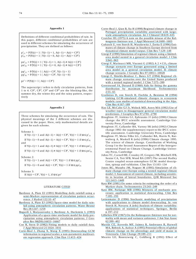
Definitions of different conditional probabilities of rain. Inthis paper, different conditional probabilities of rain areused in different schemes for simulating the occurrence ofprecipitation. They are defined as follows:

pi11 = P{Y(t) = 1 | Y(t–1) = 1, A(t–1) = A(t) = CPi}

pi01 = P{Y(t) = 1 | Y(t–1) = 0, A(t–1) = A(t) = CPi}

pni11 = P{Y(t) = 1 | Y(t–1) = 1, A(t–1) ≠ A(t) = CPi}

pni01 = P{Y(t) = 1 | Y(t–1) = 0, A(t–1) ≠ A(t) = CPi}

ppi11 = P{Y(t) = 1 | A(t) = CPi, Y(t–1) = 1}

ppi01 = P{Y(t) = 1 | A(t) = CPi, Y(t–1) = 0}

pri = P{Y(t) = 1 | A(t) = CPi}

The superscript i refers to daily circulation patterns, from1 to 4. CP1, CP2, CP3 and CP4 are the blocking-like, thesummer dry, the winter dry and the rainy pattern, respec-tively

Appendix 1

Three schemes for simulating the occurrence of rain. Thephysical meanings of the 3 different schemes are dis-cussed in the paper. Here, only mathematical details aregiven for each scheme.

Scheme 1: If Y(t–1) = 1 and A(t–1) = A(t) = CPi, Y(t) = 1 if ω ≤ pi

11

If Y(t–1) = 0 and A(t–1) = A(t) = CPi, Y(t) = 1 if ω ≤ pi01

andIf Y(t–1) = 1 and A(t–1) ≠ A(t) = CPi, Y(t) = 1 if ω ≤ pni

11

If Y(t–1) = 0 and A(t–1) ≠ A(t) = CPi, Y(t) = 1 if ω ≤ pni01

Scheme 2:If Y(t–1) = 1 and A(t) = CPi, Y(t) = 1 if ω ≤ ppi

11

If Y(t–1) = 0 and A(t) = CPi, Y(t) = 1 if ω ≤ ppi01

Scheme 3:If A(t) = CPi, Y(t) = 1, if ω ≤ pri

Appendix 2

Corte-Real et al.: A weather generator for daily precipitation scenarios

changes in interannual variability on CERES-wheatyields: sensitivity and 2 × CO2 general circulation modelstudies. Agric For Meteorol 62:159–189

Schubert S (1994) A weather generator based on the Euro-pean ‘Grosswetterlagen’. Clim Res 4:191–202

Schubert S, Henderson-Sellers A (1997) A statistical model todownscale local daily temperature extremes from synop-tic-scale atmospheric circulation patterns in the Australianregion. Clim Dyn 13:223–234

Semenov MA, Porter JR (1995) Climatic variability and themodelling of crop yields. Agric For Meteorol 73:265–283

Semenov MA, Brooks RJ, Barrow EM, Richardson CW (1998)Comparison of the WGEN and LARS-WG stochasticweather generators for diverse climate. Clim Res 10:95–107

Stern D, Coe R (1984) A model fitting analysis of daily rainfalldata (with discussion). J R Stat Soc Ser A 147:1–34

von Storch H, Zorita E, Cubasch U (1993) Downscaling ofglobal climate change estimates to regional scales: anapplication to Iberian rainfall in wintertime. J Clim6:1161–1171

Watson RT, Zinyowera MC, Moss RH (eds) (1996) Climatechange 1995: impacts, adaptations and mitigation of cli-mate change: scientific-technical analyses. Contributionof Working Group II to the Second Assessment Report ofIntergovernmental Panel on Climate Change. CambridgeUniversity Press, Cambridge

Wilks DS (1992) Adapting stochastic weather generationalgorithms for climate change studies. Clim Change22:67–84

Wilks DS (1995) Statistical methods in the atmospheric sci-ences: an introduction. Academic Press, San Diego

Wilson LL, Lettenmaier DP, Wood EF (1991) Simulation ofdaily precipitation in the Pacific Northwest using aweather classification scheme. Sur Geophys 12:127–142

Wilson LL, Lettenmaier DP, Skyllingstad E (1992) A hierarchi-cal stochastic model of large scale atmospheric circulationpatterns and multiple station daily precipitation. J Geo-phys Res 97:2791–2809

Zhang X, Wang XL, Corte-Real J (1997) On the relationshipsbetween daily circulation patterns and precipitation inPortugal. J Geophys Res 102:13495–13507

75

Editorial responsibility: Hans von Storch, Geesthacht, Germany

Submitted: July 30, 1998; Accepted: May 10, 1999Proofs received from author(s): August 5, 1999