
Simple, regular, and efficient numerical integration of rotational motion
25
The Astronomical Journal, 135:2298–2322, 2008 June doi:10.1088/0004-6256/135/6/2298 c 2008. The American Astronomical Society. All rights reserved. Printed in the U.S.A. SIMPLE, REGULAR, AND EFFICIENT NUMERICAL INTEGRATION OF ROTATIONAL MOTION Toshio Fukushima National Astronomical Observatory, Ohsawa, Mitaka, Tokyo 181-8588, Japan; [email protected] Received 2008 February 4; accepted 2008 March 12; published 2008 May 14 ABSTRACT Among various formulations to integrate rotational motions numerically, we recommend the integration of the combination of Euler parameters and the angular velocity components referred to the body-fixed reference frame with the renormalization of the Euler parameters at every integration step. This is because the formulation proposed is not only simple and regular, but also stable and precise in studying rotational motions numerically. Its efficiency is not degraded even for almost uniform rotations if their nominal uniform part is separated by Encke’s method. Key words: celestial mechanics – methods: numerical 1. INTRODUCTION Orbital and rotational dynamics are two major branches of classical mechanics (Goldstein et al. 2002). Therefore, it is natural to presume that both fields have been intensely studied in a similar manner. Of course, there are a number of analytical treatments of rotational motions. The classic standard textbooks are MacMillan (1936) and Whittaker (1947). In astronomy also, this is true, especially in discussing the Earth’s rotation. The latest reviews on this interesting and important topic are found in the reports of the IAU Division I Working Groups on nutation (Dehant et al. 1999) and on precession and ecliptic (Hilton et al. 2006), respectively. However, numerical researches are less prevalent in rotational dynamics. Why is this? The answer is probably because a simple, robust, and yet efficient formulation is not well established to integrate rota- tional motions numerically, such as the integration of rectangu- lar components of the physical position and velocity vectors in an inertial coordinate system in the case of orbital motions. A difficult issue is the proper choice of the kinematical variables to describe the orientation of a rotating body (Hughes 1986). One may argue that the well-known 3-1-3 Euler angles, as illus- trated on the front cover and in Figures 4–6 of Goldstein (1980) and geometrically defined below in Figure 12 in Appendix A.2, are sufficient for that purpose. In fact, this option has been adopted in practical studies of the rotational motion of the Moon (Cappallo et al. 1981) and of the Earth (Krasinsky 2006). Nevertheless, they become ill-determined when the magni- tude of the second angle is tiny (Fukushima 2003a). We will present an example in Section 2.1. This ill-determinacy of the 3-1-3 Euler angles significantly degrades the quality of numer- ical integrations of rotational motions, as will be illustrated in Section 2.2. On the other hand, numerical integration errors can induce qualitative changes of the integrated rotation such as a shift between the libration and circulation modes, which casts serious doubts on the reliability of numerical simulations. An example of this will be given in Section 2.3. Frequently it has been advocated that this type of difficulty can be bypassed by adopting a different combination of Euler angles such as the 1-2-3 convention, which is defined in Appendix A.3 and geometrically illustrated in Figure 12, or other similar combinations as usually chosen in aerodynamics and studies of attitude dynamics of space vehicles. However, this is not always true. First, an inappropriate choice of the inertial coordinate system to be referred easily cancels out the benefits of such a choice. An example of this would be encountered when integrating the rotation of Uranus by using the 1-2-3 Euler angles in an ecliptic coordinate system, since Uranus’ spin axis is tilted around 90 ◦ . Second, even if a suitable coordinate system is selected, a similar difficulty is unavoidable for some combinations of the initial conditions and the principal moments of inertia, especially for a truly triaxial body with a significantly oblique rotation axis. Finally, even if a suitable coordinate system is selected and the combination of the initial conditions and the principal moments of inertia is adequate to avoid troublesome situations for torque-free rotation, a similar impasse can be produced by strong torques. In Section 2.4, we will give an illustration. This undesirable phenomenon happens because, in such cases, some Euler angles vary in a circulating or librating man- ner with a large amplitude, and as a result, the second Euler angle may cross over its singular point, mπ or (m +1/2)π , where m is an arbitrary integer. As Deprit (1994) clearly pointed out, neither Andoyer canonical variables based on the 3-1-3 Eu- ler angles (Kinoshita 1972) nor their modifications using the 1-2-3 convention (Fukushima 1993) can completely eliminate this problem, although the latter is much more robust than the former. In attitude control problems, the difficulty in maneuver- ing the orientation of a vehicle caused by this issue is called the “gimbal lock,” which gained prominence when the landing module of Apollo 11 encountered it in the process of docking to the command module. Mathematically speaking, the issue is resolved only by using redundant variables such as four Euler parameters or nine com- ponents of the direction cosine matrix (DCM) (Hughes 1986). Of course, this is well known from the time of Euler. As a con- sequence, there are a number of treatises on rotational dynamics using Euler parameters or their equivalents such as quarternions, Cayley–Klein parameters, or spinols (Goldstein et al. 2002). For detailed information, see Arribas et al. (2006) and Brum- berg and Ivanova (2007), and references therein. For example, Altman (1972) proposed a numerical formulation to integrate the combination of four-dimensional Euler parameters and three inertial components of the rotational angular momentum vector. Similar approaches are popular in computational graphics and modern treatises of attitude dynamics. From a numerical viewpoint, however, this redundancy is a possible source of integration errors and, much worse, of numerical instabilities. In fact, we find that Altman’s approach is, in some cases, less precise and less stable than integrating the standard combination of 3-1-3 Euler angles and three body-fixed 2298
Transcript of Simple, regular, and efficient numerical integration of rotational motion
The Astronomical Journal, 135:2298–2322, 2008 June doi:10.1088/0004-6256/135/6/2298c© 2008. The American Astronomical Society. All rights reserved. Printed in the U.S.A.
SIMPLE, REGULAR, AND EFFICIENT NUMERICAL INTEGRATION OF ROTATIONAL MOTION
Toshio FukushimaNational Astronomical Observatory, Ohsawa, Mitaka, Tokyo 181-8588, Japan; [email protected]
Received 2008 February 4; accepted 2008 March 12; published 2008 May 14
ABSTRACT
Among various formulations to integrate rotational motions numerically, we recommend the integration of thecombination of Euler parameters and the angular velocity components referred to the body-fixed reference framewith the renormalization of the Euler parameters at every integration step. This is because the formulation proposedis not only simple and regular, but also stable and precise in studying rotational motions numerically. Its efficiencyis not degraded even for almost uniform rotations if their nominal uniform part is separated by Encke’s method.
Key words: celestial mechanics – methods: numerical
1. INTRODUCTION
Orbital and rotational dynamics are two major branches ofclassical mechanics (Goldstein et al. 2002). Therefore, it isnatural to presume that both fields have been intensely studiedin a similar manner. Of course, there are a number of analyticaltreatments of rotational motions. The classic standard textbooksare MacMillan (1936) and Whittaker (1947). In astronomy also,this is true, especially in discussing the Earth’s rotation. Thelatest reviews on this interesting and important topic are foundin the reports of the IAU Division I Working Groups on nutation(Dehant et al. 1999) and on precession and ecliptic (Hiltonet al. 2006), respectively. However, numerical researches areless prevalent in rotational dynamics. Why is this?
The answer is probably because a simple, robust, and yetefficient formulation is not well established to integrate rota-tional motions numerically, such as the integration of rectangu-lar components of the physical position and velocity vectors inan inertial coordinate system in the case of orbital motions. Adifficult issue is the proper choice of the kinematical variablesto describe the orientation of a rotating body (Hughes 1986).One may argue that the well-known 3-1-3 Euler angles, as illus-trated on the front cover and in Figures 4–6 of Goldstein (1980)and geometrically defined below in Figure 12 in Appendix A.2,are sufficient for that purpose. In fact, this option has beenadopted in practical studies of the rotational motion of the Moon(Cappallo et al. 1981) and of the Earth (Krasinsky 2006).
Nevertheless, they become ill-determined when the magni-tude of the second angle is tiny (Fukushima 2003a). We willpresent an example in Section 2.1. This ill-determinacy of the3-1-3 Euler angles significantly degrades the quality of numer-ical integrations of rotational motions, as will be illustrated inSection 2.2. On the other hand, numerical integration errors caninduce qualitative changes of the integrated rotation such as ashift between the libration and circulation modes, which castsserious doubts on the reliability of numerical simulations. Anexample of this will be given in Section 2.3.
Frequently it has been advocated that this type of difficulty canbe bypassed by adopting a different combination of Euler anglessuch as the 1-2-3 convention, which is defined in Appendix A.3and geometrically illustrated in Figure 12, or other similarcombinations as usually chosen in aerodynamics and studiesof attitude dynamics of space vehicles. However, this is notalways true.
First, an inappropriate choice of the inertial coordinate systemto be referred easily cancels out the benefits of such a choice.
An example of this would be encountered when integrating therotation of Uranus by using the 1-2-3 Euler angles in an eclipticcoordinate system, since Uranus’ spin axis is tilted around90. Second, even if a suitable coordinate system is selected,a similar difficulty is unavoidable for some combinations ofthe initial conditions and the principal moments of inertia,especially for a truly triaxial body with a significantly obliquerotation axis. Finally, even if a suitable coordinate system isselected and the combination of the initial conditions and theprincipal moments of inertia is adequate to avoid troublesomesituations for torque-free rotation, a similar impasse can beproduced by strong torques. In Section 2.4, we will give anillustration.
This undesirable phenomenon happens because, in suchcases, some Euler angles vary in a circulating or librating man-ner with a large amplitude, and as a result, the second Euler anglemay cross over its singular point, mπ or (m + 1/2)π , where mis an arbitrary integer. As Deprit (1994) clearly pointed out,neither Andoyer canonical variables based on the 3-1-3 Eu-ler angles (Kinoshita 1972) nor their modifications using the1-2-3 convention (Fukushima 1993) can completely eliminatethis problem, although the latter is much more robust than theformer. In attitude control problems, the difficulty in maneuver-ing the orientation of a vehicle caused by this issue is calledthe “gimbal lock,” which gained prominence when the landingmodule of Apollo 11 encountered it in the process of dockingto the command module.
Mathematically speaking, the issue is resolved only by usingredundant variables such as four Euler parameters or nine com-ponents of the direction cosine matrix (DCM) (Hughes 1986).Of course, this is well known from the time of Euler. As a con-sequence, there are a number of treatises on rotational dynamicsusing Euler parameters or their equivalents such as quarternions,Cayley–Klein parameters, or spinols (Goldstein et al. 2002).For detailed information, see Arribas et al. (2006) and Brum-berg and Ivanova (2007), and references therein. For example,Altman (1972) proposed a numerical formulation to integratethe combination of four-dimensional Euler parameters and threeinertial components of the rotational angular momentum vector.Similar approaches are popular in computational graphics andmodern treatises of attitude dynamics.
From a numerical viewpoint, however, this redundancy isa possible source of integration errors and, much worse, ofnumerical instabilities. In fact, we find that Altman’s approachis, in some cases, less precise and less stable than integrating thestandard combination of 3-1-3 Euler angles and three body-fixed
2298
No. 6, 2008 NUMERICAL INTEGRATION OF ROTATIONAL MOTION 2299
-180
-150
-120
-90
-60
-30
0
30
0 0.5 1 1.5 2
ψ (
deg)
Time/Period
Euler Angle Variation: ψ
ωA0 /ωC=10−6, ωB0=ψ0=φ0=0θ0=−1"
−0.5"
−0.2"
−0.1"
−0.02"
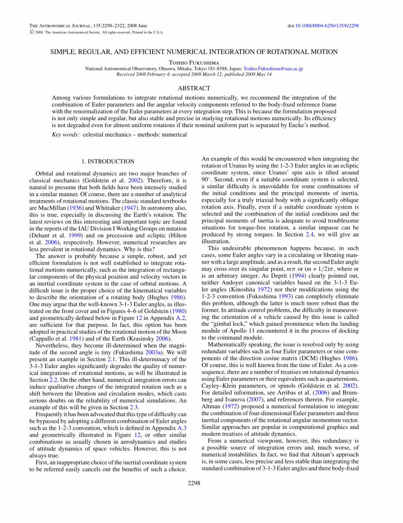
Figure 1. Peculiar variation of the precession angle. Shown are the timevariations of ψ , the first Euler angle in the 3-1-3 convention for the case oftorque-free rotation of a spheroidal rigid body. The time is measured in units ofthe nominal rotation period, 2π/ωC0. In this case, ωC is a constant of motionsince the rotating body is spherically symmetric. The ratios of the principalmoments of inertia are chosen in order to approximate the actual Earth suchthat (C − A)/C = (C − B)/C = 3.28 × 10⁻³. The initial conditions ofthe Euler angles are set as ψ0 = φ0 = 0, while θ0 is changed as shown inthe figure. The smallness of |ψ0| and |θ0| indicates that the adopted referenceframe is quite close to an equatorial coordinate system at the initial epoch. Theinitial conditions of the body-fixed angular velocity components are taken asωA0/ωC0 = 10−6 and ωB0 = 0 in order to mimic the actual polar motion of theEarth, the magnitude of which is of the order of 0.1′′. When |θ0| is sufficientlysmall, the curve of ψ resembles a zigzag pattern despite the fact that the motionitself remains regular, as described in the text.
components of the angular velocity vector. See the example inSection 2.5.
Judging from the current circumstances as reviewed above,we should say that no all-purpose treatise in studying rotationalmotions numerically has so far been established. In order toovercome this situation, we (1) conduct an extensive surveyof possible combinations of the kinematical and dynamicalvariables, summarized in Appendix A, (2) examine their costand performance in numerical simulations of rotational motionsin Section 5, (3) confirm that performing the renormalization ofEuler parameters and/or their orthogonalization with their timederivatives at every integration step, which will be described inSection 3, significantly stabilizes their numerical integrations,and (4) find that the pair of Euler parameters and the body-fixedcomponents of the angular velocity vector with the applicationof the above renormalization is the most efficient combination ofvariables in the sense that its numerical integration runs fastestand produces fewest integration errors.
In dealing with an almost uniform rotation, however, theeffectiveness of the formulations using Euler parameters isdiminished and those based on a certain combination of Eulerangles become more efficient. In such cases, we apply Encke’smethod to the formulations using Euler parameters in order toseparate the part of nominal uniform rotation, which will beintroduced in Section 4. This restores the superiority of themethod using Euler parameters with renormalization.
2. EXAMPLES OF INAPPROPRIATE FORMULATIONS
2.1. Vulnerability of Euler Angles
Let us illustrate some examples where existing numericalformulations fail to simulate rotational motions precisely. First,we consider a simple case: the rotation of a spheroidal butnearly spherical rigid body under no torque. Also we set themagnitude of the initial polar motion, which is the angle between
-1.4
-1.2
-1
-0.8
-0.6
-0.4
-0.2
0
0 0.5 1 1.5 2
θ(")
Time/Period
Euler Angle Variation: θ
ωA0 /ωC=10−6, ωB0=ψ0=φ0=0
θ0=−0.02" −0.1"−0.2"
−0.5"
−1"
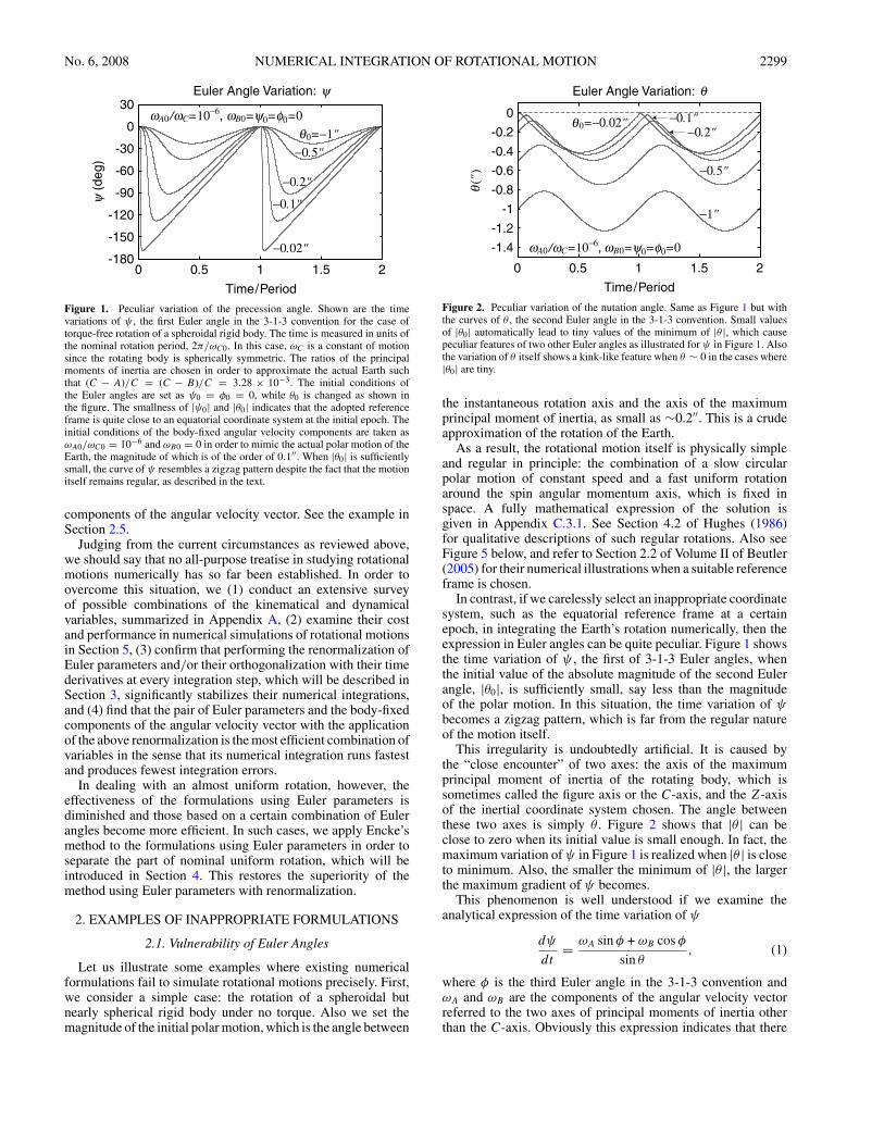
Figure 2. Peculiar variation of the nutation angle. Same as Figure 1 but withthe curves of θ , the second Euler angle in the 3-1-3 convention. Small valuesof |θ0| automatically lead to tiny values of the minimum of |θ |, which causepeculiar features of two other Euler angles as illustrated for ψ in Figure 1. Alsothe variation of θ itself shows a kink-like feature when θ ∼ 0 in the cases where|θ0| are tiny.
the instantaneous rotation axis and the axis of the maximumprincipal moment of inertia, as small as ∼0.2′′. This is a crudeapproximation of the rotation of the Earth.
As a result, the rotational motion itself is physically simpleand regular in principle: the combination of a slow circularpolar motion of constant speed and a fast uniform rotationaround the spin angular momentum axis, which is fixed inspace. A fully mathematical expression of the solution isgiven in Appendix C.3.1. See Section 4.2 of Hughes (1986)for qualitative descriptions of such regular rotations. Also seeFigure 5 below, and refer to Section 2.2 of Volume II of Beutler(2005) for their numerical illustrations when a suitable referenceframe is chosen.
In contrast, if we carelessly select an inappropriate coordinatesystem, such as the equatorial reference frame at a certainepoch, in integrating the Earth’s rotation numerically, then theexpression in Euler angles can be quite peculiar. Figure 1 showsthe time variation of ψ , the first of 3-1-3 Euler angles, whenthe initial value of the absolute magnitude of the second Eulerangle, |θ0|, is sufficiently small, say less than the magnitudeof the polar motion. In this situation, the time variation of ψbecomes a zigzag pattern, which is far from the regular natureof the motion itself.
This irregularity is undoubtedly artificial. It is caused bythe “close encounter” of two axes: the axis of the maximumprincipal moment of inertia of the rotating body, which issometimes called the figure axis or the C-axis, and the Z-axisof the inertial coordinate system chosen. The angle betweenthese two axes is simply θ . Figure 2 shows that |θ | can beclose to zero when its initial value is small enough. In fact, themaximum variation of ψ in Figure 1 is realized when |θ | is closeto minimum. Also, the smaller the minimum of |θ |, the largerthe maximum gradient of ψ becomes.
This phenomenon is well understood if we examine theanalytical expression of the time variation of ψ
dψ
dt= ωA sin φ + ωB cos φ
sin θ, (1)
where φ is the third Euler angle in the 3-1-3 convention andωA and ωB are the components of the angular velocity vectorreferred to the two axes of principal moments of inertia otherthan the C-axis. Obviously this expression indicates that there

2300 FUKUSHIMA Vol. 135
-15-14-13-12-11-10
-9-8-7-6-5
0 1 2 3 4 5 6 7 8
log 1
0|∆ R
|
Time/Period
Integration Error Variation
RK4, 1024 Steps/PeriodωA0 /ωC=10−6, ωB0=ψ0=φ0=0
θ0=−0.01"
−0.02"
−0.05"
−0.1"
Figure 3. Integration errors of torque-free rotation in an inappropriatecoordinate system. Same as Figure 1 but with the variations of the logarithmof the total error of the coordinate triad R. The time evolution of the triad isobtained by numerical integration of the 3-1-3 Euler angles and the body-fixedcomponents of the angular velocity, (ψ, θ, φ, ωA, ωB, ωC ). The errors shownare measured by comparing with the analytical solution. When |θ0| is small, sayless than or equal to −0.05′′, the errors behave like step functions. The changein the errors occurs when |θ | ≈ 0, namely at the timings of the so-called “closeencounter” of the figure axis and the Z-axis of the adopted coordinate system.
exist singularities of the form sin θ = 0, i.e. θ = mπ , where mis an arbitrary integer.
2.2. Integration Errors and Close Encounter
In principle, this issue on the peculiar behavior of Eulerangles produces no practical difficulties provided their analyticalsolutions are obtained in a closed form, such as for the torque-free rotation of a rigid body. However, the story becomescompletely different if we evaluate them through numericalintegrations. Most numerical integrators are designed to followregular and smooth motions, which are well expressed by low-order time polynomials. Therefore, numerical integrations ofthese Euler angles suffer loss of precision or instabilities whenthey vary violently, as shown in Figure 1.
Figure 3 illustrates the numerical integration errors of thesame rotation as described in Figures 1 and 2. The integratorused is the fourth-order Runge–Kutta method of a fixed step size,∆t , which is taken sufficiently small as 1/1024 of the nominalrotation period, 2π/ωC . More specifically, we plot the variationsof the logarithm of the total error of the coordinate triad,
|∆R| ≡√
|∆eA|2 + |∆eB |2 + |∆eC |2, (2)
where ∆eJ denotes the error of eJ , the J th base vector express-ing the body-fixed coordinate system. The time evolution of thetriad is obtained by numerical integrations of the 3-1-3 Eulerangles and the body-fixed components of the angular veloc-ity, (ψ, θ, φ, ωA, ωB, ωC). The errors shown are measured bycomparing with the analytical solution.
It is interesting to see that the errors behave like step functionsif |θ0| is sufficiently small, say less than or equal to 0.05′′. Theerror jump occurs when |θ | ≈ 0, namely at the timings of theso-called “close encounter” of the figure axis and the Z-axisof the adopted coordinate system. See Section 2 of Fukushima(2003a), where we encountered similar difficulties in improvingprecession formulae.
2.3. Mode Change due to Integration Errors
Even if |θ0| is not small, odd situations occur when theprecision of numerical integration is low. Figure 4 illustrates
-15000
-10000
-5000
0
5000
10000
15000
20000
0 5 10 15 20 25 30 35 40 45 50
ψ (
deg)
Time/Period
Euler Angle Variation: ψ
ωA0 /ωC=10−6, ωB0=ψ0=φ0=0, θ0=−0.01"
RK4Steps/Period=128
25664
16
True
Figure 4. Result of low-precision integrations. Same as Figure 1 for the caseθ0 = −0.01′′, but with the results obtained by numerical integration with variousstep sizes as shown. The integrator used is the fourth-order Runge–Kutta methodwith a constant step size. The true solution is a periodic motion oscillating around−90.
the precision dependence of the integrated ψ . The true solutionis the repetition of the zigzag pattern already shown in Figure 1.In depicting the figure, we fixed the integrator to be the same asin Figure 3 while changing the step size, ∆t , from 1/16, 1/64,1/128, to 1/256 of the nominal rotation period, P . We omit theresult of the case 1/32, which is almost the same as that of 1/64.Also if the step size is smaller than 1/512 of the period, thedifferences from the true solution are too small to be seen in thefigure.
Figure 4 clearly indicates that integration errors can changethe nature of numerical solutions drastically, from the librationmode to the circulation mode in this case. Also the lower theprecision, the more frequently the change of modes occurs. Thisvulnerability becomes troublesome in extracting meaningfulresults from simulations.
2.4. Mode Change due to Strong Torque
Of course, an appropriate choice of the inertial coordinatesystem can avoid the difficulty seen in the previous subsections.Figure 5 shows the torque-free rotation of a truly triaxial rigidbody, the asteroid Ida, in a suitably chosen inertial coordinatesystem. Ida is far from spherical and/or oblately spheroidalbecause its ratios of the principal moments of inertia areA/C = 0.234,80 and B/C = 0.929,12. Rather, the asteroidis close to being prolately spheroidal. Illustrated in the figureare the analytical solution curves of the 3-1-3 Euler angles and ofthe Euler parameters, (q0, q1, q2, q3). In the figure, we removedthe secular part of the rotation angle, φ. Also we added suitableoffsets to the curves of the variables except θ in order to avoidthem overlapping with each other.
The initial condition is chosen such that (1) the rotationalperiod is the same as the observed period of Ida, i.e. around4.6 h, (2) the initial rotation axis is inclined around 5 to the C-axis, and (3) the inertial coordinate system is selected such thatthe Z-axis is inclined around 23.5 to the initial C-axis. The lastcondition is in order to avoid the so-called “close encounter”of the Z-axis and the C-axis during the rotation. As a result,the time evolution of the 3-1-3 Euler angles is regular, as arethe Euler parameters in Figure 5. This is because the variationof θ is not as large as −32.3 < θ < −14.6, such that theclose encounter can be avoided eternally by setting the Z-axissufficiently far from the initial C-axis.
No. 6, 2008 NUMERICAL INTEGRATION OF ROTATIONAL MOTION 2301
-16-14-12-10
-8-6-4-2024
0 1 2 3 4 5 6 7 8 9
Var
iabl
es
Time/Period
Torque-Free Rotation: Ida
ψ
θφq0
q1
q2
q3
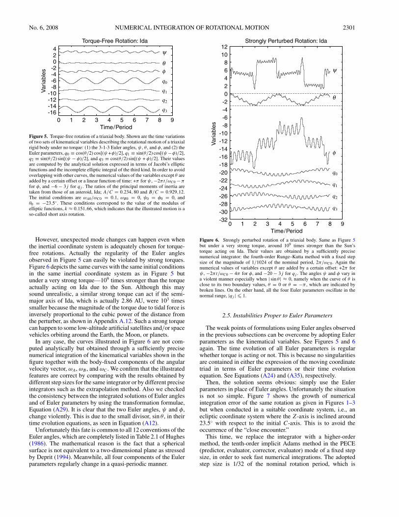
Figure 5. Torque-free rotation of a triaxial body. Shown are the time variationsof two sets of kinematical variables describing the rotational motion of a triaxialrigid body under no torque: (1) the 3-1-3 Euler angles, ψ , θ , and φ, and (2) theEuler parameters, q0 ≡ cos(θ/2) cos[(ψ +φ)/2], q1 ≡ sin(θ/2) cos[(ψ −φ)/2],q2 ≡ sin(θ/2) sin[(ψ − φ)/2], and q3 ≡ cos(θ/2) sin[(ψ + φ)/2]. Their valuesare computed by the analytical solution expressed in terms of Jacobi’s ellipticfunctions and the incomplete elliptic integral of the third kind. In order to avoidoverlapping with other curves, the numerical values of the variables except θ areadded by a certain offset or a linear function of time: +π for ψ , −2πt/ωC0 − π
for φ, and −6 − 3j for qj . The ratios of the principal moments of inertia aretaken from those of an asteroid, Ida; A/C = 0.234, 80 and B/C = 0.929,12.The initial conditions are ωA0/ωC0 = 0.1, ωB0 = 0, ψ0 = φ0 = 0, andθ0 = −23.5. These conditions correspond to the value of the modulus ofelliptic functions, k ≈ 0.151,66, which indicates that the illustrated motion is aso-called short axis rotation.
However, unexpected mode changes can happen even whenthe inertial coordinate system is adequately chosen for torque-free rotations. Actually the regularity of the Euler anglesobserved in Figure 5 can easily be violated by strong torques.Figure 6 depicts the same curves with the same initial conditionsin the same inertial coordinate system as in Figure 5 butunder a very strong torque—109 times stronger than the torqueactually acting on Ida due to the Sun. Although this maysound unrealistic, a similar strong torque can act if the semi-major axis of Ida, which is actually 2.86 AU, were 103 timessmaller because the magnitude of the torque due to tidal force isinversely proportional to the cubic power of the distance fromthe perturber, as shown in Appendix A.12. Such a strong torquecan happen to some low-altitude artificial satellites and/or spacevehicles orbiting around the Earth, the Moon, or planets.
In any case, the curves illustrated in Figure 6 are not com-puted analytically but obtained through a sufficiently precisenumerical integration of the kinematical variables shown in thefigure together with the body-fixed components of the angularvelocity vector, ωA, ωB , and ωC . We confirm that the illustratedfeatures are correct by comparing with the results obtained bydifferent step sizes for the same integrator or by different preciseintegrators such as the extrapolation method. Also we checkedthe consistency between the integrated solutions of Euler anglesand of Euler parameters by using the transformation formulae,Equation (A29). It is clear that the two Euler angles, ψ and φ,change violently. This is due to the small divisor, sin θ , in theirtime evolution equations, as seen in Equation (A12).
Unfortunately this fate is common to all 12 conventions of theEuler angles, which are completely listed in Table 2.1 of Hughes(1986). The mathematical reason is the fact that a sphericalsurface is not equivalent to a two-dimensional plane as stressedby Deprit (1994). Meanwhile, all four components of the Eulerparameters regularly change in a quasi-periodic manner.
-32-30-28-26-24-22-20-18-16-14-12-10-8-6-4-202468
1012
0 1 2 3 4 5 6 7 8 9
Var
iabl
es
Time/Period
Strongly Perturbed Rotation: Ida
ψ
θ
φ
q0
q1
q2
q3
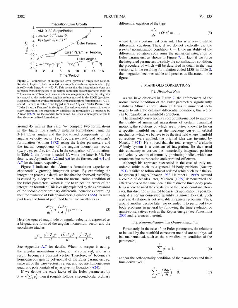
Figure 6. Strongly perturbed rotation of a triaxial body. Same as Figure 5but under a very strong torque, around 109 times stronger than the Sun’storque acting on Ida. Their values are obtained by a sufficiently precisenumerical integrator: the fourth-order Runge–Kutta method with a fixed stepsize of the magnitude of 1/1024 of the nominal period, 2π/ωC0. Again thenumerical values of variables except θ are added by a certain offset: +2π forψ , −2πt/ωC0 − 4π for φ, and −20 − 3j for qj . The angles ψ and φ vary ina violent manner especially when | sin θ | ≈ 0, namely when the curve of θ isclose to its two boundary values, θ = 0 or θ = −π , which are indicated bybroken lines. On the other hand, all the four Euler parameters oscillate in thenormal range, |qj | 1.
2.5. Instabilities Proper to Euler Parameters
The weak points of formulations using Euler angles observedin the previous subsections can be overcome by adopting Eulerparameters as the kinematical variables. See Figures 5 and 6again. The time evolution of all Euler parameters is regularwhether torque is acting or not. This is because no singularitiesare contained in either the expression of the moving coordinatetriad in terms of Euler parameters or their time evolutionequation. See Equations (A24) and (A35), respectively.
Then, the solution seems obvious: simply use the Eulerparameters in place of Euler angles. Unfortunately the situationis not so simple. Figure 7 shows the growth of numericalintegration error of the same rotation as given in Figures 1–3but when conducted in a suitable coordinate system, i.e., anecliptic coordinate system where the Z-axis is inclined around23.5 with respect to the initial C-axis. This is to avoid theoccurrence of the “close encounter.”
This time, we replace the integrator with a higher-ordermethod, the tenth-order implicit Adams method in the PECE(predictor, evaluator, corrector, evaluator) mode of a fixed stepsize, in order to seek fast numerical integrations. The adoptedstep size is 1/32 of the nominal rotation period, which is
2302 FUKUSHIMA Vol. 135
-16-14-12-10-8-6-4-202
0 2 4 6 8 10 12 14 16
log 1
0|∆R
|
Time/Period
Integration Error Growth
AM10, 32 Steps/PeriodωA0 /ωC=10−6, ωB0=0ψ0=φ0=0, θ0=−23.5o
Euler Param.
Euler Param. + Renorm.
Euler Angles
Figure 7. Comparison of integration error growth of torque-free rotation.Similar to Figure 3, but conducted in a suitable coordinate system where |θ0|is sufficiently large, θ0 = −23.5. This means that the integration is done in areference frame being close to the ecliptic coordinate system in order to avoid the“close encounter.” In order to seek an efficient integration scheme, the integratoris changed to the tenth-order implicit Adams method in the PECE (predictor,evaluator, corrector, evaluator) mode. Compared are three formulations: 1A, 3B,and M3B coded in Table 2 and tagged as “Euler Angles,” “Euler Param.,” and“Euler Param. + Renorm.” in the figure. The enforcement of renormalization atevery integration step successfully stabilizes the formulation 3B proposed byAltman (1972). Yet the standard formulation, 1A, leads to more precise resultsthan the renormalized formulation.
around 45 min in this case. We compare two formulationsin the figure: the standard Eulerian formulation using the3-1-3 Euler angles and the body-fixed components of theangular velocity vector, (ψ, θ, φ, ωA, ωB, ωC), and Altman’sformulation (Altman 1972) using the Euler parameters andthe inertial components of the angular momentum vector,(q0, q1, q2, q3, LX,LY , LZ). In the comparison of formulationsin Table 2, the former is coded 1A while the latter is 3B. Fordetails, see Appendices A.2 and A.6 for the former, and A.4 andA.7 for the latter, respectively.
Figure 7 indicates that Altman’s formulation experiencesexponentially growing integration errors. By examining theintegration process in detail, we find that the observed instabilityis caused by a departure from the normalization condition ofthe Euler parameters, which is due to truncation errors of theintegration formulae. This is easily explained by the expressionsof the second-order ordinary differential equations controllingthe time evolution of Euler parameters, Equation (A56). Its mainpart takes the form of perturbed harmonic oscillators as
d2qj
dt2 +
(ω2
4
)qj = · · · . (3)
Here the squared magnitude of angular velocity is expressed asa bi-quadratic form of the angular momentum vector and thecoordinate triad as
ω2 = ( L · eA)2
A2+
( L · eB)2
B2+
( L · eC)2
C2. (4)
See Appendix A.7 for details. When no torque is acting,the angular momentum vector, L, is conserved, and as aresult, becomes a constant vector. Therefore, ω2 becomes ahomogeneous quartic polynomial of the Euler parameters, qj ,since all of the base vectors, eA, eB , and eC , are homogeneousquadratic polynomials of qj as given in Equation (A24).
If we denote the scale factor of the Euler parameters byλ ≡
√∑j q2
j , then it roughly follows a second-order ordinary
differential equation of the type
d2λ
dt2 + Ω2λ5 = · · · , (5)
where Ω is a certain real constant. This is a very unstabledifferential equation. Thus, if we do not explicitly use thea priori normalization condition, λ = 1, the instability of thedifferential equation soon ruins the numerical integration ofEuler parameters, as shown in Figure 7. In fact, if we forcethe integrated parameters to satisfy the normalization condition,the procedure of which will be described in detail in the nextsection with the resulting formulation coded M3B in Table 2,the integration becomes stable and precise, as illustrated in thefigure.
3. MANIFOLD CORRECTIONS
3.1. Historical Note
As we have observed in Figure 7, the enforcement of thenormalization condition of the Euler parameters significantlystabilizes Altman’s formulation. In terms of numerical tech-niques to integrate ordinary differential equations, this recipecan be regarded as a manifold correction.
The manifold correction is a sort of meta-method to improvethe quality of numerical integrations of certain dynamicalmotions, the solutions of which are a priori known to lie ona specific manifold such as the isoenergy curve. In orbitalmechanics, which we believe to be the first field where manifoldcorrections were applied, the original idea was invented byNacozy (1971). He noticed that the total energy of a classicN -body system is a constant of integration. He then usedthis constancy to correct the numerically integrated positionand velocity vectors of mutually gravitating bodies, which areerroneous due to truncation and/or round-off errors.
Although his approach succeeded in the case of truly un-ordered orbits such as a general 25-body problem (Nacozy1971), it failed to follow almost ordered orbits such as in the so-lar system (Huang & Innanen 1983; Hairer et al. 1999). Arounda couple of decades later, Murison (1989) demonstrated theeffectiveness of the same idea in the restricted three-body prob-lems where he used the constancy of the Jacobi constant. How-ever, this direction is limited because its application is possibleonly if a certain conserved quantity is known to exist. Sucha physical relation is not available in general problems. Thus,around another decade later, we extended it to perturbed two-body problems in general by following the time evolution ofquasi-conservatives such as the Kepler energy (see Fukushima2005 and references therein).
3.2. Renormalization and Orthogonalization
Fortunately, in the case of the Euler parameters, the relationsto be used by the manifold correction method are not physicalbut mathematical, such as the normalization condition of theparameters,
3∑i=0
q2i = 1, (6)
and/or the orthogonality condition of the parameters and theirtime derivatives,
3∑i=0
qi
(dqi
dt
)= 0. (7)
No. 6, 2008 NUMERICAL INTEGRATION OF ROTATIONAL MOTION 2303
When the Euler parameters are adopted as the integratedvariables, the former condition is available. If, further, theirtime derivatives are also to be integrated, both relations can beused. In any case, their availability is always assured.
As for the actual correction procedure, we adopt the scalingmethod, as was done in Fukushima (2003b), when only thenormalization condition is available,
qj → qj ≡ qj√∑3i=0 q2
i
(8)
where the index j runs from 0 to 3. This may be called therenormalization. On the other hand, if both the normalizationand orthogonality conditions can be used, we first apply theabove renormalization procedure and then remove the non-orthogonal part from the derivative side only as
dqj
dt→
(dqj
dt
)≡ dqj
dt−
[3∑
i=0
qi
(dqi
dt
)]qj , (9)
for j = 0, 1, 2, 3. This operation is a kind of rotation of the timederivatives, dqj/dt , in the artificial four-dimensional space ofthe Euler parameters. The situation is similar to the case weexperienced in treating the orthogonality of the orbital angularmomentum and Laplace vector in real three-dimensional space(Fukushima 2003c).
3.3. Timing of Manifold Corrections
From the viewpoint of constructing numerical integrators,manifold corrections can be regarded as kinds of correctorswithout using function evaluations in general. Therefore, theireffects depend on the timing of when the corrections are con-ducted during the numerical integration procedure. Experiencetells us that the best timing is immediately after the Euler pa-rameters and/or their time derivatives are estimated.
For example, the integration procedure of the fourth-orderRunge–Kutta method is symbolically expressed as
P1/2E1/2C1/2E1/2P1E1C1E1,
where P, E, and C stand for the predictor, evaluator, andcorrector, respectively. The subscript is the step index, wherethe index 1 corresponds to the next step and fractional indicescorrespond to internal points. The actual form of P or C maydiffer if the index is different.
We put the manifold corrector, M, immediately after P or Cin this case. The resulting symbolic description is
P1/2M1/2E1/2C1/2M1/2E1/2P1M1E1C1M1E1.
Similarly, the application of manifold correction to the Adamsmethod becomes
P1M1E1
for the PE mode,P1M1E1C1M1
for the PEC mode, and
P1M1E1C1M1E1
for the PECE mode, respectively.
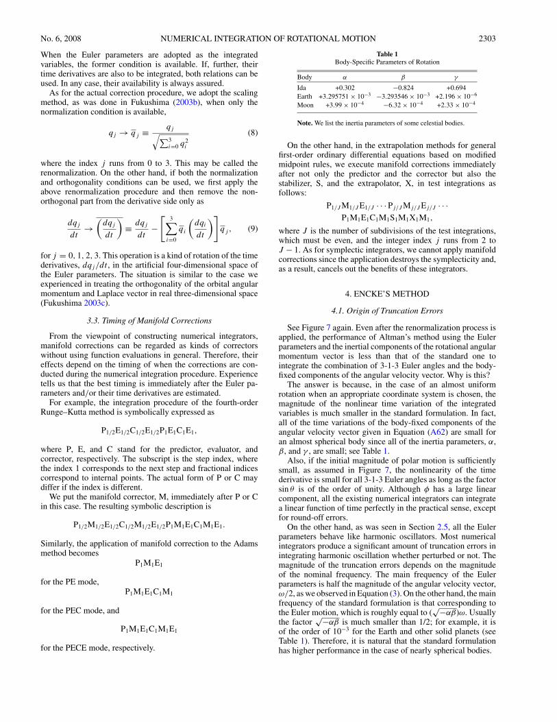
Table 1Body-Specific Parameters of Rotation
Body α β γ
Ida +0.302 −0.824 +0.694Earth +3.295751 × 10⁻³ −3.293546 × 10⁻³ +2.196 × 10⁻⁶
Moon +3.99 × 10⁻⁴ −6.32 × 10⁻⁴ +2.33 × 10⁻⁴
Note. We list the inertia parameters of some celestial bodies.
On the other hand, in the extrapolation methods for generalfirst-order ordinary differential equations based on modifiedmidpoint rules, we execute manifold corrections immediatelyafter not only the predictor and the corrector but also thestabilizer, S, and the extrapolator, X, in test integrations asfollows:
P1/J M1/J E1/J · · · Pj/J Mj/J Ej/J · · ·P1M1E1C1M1S1M1X1M1,
where J is the number of subdivisions of the test integrations,which must be even, and the integer index j runs from 2 toJ − 1. As for symplectic integrators, we cannot apply manifoldcorrections since the application destroys the symplecticity and,as a result, cancels out the benefits of these integrators.
4. ENCKE’S METHOD
4.1. Origin of Truncation Errors
See Figure 7 again. Even after the renormalization process isapplied, the performance of Altman’s method using the Eulerparameters and the inertial components of the rotational angularmomentum vector is less than that of the standard one tointegrate the combination of 3-1-3 Euler angles and the body-fixed components of the angular velocity vector. Why is this?
The answer is because, in the case of an almost uniformrotation when an appropriate coordinate system is chosen, themagnitude of the nonlinear time variation of the integratedvariables is much smaller in the standard formulation. In fact,all of the time variations of the body-fixed components of theangular velocity vector given in Equation (A62) are small foran almost spherical body since all of the inertia parameters, α,β, and γ , are small; see Table 1.
Also, if the initial magnitude of polar motion is sufficientlysmall, as assumed in Figure 7, the nonlinearity of the timederivative is small for all 3-1-3 Euler angles as long as the factorsin θ is of the order of unity. Although φ has a large linearcomponent, all the existing numerical integrators can integratea linear function of time perfectly in the practical sense, exceptfor round-off errors.
On the other hand, as was seen in Section 2.5, all the Eulerparameters behave like harmonic oscillators. Most numericalintegrators produce a significant amount of truncation errors inintegrating harmonic oscillation whether perturbed or not. Themagnitude of the truncation errors depends on the magnitudeof the nominal frequency. The main frequency of the Eulerparameters is half the magnitude of the angular velocity vector,ω/2, as we observed in Equation (3). On the other hand, the mainfrequency of the standard formulation is that corresponding tothe Euler motion, which is roughly equal to (
√−αβ)ω. Usuallythe factor
√−αβ is much smaller than 1/2; for example, it isof the order of 10−3 for the Earth and other solid planets (seeTable 1). Therefore, it is natural that the standard formulationhas higher performance in the case of nearly spherical bodies.
2304 FUKUSHIMA Vol. 135
4.2. Historical Note
The inferiority of formulations using Euler parameters seenin the previous subsection is due to the fact that the magnitudeof the main frequency is large. However, as will be seen below,this can be overcome if we analytically remove the uniform partbefore conducting numerical integrations. This is the core ideaof Encke’s method (Fukushima 1996).
The method itself was invented by Encke to follow thetime evolution of nearly parabolic orbits efficiently (Brouwer& Clemence 1961). As the new variables, he adopts thefinite difference in rectangular coordinates from the referencesolution, which he assumes to be an osculating Keplerian(usually parabolic) orbit initially. As a result, the right-handside of the equation of motion with respect to the new variablesis expressed as the difference of quantities of almost thesame magnitude, the direct evaluation of which gives rise toa loss of precision due to rounding. Encke cleverly avoids thissituation by rewriting the troublesome terms into a form directlyproportional to the small terms. This idea is not limited tothe numerical integration of cometary motion in rectangularcoordinates. In fact, we extended it to more general cases(Fukushima 1996).
4.3. Application of Encke’s Method to Almost Uniform Rotation
Let us apply Encke’s idea to an almost uniform rotation.As the reference solution, we adopt a uniform rotation whichis osculating initially, namely a rotation with constant angularvelocity vector the same as the initial value, ω0. In order tosimplify the problem, we adopt an inertial coordinate systemsuch that its Z-axis is parallel with ω0. Then, the referencesolution becomes a uniform rotation around the third axis withconstant speed of rotation, ω0 ≡ |ω0|. The correspondingrotation matrix is R3(−ω0t).
Taking this into account, we introduce an intermediate coor-dinate triad,
P ≡ (eD, eE, eC), (10)
such that the body-fixed coordinate triad is expressed as aproduct of P and the above uniform rotation as
R = P R3(−ω0t). (11)
In general, we can adopt another definition by reversing the orderof the matrix product as R = R3(−ω0t)P . However, we preferthe above form, Equation (11), since it resembles the standarddescription of the Earth’s rotation where P plays the role of theprecession–nutation matrix while R3(−ω0t) corresponds to thesidereal rotation.
Once the intermediate coordinate triad is introduced, thenthe remaining procedure to realize Encke’s method is trivial.In Appendix B, we give details of an application of Encke’smethod. In any case, the magnitude of the new main frequencybecomes small. For example, in the case of Encke’s methodapplied to Euler parameters it becomes |∆ ω|/2. Therefore, theintegration errors of the new variables are expected to diminishsignificantly. In fact, in the case of Euler parameters, their errorsreduce so greatly that the main error sources are not those inthe Euler parameters but those in the delta angular velocitycomponents, which are roughly of the same order as those ofthe standard formulation after Encke’s method is applied.
11.21.41.61.8
22.22.42.6
0 1 2 3 4 5 6 7 8
CP
U T
ime
Rat
io to
3A
Number of Perturbers
Comparison of CPU Times
1C
1A4A3B
1B4B
3C
4C
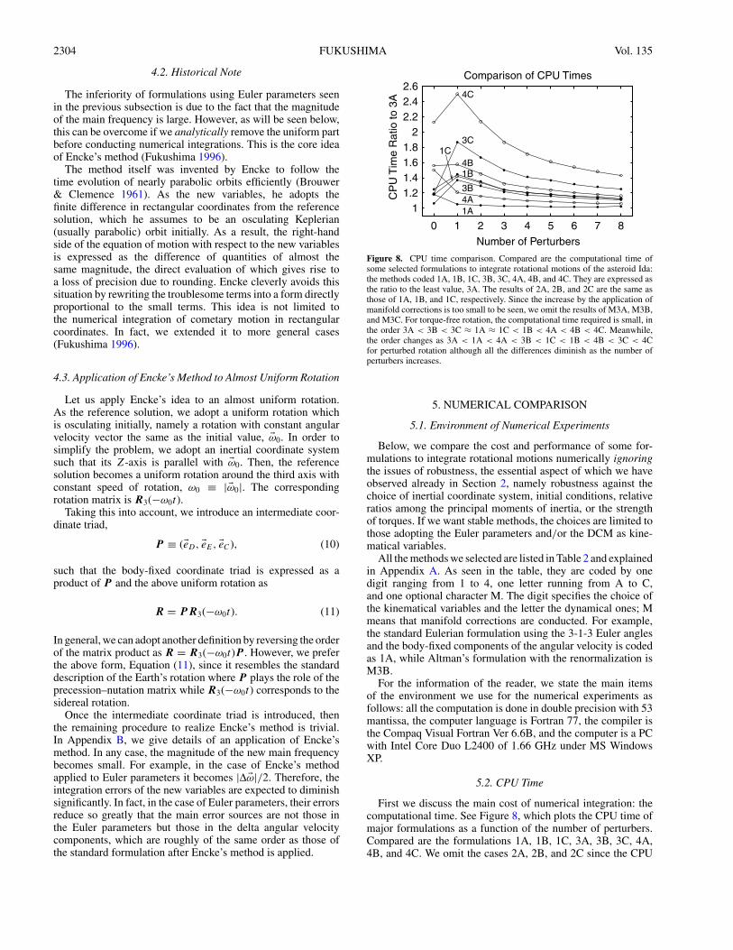
Figure 8. CPU time comparison. Compared are the computational time ofsome selected formulations to integrate rotational motions of the asteroid Ida:the methods coded 1A, 1B, 1C, 3B, 3C, 4A, 4B, and 4C. They are expressed asthe ratio to the least value, 3A. The results of 2A, 2B, and 2C are the same asthose of 1A, 1B, and 1C, respectively. Since the increase by the application ofmanifold corrections is too small to be seen, we omit the results of M3A, M3B,and M3C. For torque-free rotation, the computational time required is small, inthe order 3A < 3B < 3C ≈ 1A ≈ 1C < 1B < 4A < 4B < 4C. Meanwhile,the order changes as 3A < 1A < 4A < 3B < 1C < 1B < 4B < 3C < 4Cfor perturbed rotation although all the differences diminish as the number ofperturbers increases.
5. NUMERICAL COMPARISON
5.1. Environment of Numerical Experiments
Below, we compare the cost and performance of some for-mulations to integrate rotational motions numerically ignoringthe issues of robustness, the essential aspect of which we haveobserved already in Section 2, namely robustness against thechoice of inertial coordinate system, initial conditions, relativeratios among the principal moments of inertia, or the strengthof torques. If we want stable methods, the choices are limited tothose adopting the Euler parameters and/or the DCM as kine-matical variables.
All the methods we selected are listed in Table 2 and explainedin Appendix A. As seen in the table, they are coded by onedigit ranging from 1 to 4, one letter running from A to C,and one optional character M. The digit specifies the choice ofthe kinematical variables and the letter the dynamical ones; Mmeans that manifold corrections are conducted. For example,the standard Eulerian formulation using the 3-1-3 Euler anglesand the body-fixed components of the angular velocity is codedas 1A, while Altman’s formulation with the renormalization isM3B.
For the information of the reader, we state the main itemsof the environment we use for the numerical experiments asfollows: all the computation is done in double precision with 53mantissa, the computer language is Fortran 77, the compiler isthe Compaq Visual Fortran Ver 6.6B, and the computer is a PCwith Intel Core Duo L2400 of 1.66 GHz under MS WindowsXP.
5.2. CPU Time
First we discuss the main cost of numerical integration: thecomputational time. See Figure 8, which plots the CPU time ofmajor formulations as a function of the number of perturbers.Compared are the formulations 1A, 1B, 1C, 3A, 3B, 3C, 4A,4B, and 4C. We omit the cases 2A, 2B, and 2C since the CPU
No. 6, 2008 NUMERICAL INTEGRATION OF ROTATIONAL MOTION 2305
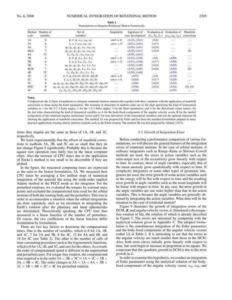
Table 2Formulations to Integrate Rotational Motion Numerically
Method Number of Set of Singularity Equations of Evaluation of Evaluation of Manifoldcode variables variables time development (eA, eB, eC ) (ωA,ωB, ωC ) corrections
1A 6 ψ, θ, φ, ωA, ωB, ωC sin θ = 0 (A12), (A41) (A5) . . . . . .
2A 6 ξ, η, ζ, ωA, ωB, ωC cos η = 0 (A21), (A41) (A17) . . . . . .
3A 7 q0, q1, q2, q3, ωA, ωB, ωC . . . (A35), (A41) (A24) . . . . . .
M3A 7 q0, q1, q2, q3, ωA, ωB, ωC . . . (A35), (A41) (A24) . . . (8)4A 12 eA, eB, eC, ωA, ωB, ωC . . . (A39), (A41) . . . . . . . . .
1B 6 ψ, θ, φ, LX,LY , LZ sin θ = 0 (A12), (A48) (A5) (A50) . . .
2B 6 ξ, η, ζ, LX, LY , LZ cos η = 0 (A21), (A48) (A17) (A50) . . .
3B 7 q0, q1, q2, q3, LX, LY , LZ . . . (A35), (A48) (A24) (A50) . . .
M3B 7 q0, q1, q2, q3, LX, LY , LZ . . . (A35), (A48) (A24) (A50) (8)4B 12 eA, eB, eC, LX, LY , LZ . . . (A39), (A48) . . . (A50) . . .
1C 6 ψ, θ, φ, dψ/dt, dθ/dt, dφ/dt sin θ = 0 (A52) (A5) (A10) . . .
2C 6 ξ, η, ζ, dξ/dt, dη/dt, dζ/dt cos η = 0 (A54) (A17) (A20) . . .
3C 8 q0, q1, q2, q3, dq0/dt, dq1/dt, dq2/dt, dq3/dt . . . (A56) (A24) (A34) . . .
M3C 8 q0, q1, q2, q3, dq0/dt, dq1/dt, dq2/dt, dq3/dt . . . (A56) (A24) (A34) (8), (9)4C 18 eA, eB, eC, deA/dt, deB/dt, deC/dt . . . (A58) . . . (A59) . . .
Notes.Compared are the 12 basic formulations to integrate rotational motions numerically together with three variations with the application of manifoldcorrections to those using the Euler parameters. The meaning of characters in method codes are (i) the digit specifying the kind of kinematicalvariables as 1 for the 3-1-3 Euler angles, 2 for the 1-2-3 Euler angles, 3 for the Euler parameters, and 4 for the directional cosine matrix; (ii)the last letter characterizing the kind of dynamical variables as A for the body-fixed components of the angular velocity vector, B for the inertialcomponents of the rotational angular momentum vector, and C for time derivatives of the kinematical variables; and (iii) the optional character Mshowing the application of manifold corrections. The method 1A was proposed by Euler and has been the standard formulation adopted in manypractical applications treating almost uniform rotations such as the Earth rotation. The method 3B was first proposed by Altman (1972).
times they require are the same as those of 1A, 1B, and 1C,respectively.
We learn experimentally that the effects of manifold correc-tions to methods 3A, 3B, and 3C are so small that they donot change Figure 8 significantly. Probably this is because thesquare root operation runs fairly fast in the latest computerchips. Also the increase of CPU times due to the applicationof Encke’s method is too small to be discernible if they areplotted.
In the figure, the measured computing times are expressedas the ratio to the fastest formulation, 3A. We measured theirCPU times by averaging a few million steps of numericalintegration of the asteroid Ida using the tenth-order implicitAdams method in the PECE mode as the integrator. For theperturbed rotations, we evaluated the torques by external masspoints and excluded the computational time used for the orbitalmotions of both the rotating body and the perturbers. This was inorder to accommodate a situation when the orbital integrationsare done separately, such as we encounter in integrating theEarth’s rotation after the planetary and lunar ephemeridesare determined. Theoretically speaking, the CPU time thusmeasured is a linear function of the number of perturbers.Of course, the two coefficients of the linear function differformulation by formulation.
There are two key factors to determine the computationaltimes. One is the number of variables, which is 6 for 1A, 1B,and 1C, 7 for 3A and 3B, 8 for 3C, 12 for 4A and 4B, and18 for 4C (see Table 2). The other is the number of calls oftime-consuming procedures such as the trigonometric functions,which is 6 for 1A, 1B, and 1C, and zero for the others. As a result,the order of computational speed is different in the unperturbedand perturbed cases. For torque-free rotation, the computationaltime required is in the order 3A < 3B < 3C ≈ 1A ≈ 1C < 1B <4A < 4B < 4C. The order changes to 3A < 1A < 4A < 3B <1C < 1B < 4B < 3C < 4C for perturbed rotation.
5.3. Growth of Integration Error
Before conducting a performance comparison of various for-mulations, we will discuss the general features of the integrationerrors of rotational motions. In the case of orbital motions, ifordinary integrators such as Runge–Kutta or Stormer–Cowellmethods are used, the errors in action variables such as thesemi-major axis or the eccentricity grow linearly with respectto time. In contrast, those of angle variables, especially that ofthe mean anomaly grow quadratically with respect to time. Ifsymplectic integrators or some other types of geometric inte-grators are used, the error growth of some action variables suchas the energy will be flat with respect to time and the resultingerror growth in angle variables such as the mean longitude willbe linear with respect to time. In any case, the error growth inthe angle variables are one order higher than that in the actionvariables. This is because the angle variables are generally ob-tained by integrating the action variables. What then will be thesituation in the case of rotational motion?
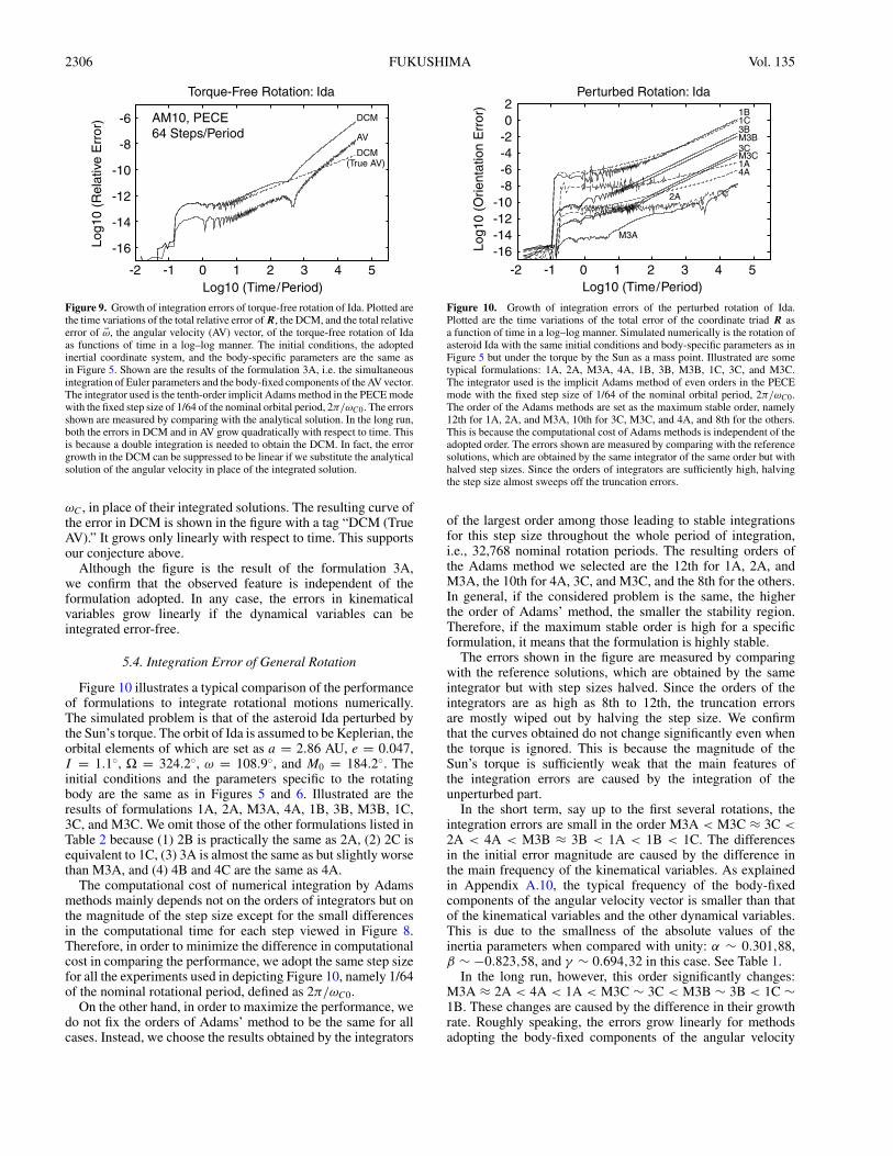
Figure 9 illustrates the growth of integration errors of theDCM, R, and angular velocity vector, ω. Simulated is the torque-free rotation of Ida, the solution of which is already describedin Figure 5. The errors are measured by comparing with theanalytical solution given in Appendix C. The adopted formu-lation is the simultaneous integration of the Euler parametersand the body-fixed components of the angular velocity vectorscoded 3A in Table 2. It is interesting to see that the errors inthe angular velocity are much smaller than those in the DCM.Also, both error curves initially grow linearly with respect totime, but soon begin to increase in proportion to its square. Weconjecture that this quadratic growth in DCM is due to the errorgrowth in ω.
In order to examine this hypothesis, we conduct an integrationof Euler parameters using the analytical solution of the body-fixed components of the angular velocity vector, ωA, ωB , and
2306 FUKUSHIMA Vol. 135
-16
-14
-12
-10
-8
-6
-2 -1 0 1 2 3 4 5
Log1
0 (R
elat
ive
Err
or)
Log10 (Time/Period)
Torque-Free Rotation: Ida
AM10, PECE64 Steps/Period
DCM
DCM(True AV)
AV
Figure 9. Growth of integration errors of torque-free rotation of Ida. Plotted arethe time variations of the total relative error of R, the DCM, and the total relativeerror of ω, the angular velocity (AV) vector, of the torque-free rotation of Idaas functions of time in a log–log manner. The initial conditions, the adoptedinertial coordinate system, and the body-specific parameters are the same asin Figure 5. Shown are the results of the formulation 3A, i.e. the simultaneousintegration of Euler parameters and the body-fixed components of the AV vector.The integrator used is the tenth-order implicit Adams method in the PECE modewith the fixed step size of 1/64 of the nominal orbital period, 2π/ωC0. The errorsshown are measured by comparing with the analytical solution. In the long run,both the errors in DCM and in AV grow quadratically with respect to time. Thisis because a double integration is needed to obtain the DCM. In fact, the errorgrowth in the DCM can be suppressed to be linear if we substitute the analyticalsolution of the angular velocity in place of the integrated solution.
ωC , in place of their integrated solutions. The resulting curve ofthe error in DCM is shown in the figure with a tag “DCM (TrueAV).” It grows only linearly with respect to time. This supportsour conjecture above.
Although the figure is the result of the formulation 3A,we confirm that the observed feature is independent of theformulation adopted. In any case, the errors in kinematicalvariables grow linearly if the dynamical variables can beintegrated error-free.
5.4. Integration Error of General Rotation
Figure 10 illustrates a typical comparison of the performanceof formulations to integrate rotational motions numerically.The simulated problem is that of the asteroid Ida perturbed bythe Sun’s torque. The orbit of Ida is assumed to be Keplerian, theorbital elements of which are set as a = 2.86 AU, e = 0.047,I = 1.1, Ω = 324.2, ω = 108.9, and M0 = 184.2. Theinitial conditions and the parameters specific to the rotatingbody are the same as in Figures 5 and 6. Illustrated are theresults of formulations 1A, 2A, M3A, 4A, 1B, 3B, M3B, 1C,3C, and M3C. We omit those of the other formulations listed inTable 2 because (1) 2B is practically the same as 2A, (2) 2C isequivalent to 1C, (3) 3A is almost the same as but slightly worsethan M3A, and (4) 4B and 4C are the same as 4A.
The computational cost of numerical integration by Adamsmethods mainly depends not on the orders of integrators but onthe magnitude of the step size except for the small differencesin the computational time for each step viewed in Figure 8.Therefore, in order to minimize the difference in computationalcost in comparing the performance, we adopt the same step sizefor all the experiments used in depicting Figure 10, namely 1/64of the nominal rotational period, defined as 2π/ωC0.
On the other hand, in order to maximize the performance, wedo not fix the orders of Adams’ method to be the same for allcases. Instead, we choose the results obtained by the integrators
-16-14-12-10
-8-6-4-202
-2 -1 0 1 2 3 4 5
Log1
0 (O
rient
atio
n E
rror
)
Log10 (Time/Period)
Perturbed Rotation: Ida
1B1C3BM3B3CM3C1A4A
2A
M3A
Figure 10. Growth of integration errors of the perturbed rotation of Ida.Plotted are the time variations of the total error of the coordinate triad R asa function of time in a log–log manner. Simulated numerically is the rotation ofasteroid Ida with the same initial conditions and body-specific parameters as inFigure 5 but under the torque by the Sun as a mass point. Illustrated are sometypical formulations: 1A, 2A, M3A, 4A, 1B, 3B, M3B, 1C, 3C, and M3C.The integrator used is the implicit Adams method of even orders in the PECEmode with the fixed step size of 1/64 of the nominal orbital period, 2π/ωC0.The order of the Adams methods are set as the maximum stable order, namely12th for 1A, 2A, and M3A, 10th for 3C, M3C, and 4A, and 8th for the others.This is because the computational cost of Adams methods is independent of theadopted order. The errors shown are measured by comparing with the referencesolutions, which are obtained by the same integrator of the same order but withhalved step sizes. Since the orders of integrators are sufficiently high, halvingthe step size almost sweeps off the truncation errors.
of the largest order among those leading to stable integrationsfor this step size throughout the whole period of integration,i.e., 32,768 nominal rotation periods. The resulting orders ofthe Adams method we selected are the 12th for 1A, 2A, andM3A, the 10th for 4A, 3C, and M3C, and the 8th for the others.In general, if the considered problem is the same, the higherthe order of Adams’ method, the smaller the stability region.Therefore, if the maximum stable order is high for a specificformulation, it means that the formulation is highly stable.
The errors shown in the figure are measured by comparingwith the reference solutions, which are obtained by the sameintegrator but with step sizes halved. Since the orders of theintegrators are as high as 8th to 12th, the truncation errorsare mostly wiped out by halving the step size. We confirmthat the curves obtained do not change significantly even whenthe torque is ignored. This is because the magnitude of theSun’s torque is sufficiently weak that the main features ofthe integration errors are caused by the integration of theunperturbed part.
In the short term, say up to the first several rotations, theintegration errors are small in the order M3A < M3C ≈ 3C <2A < 4A < M3B ≈ 3B < 1A < 1B < 1C. The differencesin the initial error magnitude are caused by the difference inthe main frequency of the kinematical variables. As explainedin Appendix A.10, the typical frequency of the body-fixedcomponents of the angular velocity vector is smaller than thatof the kinematical variables and the other dynamical variables.This is due to the smallness of the absolute values of theinertia parameters when compared with unity: α ∼ 0.301,88,β ∼ −0.823,58, and γ ∼ 0.694,32 in this case. See Table 1.
In the long run, however, this order significantly changes:M3A ≈ 2A < 4A < 1A < M3C ∼ 3C < M3B ∼ 3B < 1C ∼1B. These changes are caused by the difference in their growthrate. Roughly speaking, the errors grow linearly for methodsadopting the body-fixed components of the angular velocity
No. 6, 2008 NUMERICAL INTEGRATION OF ROTATIONAL MOTION 2307
-16-14-12-10-8-6-4-202
-2 -1 0 1 2 3 4 5
Log1
0 (O
rient
atio
n E
rror
)
Log10 (Time/Period)
Perturbed Rotation: Triaxial Earth
4A
3B
M3C
3A M3A
1B 1A
ME3A
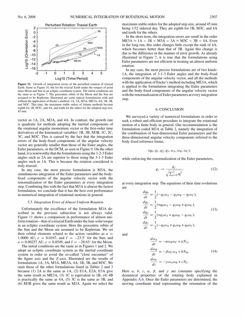
Figure 11. Growth of integration errors of the perturbed rotation of triaxialEarth. Same as Figure 10, but for the triaxial Earth under the torques of pointmass Moon and Sun in an ecliptic coordinate system. The initial conditions arethe same as in Figure 7. The geocentric orbits of the Moon and the Sun areassumed to be Keplerian. Illustrated are some typical formulations with andwithout the application of Encke’s method; 1A, 3A, M3A, ME3A, 4A, 1B, 3B,and M3C. This time, the maximum stable orders of Adams methods becomeeighth for 1B, M3C, and 4A, and tenth for the others for the adopted step size,45 min.
vector as 1A, 2A, M3A, and 4A. In contrast, the growth rateis quadratic for methods adopting the inertial components ofthe rotational angular momentum vector or the first-order timederivatives of the kinematical variables: 1B, 3B, M3B, 1C, 2C,3C, and M3C. This is caused by the fact that the integrationerrors of the body-fixed components of the angular velocityvector are generally smaller than those of the Euler angles, theEuler parameters, or the DCM, as seen in Figure 9. On the otherhand, it is noteworthy that the formulations using the 1-2-3 Eulerangles such as 2A are superior to those using the 3-1-3 Eulerangles such as 1A. This is because the rotation considered istruly triaxial.
In any case, the most precise formulation is M3A, thesimultaneous integration of the Euler parameters and the body-fixed components of the angular velocity vector with therenormalization of the Euler parameters at every integrationstep. Combining this with the fact that M3A is almost the fastestformulation, we conclude that it has the best cost performancein numerical integration of rotational motions in general.
5.5. Integration Error of Almost Uniform Rotation
Unfortunately the excellence of the formulation M3A de-scribed in the previous subsection is not always valid.Figure 11 shows a comparison in performance of almost uni-form rotation—that of a triaxial Earth under the luni-solar torquein an ecliptic coordinate system. Here the geocentric orbits ofthe Sun and the Moon are assumed to be Keplerian. We settheir orbital elements related to the action variables as a =1.0000 AU, e = 0.0167, and I = −23.5 for the Sun, anda = 0.00257 AU, e = 0.0549, and I = −28.63 for the Moon.
The initial conditions are the same as in Figures 1 and 2. Weadopt an ecliptic coordinate system as the inertial coordinatesystem in order to avoid the so-called “close encounter” ofthe figure axis and the Z-axis. Illustrated are the results offormulations 1A, 3A, M3A, ME3A, 4A, 1B, 3B, and M3C. Weomit those of the other formulations listed in Tables 2 and 3because (1) 2A is the same as 1A, (2) E1A, E2A, E3A givethe same result as ME3A, (3) 1C is equivalent to 1B, (4) 4Bis practically the same as 4A, (5) 3C is the same as 3B, and(6) M3B gives the same result as M3A. Again we select the
maximum stable orders for the adopted step size, around 45 minbeing 1/32 sidereal day. They are eighth for 1B, M3C, and 4Aand tenth for the others.
In the short term, the integration errors are small in the orderME3A ≈ 1A < 1B < M3A < 3A ≈ M3C < 3B < 4A. Evenin the long run, this order changes little except the rank of 4A,which becomes better than that of 3B. Again this change isdue to the difference in the manner of error growth. As alreadyillustrated in Figure 7, it is true that the formulations usingEuler parameters are not efficient in treating an almost uniformrotation.
In any case, the most precise formulations are of two kinds:1A, the integration of 3-1-3 Euler angles and the body-fixedcomponents of the angular velocity vector, and all the methodswith the application of Encke’s method including ME3A, whichis applied to the formulation integrating the Euler parametersand the body-fixed components of the angular velocity vectorwith the renormalization of Euler parameters at every integrationstep.
6. CONCLUSION
We surveyed a variety of numerical formulations in order toseek a robust and efficient procedure to integrate the rotationalmotion of a finite body in general. Our recommendation is theformulation coded M3A in Table 2, namely the integration ofthe combination of four-dimensional Euler parameters and thethree-dimensional angular velocity components referred to thebody-fixed reference frame,
(q0, q1, q2, q3, ωA, ωB, ωC),
while enforcing the renormalization of the Euler parameters,
qj → qj√∑3i=0 q2
i
, (12)
at every integration step. The equations of their time evolutionsare
dq0
dt= 1
2(−q1ωA − q2ωB − q3ωC),
dq1
dt= 1
2(+q0ωA − q3ωB + q2ωC),
dq2
dt= 1
2(+q3ωA + q0ωB − q1ωC),
dq3
dt= 1
2(−q2ωA + q1ωB + q0ωC),
(13)
anddωA
dt= −αωBωC + aNA,
dωB
dt= −βωCωA + bNB,
dωC
dt= −γωAωB + cNC.
(14)
Here a, b, c, α, β, and γ are constants specifying thedynamical properties of the rotating body explained inAppendix A.6. Once the Euler parameters are determined, themoving coordinate triad representing the orientation of the
2308 FUKUSHIMA Vol. 135
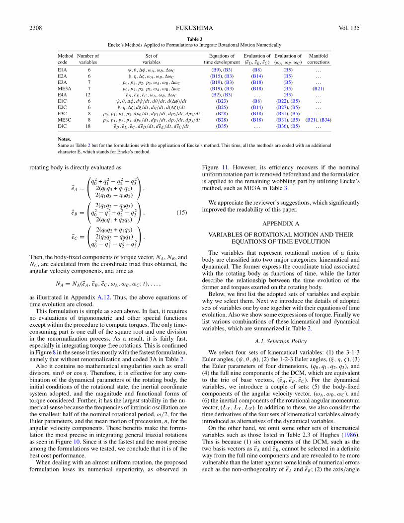
Table 3Encke’s Methods Applied to Formulations to Integrate Rotational Motion Numerically
Method Number of Set of Equations of Evaluation of Evaluation of Manifoldcode variables variables time development (eD, eE, eC ) (ωA, ωB, ωC ) corrections
E1A 6 ψ, θ, ∆φ, ωA, ωB, ∆ωC (B9), (B3) (B8) (B5) . . .
E2A 6 ξ, η, ∆ζ, ωA, ωB, ∆ωC (B15), (B3) (B14) (B5) . . .
E3A 7 p0, p1, p2, p3, ωA, ωB, ∆ωC (B19), (B3) (B18) (B5) . . .
ME3A 7 p0, p1, p2, p3, ωA, ωB, ∆ωC (B19), (B3) (B18) (B5) (B21)E4A 12 eD, eE, eC, ωA, ωB, ∆ωC (B2), (B3) . . . (B5) . . .
E1C 6 ψ, θ, ∆φ, dψ/dt, dθ/dt, d(∆φ)/dt (B23) (B8) (B22), (B5) . . .
E2C 6 ξ, η, ∆ζ, dξ/dt, dη/dt, d(∆ζ )/dt (B25) (B14) (B27), (B5) . . .
E3C 8 p0, p1, p2, p3, dp0/dt, dp1/dt, dp2/dt, dp3/dt (B28) (B18) (B31), (B5) . . .
ME3C 8 p0, p1, p2, p3, dp0/dt, dp1/dt, dp2/dt, dp3/dt (B28) (B18) (B31), (B5) (B21), (B34)E4C 18 eD, eE, eC, deD/dt, deE/dt, deC/dt (B35) . . . (B36), (B5) . . .
Notes.Same as Table 2 but for the formulations with the application of Encke’s method. This time, all the methods are coded with an additionalcharacter E, which stands for Encke’s method.
rotating body is directly evaluated as
eA =⎛⎝q2
0 + q21 − q2
2 − q23
2(q0q3 + q1q2)2(q1q3 − q0q2)
⎞⎠ ,
eB =⎛⎝ 2(q1q2 − q0q3)
q20 − q2
1 + q22 − q2
32(q0q1 + q2q3)
⎞⎠ ,
eC =⎛⎝ 2(q0q2 + q1q3)
2(q2q3 − q0q1)q2
0 − q21 − q2
2 + q23
⎞⎠ .
(15)
Then, the body-fixed components of torque vector, NA, NB , andNC , are calculated from the coordinate triad thus obtained, theangular velocity components, and time as
NA = NA(eA, eB, eC, ωA, ωB, ωC; t), . . . ,
as illustrated in Appendix A.12. Thus, the above equations oftime evolution are closed.
This formulation is simple as seen above. In fact, it requiresno evaluations of trigonometric and other special functionsexcept within the procedure to compute torques. The only time-consuming part is one call of the square root and one divisionin the renormalization process. As a result, it is fairly fast,especially in integrating torque-free rotations. This is confirmedin Figure 8 in the sense it ties mostly with the fastest formulation,namely that without renormalization and coded 3A in Table 2.
Also it contains no mathematical singularities such as smalldivisors, sin θ or cos η. Therefore, it is effective for any com-bination of the dynamical parameters of the rotating body, theinitial conditions of the rotational state, the inertial coordinatesystem adopted, and the magnitude and functional forms oftorque considered. Further, it has the largest stability in the nu-merical sense because the frequencies of intrinsic oscillation arethe smallest: half of the nominal rotational period, ω/2, for theEuler parameters, and the mean motion of precession, n, for theangular velocity components. These benefits make the formu-lation the most precise in integrating general triaxial rotationsas seen in Figure 10. Since it is the fastest and the most preciseamong the formulations we tested, we conclude that it is of thebest cost performance.
When dealing with an almost uniform rotation, the proposedformulation loses its numerical superiority, as observed in
Figure 11. However, its efficiency recovers if the nominaluniform rotation part is removed beforehand and the formulationis applied to the remaining wobbling part by utilizing Encke’smethod, such as ME3A in Table 3.
We appreciate the reviewer’s suggestions, which significantlyimproved the readability of this paper.
APPENDIX A
VARIABLES OF ROTATIONAL MOTION AND THEIREQUATIONS OF TIME EVOLUTION
The variables that represent rotational motion of a finitebody are classified into two major categories: kinematical anddynamical. The former express the coordinate triad associatedwith the rotating body as functions of time, while the latterdescribe the relationship between the time evolution of theformer and torques exerted on the rotating body.
Below, we first list the adopted sets of variables and explainwhy we select them. Next we introduce the details of adoptedsets of variables one by one together with their equations of timeevolution. Also we show some expressions of torque. Finally welist various combinations of these kinematical and dynamicalvariables, which are summarized in Table 2.
A.1. Selection Policy
We select four sets of kinematical variables: (1) the 3-1-3Euler angles, (ψ, θ, φ), (2) the 1-2-3 Euler angles, (ξ, η, ζ ), (3)the Euler parameters of four dimensions, (q0, q1, q2, q3), and(4) the full nine components of the DCM, which are equivalentto the trio of base vectors, (eA, eB, eC). For the dynamicalvariables, we introduce a couple of sets: (5) the body-fixedcomponents of the angular velocity vector, (ωA,ωB, ωC), and(6) the inertial components of the rotational angular momentumvector, (LX,LY , LZ). In addition to these, we also consider thetime derivatives of the four sets of kinematical variables alreadyintroduced as alternatives of the dynamical variables.
On the other hand, we omit some other sets of kinematicalvariables such as those listed in Table 2.3 of Hughes (1986).This is because (1) six components of the DCM, such as thetwo basis vectors as eA and eB , cannot be selected in a definiteway from the full nine components and are revealed to be morevulnerable than the latter against some kinds of numerical errorssuch as the non-orthogonality of eA and eB ; (2) the axis/angle

No. 6, 2008 NUMERICAL INTEGRATION OF ROTATIONAL MOTION 2309
variables of four dimensions or the Euler axis and angle, (ϕ, n),with a constraint |n| = 1 contain a singularity of the anglevariable, ϕ = mπ , where m is an arbitrary integer; (3) the axis/angle variables of three dimensions or the so-called rotationvector, ϕ ≡ ϕn, with the same constraint |n| = 1 have thesame singularity, | ϕ| = mπ ; (4) the three-dimensional Euler–Rodriguez parameters or the Gibbs vector, p ≡ [tan(ϕ/2)]n,with the same constraint |n| = 1 have a singularity, | p| = ∞,which is nothing but the same condition ϕ = mπ ; (5) the Eulerparameters of three dimensions, ε ≡ [sin(ϕ/2)]n, with the sameconstraint |n| = 1 have a singularity, |ε| = 1, which againmeans the same condition, ϕ = mπ .
Also we do not discuss a couple of sets of dynamicalvariables because (6) the body-fixed components of the angularmomentum, (LA,LB,LC), are mathematically equivalent tothose of the angular velocity vector for a rigid body sincecomponent-dependent proportional relations hold as LA =AωA, LB = BωB , and LC = CωC , and (7) the inertialcomponents of the angular velocity vector, (ωX,ωY , ωZ), aremore difficult to treat than those of the angular momentumvector despite the performance being almost the same.
A.2. 3-1-3 Euler Angles
We describe the kinematical variables as a set of variables toexpress the inertial components of a moving coordinate triad,namely three orthonormal vectors attached to the rotating body,eA, eB , and eC . Sometimes they are collectively called the DCM,which is expressed as
R ≡ (eA, eB, eC). (A1)
The Euler angles are three angles used to express the DCM inthe form of a triple product of the fundamental rotation matricesas
R = Ri(−x)Rj (−y)Rk(−z). (A2)
Here the indices i, j , and k run from 1 to 3 while satisfyingthe nondegenerate conditions, i = j and j = k. Also R(w)denotes the fundamental rotation matrix around the th axis bythe angle w. Namely,
R1(x) ≡(
1 0 00 cos x sin x0 −sin x cos x
),
R2(y) ≡(
cos y 0 −sin y0 1 0
sin y 0 cos y
),
R3(z) ≡(
cos z sin z 0−sin z cos z 0
0 0 1
).
(A3)
There are 12 combinations of indices (i,j,k). See Table 2.2of Hughes (1986). They are categorized into two groups: (1)six combinations with the condition i = k, namely (1, 2,1), (1, 3, 1), (2, 1, 2), (2, 3, 2), (3, 1, 3), and (3, 2, 3),and (2) another six where i = k, namely (1, 2, 3),(1, 3, 2), (2, 1, 3), (2, 3, 1), (3, 1, 2), and (3, 2, 1).
The most popular trio of the indices belongs to the first group:the 3-1-3 convention where i = k = 3 and j = 1. To describethe angles, we adopt the continental notations, x = ψ , y = θ ,and z = φ:
R = R3(−ψ)R1(−θ )R3(−φ). (A4)
X
Y
A
N
H
θ(π / 2)−ξ
η ζ−φ
ψ
φ
Prime Meridian
Reference Plane
Body Equator
·
·
··
·
Figure 12. Geometrical relation between the 3-1-3 and 1-2-3 Euler angles.Schematically shown are the arcs and angles defining the 3-1-3 Euler anglesand the 1-2-3 Euler angles for the same rotation operation. They are depictedhere on a part of the unit spherical surface. Points X, Y , and A represent thedirections of the X-, Y -, and A-axes of coordinate triads, respectively. Point N
is the node, namely one of two intersections of the body equator, i.e. the planecontaining the A- and B-axes, and the reference plane, i.e. the X–Y plane. AlsoPoint H is the foot of X on the body equator. Then the 3-1-3 Euler angles aregeometrically defined such that (1) ψ is the length of arc XN, (2) θ is the angleYNA, and (3) φ is the length of arc NA. On the other hand, the 1-2-3 Euler anglesare geometrically defined such that (1) ξ is 90minus the angle HXN, (2) η isthe length of arc XH, and (3) ζ is the length of arc HA.
Their geometrical definitions are illustrated in Figure 12, whichshows a maginified view of a part of the celestial sphere. The 3-1-3 Euler angles are geometrically defined such that (1) ψ is thelength of arc XN, (2) θ is the angle YNA, and (3) φ is the lengthof arc NA, where X, Y , and A represent the directions of the X-,Y -, and A-axes of coordinate triads, respectively, and the nodalpoint N is one of two intersections of the body equator andthe reference plane. Note that Goldstein et al. (2002) choosethe British notation where the role of φ and ψ are reversed.The coordinate triad of the 3-1-3 Euler angles based on thecontinental notations is explicitly expressed as
eA =(
cos φ cos ψ − sin φ cos θ sin ψcos φ sin ψ + sin φ cos θ cos ψ
sin φ sin θ
),
eB =(−sin φ cos ψ − cos φ cos θ sin ψ
−sin φ sin ψ + cos φ cos θ cos ψcos φ sin θ
),
eC =(
sin θ sin ψ−sin θ cos ψ
cos θ
).
(A5)
On the other hand, a reverse transformation providing the threeEuler angles from the nine components of the DCM, which isnot unique, is given as
ψ = atan2[(eC)X, − (eC)Y ],θ = cos−1[(eC)Z],
φ = atan2[(eA)Z, (eB)Z],(A6)
where we assume that θ is in the range 0 θ < π . Alsoatan2(y, x) is the two-argument arctangent function realized insome computer languages such as C or Fortran, which computestan−1(y/x) while taking the signs of x and y into account.
By differentiating the expression of the DCM, Equation (A4),we evaluate the vector expression of the angular velocity vector
2310 FUKUSHIMA Vol. 135
as
ω ≡ (ωX,ωY , ωZ)T =(
dψ
dt
)eZ +
(dθ
dt
)eN +
(dφ
dt
)eC,
(A7)where eZ is the third axis base vector of the inertial coordinatesystem and
eN ≡(
cos ψsin ψ
0
)(A8)
is the first axis base vector of the first intermediary DCM,R3(−ψ). The above vectorial expression is rewritten in inertialcomponents as
ωX =(
dθ
dt
)cos ψ +
(dφ
dt
)sin θ sin ψ,
ωY =(
dθ
dt
)sin ψ −
(dφ
dt
)sin θ cos ψ,
ωZ =(
dψ
dt
)+
(dφ
dt
)cos θ,
(A9)
which is translated into body-fixed components as
ωA =(
dψ
dt
)sin θ sin φ +
(dθ
dt
)cos φ,
ωB =(
dψ
dt
)sin θ cos φ −
(dθ
dt
)sin φ,
ωC =(
dψ
dt
)cos θ +
(dφ
dt
),
(A10)
where
ωA ≡ ω · eA, ωB ≡ ω · eB, ωC ≡ ω · eC (A11)
are the body-fixed components of the angular velocity vector,ω.
Solving the last expressions with respect to the time deriva-tives of the Euler angles, we obtain the time evolution equationsof these Euler angles as
dψ
dt= ωF
sin θ,
dθ
dt= ωA cos φ − ωB sin φ,
dφ
dt= ωC −
( ωF
tan θ
),
(A12)
whereωF ≡ ωA sin φ + ωB cos φ. (A13)
In these time evolution equations, there exists a singularity,θ = mπ , where m is an arbitrary integer. This fact, namely thatthe second Euler angle has a singularity of mπ , is a commonfeature to all other five combinations of the group where i = k.See Table 2.2 of Hughes (1986).
A.3. 1-2-3 Euler Angles
We select the 1-2-3 convention as a typical example of thesecond group of Euler angles where the first and the third indicesare different from each other. In this case, we use the notationsx = ξ , y = η, and z = ζ , while i = 1, j = 2, and k = 3:
R = R1(−ξ )R2(−η)R3(−ζ ). (A14)
See Figure 12 for the geometrical relation between the 1-2-3Euler angles and the 3-1-3 Euler angles. Mathematically, theyare related to each other as
ξ = tan−1(cos ψ tan θ ),
η = sin−1(sin ψ sin θ ),
ζ = φ + tan−1(tan ψ cos θ ),
(A15)
and
ψ = tan−1(sin ξ tan η),
θ = cos−1(cos ξ cos η),
φ = ζ − tan−1(cot ξ sin η).
(A16)
The expressions of the coordinate triad in terms of the 1-2-3Euler angles are
eA =(
cos ζ cos ηsin ζ cos ξ + cos ζ sin η sin ξsin ζ sin ξ − cos ζ sin η cos ξ
),
eB =( −sin ζ cos η
cos ζ cos ξ − sin ζ sin η sin ξcos ζ sin ξ + sin ζ sin η cos ξ
),
eC =(
sin η−cos η sin ξcos η cos ξ
).
(A17)
A reverse transformation, which again is not unique, is obtainedas
ξ = atan2[−(eC)Y ,(eC)Z],
η = sin−1[(eC)X],
ζ = atan2[−(eB)X,(eA)X],
(A18)
where we assume that η is in the range |η| π/2. As in the caseof the 3-1-3 Euler angles, we evaluate the inertial componentsof the angular velocity vector in terms of the 1-2-3 Euler anglesas (
ωX
ωY
ωZ
)=
(dξ
dt
) (100
)+
(dη
dt
) (0
cos ξsin ξ
)
+
(dζ
dt
) (sin η
−cos η sin ξcos η cos ξ
), (A19)
which leads to the body-fixed component expressions
ωA =(
dξ
dt
)cos η cos ζ +
(dη
dt
)sin ζ,
ωB = −(
dξ
dt
)cos η sin ζ +
(dη
dt
)cos ζ,
ωC =(
dξ
dt
)sin η +
(dζ
dt
).
(A20)
The resulting time evolution equations of the 1-2-3 Euler anglesbecome somewhat different from those of the 3-1-3 Euler angles:
dξ
dt= ωG
cos η,
dη
dt= ωA sin ζ + ωB cos ζ,
dζ
dt= ωC − ωG tan η,
(A21)
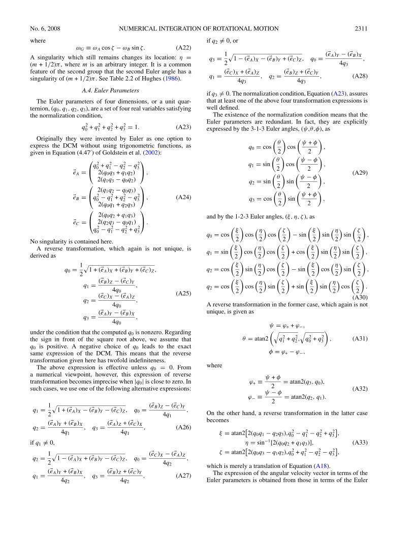
No. 6, 2008 NUMERICAL INTEGRATION OF ROTATIONAL MOTION 2311
whereωG ≡ ωA cos ζ − ωB sin ζ. (A22)
A singularity which still remains changes its location: η =(m + 1/2)π , where m is an arbitrary integer. It is a commonfeature of the second group that the second Euler angle has asingularity of (m + 1/2)π . See Table 2.2 of Hughes (1986).
A.4. Euler Parameters
The Euler parameters of four dimensions, or a unit quar-ternion, (q0, q1, q2, q3), are a set of four real variables satisfyingthe normalization condition,
q20 + q2
1 + q22 + q2
3 = 1. (A23)
Originally they were invented by Euler as one option toexpress the DCM without using trigonometric functions, asgiven in Equation (4.47′) of Goldstein et al. (2002):
eA =⎛⎝q2
0 + q21 − q2
2 − q23
2(q0q3 + q1q2)2(q1q3 − q0q2)
⎞⎠ ,
eB =⎛⎝ 2(q1q2 − q0q3)
q20 − q2
1 + q22 − q2
32(q0q1 + q2q3)
⎞⎠ ,
eC =⎛⎝ 2(q0q2 + q1q3)
2(q2q3 − q0q1)q2
0 − q21 − q2
2 + q23
⎞⎠ .
(A24)
No singularity is contained here.A reverse transformation, which again is not unique, is
derived as
q0 = 1
2
√1 + (eA)X + (eB)Y + (eC)Z,
q1 = (eB)Z − (eC)Y4q0
,
q2 = (eC)X − (eA)Z4q0
,
q3 = (eA)Y − (eB)X4q0
,
(A25)
under the condition that the computed q0 is nonzero. Regardingthe sign in front of the square root above, we assume thatq0 is positive. A negative choice of q0 leads to the exactsame expression of the DCM. This means that the reversetransformation given here has twofold indefiniteness.
The above expression is effective unless q0 = 0. Froma numerical viewpoint, however, this expression of reversetransformation becomes imprecise when |q0| is close to zero. Insuch cases, we use one of the following alternative expressions:
q1 = 1
2
√1 + (eA)X − (eB)Y − (eC)Z, q0 = (eB)Z − (eC)Y
4q1,
q2 = (eA)Y + (eB)X4q1
, q3 = (eA)Z + (eC)X4q1
, (A26)
if q1 = 0,
q2 = 1
2
√1 − (eA)X + (eB)Y − (eC)Z, q0 = (eC)X − (eA)Z
4q2,
q1 = (eA)Y + (eB)X4q2
, q3 = (eB)Z + (eC)Y4q2
, (A27)
if q2 = 0, or
q3 = 1
2
√1 − (eA)X − (eB)Y + (eC)Z, q0 = (eA)Y − (eB)X
4q3,
q1 = (eC)X + (eA)Z4q3
, q2 = (eB)Z + (eC)Y4q3
, (A28)
if q3 = 0. The normalization condition, Equation (A23), assuresthat at least one of the above four transformation expressions iswell defined.
The existence of the normalization condition means that theEuler parameters are redundant. In fact, they are explicitlyexpressed by the 3-1-3 Euler angles, (ψ,θ,φ), as
q0 = cos
(θ
2
)cos
(ψ + φ
2
),
q1 = sin
(θ
2
)cos
(ψ − φ
2
),
q2 = sin
(θ
2
)sin
(ψ − φ
2
),
q3 = cos
(θ
2
)sin
(ψ + φ
2
),
(A29)
and by the 1-2-3 Euler angles, (ξ, η, ζ ), as
q0 = cos
(ξ
2
)cos
(η
2
)cos
(ζ
2
)− sin
(ξ
2
)sin
(η
2
)sin
(ζ
2
),
q1 = sin
(ξ
2
)cos
(η
2
)cos
(ζ
2
)+ cos
(ξ
2
)sin
(η
2
)sin
(ζ
2
),
q2 = cos
(ξ
2
)sin
(η
2
)cos
(ζ
2
)− sin
(ξ
2
)cos
(η
2
)sin
(ζ
2
),
q2 = cos
(ξ
2
)cos
(η
2
)sin
(ζ
2
)+ sin
(ξ
2
)sin
(η
2
)cos
(ζ
2
).
(A30)A reverse transformation in the former case, which again is notunique, is given as
ψ = ϕ+ + ϕ−,
θ = atan2
(√q2
1 + q22 ,
√q2
0 + q23
),
φ = ϕ+ − ϕ−,
(A31)
where
ϕ+ ≡ ψ + φ
2= atan2(q3, q0),
ϕ− ≡ ψ − φ
2= atan2(q2, q1).
(A32)
On the other hand, a reverse transformation in the latter casebecomes
ξ = atan2[2(q0q1 − q2q3),q2
0 − q21 − q2
2 + q23
],
η = sin−1[2(q0q2 + q1q3)],
ζ = atan2[2(q0q3 − q1q2),q2
0 + q21 − q2
2 − q23
],
(A33)
which is merely a translation of Equation (A18).The expression of the angular velocity vector in terms of the
Euler parameters is obtained from those in terms of the Euler
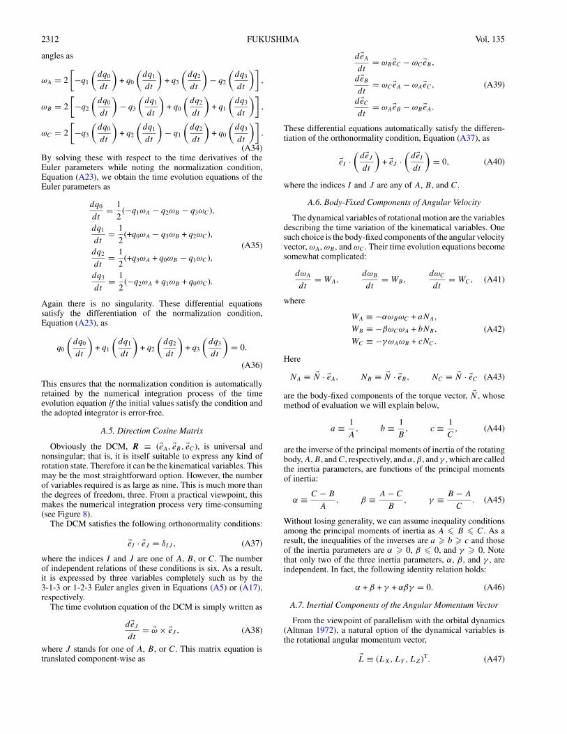
2312 FUKUSHIMA Vol. 135
angles as
ωA = 2
[−q1
(dq0
dt
)+ q0
(dq1
dt
)+ q3
(dq2
dt
)− q2
(dq3
dt
)],
ωB = 2
[−q2
(dq0
dt
)− q3
(dq1
dt
)+ q0
(dq2
dt
)+ q1
(dq3
dt
)],
ωC = 2
[−q3
(dq0
dt
)+ q2
(dq1
dt
)− q1
(dq2
dt
)+ q0
(dq3
dt
)].
(A34)By solving these with respect to the time derivatives of theEuler parameters while noting the normalization condition,Equation (A23), we obtain the time evolution equations of theEuler parameters as
dq0
dt= 1
2(−q1ωA − q2ωB − q3ωC),
dq1
dt= 1
2(+q0ωA − q3ωB + q2ωC),
dq2
dt= 1
2(+q3ωA + q0ωB − q1ωC),
dq3
dt= 1
2(−q2ωA + q1ωB + q0ωC).
(A35)
Again there is no singularity. These differential equationssatisfy the differentiation of the normalization condition,Equation (A23), as
q0
(dq0
dt
)+ q1
(dq1
dt
)+ q2
(dq2
dt
)+ q3
(dq3
dt
)= 0.
(A36)
This ensures that the normalization condition is automaticallyretained by the numerical integration process of the timeevolution equation if the initial values satisfy the condition andthe adopted integrator is error-free.
A.5. Direction Cosine Matrix
Obviously the DCM, R ≡ (eA, eB, eC), is universal andnonsingular; that is, it is itself suitable to express any kind ofrotation state. Therefore it can be the kinematical variables. Thismay be the most straightforward option. However, the numberof variables required is as large as nine. This is much more thanthe degrees of freedom, three. From a practical viewpoint, thismakes the numerical integration process very time-consuming(see Figure 8).
The DCM satisfies the following orthonormality conditions:
eI · eJ = δIJ , (A37)
where the indices I and J are one of A, B, or C. The numberof independent relations of these conditions is six. As a result,it is expressed by three variables completely such as by the3-1-3 or 1-2-3 Euler angles given in Equations (A5) or (A17),respectively.
The time evolution equation of the DCM is simply written as
deJ
dt= ω × eJ , (A38)
where J stands for one of A, B, or C. This matrix equation istranslated component-wise as
deA
dt= ωB eC − ωC eB,
deB
dt= ωC eA − ωAeC, (A39)
deC
dt= ωAeB − ωB eA.
These differential equations automatically satisfy the differen-tiation of the orthonormality condition, Equation (A37), as
eI ·(
deJ
dt
)+ eJ ·
(deI
dt
)= 0, (A40)
where the indices I and J are any of A, B, and C.
A.6. Body-Fixed Components of Angular Velocity
The dynamical variables of rotational motion are the variablesdescribing the time variation of the kinematical variables. Onesuch choice is the body-fixed components of the angular velocityvector, ωA, ωB , and ωC . Their time evolution equations becomesomewhat complicated:
dωA
dt= WA,
dωB
dt= WB,
dωC
dt= WC, (A41)
where
WA ≡ −αωBωC + aNA,
WB ≡ −βωCωA + bNB,
WC ≡ −γωAωB + cNC.
(A42)
Here
NA ≡ N · eA, NB ≡ N · eB, NC ≡ N · eC (A43)
are the body-fixed components of the torque vector, N , whosemethod of evaluation we will explain below,
a ≡ 1
A, b ≡ 1
B, c ≡ 1
C, (A44)
are the inverse of the principal moments of inertia of the rotatingbody, A, B, and C, respectively, and α, β, and γ , which are calledthe inertia parameters, are functions of the principal momentsof inertia:
α ≡ C − B
A, β ≡ A − C
B, γ ≡ B − A
C. (A45)
Without losing generality, we can assume inequality conditionsamong the principal moments of inertia as A B C. As aresult, the inequalities of the inverses are a b c and thoseof the inertia parameters are α 0, β 0, and γ 0. Notethat only two of the three inertia parameters, α, β, and γ , areindependent. In fact, the following identity relation holds:
α + β + γ + αβγ = 0. (A46)
A.7. Inertial Components of the Angular Momentum Vector
From the viewpoint of parallelism with the orbital dynamics(Altman 1972), a natural option of the dynamical variables isthe rotational angular momentum vector,
L ≡ (LX,LY , LZ)T. (A47)
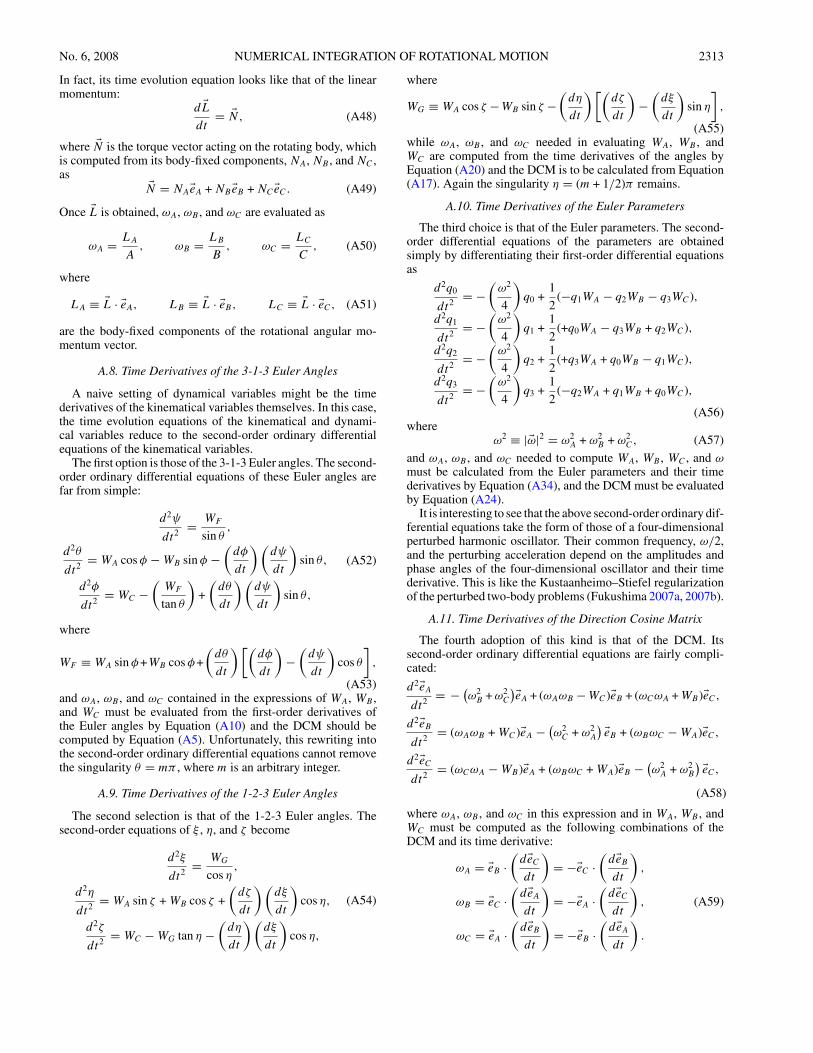
No. 6, 2008 NUMERICAL INTEGRATION OF ROTATIONAL MOTION 2313
In fact, its time evolution equation looks like that of the linearmomentum:
d Ldt
= N, (A48)
where N is the torque vector acting on the rotating body, whichis computed from its body-fixed components, NA, NB , and NC ,as
N = NAeA + NB eB + NC eC. (A49)
Once L is obtained, ωA, ωB , and ωC are evaluated as
ωA = LA
A, ωB = LB
B, ωC = LC
C, (A50)
where
LA ≡ L · eA, LB ≡ L · eB, LC ≡ L · eC, (A51)
are the body-fixed components of the rotational angular mo-mentum vector.
A.8. Time Derivatives of the 3-1-3 Euler Angles
A naive setting of dynamical variables might be the timederivatives of the kinematical variables themselves. In this case,the time evolution equations of the kinematical and dynami-cal variables reduce to the second-order ordinary differentialequations of the kinematical variables.
The first option is those of the 3-1-3 Euler angles. The second-order ordinary differential equations of these Euler angles arefar from simple:
d2ψ
dt2 = WF
sin θ,
d2θ
dt2 = WA cos φ − WB sin φ −(
dφ
dt
) (dψ
dt
)sin θ,
d2φ
dt2 = WC −(
WF
tan θ
)+
(dθ
dt
) (dψ
dt
)sin θ,
(A52)
where
WF ≡ WA sin φ+WB cos φ+
(dθ
dt
) [(dφ
dt
)−
(dψ
dt
)cos θ
],
(A53)and ωA, ωB , and ωC contained in the expressions of WA, WB ,and WC must be evaluated from the first-order derivatives ofthe Euler angles by Equation (A10) and the DCM should becomputed by Equation (A5). Unfortunately, this rewriting intothe second-order ordinary differential equations cannot removethe singularity θ = mπ , where m is an arbitrary integer.
A.9. Time Derivatives of the 1-2-3 Euler Angles
The second selection is that of the 1-2-3 Euler angles. Thesecond-order equations of ξ , η, and ζ become
d2ξ
dt2 = WG
cos η,
d2η
dt2 = WA sin ζ + WB cos ζ +
(dζ
dt
) (dξ
dt
)cos η,
d2ζ
dt2 = WC − WG tan η −(
dη
dt
) (dξ
dt
)cos η,
(A54)
where
WG ≡ WA cos ζ −WB sin ζ −(
dη
dt
) [(dζ
dt
)−
(dξ
dt
)sin η
],
(A55)while ωA, ωB , and ωC needed in evaluating WA, WB , andWC are computed from the time derivatives of the angles byEquation (A20) and the DCM is to be calculated from Equation(A17). Again the singularity η = (m + 1/2)π remains.
A.10. Time Derivatives of the Euler Parameters
The third choice is that of the Euler parameters. The second-order differential equations of the parameters are obtainedsimply by differentiating their first-order differential equationsas
d2q0
dt2 = −(
ω2
4
)q0 +
1
2(−q1WA − q2WB − q3WC),
d2q1
dt2 = −(
ω2
4
)q1 +
1
2(+q0WA − q3WB + q2WC),
d2q2
dt2 = −(
ω2
4
)q2 +
1
2(+q3WA + q0WB − q1WC),
d2q3
dt2 = −(
ω2
4
)q3 +
1
2(−q2WA + q1WB + q0WC),
(A56)where
ω2 ≡ |ω|2 = ω2A + ω2
B + ω2C, (A57)
and ωA, ωB , and ωC needed to compute WA, WB , WC , and ωmust be calculated from the Euler parameters and their timederivatives by Equation (A34), and the DCM must be evaluatedby Equation (A24).
It is interesting to see that the above second-order ordinary dif-ferential equations take the form of those of a four-dimensionalperturbed harmonic oscillator. Their common frequency, ω/2,and the perturbing acceleration depend on the amplitudes andphase angles of the four-dimensional oscillator and their timederivative. This is like the Kustaanheimo–Stiefel regularizationof the perturbed two-body problems (Fukushima 2007a, 2007b).
A.11. Time Derivatives of the Direction Cosine Matrix
The fourth adoption of this kind is that of the DCM. Itssecond-order ordinary differential equations are fairly compli-cated:
d2eA
dt2 = − (ω2
B + ω2C
)eA + (ωAωB − WC)eB + (ωCωA + WB)eC,
d2eB
dt2 = (ωAωB + WC)eA − (ω2
C + ω2A
) eB + (ωBωC − WA)eC,
d2eC
dt2 = (ωCωA − WB )eA + (ωBωC + WA)eB − (ω2
A + ω2B
) eC,
(A58)
where ωA, ωB , and ωC in this expression and in WA, WB , andWC must be computed as the following combinations of theDCM and its time derivative:
ωA = eB ·(
deC
dt
)= −eC ·
(deB
dt
),
ωB = eC ·(
deA
dt
)= −eA ·
(deC
dt
),
ωC = eA ·(
deB
dt
)= −eB ·
(deA
dt
).
(A59)
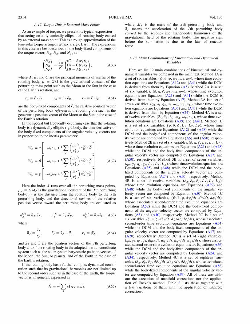
2314 FUKUSHIMA Vol. 135
A.12. Torque Due to External Mass Points
As an example of torque, we present its typical expression—that acting on a dynamically ellipsoidal rotating body causedby an external mass point. This is a rough approximation of theluni-solar torque acting on a triaxial rigid Earth. The expressionsin this case are best described in the body-fixed components ofthe torque vector, NA, NB , and NC , as(
NA
NB
NC
)= 3µ
r5
((C − B)rBrC
(A − C)rCrA
(B − A)rArB
), (A60)
where A, B, and C are the principal moments of inertia of therotating body, µ = GM is the gravitational constant of theperturbing mass point such as the Moon or the Sun in the caseof the Earth’s rotation, and
rA ≡ r · eA, rB ≡ r · eB, rC ≡ r · eC (A61)
are the body-fixed components of r , the relative position vectorof the perturbing body referred to the rotating one such as thegeocentric position vector of the Moon or the Sun in the case ofthe Earth’s rotation.
In the special but frequently occurring case that the rotatingbody is a dynamically elliptic rigid body, the time derivative ofthe body-fixed components of the angular velocity vectors arein proportion to the inertia parameters:
WA = α
[−ωBωC + 3
∑J
(µJ
r3J
)n
(J )B n
(J )C
],
WB = β
[−ωCωA + 3
∑J
(µJ
r3J
)n
(J )C n
(J )A
],
WC = γ
[−ωAωB + 3
∑J
(µJ
r3J
)n
(J )A n
(J )B
].
(A62)
Here the index J runs over all the perturbing mass points,µJ ≡ GMJ is the gravitational constant of the J th perturbingbody, rJ is the distance from the rotating body to the J thperturbing body, and the directional cosines of the relativeposition vector toward the perturbing body are evaluated as
n(J )A ≡ nJ ·eA, n
(J )B ≡ nJ ·eB, n
(J )C ≡ nJ ·eC, (A63)
where
nJ ≡ rJ
rJ
, rJ ≡ xJ − x, rJ ≡ |rJ |, (A64)
and xJ and x are the position vectors of the J th perturbingbody and of the rotating body in the adopted inertial coordinatesystem such as the solar system barycentric position vectors ofthe Moon, the Sun, or planets, and of the Earth in the case ofthe Earth’s rotation.
If the rotating body has a further complex dynamical consti-tution such that its gravitational harmonics are not limited upto the second order such as in the case of the Earth, the torquevector is, in general, expressed as
N = −∑
J
MJ rJ × aJ , (A65)
where MJ is the mass of the J th perturbing body andaJ means the acceleration of the J th perturbing bodycaused by the second- and higher-order harmonics of thegravitational field of the rotating body. The negative signbefore the summation is due to the law of reactionforce.
A.13. Main Combinations of Kinematical and DynamicalVariables
Here we list 12 main combinations of kinematical and dy-namical variables we compared in the main text. Method 1A isa set of six variables, (ψ, θ, φ, ωA, ωB, ωC), whose time evolu-tion equations are Equations (A12) and (A41) while the DCMis derived from them by Equation (A5). Method 2A is a setof six variables, (ξ, η, ζ, ωA, ωB, ωC), whose time evolutionequations are Equations (A21) and (A41) while the DCM isderived from them by Equation (A17). Method 3A is a set ofseven variables, (q0, q1, q2, q3, ωA, ωB, ωC), whose time evolu-tion equations are Equations (A35) and (A41) while the DCMis derived from them by Equation (A24). Method 4A is a setof twelve variables, (eA, eB, eC, ωA, ωB, ωC), whose time evo-lution equations are Equations (A39) and (A41). Method 1Bis a set of six variables, (ψ, θ, φ, LX,LY , LZ), whose timeevolution equations are Equations (A12) and (A48) while theDCM and the body-fixed components of the angular veloc-ity vector are computed by Equations (A5) and (A50), respec-tively. Method 2B is a set of six variables, (ξ, η, ζ, LX,LY , LZ),whose time evolution equations are Equations (A21) and (A48)while the DCM and the body-fixed components of the an-gular velocity vector are computed by Equations (A17) and(A50), respectively. Method 3B is a set of seven variables,(q0, q1, q2, q3, LX,LY , LZ), whose time evolution equations areEquations (A35) and (A48) while the DCM and the body-fixed components of the angular velocity vector are com-puted by Equations (A24) and (A50), respectively. Method4B is a set of twelve variables, (eA, eB, eC, LX,LY , LZ),whose time evolution equations are Equations (A39) and(A48) while the body-fixed components of the angular ve-locity vector are computed by Equation (A50). Method 1Cis a set of six variables, (ψ, θ, φ, dψ/dt, dθ/dt, dφ/dt),whose associated second-order time evolution equations areEquation (A52) while the DCM and the body-fixed compo-nents of the angular velocity vector are computed by Equa-tions (A5) and (A10), respectively. Method 2C is a set ofsix variables, (ξ, η, ζ, dξ/dt, dη/dt, dζ/dt), whose associatedsecond-order time evolution equations are Equations (A54)while the DCM and the body-fixed components of the an-gular velocity vector are computed by Equations (A17) and(A20), respectively. Method 3C is a set of eight variables,(q0, q1, q2, q3, dq0/dt, dq1/dt, dq2/dt, dq3/dt), whose associ-ated second-order time evolution equations are Equations (A56)while the DCM and the body-fixed components of the an-gular velocity vector are computed by Equations (A24) and(A34), respectively. Method 4C is a set of eighteen vari-ables, (eA, eB, eC, deA/dt, deB/dt, deC/dt), whose associatedsecond-order time evolution equations are Equations (A58)while the body-fixed components of the angular velocity vec-tor are computed by Equation (A59). All of these are with-out the execution of manifold corrections nor the applica-tion of Encke’s method. Table 2 lists these together witha few variations of them with the application of manifoldcorrections.
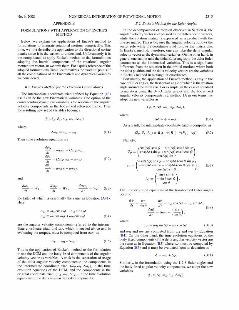
No. 6, 2008 NUMERICAL INTEGRATION OF ROTATIONAL MOTION 2315
APPENDIX B
FORMULATIONS WITH APPLICATION OF ENCKE’SMETHOD
Below, we explain the applications of Encke’s method toformulations to integrate rotational motions numerically. Thistime, we first describe the application to the directional cosinematrix since it is the easiest to understand. Unfortunately it istoo complicated to apply Encke’s method to the formulationsadopting the inertial components of the rotational angularmomentum vector, so we omit them. For a quick reference of theadopted formulations, Table 3 summarizes the essential points ofall the combinations of the kinematical and dynamical variableswe considered.
B.1. Encke’s Method for the Direction Cosine Matrix
The intermediate coordinate triad defined by Equation (10)itself can be the new kinematical variables. One option of thecorresponding dynamical variables is the residual of the angularvelocity components in the body-fixed reference frame. Thusthe resulting new set of variables becomes
(eD, eE, eC, ωA, ωB, ∆ωC)
where∆ωC ≡ ωC − ω0. (B1)
Their time evolution equations are
deD
dt= ωEeC − (∆ωC)eE,
deE
dt= (∆ωC)eD − ωDeC,
deC
dt= ωDeE − ωEeD
(B2)
and
dωA
dt= WA,
dωB
dt= WB,
d∆ωC
dt= WC, (B3)
the latter of which is essentially the same as Equation (A41).Here
ωD ≡ ωA cos ω0t − ωB sin ω0t,
ωE ≡ ωA sin ω0t + ωB cos ω0t (B4)
are the angular velocity components referred to the interme-diate coordinate triad, and ωC , which is needed above and inevaluating the torques, must be computed from ∆ωC as
ωC = ω0 + ∆ωC. (B5)
This is the application of Encke’s method to the formulationto use the DCM and the body-fixed components of the angularvelocity vector as variables. A trick is the separation of usageof the delta angular velocity components: the components inthe intermediate coordinate triad, (ωD,ωE,∆ωC), in the timeevolution equations of the DCM, and the components in theoriginal coordinate triad, (ωA,ωB, ∆ωC), in the time evolutionequations of the delta angular velocity components.
B.2. Encke’s Method for the Euler Angles
In the decomposition of rotation observed in Section 4, theangular velocity vector is expressed as the difference in vectors,while the rotation matrix is expressed as a product with theinverse matrix. This is because the angular velocity follows thevector rule while the coordinate triad follows the matrix one.In Encke’s method, therefore, one can take the delta angularvelocity vector as the dynamical variables. On the other hand, ingeneral one cannot take the delta Euler angles or the delta Eulerparameters as the kinematical variables. This is a significantdifference from the situation in the orbital motions where boththe delta position and the delta velocity vectors are the variablesin Encke’s method in rectangular coordinates.
Fortunately, the application of Encke’s method is easy in thecase of Euler angles, the first or last angle of which is the rotationangle around the third axis. For example, in the case of standardformulation using the 3-1-3 Euler angles and the body-fixedangular velocity components, i.e. method 1A in our terms, weadopt the new variables as
(ψ, θ, ∆φ,ωA, ωB, ∆ωC),
where∆φ ≡ φ − ω0t. (B6)
As a result, the intermediate coordinate triad is computed as
(eD, eE, eC) = R3(−ψ)R1(−θ )R3(−∆φ). (B7)
Namely,
eD =(
cos(∆φ) cos ψ − sin(∆φ) cos θ sin ψcos(∆φ) sin ψ + sin(∆φ) cos θ cos ψ
sin(∆φ) sin θ
),
eE =(−sin(∆φ) cos ψ − cos(∆φ) cos θ sin ψ
−sin(∆φ) sin ψ + cos(∆φ) cos θ cos ψcos(∆φ) sin θ
),
eC =(
sin θ sin ψ−sin θ cos ψ
cos θ
).
(B8)
The time evolution equations of the transformed Euler anglesbecome
dψ
dt= ωF
sin θ,
dθ
dt= ωD cos ∆φ − ωE sin ∆φ,
d∆φ
dt= ∆ωC −
( ωF
tan θ
),
(B9)
whereωF ≡ ωD sin ∆φ + ωE cos ∆φ, (B10)
and ωD and ωE are computed from ωA and ωB by Equation(B4). On the other hand, the time evolution equations of thebody-fixed components of the delta angular velocity vector arethe same as in Equation (B3) where ωC must be computed byEquation (B5) and φ must be evaluated from its deviation as
φ = ω0t + ∆φ. (B11)
Similarly, in the formulation using the 1-2-3 Euler angles andthe body-fixed angular velocity components, we adopt the newvariables
(ξ, η, ∆ζ, ωA, ωB, ∆ωC),
2316 FUKUSHIMA Vol. 135
where∆ζ ≡ ζ − ω0t. (B12)
See Appendix A.3 for the details of the symbols used. This time,the intermediate coordinate triad is defined in a matrix form as
(eD, eE, eC) = R1(−ξ )R2(−η)R3(−∆ζ ), (B13)
and written explicitly as
eD =(
cos(∆ζ ) cos ηsin(∆ζ ) cos ξ + cos(∆ζ ) sin η sin ξsin(∆ζ ) sin ξ − cos(∆ζ ) sin η cos ξ
),
eE =( −sin(∆ζ ) cos η
cos(∆ζ ) cos ξ − sin(∆ζ ) sin η sin ξcos(∆ζ ) sin ξ + sin(∆ζ ) sin η cos ξ
),
eC =(
sin η−cos η sin ξcos η cos ξ
).
(B14)
The time evolution equations of the delta Euler angles become
dξ
dt= ωG
cos η,
dη
dt= ωD sin ∆ζ + ωE cos ∆ζ,
d∆ζ
dt= ∆ωC − ωG tan η,
(B15)
whereωG ≡ ωD cos ∆ζ − ωE sin ∆ζ. (B16)
In the above, ωD and ωE are computed from ωA and ωB byEquation (B4) and
ζ = ω0t + ∆ζ. (B17)
B.3. Encke’s Method for the Euler Parameters
In contrast, the application of Encke’s method to formulationsusing the Euler parameters is complicated. In fact, we adopt anew set of variables including the new Euler parameters:
(p0, p1, p2, p3, ωA, ωB, ∆ωC),
where the new Euler parameters are defined such that theintermediate coordinate triad is expressed in the same manneras the original coordinate triad is expressed by the original Eulerparameters in Equation (A24):
eD =⎛⎝p2
0 + p21 − p2
2 − p23
2(p0p3 + p1p2)2(p1p3 − p0p2)
⎞⎠ ,
eE =⎛⎝ 2(p1p2 − p0p3)
p20 − p2
1 + p22 − p2
32(p0p1 + p2p3)
⎞⎠ , (B18)
eC =⎛⎝ 2(p0p2 + p1p3)
2(p2p3 − p0p1)p2
0 − p21 − p2
2 + p23
⎞⎠ .
The time evolution equations of the new Euler parameters areobtained as
dp0
dt= 1
2(−p1ωD − p2ωE − p3∆ωC),
dp1
dt= 1
2(+p0ωD − p3ωE + p2∆ωC),
dp2
dt= 1
2(+p3ωD + p0ωE − p1∆ωC),
dp3
dt= 1
2(−p2ωD + p1ωE + p0∆ωC),
(B19)
where ωD and ωE are computed from ωA and ωB byEquation (B4). Again the time evolution equations of ωA, ωB ,and ∆ωC are the same as in Equation (B3), where ωC must becomputed by Equation (B5). The constraint condition becomes
3∑j=0
p2j = 1, (B20)
and the associated renormalization is
pj → pj ≡ pj√∑3i=0 p2
i
. (B21)
B.4. Encke’s Method for Second-Order Ordinary DifferentialEquations of the Kinematical Variables
Encke’s method is also applicable to the formulations usingthe kinematical variables and their time derivatives as variablesto be integrated. For example, in the case of the 3-1-3 Eulerangles, we adopt the new variables(
ψ, θ, ∆φ,dψ
dt,dθ
dt,d∆φ
dt
).
First the intermediate coordinate triad is computed byEquation (B8) and the body-fixed components of the delta an-gular velocity vector, ωA, ωB , and ∆ωC , are evaluated as
ωA =(
dψ
dt
)sin θ sin φ +
(dθ
dt
)cos φ,
ωB =(
dψ
dt
)sin θ cos φ −
(dθ
dt
)sin φ, (B22)
∆ωC =(
dψ
dt
)cos θ +
(d∆φ
dt
).
These will be needed in calculating WA, WB , and WC . Then thesecond-order ordinary differential equations of the 3-1-3 Eulerangles are obtained as
d2ψ
dt2 = WF
sin θ,
d2θ
dt2 = WA cos φ − WB sin φ −(
ω0 +d∆φ
dt
) (dψ
dt
)sin θ,
d2∆φ
dt2 = WC −(
WF
tan θ
)+
(dθ
dt
) (dψ
dt
)sin θ,
(B23)
where WF is given as
WF = WA sin φ + WB cos φ +
(dθ
dt
)
×[ω0 +
(d∆φ
dt
)−
(dψ
dt
)cos θ
]. (B24)
In the above, ωC and φ must be computed by Equations (B5)and (B11), respectively.
Similarly, Encke’s method for the formulation using the 1-2-3Euler angles is described by the new variables(
ξ, η, ∆ζ,dξ
dt,dη
dt,d∆ζ
dt
).
No. 6, 2008 NUMERICAL INTEGRATION OF ROTATIONAL MOTION 2317
This time, the time evolution equations of the delta Euler anglesbecome
d2ξ
dt2 = WG
cos η,
d2η
dt2 = WA sin ζ + WB cos ζ +
(ω0 +
d∆ζ
dt
) (dξ
dt
)cos η,
d2∆ζ
dt2 = WC − WG tan η −(
dη
dt
) (dξ
dt
)cos η,
(B25)
where WG is given as
WG = WA cos ζ − WB sin ζ −(
dη
dt
)
×[ω0 +
(d∆ζ
dt
)−
(dξ
dt
)sin η
]. (B26)
The intermediate coordinate triad is computed byEquation (B14), and ωA, ωB , and ∆ωC contained in the ex-pressions of WA, WB , and WC are evaluated by
ωA =(
dξ
dt
)cos η cos ζ +
(dη
dt
)sin ζ,
ωB = −(
dξ
dt
)cos η sin ζ +
(dη
dt
)cos ζ,
∆ωC =(
dξ
dt
)sin η +
(d∆ζ
dt
),
(B27)
where ζ must be computed from Equation (B17).In the case of the Euler parameters, the new variables are(
p0, p1, p2, p3,dp0
dt,dp1
dt,dp2
dt,dp3
dt
).
The second-order ordinary differential equations of the newEuler parameters are
d2p0
dt2 = −[
(∆ ω)2
4
]p0 +
1
2(−p1WD − p2WE − p3WC),
d2p1
dt2 = −[
(∆ ω)2
4
]p1 +
1
2(+p0WD − p3WE + p2WC),
d2p2
dt2 = −[
(∆ ω)2
4
]p2 +
1
2(+p3WD + p0WE − p1WC),
d2p3
dt2 = −[
(∆ ω)2
4
]p3 +
1
2(−p2WD + p1WE + p0WC),
(B28)
where
(∆ ω)2 ≡ ω2A + ω2
B + (∆ωC)2 = ω2D + ω2
E + (∆ωC)2, (B29)
and
WD ≡ WA cos ω0t − WB sin ω0t,WE ≡ WA sin ω0t + WB cos ω0t.
(B30)
Also ωD , ωE , and ∆ωC are evaluated by
ωD = 2[−p1
(dp0
dt
)+ p0
(dp1
dt
)+ p3
(dp2
dt
)− p2
(dp3
dt
)],
ωE = 2[−p2
(dp0
dt
)− p3
(dp1
dt
)+ p0
(dp2
dt
)+ p1
(dp3
dt
)],
∆ωC = 2[−p3
(dp0
dt
)+ p2
(dp1
dt
)− p1
(dp2
dt
)+ p0
(dp3
dt
)].
(B31)
Once these are obtained, the body-fixed components, ωA, ωB ,and ωC , are easily evaluated from them as
ωA = ωD cos ω0t + ωE sin ω0t,
ωB = −ωD sin ω0t + ωE cos ω0t,
ωC = ω0 + ∆ωC.
(B32)
By using them, we can evaluate the expressions of WA, WB , andWC required. Also the intermediate coordinate triad is computedby Equation (B18). This time, the constraints are Equation (B20)and
3∑j=0
pj
(dpj
dt
)= 0. (B33)
Therefore, the manifold correction becomes the renormalizationgiven in Equation (B21) first and then the orthogonalization:
dpj
dt→
(dpj
dt
)≡ dpj
dt−
[3∑
i=0
pi
(dpi
dt
)]pj . (B34)
Finally, the new variables of Encke’s method for the case ofthe DCM are (
eD, eE, eC,deD
dt,deE
dt,deC
dt
).
The associated second-order ordinary differential equations are
d2eD
dt2 = − [ω2
E + (∆ωC)2] eD + (ωAωB − WC)eE
+ [(∆ωC)ωA + WE] eC,
d2eE
dt2 = (ωDωE + WC)eD − [(∆ωC)2 + ω2
A
]eE
+ [ωE(∆ωC) − WD]eC,
d2eC
dt2 = [(∆ωC)ωA − WB ] eD + [ωB(∆ωC) + WA] eE
− (ω2
A + ω2B
) eC, (B35)
where ωA, ωB , and ∆ωC are calculated as
ωD = eE ·(
deC
dt
)= −eC ·
(deE
dt
),
ωE = eC ·(
deD
dt
)= −eD ·
(deC
dt
), (B36)
∆ωC = eD ·(
deE
dt
)= −eE ·
(deD
dt
).
APPENDIX C
ANALYTICAL SOLUTION OF TORQUE-FREE ROTATION
Most standard textbooks in classical mechanics or in celestialmechanics do not display the analytical solution of torque-free rotation to the full extent. This is probably because theexpression of the solution is mathematically too complicated.Some sources in the literature illustrate only the solution ofthe dynamical variables such as the body-fixed components ofthe angular velocity vector, which are expressed in terms ofJacobi’s elliptic functions. Even academic articles rarely providethe full components of the kinematical variables, especially
2318 FUKUSHIMA Vol. 135
that of the rotation angle. An exception is Whittaker (1947).From the numerical viewpoint, however, its description usingthe logarithm of a function of elliptic theta functions of complexarguments may be too difficult to understand and evaluateefficiently.
Of course, this can be simply expressed by using the in-complete elliptic integral of the third kind (Kinoshita 1992).However, his expressions of the solution are based on the3-1-3 Euler angles, which are inappropriate when the magni-tude of the initial polar motion is small, as we encounter inmany practical applications, as seen in the main text. This issimilar to the phenomenon of small divisors we face in describ-ing the Keplerian orbits for the cases of nearly circular orbitsand/or orbits with small inclination.
Therefore, we provide here expressions of the solution basedon the second kind of Euler angles, namely the Euler angleswhose indices of the first and the third angles are different fromeach other. We describe the Euler angles in a coordinate systemwhose Z-axis is in parallel with the rotational angular momen-tum vector, L, which is conserved in the case of torque-freerotations. We express L in polar coordinates, namely its magni-tude and two angles referred to an inertial coordinate system. Asa result, the variables we deal with are the combination of thetotal angular momentum and the five angles: two for specifyingthe direction of L and the three Euler angles describing the ro-tation from an intermediate inertial reference frame associatedwith L and the body-fixed coordinate triad.
For the convenience of the reader, we present all the pos-sible cases of solutions as well as some hints to numericallyevaluate the aforementioned special functions appearing in theexpressions. Below, we provide the expression of the solution ofthe DCM and the body-fixed components of the angular veloc-ity vector only. This is because the other kinematical variablessuch as the 3-1-3 Euler angles, the 1-2-3 Euler angles, or theEuler parameters can be obtained from the DCM by their inverserelations, Equations (A6), (A18), or (A25), respectively.
C.1. Classification of Expressions of the Solution
The analytical solution of torque-free rotation is categorizedinto three cases except for a trivial one where A = B = C,which will be discussed in the next subsection. The classificationis according to the numerical value of a non-negative constantof motion, k, named as the modulus of elliptic functions. Morespecifically, the possible domain of k is 0 k ∞, which isdivided into three regions by a separatrix, k = 1: (1) 0 k < 1,(2) k = 1, and (3) 1 < k ∞. Physically speaking, the solutionis (1) averagely a uniform rotation around the C-axis in the firstcase, (2) asymptotic to a uniform rotation around the B-axis inthe second case, and (3) averagely a uniform rotation around theA-axis in the last case.
The C-axis is the axis of maximum moment of inertia. Ifwe assume that the rotating body has an ellipsoidal shape and auniform density, then this axis corresponds to the shortest axis ofthe ellipsoid. Thus, it is sometimes simply called the short axis.On the other hand, the A-axis is the axis of minimum moment ofinertia, which is named the long axis. Also the B-axis is calledthe middle axis. Therefore, we name the above three categoriesthe short, the middle, and the long axis modes, respectively.This manner of classification resembles that of Kepler orbits,the cases of elliptic, parabolic, and hyperbolic orbits accordingto the value of orbital eccentricity, 0 e < 1, e = 1, and1 < e ∞.
C.2. Case of a Dynamical Sphere
First of all, we consider the simplest case where A = B = Cand a = b = c. In this case, the expression of the solution is welldescribed by the combination of the 1-2-3 Euler angles and theinertial components of the rotational angular momentum vector,(ξ, η, ζ, LX,LY , LZ). The expressions of the solution are
ξ = ξ0, η = η0, ζ = ζ0 + cL0(t − t0),
LX = LX0, LY = LY0, LZ = LZ0,(C1)
where the suffix 0 means the values at the epoch t0 and
L0 ≡√
L2X0 + L2
Y0 + L2Z0. (C2)
Namely, the solution is a uniform rotation around the initialrotation axis.
C.3. Short Axis Mode
Next, consider the short axis mode where 0 k < 1. As willbe seen below, this condition is assured when A B < C,i.e. a b > c. The expression of the solution of theshort axis mode is best described in terms of the 1-2-3-2-1convention of modification of the Andoyer canonical variables,(L,w, v, z, y, x). This is because the first three of them areconstants of motion and only one of the remaining three, z, iscirculating.
The definitions of these variables except z are such that theinertial and body-fixed components of the rotational angular mo-mentum vector are expressed in the manner of polar coordinatesas
L ≡(
LX
LY
LZ
)= L
(sin v
cos v sin wcos v cos w
),
(LA
LB
LC
)= L
(sin y
cos y sin xcos y cos x
),
(C3)
while z is defined such that the DCM is computed as the productof five fundamental rotation matrices in the 1-2-3-2-1 manneras
R = R1(+w)R2(−v)R3(−z)R2(+y)R1(−x). (C4)
Note the signs of the five angles. In the torque-free rotation, thefirst three variables are constants of motion:
L = L0, w = w0, v = v0. (C5)
The time evolution equations of the remaining three variablesare
dx
dt= L[(a − b) sin2 x + (a − c) cos2 x] sin y,
dy
dt= −L(b − c) sin x cos x cos y,
dz
dt= L(b sin2 x + c cos2 x).
(C6)
Their solutions become
x = tan−1
[√1 + f (tan y0)
(sn(u, k)
dn(u, k)
)],
y = sin−1[(sin y0)cn(u,k)],
z = z0 + aL0(t − t0) −(√
1 + f
cos y0
)pn(u, − tan2 y0, k),
(C7)
No. 6, 2008 NUMERICAL INTEGRATION OF ROTATIONAL MOTION 2319
wherek ≡ (
√f ) tan y0 (C8)
is the modulus of the elliptic functions,
f ≡ a − b
b − c 0 (C9)
is a triaxiality parameter,
u ≡ n(t − t0) (C10)
is the argument of elliptic functions, and
n ≡ L0(a − c) cos y0√1 + f
(C11)
is the speed of the argument of elliptic functions, which reducesto the mean speed of the precessional motion in the limit of adynamically oblate spheroid, A = B and a = b. Thus we maycall n the mean precession.
In the above, sn(u, k), cn(u, k), and dn(u, k) are Jacobi’s sine,cosine, and delta amplitude functions, respectively, and
pn(u, n, k) ≡∫ u
0
dv
1 − nsn2(v, k)(C12)
is the incomplete elliptic integral of the third kind regarded as afunction of u, n, and k. Here we denote the parameter of ellipticintegral by n, which is sometimes expressed as α2 in some of theliterature. Later we comment on how to compute these specialfunctions numerically.
The subscript 0 means the value at the epoch t = t0, which isdefined as the time when x = 0 and y = y0 0. Therefore thesix constants of torque-free rotational motion become L0, w0,v0, z0, y0, and t0. The condition 0 k < 1 implies the possibledomain of y0 as
0 y0 < tan−1
(1√f
) π
2. (C13)
This assures that cos y0 is nonzero and tan y0 is finite. Note theproperty of Jacobi’s elliptic functions,
|sn(u, k)| 1,
|cn(u, k)| 1,
dn(u, k) =√
1 − k2sn2(u, k),
(C14)
for the real values of u and k satisfying the condition 0 k < 1.Thus we learn that the above expressions of the solution are welldefined and the possible domains of x and y are limited as
|x| x1 ≡ tan−1
[(√1 + f
1 − f tan2 y0
)tan y0
]<
π
2,
|y| y0 <π
2.
(C15)
This means that the angles x and y are librating. Also, t0 can besaid to be the time when y is a maximum.
The expressions of the solution of x and y above lead to theexpressions of the solution of the body-fixed components of theangular momentum and the angular velocity vectors:(
LA
LB
LC
)=
(AωA
BωB
CωC
)= L0
⎛⎝ (sin y0)cn(u, k)√
1 + f (sin y0) sn(u, k)(cos y0)dn(u, k)
⎞⎠ . (C16)
As a result, the rotational energy, T , which is conserved underno torque, is expressed as
T ≡ aL2A + bL2
B + cL2C
2= L2
0(a sin2 y0 + c cos2 y0)
2. (C17)
Below, we describe two special sub-cases of this mode.
C.3.1. Case of a Dynamically Oblate Spheroid
One special case is that of an oblately spheroidal body whenA = B < C and a = b > c. In this case, f = k = 0 while0 y0 < π/2. As a result, the mean precession becomes
n = L0(a − c) cos y0. (C18)
Also Jacobi’s elliptic functions reduce to trigonometric ones andunity:
sn(u,0) = sin u, cn(u,0) = cos u, dn(u, 0) = 1.(C19)
Further, the incomplete elliptic integral of the third kind be-comes
pn(u,−tan2y0, 0) = (cos y0)
[u + tan−1
2 sin2
(y0
2
)
×(
sin u cos u
(cos y0) cos2 u + sin2 u
)]. (C20)
Therefore, the expression of the solution reduces to the simpleform
x = tan−1[(tan y0) sin u], y = sin−1[(sin y0) cos u],
z = z0 + nC(t − t0) (C21)
− tan−1
[2 sin2
(y0
2
)(sin u cos u
(cos y0) cos2 u + sin2 u
)],
wherenC ≡ L0[a − (a − c) cos y0] (C22)
is the mean rotational speed, i.e. the mean speed of angle variablez, in the oblate spheroid case.
C.3.2. Case of Minimum Energy
Another special case occurs when y0 = 0 while f = 0 ingeneral. In this case, k = 0. As a result, the mean precessionbecomes
n = L0
√(a − c)(b − c), (C23)
and the incomplete elliptic integral of the third kind reduces tou itself:
pn(u, 0, 0) = u. (C24)
Thus, the expression of the solution becomes very simple:
x = y = 0, z = z0 + cL0(t − t0). (C25)
This means a uniform rotation around the C-axis. Under thecondition L0 is constant, the rotational energy reaches itsminimum
T = cL20
2. (C26)
Thus, we name this the minimum energy case.
2320 FUKUSHIMA Vol. 135
C.4. Long Axis Mode
Third, let us consider the long axis mode where 1 < k ∞.This condition is assured when A < B C, i.e. a > b c.The expression of the solution of the long axis mode is easilyobtained from that of the short axis mode by the exchange ofindices/notations:
(1, A, a,X, x) ←→ (3, C, c, Z, z). (C27)
In fact, the expression is best described in terms of the3-2-1-2-3 convention of modification of the Andoyer canonicalvariables, (L, v∗, w∗, x∗, y∗, z∗). This time, only one circulat-ing angle variable becomes x∗, the rotation angle around theA-axis.
The definitions of these angles are similar to those of the1-2-3-2-1 ones:
L ≡(
LX
LY
LZ
)= L
(cos w∗ cos v∗cos w∗ sin v∗
sin w∗
),
(LA
LB
LC
)= L
(cos y∗ cos z∗cos y∗ sin z∗
sin y∗
), (C28)
and
R = R3(+v∗)R2(−w∗)R1(−x∗)R2(+y∗)R3(−z∗). (C29)
Again the first three variables are constants of motion:
L = L0, v∗ = v∗0 , w∗ = w∗
0 . (C30)
The other variables are expressed as functions of time:
z∗ = tan−1
[√1 + f ∗(tan y∗
0 )
(sn(u∗, k∗)
dn(u∗, k∗)
)],
y∗ = sin−1[(sin y∗0 )cn(u∗, k∗)]
x∗ = x∗0 + cL0(t − t0) +
(√1 + f ∗
cos y∗0
)pn(u∗, tan2 y∗
0 , k∗).
(C31)
Here
u∗ ≡ n∗(t − t0), n∗ ≡ L0(a − c) cos y∗0√
1 + f ∗ ,
k∗ ≡ (√
f ∗) tan y∗0 f ∗ ≡ b − c
a − b 0.
(C32)
The duality relations between the quantities of the short axismode and those of the long axis mode, namely those withoutand those with asterisks, are
n∗ = kn, u∗ = ku, k∗ = 1
k, f ∗ = 1
f, y∗
0 = π
2− y0.
(C33)Again the subscript 0 means values at the epoch t = t0. Thistime the epoch is defined as the time when z∗ = 0 and y∗ reachesits maximum value, y∗
0 . The condition of the long axis mode,1 < k ∞, is translated into that of k∗ as 0 k∗ < 1. Thisimplies that y∗
0 is in the range
0 y∗0 < tan−1
(1√f ∗
) π
2. (C34)
The expressions of the body-fixed components of the angularmomentum and the angular velocity vectors are
(LA
LB
LC
)=
(AωA
BωB
CωC
)= L0
⎛⎝ (cos y∗
0 ) dn(u∗,k∗)√1 + f ∗(sin y∗
0 ) sn(u∗,k∗)
(sin y∗0 ) cn(u∗, k∗)
⎞⎠ .
(C35)Consequently, the rotational energy is expressed as
T = L20(a cos2 y∗
0 + c sin2 y∗0 )
2. (C36)
Below, we describe a couple of special sub-cases of this mode.
C.4.1. Case of a Dynamically Prolate Spheroid
One special case is that of a prolate spheroidal body whenA < B = C and a > b = c. In this case, f ∗ = k∗ = 0 while0 y∗
0 < π/2. As a result, the dual mean precession becomes
n∗ = L0(a − c) cos y∗0 . (C37)
The expression of the solution reduces to the simple form
z∗ = tan−1[(tan y∗0 ) sin u∗], y∗ = sin−1[(sin y∗
0 ) cos u∗],
x∗ = x∗0 + nA(t − t0) (C38)
+ tan−1
[2 sin2
(y∗
0
2
) (sin u∗ cos u∗
(cos y∗0 ) cos2 u∗ + sin2 u∗
)],
wherenA ≡ L0[c + (a − c) cos y∗
0 ] (C39)
is the mean rotational speed, i.e. the mean speed of angle variablex∗, in the prolate spheroidal case.
C.4.2. Case of Maximum Energy
Another special case occurs when y∗0 = 0 while f ∗ = 0
in general. In this case, k∗ = 0. As a result, the dual meanprecession becomes
n∗ = L0
√(a − c)(a − b), (C40)
and the incomplete elliptic integral of the third kind reduces tou∗ itself:
pn(u∗, 0, 0) = u∗. (C41)
Thus the expression of the solution becomes very simple:
z∗ = y∗ = 0, x∗ = x∗0 + aL0(t − t0). (C42)
This is nothing but a uniform rotation around the A-axis. Inthis case, the rotational energy reaches its maximum under thecondition L0 is constant:
T = aL20
2. (C43)
Therefore, we name it the maximum energy case.
C.5. Middle Axis Mode
The last mode is when k = 1. In this case, the solution isasymptotic to a uniform rotation around the B-axis both in thelimits of the infinite past and the infinite future. Therefore we
No. 6, 2008 NUMERICAL INTEGRATION OF ROTATIONAL MOTION 2321
name this the middle axis mode. This time the expression ofthe solution can be well described by either the 1-2-3-2-1 or3-2-1-2-3 conventions. Here we adopt the former style.
In this mode, f is assured to be positive and y0 becomes afunction of f :
sin y0 = 1√1 + f
, cos y0 =√
f
1 + f, tan y0 = 1√
f,
(C44)since
k ≡ (√
f ) tan y0 = 1. (C45)
As a result, the mean precession becomes
n = L0
√(a − b)(b − c). (C46)
Also Jacobi’s elliptic functions reduce to hyperbolic ones:
sn(u,1) = tanh u, cn(u,1) = dn(u,1) = 1
cosh u. (C47)
Further, the incomplete elliptic integral of the third kind be-comes
pn
(u,
−1
f,1
)= f
1 + f
[u +
1√f
tan−1
(tanh u√
f
)]. (C48)
Therefore the solution becomes
x = tan−1
[(√1 + f
f
)sinh u
],
y = sin−1
[1
(√
1 + f ) cosh u
],
z = z0 + bL0(t − t0) − tan−1
(tanh u√
f
).
(C49)
The expressions of the body-fixed components of the angularmomentum and the angular velocity vectors are(
LA
LB
LC
)=
(AωA
BωB
CωC
)= L0
(√
1 + f ) cosh u
⎛⎝ 1
sinh u√f
⎞⎠ . (C50)
As a result, the rotational energy, T , is expressed as
T = bL20
2. (C51)
In the limit t → ±∞, the solution becomes as simple as
x → ±(π
2
), y → 0,
z → z0 ∓ y0 + bL0(t − t0).
(C52)
In this limit case, the body-fixed angular velocity componentstend to be constant:
ωA → 0, ωB → ±bL0, ωC → 0. (C53)
This manifests that the asymptotic motions are uniform rotationsaround the B-axis.
C.6. Hints on Numerical Computation of Elliptic Functionsand Integrals
As seen in the above subsections, we need four kinds of spe-cial functions to express analytically the torque-free solution of
rotational motion. They are Jacobi’s elliptic functions, sn(u, k),cn(u, k), and dn(u, k), and the incomplete elliptic integral ofthe third kind expressed in terms of Jacobi’s elliptic functions,pn(u, n, k), which we call the pi amplitude function for short.The numerical computation of these functions occupies the keyrole in describing torque-free rotations in the same sense thatthe solving procedure of Kepler’s equation is important in dis-cussing two-body problems. Therefore, below, we present somepractical hints to compute them precisely and efficiently.
The numerical computation of the first three elliptic functionsis rather an easy task. The standard procedure to evaluate themnumerically is the use of descending and ascending Landentransformations. Since the core part of the transformations,the famous arithmetic–geometric mean, is common to all threefunctions, the computing routine is usually designed to evaluatethem simultaneously for the same argument and modulus. Anexample of its numerical algorithm is given in the routinesncndn in Section 6.12.1 of Press et al. (2007). Unfortunately,the implemented code loses its efficiency if the magnitude ofthe first argument, |u|, is large, say more than thousands of theperiod of elliptic functions. This is the same situation as wherewe face a loss of precision in evaluating trigonometric functionsof large arguments. To avoid this problem, we recommend,before calling the routine sncndn, to take the modulus of uwith respect to the period as
u → u ≡ mod(u, 4K(k)), (C54)
where
K(k) ≡∫ π/2
0
dθ√1 − k2 sin2 θ
(C55)
is the complete elliptic integral of the first kind, which is afunction of the modulus k only.
On the other hand, the numerical evaluation of the pi ampli-tude function is a complicated process. Assume the availabilityof a numerical procedure to compute the incomplete ellipticintegral of the third kind in the Legendre form,
Π (ϕ, n, k) ≡∫ ϕ
0
dθ
(1 − n sin2 θ )√
1 − k2 sin2 θ. (C56)
Usually the computing routine itself is constructed under theassumption that the first argument, ϕ, is an angle variable,namely assuming that it is of periodicity 2π . We must transformit into the pi amplitude function, the first argument of which, u,has the modulus 4K(k). A way to realize it is the use of Jacobi’samplitude function, am(u, k), as
pn(u, n, k) = Π (am(u, k),n, k). (C57)
Unfortunately, there is no fast numerical way to evaluatethe amplitude function directly. The procedures using Landentransformations require the evaluation of trigonometric andinverse trigonometric functions frequently. This is significantlyslow. Also no fast rational expression using theta functionsis found for the amplitude function. This is different fromthe situation in sn(u, k), cn(u, k), and dn(u, k). Meanwhile,its Fourier expansion series converges slowly. Therefore, wecompute it from the numerical values of Jacobi’s ellipticfunctions mentioned above as
am(u, k) = 2π
[u
4K(k)
]Gauss
+ am(u, k), (C58)
where [ ]Gauss denotes the Gauss integer truncation function, uis the modulated value of u given above, and

2322 FUKUSHIMA Vol. 135
am(u, k) ≡ atan2(sn(u, k),cn(u, k)). (C59)
If 0 k < 1, Jacobi’s three elliptic functions can be expressedas trigonometric functions of the amplitude function:
sn(u, k) = sin ϕ,
cn(u, k) = cos ϕ,
dn(u,k) =√
1 − k2 sin2 ϕ,
(C60)
whereϕ ≡ am(u,k). (C61)
This is the reason why the first two of them are named thesine amplitude and the cosine amplitude, respectively; the lastis called the delta amplitude function.
Since the pi amplitude function contains a secular component,it is wise to separate its linear and periodic parts in the numericalevaluation:
pn(u, n, k) = 4Π (n, k)
[u
4K(k)
]Gauss
+ Π (am(u, k), n, k),
(C62)
where
Π (n,k) ≡∫ π/2
0
dθ
(1 − n sin2 θ )√
1 − k2 sin2 θ(C63)
is the complete elliptic integral of the third kind.Finally we mention how to calculate the incomplete and
complete elliptic integrals. There are two predominant methodsof evaluating them: (i) those using the aforementioned pairof Landen transformations or their modification known asthe Bartkey transformation (Burlisch 1969a, 1969b), and (ii)Carlson’s method briefly introduced in Section 6.12 of Presset al. (2007).
We prefer the former because if we introduce a singlefunction called the incomplete elliptic integral in general form(Fukushima and Ishizaki 1994),
G(ϕ, nc,mc, a, b) ≡∫ ϕ
0
(a cos2 θ + b sin2 θ ) dθ
(cos2 θ + nc sin2 θ )√
cos2 θ + mc sin2 θ,
(C64)then the incomplete and complete elliptic integrals of all threekinds, namely (1) the incomplete elliptic integral of the firstkind,
F (ϕ, k) ≡∫ ϕ
0
dθ√1 − k2 sin2 θ
, (C65)
(2) the incomplete elliptic integral of the second kind,
E(ϕ, k) ≡∫ ϕ
0(√
1 − k2 sin2 θ ) dθ, (C66)
and (3) the complete elliptic integral of the second kind,
E(k) ≡∫ π/2
0(√
1 − k2 sin2 θ ) dθ, (C67)
as well as K(k), Π (ϕ,n,k), and Π (n,k), already appeared above,can be evaluated by the function as
F (ϕ, k) = G(ϕ, 1, 1 − k2, 1, 1), (C68)
K(k) = G(π
2, 1, 1 − k2, 1, 1
), (C69)
E(ϕ, k) = G(ϕ, 1, 1 − k2, 1, 1 − k2), (C70)
E(k) = G(π
2, 1, 1 − k2, 1, 1 − k2
), (C71)
Π (ϕ, n, k) = G(ϕ, 1 − n, 1 − k2, 1, 1), (C72)
Π (n, k) = G(π
2, 1 − n, 1 − k2, 1, 1
). (C73)
Frequently we require elliptic functions and incomplete ellip-tic integrals for different values of u while fixing k and/or n.From the practical viewpoint, therefore, we recommend design-ing their computing routines so as to store the calculated valuesof the complete elliptic integrals such as K(k) or Π (n, k) andreuse them unless k and/or n change(s). Available from the au-thor is a package of the Fortran codes to compute all the above-mentioned functions, sn(u, k), cn(u, k), dn(u, k), am(u, k), andpi(u, n, k), taking all these hints into account.
REFERENCES
Altman, S. P. 1972, Celest. Mech., 6, 425Arribas, M., Elipe, A., & Palacios, M. 2006, Celest. Mech. Dyn. Astron.,
96, 239Beutler, G. 2005, Methods of Celestial Mechanics Vol. I and II (Berlin: Springer)Brouwer, D., & Clemence, G. M. 1961, Methods of Celestial Mechanics (New
York: Academic)Brumberg, V. A., & Ivanova, T. V. 2007, Celest. Mech. Dyn. Astron., 97, 189Burlisch, R. 1969a, Numer. Math., 13, 266Burlisch, R. 1969b, Numer. Math., 13, 305Cappallo, R. J., King, R. W., Counselmann, C. C., & I. I., III, Shapiro
1981, Moon and Planets, 24, 281Dehant, V., et al. 1999, Celest. Mech. Dyn. Astron., 72, 245Deprit, A. 1994, in Dynamics and Astrometry of Natural and Artificial Celestial
Bodies, Proc. Conf. on Astrometry and Celestial Mechanics, Poznan,Poland, September 13–17, 1993, ed. K. Kurzynska, et al., (Poznan, Poland:Astronomical Observatory, A. Mickiewicz Univ.), 159
Fukushima, T. 1993, Celest. Mech. Dyn. Astron., 60, 57Fukushima, T. 1996, AJ, 112, 1263Fukushima, T. 2003a, AJ, 126, 494Fukushima, T. 2003b, AJ, 126, 1097Fukushima, T. 2003c, AJ, 126, 3138Fukushima, T. 2005, AJ, 129, 2496Fukushima, T. 2007a, AJ, 133, 1Fukushima, T. 2007b, AJ, 133, 2815Fukushima, T., & Ishizaki, H. 1994, Celest. Mech. Dyn. Astron., 59, 149Goldstein, H. 1980, Classical Mechanics (2nd ed.; Reading, MA: Addison-
Wesley)Goldstein, H., Poole, C. P., & Safko, J. L. 2002, Classical Mechanics (3rd ed.;
Reading, MA: Addison-Wesley)Hairer, E., Lubich, C., & Wanner, G. 1999, Geometric Numerical Integration
(Berlin: Springer)Hilton, J. L., et al. 2006, Celest. Mech. Dyn. Astron., 94, 351Huang, T.-Y., & Innanen, 1983, AJ, 88, 870Hughes, P. C. 1986, Spacecraft Attitude Dynamics (New York: Wiley)Kinoshita, H. 1972, PASJ, 24, 423Kinoshita, H. 1992, Celest. Mech. Dyn. Astron., 53, 365Krasinsky, G. A. 2006, Celest. Mech. Dyn. Astron., 96, 169MacMillan, W. D. 1936, Dynamics of Rigid Bodies (New York: Dover),
(reprinted 1960)Murison, M. A. 1989, AJ, 97, 1496Nacozy, P. E. 1971, Astrophys. Space Sci., 14, 40Press W. H., Teukolsky S. A., Vetterling W. T., & Flannery B. P. 2007,
Numerical Recipes: The Art of Scientific Computing (3rd ed.; Cambridge,MA: Cambridge Univ. Press)
Whittaker, E. T. 1947, A Treatise on the Analytical Dynamics of Particles andRigid Bodies (4th ed.; Cambridge, MA: Cambridge Univ. Press)