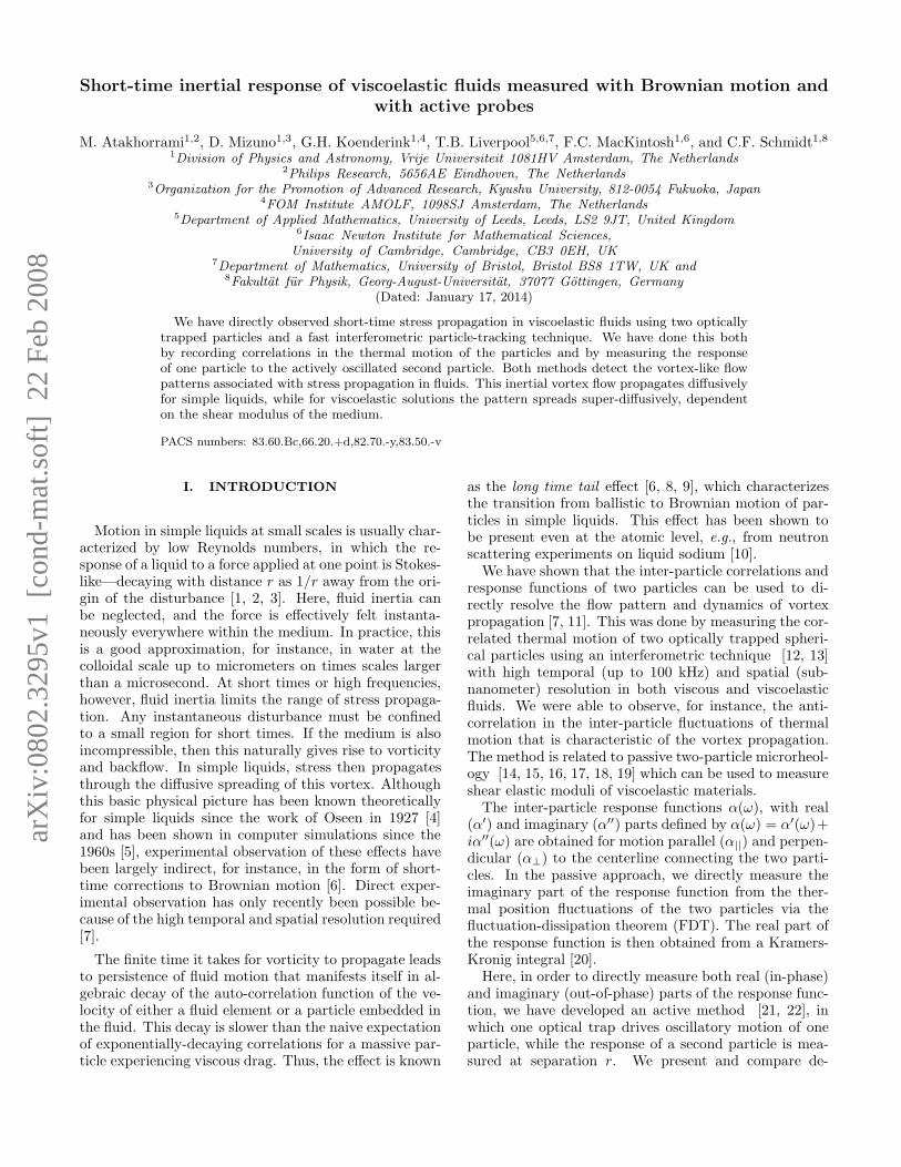
arX

iv:0

802.

3295

v1 [

cond

-mat

.sof

t] 2

2 Fe

b 20

08

Short-time inertial response of viscoelastic fluids measured with Brownian motion and

with active probes

M. Atakhorrami1,2, D. Mizuno1,3, G.H. Koenderink1,4, T.B. Liverpool5,6,7, F.C. MacKintosh1,6, and C.F. Schmidt1,81Division of Physics and Astronomy, Vrije Universiteit 1081HV Amsterdam, The Netherlands

2Philips Research, 5656AE Eindhoven, The Netherlands3Organization for the Promotion of Advanced Research, Kyushu University, 812-0054 Fukuoka, Japan

4FOM Institute AMOLF, 1098SJ Amsterdam, The Netherlands5Department of Applied Mathematics, University of Leeds, Leeds, LS2 9JT, United Kingdom

6Isaac Newton Institute for Mathematical Sciences,

University of Cambridge, Cambridge, CB3 0EH, UK7Department of Mathematics, University of Bristol, Bristol BS8 1TW, UK and

8Fakultat fur Physik, Georg-August-Universitat, 37077 Gottingen, Germany

(Dated: January 17, 2014)

We have directly observed short-time stress propagation in viscoelastic fluids using two opticallytrapped particles and a fast interferometric particle-tracking technique. We have done this bothby recording correlations in the thermal motion of the particles and by measuring the responseof one particle to the actively oscillated second particle. Both methods detect the vortex-like flowpatterns associated with stress propagation in fluids. This inertial vortex flow propagates diffusivelyfor simple liquids, while for viscoelastic solutions the pattern spreads super-diffusively, dependenton the shear modulus of the medium.

PACS numbers: 83.60.Bc,66.20.+d,82.70.-y,83.50.-v

I. INTRODUCTION

Motion in simple liquids at small scales is usually char-acterized by low Reynolds numbers, in which the re-sponse of a liquid to a force applied at one point is Stokes-like—decaying with distance r as 1/r away from the ori-gin of the disturbance [1, 2, 3]. Here, fluid inertia canbe neglected, and the force is effectively felt instanta-neously everywhere within the medium. In practice, thisis a good approximation, for instance, in water at thecolloidal scale up to micrometers on times scales largerthan a microsecond. At short times or high frequencies,however, fluid inertia limits the range of stress propaga-tion. Any instantaneous disturbance must be confinedto a small region for short times. If the medium is alsoincompressible, then this naturally gives rise to vorticityand backflow. In simple liquids, stress then propagatesthrough the diffusive spreading of this vortex. Althoughthis basic physical picture has been known theoreticallyfor simple liquids since the work of Oseen in 1927 [4]and has been shown in computer simulations since the1960s [5], experimental observation of these effects havebeen largely indirect, for instance, in the form of short-time corrections to Brownian motion [6]. Direct exper-imental observation has only recently been possible be-cause of the high temporal and spatial resolution required[7].

The finite time it takes for vorticity to propagate leadsto persistence of fluid motion that manifests itself in al-gebraic decay of the auto-correlation function of the ve-locity of either a fluid element or a particle embedded inthe fluid. This decay is slower than the naive expectationof exponentially-decaying correlations for a massive par-ticle experiencing viscous drag. Thus, the effect is known

as the long time tail effect [6, 8, 9], which characterizesthe transition from ballistic to Brownian motion of par-ticles in simple liquids. This effect has been shown tobe present even at the atomic level, e.g., from neutronscattering experiments on liquid sodium [10].

We have shown that the inter-particle correlations andresponse functions of two particles can be used to di-rectly resolve the flow pattern and dynamics of vortexpropagation [7, 11]. This was done by measuring the cor-related thermal motion of two optically trapped spheri-cal particles using an interferometric technique [12, 13]with high temporal (up to 100 kHz) and spatial (sub-nanometer) resolution in both viscous and viscoelasticfluids. We were able to observe, for instance, the anti-correlation in the inter-particle fluctuations of thermalmotion that is characteristic of the vortex propagation.The method is related to passive two-particle microrheol-ogy [14, 15, 16, 17, 18, 19] which can be used to measureshear elastic moduli of viscoelastic materials.

The inter-particle response functions α(ω), with real(α′) and imaginary (α′′) parts defined by α(ω) = α′(ω)+iα′′(ω) are obtained for motion parallel (α||) and perpen-dicular (α⊥) to the centerline connecting the two parti-cles. In the passive approach, we directly measure theimaginary part of the response function from the ther-mal position fluctuations of the two particles via thefluctuation-dissipation theorem (FDT). The real part ofthe response function is then obtained from a Kramers-Kronig integral [20].

Here, in order to directly measure both real (in-phase)and imaginary (out-of-phase) parts of the response func-tion, we have developed an active method [21, 22], inwhich one optical trap drives oscillatory motion of oneparticle, while the response of a second particle is mea-sured at separation r. We present and compare de-

2

tailed experimental results of both passive and activeapproaches. We also present a theoretical derivation ofthe predicted response functions and corresponding alge-braic decay of the velocity autocorrelation functions forviscoelastic fluids.

The outline of the paper is as follows. In section II,we present the theoretical analysis. In section III, wepresent the materials and methods of sample prepara-tion, as well as the experimental techniques for the pas-sive and active measurements of the response functions.In section IV we describe our methods of data analysisused for the results presented in section V. In the resultssection V, we first compare the data for simple liquidswith the dynamic Oseen tensor, which demonstrates thediffusive propagation of the vortex flow. We then presentour results and comparison with theory for viscoelasticsolutions, including the evidence for superdiffusive stresspropagation. Finally, we conclude with a discussion (sec-tion VI), also mentioning implications of our results formicrorheology in general.

II. THEORY AND BACKGROUND

Newtonian liquids are described by the Navier-Stokesequation, which is non-linear. The non-linearity, how-ever, can usually be neglected either for small distancesor for low velocities [1, 2]. This is the so-called lowReynolds number regime, since the relative importanceof non-linearities is characterized by the Reynolds num-ber Re = ULρ

η , where U , L, ρ, and η are, respectively,

the characteristic velocity and length scales, the density,and the viscosity. For steady flow, this regime can alsobe thought of as the non-inertial regime, in which stresspropagates instantaneously and, for instance, the veloc-ity response at a distance r from a point force variesas 1/r [1, 2, 3]. Such Stokes flow accurately describesthe motion of micron-size objects in water on time scaleslonger than a few microseconds.

Even at low Reynolds number, however, there are re-maining consequences of fluid inertia for non-stationaryflows [3]. This unsteady Stokes approximation is de-scribed by the linearized Navier-Stokes equation:

ρ∂

∂t~v = η∇2~v − ~∇P + ~f, (1)

where ~v is the velocity field, P is the pressure that en-

forces the incompressibility of the liquid and ~f is the forcedensity applied to the fluid. By taking the curl of this

equation we observe that the vorticity ~Ω = ~∇×~v satisfiesthe diffusion equation with diffusion constant ν = η/ρ.

As noted above, the short-time response of a liquidto a point force generates a vortex. The propagation ofstress away from the point disturbance is diffusive: aftera time t, this vortex expands away from the point forceto a size of order δ ∼

√

ηt/ρ. In the wake of this movingvortex is the usual Stokes flow that corresponds to a 1/r

dependence of the velocity field. For an oscillatory distur-bance at frequency ω, the propagation of vorticity definesa penetration depth δ ∼

√

η/(ωρ) [1]. Stress effectivelypropagates instantaneously on length scales shorter thanthis.

This picture generalizes to the case of homogenousviscoelastic media characterized by an isotropic, time-dependent shear modulus G(t) [23], although the prop-agation of stress generally becomes super-diffusive [11].We further assume that the medium is incompressible,which is a particularly good approximation for polymersolutions such as those considered here, at least at highfrequencies [20, 24, 25]. The deformation of the mediumis characterized by a local displacement field ~u(~r, t), andthe viscoelastic analogue of the Navier-Stokes equation(1) is:

ρ∂2

∂t2~u(~r, t) = ~∇ · σ↔(~r, t) − ~∇P + ~f(~r, t) , (2)

where

σ↔

(~r, t) = 2

∫ t

−∞

dt′G(t− t′)γ↔

(~r, t′) (3)

is the local stress tensor and

γ↔

=1

2

[

~∇~u+(

~∇~u)†]

(4)

is the local deformation tensor. Incompressibility corre-

sponds to the constraint ~∇ · ~u = 0Equations (2,3) can be simplified by a decomposition

of the force density and deformation into Fourier com-ponents. Taking spatio-temporal Fourier Transforms de-fined as

~u(~k, ω) =

∫

d3r

∫ ∞

−∞

dt ei(ωt−~k·~r)~u(~r, t), (5)

and defining the complex modulus

G⋆(ω) ≡ G′(ω) + iG′′(ω) =

∫ ∞

0

dteiωtG(t), (6)

we can eliminate the pressure by imposing incompress-ibility in Eqs. (2,3). This leads to

~u(~k, ω) =

(

1 − kk

G⋆(ω)k2 − ρω2

)

· ~f(~k, ω) , (7)

where k = ~k/|k|. We invert this Fourier transform toobtain the displacement response function due to a pointforce applied at the origin.

A. Response functions

For a point force ~f at the origin, the linear responseof the medium at ~r is given by a tensor αij , where

3

ui(~r, ω) = αij(~r, ω)fj(~0, ω). Here, αij = α′ij + iα′′

ij is, ingeneral, complex. Given our assumptions of rotationaland translational symmetry, there are only two distinctcomponents of the response. These are (1) a parallel re-sponse that is given by a displacement field ~u parallel

to both ~f and ~r, and (2) a perpendicular response given

by ~u parallel to ~f and perpendicular to ~r. The parallelresponse function α‖, for instance, is obtained from theinverse Fourier transform of Eq. (7) [11].

The response functions for general G⋆(ω) are given by

α‖ (r, ω) = α′‖ + i α′′

‖ =1

4πG⋆(ω)rχ‖

(

r√κ)

, (8)

and

α⊥ (r, ω) = α′⊥ + i α′′

⊥ =1

8πG⋆(ω)rχ⊥

(

r√κ)

, (9)

where κ = ρω2/G⋆(ω) is complex and

χ‖ (x) =2

x2

[

(1 − ix) eix − 1]

, (10)

and

χ⊥ (x) =2

x2

[

1 +(

x2 − 1 + ix)

eix]

. (11)

The magnitude of κ defines the inverse (viscoelastic) pen-etration depth δ.

1. Simple liquids

For a simple liquid, G⋆(ω) = −i ωη and κ = iρω/η.The velocity response of the liquid is then characterizedby

− iωα‖ (r, ω) = ωα′′‖ − i ωα′

‖ =1

4πηrχ‖

(

r

√

ρω

2η

)

, (12)

and

− iωα⊥ (r, ω) = ωα′′⊥ − i ωα′

⊥ =1

8πηrχ⊥

(

r

√

ρω

2η

)

,

(13)where

χ′‖ (x) =

[(1 + x) sinx− x cosx] e−x

x2, (14)

χ′′‖ (x) =

1 − [(1 + x) cosx+ x sinx] e−x

x2, (15)

χ′⊥ (x) =

[(

x+ 2x2)

cosx− (1 + x) sinx]

e−x

x2, (16)

χ′′⊥ (x) =

[(

x+ 2x2)

sinx+ (1 + x) cosx]

e−x − 1

x2.

(17)

Thus, for instance, the in-phase and out-of-phase velocityresponse in the parallel direction are given by ωα′′ =

14πηr χ

′‖ and −ωα′ = 1

4πηr χ′′‖ .

0 1 2 3 4 5 6 7 8-0.4

-0.2

0.0

0.2

0.4

0.6

0.8

1.0

r = 10.3µm

α"||

α'||

a

||

||

4π r

η ω

α

r / δv

0 1 2 3 4 5 6 7 8

-0.4

-0.2

0.0

0.2

0.4

0.6

0.8

1.0

r = 11.3µm

⊥α"

⊥

α'⊥

b

⊥8

π r

η ω

α

r / δv

FIG. 1: Comparison of theoretical and experimentally mea-sured response functions for a simple liquid. The predictionsof the normalized velocity field from the dynamic Oseen tensorin Eqs. (12,13) are shown as black and gray lines. Normal-ized complex inter-particle response functions between twoprobe particles (silica beads, R = 0.58 µm) measured withthe active microrheology method in water: (a) 4πrηωα|| inthe parallel direction and (b) 8πrηωα⊥ in the perpendiculardirection, plotted versus the ratio of the separation distancer (fixed for a given bead pair, r = 11.3 µm for parallel, andr = 10.3 µm for perpendicular) to the frequency-dependentviscous penetration depth δv. Both real (filled symbols) andimaginary parts (open symbols) are shown, for both paral-lel and perpendicular directions. These results are comparedwith the theory for η = 0.97 mPa s and ρ = 1000 kg m−3.There is good agreement with no free parameters.

We have written the response functions in Eqs. (8, 9) ina form in which the noninertial limits (x→ 0) are simple:χ‖,⊥ → 1. Thus, for a simple liquid in the limit x → 0,Eqs. (12, 13) reduce to the (time-independent) Oseentensor [2, 4]. For finite x, these response functions givethe dynamic Oseen tensor [4, 26], which are shown as thesolid lines in Fig. 1, where for small r/δ the parallel andperpendicular velocity response (i.e., −iωα‖,⊥) approach

4

14πηr and 1

8πηr for a unit force at the origin. These then

decay for r & δ. The region of negative response in theperpendicular case corresponds to the back-flow of thevortex.

The response functions above represent the ensemble-average displacements due to forces acting in themedium. These response functions also govern the equi-librium thermal fluctuations and the correlated fluctua-tions from point to point within the medium. The rela-tionship between thermal fluctuations and response is de-scribed by the Fluctuation-Dissipation theorem. Specif-ically, for points separated by a distance r along the xdirection,

C‖,⊥(r, ω) =2kBT

ωα′′‖,⊥(r, ω), (18)

where

C‖(r, ω) =

∫ ∞

−∞

dteiωt〈ux(0, 0)ux(r, t)〉 (19)

and

C⊥(r, ω) =

∫ ∞

−∞

dteiωt〈uy(0, 0)uy(r, t)〉. (20)

2. Polymer solutions

An experimentally pertinent illustration is given by thehigh frequency complex shear modulus of a polymer so-lution,

G⋆(ω) = −iωη + g(−iω)z = |G|e−iψ (21)

which has both solvent and polymer contributions. Forthe Rouse model of flexible polymers z = 1/2 [27], whilefor semiflexible polymers z = 3/4 [20, 28, 29]. The lattercase is shown as the solid lines in Fig. 2. We see thatthe oscillatory or anti-correlated response becomes morepronounced in viscoelastic materials.

The magnitude of the complex modulus is given by

|G| =

√

(gωz)2

+ (ωη)2

+ 2ωz+1ηg sin (πz/2), (22)

while its phase is given by

sinψ =(ωη + gωz sin (πz/2))

|G| (23)

and

cosψ =gωz cos (πz/2)

|G| . (24)

It is also useful to have the following expressions for thehalf-phase-angles

sinψ

2=

√

1

2

(

1 − gωz cos (πz/2)

|G|

)

(25)

cosψ

2=

√

1

2

(

1 +gωz cos (πz/2)

|G|

)

. (26)

We define the real parameter β = r√

ρω2/|G| and use the definitions, Eqns. (10,11) to obtain the following compactexpressions for the response functions (α⊥, α‖) which can be expanded using the compound angle formulae and thedefinitions above. The real and imaginary parts of the parallel response are given by

4π|G|rα′‖(r, ω) =

2

β2

e−β sin ψ

2

[

cos

(

β cosψ

2

)

+ β sin

(

ψ

2+ β cos

ψ

2

)]

− 1

(27)

and

4π|G|rα′′‖(r, ω) =

2

β2e−β sin ψ

2

sin

(

β cosψ

2

)

− β cos

(

ψ

2+ β cos

ψ

2

)

, (28)

while the corresponding expressions for the perpendicular response are given by

8π|G|rα′⊥(r, ω) =

2

β2

1 − e−β sin ψ

2

[

cos

(

β cosψ

2

)

+ β sin

(

ψ

2+ β cos

ψ

2

)

− β2 cos

(

ψ + β cosψ

2

)]

(29)

and

8π|G|rα′′⊥(r, ω) =

2

β2e−β sin ψ

2

− sin

(

β cosψ

2

)

+ β cos

(

ψ

2+ β cos

ψ

2

)

+ β2 sin

(

ψ + β cosψ

2

)

. (30)

The imaginary part of the response functions will be used to calculate the correlation functions, Eq. (18), used foranalysis of the passive experiments whilst the real part of the response functions will be used for comparison with theactive experiments.

5

We can simplify the expressions above in the limit that the polymer contribution to the viscoelasticity dominatesthe shear modulus. We then obtain the simple scaling form G⋆(ω) ≃ g(−iω)z[30] giving |G| = g |ω|z , ψ = πz/2.Further simplification of Eq. (18) using the expressions in Eqs. (30,28) and definitions in Eqs. (10,11) leads, e.g., to

C‖(r, ω) =kBT

2πω|G|r 2

β2e− sin( zπ4 )β

[(

1 + sin(

zπ4

)

β)

sin[

cos(

zπ4

)

β]

− cos(

zπ4

)

β cos[

cos(

zπ4

)

β]

]

, (31)

where β = r√

ρω2/|G| characterizes the overall decay of stress due to inertia. This decay corresponds to super-diffusive propagation of stress for viscoelastic media with G ∼ ωz and z < 1, since the response is limited to a spatialrange that grows with time as t(2−z)/2.

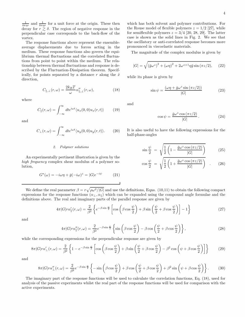
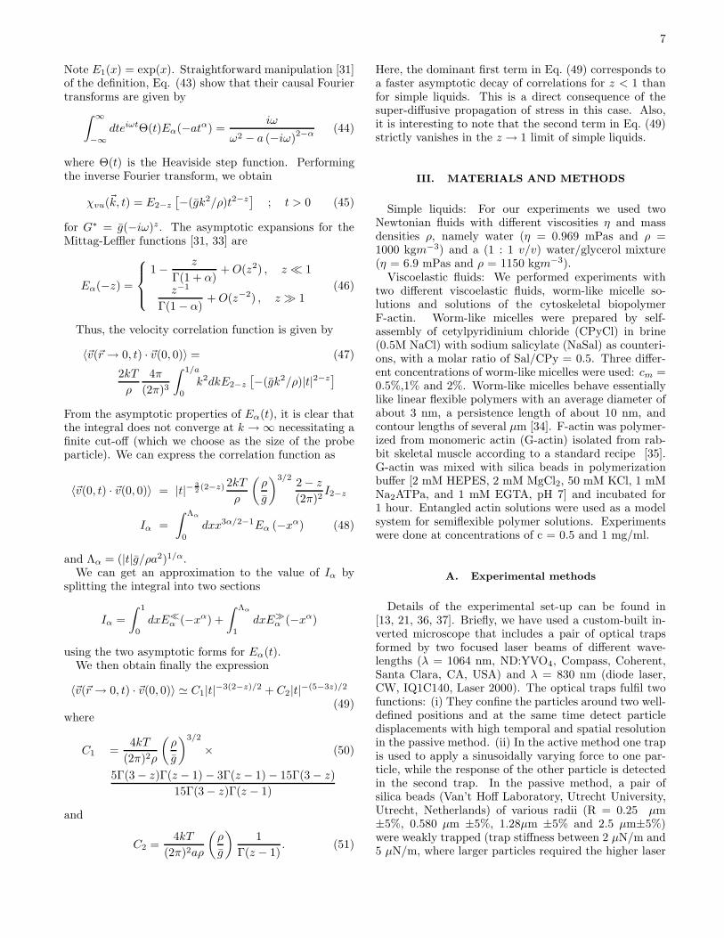
The resulting displacement field, exhibiting the vortexpattern, is shown in Fig. 3 for a point force at the ori-gin pointed along the x-axis. This flow pattern exhibitsspecific inversion symmetries: vx (vy) is symmetric (anti-symmetric) for either x→ −x or y → −y, as can be seenby the fact that the (linear) response must everywherereverse if the direction of the force is reversed.

B. Velocity autocorrelations and the long time tail

The self-sustaining back-flow represented in Fig. 3gives rise to long-lived correlations that, for instance, af-fect the crossover from ballistic to diffusive motion of aparticle in a liquid. For a simple liquid, the fluid velocity(auto)correlations 〈~v(0, t) · ~v(0, 0)〉 decay proportional to∼ |t|−3/2. This is known as the long time tail [5, 6, 8].For a viscoelastic fluid, stress propagation is faster thandiffusive, resulting in a more rapid decay of velocity cor-relations. The decay is, however, still algebraic.

1. Simple liquids

For a simple liquid, Eq. (1) means that

(

−iωρ+ ηk2)

vi =(

δij − kikj

)

fj (32)

for the Fourier transforms. This gives the response in

velocity vi to a force component fj that is (thermody-namically) conjugate to a displacement uj. We denotethis response function by χviuj , where

χviuj (~k, ω) =

(

δij − kikj

)

ηk2 − iωρ. (33)

The fluctuation-dissipation theorem then tells us that

χviuj (~r, t) = − 1

kT

d

dt〈vi(~r, t)uj(0, 0)〉, (34)

where this is valid only for t > 0 because of causalityin the response. The correlation function is, however,defined for both positive and negative times.

Due to translation invariance in time, the correlationfunction 〈vi(~r, t+ t′)uj(0, t

′)〉 must be independent of t′.

Thus,

0 =d

dt′〈vi(~r, t+ t′)uj(0, t

′)〉 (35)

= 〈vi(~r, t+ t′)uj(0, t′)〉 + 〈vi(~r, t+ t′)vj(0, t

′)〉,

which also means that

kTχviuj (~r, t)〉 = 〈vi(~r, t)vj(0, 0)〉.

Again, this is valid only for t > 0 because of causality inthe response. Ultimately, however, we are interested inthe autocorrelation function 〈~v · ~v〉 = 〈vivi〉, for r → 0above. In this case, the correlation function is manifestlysymmetric in t. Thus,

〈vi(~r → 0, t)vi(0, 0)〉 = kTχviui(~r → 0, |t|). (36)

We first calculate χviuj

(

~k, t)

, since the limit

χviuj (~r → 0, t) can be obtained from this simply by in-

tegrating over all ~k.

χviuj (~k, t) =

(

δij − kikj

)

∫

dω

2πe−iωt

1

ηk2 − iωρ

=

(

δij − kikj

)

−2πiρ

∫

e−iωtdω

ω + iνk2,

where ν = η/ρ. But, the last integral can only dependon the combination tνk2, since we can replace ω by ζνk2,where ζ is dimensionless. Specifically,

χviuj (~k, t) =

(

δij − kikj

)

−2πiρ

∫

e−iζνk2t dζ

ζ + i

=

(

δij − kikj

)

ρe−νk

2t (37)

for t > 0. Otherwise, the result is zero. This integral canbe done by integration along a closed contour containingthe real line in either the upper half-plane for t < 0, orthe lower half plane for t > 0.

Finally, to get the limit

χviui(~r → 0, t) (38)

6

0 1 2 3 4 5 6

-0.6

-0.4

-0.2

0.0

0.2

0.4

0.6

0.8

1.0

r =12.1 µm a

α"||

α'||

||

4π r

|G

| α

||

r / δve

0 2 4 6

-0.5

0.0

0.5

1.0

r =13.5 µm

α'⊥

α"⊥

b

⊥

8π r

|G

| α

⊥

r / δve

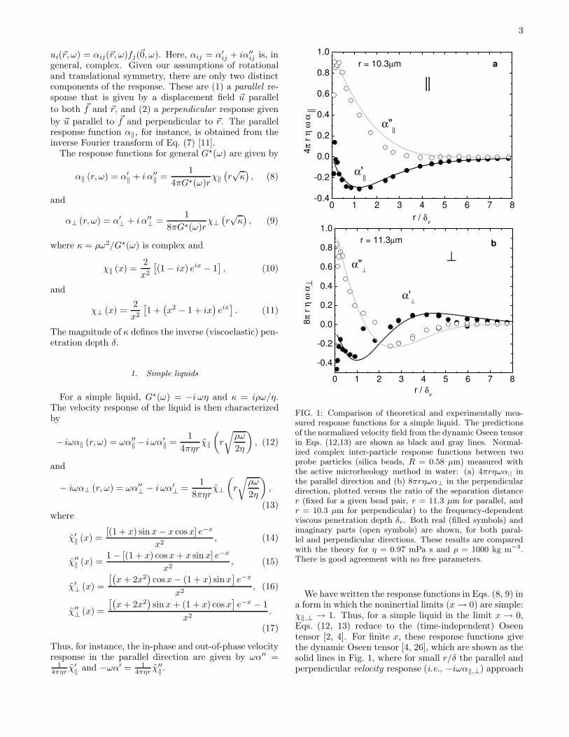
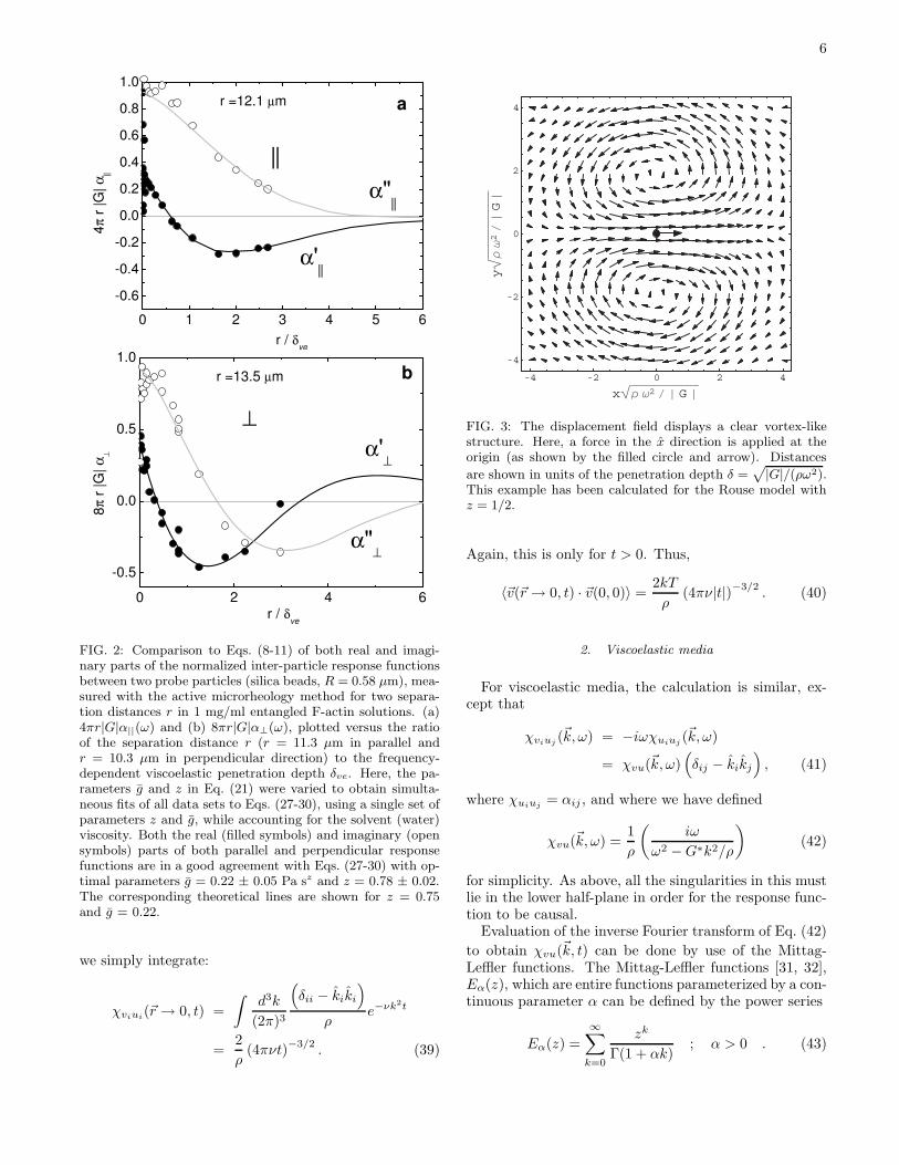
FIG. 2: Comparison to Eqs. (8-11) of both real and imagi-nary parts of the normalized inter-particle response functionsbetween two probe particles (silica beads, R = 0.58 µm), mea-sured with the active microrheology method for two separa-tion distances r in 1 mg/ml entangled F-actin solutions. (a)4πr|G|α||(ω) and (b) 8πr|G|α⊥(ω), plotted versus the ratioof the separation distance r (r = 11.3 µm in parallel andr = 10.3 µm in perpendicular direction) to the frequency-dependent viscoelastic penetration depth δve. Here, the pa-rameters g and z in Eq. (21) were varied to obtain simulta-neous fits of all data sets to Eqs. (27-30), using a single set ofparameters z and g, while accounting for the solvent (water)viscosity. Both the real (filled symbols) and imaginary (opensymbols) parts of both parallel and perpendicular responsefunctions are in a good agreement with Eqs. (27-30) with op-timal parameters g = 0.22 ± 0.05 Pa sz and z = 0.78 ± 0.02.The corresponding theoretical lines are shown for z = 0.75and g = 0.22.

we simply integrate:

χviui(~r → 0, t) =

∫

d3k

(2π)3

(

δii − kiki

)

ρe−νk

2t

=2

ρ(4πνt)

−3/2. (39)

-4 -2 0 2 4

xè!!!!!!!!!!!!!!!!!!!!!!!!ρ ω2 ê » G »

-4

-2

0

2

4

yè!!!!!!!!!!!!!!!!!!!!!!!!

ρω2ê»G»

FIG. 3: The displacement field displays a clear vortex-likestructure. Here, a force in the x direction is applied at theorigin (as shown by the filled circle and arrow). Distances

are shown in units of the penetration depth δ =p

|G|/(ρω2).This example has been calculated for the Rouse model withz = 1/2.

Again, this is only for t > 0. Thus,

〈~v(~r → 0, t) · ~v(0, 0)〉 =2kT

ρ(4πν|t|)−3/2

. (40)

2. Viscoelastic media

For viscoelastic media, the calculation is similar, ex-cept that

χviuj (~k, ω) = −iωχuiuj (~k, ω)

= χvu(~k, ω)(

δij − kikj

)

, (41)

where χuiuj = αij , and where we have defined

χvu(~k, ω) =1

ρ

(

iω

ω2 −G∗k2/ρ

)

(42)

for simplicity. As above, all the singularities in this mustlie in the lower half-plane in order for the response func-tion to be causal.

Evaluation of the inverse Fourier transform of Eq. (42)

to obtain χvu(~k, t) can be done by use of the Mittag-Leffler functions. The Mittag-Leffler functions [31, 32],Eα(z), which are entire functions parameterized by a con-tinuous parameter α can be defined by the power series

Eα(z) =

∞∑

k=0

zk

Γ(1 + αk); α > 0 . (43)

7

Note E1(x) = exp(x). Straightforward manipulation [31]of the definition, Eq. (43) show that their causal Fouriertransforms are given by

∫ ∞

−∞

dteiωtΘ(t)Eα(−atα) =iω

ω2 − a (−iω)2−α(44)

where Θ(t) is the Heaviside step function. Performingthe inverse Fourier transform, we obtain

χvu(~k, t) = E2−z

[

−(gk2/ρ)t2−z]

; t > 0 (45)

for G∗ = g(−iω)z. The asymptotic expansions for theMittag-Leffler functions [31, 33] are

Eα(−z) =

1 − z

Γ(1 + α)+O(z2) , z ≪ 1

z−1

Γ(1 − α)+O(z−2) , z ≫ 1

(46)

Thus, the velocity correlation function is given by

〈~v(~r → 0, t) · ~v(0, 0)〉 = (47)

2kT

ρ

4π

(2π)3

∫ 1/a

0

k2dkE2−z

[

−(gk2/ρ)|t|2−z]

From the asymptotic properties of Eα(t), it is clear thatthe integral does not converge at k → ∞ necessitating afinite cut-off (which we choose as the size of the probeparticle). We can express the correlation function as

〈~v(0, t) · ~v(0, 0)〉 = |t|− 3

2(2−z) 2kT

ρ

(

ρ

g

)3/22 − z

(2π)2I2−z

Iα =

∫ Λα

0

dxx3α/2−1Eα (−xα) (48)

and Λα = (|t|g/ρa2)1/α.We can get an approximation to the value of Iα by

splitting the integral into two sections

Iα =

∫ 1

0

dxE≪α (−xα) +

∫ Λα

1

dxE≫α (−xα)

using the two asymptotic forms for Eα(t).We then obtain finally the expression

〈~v(~r → 0, t) · ~v(0, 0)〉 ≃ C1|t|−3(2−z)/2 + C2|t|−(5−3z)/2

(49)where

C1 =4kT

(2π)2ρ

(

ρ

g

)3/2

× (50)

5Γ(3 − z)Γ(z − 1) − 3Γ(z − 1) − 15Γ(3 − z)

15Γ(3 − z)Γ(z − 1)

and

C2 =4kT

(2π)2aρ

(

ρ

g

)

1

Γ(z − 1). (51)

Here, the dominant first term in Eq. (49) corresponds toa faster asymptotic decay of correlations for z < 1 thanfor simple liquids. This is a direct consequence of thesuper-diffusive propagation of stress in this case. Also,it is interesting to note that the second term in Eq. (49)strictly vanishes in the z → 1 limit of simple liquids.

III. MATERIALS AND METHODS

Simple liquids: For our experiments we used twoNewtonian fluids with different viscosities η and massdensities ρ, namely water (η = 0.969 mPas and ρ =1000 kgm−3) and a (1 : 1 v/v) water/glycerol mixture(η = 6.9 mPas and ρ = 1150 kgm−3).

Viscoelastic fluids: We performed experiments withtwo different viscoelastic fluids, worm-like micelle so-lutions and solutions of the cytoskeletal biopolymerF-actin. Worm-like micelles were prepared by self-assembly of cetylpyridinium chloride (CPyCl) in brine(0.5M NaCl) with sodium salicylate (NaSal) as counteri-ons, with a molar ratio of Sal/CPy = 0.5. Three differ-ent concentrations of worm-like micelles were used: cm =0.5%,1% and 2%. Worm-like micelles behave essentiallylike linear flexible polymers with an average diameter ofabout 3 nm, a persistence length of about 10 nm, andcontour lengths of several µm [34]. F-actin was polymer-ized from monomeric actin (G-actin) isolated from rab-bit skeletal muscle according to a standard recipe [35].G-actin was mixed with silica beads in polymerizationbuffer [2 mM HEPES, 2 mM MgCl2, 50 mM KCl, 1 mMNa2ATPa, and 1 mM EGTA, pH 7] and incubated for1 hour. Entangled actin solutions were used as a modelsystem for semiflexible polymer solutions. Experimentswere done at concentrations of c = 0.5 and 1 mg/ml.

A. Experimental methods

Details of the experimental set-up can be found in[13, 21, 36, 37]. Briefly, we have used a custom-built in-verted microscope that includes a pair of optical trapsformed by two focused laser beams of different wave-lengths (λ = 1064 nm, ND:YVO4, Compass, Coherent,Santa Clara, CA, USA) and λ = 830 nm (diode laser,CW, IQ1C140, Laser 2000). The optical traps fulfil twofunctions: (i) They confine the particles around two well-defined positions and at the same time detect particledisplacements with high temporal and spatial resolutionin the passive method. (ii) In the active method one trapis used to apply a sinusoidally varying force to one par-ticle, while the response of the other particle is detectedin the second trap. In the passive method, a pair ofsilica beads (Van’t Hoff Laboratory, Utrecht University,Utrecht, Netherlands) of various radii (R = 0.25 µm±5%, 0.580 µm ±5%, 1.28µm ±5% and 2.5 µm±5%)were weakly trapped (trap stiffness between 2 µN/m and5 µN/m, where larger particles required the higher laser

8

intensities to avoid shot noise. Transmitted laser lightwas imaged onto two quadrant photo diodes, such thatparticle displacements and in the x and y directions weredetected interferometrically [12]. A specialized siliconPIN photodiode (YAG444-4A, Perkin Elmer, Vaudreuil,Canada), operated at a reverse bias of 110 V, was usedin order to extend the frequency range up to 100 kHz forthe 1064 nm laser [38]. The 830 nm laser was detectedby a standard silicon PIN photodiode operated at a re-verse bias of 15 V (Spot9-DMI, UDT, Hawthorne, CA).Amplified outputs were digitized at 195 kHz (A/D inter-face specs ) and further processed in Labview (NationalInstruments, Austin, TX, USA). Output voltages wereconverted to actual displacements using Lorentzian fitsto power spectral densities (PSD) as described in [39]. Inthe case of water, calibration was done on the beads thatwere used in the experiments, while for the viscoelasticsolutions and the more viscous liquid, calibrations weredone in water with beads from the same batch.

In the active method, the 1064 nm laser was usedto oscillate one particle, while the 830 nm laser wasused for detection of the second particle at a sep-aration distance r. The driving laser was deflectedthrough an Acousto-Optical Deflector (AOD) (TeO2,Model DTD 276HB6, IntraAction, Bellwood, Illinois),using a voltage-controlled oscillator (VCO) (DRF.40, AAOPTO-ELECTRONIC, Orsay, France). The force ap-plied to the driven particle was calibrated by measuringthe PSD of the Brownian motion of a particle of the samesize trapped in water with the same laser power [39].The output signal from the QPD detecting the secondlaser was fed into a lock-in amplifier (SR830, StanfordResearch Systems, Sunnyvale, CA, USA) to obtain am-plitude and phase of particle response. All experimentswere done in sample chambers made from a glass slideand a cover slip with about 140 µm inner height, with theparticles at at least 25 µm distance from both surfaces.The lab temperature was stabilized at T = 21.5 C.

IV. DATA ANALYSIS

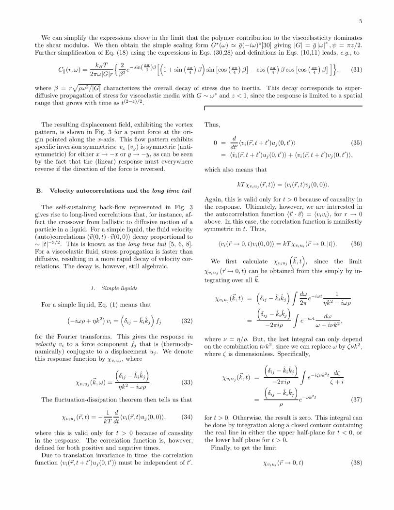
In both the active and passive methods we calculatethe linear complex response function α defined by u(ω) =α(ω)×F (ω), where F (ω) is the applied force. Linear re-sponse applies by definition in the passive method, and inthe active method the particle displacements u(ω) werekept sufficiently small. Again, we consider separatelyreal, α′(ω), and imaginary parts, α′′(ω), of the response.In all our experiments, as sketched in Fig. 4, the coordi-nate system was chosen in such a way that x is parallelto the line connecting the centers of the two particles (||)and y perpendicular (⊥)to that. The inter-particle re-sponse functions along these two directions were used todetermine the flow field.

The displacement u(1)x (ω) of particle 1 in the x di-

rection is related to the force F(2)x acting on particle

2 according to u(1)x (ω) = α||(ω) × F

(2)x (ω). Similarly,

x

y

z

FIG. 4: (Color online) Schematic sketch of the experiment.A pair of silica beads (radius R) is trapped by a pair of lasertraps at a separation distance r. In the passive method, theposition fluctuations of each particle in the x and y directionsare simultaneously detected with quadrant photodiodes andthe displacement cross-correlations are measured parallel andperpendicular to the line connecting the centers of the twobeads. In the active method, one of the beads is oscillatedby rapidly moving one laser trap either in x or in y directionand the resulting motion of the other particle is measured inx and in y direction. Laser intensity was adjusted to result inthe trap stiffness of typically between (2µN/m and 5µN/m)for passive measurements.

the perpendicular response function was derived from

u(1)y (ω) = α⊥(ω) × F

(2)y (ω). The single-particle re-

sponse functions for each x and y directions are de-

fined as u(1)x,y(ω) = αauto(ω) × F

(1)x (ω). For homoge-

neous, isotropic media, the two functions α||,⊥(ω) com-pletely characterize the linear response at any point inthe medium due to a force at another point. The dis-placement response functions α||,⊥(ω) determine bothposition and velocity response −iωα||,⊥(ω).

In the passive approach, the medium fluctuates inequilibrium, and the only forces on the particles arethermal/Brownian forces. Therefore the fluctuation-dissipation theorem (FDT) of statistical mechanics [40]relates the response of the medium to the displacementcorrelation functions. For two particles, these correla-tion functions are the cross-correlated displacement fluc-

tuations: 〈u(1)x (t)u

(2)x (0)〉 and 〈u(1)

y (t)u(2)y (0)〉. We used

Fast Fourier Transforms (FFT) to calculate displacementcross-correlation functions in frequency space and ob-tained the imaginary parts of the complex inter-particleresponse functions α′′

||,⊥(ω) via the FDT:

α′′||(ω) =

ω∫

〈u(1)x (t)u

(2)x (0)〉eiωtdt

2kT(52)

9

and

α′′⊥(ω) =

ω∫

〈u(1)y (t)u

(2)y (0)〉eiωtdt

2kT, (53)

where k is the Boltzman constant and T is the controlledlaboratory temperature. The real parts of inter-particleresponse functions α′

||,⊥(ω) were obtained by a Kramers-

Kronig integral:

α′||,⊥(ω) =

2

πP

∫ ∞

0

ζα′′||,⊥(ω)

ζ2 − ω2(54)

=2

π

∫ ∞

0

cos(tω)

∫ ∞

0

α′′||,⊥(ζ) sin(tζ)dζ,

where P denotes a principal-value integral [20]. The highfrequency cut-off of the Kramers-Kroning integral lim-its the frequency range of the calculated α′

||,⊥(ω) [13].

We also used the active method to obtain both real andimaginary parts of the response functions with 100 kHzbandwidth, as in Refs. [21, 37]. Here the lock-in am-plifier provides directly in-phase (real part) and out-of-phase (imaginary part) response of the second particle.The measurements were done over a grid of driving fre-quencies.

V. RESULTS

A. Simple liquids

In the low-frequency limit, where fluid inertia can beneglected, the inter-particle response functions are in-versely related to the shear modulus of the medium[20, 24, 41]. For a simple viscous fluid, the responsefunctions in this limit are given by:

α|| = 2α⊥ =i

4πrωη(55)

where r is the separation distance between the two par-ticles and η is the viscosity. These relations also shows(via the FDT) a 1/r dependence of the Fourier transformof the displacement cross-correlation functions:

S|| =

∫

〈u(1)x (t)u(2)

x (0)〉eiωtdt (56)

and

S⊥ =

∫

〈u(1)y (t)u(2)

y (0)〉eiωtdt (57)

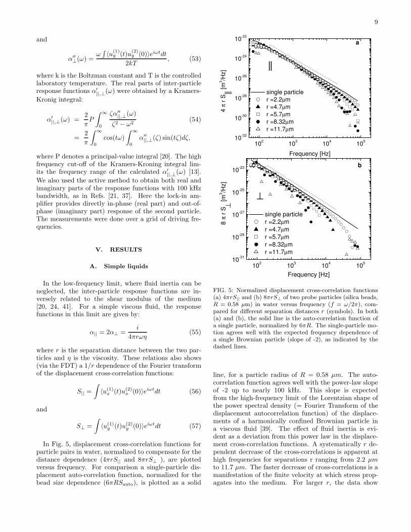
In Fig. 5, displacement cross-correlation functions forparticle pairs in water, normalized to compensate for thedistance dependence (4πrS|| and 8πrS⊥ ), are plottedversus frequency. For comparison a single-particle dis-placement auto-correlation function, normalized for thebead size dependence (6πRSauto), is plotted as a solid

102

103

104

105

10-32

1x10-30

1x10-28

10-26

1x10-24

10-22

-

a

||

||4

π r

S

[m

3/H

z]

Frequency [Hz]

single particle

r =2.2µm

r =4.7µm

r =5.7µm

r =8.32µm

r =11.7µm

102

103

104

105

10-31

1x10-29

10-27

10-25

1x10-23

-

b

⊥

⊥8

π r

S

[m

3/H

z]

Frequency [Hz]

single particle

r =2.2µm

r =4.7µm

r =5.7µm

r =8.32µm

r =11.7µm

FIG. 5: Normalized displacement cross-correlation functions(a) 4πrS|| and (b) 8πrS⊥ of two probe particles (silica beads,R = 0.58 µm) in water versus frequency (f = ω/2π), com-pared for different separation distances r (symbols). In both(a) and (b), the solid line is the auto-correlation function ofa single particle, normalized by 6πR. The single-particle mo-tion agrees well with the expected frequency dependence ofa single Brownian particle (slope of -2), as indicated by thedashed lines.

line, for a particle radius of R = 0.58 µm. The auto-correlation function agrees well with the power-law slopeof -2 up to nearly 100 kHz. This slope is expectedfrom the high-frequency limit of the Lorentzian shape ofthe power spectral density (= Fourier Transform of thedisplacement autocorrelation function) of the displace-ments of a harmonically confined Brownian particle ina viscous fluid [39]. The effect of fluid inertia is evi-dent as a deviation from this power law in the displace-ment cross-correlation functions. A systematically r de-pendent decrease of the cross-correlations is apparent athigh frequencies for separations r ranging from 2.2 µmto 11.7 µm. The faster decrease of cross-correlations is amanifestation of the finite velocity at which stress prop-agates into the medium. For larger r, the data show

10

that the decrease begins at a lower frequency, becauseit takes longer for stress to propagate further. A com-parison of Figs. 5a and b shows that the decrease ofthe cross-correlation is, at the same separation distance,more pronounced in the perpendicular channel than inthe parallel channel. This is due to the fact that in thevortex-like flow pattern of Fig. 3 there is a region of fluidmotion in the opposite direction to the applied force. Forr > 5 µm (open squares), the cross-correlations becomenegative in the observed frequency window (not shownin the log-log plot). At still higher frequencies, the dis-placement cross-correlation functions again become pos-itive (Fig. 5b), which is visible for the larger separations,r = 8.3 µm and r = 11.7 µm, consistent with the ex-pected oscillation in the displacement cross-correlationfunctions in the frequency domain. This effect becomesmore pronounced in viscoelastic media

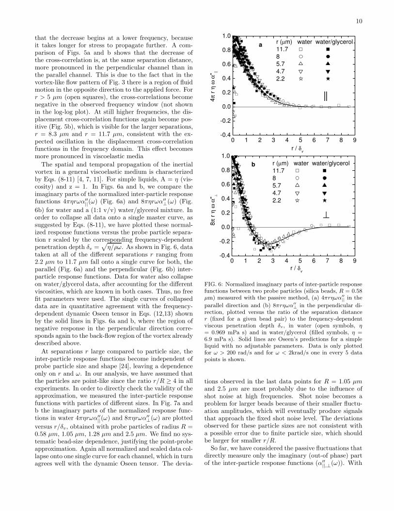
The spatial and temporal propagation of the inertialvortex in a general viscoelastic medium is characterizedby Eqs. (8-11) [4, 7, 11]. For simple liquids, A = η (vis-cosity) and z = 1. In Figs. 6a and b, we compare theimaginary parts of the normalized inter-particle responsefunctions 4πηrωα′′

||(ω) (Fig. 6a) and 8πηrωα′′⊥(ω) (Fig.

6b) for water and a (1:1 v/v) water/glycerol mixture. Inorder to collapse all data onto a single master curve, assuggested by Eqs. (8-11), we have plotted these normal-ized response functions versus the probe particle separa-tion r scaled by the corresponding frequency-dependentpenetration depth δv =

√

η/ρω. As shown in Fig. 6, datataken at all of the different separations r ranging from2.2 µm to 11.7 µm fall onto a single curve for both, theparallel (Fig. 6a) and the perpendicular (Fig. 6b) inter-particle response functions. Data for water also collapseon water/glycerol data, after accounting for the differentviscosities, which are known in both cases. Thus, no freefit parameters were used. The single curves of collapseddata are in quantitative agreement with the frequency-dependent dynamic Oseen tensor in Eqs. (12,13) shownby the solid lines in Figs. 6a and b, where the region ofnegative response in the perpendicular direction corre-sponds again to the back-flow region of the vortex alreadydescribed above.

At separations r large compared to particle size, theinter-particle response functions become independent ofprobe particle size and shape [24], leaving a dependenceonly on r and ω. In our analysis, we have assumed thatthe particles are point-like since the ratio r/R ≥ 4 in allexperiments. In order to directly check the validity of theapproximation, we measured the inter-particle responsefunctions with particles of different sizes. In Fig. 7a andb the imaginary parts of the normalized response func-tions in water 4πηrωα′′

||(ω) and 8πηrωα′′⊥(ω) are plotted

versus r/δv, obtained with probe particles of radius R =0.58 µm, 1.05 µm, 1.28 µm and 2.5 µm. We find no sys-tematic bead-size dependence, justifying the point-probeapproximation. Again all normalized and scaled data col-lapse onto one single curve for each channel, which in turnagrees well with the dynamic Oseen tensor. The devia-

0 1 2 3 4 5 6 7 8 9-0.4

-0.2

0.0

0.2

0.4

0.6

0.8

1.0

||

a

4π r

η ω

α" ||

r / δv

r (µm) water water/glycerol

11.7

8

5.7

4.7

2.2

0 1 2 3 4 5 6 7 8 9-0.4

-0.2

0.0

0.2

0.4

0.6

0.8

1.0

⊥

b r (µm) water water/glycerol

11.7

8

5.7

4.7

2.2

8π r

η ω

α" ⊥

r / δv

FIG. 6: Normalized imaginary parts of inter-particle responsefunctions between two probe particles (silica beads, R = 0.58µm) measured with the passive method, (a) 4πrηωα′′

|| in the

parallel direction and (b) 8πrηωα′′⊥ in the perpendicular di-

rection, plotted versus the ratio of the separation distancer (fixed for a given bead pair) to the frequency-dependentviscous penetration depth δv, in water (open symbols, η= 0.969 mPa s) and in water/glycerol (filled symbols, η =6.9 mPa s). Solid lines are Oseen’s predictions for a simpleliquid with no adjustable parameters. Data is only plottedfor ω > 200 rad/s and for ω < 2krad/s one in every 5 datapoints is shown.

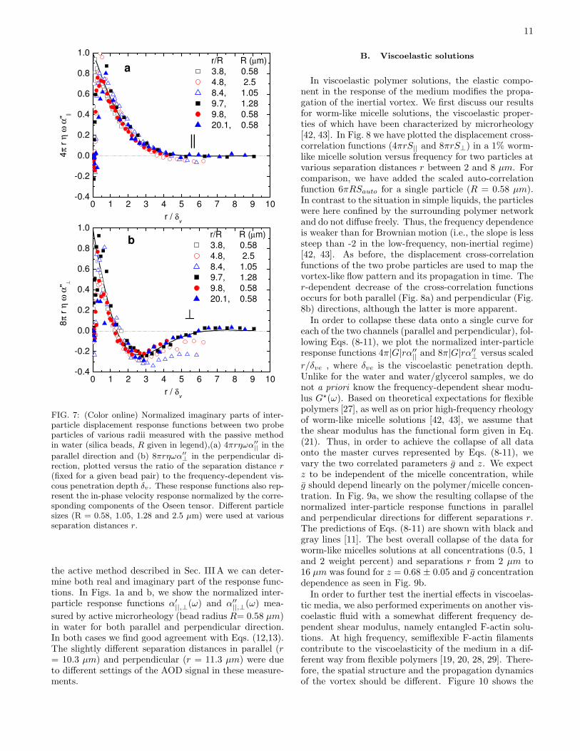
tions observed in the last data points for R = 1.05 µmand 2.5 µm are most probably due to the influence ofshot noise at high frequencies. Shot noise becomes aproblem for larger beads because of their smaller fluctu-ation amplitudes, which will eventually produce signalsthat approach the fixed shot noise level. The deviationsobserved for these particle sizes are not consistent witha possible error due to finite particle size, which shouldbe larger for smaller r/R.

So far, we have considered the passive fluctuations thatdirectly measure only the imaginary (out-of phase) partof the inter-particle response functions (α′′

||,⊥(ω)). With

11

0 1 2 3 4 5 6 7 8 9 10-0.4

-0.2

0.0

0.2

0.4

0.6

0.8

1.0

||

a 4

π r

η ω

α" ||

r / δv

r/R R (µm)

3.8, 0.58

4.8, 2.5

8.4, 1.05

9.7, 1.28

9.8, 0.58

20.1, 0.58

0 1 2 3 4 5 6 7 8 9 10-0.4

-0.2

0.0

0.2

0.4

0.6

0.8

1.0

⊥

b

8π r

η ω

α" ⊥

r / δv

r/R R (µm)

3.8, 0.58

4.8, 2.5

8.4, 1.05

9.7, 1.28

9.8, 0.58

20.1, 0.58

FIG. 7: (Color online) Normalized imaginary parts of inter-particle displacement response functions between two probeparticles of various radii measured with the passive methodin water (silica beads, R given in legend),(a) 4πrηωα′′

|| in the

parallel direction and (b) 8πrηωα′′⊥ in the perpendicular di-

rection, plotted versus the ratio of the separation distance r(fixed for a given bead pair) to the frequency-dependent vis-cous penetration depth δv. These response functions also rep-resent the in-phase velocity response normalized by the corre-sponding components of the Oseen tensor. Different particlesizes (R = 0.58, 1.05, 1.28 and 2.5 µm) were used at variousseparation distances r.

the active method described in Sec. III A we can deter-mine both real and imaginary part of the response func-tions. In Figs. 1a and b, we show the normalized inter-particle response functions α′

||,⊥(ω) and α′′||,⊥(ω) mea-

sured by active microrheology (bead radius R= 0.58 µm)in water for both parallel and perpendicular direction.In both cases we find good agreement with Eqs. (12,13).The slightly different separation distances in parallel (r= 10.3 µm) and perpendicular (r = 11.3 µm) were dueto different settings of the AOD signal in these measure-ments.

B. Viscoelastic solutions

In viscoelastic polymer solutions, the elastic compo-nent in the response of the medium modifies the propa-gation of the inertial vortex. We first discuss our resultsfor worm-like micelle solutions, the viscoelastic proper-ties of which have been characterized by microrheology[42, 43]. In Fig. 8 we have plotted the displacement cross-correlation functions (4πrS|| and 8πrS⊥) in a 1% worm-like micelle solution versus frequency for two particles atvarious separation distances r between 2 and 8 µm. Forcomparison, we have added the scaled auto-correlationfunction 6πRSauto for a single particle (R = 0.58 µm).In contrast to the situation in simple liquids, the particleswere here confined by the surrounding polymer networkand do not diffuse freely. Thus, the frequency dependenceis weaker than for Brownian motion (i.e., the slope is lesssteep than -2 in the low-frequency, non-inertial regime)[42, 43]. As before, the displacement cross-correlationfunctions of the two probe particles are used to map thevortex-like flow pattern and its propagation in time. Ther-dependent decrease of the cross-correlation functionsoccurs for both parallel (Fig. 8a) and perpendicular (Fig.8b) directions, although the latter is more apparent.

In order to collapse these data onto a single curve foreach of the two channels (parallel and perpendicular), fol-lowing Eqs. (8-11), we plot the normalized inter-particleresponse functions 4π|G|rα′′

|| and 8π|G|rα′′⊥ versus scaled

r/δve , where δve is the viscoelastic penetration depth.Unlike for the water and water/glycerol samples, we donot a priori know the frequency-dependent shear modu-lus G⋆(ω). Based on theoretical expectations for flexiblepolymers [27], as well as on prior high-frequency rheologyof worm-like micelle solutions [42, 43], we assume thatthe shear modulus has the functional form given in Eq.(21). Thus, in order to achieve the collapse of all dataonto the master curves represented by Eqs. (8-11), wevary the two correlated parameters g and z. We expectz to be independent of the micelle concentration, whileg should depend linearly on the polymer/micelle concen-tration. In Fig. 9a, we show the resulting collapse of thenormalized inter-particle response functions in paralleland perpendicular directions for different separations r.The predictions of Eqs. (8-11) are shown with black andgray lines [11]. The best overall collapse of the data forworm-like micelles solutions at all concentrations (0.5, 1and 2 weight percent) and separations r from 2 µm to16 µm was found for z = 0.68 ± 0.05 and g concentrationdependence as seen in Fig. 9b.

In order to further test the inertial effects in viscoelas-tic media, we also performed experiments on another vis-coelastic fluid with a somewhat different frequency de-pendent shear modulus, namely entangled F-actin solu-tions. At high frequency, semiflexible F-actin filamentscontribute to the viscoelasticity of the medium in a dif-ferent way from flexible polymers [19, 20, 28, 29]. There-fore, the spatial structure and the propagation dynamicsof the vortex should be different. Figure 10 shows the

12

101

102

103

104

105

10-31

1x10-29

10-27

10-25

1x10-23

1x10-21

a ||

||

4π r

S

[m

3/H

z]

Frequency [Hz]

single particle

r =2µm

r =3µm

r =5µm

r =8µm

101

102

103

104

105

10-31

1x10-29

10-27

10-25

1x10-23

1x10-21

b

⊥

⊥8

π r

S

[m

3/H

z]

Frequency [Hz]

single particle

r =2µm

r =3µm

r =5µm

r =8µm

FIG. 8: Normalized displacement cross-correlation functions4πrS|| (a) and 8πrS⊥ (b) of two probe particles (silica beads,R = 0.58 µm) in worm-like micelle solutions (cm = 1 wt%)versus frequency (f = ω/2π) compared for different separa-tion distances r. The solid lines represent the auto-correlationfunction of a single particle normalized by 6πR. The dashedlines indicate slopes of -2, corresponding to diffusive motion.

collapse of the inter-particle response functions 4π|G|rα′′||

and 8π|G|rα′′⊥ plotted versus scaled distance r/δve onto

two master curves for the parallel and the perpendiculardirection. The actin concentration was 1mg/ml and theprobe radius 0.58 µm and we used separation distancesr ranging from 4.2 µm to 16.2 µm. In an F-actin so-lution of this concentration, the magnitude of the shearmodulus is large, therefore the vortex propagates faster,making it harder to observe. In particular, it was diffi-cult to determine the parameters g and z in this case.We found the best collapse with z = 0.78 ± 0.1 for datataken in passive method. We then fixed z to 0.75 knownfrom the power law dependence behavior reported previ-ously [19, 20, 28, 29], and found g = 0.18 ± 0.13Pa sz.To reduce the large error bars in the passive method, itwould be necessary to repeat our measurements at higher

0 1 2 3 4 5 6-0.4

-0.2

0.0

0.2

0.4

0.6

0.8

1.0

a r (µm) || ⊥

2.3

4.3

6

7.3

10

4π r

|G

| α

" || ;

8π r

|G

| α

" ⊥

r / δve

0.0 0.5 1.0 1.5 2.00.00

0.01

0.02

0.03

0.04

0.05

0.06

0.07

b

g [

Pa

.sz]

Cm (wt%)

FIG. 9: (Color online) (a) Collapse of the imaginary parts ofthe normalized inter-particle response functions (4πr|G|α′′

||(ω)

and 8πr|G|α′′⊥(ω)) between two probe particles (silica beads,

R = 0.58 µm), measured with the passive method for differ-ent separation distances r in worm-like micelle solutions of1 wt%, plotted versus the ratio of the separation distance r(fixed for a given bead pair) to the frequency-dependent vis-coelastic penetration depth δve. Here, the viscoelastic pene-tration depths were determined by varying the parameters gand z in Eqs. (8-11,21) to obtain collapse. Optimal param-eters were z = 0.68 ± 0.05 and g = 0.0275 ± 0.008 Pa sz,where the solvent (water) viscosity has been taken into ac-count. (b) Dependence of (optimal) parameter g on micelleconcentration for a fixed z.

frequencies and/or larger separation distances. Neverthe-less, our results are consistent with prior measurementsand predictions of both parameters.

Independently, we have measured both real, α′||,⊥(ω),

and imaginary, α′′||,⊥(ω), parts of the response functions

directly by actively manipulating one particle and mea-suring the response of the other. In Figs. 2a and b, theparallel (Fig. 2a) and perpendicular (Fig. 2b) complexinter-particle response functions for c = 1 mg/ml F-actinsolutions are shown, probed with beads of 1.28 µm ra-

13

0 1 2 3 4 5

-0.4

-0.2

0.0

0.2

0.4

0.6

0.8

1.0

1.2

4π r

|G

| α

" || ;

8π r

|G

| α

" ⊥

r / δve

r (µm) || ⊥

4.2

5.7

6.9

13

16.2

FIG. 10: (Color online) Collapse of the imaginary parts ofthe normalized inter-particle response functions between twoprobe particles (silica beads, R = 0.58 µm), measured withthe passive method for different separation distances r in F-actin solutions of concentration 1 mg/ml, plotted versus theratio of the separation distance r (fixed for a given bead pair)to the frequency-dependent viscoelastic penetration depthδve. Here, the parameters g and z in Eq. (21) were variedto obtain simultaneous collapse of all data sets onto Eqs. (8-11), using a single set of parameters z and g, while accountingfor the solvent (water) viscosity. We find z = 0.78 ± 0.1, andg = 0.18 ± 0.13 as optimal parameters. Data are presentedfor parallel (closed symbols) and perpendicular (open sym-bols) directions. The solid black line represents Eq. (28) andthe gray line represents Eq. (30), both with z = 0.75 and g =0.2 Pa sz.

dius. Here the inter-particle response functions were fit-ted with Eqs. (8-11) to find parameters g = 0.22±0.05Pa sz and z= 0.78±0.01 simultaneously. Data for bothparallel (r = 12.1 µm) and perpendicular (r = 13.5 µm)channels are compared with z = 0.75 and g = 0.22 Pa sz

in Fig. 2a and b.

The values of z and g found from both methods areconsistent and also agree with results from prior experi-mental microrhelogy and macrorheology experiments forboth entangled actin solutions [18, 19, 20, 28, 29] andworm-like-micelle solutions [42, 43]. To obtain thesevalues it was essential to model the inertial effects in-cluding both polymer and solvent contributions to theshear modulus. We observed that, although the high-frequency rheology of the polymer solution is dominatedby the polymer, the background solvent contributes non-negligibly to the inertial vortex propagation. To test this,we excluded the solvent shear modulus (−iωη) in Eqs. (8-11,21), and analyzed our data assuming a high-frequencyshear modulus of the form G = gωz. For both worm-like micelle solutions and entangled F-actin solutions, wefound much larger values of z ∼ 0.9 and a nonlinear con-centration dependence of g, contrary to expectations.

VI. DISCUSSION

In our experiments we have directly resolved the iner-tial response/flow of fluids on micrometer and microsec-ond time scales using optical trapping and interferometricparticle-tracking. Our results demonstrate that vortic-ity and stress propagate diffusively in simple liquids andsuper-diffusively in viscoelastic media. One consequenceof inertial vortex formation is the long-time tail effect ob-served in light scattering experiments [6]. To connect tothese results, we calculated the velocity auto-correlationof a single particle from the displacement fluctuations.Unfortunately, the effect we are looking for is subtle andis difficult to detect in the presence of other factors. Atthe highest frequencies the vortex is still influenced bythe finite probe size, and at intermediate frequencies theparticle motion is already affected by the laser trap po-tential. The results were thus inconclusive. Similar prob-lems have been reported in Ref. [9]. The effects of in-ertia we have described here set a fundamental limit tothe applicability of two-particle microrheology techniqueswhich are based on the measurement of cross-correlatedposition fluctuations of particles [14, 18, 19, 24, 42]. Iner-tia limits the range of stress propagation at high frequen-cies, stronger in soft media such as those studied herethan in media with higher viscoelastic moduli. Inertiaaffects measurements at frequencies as low as 1 kHz forseparations of order 10 micrometers, showing an appar-ent increase of the measured shear moduli below theiractual values [43]. Since the stress propagation is dif-fusive, or nearly so, even measurements at video ratescan be affected for probe particle separations of order50 micrometers. As we have shown here, these inertialeffects are more pronounced in the perpendicular inter-particle response functions than in the parallel ones. Thissuggests that one should obtain shear moduli from theparallel inter-particle response functions if one doesn’twant to correct for inertia. In a more precise analysisof two-particle microrheology experiments, the fluid re-sponse function can not simply be modeled by a general-ized Stokes-Einstein relationship and has to be correctedfor inertial effects according to the probed frequency aswell as the particles separation. Such corrections, how-ever, will necessarily be limited, given the exponentialattenuation of stress due to inertia.

VII. ACKNOWLEDGMENTS

Actin was purified by K.C. Vermeulen and silica par-ticles were kindly donated by C. van Kats (Utrecht Uni-versity). F. Gittes, J. Kwiecinska, and J. van Mamerenhelped with developing the data analysis software. Wethank D. Frenkel, W. van Saarloos, A.J. Levine andK.M. Addas for helpful discussions. This work was sup-ported by the Foundation for Fundamental Research onMatter (FOM). Further support (C.F.S.) came from theDFG Center for the Molecular Physiology of the Brain

14

(CMPB) and the DFG Sonderforschungsbereich 755.

[1] L.D. Landau and E.M. Lifshitz, Fluid Mechanics,Butterworth-Heinemann (Oxford, 2000).

[2] J. Happel and H. Brenner, Low Reynolds Number Hydro-

dynamics, McGraw-Hill (New York, 1963)[3] E. Guyon et al, Physical Hydrodynamics, Oxford Univer-

sity Press (New York, 2001)[4] C.W. Oseen, Hydrodynamik (Akademische Verlagsge-

sellschaft, Leipzig, 1927), p. 47.[5] B.J. Alder and T.E. Wainwright, Phys. Rev. A 1, 18

(1970).[6] J.P. Boon and A. Bouiller, Phys. Lett. 55A, 391 (1967);

G.L. Paul and P.N. Pusey, J. Phys. A 14, 3301 (1981);K. Ohbayashi, T. Kohno, and H. Utiyama, Phys. Rev. A27, 2632 (1983); D.A. Weitz, D.J. Pine, P.N. Pusey, andR.J.A. Tough, Phys. Rev. Lett. 63, 1747 (1989).

[7] M. Atakhorrami, G.H. Koenderink, C.F. Schmidt, andF.C. MacKintosh, Phys. Rev. Lett. 95, 208302 (2005).

[8] R. Zwanzig and M. Bixon, Phys. Rev. A 2, 2005 (1970);M.H. Ernst, E.H. Hauge, and J.M.J. van Leeuwen, Phys.Rev. Lett. 25, 1254 (1970); J.R. Dorfman and E.G.D.Cohen, Phys. Rev. Lett. 25, 1257 (1970); D. Bedeauxand P. Mazur, Phys. Lett. 43A, 401 (1973); D. Bedeauxand P. Mazur, Physica (Amsterdam) 73, 431 (1974).

[9] B. Lukic, S. Jeney, C. Tischer, et al., Phys. Rev. Lett.95, 160601 (2005).

[10] C. Morkel, C. Gronemeyer, W. Glaser, J. Bosse, Phys.Rev. Lett. 58, 1873 (1987).

[11] T.B. Liverpool and F.C. MacKintosh, Phys. Rev. Lett.95, 208303 (2005).

[12] F. Gittes and C.F. Schmidt, Optics Lett. 23, 7 (1998).[13] M. Atakhorrami, K.M. Addas and C.F. Schmidt, unpub-

lished.[14] J.C. Crocker, M.T. Valentine, E.R. Weeks, T. Gisler,

P.D. Kaplan, A.G. Yodh, and D.A. Weitz, Phys. Rev.Lett. 85, 888 (2000).

[15] J-C. Meiners and S.R. Quake, Phys. Rev. Lett. 82, 2211(1999).

[16] S. Henderson, S. Mitchell, and P. Bartlett, Phys. Rev. E64, 061403 (2001)

[17] L. Starrs and P. Bartlett, Journal of Physics-Cond. Mat.15, S251 (2003).

[18] M.L. Gardel, M.T. Valentine, J.C. Crocker, A.R. Bauschand D.A. Weitz, Phys. Rev. Lett. 91, 158302 (2003).

[19] G.H. Koenderink, M. Atakhorrami, F.C. MacKintosh,C.F. Schmidt, Phys. Rev. Lett. 96:138307 (2006).

[20] F. Gittes, B. Schnurr, P.D. Olmsted, F.C. MacKintoshand C.F. Schmidt, Phys. Rev. Lett. 79, 3286 (1997);B. Schnurr, F. Gittes, F.C. MacKintosh, C.F. Schmidt,Macromolecules 30, 7781 (1997).

[21] D. Mizuno, C. Tardin, C.F. Schmidt, F.C. MacKintosh,Science 315:370 (2007).

[22] L.A. Hough and H.D. Ou-Yang, Phys. Rev. E 65, 021906

(2002).[23] R.B. Bird, R.C. Armstrong, O. Hassager, Dynamics of

Polymeric Liquids, Wiley (New york, 1987).[24] A.J. Levine and T.C. Lubensky, Phys. Rev. Lett. 85,

1774 (2000); A.J. Levine and T.C. Lubensky, Phys. Rev.E 63, 041510 (2001).

[25] F. Brochard and P.G. de Gennes, Macromolecules 10,1157 (1977); S.T. Milner, Phys. Rev. E 48, 3674 (1993).

[26] D. Bedeaux and P. Mazur, Physica (Amsterdam) 76, 235(1974); 76, 247 (1974).

[27] M. Doi and S.F. Edwards, The theory of polymer dynam-

ics, Oxford University Press (New York, 1986).[28] D.C. Morse, Macromolecules 31, 7030 (1998); 31, 7044

(1998).[29] F. Gittes and F.C. MacKintosh, Phys. Rev. E 58, R1241

(1998).[30] For the case of polymer solutions, this represents only the

polymer contribution to the shear modulus. For compar-ison with experiment [7] we have also taken into accountthe solvent contribution in G(ω) = g(−iω)z − iωη.

[31] I. Podlubny, Fractional Differential equations, AcademicPress (London, 1999).

[32] A. Erdelyi (ed.), Higher Transcendental Functions, vol.

3, McGraw-Hill (New York, 1953).[33] R.B. Paris, Proc. Roy. Soc. A., 458, 3041 (2002).[34] J.F. Berret, J. Appell, and G. Porte, Langmuir9, 2851

(1993).[35] J.D. Pardee and J.A. Spudich, in Structural and Contrac-

tile Proteins (PartB: The Contractile Apparatus and theCytoskeleton), ed. by D.W. Frederiksen and L.W. Cun-ningham (Academic Press, Inc., San Diego, 1982), Vol.85, p. 164.

[36] M.W. Allersma, F. Gittes, M.J. deCastro, et al., Biophys.J. 74, 1074 (1998).

[37] D. Mizuno, D.A. Head, F.C. MacKintosh and C.F.Schmidt, unpublished.

[38] E.J.G. Peterman, M.A. van Dijk, L.C. Kapitein, et al.,Rev. Scien. Ins. 74: 3246 (2003).

[39] F. Gittes and C.F. Schmidt, in Methods in Cell Biology(Academic Press, 1998), Vol. 55, p. 129.

[40] L.D. Landau and E.M. Lifshitz and L.P. Pitaevskii Sta-

tistical Physics, (Pergamon Press, Oxford, New York,1980).

[41] T.G. Mason and D.A. Weitz, Phys. Rev. Lett. 75: 2770(1995).

[42] M. Buchanan, M. Atakhorrami, J.F. Palierne, F.C.MacKintosh and C.F. Schmidt, Phys. Rev. E 72, 011504(2005); M. Buchanan, M. Atakhorrami, J.F. Palierne,C.F. Schmidt, Macromolecules 38, 8840 (2005).

[43] M. Atakhorrami and C.F. Schmidt, Rheol. Acta, 45, 449(2006).