KranstauberMovement Ecology (2019) 7:22 https://doi.org/10.1186/s40462-019-0167-3

METHODOLOGY ARTICLE Open Access

Modelling animal movement asBrownian bridges with covariatesBart Kranstauber1,2

Abstract

Background: The ability to observe animal movement and possible correlates has increased strongly over the pastdecades. Methods to analyze trajectories have developed in parallel, but many tools fail to make an immediateconnection between a movement model, covariates of the movement, and animal space use.

Methods: Here I develop a novel method based on the Brownian Bridge Movement Model that facilitatesinvestigating and testing covariates of movement. The model makes it possible to flexibly investigate differentcovariates including, for example, periodic movement patterns.

Results: I applied the Brownian Bridge Covariates Model (BBCM) to simulated trajectories demonstrating its ability toreproduce the parameters used for the simulation. I also applied the model to a GPS trajectory of a meerkat, showingits application to empirical data. The value of the model was shown by testing the interaction between maximal dailytemperature and the daily movement pattern.

Conclusion: This model produces accurate parameter estimates for covariates of the movements and location errorin simulated trajectories. Application to the meerkat trajectory also produced plausible parameter estimates. This newmethod opens the possibility to directly test hypotheses about the influence of covariates on animal movement whilelinking these to space-use estimates.

Keywords: Animal tracking, Brownian bridge covariates model, Brownian bridge movement model, Meerkats,Movement ecology, Suricata suricatta, Utilization distributions

BackgroundThrough movement, animals connect the world: ani-mal movements are key to understanding importantbehavioural, ecological and evolutionary processes suchas migration, social interactions, nutrient fluxes, diseasespread, seed dispersal and gene flow [1]. Although thereis a long history of studying movement and space use,going back to the early work of Burt’s [2] study on homeranges and territoriality, recent technological develop-ments have made it possible to conduct studies over awide range of spatial and temporal scales and with resolu-tions previously unimaginable across a variety of species(e.g. [3–5]).

Correspondence: kranstauber@orn.mpg.de1Department of Evolutionary Biology and Environmental Studies, University ofZurich, Winterthurerstrasse 190, CH-8057 Zurich, Switzerland2Kalahari Meerkat Project, Kuruman River Reserve, P.O. Box 64, Van Zylsrus8467, Northern Cape, South Africa

The analysis of animal tracking data is currentlyundergoing an exciting transformation. Classical tools forestimation of space use and utilization distributions (UDs)such as minimum convex polygons or kernel density sur-faces rely on an independent sample of positions of theindividual [6]. These assumptions are clearly not validespecially for modern data collection technologies, wheretrajectories are typically sampled with high frequencies,often producing several locations per hour. As a result,these methods produce inaccurate estimates of territorysizes and borders.With such highly resolved trajectories itfurther becomes important to account for the accuracy ofthe tracking device, although most classical methods arenot able to do so.Newly developed tools are more suitable for highly

resolved trajectories; they take advantage of the positionalcorrelations instead of removing and/or ignoring them [7].These new tools make use of various underlying move-ment models, such as Brownian bridge (e.g. [8–10]) andbiased random bridge [11]. The dynamic Brownian Bridge

© The Author(s). 2019 Open Access This article is distributed under the terms of the Creative Commons Attribution 4.0International License (http://creativecommons.org/licenses/by/4.0/), which permits unrestricted use, distribution, andreproduction in any medium, provided you give appropriate credit to the original author(s) and the source, provide a link to theCreative Commons license, and indicate if changes were made. The Creative Commons Public Domain Dedication waiver(http://creativecommons.org/publicdomain/zero/1.0/) applies to the data made available in this article, unless otherwise stated.

KranstauberMovement Ecology (2019) 7:22 Page 2 of 10

Movement Model is, for example, useful for calculatingthe area used by animals, while accounting for behaviouralchanges in the movement patterns. This method thoughrequires the behavioural changes to be infrequent relativeto the sampling frequency of the trajectory. By analyzingthe track as a continuous-time stochastic process [7, 12],an accurate description of the movement process andhome range can be obtained.However, most current approaches lack a natural con-

nection to analyze the trajectory with respect to covari-ates. One notable exception is the work of Wilson et al.[13] who integrate environmental covariates using a spa-tially discrete model. Other methods have focused moreon analyzing the trajectory as such, without focusingon space use, by directly calculating metrics from thetrack and comparing these to covariates (e.g. wind andmigration speed, [14, 15]). More recently step-selectionfunctions have become popular; here trajectories are sam-pled to regular intervals and each step is compared to aset of alternative steps that are generated using logisticregressions [16, 17]. This method has the advantage thatit easily incorporates many different covariates of move-ment, but it requires regularized trajectories and thereis no natural relationship to space use [18]. Additionally,step-selection functions do not account for measurementerrors, where the actual location of the animal is not thesame as the reported position. In cases where animalsmove large distances combined with the accuracy of mod-ern tracking technology (e.g. GPS) location errors cansometimes be reasonably ignored. However, for slowermoving animals with frequent location recordings, mea-surement error needs to be accounted for to derive usefulinformation from tracking data [19]. Similarly, the inclu-sion of location errors is important for other trackingmethodologies such as geolocation and the Argos systemthat have considerable location errors [20–22].Nearly all animals show some regular or environmen-

tally induced variation in movement patterns. Animalscommonly have a periodic movement activity: usuallystudied are daily (e.g., nocturnal, diurnal, or crepuscu-lar activity) and yearly (e.g., altitudinal or long-distancemigrations) patterns (e.g. [23–25]). Less frequently stud-ied are movement patterns that relate to the lunarcycle (e.g. [26, 27]). There have been various waysto account for these periodic variations in movement.Approaches based on the Brownian Bridge MovementModel account for behaviourally heterogeneous trajec-tories but do not relate temporal variation to a spe-cific period [9, 10]. These methods rely on a movingwindow approach, therefore it is difficult to describepatterns when observations are infrequent relative tothe period. Alternatively, continuous time movementmodels can include periodic movement patterns [28].A more general approach is to fit a model with

a smoothing term to investigate movement over the day(e.g. [29]). The advantage of using smoothing terms is thatit gives a formal function that can be used to fit interac-tions with other factors influencing the movement patternover the day.Here I develop a method that calculates space use taking

into account movement properties and covariates. Thismodel generalizes the Brownian Bridge Movement Modeland considers factors influencing both the movement andlocation error. Animal movement models based on Brow-nian bridges have found their merits despite the limitingassumptions as isotropic movement and not being boundto ranges. The nature of the covariates influencing move-ment and location error can be flexible, including theinfluence of important ecological and social factors. Thismodel, termed the Brownian Bridge Covariates Model(BBCM), is able to account for errors in the observa-tion process and fit covariates of these errors, ultimatelyleading to a more accurate and predictive model. First, Ievaluate the model by estimating known parameters fromsimulated trajectories. Second, I apply this model to atrajectory of a meerkat (Suricata suricatta), to investi-gate changes to the circadianmovement pattern under theinfluence of weather conditions.

MethodsThis section is divided into three parts: description of themethod, validation of the model by applying it to simu-lated tracks, and use of this method on real tracking dataof a meerkat. All these analyses were conducted in R [30].

Brownian bridges including covariatesPozdnyakov et al. [31] identified that the distancesbetween observations have the following covariancematrix:

�X =

⎡⎢⎢⎢⎢⎢⎣

σ 2τ1 + 2δ2 −δ2 0 · · · 0−δ2 σ 2τ2 + 2δ2 −δ2 · · · 00 −δ2 σ 2τ3 + 2δ2 · · · 0...

......

. . ....

0 0 0 · · · σ 2τn + 2δ2

⎤⎥⎥⎥⎥⎥⎦

Where n is the number of intervals in a trajectory consist-ing of n + 1 locations, τi = ti+1 − ti is the time intervalbetween locations, σ 2 the Brownian motion movementvariance and δ2 the measurement error variance. Buildingon these methods, it is possible to fit covariates to boththe movement trajectory and measurement errors. First,the covariance matrix needs to be adjusted as follows, themeasurement error for each location and motion vari-ance for each segment need to be separated. In that case�X can be formed based on σ 2 = (

σ 21 , . . . , σ 2

n)and

KranstauberMovement Ecology (2019) 7:22 Page 3 of 10

δ2 = (δ21, . . . , δ2n+1

). This creates the following covariance

matrix.

�X =

⎡⎢⎢⎢⎢⎢⎣

σ 21 τ1+δ21+δ22 −δ22 0 · · · 0

−δ22 σ 22 τ2+δ22+δ23 −δ23 · · · 0

0 −δ23 σ 23 τ3+δ23+δ24 · · · 0

......

.... . .

...0 0 0 · · · σ 2

nτn+δ2n+δ2n+1

⎤⎥⎥⎥⎥⎥⎦

To generate σ 2 and δ2 I can rely on frequently used mod-elling tools where a design matrix is multiplied by a vectorof coefficients. For this reason it is important to modelthe movement and location-error variances since they arecumulative in contrast to standard deviations. This meansσ 2 withm covariates can be generated as follows.

⎡⎢⎢⎢⎢⎢⎣

σ 21

σ 22

σ 23...

σ 2n

⎤⎥⎥⎥⎥⎥⎦

=

⎡⎢⎢⎢⎢⎢⎣

x1,1 x1,2 . . . x1,mx2,1 x2,2 . . . x2,mx3,1 x3,2 . . . x3,m...

.... . .

...xn,1 xn,2 . . . xn,m

⎤⎥⎥⎥⎥⎥⎦

⎡⎢⎢⎢⎣

βσ 2,1βσ 2,2...

βσ 2,m

⎤⎥⎥⎥⎦

Similarly, δ2 can be generated based on the location-error covariates. Using this strategy and the likelihoodequation given by Pozdnyakov et al. [31], now the likeli-hood can be evaluated based onβσ 2 andβδ2 . Here I choseto evaluate this equation usingMarkov chainMonte Carlo(MCMC) methods. To do this I relied on the stan libraryaccessed through the rstan R package [32]; for computa-tional efficiency all covariates were scaled. Through thislibrary, direct optimization of the parameters is also possi-ble. For all model fits I evaluated the trace plots to confirmthat all chains are well mixed and the warmup period issufficiently long. I report maximal R̂ values to asses modelfit [33]; values above 1.1 indicate a poor model fit.

Estimate origin of the trajectoryThe original estimation of σ and δ described by Pozd-nyakov et al. [31] makes the assumption that the originof the trajectory is located at 0, 0 and thus known. Sinceparameter estimation depends on the distances betweenlocations, this has no consequences for the parameter esti-mation. In most tracking studies this assumption, that thestarting location is known, is difficult to justify. Often therelease location of the animal is recorded with similaraccuracy as the other locations in the track. Furthermore,the first recording by an animal-borne tracking device isgenerally not recorded at the same time as the release.Therefore I expanded earlier analysis by including the esti-mation of the first location; knowing the start of the trajec-tory is important for calculating the location of the UD inspace. Estimation of the first location can be achieved byextending the likelihood function to include the likelihoodof this location. The distance between the first location

and the first observed location has a variance of δ21, whileit has covariance with the first step length of −δ21. Thisprocedure creates the following covariance matrix thatstill profits from the tribanded nature for efficient modelevaluation.

�X =

⎡⎢⎢⎢⎣

δ21 −δ21 0 · · ·−δ21 σ 2

1 τ1 + δ21 + δ22 −δ22 · · ·0 −δ22 σ 2

2 τ2 + δ22 + δ23 · · ·...

......

. . .

⎤⎥⎥⎥⎦

To estimate the likelihood of the combined initial loca-tion and increments of the trajectory, the vector con-taining the expected values also needs to be updated.Previously this vector consisted purely of expected dis-tances between locations, which are zero. To include thefirst location the deviations from expected can be repre-sented as follows X = (Z0 − γ ,X1, . . . ,Xn)ᵀ, where γ isthe origin of the trajectory.

Generating covariatesFor calculating the design matrix, I utilized readily avail-able R tools, making it possible to profit from the familiarformula specification. For the movement variance, it isimportant to realize that these coefficients are represen-tative for the complete interval between two locations;covariates thus need to represent the conditions duringthis period and not conditions at the start or end location.Special care needs to be taken since variances are mod-

elled; this means all estimates need to be positive. Toenforce this, either models with an intercept can be usedor models where all values for the first covariate are eithercompletely positive or negative. In both cases the minimalor maximal value for the first parameter depends on theother parameter estimates and can be calculated duringsampling. These constraints on the covariates ensure thesampled parameters result in positive variance estimates.

Periodicmovement covariatesAn important covariate of movement I included in themodel is the periodic movement pattern. This was doneby estimating circular smoothing functions as a covariateof the movement variance. Smooths are flexible tools fordescribing these patterns withoutmaking a priori assump-tions. By using circular smoothers there is no need toartificially cut the day or other time periods over whichthe movement is estimated at a specific time point. Iused cubic B splines, which consist of four segments persmoothing term. These splines give us the instantaneousmovement rate at any time. Since the σ 2

m values are repre-sentative of the movement rate over the whole segment, Ineeded to derive the average movement rate for each seg-ment. This can be accomplished by integrating the splinesover the time period between observations and then divid-ing it by the time interval. For regular splines this can be

KranstauberMovement Ecology (2019) 7:22 Page 4 of 10

achieved using analytical integration, allowing for quickcalculations. The disadvantage of this approach is that theintercept is included in the smoothing term. When sucha model is combined with an intercept it will have mul-tiple solutions. I used an alternative approach, where Iseparated out the constants in a model. No attempt hasbeenmade to solve this analytically; I relied on the numer-ical integration of existing implementations [34]. Thesealso give us additional flexibility with the specification ofsmoothing terms, as it opens the possibility of customknot placement. Non-regular knot placement is mainly ofuse when the tracked individual has not been observedfor a longer time period when the tags are turned off ornot observed during the resting period. Within this timeperiod there are no observations and thus there is noinformation on the movement pattern. When a uniformdistribution of the smoothing terms would have beenused, information to estimate the smoothing terms duringthe period when the GPS was turned off is lacking.

ValidationTo validate the model I first simulated irregular tra-jectories with various parameters to investigate if themodel can accurately estimate parameters without peri-odic terms. To investigate the accuracy of these estima-tions I varied the length of the trajectories (n = 100,200, 500, 1000, 2000, 5000 and 10000). For each trajec-tory length three replicates were calculated. The trackswere simulated including a continuous covariate of boththe movement variance and the location error and a dis-crete covariate with three different levels of both. Foreach segment, one of three movement states was sampled(Pr =[ 0.5, 0.2, 0.3] ), each state had its own movementrate (σ 2 =[ 0.3, 0.8, 2] ), the continuous movement covari-ate was sampled uniformly random between 0.0 and 0.5and had a slope of 2. For the location error, three cate-gories were sampled (Pr =[ 0.25, 0.5, 0.25] ) per location,each category was associated with a specific locationerror (δ2 =[ 3, 3.9, 6] ), the continuous error covariate wassampled between -1.0 and 1.0 and had a slope of 0.4.Time intervals were generated by adding one to a gammadistribution (α = 3, β = 0.1, mean time lag = 31.06s). For these trajectories, 10 parameters were estimatedin total: four relating to the location error, four relatingto the movement, and two for the start location. Themodel was fitted based on intercepts and treatment con-trast with fourMCMC chains, each with 5000 iterations ofwhich 2500 were warmup iterations; chains were thinnedby retaining every tenth iteration. To assess the impor-tance of incorporating location error I have also fittedthese models using only a single intercept to describe thesame trajectories.To investigate the ability of the model to describe peri-

odic patterns I simulated trajectories of a 10-day duration.

These trajectories were simulated with five different cir-cadian movement patterns, consisting of either six or tenknots. Models were estimated with the same number ofknots as specified for the simulated trajectory. Trajecto-ries included a location error of δ2 = 10. To investigate theaccuracy of these estimations as a function of sample size Irepeated the analysis four times with track lengths varyingbetween 500 and 5000 locations. For optimization I used5000 MCMC iterations replicated across four chains. Forthese validations I assess the ability to reproduce knownsimulation parameters.

Application to tracking dataI tested the method described above by applying it to atrajectory of a meerkat, which has been followed over 29days. Meerkats live in social groups ranging from 2 to 50individuals, where the dominant pair controls most breed-ing. At the Kalahari Meerkat Project detailed behaviouralobservations have been conducted for over 20 years (foran overview see [35]). Meerkat groups emerge from theirburrows around sunrise and collectively forage predom-inantly for invertebrate prey while moving. During sum-mer the groups stop moving during the hottest part of theday when they take a break and often rest in the shade.In the afternoon meerkats resume foraging before groupsreturn to a sleeping burrow [36]. The meerkat was fit-ted with a collar on 25th of January 2018; the collar wasremoved after three months. At the time of capture theindividual weighed 606g. The GPS logger (weight 20 g,Gipsy 5, Technosmart, Rome, Italy) was programmed totake 5 locations with a 1 Hz frequency every 5 minutes for12 hours a day from 7 am until 7 pm. Outliers were fil-tered by a set of criteria based on distances and turn angleseither between locations or bursts, high speeds betweenone or more bursts and a high spread of locations withina burst. The criteria used were validated using indepen-dent observations of the meerkat group. From the original16169 locations, 13513 observations were retained. Withthis dataset, I explored different periodic smoothing todescribe the activity over the day. Since there are no obser-vations during the night time I only specified knots duringthe daytime. The first knot is specified at the first observa-tion across days while the last knot is specified at the lastlocation. The number of knots varied between 5 and 12 toinvestigate the number of knots producing the best-fittingmodel. For location error I did not vary the terms; I fitteda model without intercept, taking the squared HorizontalDilution Of Precision (HDOP) as the only covariate.The capabilities of the model to test a hypothesis were

investigated by estimating the response of the meerkatto maximal daily temperature. Temperature data werederived from the reserve’s weather station and variedbetween 24.1 ◦C and 40.8 ◦C during the tracking period.I tested whether meerkats had a reduced foraging and

KranstauberMovement Ecology (2019) 7:22 Page 5 of 10

thus movement activity on hot days during the late partof the morning when temperatures rise in comparison tothe activity pattern on the other cooler days. As a thresh-old for hot days I used 35 ◦C; this same threshold isused for bird studies in the region [37]. I started usinga model with the same number of knots as the modelfound to best describe themovement. On hot days I dupli-cated the smoothing terms that peak between 9 and 12o’clock. In this way themodel can describe differentmove-ment patterns within the morning time period for hot andcool days.

ResultsValidationThe model successfully reproduced the parameters usedto simulate trajectories (Fig. 1): the R̂ values for all param-eters were below 1.009. Confidence intervals of the esti-mated parameters overlapped with the values used forsimulations independent of the length of the simulatedtrajectory. For these and all other models, parameter esti-mates are shown in the supplementary material. With

increasing trajectory length the confidence interval forthe estimated parameter shrinks considerably. The esti-mated parameters perform equally well for location erroras for movement parameters. The benefits of incorpo-rating additional variables to appropriately describe thelocation error depend on the trajectory length. For trajec-tories longer than 5000 observations the AIC differencefor models incorporating covariates of the location errorwas always positive (range from 4.4 to 31.9), vice versafor trajectories shorter than 200 all AIC differences werenegative (range from -7.8 to -1.4). To assess the influenceof error modelling on the fit of movement parameters Icalculated the variance of the difference between the sim-ulated values and the MCMC chains. The variance washigher for 19 out of 28 parameters in models withouterror modelling.I found that simulated daily movement patterns were

well captured by the model (Fig. 2, R̂ < 1.013). This fit isindependent of the number of changes in the pattern. Evenat the smallest track length of 500 the general featuresof the movement patterns are retained. With increasing

Fig. 1 Results of fitting the BBCM to simulated trajectories. Each simulation was based on 10 parameters that were estimated using the model. Eachpanel displays the estimations for one parameter; the set parameter value is shown by the horizontal line. Simulations were conducted for threereplicates of seven different trajectory lengths. Vertical lines indicate 50% and 95% confidence intervals from the MCMC simulation; points reflectthe maximum likelihood estimate

KranstauberMovement Ecology (2019) 7:22 Page 6 of 10

Fig. 2 Results from fitting daily movement smoothers to test trajectories. I simulated four daily movement patterns; for each pattern four differenttrajectory lengths have been simulated, this length is indicated in the subpanel header. Each daily movement pattern is shown in a different colour.The model fit to the simulated trajectories is visualized by the maximum likelihood estimate as a solid line with the 50% and 95% confidenceintervals shown by the darker and lighter shading, respectively. Dashed lines depict the simulated daily movement patterns

sample size the confidence intervals become more narrowand still include the simulated pattern.

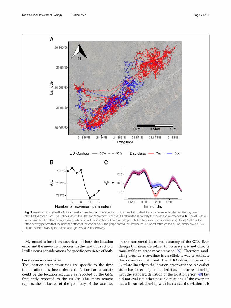
Application to tracking dataI successfully fitted models to the meerkat trajectory(Fig. 3a). The model fit strongly depended on the num-ber of knots; models with the lowest AIC used ten knots(Fig. 3b, for all models R̂ < 1.007). As the smoothers forma circular approximation of the activity, the movementpattern throughout the day can be calculated. During thenight the confidence interval was much wider since thereare no observations at night; the variation in movementduring the night cannot be described. The average esti-mated σ 2

m during the night is 0.85 m2/s which is muchlower than the daily average of 8.19m2/s.On 22 out of 29 days the air temperature rose above

35 ◦C. When comparing the model taking hot days intoaccount, the AIC drops by 35.7 points compared to thereference model; parameters of this model have a R̂ valuebelow 1.007. Visualization of these model outputs showedthat during the cooler days there was more movementin the late morning compared to the warmer days(Fig. 3c).

DiscussionResults of this study suggest that the described BBCMapproach was successful in capturing movement patternsthat included covariates. The model worked accuratelyto describe the relationships between movement and

different covariates, independent of whether these covari-ates were categorical, continuous or a daily movementpattern. A combination of linear and factorial covari-ates, as well as periodic covariates, have been testedhere using simulations. A comparison with models onlyincorporating one estimate for location error shows thatextra parameters accounting for covariates of the locationerror results in an improved model fit for longer trajec-tories. I also used this method successfully to investigatethe trajectory of a meerkat, to test specific hypothe-ses about its movement behaviour. Using the proposedBBCM, the observed movement pattern is used to esti-mate the influence of covariates and periodic movementpatterns; these are subsequently integrated into the cal-culation of the UDs. Models of the movement processand UDs are important for many different subsequentanalytical approaches in the field of movement ecology.The BBCM is computationally efficient because it prof-

its from the tribandedmatrix inversion; it can comfortablybe used to investigate trajectories with (10,000) loca-tions. Computational time also depends on the number ofcovariates and mostly on the method of evaluation, eitherthrough MCMC or optimization. An interesting alterna-tive is to use Kalman filters, which has been explored byFleming et al. [38], making it possible to evaluate mod-els efficiently. This approach would also profit from theability to integrate the persistence of motion. Future workis needed to evaluate this and compare its advantages anddisadvantages.

KranstauberMovement Ecology (2019) 7:22 Page 7 of 10

A

B C

Fig. 3 Results of fitting the BBCM to a meerkat trajectory. a | The trajectory of the meerkat studied; track colour reflects whether the day wasclassified as cool or hot. The isolines reflect the 50% and 95% contour of the UD calculated separately for cooler and warmer days. b | The AIC of thevarious models fitted to the trajectory as a function of the number of knots. AIC drops until ten knots and then increases slightly. c | A plot of thefitted activity pattern that includes the effect of the cooler days. The graph shows the maximum likelihood estimate (black line) and 50% and 95%confidence intervals by the darker and lighter shade, respectively

My model is based on covariates of both the locationerror and the movement process. In the next two sectionsI will discuss considerations for specific covariates of both.

Location-error covariatesThe location-error covariates are specific to the timethe location has been observed. A familiar covariatecould be the location accuracy as reported by the GPS,frequently reported as the HDOP. This measurementreports the influence of the geometry of the satellites

on the horizontal locational accuracy of the GPS. Eventhough this measure relates to accuracy it is not directlytranslatable to error measurement [39]. Therefore mod-elling error as a covariate is an efficient way to estimatethe conversion coefficient. The HDOP does not necessar-ily relate linearly to the location-error variance. An earlierstudy has for example modelled it as a linear relationshipwith the standard deviation of the location error [40] butdid not evaluate other possible relations. If the covariatehas a linear relationship with its standard deviation it is

KranstauberMovement Ecology (2019) 7:22 Page 8 of 10

advisable to transform it by squaring in order to makethe relationship with the location-error variance linear.Different transformations of continuous covariates can beexplored to identify the one that produces a linear relationwith the modelled variances.Frequently the influence of habitat on location error is

discussed. Forests and other covered habitats generallyproduce larger location errors [19, 41, 42]. Including theseis possible if the observed locations are annotated withhabitat information. The difficulty is that the habitat atan observed location is not necessarily the same as thehabitat on the true position of the animal with the GPStag. This means that the habitat where the GPS obtainedthe location with the associated error is not necessarilythe one that is modelled. This is likely not very problem-atic in cases where the habitat is continuous and locationsrarely fall close (i.e. within the location error) to an edgeof a habitat and thus has a low likelihood to be associatedwith an incorrect habitat classification. In cases where thehabitat is a fine mosaic of different habitat types it mightnot be possible to include habitat reliably without furtherresearch.Frequently animals are tracked using a combination of

technologies. A well-known example is GPS-Argos track-ing that produces both location estimates through Argosand GPS. On other occasions animals are tracked using acombination of visual observations and by technologicalmeans. Including tracking technology as a covariate in amodel for location error is a viable approach to accountfor differing location errors produced by different trackingtechnologies.

Movement variance covariatesCovariates of movement require slightly more consider-ation compared to the location-error covariates. Sincethese are representative for the time periods between theobservations they need to be summarized for this time.Besides periodic movement, one likely covariate for themovement rate is the acceleration as measured by mod-ern tags. If acceleration is to be included as a covariateit needs to be averaged over the entire segment betweentwo observations. This could be achieved by includingtime-weighted averaged Overall Dynamic Body Acceler-ation (ODBA) as an index of activity. It has been foundthat ODBA is an accurate predictor of movement speed[43], and thus it could be an important covariate. A sec-ond solution could be to classify acceleration bursts aseither active or non-active and use the proportion ofactive acceleration burst as a covariate (e.g. [11]). Takinginto account this covariate becomes especially importantif sampling is dependent on acceleration as is done withacceleration-informed GPS sampling (i.e. [44]).The BBCM is centred around temporally varying

covariates; these are by no means the only important

factor to understand space use and movement of ani-mals. A large class of covariates that have not beenintegrated here are spatially distributed environmentalvariables (e.g. habitat type and elevation). This class ofcovariates also include barriers to movement that cannot be crossed; these range from fences to shorelines.An important contribution has recently been made byWilson et al. [13] who develop a model to analyse move-ment while incorporating environmental covariates. Theirmodel depends on a discretization of space in contrastto the BBCM that treats space as continuous. The laterhas the advantage that probabilities for any position inspace can be calculated directly. Work in the near futureshould focus on integrating both approaches where differ-ent kinds of covariates can be easily combined, preferablyin continuous space.

ConclusionUsing the BBCM it is possible to directly test hypothe-ses concerning the movement patterns of animals, takinginto account observation errors and other covariates. Myapproach is based on the existing rstan library for modelevaluation, making it possible to profit from existing toolsin the R environment. By using these tools new modelscan be implemented and evaluated efficiently to allow forflexible hypothesis testing.

AbbreviationsBBCM: Brownian bridge covariates model; HDOP: Horizontal dilution ofprecision; MCMC: Markov chain monte carlo; ODBA: Overall dynamic bodyacceleration; UD: Utilization distribution

AcknowledgementsI acknowledge the Kalahari Meerkat Project headed by Marta Manser and TimClutton-Brock and the Kalahari Research Trust these are supported by theMava Foundation, this facilitated the work on the meerkat population. TheKalahari Meerkat Project is facilitated by the Kalahari Research Trust located atthe Kuruman River Reserve and receives logistical support from the MammalResearch Institute of the University of Pretoria. In addition, I thank Jacob Brownfor deploying and retrieving the tags. Furthermore, I profited from valuablediscussion with Stefanie Muff, Chris H. Fleming and Vladimir Pozdnyakov. Ilikewise thank Anne Scharf, Scott LaPoint, Megan Wyman the editor and twoanonymous reviewers for valuable feedback on the manuscript.

Authors’ contributionsBK designed the project, developed the methods, conducted the analysis andwrote the paper. The author read and approved the final manuscript.

FundingThe Promotor Stiftung financed the meerkat tracking work. TheForschungskredit from the University of Zurich (FK-18-110) financed themodel development work.

Availability of data andmaterialsThe model developed here is available in the R package“moveBrownianModel” (https://gitlab.com/bartk/moveBrownianModel).

Ethics approval and consent to participateThis work was permitted by the Northern Cape Department of Environmentand Nature Conservation of South Africa (FAUNA 1020/2016) and theUniversity of Pretoria Animal Ethics Committee (“Movement and groupco-ordination in meerkats (Suricata suricatta)”, EC031-17).

KranstauberMovement Ecology (2019) 7:22 Page 9 of 10

Consent for publicationNot applicable

Competing interestsThe author declares that he/she has no competing interests.

Received: 25 January 2019 Accepted: 4 June 2019

References1. Kays R, Crofoot MC, Jetz W, Wikelski M. Terrestrial animal tracking as an

eye on life and planet. Science. 2015;348(6240):aaa2478–aaa. Availablefrom: http://www.sciencemag.org/content/348/6240/aaa2478.

2. Burt WH. Territoriality and home range concepts as applied to mammals.J Mammal. 1943;24(3):346–52.

3. Strandburg-Peshkin A, Farine DR, Couzin ID, Crofoot MC. Shareddecision-making drives collective movement in wild baboons. Science.2015;348(6241):1358–61. Available from: http://www.sciencemag.org/content/348/6241/1358.

4. Flack A, Fiedler W, Blas J, Pokrovsky I, Kaatz M, Mitropolsky M, et al.Costs of migratory decisions: A comparison across eight white storkpopulations. Sci Adv. 2016;2(1):e1500931. Available from: http://advances.sciencemag.org/content/2/1/e1500931.

5. Tucker MA, Böhning-Gaese K, Fagan WF, Fryxell JM, Moorter BV, AlbertsSC, et al. Moving in the Anthropocene: Global reductions in terrestrialmammalian movements. Science. 2018;359(6374):466–9. Available from:http://science.sciencemag.org/content/359/6374/466.

6. Worton BJ. Kernel Methods for Estimating the Utilization Distribution inHome-Range Studies. Ecology. 1989;70(1):164–8. Available from: http://www.esajournals.org/doi/abs/10.2307/1938423.

7. Fleming CH, Calabrese JM, Mueller T, Olson KA, Leimgruber P, FaganWF, et al. From Fine-Scale Foraging to Home Ranges: A SemivarianceApproach to Identifying Movement Modes across Spatiotemporal Scales.Am Natural. 2014;183(5):E154–67. Available from: http://www.jstor.org/stable/10.1086/675504.

8. Horne JS, Garton EO, Krone SM, Lewis JS. Analyzing animal movementsusing Brownian bridges. Ecology. 2007;88(9):2354–63. Available from:http://www.ncbi.nlm.nih.gov/pubmed/17918412.

9. Kranstauber B, Kays R, LaPoint SD, Wikelski M, Safi K. A dynamicBrownian bridge movement model to estimate utilization distributionsfor heterogeneous animal movement. J Animal Ecol. 2012;81(4):738–46.Available from: http://onlinelibrary.wiley.com/doi/10.1111/j.1365-2656.2012.01955.x/abstract.

10. Kranstauber B, Safi K, Bartumeus F. Bivariate Gaussian bridges: directionalfactorization of diffusion in Brownian bridge models. Mov Ecol. 2014;2(1):5. Available from: http://www.movementecologyjournal.com/content/2/1/5/abstract.

11. Benhamou S. Dynamic Approach to Space and Habitat Use Based onBiased Random Bridges. PLoS ONE. 2011;6(1):e14592. Available from:http://dx.doi.org/10.1371/journal.pone.0014592.

12. Fleming CH, Calabrese JM. A new kernel density estimator for accuratehome-range and species-range area estimation. Methods Ecol Evol.2016;8(5):571–9. Available from: http://onlinelibrary.wiley.com/doi/10.1111/2041-210X.12673/abstract.

13. Wilson K, Hanks E, Johnson D. Estimating animal utilization densitiesusing continuous-time Markov chain models. Methods Ecol Evol.2018;9(5):1232–40. Available from: https://besjournals.onlinelibrary.wiley.com/doi/abs/10.1111/2041-210X.12967.

14. Shamoun-Baranes J, Baharad A, Alpert P, Berthold P, Yom-Tov Y, Dvir Y,et al. The effect of wind, season and latitude on the migration speed ofwhite storks Ciconia ciconia, along the eastern migration route. J AvianBiol. 2003;34(1):97–104.

15. Safi K, Kranstauber B, Weinzierl R, Griffin L, Rees EC, Cabot D, et al. Flyingwith the wind: scale dependency of speed and direction measurementsin modelling wind support in avian flight. Mov Ecol. 2013;1(1):4. Availablefrom: http://www.movementecologyjournal.com/content/1/1/4/abstract.

16. Fortin D, Beyer HL, Boyce MS, Smith DW, Duchesne T, Mao JS. Wolvesinfluence elk movements: behaviour shapes a trophic cascade inYellowstone national park. Ecology. 2005;86(5):1320–30. Available from:http://www.esajournals.org/doi/abs/10.1890/04-0953?journalCode=ecol.

17. Thurfjell H, Ciuti S, Boyce MS. Applications of step-selection functions inecology and conservation. Mov Ecol. 2014;2(1):4. Available from: http://www.movementecologyjournal.com/content/2/1/4/abstract.

18. Signer J, Fieberg J, Avgar T. Estimating utilization distributions fromfitted step-selection functions. Ecosphere. 2017;8:4. Available from: http://onlinelibrary.wiley.com/doi/10.1002/ecs2.1771/abstract.

19. Weerd Nd, Langevelde Fv, Oeveren Hv, Nolet BA, Kölzsch A, Prins HHT,et al. Deriving Animal Behaviour from High-Frequency GPS: TrackingCows in Open and Forested Habitat. PLoS ONE. 2015;10(6):129030.Available from: https://journals.plos.org/plosone/article?id=10.1371/journal.pone.0129030.

20. Keating KA, Brewster WG, Key CH. Satellite Telemetry: Performance ofAnimal-Tracking Systems. J Wildl Manag. 1991;55(1):160–71. Availablefrom: http://www.jstor.org/stable/3809254.

21. Douglas DC, Weinzierl RC, Davidson S, Kays R, Wikelski M, Bohrer G.Moderating Argos location errors in animal tracking data. Methods EcolEvol. 2012;3(6):999–1007. Available from: http://doi.wiley.com/10.1111/j.2041-210X.2012.00245.x.

22. Fudickar AM, Wikelski M, Partecke J. Tracking migratory songbirds:accuracy of light-level loggers (geolocators) in forest habitats. MethodsEcol Evol. 2012;3(1):47–52. Available from: http://onlinelibrary.wiley.com/doi/10.1111/j.2041-210X.2011.00136.x/abstract.

23. Merrill SB, Mech LD. The Usefulness of GPS Telemetry to Study WolfCircadian and Social Activity. Methods Soc Bull (1973-2006). 2003;31(4):947–60. Available from: https://www.jstor.org/stable/3784439.

24. Morellet N, Bonenfant C, Börger L, Ossi F, Cagnacci F, Heurich M, et al.Seasonality, weather and climate affect home range size in roe deeracross a wide latitudinal gradient within Europe. J Animal Ecol. 2013;82(6):1326–39. Available from: https://besjournals.onlinelibrary.wiley.com/doi/abs/10.1111/1365-2656.12105.

25. Dominoni DM, Åkesson S, Klaassen R, Spoelstra K, Bulla M. Methods infield chronobiology Philosophical Transactions of the Royal Society ofLondon Series B. Biol Sci. 2017;372(1734):20160247.

26. Cruz SM, Hooten M, Huyvaert KP, Proaño CB, Anderson DJ, Afanasyev V,et al. At–Sea Behavior Varies with Lunar Phase in a Nocturnal PelagicSeabird, the Swallow-Tailed Gull. PLoS ONE. 2013;8(2):e56889. Availablefrom: https://journals.plos.org/plosone/article?id=10.1371/journal.pone.0056889.

27. Palmer MS, Fieberg J, Swanson A, Kosmala M, Packer C. A ‘dynamic’landscape of fear: prey responses to spatiotemporal variations inpredation risk across the lunar cycle. Ecol Lett. 2017;20(11):1364–73.Available from: http://onlinelibrary.wiley.com/doi/10.1111/ele.12832/abstract.

28. Péron G, Fleming CH, de Paula RC, Calabrese JM. Uncovering periodicpatterns of space use in animal tracking data with periodograms,including a new algorithm for the Lomb-Scargle periodogram andimproved randomization tests. Mov Ecol. 2016;4(1):19. Available from:https://doi.org/10.1186/s40462-016-0084-7.

29. Martin J, Moorter Bv, Revilla E, Blanchard P, Dray S, Quenette PY, et al.Reciprocal modulation of internal and external factors determinesindividual movements. J Anim Ecol. 2013;82(2):290–300. Available from:https://besjournals.onlinelibrary.wiley.com/doi/abs/10.1111/j.1365-2656.2012.02038.x.

30. R Core Team. R: A Language and Environment for Statistical Computing.Version 3.5.1. Vienna; 2018. Available from: https://www.R-project.org/.

31. Pozdnyakov V, Meyer TH, Wang YB, Yan J. On Modeling AnimalMovements Using Brownian Motion with Measurement Error. Ecology.2014;95(2):247–53. Available from: http://www.esajournals.org/doi/abs/10.1890/13-0532.1.

32. Guo J, Gabry J, Goodrich B. rstan: R Interface to Stan R package version2.18.2. 2018. Available from: https://CRAN.R-project.org/package=rstan.

33. Gelman A, Rubin DB. Inference from iterative simulation using multiplesequences. Stat Sci. 1992;7(4):457–72.

34. Wood S. mgcv: Mixed GAM Computation Vehicle with AutomaticSmoothness Estimation. R package version 1.8-26. 2018. Available from:https://CRAN.R-project.org/package=mgcv.

35. Clutton-Brock TH, Manser MB. Meerkats: Cooperative breeding in theKalahari. In: Cooperative Breeding in Vertebrates. Cambridge UniversityPress; 2016. p. 294. Available from: http://books.google.com/books?hl=en&amp;lr=&amp;id=P70wCwAAQBAJ&amp;oi=fnd&amp;pg=PA294&amp;dq=info:V6E38O9mS6gJ:scholar.google.com&amp;ots=dZjq9dUFvh&amp;sig=rPqFZ2zt0N20rt2yFW7pBbi5klk.

KranstauberMovement Ecology (2019) 7:22 Page 10 of 10

36. Gall GEC, Strandburg-Peshkin A, Clutton-Brock T, Manser MB. As duskfalls: collective decisions about the return to sleeping sites in meerkats.Anim Behav. 2017;132:91–9. Available from: http://www.sciencedirect.com/science/article/pii/S0003347217302506.

37. Cunningham SJ, Martin RO, Hojem CL, Hockey PAR. Temperatures inExcess of Critical Thresholds Threaten Nestling Growth and Survival in ARapidly-Warming Arid Savanna: A Study of Common Fiscals. PLoS ONE.2013;8(9):e74613. Available from: https://journals.plos.org/plosone/article?id=10.1371/journal.pone.0074613.

38. Fleming CH, Sheldon D, Gurarie E, Fagan WF, LaPoint S, Calabrese JM.Kálmán filters for continuous-time movement models. Ecol Informa.2017;40:8–21. Available from: http://www.sciencedirect.com/science/article/pii/S1574954117301115.

39. Recio MR, Mathieu R, Denys P, Sirguey P, Seddon PJ. LightweightGPS-Tags, One Giant Leap for Wildlife Tracking?An Assessment Approach.PLoS ONE. 2011;6(12):e28225. Available from: http://journals.plos.org/plosone/article?id=10.1371/journal.pone.0028225.

40. Adams AL, Dickinson KJM, Robertson BC, Heezik Yv. An Evaluation of theAccuracy and Performance of Lightweight GPS Collars in a SuburbanEnvironment. PLoS ONE. 2013;8(7):e68496. Available from: https://journals.plos.org/plosone/article?id=10.1371/journal.pone.0068496.

41. Rempel RS, Rodgers AR, Abraham KF. Performance of a GPS AnimalLocation System under Boreal Forest Canopy. J Wildl Manag. 1995;59(3):543–51. Available from: https://www.jstor.org/stable/3802461.

42. DeCesare NJ, Squires JR, Kolbe JA. Effect of forest canopy on GPS-basedmovement data. Wildl Soc Bull. 2005;33(3):935–41. Available from: https://wildlife.onlinelibrary.wiley.com/doi/abs/10.2193/0091-7648%282005%2933%5B935%3AEOFCOG%5D2.0.CO%3B2.

43. Bidder OR, Soresina M, Shepard ELC, Halsey LG, Quintana F,Gómez-Laich A, et al. The need for speed: testing acceleration forestimating animal travel rates in terrestrial dead-reckoning systems.Zoology. 2012;115(1):58–64. Available from: http://www.sciencedirect.com/science/article/pii/S0944200611000985.

44. Brown DD, LaPoint S, Kays R, Heidrich W, Kümmeth F, Wikelski M.Accelerometer-informed GPS telemetry: Reducing the trade-off betweenresolution and longevity. Wildl Soc Bull. 2012;36(1):139–46. Availablefrom: http://onlinelibrary.wiley.com/doi/10.1002/wsb.111/full.

Publisher’s NoteSpringer Nature remains neutral with regard to jurisdictional claims inpublished maps and institutional affiliations.