Estimating ground motions using recorded accelerograms

E S T I M A T I N G G R O U N D M O T I O N S

U S I N G R E C O R D E D A C C E L E R O G R A M S

THOMAS H. HEATON*, FUMIKO TAJIMA**

Dames and Moore, 445 S. Figueroa St., Los Angeles, Calif., U.S.A.

and

ANN WILDENSTEIN MORI***

Exxon Production Research Co., P.O. Box 2189, Houston, Tex., U.S.A.

Abstract. A procedure for estimating ground motions using recorded accelerograms is described. The premise of the study is the assumption that future ground motions will be similar to those observed for similar site and tectonic situations in the past. Direct techniques for scaling existing accelerograms have been developed, based on relative estimates of local magnitude, M L. Design events are described deterministically in terms of fault dimension, tectonic setting (stress drop), fault distance, and site conditions. A combination of empirical and theoretical arguments is used to develop relationships between M L and other earthquake magnitude scales. In order to minimize scaling errors due to lack of understanding of the physics of strong ground motion, the procedure employs as few intermediate scaling laws as possible. The procedure conserves a meaningful measure of the uncertainty inherent when predicting ground motions from simple parameteri- zations of earthquake sources and site conditions.

I. Introduction

The purpose of this review is to present a procedure for estimating strong seismic

ground motions that are expected at sites whose tectonic settings and local soil

conditions are known. The premise of this study is the assumption that future ground

motions will be similar to those which have already been observed in past earthquakes.

We seek to find situations with characteristics similar to those found at a site under

investigation. To minimize errors due to our poor understanding of the physics of

strong ground motion, it is desirable to develop a procedure that employs as few

intermediate scaling laws as possible.

This report is a modified version of an in-house manual that was prepared to provide

a seismological perspective for those who are faced with problems of design, but who

also cannot invest the time to digest and evaluate the large volume of seismological

literature concerned with the estimation of strong ground motion. Much of this report

is of a review nature and may seem somewhat simplistic to researchers in the fields of

both seismology and earthquake engineering. We hope that this report does provide an

introductory understanding of the relationship between strong ground motion and

earthquake characteristics.

Guzman and Jennings (1976) have described a procedure that is conceptually simple

and physically reasonable. They argue that 'design spectra should be established by

Present Address: * U.S.G.S., Calif, Inst. Tech., Pasadena, Calif., U.S.A.

** Institute for Geophysics, the University of Texas, P.O. Box 7456, Austin, Tex., U.S.A. *** SeismolOgical Laboratory, Calif. Inst. Tech., Pasadena, Calif., U.S.A.

Surveys in Geophysics 8 (1986) 25-83 �9 1986 by D. Reidel Publishing Company.

26 THOMA~ H, bIEATON ET AL.

direct comparison with the response spectra of existing accelerograms recorded under

conditions representative of the postulated earthquake'. Thus, in order to determine

expected future motions, we need merely gather and characterize the motions observed

for similar earthquakes and site conditions in the past. However, the main problem is

that the present data set is too small to encompass the wide variation in tectonic and site

conditions that may be encountered. This can be alleviated to some degree by scaling

existing records such that they are appropriate for the conditions of a particular design

earthquake. Since our understanding of ground motion scaling and of the nature of

specific records is poor, it is desirable to keep such scaling procedures to a minimum.

The procedure suggested by Guzman and Jennings (I976) involves scaling records

with attenuation laws that are based upon a characterization of peak acceleration. For

reasons that will be explained later, we have chosen to scale records with the attenua-

tion law which was developed for use in the local magnitude scale (Me) by Richter

(1958). The engineering significance of the ML scale has only recently been recognized

by Kanamori and Jennings (1978) in their study of the local magnitudes of large events

in the western United States. In this study, we extend their results by considering also

the local magnitudes of large earthquakes in Japan.

Although Guzman and Jenning's procedure is conceptually very simple, the actual

application of the procedure can be confusing and difficult. This is primarily due to the

fact that considerable judgment is necessary when this type of procedure is employed.

In fact, there seems to be an inherent trade-off between the conceptual simplicity and

the tractability for procedures to estimate shaking. As an example, many well-defined

procedures consist of the following type of formalism:

A(R, M, co) = Jl (R)J2(M)Ao(c~ (1)

where A (R, M, 0)) is the design spectrum,fl and f2 arc empirically determined functions

of distance and magnitude, and A 0 (~o) is some standard response spectrum that is

designed to have the shape of an average record. A procedure that uses this formalism is

easy to use since one merely plugs the values into the equation and then obtains the final

answer. The major problem with these procedures is that the form of Equation (1) is not

defendable. In particular, it is not possible to separate the ground motion into the

product of several independent functions. Unfortunately, the problem quickly be-

comes numerically intractable unless the answer is assumed to have this form,

The procedure that we will demonstrate can be written:

A(x l , ._ . , x,, o ) = Ao(x ~ . . . . . x ~ eo)Ji(xl, x~ (x,, x ~ (2)

where xl, ..., x, are input parameters, A is the design spectrum, A0 is the observed

spectrum at the point x~ . . . . , x~ andf~ . . . . ,f, are scaling laws for each of the parameters.

This approximation is best when (x, - x~ <x~, i= 1, ..., n. Just as in Equation (1),

there is no adequate mathematical justification for assuming this form for the function.

However, if(x i - x~) is small, then we can be assured that we are not far from the actual

answer. Also, if our parameters, x~, and their scaling functions are chosen in a

physically meaningful way, then there is some chance that the approximation given by

ESTIMATING GROUND MOTIONS USING RECORDED ACCELEROGRAMS 27

Equation (2) will be meaningful. Unfortunately, many parameters (e.g., the detailed

source time history) are virtually indeterminate, and thus, it is difficult for us to ensure

that x i - x7 is small. This is where judgment is important. We must judge the

characteristics of both past earthquakes and future ones. Furthermore, since we are

commonly confronted with situations for which we have few, if any, historical records,

it will often be necessary to make difficult judgments about how to apply past

recordings to these new circumstances.

It is clear that when using the type of procedure described by Equation (2), the value

of A is quite sensitive to the particular observed spectrum, A0, which we have chosen to

scale. Thus it is important to repeat this procedure in an unbiased way in order to

construct a set of scaled design spectra. The final design spectrum is then constructed

from this set of scaled observed spectra. The particular manner in which the final design

spectrum is constructed depends upon the acceptable level of risk for a particular

project.

In order to make the Guzman and Jennings type of procedure useful, we have: (1)

summarized the data for past earthquakes; and (2) outlined the way in which these data

can be applied to new sites.

2. Engineering Seismology

2.1. THE SIZE OF EARTHQUAKES

The fundamental objective of the procedure to be developed is to translate what is

known about faults near a site, to expected strong ground motion at that site.

Therefore, some means must be found to characterize earthquakes that are expected to

occur on a fault. The most obvious characteristic is the size of the earthquake.

Magnitude is the traditional measure of earthquake size, and is the number that is

generally passed between geologists and earthquake engineers. The geologist uses

studies of fault length versus magnitude to estimate the magnitude of an earthquake on

a particular fault. The engineer, using studies of peak acceleration versus magnitude,

then selects a ground motion which is based on the magnitude. There are, however,

problems associated with this procedure, and these problems can be comprehended

through a better understanding of what magnitude means.

Presently, there are several different magnitude scales that can be used to quantify

the size of an earthquake. Most of these operate on the assumption that the larger the

earthquake, the larger the seismic waves that are radiated. These seismic waves are

typically recorded at large distances on different kinds of seismometers. By measuring

the size of specific wave types, it is possible to estimate the relative size of earthquakes.

The three most commonly used magnitude scales are: ML, r G and M s. The original

Richter magnitude scale is ML and is defined in terms of the logarithm of the maximum

amplitude of an earthquake, as recorded by a Wood-Anderson torsion seismometer at

distance of 100 km from the source. A distance correction has been included so that the

seismometer may lie anywhere within 1000 km of the earthquake, m b is the body-wave

28 T H O MA S H. H E A T O N ET AL.

magnitude and relics upon the amplitudes of body waves (e.g., direct P and S waves)

that are recorded at great distances (>2500kin) on a seismometer whose peak

amplification is near 1 sec. Ms is the surface wave magnitude and gives an indication of

the amplitude of a Rayleigh wave with a period of 20 sec that is recorded at great

distance, rob, M, and other magnitude scales have been designed such that they are all

roughly compatible with the original Richter local magnitude scale. However, the

radiation of seismic energy from an earthquake is a very complex process, and it is

difficult to know whether these different scales measure the same property of an

earthquake. We will later show that in many instances there are important differences

between different kinds of magnitude scales. Furthermore, although we know that

magnitude gives us some relative measure of size, we do not know exactly what is meant

by this vague term, size. For more comprehensive reviews of the magnitude problem,

see Bgtth (1981) and Kanamori (1983).

Much of the original work concerning the physical meaning of magnitude scales

centered around the notion of energy. Certainly energy is an excellent candidate for a

measure of the size of an earthquake. However, it turns out that energy is a rather

difficult quantity to measure and to relate to the actual faulting process; ultimately, we

would like to understand what the implications of fault dimensions are in terms of

seismic radiation. There are some scaling relationships that can be derived by intuition.

Consider a fault plane such as shown in Figure 1. L is the fault length, W is its width,

and b is the average dislocation of the fault on that surface. Suppose that U(t) is motion

recorded at some observation point. If the earth is a linearly elastic system, then U(t) will double if the average dislocation, b on the fault surface is doubled. If we were to

place two identical earthquakes adjacent to one another, we would effectively double

the fault area and U(t) would also double. This example provides the rationale for the

A k "~ y

l e 6 0 I l l l

o U ~m T W

Fig. 1.

~ o = t ~ L w D

Definition of seismic moment. # is the material rigidity in the earthquake source area.

ESTIMATING GROUND MOTIONS US1NG RECORDED ACCELEROGRAMS 29

definition of the moment of an earthquake. Moment (M0) is the basic scaling parameter

used in the mathematical modeling of seismic waves radiated by a fault. Moment is

defined to be the material rigidity (#) times the fault area (A) times the average

dislocation (/)).

Moment provides a basic link between the dimensions of a fault and seismic waves

that are radiated. Thus, a determination of the moment is a convenient way to quantify

the size of an earthquake. It is important now to specify the relationship between M 0

and the amplitude of ground motions. This is a difficult task since recorded ground

motion depends not only on the overall size of the earthquake, but also upon the

specific time history of fault rupture, as well as the particular seismic velocity structure

through which the waves travel. However, if there exists a general scaling law between

M 0 and the amplitude of seismic waves, it can be used to scale design ground motions.

Thatcher and Hanks (1973) pointed out that there is a general relationship between the

moments and local magnitudes of southern California earthquakes that is of the form,

LogM o - 16 ML 1.5 ' (3)

where M 0 is given in units of dyne-cm. Later, Kanamori (1978) introduced the energy

magnitude scale, Mw, which he defined as

Log W o - 11.8 Mw = 1.5 ' (4)

where W 0 is the seismic energy release in ergs. He also noted that, on average, total

radiated seismic energy is related to moment by the following relationship.

M~ (5) W~ ~ (2 x 1 0 4 ) .

Substituting (5) into (4), we obtain

LogM o - 16.1 M~. ~ 1.5 (6)

Kanamori defined Mw in this way so that it would be compatible with the energy-

magnitude relation developed by Gutenberg and Richter (1956). The energy-magni-

tude relation was developed using the surface-wave magnitude Ms, for earthquakes in

the range 6 < M s < 8. Note that relationships (6) and (3) are remarkably similar. Using

this observation, Hanks and Kanamori (1979) have introduced the moment magnitude

scale, M, which is defined as

M -= LogM o -- 16.05 1.5 (7)

Since moment magnitude can be estimated directly from fault area and average

dislocation, it provides a convenient quantification of earthquake size. Furthermore,

approximate relationships exist between M and more traditional magnitude scales such

3 0 THOMAS H, HEATON ET AL.

as ML and 3//,. However, it is important to recognize that M is conceptually quite

different from other magnitude scales in that previous magnitude scales tell us about

the amplitude of particular seismic wave types, whereas M is related to actual faulting

dimensions. Recently, there has been considerable attention given to the theoretical

problem of the relationship between M and other scales such as ML and M s. This

problem is discussed further in Appendix I.

2.1.1. Estimation of Moment Magnitude

We present a simple method for determining the moment of a potential earthquake that

is based upon an estimate of the fault dimensions. In the past, estimates of earthquake

size, as a function of fault dimension, have been based mostly upon empirical studies of

magnitude versus length of surface rupture. The value of such studies is obvious since

surface rupture is the most direct measurement of fault dimension possible, and

magnitude is the most common measure of the size of an earthquake. Unfortunately, a

general misunderstanding of earthquake source processes and earthquake magnitude

scales has seriously undermined our ability to obtain physically reasonable results from

these studies. It is customary to perform a least squares fit of a straight line to a plot of

magnitude versus the logarithm of the fault dimension. This straight line is then used to

predict the sizes of future earthquakes based upon the observed lengths of faults. There

are problems, however. There is no a priori reason to assume that the relationship

between the magnitude and the log of the fault dimension is linear. This assumption can

lead to difficulties when the relationships are ,used to extrapolate outside the present

data base. For instance, it may be difficult to judge the dimensions of smaller ruptures

having minimal surface expressions. Furthermore, the sizes of earthquakes with large

rupture dimensions may be poorly represented by traditional magnitude scales due to

magnitude saturation phenomena. Finally, it may be that very long ruptures are

affected by the properties of deep crustal or mantle rocks, whereas short ruptures are

affected by shallow crustal rock properties.

A first requirement is to show how M0, and thus moment magnitude, can be

estimated from a knowledge of rupture length, depth, and the stress drop on the fault.

Recall that the definition of moment is,

m o = # A D , (8)

where/~ is the material rigidity at the source, A is the area of rupture, and b is the aver-

age dislocation on that area. A can be estimated directly from estimates of the fault

dimensions, b can be estimated from the average stress drop and the fault geometry.

For simplicity, assume that the rupture surface is approximately rectangular, with a

length, L, and a width, w. Further assume that the total fault has a length L0, and a

width w0. Now assume that unless the rupture length is greater than the total fault

width, the rupture surface is a square. Therefore,

W=Wo: L > w o. (9) w = L : L < w o.


From Equations (8) and (9), we can now write moment as,

= pLED; L < w o

M~ #LwoD; L > w o.

We would now like to estimate b as a function of L and w0. Now

C~D A o - -

w

(io)

(11)

where Aa is the average stress drop (in dyne/cm z = 10 6 bars), and C is a numerical fac-

tor that is related to the shape of the rupture surface (see Kanamori and Anderson,

1975). Boore and Dunbar (1977) have calculated C for a rectangular rupture surface

and their results can be approximated by the following expressions;

C ~ CD; w = L

C - ~ C D + 0 . 9 1 -~oo " w~ < L < 2 w o

C -~ C D - 0�9 L > 2w o

where

(12)

Co = 1.6 for faults with surface rupture

2.1 for deeply buried faults.

Actually, the determination of C is rather complex, and Equation (12), although

adequate, is a crude approximation to the exact solution. Also, the depth of burial of

the fault is quite important. Deciding which earthquakes are deeply buried can

sometimes be a subtle and ambiguous problem�9 For our purposes, we will call an

earthquake deeply buried when its rupture width is less than one-half of the depth of the

top of the rupture.

We can now compute the average dislocation from Equations (11) and (12),

L A a D - CD# ' w = L < w o

b = w~

# CD+0.9 l - - ~ o

b -- woA~ I.t(CD -- 0.9)' L > 2w o.

Finally, we can obtain the moment as a function of source dimension by combining

Equations (13) and (10).

L3A~ M ~ C ~ ; L = w < w o (square rupture)

WZo L A a mo = �9 w o < L < 2w o (rectangular rupture) (14)

32 T H O MA S H. H E A T ON ET AL.

w~ LA ~r M~ - (C D - 0.9); L > 2w o (long rupture).

The moment magnitude can then be calculated by using Equations (14) and (7).

M = 2 L o g L + Z L o g A c r - 2 L o g C D - 10.7: L = w < w o

M 2Log wZL = + 2 L o g A c r - 10.7: w o < L < 2 w o

Ca + 0 . 9 ( 1 - L 0 ) (15)

M = 4Log Wo + 2LogAa + 2LogL -

- ~ L o g ( C ~ - 0 . 9 ) - 10.7: L > 2 w o

where all lengths are given in centimeters (cm), and the stress drop is given in dyne/cm 2.

Equation (15) still leaves us with some uncertainty. For example, what is the width of a

particular fault and what is the stress drop? For each of these variables, we can only

make an educated guess. In California, there do not seem to be earthquakes deeper than

20 kin. There, we might choose the fault's width to be 20 kin/sin 0 (0 is the dip angle), or

else equal to the fault's length, whichever is smaller. In BenioffZones, fault widths can

be much larger since earthquake depths are greater. Estimating fault width is a matter

of judgment, and its uncertainty reflects a true uncertainty in the problem.

The other uncertain parameter is stress drop. Kanamori and Anderson (1975) have

reviewed this problem and they conclude that the worldwide average stress drop is

about 30 bars (1 bar ~ 106 dyne/cruZ). However, this number varies from less than 10

bars to over 100 bars for individual earthquakes. There does appear to be some

systematic relationship with respect to tectonic environment. It appears that stress

drops may be highest in regions well removed from plate tectonic boundaries. Such

earthquakes are called intraplate earthquakes and their average stress drop is about 60

bars. Interplate earthquakes, those associated with non-sunducting plate boundaries,

have an average stress drop of about 30 bars. It also appears that shallow interplate

subduction-zone earthquakes may have a somewhat lower average stress drop of 15

bars. In general, the stress drop is a very important quantity about which we know

disappointingly little.

Despite the uncertainties, Equation (15) provides us with the means to scale

earthquake size in a physically meaningful way. In Figure 2 we show the theoretical

relationship between moment magnitude and rupture length assuming stress drops of

15, 30, and 60 bars, Cv = 1.6 (surface rupture), and two different types of faults. In one

case, the fault width is set equal to the fault length. In the other case, the fault width does

not exceed 20 km. This second case would simulate a shallow strike-slip environment.

Notice that if there is a maximum fault width, then our relationship cannot be

expressed in terms of a single straight line. Also, keep in mind that we have plotted

rupture length versus moment magnitude. As we will later see, the relationship between

moment magnitude and other magnitude scales is not always simple. Thus we may

expect the relationship between fault length and traditional magnitudes to be fairly

complex.


I00 I I I I I

Width =

Length

I0

G)

E r

. o

O o

G I

Max Width

= 20kin

0. I

0.01 I I i I I I I I

3 4. 5 6 7 8 9

M0menl Magnitude M IO

Fig. 2. Moment magni tude given as a function of, 'upture length as calculated from Equation (15). Straight

lines correspond to those cases in which the rupture width is assumed to be equal to the rupture length.

Curved lines correspond to cases in which a max imum rupture width o f 20 km is assumed. Shallow faulting is

assumed and the material rigidity is taken to be 3.5 x 10 ~ ~ dyne/cm z.

34

1000

5 0 0

I 0 0

0

'~ 5O

E v '

d

' -I

Iv"

e"

J I0

Fig. 3.

5

THOMAS H. HEATON ET AL.

I

Max Width

= 2 0 k m

I

Width=

Length

I [ / / I I I I I I

4 5 6 7 8 9 I0

Moment Magnitude .M.

Average dislocation given as a function of moment magni tude as calculated from Equations (13)

and (15). The assumptions used are identical to those used in Figure 2.


In Figure 3 we show the predicted relationship between moment magnitude and

average dislocation. Again, we assumed stress drops of 15, 30 and 60 bars and two

different cases of fault width. Notice that when the maximum width is fixed, as the fault

length becomes much larger than the fault width, the average dislocation tends to a

constant value which is determined by the fault width and the stress drop. Also, if the

maximum fault width is 20 kin, it is unlikely that it will produce an earthquake having a

magnitude much larger than 8.

2.1.2. Relationship Between Moment Magnitude and Other Magnitude Scales

We have seen that it is very convenient to quantify earthquake size by seismic moment.

However, seismic moment alone does not tell us how to scale strong motion amplitudes

with fault dimension. Furthermore, seismic moment is a relatively new concept and

estimates of this parameter are not available for many earthquakes of interest. In this

section we discuss the relationships between moment magnitude and other magnitude

scales. The relationships we will show have been developed primarily on the basis of

u ! u I ' | | l I . u . I * n u u

7

/ / �9

6 �9 �9 / /

;.. .f/�9 M L �9 / /

�9 ~ ~ ~ �9 Gutenberg

�9 s o ~ s ~ lind Richter (1956)

5 ~ t ~ �9 Kanamori ., - ~ and Jennings (1978)

/ I l I I [ I I I I l i I n I I , . J ,

4 5 6 7 8

MS

Plot of observed local magnitudes versus surface wave magnitudes for earthquakes in the western

United States.

Fig. 4.

36 THOMAS H. HEATON ET AL.

empirical studies. However, in Appendix I we also discuss the results of theoretical

studies of seismic sources which give insight into this problem.

In the last section, we noted that Thatcher and Hanks (1973) and Kanamori (1978)

proposed relationships between M and M> and M and M s that are virtually identical.

This might lead one to the conclusion that ML and M s are equivalent. Indeed, M s was

defined by Gutenberg and Richter (1956) such that Ms is an extension of the local

magnitude scale. They used aftershocks of the 1952 Kern County earthquake to

calibrate the Ms scale such that these aftershocks gave similar magnitudes on bo th

scales. However, their study only considered earthquakes with magnitudes between 5

and 6. Due to the limited dynamic range of available instruments, M L was not available

30

29

28

27 E o

I | 26 e,,

o 2 5

24 0

/

21 3 4 5 6 7 8 9

M s

23

22

I I I i I

.M.

Fig. 5. Plot of surface wave magnitude versus log moment or moment magnitude for world-wide

earthquake sample (modified from Purcaru and Berckhemer, 1978).

ESTIMATING GROUND MOTIONS USING RECORDED ACCELEROGRAMS 3 7

9

7

6 lID

2

Fig. 6.

I ' I ' I ' I ; I '

I M j M

me

M L

J

mb

/"// /

I ~ I ~ I ~ I s I ~ J ~ I

3 4 5 6 7 8 9

M o m e n t M a g n i t u d e M

Comparison of several different magnitude scales with the moment magnitude scale.

IO

for larger earthquakes and Ms was not available for smaller earthquakes. Recently,

Kanamori and Jennings (1978) have calculated ML for larger earthquakes by using

strong motion records. In Figure 4 we show a plot of ML versus Ms using the combined

data sets of Gutenberg and Richter (1956) and Kanamori and Jennings (1978).

Although the line ML = Ms runs through many data points, an obvious skew is present

in this plot. This is contradictory to our previous conclusion that ML and Ms are

equivalent. Although this may seem somewhat paradoxical, we can better understand

the situation by examining a plot of M s versus log M0 that was presented by Purcaru

and Berckhemer (1978). In Figure 5, we see that between M~ = 6 and Ms = 8, that M,

M. This is in agreement with Kanamori's earlier work. However, for magnitudes less

than 6, M s and Mno longer coincide. In Appendix I, we show that this change in slope

can be easily explained by theoretical source models. By examining Figures 4 and 5 we

can conclude that ML and M are roughly equivalent up to magnitude 6 and that

thereafter, M L increases more slowly than M.

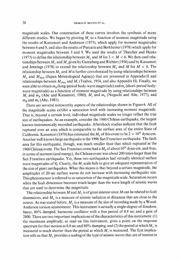
In Figure 6 we show the relationships between moment magnitude and other


magnitude scales. Our construction of these curves involves the synthesis of many

different studies. We began by plotting M s as a function of moment magnitude using

the results of Kanamori and Anderson (1975), which apply for moment magnitudes

between 6 and 9, and also the results of Purcaru and Berkhemer (1978) which apply for

moment magnitudes between 3 and 9. We used the results of Thatcher and Hanks

(1973) to define the relationship between ML and Mfor 3 < M < 6. We then used rela-

tionships between ML and Ms given by Gutenberg and Richter (1956) and by Kanamori

and Jennings (1978) to extend the relationship between ML and M for M < 6. The

relationship between ML and M is further corroborated by using relationships between

ML and MjMA (Japan Meterological Agency) that are presented in Appendix II and

relationships between MjMA and Ms (Tsuboi, 1954, and also Appendix II). Finally, we

were able to obtain m~ (long-period body-wave magnitude) and m b (short-period body-

wave magnitude) as a function of moment magnitude by using relationships between Ms and mB (Abe and Kanamori, 1980), Ms and mb (Noguchi and Abe, 1977), and

me and m b (Abe, 1981).

There are serveral noteworthy aspects of the relationships shown in Figure 6. All of

the magnitude scales exhibit a saturation level with increasing moment magnitude.

That is, beyond a certain level, individual magnitude scales no longer reflect the true

size of earthquakes. As an example, consider the 1960 Chilean earthquake, the largest

known instrumentally recorded earthquake. Aftershock studies indicate that the fault

ruptured over an area which is comparable to the surface area of the entire State of

California. Kanamori (1978) has estimated the M0 of this event to be 2 x 103o dyne-cm.

Another well known large earthquake is the 1906 San Francisco earthquake. The fault

area for this earthquake, though, was much smaller than that which ruptured in the

1960 Chilean event. The San Francisco event had aM0 of about 10 28 dyne-cm, and thus,

in terms of moment (and energy), the Chilean event was about 200 times larger than the

San Francisco earthquake. Yet, these two earthquakes had virtually identical surface

wave magnitudes of 8�88 Clearly, the Ms scale fails to give an adequate representation of

the size of giant earthquakes. What this means is that beyond a certain magnitude, the

amplitudes of 20-sec surface waves do not increase with increasing earthquake size.

This phenomenon is referred to as saturation of the magnitude scale. Saturation occurs

when the fault dimension becomes much larger than the wave length of seismic waves

that are used to determine the magnitude.

The relationship between M and M L is of great interest since M can be related to fault

dimensions, and ML is a measure of seismic radiation at distances that are close to the

source. As was stated before, ML is a measure of the size of recording made by a Wood-

Anderson torsion seismometer. This instrument is actually a single-degree-of-freedom,

linear, 80% damped, harmonic oscillator with a free period of 0.8 sec and a gain of

2800. There are two important implications of the characteristics of this instrument: (1)

the maximum amplitude, as read on this instrument, gives a point on the response

spectrum for that motion at 0.8 sec and 80% damping, and (2) the period at which ML is

measured is much shorter than the period at which Ms is measured. The first implica-

tion tells us that ML provides a scaling of the type of seismic waves that are of interest in


earthquake engineering. The second means that we should expect a saturation of the

local magnitude scale even before M s saturates. Since we intend to use M L in our

procedure for estimating ground motions, the saturation level of ML is of keen interest.

We give a more detailed discussion of this problem in het next section.

There are several other noteworthy features of Figure 6. We can see that both mB

(long-period body-wave magnitude) and MjM A give a fairly good indication of the size

of earthquakes having moment magnitudes less than 8. Both of these scales are based

upon measurements of peak amplitudes of waves with periods between 5 and 10 sec. rn B

is important since it is available for many older earthquakes (see Abe, 1981). Unfortu-

nately, it is not available for most recent events. Due to changes in instrumentation in

the 1960's, the rn B scale was replaced by themb scale, rn b is based on the amplitude of the

initial several seconds ofteleseismic body waves with periods near 1 sec. Unfortunately,

rn b does not seem to give a very good indication of earthquake size.

2.2 . IMPLICATIONS OF THE LOCAL MAGNITUDE SCALE

Although the My scale was originally developed to measure the overall size of

earthquakes, it has become clear that My is well suited to measure the relative sizes of

strong ground motions. As a part of the guidelines, we use M L to scale strong motion re-

cords in a very direct manner. A modified version of Richter's original distance

function is used to scale records with distance. Records are scaled according to

earthquake size by using the definition of the magnitude scale directly. Site effects (the

effects of local soils) are included by introducing an appropriate correction factor.

Local magnitudes are related to fault dimensions by simple relationships that can be

derived from dislocation theory. It is important to recognize that the M L scale is not a

panecea. Most of the problems that are associated with understanding the motions that

are produced by a particular earthquake still exist. The conceptual simplicity that

results from using the local magnitude scale to estimate response spectra is the major

motivation for incorporating local magnitude into our procedure for estimating

ground motions.

The definition of local magnitude is,

ML = Log Awa - LogA 0, (16)

where A,, a is the maximum trace amplitude on a Wood-Anderson (horizontal) seismo-

meter, and A 0 is a distance correction which will be discussed shortly. Now if the

displacement response spectrum of a motion is given by S d (z, ~), where z is period, and

is the damping fraction, then

Sd(t = 0.8, ~ = 0.8) = Aw,/2800, (17)

where the factor of 2800 is included to correct for the gain of a Wood-Anderson

seismometer. Combining Equations (16) and (17), we obtain

Sd('r = 0 .8 , ~ = 0 . 8 ) -- AO IoML 2800 (18)

4 0 THOMAS H. HEATON ET AL.

75

6,5

5 . 5

I ' ' ' l i ' ' ' l ' ' ' I

�9 t

�9 �9

' i i i i

S o n F e r n o n d o 9 Feb. 1971

L .~ �9 , , �9

I I I i [ t I I i | l , i I l I i I I I ' I I I

50 I00 km 150 200

7.5

6.-~

" Imperial Valley 15 Oct. 1979

�9 s =, , . ~ " ~ = �9 I . ; " mean = 6.4 s.d. = 0.25

, , , , l i i , , I , , , , I i i , i I I I i I

50 I00 km i50 200

8.0

7.0

6.C

I ' ' I I = i i I = = i

Borrego Mtn. 9Apri l 1968

m e a n = 6 . 9 2 s . d . = 0 . 1 4

. i

= ~ , = I i i i i I i i L , I , i i i I i J = ,

50 100 km tSO 200

8.0

7.0

6.0

' ' I ' ' ' I ' ' I ' ' l I i i I

K e r n County 2I July 1952

; m e a n = 7 . i 9 s . d , = 0 . 1 8

i i I I I I I i 1 J i i i I I I i I [ I J '

50 I00 km 150 200

7s

613.

5.C

I

i = l J I l l

Lytle Creek I Sep. 19

m e a n = 5.78 s.d. = 0.15 ,, i

�9 , % -

, , , ~ I i i I a I I I I I I a I I I I I

50 IO0 km 150 200

Fig. 7. Values of local magnitude plotted as a function of distance for several California earthquakes. Lines

indicate mean values and + one standard deviation. The modified distance at tenuation factor o f Jennings

and Kanamor i (1982) was assumed and data were taken either from Kanamori and Jennings (1978) or were

new data used with the permission of Kanamori and Jennings.


For periods near one second, there is a general correspondence between response

spectral level and the peak velocity of the ground motion. In fact, the output of a Wood-

Anderson seismometer usually looks very similar in character to records of ground

velocity. Thus, the local magnitude scale can be thought of as a scaling relationship for

ground velocity. We must now address some important, but difficult, questions

concerning the local magnitude scale. How well does the local magnitude scale work

when scaling strong ground motions? How well can we estimate the relationships

between fault dimensions and local magnitudes? Before discussing these problems, we

warn the reader that a full resolution of these questions has not, to date, been possible.

Kanamori and Jennings (1978) have studied the local magnitudes of the larger

earthquakes in the western United States, and their results demonstrate the feasibility

of using local magnitude as a scaling relationship for strong ground motions. Notice

that Equation (16) indicates that the correction for the decay of amplitude with

distance is not a function of magnitude. Since Richter originally derived this relation-

ship using small earthquakes, it is not clear whether it also applies to large earthquakes.

Kanamori (1978) has pointed out that 'it is possible that, for very large earthquakes,

complex interference of seismic waves originating from different parts of the fault plane

may significantly affect the decay rate of the maximum amplitude resulting in distance

dependent ML'.

Figure 7, which was constructed from studies by Kanamori and Jennings (1978) and

Jennings and Kanamori (1982), shows the value of ML as a function of distance for

several well-recorded California earthquakes. The values o f M L are defined according

to the definition given in Equation (16). However, we have used a distance attenuation

factor which Jennings and Kanamori (1982) modified from the original one given by

T A B L E 1

Local magnitude distance at tenuation factor

(modified by Jennings and Kanamori , 1983)

Distance (kin) - Log A o Distance - Log A o

0 1.4 120 3.1

3 1.5 140 3.2

6 1.6 160 3.3

9 1.7 180 3.4

12.5 1.8 200 3.5

16.5 1.9 220 3.6

21 2.0 240 3.7

26 2.l 260 3.8

31 2.2 280 3.9

37 2.3 300 4.0

43 2.4 320 4.1

51 2.5 340 4.2

60 2.6 360 4.3

70 2.7 380 4.4

80 2.8 400 4.5

90 2.9 450 4.6

100 3.0 500 4.7

42 T H O M A S H . H E A T O N ET A L .

o <~

o

i

5.0

2 . 0

i .O 0

, i , i i I , I , I ~ I = I , j . . , . . p _ ~ . T . . ~ - .

. - " d e n n i n g s a n d .

J , . . o , . , " K o n o m o r i ( 1 9 8 2 )

, i , I , I , I i i , I ' I , I ~ I = I0 20 30 40 50 60 70 80 90 I'

D i s t 0 n c e , k m

5.0 ' I i I I I i I , i I ! I I I I I I !

4.0

5"(~00 200 500 400 D i s t a n c e , k m

] i !

500

Fig. 8. Distance attenuation laws for local magnitude scale. Dotted line signifies the attenuation law originally proposed by Richter (1958) and the solid line is the modified attenuation law proposed by Jennings

and Kanamori (1982).

Richter (1958). Both the original and modified distance attenuation curves are shown

in Figure8. In Figure7 we see that there are not obvious systematic trends with

distance, indicating that the modified attenuation curve is appropriate for strong

motion scaling purposes. This new attenuation curve is als0 compatible with recent

simulation studies conducted by Hadley and Helmberger (1980). Throughout the

remainder of this study, we will assume that the modified attenuation curve is more

appropriate for scaling strong motions. Table I gives values of Log A 0 as a function of

distance.

Figure 7 also shows the scatter typically encountered in the measurement of local

magnitudes. The degree of scatter for these larger events is not significantly larger than

that encountered when studying the local magnitudes of small earthquakes. It should

be remembered, however, that the local magnitude scale is logarithmic, and a factor of

2 in amplitude corresponds to a difference in magnitude of only 0.3 units.

At this point, it is instructive to compare the distance scaling in the local magnitude

scale with some of the familiar distance scaling laws that have been traditionally used in

ESTIMATING G R O U N D MOTIONS U S I N G R E C O R D E D A C C E L E R O G R A M S 43

Fig. 9.

OJ 0

E

i .r

P 0

0 0

,,r

0

t t

0 - J

! I

- - i l

I I ! I I I I [ I I I I I | I I i i I I I I I I I I I

- - MLdennings and Kanarnori -(198?-)

. . . . . . . . M L Richter (1958) D0n0van(1972)

Schnabel and Seed(1975)

"-,-. ~ ,,.,., ~ ~176

, ,

1

R

J Majority of

the Data

\ \

\

m

l l ~ i ~ 1 i I ~ t i t I I I I t I 1 I I ! I I I I I

0 I 2 5

LooA, km

Comparison of different distance attenuation laws for M 6-1/'2 earthquakes (modified from Trifunac and Brady, 1976).

earthquake engineering. Figure 9 shows the distance scaling for M L along with a variety

of other distance scaling laws. Several of these other scaling relationships are for peak

acceleration, whereas M L is more related to a peak velocity relationship. Kanamori and

Jennings (1978) were not the first to use local magnitudes in the scaling of strong

ground motions. Trifunac and Brady (1976) also used Richter's distance scaling law to

scale strong motions with distance. Figure 9 is a modification of Figure 1 in Trifunac

and Brady's (1976) paper. A detailed inspection of Figure 9 shows some interesting

differences between the ML scaling and other scaling relationships. Although all of the

curves pass through the bulk of the data, Richter's original curve shows a generally

higher rate of attenuation in the distance range of 20 to 200 km than the other curves

44 T H O M A S H. H E A T O N ET AL.

do. However, in this same distance range, the modified ML attenuation law shows an at-

tenuation rate that is compatible with the attenuation law for ground velocities

proposed by Espinosa (1977). This observation further supports the use of the modified

M L attenuation curve. Although the modified ML curve shows a more gradual

attenuation than the original between 20 and 200 kin, it does attain the same high value

for zero distance as Richter's original. This value is significantly higher than that

predicted from Schnabel and Seed's (1973) or Donovan's (1972) acceleration attenua-

tion curves. However, the scatter in the data is quite large and there are still relatively

few data available at very small distances. At present, it does not seem possible to verify

the level of shaking that is predicted by the M r scale at very small distances. However,

new data from the 1979 Imperial Valley earthquake tends to support the hypothesis

that the ML distance attenuation curve is indeed appropriate for very small source

distances and moderate sized earthquakes. Papers by Trifunac and Brady (1976) and

Trifunac (1976) contain enlightening discussions on the use of Richter's distance

scaling law.

We now comment on the way in which local magnitude scales amplitude with

magnitude. By the definition of local magnitude (Equation (21)), the peak amplitude,

as recorded by a Wood-Anderson torsion seismometer, depends exponentially on the

local magnitude. That is, for each unit increase in ML, the response spectrum at 0.8 sec

for 80% damping increases by a factor of 10. Although this is a statement of the

obvious, the implications are significant. In Figure 10, the expected peak amplitude of a

Wood-Anderson recording (approximately related to the peak ground velocity) are

plotted as a function of magnitude and distance. For comparison, Schnabel and Seed's

(1973) estimation of peak acceleration, as a function of magnitude and distance, is also

shown. The difference in the nature of these curves is striking. Not only are the distance

attenuation curves different, but the peak accelerations clearly do not depend on

magnitude in an exponential fashion. There is a variety of explanations for this.

The first thing to remember is that the local magnitude scale saturates before the

surface wave magnitude scale does. Schnabel and Seed's curves are given as a function

of Ms, and for magnitudes of 6-1/2 and above, the local magnitude scale does not give a

good representation of the overall size of the earthquake. This point was discussed in

the last section. Also, Schnabel and Seed's curves are for peak acceleration which is a

measure of the amplitudes of high-frequency waves generated by the earthquake. The

same phenomenon that is responsible for the saturation of M L also causes the peak

acceleration to saturate, but at a lower magnitude. Trifunac (1976) documents the fact

that peak accelerations are a weaker function of earthquake size than peak velocity.

Finally, the relationships shown in Figure 12 are basically empirical in nature. Since

there are very few data at small distances or from large earthquakes, both of these sets

of curves could be inappropriate for small distances or large earthquakes. In fact, there

is good reason to suspect that the ML scaling law may not be appropriate at small

distances and for ML's above 6-1/2. This can be seen best by examining the local

magnitudes of the 1971 San Fernando earthquake. Kanamori and Jennings (1978)

determined that the M L of this earthquake was 6.5. They also found that the accelero-


106 ' ' . . . . ' ' l I I i I I I I I J I I I I I I I I

E . ~ . . 0 . . - ~ " ~ - ~-Limit of Applicobllity 1 E ~ for M L @

to 5 Ioo

e- ~ % %

I �9 '~ "~ % r

" 0 ',~ 0 % % r

�9 %% . 10 4 - . . I0 a.

I I0 I 0 0 I 0 0 0 A, km

Fig. 10. Scaling of peak amplitude as measured on a Wood-Anderson torsion seismometer as a function of M L and distance (modified distance attenuation curve assumed). Schnabel and Seed's (1973) scaling of peak acceleration with distance and magnitude (unspecified, but assumed to be Ms) is shown for comparison.

graph recording from Pacoima Dam, the station closest to the epicenter, indicated a

local magnitude of 6.5. Kanamori and Jennings (1978) also calculated ML for the 1952

Kern County earthquake and found it to be 7.2. If the Pacoima record is representative

of the motions to be expected in the nearfield from an M L 6-1/2, then what motions

would we expect in the nearfield of an ML 7.2? Taken at face value, the logarithmic

scaling associated with ML would indicate that motions in the nearfield of the Kern

County earthquake were about five times those recorded at Pacoima Dam in 1971.

Since the Pacoima motions were some of the most violent ever recorded, it does not

seem likely that the Kern County motions were five times larger.

How large can the motion be in the nearfield? Of course, this is a question that cannot

presently be answered. However, based on some rather crude, but straightforward,

source models, Brune (1978) has concluded that ground velocities of order two meters

per second could be expected in the nearfield of some large earthquakes. Although

46 THOMAS H. HEATON E'f AL.

Brune's estimate is defendable, based on the present knowledge of earthquake sources,

there are far too few data and too much uncertainty in faulting parameters to access ful-

ly the significance of Brune's calculations. In fact, there is not sufficient control on

faulting parameters to rule out the possibility of motions large enough to yield a local

magnitude of 7 in the nearfield. However, building damage observed near large

earthquakes has usually not been as great as engineers would have expected for such

large velocities. Even this observation is complicated by the fact that the local

magnitudes of most large earthquakes are lower than 7, and thus, the macroseismic

effects of the nearfield motions, due to an earthquake with a local magnitude of 7, are

rarely observed.

We have reached an impasse. The local magnitude scale predicts very large motions

in the nearfield of earthquakes with high local magnitudes, and these large motions

cannot be summarily discounted on the basis of theoretical seismological considera-

tions. However, these large motions do not seem to be consistent with the observed

damage of large earthquakes. Due to a lack of data, the problem of the sizes of motions

in the nearfield of a larger earthquake (in the sense of ML) is unresolved. However,

based on observations of macroseismic effects, it is our opinion that the ML scale is

inappropriate to scale the nearfield motions of earthquakes with ML greater than 6-1/2.

In addition, it seems unlikely that future nearfield recordings will yield an ML greater

than 6-3/4. Because of our poor understanding of very nearfield motions from large

earthquakes, we have included a limit on the range of applicability for the curves shown

in Figure 10.

2,3. ESTIMATION OF LOCAL MAGNITUDE

We have discussed how the overall size of an earthquake can be estimated through the

use of seismic moment. We also discussed how the local magnitude scale can be used to

scale the sizes of strong ground motion. Furthermore, we demonstrated that there is a

general relationship between local magnitude and seismic moment. In this section, we

refine the relationship between local magnitude and seismic moment by including

considerations of tectonic setting and local site conditions.

Up to now, we have stressed the relationship between M L and the earthquake source.

We assumed that distance was the only parameter that needs to be considered other

than the source characteristics. However, it is clear that the nature of the observed

motions also depends on the velocity structure of the medium through which the waves

travel. The effects of the travel path are so complex and varied, that a complete

parameterization of the problem appears impossible. It is possible, however, to

parameterize at least a small portion of thi~ problem in a rather simple way. The

conditions of the local soil can be characterized by estimating the stiffness. In this

study, we will use the following convention: 0 represents soft alluvium deposits, 2

represents basement or crystalline rocks, and 1 represents an intermediate condition

such as sedimentary rocks. This particular soil classification is explained more fully by

Trifunac and Brady (1975). Although more elaborate soil classifications have been


devised, it seems rather pointless to give a detailed parameterization of the soils when so

many other physical parameters are ignored. As could be expected, the great variation

in other physical parameters tends to obscure the relationship between the amplitudes

of ground motions and the local soil conditions. In general, it appears that soft soils

produce larger ground motions. Trifunac (1976) has studied this in some detail and he

found that this effect is frequency dependent. He found the weakest correlation existed

for peak accelerations, while the strongest correlation existed for peak displacement.

Most of the data used in Trifunac's (1976) study was recorded during the 1971 San

Fernando earthquake. Liu and Heaton (1984) studied the strong-motion waveforms of

this event and concluded that the excitation of surface waves in large sedimentary

basins is the principle reason why soft sites recorded relatively larger long-period

motions than bedrock sites. Trifunac's study of peak velocity suggests the following site

correction for the local magnitude scale; add 0.15 for sites designated 0, do not correct

sites which are designated 1, subtract 0.15 for sites designated 2.

It is interesting to note that most accelerograms (approximately 2/3) have been

recorded on sites which are classified as soft alluvium. We consider our uncorrected-

sites to be intermediate sites and, since Kanamori and Jennings (1978) did not apply site

correction factors in their computation Of ML, their values are systematically higher (by

about 0.1 unit) than those which would be computed using a site correction factor.

Earlier, we pointed out that there is both theoretical and empirical justification for a

saturation of the local magnitude scale for earthquakes beyond a certain size. The level

at which the local magnitude scale saturates is an issue of central importance in the

estimation of strong ground motions. In Figure 4, we showed the empirical relationship

between Ms and ML which was derived from the data sets of Gutenberg and Richter

(1956) and Kanamori and Jennings (1978). A local magnitude of 7-1/4 (Kern County

earthquake) is presently the highest M L recorded. If we assume that Kern County is

fairly typical ofintraplate (high stress drop) earthquakes, and if we account for the fact

that 7-1/4 represents values measured on soft soil sites, then we would recommend a

saturation value of 7.1 for intraplate earthquakes with sites having intermediate site

conditions.

In Appendix I we investigate hypothetical fault models to deduce that the saturation

level of different magnitude scales should be proportional to Log Act (Equation 0.32)).

This relationship is in agreement with the notion that the average dislocation velocity is

proportional to stress drop. If ground velocity is linearly related to dislocation

velocities, then we expect the saturation of ML to depend on Log A~. Thus if we assume

that ML = 7.1 represents the average local magnitude saturation of intraplate earth-

quakes with stress drops of about 60 bars, one would expect interplate earthquakes

with 30 bar stress drops to have an average local magnitude saturation level of about

6.8, and the average local magnitude saturation level of shallow subduction-zone

events would be about 6.5 since their average stress drop appears to be about 15 bars.

These values assume intermediate site conditions.

In Appendix II, we compare strong ground motions recorded in Japan with those

recorded in the western U.S. We find that the distribution of available Japanese records


with respect to earthquake magnitude and site distance is markedly different from the

distribution of U.S. records. In contrast to U.S. records, there are few Japanese records

available at small distances from moderate to large earthquakes. There are, however,

many recordings of large off-shore Japanese subduction zone earthquakes that are

taken at large distances. Despite the difference in distribution of available strong

motion records and the obvious difference in tectonic setting, we find that when ground

motions observed at comparable site distances and earthquake magnitudes are com-

pared, Japanese and U.S. motions are remarkably similar. Calculation of the local

magnitudes of large Japanese subduction zone earthquakes indicates a local magnitude

saturation level of about 7-1/4. This value is comparable to the value we deem

appropriate for intraplate crustal events. This seems to contradict our speculation that

subduction zone earthquakes should exhibit a relatively lower magnitude saturation

level due to their lower average stress drops. However, average stress drop is not the

only source parameter that is significantly different when comparing large crustal and

subduction zone earthquakes. Subduction zone earthquakes may have both large fault

lengths and widths, whereas crustal earthquakes may have large fault lengths, but the

fault widths are limited. In general, a recording site is most affected by that part of the

rupture that is closest to it. Thus, we generally expect long, narrow faults to have

relatively less area of faulting nearby to any site than does a nearly square fault. Also,

square faults produce larger dislocations than long, narrow faults of equal area and

stress drop (Equation (11)). For these reasons, we expect subduction zone events, with

8 ' ' ~ ' ' ' ' ' ' 1 ' ' ' ' ' ' ' ' ' 1 ' ' ' ' ' ' ' ' ' 1 ' ' ' ' ' ' ' ' ' 1 ' ' ' ' ' . . . . I . . . . . . . . .

( I n t r a - P l a t e E~ Subducting Margin)

7 ( T r a n s f o r m M a r g i n )

ML

6

5

, , , , , , , , I , , , , , , , , , I , , , , , , , , , I , , , , , , , , , I , , , , , , , , , l , , , , , , , ,

4 5 6 7 8 9 I0

M o m e n t M a g n i t u d e , .M.

Fig. 11. Assumed average relationship between local magni tude and moment magni tude for three different

tectonic regimes.


their relatively large fault widths, to have higher levels of local magnitude saturation

than events with long, narrow faults and equal stress drops. Exactly how stress drop

and fault aspect ratio trade off is not presently understood. However, evidence

presented in Appendix II, supports the local magnitude saturation of about 7-1/4 for

subduction zone events. As we pointed out in the last section, there are reasons to

believe that the local magnitude distance attenuation curve may not be appropriate for

very large earthquakes and small source distances. We can anticipate that fault aspect

ratio will be an important parameter in the solution of this problem.

In this study, we will assume that the basic relationship between moment magnitude

and local magnitude is the one that is shown in Figure 11. It is derived from empirical

data, Equation (I.32), and the arguments just given. It is important to recognize that

both our data and our source theory are quite limited. Thus, this relationship must be

considered to be a crude hypothesis that includes stress drop, a parameter which the

study of simple source models indicates is of fundamental importance in the scaling of

seismic radiation. It is also important to recognize that our understanding of the stress

drop of earthquakes is fairly limited. Stress drop cannot be measured directly and must

instead be inferred from estimates of fault slip and fault dimensions. Kanamori (1980)

has summarized many of the important studies of the state of stress in the earth's

lithosphere. Figure 12 is taken from his paper and shows the calculated stress drops of

I06 I I I I I I , I l �9 Inter-Plate

o otra a,e 10 5 _ .\

t%1

E

&

10 4

3 I0

5

0 =1"25 x 1022 S ~ dyne-cm

(S in km 2 )

i01 I / , I I I I I i I I I I

10 25 I0 26 1027 1028 i029 i030

M o, dyne-cm

Fig. 12. Relationship between fault area and seismic moment. The solid lines denote constant stress drops

and the dashed line (M 0 = 1.23 x 1022 S 3/2 dyne-cm; S in km 2) signifies a stress drop of about 30 bars. Solid

points denote interplate earthquakes and open circle denote intraplate earthquakes. This figure is taken from

Kanamori (1980) and is used with permission from the author.


well-studied earthquakes as a function of earthquake size. It is clear from Figure 12 that

stress drop is not a parameter which can be accurately predicted. However, it is of such

physical importance that an understanding of the strong ground motions would be very

difficult without it. Thus, the relationships given in Figure 11 are our attempt to include

stress drop in an average way.

3. Seismic Design Guidelines

3.1. GUIDELINES FOR ESTIMATING THE MOTIONS FROM SMALL AND MODERATE

EARTHQUAKES

In the previous sections we concentrated on understanding the sizes of earthquakes, the

scaling of strong ground motion, and the relationships between earthquake siz e and the

amplitude of strong ground motion. In this section we demonstrate a technique for

estimating ground motion time histories based on estimates of fault dimensions and

tectonic setting. As was stated in the introduction, we modify and expand a technique

that is described by Guzman and Jennings (1976). The basic idea is to find records from

sites with settings similar to those for the area to be studied. The local magnitude scale is

used to scale these records with respect to distance, site condition, and earthquake size.

Because of the many problems that are associated with such scaling, it is important that

we use records that require minimal scaling. Since the data set is very limited, this is not

always easy. In particular, there are no strong motion records of giant (M> 8-1/2)

earthquakes, and for these earthquakes, the procedure described in this section is not

recommended.

. From all we have said in the preceding section, it should be clear that we feel that

'merely specifying a surface wave magnitude and a distance is insufficient input to derive

the ground motions expected at a particular site. Given no constraints, what would be

the best way to estimate the future motions at a site? The most obvious answer to this

problem would be to have a collection of all the ground motions experienced by that

site over the last several thousand years. We could then forget about the difficulties

associated with understanding the physics of what controls the ground motions.

Although this solution is unattainable, it gives the basic philosophy for the procedure

we will describe. By collecting records from sites with geologic conditions that are

similar to the study site, we can incorporate important physical parameters into our

procedure in a very direct fashion. The major drawback in this procedure arises from

the limited size of our data set. By selecting sets of the data, our ability to estimate the

statistical variation within that subset becomes limited. As the data set grows, this

limitation will become less important. Since the data are limited, it is possible that only

a few records will be found that are appropriate for a particular site, but it is possible to

include records taken under somewhat different conditions by scaling these records

with the relationships that have been discussed in the preceeding sections. Obviously, it

is desirable to keep such scaling to a minimum.

It is important to have access to a fairly extensive collection of strong motion data if


the procedure is to be effective. Crouse et al. (1981), have compiled an extensive

catalogue of digitized accelerograms. Nearly 1000 accelerograms from many countries

are included. This catalogue is probably unique, since it contains information about

site conditions and also seismological information for causative earthquakes. Al-

though this is the most complete strong motion catalogue that we know of, it should not

be considered exhaustive. Furthermore, in our opinion, some of the parameters listed

should be considered prelimary estimates. Therefore, it is recommended that a more

detailed investigation of the characteristics of each earthquake be conducted for those

records that are proposed for use in the design of important facilities.

The first task is to decide which records are appropriate for a particular site. The

basic input parameters will be: (1) source dimensions, (2) distance from rupture, (3)

tectonic setting, and (4) site conditions. Ideally, it would be nice to sidestep the problem

of using magnitude as an estimate of earthquake size, and to use source dimension

directly by simply finding those earthquakes with similar source dimensions. Unfortu-

nately, the source dimensions of most earthquakes have not been well studied, and the

magnitude scale must be used to estimate the overall size of an earthquake. As

previously discussed, it is our opinion that moment magnitude is the best way to

estimate earthquake size at this time. Given the fault dimensions, Equation (15) can be

used to estimate the expected moment magnitude.

Records taken at similar distances from earthquakes of similar seismic moments can

be found by studying Figure 13. In this figure, we have plotted each of the records found

91 , 6.8

8l 9 ~176

~ . �9 ~ . ~ . ~ ' . ~ i " ~ -

N

s 4 . :'

2'o 4o 6'o 8'o ,6o ,~o ~o ,~o

~zO 0

Distan e ~. km

6.8

6.75

" -6.6

~0"._....~L.3~.6. 4

. . 8.0

100 r

5.0

40

180 2 0 0

Fig. 13. Records from Crouse et al. (1981), catalogue plotted as a function of distance and magnitude.

Contours denote theoretical lines of equal peak amplitude (milimeters) on a Wood-Anderson torsion

seismometer, assuming that the vertical scale is approximately equal to moment magnitude and the stress

drop is 30 bars.


in the Crouse et al. (1981), catalogue as a function of magnitude and distance. Although

the magnitudes plotted are not moment magnitude, some care was taken to choose the

magnitude value that was not affected by the saturation phenomenon which was

described earlier. Notice that all of our records are for earthquakes with moment

magnitudes of less than 8.

Also shown in Figure 13 are contours of equal local magnitude scaling, that is, equal

peak amplitude as measured on a Wood- Anderson seismometer. These contours are

for an average stress drop of 30 bars, and can be derived directly from our hypothesized

relationship between local magnitude and moment magnitude, which is shown in

Figure 11, and from the modified version of Richter's original distance attenuation law,

which is shown in Figure 8. Records that fall along the same contour should have

approximately equal peak spectral velocity.

We will now describe the procedure that, in our opinion, is appropriate for obtaining

the ground motions which can be expected at a particular site.

( 1 ) Characterize the source type and tectonic setting.

( 2 ) Determine the dimensions of the expected rupture surface, and then calculate a

moment magnitude using Equation (15).

( 3 ) Determine the closest distance from the site to the rupture surface.

( 4 ) Determine the site conditions (soft, intermediate, and hard) (Trifunac and Brady,

1976).

5) Determine ML (site) for postulated earthquake by using Steps 1 and 2 and Figure

11.

6) Determine site correction factor Cs, where C, = 0.15 for soft, 0 for intermediate,

and - 0.15 for hard.

7) Determine distance correction A 0 (site) using Figure 8.

8) Compute expected amplitude on a Wood-Anderson seismometer using the for-

mula,

A (site) : ao i0 (ML-~ Cs) (19)

9) Search the Crouse et al. (1981), catalogue for records taken at similar distances

and with similar magnitudes and tectonic settings. Choose as many records as

possible. Index the records i= 1 . . . . n.

(10) For each earthquake, determine a moment magnitude. Use either published

estimates of seismic moment or convert other magnitudes to moment magnitude

using Figure 6.

(11) For each record, determine an No L using the estimated moment magnitude of the

earthquake and Figure 11.

(12) Determine site correction factor CI. for each record.

(13) Determine distance correction factor A; for each record; use figure 8.

(14) Compute expected amplitude on a Wood-Anderson seismometer for each record

using the formula,


A' = A; 10/MI + <). (20)

(15) Multiply the ith record by the scaling factor si, where

S i = A(si~e) A' (21)

The end result of this process is a suite of n records that should be representative of

the types of motion that could be expected at the study site. Since the scaling process is

not well understood, it is desirable to use records that require as little scaling as is

possible. As Guzman and Jennings (1976) stated, 'the final product of the scaling

procedure is only dependent on relative values, not on the absolute values of accelera-

tion' (amplitude on a Wood-Anderson seismometer for this procedure). This means

that the scaling factors depend primarily on the shapes and relative amplitudes of the

attenuation curves for different magnitudes.

We now give an example of how this procedure can be used to obtain a free-field

design spectrum. In this example, we assume a site that lies at a distance of 50 km from a

strike-slip fault that has dimensions appropriate for producing an earthquake with a

moment magnitude of 6-1/2. We will further assume that the study site is of intermedi-

ate hardness. Figure 13 shows that there are a number of records that could be included

in our suite of records. We use the fifteen records (thirteen western United States and

two Japanese) listed in Table II as our set of analogous records. We have also used the

steps outlined previously to compute a scale factor for each record. Notice that only

records with scaling factors of less than 2 have been chosen. Also listed are both the

scaled and unscaled average peak horizontal ground velocities. If the unsealed veloci-

ties are averaged over all records, then we obtain a value of 14.3 centimeters per second

(cm sec -1) with a standard deviation of 8.5 cm sec-1. The scaled velocities, however,

scatter less and yield an average value of 17.9 cm sec- 1 with a standard deviation of 9 cm

sec -1. The highest scaled velocity is 35.1 cm sec -1, and the lowest is 3.6 cm sec -1.

Although this variation may seem large, it reflects the true uncertainty in the answer

given our present level of understanding of earthquake motions.

It is worth noting that both the highest and lowest scaled average peak velocities in

Table II were produced by a single earthquake, the 1979 Imperial Valley earthquake.

The difference in peak velocities between stations at Delta and Plaster City is nearly an

order of magnitude. Yet both stations are located within the Imperial Valley at roughly

comparable distances from the earthquake rupture. Although there are undoubtedly

good physical explanations for this difference, it probably would have been quite

difficult to predict this result. It is also worth noting that the third highest and second

lowest velocities are from two records which were also produced under nearly identical

circumstances. That is, records # 4 and # 8 are both from the station at E1 Centro,

California, and were produced by M s 6-1/2 earthquakes on the Coyote Creek fault. In

fact, the two earthquakes (1942 Borrego Valley and 1968 Borrego Mountain) occurred

very close to one another. Nevertheless, the E1 Centro records from the closer 1942

earthquake are much smaller than the records from the 1968 earthquake. A close

5 4 T H O M A S H . H E A T O N E T A L .

<

<.='~

�9

I

o=

o

�9

z ~

6 z

o o

t'-q r c q r ~ ~ t",l t",l r ~ ~ ~

06

§

t r ] ~ t"q qD OO t"q t ' q t"q t"'-- ~"x t-~ ~ ~'~

~ ~5 ,.6 ..6 ,---; ~ r--: c5 ~ ~ o ,'.-; ,.6 ~: <5 "4

+ + + + + + + I + + + + + + §

o ~ - t 0 0 I

~ L I00[ 1968 Bo~rego Mtn.

-~~176 lt - 2 0 0 ' , , , , , , , , , , , , , , , ,

E S T I M A T I N G G R O U N D M O T I O N S U S I N G R E C O R D E D A C C E L E R O G R A M S

North Component of Ground Me, ions Recorded at El Centre

1

>

2C

IC

o

-IC

-2c

4c

1942 Borrego Valley

~~"~ "vY TM "W~ "V\/ ~ / V~ W ~ ~ v \

1968 Borrego Mtn. 2C

-2C J~

- 4 0 _ _ , , , , , i L b , i i ~ i i i i i

55

1942 Borrego Valley

- v y V j v

-(

E

--~ 12

4 / o ~ _ _ j V \ , , ,, / ~

-4 y -6

-12

- ~ d - - " ~ ' n'6 ' ~'4 ' 3'2 ' 4'0 ' 98 ' g ' s'4 ' -r~ T ime,seconds

Fig. 14. North component of ground motion for two M 6-1/2 Borrego, California earthquakes as recorded

at E1 Centro. Note that the 1942 records are plotted on an amplitude scale half as large as that used to plot the

1968 records.


inspection of the motions produced at E1 Centro by those earthquakes reveals striking

similarities and differences. The long-period surface wave parts of the records are very

similar and yet, the higher-frequency acceleration time histories are very different. This

can be seen in Figure 14 that shows the processed records of the north component of

motion recorded at E1 Centro for the 1942 and 1968 earthquakes. The exact causes for

the differences between the records in Figure 14 are a matter of future study. However,

there is presently an important lesson to be learned from these records. Although we

may approximately scale for site effects, source dimensions, travel path, and tectonic

setting, there are also very important indeterminate parameters associated with the

earthquake source.

In Figure 15, we show the scaled response spectra (3% damping) for the horizontal

components of records in our suite. In general, the scatter is about an order of

magnitude. Furthermore, records that have the largest values at high frequencies may

have relatively small values at low frequencies. Although this large scatter may not

Fig. 15.

I000.

Damping = 5 %

! I I I I I I I l I i l I I E l .

, o o ^

P

U

,:. LO. A _,

\

i i J I i J I i I I l I I I l l

0.OI 0.1 I. 10.

Period, seconds

Response spectra (3% damped) for horizontal components of 15 records from strike-slip

earthquakes which are scaled to a distance of 50 km and a magnitude of 6-1/2.


U 0

E 0

r 0

I000.

I00.

I0.

�9 w J v i w �9 u l � 9 1 4 9 u

Damping = 3%

~ e

" :

/ / ' /

,//

X/P / /

y

�9 I I I a g i u i i m i �9 �9 . | , .

o.ol b.i io. Period, seconds

Fig. 16. (a) Average spectrum, (b) average plus one standard deviation spectrum, (c) spectrum of the largest single record, (d) spectrum which envelops all others; based on spectra shown in Figure 17.

seem very satisfactory, it represents our ability to parameterize strong ground motion

in terms of magnitude, distance, soil condition, and fault type. We show an example of

how the free-field design spectrum for a M 6-1/2 strike-slip earthquake at a distance of

50 km can be chosen in Figure 16. The average spectrum, the average plus one standard

deviation spectrum, the spectrum of the single largest record, and the spectrum which

envelops all others are shown. The suite of spectra shown in Figure 15 forms the basis for these choices of design spectra.

4. Conclusions

We have presented a procedure for estimating ground motions using simple scaling of

existing recorded ground motions. The scaling procedure incorporates fundamental

seismological concepts regarding the sizes of earthquakes and the saturation of


different magnitude scales. We have seen that considerable ambiguity may be present

when the term earthquake 'magnitude' is loosely defined. We choose to define

earthquake size in terms of seismic moment. We have parameterized strong ground

motions using ML scale. We suggest that saturation of the local magnitude scale may

vary systematically with average earthquake stress drop which may in turn vary

systematically with tectonic setting. Although subduction zones may produce the

largest earthquakes, they do not necessarily produce the most intense ground shaking.

Furthermore, relatively rare intraplate earthquakes may produce relatively severe

ground motions.

The procedure we have presented conserves a meaningful measure of the uncertainty

inherent when predicting ground motions from a simple parameterization of earth-

quake size and station distance. In an example, we showed that although the scatter

may be as much as an order of magnitude, it would be extremely difficult to reduce that

scatter by a better parameterization of the earthquake source or the recording site.

Appendix I: Spectral Scaling Relations

In this appendix we discuss the relationship between earthquake magnitude and

rupture parameters for several simple models of the earthquake source. These rela-

tionships are derived from estimates of the Fourier amplitude spectra of seismic energy

produced by our simple source models.

We begin with some simple observations about the way magnitude is related to

Fourier spectral amplitude. Let us define a hypothetical magnitude scale Mr that is the

logarithm of the peak amplitude of a specified wavetrain on a seismogram produced by

a specified seismometer. Seismogram wavetrains may have a wide variety of character-

istics, depending upon the nature of the input ground motion and the response of the

seismometer. In general, we can break the problem into the following four categories.

(i) A seismogram wavetrain consists of a near monochromatic waveform. Such

waveforms are often produced by narrow-band seismometers or by wavetrains that are

well-dispersed by wave propagation. In this case, we expect the peak observed

seismogram amplitude to be proportional to the Fourier spectral amplitude of the

signal at the dominant period of the signal. Thus, we expect that

where ^ denotes Fourier transform.

(ii) A seismogram wavetrain consists of a simple pulse that is recorded by a band-

limited seismometer whose free-period is large compared to the duration of the actual

ground motion. Since the duration of the signal T L is small compared to T, we may

conclude that the seismogram in this case is simply the impulse response of the

instrument. Hence

M r ~ L o g U ( T - - ~ ) ~ L o g U ( ~ ) . (I.2,


(iii) A seismogram wavetrain consists of a simple pulse that is produced by a simple

pulse in ground displacement as recorded on a broad-band seismometer. This case may

arise when observing body waves on simple damped harmonic oscillators whose period

Tis longer than the signal duration T L. In this case, the peak seismogram amplitude is

proportional to the area of the pulse divided by its pulse width and thus,

Mr ~ Log \T~O~/TL I ~ Logl= \TLT] . ( I . 3 )

(iv) A seismogram wavetrain consists of a complex collection of randomly spaced

pulses. This case may arise when observing body waves on a simple damped harmonic

oscillator whose period T is short when compared with the signal duration TL. In this

case, the Fourier spectra of the individual pulses can be summed with random phase in

order to produce the total seismogram. The amplitude spectrum of the sum of m

impulses of random phase is simply proportional x/m. Thus, the amplitude spectrum of

the ground motion is proportional to the square root of the signal duration. Thus,

[ , - r /

Log ii.4/ Ix/TL I

Actually, real seismograms do not usually fit completely into any of these categories.

However, it is clear from the preceding discussion that a general definition of M r is

given by the following:

where 0 < ~ < 1 and ~ depends upon the type ofseismometer and wavetrain that is ob-

served.

We can now demonstrate how our generalized magnitude scale M r behaves as a

function of rupture parameters for several simple source models. First we investigate a

model that was initially introduced by Haskell (1964). This model assumes that faulting

occurs uniformly on a rectangular surface. A finite, planar fault in a homogeneous

whole-space is assumed. The receiver is assumed to be at distances that are large when

compared to the fault dimensions. Rupture initiates along a line, and the linear rupture

front proceeds along the fault length at constant velocity. The dislocation time history

for every point on the fault is assumed to be a linear ramp in time. A sketch of this fault

model is found in Figure 17. Although this is a very simple fault model, it does allow us

to demonstrate phenomena that help explain the differences between various magnitu-

de scales. The following discussion was developed by Kanamori and Anderson (1975)

and later extended by Geller (1976) and Noguchi and Abe (1977).

Let us investigate the nature of motions which are produced by the model just

described.


Fault Plone

X

y r .

_o

c)l Time

Fig. 17.

L

Rupture Front

Time History of Dislocation

for any Point on Fault

Schematic of Haskell-type fault model.

Define a boxcar function, B (t/z), as follows:

O, t/T > 0

B(t/z)=- 1, O < t/r < l

O, t/r > 1.

Furthermore, define

(1.6)

where T i and Tj are the arrival times of energy from the ith andjth corners of the fault, re-

spectively. It can be shown that the displacement history at the receiver can be

approximated by the following relationship:

U(t) ~ M o B ( t / T 1 3 ) ~ B( f /T12) ~ B(T/T) , ( l . 7 )

where M0 is the seismic moment, z is the duration of the dislocation time history and *

denotes convolution. Let M r be the magnitude scale that is defined in Equation (I.5)

and, for simplicity, let us assume that ~ = 0. Taking the Fourier transform of 0.7), we

obtain

/roT,3\ f ~ T 1 2 \ ~z Sin - - S i n ~ T ) S i n ( T )

~ . (I.8) [ ~ 1 1 3 I

T T T

We now postulate the following similarity conditions:

w ~ ~L, (1.9)

b ~ Act, (I.10)

D ~ A~, (I.11) c~L


where w is fault width, and L is fault length, and c~ is a constant which gives the aspect

ratio of the rupture surface. Relationship (I.10) is the only one that we have not yet

introduced. This relationship was introduced by Brune (1970) and it states that the

dislocation velocity is proportional to the stress drop (provided certain dynamic

conditions are met). Since D(t) is assumed to be a ramp,

D

D

and from (I. 10), (I. 11), and (I. 12), we conclude that

7: ~ Lo~ ~ M 1/3 A~7 -1/3 ~1/3. (1.13)

From the definition of T~j, it is also clear that

T13 ~ w ~ tc~ ~ Mg/3 /10 "-1/3 0~ 1/3, ( I .14)

and

T12 ~ t ~ M ~ 3 z ~ 0 - l ~ 3 ~ 2~3. ( I .15)

we can now derive the relationship between M T and moment magnitude as L increases.

We approximate the function (sinx)/x by its extremal asymptotes (= 1 i fx~0;

= 1/x if x ~ ~) . We separate the problem in the following cases.

(i) L very small and then z, T13, and T12 are small compared to T/~ and (I.8) reduces

to

M r ~ L o g M o ~ ~M. (I.16)

(ii) L becomes large enough so that r < T~3 < T/~ < TI2 and then

M r - - L o g ( M o ~ ) ~ L o g ( M ~ ' 3 A c r l ' 3 c ~ 2~3) (I.17)

M + ~Log Aa + 2Log c~.

(iii) L larger yet, z < T/Tz < T13 < Tl2 and

( M~ ) UVto " ~ (I.18) MT ~ Log TlzTI3 ~ Log ' ' '1~3~ 2~30~1'3)

�89 + 2LogAa + �89 Logcc

(iv) Finally, for L very large, T/zt < "c < T~3 < T~2 and

M r ~ Log(~M~ ~ Log Aa. (I.19)

In Figure 18, we sketch the approximate relationship between moment magnitude

and magnitude M r based on spectral amplitude at a certain period. Although this is a

very simple source model, it does illustrate several features that should be observed for

actual earthquakes. For instance, a comparison ofM~. vs M in Figure 5 shows a similar


M T

. . . . [ . . . . I . . . .

F r o.. Log hr Uni,

I I I I I

4Ao"

M T ~, LogAcr

2Ao-

Ao"

-%

I I I

M'~, 2/3 Log Mo

Fig. 18. Schematic showing the way in which any band-limited magnitude scale depends upon moment magnitude assuming a simple Haskell-type fault model and three different values of stress drop. The shapes

of the curves are given by Equations (I 16) through (I. 19).

form to the one that we just derived. We note that this model predicts that the effect of

stress drop becomes important only as our hypothetical magnitude scale begins to

saturate. We also note that both the stress drop and the fault aspect ratio are relatively

important parameters in determining the period at which saturation occurs.

Unfortunately, the model of source rupture just presented is still far too simple in

several important aspects. For instance, it has become clear that earthquake rupture is

not uniform over a fault surface. In the homogeneous faulting model just presented,

high-frequency radiation appears only at the beginning and end of the observed

motion. Real seismograms, however, are usually characterized by high-frequency

arrivals that are randomly spaced throughout the entire duration of ground motion. At

small length and time scales it may be more appropriate to characterize variations in the

rupture process with statistical parameters (Haskell, 1966; Aki, 1968; Andrews, 1980).

We now introduce a new spectral scaling law that relates source dimensions to

spectral characteristics of U. Although this law is more general than that given in

Equation (I.7), it is rather ad hoc. It also shares features of other source models in which

the rupture time and dislocation amplitude are allowed to have a specified degree of


random variation on the fault surface. Assume that

�9 / r C t l \ . / 7 c T 2 \ . / T r T 3 \

T T T

As before, assume the following similarity conditions.

where

then

w = aL,

D ~ ArTw ~ A r

denotes the averge over the fault surface. Further assume that

M o ~ {)wL ~ A o - ~ 2 L 3.

We further assume that

T 1 ~ T L ~ L ~ Mol'3 Ao--l'3 ~ -2'3,

AdlI3 AO ' - 1,3 0~1,3, Z 2 ~ w ~ ~ " 0

and

T 3 ~ D/I) ~ ~L ~ M o 1'3 Ao- 1,3 ~1,3.

(I.20)

(I.21)

(I.22)

(i 23)

(1.24)

(I.25)

(1.26)

(i.27)

T1, /'2 and T3 are similar to the corresponding variables defined in our earlier

'smooth' fault model, but are in general smaller quantities. This definition is motivated

by Haskell's (1966) conclusion that rupture heterogeneity tends to introduce more

high-frequency energy than derived from similar 'smooth' models. In our previous

model, the exponents vl, v 2 and v 3 are equal to plus one. This produces a high-frequency

spectral decay rate of T 3. As random variations are added to the 'smooth' model, these

exponents become less positive. When vl + v2 + v3 < 3/2, then the degree of

heterogeneity is high enough that infinite radiated energy is produced by this spectral

scaling law.

We now derive the scaling relationships between our generalized spectral magnitude

M r which is given by Equation (I.5) and the fault parameters, fault length, aspect ratio,

and stress drop, assuming the scaling relationships given by Equations (I.20) through

(I.27). As before, we separate the problem into 4 cases and approximate the sinc

function by its extremal assymptotes. This approximation is even more appropriate in

this model since random variation eliminates the spectral holes produced by the

homogeneous rupture model.


(i) L very small and then T~, T2 and T3 are small compared to T/~ and then

M:r ~ Log M 0 - ~Log T L

- ( 1 ~)LogMo + ~L - ~ ogAa + 3Logc~

M + ~LogAcr + Log~. (1.28)

(ii) L becomes large enough that T3 < Tz < T/Tc < T~, and then

M r - Log(M~~ \ J l v l /

(1 ~ + vi \

( 3 . ~ - v l ~ + 2Vl)Log~ (I.29)

(iii) L larger yet, T 3 < T/~z < T a < r I

Mr~ L o g ( ~ ) - ~ L o g TL

~(1 ~+v13 +v2-)L~176 -~+v~3 +v2) L~

+ 3

. .~(3-r -V2)M+(~+v~3+v2) L~

+ 3

(iv) Finally, for L very large, T/~z < T3 < T2 < T~ and

Mr~ Log T~,T~2~T;~ -~Log rc

~ ( 1 - ~ + V l + v2 + v3) L~

+ ( 2~ + 2vl 3- v2 - v3) L~

+ ( ~+vl + v2 + v3) L~

( ) (~+vl+Vz+V3) L~ 3 - r M+ 2 3

(2~ + 2Vx - V2 - V3) Log c~.

(1.31)


The value of~ depends upon the type of seismogram used to measure peak amplitude

and is, in general, also a function of T. Considering the complexity of the resulting

scaling relationships, it is not too surprising to find that the various magnitude scales in

use today are not interchangeable. One significant feature of this model of magnitude

scaling is the fact that we can explicitly determine the relationship between stress drop

and Mr simply by knowing the relationship between Mr and M. That is, in all cases

(Equations 0.28) through (I.31)) we can write,

M T ~ AM + (1 - ~A)LogAa, (I.32)

where A is a function of fault length.

As an example of our more general scaling law, we now construct a specific model

which produces a short-period spectral decay rate o f t 2. For simplicity we assume that

v~ = v2 = v3 = }. We will define ~ in a way such that it is consistent with measuring both

surface wave magnitude (~ = 0 for all T) and a broad-band body-wave magnitude (~ =

1 for T > TL and ~ = ~ for T< To). Our solution becomes

(i) L small so that T3 < T2 < T~ < T/~ and

M T ~ ~ M (M 7 approximates M,) (1.33)

M r ~ M + ~ LogAa + ~ Log~ (M7 approximates m~). (!.34)

(ii) L large enough so that ~ < T2 < T/x < T1,

M r ~ ~M + ~LogAa + ~Logc~

and M r ~ ~ M ~ + ~gLogAa + ~Logc~7

(iii) L larger yet so that T 3 < T/~ < T2 < T~

M r ~ ~M + 4 LogAa + ~ Logc~

Mr ~ -~ m + ~ Log zlc~ + ~ kog~

(Mr ~ Ms) (I.3S)

(Mr me). (I.36)

( M r - Ms) (~.37)

(M, ~ ,1@. (I.38)

(iv) Finally, L large enough that T/Tc < T~ < TE < T~

M r ~ �89 M + ~ Log Aa (Mr .~ Ms) (I.39) and

M T ~ �88 M + ~LogAa + �89 ( M T ~ mB). (I.40)

By examining these hypothetical magnitude scales and source models, we have seen

that the relationships between magnitude scales in use today and fault dimension and

stress drop are likely to be quite complex. This is consistent with the observed complex

relationships between various magnitude scales that was presented in Figure 6. The

principle conclusions to be drawn from these models are: (i) magnitude scales should

saturate at large fault dimension, (ii) magnitude scales based upon short-period

measurements should saturate before magnitude scales based upon long-period meas-

urements, (iii) the ratio of fault width to fault length can be an important source scaling

parameter, (iv) stress drop is relatively unimportant before a magnitude scale begins to

saturate, but becomes the dominant parameter after a magnitude scale saturates.

66 T H O MA S H. HEATON ET AL.

Appendix II: A Comparison of U.S. and Japanese Strong Ground Motions

The purpose of this appendix is to compare recordings of strong ground motion from

Japan with those from the western U.S. To this end, we compare peak values of ground

acceleration, velocity, and displacement recorded at comparable source distances and

earthquake magnitudes. We also compute local magnitudes of Japanese earthquakes

to study magnitude saturation for subduction zones. We have collected data from

several catalogues for this comparison. Most of the digitized accelerometer data is

listed in the catalogue of Crouse et al. (1981). Additional U.S. data are from the 1979

Imperial Valley earthquake (Brady et al., 1980a) and from the 1979 Coyote Lake

earthquake (Brady et al., 1980b). The Japanese data is primarily from Crouse et al.

(1981). C. B. Crouse of Ertec has graciously supplied listings of peak accelerations of

unprocessed accelerograms as well. Some of the values of peak ground velocity from

the 1968, M, 7.8 Tokachi-Oki earthquake are from Inoue (1983). Finally, some

unprocessed peak acceleration points from Alaska (Beavan and Jacob, 1984) are

included in the Japanese data set. Unfortunately, it is beyond the scope of this study to

provide a full catalogue of all recordings used for this comparison. We have, however,

included a listing of all Japanese records for which we computed local magnitudes

(Table III). Plots of processed records included in Table III can be found in the

catalogue compiled by Mori and Crouse (1981).

The meaning of distance between the earthquake and recording site can sometimes

be ambiguous. Most distances listed in Table III are either epicentral or hypocentral

distances. However, v)hen the earthquake dimension is large, some other measure of

distance may be appropriate. In Figures 19 through 21, we have used the closest

horizontal distance between the site and the rupture. In most instances, this means that

we used the epicentral distance. In the case of the 1968, M, 7.8 Tokachi-Oki earthquake,

we computed the closest distance to the rupture surface as defined by the locations of

the first several hours ofaftershocks. Some of the Japanese events occur at considerable

depth and in these instances, it may be more appropriate to use hypocentral distance to-

gether with a new set of distance attenuation laws. However, we found that the use of

epicentral distance for earthquakes of depths up to 50 km resulted in consistent peak

motions for both shallow and deeper (less than 50 km) Japanese earthquakes.

In Figures 19 through 21, we plot peak values of ground acceleration, velocity, and

displacement as a function of distance for Japanese and U.S. records for selected

earthquake magnitude ranges. When comparing peak values of ground motion,

regardless of earthquake magnitude (Figure 19 a and b; Figure 20 a and b; Figure 21 a

and b), we see that the distribution of observed Japanese ground motions is very

different from the U.S. ground motions. In general, the largest ground motions have

been recorded in the western U.S. at small source distances. Although there are few

Japanese records of peak acceleration greater than 0.5 g, impressively large motions

have been recorded at distances of 100 km and more in Japan. Taken at face value, this

might suggest that ground motion attenuates less severely with distance in Japan.

However, when we compare motions that were recorded at comparable earthquake

ESTIMATING GROUND MOTIONS USING RECORDED ACCELEROGRAMS

TABLE III

67

Earthquake

Distance

Site Center of

No. Epicentral energy Component Log Aw~ ML(CER) ML(Ep~

2/14/56 MjMA= 6.0 Kashiwa TK024 21 50 North 4.07

Depth = 45 M L = 6. I East 4.09

North 4.07 TK024 23 51

East 4.09

4/23/62 MjMA = 7.0 Tokachioki HK005 75 100 North 4.40

Depth= 60 ML= 7.2 East 4.49

4/30/62 MjMA= 6.5 TH030 64 69 North 3.7l Depth= 35 ML= 6.4 East 3.73

5/8/63 MjMA = 6.1

Tokai KT003 53 63 North 3.64

Depth = 40 ML= 6.0 East 3.62

North 3.34 KT001 53 63

East 3.26

8/4/63 MjMA = 5.1 KT014 35 52 North 3.63 Depth= 39 ML= 5.8 East 3.39

2/5/64 MmA = 6.0

Tokaimura KT001 36 65 North 3.50

Depth= 54 ML= 5.8 East 3.64

North 4.02 KT001 36 65

East 3.60

North 3.31 KT001 36 65

East 3.28

6/16/64 MjMA= 7.5 North 4.63 Niigata Niigataph 59 57

Depth= 40 Mr= 7.3 East 4.75

11/14/64 MjMA = 5.1 KT001 8 69 North 3.78 Depth= 69 ML= 5.5 East 3.90

4/20/65 MjMA = 6.1 CB002 21 45 North 4.30 Depth= 40 ML= 6.3 East 4.00

S41E 4.19 CB057 30 50

N49E 4.21

6.56

6.56 6.57

6.59

7.40

7.49

6.4

6.42

6.27

6.25

5.97

5.89

6.14

5.9

6.15

6.11

6.67

6.25

6.06

6.03

7.2

7.32

6.47

6.59

6.72

6.42

6.68

6.7

6.07

6.09 6.13

6.15

7.15

7.2

6.35

6.37

6.16

6.14

5.86

5.78

5.9

5.66

5.78

5.74

6.3

5.88

5.59

5.56

7.22 7.44

5.45

5.57

6.3

6.0

6.37

6.39


T A B L E II1 (continued)

Earthquake

Site No.

Distance

Center of

Epicentral energy Component Log A~, ML(CER) ML(Ep~

10/26/65 MJMA = 7.1 HK004 162 Depth= 159 Me= 7.1

4/5/66 MjMA = 5.4 CB020 8 Depth= 4 ML= 6.0

CB020 12

5/28/66 Depth= 10

8/3/66 Depth= 3

11/12/66 Depth= 20

11/19/67 Depth= 48

3/30/68 Depth= 18

4/1/68 Hyuganada

Depth= 37

Hoshira-A 3

Wakaho 4

MjMA= 5.3 CB056 7

ML= 5.2

MjMA= 5.3 Matsushiro 7 ML= 6.1

MjMA = 5.9 KS005 19 Me= 6.2

MjMA= 6.0 KT001 50 ML= 6.6

MjMA = 5.0 KK014 5

g~= 5.v

MjMA = '].5 KS003 123

Me= 7.3

SK006 80

KS005 167

KS002 60

SI5W 3.75 7.38 7.06 227

$75E 3.74 7.37 7.05

Transverse 4.12 5.75 5.75 8

East 4.62 6.25 6.25 North 4.67 6.47 6.47

12 East 4.42 6.22 6.22

North 4.I9 5.76 5.69 5

East 4.47 6.04 5.96

North 4.45 6.05 5.98 6

East 4.46 6.08 5.99

North 3.50 5.3 5.13 12

East 3.54 5.34 5.17

North 4.42 6.09 6.06 8

East 4.52 6.19 6.16

N40E 4.35 6.49 6.3 28

N50W 4.24 6.38 6.19

North 4.35 7.04 6.84 69

East 3.94 6.63 6.43

SIOE 3.93 5.88 5.49 18

NSOE 4.26 6.21 5.82

135 Longitude 3.71 6.85 6.82

Transverse 3.77 6.91 6.88

88 Longitude 4.44 7.32 7.24 Transverse 4.62 7.50 7.42

i66 North 4.36 7.69 7.69 East 4.48 7.81 7.81

S30W 4.53 7.28 7.13 75

S60E 4.76 7.51 7.36


T A B L E I I I (continued)

69

Earthquake

Distance

Site Center of

No. Epicentral energy Component Log A~ ML(CER) ML(EP)

5/16/68 MjMA = 7.9 Tokachioki

Depth= I0 M L- 7.3

5/16/68 MjMA = 7.5 Tokachioki

aftershock

Depth= 26 M L - 7.0

5/23/68 Mma= 6.3

Tokachioki

Depth= 50 M L= 6.4

7/1/68 MjM a - 6.l

Depth= 68 Mr= 6,9

7/5/68 MjM g = 6.4

Depth= 44 M L- 6.5

8/6/68 MjM A = 6.6 Shikoku

Depth= 48 ML= 6.7

8/7/68 )V/jMA = 5.7

Hokkaido

Depth = 68 ML= 6.0

HK009 276(133)* 210 Longitude 4.63

Transverse 4.68

North 4.6 HK003 245(112) 175

East 4,4

North 4,29 TH020 210(107) 167

East 4.67

North 3,85 TH014 T73 (I23) I90

East 3.80

Longitude 3.91 HK013 128(50) 92 Transverse 3.87

North 4.66 TH029 172(96) 144

East 4.74

HK003 236 115 North 3.99

East 4.00

HK013 75 90 Longitude 3.63 Transverse 3.72

North 3.70 TH014 226 220

East L60

North 3.42 KS003 123 [ 35

East 3.27

S3E 4.05 TK056 78 92

N87E 4.20

North 3.72 TH005 62 76

East 3.95

North 3.77 CG005 116 106

East 3.90

SK006 14 54 Longitude 4.61 Transverse 4.66

North 3.71 HK004 32 75

East 3.95

8.18

8.23

8.0

7.8

8.05

8.01

7.3

7.25

6.83

6.79

7.88

7.96

7.07

7.08

6.53

6.62

7.3

7.2

659

6,44

6,96

7,11

6.48

6.71

6.8

6.93

7.14

7,19

6.46 6.7

7.79

7.84 7.66

7.46

7.31

7.7

6,96

6,91

6.42

6.38

7.62

7.7

7.67

7.68

6.38

6.47

7.33

7.23

6.53

6,38

6.83

6.98

6.34

6.57

6.8 6.93

6.46

6.51

5,91 6.15

* Numbers in parentheses are closest-to-the-fault distances.

70 THOMAS ~. rreArON Er AL

T A B L E III (continued)

Site

Earthquake No.

Distance Center of

Epicentral energy Component Log Awa ML(cEm MUEp/

10/8/68 MjMA = 5.3 South Honshu KT004 38

Depth= 73 ML= 5.8

11/14/68 MjMA = 6,0 TH014 83 Depth = 40 Mz = 6.1

4/21/69 MSMA= 6.5 Kyushu KS002 43

Depth= 39 Me= 6.4

9/9/69 MjM A = 6.6 South Honshu AC017 101

Depth = 29 M L = 6.9

1/21/70 MjMA= 6.6 Hokkaido HK013 46

Depth= 25 ML= 6.4

4/1/70 MjMA= 5.8 TH014 17 Depth= 75 ML= 5.6

7/26/70 MjMA= 6,7 Kyushu KS002 21

Depth= 47 ML= 6.3 KS003 70

7/26/70 MjMA= 6,1 Kyushu KS002 21

aftershock Depth= 47 ML= 5,7

1/5/71 MjMA = 6.1 KK026 64 Depth= 44 Mz= 6,8

2/26/71 MjMA= 5.5 CB030 27 Depth= 37 Me= 6.1

6/13/71 MjMA = 5.3 KT001 35 Depth= 55 ML= 6.1

8/2/71 MjMA = 7.0 Hokkaido HK004 196

D e p t h - 45 ML= 7.5

I0/11/71 MjM A = 5.2 East Honshu KT050 12

Depth= 40 Mz= 5,6

82

92

66

103

51

77

51

84

51

78

46

65

201

42

North East

North East

S30W S60E

North East

Longitude Transverse

North East

S30W S60E

Longitude

Transverse

S30W

S60E

North East

Longitude Transverse

North East

$15W $75E

$29W S61E

3,78 3.27

3.33 3.12

4.0 3.95

3.88 3.99

4.02 3.92

3,7 3.64

2.26 2.30

3.56

3.63

3.6 3,74

4.12 4.15

3.95 3,95

3,94 3.82

4.01 4.08

3.42 4.13

6,6 6.09

6.25 6.04

6.66 6.61

6.9 7.01

6.52 6,42

6.47 6,41

6.76 6.8

6.4

6.47

6.1

6.24

6.9 6.93

6.4 6.4

6,59 6,47

7.51 7.58

5,8 6.51

6,08 5,57

6.16 5.95

6.4 6.35

6.89 7.0

6,46 6,38

5.6 5.54

6.26 6.3

6.33

6,33

5.6 5,74

6.76 &79

6.07 6.07

6.2 6.08

7,5 7,57

5.22 5.93


TABLE III (continued)

71

Distance Site Center of

Earthquake No. Epicentral energy Component Log A~a ML(CER) ML(EP )

2/29/72 MaMA = 7.1 South Honshu KT004 259 240 $33W 3.62 7.32 7.22

Depth= 50 ML= 7.3 $75E 3.70 7.4 7.3

5/11/72 MaMA = 5.8 HK004 33 71 S15W 3.85 656 6.09

Depth= 56 ML= 6.1 $75E 3.88 6.59 6.12

6/17/73 MaMA = 7.4 HK004 112 134 S15W 4.67 7.84 7.73 Depth= 41 ML= 7.6 $75E 4.41 7.58 7.47

11/19/73 MAMA= 6.4 TH033 107 121 North 3.87 6.97 6.9 Depth= 56 ML= 6.6 East 3.37 6.47 6.4

3/3/74 MAMA= 6.1 East Honshu KT036 39 63 North 3.92 6.59 6.25

Depth= 49 ML= 6.4 East 4.24 6.87 6.57

7/8/74 MaMA = 6.3 North 3.78 6.65 6.51 East Honshu KT036 73 87

Depth= 45 ML= 6.5 East 3.72 6.59 6.45

9/4/74 MjMA = 5.6 TH029 42 67 North 3.76 6.43 6.15 Depth= 52 ML= 6.1 East 3.74 6.45 6.13

11/9/74 MaM A = 6.5 Hokkaido HK016 15 126 $83 3.72 6.85 5.6

Depth= 125 Mr= 5.7 N92E 3.85 6.98 5.73

11/16/74 MaMA = 6.1 East Honshu KT036 38 58 North 4.18 6.76 6.5

Depth= 44 ML= 6.4 East 3.97 6.55 6.29

6/12/78 MjMA = 7.5 N41E 4.24 7.25 7.32 Sendai TH019 116 102 $49E 4.23 7.24 7.31

Depth= 40 ML= 7.5 North 4.69 7.7 7.79 TH033 120 102 East 4.95 7.96 8.05

magni tudes and source distance, we see that the Japanese and U.S. mot ions are

remarkably similar (Figure 19 c through h; Figure 20 c through h; Figure 21 c through

h). We see then that the pr imary reason that the dis t r ibut ion for peak values with

distance for the entire U.S. and Japanese data sets are different is main ly geometry.

Tha t is, there are m a n y near-source recordings of moderate-sized U.S. earthquakes,

but ear thquakes of M > 7 have been rare. In contrast , there are numerous recordings of

large Japanese earthquakes, but very near-source records are rare. This is due to the

fact that most large Japanese ear thquakes occur offshore along subduct ion zones.

We have superposed the modified local magn i tude distance a t t enua t ion law (shown

in Figure 8) on these plots. We see that the distance decay of peak g round mot ions

72 T H O M A S H . H E A T O N E T A L .

0

0 O ' . . . . i . . . . i . . . .

m

E ( 3

0 C 0 0

(3

( a )

.S. All Magni tudes

: S ~ , = ~ ~ o

o

(3

0

C 0

0 ~ -

(3

0 50 100 150 2 0 0 2 5 0

D is tance (km)

Japan

)K

~ 4 Y4 % ) E ) E )E )E

5 0 " 100 150 2 0 0 2 5 0

D is tance (km)

3 0 0 3 5 0 4 0 0

All Magn i tudes

(b)

3 0 0 3 5 0 4 0 0

O

O

O

o i v , -

o~

o v O

O

O

(c ) T T i I T , T T 1 , , t i I T T - , , ~ i ~ , , I T t f t I t , r i ~ , i , T

U.S. Japan Magni tude 5.1 to 5.5

%

0

~ . ~ ~E 0

. . . . s ' o . . . . 1 6 6 ' ~ . . . . . ~ . . . . . . . . . . . . . . 150 2 0 0 2 5 0 3 0 0 '356 ' ' '400

D is tance (kin)

E S T I M A T I N G G R O U N D M O T I O N S U S I N G R E C O R D E D A C C E L E R O G R A M S 73

o ( d ) 0

0 U.S . M a g n i t u d e 5 . 6 to 6 .0 �9 Japan "a

g o if/ ,e- 4~.

E o

0

0

o

,oOo\ ~Oo 0 -~ o ~

Y~

, ~ . . . . i . . . . i . . . . i . . . . i . . . . i . . . . , . . . . , . . . .

5 0 1 0 0 1 5 0 2 0 0 2 5 0 3 0 0 3 5 0 4 0 0

D i s t a n c e (kin)

0

o ~ U.S. ,-~ ~ :~ Japan

0

q ~

~ o

o ~ o

o

0

0

( e ) i , . L ,

M a g n i t u d e 6 .1 to 6 . 5

o

o ~ ,,~~

. . . . . . . . . . . . . . . . . . . . . . . . . . . . . . . . ~ , _ ~ ; - ~ , , ,

0 5 0 1 0 0 1 5 0 2 0 0 2 5 0 3 0 0 3 5 0 4 0 0

D i s t a n c e (k in)

o ( f ) 0

0 L , , , ~ . . . . i . . . . J . . . . ~ . . . . i i i i , i , , , , J , , = L

o ~ U.S. M a g n i t u d e 6 . 6 to 7 .0 �9 J a p a n

0

\

o ~ _ ~ 0o~ o o

50 1 0 0 1 5 0 2 0 0 2 5 0 3 0 0 3 5 0 4 0 0



0 o

0

o �84 O .

o o i

o

0 0

0

o

o

E

.9

\ \

\ \

�9 \

0 50 100 150

( g ) , J . . . . i . . . . i . . . . i . . . . i . . . .

o U.S. M a g n i t u d e 7.1 to 7 .5 Japan

f 2 0 0 2 5 0 a o 0 3 5 0 4 0 0

D i s t a n c e (km)

o ( h ) O 0 i i i i . . . . i . . . . i i i , i i i i i i I i , i i i i i i i

o ~ U.S. Magn i tude 7 .6 to 8 .0 \ \ �9 Japan

0 o \

\

e O O ,

" - o . . . . 5 b . . . . 1 6 d ' ' ] g o ' ' ' 2 6 o ' ' ' 2 g o ' ' ' ' a d d " ' a g 6 ' ' ' 4o ,

Dis tance (km)

Fig. 19. Comparison of peak ground accelerations recorded in the western U.S. and Japan. Distance is approximately the closest horizontal distance to the rupture. Dashed line is the modified locaI magnitude

distance attenuation law (Table I).

recorded in both Japan and the U.S. is compatible with the local magnitude attenuation

law. This is somewhat surprising considering the wide range of earthquake sizes and

tectonic settings being compared. However, if this attenuation law is applied to

earthquakes of M > 7, then we obtain very large near-source ground motions (peak

velocities in excess of 500 cm sec-!). Since there is really no data taken very close to very

large earthquakes, it is difficult to assess the validity of the local magnitude distance

scaling law for very large earthquakes at small source distances. Nevertheless, we feel

that the distance attenuation law is likely to change as the source dimension becomes

large relative to the recording distance. Furthermore, in such cases, the distance

attenuation is probably a function of the fault length to width ratio and we expect near-


0 0 O"

"~ o I~ ~ o~

>" o

> 0 %%%

~4- 0

o o o! v-:

I o~

:>" 0

0

0

0 U.S. All M a g n i t u d e s

~ ~

%~176 0 o ~

5 0 1 0 0 1 5 0 2 0 0 2 5 0

D i s t a n c e ( k m )

(a)

J a p a n

3 0 0 3 5 0 4 0 0

~E

~E

All M a g n i t u d e s

(b)

o 0

?

o

>

T -

O 0

5 0 1 0 0 1 5 0 2 0 0 2 5 0 3 0 0 3 5 0 4 0 0


( c ) i I i , i i I i i i i I i i i i J i i i = L , = i i

o U . S . J a p a n M a g n i t u d e 5 . 1 t o 5 . 5

o

. . . . , . . . . i . . . . i . . . . i . . . . i . . . . J . . . . j . . . . 5 0 1 0 0 1 5 0 2 0 0 2 5 0 3 0 0 3 5 0 4 0 0


76 THOMAS H. H EATON ET AL.

" oo

o v

> ' 0

o o

o )

o ( d )

. . . . . . . . . . . . . . . . . . . . . . . . . . . . . . . . . . . . . . . . ~ . . . . . . . . . . . . . . .

J a p a n M a g n i t u d e 5 .6 to 6 . 0

z

~ . . . . ~ 'o . . . . 1 6 o . . . . 1 ~ o . . . . 2 ~ 6 ' ' ' 2 ~ o ' ' ' ' 3 6 6 ' ' ' a ~ 6 ' ' ' 4 o o


o ( e )

:1 U . S . Japan Magn i tude 6.1 to 6 .5

~' 0 e

o )~ x

o

o 0 5 0 1 0 0 1 5 0 2 0 0 2 5 0 3 0 0 3 5 0 4 0 0


o ( f ) 0 n n n n I , = n n I , i n n I n n n n I , n n a i , i r I I n n n n I n t =

O ; �9 o U.S.

~ �9 Japan M a g n i t u d e 6 . 6 to 7 .0

"~ 0 \ e

o ~ , - \

E X

.__>. o ~ , , . . & o , , o o

,t-

O O 50 1 0 0 1 5 0 2 0 0 2 5 0 3 0 0 3 5 0 4 0 0


E S T I M A T I N G G R O U N D M O T I O N S U S I N G R E C O R D E D A C C E L E R O G R A M S 77

o (g) 0 i , i , i i L , , i . . . . J . . . . i , j , , I , L , , i , r , , r ~ t , i

0

,-- o U.S. M a g n i t u d e 7.1 to 7 .5 Japan

o 0

-~o

? o

0

0

o

\

o \

o

. . . . f . . . . i . . . . i . . . . i . . . . i . . . . i . . . . i . . . .

50 1 0 0 1 5 0 2 0 0 2 5 0 a o o 3 5 0 4 0 0


(h) I I I I l l r l l ~ l l L l l l l l l l l l l l l i l l l l l i , l l , ~ , ~

o U . S . Japan M a g n i t u d e 7 . 6 to 8 . 0

0 �9 0

o v

> ' 0

"5 o

\ \

T,~ , .

~ ' 'sb ' ' ' '16o . . . . . ~go ' ' ' 2 6 o ' ' ' 2go' ' ' a66 ' % g o . . . . 400


Fig. 20. Comparison of peak ground velocities recorded in the western U.S. and Japan,

source attenuation from subduction zone earthquakes to be different from attenuation

close to shallow crustal earthquakes.

We have also calculated local magnitudes for 75 Japanese earthquakes using 138

horizontal accelerograph traces given in the catalogue of Mori and Crouse (1981).

Following the method of Kanamori and Jennings (1978), we created Wood-Anderson

seismograms by convolving processed accelerogram data with the theoretical instru-

ment response of a Wood-Anderson seismometer. The modified distance attenuation

was then used to compute the local magnitudes which are given in Table III. Local

magnitudes are given assuming both center of energy distance and closest horizontal

distance to the rupture. In most cases, these translate into hypocentral distance and

epicentral distance, respectively.

7~ THOMAS H. bIEATON E T AL.

o (a ) l ~ I " [ . . . . L , , k h I L L , , I . . . . I . . . . J . . . . I ' ' l d I I I I I

~ r o U.S. All Magnitudes

E ~ Oo~Oo

'm4~)

o!

0 o o

0 0

O

o o e

' E O

O ~ " ~

" o

v

c

E

o

0 ~

c 0

6o

- . 1 . . . . i . . . . i . . . .

. . . . 5 0 . . . . I ( ) ( 3 ' ' ' 1 5 ( 3 ' ' ' 2 0 6 ' ' 2 5 0 3 0 0 3 5 0 4 0 0

Distance (km)

(b) . . . . L . . . . I . . . . i . . . . I . . . . . [ . . . . ~ . . . . I , , , ,

v

o U.S. Japan

All Magnitudes

m

r - - ' - - , . 2 5 0 50 'I(~0''' '150' ' ' 2(~0 . . . . . r ' ' 1 3 0 0 ' ' ' ' ~ 5 d ' ' '400

Distance (kin]

(c)

U.S. Magnitude 5.1 to 5.5 Japan

o

e % o

50 1 0 0 1 5 0 2 0 D 2 5 0 3 0 0

Distance (kin)

3 5 0 4 0 0


0

O ~ , , , , i , , , , i , , , ,o

o 0 50 100 1

(d) i . . . . i . . . . L , , , , I , i , , J i , , ,

U S J a p a n M a g n i t u d e 5 . 6 t o 6 . 0

= . . . . , . . . . i . . . . , . . . . r . . . .

50 200 2 5 0 3 0 0 3 5 0 4 0 0


0 0 ~e,-:

T - . O

E

o

0~

o .

0~

"1o

C - o

O ~ i . . . .

o 0

o o

v - '

o

E r

o

~3

O

O

o0

%

~ o o ~

, , i , I , i . . i . . . . i . . . . i . . . . J . . . . i ,

�9 U.S . M a g n i t u d e 6 , 1 t o 6 . 5 Japan

. . . . i . . . . i . . . . , . . . . i ,

50 100 150 2 0 0 2 5 0


( e )

. . . . i . . . . i . . . .

3 0 0 350 4 0 0

o U.S. M a g n i t u d e 6 .6 to 7 .0 Japan

\

~ e o e e

o

( f )

50 , i ,

100 . . . . . . i . . . . i . . . . i . . . . i . . . .

150 2 0 0 2 5 0 3 0 0 3 5 0 4 0 0


8 0 T H O M A S H . H E A T O N E T A L .

0 ~

A

E o o

G)

E

o o~

~0

" o

0

A

E ~

E

~3

( g ) , , , , i . . . . i . . . . J . . . . J . . . . i , , , , J , , , , i . . . .

\ o U.S. M a g n i t u d e 7 .1 to 7 . 5 \ ~ Japan

\

O . . . . . i . . . . i . . . . 1 . . . . i . . . . i . . . . 1 . . . . , . . . .

o O 50 100 150 200 250 300 350 400


(h) J , i i i , , i , I , i L , I i , i I i i , i , l . . . . i . . . . i , , , ,

\ , U,S. M a g n i t u d e 7 .6 to 8 . 0 \ �9 Japan

o . . . . a'o . . . . 160 ' ' ' '1go''' 2do ' ' ' ~ g o ' ' ' 3 6 0 ' ' ' 3 g o ' ' ' :4oo

D i s t a n c e (krn)

Fig. 21. Comparison of peak ground displacements recorded in the western U.S. and Japan.

In Figure 22, we have plotted each Japanese earthquake for which we have estimates

of both local magnitude and JMA magnitude. In this figure, local magnitudes were

determined using the closest horizontal distance to the rupture. JMA magnitude has

been determined by the Japan Meteorological Agency using long-period local seismo-

meters (distances of less than 1000 kin) and is similar in many respects to surface wave

magnitude. We see that the relationship between ML and MjM A for Japanese earth-

quakes is similar to that found between ML and Ms for earthquakes in the western U.S.

(Figure 4).

ESTIMATING GROUND MOTIONS USING RECORDED ACCELEROGRAMS 8 1

ME

Fig. 22.

4 4

t , ~ , ~ , ~ l l j , , ~ , , , , I , , , , , , , , , i , , , , , , ~ , , i , , , , , , , ~

�9

:2/.': " /~7// "

e l l �9 �9 o / /

::,y:'. �9 /

% 0 0 0 �9 ! ~ /

" 2 " ' ' o / / �9 �9

. . / ' "

//

l l i J s i l l l ~ l l l l l l l l J l t l J l t i l i I i i l ~ l l , l l t l l l i l l l i

5 6 7 8 9 MjMA

Local magnitude plotted as a function of JMA magnitude for Japanese earthquakes listed in Table III. The closest horizontal distance to the rupture is used to compute local magnitude.

Acknowledgement

We thank Professors Hiroo Kanamor i and Paul Jennings for helpful discussions of this

work. They also allowed full access to preliminary results on their work with the local

magnitude scale. We thank Professor Frank Stacey for a thoughtful review of the

manuscript. We also thank Jeff Johnson, Art Darrow, Doug Coats and Linda Yau for

their participation in this project. Finally, we thank James Hileman and C. B. Crouse

for their help with the Japanese strong motion data. This work was funded by Exxon

Production Research Company.

References

Abe , K. : 1981, ' M a g n i t u d e s o f L a r g e Sha l l ow E a r t h q u a k e s f r o m 1904 to 1980' , Phys. Earth Planet Inter., 27, 72-92.

Abe, K. and Kanamori, H.: 1980, 'Magnitudes of Great Shallow Earthquakes from 1953 to 1977', Tectonophysics 62, 191-203.


Aki, K.: 1967, 'Scaling Law of Seismic Spectrum', J. Geophys. Res. 72, 1217-1231. Andrews, D.J.: 1981, 'A Stochostic Fault Model 2. Time-Dependent Case', J. Geophys. Res. 86, 10821-

10834. Bfith, M.: 1981, 'Earthquake Magnitude-Recent Research and Current Trends', Earth-Science Reviews 17,

315-398. Beavan, J. and Jacob, K. H.: 1984, Processed Strong Motion Data from Subduction Zones; Alaska, Lamont-

Proussed Strong Motion Data, Report 1, Lamont-Doherty Gedogical observatory, Palisades, N.Y.

Boore, D. M. and Dunbar, W. S.: 1977, 'Effect of the Free Surface on Calculated Stress Drops', Bull. Seism.

Soc. Am. 67, 1661-1664. Brady, A.G., Perez, V. and Mork, P.N.: 1980, 'The Imperial Valley Earthquake, October 15, 1979.

Digitization and processing of accelerograph records, U.S. Geological Survey', Open-File Report, 80-703.

Brady, A. G., Mork, P. N., Perez, V. and Porter, L.D.: 1980, 'Processed Data from the Gilroy Array and Coyote Creek Records, Coyote Lake, California Earthquake 6August 1979, U.S. Geological Survey',

Open-File Report, 81-42. Brune, J. N.: 1970, 'Tectonic Stress and the Spectra of Seismic Shear Waves from Earthquakes', J. Geophys.

Res. 75, 4997-5009. Brune, J. N.: 1978, 'Discussion of Technical Issues', ACRS testimony of June 23, 1977, regarding the seismic

safety of the Diablo Canyon nuclear power plant. Crouse, C.B., Hileman, J.A., Turner, B.E. and Martin, G.R.: 1981, 'Compilation, Assessment and

Expansion of the Strong Earthquake Ground Motion Data Base', Report for the U.S. Nuclear Regulatory

Commission, NUREG/CR-1660, UCRL-15227. Donovan, N. C.: 1972, 'Earthquake Hazards for Buildings', Natural Bureau of Standards Building Science

Series 46, Building Practice for Disaster Mitigation, Boulder, Colorado. Espinosa, A. F.: 1977, 'Particle-Velocity Attenuation Relations: San Fernando Earthquake of February 9,

1971', BUll. Seism. Soe. Am. 67, 1195-1214. Geller, R. J.: 1976, 'Scaling Relations for Earthquake Source Parameters and Magnitudes', Bull. Seism. Soe.

Am. 66, 1501-1523. Gutenberg, B. and Richter C. F.: 1956, 'Earthquake Magnitude, Intensity, Energy, and Acceleration', Bull,

Seism. Soc. Am. 32, 163-191. Guzman, R. A. and Jennings, P.C.: 1976, 'Design Spectra for Nuclear Power Plants', Journal of the Power

Division, ASCE, Vol. 102, No. P02, Proc. paper 12521, pp. 165-178. Hadley, D. M. and Helmberger D. V.: 1980, 'Simultion of Strong Ground Motions', Bull, Seism. Soc. Am. 70,

617-630. Hanks, T. C. and Kanamori, H.: 1979, A Moment Magnitude Scale', J. ofGeophys. Res. 84, 2348-2350. Haskell, N. A.: 1964, 'Total Energy and Energy Spectral Density of Elastic Wave Radiation from Propaga-

ting Faults', Bull. Seism. Soc. Am. 54, 1811-1841. Haskell, N.: 1966, 'Total Energy and Energy Spectral Density of Elastic Wave Radiation from Propagating

Faults, II, A Statistical Source Model', Bull. Seism. Soc. Am. 56, 125-140. Inoue, R.: 1983, 'Digitization and Processing of the J.M.A. Strong Motion Records from Several Great

Earthquakes', manuscript. Jennings, P. C. and Guzman, R.: 1975, 'Seismic Design Criteria for Nuclear Power Plants', Proceedings of the

U.S. National Conference on Earthquake Engineering, Ann Arbor, Michigan, June, 1975. Jennings, P. C. and Kanamori, H.: 1983, 'Effect of Distance on Local Magnitude Found from Strong Motion

Records', Bull. Seism. Soc. Am. 73, 265-280. Kanamori, H.: 1978, 'Quantification of Great Earthquakes', Tectonophysics 49, 207-218. Kanamori, H.: 1979, 'Application of Earthquake Mechanism Studies to Prediction of Long-Period Ground

Motions and Related Problems, Semi-Annual Technical Report, U.S. Geol. Survey Contract No. 14-08-

0001-16776. Kanamori, H.: 1980, 'The State of Stress in the Earth's Lithosphere', Phys. of the Earth's Interior (soc.

Italiana di Fisica), 78, 531-554. Kanamori, H.: 1983, 'Magnitude Scale and Quantification of Earthquakes', Tectonophysies 93, 185-199. Kanamori, H. and Anderson, D. L.: 1975, 'Theoretical Basis of some Empirical Relations in Seismology',

Bull. Seism. Soc. Am., 65, 1073-1095. Kanamori, H. and Jennings, P.C.: 1978, 'Determination of Local Magnitude, M L, from Strong-Motion

Accelerograms', Bull. Seism. Soc. Am. 68, 471-485. Liu, H. L. and Heaton, T.H.: 1984, 'Array Analysis of the Ground Velocities and Accelerations from the

1971 San Fernando California Earthquake', manuscript.


Mori, A. W. and Crouse, C. B.: I981, 'Strong Motion Data from Japanese Earthquakes', Worm Data Center

A, Report SE-29. Noguchi, S. and Abe, K.: 1977, 'Earthquake Source Mechanism and M,-m~ Relation', Zisin 30, 487-507. Purcaru, G. and Berckhemer, H.: 1978, 'A Magnitude Scale for Very Large Earthquakes', Tectonophysics49,

189-198. Richter, C. T.: 1958, Elementary Seismology, W. H. Freeman and Company, San Francisco and London, 768

pp.

Schnabel, P. B. and Seed, H. B.: 1973, 'Accelerations in Rock for Earthquakes in the Western United States', Bull. Seism. Soc. Am. 53, 501-516.

Thatcher, W. and Hanks, T. C.: 1973, 'Source Parameters of Southern California Earthquakes', J. Geophys. Res. 78, 8547-8576.

Trifunac, M. D.: 1976, 'Preliminary Analysis of the Peaks of Strong Ground Motion-Dependence of Peaks on Earthquake Magnitude, Epicentral Distance, and Recording Site Conditions', Bull. Seism Soc. Am.

66, 189-219. Trifunac, M. D. and Brady, A.G.: 1975, 'On the Correlation of Seismic Intensity Scales with the Peaks of

Recorded Strong Ground Motion', Bull, Seism. Soe. Am. 65, 139-162. Trifunac, M. D. and Brady, A.G.: 1976, 'Correlations of Peak Acceleration, Velocity, and Displacement

with Earthquake Magnitude, Distance, and Site Conditions', International Journal of Earthquake EngiH- neering and Structural Dynamics 4, 455-472.

Tsuboi, C.: 1954, 'Determination of the Gutenberg-Richter Magnitude of Earthquakes Occuring in and near Japan', Zisin 7, 185-193.

Estimating ground motions using recorded accelerograms

Documents

Transcript of Estimating ground motions using recorded accelerograms