▪ Birkbeck, University of London ▪ Malet Street ▪ London ▪ WC1E 7HX ▪

ISSN 1745-8587

School of Economics, Mathematics and Statistics

BWPEF 0708

On the Fluid Limit of the Continuous-Time Random Walk with General Lévy

Jump Distribution Functions*

*Accepted for publication in Physical Review E (2007)

Á. Cartea Birkbeck, University of London

D. del-Castillo-Negrete Oak Ridge National Laboratory

April 2007

Birk

beck

Wor

king

Pap

ers

in E

cono

mic

s &

Fin

ance

On the fluid limit of the continuous-time random walk with general Levy jumpdistribution functions ∗

A. CarteaBirkbeck, University of London

London UK

D. del-Castillo-NegreteOak Ridge National Laboratory

Oak Ridge TN, 37831-8071

The continuous time random walk (CTRW) is a natural generalization of the Brownian randomwalk that allows the incorporation of waiting time distributions ψ(t) and general jump distributionfunctions η(x). There are two well-known fluid limits of this model in the uncoupled case. For ex-ponential decaying waiting times and Gaussian jump distribution functions the fluid limit leads tothe diffusion equation. On the other hand, for algebraic decaying waiting times, ψ ∼ t−(1+β), andalgebraic decaying jump distributions, η ∼ x−(1+α), corresponding to Levy stable processes, thefluid limit leads to the fractional diffusion equation of order α in space and order β in time. However,these are two special cases of a wider class of models. Here we consider the CTRW for the mostgeneral Levy stochastic processes in the Levy-Khintchine representation for the jump distributionfunction and obtain an integro-differential equation describing the dynamics in the fluid limit. Theresulting equation contains as special cases the regular and the fractional diffusion equations. As anapplication we consider the case of CTRWs with exponentially truncated Levy jump distributionfunctions. In this case the fluid limit leads to a transport equation with exponentially truncated frac-tional derivatives which describes the interplay between memory, long jumps, and truncation effectsin the intermediate asymptotic regime. The dynamics exhibits a transition from superdiffusion tosubdiffusion with the crossover time scaling as τc ∼ λ−α/β where 1/λ is the truncation length scale.The asymptotic behavior of the propagator (Green’s function) of the truncated fractional equationexhibits a transition from algebraic decay for t � τc to stretched Gaussian decay for t � τc.

I. INTRODUCTION

Macroscopic transport models often arise as fluid or continuum limits of particle kinetic descriptions. A well-knownexample is the diffusion equation describing the probability distribution function of particles exhibiting a Brownianrandom walk. In this case, the particle kinetic description is based on a Gaussian uncorrelated stochastic processdetermining the individual particle displacements. A more general description at the kinetic level is provided by theContinuum Time Random Walk (CTRW) model [1,2] that extends the Brownian random walk in two ways. First,contrary to the Brownian random walk where particles are assumed to jump at fixed time intervals, the CTRW modelallows the possibility of incorporating waiting times. In addition, the CTRW model allows the possibility of usinggeneral, non-Gaussian jump distribution functions with divergent second order moments to account for anomalouslylarge particle displacements known as “Levy flights”.

The fundamental equation for the CTRW is the Montroll-Weiss equation [1] that describes the probability distri-bution function of particle displacements in terms of the waiting time distribution ψ(t) and the jump distributionfunction η(x). However, the Montroll-Weiss master equation contains in a sense too much information which mightbe irrelevant from the point of view of the long-time behavior of large scale macroscopic transport. This motivatestaking the fluid or continuum limit of which two cases have been widely studied. One is the Markovian-Gaussian casewhich neglects memory effects in the waiting time distribution function and assumes a Gaussian jump distributionfunction. As expected, both assumptions lead in the fluid limit to the diffusion equation. The other case correspondsto the inclusion of memory effects and long jumps with divergent second order moments through slowly algebraicdecaying waiting time ψ ∼ t−(1+β) and jump distribution functions η ∼ x−(1+α) with 0 < β < 1 and 0 < α < 2. As it

∗Accepted for publication in Physical Review E (2007)

1

is well-known, in this case, the resulting macroscopic transport equation is the fractional diffusion equation of orderβ in time and order α in space (see for example Ref. [3] and references therein).

One might be tempted to think that the two cases mentioned above encompass all the fundamentally differentseparable CTRWs and corresponding fluid limits. After all, in the absence of memory, according to the generalizedcentral limit theorem, the sum of individual particle displacement asymptotically converges to either a Gaussian(described by the diffusion equation) if η(x) has a finite second moment, or to a Levy stable distribution (describedby the fractional equation) if η(x) has a divergent second moment. However, what is missing from this simple viewis the fact that although the dynamics asymptotically converge to a Gaussian or a Levy stable distribution, theconvergence rate could be extremely slow. A clear example are the truncated Levy processes introduced in Refs. [4,5]as a way to eliminate the arbitrary large flights produced by Levy stable distributions. Since truncated distributionshave finite second moments, Gaussian convergence is expected. However, what was observed in Refs. [4–6], andseveral subsequent studies, is that the convergence rate is so slow that for practical purposes (i.e., for time scalestypical considered in applications) the process can be considered non-Gaussian but not described by Levy stabledistributions.

Truncated Levy processes have shown applicability in many areas. In the context of plasma physics it has beenshown that truncated Levy distributions reproduce the probability distribution function of the electrostatic potentialfluctuations measured in the edge of ohmically heated tokamaks [7]. In fluids, it was observed that the probabilitydistribution function and scaling properties of truncated Levy processes display several features of 2-dimensionalturbulence simulations including a sharp transition from algebraic to exponential decay in the tails of the velocityprobability distribution function [8]. In Ref. [9] truncated Levy distributions were used to fit and model the statistics ofinterplanetary solar-wind velocity and magnetic velocity fluctuations measured in the heliosphere. Finally, in financeit has been shown that truncated Levy distributions describe the scaling of the probability distribution function ofthe S&P 500 economic index [10].

One of our main motivations for studying truncated Levy distributions stems from our studies of turbulent transportin magnetically confined plasmas. In this system transport is typically non-diffusive, and it has been shown thatCTRW models [11,12] and fractional diffusion transport equations [13–15] are capable of describing some of thebasic phenomenology. In particular, in pressure gradient driven plasma turbulence the trapping effects of E × Beddies give rise to waiting time distributions with power law tails, and avalanche-like transport events give rise tojump distributions with power law decay in [16,13]. In this system, transport is described by a space-time fractionaldiffusion equation with α = 3/4 and β = 1/2 [14]. However, the transport models considered up to now are based onthe use of Levy stable distributions which, as discussed before, allow for the possibility of arbitrary large transportevents characterized by divergent second moments. Although the presence of large displacements has been welldocument in numerical simulations of turbulent transport, it is clear from the physical point of view that particledisplacements can not be arbitrarily large. In particular, it is expected that some sort of decorrelation in the particlestrajectories or boundary effects in finite size systems will eventually lead to the truncation of otherwise arbitrarylarge transport events. Accordingly, to make further progress in the modeling of nondiffusive turbulent transport itis important to study CTRWs and their associated macroscopic transport for truncated Levy distributions.

Despite their apparent widespread applicability, little is known about the role of truncated Levy distributions inCTRW models, and most importantly about the role of the truncation effects in the formulation of macroscopictransport equations with memory. Among the few previous studies on macroscopic transport models incorporatingtruncated Levy processes is Ref. [17] where a special case of a distributed order fractional diffusion equation wasproposed to describe a power-law truncated Levy process. In this case, a Levy distribution with a power law decay oforder 1+α is truncated by a steeper power law distribution with decay 5−α. Although moments of order higher than4−α still diverge, the (slow) Gaussian convergence is guaranteed by the existence of the second moment. The modelsdiscussed here are based on exponentially truncated Levy distributions which have finite moments of all orders.In addition, we incorporate memory effects which were not addressed in Ref. [17]. In Refs. [18–20] subordinationarguments from probability theory were presented for the study of the scaling limit of the CTRW with memoryand general Levy distributions. The resulting generalized transport equation contains a fractional time derivativedescribing the memory and the infinitesimal generator of a general Levy process describing the jumps. Here we followa complimentary approach based on the Montroll-Weiss master equation for a general CTRW and show that thecorresponding generalized transport equation naturally arises from a fluid (long wave-length) limit.

One of the main goals of the present work is to study the interplay of memory and truncation effects in fractionaldiffusion. To address this problem we propose a fractional equation with exponentially truncated fractional derivatives.This equation follows from the generalized transport equation mentioned above. We show that the solution of theexponentially truncated equation exhibits a scaling transition. In particular, the return probability distributionfunction exhibits a transition from the Levy stable scaling, G(0, t) ∼ t−β/α, at short times, to the scaling G(0, t) ∼ tβ/2

at long times where α and β are the orders of the fractional derivatives in space and time respectively. For 2β/α > 1 thiscorresponds to a transition from superdiffusive to subdiffusive dynamics. The crossover time to subdiffusive behavior

2

scales as τ ∼ λ−α/β where 1/λ is the truncation length scale. We also show that the asymptotic behavior of thepropagator (Green’s function) of the truncated fractional diffusion equation exhibits a transition from algebraic decay(characteristic of superdiffusive processes) for λα/βt � 1 to stretched Gaussian decay (characteristic of subdiffusiveprocesses) for λα/βt � 1, where 1/λ is the characteristic scale-length of the truncation.

The rest of the paper is organized as follows. The next section discusses the fluid limit of the Montroll-Weiss masterequation for a separable CTRW with memory and a general Levy stochastic process. Section III focuses on the studyof exponentially truncated processes. The corresponding fractional diffusion equation is formulated, and applicationsincluding scaling transitions are presented. The conclusions and a summary of the results are presented in Sec. IV.

II. FLUID LIMIT OF GENERAL, SEPARABLE CTRWS

The continuous time random walk (CTRW) model consists of an ensemble of particles that at times, t1, t2, . . . ti . . .,experience a displacement, or jump, x1, x2, . . . xi . . .. Both, the waiting times τi = ti − ti−1, and the jumps xi, arerandom variables drawn from a waiting-time distribution ψ(τ) and a jump distribution η(x) respectively. Given η andψ, the probability of finding a particle at position x and time t is determined by the Montroll-Weiss (MW) equation[1,21,3] which in Fourier-Laplace space takes the form

ˆP (k, s) =1 − ψ(s)

s

11 − ψ(s)η(k)

, (1)

where L{ψ} = ψ(s) =∫ ∞0

estψ(t)dt is the Laplace transform of the waiting time distribution function and η(k) =∫ ∞−∞ eikxη(x)dx is the Fourier transform of the jump distribution function. Introducing the survival probability

distribution function

Ψ =∫ ∞

t

ψ(t′)dt′ , Ψ =1 − ψ

s, (2)

Eq. (1) becomes

˜P =

Ψ

1 −[1 − sΨ

]η

. (3)

Following Refs. [22,23] we consider Ψ(t) = Eβ(−tβ) where Eβ is the Mittag-Leffler function for which (see for exampleRef. [24])

L{

tnβE(n)β

[±atβ

]}=

n!sβ−1

(sβ ∓ a)m+1 , Re(s) > |a| , (4)

where E(n)β (z) = dn

dzn Eβ(z). Using Eq (4), the Montroll-Weiss equation reduces to

˜P =

sβ−1

sβ + 1 − η. (5)

Introducing the Caputo fractional derivative in time

c0D

βt f =

1Γ(1 − β)

∫ t

0

∂τf

(t − τ)βdτ , L

[c0D

βt f

]= sβ f − sβ−1f(0) , (6)

Eq. (5) yields for P (x, t = 0) = δ(x)

c0D

βt P (k, t) = [η − 1] P . (7)

The use of the Mittag-Leffler function allowed the exact inversion of the Laplace transform in terms of the fractionaltime derivative, something that is not possible for a general waiting time distribution function. However, in the fluidlimit what matters is the asymptotic decay of the survival probability distribution function. Thus, any distributionthat exhibits the same algebraic decay as the Mittag-Leffler function, namely ψ ∼ t−(β+1) will yield to Eq.(7) in the

3

fluid limit. What is remarkable about the Mittag-Leffler function is that, as originally pointed out in Refs. [22,23],this choice leads directly to a fractional equation in time without the need to take a time asymptotic (s → 0) limit.Note that, as expected, since E1(z) = ez, the inversion is also exact in the Markovian β = 1 case.

In Fourier space, the large scale macroscopic fluid limit corresponds to k → 0. In this limit, approximatingη(k) = eΛ(k) ≈ 1 + Λ(k) + . . . in Eq. (7) leads to

c0D

βt P (k, t) = ΛP , (8)

where Λ is the characteristic exponent of η, the probability distribution for jumps . Equation (8) is a macroscopictransport equation describing, in the small k fluid limit, the dynamics of a CTRW with a general probability distri-bution function of jumps with characteristic function η = eΛ. As we will discuss in the next section, this equationcontains as a special case the well-known fractional diffusion equation corresponding to Levy stable distributions, butmost importantly, it allows the incorporation in the fluid limit of more general stochastic process including truncatedLevy distribution functions.

Using Eqs. (4) and (6) it is straightforward to show that the general solution of Eq. (8) for an initial conditionP0(x) = P (x, t = 0) is

P (x, t) =12π

∫ ∞

−∞G(x − y, t)P0(y)dy (9)

where the Green’s function or propagator G is given by

G(x, t) =12π

∫ ∞

−∞e−ikxEβ

[tβΛ(k)

]dk. (10)

The form of Eq. (10) is similar to the form of the solution of the standard fractional diffusion equation, see for exampleRefs. [25,26]. However, it is important to keep in mind that Eq. (10) is more general since, contrary to the well-studied standard case, the function Λ is not restricted to be of the α-stable type. For a probabilistic interpretationof the solution in Eq. (10) based on subordinated processes see Refs. [18,19]. Note that in the Markovian β = 1case, E1(z) = ez, and the Fourier transform of the propagator of the macroscopic transport equation at time t,G(k, t) = etΛ = (η)t, is the t-power of the characteristic function of the “microscopic” particle jump distributionfunction.

To make further progress we need to specify the form of the probability distribution function of jumps, η. Herewe assume that this function belongs to the large class of infinitely divisible distributions. The logarithm of thecorresponding characteristic function η is given by the Levy-Khintchine representation [27]

Λ = ln η = aik − 12σ2k2 +

∫ ∞

−∞

[eikx − 1 − iku(x)

]w(x)dx , (11)

where a is a constant and σ ≥ 0. The function u(x) is a truncation function used to remove the singularity of theintegrand at the origin and to guarantee the convergence of the integral. It can be shown that the specific form of thisfunction is irrelevant and that different choices only manifest as different rescalings of the constant a. The functionw(x) is called the Levy density and it satisfies

∫min{1, x2}w(x)dx < ∞. Substituting Eqs.(11) into (8) and taking

the inverse Fourier transform yields

c0D

βt P = −a∂xP +

12σ2∂2

xP +∫ ∞

−∞[P (x − y, t) − P (x, t) + u(y)∂xP ]w(y)dy . (12)

Equation (12) is the macroscopic transport equation describing the continuum, fluid limit of a CTRW with a generaljump distribution function η characterized by a general Levy density w(y). For an alternative derivation of Eq. (12)see Refs. [18–20]. As expected, the integral operator on right-hand-side of Eq. (12) is the infinitesimal generator of ageneral Levy process. By a general Levy process we mean a stochastic process xt, for 0 < t < ∞ and x0 = 0 consistingof independent and stationary increments with log-characteristic function tΛ with Λ defined in Eq. (11) [27]. Accordingto this definition a Levy process consists of a combination of a drift component, a Brownian motion (Gaussian)component and a jump component. These three components are completely determined by the Levy-Khintchinetriplet (a, σ2, w). The constant a parameterizes the ‘trend’ component which is responsible for the development ofthe process xt on the average. The parameter σ2 defines the variance of the continuous Gaussian component ofxt. Finally, the Levy density w is responsible for the behavior of the jump component of xt and determines thefrequency and magnitude of jumps. Given the fact that the propagator in Eq. (10) gives already the solution of

4

the fluid limit of the CTRW, one might wonder about the usefulness of Eq. (12). The key issue here is that havingEq. (12) is conceptually important when studying the role of general Levy processes (and in particular truncatedprocesses) in other problems for which Eq. (10) is not necessary the solution. Two important examples would bethe study of the role of truncation effects in the fractional Fokker-Plank equation or in the propagation of fronts inthe fractional Fisher-Kolmogorov equation. In principle, such studies could be carried out by adding to Eq. (12) anexternal potential in the Fokker-Planck case or the corresponding reaction kinetics in the Fisher-Kolmogorov case.

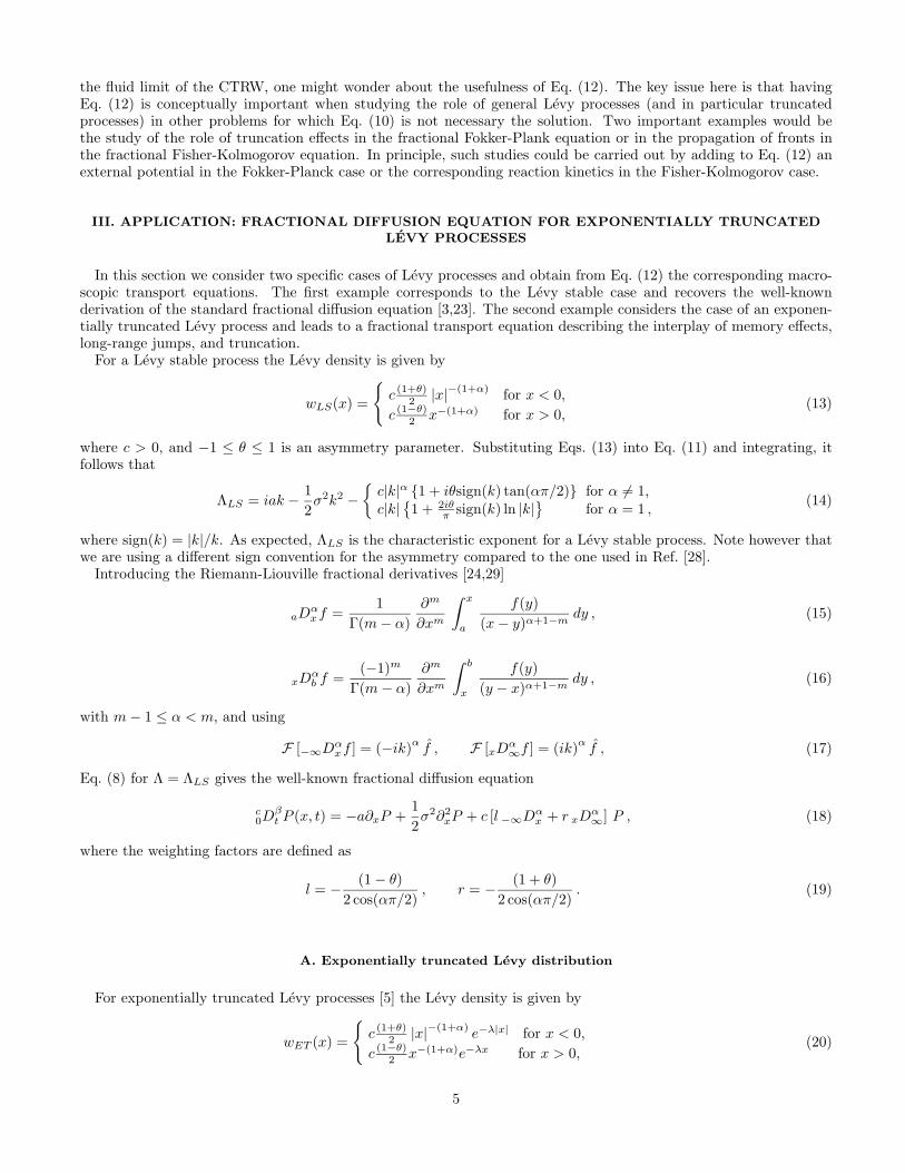
III. APPLICATION: FRACTIONAL DIFFUSION EQUATION FOR EXPONENTIALLY TRUNCATEDLEVY PROCESSES

In this section we consider two specific cases of Levy processes and obtain from Eq. (12) the corresponding macro-scopic transport equations. The first example corresponds to the Levy stable case and recovers the well-knownderivation of the standard fractional diffusion equation [3,23]. The second example considers the case of an exponen-tially truncated Levy process and leads to a fractional transport equation describing the interplay of memory effects,long-range jumps, and truncation.

For a Levy stable process the Levy density is given by

wLS(x) =

{c (1+θ)

2 |x|−(1+α) for x < 0,c (1−θ)

2 x−(1+α) for x > 0,(13)

where c > 0, and −1 ≤ θ ≤ 1 is an asymmetry parameter. Substituting Eqs. (13) into Eq. (11) and integrating, itfollows that

ΛLS = iak − 12σ2k2 −

{c|k|α {1 + iθsign(k) tan(απ/2)} for α �= 1,c|k|

{1 + 2iθ

π sign(k) ln |k|}

for α = 1 ,(14)

where sign(k) = |k|/k. As expected, ΛLS is the characteristic exponent for a Levy stable process. Note however thatwe are using a different sign convention for the asymmetry compared to the one used in Ref. [28].

Introducing the Riemann-Liouville fractional derivatives [24,29]

aDαx f =

1Γ(m − α)

∂m

∂xm

∫ x

a

f(y)(x − y)α+1−m

dy , (15)

xDαb f =

(−1)m

Γ(m − α)∂m

∂xm

∫ b

x

f(y)(y − x)α+1−m

dy , (16)

with m − 1 ≤ α < m, and using

F [−∞Dαx f ] = (−ik)α

f , F [xDα∞f ] = (ik)α

f , (17)

Eq. (8) for Λ = ΛLS gives the well-known fractional diffusion equation

c0D

βt P (x, t) = −a∂xP +

12σ2∂2

xP + c [l −∞Dαx + r xDα

∞] P , (18)

where the weighting factors are defined as

l = − (1 − θ)2 cos(απ/2)

, r = − (1 + θ)2 cos(απ/2)

. (19)

A. Exponentially truncated Levy distribution

For exponentially truncated Levy processes [5] the Levy density is given by

wET (x) =

{c (1+θ)

2 |x|−(1+α)e−λ|x| for x < 0,

c (1−θ)2 x−(1+α)e−λx for x > 0,

(20)

5

0 < α ≤ 2, c > 0, −1 ≤ θ ≤ 1 and λ ≥ 0. In this case the integral in Eq. (11) leads to the characteristic exponent [5]

ΛET = iak − σ2

2k2 − c

2 cos(απ/2)

{(1 + θ)(λ + ik)α + (1 − θ)(λ − ik)α − 2λα,(1 + θ)(λ + ik)α + (1 − θ)(λ − ik)α − 2λα − 2ikαθλα−1 ,

(21)

for 0 < α < 1 and 1 < α ≤ 2 respectively. The interpretation of the parameters is very similar as in the Levy stablecase. The damping parameter λ can be seen as the ‘strength’ of the exponential decay of the tails. When λ → 0,the further out in the tails of the distribution the dampening will take effect and the longer will the process take tobecome Gaussian as a consequence of the central limit theorem. Moreover, it is straightforward to observe that forλ > 0 the process will have finite moments of all orders. Substituting Eq. (21) into Eq. (8) and using

F[e−λx

−∞Dαx eλx P

]= (λ − ik)α

P , F[eλx

xDα∞ e−λx P

]= (λ + ik)α

P (22)

we obtain, after inverting the Fourier transform,

c0D

βt P = −V ∂xP +

σ2

2∂2

xP + cDα,λx P − νP , (23)

where the λ-truncated fractional derivative operator of order α, Dα,λx , is defined as

Dα,λx = le−λx

−∞Dαx eλx + reλx

xDα∞ e−λx , (24)

where V = a for 0 < α < 1, and V = a − v for 1 < α < 2 with

v =cαθλα−1

|cos (απ/2)| , (25)

and

ν = − cλα

cos (απ/2). (26)

As expected, for λ = 0 Eq. (23) reduces to Eq. (18).

B. Crossover and slow convergence to subdiffusive transport

As an application of Eq. (23) we consider the interplay between memory effects and truncation. In particular, weshow that for β �= 1, in the presence of a truncated Levy process, the probability of first return exhibits a transitionfrom superdiffusive dynamics to subdiffusive dynamics. We also show that this transition manifests as a crossoverfrom algebraic decaying tails to exponentially decaying tails in the probability distribution function.

For a = 0 and σ = 0, the characteristic exponent in Eq.(21) satisfies the scaling relation ΛET (μk;μλ) = μαΛET (k; λ).Using Eq. (10), this scaling implies the following scaling for the propagator G

G(x, μt;λ) = μ−β/αG(μ−β/αx, t;μβ/αλ

). (27)

Note that due to the dependence on λ there is no space-time self-similarity, physically the truncation introduces thepreferred length scale 1/λ that breaks the scale invariance. That is, the probability distribution function at a time μtcannot be obtained from a simple rescaling in x of the probability distribution function at t, unless λ is also rescaled.

To gain some intuition on the role of truncation consider the moments of the propagator

〈xn〉 =∫ ∞

−∞xnG(x, t)dx = (−i)n ∂nG(k, t)

∂kn

∣∣∣∣∣k=0

, (28)

where according to Eq. (10), G = Eβ

[tβΛET

]. For λ = 0, only the moments of order n < α exist, which as discussed

before, is one of the drawbacks of the Levy-Stable distributions from the applications point of view. On the otherhand, for λ �= 0, the function ΛET (k) is C∞ at k = 0, and all the moments of the distribution exist. The first ordermoment exhibits the usual scaling

6

〈x〉 =V

Γ(β + 1)tβ , (29)

where V = a − v for 0 < α < 1, and V = a for 1 < α < 2, with v defined in Eq. (25). Here the truncation plays norole in the scaling exponent. However, note that depending on the values of α and the asymmetry parameter θ, thetruncation can increase or decrease the drift velocity a. For the time evolution of the variance the second momentgives

σ2 =⟨[x − 〈x〉]2

⟩=

[2

Γ(2β + 1)− 1

Γ2(β + 1)

]V 2t2β +

2 χ

Γ(β + 1)tβ , (30)

where we have introduced the effective diffusivity

χ =σ2

2+

cα|α − 1|2| cos(απ/2)|λ2−α

. (31)

The truncation increases the Gaussian diffusivity σ2/2 by a term inversely proportional to λ and directly proportionalto c, the strength of the truncated Levy density in Eq. (20). Furthermore, in the limit λ → 0, χ → ∞, a resultconsistent with the divergence of the second moment in the absence of truncation.

Of particular interest is the scaling in time of the probability of first return, G(x = 0, t). From the scaling relationin Eq. (27) we have G(0, t;λ) = t−β/αG(0, 1; tβ/αλ). In the absence of truncation, λ = 0, this implies the expectedscaling G(0, t) ∼ t−β/α which in the case α = 2, β = 1, reduces to the well-known diffusive scaling G(0, t) ∼ t−1/2.The scaling G(0, t) ∼ t−β/α remains valid for λ �= 0 and small enough times because limt→0 G(0, 1; tβ/αλ) = G(0, 1; 0).The long-time behavior is less trivial and leads to a different scaling. The decay of the Mittag-Leffler function impliesthat in the limit t → ∞ the maximum contribution to the integral in Eq. (10) comes from the region around k ∼ 0.Therefore, using stationary phase arguments we can get the leading order asymptotic behavior by Taylor expandingthe argument of the Mittag-Leffler function around k = 0. Note however that some care must be taken since, contraryto the usual situation involving exponentials, Eβ decays algebraically for β �= 1. Restricting attention to the symmetriccase, θ = 0, with no drift a = 0, and substituting the small k expansion ΛET = −χk2 + . . . into Eq. (10) we get

limt→∞

G(0, t;λ) ∼ 1π

∫ ∞

0

Eβ

[−χtβk2

]dk =

[1

π√

χ

∫ ∞

0

Eβ

(−u2

)du

]t−β/2 . (32)

Thus, the truncation gives rise to a transition in the scaling of the return probability from ∼ t−β/α, for t � 1, to∼ t−β/2, for t � 1. In the case 2β/α > 1 this corresponds to a transition from superdiffusive scaling to subdiffusivescaling. This transition is clearly observed in Fig. 1 that shows the return probability as function of time over tenorders of magnitude obtained from the direct numerical evaluation of the integral in Eq. (10) with α = 1.25, β = 0.75and θ = 0. From the scaling of the probability distribution in Eq. (27) it follows that the time τc for the crossover tosubdiffusive dynamics scales as

τc ∼ c−1/β λ−α/β . (33)

As expected, in the Markovian case, β = 1, we recover the scaling for ultraslow Gaussian convergence reported inRef. [4,6].

For symmetric, θ = 0, processes with 1 < α < 2 and a = σ = 0, the propagator in Eq. (10) can be written as

(π/λ)G (λx, τ) =∫ ∞

0

cos (λxu) Eβ

[τβΦ(u)

]du , (34)

where

Φ(u) =(1 + u2

)α/2cos

[α tan−1(u)

]− 1 , (35)

and

τ = [−c/ cos(απ/2)]λα/βt . (36)

Figure 2 shows the temporal evolution of the propagator G as function of x obtained from the numerical evaluationof Eq. (34) for α = 1.25 and β = 0.75. Because of the truncation, the evolution is not self-similar. In particular, thesolution exhibits a transition in (log-normal scale) from a concave profile shape at short times to a convex shape at

7

long times. At the crossover time scale, τ ∼ 1, the distribution exhibits a linear profile indicating exponential decay.To ease the comparison at different times we have rescaled the spatial dimension by σβ = tβ/2, which corresponds tothe scaling of the variance in the subdiffusive limit. To maintain the normalization of the probability, the vertical axishas been rescaled by σβ . Panel (a) shows the propagator in the small τ limit. As expected, in this case G exhibits thecharacteristic form of the Green’s function of the fractional diffusion equation for β < 1 < α < 2. The superimposeddashed line shows the function G∞

α,β(z) = z−(1+α). It is observed that for λx/σ � 1, G → G∞α,β . This result is

expected from the fact that for small τ the truncation effects are negligible, and the tails of G exhibit the algebraicscaling x−(1+α) corresponding to the solution of the standard (λ = 0) fractional diffusion equation. Panels (b), (c)and (d) show the propagator G at later times. The superimposed dashed line in panel (d) is a plot of the functionG∞

2,β(z) = za1 exp (−za2) with a1 = (β − 1)/(2− β) and a2 = 2/(2− β), which is the asymptotic form of the solutionof the subdiffusive (α = 2, 0 < β < 1) fractional equation [3]. Consistent with the fact that for τ � 1 truncationeffects are dominant, it is observed that for λx/σ � 1, G → G∞

2,β .

IV. CONCLUSIONS

We considered the fluid limit of the continuum time random walk model for the most general jump probabilitydistribution function in the Levy-Khintchine representation. The resulting integro-differential equation gives theprobability distribution function in the long-time, small-k (large scale) limit. The time evolution is governed bya fractional time derivative and the spatial evolution corresponds to the generator for a general Levy density. Asexpected, for Levy stable densities we recover the usual fractional diffusion equation. However, one of the maindrawbacks of Levy stable distributions from the applications point of view is that, due to the algebraic decaying tails,they have divergent moments. In the past, to circumvent this problem, several authors have proposed the use oftruncated Levy densities that lead to finite moments. Of particular interest are exponentially truncated densities inwhich the algebraic decay of the tails is damped by an exponential factor. These distributions have found widespreadapplicability in many areas including plasma physics, fluid mechanics, and finance. However, despite their importance,little is known about the role of these distributions in CTRW with memory and in the corresponding fluid limit. Herewe addressed this issue and formulated a macroscopic transport equation in terms of truncated fractional derivatives.Because of the truncation, the dynamics ultimately converge to the Gaussian case for β = 1 and to the standardsubdiffusive case for β < 1. However, the key issue is that convergence can be extremely slow and for time scales ofinterest to applications the process can be considered non-Gaussian but not described by Levy stable distribution.The proposed truncated fractional diffusion equation describes this intermediate asymptotic regime which can not becaptured by the standard fractional diffusion equation based on Riemann-Liouville derivatives. As an application ofthe truncated fractional equation we studied the interplay between truncation and memory effects. It was shown thatthe return probability distribution function exhibits a transition from the Levy stable scaling G(0, t) ∼ t−β/α at shorttimes, to G(0, t) ∼ tβ/2 scaling at long times. For 2β/α > 1 this corresponds to a transition from superdiffusive tosubdiffusive dynamics. The crossover time to subdiffusive behavior scales as τ ∼ λ−α/β where 1/λ is the truncationlength scale. The asymptotic behavior of the propagator (Green’s function) of the truncated fractional diffusionequation exhibits a transition from algebraic decay (characteristic of superdiffusive processes) for λα/βt � 1 tostretched Gaussian decay (characteristic of subdiffusive processes) for λα/βt � 1.

Acknowledgments

Alvaro Cartea acknowledges financial support from the Nuffield Foundation. Diego del-Castillo-Negrete gratefullyacknowledges the hospitality of Birkbeck College of the University of London during the elaboration of this work, andthanks Dr. Raul Sanchez and Dr. Ivan Calvo for helpful comments. Also, Diego del-Castillo-Negrete acknowledgessupport from the Oak Ridge National Laboratory, managed by UT-Battelle, LLC, for the U.S. Department of Energyunder contract DE-AC05-00OR22725.

[1] E. W. Montroll, and G. H. Weiss, J. Math. Physics, 6, 167, (1965).[2] E. W. Montroll, and M. F. Shlesinger, in Nonequilibrium Phenomena II.From Stochastics to Hydrodynamics. Eds. J. L.

Lebowitz and E. W. Montroll. Elsevier Science Publishers BV, 1984.

8

[3] R. Metzler, and J. Klafter, Phys. Rep., 339, 1, (2000).[4] R. N. Mantegna, and H.E. Stanley, Phys. Rev. Lett., 73, 2946 (1994).[5] I. Koponen, Phys. Rev. E., 52, 1197 (1995).[6] M. F. Shlesinger, Phys. Rev. Lett., 74, 4959 (1995).[7] R. Jha, P. K. Kaw, D. R. Kulkami, J. C. Parikh, and the ADITYA Team, Phys. Plasmas 10, 699 (2003).[8] B. Dubrulle, and J.-Ph. Laval, Eur. Phys. J. B, 143-146 (1998).[9] R. Bruno, L. Sorriso-Valvo, V. Carbone and B. Bavassano, Europhys. Lett. 66 (1), pp. 146-152 (2004).

[10] Mantegna, R.N. and Stanley, H.E., Nature 376, pp 46-49 (1995).[11] R. Balescu, Phys. rev. E 51, 4807 (1995).[12] B. Ph. van Milligen, R. Sanchez, and B. A. Carreras, Phys. Plasmas 11 2272 (2004).[13] D. del-Castillo-Negrete, B. A. Carreras, and V. E. Lynch, Phys. Plasmas 11, 3854 (2004).[14] D. del-Castillo-Negrete, B. A. Carreras, and V. E. Lynch, Phys. Rev. Lett., 94, 065003 (2005).[15] D. del-Castillo-Negrete, Phys. Plasmas 13, 082308 (2006).[16] B. A. Carreras, V. E. Lynch, and G. M. Zaslavsky, Phys. Plasmas 8, 5096 (2001).[17] I. M. Sokolov, A. V. Chechkin, and J. Klafter, Physica A, 336 245-251 (2004).[18] Meerschaert, Benson, Scheffler, Baeumer, Phys. Rev. E 65, 041103 (2002).[19] Scheffler, Meerschaert, J. Appl. Probab. 41, 623 (2004).[20] Piryatinska, Saichev, Woyczynski, Physica A, 349 (2005).[21] V. M. Kenkre, E. W. Montroll, and M. F. Shlesinger, J. Stat. Phys. 9 (1), 45-50 (1973).[22] R. Hilfer and L. Anton, Phys. Rev. E 51, R848 (1995).[23] E. Scalas. R. Gorenflo, and F. Mainardi, Phys. Rev. E, 69, 011107, (2004).[24] I. Podlubny, Fractional Differential Equations (Academic Press, San Diego, 1999).[25] A. Saichev, and G. M. Zaslasvsky, Chaos, 7 (4) 753-764 (1997).[26] F. Mainardi, Y. Luchko and G. Pagnini. Fractional Calculus and Applied Analysis, 4, No 2, 153-192, (2001).[27] K. Sato, Levy Processes and Infinitely Divisible Distributions (Cambridge University Press, UK, 1999).[28] G. Samorodnitsky, and M. S. Taqqu, Stable non-Gaussian random processes (Chapman & Hall, New York, 1994).[29] S. G. Samko, A. A. Kilbas, and O. I. Marichev, Fractional Integrals and Derivatives, (Gordon and Breach Science Publishers,

Amsterdam, 1993).

9

FIGURE CAPTIONS

FIG. 1. (Color online) Probability of first return, G(0, t), for the truncated fractional diffusion equation Eq. (23)obtained from the numerical evaluation of the general solution in Eq. (10) for Λ = ΛET with θ = 0, α = 1.25and β = 0.75. The solid line denotes the value of G(0, t), the steeper dashed lines corresponds to thesuperdiffusive scaling, G(0, t) ∼ t−β/α, and the less steep dashed line corresponds to the subdiffusive scalingG(0, t) ∼ t−β/2. The scaling constant in the horizontal axis is A = [c/| cos(απ/2)|]1/β .

FIG. 2. (Color online) Time evolution of the solution of the truncated, λ �= 0, fractional diffusion Eq. (23) for adelta function initial condition and a = σ = θ = 0, α = 1.25, and β = 0.75. The dashed lines in panels (a)and (d) correspond to the asymptotic behavior of the solution of the standard, λ = 0, fractional diffusionequation for (α, β) = (1.25, 0.75) and (α, β) = (2, 0.75) respectively. To ease the comparison at successivetimes, the axes have been rescaled by the variance in the subdiffusive limit, σβ = τβ/2. A slow transitiondue to the truncation is observed from the superdiffusive concave algebraic decaying profile in panel (a) tothe subdiffusive convex profile in panel (d) with asymptotic stretched Gaussian decay. At the crossover timescale, τ ∼ 1, the profile shows asymptotically vanishing curvature characteristic of exponential decay.

10

10-5

100

105

10-2

10-1

100

101

102

103

104

Aλα/β t

(π/λ

) G

(0,t)

∼ t−β/α

∼ t−β/2

FIGURE 1

0 1 2 3 410

-3

10-2

10-1

100

101

0 1 2 3 4 510

-3

10-2

10-1

100

101

0 1 2 310

-3

10-2

10-1

100

101

0 0.5 1 1.5 2 2.510

-3

10-2

10-1

100

101

FIGURE 2

(a) (b)

(c) (d)

τ = 0.0005 τ = 0.05

τ = 1 τ = 500

λ x / σβ

λ x / σβ λ x / σβ

(π σ

/λ)

G

β

(π σ

/λ)

G

β

(π σ

/λ)

G

β

(π σ

/λ)

G

β

λ x / σβ