Fine regularity of Lévy processes and linear (multi)fractional stable motion

$: Fine regularity of Lévy processes and linear (multi)fractional stable motion$
Fine regularity of Lévy processes and linear(multi)fractional stable motion

Paul Balançae-mail: [email protected]

url: www.mas.ecp.fr/recherche/equipes/modelisation_probabiliste

École Centrale ParisLaboratoire MAS, ECP

Grande Voie des Vignes - 92295 Châtenay-Malabry, France

Abstract: We investigate the regularity of Lévy processes within the 2-microlocalanalysis framework. A local description of sample paths is obtained, refining the classicspectrum of singularities determined by Jaffard. As a consequence of this result andthe properties of the 2-microlocal frontier, we are able to completely characterizethe multifractal nature of the linear fractional stable motion (extension of fractionalBrownian motion to α-stable measures) in the case of continuous and unboundedsample paths as well. The regularity of its multifractional extension is also determined,thereby providing an example of a stochastic process with a non-homogeneous andrandom multifractal spectrum.

AMS 2000 subject classifications: 60G07, 60G17, 60G22, 60G44.Keywords and phrases: 2-microlocal analysis, Hölder regularity, Lévy processes,multifractal spectrum, linear fractional stable motion.

1. Introduction

The study of sample path continuity and Hölder regularity of stochastic processes is a veryactive field of research in probability theory. The existing literature provides a variety ofuniform results on local regularity, especially on the modulus of continuity, for rather generalclasses of random fields (see e.g. Marcus and Rosen [30], Adler and Taylor [2] on Gaussianprocesses and Xiao [45] for more recent developments).

On the other hand, the structure of pointwise regularity is often more complex, inparticular as it often happens to behave erratically as time passes. Such sample pathbehaviour was first put into light for Brownian motion by Orey and Taylor [33] and Perkins[34]. They respectively studied fast and slow points, which characterize logarithmic variationsof the pointwise modulus of continuity, and proved that the sets of times with a givenpointwise regularity have a particular fractal geometry. Khoshnevisan and Shi [25] recentlyextended the fast points study to fractional Brownian motion.

As exhibited by Jaffard [22], Lévy processes with a jump compound also display an inter-esting pointwise behaviour. Indeed, for this class of random fields, the pointwise exponentvaries randomly inside a closed interval as time passes. This seminal work has been enhancedand extended by Durand [18], Durand and Jaffard [19] and Barral et al. [10]. Particularly, thelatter proves that Markov processes have a range of admissible pointwise behaviours muchwider than Lévy processes. In the aforementioned works, multifractal analysis happens tobe the key concept for the study and the characterisation of local fluctuations of pointwise

1

arX

iv:1

302.

3140

v1 [

mat

h.PR

] 1

3 Fe

b 20

13

mailto:[email protected]

http://www.mas.ecp.fr/recherche/equipes/modelisation_probabiliste

Paul Balança/Fine regularity of Lévy processes and linear (multi)fractional stable motion 2

regularity. In order to be more specific, let us first recall the definition of the different notionspreviously outlined.

Definition 1. A function f : R → Rd belongs to Cαt , with t ∈ R and α > 0, if there existC > 0, ρ > 0 and a polynomial Pt of degree less than α such that

∀u ∈ B(t, ρ); ‖f(u)− Pt(u)‖ ≤ C|t− u|α.

The pointwise Hölder exponent of f at t is defined by αf,t = supα ≥ 0 : f ∈ Cαt , whereby convention sup∅ = 0.

Multifractal analysis is concerned with the study of the level sets of the pointwise expo-nent, usually called the iso-Hölder sets of f ,

Eh =t ∈ R : αf,t = h

for every h ∈ R+ ∪ +∞. (1.1)

To describe the geometry of the collection (Eh)h∈R+ , and thereby to determine the arrange-ment of the Hölder regularity, we are interested in the local spectrum of singularities of f .It is usually denoted df (h, V ) and defined by

df (h, V ) = dimH(Eh ∩ V ) for every h ∈ R+ ∪ +∞ and V ∈ O, (1.2)

where O denotes the collection of nonempty open sets of R and dimH the Hausdorffdimension (by convention dimH(∅) = −∞).

Although (Eh)h∈R+ are random sets, stochastic processes such as Lévy processes [22],Lévy processes in multifractal time [9] and fractional Brownian motion happen to havea deterministic multifractal spectrum. Furthermore, these random fields are also said tobe homogeneous as the Hausdorff dimension dX(h, V ) is independent of the set V for allh ∈ R+. When the pointwise exponent is constant along sample paths, the spectrum isdescribed as degenerate, i.e. its support is reduced to a single point (e.g. the Hurst exponentin the case of f.B.m.). Nevertheless, Barral et al. [10] and Durand [17] provided examples ofrespectively Markov jump processes and wavelet random series with non-homogeneous andrandom spectrum of singularities.

As stated in Equations (1.1) and (1.2), classic multifractal analysis deals with the studyof the variations of pointwise regularity. Unfortunately, it is known that common Hölderexponents (local and pointwise as well) do not give a complete picture of the local regularity(see e.g the deterministic Chirp function t 7→ |t|α sin

(|t|−β

)detailed in [20]). Furthermore,

they also lack of stability under the action of pseudo-differential operators.2-microlocal analysis is one natural way to overcome these issues and obtain a more

precise description of the local regularity. It has first been introduced by Bony [13] in thedeterministic frame to study properties of generalized solutions of PDE. More recently,Herbin and Lévy Véhel [20] and Balança and Herbin [7] developed a stochastic approachbased on this framework to investigate the finer regularity of stochastic processes such asGaussian processes, martingales and stochastic integrals. In order to the study sample pathproperties in this frame, we need to recall the concept of 2-microlocal space.

Definition 2. Let t ∈ R, s′ ≤ 0 and σ ∈ (0, 1) such that σ−s′ /∈ N. A function f : R → Rd

belongs to the 2-microlocal space Cσ,s′

t if there exist C > 0, ρ > 0 and a polynomial Pt suchthat ∥∥(f(u)− Pt(u)

)−((f(v)− Pt(v)

)∥∥ ≤ C|u− v|σ(|u− t|+ |v − t|)−s′ , (1.3)


for all u, v ∈ B(t, ρ).The time-domain characterisation (1.3) of 2-microlocal spaces has been obtained by Seuret

and Lévy Véhel [41]. The original definition given by Bony [13] relies on the Littlewood-Paleydecomposition of tempered distributions, and thereby corresponds to a description in theFourier space. Another characterisation based on wavelet expansion has also been exhibitedby Jaffard [21]. The extension of Definition 2 to σ /∈ (0, 1) relies on the following importantproperty satisfied by 2-microlocal spaces (see Theorem 1.1 in [23]),

∀α > 0; f ∈ Cσ,s′

t ⇐⇒ Iαf ∈ Cσ+α,s′t , (1.4)

where Iαf designates the fractional integral of f of order α. As a consequence of (1.4), theapplication of Equation (1.3) to iterated integrals or differentials of f provides an extensionof Definition 2 to any σ ∈ R \ Z, which is sufficient for the purpose of this paper.

Similarly to the pointwise Hölder exponent, the introduction of 2-microlocal spaces leadsnaturaly to the definition of regularity tool named the 2-microlocal frontier and given by

∀s′ ∈ R; σf,t(s′) = supσ ∈ R : f ∈ Cσ,s

′

t

.

2-microlocal spaces enjoy several inclusion properties which imply that the map s′ 7→ σf,t(s′)is well-defined and display the following features:• σf,t(·) is a concave non-decreasing function;• σf,t(·) has left and right derivatives between 0 and 1.

As a function, the 2-microlocal frontier σf,t(·) offers a more complete description of the localregularity. In particular, it embraces the local Hölder exponent since αf,t = σf,t(0). Further-more, as stated in [32], if the modulus of continuity of f satisfies ω(h) = O (1/|log(h)|), thepointwise exponent can also be retrieved using the formula αf,t = − infs′ : σf,t(s′) ≥ 0.Note that the previous formula can not directly deduced from Equation 1.3 since Definition2 does not stand when σ = 0. [32] provides an example of generalized function which doesnot satisfy this relation.

As observed [20], Brownian motion provides a simple instance of 2-microlocal frontier inthe stochastic frame: almost surely for all t ∈ R, σB,t satisfies

∀s′ ∈ R; σB,t(s′) =(1

2 + s′)∧ 1

2 , (1.5)

In this paper, the 2-microlocal approach is combined with the classic use of multifractalanalysis to obtain a finer description of the regularity of stochastic processes. Following thepath of [22, 18, 19], we refine the multifractal description of Lévy processes (Section 2) andobserve in particular that the use of the 2-microlocal formalism allows to capture subtlebehaviours that can not be characterized by the classic spectrum of singularities.

This finer analysis of sample path properties of Lévy processes happens to be very usefulfor the study of another class of processes named linear fractional stable motion (LFSM).The LFSM is a common α-stable self-similar process with stationary increments, and can beseen as an extension of the fractional Brownian motion to the non-Gaussian frame. Since italso has long range dependence and heavy tails, it is of great interest in modelling. In Section3, we completely characterize the multifractal nature of the LFSM, and thereby illustratethe fact that 2-microlocal analysis is well-suited to study the regularity of unbounded samplepaths as well as continuous ones.


1.1. Statement of the main results

As it is well known, an Rd-valued Lévy process (Xt)t∈R+ has stationary and independentincrements. Its law is determined by the Lévy-Khintchine formula (see e.g. [40]): for allt ∈ R+ and λ ∈ Rd, E[ei〈λ,Xt〉] = etψ(λ) where ψ is given by

∀λ ∈ Rd; ψ(λ) = i〈a, λ〉 − 12 〈λ,Qλ〉+

∫Rd

(ei〈λ,x〉 − 1− i〈λ, x〉1‖x‖≤1

)π(dx).

Q is a non-negative symmetric matrix and π a Lévy measure, i.e. a positive Radon measureon Rd \ 0 such that

∫Rd(1 ∧ ‖x‖2)π(dx) <∞.

Throughout this paper, it will always be assumed that π(Rd) = +∞. Otherwise, theLévy process simply corresponds to the sum of a compound Poisson process with drift anda Brownian motion whose regularity can be simply deduced.

Sample path properties of Lévy processes are known to depend on the growth of the Lévymeasure near the origin. More precisely, Blumenthal and Getoor [12] defined the followingexponents β and β′,

β = infδ ≥ 0 :

∫Rd

(1 ∧ ‖x‖δ

)π(dx) <∞

and β′ =

β if Q = 0;2 if Q 6= 0.

(1.6)

Owing to π’s definition, β, β′ ∈ [0, 2]. Pruitt [36] proved that αX,0a.s.= 1/β when Q = 0. Note

that several other exponents have been defined in the literature focusing on Lévy processessample paths properties (see e.g. [26, 27] for some recent developments).

Jaffard [22] studied the spectrum of singularities of Lévy processes under the followingassumption on the measure π,∑

j∈N

2−j√Cj log(1 + Cj) <∞, where Cj =

∫2−j−1<‖x‖≤2−j

π(dx). (1.7)

Under the Hypothesis (1.7), Theorem 1 in [22] states that the multifractal spectrum of aLévy process X is almost surely equal to

∀V ∈ O; dX(h, V ) =

βh if h ∈ [0, 1/β′);1 if h = 1/β′;−∞ if h ∈ (1/β′,+∞].

(1.8)

Note that Equation (1.8) still holds when β = 0. Durand [18] extended this result toHausdorff g-measures, where g is a gauge function, and Durand and Jaffard [19] generalizedthe study to multivariate Lévy fields.

We establish in Proposition 1 a new proof of the multifractal spectrum (1.8) which doesnot require Assumption (1.7). We observe that results obtained in [18] on Hausdorff g-measure are also extended using this method.

In order to refine the spectrum of singularities (1.8), we focus on the study of the2-microlocal frontier of Lévy processes. For that purpose, we introduce and study thecollections of sets (Eh)h∈R+ and (Eh)h∈R+ respectively defined by

Eh =t ∈ Eh : ∀s′ ∈ R; σX,t(s′) = (h+ s′) ∧ 0

and Eh = Eh \ Eh.


The family (Eh)h∈R+ represents the set of times at which the 2-microlocal behaviour is rathercommon (and thus similar the 2-microlocal frontier (1.5) of Brownian motion), whereasat points which belong (Eh)h∈R+ , the 2-microlocal frontier has an unusual form, with inparticular a slope different from 1 at s′ = −h.

The next statement gathers our main result on the 2-microlocal regularity of Lévy pro-cesses.

Theorem 1. Sample paths of a Lévy process X almost surely satisfy

∀V ∈ O; dimH(Eh ∩ V ) =

βh if h ∈ [0, 1/β′);1 if h = 1/β′;−∞ if h ∈ (1/β′,+∞].

(1.9)

The collection of sets (Eh)h∈R+ enjoys almost surely

∀V ∈ O; dimH(Eh ∩ V ) ≤

2βh− 1 if h ∈ (1/2β, 1/β′);−∞ if h ∈ [0, 1/2β] ∪ [1/β′,+∞].

(1.10)

Furthermore, the 2-microlocal frontier at t ∈ Eh satisfies σX,t(s′) ≤(h+s′2βh

)∧( 1β′ + s′

)∧ 0

for all s′ ≥ −1/β′ − 1.

Remark 1. The previous statement induces that dimH(Eh) < dimH(Eh) for all h ∈[0, 1/β′]. Hence, from a Hausdorff dimension point of view, the majority of the times t ∈ R+have a rather classic 2-microlocal frontier s′ 7→ (αX,t + s′) ∧ 0.

Remark 2. The collection of sets (Eh)h∈R+ illustrates the fact that 2-microlocal analysiscan capture particular behaviours that are not necessarily described by a classic multifractalspectrum.

Examples 1 and 2 constructed in Section 2.3 show that different behaviours may occur,depending on properties of the Lévy measure. The first one provides a class of Lévy processeswhich satisfy Eh = ∅ for all h ∈ [0, 1/β′]. On the other hand, in Example 2 is constructeda collection of Lévy measures (πh)h∈(1/2β′,1/β′) such that the related Lévy process almostsurely enjoys Eh 6= ∅.

It remains an open question to completely characterize the collection (Eh)h∈R+ in termsof the Lévy measure π (Examples 1 and 2 indeed prove that the Blumenthal-Getoor exponentβ is not sufficient).

Remark 3. Although sample paths of Lévy processes do not satisfy the condition ω(h) =O(1/|log(h)|) outlined in the introduction, Theorem 1 nevertheless ensures that the pointwiseHölder exponent can be retrieved from the 2-microlocal frontier at any t ∈ R+ using theformula αX,t = − infs′ : σX,t(s′) ≥ 0.

Since this work extends the study of the classic spectrum of singularities, it is also quitenatural to investigate geometrical properties of the sets (Eσ,s′)σ,s′∈R defined by

Eσ,s′ =t ∈ R+ : ∀u′ > s′; X• ∈ Cσ,u

′

t and ∀u′ < s′; X• /∈ Cσ,u′

t

.

Theorem 1 induces the next statement.


Corollary 1. A Lévy process X satisfies almost surely for any σ ∈ [−1, 0],

∀V ∈ O; dimH(Eσ,s′ ∩ V ) =

βs if s ∈ [0, 1/β′);1 if s = 1/β′;−∞ otherwise.

(1.11)

where s denotes the common 2-microlocal parameter s = σ−s′. Furthermore, for all s′ ∈ R,E0,s′ = E−s′ and Eσ,s′ is empty if σ > 0.

Corollary 1 generalizes the multifractal formula (1.8) since the spectrum of singularitiescorresponds to the case σ = 0. Note that the subtle behaviour exhibited in Theorem 1 is notcaptured by Equality (1.11). As outlined in the proof (Section 2.2), this property disappearsbecause the sets (Eh)h are negligible compared to (Eh)h in terms of Hausdorff dimension.

Regularity results established in Theorem 1 also happen to be interesting outside the scopeof Lévy processes, thanks to the powerful properties satisfied the 2-microlocal frontier. Moreprecisely, it allows to characterized the multifractal nature of the linear fractional stablemotion (LFSM). This process is usually defined by the following stochastic integral (see e.g.[39])

Xt =∫

R

(t− u)H−1/α

+ − (−u)H−1/α+

Mα,β(du), (1.12)

where Mα,β is an α-stable random measure and H ∈ (0, 1). Several regularity propertieshave been determined in the literature. In particular, sample paths are known to be nowherebounded [29] if H < 1/α, whereas they are Hölder continuous when H > 1/α. In this lattercase, Takashima [44], Kôno and Maejima [28] proved that the pointwise and local Hölderexponents satisfy almost surely H − 1/α ≤ αX,t ≤ H and αX,t = H − 1/α. In the sequel,we will assume that α ∈ [1, 2), which is in particular required to obtain Hölder continuoussample paths (H > 1/α).

Using an alternative representation of LFSM obtained in Proposition 2, we enhance theaforementioned regularity results and obtain a description of the multifractal spectrum ofthe LFSM.Theorem 2. Let X be a linear fractional stable motion parametrized by α ∈ [1, 2) andH ∈ (0, 1). It satisfies almost surely for all σ ∈

[H − 1

α − 1, H − 1α

],

∀V ∈ O; dimH(Eσ,s′ ∩ V ) =α(s−H) + 1 if s ∈

[H − 1

α , H];

−∞ otherwise.(1.13)

where s = σ − s′. Furthermore, for all s′ ∈ R, Eσ,s′ is empty if σ > H − 1α .

Remark 4. In the continuous case H > 1/α, Theorem 2 ensures that the multifractalspectrum (σ = 0) of the LFSM is equal to

∀V ∈ O; dX(h, V ) =α(h−H) + 1 if h ∈

[H − 1

α , H];


Spectrum 1.14 and Equation (1.13) clearly extend the aforementioned lower and upperbounds obtained on the pointwise and local Hölder exponents. We also note that as it couldbe expected, the LFSM is an homogeneous multifractal process.


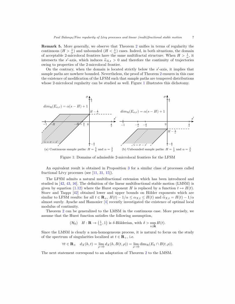
Remark 5. More generally, we observe that Theorem 2 unifies in terms of regularity thecontinuous (H > 1

α ) and unbounded (H < 1α ) cases. Indeed, in both situations, the domain

of acceptable 2-microlocal frontiers have the same multifractal structure. When H > 1α , it

intersects the s′-axis, which induces αX,t > 0 and therefore the continuity of trajectoriesowing to properties of the 2-microlocal frontier.

On the contrary, when the domain is located strictly below the s′-axis, it implies thatsample paths are nowhere bounded. Nevertheless, the proof of Theorem 2 ensures in this casethe existence of modification of the LFSM such that sample paths are tempered distributionswhose 2-microlocal regularity can be studied as well. Figure 1 illustrates this dichotomy.

s′

σ

0−1

−1

2

dimH(Eσ,s′) = α(s−H) + 1

1

2

1

2

−H + 1

α

H −1

α

−H

s = σ − s′

(a) Continuous sample paths: H = 56 and α = 3

2

s′

σ

0−1

−1

2

dimH(Eσ,s′) = α(s−H) + 1

1

2

1

2

H −1

α

−1

2−

1

α

s = σ − s′

(b) Unbounded sample paths: H = 12 and α = 3

2

Figure 1: Domains of admissible 2-microlocal frontiers for the LFSM

An equivalent result is obtained in Proposition 3 for a similar class of processes calledfractional Lévy processes (see [11, 31, 15]).

The LFSM admits a natural multifractional extension which has been introduced andstudied in [42, 43, 16]. The definition of the linear multifractional stable motion (LMSM) isgiven by equation (1.12) where the Hurst exponent H is replaced by a function t 7→ H(t).Stoev and Taqqu [42] obtained lower and upper bounds on Hölder exponents which aresimilar to LFSM results: for all t ∈ R+, H(t)− 1/α ≤ αX,t ≤ H(t) and αX,t = H(t)− 1/αalmost surely. Ayache and Hamonier [4] recently investigated the existence of optimal localmodulus of continuity.

Theorem 2 can be generalized to the LMSM in the continuous case. More precisely, weassume that the Hurst function satisfies the following assumption,

(H0) H : R →( 1α , 1

)is δ-Hölderian, with δ > sup

t∈RH(t).

Since the LMSM is clearly a non-homogeneous process, it is natural to focus on the studyof the spectrum of singularities localized at t ∈ R+, i.e.

∀t ∈ R+ dX(h, t) = limρ→0

dX(h,B(t, ρ)) = limρ→0

dimH(Eh ∩B(t, ρ)).

The next statement correspond to an adaptation of Theorem 2 to the LMSM.


Theorem 3. Let X be a linear multifractional stable motion parametrized by α ∈ (1, 2)and an (H0)-Hurst function H. It satisfies almost surely for all t ∈ R and for all σ ∈[H(t)− 1

α − 1, H(t)− 1α

),

limρ→0

dimH(Eσ,s′ ∩B(t, ρ)

)=α(s−H(t)

)+ 1 if s ∈

[H(t)− 1

α , H(t)];


where s = σ − s′. Furthermore, the set Eσ,s′ ∩ B(t, ρ) is empty for any σ > H(t) − 1α and

ρ > 0 sufficiently small.

Remark 6. Theorem 3 extends results presented in [42, 43]. In particular, it ensures thatthe localized multifractal spectrum is equal to

∀t ∈ R+; dX(h, t) =α(h−H(t)

)+ 1 if h ∈

[H(t)− 1

α , H(t)];


Moreover, we observe that Proposition 2 and Theorem 3 still hold when the Hurst functionH(·) is a continuous random process. Thereby, similarly to the works of Barral et al. [10]and Durand [17], it provides a class stochastic processes whose spectrum of singularities,given by equation (1.16), is non-homogeneous and random.

2. Regularity of Lévy processes

In this section, X will designate a Lévy process parametrized by the generating triplet(a,Q, π). Lévy-Ito decomposition states that it can represented as the sum of three indepen-dent processes B, N and Y , where B is a d-dimensional Brownian motion, N is a compoundPoisson process with drift and Y is a Lévy process characterized by

(0, 0, π(dx)1‖x‖≤1

).

Without any loss of generality, we restrict the study to the time interval [0, 1]. As noticedin [22], the componentN does not affect the regularity ofX since its trajectories are piecewiselinear with a finite number of jumps. Sample path properties of Brownian motion are well-known and therefore, we first focus in the sequel on the study of the jump process Y .

We know there exists a Poisson measure J(dt, dx) of intensity L1⊗π such that Y is givenby

Yt = limε→0

[∫[0,t]×D(ε,1)

xJ(ds,dx)− t∫D(ε,1)

xπ(dx)],

where for all 0 ≤ a < b, D(a, b) = x ∈ Rd : a < ‖x‖ ≤ b. Moreover, as presented in [40](Theorem 19.2), the convergence is almost surely uniform on any bounded interval. For anym ∈ R+, Y m will denote the following Lévy process

Y mt = limε→0

[∫[0,t]×D(ε,2−m)

xJ(ds,dx)− t∫D(ε,2−m)

xπ(dx)]. (2.1)

2.1. Pointwise exponent

We extend in this section the multifractal spectrum (1.8) to any Lévy process. To beginwith, we prove two technical lemmas that will be extensively used in the sequel.


Lemma 2.1. For any δ > β, there exists a constant Cδ > 0 such that for all m ∈ R+

P(

supt≤2−m

∥∥Y m/δt

∥∥1 ≥ m2−m/δ

)≤ Cδe−m.

Proof. Let δ > β. We first observe that for any m ∈ R+,supt≤2−m

∥∥Y m/δt

∥∥1 ≥ m2−m/δ

=

⋃ε∈−1,1d

supt≤2−m

⟨ε, Y

m/δt

⟩≥ m2−m/δ

Therefore, it is sufficient to prove that there exists Cδ > 0 such that for any ε ∈ −1, 1d,

P(

supt≤2−m

⟨ε, Y

m/δt

⟩≥ m2−m/δ

)≤ Cδe−m.

Let λ = 2m/δ and Mt = eλ〈ε,Ym/δt 〉 for all t ∈ R+. According to Theorem 25.17 in [40], we

have E[Mt] = expt∫D(0,2−m/δ)

(eλ〈ε,x〉 − 1− λ〈ε, x〉

)π(dx)

. Furthermore, we observe that

for all s ≤ t ∈ R+,

E[Mt | Fs ] = Ms exp

(t− s)∫D(0,2−m/δ)

(eλ〈ε,x〉 − 1− λ〈ε, x〉

)π(dx)

≥Ms,

since for any y ∈ R, ey− 1− y ≥ 0. Hence, M is a positive submartingale, and using Doob’sinequality (Theorem 1.7 in [37]), we obtain

P(

supt≤2−m

⟨ε, Y

m/δt

⟩≥ m2−m/δ

)= P

(supt≤2−m

Mt ≥ em)≤ e−mE[M2−m ].

For all y ∈ [−1, 1], we note that ey − 1− y ≤ y2. Thus, for any m ∈ R+,

E[M2−m ] ≤ exp

2−m∫D(0,2−m/δ)

λ2〈ε, x〉2π(dx)≤ exp

2−m

∫D(0,2−m/δ)

λ2‖x‖2π(dx).

If β < 2, let γ > 0 be such that β < γ < 2 and γ < δ. Then, we obtain

2−m∫D(0,2−m/δ)

λ2‖x‖2π(dx) = 2−m(1−2/δ)∫D(0,2−m/δ)

‖x‖γ · ‖x‖2−γπ(dx)

≤ 2−m(1−2/δ)2−m/δ(2−γ)∫D(0,1)

‖x‖γπ(dx)

= 2−m(1−γ/δ)∫D(0,1)

‖x‖γπ(dx) ≤∫D(0,1)

‖x‖γπ(dx),

since γ < δ. If β = 2, we simply observe that

2−m∫D(0,2−m/δ)

λ2‖x‖2π(dx) ≤ 2−m(1−2/δ)∫D(0,1)

‖x‖2π(dx) ≤∫D(0,1)

‖x‖2π(dx),

as δ > 2. Therefore, there exists Cδ > 0 such that for all m ∈ R+, E[M2−m ] ≤ Cδ, whichproves the lemma.


Lemma 2.2. For any δ > β, there exists a constant Cδ > 0 such that for all m ∈ R+

P(

supu,v∈[0,1],|u−v|≤2−m

∥∥Y m/δu − Y m/δv

∥∥1 ≥ 3m2−m/δ

)≤ Cδe−Dm,

where D is positive constant independent of δ.

Proof. We note that for any m ∈ R+ and all δ > β,sup

u,v∈[0,1],|u−v|≤2−m


∥∥1 ≥ 3m2−m/δ

⊆2m−1⋃k=0

supt≤2−m

∥∥Y m/δt+k2−m − Ym/δk2−m

∥∥1 ≥ m2−m/δ

.

Therefore, the stationarity of Lévy processes and Lemma 2.1 yield

P(

supu,v∈[0,1],|u−v|≤2−m


∥∥1 ≥ 3m2−m/δ

)≤ 2mCδe−m = Cδe

−Dm,

where D = 1− log(2).

Let us recall the definition of the collection of random sets (Aδ)δ>0 introduced in [22].For every ω ∈ Ω, S(ω) denotes the countable set of jumps of Y•(ω). Moreover, for any ε > 0,let Aεδ be

Aεδ =⋃

t∈S(ω)‖∆Yt‖≤ε

[t− ‖∆Yt‖δ, t+ ‖∆Yt‖δ

].

Then, the random set Aδ is defined by Aδ = lim supε→0+ Aεδ. As noticed in [22], if t ∈ Aδ,we necessarily have αY,t ≤ 1

δ . The other side inequality is obtained in the next statement,extending the proof of Proposition 2 from [22].

Proposition 1. Let δ > β. Almost surely for all t ∈ [0, 1] \ S(ω), Y satisfies

t /∈ Aδ =⇒ αY,t ≥ 1δ .

Proof. Using Lemma 2.2 and Borel-Cantelli lemma, we know that almost surely, there existsM(ω) such that for any m ∈ N ≥M(ω),

∀u, v ∈ [0, 1] such that |u− v| ≤ 2−m;∥∥Y m/δv − Y m/δu

∥∥ ≤ Cm2−m/δ, (2.2)

where C is a positive constant. Furthermore, as t /∈ Aδ, there exists ε0 > 0 such that for allε ≤ ε0, t /∈ Aεδ. Then, for all u in the neighbourhood of t, we have∫

[t,u]×D(ε0,1)xJ(ds,dx)− (t− u)

∫D(ε0,1)

xπ(dx) = −(t− u)∫D(ε0,1)

xπ(dx),

Since a linear component does not contribute to the pointwise exponent, we only have toconsider the remaining part of the Lévy process to characterize the regularity.


Let u ∈ [0, 1] and m ∈ N such that 2−m−1 ≤ |t − u| < 2−m. m can be supposed largeenough to satisfy m ≥ M(ω). Let ε1 = 2−m/δ. For any jump ∆Ys whose norm is in theinterval [ε1, ε0], we have ‖∆Ys‖δ ≥ εδ1 > |t− u|.

Therefore, there is no such jumps ∆Ys in the interval [t, u] and∫

[t,u]×D(ε1,ε0) xJ(ds,dx) =0. Let now distinguish two different cases.

1. If δ ≥ 1, we obtain∥∥∥(t− u)∫D(ε1,ε0)

xπ(dx)∥∥∥ ≤ |t− u|∫

D(ε1,ε0)‖x‖δ · ‖x‖1−δ π(dx)

≤ |t− u| · ε1−δ1

∫D(ε1,ε0)

‖x‖δ π(dx) ≤ C|t− u|1/δ.

Furthermore,∥∥Y m/δt − Y m/δu

∥∥ ≤ C log(|t − u|) · |t − u|1/δ according to equation (2.2).Hence, these two inequalities imply αY,t ≥ 1

δ .2. If δ < 1 (and thus β < 1), we have (t−u)

∫D(ε1,ε0) xπ(dx) = (t−u)

∫D(0,ε0) xπ(dx)−(t−

u)∫D(0,ε1) xπ(dx). The component (t−u)

∫D(0,ε0) xπ(dx) is linear in the neighbourhood

of t, and therefore can be ignored. For the second integral, we similarly observe that∥∥∥(t− u)∫D(0,ε1)

xπ(dx)∥∥∥ ≤ |t− u| · ε1−δ

1

∫D(0,ε1)

‖x‖δ π(dx) ≤ C|t− u|1/δ.

This last inequality and Equation (2.2) prove that αY,t ≥ 1δ .

Proposition 1 ensures that almost surely

∀h > 0; Eh =( ⋂δ<1/h

Aδ

)\( ⋃δ>1/h

Aδ

)\ S and E0 =

(⋂δ>0

Aδ

)∪ S. (2.3)

Furthermore, since the estimate of the Hausdorff dimension obtained in [22] does not relyon Assumption (1.7), Y satisfies almost surely

∀V ∈ O; dimH(Eh ∩ V ) =βh if h ∈ [0, 1/β];−∞ else.

2.2. 2-microlocal frontier: proof of Theorem 1

Let us now study the 2-microlocal frontier of Lévy processes. According to Theorem 3.13 in[32], for all t ∈ [0, 1] and any s′ > −αY,t, the sample path Y•(ω) almost surely belongs to the2-microlocal space C0,s′

t . Furthermore, owing to the density of the set of jumps S(ω) in [0, 1],we necessarily have Y•(ω) /∈ Cσ,s

′

t for any σ > 0 and s′ ∈ R. Hence, since the 2-microlocalfrontier is a concave function with left- and right-derivatives between 0 and 1, we obtainthat almost surely, for all t ∈ [0, 1]

∀s′ ∈ R+; σY,t(s′) ≥ (αY,t + s′) ∧ 0 and σY,t(s′) ≤ 0.


Therefore, we consider in the sequel on the negative component of the 2-microlocal frontierof Y . As outlined in the introduction and according to Definition 2 of 2-microlocal spaces,we need to study the increments around t of the integral of the process Y , i.e.

∀u, v ∈ B(t, ρ);∥∥∥∥∫ v

b

Ys ds− Pt(v)−∫ u

b

Ys ds+ Pt(u)∥∥∥∥, (2.4)

where b < t is fixed. The form of the polynomial Pt depends on β. If β ≥ 1, we only need toremove a linear component equal to

∫ ubYt ds, and therefore the increment simply corresponds

to∫ vu

(Ys − Yt) ds. On the other hand, if β < 1, the proof of Proposition 1 induces that wealso need to subtract the compensation term s 7→ (s− t)

∫D(0,1) xπ(dx). Then, in this case,

we have to study

∀u, v ∈ B(t, ρ);∥∥∥∥∫ v

u

Ys − Yt − (s− t)

∫D(0,1)

xπ(dx)

ds∥∥∥∥.

For sake of readability, we divide the proof of Theorem 1 and its corollary in differenttechnical lemmas. We begin by obtaining a global upper bound of the frontier.

Lemma 2.3. Almost surely for all t ∈ [0, 1], the 2-microlocal frontier σY,t satisfies

∀s′ ∈ R s.t σY,t(s′) ∈ [−1, 0]; σY,t(s′) ≤( 1β

+ s′)∧ 0. (2.5)

Proof. Let m ∈ N, ε > 0, α = β(1 − 2ε) and γ = β(1 + 4ε). As stated in [22], to provethat αY,t ≤ 1/β, it is sufficient to exhibit for any ε > 0 a sequence (tn)n∈N such that‖∆Ytn‖ = 2−n and |t − tn| ≤ 2−nα. In order to extend this inequality to the 2-microlocalfrontier and obtain equation (2.5), we need to reinforce the previous statement and showthat in the neighbourhood of tn, there is no other jump of similar size.

More precisely, let consider d2mαe consecutive intervals Ij of size 2−mα. The family (Ij)jforms a cover of [0, 1]. Each Ij can be divided into at least b2m(γ−α)c disjoint of intervalsIi,j of size 2−mγ . Finally, let Ii,j = I1

i,j ∪ I2i,j ∪ I3

i,j be the three consecutive intervals of samesize inside Ii,j . We investigate the probability of the following event

Ai,j =J(I1

i,j , D(2−m, 1)) = 0∩J(I3

i,j , D(2−m, 1)) = 0∩

J(I2i,j , D(2−m, 1)) = 1

∩J(Ii,j , D(2−m(1+ε), 2−m)) = 0

,

Since J is a Poisson measure, Ai,j corresponds to the intersection of independent events andwe have

P(Ai,j) = 2−mγ

3 π(D(2−m, 1)) · exp(−2−mγπ(D(2−m, 1)) + 2−mγπ(D(2−m(1+ε), 2−m))

).

As described in [12], β can also be defined by β = infδ ≥ 0 : lim supr→0 r

δπ(B(r, 1)

)<∞

.

Therefore, there exists r0 > 0 such that for all r ∈ (0, r0], π(B(r, 1)

)≤ r−β(1+ε). Then, for

all m ∈ N large enough, we obtain

P(Ai,j) ≥ 2−mγ−2π(D(2−m, 1)) · exp(−2 · 2−mβε

)= 2−mγ−2π(D(2−m, 1)) · (1 + om(1)).


According to the definition of β, there also exists an increasing sequence (mn)n∈N suchthat for all n ∈ N, π(D(2−mn , 1)) ≥ 2mnβ(1−ε). Therefore, along this sub-sequence, we haveP(Ai,j) ≥ 2−5mnβε−2 · (1 + on(1)) for any n ∈ N.

Let now consider the event Bn,j defined by

Bn,j =b2mn(γ−α)c⋂

i=1Aci,j .

Since the events (Ai,j)i are identical and independent, we obtain

P(Bn,j) = P(Ac1,j)b2mn(γ−α)c ≤

(1− 2−5mnβε−2 · (1 + o(1))

)2mn(γ−α)−1,

which leads to log(P(Bn,j)

)≤ 2mn(γ−α)−1 log

(1− 2−5mnβε−2 · (1 + o(1))

)= −2mnβε−3 · (1 +

o(1)), since γ − α = 6βε. Therefore, for all n ∈ N, P(Bn,j) ≤ exp(−2mnβε−3 · (1 + o(1))

).

Finally, let Bn = ∪d2mnαe

j=1 Bn,j . For all n ∈ N, it satisfies

P(Bn) ≤ 2mnα+1 · exp(−2mnβε−2 · (1 + o(1))

)≤ exp

(Cmn − 2mnβε−2 · (1 + o(1))

),

where C is a positive constant. Hence, using Borel-Cantelli lemma, there exists an event Ω0of probability 1 such that for any ω ∈ Ω0, there exists N(ω) and for all n ≥ N(ω),

ω ∈ Bcn(ω) =d2mnαe⋂j=1

b2mn(γ−α)c⋃i=1

Ai,j .

Let now t ∈ [0, 1], ω ∈ Ω0 and n ≥ N(ω). There exist i, j ∈ N such that t ∈ Ij and ω ∈ Ai,j .Hence, according to the definition of the event Ai,j , there is tn ∈ Ii,j such that ‖∆Ytn‖ ≥2−mn and |t − tn| ≤ 2−mnα. Furthermore, there is no other jump of size greater than2−mn(1+ε) in the ball B(tn, ρn), where ρn = 2−mnγ/3. Since ∆Ytn = (Ytn−Yt)+(Yt−Ytn−),we necessarily have ‖Ytn − Yt‖ ≥ 2−mn−1 or ‖Yt − Ytn−‖ ≥ 2−mn−1. Without any loss ofgenerality, we assume in the sequel that ‖Ytn − Yt‖ ≥ 2−mn−1 is satisfied.

As previously outlined, we need to study the increments described in equation (2.4).Specifically, we observe on the interval [tn, tn + ρn] that∥∥∥∥∫ tn+ρn

tn

(Ys − Yt) ds∥∥∥∥ =

∥∥∥∥ρn · (Ytn − Yt) +∫ tn+ρn

tn

(Ys − Ytn) ds∥∥∥∥

≥ ρn ·∥∥Ytn − Yt∥∥− ∫ tn+ρn

tn

∥∥Ys − Ytn∥∥ds.

Let obtain an upper bound for the second term. There is no jump of size greater than2−mn(1+ε) in the interval (tn, tn+ρn]. Therefore, for all s ∈ (tn, tn+ρn], we have Ys−Ytn =Ymn(1+ε)s −Y mn(1+ε)

tn − (s− tn)∫D(2−mn(1+ε),1) xπ(dx). Lemma 2.2 provides an upper bound

for the first term. Indeed, let mn = mn(1 + ε)δ, where δ = β(1 + ε) > β. Using Borel-Cantelli lemma, we know that for any n ∈ N sufficiently large, for all u, v ∈ [0, 1] suchthat |u− v| ≤ 2−mn ,

∥∥Y mn(1+ε)u − Y mn(1+ε)

v

∥∥ ≤ Cmn2−mn(1+ε). Moreover, we observe that


|s− tn| ≤ ρn = 132−mnγ ≤ 2−mnβ(1+ε)2 = 2−mnδ. Therefore, using the previous inequalities,

we obtain that almost surely for all n ≥ N(ω)

∀s ∈ [tn, tn + ρn];∥∥Y mn(1+ε)

s − Y mn(1+ε)tn

∥∥ ≤ Cmn2−mn(1+ε). (2.6)

To investigate the second integral term, we have distinguish the two different cases intro-duced above.

1. If β ≥ 1, the integral of the linear drift corresponds to∫ tn+ρn

tn

(s− tn) ds∫D(2−mn(1+ε),1)

xπ(dx) = ρ2n

2 ·∫D(2−mn(1+ε),1)

xπ(dx).

The norm of the previous expression is bounded above by

ρ2n

∫D(2−mn(1+ε),1)

‖x‖π(dx) = ρ2n

∫D(2−mn(1+ε),1)

‖x‖(1+ε)β · ‖x‖1−(1+ε)β π(dx)

≤ ρ2n · 2−mn(1+ε)(1−(1+ε)β)

∫D(0,1)

‖x‖(1+ε)β π(dx)

≤ Cρn · 2−mn(1+ε), (2.7)

as ρn = 2−mnγ .2. If β < 1, we know that the drift u

∫D(0,1) xπ(dx) can be removed from the Lévy process.

Therefore, we only have to consider the following quantity∫ tn+ρn

tn

(s− tn) ds∫D(0,2−mn(1+ε))

xπ(dx) = ρ2n

2 ·∫D(0,2−mn(1+ε))

xπ(dx).

Since it can be assumed that (1 + ε)β ≤ 1, we similarly get∥∥∥∥ρ2n

∫D(0,2−mn(1+ε))

xπ(dx)∥∥∥∥ ≤ ρ2

n

∫D(0,2−mn(1+ε))

‖x‖(1+ε)β · ‖x‖1−(1+ε)β π(dx)

≤ Cρ2n · 2−mn(1+ε)(1−(1+ε)β) ≤ Cρn · 2−mn(1+ε). (2.8)

Inequalities (2.6), (2.7) and (2.8) yield∥∥∥∥∫ tn+ρn

tn

Ys ds− Pt(tn + ρn) + Pt(tn)∥∥∥∥ ≥ ρn · ∥∥Ytn − Yt∥∥− Cmnρn · 2−mn(1+ε)

≥ ρn · 2−mn−1 − Cmnρn · 2−mn(1+ε) ≥ Cρn · 2−mn .

where C and C are positive constants independent of n. Finally, since |t− tn| ≤ 2−mnα,∥∥∥∥∫ tn+ρn

tn

Ys ds− Pt(tn + ρn) + Pt(tn)∥∥∥∥ ≥ C2−mn1+ε+β(1+4ε) ≥ C|t− tn|−mnλ, (2.9)

where λ = 1+ε+β(1+4ε)β(1−2ε) .


Hence, according to Definition 2 of the 2-microlocal spaces, this last equation (2.9) ensuresthat

∀s′ ∈ R s.t σY,t(s′) ∈ [−1, 0]; σY,t(s′) ≤(λ− 1 + s′

)∧ 0.

Since the inequality holds for any ε ∈ Q > 0 and λ →ε→0+ 1 + 1β , we obtain the expected

result.

The following simple lemma will be used in the sequel to obtain the 2-microlocal frontierwhen αY,t < 1/β.

Lemma 2.4. Let α > β, ε > 0 and k ∈ N such that

α

β>

(1 + 3ε) · (k + 1)k

. (2.10)

For all m ∈ N, let (Ij,m)j∈N be the collection of successive subintervals of [0, 1] of size 2−αm.Then, there exists almost surely M(ω) ∈ N such that for all m ≥M and for any interval

Ij,m, there are at most k jumps of size greater than 2−m(1+ε) in Ij,m.

Proof. For any m ∈ N and j ∈ N, we know that J(Im,j , D(2−m(1+ε), 1)) is Poisson variable.Hence, we have

P(2mα⋃j=1

J(Im,j , D(2−m(1+ε), 1)

)> k

)≤ 2mα · exp(−λm)

+∞∑i=k+1

λimi!

,

where λm = 2−mαπ(D(2−m(1+ε), 1)

). According to the definition of β, we know that for all

m sufficiently large, λm ≤ 2−m(α−β(1+3ε)). Therefore,

P(2mα⋃j=1

J(Im,j , D(2−m(1+ε), 1)

)> k

)≤ C2mα · 2−m(k+1)(α−β(1+3ε))(1 + o(1))

= 2−mδ(1 + o(1)),

where δ is a positive constant, according to the assumption made on α, ε and k. Borel-Cantelli lemma concludes the proof.

In the next lemma, we study the behaviour of the 2-microlocal frontier of Y at pointst ∈ [0, 1] where αY,t ∈ [0, 1/2β].

Lemma 2.5. Almost surely, for all h ∈ [0, 1/2β), we have Eh = Eh and Eh = ∅, i.e. forall t ∈ Eh

∀s′ ∈ R; σY,t(s′) = (αY,t + s′) ∧ 0.

Proof. Let ε ∈ Q > 0 and α ∈ Q > 2β+7ε. Inequality (2.10) is satisfied for k = 1. Therefore,Lemma 2.4 ensures that there exists almost surely M(ω) such that for any m ≥M(ω), thedistance between two consecutive jumps of size larger than 2−m(1+ε) is at least 2−mα.

Let h ∈ [0, 1/2β] and t ∈ Eh ∩ [0, 1] \ S(ω) (t is not a jump time). According tocharacterisation (2.3) of the set Eh, there exist sequences (mn)n∈N and (tn)n∈N such that

∀n ∈ N; tn ∈ B(t, 2−mn/h(1+ε)) and

∥∥∆Ytn∥∥ = 2−mn .


As previously, we shall assume that ‖Yt − Ytn‖ ≥ 2−mn−1 and investigate the increment∫ tn+ρntn

(Ys − Ytn) ds, where ρn = 2−mnα. As stated in Lemma 2.3, for all n ≥ N(ω),

∀s ∈ [tn, tn + ρn];∥∥Y mn(1+ε)

s − Y mn(1+ε)tn

∥∥ ≤ Cmn2−mn(1+ε).

Furthermore, the remaining integral also satisfies the following inequality.

1. If β ≥ 1, the norm of ρ2n ·∫D(2−mn(1+ε),1) xπ(dx) is upper bounded by

ρ2n

∫D(2−mn(1+ε),1)

‖x‖π(dx) ≤ ρ2n · 2−mn(1+ε)(1−(1+ε)β)

∫D(0,1)

‖x‖(1+ε)β π(dx)

≤ Cρn · 2−mn(1+ε),

since α > 2β + 7ε.2. If β < 1, we similarly obtain∥∥∥∥∫ tn+ρn

tn

(s− tn) ds∫D(0,2−mn(1+ε))

xπ(dx)∥∥∥∥ ≤ Cρn · 2−mn(1+ε).

Hence, previous inequalities yield∥∥∥∥∫ tn+ρn

tn

Ys ds− Pt(tn + ρn) + Pt(tn)∥∥∥∥ ≥ ρn · ∥∥Ytn − Yt∥∥− Cmnρn · 2−mn(1+ε)

≥ Cρn · 2−mn . (2.11)

If h < 1/2β, there exists α ∈ Q > 2β such that h(1+ε) < 1/α. We observe that |tn+ρn−t| ≤2ρn and the previous expression is lower bounded by C|tn + ρn − t|1+1/α. Hence, the 2-microlocal frontier of Y at t enjoys σY,t(s′) ≤ (1/α + s′) ∧ 0 for all s′ ∈ R such thatσY,t(s′) ∈ [−1, 0]. Since this inequality is obtained for any α ∈ Q such that h(1 + ε) < 1/αand α > 2β + 5ε, we get the expected formula and Eh = Eh.

In the second case h = 1/β, we know that we can assume |tn + ρn − t| ≤ 2|t− tn|. Thus,we have ρn · 2−mn ≥ |tn + ρn − t|2β(1+ε)+2βα(1+ε). Similarly to the previous case and asε→ 0, we obtain the expected upper bound of the 2-microlocal frontier.

To conclude this proof, let us consider the case t ∈ S(ω). We observe that for all u ≥ t,∫ u

t

Ys ds = (u− t)Yt +∫ u

t

(Ys − Yt) ds with∥∥∥∥∫ u

t

(Ys − Yt) ds∥∥∥∥ = o(|t− u|),

since Y is right-continuous. Similarly, for all u ≤ t,∫ tuYs ds = (t − u)Yt− + o(|t − u|).

Therefore, since ∆Yt = Yt − Yt− 6= 0, there does not exist a polynomial Pt that can cancelboth terms (u− t)Yt and (t− u)Yt−, which proves that σY,t(s′) = s′ ∧ 0 for all s′ ∈ R.

For this last technical lemma, we focus on the particular case αY,t ∈ (1/2β, 1/β).

Lemma 2.6. Almost surely, for all h ∈ [1/2β, 1/β), Y satisfies

∀V ∈ O; dimH(Eh ∩ V ) = βh and dimH(Eh ∩ V ) ≤ 2βh− 1 (< βh). (2.12)

Furthermore, for any t ∈ Eh, we have σY,t(s′) ≤ h+s′2βh for all s′ ∈ R.


Proof. According to Lemma 1 in [22], for any m ∈ N and ε > 0,

P(J([0, 1], D(2−m(1+ε), 1)

)≥ 2π

(D(2−m(1+ε), 1)

)+ 2m

)≤ e−m.

Hence, using Borel-Cantelli lemma, we know that almost surely, for any ε ∈ Q > 0 and msufficiently large, there are at most Nm = 2π

(D(2−m(1+ε), 1)

)+ 2m jumps of size greater

than 2−m(1+ε) on the interval [0, 1].For any m ∈ N, the process t 7→

∫[0,t]×D(2−m(1+ε),1) xJ(ds,dx) is compound Poisson

process, and therefore differences between successive jumps are i.i.d. exponential randomvariables (ei,m)i∈N. According to the previous calculus, we only have to consider the firstNm r.v. (ei,m)i.

Let ε ∈ Q > 0, α ∈ (β, 2β) ∩ Q and for all m ∈ N, Y αm be the number of variables(ej,m)j≤Nm which are smaller than 2−mα. Y αm follows the binomial distribution of parameterspαm = 1− exp

(2−mα · π

(D(2−m(1+ε), 1)

))and Nm = π

(D(2−m(1+ε), 1)

)+ 2m. According to

Markov inequality,

P(Y αm ≥ 2m(2β(1+4ε)−α) ) ≤ 2−m(2β(1+4ε)−α) · pαmNm

≤ 2−m(2β(1+4ε)−α) · 2−mα22mβ(1+3ε) = 2−mβε.

Therefore, using Borel-Cantelli lemma, almost surely for any α ∈ (β, 2β) ∩ Q, Y αm ≤2m(2β(1+4ε)−α) for all m ≥ Mα(ω). For any α ∈ (β, 2β) and m ∈ N, let Sα(ω) designatesthe following set

Sαm =⋃

j:ej,m≤2−mα

[tlj,m − 2−mα, tlj,m + 2−mα

]∪[trj,m − 2−mα, trj,m + 2−mα

],

where tlj,m and trj,m are respectively the left and right points which define the r.v. ej,m.Moreover, let Sα(ω) denotes lim supm→+∞ Sαm(ω). To obtain an upper for the Hausdorffdimension, we observe that for any M sufficiently large and γ > 0,

+∞∑m=M

Y αm ·(2−mα+4)γ ≤ C +∞∑

m=M2m(2β(1+4ε)−α(1+γ)).

The series converges if γ < 2β(1 + 4ε)/α − 1. Since this property is satisfied for any ε >0 and the definition of Sα does not depend on ε, it ensures that almost surely for anyα ∈ (β, 2β) ∩Q, dimH(Sα) ≤ 2β/α − 1. Finally, since the family (Sα)α is decreasing, theinequality stands for any α ∈ (β, 2β).

Let now consider h ∈ (1/2β, 1/β) and Fh be ∩α<1/hSα. One readily verifies that dimH(Fh) ≤

2βh − 1. Let t ∈ Eh \ Fh. For any ε > 0, there exists M such that for all m ≥ M , t /∈ Sαm,where α = 1

h(1+ε) . Furthermore, as t ∈ Eh, there exist sequences (mn)n∈N and (tn)n∈N suchthat ∀n ∈ N, tn ∈ B(t, 2−mnα) and

∥∥∆Ytn∥∥ = 2−mn . Without any loss of generality, we can

assume that mn ≥M for all n ∈ N. Then, since t /∈ Sαmn , we know that for all n ∈ N, thereis no jump of size larger than 2−mn(1+ε) in B(tn, 2−mnα).

Therefore, a reasoning similar to Lemma 2.5 yields∥∥∥∥∫ tn+ρn

tn

Ys ds− Pt(tn + ρn) + Pt(tn)∥∥∥∥ ≥ Cρn · 2−mn ≥ C|t− tn|1+1/α,


where ρn = 2−mnα. Since this inequality is satisfied for any ε > 0 and α = 1/h(1 + ε), the2-microlocal frontier enjoys σY,t(s′) ≤

(h+ s′

)∧ 0 for all s′ ∈ R such that σY,t(s′) ∈ [−1, 0].

Hence, we have proved that Eh \Fh ⊆ Eh and Eh ⊆ Fh, and since dimH(Fh) ≤ 2βh− 1 anddimH(Eh \ Fh) = βh, we obtain the expected estimates.

To conclude this lemma, we obtain an upper bound of the 2-microlocal frontier in thecase t ∈ Eh. Let γ > 2β + 7ε, s′ < −h and ρn = 2−mnγ . Equation (2.11) obtained in theprevious lemma still holds∥∥∥∥∫ tn+ρn

tn

Ys ds− Pt(tn + ρn) + Pt(tn)∥∥∥∥ ≥ Cρn · 2−mn≥ Cρn|t− tn|−s

′(1+ε) · |t− tn|(h+s′)(1+ε)

≥ Cρ1+(h+s′)(1+ε)α/γn · |t− tn|−s

′(1+ε).

This inequality ensures that for all ε ∈ Q > 0 and s′ < −h, σY,t(s′(1+ε)) ≤ (h+s′)(1+ε)α/γ.The limit ε→ 0 leads to the expected upper bound.

Before finally proving Theorem 1 and its corollary on the 2-microlocal frontier of Lévyprocesses, we recall the following result on the increments of a Brownian motion. The proofcan be found in [1] (inequality (8.8.26)).

Lemma 2.7. Let B be a d-dimensional Brownian motion. There exists an event Ω0 ofprobability one such that for all ω ∈ Ω0, ε > 0, there exists h(ω) > 0 such that for allρ ≤ h(ω) and t ∈ [0, 1], we have

supu,v∈B(t,ρ)

‖Bu −Bv‖

≥ ρ1/2+ε.

Proof of Theorem 1. We use the notations introduced at the beginning of the section. Aspreviously said, the compound Poisson process N can be ignored since it does not influencethe final regularity.

If Q = 0, and therefore B = 0 and β′ = β, Lemmas 2.3, 2.5 and 2.6 on the component Yyield Theorem 1.

Otherwise, the Lévy process X corresponds to the sum of the Brownian motion B andthe jump component Y . Still using Lemmas 2.3, 2.5 and 2.6, it is sufficient to prove thatalmost surely for all t ∈ [0, 1], σX,t = σB,t ∧ σY,t. Owing to the definition of 2-microlocalfrontier, we already know that σX,t ≥ σB,t ∧ σY,t. Furthermore, when σB,t(s′) 6= σY,t(s′), itis straight forward to get σX,t(s′) = σB,t(s′) ∧ σY,t(s′). Therefore, to obtain Theorem 1, wehave to prove that almost surely for all t ∈ [0, 1], σX,t ≤ σB,t = s′ 7→

(1/2 + s′

)∧ 1/2.

1. If β′ = β = 2, we only need to slightly modify the proof of Lemma 2.3. More precisely, letconsider the same constructed sequence (tn)n∈N. We observe that sinceB is almost surelycontinuous, ‖∆Xtn‖ ≥ 2−mn and thus, we can still assume that ‖Xtn −Xt‖ ≥ 2−mn−1.Then, we have∫ tn+ρn

tn

(Xs −Xt) ds = ρn · (Xtn −Xt) +∫ tn+ρn

tn

(Ys − Ytn) ds+∫ tn+ρn

tn

(Bs −Btn) ds.


Since B is a Brownian motion, we know there exists C(ω) > 0 such that for all u, v ∈[0, 1], ‖Bu−Bv‖ ≤ C|u− v|1/2−ε. Hence, the last term in the previous equation satisfies∥∥∥∥∫ tn+ρn

tn

(Bs −Btn) ds∥∥∥∥ ≤ C ∫ tn+ρn

tn

(s− tn)1/2−ε ds = Cρ3/2−εn ≤ ρn · 2−mn(1+2ε),

where we recall that ρn = 2−mnβ(1+4ε)/3. This term is negligible in front of ρn·(Xtn−Xt),and the rest of the proof of Lemma 2.3 ensures that σX,t(s′) ≤ (1/2 + s′) ∧ 0, for alls′ ∈ R such that σX,t(s′) ∈ [−1, 0], which is sufficient to obtain Theorem 1.

2. If β < 2, let α = 2 and ε > 0. According to Lemma 2.4, there exist k ∈ N andM(ω) ∈ Nsuch that for all m ≥ M , there are at most k jumps of size greater than 2−m(1+3ε) inany interval Ij,m. Hence, for any j ∈ N, there exists a subinterval Im,j of size 2−αm/kand with no such jump inside.Lemma 2.2 proves that M(ω) can be chosen such that for all m ≥M(ω),

∀u, v ∈ [0, 1] s.t. |u− v| ≤ 2−αm;∥∥Y m(1+3ε)

u − Y m(1+3ε)v

∥∥ ≤ Cm2−m(1+3ε).

Let t ∈ [0, 1] and j ∈ N such that t ∈ Im,j . According to Lemma 2.7, there existu, v ∈ Im,j such that ‖Bu −Bv‖ ≥ 2−m(1+2ε). Then, we know that

‖Xu −Xv‖ ≥ ‖Bu −Bv‖ −∥∥Y m(1+3ε)

u − Y m(1+3ε)v

∥∥− |u− v| · ∥∥∥∥∫D(2−m(1+3ε),1)

xπ(dx)∥∥∥∥,

where ε and C can be chosen such that |u− v| ·∥∥∫D(2−m(1+3ε),1) xπ(dx)

∥∥ ≤ C2−m(1+3ε).Thus, ‖Xu −Xv‖ ≥ 2−m(1+2ε)−1 and therefore, for any m sufficiently large, there existstm ∈ Im,j such that ‖Xtm−Xt‖ ≥ 2−m(1+2ε)−2. Furthermore, tm can be chosen such thatthere are no jumps of size greater than 2−m(1+3ε) in B(tm, ρm), where ρn = 2−mα/3k.Then, using a reasoning similar to the previous point, we obtain for any m ≥M(ω),∥∥∥∥∫ tm+ρm

tm

(Xs −Xt) ds∥∥∥∥ ≥ Cρm · 2−m(1+2ε) ≥ C|t− tm|3/2+ε.

This inequality implies that for all s′ ∈ R such that σX,t(s′) ∈ [−1, 0], σX,t(s′) ≤ 1/2+s′,which concludes the proof.

Proof of Corollary 1. Owing to Theorem 1, the case σ = 0 corresponds to the classicspectrum of singularity. Hence, let σ ∈ [−1, 0). We recall that s denotes the parameterσ − s′. If s ≥ 1/β′ or s < 0, the result is straight forward using Theorem 1 and propertiesof the 2-microlocal frontier.

Hence, we suppose σ ∈ [−1, 0) and s ∈ [0, 1/β′). We note that Eσ,s′ = t ∈ R+ :σX,t(s′) = σ, since the negative component of the 2-microlocal frontier of X can not beconstant. Thus, Eσ,s′ satisfies

∀s ∈ [0, 1/β′); Es ⊆ Eσ,s′ ⊆ Es ∪⋃h<s

Eh. (2.13)


Using notations introduced in the proof of Lemma 2.6, we know that for all h < s, Eh ⊆ Fs,where dimH(Fs) ≤ 2βs−1 < βs. Therefore, this inequality and equation (2.13) ensures thatdimH(Es′,σ ∩ V ) = βs.

2.3. Examples of Lévy measures

As previously outlined, the collection of sets (Eh)h∈R+ considered in Theorem 1 gatherstimes at which the 2-microlocal regularity is unusual (the slope of the frontier is not equalto 1). In this section, we present examples of Lévy processes which show that for a fixedBlumenthal-Getoor exponent, different situations may occur, depending on the form of theLévy measure. It is assumed in the sequel that d = 1.

Example 1. Let π be a Lévy measure such that π((−∞, 0)) = 0. Then, the Lévy processY with generating triplet (0, 0, π) almost surely satisfies,

∀t ∈ R+, s′ ∈ R; σY,t(s′) =

(αY,t + s′

)∧ 0.

Proof. According to Theorem 1, we have to prove that for all h ∈ R+, Eh = ∅. For thatpurpose, we extend Lemma 2.5 to any h ∈ [0, 1/β). Let (tn)n∈N still be a sequence such that|∆Ytn | ≥ 2−mn and ρn = tn−t for all n ∈ N. We first assume that β ≥ 1. Similarly to Lemma2.5, we obtain

∣∣(u− t) ∫D(2−mn(1+ε),1) xπ(dx)

∣∣ ≤ C2−mn(1+ε) and∣∣Y mn(1+ε)u − Y mn(1+ε)

t

∣∣ ≤Cmn2−mn(1+ε) for all u ∈ [t, tn + ρn].

Furthermore, owing to the definition of π, there are only positive jumps in the interval[t, tn + ρn]. Hence, if we consider the contribution to the increment Yu − Yt of jumps of sizegreater than 2−mn(1+ε), it is positive and larger than 2−mn for all u ≥ tn. Therefore,

∀n ∈ N;∣∣∣∣∫ tn+ρn

t

(Ys − Yt) ds∣∣∣∣ ≥ Cρn2−mn .

The rest of the proof of Lemma 2.5 holds and ensures the equality. The case β < 1 is treatedsimilarly.

The 2-microlocal frontier obtained in the previous example is proved to be classic atany t ∈ R+. This behaviour is due to the existence of only positive jumps which can notlocally compensate each other. Similarly, the proof of Lemma 2.5 focuses on times wherethe distance between two consecutive jumps of close size is always sufficiently large so thatthere is no compensation phenomena.

Hence, in order to exhibit some unusual 2-microlocal regularity, we consider in the nextexample points where jumps are locally compensated at any scale.

Example 2. For any β ∈ (0, 1) and all h ∈ ( 12β ,

1β ), there exists a Lévy measure πh such

that its Blumenthal-Getoor exponent is β and the Lévy process Y with generating triplet(0, 0, πh) almost surely satisfies Eh 6= ∅.

Proof. Let β ∈ (0, 1) and α, δ, γ ∈ (β, 2β) such that α < δ < γ. Let the measure πh, whereh = 1/δ, be

πh(dx) =+∞∑n=1

2jnβ(δ2−jn (dx) + δ−2−jn (dx)

)where ∀n ∈ N; jn+1 = jnδ + 1

2β − 2γ + α,


α and δ are supposed to satisfy 2β − 2γ + α > 0. We note that jn →n +∞ since δ > β and2β − 2γ + α < β. One readily verifies that the Blumenthal-Getoor exponent of πh is equalto β. Moreover, since the measure πh is symmetric, Y is a pure jump process with no linearcomponent.

The construction of the example is divided in two parts. We first define a random timeset K(ω) and prove it is not empty with a positive probability. Then, we determine the2-microlocal frontier of points from K(ω) in order to exhibit unusual behaviours.

More precisely, let define an inhomogeneous Galton-Watson process (Tn)n∈N that is usedto construct the random set K(ω). Every individual of generation n − 1 represents a aninterval In−1 of size 2−jn−1δ and the distribution of its offspring is denoted Ln.

There exist at least mn = b2−jn−1δ+jnα−2c intervals (Ii,n)i of size 3 · 2−jnα inside In.Then, for every i, let consider an interval Ii,n of size 2−jnγ centered inside Ii,n.

Let pn denotes the probability of the existence of two jumps of size 2−jn but with differentsigns inside an interval Ii,n and the absence of 2−jn jumps in the rest of Ii,n. It is equal to

pn = 2−2jn(γ−β)+1 exp(−2−jn(γ−β)+1) · exp

(−2jnβ(3 · 2−jnα − 2−jnγ)

).

The distribution of the offspring Ln is defined as the number of intervals Ii,n which satisfysuch a configuration. It follows a Binomial distribution B(mn, pn) with the following mean,

E[Ln] = mnpn ∼n 2−jn−1δ+jn(2β+α−2γ)−1 ∼n 2,

owing to the definition of (jn)n∈N. Then, to every In−1 is associated a family of subintervals(Ii,n)i∈Ln such that for all i ∈ Ln, Ii,n is a subinterval of Ii,n of size 2−jnδ and the distancebetween Ii,n and Ii,n is equal to 2−jnδ.

Let now define the random set K(ω) as following:

K(ω) =⋂n∈N

⋃i∈Ln

Ii,n.

We observe that K(ω) is nonempty if and only if the Galton-Watson tree (Tn)n∈N survives.According to Proposition 1.2 in [14], if (Tn)n∈N satisfies the conditions

supn∈N

E[L2n] < +∞, inf

n∈NE[Ln] > 0 and lim inf

n∈N

(E[Tn]

)1/n> 1

then the survival probability limn∈N P(Tn > 0) is strictly positive. One readily verifies thatE[L2

n] ≤ 3mnpn and E[Tn] =∏np=1 E[Lp] for all n ∈ N, proving that P(K(ω) 6= ∅) > 0.

Let set ω ∈ K 6= ∅, t ∈ K(ω) and determine the regularity of Y•(ω) at t. Owing to theconstruction of K(ω), there exists a sequence (tn)n∈N which converges to t and such that

∀n ∈ N; 2−jnδ ≤ |t− tn| ≤ 2 · 2−jnδ and |∆Ytn | = 2−jn .

It clearly proves that t belongs to Aδ′ for all δ′ > δ. Since we also know that the distancebetween t and a jump of size 2−jn is a at least 2−jnδ, t /∈ Aδ′ for all δ′ < δ. Hence t ∈ Ehand the pointwise Hölder exponent αY,t is equal to h.

Let now study the 2-microlocal frontier of Y at t and set u ∈ B(t, ρ) with ρ sufficientlysmall. There exists n ∈ N such that 2−jnδ ≤ |t− u| < 2−jn−1δ. Two different cases have tobe distinguished.


1. If 2−jnδ ≤ |t−u| ≤ 2−jnα, there exist at most two jumps of size 2−jn in the interval [t, u](corresponding to the jumps inside Ii,n). Let first estimate the contribution |Y jn+1

u −Yjn+1t | to the increment. For any δ′ ∈ (β, 1), Lemma 2.2 ensures that almost surely for

all n ∈ Nsup

s,v∈[0,1],|s−v|≤2−jn+1δ′

∣∣Y jn+1s − Y jn+1

v

∣∣ ≤ 3jn+12−jn+1 (2.14)

Then, dividing [t, u] in subintervals of size 2−jn+1δ′ , we obtain for any s ∈ [t, u]∣∣Y jn+1

s − Y jn+1t

∣∣ ≤ 2jn+1δ′|t− u| · 3jn+12−jn+1

≤ C|t− u| · jn2−jnδ(1−δ′)/(2β−2γ+α)

≤ C log(|t− u|−1) · |t− u|1/δ(δ+

δ(1−δ′)2β−2γ+α

).

If we consider the exponent at the limit α, γ → δ and δ′ → β, it is equal to δ + δ(1−β)2β−δ .

One easily verifies that it is strictly greater than 1 for all β ∈ (0, 1) and δ ∈ (β, 2β).Hence, owing to the continuity of the fraction, we can assume there exists ε > 0 suchthat δ(1−δ′)

2β−2γ+α ≥ 1 + ε when α, γ and δ′ are sufficiently close to δ and β. It ensures thatfor s ∈ [t, u],

∣∣Y jn+1s − Y jn+1

t

∣∣ ≤ C|t− u|(1+ε)/δ.Since the distance between the two jumps of size 2−jn in the interval [t, u] is at most2−jnγ ,∣∣∣∣∫ u

t

(Ys − Yt) ds∣∣∣∣ ≤ ∣∣∣∣∫ u

t

(Y jn+1s − Y jn+1

t ) ds∣∣∣∣+ 2−jn(1+γ)

≤ C|t− u|(1+ε)/δ+1 + |t− u|1/δ+γ/δ ≤ C|t− u|(1+ε)/δ+1, (2.15)

as γ > δ.2. Let now assume 2−jnα ≤ |t − u| ≤ 2−jn−1δ. We first note that there are no jumps of

size greater than 2−jn inside the interval [t, u]. Hence, if |t−u| ≤ 2−jnδ′ , equation (2.14)ensures that∣∣Yu − Yt∣∣ ≤ 3jn2−jn ≤ C log

(|t− u|−1) · |t− u|1/α ≤ C|t− u|(1+ε)/δ, (2.16)

since we can assume that α(1 + ε) < δ. If |t− u| ≥ 2−jnδ′ , we have∣∣Yu − Yt∣∣ ≤ 2jnδ′|t− u| · 3jn2−jn

≤ C log(|t− u|−1)|t− u|1+ 1

δ′−δ′

2β−2γ+α (2.17)

The exponent at the limit α, γ → δ and δ′ → β is equal to 1 + 1β −

β2β−δ . Similarly to

the previous case, one verifies that it is strictly greater than 1/δ for all β ∈ (0, 1) andδ ∈ (β, 2β), and therefore α, γ and δ′ can be chosen such that

∣∣Yu−Yt∣∣ ≤ C|t−u|(1+ε)/δ.Hence, equations (2.16) and (2.17) yield∣∣∣∣∫ u

t

(Ys − Yt) ds∣∣∣∣ ≤ C|t− u|(1+ε)/δ+1, (2.18)

where the constant C is independent of n.


Owing to equations (2.15) and (2.18), the 2-microlocal frontier σY,t of Y at t is greater thans′ 7→ s′+h

1+εh ∧ 0. Hence, for any ω ∈ Ω, K(ω) ⊆ Eh(ω) and thus P(Eh 6= ∅) > 0. Furthermore,using Kolmogorov 0−1 law, we also know that P(Eh 6= ∅) ∈ 0, 1, which ends the proof.

Example 2 justifies the distinction made in Theorem 1 between the normal behaviour(Eh)h and the exceptional one (Eh)h. Nevertheless, if the previous examples prove thatdifferent regularities can be obtained, depending on the form of the Lévy measure, it remainsan open problem to characterize completely the 2-microlocal frontier for any Lévy process.

3. Regularity of linear (multi)fractional stable motion

The linear fractional stable motion (LFSM) is a stochastic process that has been consideredby several authors: Maejima [29], Takashima [44], Kôno and Maejima [28], Samorodnitskyand Taqqu [39], Ayache et al. [6], Ayache and Hamonier [4]. Its general integral form isdefined by

Xt =∫

R

a+[(t− u)H−1/α

+ − (−u)H−1/α+

]+a−

[(t− u)H−1/α

− − (−u)H−1/α−

]Mα,β(du), (3.1)

where H ∈ (0, 1), (a+, a−) ∈ R2 \ (0, 0) and Mα,β is an α-stable random measure on R withLebesgue control measure λ and skewness intensity β(·) ∈ [−1, 1]. Throughout this paper, itis assumed that β is constant, and equal to zero when α = 1. In this context, for any Borelset A ⊂ R, the characteristic function of Mα,β(A) is given by

E[eiθMα,β(A) ] =

exp−λ(A)|θ|α

(1− iβ sign(θ) tan(απ/2)

)if α ∈ (0, 1) ∪ (1, 2);

exp−λ(A)|θ|

if α = 1.

For sake of readability, we consider in the rest of the section the particular case (a+, a−) =(1, 0) (even though as stated [39], the law of the process depends on values (a+, a−) chosen).

To begin with, let us obtain in the next statement an alternative representation for thetwo-parameter field (t,H) 7→ X(t,H) =

∫R

(t− u)H−1/α+ − (−u)H−1/α

+Mα,β(du).

Proposition 2. For all t ∈ R and H ∈ (0, 1), the random variable X(t,H) satisfies

X(t,H) a.s.=

CH

∫RLu

(t− u)H−1/α−1

+ − (−u)H−1/α−1+

du if H ∈

[ 1α , 1

);

Lt if H = 1α

CH

∫R

(Lu − Lt)(t− u)H−1/α−1

+ − Lu(−u)H−1/α−1+

du if H ∈

(0, 1

α

],

(3.2)where CH = H − 1/α and L is an α-stable Lévy process defined by

∀t ∈ R+ Lt = Mα,β([0, t]) and ∀t ∈ R− Lt = −Mα,β([t, 0]).


Proof. Let t ∈ R and H ∈ (0, 1). Since (Lt)t∈R is an α-stable Lévy process, it has càdlàgsample paths. According to [3] (chap. 4.3.4), the theory of the stochastic integration based α-stable Lévy processes coincide integrals with respect to α-stable random measure. Therefore,the r.v. X(t,H) is almost surely equal to

∫R

(t − u)H−1/α+ − (−u)H−1/α

+

dLu. Let ε > 0and b < t. Using a classic integration by parts formula, we obtain

Lt−εεH−1/α − Ls(t− b)H−1/α =

∫ t−ε

b

(t− u)H−1/α dLu

−(H − 1

α

)∫ t−ε

b

Lu(t− u)H−1/α−1 du. (3.3)

1. If H ∈( 1α , 1

), H − 1/α > 0. Hence,

∫ t−εb

Lu(t − u)H−1/α−1 du almost surely convergesto∫ tbLu−(t − u)H−1/α−1 du when ε → 0. Similarly,

∫ t−εb

(t − u)H−1/α dLu converges inLα(Ω). Therefore, using equation (3.3) with t = 0 and b < 0, we obtain almost surely∫ t

b

(t− u)H−1/α − (−u)H−1/α

dLu = CH

∫ t

b

Lu

(t− u)H−1/α−1 − (−u)H−1/α−1

du

− Lb

(t− b)H−1/α − (−b)H−1/α.

When b→ −∞, the left-term clearly converges to X(t,H) in Lα(Ω). According to [36],we know that almost surely for any ε > 0, lim supu→−∞ u1/α+ε|Lu| = 0. Furthermore,we also have (t − u)H−1/α−1 − (−u)H−1/α−1 ∼−∞ (−u)H−1/α−2 and (t − b)H−1/α −(−b)H−1/α ∼−∞ (−b)H−1/α−1. Therefore, as H < 1 and using the dominated conver-gence theorem, the right-term almost surely converges to the expected integral.

2. If H ∈(0, 1

α

), we observe that equation (3.3) can be slightly transformed into

(Lt−ε − Lt)εH−1/α − (Lb − Lt)(t− b)H−1/α

=∫ t−ε

b

(t− u)H−1/α dLu −(H − 1

α

)∫ t−ε

b

(Lu − Lt)(t− u)H−1/α−1 du.

According to [36], αY,ta.s.= 1/α. Therefore, up to an extracted sequence, the previous

expression almost surely converges when ε → 0 and using a similar formula for t = 0,we obtain ∫ t

b

(t− u)H−1/α − (−u)H−1/α

dLu

= CH

∫ t

b

(Lu − Lt)(t− u)H−1/α−1 − Lu(−u)H−1/α−1

du

− Lb

(t− b)H−1/α − (−b)H−1/α

+ Lt(t− b)H−1/α.

The property lim supu→−∞ u1/α+ε|Lu| = 0 and the previous equivalents yield equation(3.2).


To end this proof, let consider the integral representation in the particular case H = 1/α.In fact, equation (3.2) is a slightly misuse since the expression does not exist. Nevertheless,we prove that it converges almost surely to X(t, 1/α) = Lt when H → 1/α.

Let first assume that H 1/α and rewrite X(t,H) as

X(t,H) = CH

∫R

(Lu − Lt1u≥b)(t− u)H−1/α−1

+ − Lu(−u)H−1/α−1+

du+ Lt(t− b)H−1/α,

The first component of the expression converges to zero since CH →H→1/α 0 and αY,ta.s.=

1/α. As the second part simply converges to Lt, we get the expected limit. The caseH 1/αis treated similarly.

Picard [35] determined a similar representation for fractional Brownian motion. We nowuse this statement to prove Theorem 2.

Proof of Theorem 2. Let H ∈ (0, 1) and α ∈ [1, 2).

1. If H > 1/α, we note that the representation obtained in Proposition 2 is defined almostsurely for all t ∈ R. Therefore, let set ω ∈ Ω0 and t ∈ R. As previously, we can assumethat t ∈ [0, 1]. Then, we observe that

Xt = CH

∫ t

b

Lu(t− u)H−1/α−1+ du+ CH

∫ 0

b

Lu(−u)H−1/α−1+ du

+ CH

∫ b

−∞Lu

(t− u)H−1/α−1

+ − (−u)H−1/α−1+

du,

where b < 0 is fixed. The second term is simply a constant that does not influencethe regularity. Similarly, using the dominated convergence theorem, we note that thethird one is a C∞ function on the interval [0, 1], and therefore has no impact on the2-microlocal frontier.Finally, the first term corresponds to a fractional integral of order H−1/α of the processL. According to the properties satisfied by the 2-microlocal spaces (see e.g. Theorem 1.1in [24]), we know that almost surely for all t ∈ R, the 2-microlocal frontier σX,t ofX(•, H) simply corresponds to a translation of L’s frontier σL,t.

2. If H < 1/α, we observe that dimH(t ∈ R : αL,t ≤ 1/α−H) < 1 owing to Proposition1 and since H > 0. Hence, for every ω ∈ Ω0, formula (3.2) is well-defined almosteverywhere on R. Anywhere else, we may simply assume that X(t,H) is set to zero.Similarly to the previous case H > 1/α, the regularity of X only depends on propertiesof the component

t 7−→ CH

∫ t

b

(Lu − Lt)(t− u)H−1/α−1+ du.

One might recognize a Marchaud fractional derivative (see e.g. [38]). Let us modify thisexpression to exhibit a more classic form of fractional derivative. For almost all s ∈ [0, 1]


and ε > 0, we have∫ s−ε

b

Lu(s− u)H−1/α du = CH

∫ s−ε

b

Lu du∫ s

u+ε(v − u)H−1/α−1 dv + εH−1/α

∫ s−ε

b

Lu du

= CH

∫ s−ε

b

du∫ s

u+ε(Lu − Lv)(v − u)H−1/α−1 dv

+ εH−1/α∫ s−ε

b

Lu du+ CH

∫ s−ε

b

du∫ s

u+εLv(v − u)H−1/α−1 dv

The last two terms are equal to

εH−1/α∫ s−ε

b

Lu du− εH−1/α∫ s

b+εLv dv +

∫ s

b+εLv(v − b)H−1/α dv,

which converges to∫ sbLv(v − b)H−1/αdv as ε → 0. Similarly, using the dominated

convergence theorem, the first term converges to CH∫ sb

dv∫ vb

(Lu−Lv)(v−u)H−1/α−1 du,and therefore∫ s

b

Lu(s−u)H−1/α du = CH

∫ s

b

dv∫ v

b

(Lu−Lv)(v−u)H−1/α−1 du+∫ s

b

Lv(v−b)H−1/α dv.

According to classic real analysis results, the previous expression is differentiable almosteverywhere on the interval [0, 1], and therefore

CH

∫ t

b

(Lu − Lt)(t− u)H−1/α−1+ du a.e.= d

dt

∫ t

b

Lu(t− u)H−1/α du− Lt(t− b)H−1/α,

for almost all t ∈ [0, 1]. The last two formulas ensure that X(•, H) ∈ L1loc(R) a.s., and

thus, X(•, H) is a tempered distribution whose 2-microlocal regularity can be determinedas well.Similarly to the previous case, the term t 7→

∫ tbLu(t−u)H−1/α du is a Riemann-Liouville

fractional integral of orderH−1/α+1 > 0. Hence, at any t ∈ R, the 2-microlocal frontierof the distribution d

dt∫ tbLu(t− u)H−1/α du is equal to σY,t +H − 1/α.

Since the regularity of the second component locally corresponds to spectrum of L, it doesnot have any influence. Therefore, almost surely for all t ∈ R, the 2-microlocal frontierσX,t of X(•, H) corresponds to a translation of L’s frontier, i.e. σX,t = σL,t +H − 1/α.

In both cases that regularity of X can be deduced from L’s 2-microlocal frontier. Hence,using Corollary 1 and since L is an α-stable Lévy process, we obtain the spectrum describedin equation (1.13).

Another class of processes similar to the LFSM has been introduced and studied in[11, 31, 15]. Named fractional Lévy processes, it is defined by

Xt = 1Γ(d+ 1)

∫R

(t− u)d+ − (−u)d+

L(du),

where d ∈ (0, 1/2) and L is a Lévy process enjoying Q = 0 (no Brownian component),E[L(1)] = 0 and E[L(1)2] < +∞. Owing to this last assumption on L, LFSMs are notfractional Lévy processes. Nevertheless, their multifractal regularity can be determined aswell.


Proposition 3. Let X be a a fractional Lévy process parametrized by d ∈ (0, 1/2). It satisfiesalmost surely for all σ ∈

[d− 1, d

],

∀V ∈ O; dimH(Eσ,s′ ∩ V ) =β(s− d) if s ∈

[d, d+ 1

β

];


where β designates the Blumenthal-Getoor exponent of the Lévy process. Furthermore, forall s′ ∈ R, Eσ,s′ is empty if σ > d.

Proof. Marquardt [31] established (Theorem 3.3) a representation of fractional Lévy pro-cesses equivalent to Proposition 2. Based on this result, an adaptation of Theorem 2 proofyields equation (3.4).

Similarly to the LFSM, this statement refines regularity results established in [11, 31] andproves that the multifractal spectrum of a fractional Lévy process is equal to

∀V ∈ O; dX(h, V ) =β(h− d) if h ∈

[d, d+ 1

β

];


Let us finally conclude this section with the proof of Theorem 3.

Proof of Theorem 3. Let (Xt)t∈R be a linear multifractional stable motion with α ∈ (1, 2)and Hurst function H(·) ∈ (1/α, 1). According to the representation obtained in Proposition2, Xt is almost surely equal to X(t,H(t)). Let t ∈ R and ρ > 0. For all u, v ∈ B(t, ρ), weinvestigate the increment

Xu −Xv =(X(u,H(u))−X(v,H(u))

)+(X(v,H(u))−X(v,H(v))

)Using the dominated convergence theorem, we know that the the field (t,H) 7→ X(t,H) isdifferentiable on the variable H. Therefore, the mean value theorem ensures that the secondterm is upper bounded by C|H(u)−H(v)|. Furthermore, the first component satisfies

X(u,H(u))−X(v,H(u)) = X(u,H(t))−X(v,H(t)) +∫ H(u)

H(t)

(∂HX(u, h)− ∂HX(v, h)

)dh.

The increment X(u,H(t)) −X(v,H(t)) corresponds to the increment a LFSM with Hurstindex H(t) whereas the second term can be upper bounded by C

∣∣H(u) − H(t)∣∣|u − v|h,

where h satisfies 1/α < h < minB(t,ρ)H(·).Since H satisfies the H0 assumption, the proof of Theorem 2 and the previous inequalities

ensure that,

∀s′ ∈ R; σX,t(s′) ≥(αL,t +H(t)− 1

α + s′)∧(H(t)− 1

α

).

Furthermore, if t ∈ Eh, we also obtain σX,t(s′) ≤ αL,t +H(t)− 1α + s′, proving in particular

that αX,t = αL,t +H(t)− 1/α.Finally, as the set of jumps S(ω) of L is dense in [0, 1], for all ρ, ε > 0, there exists

v ∈ B(t, ρ) such that αX,v ≤ H(t)− 1/α+ ε. Hence, the 2-microlocal frontier almost surelysatisfies for all t ∈ [0, 1]

∀s′ ∈ R; σX,t(s′) =(αL,t +H(t)− 1

α + s′)∧(H(t)− 1

α

).


Therefore, Theorem 1 and the continuity of H(·) ensure Equality (1.15) for all σ ∈ [0, H(t)−1/α).

Remark 7. The representation of the LMSM derived from Proposition 2 provides answersto different points raised in [42].

Firstly, if the Hurst function is continuous and satisfies H(·) ∈ (1/α, 1], then the corre-sponding LMSM t 7→ X(t,H(t)) is almost surely continuous. Indeed, according to Propo-sition 2, the random field X(t,H) is continuous on the domain R × (1/α, 1]. Hence, thecomposition with the Hurst function H(·) also enjoys this property.

Moreover, if the continuous Hurst function satisfies the weaker condition H(·) ∈ [1/α, 1],then the LMSM t 7→ X(t,H(t)) is continuous if and only if the L1(H−1 1

α)

= 0. Otherwise,the process almost surely has càdlàg sample paths. Indeed, still according to Proposition 2,the random field X(t,H) is càdlàg on the domain R × [1/α, 1] and its jumps coincide withthe jumps of L. Hence, X(t,H(t)) is continuous if and only if H−1 1

α ∩ S(ω) = ∅, i.e. iffJ(H−1 1

α, (0,+∞)) a.s.= 0. Since J is a Poisson measure of intensity L1⊗π, it occurs if and

only if we have L1(H−1 1α)

= 0.

Remark 8. In the case H(·) does not satisfy the assumption δ > supt∈R H(t), the proofof Theorem 3 can be modified to extend the statement and generalize results obtained in[42]. This complete study is made in [8] for the multifractional Brownian motion. For sakeof clarity, we prefer to focus in this work on (H0)-Hurst functions and LMSM’s multifractalnature obtained in this case.

Remark 9. Although it is assumed all along this section that H(·) is deterministic, owingto the representation exhibited in Proposition 2, Theorems 2 and 3 still hold if H(·) isa continuous random process. Hence, based on these results, a class of random processeswith random and non-homogeneous multifractal spectrum can be easily exhibited. A similarextension of the multifractional Brownian motion has been introduced and studied by Ayacheand Taqqu [5].

References

[1] R. J. Adler. The geometry of random fields. John Wiley & Sons Ltd., Chichester, 1981.Wiley Series in Probability and Mathematical Statistics.

[2] R. J. Adler and J. E. Taylor. Random fields and geometry. Springer Monographs inMathematics. Springer, New York, 2007.

[3] D. Applebaum. Lévy processes and stochastic calculus, volume 116 of Cambridge Studiesin Advanced Mathematics. Cambridge University Press, Cambridge, second edition,2009.

[4] A. Ayache and J. Hamonier. Linear Multifractional Stable Motion: fine path properties.Preprint, 2013. arXiv:1302.1670.

[5] A. Ayache and M. S. Taqqu. Multifractional processes with random exponent. Publ.Mat., 49(2):459–486, 2005.

[6] A. Ayache, F. Roueff, and Y. Xiao. Linear fractional stable sheets: wavelet expansionand sample path properties. Stochastic Process. Appl., 119(4):1168–1197, 2009.

[7] P. Balança and E. Herbin. 2-microlocal analysis of martingales and stochastic integrals.Stochastic Process. Appl., 122(6):2346–2382, 2012.

http://arxiv.org/abs/1302.1670


[8] P. Balança and E. Herbin. Sample paths properties of irregular multifractional Brownianmotion. In preparation, 2013.

[9] J. Barral and S. Seuret. The singularity spectrum of Lévy processes in multifractaltime. Adv. Math., 214(1):437–468, 2007.

[10] J. Barral, N. Fournier, S. Jaffard, and S. Seuret. A pure jump Markov process with arandom singularity spectrum. Ann. Probab., 38(5):1924–1946, 2010.

[11] A. Benassi, S. Cohen, and J. Istas. On roughness indices for fractional fields. Bernoulli,10(2):357–373, 2004.

[12] R. M. Blumenthal and R. K. Getoor. Sample functions of stochastic processes withstationary independent increments. J. Math. Mech., 10:493–516, 1961.

[13] J.-M. Bony. Second microlocalization and propagation of singularities for semilinearhyperbolic equations. In Hyperbolic equations and related topics (Katata/Kyoto, 1984),pages 11–49. Academic Press, Boston, MA, 1986.

[14] E. Broman and R. Meester. Survival of inhomogeneous Galton-Watson processes. Adv.in Appl. Probab., 40(3):798–814, 2008.

[15] S. Cohen, C. Lacaux, and M. Ledoux. A general framework for simulation of fractionalfields. Stochastic Process. Appl., 118(9):1489–1517, 2008.

[16] M. Dozzi and G. Shevchenko. Real harmonizable multifractional stable process and itslocal properties. Stochastic Process. Appl., 121(7):1509–1523, 2011.

[17] A. Durand. Random wavelet series based on a tree-indexed Markov chain. Comm.Math. Phys., 283(2):451–477, 2008.

[18] A. Durand. Singularity sets of Lévy processes. Probab. Theory Related Fields, 143(3-4):517–544, 2009.

[19] A. Durand and S. Jaffard. Multifractal analysis of lÃľvy fields. Probab. Theory RelatedFields, 2011.

[20] E. Herbin and J. Lévy Véhel. Stochastic 2-microlocal analysis. Stochastic Process.Appl., 119(7):2277–2311, 2009.

[21] S. Jaffard. Pointwise smoothness, two-microlocalization and wavelet coefficients. Publ.Mat., 35(1):155–168, 1991. Conference on Mathematical Analysis (El Escorial, 1989).

[22] S. Jaffard. The multifractal nature of Lévy processes. Probab. Theory Related Fields,114(2):207–227, 1999.

[23] S. Jaffard and Y. Meyer. Wavelet methods for pointwise regularity and local oscillationsof functions. Mem. Amer. Math. Soc., 123(587):x+110, 1996.

[24] S. Jaffard and Y. Meyer. On the pointwise regularity of functions in critical Besovspaces. J. Funct. Anal., 175(2):415–434, 2000.

[25] D. Khoshnevisan and Z. Shi. Fast sets and points for fractional Brownian motion.In Séminaire de Probabilités, XXXIV, volume 1729 of Lecture Notes in Math., pages393–416. Springer, Berlin, 2000.

[26] D. Khoshnevisan and Y. Xiao. Level sets of additive Lévy processes. Ann. Probab., 30(1):62–100, 2002.

[27] D. Khoshnevisan, N.-R. Shieh, and Y. Xiao. Hausdorff dimension of the contours ofsymmetric additive Lévy processes. Probab. Theory Related Fields, 140(1-2):129–167,2008.

[28] N. Kôno and M. Maejima. Hölder continuity of sample paths of some self-similar stableprocesses. Tokyo J. Math., 14(1):93–100, 1991.

[29] M. Maejima. A self-similar process with nowhere bounded sample paths. Z. Wahrsch.


Verw. Gebiete, 65(1):115–119, 1983.[30] M. B. Marcus and J. Rosen. Markov processes, Gaussian processes, and local times,

volume 100 of Cambridge Studies in Advanced Mathematics. Cambridge UniversityPress, Cambridge, 2006.

[31] T. Marquardt. Fractional Lévy processes with an application to long memory movingaverage processes. Bernoulli, 12(6):1099–1126, 2006.

[32] Y. Meyer. Wavelets, vibrations and scalings, volume 9 of CRM Monograph Series.American Mathematical Society, Providence, RI, 1998.

[33] S. Orey and S. J. Taylor. How often on a Brownian path does the law of iteratedlogarithm fail? Proc. London Math. Soc. (3), 28:174–192, 1974.

[34] E. Perkins. On the Hausdorff dimension of the Brownian slow points. Z. Wahrsch.Verw. Gebiete, 64(3):369–399, 1983.

[35] J. Picard. Representation formulae for the fractional Brownian motion. Séminaire deProbabilités, XLIII:3–70, 2011.

[36] W. E. Pruitt. The growth of random walks and Lévy processes. Ann. Probab., 9(6):948–956, 1981.

[37] D. Revuz and M. Yor. Continuous martingales and Brownian motion, volume293 of Grundlehren der Mathematischen Wissenschaften [Fundamental Principles ofMathematical Sciences]. Springer-Verlag, Berlin, third edition, 1999.

[38] S. G. Samko, A. A. Kilbas, and O. I. Marichev. Fractional integrals and derivatives.Gordon and Breach Science Publishers, Yverdon, 1993.

[39] G. Samorodnitsky and M. S. Taqqu. Stable non-Gaussian random processes. StochasticModeling. Chapman & Hall, New York, 1994. Stochastic models with infinite variance.

[40] K.-i. Sato. Lévy processes and infinitely divisible distributions, volume 68 of CambridgeStudies in Advanced Mathematics. Cambridge University Press, Cambridge, 1999.Translated from the 1990 Japanese original, Revised by the author.

[41] S. Seuret and J. Lévy Véhel. A time domain characterization of 2-microlocal spaces. J.Fourier Anal. Appl., 9(5):473–495, 2003.

[42] S. Stoev and M. S. Taqqu. Stochastic properties of the linear multifractional stablemotion. Adv. in Appl. Probab., 36(4):1085–1115, 2004.

[43] S. Stoev and M. S. Taqqu. Path properties of the linear multifractional stable motion.Fractals, 13(2):157–178, 2005.

[44] K. Takashima. Sample path properties of ergodic self-similar processes. Osaka J. Math.,26(1):159–189, 1989.

[45] Y. Xiao. Uniform modulus of continuity of random fields. Monatsh. Math., 159(1-2):163–184, 2010.

Fine regularity of Lévy processes and linear (multi)fractional stable motion

Documents

Transcript of Fine regularity of Lévy processes and linear (multi)fractional stable motion