arX

iv:c

ond-

mat

/060

4325

v2 [

cond

-mat

.mes

-hal

l] 2

5 A

ug 2

006

Measuring fractional charge and statistics in fractional quantum Hall fluids through

noise experiments

Eun-Ah Kim,1, 2 Michael J. Lawler,1 Smitha Vishveshwara,1 and Eduardo Fradkin1

1Department of Physics, University of Illinois at Urbana-Champaign,

1110 W. Green St. , Urbana, IL 61801-3080, USA2Stanford Institute for Theoretical Physics and Department of Physics, Stanford University, Stanford, CA 94305, USA

(Dated: February 6, 2008)

A central long standing prediction of the theory of fractional quantum Hall (FQH) states that itis a topological fluid whose elementary excitations are vortices with fractional charge and fractionalstatistics. Yet, the unambiguous experimental detection of this fundamental property, that thevortices have fractional statistics, has remained an open challenge. Here we propose a three-terminal“T-junction” as an experimental setup for the direct and independent measurement of the fractionalcharge and statistics of fractional quantum Hall quasiparticles via cross current noise measurements.We present a non-equilibrium calculation of the quantum noise in the T-junction setup for FQH Jainstates. We show that the cross current correlation (noise) can be written in a simple form, a sumof two terms, which reflects the braiding properties of the quasiparticles: the statistics dependencecaptured in a factor of cos θ in one of two contributions. Through analyzing these two contributionsfor different parameter ranges that are experimentally relevant, we demonstrate that the noise atfinite temperature reveals signatures of generalized exclusion principles, fractional exchange statisticsand fractional charge. We also predict that the vortices of Laughlin states exhibit a “bunching”effect, while higher states in the Jain sequences exhibit an “anti-bunching” effect.

I. INTRODUCTION

Bose-Einstein statistics of photons and Fermi-Diracstatistics of electrons hold keys to two major triumphsof quantum mechanics: the explanation of the blackbodyradiation (that started quantum mechanics) and the peri-odic table. The spin-statistics theorem states that parti-cles with integer(half-integer) spins are bosons (fermions)and that the corresponding second-quantized fields obeycanonical equal time commutation (anticommutation) re-lations. In three spatial dimensions, the spin can only beinteger or half-integer since the fields should transformlike an irreducible representation of the Lorentz groupSO(3, 1) (relativistic) or SO(3) (non-relativistic). Conse-quently particles in three dimensional space(3D) have ei-ther bosonic or fermionic statstics. In one spatial dimen-sion (1D) on the other hand, neither fermions nor hardcore bosons can experience their statistics since they can-not go past each other. As a result, statistics is essentiallyarbitrary in one spatial dimension (which in some sensecan even be regarded as a matter of definition.) In par-ticular, the excitations of (integrable) one-dimensionalsystems are topological solitons which have a two-body S-matrix which acquires a phase factor upon the exchangeof the positions of the solitons. In this sense, one can as-sign an intermediate statistics to the solitons. However intwo spatial dimensions the situation is quite different. Ithas long been known1,2 that in two dimensions an inter-mediate form of statistics, fractional statistics is possible.A specific quantum mechanical construction of a particlewith fractional statistics, proposed and dubbed an anyonby Wilczek2, consists of a particle of charge q bound to asolenoid with flux φ, where qφ bears a non-integer ratioto the fundamental flux quantum φ0. In this paper, westudy the 2D setting of the quantum Hall system as an

arena for displaying such fractional statistics, and pro-pose a concrete experiment for measuring its effects.

Not long after the first observation of the FractionalQuantum Hall (FQH) effect3, Laughlin proposed thatquasiparticle(qp)s/ quasihole(qh)s of these incompress-ible fluids carry a fractional charge e∗ = ±νe deter-mined by the precisely quantized Hall conductance, ν =1/(2n+ 1) for an integer n4 (for Laughlin states). Soonafter, it was shown that these qp’s, would have fractionalbraiding statistics5,6, i.e. the two qp joint wave functionwould gain a complex valued phase factor interpolatingbetween 1 (boson) and −1 (fermion) upon exchange:

Ψ(r1, r2) = eiθΨ(r2, r1). (1.1)

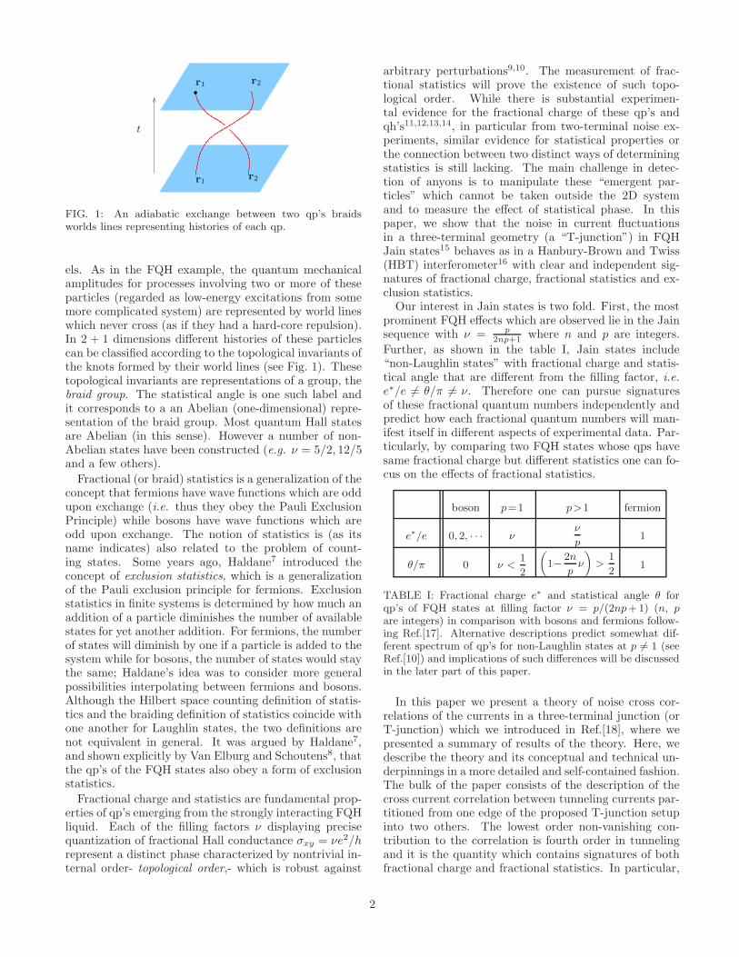
with 0 < θ < π. In the anyonic picture, the statisticalangle corresponds to θ = πqφ/φ0. Laughlin qp’s are aspecific example with q = ν. In order to compute thestatistical angle θ, Arovas et al.5 first considered the theadiabatic process of one qp encircling another. By calcu-lating the Berry phase associated with this process theyshowed that the two qp wave function Ψ(r1, r2) gainsan extra “statistical phase” of ei2νπ in addition to themagnetic flux induced Aharonov-Bohm phase upon encir-cling. An adiabatic exchange of two qp’s can be achievedby moving one qp only half its way around the other andshifting both of them rigidly to end up in interchangedinitial positions. They thus argued that the phase factorpicked up by a two qp joint wave function upon this ex-change process should be precisely half of what it is fora round trip and hence θ = νπ.

From a more general standpoint, anyons are excita-tions which carry a representation of the braid group (seebelow). This is possible both for non-relativistic par-ticles in high magnetic fields (as we will be interestedin here) as well as some field-theoretic relativistic mod-

r1

r1r2

r2

t

FIG. 1: An adiabatic exchange between two qp’s braidsworlds lines representing histories of each qp.

els. As in the FQH example, the quantum mechanicalamplitudes for processes involving two or more of theseparticles (regarded as low-energy excitations from somemore complicated system) are represented by world lineswhich never cross (as if they had a hard-core repulsion).In 2 + 1 dimensions different histories of these particlescan be classified according to the topological invariants ofthe knots formed by their world lines (see Fig. 1). Thesetopological invariants are representations of a group, thebraid group. The statistical angle is one such label andit corresponds to a an Abelian (one-dimensional) repre-sentation of the braid group. Most quantum Hall statesare Abelian (in this sense). However a number of non-Abelian states have been constructed (e.g. ν = 5/2, 12/5and a few others).

Fractional (or braid) statistics is a generalization of theconcept that fermions have wave functions which are oddupon exchange (i.e. thus they obey the Pauli ExclusionPrinciple) while bosons have wave functions which areodd upon exchange. The notion of statistics is (as itsname indicates) also related to the problem of count-ing states. Some years ago, Haldane7 introduced theconcept of exclusion statistics, which is a generalizationof the Pauli exclusion principle for fermions. Exclusionstatistics in finite systems is determined by how much anaddition of a particle diminishes the number of availablestates for yet another addition. For fermions, the numberof states will diminish by one if a particle is added to thesystem while for bosons, the number of states would staythe same; Haldane’s idea was to consider more generalpossibilities interpolating between fermions and bosons.Although the Hilbert space counting definition of statis-tics and the braiding definition of statistics coincide withone another for Laughlin states, the two definitions arenot equivalent in general. It was argued by Haldane7,and shown explicitly by Van Elburg and Schoutens8, thatthe qp’s of the FQH states also obey a form of exclusionstatistics.

Fractional charge and statistics are fundamental prop-erties of qp’s emerging from the strongly interacting FQHliquid. Each of the filling factors ν displaying precisequantization of fractional Hall conductance σxy = νe2/hrepresent a distinct phase characterized by nontrivial in-ternal order- topological order,- which is robust against

arbitrary perturbations9,10. The measurement of frac-tional statistics will prove the existence of such topo-logical order. While there is substantial experimen-tal evidence for the fractional charge of these qp’s andqh’s11,12,13,14, in particular from two-terminal noise ex-periments, similar evidence for statistical properties orthe connection between two distinct ways of determiningstatistics is still lacking. The main challenge in detec-tion of anyons is to manipulate these “emergent par-ticles” which cannot be taken outside the 2D systemand to measure the effect of statistical phase. In thispaper, we show that the noise in current fluctuationsin a three-terminal geometry (a “T-junction”) in FQHJain states15 behaves as in a Hanbury-Brown and Twiss(HBT) interferometer16 with clear and independent sig-natures of fractional charge, fractional statistics and ex-clusion statistics.

Our interest in Jain states is two fold. First, the mostprominent FQH effects which are observed lie in the Jainsequence with ν = p

2np+1 where n and p are integers.

Further, as shown in the table I, Jain states include“non-Laughlin states” with fractional charge and statis-tical angle that are different from the filling factor, i.e.e∗/e 6= θ/π 6= ν. Therefore one can pursue signaturesof these fractional quantum numbers independently andpredict how each fractional quantum numbers will man-ifest itself in different aspects of experimental data. Par-ticularly, by comparing two FQH states whose qps havesame fractional charge but different statistics one can fo-cus on the effects of fractional statistics.

boson p=1 p>1 fermion

e∗/e 0, 2, · · · νν

p1

θ/π 0 ν <1

2

(1−

2n

pν

)>

1

21

TABLE I: Fractional charge e∗ and statistical angle θ forqp’s of FQH states at filling factor ν = p/(2np+1) (n, pare integers) in comparison with bosons and fermions follow-ing Ref.[17]. Alternative descriptions predict somewhat dif-ferent spectrum of qp’s for non-Laughlin states at p 6= 1 (seeRef.[10]) and implications of such differences will be discussedin the later part of this paper.

In this paper we present a theory of noise cross cor-relations of the currents in a three-terminal junction (orT-junction) which we introduced in Ref.[18], where wepresented a summary of results of the theory. Here, wedescribe the theory and its conceptual and technical un-derpinnings in a more detailed and self-contained fashion.The bulk of the paper consists of the description of thecross current correlation between tunneling currents par-titioned from one edge of the proposed T-junction setupinto two others. The lowest order non-vanishing con-tribution to the correlation is fourth order in tunnelingand it is the quantity which contains signatures of bothfractional charge and fractional statistics. In particular,

2

by analyzing the components of the correlation in depth,we pinpoint the role of statistics in various tunneling pro-cesses and discuss implications of the connection betweenbraiding statistics and exclusion statstics.

The paper is organized as follows. In Section II webriefly review the effective theory for edge states devel-oped in Ref. [17] which we will use throughout. In Sec-tion III, we introduce the T-junction setup we are propos-ing and we define the normalized cross current noise tobe calculated purturbatively in Section IV. In Sections Vand VI, we present the time dependent noise and its fre-quency spectrum respectively. We summarized our re-sults and discuss its implications for experiments in Sec-tion VII. In four appendices we present a summary ofthe theory of the edge states that we use here (AppendixA), of the Schwinger-Keldysh technique and conventions(Appendix B), some useful identities for vertex operators(Appendix C), and the unitary Klein factors (AppendixD).

II. AN EFFECTIVE THEORY FOR EDGESTATES

In this section, we summarize the properties of edgestates for the Jain sequence and their associated quasi-particles. While the creation of qp excitations in the 2Dbulk of FQH systems has an associated energy gap, (i.e.FQH liquid is incompressible), the one dimensional (1D)boundary defined by a confining potential can supportgapless excitations10,19. Further there is a striking one-to-one correspondence between qp states in the bulk andat the edge making the FQH liquid holographic19. Giventhat edge states comprise an effective 1D system prop-agating only along the direction dictated by the mag-netic field (a chiral Luttinger liquid10,19), they can bedescribed in terms of chiral bosons using the standardbosonization approach. The edge effective Lagrangiandensity for Jain states, derived from the boundary termof the fermionic Chern-Simons theory20 by Lopez andFradkin17 is given by

L0 =1

4πν∂xφc(−∂tφc − ∂xφc)

+ limvN→0+

1

4π∂xφN (∂tφN + vN∂xφN )

(2.1)

where φc is a right moving charge mode whose speed isset to be vc = 1 (φ− with g = 1/ν and v = 1 case ofAppendix A) and φN is the non-propagating charge neu-tral topological mode obtained as a vN → 0+ limit of arightmover with gN = −1. Note that for the purpose ofregularization and to carefully keep track of short timebehavior which is crucial for ensuring the correct statis-tics, we shall keep a neutral mode speed vN and take thelimit vN → 0 only at the very end.

The normal ordered vertex operator creating a quasi-particle excitation on this edge, with fractional quantumnumbers tabulated in the Table I, is given by17

ψ† ∝ :e−i( 1

pφc+

√1+ 1

pφN )

: ≡ :e−iϕ : (2.2)

where we define a short hand notation ϕ to represent theappropriate linear combination of the charge mode andthe topological mode

ϕ ≡ (1

pφc +

√1 +

1

pφN ). (2.3)

By noting the equal time commutator for the new fieldϕ being

[ϕ(x, t), ϕ(x′, t)] = iπ

(ν

p2− 1

p− 1

)sgn(x− x′)

= −iθ sgn(x− x′)

(2.4)

the quantum numbers of ψ† can be verified as follows.The charge density operator j0 ≡ 1

2π∂xφc measures the

charge of the qp operator since [j0(x), ψ†(x′)] ≡ e∗

e δ(x−x′)ψ†(x′). By expanding the vertex operator Eq. (2.2),this commutator can be calculated order by order to give

[j0(x), ψ†(x′)] =

1

2π[∂xφc(x), e

−i 1p

φc(x′)]

= − 1

2π

i

p∂x[φc(x), φc(x

′)] + · · ·

=1

2π

νπ

p∂xsgn(x− x′) + · · ·

=ν

pδ(x − x′)ψ†(x′),

(2.5)

hence e∗/e = νp . As for statistics, using the Campbell-

Baker-Hausdorff (CBH) formula for exponential of opera-

tors A, eAeB = eBeAe[A,B], the statistical angle of the qpoperator can be calculated via exchange of qp positionsat equal time as the following

ψ†(x)ψ†(x′) = ψ†(x′)ψ†(x)e−[ϕ(x),ϕ(x′)]

= ψ†(x′)ψ†(x)eiθsgn(x−x′),(2.6)

which confirms θ = (1 − 2np ν) modulo 2π.

Combining charge mode and neutral mode propagator,one can obtain the propagator for the field ϕ:

〈ϕ(x, t)ϕ(0, 0)〉

=1

p2〈φc(x, t)φc(0, 0)〉 +

(1 +

1

p

)〈φN (x, t)φN (0, 0)〉

= − ν

p2ln

[τ0 + i(t− x)

τ0

]

+ i limvN→0+

π

2

(1 +

1

p

)sgn(vN t− x).

(2.7)

From Eq. (2.7), one arrives at the following form for theqp propagator at zero temperature (see Appendix C):

3

〈ψ(x, t)ψ†(0, 0)〉= e〈ϕ(x,t)ϕ(0,0)〉

= limvN→0+

[τ0

τ0 + i(t− x)

] ν

p2

e−i π2(1+ 1

p) sgn(vN t−x).

(2.8)

Eq. (2.8) shows that the qp operators have the scalingdimension K

2 = ν2p2 = 1

2p(2np+1) . Further, as τ → 0+,

the limit x→ 0− of Eq. (2.8) becomes

〈ψ(0−, t)ψ†(0, 0)〉 =

∣∣∣∣t

τ0

∣∣∣∣−K

eiθ sgn(t) (2.9)

with the explicit dependence on the statistical angleemerging in the long wavelength limit. This equal po-sition propagator, which explicitly encodes informationon statistics, plays a prominent role in subsequent point-contact tunneling calculations. Most importantly, theamplitude of the propagator Eq. (2.9) is governed by thescaling dimension but the phase is solely determined bythe statistical angle.

Since edge states are gapless excitations, they act aswindows for experimental probes to observe features ofthe FQH droplet. In particular, tunneling between edgesallows a viable access to single qp properties, providedthe tunneling path lie inside the FQH liquid (qp’s onlyexist within the liquid)21.In fact, such tunneling has beensuccessfully used in a geometry hosting a single point con-tact and two edges for the detection of fractional chargethrough shot noise measurements12,13,14. In principle,two edges would suffice for anyonic exchange as well withqp’s from each edge exchanging positions via tunnelingthrough the 2D FQH bulk. However, in order to detectthe phase information, the path of exchange needs to beintercepted, for instance, by inserting a third edge and al-lowing qp exchange between first two edges to go throughthe third edge. This third edge thus acts at once as astage and an “observation deck”. Further, if the first twoedges are each adding/removing qp’s to the third edge,one should be able to see the generalized exclusion prin-ciple in action by probing the third edge. In the nextsection, we propose a “T-junction” interferometer as aminimal realization of such a situation.

III. THE T-JUNCTION SETUP

In our proposed T-junction interferometer of the typeshown in Fig.2, top gates can be used to define and bringtogether three edge states l = 0, 1, 2 which are separatedfrom each other by ohmic contacts. Two edges l = 1 andl = 2 each separately form tunnel junctions with edge 0and upon setting the edge 0 at relative voltage V to thetwo others, qp’s are driven to tunnel between edge 0 andedges 1, 2.

Denoting charge and neutral modes for edge l = 0, 1, 2by φl

c(xl, t) and φlN (xl, t) respectively, each edge state

l in the absence of tunneling (hence the superscript 0)can be described by Lagrangian densities of the form inEq. (2.1):

L(0)l =

1

4πν∂xl

φlc(−∂tφ

lc − ∂xl

φlc) +

1

4π(∂xl

φlN∂tφ

lN )

(3.1)where xl now represents the curvilinear abscissa alongeach edge, and the total Lagrangian density becomes

L(0) =∑

l=0,1,2

L(0l (3.2)

Boson fields φlc and φl

N each have the same properties(such as commutation relations and propegators) as φc

and φN of a single edge described in the Sec. II. Fieldsof different edges commute with each other, i.e.

[φlc/N , φ

mc/N ] = 0, for l 6= m (3.3)

for l,m = 0, 1, 2. Within each edge l, a vertex operatoreiϕl , where ϕl again is a short hand notation ϕ definedin Eq. (2.3) for each edge l, describes a qp excitation

ψ†l in that edge. However, since ϕl’s are constructed to

commute between different edges, we need to introduce

0

1 2

V1

V2

V0

FIG. 2: The proposed T-junction set up. Solid (blue) linesrepresent edge states where the edge state 0 is held at poten-tial V relative to edges 1 and 2, i.e. V0 − V1 = V0 − V2 = V .Dashed (red) lines show paths of two quasiparticle tunnel-ing through a FQH liquid from edge state 0 to edge 1 atx0 = −a/2 ≡ X1 , x1 = 0; from edge 0 to edge 2 atx0 = a/2≡X2, x2 = 0. The direct tunneling between edge 1and 2 is turned off by setting the two edges at equal potential.

4

unitary Klein factors Fl with the appropriate algebra, asshown in the Appendix D, to give the correct qp statisticsupon exchange between different edges. Hence, we have

ψ†l =

1√2πa0

Flei(

1p

φlc+√

1+ 1p

φlN

)

≡ 1√2πa0

Fleiϕl , (3.4)

where a0 is the short distance cutoff and the Klein factorsobey the statistical rules

FlFm = e−iαlmFmFl (3.5)

where αlm = −αml and α02 = α21 = −α10 = θ. No-tice the Klein factors do not affect the statistics betweenoperators on the same edge since αll = 0 from the re-quirement αlm = −αml.

Now, if we set the the distance between two tunnelingpoints on edge 0 to be a small positive real number a(which we later send to zero) and the tunneling point onedge 1, 2 to be the origin for the abscissa coordinate ofedge 1, 2, then qp’s tunnel at two locations , x0 =−a/2≡X1 and x0 = a/2 ≡X2 on edge 0 and at x1 = 0, x2 = 0

on edges 1, 2. The operator Vj(t) which tunnels one qpfrom the edge 0 to edges j = 1, 2 at time t can then bewritten in the following form:

V †j (t) ≡ ψ0(Xj , t)ψ

†j (0, t)

= F0F−1j eiϕ0(Xj ,t)e−iϕj(0,t).

(3.6)

The additional term in the Lagrangian due to the pres-ence of the tunneling can be written as Lint = Lint,1 +Lint,2

22,23 with tunneling term involving edges j = 1, 2given by

Lint,j(t) = −Γj V†j (t) + h.c. , (3.7)

where Γj is the tunneling amplitude between edges 0 andj= 1, 2. The non-equilibrium situation of setting a con-stant DC voltage bias V between edges 0 and j corre-sponds to substituting Γj by Γje

−iω0t in Eq. (3.7), wherethe Josephson frequency is explicitly determined by thefractional charge to be ω0 ≡ e∗V/ℏ (the Peierls substitu-tion22,24,25). Using the Heisenberg equations of motionfor the total charge Ql =

∫dxlj0l(xl) of edge l where

j0l(xl) = 12π∂xφ

lc is the charge density operator for edge

l, as was done by Chamon et al.24, 25 for Laughlin states,one can show that the tunneling current operator, Ij(t),from edge 0 to edge j is given by

Ij(t) = ie∗

~Γj(e

iω0tV †j − e−iω0tVj),

≡ ie∗∑

ǫ=±

ǫ Γj eiǫω0t V

(ǫ)j ,

(3.8)

where we assumed Γj to be real and introduced the no-

tation V †j ≡ V

(+)j and Vj ≡ V

(−)j , i.e.,

V(ǫ)j (t) = (F0F

−1j )ǫ eiǫϕ0(Xj ,t) e−iǫϕj(0,t), (3.9)

to represent the summation over hermitian conjugates ina compact form. Notice that ǫ = + corresponds to a qptunneling from the edge j to 0 and ǫ = − corresponds toa reverse direction tunneling.

We treat the non-equilibrium situation within theSchwinger-Keldysh formalism22,23,24,25,26,27,28 for com-puting expectation values of operators. As a simple ex-ample, the expectation value of the current on edge jtakes the following form up to a normalization factor

〈Ij〉 =1

2

∑

η=±

〈TK Ij(tη)ei

∫K

Lint,j(tj)dtj 〉0 (3.10)

where η labels the branch of the Keldysh contour: η=+for the forward branch (t = −∞ → ∞) and η = − forthe backward branch (t=∞ → −∞). TK indicates thatthe operators inside brackets should be contour orderedbefore taking the expectation value, and 〈〉0 indicates theexpectation value with respect to the free action S0 =∫

Kdt∫d3xL0 where the free Lagrangian density L0 was

given in Eq. (3.2).Our goal is to identify a measurable quantity that dis-

tinctly captures the role of the statistical angle θ whichfeatures in the single qp operator shown in Eq. (2.6). Thenormalized cross correlation (noise) S(t) between tunnel-ing current fluctuations (∆Il = Il − 〈Il〉):

S(t− t′) ≡ 〈∆I1(t)∆I2(t′)〉〈I1〉〈I2〉

(3.11)

turns out to be the simplest quantity that can exhibit thesubtle signatures of statistics and distinguish them fromthose of fractional charge. In fact, in contrast to shotnoise, this cross current correlation S(t − t′) carries sta-tistical information even at the lowest non-trivial order,which we calculate perturbatively in the next section.

IV. PERTURBATIVE CALCULATION

In this section, we perform a detailed analysis ofthe normalized cross correlation at fourth (lowest non-vanishing) order in tunneling. We calculate the two pointcorrelation and four point correlation functions requiredto calculate the cross correlation in terms of edge stateproperties. We analyze the detailed behavior of the crosscorrelation over different Keldysh time domains and pin-point the effects of statistics, specifically drawing the con-nection between braiding statistics and exclusion statis-tics. We show that cross correlation can be expressedin terms of two universal scaling functions and that thestatistical dependence ultimately takes on a remarkablysimple form.

It must be remarked that since the perturbation in-troduced in Eq. (3.7) is relevant in the renormalizationgroup sense, perturbation theory is valid only under cer-tain conditions. Specifically, perturbation holds as longas energies involved, such as voltage and temperature,are higher than a cross-over energy scale proportional

5

to Γ1

1−K . For energies much lower than this cross-overscale, qp tunneling between edges becomes large enoughto break the Hall droplet into smaller disconnected re-gions and one needs an appropriate dual picture to prop-erly address the strong coupling fixed point. For observ-ing the effects of statistics as prescribed by the correlationcalculated here, it is imperative that the system remains

in the perturbative regime.

The un-normalized cross correlation 〈I1〉〈I2〉S(t−t′) =〈∆I1(t)∆I2(t′)〉, where 〈〉 represents expectation valuewith respect to the full Lagrangian in the presence oftunneling events, can be written in terms of expectationvalues with respect to the free theory 〈〉0 as

〈I1〉〈I2〉S(t− t′) =1

4

∑

η,η′

〈TK I1(tη)I2(t

′η′

) ei∫

KLint,1(t1)dt1+i

∫K

Lint,2(t2)dt2〉0

− 1

4

∑

η,η′

〈TK I1(tη)ei

∫K

Lint,1(t1)dt1〉0〈TK I2(t′η′

)ei∫

KLint,2(t2)dt2〉0.

(4.1)

By expanding the exponentials in Eq. (4.1), we cancalculate the cross correlation perturbatively in the tun-neling amplitude Γj . Since the tunneling operator is rel-evant in the RG sense (its scaling dimension is less than1), the perturbation theory will break down in the in-frared (IR) limit. However, the finite temperature inour case provides a natural IR cutoff making this per-turvative calculation meaningful. In fact, we will show

in the following sections that the strongest statistical de-pendence is obtained at temperatures comparable to thebias voltage.

Clearly the lowest non-vanishing term in the perturba-tion expansion is of order (Γ1Γ2)

2. Using the expressionfor the tunneling current operator in Eq. (3.8), the firstterm of Eq. (4.1) to this order can be written as

〈I1(t)I2(t′)〉(2) ≡ (−i)2(ie∗)214

∑

η,η′,η1,η2

∑

ǫ,ǫ′

ǫǫ′η1η2|Γ1Γ2|2∫dt1dt2e

iǫω0(t−t1)+iǫ′ω0(t′−t2)

× 〈TK V(ǫ)1 (tη)V

(ǫ′)2 (t′η

′

)V(−ǫ)1 (tη1

1 )V(−ǫ′)2 (tη2

2 )〉0(4.2)

where we used the fact that the Keldysh contour time-integral in the exponent can be represented using thecontour branch index η′

∫

K

dt =∑

η′=±

η′∫dt (4.3)

and the charge neutrality condition discussed in the Ap-pendix C which enforces ǫ1 = −ǫ and ǫ2 = −ǫ′. Similarly,the expectation value of the current for the second termof Eq. (4.1) becomes

〈I1〉(2) =1

2

∑

ǫ=±1

∑

η,η1

(−i)(ie∗)ǫη1∫dt1

[

|Γ1|2eiǫω0(t−t1)〈TK V(ǫ)1 (tη)V

(−ǫ)1 (tη1

1 )〉0]

(4.4)

Putting Eq. (4.2) and Eq. (4.4) together, we arrive at thefollowing expression for the lowest non-vanishing term ofthe un-normalized cross current correlation

6

〈I1〉〈I2〉S(2)(t− t′) =1

4(e∗)2

∑

η,η′,η1,η2

∑

ǫ,ǫ′

ǫǫ′η1η2|Γ1Γ2|2∫dt1dt2e

iǫω0(t−t1)+iǫ′ω0(t′−t2)

×[〈TK V

(ǫ)1 (tη)V

(ǫ′)2 (t′η

′

)V(−ǫ)1 (tη1

1 )V(−ǫ′)2 (tη2

2 )〉0

−〈TKV(ǫ)1 (tη)V

(−ǫ)1 (tη1

1 )〉0〈TK V(ǫ′)2 (t′η

′

)V(−ǫ′)2 (tη2

2 )〉0].

(4.5)

We now evaluate the two point function and the fourpoint function, and then combine them to obtain a sim-plified formula for 〈I1〉〈I2〉S(2)(t− t′) from Eq. (4.5).

A. The two point function

Using Eq. (3.6) and the result of Appendix C to cal-culate the chiral boson vertex correlation function, wefind

〈TKV(ǫ)1 (tη)V

(−ǫ)1 (tη1

1 )〉0= (F0F

−11 )ǫ(F0F

−11 )−ǫ〈TKe

iǫϕ0(X1,tη)e−iǫϕ0(X1,tη11

)〉× 〈TKe

iǫϕ1(0,tη)e−iǫϕ1(0,tη11

)〉 (4.6)

= exp[Gη,η1(0, t−t1)] exp[Gη,η1

(0, t−t1)] (4.7)

where Gη,η′(x−x′, t− t′) ≡ 〈TKϕl(x, tη)ϕl(x

′, t′η′

)〉0 isthe Keldysh ordered and regulated ϕl propagator for alll which will be discussed below in detail for both zerotemperature and finite temperatures. Here we also usedthe fact that ϕl’s are independent from each other fordifferent l’s. Notice that the Klein factor contributionsimply becomes an identity for a two point function of

the tunneling operator V1. Hence, Klein factors are notnecessary in calculations involving two point functionsalone, and in fact, this is the reason that the lowest or-der contribution to shot noise does not contain statisticalinformation. However, as we show below, Klein factorshave non-trivial contributions in the four point functionwhich appears in the first term of Eq. (4.1).

We now focus on the form of Gη,η′(−a, t − t′) in thelimit a→ 0+. From the detailed analysis of Appendix B,the contour ordered propagators for φc and φN takes thefollowing forms at finite temperatures:

〈TKφc(x, tη)φc(x

′, t′η′

)〉

= −ν ln

[sinπ

β[τ0 + iχη,η′(t− t′){(t−t′)−(x− x′)}]πτ0

β

]

(4.8)

〈TKφN (x, tη)φN (x′, t′η′

)〉= lim

vN→0+−iπ

2χη,η′ sgn[vN (t− t′) − (x − x′)]. (4.9)

Hence the contour ordered propagator for ϕ representedby G in Eq. (4.7) and Eq. (4.18) can be written as

Gη,η′(−a, t− t′) = − ν

p2ln

[sinπ

β[τ0 + iχη,η′(t− t′)(t−t′ + a)]πτ0

β

]+ lim

vN→0+iπ

2

(1

p+ 1

)χη,η′(t− t′) sgn[vN (t− t′) + a]

(4.10)

For the case of interest,i.e., a→ 0+ in the limit τ0 → 0+,the above takes the following form (See Appendix B):

Gη,η′(0−, t− t′) = lnC(t− t′; T,K)

+ iθ

2χη,η′(t− t′) sgn(t− t′). (4.11)

where we have introduced a notation for the amplitudeof the qp propagator that depends on the temperature Tand the scaling dimension K = ν/p2:

C(t; T,K) ≡ (πτ0)K

|sinhπkBT t|K, (4.12)

and defined

χη,η′(t− t′) ≡(η + η′

2sgn(t− t′) − η − η′

2

). (4.13)

We can now calculate the expectation value of the tun-neling current 〈I1〉 of Eq. (4.4) to order O(Γ2

1) usingEq. (4.7) and Eq. (4.10),

〈I1(tη)〉(2) = e∗|Γ1|2∑

ǫ

ǫ

∫dt1e

iǫω0(t−t1)Υ(θ)C(t− t1)2

(4.14)

7

with the statistical factor

Υ(θ) =

(∑

η1

η1eiθχη,η1

(t−t1) sgn(t−t1)

)= 2i sin θ (4.15)

Notice that the resulting 〈I1(tη)〉 is independent of η andis a constant independent of t, as applicable for a steady

state current.

B. The four point function

Following a procedure similar to the one that led up toEq. (4.7), we find that the four point function becomes

〈TKV(ǫ)1 (tη)V

(ǫ′)2 (t′η

′

)V(−ǫ)1 (tη1

1 )V(−ǫ′)2 (tη2

2 )〉0= 〈TKe

iǫϕ0(X1,tη)eiǫ′ϕ0(X2,t′η′)e−iǫϕ0(X1,t

η11

)e−iǫ′ϕ0(X2,tη22

)〉0〈TKeiǫϕ1(0,tη)e−iǫϕ1(0,t

η11

)〉0× 〈TKe

iǫ′ϕ2(0,t′η′)e−iǫ′ϕ2(0,t

η22

)〉0〈TK(F0F−11 )ǫ(F0F

−12 )ǫ′(F0F

−11 )−ǫ(F0F

−12 )−ǫ′〉0 (4.16)

= e[Gη,η1(0,t−t1)+Gη′,η2

(0,t′−t2)+ǫǫ′Gη,η2(−a,t−t2)+ǫǫ′Gη′η1

(−a,t′−t1)−ǫǫ′Gηη′ (a,t−t′)−ǫǫ′Gη1η2(−a,t1−t2)]

× eGηη1(0,t−t1)eGη′η2

(0,t′−t2)〈TK(F0F−11 )ǫ(F0F

−12 )ǫ′(F0F

−11 )−ǫ(F0F

−12 )−ǫ′〉0 (4.17)

= e2[Gηη1(0,t−t1)+Gη′η2

(0,t′−t2)] eǫǫ′[Gη,η2

(−a,t−t2)+Gη′η1(a,t′−t1)]

eǫǫ′[Gηη′ (−a,t−t′)+Gη1η2(−a,t1−t2)]

〈TK(F0F−11 )ǫ(F0F

−12 )ǫ′(F0F

−11 )−ǫ(F0F

−12 )−ǫ′〉0 (4.18)

where we used Eq. (C6) for the case N = 4 to calculatethe four vertex correlator for the second equality andused the fact that X1 −X2 = −a.

The factor involving four sets of Klein factors of theform (F0F

−1j )± in the Eq. (4.18) has to be appropriately

rearranged through proper exchange rules, Eqs. (D2) and

(D5), as the tunneling operators Vj(tη)’s get rearranged

for Keldysh contour ordering. Since contour orderingdepends on time arguments of the tunneling operators,Klein factors effectively become endowed with dynamicsin the sense that where each of these four times fall onthe contour determines whether Klein factors associatedwith tunneling at each time have to be moved or not23.In order to rearrange four sets of combined Klein fac-tors of the form (F0F

−1j )ǫ(tη) involved in Eq. (4.18), we

have to take six different possible pairs and contour orderwithin each pair. This process can be thought of as a full“contraction” where pairs of Klein factors can be treatedakin to propagators.

These contour ordered Klein factor “propagators” werecalculated in Appendix D to be

〈TK(F0F−11 )ǫ(tη)(F0F

−12 )ǫ′(t′η

′

)〉0= eiǫǫ′ θ

2sgn(X1−X2)χη,η′ (t−t′) = e−iǫǫ′ θ

2χη,η′ (t−t′) (4.19)

〈TK(F0F−12 )ǫ(tη)(F0F

−11 )ǫ′(t′η

′

)〉0= eiǫǫ′ θ

2sgn(X2−X1)χη,η′ (t−t′) = e−iǫǫ′ θ

2χη′,η(t′−t) (4.20)

(4.21)

where χη,η′(t) is defined in Eq. (4.13). Further using the

fact that F0F−1j commutes with itself gives

〈TK(F0F−1j )ǫ(tη)(F0F

−1j )−ǫ′(t′η

′

)〉0 = 1. (4.22)Expressing the Klein factor contribution in Eq. (4.18) interms of the six possible pairs and using their forms givenby Eq. (4.21) and Eq. (4.22) simplifies it to the form

e−iǫǫ′ θ2χη,η2

(t−t2)e−iǫǫ′ θ2χη1,η′ (t1−t′)

e−iǫǫ′ θ2χη,η′ (t−t′)e−iǫǫ′ θ

2χη1,η2

(t1−t2). (4.23)

Hence, we can rewrite the four point function ofEq. (4.18) as the following:

8

〈TKV(ǫ)1 (tη)V

(ǫ′)2 (t′η

′

)V(−ǫ)1 (tη1

1 )V(−ǫ′)2 (tη2

2 )〉0

= e2[Gηη1(0, t−t1)+Gη′η2

(0, t′−t2)] eǫǫ′[Gη,η2

(−a, t−t2)−i θ2χη,η2

(t−t2)+Gη1,η′ (−a,t1−t′)−i θ2χη1,η′ (t1−t′)]

eǫǫ′[Gη,η′(−a, t−t′)−i θ2χη,η′ (t−t′)+Gη1,η2

(−a, t1−t2)−i θ2

χη1,η2(t1−t2)]

(4.24)

where we used the fact that Gη,η′(x − x′, t − t′) =Gη′,η(x′−x, t′−t), as it is pointed out in the Appendix B,to replace Gη′,η1

(a, t′ − t1) by Gη1,η′(−a, t1 − t′).

Furthermore, observing the following,

Gη,η′(0−, t− t′) − iθ

2χη,η′(t− t′)

= −K ln

∣∣∣∣∣∣

sinh(

π(t−t′)β

)

πτ0

β

∣∣∣∣∣∣+ i

θ

2η(1 − sgn(t− t′))

(4.25)

= Gη,−η(0−, t− t′), (4.26)

where we have used Eq. (4.11) and Eq. (4.13), the fourpoint function of Eq. (4.24) further simplifies to the finalform

〈TK V(ǫ)1 (tη)V

(ǫ′)2 (t′η

′

)V(−ǫ)1 (tη1

1 )V(−ǫ′)2 (tη2

2 )〉0= e2[Gηη1

(0, t−t1)+Gη′η2(0, t′−t2)]

× eǫǫ′[Gη,−η(0−, t−t2)+Gη1,−η1(0−,t1−t′)]

eǫǫ′[Gη,−η(0−, t−t′)+Gη1,−η1(0−, t1−t2)]

(4.27)

≡ (πτ0)2K

∣∣∣sinh π(t−t1)β

∣∣∣2K

(πτ0)2K

∣∣∣sinh π(t′−t2)β

∣∣∣2K

×

∣∣∣sinh π(t1−t2)β

∣∣∣ǫK ∣∣∣sinh π(t−t′)

β

∣∣∣ǫK

∣∣∣sinh π(t1−t′)β

∣∣∣ǫK ∣∣∣sinh π(t−t2)

β

∣∣∣ǫKeiΦ

η,η′,η1,η2ǫ

(t,t′,t1,t2)

(4.28)

where we defined ǫ ≡ ǫǫ′ noting that Eq. (4.24) dependsonly on the product ǫǫ′ and collected all contributions to

the phase factor by defining the following function

Φη,η′,η1,η2

ǫ (t, t′, t1, t2)

≡ θχη,η1(t− t1) + θχη′,η2

(t′ − t2)

− ǫθ

2

[η sgn(t− t2) − η sgn(t− t′)

]

− ǫθ

2

[η1 sgn(t1 − t′) − η1(t1 − t2)

](4.29)

= −η θ2{ sgn(t− t1) + ǫ sgn(t− t2)

− ǫ sgn(t− t′) − 1} + η′θ

2{1 − sgn(t′ − t2)}

− η1θ

2{− sgn(t− t1) + ǫ sgn(t1 − t′)

− ǫ sgn(t1 − t2) − 1} + η2θ

2{1 + sgn(t′ − t2)}.

(4.30)

S

t1 t2

(a)

O

t1 t2

(b)

FIG. 3: Virtual tunneling events taking place at all times t1and t2 allowed by causality contribute to the noise (tunnel-ing current cross-correlation) S(t) in the lowest non-vanishingorder. Solid (red) lines show paths of two quasiparticles tun-neling through a FQH liquid from one edge state to two others(consitituting I1 and I2) and dashed (magenta) lines representvirtual tunneling events. Depending on the relative orienta-tion of the currents (or equivalently of the virtual processes)there are two cases: (a) the case S in which two currents arein the same orientation (ǫ = +1 in the text) and (b) the caseO in which two currents are in the opposite direction (ǫ = −1in the text).

Note that ǫ ≡ ǫǫ′ depends only on the relative direc-tions of tunneling, that is ǫ = +1 for correlations betweencontributions to I1 and I2 in the same orientation (ǫ = ǫ′)and ǫ = −1 for correlations between contributions to I1and I2 in the opposite orientation (ǫ = −ǫ′). Each caseof ǫ = ± is illustrated in Fig. 3 labeled S/O respectively.The fact that the phase factor Φ depends on these rela-tive orientations allows us to understand the statistical

9

angle dependent contribution to the noise in connectionwith exclusion statistics7 as we will discuss in the nextsection. Another important observation to be made inEq. (4.30) is that the time dependence of the phase fac-tor is such that it only depends on the sign of various timedifferences. Hence as we integrate over virtual times t1and t2, to evaluate 〈I1(t)I2(0)〉 according to Eq. (4.2),the domain of integration in (t1, t2) space can be dividedinto sub-domains as shown in Fig. 4 and the phase factorsfor a given set of Keldysh branch indices η’s and relativeorientation of tunneling ǫ may be computed. Since inte-gration is additive, we can consider each domain’s con-tribution separately and later add them up to unravelthe effect of the phase factor. A simple analysis to follow

shows that large parts of the (t1, t2) space do not con-tribute to the integral due to vanishing summation overη’s. The remaining domains can then be assigned differ-ent values of overall constant from the summation overthe phase factor.

C. The normalized noise

Putting Eq. (4.28) back into Eq. (4.2) for the O(Γ21Γ

22)

term of the current-current correlation and setting t′ =0 (the expression has time translational invariance) andtaking t > 0, we obtain for 〈I1(t)I2(0)〉(2)

〈I1(t)I2(0)〉(2)

= (−i)2(ie∗)2∑

η1,η2

∑

ǫ,ǫ′

ǫǫ′η1η2|Γ1Γ2|2∫dt1dt2 e

iǫω0(t−t1)−iǫ′ω0t2 eiΦη,η′,η1,η2ǫ (t,0,t1,t2)

× (πτ0)2K

∣∣∣sinh π(t−t1)β

∣∣∣2K

(πτ0)2K

∣∣∣sinh πt2β

∣∣∣2K

∣∣∣sinh π(t1−t2)β

∣∣∣K ∣∣∣sinh πt

β

∣∣∣K

∣∣∣sinh πt1β

∣∣∣K ∣∣∣sinh π(t−t2)

β

∣∣∣K

ǫǫ′

= 2e∗2|Γ1Γ2|2∑

ǫ=±

∫dt1dt2 ǫ cos[ω0(t− t1 − ǫt2)]

×(

∑

η1,η2=±

η1η2eiΦ

η,η1,η2ǫ

(t,0,t1,t2)

)(πτ0)

2K

∣∣∣sinh π(t−t1)β

∣∣∣2K

(πτ0)2K

∣∣∣sinh πt2β

∣∣∣2K

∣∣∣sinh π(t1−t2)β

∣∣∣K ∣∣∣sinh πt

β

∣∣∣K

∣∣∣sinh πt1β

∣∣∣K ∣∣∣sinh π(t−t2)

β

∣∣∣K

ǫ

(4.31)

where we separated the summation over Keldysh branchindices

∑η,η′,η1,η2

from the rest of the integrand us-ing the fact that Keldysh branch index dependence en-ters the expression only through the total phase fac-tor Φ. To get the second equality, we first used theidentities

∑ǫ,ǫ′=± =

∑ǫ,ǫ=± (ǫ ≡ ǫǫ′) and then used

eiǫω0(t−t1)−iǫ′ω0t2 = eiǫω0{t−t1−ǫǫ′t2}.Now evaluating the summation over η’s:

∑

η1,η2=±1

η1η2 eiΦ

η,η′,η1,η2ǫ

(t,0,t1,t2) (4.32)

for different ranges of (t1, t2),allows us to extract thestatistical angle θ dependence of the cross correlation.To do so, we begin by noting that the expression for ΦEq. (4.30) takes a constant value for different domainsand hence the sum over η1, η2 = ±1 in the brackets ofEq. (4.31) can be independently evaluated prior to evalu-ating the integral if the virtual time (t1, t2) space is splitinto appropriate sub-domains. Consequently, we makethe following observations:

1. We first note that Φη,η′,η1,η2

ǫ (t, 0, t1, t2) is indepen-

dent of η2 for t2 > 0. Since∑

η2=±1 η2 = 0,

the expression of Eq. (4.32) vanishes identically fort2 > 0. Hence the only non-zero contribution tothe integral comes from t2 < 0.

2. A similar consideration for the summation over η1for t1 > t allows us to limit the integration range

to t1 < t since Φη,η′,η1,η2

ǫ (t, 0, t1>t, t2< 0) is inde-pendent of η1.

3. The above analysis reflects the fact that only vir-tual times prior to the times of tunneling eventscan affect the correlation between tunneling eventsdue to causality (thus acting as a check that ourimplementation of the Keldysh formalism for Kleinfactors is faithful in respecting causality).

4. Now we are left only with the region {(t1, t2)| t1<t, t2 < 0} which is shaded in the Fig. 4. In thisregion, the phase of Eq. (4.30) simplifies to

Φη,η′,η1,η2

ǫ =θ

[η1

{1+ ǫ

(sgn(t1−t2)− sgn(t1)

2

)}+η2

]

(4.33)

10

t

t1

t2

R1

R3

R2

FIG. 4: Subdomains of integration in the virtual time (t1, t2)space as it is defined in Eq. (4.34). Only the virtual times(t1, t2) that lie in the three shaded subdomains R1, R2, andR3 give non-zero contribution to the cross current correlationEq. (4.5) due to causality which is encoded in the Keldyshformalism.

where we used the fact that we are interested inthe case t > 0. From this expression, which is inde-pendent of η and η′, we can identify three domainsthat contribute to the integral of Eq. (4.31):

R1 ≡ {(t1, t2)| t1<t2<0},R2 ≡ {(t1, t2)| t2<t1<0},R3 ≡ {(t1, t2)| t2<0<t1<t}

(4.34)

as we depicted in Fig. 4.

5. Φη,η1,η2

ǫ (t, 0, t1, t2) can now be considered as a func-tion that depends on the domain Rζ (ζ = 1, 2, 3)which can be evaluated to give

Φη,η′,η1,η2

ǫ [R1] = θ(η1 + η2), (4.35)

Φη,η′,η1,η2

ǫ [R2] = θ{η1(1 + ǫ) + η2}, (4.36)

Φη,η′,η1,η2

ǫ [R3] = θ(η1 + η2). (4.37)

It is worth noting that Φǫ has an explicit depen-dence upon ǫ only in the domain R2. However,since Φη,η1,η2

ǫ [R2] becomes independent of η1 forǫ = −1, the sum Eq. (4.32) will once again vanish.Hence we find that only the case ǫ = +1, wherethe calculated correlation is between the tunnelingprocesses with same orientations (case S of Fig. 3),contributes to the part of the integral Eq. (4.31)coming from the domain R2. Later we will discussthe implication of this observation in more detail.

6. Finally we can evaluate the phase factor summa-tion over contour branch indices Eq. (4.32) for eachregions using Eqs. (4.35-4.37) as the following:

For R1 :∑

η1η2=±1η1η2eiΦ

η,η′,η1,η2ǫ [R1] =

∑

η1,η2=±1

η1η2eiθ(η1+η2) = −4 sin2 θ (4.38)

For R2 :∑

η1η2=±1η1η2eiΦ

η,η′,η1,η2ǫ [R2] =

∑

η1,η2=±1

η1η2eiθ(η1(1+ǫ)+η2) =

{− 4 sin2 θ(2 cos θ) for ǫ=+1

0 for ǫ=−1

}(4.39)

For R3 :∑

η1η2=±1η1η2eiΦ

η,η′,η1,η2ǫ [R3] =

∑

η1,η2=±1

η1η2eiθ(η1+η2) = −4 sin2 θ. (4.40)

At last, we can utilize the observations we made aboveto rewrite the four-point contribution to the noise S(t)spelled out in Eq. (4.31) in the following form

〈I1(t)I2(0)〉(2)

= −8 sin2 θ e∗2|Γ1Γ2|2∑

ǫ=±

∫

R1,R3

dt1dt2ǫ cosω0(t−t1−ǫt2)

× (C(t− t1)C(t2))2

[C(t1)C(t− t2)

C(t1 − t2)C(t)

]ǫ

− 16 sin2 θ cos θ e∗2|Γ1Γ2|2∫

R2

dt1dt2 cosω0(t− t1 − t2)

× (C(t− t1)C(t2))2

[C(t1)C(t− t2)

C(t1 − t2)C(t)

](4.41)

In Eq. (4.41) the statistical angle dependence has beenextracted out and we found an additional factor of 2 cos θin the contribution from the domain R2 which does notoccur in the contributions from domains R1 and R3. Wenote that this contribution rises only from the case S ofFig. 3 (tunneling processes in the same orientation, i.e.ǫ = +1) as it is shown explicitly in the second equalityof Eq. (4.41) by the value of ǫ being set to +1 in thecontribution (the second term).

To complete our analysis, we now turn to the productof two point functions (the second term of Eq. (4.1)).From Eq. (4.14), the second term of Eq. (4.1) to orderO(Γ2

1Γ22) becomes

11

〈I1(t)〉〈I2(0)〉(2)

= −4 sin2 θ e∗2|Γ1Γ2|2∑

ǫ,ǫ′=±

ǫǫ′∫dt1dt2 e

iǫω0(t−t1)−iǫ′ω0(t2)C(t− t1)2C(t2)

2.(4.42)

Finally, putting all of the above together, the normal-ized noise (cross current correlation) is found to be of thefollowing form

S(t; T/T0,K) =∑

ζ=1,3

∑

ǫ=±

S ǫζ(t; T/T0,K) − 1

+ 2 cos θ S+2 (t; T/T0,K), (4.43)

where S ǫζ(t) for all values of ǫ = ± and ζ = 1, 2, 3 is

defined by an integral over domain Rζ for contributionswith relative orientation of tunneling ǫ normalized by theproduct of the average tunneling current

S ǫζ(t; T/T0,K) ≡

ǫ

∫

Rζ

dt1dt2 cos(t− t1 − ǫt2)(C(t− t1)C(t2)

)2[C(t1)C(t− t2)

C(t1 − t2)C(t)

]ǫ

∑

ǫ′=±1

∑

ζ′=1,2,3

∫

Rζ′

dt1dt2 cos[t− t1 − ǫ′t2]C(t− t1)2C(t2)

2(4.44)

where we defined the dimensionless time t ≡ ω0t and alsointroduced a notation for the temperature equivalent tothe Josephson frequency to be T0 ≡ ℏω0/kB and usedthe fact that C(t;T,K) = C(t;T/T0,K) from Eq. (4.12).Note that since we chose to study the normalized noise,all cutoff dependence and tunneling amplitude depen-dence in the noise is eliminated through normalizationsince they enter as common factors for numerator anddenominator of Eq. (4.44).

D. Discussion

Now we can define two scaling functions A and B thatdepend on the scaling dimension K, the Josephson fre-quency ω0 = e∗V/ℏ (or T0) and the temperature as

A(ω0t; T/T0,K) ≡∑

ζ=1,3

∑

ǫ=±

S ǫζ(ω0t; T/T0,K) − 1

B(t; T/T0,K) ≡ 2S+2 (ω0t; T/T0,K). (4.45)

We can thus rewrite Eq. (4.43) as a sum of two scalingfunctions, corresponding to a “direct term” and an “ex-change term” which depends explicitly on cos θ:

S

(ω0t;

T

T0,K

)= A

(ω0t;

T

T0,K

)

+ cos θ B

(ω0t;

T

T0,K

), (4.46)

where T0 = ℏω0/kB. Hence we were able to extract thestatistical angle dependence of the noise in the form ofthe factor of cos θ in the second term while both of thescaling functions A and B do not depend on the statistics.Eq. (4.46) is the key result of this paper. One can gainfurther insight by recognizing the fact that the domainR1 (which contributes to A) and R2 (which contributesto B) are related to each other via exchange of virtualtimes t1 and t2 (See Fig. 4). In the following we discussthe physics behind the factor cos θ in Eq. (4.46) with aneye towards bridging the connection between exclusionstatistics and exchange statistics in our setup.

This expression displays a number of noteworthy prop-erties:

a. This finite temperature result is applicable to allJain states (in contrast to recent zero temperatureresults on Laughlin states22,29) and it is a universalscaling function to the lowest order in perturbationtheory which is valid provided the tunneling currentis small compared to the Hall current.

b. Fractional charge and statistics play fundamentallydistinct roles, each entering Eq. (4.46) through dif-ferent features: fractional charge through ω0 =e∗V/ℏ and fractional statistics through the cos θfactor.

c. Given that for Laughlin states θ < π/2 and cos θ >0, the exchange term in Eq (4.46) provides largelypositive (“bunching”, boson-like) contributions to

12

the noise whereas for non-Laughlin states withθ > π/2, its contribution is largely negative (“anti-bunching”, fermion-like).

d. The fact that only case S, of Fig. 2, contributesto this factor can be viewed as a manifestation ofa generalized exclusion principle7 since the virtualprocesses in this case involves adding a qp to edge0 in the presence of another. It is noteworthy thatwe arrived at an observable consequence of a gen-eralized exclusion principle given that Eq. (4.46))was derived using anyonic commutation rules pre-scribed by braiding statistics5.

A few remarks are in order here. For the function inEq. (4.46) to be observable, given that it is the ratiobetween the cross-current correlations and the averagevalues of the currents involved, the former needs to beat least comparable to the latter. As mentioned above,the form of the function only takes into account the low-est order terms in tunneling; when higher order termsbecome important, the function no longer remains uni-versal in that it exhibits an explicit dependence on tun-neling amplitudes. We assumed that tunneling from edge0 occurred from a single point. In our calculations, wecould have in principle retained the separation scale ’a’for points from which qps tunnel into edges 1 and 2, re-spectively. Then, 1/a would enter the problem as anotherenergy scale. The scaling function would depend on an-other parameter ω0a and the cross-current correlationswould decay with separation length.

As one might expect from the simple form of the sta-tistical angle dependence of Eq. (4.46), this expressioncan be understood in terms of simple pictures in whichthe setup simultaneously acts as an accessible stage forexchange processes and a testbed for generalized exclu-sion.

To see that the form of Eq. (4.46) derives directly fromexchange of qp’s between edge 1 and edge 2 via edge 0, wefirst note that information regarding anyonic exchangestatistics and related time ordering of events is carriedas a phase factor in the qp propagators. Contour or-dering of events and associated time-dependent shufflingis completely contained in this exchange statistics phasefactor. The following analysis of tunneling events andtheir effect on the phase factor not only shows that thesimple cos θ factor in Eq. (4.46) naturally emerges fromthe events associated with exchange statistics, but thatit is also a manifestation of exclusion statistics.

Given that causality constrains lowest order virtualprocesses to occur at times t1 and t2 within domainsR1, R2 and R3 of Fig. 4, a qp/qp from edge 1 cannotexchange with a qp/qh from edge 2 when t1 > 0 (domainR3) since qp/qh tunnels between edge 2 and edge 0 viavirtual process at time t2 < 0 and back at time 0 beforeanything happens between 1 and 0. Hence it is clear asto why S ǫ

3 coming from domain R3 contributes to A andan uncorrelated two-point piece is subtracted out.

Now for domains R1 and R2, there is an overlap |t1−t2|

in the times during which qp/qh’s from edge 1 and edge2 stay in edge 0 and hence can experience statistics in-duced interference. Between R1 and R2, the only pairsof time whose relative orders change from one domain tothe other is t1 and t2 and hence R1 and R2 are relatedto each other via exchange of entities involved in the vir-tual processes occurring at t1 and t2. For both domains,depending on the relative orientations of the currents,the virtual tunneling processes leave two distinct pairs ofobjects at edge 0 as shown in Fig. 3.

In case S (ǫ = +1), where I1 and I2 have the same ori-entation , the entities left behind are a pair of two qp’s.Hence the domain R2 is related to the domain R1 viaexchange of these two identical particles. This exchangebetween two qp’s brings in an additional phase factor ofeiη1θ in Eq. (4.39) for the case ǫ = + that adds (con-structive interference) to the phase factor eiη1θ+iη2θ thatis common to all three domains (See Eqs. (4.38-4.40).)and also to the uncorrelated piece. Since the ǫ indepen-dent phase factor sum for domains R1, −4 sin2 θ, is thesame as that of the uncorrelated piece that normalizes thenoise (and that for the domain R3), it cancels upon nor-malization while the phase factor sum from the case S ofdomain R2 results in the factor of 2 cos θ = sin 2θ/ sin θ.As a consequence S ǫ

1 is a part of A without statistical an-gle dependence while S+

2 enters B. In case O (ǫ = −1),on the other hand, tunneling currents have opposite ori-entations leaving one qp and one qh behind. Exchangebetween qp and qh brings in an additional phase of e−iη1θ

in R2 (See Eq. (4.39) for ǫ = −) that cancels with thecommon phase factor eiη1θ (destructive interference) re-sulting in sin(θ− θ) = 0 for the phase factor sum. Hencethere is no S−

2 contribution to B but only S+2 constitutes

B.

The generalized exclusion statistics is defined by count-ing the change in the one particle Hilbert space dimen-sions dα for particles of species α as particles are added(keeping the boundary conditions and the size of the sys-tem constant) in the presence of other particles7,8. Thedefining quantity for this description of fractional statis-tics is the statistical interaction gαβ

∆da = −∑

β

gαβ∆Nβ, (4.47)

where {∆Nβ} is a set of allowed changes of the particlenumbers at fixed size and boundary conditions boundaryconditions. For bosons (without hardcore) gαβ = 0, whilethe Pauli exclusion principle for fermions correspond togαβ = δαβ . Thus, while the presence of bosons does notchange the available number of states for an additionalboson, the presence of a fermion reduces the number ofavailable states by one. Once one understands the oneparticle Hilbert space of the particle of interest, the sta-tistical interaction gαβ can be calculated through statecounting and for FQH qp’s such program can be carriedout using conformal field theory (CFT) as shown by vanElburg and Schoutens8.

13

However, the connection between this definition and anexperimentally measurable quantity has not been clear sofar. Further, the connection between fractional statisticsdefined through exclusion and anyonic statistics definedthrough exchange has not been clearly established forthe following reason. The anyonic exchange for FQHqp’s based on braid groups defined in Refs. [1,2 ] isachieved through attaching Chern-Simons flux to hard-core bosons30 or spinless fermions20. However how suchflux attachments would affect Hilbert space dimensionsis not obvious. For Laughlin qp’s, one can use the knowl-edge of the chiral Hilbert space from CFT8 to find thatthe two definitions coincide. Nonetheless, an equivalentunderstanding for non-Lauhglin states are still lacking.

In our setup, it is quite clear that only virtual processesoccurring in domains R1 and R2 with ǫ = +1 ( case Sin Fig. 3) host the situation of a qp being added in thepresence of the other. The difference between R1 and R2

is the following: In R1, a qp from edge 2 tunnels in toedge 0 at time t2 and leaves at time 0 with the qp fromedge 1 present through out. In R2, however, a qp fromedge 1 tunnels in to the edge 0 at time t1 later “pushing”a qp to edge 2 at time t2. Therefore virtual processesoccurring in domain R2 should be affected by statisti-cal interaction of the generalized exclusion principle andwe can understand why S+

2 alone consists the statisticsdependent term from this simple reasoning.

It is astonishingly consistent that the processes con-tributing to noise in which the generalized exclusion prin-ciple should manifest itself are the ones that are associ-ated with the simple factor cos θ considering that the sta-tistical angle is what defines exchange (braiding) statis-tics. The fact that our results describe an experimentallymeasurable quantity makes it even more interesting. Al-though the manner in which the factor can be related togαβ defined in Eq (4.47) needs further investigation, it isclear from our choice of setup which allows access to thephase gain upon exchange while satisfying conditions forobservation of generalized exclusion principle, that theconnection exists. In the following sections, we analyzethe scaling functions A(t) and B(t) after carrying outthe integration over respective domains numerically andshow that the noise experiment of the type proposed herecan be used to detect and measure fractional statistics.

V. THE TIME DEPENDENT NOISE S(t)ANALYSIS

Since the definite double integral in the numerator ofthe expression for S ǫ

ζ Eq. (4.44) does not grant an an-

alytic expression in closed form, we evaluate S ǫζ numer-

ically. The integrable singularity in the vicinity of thedomain boundary is regulated through a short time cut-off τ0. A natural choice for this cutoff that is intrinsicto QH system would be the inverse cyclotron frequencyω−1

c , with ωcℏ ∼ 1meV for the magnetic field of order10T required for the FQH. As we will discuss later, given

that ωc is such a high energy scale when compared toother important energy scales of the setup, namely theJosephson frequency ω0ℏ ≡ e∗V and the temperaturekBT , as ought to be the case, all interesting features ofthe noise turn out to be cutoff independent.

Before we discuss the results of our numerical inte-gration, we can gain some insight by looking into theasymptotic behavior of S ǫ

ζ(ω0t) in the short time limitkBT t, ω0t≪ 1 and in the long time limit kBT t, ω0t≫ 1.In the short time limit, the numerator of Eq. (4.44) be-comes

S ǫζ(t) ∝ ǫ |kBT t|ǫK

∫

Rζ

dt1dt2 cos(t1+ ǫt2)

(C(t1)C(t2))2

∣∣∣∣C(t1)C(t2)

C(t1− t2)

∣∣∣∣ǫ

(5.1)

where we used

limt→0

C(t) ∝ |πkBT t|−K . (5.2)

Since the domain size of R3 is proportional to t, the inte-gral in Eq. (5.1) is negligible for ζ = 3 and hence we canignore S ǫ

3’s contribution to A as t → 0. However sincethe integral in Eq. (5.1) is independent of t for domainsR1 and R2, S

−1 (t) diverges as (kBT t)

−K for ǫ = − ast → 0 and both S+

1 (t) and S+2 vanish as (kBT t)

K . As aresult, A(t) defined in Eq. (4.45) is dominated by S−

1 inthe short time limit and we find

|A(t)| ∼ |kBT t|−K(1 + · · · ). (5.3)

On the other hand,

|B(t)| = 2|S+2 (t)| ∼ |kBT t|K . (5.4)

In the long time limit, the numerator of Eq. (4.44) canbe approximated for ζ = 1, 2 (S ǫ

1 and S+2 ) by

S ǫζ(t) ∝ ǫ e−2Kπ|kBTt|

∫

Rζ

dt1dt2 cos(t− t1− ǫt2)

C(t2)2

∣∣∣∣C(t1)

C(t1− t2)

∣∣∣∣ǫ

(5.5)

which vanishes as e−2Kπ|kBTt| multiplied by an oscillat-ing factor. Also, since the size of the domain R3 growswith t, S+

3 and S−3 become finite and we find

limt→∞

[S+3 (t) + S−

3 (t)] − 1 = 0. (5.6)

Therefore one can expect both A(t) and B(t) to vanishexponentially in the long time limit due to thermal fluc-tuations.

Depending on the relative magnitude of the two energyscales of the problem, namely the Josephson frequencyω0ℏ = e∗V and temperature kBT , there may or may notbe an intermediate range of times over which both A(t)and B(t) show oscillatory behavior. Figure 5 shows the

14

ω0t

A(ω0t), B(ω0t)0.25

−0.25

−0.5

2 4 6

(a) High temperatures.

ω0t

A(ω0t), B(ω0t)

1

−1

−2

10 20 30 40

(b) Low temperatures.

FIG. 5: The scaling functions A(ω0t) (blue dashed line) andB(ω0t) (green solid line) for ν = 1/5 as a function of dimen-sionless time ω0t at two different temperatures: (a) T/T0 = 2and (b)T/T0 = 0.25 where the reference scale is set by theJosephson frequency to be T0 ≡ ω0ℏ

πkB. A(ω0t) is dominantly

negative at short times due to the divergent contribution com-ing from counter-current correlations while B(ω0t) comingonly from correlations of currents in the same direction isdominantly positive at short times. A(ω0t) and B(ω0t) forother filling factors show similar forms up to an overall scaleset by the associated scaling dimension K.

typical time dependence of A(ω0t) and B(ω0t) as a func-tion of dimensionless time ω0t ≡ t at high temperaturesω0ℏ ∼ kBT and low temperatures ω0ℏ ≫ kBT .

We can confirm from Fig. 5 (a) that when the charac-teristic time for the exponential decay in the long timelimit (2KπkBT )−1 (See Eq. (5.5)) is of the same order orless than the oscillation period ω−1

0 , no oscillations areseen. At the same time, the short time behavior whichsets in only for t ≪ (kBT )−1 is a less prominent featureof the plot. At moderate time scales however, A(t) and

B(t) are of comparable magnitude hence the cos θ fac-tor in the “exchange term” of Eq. (4.46) can significantlyshift the total noise positively or negatively dependingon whether θ < π/2 or θ > π/2. Hence it is importantto understand the intermediate time scale and it can bedone so numerically.

For temperatures T ≪ T0 = ω0ℏ/kB, both A(t) andB(t) in Fig. 5 (b) demonstrate definite oscillatory be-havior characterized by the Josephson frequency ω0 withan exponentially decaying envelope e−KπkBTt. Althoughthe magnitude of B(t) is much smaller than that of A(t)due to the dominant short-time divergent contributionsto A(t) from S−

1 , one can expect the Fourier spectrum of

A(ω) and B(ω) to show singular behavior in the vicinityof ω = ω0. Such features of the Fourier spectrum can beused in experiments to locate the Josephson frequencywhich is determined by the fractional charge of the FQHqp. In the next section, we discuss the Fourier spectra

A(ω) and B(ω) with a particular interest in extractingsignatures of fractional statistics and fractional charge.

VI. FREQUENCY SPECTRUM S(ω)

As with the time dependent noise, it can be seen fromEq. (4.43) that the frequency spectrum of the normalized

noise also gets contributions S ǫζ from different domains

Rζ as the following:

S(ω) =

∫ ∞

−∞

dteiωtS(t) ≡∑

ζ=1,3

∑

ǫ=±

S ǫζ(ω)+2 cos θ S+

2 (ω).

(6.1)Noting the fact that the oscillatory time dependence ofall S ǫ

ζ(t) comes from the factor cos[ω0(t − t1 − ǫt2)] in

Eq. (4.44) (t ≡ ω0t), we can use the identity

cos[ω0(t− t1 − ǫt2)] = cos(ω0t) cos[ω0(t1 + ǫt2)]

+ sin(ω0t) sin[ω0(t1 + ǫt2)] (6.2)

to factor out oscillatory factors from each S ǫζ(t) as the

following:

S ǫζ(t) ∝

[cos(ω0t)F

ǫζ(t) + sin(ω0t)H

ǫζ(t)

], (6.3)

where the decayin envelope functions Fǫζ(t) and Hǫ

ζ(t) aredefined by

Fǫζ(t) ≡ ǫ

∫

Rζ

dt1dt2 cos[ω0(t1 + ǫt2)](C(t− t1)C(t2)

)2[C(t1)C(t − t2)

C(t1 − t2)C(t)

]ǫ

(6.4)

Hǫζ(t) ≡ ǫ

∫

Rζ

dt1dt2 sin[ω0(t1 + ǫt2)](C(t− t1)C(t2)

)2[C(t1)C(t− t2)

C(t1 − t2)C(t)

]ǫ

(6.5)

15

from Eq. (6.2) and Eq. (4.44).

It is clear from Eq. (6.3) that S(ω)ǫζ is a convolution

of an oscillating part and the envelopes which we maysimply compute. Thus we have

S(ω)ǫζ ∝ 1

2

[F

ǫζ(ω + ω0) + F

ǫζ(ω − ω0)

]

+1

2i

[H

ǫζ(ω + ω0) + H

ǫζ(ω − ω0)

], (6.6)

with

Fǫζ(ω) =

∫ ∞

−∞

dtFǫζ(t) e

iωt = 2

∫ ∞

0

dt cosωt Fǫζ(t)

Hǫζ(ω) =

∫ ∞

−∞

dtHǫζ(t) e

iωt = 2i

∫ ∞

0

dt sinωt Hǫζ(t),

(6.7)

where we used the fact that Fǫζ(t) is even in t while Hǫ

ζ(t)is odd in t. Hence we can understand the frequency spec-

trum by investigating frequency spectra Fǫζ(ω), Hǫ

ζ(ω)

and superposing them with their centers shifted by ±ω0.One important observation to be made in Eq. (6.7) is the

fact that Fǫζ(ω) is an even function of ω while Hǫ

ζ(ω) is anodd function of ω. As we discussed in the previous section(See Eq. (5.5)), S ǫ

ζ(t) decays exponentially as e−2KπkBTt

in the long time limit (KπkBT t) ≫ 1 and hence

F ǫζ (t) ∼ H

ǫζ(t) → e−2KπkBTt (6.8)

in the long time limit as well. As a result, the form of

Fǫζ(ω) is a broadened peak at ω = 0 with the width of the

peak 2KπkBT determined by the temperature and the

scaling dimension of FQH qp. Similarly, Hǫζ(ω) takes the

form of a derivative of a peak with the same width. The

characteristic behavior of Fǫζ(ω) and Hǫ

ζ(ω) is plotted inthe Figure 7.

From the definition of the “direct” and “exchange”

terms in Eq. (4.45), we can express A(ω) and B(ω) in

terms of Fǫζ(ω) and Hǫ

ζ(ω) as

A(ω) =∑

ζ=1,3

∑

ǫ=±

1

2

[F

ǫζ(ω0 + ω; T,K) + F

ǫζ(ω0 − ω; T,K)

]

+∑

ζ=1,3

∑

ǫ=±

1

2i

[H

ǫζ(ω0 + ω; T,K)− H

ǫζ(ω0 − ω; T,K)

](6.9)

B(ω) =1

2

[F

+2 (ω0 + ω; T,K) + F

+2 (ω0 − ω; T,K)

]

+1

2i

[H

+2 (ω0 + ω; T,K)− H

+2 (ω0 − ω; T,K)

]. (6.10)

In the rest of this section, we use the properties of Fǫζ(ω)

and Hǫζ(ω) to understand and discuss A(ω) and B(ω) in

two frequency regimes of interest: low frequency ω ≪ ω0

and near Josephson frequency ω ∼ ω0.

For ω ≪ ω0, both A(ω) and B(ω) collect tail ends of

shifted Fǫζ(ω) and Hǫ

ζ(ω). Naturally, they show whitenoise behavior and hence we focus on zero frequency val-

ues A(ω=0) ≡ A0 and B(ω=0) ≡ B0 which depend only

on the temperature(See Fig. 6). The direct term A0 isnegative due to its dominant contributions coming fromǫ = − processes in domain R1 with the opposite orien-tation of the currents as illustrated in case O of Fig. 3.

On the other hand, B0 is positive as it only involves caseS(ǫ = +) from domain R2. As a result, Eq. (4.46) trans-lates into

S(ω=0) = −|A0| + cos θ|B0| (6.11)

for the frequency spectrum of the noise at zero frequency.At low temperatures (T ≪ T0, T0 ≡ ℏω0/kB ∼ 80mK

for V = 40µV ), |A0| dominates the spectrum since con-

tributions from H−1 (ω0) and F

−1 (ω0) both diverges in the

T → 0 limit displaying T−K power law divergence. How-

ever at higher temperatures, both Fǫζ(ω) and Hǫ

ζ(ω) aremore like Lorenzian for all ǫ and ζ. Hence for tempera-

tures of order T0, B0 is comparable to A0 as we displayin Fig. 6. (At even higher temperatures, both correla-tions are washed out by thermal fluctuations.) Conse-quently the statistics dependent exchange contribution,

cos θ |B0|, will noticeably affect the experimental mea-surement of the total noise at small frequencies at suchtemperatures. It is rather astonishing that the statisti-cal angle θ, which was originally quantum mechanicallydefined in a highly theoretical basis, can be measured inthis reasonably accessible frequency range at finite tem-perature.

Near the Josephson frequency, A and B develop qual-itatively different sharp features at temperatures T ≪T0/K: A(ω) nearly crosses ω axis steeply while B(ω)develops a peak of width 2KkBT/ℏ. This can be un-

derstood by analyzing which terms among Fǫζ and Hǫ

ζ

16

A0, B0

T/T0

1

2

2 3 4

−4

−8

FIG. 6: A typical temperature dependence of zero frequency

values of the direct term A(ω=0) (orange dashed line) and the

exchange term B(ω=0) (green solid line) taken from ν = 2/5

case. The exchange contribution B(ω = 0) is comparable tothe direct term in the temperature range 2 . T/T0 . 4 andhence the fractional statistics has a marked effect on the totalnoise at small frequencies in the same temperature range. Thequalitative behavior is universal to all fractions.

dominate each of A(ω) and B(ω). As for A, its dominantcontribution is from domain R1 with ǫ = −. Further,

iH−1 (ω) is strongly dominant over F

−1 (ω) in magnitude

as can be reasoned as below.Recalling from Eq. (6.5) that F

−1 (ω) and iH−

1 (ω)

have cos (ω0(t1 − t2)) |sinh(πkBT (t1 − t2))|−K

and sin (ω0(t1 − t2)) |sinh(πkBT (t1 − t2))|−K

factors in their integrands respectively, eachof their characteristic behaviors can be cap-

tured by∫∞

0 dt′ cos t′ |sinh(πkBT t′)|−K

and∫∞

0dt′ sin t′ |sinh(πkBT t

′)|−Kwith the latter domi-

nating over the former for (KπkBT ) ≪ 1.

Comparison between F−1 (ω) and iH−

1 (ω) plotted in

Fig. 7, this observation and hence A(ω) in the vicinityof ω = ω0 can be approximated as

A(ω) ≈ i

2H

−1 (ω0 − ω) (6.12)

plus small corrections from other contributions includingthe tail of the same function centered around ω = −ω0:H

−1 (ω0 + ω). Since Hǫ

ζ(ω) is an odd function of ω aswe mentioned earlier, the dominant contribution from

H−1 (ω0 − ω) to A(ω) makes it nearly cross ω axis in the

vicinity of the Josephson frequency and thus suppressing

the contribution of A(ω0) to the total noise.

We now turn to B which determines the mag-nitude of the “exchange” term that bears the sta-tistical angle dependence. Given that only do-

main R2, ǫ = + contributes to B, the parts ofthe integrands that strictly depend only on t1 and

t2 now becomes cos (ω0(t1 + t2)) |sinh(πkBT (t1 − t2))|Kand sin (ω0(t1 + t2)) |sinh(πkBT (t1 − t2))|K respectively

for F+2 and H

+2 . Since the argument of the trigono-

metric function is the sum (t1 + t2) while the difference(t1 − t2) enters sinh function in a non-singular fashion,

both F+2 (ω) and H

+2 (ω) are of comparable magnitude

away from their centers ω = 0 (where F+2 (ω = 0) 6= 0

F−

1(ω)

iH−

1 (ω)

−2 −1 1 2ω/ω0

FIG. 7: Two dominant contributions to A as a function ofω/ω0 at temperature T = 0.5T0: F

−

1(ω) in (green) solid line

and iH−1

1(ω/ω0) in (blue) dotted line. The width of the peaks

are 2KkBT . iH−

1(ω) is already dominant with stronger con-

tribution at the tail even at this temperature. As the tem-

perature is further lowered, the dominance of iH−

1(ω) over

F−

1(ω) becomes even more prominent.

(even function) while H+2 (ω = 0) = 0 (odd function)).

Thus B(ω ∼ ω0) can be appropriately approximated as

B(ω) ≈ F+2 (ω0 − ω) (6.13)

which has a peak centered at ω = ω0.From the preceding analysis, we can conclude that the

exchange term plays a significant role in the measured

net correlation S(ω/ω0 = 1) by shifting it to a positive(negative) value for Laughlin (non-Laughlin) states sincethe exchange term has cos θ > 0 (cos θ < 0) and the

direct term A(ω) is strongly suppressed near Josephsonfrequency. These sharp features not only provide a di-rect measurement of the fractional charge associated withthe Josephson frequency but also allow a natural con-trast between two filling factors with the same chargebut different statistics, e.g. ν = 1/5 and ν = 2/5as we show in Fig. 8(a). The information on statisticsand charge contained in the noise near Josephson fre-quency is recapitulated in Fig. 8(b) by introducing an

effective charge e ≡ ℏω/V from the crossing point of S

i.e. S(ω/ω0) = 0). The deviation between e for ν=1/5and ν=2/5 satisfying e1/5<e

∗<e2/5 over a broad tem-perature range despite their common fractional chargee∗ = e/5 is a consequence of different statistical angles:θ = π/5 (bunching) for ν = 1/5 and θ = 3π/5 (anti-bunching) for ν=2/5. Observation of such deviation willbe a definite signature for the existence of anyons.

We conclude this section by summing up the two mainresults which show ways to extract the effect of fractional

statistics: S(ω=0) = −|A0| + cos θ|B0| for the zero fre-quency Fourier spectrum plotted in Fig. 6; e∗ defined

from S(ω) for ω near Josephson frequency. The first re-sult can be used to measure the statistical angle in aquantitative manner while the second result can be usedto determine the sgn(cos θ) and hence detect bunchingversus anti-bunching behavior.

17

S(ω/ω0)

S(ω/ω0) for ν =1/5

S(ω/ω0) for ν =2/5

ω/ω0

20

10

−10

−20

0.5 1 1.5

(a)

e

T/T0

e1/5

e2/5

0.5 1

0.19

e∗(0.2)

0.21

0.22

(b)

FIG. 8: (a) S(ω/ω0) for ν = 1/5 and ν = 2/5 for T =

20mK, 40mK respectively with V ∼ 40µV . S(ω/ω0) showsa peak in the vicinity of the Josephson frequency ω0. At ω0,

S(ω/ω0 = 1) is positive for the Laughlin state ν = 1/5 andnegative for the Jain state ν = 2/5. (b) The effective chargee(T ) in units of e is determined by the crossing points of (a)for ν =1/5 and ν =2/5.

VII. CONCLUDING REMARKS ANDMULTI-TERMINAL NOISE EXPERIMENTS

In summary, we have shown that the cross-currentnoise in a T-junction can be used to directly measurethe statistical angle θ independently from the fractionalcharge, and conceptually, from the filling factor ν. Thenormalized cross-current noise as a function of frequencyω assumes the form of a scaling function that dependson the quantities ω/ω0 and ~ω0/kT , where ’ω0’ is theJosephson frequency, and all the statistical dependenceis contained in a simple cos θ factor. The low fre-quency results show that there is a quantitatively sig-nificant statistics dependence of this noise. We have alsoshown how to measure both fractional charge and statis-tics near the Josephson frequency. Specifically, sincethe Josephson frequency explicitly depends on the frac-tional charge, identifying its approximate value basedon where the finite frequency cross-current noise dropsto zero would provide a means of measuring fractionalcharge. It must be noted that the fractional charge, beinga single-particle property, can be detected through auto-current correlations, i.e., shot noise measurements. Thezero frequency shot noise is proportional to the fractional

charge in the weak tunneling limit12,13,14,31 while the fi-nite frequency shot noise shows a peak at the Josephsonfrequency25.

Plotting the actual frequency at which the cross-current noise drops to zero as a function of temperatureand comparing this value to the expected Josephson fre-quency would give a measure of the bunching versus anti-bunching behavior of the qp’s arising from statistics. Adefinitive means of measuring such statistical behaviorwould be by comparing the cross-current noise of twoFQH states with the same fractional charge but differentfractional statistics, thus pinpointing the effect of topo-logical order. We remark that our results are independentof non-universal short time physics.

In this paper, we have considered a setup, the T-junction, consisting of quantum Hall bar with threeterminals. In this setup, two quasiparticles (or aquasiparticle-quasihole pair) are created (or destroyed)at nearby places of one terminal (terminal 0 in Fig. 2).In the final state the two other terminals (1 and 2 inFig. 2), which are widely separated, each detects justone quasiparticle. We have assumed throughout that thetwo quasiparticles are created at nearby points in ter-minal 0 separated by a distance a small compared withthe magnetic length. Our calculation can be straightfor-wardly generalized for the situation in which a is some-what greater than the magnetic length. However, asa increases, various decoherence effects will hinder thedetection of the statistical phase. In particular, whena & vℏ/kBT where v is the speed of the propagatingcharge mode, thermal fluctuation will overwhelm the co-herent propagation of edge state between two points, andthe interference effects associated with fractional statis-tics will become rapidly unobservable.

Safi et.al22 have recently considered the identical setupfor Laughlin states at T = 0 and obtained a series expres-

sion for S(ω=0) for the case O alone as a function of ν(note that for Laughlin states one cannot distinguish νfrom K or e∗/e or θ/π). Indeed, our finite temperaturecalculation shows that the total cross current noise will becompletely dominated by case O as T → 0 which was thecase of interest in Ref.[22]. However, our study also showsthat, at finite temperatures, case S brings in an explicitstatistics dependence in the form of cos θ which can bedistinguished from the effect of the fractional charge andthe scaling dimension for non-Laughlin states. Further-more, even at relatively low temperature at which mostnoise experiments involving QH systems take place (seebelow), this statistics dependent contribution was foundto be of comparable magnitude as the statistics indepen-dent contribution. It is rather encouraging to find thata purely quantum mechanical property such as statisticscan in principle be observed in our setup at non-zerotemperatures. In fact it is precisely the finite tempera-ture that assists processes that are sensitive to statistics.A closely related setup is the four terminal case studied(only for Laughlin states at T = 0) by Vishveshwara inRef.[29] where the cross current noise at equal times t = 0

18

was calculated for the contribution that involves all fourterminals. We should note that however, even in thiscase, an actual measurement of the cross-correlation willhave contributions from correlation between three of thefour terminals which is precisely S(t) we have calculatedhere. A number of interesting interferometers have beenproposed to detect fractional statistics32,33,34,35, none ofwhich has yet been realized experimentally, except pos-sibly for the recent experiments of Ref.[36,37,38]. The-oretical schemes to measure non-Abelian statistics havealso been proposed.39,40

Here we have presented the calculation using the edgestate theory constructed by Lopez and Fradkin for Jainstates17. However, as long as one can limit oneself to asingle propagating mode by either choosing the most rele-vant mode of hierarchical picture (see below) or by usingLopez-Fradkin picture which only has one propagatingmode by design, the theory presented here is applicableand could indeed be used to compare predictions fromdifferent descriptions.

For the T-junction setup studied here, the hierarchicalpicture would imply multiple propagating edge modesfor non-Laughlin states. In Ref.[10], Wen derived the ef-fective theory for edge states of hierarchical FQH statesfollowing Haldanes hierarchical construction41. Accord-ing to the hierarchical theory, the ν = 2/5 FQH state isgenerated by the condensation of quasiparticles on topof the ν = 1/3 FQH state. Thus the 2/5 state con-tains two components of incompressible fluids. If weconsider a special edge potential such that the FQHstate consists of two droplets, then in this picture, one isthe electron condensate with a filling fraction ν1 = 1/3and radius r1, and the other is the quasiparticle con-densate (on top of the 1/3 state) with a filling frac-tion ν2 = 1/15 ( note 1/3 + 1/15 = 2/5) and radiusr2 < r1. Recently, one of us used this picture42 to ac-count for the superperiod Aharonov-Bohm oscillationsobserved in recent experiments36,37,38 where the smoothedge potential could indeed have created two droplet sit-uation. On the other hand, if the edge is sharply definedso that there can be direct tunneling between descendantstates (2/5 state for example), it is reasonable to considerthe tunneling current being dominantly carried by themode which has the smallest scaling dimension (that is“most” relevant in the renormalization group sense). InWen’s theory, although the primary edge qp mode carriese∗ =1/5, θ/π=K=3/5, it is actually the qp mode withe∗=θ/π=K = 2/5 that is most relevant10, which is quitedifferent from the e∗ = 1/5, θ/π=3/5, K = 1/10 for thecharge mode in Lopez-Fradkin picture. In fact, given thatour calculation is applicable to alternate pictures whichcome with different predictions, an experiment such asthe one proposed here, where the charge and statisticsof Jain state quasiparticles can seperately be identified,becomes all the more immediate.

Turning to experiments, some recent mesurementsin a quantum interferometer geometry were interpretedto imply fractional statistics. An effective charge ex-

tracted in recent shot noise experiments 43 was somewhatlarger than the minimum quasiparticle charge, suggestingbunching behavior. Observation of Aharonov-Bohm os-cillations with a superperiod in an anti-dot 36,37,38 havealso been ascribed to statistical effects. However, thenoise measurements we propose here will allow for a di-rect and independent way of measuring both fractionalstatistics and charge separately. Low frequency predic-tion have the advantage of yielding quantitatively signifi-cant statistics dependence of the noise. Near the Joseph-son frequency, our prediction has the strength of probingboth charge and statistics simultaneously. The geome-try proposed and the required experimental conditionsare all very much within current capabilities. The T-junction setup is reminiscent of the multi-lead geometryemployed in effective charge measurement, though, theissue of whether or not the fabricated T-junction wouldform a single point contact would be relevant. Typicalparameters used in noise experiments14,43 are bias volt-ages of 10 − 150µV (corresponding to a Josephson fre-quency ω0 ∼ 1 GHz), and temperatures of 10 − 100mK.These parameters access the ratios of T/T0 shown here,making our proposal plausible.The parameter regime inwhich the perturbative results for cross-current correla-tions are valid depends on the inter-edge tunneling am-plitude and consequently on fabrication. The condition(on applied voltage and temperature) for remaining inthis regime is that the ratio between tunneling currentand maximum edge state current νe2V/h be small, i.e.,of order 0.1.

A definitive measurement of anyonic statistics, such asthe one proposed here, would be one of the first instancesof experimentally establishing the existence of topologi-cal order10,19. Employing topological order has recentlyemerged as a possible route to decoherence free quan-tum computing44. Clear signatures of fractional statisticswould mark the very first steps towards bringing some ofthese fascinating ideas to life.

Acknowledgments: This work was supported in partby the National Science Foundation through the grantsDMR 04-42537 (EK, ML, EF), DOE-MRL DEFG02-91-ER45439 (SV), by the Research Board of the Universityof Illinois (EF, ML), and by a Stanford Institute for The-oretical Physics (EK). We thank F.D.M. Haldane for il-luminating discussions regarding exclusion statistics inthe setup of this paper, and C. Chamon for many helpfulcomments (particularly on Klein factors). We also thankM. Heiblum and C. Marcus for discussions on noise ex-periments. We thank E. Ardonne for many helpful dis-cussions.

APPENDIX A: CHIRAL AND NON-CHIRALBOSON COMMUTATION RELATIONS AND

CORRELATION FUNCTIONS

In this appendix we quantize the chiral boson theoryand calculate its correlation function. We also extend

19

this calculation to the case of a neutral topological fieldthat is non-propagating.

The Lagrangian density for a left/right moving freemassless chiral boson field φ±(x ± vt) propagating withspeed v is

L± =g

4π∂xφ±(±∂tφ± − v∂xφ±) (A1)

with the corresponding action S0 =∫d2rL where ~r =

(x, t) and g is a positive real parameter. Notice that theLagrangian is invariant under an arbitrary overall shiftof the field φ±, i.e.

L±[φ±(~r)] = L±[φ±(~r) + α] (A2)

with an arbitrary constant α. Hence L± is independentof the zero mode of φ±.

Correct quantization of these chiral bosons can beachieved by the following equal time commutation re-lations

[φ±(x, t),± g

4π∂′xφ±(x′, t)] =

1

2iδ(x− x′) (A3)

where the factor of 12 comes from the fact that φ±

are non-local fields with respect to the non-chiral bo-son φ ≡ φ− + φ+ occupying only half the phase spaceof φ. The non-chiral boson φ is a true local field and itcan be quantized in the usual way. We will find belowthat Eq. (A3) is indeed the correct commutation relationsconsistent with the commutation relations of non-chiralboson. To find the non-chiral boson Lagrangian using apath integral, we need another (dual) non-chiral bosonicfield θ to change the basis from φ− and φ+ to φ and θ.Hence we define

θ ≡ φ− − φ+ (A4)

and write φ± in terms of φ and θ as the following.

φ+ =1

2(φ − θ), φ− =

1

2(φ+ θ) (A5)

Then the total Lagrangian for two fields can be writtenin terms of φ and θ as the following

L+ + L− = − g

8π[∂xφ∂tθ + ∂xθ∂tφ+ v(∂xφ)2 + v(∂xθ)

2]

(A6)and the path-integral for two chiral fields can be writtenas a path-integral for two non-chiral fields to give

Z =

∫Dφ−

∫Dφ+e

i∫

d2r[L++L−]

=

∫Dφ

∫Dθe−i g

8π

∫d2r[v(∂xθ)2+2∂tφ∂xθ+v(∂xφ)2].

(A7)

Now we can integrate θ out from the above equation

Z =

∫Dφe

i

∫d2r

g

8π[1

v(∂tφ)2 − v(∂xφ)2]

(A8)

to obtain the Lagrangian for the non-chiral field φ

L[φ] =g

8π[1

v(∂tφ)2 − v(∂xφ)2]. (A9)

We can find the canonical conjugate of φ, Πφ in the usualway to be

Πφ ≡ δLδ∂tφ

=1

v

g

4π∂tφ (A10)

with the equal time commutation relation

[φ(x),Πφ(x′)] = iδ(x− x′). (A11)

However, since φ = φ−(x− vt) + φ+(x+ vt)

∂tφ = ∂t(φ− + φ+)

= −v∂x(φ− + φ+)

= −v∂xθ

(A12)

which means ∂xθ is proportional to the canonical conju-gate Πφ:

Πφ = − g

4π∂xθ (A13)

and hence Eq. (A11) can be rewritten as

[φ(x), ∂x′θ(x′)] = −i4πgδ(x− x′). (A14)

From Eq. (A5) and Eq. (A14) one can check that Eq. (A3)indeed is the correct way of quantizing the chiral modes.

Now integrating both sides of Eq. (A3) with respectto x′ − x and noting that ∂x′−x[φ±(x), φ±(x′)] =[φ±(x), ∂x′φ±(x′)] − [∂xφ±(x), φ±(x′)], one finds the fol-lowing equal time commutation relations for left/rightmoving bosons φ±

[φ+(x), φ+(x′)] = −iπg

sgn(x− x′)

[φ−(x), φ−(x′)] = iπ

gsgn(x− x′).

(A15)

To calculate the chiral boson propagator, we first de-fine a generating functional:

Z[a] =

∫Dφ± ei

∫d2r[L±[φ±]+aφ± ]

= Z[0] e−12

∫d2r

∫d2r′a(r)M−1

±(r−r′)a(r′)

(A16)

where we defined the differential operator associated withthe Lagrangian L±

M± ≡ ig

2π∂x(±∂t − v∂x). (A17)

Now the propagator is nothing but the inverse ofM since

G±(~r − ~r′) = 〈φ±(~r)φ±(~r′)〉

= − δ lnZ[a]

δa(~r)δa(~r′)

∣∣∣∣a=0

= M−1± (~r − ~r′),

(A18)

20

and can be calculated using a Fourier transformationwith the proper epsilon prescription for a time orderedpropagator (substituting ω with ω+iǫ sgn(ω) in the limitǫ→ 0+):

G±(~r) =

∫dkdω

(2π)22π

ig

ei(kx−ωt)

ik[∓i(ω + iǫ sgn(ω)) − ivk]

= i

∫dkdω

2π

1

g

e−i(ωt±kx)

k(ω + iǫ sgn(ω) − vk)

=1

g

∫dk

k[e−ik(vt±x)−kτ0Θ(k)Θ(t)

− eik(vt±x)+kτ0Θ(−k)Θ(−t)].

(A19)

Here we introduced a UV (short distance) cutoff τ0 and

used the fact that the ω contour integral has to be closedin the lower(upper) half plane for t > 0 (t < 0) andsgn(ω) = sgn(k) near the pole at ω = vk. Notice thatthe left (right) moving propagator G+ (G−) indeed de-pends only on vt+x (vt−x), i.e. φ±(x, t) = φ±(vt±x). Itis clear from Eq. (A19) that G(r) has a logarithmic diver-gence in the small k (IR) limit. However, one can definea finite quantity by subtracting the equal position propa-gator G(0), which also has a logarithmic divergence, andobtain the following

G±(~r) ≡ G±(~r) −G±(0)

=1

g

∫dk

k[{e−ik(vt±x)−kτ0 − 1}Θ(k)Θ(t) − {eik(vt±x)+kτ0 − 1}Θ(−k)Θ(−t)]

= −1

gln

[τ0 + i sgn(t)(vt ± x)

τ0

].

(A20)

At finite temperatures T , the regulated and time or-dered propagator can be calculated from Eq. (A20) viaconformal mapping to take the following form

G±(x′, t) = −1

gln

πβ τ0

sin(

πτ0

β + i sgn(t)πβ (vt± x)

)

,

(A21)where β = 1/(kBT ) is the inverse temperature with kB

being the Boltzmann constant.

In the non-propagating limit of vN → 0+, Eq. (A1)becomes the Lagrangian for a topological field17,45 as thefollowing

LN =gN

4π∂xφN∂tφN (A22)

where gN can be either positive or negative real number.LN is still invariant under an arbitrary overall shift ofthe topological field φN and the propagator for the topo-logical field can be calculated in the similar way as for

the chiral field:

〈TφN (~r)φN (0)〉

= − i

gN

∫dkdω

2π

ei(kx−ωt)

kω

= − i

gN

1

2π(−iπΘ(t) + iπΘ(−t))(iπΘ(x) − iπΘ(−x))

= − i

gN

π

2sgn(t) sgn(x)

= limvN→0+

i

gN

π

2sgn(t) sgn(vN t+ x),

(A23)

where the limit should be taken at the end of any calcu-lation that uses 〈φN (~r)φN (0)〉.

APPENDIX B: CONTOUR ORDERED(KELDYSH) PROPAGATORS FOR CHIRAL

BOSONS

Here we derive the contour ordered Green functionsfor chiral bosons described by the Lagrangian Eq. (A1)and topological modes described by Eq. (A22). Timeordered propagator can be thought of as a sum of twoterms depending on the sign of (t− t′):

〈Tφ(x, t)φ(x′, t′)〉= Θ(t−t′)〈φ(x, t)φ(x′, t′)〉 + Θ(t′−t)〈φ(x′, t′)φ(x, t)〉.

(B1)

21

In the same way, a contour ordered propagator is deter-mined by the order in which different times appear onthe contour sketched in Fig. 9

forward η = +

backward η−

FIG. 9: The Keldysh contour from t = −∞ to t = ∞ alongforward branch (η = +), and back to t = −∞ along backwardbranch (η = −).

Gη,η′(x− x′, t− t′) = 〈TKφ(x, tη)φ(x′, t′η′

)〉 ≡{〈φ(x, tη)φ(x′, t′η

′

)〉 for tη >K t′η′

〈φ(x′, t′η′

)φ(x, tη)〉 for t′η′

>K tη(B2)

where we used the expression t >K t′ to denote t appear-ing later than t′ in the contour. Clearly when both timesoccur in the forward branch (η = η′ = +), contour or-dering is the same as time ordering and when both timesoccur in the backward branch (η = η′ = −), contour or-dering is the same as anti-time ordering. On the otherhand, when t is on the backward branch while t′ is on theforward branch (η = −, η′ = +), obviously t is occurringlater in the contour and the exact opposite is the case for

η = +, η′ = −. Comparing the time ordered propagatorEq. (A20) with Eq. (B1) and setting v = 1

〈φ±(x, t)φ±(0, 0)〉 = −1

gln

[τ0 + i(t± x)

τ0

](B3)

and combining this with the above observation, we arriveat the following contour ordered propagators for the rightmoving chiral boson φ−:

G−+(x, t) = 〈φ−(x, t)φ−(0, 0)〉 =1

gln

[τ0 + i(t− x)

τ0

]

G+−(x, t) = 〈φ−(0, 0)φ−(x, t)〉 =1

gln

[τ0 − i(t− x)

τ0

]

G++(x, t) = 〈Tφ−(x, t)φ−(0, 0)〉 =1

gln

[τ0 + i sgn(t− 0)(t− x)

τ0

]

G−−(x, t) = 〈Tφ−(0, 0)φ−(x, t)〉 =1

gln

[τ0 − i sgn(t)(t − x)

τ0

],

(B4)

which can be written in the following compact form

Gη,η′(x, t) = −1

gln

[τ0 + iχη,η′(t)(t− x)

τ0

](B5)

where we introduced

χη,η′(t) ≡ η + η′

2sgn(t) − η − η′

2. (B6)

Going through the similar analysis for the the neutralmode we derive the following contour ordered propagator

GNη,η′(x, t) = lim

vN→0−iπ

2χη,η′(t) sgn(vN t− x) (B7)

Notice that both G−+(x, 0)−G+−(x, 0) and GN−+(x, 0)−

GN+−(x, 0) properly yield appropriate commutation rela-

tions for φ− and φN as one would expect. At finite tem-peratures, Eq. (B5) becomes

22

Gη,η′(x, t) = −1

gln

sin

(πτ0β

+ iχη,η′(t)π

β(t−x)

)

πτ0β

. (B8)

However, since the neutral mode is a non-propagatingmode its propagator is independent of the temperature.

Finally, in the limit of x → 0− and τ → 0, Eq. (B8)and Eq. (B7) becomes,

Gη,η′(0−, t) = −1

gln

∣∣∣∣∣sinhπt

βπτ0

β

∣∣∣∣∣− i1

g

π

2χη,η′(t) sgn(t)

GNη,η′(0−, t) = lim

vN→0+

[−i1g

π

2χη,η′(t) sgn(vN t)

](B9)

= −i1g

π

2χη,η′(t) sgn(t)

where we used

ln(it) = ln(i sgn(t)) + ln |t| = ln |t| + iπ

2sgn(t) (B10)

and limvN→0+ sgn(vN t) = sgn(t). Also it is quite clearfrom the derivation that Gη,η′(x, t) = Gη′,η(−x,−t).

APPENDIX C: MULTIPLE VERTEX FUNCTIONCORRELATOR

Consider the vertex operators V (q, ~r) = eiqφ(~r). Herewe calculate the correlation function of N vertex oper-ators 〈V (q1, ~r1) · · ·V (qN , ~rN )〉 with respect to the freeboson Lagrangian Eq. (A1)

〈V (q1, ~r1) · · ·V (qN , ~rN )〉 ≡

∫Dφ eiS0[φ] ei

∑Nj=1

qjφ(~rj)

∫Dφ e−S0[φ]

.

(C1)Clearly this correlator will have the symmetry Eq. (A2)only when

N∑

j=1

qj = 0 (C2)

which is a charge neutrality condition whose importantconsequence will be shown below. Introducing a sourceterm

a(~r) =

N∑

j=1

qjδ(2)(~r − ~rj), (C3)

one can calculate the correlator using path integral asfollows:

〈V (q1, ~r1) · · ·V (qN , ~rN )〉

=

∫Dφ eiS0[φ] ei

∫d2ra(r)φ(r)

∫Dφ eiS0[φ]

= e−12

∫d2r

∫d2r′a(~r)G(~r−~r′)a(~r′)

= e−12

∑Nj,k=1

qjqkG(~rj−~rk).

(C4)

However the exponent can be separated into two partssince

N∑

j,k=1

qjqkG(~rj − ~rk)

=N∑

j,k=1

qjqk[G(~rj − ~rk) −G(0) +G(0)]

= (

N∑

j=1

qj)2G(0) +

N∑

j,k=1

qjqk[G(~rj − ~rk) −G(0)]

= (

N∑

j=1

qj)2G(0) + 2

N∑

j>k=1

qjqk[G(~rj − ~rk) −G(0)].

(C5)

Notice though G(0) has IR divergence, as it was pointedout in Appendix A, combined with the charge neutralitycondition Eq. (C2) the correlation function becomes

〈V (q1, ~r1) · · ·V (qN , ~rN )〉 = e−∑N

k>j=1qjqkG(~rj−~rk) (C6)

where the finite subtracted boson propagator G(~r) ≡G(~r) −G(0) naturally shows up.

APPENDIX D: UNITARY KLEIN FACTORS

Here we derive the unitary Klein factor algebra23 usedin Section III and their contour ordering. Anyonic ex-change statistics between qp’s of different edges l and mdefined in Eq. (3.4) requires

ψ†l ψ

†m = e±iθψ†

mψ†l . (D1)

However since boson fields commute between differentedges, the statistical phase should come solely from the

23

Klein factor algebra. Hence if we define real parametersαlm by

FlFm = e−iαlmFmFl, (D2)

the magnitude of αlm follows immediately from compar-ing Eq. (D1) with the following equation

ψ†lψ

†m = e−iαlmψ†

mψ†l (D3)

to be

αlm = ±θ = −αml (D4)

leaving the sign of αlm still arbitrary. To consistently

0 0

1 12 2x=0x0 =0

(a) (b)

FIG. 10: Two configurations with the same topology:(a)Three edges are disconnected and each are described byϕl with l = 0, 1, 2. The tunneling to edges l = 1, 2 occurs at(x0 =−a/2≡X1, x1 = 0) and (x0 = a/2≡X2, x2 = 0) respec-tively. (b) All three edges are connected with an open contourstarting at x = 0 which is described by a single chiral bosonϕ. For the tunneling processes to edges l = 1, 2, qp’s hop outfrom x =−a/2≡X1 and x= a/2≡X2 respectively. We notein passing that since the choice of the origin is arbitrary anddo not affect the end result, we made a convenient choice.

fix the correct sign, one must compare the system whichis equivalent to Fig. 10 (a) with the same topology butwhere edges are connected with an open contour thatbrings all the edges into one as in Fig. 10(b) followingGuyon et al.23. Klein factors are not necessary in thelatter system because the commutation relations of tun-neling operators are enforced by the single chiral bosonicfield φ.

One way of determining Klein factors for case (a) is tocompare the relative phases e−iαlm of Fig. 10 (a) with thephases eiθ sgn(Xl−Xm) of Fig. 10 (b) where Xl and Xm arenow abscissas of the same edge measured from the pointx = 0 (see the caption of Fig. 10 ). Another way is tolook at the commutation relations of different tunnelingoperators Vl and to require that the commutator of thetunneling operators of the disconnected system give thesame results as the connected one.

These two approaches give the same results for theKlein factors and we will choose to detail the second ap-proach here. For the connected system of Fig. 10 (b),there is no need for the Klein factors since the tunnel-ing operators at different positions will commute due tochirality (as long as the tunneling paths do not cross).

Hence we will set the constraint for α’s by requiring V1

and V2 in the case of interest Fig. 10 (a) to commute.First, by comparing the exchange of ψ(x)ψ(x′) with thatof ψ†(x)ψ(x′) using the CBH formula, one finds that thedefinition of Eq. (D2) implies

FlF−1m = eiαlmF−1

m Fl. (D5)

With Eqs. (D2) and (D5) we can exchange V1 and V2 atequal time as the following

V1V2 = F0F−11 F0F

−12 eiϕ0(x0=X1)eiϕ0(x0=X2)e−iϕ1(x1=0)e−iϕ2(x2=0)

= F0F−12 F0F

−12 ei(α02+α10+α21)eiθ sgn(X1−X2)eiϕ0(X2)eiϕ0(X1)e−iϕ2(0)e−iϕ1(0)

= ei(α02+α21+α10)eiθ sgn(X1−X2)V2V1

(D6)

where we used the fact that [ϕl, ϕm] = 0 for l 6= m and

eiϕ0(x0=X1)eiϕ0(x0=X2) = eiθ sgn(X1−X2)eiϕ0(X2)eiϕ0(X1).(D7)

The second equality followed from qp exchange withinedge 0 given by Eq. (2.6) and series of Klein factor ex-change as the following:

F0F−11 F0F

−12 = F0F

−11 F−1

2 F0eiα02

= F0F−12 F−1

1 F0eiα02−iα12

= F0F−12 F0F

−11 eiα02−iα12+iα10

= F0F−12 F0F

−11 ei(α02+α21+α10).

(D8)

From Eq. (D6), requiring V1 and V2 to commute as theywould in a single connected edge, results in the con-

straint:

α02 + α21 + α10 + θ sgn(X1 −X2) = 0, (D9)

which allows us to define α02 = α21 = −α10 = θ sinceX2−X1 = a> 0(See the caption of Fig. 10). Further wecan conclude

F0F−11 F0F

−12 = F0F

−12 F0F

−11 eiθ. (D10)

Now we determine the contour ordered Klein factor“propagator” 〈TK(F0F

−11 )ǫ(tη)(F0F

−12 )ǫ′(t′η

′

)〉0 basedon Eq. (D10). We first note contour ordering means that

(F0F−11 )ǫ(tη) and (F0F

−12 )ǫ′(t′η

′

) need to be exchanged

whenever t′η′

>K tη, i.e.

24

〈TK(F0F−11 )ǫ(tη)(F0F

−12 )ǫ′(t′η

′

)〉0 =

{〈(F0F

−11 )ǫ(tη)(F0F

−12 )ǫ′(t′η

′

)〉 for tη >K t′η′

〈(F0F−12 )ǫ′(t′η

′

)(F0F−11 )ǫ(tη)〉 for t′η

′

>K tη(D11)

From Eq. (D10), it is clear that a consistent way of defin-ing the contour ordered propgator is to assign a relativephase factor of e−iθ sgn(X1−X2) between t′η

′

>K tη case (inwhich the Klein factors need to be exchanged for contourordering) and tη >K t′η

′

case(in which no exchange is

neccesary). Further in order for 〈TK V1(tη)V2(t

′η′

)〉 =

〈TK V2(t′η′

)V1(tη)〉 to hold, which would be the case for

the connected edge and which connects us back to thebasis for the derivation of Eq. (D10), we require

〈TK(F0F−11 )ǫ(tη)(F0F

−12 )ǫ′(t′η

′

)〉 = 〈TK(F0F−12 )ǫ′(t′η

′

)(F0F−11 )ǫ(tη)〉. (D12)

This last requirement can be satisfied by assigning halfof the relative phase factor e−iθ sgn(X1−X2) to each case

of Eq. (D11) and we arrive at the following form:

〈TK(F0F−11 )ǫ(tη)(F0F

−12 )ǫ′(t′η

′

)〉0 = eiǫǫ′ θ2

sgn(X1−X2)χη,η′ (t−t′) = e−iǫǫ′ θ2

χη,η′ (t−t′) (D13)

where we used the definition of χη,η′(t − t′) introducedfor the contour ordered propagator of chiral bosons in

Eq. (B6).

1 J. Leinaas and J. Myerheim, Nuovo Cimento Soc. Ital. Fis.37B, 1 (1977).

2 F. Wilczek, Phys. Rev. Lett. 48, 1144 (1982).3 D. C. Tsui, H. L. Stormer, and A. C. Gossard, Phys. Rev.

Lett. 48, 1559 (1982).4 R. B. Laughlin, Phys. Rev. Lett. 50, 1395 (1983).5 D. Arovas, J. R. Schrieffer, and F. Wilczek, Phys. Rev.

Lett. 53, 722 (1984).6 B. I. Halperin, Phys. Rev. Lett. 52, 1583 (1984).7 F. D. M. Haldane, Phys. Rev. Lett. 67, 937 (1991).8 R. A. J. van Elburg and K. Schoutens, Phys. Rev. B 58,

15704 (1998).9 X. G. Wen and Q. Niu, Phys. Rev. B 41, 9377 (1990).

10 X. G. Wen, Advances in Physics 44, 405 (1995).11 V. J. Goldman and B. Su, Science 267, 1010 (1995).12 R. de Picciotto, M. Reznikov, M. Heiblum, V. Umansky,

G. Bunin, and D. Mahalu, Nature 389, 162 (1997).13 L. Saminadayar, D. C. Glattli, Y. Jin, and B. Etienne,

Phys. Rev. Lett. 79, 2526 (1997).14 M. Reznikov, R. de Picciotto, T. G. Griffiths, M. Heiblum,

and V. Umansky, Nature 399, 238 (1999).15 J. K. Jain, Phys. Rev. Lett. 63, 199 (1989).16 R. Hanbury-Brown and Q. R. Twiss, Nature (London)

177, 27 (1956).17 A. Lopez and E. Fradkin, Phys. Rev. B 59, 15323 (1999).

18 E.-A. Kim, M. Lawler, S. Vishveshwara, and E. Frad-kin, Phys. Rev. Lett. 95, 176402 (2005), arXiv:cond-mat/0507428.

19 X. G. Wen, Phys. Rev. B 41, 12838 (1990).20 A. Lopez and E. Fradkin, Phys. Rev. B 44, 5246 (1991).21 A. Chang, Rev. Mod. Phys. 75, 1449 (2003).22 I. Safi, P. Devillard, and T. Martin, Phys. Rev. Lett. 86,

4628 (2001).23 R. Guyon, P. Devillard, T. Martin, and I. Safi, Phys. Rev.

B 65, 153304 (2002).24 C. Chamon, D. E. Freed, and X. G. Wen, Phys. Rev. B

51, 2363 (1995).25 C. Chamon, D. E. Freed, and X. G. Wen, Phys. Rev. B

53, 4033 (1996).26 L. V. Keldysh, Zh. Eksp. Teor. Fiz. 47, 1515 (1964), [Sov.

Phys. JETP 20, 1018 (1965)].27 L. P. Kadanoff and G. Baym, Quantum Statistical Mechan-

ics (W. A. Benjamin, 1962).28 J. Rammer and H. Smith, Rev. Mod. Phys. 323, 1986 (58).29 S. Vishveshwara, Phys. Rev. Lett. 91, 196803 (2003).30 S. C. Zhang, T. H. Hansson, and S. Kivelson, Phys. Rev.

Lett. 44, 5246 (1991).31 C. L. Kane and M. P. A. Fisher, Phys. Rev. Lett. 68, 1220

(1992); ibid, 72, 724 (1994).32 J. K. Jain, S. A. Kivelson, and D. J. Thouless, Phys. Rev.

25

Lett. 71, 3004 (1993).33 C. de C. Chamon, D. E. Freed, S. A. Kivelson, S. L. Sondhi,

and X. G. Wen, Phys. Rev. B 55, 2331 (1997).34 C. L. Kane, Phys. Rev. Lett. 90, 226802 (2003).35 K. T. Law, D. E. Feldman, Y. Gefen Phys. Rev. B 74,

045319 (2006).36 F. E. Camino, W. Zhou, and V. J. Goldman, PRL 95,

246802 (2005).37 F. E. Camino, W. Xhou, and V. J. Goldman (2005), cond-

mat/0510764.38 W. Zhou, F. E. Camino, and V. J. Goldman (2005), cond-

matt/01512329.

39 E. Fradkin, C. Nayak, A. Tsvelik, and F. Wilczek, Nucl.Phys. B 516, 704 (1998).

40 M. Freedman, C. Nayak, and S. Das Sarma, Phys. Rev.Lett. 94, 1 (2005).

41 F. D. M. Haldane, Phys. Rev. Lett. 51, 605 (1983).42 E.-A. Kim, unpublished, cond-mat/0604359.43 Y. C. Chung, M. Heiblum, and V. Umansky, Phys. Rev.

Lett. 91, 216804 (2003).44 A. Y. Kitaev, Ann. Phys. 303, 2 (2003).45 D. H. Lee and X. G. Wen, unpublished, cond-mat/9809160.

26