Fractional quantum Hall edge: Effect of nonlinear dispersion and edge roton

Shivakumar Jolad1, Diptiman Sen2, and Jainendra K. Jain1

1Department of Physics, Pennsylvania State University, University Park, PA 16802 and2Center for High Energy Physics, Indian Institute of Science, Bangalore 560012, India

(Dated: September 29, 2013)

According to Wen’s theory, a universal behavior of the fractional quantum Hall edge is expectedat sufficiently low energies, where the dispersion of the elementary edge excitation is linear. Amicroscopic calculation shows that the actual dispersion is indeed linear at low energies, but deviatesfrom linearity beyond certain energy, and also exhibits an “edge roton minimum.” We determinethe edge exponent from a microscopic approach, and find that the nonlinearity of the dispersionmakes a surprisingly small correction to the edge exponent even at energies higher than the rotonenergy. We explain this insensitivity as arising from the fact that the energy at maximum spectralweight continues to show an almost linear behavior up to fairly high energies. We also formulate aneffective field theory to describe the behavior of a reconstructed edge, taking into account multipleedge modes. Experimental consequences are discussed.

PACS numbers:

I. INTRODUCTION

The edge of a fractional quantum Hall (FQH) sys-tem [1] constitutes a realization of a chiral Tomonaga-Luttinger liquid (CTLL). (The word chiral implies thatall the fermions move in the same direction). In a sem-inal work, Wen postulated that the CTLL at the FQHedge is very special in that the exponent characterizingits long-distance, low-energy physics is a universal quan-tized number, which depends only on the quantized Hallconductance of the bulk state but not on other details[2,3]. He described the FQH edge through an effectivefield theory approach (EFTA) based on the postulatethat the electron operator at the edge of the ν = 1/mFQH state has the form

ψ(x) ∼ e−i√mφ(x) (1)

where φ(x) is the bosonic field operator. The imposi-tion of antisymmetry forces m to be an odd integer [2],which, in turn, leads to quantized exponents for variouscorrelation functions. In particular, it predicts a relationI ∼ V 3 between the current (I) and the voltage (V ) fortunneling from a three-dimensional Fermi liquid into the1/3 FQH edge, which has been tested experimentally byChang et al. and Grayson et al. [4–7].

Wen’s theory describes the FQHE edge in the asymp-totic limit of low energies and long distances. The CTLLdescription is inapplicable at energies comparable to orlarger than the bulk gap, where bulk excitations becomeavailable; we will not consider such high energies in thiswork. However, even in a range of energies below thebulk gap, deviations from the ideal asymptotic behav-ior may arise because the dispersion of the elementaryedge excitation deviates from linearity and also exhibitsan “edge roton minimum.” The aim of this paper is toestimate these corrections from a microscopic approach.To focus on these corrections, we make appropriate ap-proximations (mainly a neglect of composite fermion Λ

level mixing, discussed previously [8]) that guarantee anideal quantized behavior at very low energies.

A deviation from linearity in the dispersion of the el-ementary edge excitation is expected to produce correc-tions for the following reason. In the bosonic model ofedge excitations, the spectral weights of all excitationsat a given momentum obey a sum rule (see Eq. (20)),first demonstrated by Palacios and MacDonald [9], whichis valid up to a unitary rotation of the basis. The longtime behavior of the Green function and the differentialconductance for tunneling from an external Fermi liquidinto the FQH edge, on the other hand, are sensitive tothe states within an energy slice. However, for lineardispersion, the energy and momentum are uniquely re-lated, so the sum rule is also valid for all states at a givenenergy, which produces a quantized power law exponentfor the differential conductance. (A more detailed dis-cussion is given in Appendix B). A nonlinearity in thedispersion, on the other hand, produces an energy bandfor excitations, as shown, for example, in Fig. 6 below.In the absence of a unique relation between energy andmomentum, the spectral weight sum rule is now valid forall states at a given momentum but not for all states ata given energy, and there is no reason to expect the samepower law behavior as that at low energies.

In this paper, we compute the edge spectral functionfrom a microscopic approach using the method of com-posite fermion (CF) diagonalization, wherein we considera truncated basis of states that contain no pairs of elec-trons with angular momentum unity. These are the onlystates that survive when the Haldane pseudopotential[10,11] V1 is taken to be infinitely strong; all states con-taining pairs with angular momenta equal to unity arepushed to infinity. Laughlin’s 1/3 wave function [12] isexact for this model. Restriction to this subspace is alsotantamount to considering edge excitations within thelowest Λ level (or CF Landau level). A neglect of Λ levelmixing has been shown to be very accurate for the bulkphysics, and we explicitly confirm below, by comparison

arX

iv:1

005.

4198

v1 [

cond

-mat

.str

-el]

23

May

201

0

2

to exact diagonalization results for small systems, that itprovides a good first approximation for the edge excita-tions as well. Restricting to this truncated basis allows usto study systems with a large number of particles, provid-ing better thermodynamic estimates than were availablepreviously.

We determine the thermodynamic limit of the disper-sion of the elementary edge excitation. Our results showthat while it is linear at low energies, it begins to deviatefrom linearity at an energy that is a fraction the 1/3 bulkgap. It also exhibits a roton minimum, which vanishesat a critical setback distance signaling edge reconstruc-tion, in agreement with previous work [13,14]. We showthat while the spectral weights of individual excitationsdepend on various parameters [14], they accurately obeythe sum rule mentioned above over the entire parameterrange that we have studied.

To determine the effect of the nonlinear dispersionon the edge exponent we employ a hybrid approach de-scribed in Sec. V, wherein we build the spectrum fromthe elementary edge boson with a nonlinear dispersionbut assume the spectral weights of the EFTA model. Weevaluate the tunneling I −V characteristic and find thatthe calculated exponent remains unchanged to a verygood approximation even at energies above the edge ro-ton energy where the dispersion is nonlinear. Zulicke andMacDonald [15] have also calculated the spectral func-tion and the I − V characteristics for a ν = 1/3 edgeby assuming a dispersion ε(q) ∼ −q ln(αq) for the edgemagnetoplasmon, where q is the momentum and α is aconstant; they have found that the edge exponent variesas the inverse filling. Our calculation is based on a mag-netoplasmon dispersion that is obtained from a micro-scopic calculation for a system with Coulomb interactionand a realistic confinement potential. Recently, the ef-fect of a nonlinearity of the fermionic spectrum on thelong-distance, low-energy correlation functions has beenstudied in Refs. [16,17]. However, this analysis considersa system in which both right and left-moving modes arepresent and interact with each other, and it is not clearwhether the same analysis would be applicable to a FQHedge with a single chiral mode.

One may also expect some signature in tunnel trans-port that may be associated with the edge roton, whichwould then allow such transport to serve as a spectro-scopic probe of the edge roton. However we find that theeffect of edge roton on tunnel transport is negligible, be-cause the spectral weight in the edge roton mode is verysmall.

Our paper is organized as follows. Section II containsa description of the model and the method of calculation.In Sec. III, we evaluate the energy spectra for small sys-tems and compare them with the exact results. In Sec.IV, we study large systems and extract the thermody-namic edge dispersion, edge reconstruction and the edgeroton. In Sec. V, we calculate the spectral weights andthe associated sum rules for the EFTA, and we test thevalidity of these rules for the electronic spectra. We also

outline our hybrid approach to calculate spectral func-tion and tunneling density of states. In Sec. VI, wecalculate the spectral function and tunneling density ofstates, present our main results on the I−V characteris-tics, and mention their implications for the robustness ofthe edge exponent under a nonlinear dispersion. In Sec.VII, we discuss a system with a reconstructed edge usinga field theoretic approach and address the effect on thetunneling exponent. We conclude in Sec. VIII with asummary and a discussion of the causes and implicationsof our main results. In the Appendix we give a math-ematical formalism for the spectral weights, sum rules,and the Green’s functions for an ideal and a non-idealEFTA.

II. MODEL AND METHOD OF CALCULATION

A. Hamiltonian

We consider a two-dimensional electron system in aplane. The confinement is produced by a neutralizingbackground with uniformly distributed positive chargein a disk (denoted ΩN ) of radius RN = (

√2N/ν) l; here

N is the number of electrons, ν is the filling factor, andl =

√~c/eB is the magnetic length. (The symbol l is also

used for angular momentum later, but the meaning oughtto be clear from the context.) The background chargedisk is separated from the electron disk by a setback dis-tance d. The ground state of the electron is determinedby a microscopic calculation; we expect the electrons tobe approximately confined to a disk of radius RN to en-sure charge neutrality in the interior. This system ismodeled by the following Hamiltonian:

H ≡ EK + Vee + Veb + Vbb

=∑j

1

2mb

(pj +

e

cAj

)2

+∑j<k

e2

ε|rj − rk|

−ρ0

∑j

∫ΩN

d2re2

ε√|rj − r|2 + d2

+ρ20

∫ΩN

∫ΩN

d2rd2r′e2

ε|r′ − r|, (2)

where the terms on the right hand side representthe kinetic, electron-electron, electron-background, andbackground-background energies, respectively. Here mb

is the band mass of the electrons, pj is the momentumoperator of the jth electron and rj is its position, Aj isthe vector potential at rj , ρ0 = ν/2πl2 is the positivecharge density spread over a disk of radius RN , and ε isthe dielectric constant of the background semiconductormaterial. At large magnetic fields, only the lowest Lan-dau level states are occupied; hence the kinetic energy~ωc/2 (where ωc ≡ eB/mbc is the cyclotron frequency)is a constant which will not be considered explicitly.

3

B. Electron States

The single particle states in the nth Landau level aregiven, in the symmetric gauge, by

ηn,m(z) =(−1)n√

2π

√n!

2m(m+ n)!e−r

2/4zmLmn

(r2

2

),

(3)where Lmn (x) is the associated Laguerre polynomial [18],n and m denote the Landau level index and angular mo-mentum index respectively, z = x − iy represents theelectron coordinates in the complex plane, r = |z|, andall lengths are quoted in units of the magnetic length l.The lowest Landau level states (n = 0) are of specialimportance for our calculations below; they are given by

η0,m(z) =zme−|z|

2/4

√2π2mm!

. (4)

The many-body states are formed by taking lin-ear combinations of antisymmetric products of singleparticle wave functions denoted by |p1, p2, · · · pN 〉 =a†p1a

†p2 · · · a

†pN |0〉, where pi = ni,mi is the single par-

ticle state index of the ith electron, and a†pi is the cor-responding creation operator. We will be interested inthe edge excitations of the FQH state at ν = 1/3 be-low. The ground state has total angular momentumM0 = 3N(N − 1)/2. The angular momentum of theexcited state, ∆M , will be measured relative to M0.

C. Models of FQH Edge

The tunneling of electrons from a two-dimensional elec-tron gas into a Fermi liquid (such as a metal or n+doped GaAs) has been studied experimentally in twogeometries: point-contact geometry and cleaved-edge-overgrowth geometry [7]. These are believed to representrealizations of smooth and sharp edges, respectively [19].

In the point-contact geometry, the boundary of thetwo-dimensional electron gas is smooth. Theoreticallya smooth edge can be modeled by including all possi-ble many-body edge excitation states for a given total

angular momentum M (=∑Ni=1mi), placing no restric-

tions on the maximum single particle angular momentummi. The smoothness is ensured by states extending a fewmagnetic lengths beyond the disk edge.

The cleaved-edge geometry is characterized by a longand thin tunneling barrier with a typical barrier width ofabout one magnetic length. Recent experiments suggestthat the cleaved-edge-overgrowth represents the realiza-tion of a sharp quantum Hall edge [19]. A sharp edge canbe modeled [13] by excluding the single particle angularmomenta beyond a cutoff mmax, given by

mmax = 3(N − 1) + l0, (5)

where l0 is taken to be a small integer.

We have calculated the edge spectra for both smoothedge and sharp edge, with cutoff l0 = 2. We show in Sec.III, that the low-energy branch of the sharp edge matcheswith that of the smooth edge, and hence the edge disper-sion is not very sensitive to this issue. The calculationsfor the spectral functions are carried out for a smoothedge only. We note that a sharp edge eliminates severalhigher energy states, but does not significantly affect thelow-energy branch and hence edge reconstruction.

D. Exact Diagonalization

The exact interaction energy for FQH systems can becalculated for small systems using numerical diagonal-ization techniques. In the disk geometry with symmetricgauge, for a given total angular momentum M , the ba-sis states |m1,m2, · · ·mN 〉 in the lowest Landau level aregenerated according to the conditions:

∑j

mj = M ; 0 ≤ m1 < m2 · · · < mN . (6)

Restricting to the lowest Landau level, the Hamiltonianin the second quantized representation is

H =1

2

∑r,s,t,u

〈r, s|Vee|t, u〉a†ra†satau

+∑m

〈m|Veb|m〉a†mam + Vbb. (7)

Here the electron-electron and electron-background in-teraction matrix elements are defined as

〈r, s|Vee|t, u〉 =

∫d2r1d

2r2η∗r (r1)η∗s (r2)

e2

εr12ηt(r1)ηu(r2);

〈m|Veb|m〉 = −ρ0

∫d2r1

∫ΩN

d2r2|ηm(r1)|2√r212 + d2

, (8)

with r + s = t+ u.

The background-background interaction energy perparticle is calculated analytically to be

〈Vbb〉N

=ρ2

0

2N

∫ΩN

d2r

∫ΩN

d2r′e2

ε|r − r′|=

8

3π

√νN

2,

(9)with the energy measured in units of e2/εl. This addsa constant term to the matrix elements of the Hamilto-nian. (The constant background-background interactionmust be included to obtain a sensible thermodynamiclimit for the energy, but is irrelevant for energy differ-ences). Computing the electron-background interaction〈Veb〉 requires numerical integration. To this end, we can

4

0 1 2 3 4 5 0.0

0.2

0.4

0.6

0.8

1.0

r/RN

F b(r/R N;d

) N=9

d=0.0 0.5 1.0 1.5 2.0 2.5 5.0

0 1 2 3 4 5 0.0

0.2

0.4

0.6

0.8

1.0

r/RN

F b(r/R N;d

) N=18

0 1 2 3 4 5 0.0

0.2

0.4

0.6

0.8

1.0

r/RN

F b(r/R N;d

) N=27

0 1 2 3 4 5 0.0

0.2

0.4

0.6

0.8

1.0

r/RN

F b(r/R N;d

) N=36

FIG. 1: (Color online) The function Fb(ri/RN ; d) that ap-pears in the expression for the electron-background energy(Eq. (10)) for several values of d and N . Here r is the dis-tance of the electron from the center of the disk, and RN isthe radius of the disk of the neutralizing positive backgroundcharge.

write the electron-background energy as

Veb =

N∑i=1

veb(ri);

veb(ri) = −ρ0

∫ΩN

d2re2

ε√|ri − r|2 + d2

≡ −√

2νNFb(ri/RN ; d). (10)

For d = 0, the integral in Eq. (10) on the right handside can be calculated analytically, the result of whichhas been given by Ciftja and Wexler [20]. For d 6= 0,numerical integration is necessary. Figure 1 shows plotsof the function Fb for different d and N .

For the electron-electron interaction, we find the an-alytical expressions for 〈r, s|Vee|t, u〉 given by Tsiper inRef. [21] to be useful. It is then straightforward to con-struct the Hamiltonian matrix and diagonalize it eitherby using standard diagonalization procedures for smallsystems (N ≤ 7) to get the full spectrum, or by theLanczos algorithm for slightly larger systems (N = 8, 9)to get the low-energy spectrum. In the present work, wehave performed full diagonalization for systems with upto 7 particles.

E. CF diagonalization

We exploit the fact that the CF theory produces veryaccurate wave functions for low-energy eigenstates of theproblem. Our approach will be to construct a truncated

basis for the wave functions for the edge excitations [11,22], and then diagonalize the full Hamiltonian within thisbasis to obtain various quantities of interest. The methodhas been described in detail in the literature [8,23,24], sowe present only a brief outline here.

For the fraction ν = n/(2np + 1), the CF theorymaps interacting electrons at total angular momentumM to non-interacting composite fermions at M∗ = M −pN(N − 1) [25,26] by attaching 2p flux quantum to eachelectron. The ansatz wave functions ΨM

α for interact-ing electrons with angular momentum M are expressedin terms of the known wave functions of non-interactingelectrons ΦM

∗

α at M∗ as follows:

ΨMα = PLLL

∏j<k

(zj − zk)2pΦM∗

α . (11)

Here α = 1, 2, · · · , D∗ labels the different states, PLLL

denotes projection into the lowest LL, and D∗ is the di-mension of the CF basis. We choose p = 1 as appropriatefor ν = 1/3, and restrict ΦM

∗

α to states with the lowestkinetic energy at M∗. No lowest Landau level projectionis required for these states, as they are already in thelowest Landau level.

The Landau levels at M∗ transform into Landau-like effective kinetic energy levels of composite fermions,called Λ levels. The restriction to the lowest Landau levelat M∗ is equivalent to restricting composite fermions totheir lowest Λ level. More accurate spectra can be ob-tained by allowing Λ level mixing and performing CFdiagonalization (CFD) in a larger space, but that willnot be pursued here. As will be seen below, the lowest Λlevel results are sufficiently accurate for our purposes.

The advantage of CF diagonalization is that the dimen-sion D∗ of the CF basis is much smaller than the dimen-sion of the full lowest Landau level Hilbert space at M ;this allows a study of much larger systems. Table I com-pares the dimensions of the full Hilbert space (D) and thetruncated CF space (D∗) for 6 to 12 particles for severalvalues of ∆M . The dimension D increases exponentially,approximately as D = 10−2 exp(2N) for large N . Thisgives D ≈ 2×1029 for N = 36 particles, in dramatic con-trast to D∗ ∼ 10-100 for 0 ≤ ∆M < 10. Of course, theHilbert space reduction comes with a cost: the CF ba-sis functions are much more complicated than the usualsingle Slater determinant basis functions, and diagonal-ization of the Hamiltonian in this basis requires manynon-trivial steps and extensive Monte Carlo. Nonethe-less, CF diagonalization can be, and has been, performedfor many non-trivial cases of interest.

We need to evaluate the matrix elements of theHamiltonian in our CF basis. If ΨM

α (z1, z2, · · · , zN )and ΨM

β (z1, z2, · · · , zN ) denote two CF states at angu-lar momentum M , then the electron-background andelectron-electron energy matrix elements are given by〈ΨM

α |Veb|ΨMβ 〉 and 〈ΨM

α |Vee|ΨMβ 〉. Their evaluation re-

quires evaluating multi-dimensional integrals, which canbe effectively accomplished by Monte Carlo techniquesdescribed in the next section. The CF basis functions

5

∆M D(N = 6) D(N = 7) D(N = 8) D(N = 9) D(N = 10) D(N = 11) D(N = 12) D∗

0 1,206 8,033 55,974 403,016 2,977,866 22,464,381 172,388,026 11 1,360 8,946 61,575 439,100 3,218,412 24,117,499 184,030,746 12 1,540 9,953 67,696 478,025 3,476,314 25,879,361 196,384,297 23 1,729 11,044 74,280 519,880 3,752,096 27,755,663 209,483,911 34 1,945 12,241 81,457 564,945 4,047,402 29,753,578 223,373,383 55 2,172 13,534 89,162 613,331 4,362,833 31,879,397 238,091,562 76 2,432 14,950 97,539 665,355 4,700,201 34,141,000 253,686,437 117 2,702 16,475 106,522 721,125 5,060,174 36,545,347 270,200,645 158 3,009 18,138 116,263 780,997 5,444,732 39,101,065 287,686,698 22

TABLE I: Dimension D of the full Hilbert space (used in exact diagonalization) for several values of N and ∆M . Here ∆M isthe angular momentum measured relative to the angular momentum M0 = 3N(N − 1)/2 of the ground state of the ν = 1/3FQH state. The last column gives D∗, the dimension of the CF basis in the lowest Λ level, used in our CF diagonalization.The values of D∗ are given for sufficiently large N where they are N independent; for small N , D∗ may be smaller than thegiven value.

are in general not orthogonal to each other. They can beorthogonalized by the Gram-Schmidt procedure adaptedfor CF states to produce the energy spectrum as de-scribed in the literature [8,11,23,24]. Essentially, given

the interaction matrix Vα,β = 〈Ψα|V |Ψβ〉 and the over-lap matrix Oα,β = 〈Ψα|Ψβ〉, the energies and eigenvalues

are obtained by diagonalizing the matrix O−1V .

F. Monte Carlo Methods

Multi-dimensional integrals can be evaluated mosteffectively by the Metropolis-Hastings Monte Carlo(MHMC) algorithm [27–29]. For a discussion of the ap-plication of MHMC algorithm to quantum many-bodysystems, in particular to quantum Hall systems, we referthe reader to Refs. [11,20]. For our energy calculations,we find it sufficient to thermalize for 100,000 iterationsand then average over about 10 − 20 million iterationsfor each angular momentum. For spectral weights cal-culations, about 200 million iterations are required forthe eigenvector. These numbers do not vary significantlywith N in the range of our study (N ≤ 45), but the com-putation time increases exponentially with N and ∆M ,limiting our study to systems up to N = 45 particles forthe energy spectrum, and N = 27 for spectral weights.The energies were calculated for ∆M = 1 − 8 and thespectral weights for ∆M = 1− 4.

III. SMALL SYSTEM STUDIES

The CFD approach has been well tested in the past forthe bulk physics at various filling factors and has beenshown to capture the behavior of FQH systems accu-rately. Before proceeding to larger systems, we first testthe validity of the CFD approach for the edge excitations.

Using the CF diagonalization procedure outlined ear-lier, we compute the edge excitation spectra for theν = 1/3 state for several parameters in the range d = 0-2.5l and ∆M = 0-8. Figures 2 and 3 show comparisons of

0 1 2 3 4 5 6 7 8 9 0.00

0.10

0.20

0.30

0.40

∆ M∆

E (e

2 /ε l)

N=6

CFD SpectraExact Spectra

0 1 2 3 4 5 6 7 8 9 0.00

0.10

0.20

0.30

0.40

∆ M

∆ E

(e2 /ε

l)

N=7

0 1 2 3 4 5 6 7 8 9

2.70

2.80

2.90

3.00

∆ M

E(e2 /ε

l)

N=6No confinement

0 1 2 3 4 5 6 7 8 9 3.60

3.70

3.80

3.90

∆ M

E(e2 /ε

l)

N=7No confinement

FIG. 2: (Color online) Comparison of CFD spectra with theexact spectra for the smooth edge for 6 and 7 particles, withand without a positive background (upper panels and lowerpanels, respectively). For the upper panels, we have takend = 0. Blue triangles are the energies obtained by CF diago-nalization, and the adjacent ‘+’ symbols (shifted along the xaxis for clarity) are the exact energies. The high energy partsof the exact spectrum are not shown. All energies are quotedin units of e2/εl, and are measured relative to the energy ofthe ground state at ∆M = 0. ∆M is the angular momentumof the excitation.

the CFD spectra with the exact spectra for smooth andsharp edges (exact diagonalization is possible for slightlylarger systems for a sharp edge because of the additionalrestriction on the Fock space), demonstrating that theCFD approach is essentially exact. For a sharp edge, wehave chosen the value l0 = 2 (cf. Eq. (5)). The exactdiagonalization results in Fig. 3 are taken from Wan et.al [13]. Consistent with their conclusions, we find thatedge reconstruction occurs for d greater than a criticalseparation.

We note that for small systems the results for sharpand smooth edges are not very different, as shown inFig. 4; both show edge reconstruction for d > 1.5l. For

6

0 1 2 3 4 5 6 7 8 9 0.00

0.05

0.10

0.15

0.20

∆ M

∆ E(

e2 /ε l)

Sharp Edge N=9 d=0.50

CFDWan et.al

0 1 2 3 4 5 6 7 8 9 0.00

0.05

0.10

0.15 N=9 d=1.00

∆ M

∆ E(

e2 /ε l)

0 1 2 3 4 5 6 7 8 9

0.00

0.05

0.10

0.15 N=9 d=1.50

∆ M

∆ E(

e2 /ε l)

0 1 2 3 4 5 6 7 8 9

0.00

0.05

0.20 N=9 d=2.00

∆ M

∆ E(

e2 /ε l)

FIG. 3: (Color online) Comparison of the CFD spectra withthe exact spectra for a sharp edge for N = 9 particles atν = 1/3 with d = 0.5 − 2.0 l. Blue dots indicate the en-ergies obtained by CF diagonalization, whereas the adjacent‘+’ symbols (shifted along the x axis for clarity) are energiesextracted from the figures of Ref. [13].

larger systems, as seen below, edge reconstruction occursfor larger d for the sharp edge as expected.

IV. SPECTRA AND EDGE DISPERSION

Having ascertained the validity of our approach fromcomparisons to exact results, we now proceed to investi-gate the physics in the thermodynamic limit. We studythe edge spectra for different sizes and approach the ther-modynamic limit by identifying a scaling relation be-tween the physical momentum δk (we take ~ = 1) andthe edge angular momentum ∆M . The momentum isrelated to the size of the system by k ∼ r/l2, where ris the radius of the orbital wave function. For edge elec-trons, r =

√2Ml =

√2(3(N − 1) + ∆M)l for a system

with ν = 1/3. This gives the momentum of the edgeexcitation to be

δk =∆M√

6(N − 1)l. (12)

Henceforth we will denote δk, the physical momentum ofthe edge excitation, as simply k.

Based on our edge spectra results in Fig. 5, with theparameters N = 6 − 36, d = 0-2.5l, and ∆M = 0-8, wemake the following observations.

i. Data Collapse: The energy spectra for differ-ent system sizes collapse, indicating proper scalingto the thermodynamic limit. The lowest branchin each of the four panels corresponds to the dis-persion of the single edge boson, for various set-back distances in the range d = 0 − 2.5l. Thedata collapse to a single curve is apparent even for

0 1 2 3 4 5 6 7 8 9

0.00

0.10

0.20

0.30

0.40

∆ M

∆ E

(e2 /ε

l) N=9 d=0.00

Sharp EdgeSmooth Edge

0 1 2 3 4 5 6 7 8 9

0.00

0.10

0.20

0.30

∆ M

∆ E(

e2 /ε l)

N=9 d=0.50

0 1 2 3 4 5 6 7 8 9

0.00

0.10

0.20 N=9 d=1.00

∆ M

∆ E(

e2 /ε l)

0 1 2 3 4 5 6 7 8 9

0.00

0.10

0.20

∆ M

∆ E(

e2 /ε l)

N=9 d=1.50

0 1 2 3 4 5 6 7 8 9

0.00

0.05

0.10

0.15

∆ M

∆ E(

e2 /ε l)

N=9 d=2.00

0 1 2 3 4 5 6 7 8 9

0.00

0.05

0.10

0.15

∆ M

∆ E(

e2 /ε l)

N=9 d=2.50

FIG. 4: (Color online) Energy spectra for smooth and sharpedge excitations of a ν = 1/3 system with N = 9 and d =0.0 − 2.5 l. Blue dots are for the sharp edge, whereas theadjacent black diamonds (shifted along the x axis for clarity)are for the smooth edge.

the second lowest branch, beyond which energiesform a continuum. A few points for N = 36 de-viate slightly from the common trend in the low-est branch, which we believe is due to convergenceproblems for larger systems.

ii. Edge Reconstruction: For d > dc, we observeedge reconstruction due to competing electron-background energy and electron-electron interac-tion energy.

iii. Nonlinearity and Edge Rotons: The lowestbranch, though linear at low k, eventually devi-ates from linearity for all d. We extract in de-tail the dispersion of the single boson excitationfor various d values in Fig. 6, with polynomial fitsshown on the plots themselves. We observe thatthe edge dispersion is nonlinear and the “linearitybreakdown” (defined as the point at which the de-viation is ∼20% from linear) occurs at energies inthe range of 0.02−0.04(e2/εl); in experiments, thiscorresponds to the range 0.2meV to 0.4meV. Ford < dc ≈ 1.5l, the dispersion also shows a rotonstructure with the minima around k0 = 1.026l−1.The roton gap ∆R is approximately 0.056(e2/εl) forzero setback distance, but depends on the setbackdistance and collapses at approximately dc = 1.5l.The analytical fits for the dispersion relations aregiven in Fig. 5.

7

The nonlinear dispersion and the existence of the edgeroton lie outside the assumptions of the EFTA model. Inthe next two sections we explore their effect on the edgeexponent that is relevant to tunneling into the edge.

V. BOSONIZATION OF FQH EDGE

The bosonic EFTA model is based on the idea thatthe edge excitations can be mapped into excitations of abosonic system, given by

|nl〉 =

∞∏l=0

bnll√nl!|0〉 , (13)

where nl is the number of bosons in the orbital withangular momentum l. For a given state nl, the totalangular momentum and total energy are given by

∆M =∑l

l nl,

Enl =∑l

nlεl. (14)

Furthermore, the electron field operator at filling factorν = 1/m is given by [2]

ψ†(θ) ∝ e−i√mφ(x) =

√ηe−i

√mφ+(θ)e−i

√mφ−(θ), (15)

where√η is a normalization factor. The fields φ+(θ) and

φ−(θ) can be expanded in terms of bosonic creation and

annihilation operators bl and b†l as

φ+(θ) = −∑l>0

1√lb†l e

ilθ

φ−(θ) = −∑l>0

1√lble−ilθ. (16)

A. Electronic and Bosonic edge spectra

We first ask if the excitation spectrum of the electronicproblem conforms to the bosonic prediction, in which allexcitations are created from a single branch of bosons.Following Ref. [13], we identify the lowest energy stateat each angular momentum ∆M in the electronic spec-trum with a single boson excitation at l = ∆M , i.e.,nl = δl,∆M . This gives the energy dispersion εl of thesingle boson state as a function of l, where we measurethe energy εl with respect to the energy at ∆M = 0(M = M0). Using the equations

∑l lnl = ∆M and

Enl =∑l nlεl, the energies of all the bosonic states

nl can be obtained and identified with the energies ofthe corresponding electronic states. We note that in ourtruncated basis, the numbers of CF and bosonic statesare equal at each ∆M .

In Fig. 7, we compare the bosonic excitation spec-trum obtained in this manner with the electronic spec-tra computed through CFD for the edges for the casesN = 9, 45 and d = 0.0. The CFD spectra are shownin blue circles and the bosonic spectra are shown in redtriangles. In all cases, the spectra obtained from thebosonic picture, with the single boson dispersion as aninput, show a close resemblance to the electronic spec-tra, confirming the bosonic picture as well as the inter-pretation of the lowest branch as the single boson branch.(The bosonic description becomes less accurate with in-creasing N or ∆M , but still remains accurate for thelow-energy states).

B. Spectral Weights

The relation between the electron and the boson oper-ators given in Wen’s ansatz in Eq. (1) leads to a preciseprediction for the matrix elements of the electron fieldoperator. We will study, following Palacios and Mac-Donald [Ref. 9], these matrix elements, called spectralweights, defined by

Cnl =〈nl|ψ†(θ)|0〉〈0|ψ†(θ)|0〉

, (17)

where |nl〉 represents the bosonic state with occupation

nl, |0〉 is the vacuum state with zero bosons, ψ†(θ)is the electron creation operator at position θ (with onedimension wrapped into a circle), and l denotes the singleboson angular momentum.

Using Eqs. (1), (16) and (13), it is straightforward toobtain the EFTA predictions for the spectral weights

|Cnl|2 =

mn1+n2+···

n1!n2! · · · 1n12n2 · · ·. (18)

We note that the denominator in Eq. (17) eliminates theunknown normalization constant

√η in Eq. (15).

To obtain the spectral weights from our electronicspectra, we need to identify a “dictionary” between thebosonic states and the electronic states. It is natural toidentify the vacuum state |0〉 with the ground state ofinteracting electrons at ν = 1/m, denoted by |ΨN

0 〉. Thefield operator has the standard meaning of

ψ†(θ) =∑l

η∗l (θ)a†l ≡∑l

ψ†l (θ), (19)

where a†l and al are the creation and annihilation opera-tors for an electron in the angular momentum l state, thewave function for which is given in Eq. (4). The wave

function ΨN+1nl (zi) is the electronic counterpart of the

bosonic state |nl〉 obtained through CF diagonaliza-tion. Using these definitions we calculate the electronicspectral weights. The details of the mapping and cal-culational method have been discussed in a previouslypublished work [14].

81

0.0 0.5 1.0 1.5

0.00

0.05

0.10

0.15

0.20

0.25

0.30

kl

∆ E

(e2 /ε

l)

d= 0.00

N=691215182736

0.0 0.5 1.0 1.5

0.00

0.05

0.10

0.15

0.20

kl

∆ E

(e2 /ε

l)

d= 1.00

N=691215182736

0.0 0.5 1.0 1.5

0.00

0.05

0.10

0.15

kl

∆ E

(e2 /ε

l)

d= 1.50

N=691215182736

0.0 0.5 1.0 1.5

0.00

0.05

0.10

0.15

kl

∆ E

(e2 /ε

l)

d= 2.50

N=691215182736

FIG. 5: (Color online) Edge spectra as a function of the physical momentum (see Eq. (12)) for N = 6 − 36 particles. Thesetback distance d = 0.0− 2.5l. Data collapse for the lowest spectral branch can be seen in all the panels. Lower panels withd ≥ 1.5l show edge reconstruction.

C. Spectral Weight Sum rules

As seen below, a sum rule for the spectral weights playsan important role. For ν = 1/m, in the bosonic EFTA,the sum of the squared spectral weights (SSW) is givenby (see Appendix A for a derivation),

SSWEFTA∆M =

(∆M +m− 1)!

∆M !(m− 1)!,∑

l

lnl = ∆M. (20)

It is natural to ask whether the above relation holds forthe real FQH edge. We test the validity of the sum rulesfor ν = 1/3 in our model of a FQH edge by computing thespectral weights for system sizes N = 9− 27 and ∆M =1 − 3. The results for individual spectral weights havebeen published in a previous work by two of the authors[14]. In Fig. 8, we show the plots of the SSW for Coulombinteractions for different N . The thermodynamic limitfor the SSW approaches the expected result according toEq. (20).

D. A Hybrid Model

To obtain results for the spectral function and the tun-neling density of states in the parameter regime of ourinterest, bigger systems and larger angular momenta areneeded. We have found that it is computationally infea-sible to calculate the spectra for N & 50 and ∆M & 8,and spectral weights for N & 27 and ∆M & 4. To makefurther progress we used a hybrid approach. We workwith the single boson dispersion obtained by the micro-scopic theory, but we assume that (i) the full spectrumcan be constructed from it by assuming that the bosonsare noninteracting, and (ii) the spectral weights of indi-vidual states are given by the EFTA model. With theseassumptions, our model tests only the effect of nonlin-earity of the single boson dispersion. Corrections to theedge exponent arising from coupling to states outside ofour restricted basis, as well as those from a redistribu-tion of the spectral weights between states, are outsidethe scope of our present study.

As an illustration of our hybrid approach, we have plot-ted in panel (c) of Fig. 9 the spectral weights of variousexcited states discussed in Sec. V A. The figure illustratesthat the spectral weights corresponding to a given num-ber of bosons have roughly the same energy, in agreement

91

0.0 0.5 1.0 1.5 0.00

0.02

0.04

0.06

0.08

0.10

0.12

kl

E (

e2 /ε l)

ε (k)=0.45k −1.09k2+1.95k3 −2.04k4+0.79k5

∆=0.056, b=0.917, k0=1.026

d=0.00

← linearity breakdownEnergyε (k)∆ +b(k−k

0)2

0.0 0.5 1.0 1.5 0.00

0.02

0.04

0.06

0.08

0.10

kl

E (

e2 /ε l)

ε (k)=0.37k −1.01k2+1.84k3 −1.85k4+0.69k5

∆=0.038, b=0.716, k0=1.026

d=0.50

Energyε (k)∆ +b(k−k

0)2

0.0 0.5 1.0 1.5

0.00

0.01

0.02

0.03

0.04

0.05

0.06

kl

E (

e2 /ε l)

ε (k)=0.31k −0.93k2+1.64k3 −1.57k4+0.57k5 ∆=0.015, b=0.582, k

0=1.026

d=1.00

← linearity breakdown

Energyε (k)∆ +b(k−k

0)2

0.0 0.5 1.0 1.5

0.00

0.01

0.02

0.03

0.04

kl

E (

e2 /ε l)

εk=0.26k −0.85k2+1.44k3 −1.32k4+0.47k5

d=1.50

← linearity breakdown

Energyε (k)

FIG. 6: (Color online) Dispersion ε(k) of single edge boson for different setback distances in the range d = 0− 1.5l. The solidlines are a fifth order polynomial fit to the lowest branch of the energy spectra in Fig. 5. Arrows indicate the energy beyondwhich the dispersion becomes nonlinear, as defined in section IV. Dispersion minima for the un-reconstructed edges (d < 1.5l)have been fitted with a roton curve εroton(k) = ∆ + b(k− k0)2. Roton gap, momenta and curvature corresponding to the rotonminima are also shown. Note that Fig. 5 has d up to 2.5l, but in this figure we show the plots for the relevant distance ranged = 0− 1.5l.

1

0 1 2 3 4 5 6 7 8 9

0.00

0.20

0.40

∆ M

∆ E

(e2 /ε

l) N=9, d= 0.00

Electronic SpectrumBosonic Spectrum

0 1 2 3 4 5 6 7 8 9 0.00

0.15

0.30

∆ M

∆ E

(e2 /ε

l) N=45, d= 0.00

FIG. 7: (Color online) Energy spectrum for the edge excita-tions of ν = 1/3 (blue dots), obtained by CF diagonalization,for N = 9, 45 at d = 0.0. Red triangles (shifted along the xaxis for clarity) show the bosonic spectra generated from itslowest branch (see section V.A for explanation).

with previous work by Zulicke and MacDonald [15].

VI. SPECTRAL FUNCTION AND TUNNELINGDENSITY OF STATES

The positive energy part of the electron spectral func-tion is given by [11,30],

A>(k,E) =∑α

|〈α,N + 1|c†k|0, N〉|2δ(E −EN+1

α +EN0 ),

(21)

where α denotes many-body energy eigenstates, and k, c†kdenote the momentum (or any other) quantum numberand the corresponding electron creation operator respec-tively. For the FQH edge, if we restrict to the states inthe lowest Landau level, ΨN+1

nl (zi) would correspond

to |α,N + 1〉. Using the definition of the spectral weight,we can write the spectral function as

A>(k, ε) = η∑nl

|Cnl|2δ(ε− EN+1

nl ),

∑l

lnl = λ−1k, (22)

101

0 0.04 0.08 0.12 0.16 0.2 0.0

1.0

2.0

3.0

1/N

SW

∆ M=1, EFTA: 3.0

0 0.04 0.08 0.12 0.16 0.24

4.5

5

5.5

6

6.5

1/N

SW

∆ M=2, EFTA: 6

0.000.501.001.502.00

0 0.04 0.08 0.12 0.16 0.26

7

8

9

10

1/N

SW

∆ M=3, EFTA: 10.0

0.000.501.001.502.00

FIG. 8: (Color online) Sum of spectral weights (Eq. (18)) obtained from the electronic spectra (see section V.B for definition)at angular momenta ∆M = 1− 3 and d = 0− 2.0l. For ∆M = 1, there is only one one state, which is independent of d in ourmodel. For other cases we find that the spectral weight sum is independent of d. Also, the thermodynamic limit is consistentwith the sum rule derived from the EFTA (see Eq. (20)).

where |Cnl|2 is the electronic spectral weight, EN+1nl

is the energy of the electronic spectra measured fromthe ground state of N + 1 particles, and ε is the en-ergy of the edge excitation measured with respect to thechemical potential µ. Here, η is the normalization factor

|〈0|ψ†(θ)|0〉|2 in Eq. (17). We divide the energy into dis-crete bins [ε− δ/2, ε+ δ/2) of width δ and sum over thespectral weights for states with the corresponding ener-gies and momentum k to calculate A(k, ε). As discussedin Sec.V D, we have used the electronic energy dispersionand the bosonic spectral weights to calculate the spectralfunction.

In Fig. 9, panel (a), we show the energy spectra withspectral weights (colored) for bosonic states. The low-energy states have comparatively smaller weight. Thespectral function A(k, ε) (unnormalized and in arbitraryunits) for different momenta k are shown in panel (b). Inpanel (d) we note that the energy corresponding to themaximum of spectral function closely follows the line ofmaximum energy for a given momenta.

A. Tunneling density of states

When an electron tunnels between two weakly cou-pled systems (labeled L,R) with a chemical potentialdifference eV , the tunneling current can be shown to be([11,30]),

I(eV ) ∼∑α,β

|Tα,β |2∫ eV

0

dEAL(α,E)AR(β, eV − E),

(23)where α, β are the quantum numbers of the electronstates in the two systems, and Tα,β is the matrix ele-ment connecting the two states. If the energy range oftunneling is small, Tα,β can be approximated by a con-stant T independent of the quantum numbers. Furtherassuming one system (say L) is a metal, whose the den-sity of states is almost constant near the Fermi surface,gives the differential conductance as proportional to the

tunneling density of states in the other system (R, la-beled as “edge”) as

dI

dV

∣∣∣metal−edge

∼ Dedge(eV ) ≡∑α

A(α,E). (24)

For a FQH edge, using Eq. (22), the tunneling densityof states (the superscript N + 1 is omitted for brevity) isgiven by,

Dedge(ε) ∼∑nl

|Cnl|2δ(ε− Enl). (25)

The relation between I and V is given by

I(eV ) ∼∑k

∫ eV

0

dεA>(k, ε)

∼∫ eV

0

dε∑nl

|Cnl|2δ(ε− Enl), (26)

which is essentially the sum over all the squared spectralweights of states with excitation energy ε < eV (Ref.[15]).

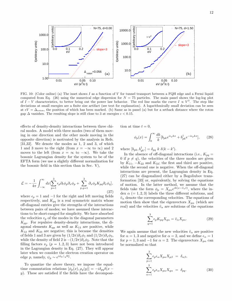
In Fig. 10, we show the I−V characteristics computedfor a system of N = 75 particles. Log-log plots in thesepanels show several plateaus and steps in the low voltageregion, which are purely due to the finite size effect ofsumming over a discrete set of spectral weights (in thelow-energy regime we have very few states in spite of thefairly large number of particles considered). We observe,surprisingly in view of the physics described in the in-troduction, that the exponent α in I ∼ V α remains veryclose to the ideal EFTA result of 3, within numerical er-rors. To explore the reasons behind the robustness of theedge exponent to nonlinearities in the dispersion, we haveplotted the energy at the maxima of the spectral func-tion A(k, ε) as a function of k in panel (d) of Fig. 9. Inthe energy region of interest (ε ≤ 0.2), the peaks roughlyfollow the ideal EFTA line. The low-energy states nearthe lower edge of the dispersion have comparatively lessspectral weight, and their contribution to the tunnelingdensity of states is negligible.

111

0 0.5 1

0.0

0.1

0.2

0.3

0.4

0.5

(a)

kl

E (

e2 /ε l)

0.00

1.69

3.38

5.06

6.75N=36, d=0.00

0 0.1 0.2 0.3 0.4 0.50

5

10

15

20

25

30

35

Ak (

arbi

trar

y un

its)

E (e2/ε l)

(b)

N=36, d=0.00kl=0.35 0.55 0.83 1.04 1.31

0 0.1 0.2 0.3 0.4 0.5 0.60

1

2

3

4

5

6

7

E(e2/ε l)

Spe

ctra

l Wei

ght

(c)

N=36, d=0.00

Single Boson2 Bosons3 Bosons4 Bosons5 Bosons6 Bosons7 Bosons>8 Bosons

0 0.5 1 1.50

0.1

0.2

0.3

0.4

0.5

0.6

(d)

kl

E (

e2 /ε l)

N=36 d=0.00

Nonlinear dispersionEFTA

FIG. 9: (Color online) (a) Bosonic spectra generated through electronic dispersion for N = 36 particles and d = 0.0 usingthe hybrid approach described in Sec. V.D; the bosonic spectral weights are shown in graduated colors. (b) Spectral functioncalculated from Eq. (22) for different k using the data in panel (a). (c) Bosonic spectral weights plotted as a function of theenergy, grouped by the number of bosons. (d) Energy at the maxima of the spectral function for different k. The black emptysquares indicate the situation for a linear dispersion corresponding to EFTA. The system has N = 36 particles; the setbackdistance is d = 0.0; and we have restricted to angular momentum up to ∆Mmax = 19.

B. Irrelevance of edge roton in tunneling

One might ask whether the edge roton produces anysignature in a tunneling experiment. In panel (a) of Fig.10, no significant structure is seen when eV is equal to theroton energy. Panel (b) corresponds to the setback dis-tance where the roton gap just vanishes. Again, there isno prominently visible structure that may be attributedto the roton energy. An increase in the density of statesat very low energies, shown in the log-log plots, is associ-ated with the edge roton, but such a signature would bedifficult to detect in experiments. We surmise that thespectral weight in the roton mode is too small for it tobe observable in tunnel transport.

VII. EFFECTIVE APPROACH FORRECONSTRUCTED EDGE AND TUNNELING

EXPONENT

For systems which undergo edge reconstruction (in ourcase d > dc), a logical procedure would be to study theexcitations around the new ground state which now oc-curs at a finite ∆M . This, however, is not possible in ournumerical calculations because of computational limita-tions. For example, in the 27 or 45 particle system, wecannot go to large enough values of ∆M to identify theminimum energy.

To make further progress, we make the assumptionthat the edge-reconstructed system can be described bymultiple chiral edges (we take three chiral edges below),which interact with one another. For want of a betterdescription, we further assume that each chiral edge canbe modeled by the EFTA Lagrangian and ask to whatextent this can describe the experiments.

We will use the technique of bosonization to study the

121

0.01 0.05 0.10 1.00

10.0

100.0

1000.0

eV (e2/ε l)

I(ar

bitr

ary

units

)

← slope=3

↓

∆ roton

=0.056

N=75, d=0.00

0.0 0.1 0.2eV

I(ar

bitr

ary

units

)

0.01 0.05 0.10

10.0

100.0

1000.0

10000.0

eV (e2/ε l)

I(ar

bitr

ary

units

)

← slope=3

N=75, d=1.50

0.0 0.1 0.2eV

I(ar

bitr

ary

units

)

I~V3

(a) (b)

FIG. 10: (Color online) (a) The inset shows I as a function of V for tunnel transport between a FQH edge and a Fermi liquidcomputed from Eq. (26) using the numerical edge dispersion for N = 75 particles. The main panel shows the log-log plotof I − V characteristics, to better bring out the power law behavior. The red line marks the curve I ∝ V 3. The step likedeviations at small energies are a finite size artifact (see text for explanation). A logarithmically small deviation can be seenat eV = ∆roton, the position of which has been marked. (b) Same as in panel (a) but for a setback distance where the rotongap ∆ vanishes. The resulting slope is still close to 3 at energies ε < 0.15.

effects of density-density interactions between three chi-ral modes. A model with three modes (two of them mov-ing in one direction and the other mode moving in theopposite direction) is motivated by the analysis in Refs.[31,32]. We denote the modes as 1, 2 and 3, of which1 and 3 move to the right (from x = −∞ to ∞) and 2moves to the left (from x = ∞ to −∞). We take thebosonic Lagrangian density for the system to be of theEFTA form (we use a slightly different normalization forthe bosonic field in this section than in Sec. V),

L = − 1

4π

∫ ∞−∞

dx[

3∑p=1

εp∂tφp∂xφp +

3∑p,q=1

∂xφpKpq∂xφq],

(27)where εp = 1 and −1 for the right and left moving fieldsrespectively, and Kpq is a real symmetric matrix whoseoff-diagonal entries give the strengths of the interactionsbetween pairs of modes; we have assumed these interac-tions to be short-ranged for simplicity. We have absorbedthe velocities vp of the modes in the diagonal parametersKpp. For repulsive density-density interactions, the di-agonal elements Kpp as well as K13 are positive, whileK12 and K23 are negative; this is because the densitiesof fields 1 and 3 are given by (1/2π)∂xφ1 and (1/2π)∂xφ3,while the density of field 2 is −(1/2π)∂xφ2. Note that thefilling factors νp (p = 1, 2, 3) have not been introducedin the Lagrangian density in Eq. (27). They will appearlater when we consider the electron creation operator onedge p, namely, ψp ∼ eiφp/

√νp .

To quantize the above theory, we impose the equal-time commutation relations [φp(x), ρq(y)] = −iδpqδ(x −y). These are satisfied if the fields have the decomposi-

tion at time t = 0,

φp(x) =

∫ ∞0

dk

k[bpke

iεpkx + b†pke−iεpkx], (28)

where [bpk, b†qk′ ] = δpq k δ(k − k′).

In the absence of off-diagonal interactions (i.e., Kpq =0 if p 6= q), the velocities of the three modes are givenby K11, −K22 and K33; the first and third are positive,while the second one is negative. When the off-diagonalinteractions are present, the Lagrangian density in Eq.(27) can be diagonalized either by a Bogoliubov trans-formation [33] or, equivalently, by solving the equationsof motion. In the latter method, we assume that thefields take the form φp = Xpαe

ik(x−vαt), where the in-dex α (= 1, 2, 3) labels the three different solutions, andvα denote the corresponding velocities. The equations ofmotion then show that the eigenvectors Xpα (which arereal) and the velocities vα are solutions of the equations

3∑q=1

εpKpqXqα = vαXpα. (29)

We again assume that the new velocities vα are positivefor α = 1, 3 and negative for α = 2, and we define εα = 1for p = 1, 3 and −1 for α = 2. The eigenvectors Xpα canbe normalized so that

3∑p=1

εpεαXpαXpβ = δαβ ,

3∑α=1

εpεαXpαXqα = δpq. (30)

13

If bpk and bαk denote the original and new (Bogoliubovtransformed) bosonic annihilation operators, we find thatthese are related as

bαk =

3∑p=1

Xpα[1

2(1 + εpεα)bpk −

1

2(1− εpεα)b†pk],

bpk =

3∑α=1

Xpα[1

2(1 + εpεα)bαk +

1

2(1− εpεα)b†αk].

(31)

Using Eq. (30), we can verify that [bpk, bqk′ ] = 0 and

[bpk, b†qk′ ] = δpq k δ(k− k′) imply that [bαk, bβk′ ] = 0 and

[bαk, b†βk′ ] = δαβ k δ(k − k′), as desired.

Let us now consider the electron creation operator onone of the three edges, say, ψ1 ∼ eiφ1/

√ν1 , where we

have assumed that edge 1 is associated with the fillingfactor ν1. In the absence of the off-diagonal interactions,ψ1 has the scaling dimension 1/(2ν1). In the presenceof interactions, we find from Eq. (31) that the scalingdimension of ψ1 is given by

d1 =(X11)2 + (X12)2 + (X13)2

2ν1. (32)

Since the second equation in Eq. (30) with p = q = 1implies that (X11)2 − (X12)2 + (X13)2 = 1, the expres-sion in Eq. (32) is larger than 1/(2ν1) if X12 6= 0, i.e., ifthere is a non-zero interaction K12 between modes 1 and2. We thus see that interactions between two counter-propagating modes lead to an increase in the scaling di-mension of the electron operator; hence the exponent forthe two-point correlation function for electrons becomeslarger than 1/ν1. In particular, if an edge corresponds toa filling factor of 1/3 or less, the electron correlation ex-ponent on that edge will be larger than 3. Thus a modelwith multiple chiral modes in which counter-propagatingedges interact with each other has difficulty in explainingthe results of tunneling experiments [4–7] which measurean exponent of about 2.7.

Wan et al [13] and Joglekar et al [34] also studied thereconstruction of FQH edges at ν = 1/3 and showed thatthe presence of counter-propagating edges leads to a non-universal exponent. Yang [31] introduced an action whichhas cubic and quartic terms in bosonic fields and showedthat this leads to an exponent slightly larger than 3. Incontrast, we have considered a standard action which isquadratic in bosonic fields and have shown that inter-actions between counter-propagating modes necessarilyleads to an exponent larger than 3.

VIII. DISCUSSION AND CONCLUSIONS

We have investigated the influence of nonlinear disper-sion on the physics of the FQH edge at ν = 1/3. Ourapproach involves microscopic calculations of the edge

dispersion and the associated bosonic spectra, and theuse of spectral weights from the bosonic theory.

The conclusions of our work are as follows.

i. The edge dispersion is linear for energies below0.02− 0.04e2/εl (0.2meV to 0.4meV) depending onthe electron-background separation. For d < dc =1.5l, an edge magnetoroton is observed. The maxi-mum roton gap is ∆ ≈ 0.056(e2/εl) for zero setbackdistance.

ii. Edge reconstruction occurs beyond a criticalelectron-background separation dc ≈ 1.5l forsmooth edges of a ν = 1/3 system, in agreementwith the previous literature [13].

iii. A bosonic description of the edge excitation spec-trum is satisfactory. It requires the dispersion ofthe single boson excitation as an input.

iv. The spectral weights of the electronic dispersion,though individually different from that of predic-tions of the bosonic theory, obey the same sumrules for a given angular momentum (provided Λlevel mixing is neglected).

v. The tunneling exponent is surprisingly insensitiveto the nonlinearity in the edge boson dispersion.The peaks of the spectral function for differentmomenta roughly follow the linearity of the idealEFTA. The low-energy states have a small spectralweights and contribute negligibly to the tunneling.

vi. The roton has no significant contribution to thespectral function and hence to the tunneling den-sity of states. Only a logarithmically weak signa-ture of the roton may be observed in tunneling ex-periments.

vii. It is well known that the model assuming a singlechiral mode is not adequate for understanding theresults of experiments on systems which undergoedge reconstruction. An effective theory descrip-tion with three chiral edges at ν = 1/3 producesan exponent that is larger than 3, contrary to theexperimental finding of a smaller-than-3 exponent.

IX. ACKNOWLEDGMENTS

We acknowledge Paul Lammert, Chuntai Shi, SreejithGanesh Jaya, and Vikas Argod for insightful discussions,support with numerical codes and cluster computing.The computational work was done on the LION-XC/XOand Hammer cluster of the High Performance Computing(HPC) group, The Pennsylvania State University.

14

X. APPENDIX

A. Sum rules

The derivation of the sum rules in Eq. (20) for squaredspectral weights at a given angular momenta

∑nl lnl =

M is given below. Consider the multinomial expansion(Ref. [18] p. 823)( ∞∑

k=1

xktk

k

)m= m!

∞∑n=m

∑aj

tn

n!

n!∏i x

aii∏

j(aj !jaj )

,

∑j

jaj = n, (33)

With the following transformations

m → b number of bosons,

xk → m inverse filling factor,

aj → nj bosons occupation,

n →M angular momentum,

we obtain( ∞∑k=1

mtk

k

)b= b!

∞∑M=b

∑nj

tM

M !

M !∏im

ni∏j(nj !j

nj ),

∑j

jnj = M. (34)

Hence we get

∞∑b=0

(1

b!

∞∑k=1

mtk

k

)b=

∞∑b=0

∞∑M=b

∑nj

tM∏j

mni

nj !jnj(35)

We simplify this by noting the relation

exp

(m

∞∑k=1

tk

k

)= e−m ln(1−t) =

1

(1− t)m. (36)

The sum of the squared spectral weights [9] is the coeffi-cient of tM∑

nl

|C(m)nl|

2 =(M +m− 1)!

M !(m− 1)!,∑l

lnl = M. (37)

B. Green’s function

The ideal EFTA assumes a linear dispersion ε(k) =vF k, and the sum rule in Eq. (37). The Green’s function

for the 1D chiral edge is

G(x, t) = 〈0|T (Ψ(x, t)Ψ†(0, 0))|0〉= 〈0|e−iHteik0Ψ(0, 0)e−ikxeiHtΨ†(0, 0)|0〉, t > 0.

(38)We map the edge to a disk by setting x = Rθ with radiusR = 1 and insert a complete set of states within thesubspace of single boson modes:

∑M

∑nl

|M, nl〉〈M, nl| = Is; M =∑l

lnl. (39)

We make the following substitutions

k = λM ; λ = M/√

6(N − 1)

εnl =∑l

εlnl = λvF∑l

lnl = λvFM, (40)

and proceed to calculate the Green’s function:

G(x, t) =∑M

∑nl

e−ikx〈0|Ψ(0, 0)eiHt|M, nl〉

×〈M, nl|Ψ†(0, 0)|0〉=∑M

∑nl

e−iλM(x−vF t)〈M, nl|Ψ†(0, 0)|0〉|2

=∑M

e−iλM(x−vF t)∑nl

|〈M, nl|Ψ†(0, 0)|0〉|2

=∑M

e−iλM(x−vF t)(M +m− 1

m− 1

)∼ 1

(x− vF t)m. (41)

This shows how the power law follows from a combina-tion of the linear dispersion and the sum rule. For ageneral dispersion ωk, we evaluate the commutators ofthe bosonic fields to find the Green’s function for theedge:

G(x, t) =2π

Lem

∑k

1k e−i(kx−ωkt)e−ak . (42)

1 D. C. Tsui, H. L. Stormer, and A. C. Gossard, Phys. Rev.Lett. 48, 1559 (1982).

2 X. G. Wen, Int. J. Mod. Phys. B 6, 1711 (1993).

15

3 X. G. Wen, Phys. Rev. Lett. 64, 2206 (1990).4 A. M. Chang, L. N. Pfeiffer, and K. W. West, Phys. Rev.

Lett. 77, 2538 (1996).5 M. Grayson, D. C. Tsui, L. N. Pfeiffer, K. W. West, and

A. M. Chang, Phys. Rev. Lett. 80, 1062 (1998).6 A. M. Chang, M. K. Wu, C. C. Chi, L. N. Pfeiffer, and K.

W. West, Phys. Rev. Lett. 86, 143 (2001).7 A. M. Chang, Rev. Mod. Phys. 75, 1449 (2003); M.

Grayson, Solid State Commun. 140, 66 (2006).8 S. S. Mandal and J. K. Jain, Solid State Communication118, 503 (2001); Phys. Rev. Lett. 89, 096801 (2002).

9 J. J. Palacios and A. H. MacDonald, Phys. Rev. Lett. 76,118 (1996).

10 F. D. M Haldane, Phys. Rev. Lett. 51, 605 (1983).11 J. K. Jain, Composite Fermions (Cambridge University

Press, Cambridge, 2007).12 R.B. Laughlin, Phys. Rev. Lett.,50, 1395 (1983).13 X. Wan, E. H. Rezayi, and K. Yang, Phys. Rev. B 68,

125307 (2003); X. Wan, K. Yang, and E. H. Rezayi, Phys.Rev. Lett. 88, 056802 (2002).

14 S. Jolad and J. K. Jain, Phys. Rev. Lett 102, 116801(2009).

15 U. Zulicke and A. H. MacDonald, Phys. Rev. B 54, R8349(1996).

16 A. Imambekov and L. I. Glazman, Science 323, 228 (2009).17 A. Imambekov and L. I. Glazman, Phys. Rev. Lett. 102,

126405 (2009).18 M. Abramowitz and I. A. Stegun, Handbook of Mathemat-

ical Functions (Dover, New York, 1972).

19 M. Grayson, M. Huber, M. Rother, W. Biberacher, W.Wegscheider, M. Bichler, and G. Abstreiter, Physica E 25,212 (2004).

20 O. Ciftja and C. Wexler, Phys. Rev. B 67, 075304 (2003).21 E. V. Tsiper, J. Math. Phys. 43, 1664 (2002).22 J. K. Jain, Phys. Rev. Lett. 63, 199 (1989).23 G. S. Jeon, C.-C. Chang, and J. K. Jain, Eur. Phys. J. B

55, 271 (2007).24 J. K. Jain and R. K. Kamilla, Int. J. Mod. Phys. B 11,

2621 (1997).25 G. Dev and J. K. Jain, Phys. Rev. B 45, 1223 (1992).26 J. K. Jain and T. Kawamura, Europhys. Lett. 29, 321

(1995).27 N. Metropolis, A. W. Rosenbluth, M. N. Rosenbluth, A.

M. Teller, and E. Teller, J. Chem. Phys. 21, 1087 (1953).28 W. K. Hastings, Biometrika 57, 1317 (1970)29 S. Chib and E. Greenberg, American Statistician 49, 327

(1995).30 For reviews, see: G. D. Mahan, Many Particle Physics,

third edition (Plenum, New York, 2000); G. F. Giulianiand G. Vignale, Quantum Theory of Electron Liquid (Cam-bridge University Press,Cambridge, 2005).

31 K. Yang, Phys. Rev. Lett 91, 036802 (2003).32 D. Orgad and O. Agam, Phys. Rev. Lett 100, 156802

(2008).33 C. Tsallis, J. Math. Phys. 19, 277 (1978).34 Y. N. Joglekar, H. K. Nguyen, and G. Murthy, Phys. Rev.

B 68, 035332 (2003).