Cutting-edge Relational Graph Data Management with Edge-k

Cutting-edge Relational Graph Data Management withEdge-k : From One to Multiple Edges in the Same Row

Lucas C. Scabora1, Paulo H. Oliveira1, Gabriel Spadon1, Daniel S. Kaster2,Jose F. Rodrigues-Jr1, Agma J. M. Traina1, Caetano Traina Junior1

1 University of São Paulo (USP), São Carlos, Brazil{luscascsb,pholiveira,spadon}@usp.br, {junio,agma,caetano}@icmc.usp.br

2 University of Londrina (UEL), Londrina, [email protected]

Abstract. Relational Database Management Systems (RDBMSs) are widely employed in several applications, in-cluding those that deal with data modeled as graphs. Existing solutions store every edge in a distinct row in the edgetable, however, for most cases, such modeling does not provide adequate performance. In this work, we propose Edge-k ,a technique to group the vertex neighborhood into a reduced number of rows in a table through additional columnsthat stores up to k edges per row. The technique provides a better table organization and reduces both table size andquery processing time. We evaluate Edge-k table management for insert, update, delete and bulkload operations, andcompare the query processing performance both with the conventional edge table — adopted by the existing frameworks— and with the Neo4j graph database. Experiments using Single-Source Shortest Path (SSSP) queries reveal that ournew proposal approach always outperforms the conventional edge table as well as it was faster than Neo4j for the firstiterations, being slightly slower than Neo4j only for iterations after having loaded the whole graph from disk to memory.It was able to reach a speedup of 66% over a representative real dataset, with an average reduction of up to 58% inour tests. The average speedup over synthetic datasets was up to 54%. Edge-k was also the best one when performinggraph degree distribution queries. Moreover, the Edge-k table obtained a processing time reduction of 70% for bulkloadoperations, despite having an overhead of 50% for individual insert, update and delete operations. Finally, Edge-kadvances the state of the art for graph data management within relational database systems.

Categories and Subject Descriptors: H.2.4 [Systems]: Relational databases; H.2.4 [Systems]: Query processing; H.2.1[Logical Design]: Schema and subschema; G.2.2 [Graph Theory]: Graph algorithms

Keywords: Graph Management, Query Processing, RDBMS

1. INTRODUCTION

Complex networks are employed to model data in several scenarios, such as communication infras-tructures, social networks, and urban street organization [Barabási and Pósfai 2016]. Those networksare commonly represented as graphs, in which nodes are mapped into vertices, and relationships intoedges. The number of applications using graph structures to represent data has increased significantly.Many of such applications seek to analyze the characteristics of graphs, employing algorithms such asPage Rank, as well as tackling problems such as finding the Single-Source Shortest Paths (SSSP) anddetermining the connected components of a graph [Silva et al. 2016].

Assume for example a graph representing authors and their publications, as illustrated in Figure 1.In this hypothetical graph, the relationship between two authors (e.g. Researchers A and B) is definedby their common publications, that is, coauthoring the same publication. Suppose that the weightw of the edge corresponding to such relationship is determined as 1/np, where np is the number of

This research was supported by FAPESP (Sao Paulo Research Foundation grants #2016/17330-1, #2015/15392-7,#2017/08376-0 and #2016/17078-0), CAPES and CNPq.Copyright c©2018 Permission to copy without fee all or part of the material printed in JIDM is granted provided thatthe copies are not made or distributed for commercial advantage, and that notice is given that copying is by permissionof the Sociedade Brasileira de Computação.

Journal of Information and Data Management, Vol. 9, No. 1, June 2018, Pages 20–35.

Cutting-edge Relational Graph Data Management with Edge-k: From One to Multiple Edges in the Same Row · 21

publications common to both authors. Then, 0 ≤ w ≤ 1, and weights close to 0 represent strongerrelationships (stronger lines in Figure 1), whereas weights close to 1 represent weaker relationships(thinner lines). In this scenario, assume that one wants to analyze the collaborative network regardinga specific author seeking to identify their direct and indirect coauthors. This action corresponds tosetting the specific author as a starting point (Researcher A in Figure 1) and exploring their directneighbors (Researcher B), then the next level of neighbors (Researcher C), and so on. The SSSPalgorithm can be employed to expand the frontier of visited neighbors from a given starting point.

Researcher A

Direct coauthor Indirect coauthor

0 ≤ weight ≤ 1

0 strong relationship (short distance)

1 weak relationship (long distance)

Researcher C Researcher B

Fig. 1: Example of a collaborative graph representing authors and their publications.

Identifying the proximity between authors and coauthors would allow the analysis of a researcher’simpact on their research field. The analysis can consider the weights of the edges explored by theSSSP algorithm. In this case, a weight close to 0 means a short distance between authors, due to ahigh number of shared publications. On the other hand, a weight close to 1 means a long distancebetween authors, due to a small number of shared publications. Hence, by identifying the shortestpaths from one author to all the others in the graph, the SSSP algorithm is able to determine thestrongest connections in the author’s collaborative network.

The rapid growth of Web-based applications has led to an increasing volume of graph data [Corbelliniet al. 2017]. Such volume is large enough to not fit entirely into main memory, compelling applicationdevelopers to rely on disk-based approaches. Relational Database Management Systems (RDBMS)provide infrastructure to support graph data management, with some useful features such as storage,data buffering, indexing, and query optimizations. However, they demand additional support tohandle graphs. There are several frameworks proposed to manage graphs on top of RDBMSs. TheFEM (Frontier, Expand and Merge) framework [Gao et al. 2011; Gao et al. 2014], for instance, wasproposed to translate analytical graph queries into Structured Query Language (SQL) commands.The implementation of FEM for SSSP queries consists of tracking frontier vertices and iterativelyexpanding them, merging the new elements with the set of previously visited ones.

The Grail framework [Fan et al. 2015], as well as its adaptation to the RDBMS Vertica [Jindal et al.2015], follows a similar approach, detailing query execution plans and allowing query optimizations.However, both frameworks are limited to a single graph modeling, and does not take into account thequery execution performance in alternative modelings. Both FEM and Grail frameworks employ onetable for the set of edges and another for the set of vertices. The edges are organized as a list, whereeach edge is stored as one row in the edge table. This representation determines the number of rowsrequired to store a vertex as one row for the vertex itself plus one row per edge, totaling the vertexdegree (i.e. number of neighbors) + 1.

In this paper, we propose Edge-k , a novel approach to model graphs in an RDBMS. The idea isto store the adjacencies of each vertex using an adjacency list that spans to multiple rows, with apredefined number k of edges per row. Our objective is to avoid tables with either too many rows ortoo many columns. A reduction in the number of rows decreases the required number of data blocks,which, in turn, reduces the space dedicated to row headers and the number of I/O operations. Areduction in the number of columns contrasts with storing the entire adjacency list in a single rowwhere the number of columns must be equal to the degree of the vertex with the maximum degreein the graph, which may not be known beforehand and may be unnecessarily large for other vertices.

Journal of Information and Data Management, Vol. 9, No. 1, June 2018.

22 · L. C. Scabora,P. H. Oliveira,G. Spadon, D. S. Kaster,J. F. Rodrigues-Jr,A. J. M. Traina and C. Traina-Jr

Moreover, by storing adjacencies in the same row, Edge-k ensures that at least part of them will becontiguously stored in the disk, which can further contribute to improve query performance.

Edge-k was initially proposed in [Scabora et al. 2017], where Edge-k was evaluated executing theSSSP procedure. The experiments were evaluated over both real and synthetic datasets, in orderto analyze the performance of SSSP query in an open-source RDBMS enhanced with Edge-k . Thereal dataset correspond to the author collaborations obtained from the Digital Bibliography & LibraryProject1 (DBLP), and the SSSP procedure ran for 2 to 5 iterations. Considering the synthetic datasets,on the other hand, SSSP ran until its completion, which required 4 iterations. We focused on theSSSP problem due to its major importance for numerous applications, such as to discover indirectrelationships in a social network and to find shortest paths to interesting tourist attractions. Theresults revealed a strong correlation between the average query execution time and the number of datablocks used to store the graph. Thus, reducing the number of blocks, which is related to reducing thenumber of rows and null values, leads to higher performance in queries.

In this paper, we extend our previous work exploring the Edge-k behavior when performing threeadditional analyses, described as follows.

� Insert, update, and delete operations. In addition to the data retrieval performance, weevaluate the performance of Edge-k in data maintenance operations. Although our approach bringsa minor overhead compared to the competitors, these operations tend to be less frequent than queryexecutions. Therefore, the overall impact of the Edge-k table tends to be minimal;� Bulkload operations. We developed a new technique, executed in the three steps Sort, Cast, andLoad, to perform the bulkload operation in Edge-k , where we achieved 70% of performance gainwhen compared to the bulkload operation over an ordinary edge table;� A more extensive evaluation of data retrieval. Along with the SSSP queries, we evaluate theperformance of Edge-k to retrieve the graph degree distribution. We also compared Edge-k bothwith the approach commonly employed in RDBMS and with the NoSQL graph database Neo4j. Theresults show the higher performance of our proposal against the evaluated competitors, allowing areduction of up to 66% of query processing time at the second iteration of the SSSP procedure,compared to the ordinary edge table over the DBLP dataset, and 58% in the first four iterations.

The remainder of this paper is organized as follows. Section 2 describes the background and relatedwork, covering the existing approaches for graph data management employing RDBMS. Section 3details the proposed Edge-k storage approach, including its extensions. In Section 4, we present theexperimental analyses and discuss the results. Finally, Section 5 concludes the work.

2. BACKGROUND AND RELATED WORK

Graph Definitions. A graph is represented as a pair G = {V,E}, where V is a set of verticesand E is a set of edges connecting vertices. A path p = v0

p; vn in a graph is a sequence of non-

repeated edges, in which there is one source vertex v0 and one target vertex vn. The weight of a pathis determined by the sum of the weights of its constituent edges. The Single-Source Shortest Path(SSSP) problem consists of finding the shortest path from a source vertex v0 to each vertex vi ∈ V ,that is, all paths v0

p; vi of minimum length. An algorithm that solves the SSSP problem is the

Bellman-Ford algorithm [Cormen et al. 2009], used in both FEM and Grail frameworks.

Graph Storage in RDBMSs. Our proposal is based on using the Relational Model to store andretrieve graphs. In this context, edges and vertex are stored as two distinct tables in an RDBMS,one for the vertices and other for the edges. Each vertex in V has a unique identifier attribute (id)

1http://dblp.uni-trier.de/



and may have as many attributes as needed for its properties. Considering the graph composed ofauthors and their articles, the properties are the details about authors and their articles. An edge inE is defined as an ordered pair 〈s, t〉, where s is the source vertex id and t is the target vertex id.Additional properties from each edge are stored in extra attributes of the relation, allowing detailingthe relationships among the vertices. A common property is the edge weight wi of each relationshipbetween s and t vertices. In this case, an edge will be defined as 〈s, t, w1, . . . , wj〉, where j is thenumber of properties of each edge. Figure 2 illustrates the vertex and edge tables that store the graphpresented in Figure 1, where each vertex has only one property: its name; and each edge has only oneproperty: the number of articles that both authors produced together.

s t w

A B 0.3

A C 0.2

A D 0.1

C D 0.5

... ... ...

Edge tableResearcher A

Researcher B

Researcher C

Researcher D

Vertex table

id name

A Researcher A

B Researcher B

C Researcher C

D Researcher D

... ...

Fig. 2: Example of Graph Storage in RDBMSs considering the author-relationship graph example in Figure 1.

There are three main approaches to store vertex or edges properties using RDBMS [Levandoski andMokbel 2009; Albahli and Melton 2016]: (i) triple store schema; (ii) binary tables; and, (iii) n-arytables. The triple store schema organizes vertices and edges into a triple <subject, property, object>,in which subject refers to the identifier of a vertex or an edge (e.g. the respective id attribute), propertydefines the attribute of the subject, and object is the property value. Following the entity-relationshipmodel, every attribute of both vertices and edges are represented as properties in the triple storeschema [Neumann and Weikum 2010]. Its major drawback derives from the object fields originatedfrom distinct properties, since they may have different data types. The binary tables storage schemagroups each distinct property into a specific table. As a result, each table has only two columns (henceit is named binary table): the entity identifier and its respective property value [Abadi et al. 2007].The third schema, i.e. the n-ary tables, includes the several properties as additional columns in thesame table. A special case of the n-ary table assigns all properties to the same table, which results ina property table [Levandoski and Mokbel 2009].

The main problem of the property table approach (i.e., the complete n-ary table) is the data sparsitycaused by heterogeneity in the entity set. DB2RDF [Bornea et al. 2013] was proposed to overcome thisdrawback, aggregating sets of properties into a single column. DB2RDF defines a maximum numberof properties for each row in the vertex table, where each property is represented by a pair of columnsdenoting its type and the respective value. A hash function will determine which property will beassigned to which column. Moreover, if a property needs to be stored in a column already filled, a newrow is inserted in the vertex table to accommodate this new property. The focus of DB2RDF is toreduce the space required to store the dataset since it stores distinct properties in a reduced numberof columns. However, DB2RDF focus on only associating vertices with their properties, not dealingwith the relationships among vertices and, consequently, with the shortest paths connecting them.

Graph Storage in Non-relational DBMSs. Due to storage problems in Web-based applica-tions, many companies investigate non-relational forms of storing data, resulting in NoSQL alter-natives [Corbellini et al. 2017]. NoSQL databases usually hold semi-structured and/or unstructureddata, mainly focusing on distributing the data storage and aiming at reducing complex join operations.Graph-oriented NoSQL databases store data in a graph-like structure, in which data are representedby vertices and edges. An example of such databases is the Neo4j2, an open source project based

2https://neo4j.com/



on Lucene indexes to store and access data from vertices and their relationships. The graph datastored in Neo4j are accessed through the Cypher or Gremlin languages, or are directly manipulatedvia a Java API. Studies revealed that Neo4j is more efficient than a relational database (MySQL)when dealing with traversal queries, i.e. queries looking for shortest paths with length bigger than3 [Vukotic et al. 2014; Vicknair et al. 2010]. However, it is important to mention that the performanceof Neo4j is negatively impacted by the size of the query result, which can achieve huge sizes for largergraphs and lengths [Vukotic et al. 2014].

An extension of DB2RDF is the SQLGraph [Sun et al. 2015], which employs a similar approachon non-relational databases. SQLGraph focuses on storing the properties of an edge as a JSONobject, overcoming the limitation of a fixed maximum number of properties in a single row. Thegraph transversals and update operations are performed by mixing SQL and Gremlin programminglanguages. Since SQLGraph does not deal with relational databases (like DB2RDF), the authorscompared it with Neo4j and Titan NoSQL databases.

A graph representation that does not comply with the first normal form of the Relational Model storesthe complete adjacency lists of each vertex in a column of type array [Chen 2013]. In this approach,each row has the source vertex id and its respective neighborhood (i.e. its list of target vertex id) ina single table column. According to the authors, this representation is well suited for sparse graphssince it avoids null values. However, such proposal only deals with scenarios in which all vertices havea small degree. As a consequence, the authors did not explore scenarios in which the neighborhoodcolumn size is bigger than a data block size.

Considerations. Our proposed Edge-k table focuses on improving RDBMS-based graph process-ing systems. In other words, instead of employing an array type of any size, we group the neighborhoodof a vertex into the edge table according to a maximum of k distinct values. Since our proposal coversa specialization of an edge table, it differs from both DB2RDF and SQLGraph because they eitherfocus on the vertex table or manage multiple edge tables in the same structure. Thus, our approachgathers the main advantages of the existing approaches while it strictly follows the Relational Model.

3. THE EDGE-K TABLE ORGANIZATION

There are two main approaches to store the edges of a graph as an RDBMS table. The first is to storeone edge per row; the problem with this approach is the need to scan tables with too many tuples.The second approach is to store the complete adjacency list of each node as a row; the problem hereis that, each vertex has a different number of neighbors, thus the number of columns must be thelargest vertex degree of the graph, which often leads to a table with a very high number of null values(as usually few nodes have such number of vertex). In both cases, the access and processing times perrow are expensive; our proposal solves both problems, described as follows.

Given a directed graph, our method stores the vertices in a table, and the edges in an Edge-k table.The tuples of the Edge-k table represent the edges as an adjacency list, but limiting the numberof edges to a maximum of k entries per tuple. When a source vertex has more than k edges, theadjacency list is divided into several tuples of at most k edges, as shown in Figure 3. The columns ofthe Edge-k table represent the source vertex, each of its target vertices, and the properties (or weights)of each corresponding edge. Notice that there will be k columns for each additional edge property, anddistinct properties will not be stored in the same column. Formally, assuming that only one propertyis stored per edge, an Edge-k table is represented as Ek = {s, 〈t1, w1〉 , 〈t2, w2〉 , 〈t3, w3〉 , ..., 〈tk, wk〉},where wi is the property weight of an edge linking vertex s to vertex ti, and 1 ≤ i ≤ k.

Since our proposal stores subsets of the vertex neighborhood in the same row, it enables the re-duction of the storage space, the number of disk accesses and the query response time, avoiding theaforementioned problems. Figure 3 illustrates part of the Edge-k table for a graph with a source



vertex v0 and a neighborhood of size n > k. Each edge has a property w. The left table shows theconventional approach in RDBMSs, which stores only one edge per row. The right table is a Edge-ktable, which stores up to k edges originated from a single vertex at the same row. Notice that thisexample is defined over a directed graph. However, our proposal also works on undirected graphs byreplicating the edges, and inverting the target and the source vertex id.

v1v3

v02

1

34

8

vX s t w

v0 v1 3

v0 v2 2

... ... ...

v2 vX 5

... ... ...

neighbor = 1

Conventionals t1 w1 ... tk wk

v0 v1 3 ... v2 2

v0 v3 4 ... vX 1

... ... ... ... ... ...

v2 v1 0.5 ... null null

... ... ... ... ... ...

Edge-k

neighbor = 1 neighbor = k

5

v2

Fig. 3: Comparison between the conventional and proposed approaches.

Our method differs from former alternatives by using the number k of columns as a parameter, whichfosters reducing the number of null values. The efficiency of our proposal is related to the parameterk, which affects (i) the number of rows and (ii) the unoccupied space of the table (null values).Reducing both (i) and (ii) decreases the number of tuples to be stored, consequently improving thequery performance. Since there can be mismatches between the neighborhood size n and the chosenk value, it is necessary to define rules to manipulate edges in the Edge-k table, discussed as follows:

� n = k: The ideal case is when n and k are equal, where a single completely-occupied row containsthe whole vertex neighborhood (without any null values).� n < k: When n is smaller than k, all the corresponding neighborhood fits in a single row and theremaining values are filled with null values. In Figure 3 this can be observed for source vertex v2,which requires null values to complete its row.� n > k: For values of n larger than k, the neighborhood is stored in groups of size k. The last groupstores at most k neighbors (second case) and thus the row is completed with null values. This lastcase is illustrated in Figure 3 by the source vertex v0, which have neighborhood size n = 2k. Inthis example, the neighborhood is divided into two complete rows (first case).

The details of our proposal are described as follows. Section 3.1 describes the equations used tomeasure the impact of the parameter k. Section 3.2 details how to manage an Edge-k table consideringinsert, update, delete and bulkload operations. Finally, Section 3.3 details how to adapt SSSP queriesto execute over an Edge-k table.

3.1 Estimation of the number of rows and of null values

In this section, we evaluate how to estimate the number of rows and null values that arise when usingthe Edge-k technique. The number of rows occupied by each source vertex v is defined as the smallestinteger greater than its total neighborhood size (degreev) divided by k. Therefore, the total numberof rows ηrows in the table is obtained as the summation of the number of rows for each v ∈ V , asexpressed in Equation 1.

ηrows =∑v∈V

⌈degreev

k

⌉(1)



The number of null values for each source vertex v is the number of remaining cells that were notfilled with target vertices data. This number is obtained computing how many target vertices are inthat row, which is the rest of the integer division of degreev by k. The number of columns filledwith null values for each vertex v is obtained by subtracting the number of target vertices previouslycalculated from k. A special case of this equation is when degreev = k, so the number of columnsfilled with null values is the rest of its division by k. The total number of null values is obtained bythe summation of the number of nulls for each v ∈ V , as is described in Equation 2.

ηnulls =∑v∈V

(k − (degreev mod k)) mod k (2)

The optimal scenario for Edge-k table is having every row fully filled for every source vertex. In thiscase, both the row overhead imposed by the row header (necessary to store internal control data, e.g.the 23 bytes of alignment padding) and the space lost by null values are minimum. However, such ascenario could only be achieved for the particular case in which every vertex has a fixed number ofneighbors. Unfortunately, this is not true for most graphs. For that reason, we use the metric exceedingto evaluate the impact of a given choice of k; it embodies the number of null values, redundant indexdata, and header data into a single number that indicates the cost of a k configuration. Equation 3computes the exceeding metric. Notice that the terms ηnulls and ηrows are both function of k.

exceeding = (ηnulls ∗ null_size) + (ηrows − |Vneigh|) ∗ (size(vid) + overhead) (3)

where Vneigh ⊆ V is the subset of vertices containing a neighborhood; size(vid), overhead andnull_size are the sizes in bytes respectively of the vertex id, of the row overhead and of the storageof a null target. The first part of Equation 3 computes the space occupied by null values given by theproduct of ηnulls and of the space occupied by each null value (null_size). The second part considersthe wasted space occupied by replicating source vertices vid, which occurs whenever the neighborhoodsize is greater than the chosen k value. In other words, ηrows − |Vneigh| corresponds to the numberof extra rows in an Edge-k table, which is multiplied by the cost of each additional row. The costof every additional row is defined by the replicated source vertex vid plus the row overhead. Finally,Equation 3 sums these two parts to determine the total exceeding space.

The value of null_size depends on how the RDBMS implements null values. When it does notcompact null values, it is the standard size in bytes of the corresponding attribute. In this case,null_size = size(vid). However, an RDBMS usually applies techniques to save space when storingnull values, and the real size varies according to the product. Although Equations 1 to 3 help users totune the storage of graphs for every scenario, our proposal depends on choosing an informed value fork to allow better results. In our experiments, we explored various values of k, analyzing their impacton the Edge-k table and on the query processing time (see Section 4.2).

3.2 Edge-k Table Management

This section details how to manage an Edge-k table considering the operations of insert, updateand delete edges. Executing those operations over an Edge-k table is more expensive than over aconventional table because they demand not only locating a row, but also finding its respective column(target vertex) in that row. Each operation is implemented as a procedure, detailed as follows.

To execute an edge insert operation, it is required to search for an empty spot in the rows of Edge-ktable already storing edges from the same source vertex. If an available spot exists, the correspondingtarget vertex will be written to the last row of the source vertex along with its properties, creating anew target vertex, and its associated properties. Otherwise, a new row will be created, inserting the



new edge and filling up the remaining spots with null values. For the update operation, the approachis similar, however searching for the column pointing to a specific target vertex and updating itsproperty values. Here, we assume that the update operation refers solely to changing some propertyof a given edge, such as the weight value. Updating the source or target vertex is equivalent to adeletion followed by the creation of a new edge.

The delete operation is more complex. It always tries to maximize the number of complete rows,that is, maintain rows without any null values. For example, consider the deletion of an edge betweensource vertex vs and target vertex vt. This edge will be deleted by assigning null to the columncorresponding to vt in a row r. There are two cases: (i) Either row r is incomplete or all rows ofvertex vs are complete. In this case, we just swap the value in the column of vertex vt with the valuefrom the last occupied column in the same row; (ii) There is an incomplete row r’. In this case, theswap operation occurs between r and r’, replacing the last occupied column in row r’ with the valuefrom the column corresponding to vt in row r. Afterward, the columns corresponding to vt and theirrespective properties are filled with null values. If such operation removes the last target vertex inthe row, this row is removed from the table.

We also developed a bulkload operation for the Edge-k table. This operation receives as input acomma-separated file (i.e. a CSV file, containing each edge in a distinct row, as shown in Figure 2)and is executed in three steps: Sort: a disk-based sort operation over the lines of the CSV file basedon the source vertex id ; Cast: convert the sorted file, with one edge per line, into another CSV filecontaining k edges per line; and Load: execute the bulkload in the RDBMS using the converted file.The sorting step is required because, in the second step, we sequentially read the CSV file lines andcombine them in the same row as long as the source vertex remains the same.

3.3 Adaptation of Single-Source Shortest Path (SSSP) procedure

The SSSP query is a search-find greedy-based algorithm. It starts at a user-given location (i.e. thesource vertex), from which it will iteratively expand the vertex’s neighborhood (or frontier) until itreaches a given stop criterion. The SSSP algorithm can run: (a) until it calculates the distances to allthe vertices of the network; (b) until it finds the desired destination; or (c) until it completes a certainnumber of iterations. The three cases are achieved through the process of vertex expansion, whichimplies in searching the neighborhood of another vertex that pertains to the current vertex, suchthat, at each iteration, the neighborhood of a new vertex will be searched, which becomes the newcurrent source vertex. To perform the SSSP algorithm on a Edge-k table, we adapted the procedurecommonly employed in the literature. Algorithm 1 describes the SSSP query using our proposal, andFigure 4 illustrates its execution.

id dist prev

v0 0 -1

s t1 w1 ... tk wk

v0 v1 3 ... v2 2

v0 v3 4 ... vX 1

v2 v1 0.5 ... null null

... ... ... ... ... ...

Edge-kStart

id dist prev

v0 0 -1

... ... ...

result

did it change?

Yes

No

End

id dist prev

v0 0 -1

v1 3 v0

v2 2 v0

... ... ...

newResult

Initializeresult table

=next

iteration

Fig. 4: Illustration of the SSSP procedure adapted to our proposal.

Initially the SSSP procedure creates a temporary table, called result, intended to register all thevisited vertices. The result table keeps track of the unique identifier (id) of each vertex, its minimumdistance to the source vertex (dist), and the previous vertex (prev) in the respective shortest path,allowing the identification of the edges that compose such path. This initial step inserts the sourcevertex v0 into result, with a distance of 0 and no previous vertex (i.e. -1). This step is represented



in the leftmost part of Figure 4. Step 1 corresponds to Lines 2–4 of Algorithm 1, which initializes thecontinue flag, the currentIteration counter, and the result table.

Thereafter, the procedure performs a while loop (Lines 5–11 of Algorithm 1), depicted in Figure 4as the operations within the gray box and the condition evaluation at the right. In Line 5, the loopchecks whether the continue flag is active, as well as compares the currentIteration counter to themaximum number of iterations provided by the user. If both conditions are met, result is joined withthe Edge-k table, expanding the frontier of visited vertices and updating the distance of the shortestpath to each target vertex. This step produces a new temporary table, called newResult (Line 6). Toupdate the distance of a path, our procedure sums the accumulated distance (dist in result) and thedistance wi (stored in the Edge-k table) to the next neighboring vertex ti, where 1 ≤ i ≤ k. Regardingthe example in Figure 4 (corresponding to the graph of Figure 3), after the first iteration, the weightsof paths v0

p; v1 and v0

p; v2 are, respectively, (0 + 3) and (0 + 2). Our procedure seeks to minimize

such weights, keeping the minimum paths found so far. Therefore, in the second iteration, when theprocedure visits vertex v2, the weight of path v0

p; v1 is updated to 2.5.

Then, in Line 7, the procedure checks whether the contents of result and newResult tables are thesame, counting the number of distinct rows and storing it in the continue flag. That is, if the contentsare equal, then continue equals 0. In this case, when the procedure checks the loop conditions again(Line 5), the loop will be over, finishing the SSSP execution. After updating the continue flag, theprocedure drops the result table, makes newResult the up-to-date result table, and incrementscurrentIteration (Lines 8–10). Then, another iteration begins.

Algorithm 1 Execution of SSSP in Edge-k1: function SSSP(Edge-k, sourceVertex, maxIterations)2: continue ← 13: currentIteration ← 04: Create and Initialize result table with sourceVertex5: while (continue > 0) AND (currentIteration < maxIterations) do6: Visit neighbors of current node by joining tables result and Edge-k, resulting in a new table named newResult7: Do a NATURAL FULL JOIN between result and newResult to check whether their contents are the same, counting

the number of distinct rows and storing it in continue8: Drop table result9: Rename newResult to result

10: currentIteration ← currentIteration + 111: end while12: end function

The main difference of Edge-k compared to other proposals is the join of the temporary resulttable with the edge table. In the existing frameworks, the edge table stores only one target vertexper row. Therefore, when joining the result and edge tables, the other procedures just performs anordinary JOIN operation. Conversely, in Edge-k , for any value of k, such JOIN operation features anunnesting step, which consists of mapping the multiple t1 . . . tk columns from the Edge-k table intoseparate rows. Accordingly, Edge-k allows executing JOIN operations for any value of k.

4. EXPERIMENTAL RESULTS

4.1 Setup

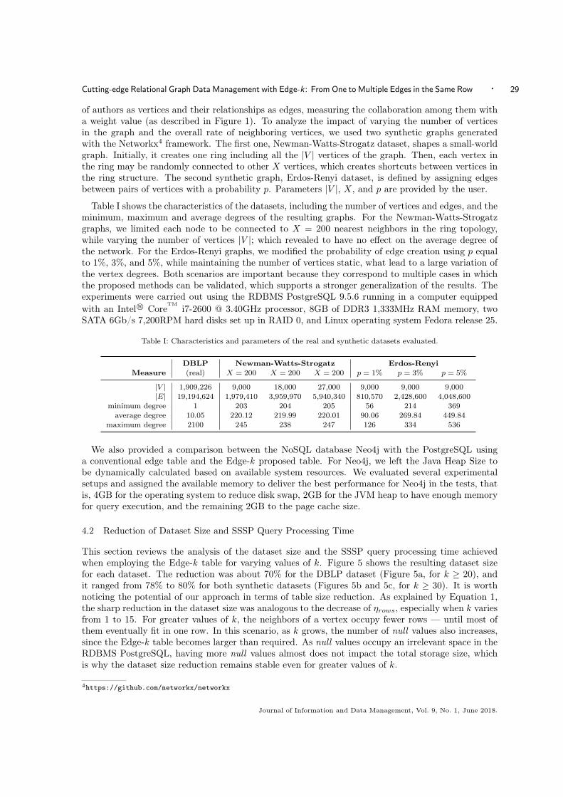
We evaluated our proposal on both real and synthetic datasets, and we present here the resultson representative datasets. The real dataset was extracted from the Digital Bibliography & LibraryProject3 (DBLP), containing information about authors and their publications. We modeled the set

3Dataset from March 16, 2017 — available at http://dblp.uni-trier.de/xml/



of authors as vertices and their relationships as edges, measuring the collaboration among them witha weight value (as described in Figure 1). To analyze the impact of varying the number of verticesin the graph and the overall rate of neighboring vertices, we used two synthetic graphs generatedwith the Networkx4 framework. The first one, Newman-Watts-Strogatz dataset, shapes a small-worldgraph. Initially, it creates one ring including all the |V | vertices of the graph. Then, each vertex inthe ring may be randomly connected to other X vertices, which creates shortcuts between vertices inthe ring structure. The second synthetic graph, Erdos-Renyi dataset, is defined by assigning edgesbetween pairs of vertices with a probability p. Parameters |V |, X, and p are provided by the user.

Table I shows the characteristics of the datasets, including the number of vertices and edges, and theminimum, maximum and average degrees of the resulting graphs. For the Newman-Watts-Strogatzgraphs, we limited each node to be connected to X = 200 nearest neighbors in the ring topology,while varying the number of vertices |V |; which revealed to have no effect on the average degree ofthe network. For the Erdos-Renyi graphs, we modified the probability of edge creation using p equalto 1%, 3%, and 5%, while maintaining the number of vertices static, what lead to a large variation ofthe vertex degrees. Both scenarios are important because they correspond to multiple cases in whichthe proposed methods can be validated, which supports a stronger generalization of the results. Theexperiments were carried out using the RDBMS PostgreSQL 9.5.6 running in a computer equippedwith an Intel R© Core

TMi7-2600 @ 3.40GHz processor, 8GB of DDR3 1,333MHz RAM memory, two

SATA 6Gb/s 7,200RPM hard disks set up in RAID 0, and Linux operating system Fedora release 25.

Table I: Characteristics and parameters of the real and synthetic datasets evaluated.

DBLP Newman-Watts-Strogatz Erdos-RenyiMeasure (real) X = 200 X = 200 X = 200 p = 1% p = 3% p = 5%

|V | 1,909,226 9,000 18,000 27,000 9,000 9,000 9,000|E| 19,194,624 1,979,410 3,959,970 5,940,340 810,570 2,428,600 4,048,600

minimum degree 1 203 204 205 56 214 369average degree 10.05 220.12 219.99 220.01 90.06 269.84 449.84

maximum degree 2100 245 238 247 126 334 536

We also provided a comparison between the NoSQL database Neo4j with the PostgreSQL usinga conventional edge table and the Edge-k proposed table. For Neo4j, we left the Java Heap Size tobe dynamically calculated based on available system resources. We evaluated several experimentalsetups and assigned the available memory to deliver the best performance for Neo4j in the tests, thatis, 4GB for the operating system to reduce disk swap, 2GB for the JVM heap to have enough memoryfor query execution, and the remaining 2GB to the page cache size.

4.2 Reduction of Dataset Size and SSSP Query Processing Time

This section reviews the analysis of the dataset size and the SSSP query processing time achievedwhen employing the Edge-k table for varying values of k. Figure 5 shows the resulting dataset sizefor each dataset. The reduction was about 70% for the DBLP dataset (Figure 5a, for k ≥ 20), andit ranged from 78% to 80% for both synthetic datasets (Figures 5b and 5c, for k ≥ 30). It is worthnoticing the potential of our approach in terms of table size reduction. As explained by Equation 1,the sharp reduction in the dataset size was analogous to the decrease of ηrows, especially when k variesfrom 1 to 15. For greater values of k, the neighbors of a vertex occupy fewer rows — until most ofthem eventually fit in one row. In this scenario, as k grows, the number of null values also increases,since the Edge-k table becomes larger than required. As null values occupy an irrelevant space in theRDBMS PostgreSQL, having more null values almost does not impact the total storage size, whichis why the dataset size reduction remains stable even for greater values of k.

4https://github.com/networkx/networkx



Regarding the SSSP query processing times over the Edge-k table, we defined a query whose startingpoint was the vertex having the highest degree — the largest number of neighbors. Each query wasperformed 30 times, and the average execution time was obtained by discarding 10% of the shortestand 10% of the largest results. For the DBLP dataset, we analyzed the average execution times from2 to 5 iterations of the SSSP algorithm — i.e. the number of times the tables Edge-k and result arejoined to compute shortest paths, as described in Section 3.3. For the synthetic datasets, a maximumof 4 iterations was enough to visit all the vertices. Therefore, we executed the complete SSSP querywithout limiting the number of iterations.

1 5 10 15 20 25 30 35 40 45 50Value of k

160

240

320

400

480

560

640

720

800

Edg

e ta

ble

size

(MB

)

Reduction stabilizes at 70%for k values greater than 20

(a) DBLP.

1 5 10 15 20 25 30 35 40 45 50Value of k

0275481

108135162189216243270

Edg

e ta

ble

size

(MB

)

Average reduction time rangesfrom 78% to 80% for k valuesgreater than 30

9,000 vertices18,000 vertices27,000 verticesaverage

(b) Newman-Watts-Strogatz.

1 5 10 15 20 25 30 35 40 45 50Value of k

0

18

36

54

72

90

108

126

144

Edg

e ta

ble

size

(MB

)

Same behavior of Figure (b)

p = 1%p = 3%

p = 5%average

(c) Erdos-Renyi.

Fig. 5: Size reduction, in megabytes, of the Edge-k table achieved in each evaluated dataset as k varies.

Figure 6 presents the average query-time to execute a SSSP query varying k when considering thesecond, third and fourth iterations for the DBLP graph (Figure 6a), for the Newman-Watts-Strogatzgraph (Figure 6b) and for the Erdos-Renyi graph (Figure 6c). The SSSP query processing time was notevaluated for the first iteration alone, since the same outcome could be obtained by simply queryingthe edge table, filtering it by the source vertex, rather than performing join operations. The queryprocessing time observed in Figure 6a achieved a maximum reduction of 66% at the 2nd iteration and,regarding the average values, a reduction of 58% when k u 18, while in Figure 6b this reduction variesfrom 50% to 54% when k = 10 and, in Figure 6c, the highest average reduction was about 52% atk = 30. Notice that the behavior presented over all datasets is analogous to the dataset size reduction.

1 5 10 15 20 25 30 35 40 45 50Value of k

0

10

20

30

40

50

60

70

80

Ave

rage

tim

e (s

)

Highest average reductionof 58% near k = 18

Max reduction achieved of 66%

Number of iterations2nd iteration3rd iteration

4th iterationaverage

(a) DBLP.

1 5 10 15 20 25 30 35 40 45 50Value of k

5

10

15

20

25

30

35

40

45

Ave

rage

tim

e (s

)

Average reductionbetween 50% and54% for k valuesgreater than 10

Number of vertices 9,000 vertices18,000 vertices27,000 verticesaverage


1 5 10 15 20 25 30 35 40 45 50Value of k

0

3

6

9

12

15

18

21

24

Ave

rage

tim

e (s

)

Highest average reductionof 52% at k = 30

Probability for edge creationp = 1%p = 3%

p = 5%average

(c) Erdos-Renyi.

Fig. 6: Average time to process a SSSP query in three scenarios for varying k in the Edge-k table: the DBLP datasetwith the second, third and fourth iterations, the Newman-Watts-Strogatz graph and the Erdos-Renyi graph.

Additional experiments, not presented in this paper, were performed for larger values of k. Wefound that beyond this point the average query time only increases. This is because the number ofnull values rises steadily. In other words, indefinitely increasing the k value also increases the numberof unnecessary columns in the Edge-k table, adding more validations to the unnesting operation (see



Algorithm 1). Thus, assigning a value too large for k negatively affects the SSSP query performance.However, the total number of unnecessary columns can be estimated through ηnulls (see Equation 2).

Finally, we also carried a scalability analysis to identify the highest reduction achieved in the SSSPquery processing time while varying: (i) the number of iterations performed over the DBLP graph;and (ii) the distinct parameter value used to generate the synthetic graphs. Figure 7 shows the largestreduction of the query processing time achieved over the DBLP dataset while varying number ofiterations. In Figure 7a, the largest reduction was achieved with 2 iterations, and as the numberof iterations increases, this reduction decreases. This implies that the query performance tends todegrade as the Edge-k and result tables are repeatedly joined. Nevertheless, solutions that employtoo many joins are not usually well-suited for an RDBMS, such as looking for collaborations that haveat least 5 authors. Considering our real dataset, performing more than 5 iterations means lookingfor collaboration paths between authors with lengths having at least 5 distinct authors. Such largelengths tend to be less frequent. Hence, it would not be particularly interesting to keep SSSP runningany further than the number of iterations for which it already ran.

2nd 3rd 4th 5th0

20

40

60

80

100

Red

uctio

n (%

)

66% 61%49% 43%

Number of iterations

(a) DBLP.

9,000 18,000 27,0000

20

40

60

80

100

Red

uctio

n (%

)

51.3% 55.7% 56.3%

Number of vertices


1% 3% 5%0

20

40

60

80

100

Red

uctio

n (%

)

47.6%55.5% 55.8%

Probability for edge creation

(c) Erdos-Renyi.

Fig. 7: The largest query processing time reductions, using the Edge-k method. (a) Varying the number of iterationsin the DBLP dataset; (b) Increasing numbers of vertices for Newman-Watts-Strogatz graph; and (c) Increasing thenumber of edges for Erdos-Renyi graph (see Table I).

Considering the synthetic datasets, increasing the number of vertices |V | in the Newman-Watts-Strogatz graph (Figure 7b) and the probability p of edge creation (Figure 7c) have provided betterprocessing times. Both Figures 7b and 7c show that our proposal provides even better results as thevolume of data grows. That is, graphs that would have more rows in a conventional edge table (and,consequently, a larger number of repeated source vertex in the conventional implementation) wouldallow a larger reduction in both query processing time and dataset size.

These experimental results show that it is possible to accomplish good performance improvementsregardless of the number of vertices and of resulting vertex degrees. Considering the number ofiterations performed by the SSSP procedure, the reduction in query processing time diminishes as thenumber of iterations increases. However, this is an issue already known in RDBMS-based solutionsinvolving too many join operations.

4.3 Table Management Analysis

This section summarizes two analyses; the overhead in individual insert, update, and delete operations;and the bulkload operation. Both analyses are performed over the DBLP dataset. Regarding the firstanalysis, since the most significant reductions in dataset size and SSSP query time occurred for kvarying from 1 to 15, we evaluated the overhead in the insert, update, and delete operations usingk = 1, 5, 10, and 15. Notice that k = 1 is a special case where the Edge-k table corresponds to aconventional edge table. We started by randomly generating 1,000 new edges, inserting all of theminto each one of the four tables; i.e. in the conventional edge table and in the Edge-k tables withk = 5, 10, and 15, respectively. Then, we updated the weight property of the new edges in every table.



Finally, we deleted the same 1,000 edges from each table. Figure 8 shows the average time and thestandard deviations, calculated based on the time to manipulate the 1,000 random edges, discarding10% of the shortest and 10% of the largest times.

Based on the times observed in Figure 8a, the overhead is about 50% for the insert, update, anddelete operations when using the Edge-k table with k 6= 1. That is, instead of executing each of thethree operations in 10 ms, they took approximately 15 ms. The elapsed times for k = 5, 10 or 15 werealmost the same, indicating that the overhead occurs mostly due to the search for the desired targetvertex. Since this search is performed in main memory — i.e. after loading the affected rows fromthe disk — the value of k does not pose a heavy impact on the processing time. However, there isan overlap among their standard deviations, especially in the insert operation. Nevertheless, most ofthe graph analyses are performed over static graphs, thus this overhead does not affect the final user.Even for dynamic data, many applications requires search operations more frequently than insert,update and delete operations. For those applications, our Edge-k method is better suited.

Insert Update Delete

0

5

10

15

20

25

30

Ave

rage

tim

e (m

s)

Around 15ms (50% overhead)

ConventionalEdge-k (k = 5)

Edge-k (k = 10)Edge-k (k = 15)

(a) General operations in an RDBMS.

1 5 10 20 30Value of K

0

50

100

150

200

Ave

rage

Tim

e (s

) Reduction of 35% when k = 2

Average reduction of 70%with k values greater than 10

SortCastLoad

(b) Bulkload average times per k value.

Fig. 8: (a) Average elapsed time of insert, update and delete operations in an RDBMS over a Edge-k table. (b)Average execution time of bulkload operations for varying k, which are performed following the three steps describedin Section 3.2: Sort, Cast, and Load.

For the bulkload analysis, we followed the three steps described in Section 3.2: Sort, Cast, andLoad. Figure 8b shows the average bulkload times as k varies from 1 to 30. Each measurement wascollected 20 times, discarding 10% of the shortest and 10% of the largest times. Notice that for theconventional edge table (i.e. k = 1) only the Load step is required, although it requires more timeto complete when compared to other values of k. By comparing the k values of 1 and 2, we observea reduction of 35%, even executing the Sort and Cast steps (required when k ≥ 2). As k increases,the time reduction stabilized around k = 10 with a reduction about 70% in total. The time reductionduring bulkload operations are mainly related to the sharp reduction in the ηrows (see Equation 1).

4.4 Comparison of Edge-k to the Conventional Edge Table and a NoSQL Graph Database

In this section, we compare Edge-k to the NoSQL graph database Neo4j, as well as to the conventionaledge table. Considering the sharp reduction in the SSSP query processing time, which occurs for kup to 15, as discussed in the last two sections, this comparison was performed using k = 10. Wealso compared with the conventional edge table. We implemented both graph degree distribution andSSSP queries in Neo4j using the Java API, aiming at comparing the same algorithm in both databases.

The degree distribution query counts the number of vertices for each possible degree (i.e. thenumber of neighbors of each vertex) in the graph. In Neo4j, this query was implemented performinga loop through all vertices counting the number of neighbors for each vertex. In PostgreSQL, thisquery is performed with the GROUP BY clause on the source vertex identifier, followed by the COUNTaggregate function on the number of associated target vertices. Considering the Edge-k table, thequery counts the number of target vertices in each row. The query finishes by summing the quantityof target vertices per row and employing the GROUP BY clause on the source vertex identifier. After



running the degree distribution query 30 times, and discarded 10% of the shortest and 10% of thelargest times, we computed the average time for each evaluated approach. The result was 3.17s forEdge-k , 6.21s for Neo4j, and 9.68s for the conventional edge table. This result is promising because,while Neo4j outperformed the conventional edge table, Edge-k outperformed both competitors.

We implemented the SSSP query on Neo4j using Algorithm 1, employing a HashMap structure forthe temporary table. This algorithm enables comparing the DBMS-based approaches explored in thiswork. In this analysis, we focused on the evaluation of distinct initial source vertices (i.e. querycenters) to compare Edge-k to Neo4j and to the conventional edge table. Such evaluation enabledanalyzing distinct behaviors in terms of processing time as the query centers vary. The processingtime changes because each source vertex can have either many or few connections, and being eithera vertex close or remote with respect to the other vertices. Accordingly, a remote vertex is likely todemand less iterations to reach a hub and, until that point is reached, the query processing time willbe low, since there will be fewer connected elements to be joined during the iterations of Algorithm 1.

Following that reasoning, we randomly chose twenty query centers, ten having vertex degree nearthe minimum vertex degree distribution, and ten having degree near the maximum degree distribution.For each query center, we calculated its SSSP varying the number of iterations from 1 to 15. At the 15thiteration, SSSP stopped for some query centers because their result table did not change anymore(see line 7 in Algorithm 1). Each iteration was computed three times, in order to minimize any queryprocessing time deviation. By grouping the twenty values based on their iteration number and sortingthese values, we got all values that were in the first, second, and third quartiles. Figures 9a–9c showthese values regarding Neo4j, the conventional edge table, and the Edge-k table, allowing us to analyzehow much processing time changed for varying degrees.

1 2 3 4 5 10 15Number of iterations

101

100

101

102

103

Tim

e (s

)

Quickly grows due to intensive readsfrom disk (list of visited neighbors)

Flattens when it loads mostof the graph data in memory

1st quartile

2nd quartile3rd quartile

(a) Neo4j processing time.


101

100

101

102

103

Tim

e (s

)

Times uniformly increasingas the join operation occurs

1st quartile


(b) Conventional processing time.


101

100

101

102

103

Tim

e (s

)

Same uniform growth asfor conventional table

1st quartile


(c) Edge-k processing time.


101

100

101

102

103

Ave

rage

tim

e (s

)

Neo4j is 10 times faster

Edge-k is always faster thanthe Conventional approach

Neo4j outperforms thecompetitors at the end,but it ties with Edge-k

Neo4jConventionalEdge-k

(d) Average time in all systems.

1 2 3 4 5 6 7 8Number of iterations

0.00.20.40.60.81.01.21.41.61.82.0

Num

ber o

f vis

ited

verti

ces

(x 1

06 )

1st quartile

2nd quartile (Median)3rd quartileAverage

(e) Number of visited vertices per iteration.

Fig. 9: Time comparison for the SSSP query on Neo4j, on conventional edge table, and on Edge-k table, as the initialsource vertex and the number of iterations vary. For each iteration, we also present the number of visited vertices.

For the three upper plots, the first quartile represents 25% of the elapsed time as the query center



varies, the second represents 50%, and the third represents 75%. Figure 9e shows the number of visitednodes per iteration considering the quartiles, including the respective average value. These resultsshow that, in all cases, the series converge toward the same elapsed time. This means that the timeis independent of the query center as the number of iterations increases. This behavior occurred forall evaluated techniques. The experiment evaluates the deviation from the median time of the threecases. We provided different perspectives to visualize the results, which reveal the inherent structureof the complex network representing the DBLP data. We showed that the results behave similarly forany query center, and also that our analysis is stable and that it can be generalized to any similarcomplex network, that is, to any free-scale network.

Additionally, Figure 9a shows that the execution times of Neo4j quickly grow for all quartiles.This is a consequence of intensive disk read operations, caused by the sharp increase in the visitedneighbors list size (see Figure 9e). We always cleaned the cache before each SSSP query executionand employed a centralized version of Neo4j, thus the database demands a large processing time tobring the accessed vertices to the main memory. Such finding was expected according to Section 2,which relates the performance of Neo4j with the query result size. However, after loading most ofthe graph in the main memory, each iteration takes a small time. Considering the conventional andEdge-k tables, the elapsed time of both approaches increase uniformly.

Finally, Figure 9d shows the average time for the twenty query centers comparing Neo4j, conven-tional edge table and Edge-k table. In the first iteration, Neo4j was 10 times faster, but in the nextiterations, it was negatively impacted by the visited neighbors list size, as previously discussed. Inthe 15th iteration, Neo4j outperformed the competitors, but with an execution time very similar toour proposal. Furthermore, the Edge-k table always outperformed the conventional edge table for anynumber of iterations greater than 1.

5. CONCLUSION

The RDBMSs have been challenged by the growing volume and complexity of graphs demanded andgenerated by recent applications. Therefore, an RDBMS provides the infrastructure to manipulatesuch data, but its efficiency depends on the graph representation. Despite the several ways to representgraph data in an RDBMS, most of the frameworks that process graph queries focus on a singleapproach to store the edges of a graph. In this context, we proposed the Edge-k table, an alternativestorage approach. It consists of representing the neighborhood of each vertex in a few or even in asingle row. To maintain the robustness and to keep compatibility to the Relational Model, we definedthat each group can store up to a predefined amount of k edges in a single row.

This work is based on the assumption that a Edge-k table can reduce the dataset size and, con-sequently, the processing time of queries. In fact, regarding query processing time, the experimentalresults over a real dataset showed a maximum of up to 66% at the second iteration of a SSSP query,as well as an average reduction of about 58% for the first four iterations. Regarding the two syntheticdatasets evaluated, we obtained an average reduction ranging from 50% to 54%. Those results high-light the positive impact of Edge-k when compared to existing RDBMS-based graph-data managementframeworks. We also performed three analyses to explore our method, described as follows.

� Insert, update, and delete operations. The overhead of a Edge-k table for such operationswas about 50%, increasing the execution times to around 15 ms. However, since such operationsusually are much less frequent than search operations, the overall impact of Edge-k is minimal;� Bulkload operations. We proposed an method to perform bulk insertions into the Edge-k tablethat executes three steps (i.e. Sort, Cast, and Load). In the corresponding analysis, we achieved atime reduction average of 70% when k ≥ 10, mainly due to the smaller number of affected rows;� A more extensive evaluation of data retrieval. Along with the SSSP queries, we evaluatedthe performance of Edge-k in a degree distribution query. Additionally, we compared Edge-k both



with the conventional edge table in an RDBMS and with a NoSQL graph database. Regardingthe vertex degree distribution query, Edge-k has outperformed both competitors. Considering theSSSP queries, Edge-k has outperformed Neo4j in most iterations (13 out of 15). Furthermore, ourproposal proved to be superior than the conventional edge table for any number of iterations.

Although we evaluated Edge-k for the SSSP and degree distribution queries, many other graphapplications can benefit from it. We mainly focused on frequent query types commonly implementedby graph data management frameworks over RDBMSs. Nonetheless, this work can be extended inseveral directions. For example, it can be extended to exploit other types of graph queries, especiallythose requiring properties other than a single weight measure. By analyzing different properties, theimpact could be evaluated, e.g. in the case of additional null values in a Edge-k table. Additionally,in a future work we will explore further possibilities of how to use Edge-k foundations to develop anindex structure. Finally, we intend to explore the edges connected to three or more vertices at a time,evaluating how Edge-k deals with multigraphs.

REFERENCES

Abadi, D. J., Marcus, A., Madden, S. R., and Hollenbach, K. Scalable semantic web data management usingvertical partitioning. In Proceedings of the 33rd International Conference on VLDB. pp. 411–422, 2007.

Albahli, S. and Melton, A. Rdf data management: A survey of rdbms-based approaches. In Proceedings of the 6thInternational Conference on Web Intelligence, Mining and Semantics. ACM, New York, USA, pp. 31:1–31:4, 2016.

Barabási, A.-L. and Pósfai, M. Network science. Cambridge University Press, 2016.Bornea, M. A., Dolby, J., Kementsietsidis, A., Srinivas, K., Dantressangle, P., Udrea, O., and Bhat-

tacharjee, B. Building an efficient RDF store over a relational database. In Proceedings of the 2013 SIGMOD.ACM, New York, USA, pp. 121–132, 2013.

Chen, R. Managing massive graphs in relational DBMS. In 2013 International Conference on Big Data. IEEE, SantaClara, CA, USA, pp. 1–8, 2013.

Corbellini, A., Mateos, C., Zunino, A., Godoy, D., and Schiaffino, S. Persisting big-data: The NoSQL land-scape. Information Systems 63 (Supplement C): 1–23, 2017.

Cormen, T. H., Leiserson, C. E., Rivest, R. L., and Stein, C. Introduction to Algorithms, 3rd Edition. TheMIT Press, 2009.

Fan, J., Raj, A. G. S., and Patel, J. M. The case against specialized graph analytics engines. In Proceeding of the17th Conference on Innovative Data Systems Research CIDR. Online Proceedings, Asilomar, CA, USA, pp. 1–10,2015.

Gao, J., Jin, R., Zhou, J., Yu, J. X., Jiang, X., and Wang, T. Relational approach for shortest path discoveryover large graphs. PVLDB Endowment 5 (4): 358–369, 2011.

Gao, J., Zhou, J., Yu, J. X., and Wang, T. Shortest path computing in relational DBMSs. IEEE Transactions onKnowledge and Data Engineering 26 (4): 997–1011, 2014.

Jindal, A., Madden, S., Castellanos, M., and Hsu, M. Graph analytics using vertica relational database. InInternational Conference on Big Data. IEEE, pp. 1191–1200, 2015.

Levandoski, J. J. and Mokbel, M. F. RDF data-centric storage. In International Conference on Web Services.IEEE, Los Angeles, USA, pp. 911–918, 2009.

Neumann, T. and Weikum, G. The RDF-3X engine for scalable management of RDF data. The Very Large DataBases Journal 19 (1): 91–113, 2010.

Scabora, L., Oliveira, P. H., Kaster, D. S., Traina, A. J. M., and Traina-Jr., C. Relational graph datamanagement on the edge: Grouping vertices’ neighborhood with Edge-k. In Proceedings of the 32nd BrazilianSymposium on Databases. SBC, pp. 124–135, 2017.

Silva, D. N. R. D., Wehmuth, K., Osthoff, C., Appel, A. P., and Ziviani, A. Análise de desempenho deplataformas de processamento de grafos. In 31st Brazilian Symposium on Databases, SBBD. SBC, Salvador, BH,Brasil, pp. 16–27, 2016.

Sun, W., Fokoue, A., Srinivas, K., Kementsietsidis, A., Hu, G., and Xie, G. Sqlgraph: An efficient relational-based property graph store. In Proceedings of the SIGMOD. ACM, New York, USA, pp. 1887–1901, 2015.

Vicknair, C., Macias, M., Zhao, Z., Nan, X., Chen, Y., and Wilkins, D. A comparison of a graph databaseand a relational database: A data provenance perspective. In Proceedings of the 48th Annual Southeast RegionalConference. ACM, New York, USA, pp. 42:1–42:6, 2010.

Vukotic, A., Watt, N., Abedrabbo, T., Fox, D., and Partner, J. Neo4j in Action. Manning Publications Co.,Greenwich, CT, USA, 2014.


Cutting-edge Relational Graph Data Management with Edge-k

Documents

Transcript of Cutting-edge Relational Graph Data Management with Edge-k