INVESTIGATION

Improved Reversible Jump Algorithmsfor Bayesian Species Delimitation

Bruce Rannala*,†,‡ and Ziheng Yang*,§,1

*Center for Computational and Evolutionary Biology, Institute of Zoology, Chinese Academy of Sciences,Beijing 100101, China, †Genome Center and Department of Evolution and Ecology, University of California,

Davis, California 95616, ‡Laboratory of Alpine Ecology, Université Joseph Fourier, Grenoble 38041, France, and§Department of Biology, University College London, London WC1E 6BT, United Kingdom

ABSTRACT Several computational methods have recently been proposed for delimiting species using multilocus sequence data.Among them, the Bayesian method of Yang and Rannala uses the multispecies coalescent model in the likelihood framework tocalculate the posterior probabilities for the different species-delimitation models. It has a sound statistical basis and is found to havenice statistical properties in simulation studies, such as low error rates of undersplitting and oversplitting. However, the method suffersfrom poor mixing of the reversible-jump Markov chain Monte Carlo (rjMCMC) algorithms. Here, we describe several modifications tothe algorithms. We propose a flexible prior that allows the user to specify the probability that each node on the guide tree representsa true speciation event. We also introduce modifications to the rjMCMC algorithms that remove the constraint on the new speciesdivergence time when splitting and alter the gene trees to remove incompatibilities. The new algorithms are found to improve mixingof the Markov chain for both simulated and empirical data sets.

SPECIES delimitation using genetic data has becomea popular objective in recent years (Knowles and Carstens

2007). Several likelihood and Bayesian methods have beendeveloped in the coalescent framework that accounts forlineage sorting and species-tree vs. gene-tree conflicts butthey vary in the adequacy of their treatment of statisticaluncertainty. The methods of O’Meara (2010) and Ence andCarstens (2011) attempt to infer both species trees and de-limitations but assume that gene trees are known withouterror. O’Meara (2010) also uses several heuristics to avoiddifficult numerical analyses—the statistical performance ofhis method is therefore not predictable from standard as-ymptotic theory. Most populations for which species delim-itation will be applied will not be greatly differentiated andthe gene trees will be very uncertain due to few mutationsand a consequent lack of information in the sequence data.A recent Bayesian-delimitation method (Yang and Rannala2010) averages over uncertainties in the gene trees andshould perform better for such data. From a statistical per-spective, species delimitation can be viewed as a model

choice problem. Each possible delimitation corresponds toa distinct statistical model with parameters that are notstrictly comparable. This is similar to the problem of phylo-genetic inference in which parameters such as branchlengths have different interpretations in different topologies(see Yang 2006), but the delimitation problem is more com-plex because the number of parameters (model dimension)also changes across delimitations (Yang and Rannala 2010).

The Bayesian method of Yang and Rannala (2010) usesreversible-jump Markov chain Monte Carlo (rjMCMC) tocalculate the posterior probabilities of species delimitations,allowing for changes of dimension between models. Thealgorithms involve a split step (which increases the numberof species by one) and a join step (which decreases thenumber of species by one) to move between different spe-cies-delimitation models. The method is implemented in theBayesian phylogenetics and phylogeography (BPP) program.In simulation studies BPP was found to perform well, withlow false negatives (the error of lumping multiple speciesinto one) and false positives (the error of splitting one spe-cies into several), and its performance is virtually unaffectedwhen species experience limited gene flow (e.g., Nm # 0.1)(Zhang et al. 2011). Camargo et al. (2012) recently com-pared BPP with several other species-delimitation methods,including a method based on the simulation methodology

Copyright © 2013 by the Genetics Society of Americadoi: 10.1534/genetics.112.149039Manuscript received December 22, 2012; accepted for publication March 12, 20131Corresponding author: Department of Biology, Darwin Bldg., Gower St., LondonWC1E 6BT, UK. E-mail: z.yang@ucl.ac.uk

Genetics, Vol. 194, 245–253 May 2013 245

known as approximate Bayesian computation (ABC) andanother Species Delimitation and Species Tree Estimation(SpeDeSTEM) that assumes gene trees are known withouterror (Ence and Carstens 2011). They concluded that “[o]verall, BPP was the most accurate, ABC showed an interme-diate accuracy, and SpeDeSTEM was the least accurate un-der most simulated conditions.” Thus, BPP can provideaccurate delimitations. However, a drawback of BPP is thatthe method can have poor mixing properties for large oreven medium-sized data sets, a common problem whenrjMCMC is used.

In this article, we describe two improvements to the BPPprogram. The first is a flexible prior on species-delimitationmodels, by which the user assigns a prior probability thateach interior node in the guide tree is a true speciation event(Figure 1). In particular, by assigning prior probability 1.0 toa speciation event one forces the two descendent popula-tions to be always recognized as distinct species. This isuseful for cases in which some species delimitations are un-ambiguous as it reduces the size of the model state spaceand can potentially improve mixing of the MCMC. The sec-ond is a modification to our earlier rjMCMC algorithms. Wemodify our rjMCMC proposal to better deal with the strongconstraint that the gene trees place on the species tree whenthe algorithm splits one species into two. Note that underthe multi-species coalescent model (Rannala and Yang2003) two sequences can coalesce only if they are in thesame species (population). Thus, when we split one speciesinto two, the youngest coalescent time (node age of a genetree) between the two populations across all loci formsa maximum bound to the new species divergence time. Withmany loci, this bound can be too tight (too close to zero). Inthis article, we remove the upper bound and instead mod-ify the gene trees using a rubber-band algorithm (Rannalaand Yang 2003) to remove incompatibilities between thegene trees and the new species divergence time in the splitmove. We apply the new algorithm to two empirical datasets and conduct a small-scale simulation study to demon-strate that the modifications lead to moderately improvedperformance.

Theory

As far as possible, we use the same notation as in Yangand Rannala (2010). Let L = {Li} be the set of species-delimitation models specified by the guide tree (Figure 1),where Li denotes species-delimitation model i. The data, D,consists of the alignments of nucleotide sequences at multipleloci. The population genetic parameters of species-delimitationmodel i include species divergence times t and populationsizes u, collectively denoted vi = {t, u} (Yang and Rannala2010). For simplicity, we drop the subscripts and take L andv to indicate any particular delimitation or set of populationparameters, respectively, unless the subscripts are needed inthe context. The Bayesian rjMCMC algorithm generates theposterior distribution

fðL;v;GjDÞ} f ðLÞ f ðvjLÞ fðGjL;vÞ fðDjGÞ;

where f(L) and f(v|L) are the prior probabilities for delim-itation L and population genetic parameters v, respectively,f(D|G) is the likelihood of the sequence data given the genetrees (see, e.g., Felsenstein 1981), and f(G|L, v) is the priordensity of gene trees specified under the neutral multispe-cies coalescent model (Rannala and Yang 2003). Note thatthere is a gene tree G with associated branch lengths (co-alescence times) at every locus. Given the speciation modeland population genetic parameters, the gene trees at eachlocus have independent distributions (we assume that theloci are unlinked). We focus on the marginal probabilities ofspecies-delimitation models, f(L|D), integrating over thegene trees and the coalescent times (G). To reduce the num-ber of species-delimitation models to be evaluated we re-quire the user to specify a guide tree of populations andevaluate only those species-delimitation models that canbe generated by collapsing nodes on the guide tree (Figure1) (Yang and Rannala 2010).

Flexible prior for species-delimitation models

A new method was implemented for specifying priorprobabilities for species-delimitation models. Each interiornode in the guide tree is assigned a probability that the noderepresents a true speciation event (i.e., the probability thatthe daughter nodes represent distinct species). This proba-bility is conditional on the mother node representing distinctspecies. Biologically, for any interior node to exist, all itsancestral nodes must also exist. In the example of Figure1, only ancestral nodes 6 and 7 exist in the delimitation1100. The prior probability of this model is 0.9 · 0.6 ·(1 2 0.3) · (1 2 0.8) = 0.0756, where the first two termsof the product are the probabilities that nodes 6 and 7 arepresent in the tree and the final two terms are the probabil-ities that nodes 8 and 9 are absent. Note that if a node’sancestor is absent, the probability that the decendent node isabsent becomes 1. For example, the delimitation 1000 has

Figure 1 (A) An example guide tree for five species with prior probabil-ities specified for individual nodes (conditional on their mother nodesbeing present). (B) The binary representation for each species delimitationthat can be obtained by collapsing or expanding nodes 6, 7, 8, 9 in theguide tree and the prior probability (in parentheses) of that delimitation.

246 B. Rannala and Z. Yang

probability 0.9 · (1 2 0.6) · (1 2 0.8) = 0.072. The firstterm in the product is the probability that node 6 is presentand the last two terms are the probabilities that nodes 7 and9, respectively, are absent. In this case, node 8 is absent withprobability 1.0 because its ancestor node 7 is absent. Notethat the model probabilities sum to 1 as required (Figure 1).

The new prior allows the user to specify arbitrary priorprobabilities for the species-delimitation models. One useof this prior is to assign a prior of one to nodes thatrepresent well-established species divergences, so thatcertain species-delimitation models, such as that of onespecies, are disallowed by the prior. This strategy may beuseful for improving mixing, as both BPP 2.1c and BPP 2.2are sometimes noted to become trapped in the one speciesmodel, in analyses of both real and simulated data sets,even if the model has negligibly small posterior probabil-ities. At the start of a run the BPP program prints out a listof all species-delimitation models allowed by the guidetree and their prior probabilities. The user should examinethis output to ensure that the prior is reasonable. Theprogram also implements two other prior models onspecies delimitations: the first assigns equal probabilitiesfor different labeled histories (Yang and Rannala 2010)and the second assigns equal probabilities for differentrooted trees.

Rubber-band algorithm with proportional scaling

The poor mixing of the rjMCMC algorithms of Yang andRannala (2010) appears to be caused by the strong con-straint posed by the gene trees when a new species diver-gence time (ti) is proposed in the split move. When we splita node on the guide tree, the gene trees (topology andbranch lengths) are not changed. Our model assumes thattwo sequences can coalesce only if they belong to the samespecies. Consider that node i, which has descendent nodesj and k, is a candidate for splitting into two species. In thecurrent model (where j and k are a single species) the co-alescence time between sequences from j and k can be arbi-trarily small. In the proposed model (where j and k areseparate species) the coalescent time between the twosequences must be older than the species divergence timeti. Thus the minimum coalescent time between sequencesfrom j and k over all loci constitutes an upper bound tUwhen we propose a new t*i . As a result, the proposed t*ican be unrealistically small, leading to the rejection of theproposal (Figure 2A).

Here we modify the algorithm to allow larger values to beproposed for the new divergence time ti during the splitmove, modifying at the same time the coalescent times(node ages) in the gene trees to avoid conflicts betweenthe gene trees and the proposed species tree. We adaptour previously developed rubber-band algorithm Rannalaand Yang (2003) to achieve this. If the node to be split isnot the root of the (guide) species tree, we simply use theage of the ancestral node as the upper bound. To determinea reasonable upper bound for t when the root node is split,

we scan the sequence alignments at loci and calculate theaverage sequence distance between the two sides of theroot. Let this be di for locus i. The di’s have expectation�d ¼ t þ u=2 and variance v = (u/2)2 + (u/2). Note thatthe coalescent times have an exponential distribution amongloci with mean (u/2) and variance (u/2)2 and, conditionalon the coalescent time, the number of mutations has a Pois-son distribution. Thus from the mean �d and variance v of diover loci, we get

~u ¼ ffiffiffiffiffiffiffiffiffiffiffiffiffiffi4vþ 1

p2 1;

~t ¼ �d2 ~u=2:(1)

Those estimates do not appear to be stable and provide onlyrough estimates of u and t. We set the upper bound for thenew t to tU ¼ ~t þ ui, where ~t is given in Equation 1 and doesnot change during the MCMC while ui is the current value forthe node to be split and changes during the MCMC algorithm.

Figure 2 (A) In the old algorithm (Yang and Rannala 2010), the genetrees are not changed during the split and join moves. To split one speciesinto two, the upper bound tU for the new species divergence time, t*, isgiven by the youngest node age between sequences from the two speciesacross all loci. Here two gene trees are shown, with the youngest nodebetween populations A and B marked by circles. (B) In the new algorithm,tU is determined without scanning the gene trees. After t* is generated,node ages in each gene tree are modified to avoid conflicts. Affectednodes (c1, c2, marked by squares) have descendents in both populationsA and B and must be older than t*. Their ages are pushed up to be olderthan t* using the rubber-band algorithm. Within-move clades (cladesa and b, nodes marked by circles) have descendents in population A onlyor in population B only. Their ages are not restricted and are modifiedproportionally relative to the age of their immediate ancestor that is anaffected node: the ages of a1 and a2 are modified relative to the age ofc2, and the age of node b is modified relative to that of c1.

Bayesian Species Delimitation 247

Given the upper bound, tU, we construct a beta-distributionto generate the new t* for the split move. The density is

f ðt*; tU; p; qÞ ¼ 1Bðp; qÞ

�t*

tU

�p21�12

t*

tU

�q21 1tU

;   0, t*, tU:

(2)

This is equivalent to assuming that the transformed variablex = t*/tU has the familiar two-parameter beta-distribution:x � beta(p, q) with 0 , x , 1. The distribution has meantUp/(p + q) and variance t2Upq=½ðpþ qÞ2ðpþ qþ 1Þ�, so thatlarger values of p and q mean that the proposal density ismore concentrated. In practice, p = 2 and q = 8 providegood performance. This beta-proposal is now used for thenon-root nodes as well; the power distribution of Yang andRannala (2010) is no longer used.

After t* is generated, we scan the gene trees and modifythem to avoid conflicts. At each locus, we define an affectednode as a node in the gene tree that resides in current spe-cies i (the candidate node for split) and that has descendentsin both populations j and k. Let m be the number of affectednodes. The age of each affected node, t, must be older thant* and so we modify it as

tU 2 t*

tU2 t¼ tU 2 t*

tU 20;

so that

t* ¼ t* þ�12

t*

tU

�t and    t ¼ tUðt* 2 t*Þ

tU2 t*:

This is the rubber-band algorithm of Rannala and Yang(2003) (i.e., their Equation A.7). The gene trees are thenscanned to identify so-called within-move clades. A within-move clade is a descendent of an affected node whose nodesall reside either in population j (or its descendents) or inpopulation k (or its descendents). The ages of nodes ina within-move clade do not have to be older than t* so theirages are transformed proportionally upward by the affectednode. The ages of all nodes of a within-move clade are mul-tiplied by a proportionality factor c . 1 that is the ratio of thenew age to the old age for the affected node (see Figure 2B).This proportional scaling algorithm incurs a proposal ratio ofcw for each within-move clade, where w is the number ofnodes in the within-move clade (Yang 2006, p. 170). This isdone for all within-move clades. Suppose that collectively allnodes in the within-move clades incur a proposal ratio of C.

For the reverse join move, the affected nodes areidentified in the same way. The age of each affected nodewith current age t is modified as

t* ¼ tUðt2 t*ÞtU2 t*

:

Again the within-move clades are identified and the ages ofnodes in each within-move clade are multiplied by c, the

ratio of the new age, t*, to the old age, t, for the affectednode. Note that c , 1. Again, let C be the proposal ratioincurred by all nodes in the within-move clades. Instead ofEquations 4 and 5 in Yang and Rannala (2010), the accep-tance ratios are

Rsplit ¼xypðL*ÞpðLÞ tUðeu*j Þðeu*kÞ

�tU2t*

tU

�m

C;

and

Rjoin ¼ xypðL*ÞpðLÞ

1tUðeujÞðeukÞ

�tU

tU2t

�m

C;

where p(L) denotes the product of the prior and likelihoodfor delimitation L.

Computational Efficiency of New Algorithm

We conducted a small simulation study and analyzed twoempirical data sets to assess the performance of the newalgorithm in comparison with that of Yang and Rannala(2010), using BPP version 2.2 and BPP version 2.1c, respec-tively. Our focus here is on computational efficiency. Al-though the new prior (with probabilities assigned to nodesof the guide tree) may be used to change the posteriormodel probabilities, by disallowing the one-species model,for example, we envisage that this will be done only whenthere is overwhelming evidence in the sequence data (andpossibly from other sources) against the disallowed models.In short, we expect the old and new algorithms to supportthe same biological conclusion if both have converged. It isthus the computational effort required to calculate the sameposterior model probabilities to the same precision that weare measuring. We used two measures of computationalefficiency. The first is the average model-jump probabilityor acceptance rate of between-model moves (Pjump). Unlikewithin-model MCMC for which intermediate acceptancerates are optimal, for between-model moves a higher accep-tance rate in general means higher efficiency (see Discus-sion). The second measure is the variance (or standarddeviation) of the estimated posterior model probability, withsmaller variance indicating higher efficiency.

Simulation study

We simulated sequence data on the tree of five speciesillustrated in Figure 3. We used parameter values of u = 0.02for all populations and tAB = 0.01, tABC = 0.02, tABCD =0.03, and tABCDE = 0.04. We analyzed the data in three ways:(1) using BPP version 2.1c, which does not include the mod-ifications described in this article; (2) using BPP version 2.2,with the rubber-band algorithm and a uniform prior onrooted species trees; and (3) using BPP version 2.2, withboth the rubber-band algorithm and the prior constraintassigning prior probability 1.0 on all nodes except thenode-splitting populations A and B, which has prior

248 B. Rannala and Z. Yang

probability 0.5. This corresponds to a case in which there isstrong support for four species (C, D, E, and AB) but someuncertainty about whether A and B are good species. Thedata sets generated in our simulation are of this nature. Twoindependent sequence data sets were simulated on the treeof Figure 3 using the program MCcoal (distributed in theBPP package), with 3 sequences sampled from each of the 5species (15 sequences in total for each locus). We simulated15 loci for each data set, each composed of 1000 bp, underthe JC69 model. Each data set was analyzed using 100independent MCMC runs with random starting species-delimitation models and parameter values for each set ofconditions (300 runs in total). The runs were carried outwith 20,000 burn-in iterations and 100,000 sample itera-tions (sampling every 2 iterations) to estimate the posteriormodel probabilities and to compare the efficiency of esti-mates obtained using the three different algorithms. Becausewe use an identical number of iterations, the relative efficiencyis informative about the statistical performance of each algo-rithm given a fixed computational effort. We also comparedthe run times of the different algorithms (see below) as thenew moves will incur some computing cost, potentially in-creasing the run time for a given number of iterations. Theacceptance rate for between-model moves was recorded. Ac-ceptance rates varied little among runs analyzing the samedata set and using the same algorithm.

The results (Table 1) show a large increase in the accep-tance rate of between-model moves in the new algorithms.The rubber-band algorithm alone produces a nearly three-fold increase in the acceptance rate over the algorithm ofYang and Rannala (2010) for data set 1 (an increase from 5to 14%) and the use of the prior constraint further improvesacceptance by �2%. Similarly, for data set 2 there is a nearthreefold increase (from 2.4 to 6.4%) due to the rubber-band algorithm and a further increase of about half a percentdue to the prior constraint. The absolute improvement inthis case is smaller because the posterior probability for dataset 2 is larger than for data set 1 (0.95 vs. 0.82). The max-imum acceptance rate possible for data set 2 is 0.05 · 2 =0.10 while that for data set 1 is 0.18 · 2 = 0.36 (see Dis-cussion). In both cases, the achieved acceptance rate is abouthalf the theoretical maximum. The efficiency of the MCMCestimates of the posterior model probabilities is also increaseddue to the improved mixing. Relative to the algorithm of Yangand Rannala (2010), we see a �35% reduction in the stan-dard deviation of the posterior probability among replicateruns in the new rubber-band algorithm with prior constraintin both data sets. This translates to a threefold increase inefficiency since relative efficiency is measured by the ratio ofthe variances of the estimates.

An additional set of 100 independent MCMC runs wereperformed on data set 1 to compare the performance of BPP2.2 either using only the 6 sequences from species A and Bor instead using all 15 sequences from species A, B, C, D,and E and a prior that places probability 1.0 on all nodesexcept the node-splitting populations A and B, which has

prior probability 0.5. This allows one to compare both theefficiency (and acceptance probabilities) for these twostrategies of delimiting two species and also the resultingposterior probabilities. By including the additional sequen-ces for species C, D, and E one potentially includesadditional information about shared parameters that in-fluence the posterior probability that A and B are separatespecies. The results (Table 2) suggest that strategy 2 (usingfixed outgroup species) is superior to strategy 1 (usingsequences from A and B only). First, the probability that Aand B are distinct species, Pr(AB), is larger (0.82 vs. 0.28)under strategy 2, indicating that this approach has morepower. Second, Pjump is more than four times larger understrategy 2 despite the fact that the larger Pr(AB) makes itharder to jump between models. Third, the standard devia-tion is nearly three times smaller under strategy 2, so thatthe Markov chain is about nine times more efficient.

Figure 3 Species tree of five species used for simulation study.

Table 1 Summary of results for 100 independent MCMCanalyses of two simulated data sets using each of threedifferent algorithms

Data set Algorithm Pjump SD(P)

1 BPP 2.1c 0.054 0.00821 BPP 2.2 0.139 0.00521 BPP 2.2 + prior 0.164 0.00542 BPP 2.1c 0.024 0.00392 BPP 2.2 0.064 0.00262 BPP 2.2 + prior 0.067 0.0025

Pjump is the average (across 100 independent MCMC runs) of the model-jumpacceptance rate. SD(P) denotes the standard deviation (across 100 independentMCMC runs) of the posterior probability of the true model (five species). For datasets 1 and 2 the posterior probabilities of the true model were 0.82 and 0.95,respectively, determined by running very long chains.

Bayesian Species Delimitation 249

We compared the run times of the old algorithm (BPP2.1) and the new one (BPP 2.2), with and without aninformative prior, in analyses of the two simulated data sets.The same number of iterations (120,000) and the samecomputer are used. For data set 1 the run times (in minutesand seconds) for BPP 2.1, BPP 2.2 with a prior constraint,and BPP 2.2 without a prior constraint were 19:10, 19:45,and 19:46, respectively, and for data set 2 they were 19:32,19:49, and 19:29. Thus, the improvement in efficiency of thenew algorithm appears to add no extra computational cost.

Analysis of real data

We analyze two empirical data sets to evaluate thecomputational efficiency of the different rjMCMC algorithmsdiscussed in this article. In all data sets we tested, the newalgorithm (BBP2.2) was more efficient (as judged byimproved acceptance rate and reduced standard error ofthe posterior model probability). The performance differ-ence, however, depends on the particular data set andparameter settings of the analysis.

The lizard data set: The first data set we analyze is a nuclearexon (RAG-1) from coast horned lizards, published byLeaché et al. (2009). Leaché et al. (2009) sequenced twonuclear exons (RAG-1: 132 sequences, 529 bp, and BDNF:136 sequences, 1100 bp), as well as two fragments of themitochondrial genome (1.6 kb in total), to investigate thespeciation history of the coast horned lizard species complex(Phrynosoma). They quantified a diversity of operationalspecies criteria, including divergence in mitochondrialDNA and nuclear loci, ecological niches, and cranial hornshapes. The phylogenetic analysis of mtDNA recovered fivephylogeographic groups arranged latitudinally along Cali-fornia and Baja California. The phylogeny among those fivepopulations (phylogeographic groups) is used as the guidetree in our analysis (Figure 4). If we used both nuclear loci,the species-delimitation model 1111, which has five species,had posterior probability �100%. Here we use one locus,the RAG-1 exon, to evaluate the rjMCMC algorithms.

We used a burn-in period of 104 iterations, so that thechain is very likely to have reached stationarity. After theburn-in, the chain was run for either 2 · 105 or 8 · 105

iterations, using rjMCMC algorithm 0 (with e = 2) in Yangand Rannala (2010, Equation 3). We analyzed the data in

three ways, as in the analysis of the simulated data: (1)using BPP 2.1c, which implements the algorithms of Yangand Rannala (2010); (2) using BPP 2.2, which implementsthe rubber-band algorithm with proportional scaling; and(3) using BPP 2.2, with the new prior constraint in additionto the rubber-band algorithm with proportional scaling. Theprior constraint is specified as (((NCA, SCA):0.5, (NBC,CBC):0.5):0.8, SBC):1.0; so that the five species-delimita-tion models 1000, 1100, 1101, 1110, and 1111 are assignedprior probabilities 1/5 each, while model 0000 is assignedprior probability 0. The priors on parameters are t � G(2,1000) for the root on the guide tree and u � G(2, 100) forall u’s. Very long chains using all three methods gave theposterior probabilities for delimitation models 1111 and1110 as 0.58 and 0.42, respectively. In other words, the onlyuncertainty in the Bayesian analysis concerns the speciesstatus of the Northern Baja California (NBC) and CentralBaja California (CBC) populations. We ran each algorithm100 times, using different starting species tree models andparameter values. The results are summarized in Table 3.Compared with BPP2.1c, the rubber-band algorithm andproportional scaling implemented in BPP2.2 increased the

Table 2 Summary of results for 100 independent MCMC analysesof simulated data set 1 using two strategies

Data and Analysis Pjump SD(P) Pr(AB)

BPP 2.2 (AB only) 0.036 0.0137 0.28BPP 2.2 (ABCDE) + constraint 0.164 0.0054 0.82

Strategy 1 analyzes only the 6 sequences from species A and B. Strategy 2 analyzesall 15 sequences from the 5 species with the prior constraint that all populationsexcept A and B are distinct species (that is, with probability 1.0 assigned on allnodes except the node ancestral to A and B in Figure 3). Pjump is the averageacceptance rate. SD(P) is the standard deviation (across runs) of the posterior prob-ability of the true model (1111). Pr(AB) is the estimated posterior probability thatpopulations A and B are good species.

Figure 4 The guide tree for five populations of coast horned lizard (Phry-nosoma): NCA (Northern California), SCA (Southern California), NBC(Northern Baja California), CBC (Central Baja California), and SBC (South-ern Baja California). Those populations were identified by Leaché et al.(2009) from an mtDNA genealogy. Estimates of u’s for modern (in pa-rentheses) as well as ancestral populations under the multispecies coales-cent model are shown, as well as estimates of t’s, all measured by theexpected number of mutations per kilobase. In the species-delimitationanalysis (using the new prior), probabilities were assigned to the nodes as(((NCA, SCA):0.5, (NBC, CBC):0.5):0.8, SBC):1.0 with probabilities 1.0,0.8, 0.5, and 0.5 for the presence of nodes 6, 7, 8, and 9, respectively,so that the five species-delimitation models 1000, 1100, 1101, 1110, and1111 have prior probabilities 1/5 each. This way, model 0000 (the onespecies model) is disallowed.

250 B. Rannala and Z. Yang

model-jump probability from 1.4 to 7.6%, a more than five-fold improvement. The maximum limit to Pjump is 2(1 20.58) = 0.84, achievable if all parameters (including u’s,t’s, and the gene trees) are proposed from their posteriorduring the split and join moves. Compared with this limit,the Pjump values achieved in both BPP 2.1c and 2.2 are verylow. Consistent with the improved model-jump probability,the different runs of the same algorithm are more consistent,with smaller SDs for P(1111), the posterior for the best-fitting model, in BPP2.2 than in BPP2.1c. The variance ratiois 2–3 and suggests that the new algorithm is two to threetimes more efficient in estimating the posterior modelprobability.

The results for the two chain lengths (N) (Table 3) areconsistent with our expectation that increasing the numberof iterations by fourfold halves the standard deviation. Theprior constraint had virtually no effect on either Pjump or SD(P) in this comparison (Table 3). However, the prior is usefulfor preventing the chain from getting stuck at model 0000(one species).

The cavefish data set: The second data set we analyzeconsists of 22 individuals of a cavefish (Typhlichthys subterra-neus) sequenced at five nuclear gene loci (with one allele foreach individual at each locus), published by Niemiller et al.(2012). T. subterraneus is a teleost fish widely distributed inEastern North America. Species delimitation based on mor-phology in subterranean animals such as cavefish is difficultas morphological differentiation is often obscured by conver-gent evolution. Genetic data thus constitute a valuable sourceof information for species delimitation in such organisms.Niemiller et al. (2012) sequenced multiple loci to delimitspecies in T. subterraneus. They used the method of O’Meara(2010) to assign individuals to populations/species and then*BEAST (Heled and Drummond 2010) to infer the speciestree. The authors conclude that the genetic data do notsupport the picture of a single, widely distributed speciesof T. subterraneus. Instead, there exist several cryptic specieswith only slight morphological divergence.

The authors nevertheless found that both the speciesassignment and species tree inference were sensitive to thenumber of individuals and the number of genes sampled,indicating that alternative strategies for generating thespecies guide tree should be explored. Here we use the20-individual 6-gene data set of Niemiller et al. (2012) toevaluate the rjMCMC algorithms implemented in the differ-ent versions of BPP. We exclude the mitochondrial nd2 locusand use the five nuclear loci only (s7, rag1, myh6, plagl2,and tbr1). The guide tree derived by Niemiller et al. (2012,Figure 4) is used (Figure 5). We use the same settings (pri-ors, number of iterations, etc.) as in the analysis of lizarddata set, except that rjMCMC Algorithm 1 (with a = 2 andm = 1) of Yang and Rannala (2010, Equation 6) is used.

Posterior means of t’s and u’s when the guide tree istreated as a fixed species tree are shown in Figure 5. Rela-tive to the estimates for the lizard data set (Figure 4), the u’s

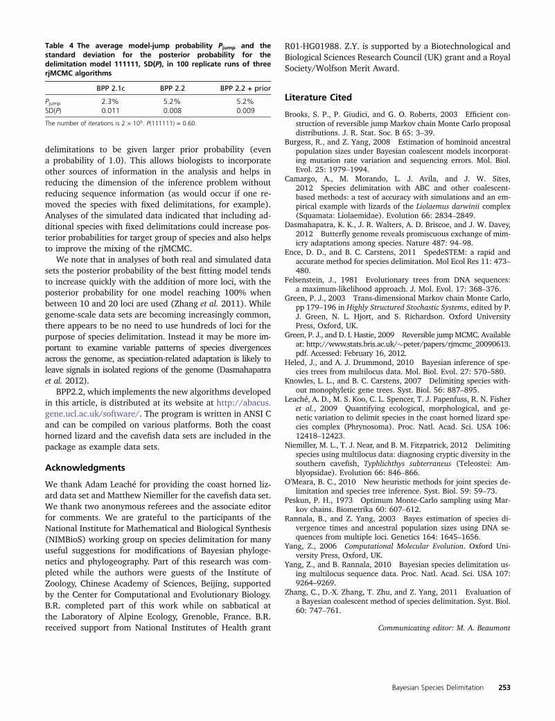
are comparable but the t’s are larger, indicating that the fishpopulations are genetically more divergent than the lizards.Computational efficiencies of the different rjMCMC algo-rithms are summarized in Table 4. Compared with BPP2.1c,the rubber-band algorithm and proportional scaling imple-mented in BPP2.2 increased the model-jump probabilityfrom 2.3 to 5.2%. The SDs for P(111111), the posteriorprobability for the-delimitation model 111111, is smallerin BPP2.2 than in BPP2.1c. The results suggest that themodifications we have introduced here generally cause bet-ter gene trees to be proposed, with improved acceptancerates, whatever the algorithm for proposing model parame-ters in the rjMCMC move (Yang and Rannala 2010).

The informative prior (Figure 5) disallows four delimita-tion models (000000, 100000, 110000, and 110001) andassigns the prior probability 0.125 to the eight remainingdelimitation models. This does not lead to improvements inthe acceptance rate or the precision of the posterior modelprobability. However, the prior constraint is effective in pre-venting the chain from getting stuck at the one-speciesmodel.

Discussion

The rjMCMC algorithm is very flexible in terms of possibleproposals. However, it often suffers from poor mixing whenapplied to real data. This is particularly true when the dataare highly informative and the posteriors of the parameterswithin each model are highly concentrated. Proposedbetween-model jumps tend to be rejected, so that the chainbecomes trapped in one model, even if that model has lowposterior probability. It is more difficult to construct efficientproposals for rjMCMC than for conventional MCMC. Inconventional MCMC, the distance between the current valueand the proposed value of a parameter can be used to adjustthe acceptance rate and to construct an optimal algorithm,but in rjMCMC we lack such a measure of distance. Forexample, in conventional MCMC using a sliding-windowproposal for a continuous target distribution, a small win-dow size will lead to small moves with Pjump � 1, whereasa large window size will lead to large moves and a smallPjump. Therefore, if the window size is adjusted to obtaina near-optimal Pjump, the conventional MCMC algorithmcan work well regardless of whether the posterior is concen-trated or diffuse. In rjMCMC, there is no obvious parallel tosuch a scale adjustment because there is no guide as to what

Table 3 The average model-jump probability Pjump and the standarddeviation for the posterior probability for the delimitation model1111, SD(P), in 100 replicate runs of three rjMCMC algorithms

N BPP 2.1c BPP 2.2 BPP 2.2 + prior

Pjump 1.4% 7.6% 7.6%SD(P) 2 · 105 0.024 0.014 0.015SD(P) 8 · 105 0.010 0.007 0.007

P(1111) = 0.58. N is the chain length (the number of iterations).

Bayesian Species Delimitation 251

is a “local move” when the chain is jumping between mod-els. As Green and Hastie (2009) pointed out, “For across-model proposals the lack of a concept of closeness meansthat frequently it is the problem of low acceptance probabil-ities that makes efficient proposals hard to design; it is usualfor across-model moves to display much lower acceptanceprobabilities than within-model moves.”

We note here several important differences betweenconventional MCMC and cross-model rjMCMC. First, forwithin-model MCMC, there is an optimal acceptance pro-portion (say �30–40% for 1-D moves). For cross-modelrjMCMC, the higher Pjump is, the more efficient the chaintends to be (Peskun 1973). Second, Pjump is maximized byproposing parameters for the new model from its posterior.Third, for conventional MCMC, Pjump can be made arbitrarilyclose to 1 by decreasing the step size. With rjMCMC, theposterior model probabilities place an upper bound on Pjump;it cannot exceed twice one minus the posterior probability ofthe best-fitting model. Thus Pjump � 0 does not necessarilymean poor mixing. If the best model has posterior probabil-ity 99.9%, the chain must stay in the model 99.9% of thetime and it therefore cannot accept .�0.1% of the pro-posals to move away from it.

With conventional MCMC, taking a sufficiently small stepvirtually guarantees acceptance (although the resultingchain may mix slowly). One might think that the samewould apply to rjMCMC and that to move from a simpler

model (with fewer parameters) to a more complex one(with more parameters), proposing parameter values for themore complex model that closely correspond to the currentparameters of the simpler model would guarantee accep-tance. This is not the case for rjMCMC, yet it appears to bea widespread misconception concerning rjMCMC proposals.For example, Brooks et al. (2003) describe a “weak non-identifiability centering” proposal based on this idea thatthey claim will lead to high probabilities of between-modeljumps (in fact, they argue that between-model acceptancerates of 1 can be achieved using this proposal). Clearly this isincorrect because the acceptance rate is always limited bythe posterior probability of the best model. If one modeldominates in the posterior, the acceptance rate of be-tween-model moves can never be high. The prior, if it isdiffuse, also works against the parameter-rich model. Eventhough the likelihood stays essentially the same, the pro-posal is very likely to be rejected.

The mixing problems discussed here are due to thechange of dimensions and/or change of probability spacesin between-model moves, that is, the change from theprobability space of one model to the probability space ofanother model. Here we are not using Green’s formalism inwhich all models share one general space (Green and Hastie2009), but consider each model having its own probabilityspace. Mixing problems can arise in moves between modelsof the same dimension, but a change of dimension introdu-ces additional difficulty. While Green (2003) suggested thatmixing problems may have more to do with high dimension-ality than with change of dimension, our experience issomewhat different. The within-model MCMC algo-rithms implemented in BPP have been successfully used toanalyze as many as 50,000 loci (Burgess and Yang 2008),which involves extremely high dimensions in the gene treesand node ages, but the program may begin to have mixingproblems with small numbers of loci when using rjMCMCfor species delimitation.

Recognizing the difficulty of achieving generic improve-ments to rjMCMC algorithms due to some of the problemsoutlined above, in this article we focused on improving therjMCMC mixing of the species-delimitation program bymaking algorithmic modifications that are specific to ourparticular model. First, we have modified our algorithm tojointly propose divergence times and multilocus gene treesto reduce the strong constraint that species divergence timevs. gene-tree conflicts impose during the split move, whichleads to reduced acceptance rates. This constraint becomesincreasingly severe with the addition of more loci and/orsequences in the old algorithm. The rubber-band algorithmwe implemented helps to reduce the effect of this constraintand results in a several-fold improvement in the accep-tance rates of between-model jumps. The between-modeljump acceptance rates are still often much less than thetheoretical maximum, however, suggesting that otherimprovements remain to be found. A second modificationchanged the prior on the guide tree to allow certain species

Figure 5 The guide tree for seven populations of cavefish (Typhlichthys),from Niemiller et al. (2012). Estimates of u’s for modern (in parentheses)as well as ancestral populations under the multi-species coalescent modelare shown, as well as estimates of t’s, all measured by the expectednumber of mutations per kilobase. In the species-delimitation analysis(using the new prior), probabilities were assigned to the nodes as ((((A,E):0.5, (B, F):0.5):1.0, (C, D):0.5):1.0, Sp):1.0, so that four species-delim-itation models 000000, 100000, 110000, and 110001 are disallowed bythe prior while the other eight are assigned prior probability 0.125 each.

252 B. Rannala and Z. Yang

delimitations to be given larger prior probability (evena probability of 1.0). This allows biologists to incorporateother sources of information in the analysis and helps inreducing the dimension of the inference problem withoutreducing sequence information (as would occur if one re-moved the species with fixed delimitations, for example).Analyses of the simulated data indicated that including ad-ditional species with fixed delimitations could increase pos-terior probabilities for target group of species and also helpsto improve the mixing of the rjMCMC.

We note that in analyses of both real and simulated datasets the posterior probability of the best fitting model tendsto increase quickly with the addition of more loci, with theposterior probability for one model reaching 100% whenbetween 10 and 20 loci are used (Zhang et al. 2011). Whilegenome-scale data sets are becoming increasingly common,there appears to be no need to use hundreds of loci for thepurpose of species delimitation. Instead it may be more im-portant to examine variable patterns of species divergencesacross the genome, as speciation-related adaptation is likely toleave signals in isolated regions of the genome (Dasmahapatraet al. 2012).

BPP2.2, which implements the new algorithms developedin this article, is distributed at its website at http://abacus.gene.ucl.ac.uk/software/. The program is written in ANSI Cand can be compiled on various platforms. Both the coasthorned lizard and the cavefish data sets are included in thepackage as example data sets.

Acknowledgments

We thank Adam Leaché for providing the coast horned liz-ard data set and Matthew Niemiller for the cavefish data set.We thank two anonymous referees and the associate editorfor comments. We are grateful to the participants of theNational Institute for Mathematical and Biological Synthesis(NIMBioS) working group on species delimitation for manyuseful suggestions for modifications of Bayesian phyloge-netics and phylogeography. Part of this research was com-pleted while the authors were guests of the Institute ofZoology, Chinese Academy of Sciences, Beijing, supportedby the Center for Computational and Evolutionary Biology.B.R. completed part of this work while on sabbatical atthe Laboratory of Alpine Ecology, Grenoble, France. B.R.received support from National Institutes of Health grant

R01-HG01988. Z.Y. is supported by a Biotechnological andBiological Sciences Research Council (UK) grant and a RoyalSociety/Wolfson Merit Award.

Literature Cited

Brooks, S. P., P. Giudici, and G. O. Roberts, 2003 Efficient con-struction of reversible jump Markov chain Monte Carlo proposaldistributions. J. R. Stat. Soc. B 65: 3–39.

Burgess, R., and Z. Yang, 2008 Estimation of hominoid ancestralpopulation sizes under Bayesian coalescent models incorporat-ing mutation rate variation and sequencing errors. Mol. Biol.Evol. 25: 1979–1994.

Camargo, A., M. Morando, L. J. Avila, and J. W. Sites,2012 Species delimitation with ABC and other coalescent-based methods: a test of accuracy with simulations and an em-pirical example with lizards of the Liolaemus darwinii complex(Squamata: Liolaemidae). Evolution 66: 2834–2849.

Dasmahapatra, K. K., J. R. Walters, A. D. Briscoe, and J. W. Davey,2012 Butterfly genome reveals promiscuous exchange of mim-icry adaptations among species. Nature 487: 94–98.

Ence, D. D., and B. C. Carstens, 2011 SpedeSTEM: a rapid andaccurate method for species delimitation. Mol Ecol Res 11: 473–480.

Felsenstein, J., 1981 Evolutionary trees from DNA sequences:a maximum-likelihood approach. J. Mol. Evol. 17: 368–376.

Green, P. J., 2003 Trans-dimensional Markov chain Monte Carlo,pp 179–196 in Highly Structured Stochastic Systems, edited by P.J. Green, N. L. Hjort, and S. Richardson. Oxford UniversityPress, Oxford, UK.

Green, P. J., and D. I. Hastie, 2009 Reversible jumpMCMC. Availableat: http://www.stats.bris.ac.uk/�peter/papers/rjmcmc_20090613.pdf. Accessed: February 16, 2012.

Heled, J., and A. J. Drummond, 2010 Bayesian inference of spe-cies trees from multilocus data. Mol. Biol. Evol. 27: 570–580.

Knowles, L. L., and B. C. Carstens, 2007 Delimiting species with-out monophyletic gene trees. Syst. Biol. 56: 887–895.

Leaché, A. D., M. S. Koo, C. L. Spencer, T. J. Papenfuss, R. N. Fisheret al., 2009 Quantifying ecological, morphological, and ge-netic variation to delimit species in the coast horned lizard spe-cies complex (Phrynosoma). Proc. Natl. Acad. Sci. USA 106:12418–12423.

Niemiller, M. L., T. J. Near, and B. M. Fitzpatrick, 2012 Delimitingspecies using multilocus data: diagnosing cryptic diversity in thesouthern cavefish, Typhlichthys subterraneus (Teleostei: Am-blyopsidae). Evolution 66: 846–866.

O’Meara, B. C., 2010 New heuristic methods for joint species de-limitation and species tree inference. Syst. Biol. 59: 59–73.

Peskun, P. H., 1973 Optimum Monte-Carlo sampling using Mar-kov chains. Biometrika 60: 607–612.

Rannala, B., and Z. Yang, 2003 Bayes estimation of species di-vergence times and ancestral population sizes using DNA se-quences from multiple loci. Genetics 164: 1645–1656.

Yang, Z., 2006 Computational Molecular Evolution. Oxford Uni-versity Press, Oxford, UK.

Yang, Z., and B. Rannala, 2010 Bayesian species delimitation us-ing multilocus sequence data. Proc. Natl. Acad. Sci. USA 107:9264–9269.

Zhang, C., D.-X. Zhang, T. Zhu, and Z. Yang, 2011 Evaluation ofa Bayesian coalescent method of species delimitation. Syst. Biol.60: 747–761.

Communicating editor: M. A. Beaumont

Table 4 The average model-jump probability Pjump and thestandard deviation for the posterior probability for thedelimitation model 111111, SD(P), in 100 replicate runs of threerjMCMC algorithms

BPP 2.1c BPP 2.2 BPP 2.2 + prior

Pjump 2.3% 5.2% 5.2%SD(P) 0.011 0.008 0.009

The number of iterations is 2 · 105. P(111111) = 0.60.

Bayesian Species Delimitation 253