option pricing in some non-lévy jump models

OPTION PRICING IN SOME NON-LEVY JUMP MODELS

LINGFEI LI∗ AND GONGQIU ZHANG†

Abstract. This paper considers pricing European options in a large class of one-dimensionalMarkovian jump processes known as subordinate diffusions, which are obtained by time changing adiffusion process with an independent Levy or additive random clock. These jump processes are non-Levy in general, and they can be viewed as natural generalization of many popular Levy processesused in finance. Subordinate diffusions offer richer jump behavior than Levy processes and theyhave found a variety of applications in financial modelling. The pricing problem for these processespresents unique challenges as existing numerical PIDE schemes fail to be efficient and the applicabilityof transform methods to many subordinate diffusions is unclear. We develop a novel method basedon finite difference approximation of spatial derivatives and matrix eigendecomposition, and it candeal with diffusions that exhibit various types of boundary behavior. Since financial payoffs aretypically not smooth, we apply a smoothing technique and use extrapolation to speed up convergence.We provide convergence and error analysis and perform various numerical experiments to showthe proposed method is fast and accurate. Extension to pricing path-dependent options will beinvestigated in a follow-up paper.

Key words. jump processes, option pricing, time change, finite difference, matrix eigendecom-position.

AMS subject classifications. 60J60, 60J75, 91G20, 91G60.

1. Introduction. Jump processes are an essential modelling tool in finance andpopular financial models with jumps are often based on Levy processes. There is anextensive literature on the study of Levy processes and their applications in finance(see the monograph [6] and [13]). To price options in Levy-driven models, numericalmethods based on transforms (e.g., [11], [43], [20, 21], [22, 24], [7]) and numericalschemes for partial integro-differential equations (PIDEs) (e.g., [1], [16], [14], [23]) aredeveloped. However, jumps of Levy processes are independent of the state, which canbe quite unrealistic in some applications.

This paper develops a fast and accurate numerical method for pricing options inmodels based on one-dimensional (1D) subordinate diffusions. The problem presentsunique challenges as existing numerical PIDE schemes fail to be efficient and the ap-plicability of transform methods to many subordinate diffusions is unclear. A 1D sub-ordinate diffusion is obtained by time changing a 1D diffusion process (it will be calledbackground diffusion hereafter) with an independent Levy or additive random clock(i.e., a nonnegative Levy/additive process; also called Levy/additive subordinator inthe literature). We shall add “Levy” or “additive” before “subordinate diffusion” toindicate which type of subordinator is used if needed. Subordinate diffusions form alarge class of Markovian jump processes whose jumps are generally state-dependent,hence they offer richer jump behavior than Levy processes. Their jumps can exhibit avariety of interesting behavior. For example, jumps can have finite or infinite activity,and have finite or infinite variation (recent high-frequency statistical analysis favorsinfinite activity pure jump processes with infinite variation in some applications; see[56]). Jumps of subordinate diffusion are mean-reverting if the background diffusionis so, and this fact has been exploited by [36] for commodity modelling. Applying

∗Department of Systems Engineering and Engineering Management, The Chinese University ofHong Kong, Shatin, Hong Kong. Email: [email protected].†Department of Systems Engineering and Engineering Management, The Chinese University of

Hong Kong, Shatin, Hong Kong. Email: [email protected].

1

2 Option Pricing in Some Non-Levy Jump Models

subordination to diffusions on a bounded interval is also a natural approach to con-struct jump processes with bounds, which are useful for modelling financial variablesthat move in bounded zones (e.g., asset prices in a highly competitive market andexchange rates in a target zone). A series of papers have already established the use-fulness of subordinate diffusions in financial applications, and in our opinion they canbe viewed as nice additions to Levy processes for modelling jumps. See [3], [46], [36],[5], [41] and [48] for applications of Levy subordinate diffusions in a variety of marketsand [38], [32], [33] for applications of additive subordinate diffusions. Many popularLevy processes in finance can be represented as a Brownian motion time changedby an independent Levy subordinator, including VG, NIG, CGMY, hyperbolic andMeixner processes ([44]). Therefore subordinate diffusions can be viewed as a naturalgeneralization of many Levy processes by time changing more general diffusions.

Existing applications of subordinate diffusions in finance focus on analyticallytractable specifications whose transition operator admits an eigenfunction expansionwith known eigenvalues and eigenfunctions. European options can be priced analyti-cally using eigenfunction expansions in these models. This approach has been furtherextended in several works ([34, 35, 37, 40]) to price Bermudan, American, barrier,swing and real options in these models.

Restricting to analytically tractable specifications of subordinate diffusions formodelling limits the choice of the background diffusion, and such models may fail tocapture important features. The analytical approach using eigenfunction expansionsis not applicable to general subordinate diffusions, which motivates us to develop afast and accurate numerical method that is generally applicable.

The rest of the paper is organized as follows. In Section 2, we introduce subordi-nate diffusions and explain why existing numerical methods are not applicable or donot solve our problem efficiently. Section 3 presents our numerical method for pric-ing European options and provide convergence and error analysis. Section 4 presentsvarious numerical examples which confirm the computational efficiency and accuracyof our method, and comparison to a popular existing PIDE scheme is given. Section5 concludes the paper and the appendix contains the proof for lemmas.

2. Subordinate Diffusions. Let X be a one-dimensional time-homogeneousdiffusion living in an interval I with end-points l and r (−∞ ≤ l < r ≤ ∞), andfor f ∈ C2

c ((l, r)) (twice-continuously differentiable functions on (l, r) with compactsupport), its infinitesimal generator G takes the form

Gf(x) =1

2σ2(x)f ′′(x) + µ(x)f ′(x)− k(x)f(x) for f ∈ C2

c ((l, r)),

where µ(x), σ2(x), k(x) are known as the drift, diffusion coefficient and killing rate,respectively. We assume that for x ∈ (l, r), µ(x), σ(x) and k(x) are continuous, andσ(x) > 0, k(x) ≥ 0. We also assume that X is regular, i.e., for any x, y ∈ (l, r), Xcan reach y starting from x in finite time with positive probability.

Whether an end-point is included in I depends on the boundary behavior. If it isinfinite, we assume it is inaccessible, i.e., starting from any point in (l, r), X cannotreach the boundary in finite time with positive probability. If it is finite, the boundarybehavior can be either natural, exit, entrance, regular specified as killing or reflecting.We refer readers to e.g., [4, Chapter II.6] for Feller’s classification of boundaries andconditions to determine the boundary behavior. Upon hitting the exit and killingboundary, X is sent immediately to the cemetery state ∆. Alternatively X can bekilled by the additive functional

∫ t0k(Xu)du, where k is the killing rate, i.e., X is sent

L. Li and G. Zhang 3

to ∆ at time τk := inf{t ≥ 0 :

∫ t0k(Xu)du ≥ e

}, where e is an exponential random

variable with unit mean and independent of X. The lifetime of X, denoted by ζ, isequal to the first time X is killed at the boundary or τk, whichever is smaller. Notethat killing is a natural way to model bankruptcy risk (see e.g., [10]). This frameworkencompasses many diffusions used in finance.

A Levy subordinator is a stochastically continuous process with independent andstationary increments that starts at zero and is non-negative (see [13, Definition 3.1]).Non-negativity implies that it is non-decreasing ([13, Proposition 3.10]). Consider aLevy subordinator T and let qt(·) be the probability distribution of Tt, which isunknown in general. However the Laplace transform of T is known and given by theLevy-Khintchine formula ([13, Proposition 3.10])

E[e−λTt ] =

∫[0,∞)

e−λsqt(ds) = e−φ(λ)t, φ(λ) = γλ+

∫(0,∞)

(1− e−λs)ν(ds),

Here γ ≥ 0 is the drift of the subordinator and ν is the Levy measure satisfying∫(0,∞)

(s∧1)ν(ds) <∞. For typical Levy subordinators used in finance, the integral in

φ(λ) can be further reduced to a closed-form expression. Popular choices are temperedstable Levy subordinators, whose Levy measures are given by ν(ds) = Cs−p−1e−ηs

with C > 0, 0 < p < 1, η > 0. For them, φ(λ) = γλ − CΓ(−p)[(λ + η)p − λp] whereΓ(·) is the gamma function.

We assume X and T are independent and define Xφt := XTt . This time change

technique is called Bochner’s subordination and has been extensively studied in themathematics literature (see [54]). Xφ is called Levy subordinate diffusion, and thesuperscript φ indicates the Laplace exponent of T . It is a time-homogenous Markovprocess with lifetime given by ζφ = inf{t ≥ 0 : Tt ≥ ζ}. The infinitesimal generatorof Xφ is given in [34, p.631], which is an integro-differential operator. In particularits jump density is state-dependent in general and is given by

πφ(x, y) =

∫(0,∞)

p(s, x, y)ν(ds), (2.1)

where p(s, x, y) is the transition probability density of X.[32] proposes to construct time dependent jump processes by time changing a

diffusion X with an independent additive subordinator T (an additive subordinatoris basically a Levy subordinator without stationary increments). The resulting pro-cesses, called additive subordinate diffusions, generalize Levy subordinate diffusionsby having time dependence and they provide good fit to the implied volatility surfacewhile Levy subordinate diffusions typically only fit volatility smiles/skews of a singlematurity well. We refer readers to [32] for detailed discussion. Like Levy subordina-tors, the Laplace transform of additive subordinators is known analytically. In therest of the paper, we focus on Levy subordinate diffusions. Our method extends di-rectly to additive subordinate diffusions and the only change is to replace the Laplacetransform of the Levy subordinator by that of the additive subordinator.

To obtain the price of an European option with payoff function f , we need tocompute e−rtEx[f(Xφ

t )] under the risk-neutral measure (the risk-free interest rate ris assumed to be constant). This expectation can be decomposed into two parts:

Ex[f(Xφt )] = Ex[f(Xφ

t )1{ζφ>t}] + f(∆)Ex[1{ζφ≤t}]

= Ex[f(Xφt )1{ζφ>t}] + f(∆)− f(∆)Ex[1{ζφ>t}].


Therefore to price European options, we only need to compute

uφ(t, x) := Ex[f(Xφt )1{ζφ>t}]. (2.2)

To illustrate the inefficiency of existing numerical PIDE schemes in obtaining theEuropean option price uφ(t, x), let’s for the moment, assume that uφ(t, x) is a classicalsolution to a PIDE (in general the European option price is not a classical solution toa PIDE; sufficient conditions for it to hold can be found in e.g., [15, Proposition 2] forLevy processes and [52, Theorem 7] for general SDEs with jumps). There already existmany numerical schemes for solving PIDEs. See, for example, [1], [14], [16] and [23].To apply these schemes requires the value of the jump density πφ(x, y) for differentx and y on a grid. In our case, πφ(x, y) =

∫(0,∞)

p(τ, x, y)ν(dτ) (see (2.1)), which

cannot be obtained in closed form in general. One can certainly compute πφ(x, y)by numerical integration, which requires the value of the diffusion transition densityp(τ, x, y) for different τ in a large region to obtain high accuracy (here ν(·) is known).But p(τ, x, y) is in general unknown, and has to be computed by numerically solvingthe PDE it satisfies. If the forward PDE is used, for fixed x, we need to solve thePDE numerically over a long time horizon, and this has to be repeated for differentx on the grid. Apparently, this procedure is inefficient as it requires very intensivecomputations. The above discussion was based on the assumption that uφ(t, x) is aclassical solution to a PIDE. More generally, uφ(t, x) may not even be differentiable inx for typical payoffs in finance, let alone being a classical solution. An example is givenby the pure jump VG process, which is obtained by time changing a BM with a driftlessGamma subordinator ([15, p.307]). In general, uφ(t, x) can only be interpreted as aviscosity solution to the PIDE. See [15, Proposition 8] for results in exponential Levymodels and a convergent scheme is developed in [14] to find the viscosity solution inthese models. For some existing PIDE schemes, since it is not clear whether they areconvergent for finding the viscosity solution, their applicability to pricing Europeanoptions for general subordinate diffusions is even called into question. As for transformmethods, they can be applied to subordinate diffusions with an explicit expression forthe characteristic function. This is true in e.g., many subordinate Brownian motionmodels. However, for many other subordinate diffusions, it is not clear how to computethe characteristic function, so the applicability of transform methods remains to bea question (see Remark 1). In this paper, we will develop an efficient method whichdoes not require the smoothness of uφ(t, x) (in particular our method applies to theVG model) and the value of the jump density πφ(x, y).

Remark 1 (characteristic function for subordinate diffusions). When X is a

Brownian motion with drift µ and volatility σ, the characteristic function E[eiuXφt ] =

E[E[eiuXTt |Tt]] = E[eiuµTt−(1/2)u2σ2Tt ] = e−φ(1/2u2σ2−iuµ), which has a closed-formexpression if φ does. When X is an affine diffusion, its characteristic function can becomputed by solving the associated Riccati equations and if qt, the distribution of Tt is

known, one can use numerical quadrature to compute E[eiuXφt ] =

∫[0,∞)

E[eiuXs ]qt(ds)

(this idea has been used in [39] where the Gamma subordinator is used; in this case qtis a Gamma distribution and Gauss-Laguerre quadrature can be applied to efficientlycompute the integral). For these cases, one can apply various transform methods tocompute option prices efficiently and the method developed in this paper can be viewedas an alternative. However, there are also many financial applications where thediffusion is non-affine (see e.g., [12], [46]) and the distribution of the subordinatoris unknown (this is the case for tempered stable subordinators with p 6= 1/2). So for


these cases, it is unclear how the characteristic function of Xφt can be computed and

hence the applicability of transform methods is unclear.

3. European Option Pricing in Subordinate Diffusion Models. We wantto compute uφ(t, x) defined in (2.2) for a general Levy subordinate diffusion Xφ.Define u(s, x) = Ex[f(Xs)1{ζ>s}], where ζ is the lifetime of the background diffusion

X. Since Xφ = XTt with X,T independent, we have

uφ(t, x) =

∫[0,∞)

u(s, x)qt(ds).

For the class of diffusions we consider (see Section 2), u(s, x) is the solution to thefollowing PDE for a large class of payoff functions (for instance when f is continuousand bounded on (l, r); see [45]):

∂tu(t, x) = µ(x)∂xu(t, x) +1

2σ2(x)∂xxu(t, x)− k(x)u(t, x), t > 0, x ∈ (l, r), (3.1)

u(0, x) = f(x), x ∈ (l, r).

We will specify boundary conditions for the PDE to correctly capture the boundarybehavior in Section 3.2. The key idea of our numerical method is to develop anapproximation for the value function of the diffusion PDE that is easy to generalizeafter subordination. To do that, we first localize the problem when infinite boundarypoints are present. We then consider the diffusion PDE problem on a finite interval.We approximate the spatial derivatives by finite difference which leads us to an ODEsystem in time, for which we find the solution using matrix eigendecomposition. Foran n × n matrix, eigendecomposition typically requires O(n3) works. We show howto do it in O(n2) in our case. Since time enters the approximate solution for thediffusion PDE in an exponential form, using the analytical knowledge of the Laplacetransform of the subordinator, we immediately obtain an approximation for the valuefunction of the subordinate diffusion. The proposed method will be termed as thefinite difference-eigendecomposition (FDEIG) algorithm.

3.1. Localization of infinite boundaries. We start by considering the casel = −∞ and r = ∞ (the case where only one of them is infinite can be dealt withsimilarly). By our assumption, they are inaccessible. We consider a new diffusion XA

with lower boundary −A and upper boundary A, where A is sufficiently large. XA

has the same drift, diffusion coefficient and killing rate as X in (−A,A), and −A andA are regular boundaries which can be either specified as killing or reflecting. LetζA, ζφ,A be the lifetime of process XA

t and Xφ,At := XA

Tt, respectively. Define

uA(t, x) := Ex[f(XAt )1{ζA>t}], u

φA(t, x) := Ex[f(Xφ,A

t )1{ζφ,A>t}].

We introduce the pre-default process of X, denoted by X, which has the same driftand diffusion coefficient as X but zero killing rate, hence its lifetime is infinite. Weassume that −∞,∞ are inaccessible boundaries of X. Similarly, XA is the pre-defaultprocess of XA. However, unlike X, XA can have finite lifetime because it is killed onthe boundary if A and −A are specified as killing. Let Ms,x = sup0≤u≤s |Xu|. Wefirst provide an estimate for |uA(s, x) − u(s, x)| in Lemma 3.1, based on which we

show the convergence of uφA(t, x).Lemma 3.1. Assume that f is nonnegative and monotone on R. Then for any

(s, x) ∈ (0,∞)× (−A,A),

|uA(s, x)− u(s, x)| ≤ Ex[(f(Xs) + f(Ms,x) + f(−Ms,x))1{Ms,x≥A}].


When A and −A are killing boundaries, f(Ms,x)+f(−Ms,x) on the RHS is not needed.Alternatively, assume that f is bounded on R and we denote its L∞-norm by ‖f‖∞.Then for any (s, x) ∈ (0,∞)× (−A,A),

|uA(s, x)− u(s, x)| ≤ 2 ‖f‖∞ Px (Ms,x ≥ A) . (3.2)

Proposition 3.2. Assume either f is nonnegative and monotone on R and forany (s, x) ∈ [0,∞) × R, Ex[f(Xs)], Ex[f(−Ms,x)], Ex[f(Ms,x)] are finite or assume

that f is bounded on R. Then for any (t, x) ∈ [0,∞) × R, uφA(t, x) → uφ(t, x) whenA→∞.

Proof. We first prove the claim under the second assumption. Since −∞,∞are inaccessible for X, Px(Ms,x ≥ A) → 0 as A → ∞. From (3.2), this impliesuA(s, x)→ u(s, x). From the time-change construction, we have

|uφA(t, x)− uφ(t, x)| ≤∫

[0,∞)

|uA(s, x)− u(s, x)|qt(ds). (3.3)

Since f is bounded, u and uA are bounded. Hence by dominated convergence theorem,uφA(t, x)→ uφ(t, x). Under the first assumption, by dominated convergence theorem,

Ex[f(Xs)1{Ms,x≥A}]→ 0, Ex[f(Ms,x)1{Ms,x≥A}]→ 0, Ex[f(−Ms,x)1{Ms,x≥A}]→ 0

when A→∞. Then from Lemma 3.1 and monotone convergence theorem,

|uφA(t, x)− uφ(t, x)| ≤∫

[0,∞)

Ex[f(Xs)1{Ms,x≥A}]qt(ds)

+

∫[0,∞)

Ex[f(Ms,x)1{Ms,x≥A}]qt(ds) +

∫[0,∞)

Ex[f(−Ms,x)1{Ms,x≥A}]qt(ds)

which goes to 0 when A→∞.We call |uφA(t, x) − uφ(t, x)| as the localization error. Under further conditions

on µ and σ, we show that the localization error decays exponentially based on anestimate of Px(Ms,x ≥ A).

Proposition 3.3. Suppose X is the unique weak solution in law to the SDEdXt = µ(Xt)dt + σ(Xt)dWt with X0 = x. Assume that f is bounded on R and thatthere exists β > 0 such that

∫(1,∞)

eβsν(ds) <∞. Further assume that µ(x) and σ(x)

are bounded on R. Then for any x ∈ (−A,A), there exist α,C > 0 independent ofx,A such that

|uφA(t, x)− uφ(t, x)| ≤ Ce−α(A−|x|). (3.4)

Proof. Let µ := ‖µ‖∞, σ := ‖σ‖∞. From (3.2) and (3.3), we have

|uφA(t, x)− uφ(t, x)| ≤ 2 ‖f‖∞∫

[0,∞)

Px [Ms,x ≥ A] qt(ds)

≤ 2 ‖f‖∞ e−αA∫

[0,∞)

Ex [exp(αMs,x)] qt(ds). (3.5)


for α > 0. In the second step, we used the Chebyshev inequality. The choice of α willbe specified later. Below we estimate Ex [exp(αMs,x)]. Notice that for any s ≥ 0,

sup0≤u≤s

|Xu| = sup0≤s≤u

∣∣∣∣x+

∫ s

0

µ(Xu)du+

∫ s

0

σ(Xu)dWu

∣∣∣∣≤ |x|+ sup

0≤u≤s

∣∣∣∣∫ s

0

σ(Xu)dWu

∣∣∣∣+ µs,

which implies Px(Ms,x ≥ z) ≤ Px(

sup0≤u≤s

∣∣∣∫ s0 σ(Xu)dWu

∣∣∣ ≥ z − µs− |x|). Hence,

Ex[exp(αMs,x)] =

∫ ∞0

Px(exp(αMs,x) ≥ z) dz

≤∫ ∞

0

Px

(sup

0≤u≤s

∣∣∣∣∫ s

0

σ(Xu)dWu

∣∣∣∣ ≥ ln z/α− µs− |x|)dz

≤∫ ∞

0

min

(1, 2 exp

(− (ln z/α− µs− |x|)2

2σ2s

))dz.

In the last step, we used Corollary 9.29 in [50]. Now let z∗ = exp(α(|x| + µs +√2σ2s ln 2)).

Ex[exp(αMs,x)] ≤ z∗ +

∫ ∞z∗

2 exp

(− (ln z/α− µs− |x|)2

2σ2s

)dz.

Let y = ln z/α− µs− |x| and y∗ = 2σ√s ln 2. Then,

Ex[exp(αMs,x)] ≤ exp(α(|x|+ µs+√

2σ2s ln 2)) +

∫ ∞y∗

2α exp

(− y2

2σ2s

)exp (α(µs+ |x|+ y)) dy

≤ exp(α(|x|+ µs+√

2σ2s ln 2)) + 2α exp (α(µs+ |x|))∫ ∞−∞

exp

(− y2

2σ2s+ αy

)dy

= exp(α(|x|+ µs+√

2σ2s ln 2)) + 2α exp(α(µs+ |x|) + σ2α2s/2

) ∫ ∞−∞

exp

(− (y − ασ2s)2

2σ2s

)dy

= exp(α(|x|+ µs+√

2σ2s ln 2)) + 2α exp(α(µs+ |x|) + σ2α2s/2

)√2πσ2s.

Now we choose an α > 0 such that µα + σ2α2/2 < β. It is easy to see that thereexists a constant C0 > 0 such that

exp(α(|x|+ µs+√

2σ2s ln 2))+2α exp(α(µs+ |x|) + σ2α2s/2

)√2πσ2s ≤ C0e

α|x|+βs.

By [53, Theorem 25.3], the condition∫

(1,∞)eβsν(ds) < ∞ is equivalent to E[eβTt ] =∫

[0,∞)eβsqt(ds) < ∞ for all t ≥ 0. Hence

∫[0,∞)

qt(ds)Ex[exp(αMs,x)] ≤ C1eα|x| for

some C1 > 0. Substituting this into (3.5), we arrive at (3.4) for some C > 0.Remark 2. The existence of

∫(1,∞)

eβsν(ds) < ∞ for some β > 0 is satisfied

if ν(ds) has an exponentially decaying tail, which is true in e.g., tempered stablesubordinators.

Remark 3. Let X be a diffusion with linear mean-reverting drift with boundedσ(x), i.e., dXt = κ(θ− Xt)dt+ σ(Xt)dWt (κ > 0). An important example in financeis given by the Ornstein-Uhlenbeck process for which σ(x) is a constant. For these


processes, µ(x) is not bounded. Hence Proposition 3.3 cannot be directly applied.However, in this case

Xt = x0e−κt + θ(1− e−κt) +

∫ t

0

σ(Xs)e−κ(t−s)dWs.

Therefore we can proceed in a way similar to the proof of Proposition 3.3 and showthat for such process, the localization error still decays exponentially as in (3.4).

In Section 4, we will see that even if the diffusion under consideration does notsatisfy the bounded coefficient condition in Proposition 3.3, the localization error canstill converge exponentially.

3.2. Boundary conditions for the diffusion PDE at finite boundaries.From now on, we consider a diffusion X living on a finite interval with end-point land r (if infinite boundaries are present in the problem, we localize them and considerthe localized diffusion XA). In general, the boundary behavior can be either natural,entrance, exit, killing or reflecting. We impose the following assumption from Section3.2 to 3.5. In Section 3.6, we will discuss how to extend our method when Assumption1 is violated.

Assumption 1. σ(x) ∈ C4([l, r]), µ(x) ∈ C3([l, r]), k(x) ∈ C2([l, r]), σ(x) > 0for all x ∈ [l, r].

Here Cn([l, r]) is the space of functions that are n times continuously differentiableon (l, r) and the function and its derivatives up to the n-th order have continuousextensions to l and r. The smoothness assumptions on the diffusion characteristicsare naturally satisfied in many financial models. From the conditions that determinethe boundary behavior in [4, Chapter II.6], it is easy to see that l and r can only bekilling or reflecting boundaries under Assumption 1.

We discuss what boundary conditions should be imposed for the diffusion PDE(3.1) so that the boundary behavior is correctly captured. In fact under Assump-tion 1, the PDE (3.1) holds on (l, r) for any f ∈ L2(I,m) := {f is measurable :∫If2(x)m(dx) <∞}, where m is the speed measure of X ([42, Eq.(3.3)]) and I is the

state-space (we prove it in Proposition 3.5). Below we only specify results for the leftboundary l. Results for r are entirely similar.

When l is an killing boundary, it is easy to see that

u(t, l) = 0 for all t ≥ 0,

because if the process is already at l, it is sent to the cemetery state and 1{ζ>t} = 0.We next derive the boundary condition for the reflecting case which is less obvious.

For the class of diffusion process we introduce in Section 2 (not necessarily satisfy-ing Assumption 1), its infinitesimal generator G can be extended uniquely to L2(I,m).If there are no natural boundaries, the spectrum of G is purely discrete and simple([42, Theorem 3.2]), and for payoff function f ∈ L2(I,m),

u(t, x) =

∞∑n=1

fneλntϕn(x), fn =

∫I

f(x)ϕn(x)m(dx). (3.6)

Here λn and ϕn are the n-th eigenvalue and eigenfunction for G, respectively, withλn ≤ 0 and

∫Iϕ2n(x)m(dx) = 1 (i.e., ϕn is normalized). They are solutions to the

Sturm-Liouville (S-L) eigenvalue problem

1

2σ2(x)ϕ′′(x) + µ(x)ϕ′(x)− k(x)ϕ(x) = λϕ(x)


with appropriate boundary conditions at l and r (see e.g., [42] Section 3.3):• l is killing: ϕ(l) = 0.

• l is reflecting: limx→lϕ′(x)s(x) = 0, where s(x) is the scale density of X.

In general, the eigenvalues and eigenfunctions cannot be found out explicitly, butone can obtain estimates for them. To derive the boundary condition for u(t, x) atreflecting boundaries, we make use of (3.6) and these estimates. Under Assumption1, the S-L problem becomes a regular one that can be converted into Liouville normalform ([25, Eq. (2.1i) to (2.9)]), and the condition limx→l ϕ

′(x)/s(x) = 0 is equivalentto ϕ′(l) = 0 (as limx→l s(x) 6= 0). The next lemma obtains estimates for λn, ϕnand its derivatives based on results from regular S-L theory, which are crucial forderiving the PDE boundary condition. We will also need them later when analyzingthe convergence rate of the discretization scheme.

Lemma 3.4. Suppose Assumption 1 hold. Consider the regular S-L problem12σ

2(x)ϕ′′(x) + µ(x)ϕ′(x)− k(x)ϕ(x) = −λϕ(x), x ∈ [l, r],

ϕ(x0) = 0, if x0 is killing, x0 ∈ {l, r},ϕ′(x0) = 0, if x0 is reflecting, x0 ∈ {l, r}.

Its eigenvalues satisfy 0 ≥ λ1 > λ2 > · · · , and λn = O(−n2). For the correspondingnormalized eigenfunctions (ϕn)n≥1, there exists a constant C > 0 such that for all

n ≥ 1, ‖ϕ(k)n ‖∞ ≤ Cnk (k = 0, 1, 2, 3, 4). Here ϕ(k) is the k-th order derivative of ϕ

for k ≥ 1 and ϕ(0) is ϕ itself.Using Lemma 3.4, we now prove the following.Proposition 3.5. Under Assumption 1, the PDE (3.1) is valid on [l, r] for any

f ∈ L2(I,m). If l is reflecting, for any t > 0, ∂xu(t, l) = 0 and the PDE at l reducesto ∂tu(t, l) = 1

2σ2(l)∂xxu(t, l)− k(l)u(t, l).

Proof. For f ∈ L2(I,m), u(t, x) is represented by (3.6) for all x ∈ [l, r]. ByCauchy-Schwartz inequality, |fn| ≤ ‖f‖2 (the L2-norm of f). From the estimates ofλn and ϕn in Lemma 3.4, the series

∞∑n=1

fneλntϕ′n(x),

∞∑n=1

fneλntϕ′′n(x),

n∑n=1

fnλneλntϕn(x)

converge absolutely and uniformly in x. Hence we can interchange summation anddifferentiation and for x ∈ [l, r],

∂xu(t, x) =

∞∑n=1

fneλntϕ′n(x), ∂xxu(t, x) =

∞∑n=1

fneλntϕ′′n(x), ∂tu(t, x) =

n∑n=1

fnλneλntϕn(x).

Using the S-L equation for ϕn shows that the PDE holds on [l, r]. If l is reflect-ing, since ϕ′n(l) = 0, we have ∂xu(t, l) = 0 and the PDE at l becomes ∂tu(t, l) =12σ

2(l)∂xxu(t, l)− k(l)u(t, l).Remark 4. When l is a reflecting boundary, the condition ∂xu(t, l) = 0 alone

suffices to characterize the boundary behavior. This condition can also be found in[28, p.330], but no proof is given there. The fact that the PDE holds at l is not givenin [28] and we do not see any proof for this fact in the literature. From the numericalperspective, it is important to know the PDE is valid at l, which will be used in ourdiscretization scheme.

To summarize, the following boundary conditions are imposed for the diffusionPDE:


• l is killing: u(t, l) = 0 for t ≥ 0.• l is reflecting: ∂tu(t, l) = 1

2σ2(l)∂xxu(t, l)−k(l)u(t, l) for t > 0, u(0, l) = f(l).

Note that when l is killing, in general u(0, l) 6= f(l) as u(0, l) = 0 while f(l) isnot necessarily zero.

3.3. Discretization by finite difference. We continue our discussions underAssumption 1. To obtain a numerical approximation for u(t, x), we discretize the spacevariable x in the diffusion PDE. To simplify the exposition, we consider a uniformgrid on [l, r], with h = (r − l)/N and xi = l + ih for i = 0, 1, · · · , N . However, non-uniform grids can also be used in our method and the extension is straightforward.We approximate the partial derivatives w.r.t. x by central differences, i.e. for 1 ≤ i ≤N − 1, t > 0,

µ(xi)∂xu(t, xi) +1

2σ2(xi)∂xxu(t, xi)− k(xi)u(xi)

≈ µ(xi)u(t, xi+1)− u(t, xi−1)

2h+

1

2σ2(xi)

u(t, xi+1)− 2u(t, xi) + u(t, xi−1)

h2− k(xi)u(t, xi).

To complete the discretization, we need to deal with boundary conditions. When lis killing boundary, we simply set u(t, x0) = 0. When l is reflecting, we approximate12σ

2(l)∂xxu(t, l)− k(l)u(t, l) as follows:

1

2σ2(x0)∂xxu(t, x0)− k(x0)u(t, x0) ≈ σ2(x0)

u(t, x1)− u(t, x0)

h2− k(x0)u(t, x0),

where to approximate ∂xxu(t, x0), we expand u(t, x1) at x = x0 and use ∂xu(t, x0) = 0.The discretization scheme yields a semi-discrete system in RN+1:

d

dtuh(t) = Guh(t), uh(0) = fh. (3.7)

Here G is an (N + 1)× (N + 1) tridiagonal matrix and it has the following entries: for1 ≤ i ≤ N − 1, Gi,i±1 = [±µ(xi)/h+ σ2(xi)/h

2]/2, Gi,i = −σ2(xi)/h2 − k(xi). If x0

is killing, then G0,i = 0 for 0 ≤ i ≤ N . If x0 is reflecting, G0,0 = −σ2(x0)/h2− k(x0),G0,1 = σ2(x0)/h2. In both cases, G0,i = 0 for 2 ≤ i ≤ N . The formulae for entries atxN are entirely similar and hence they are omitted here. fh is a (N + 1)× 1 vector,with fh,i = f(xi) for 1 ≤ i ≤ N − 1. When l, r are killing, fh,0 = fh,N = 0, and whenl, r are reflecting, fh,0 = f(l) and fh,N = f(r).

3.4. Eigendecomposition. The solution to the semi-discrete system (3.7) isgiven by uh(t) = eGtfh, where eGt is the matrix exponential defined by

eGt =

∞∑n=0

tn

n!Gn. (3.8)

In the following, we derive another representation for uh(t), using which we can com-pute

∫[0,∞)

uh(s)qt(ds) analytically using the Laplace transform of the subordinator.

Before proceeding, we observe that when x0 is a killing boundary, the value forthe entries of eGtij with 1 ≤ i, j ≤ N (the (i, j)-th entry of eGt) does not depend

on the 0-th column and the 0-th row of G. Furthermore, f0h = 0 (the 0-th entry of

fh). Therefore, to compute the i-th entry of uh(t) for 1 ≤ i ≤ N , the row and thecolumn in G that correspond to x0 are not needed. The same reasoning applies to


xN when it is killing. Hence in the following, we can eliminate killing boundariesfrom consideration. We let H be the matrix constructed from G by eliminating rowsand columns which correspond to killing boundaries, i.e., H is an n× n matrix withn = N + 1 − # of killing boundaries. In all cases, we start the index of H from 1(whereas in G indexing starts from 0), and we have

for 1 ≤ i, j ≤ n, Hi,j =

{Gi,j , l, r are killing,

Gi−1,j−1, l, r are reflecting.

Note that H is also tridiagonal. For simplicity, we abuse the notation and still useuh(t) and fh to denote the solution and payoff vector without entries for the killingboundaries. Then uh(t) = eHtfh. Our next result characterizes H.

Proposition 3.6. Suppose the off-diagonal entries of H are all positive (UnderAssumption 1, this is true when h is small enough). Then H has n simple and realeigenvalues with 0 ≥ Λ1 > Λ2 > · · · > Λn, where Λi is the i-th eigenvalue.

Proof. H is a tridiagonal matrix with Hi,i+1Hi+1,i > 0 for all i = 1, 2, · · · , n− 1,so it has n simple real eigenvalues by [57, Theorem 1]. In addition, H is diagonallydominant because its off-diagonal entries are positive, its diagonal entries are negativeand the sum of each row is nonpositive. Thus by Gershgorin Circle Theorem, all itseigenvalues lies at the left half of the complex plane. Since they are real, they arenonpositive.

Let D = diag(Λ1, · · · ,Λn) and V = (Φ1, · · · ,Φn), where Φi is the eigenvectorcorresponding to Λi. Then H = V DV −1. Using (3.8), it is easy to see that uh(t) =V eDtV −1fh. Since D is a diagonal matrix, we have∫

[0,∞)

eDsqt(ds) =

∫[0,∞)

diag(eΛ1s, · · · , eΛns)qt(ds) = e−φ(−D)t,

where the matrix function −φ(−D) = diag(−φ(−Λ1), · · · ,−φ(−Λn)). Hence

uφh(t) :=

∫[0,∞)

uh(s)qt(ds) = V e−φ(−D)tV −1fh,

approximates uφ(t, x) on the grid.Now we need to find out all the eigenvalues and eigenvectors of H. For a general

n×n matrix, this requires O(n3) operations which is expensive when n is large. Belowwe show that in our problem, this can actually be done in O(n2) operations!

Define recursively

j1 = 1, jk = jk−1Hk−1,k/Hk,k−1, 2 ≤ k ≤ n,

and put J = diag(j1, · · · , jn). Direct calculation shows that JH is symmetric and

tridiagonal and H is similar to H := J−12 JHJ−

12 , which is again symmetric and tridi-

agonal (note that these hold also for non-uniform grids). H has the same eigenvalues

as H and its k-th eigenvector, denoted by Ψk is related to Φk by Φk = J−12 Ψk. For an

n×n symmetric and tridiagonal matrix, its eigenvalues and eigenvectors can be foundout efficiently by the MR3 algorithm which is stable and has worst case complexityO(n2) ([17]). We can now apply this algorithm to find out the eigendecomposition of

H. Let W = (Ψ1, · · · ,Ψn). Now uφh(t) becomes

uφh(t) = J−1/2We−φ(−D)tWTJ1/2fh, (3.9)


where the superscript T denotes transpose. We derive an alternative expression for(3.9). We consider the normalized Ψk, i.e.,

∑nj=1 Ψ2

k,j = 1, and since H is symmetric,

Ψk and Ψl are orthogonal for k 6= l. As Φk = J−12 Ψk, it is easy to see that ΦTk JΦl =

δk,l (the Kronecker delta), i.e., {Φ1, · · · ,Φn} are orthonormal w.r.t. J . Some algebrashows that

uφh(t) =

n∑k=1

e−φ(−Λk)tfh,kΦk, fh,k = ΦTk Jfh. (3.10)

This expression can be thought as the discrete analogue of the exact eigenfunctionexpansion

uφ(t, x) =

∞∑k=1

e−φ(−λk)tfkϕk(x), fk =

∫I

f(x)ϕk(x)m(dx).

Recall that λk is the k-th eigenvalue of the diffusion generator and ϕk is the corre-sponding normalized eigenfunction (

∫Iϕ2k(x)m(dx) = 1). In the discrete case, the

diagonal of J plays the role of the speed measure m in the continuous case.To evaluate (3.9), we go from right to left. Note that J1/2, e−φ(−D)t and J−1/2

are diagonal, so multiplying them by a vector only requires O(n) operations. SinceW is dense, its multiplication with a vector requires O(n2) operations. So the overalltime complexity to calculate (3.9) is O(n2). Further adding up the complexity of theMR3 algorithm for eigendecomposition, the total time complexity of the proposedscheme is O(n2), where n is the number of grid points excluding killing boundaries.Since both the MR3 algorithm and matrix-vector multiplication can be parallelized(see [31] for how to parallelize the MR3 algorithm), further reduction in computationtime can be expected.

Remark 5 (Subordinate Brownian Motion Models). Consider the subordinateBrownian motion models discussed in Section 3, where the background diffusion Xis a BM with drift µ and volatility σ. Suppose we specify −A and A to be killingboundaries. In this case, we can obtain analytical formulas for the eigenvalues and

eigenvectors of H. Let a =√

σ4

4h4 − µ2

4h2 , b = −σ2

h2 . Then Hi,i = b, Hi,i−1 = a and

Hi,i+1 = a. Applying the result in [58, Eq.(11)], its eigenvalues and eigenvectors aregiven by (recall that W is the eigenvector matrix for H)

Λk = b+ 2a coskπ

n+ 1,Wj,k =

2√n+ 1

sinjkπ

n+ 1, j, k = 1, 2, · · · , n.

Let i =√−1 be the imaginary unit. We can rewrite Wj,k as

Wj,k = Pj,k−Qj,k, Pj,k =−i√n+ 1

exp

(ijkπ

n+ 1

), Qj,k =

−i√n+ 1

exp

(−i jkπn+ 1

).

Now uφ(t) can be written as

uφh(t) = J−1/2Pe−φ(−D)tPTJ1/2fh − J−1/2Pe−φ(−D)tQTJ1/2fh

− J−1/2Qe−φ(−D)tPTJ1/2fh + J−1/2Qe−φ(−D)tQTJ1/2fh.

To evaluate the above formula, we go from right to left for each term. Note thatmultiplying a diagonal matrix with a vector has time complexity O(n), and multiplying


P,Q with a vector can be accomplished by the Fractional Discrete Fourier transformwith time complexity O(n log2 n). Thus, in this special case, the overall complexity ofour algorithm is only O(n log2 n).

Remark 6 (Comparison to existing numerical schemes for PIDEs). We havealready discussed that in general existing numerical schemes for PIDEs do not applyto general subordinate diffusions as their jump density is given by an unknown integral.There are cases that this integral can be obtained in closed form and hence existingPIDE schems can be applied without resorting to expensive numerical approximationof the integral. These schemes typically have time complexity O(mn2) when jumpsare state-dependent and O(mn log2 n) when jumps are state-independent (this is truewhen X is a BM), where m is the number of time steps and n is the number of gridpoints for the space variable. They require more computations when the time horizonincreases as more time steps are needed. In contrast, our method does not discretizetime and hence there is no time discretization error and option prices for all timehorizons are calculated at the same cost. The time complexity is O(n2) for the case ofstate-dependent jumps and O(n log2 n) when jumps are state-independent. Thus onewould expect our method is more efficient than standard PIDE schemes when theyare applicable for not-too-small maturities. Another feature of our method is that itdoes not have any approximation error from truncating large and small jumps, which isdone in standard numerical methods for PIDEs. In Section 5, we compare our methodto an existing PIDE scheme for the NIG equity model for different maturities.

3.5. Analysis of Discretization Error. Consider the discretization error vec-tor

εh(t) := (uh,i(t)− u(t, xi))T0≤i≤N , ε

φh(t) := (uφh,i(t)− u

φ(t, xi))T0≤i≤N ,

where uh,i(t) is the entry of the vector uh(t) that approximates u(t, xi) and the mean-

ing of uφh,i(t) is similar. When l and r are killing boundaries, we define εh(t) and εφh(t)to be the vector containing errors at x1 to xN−1, as the error at the boundary pointis zero. Our goal is to show the maximum discretization error ‖εφh(t)‖∞ converges to0 as h → 0 and find out its convergence rate. Throughout this section, we imposeAssumption 1. We will first analyze the convergence rate for ‖εφh(t)‖∞ when the pay-off function is smooth enough, based on which we can then prove the convergence formore general payoffs.

It is easy to see that

‖εφh(t)‖∞ ≤∫

[0,∞)

‖εh(s)‖∞ qt(ds). (3.11)

Hence we need to estimate ‖εh(s)‖∞ for all s ≥ 0, to do which estimates for thepartial derivatives of the diffusion value function u(t, x) are crucial. We summarizesuch estimates in the following two lemmas. Hn+ε([l, r]) denotes the set of functionsg : [l, r]→ R that are n times continuously differentiable with the n-th order derivativeε-Holder continuous.

Lemma 3.7. Suppose that Assumption 1 holds and l, r are killing. Assume thatfor some ε ∈ (0, 1), k(x) ∈ H2+ε([l, r]), f(x) ∈ H4+ε([l, r]) and f(x) = 0 for x = l, r.Then ∂xxxu(t, x) and ∂xxxxu(t, x) are uniformly bounded on [0,∞)× [l, r].

Lemma 3.8. Suppose that Assumption 1 holds and l, r are reflecting. Assumethat for some ε ∈ (0, 1), µ(x), k(x) ∈ H3+ε([l, r]), f(x) ∈ H5+ε([l, r]) and f ′(x) = 0for x = l, r. Then ∂xxxu(t, x), ∂xxxxu(t, x) and ∂t∂xxxu(t, x) are uniformly boundedon [0,∞)× [l, r].


Based on Lemma 3.7 and 3.8, we show that the discretization error is secondorder in h. The result is not surprising when both l and r are killing boundaries,where central difference is used everywhere on the grid to approximate the derivatives(except at the killing boundaries where no approximation of derivatives is needed) andit is second-order accurate. In the case where l and r are reflecting, the discretizationerror is still second order despite that the accuracy for derivative approximation isonly first order at the boundary points.

Proposition 3.9. Suppose that either the assumptions of Lemma 3.7 or thoseof Lemma 3.8 hold, and

∫(1,∞)

sν(ds) <∞. Then for some constant C > 0,

‖εh(s)‖∞ ≤

{Csh2, l, r are killing,

C(s+ 1)h2, l, r are reflecting.

For any t > 0, there exists a constant Ct > 0 (which only depends on t) such that

‖εφh(t)‖∞ ≤ Cth2.Proof. Let σh,i(s) be the local truncation error at xi, i.e., the difference between

the finite difference approximation and the PDE at xi, and σh(s) := (σh,i(s))T0≤i≤N .

When l, r are killing boundaries, we only consider σh(s) := (σh,i(s))T1≤i≤N−1 as no

finite difference approximation is used at the boundary. In the following, we treat thecase of killing boundaries and the case of reflecting boundaries separately.(i) Both l and r are killing: For 1 ≤ i ≤ N − 1,

σh,i(s) = µ(xi)u(s, xi + h)− u(s, xi − h)

2h− µ(xi)∂xu(s, xi)

+1

2σ2(xi)

u(s, xi + h)− 2u(s, xi) + u(s, xi − h)

h2− 1

2σ2(xi)∂xxu(s, xi)

=1

12µ(xi)h

2(∂xxxu(s, ξ1) + ∂xxxu(s, ξ2))

+1

48σ2(xi)h

2(∂xxxxu(s, η1) + ∂xxxxu(s, η2)) (3.12)

for some ξ1, ξ2, η1, η2 ∈ [xi − h, xi + h]. Hence by Lemma 3.7, there exists C0 > 0independent of s such that ‖σh(s)‖∞ ≤ Ch2. From the diffusion PDE (3.1) andcentral difference approximation, we have

ε′h(s) = Hεh(s) + σh(s), εh(0) = 0. (3.13)

Here ε′h(s) means taking derivative of εh(s) w.r.t. s elementwise. The solution to(3.13) is given by εh(s) =

∫ s0eH(s−v)σh(v)dv, therefore

‖εh(s)‖∞ ≤∫ s

0

‖eH(s−v)σh(v)‖∞dv ≤∫ s

0

‖σh(v)‖∞ dv ≤ Csh2. (3.14)

In the second inequality, we used the fact that for any t > 0, eHt is a sub-probabilitymatrix (i.e., all its entries are nonnegative and the sum of each row is ≤ 1) as H isa tridiagonal matrix with positive off-diagonal entries and negative diagonal entries.This implies ‖eHtv‖∞ ≤ ‖v‖∞ for any vector v.

By [53, Theorem 25.3], the condition∫

(1,∞)sν(ds) <∞ is equivalent to

∫[0,∞)

sqt(ds)

for any t > 0. Hence let Ct = C∫

[0,∞)sqt(ds), from (3.11) and (3.14) we have

‖εφh(t)‖∞ ≤ Cth2.


(ii) Both l and r are reflecting: For i = 1, · · · , N − 1, σh,i(s) is given by (3.12). Fori = 0, for some ξ ∈ [x0, x0 + h],

σh,0(s) = σ2(x0)u(s, x0 + h)− u(s, x0)

h2− 1

2σ2(x0)∂xxu(s, x0) =

1

6σ2(x0)h∂xxxu(s, ξ).

For i = N , for some η ∈ [xN − h, xN ],

σh,N (s) = σ2(xN )u(s, xN − h)− u(s, xN )

h2−1

2σ2(xN )∂xxu(s, xN ) = −1

6σ2(xN )h∂xxxu(s, η).

Let ηh(s) = (0, σh,1(s), · · · , σh,N−1(s), 0)T and ξh(s) be the solution to the linearsystem Gξh(s) = σh(s)− ηh(s), which is given recursively by

ξh,0(s) = 13h

3∂xxxu(s, ξ), ξh,1(s) = 12h

3∂xxxu(s, ξ),

ξh,i(s) = − 1Gi−1,i

(Gi−1,i−2ξh,i−2(s) +Gi−1,i−1ξh,i−1(s)) , 2 ≤ i ≤ N − 1,

ξh,N (s) = 1GN,N

(− 1

6σ2(xN )h∂xxxu(s, η)−GN,N−1ξh,N−1(s)

).

Taking differentiation w.r.t. time gives usξ′h,0(s) = 1

3h3∂s∂xxxu(s, ξ), ξ′h,1(s) = 1

2h3∂s∂xxxu(s, ξ),

ξ′h,i(s) = − 1Gi−1,i

(Gi−1,i−2ξ

′h,i−2(s) +Gi−1,i−1ξ

′h,i−1(s)

), 2 ≤ i ≤ N − 1,

ξ′h,N (s) = 1GN,N

(− 1

6σ2(xN )h∂s∂xxxu(s, η)−GN,N−1ξ

′h,N−1(s)

).

Recall thatGi−1,i−1 = −σ2(xi−1)h2 −k(xi−1), Gi−1,i = σ2(xi−1)

2h2 +µ(xi−1)2h , Gi−1,i−2 =

σ2(xi−1)2h2 − µ(xi−1)

2h , henceGi−1,i−2

Gi−1,i,Gi−1,i−1

Gi−1,iare bounded when h→ 0. By Lemma 3.8,

there is a constant C1 > 0 such that |ξh,0(s)| ≤ C1h3, |ξh,1(s)| ≤ C1h

3, |ξ′h,0(s)| ≤C1h

3, |ξ′h,1(s)| ≤ C1h3. From the recursive relation, there is also a constant C2 > 0

such that |ξh,i(s)| ≤ C2h3, |ξ′h,i(s)| ≤ C2h

3 for 2 ≤ i ≤ N − 1. Notice that σ2(xN )hGN,N

=

σ2(xN )h−σ2(xN )/h2−k(xN ) and

GN,N−1

GN,N= σ2(xN )/h2

−σ2(xN )/h2−k(xN ) are bounded when h→ 0, so there

is a constant C3 > 0 such that |ξ′h,N (s)| ≤ C3h3, |ξh,N (s)| ≤ C3h

3. Together, there is

a constant C0 independent of s such that ‖ξh(s)‖∞ ≤ C0h3, ‖ξ′h(s)‖∞ ≤ C0h

3.Let εh(s) = εh(s) + ξh(s) and recall that ε′h(s) = Gεh(s) + σh(s), then,

ε′h(s) = ε′h(s) + ξ′h(s) = Gεh(s) + σh(s) + ξ′h(s)

= Gεh(s) +Gξh(s) + ηh(s) + ξ′h(s) = Gεh(s) + ηh(s) + ξ′h(s),

with εh(0) = ξh(0). Then,

‖εh(s)‖∞ ≤ ‖ξh(s)‖∞ + ‖εh(s)‖∞

≤ ‖ξh(s)‖∞ + ‖ξh(0)‖∞ +

∫ s

0

‖eG(s−v)(ξ′h(v) + ηh(v))‖∞dv,

≤ 2C(s+ 1)h2 (note that ‖ηh(v)‖∞ ≤ Ch2 for some C > 0)

for some C > 0. Let Ct = 2C∫

[0,∞)(s + 1)qt(ds). Then we have ‖εφh(t)‖∞ ≤ Cth

2.

Remark 7. The condition∫

(1,∞)sν(ds) < ∞ is equivalent to E[Tt] < ∞ for all

t > 0, which is satisfied for all Levy subordinators used in finance.


Our scheme converges for more general payoffs and we will prove this based onProposition 3.9. We define the diffusion transition operator Ptf(x) := Ex[f(Xt)1{ζ>t}].Pt is a contraction on the space of measurable and bounded functions, i.e., ‖Ptf‖∞ ≤‖f‖∞. We also introduce Ptv := eHtv for any vector v ∈ Rn. Pt is also a contraction,i.e., ‖Ptv‖∞ ≤ ‖v‖∞, where ‖ · ‖∞ is now the maximum norm for a vector. Forsimplicity, we use ‖ · ‖∞ for both the maximum norm for a function and that for avector. The exact meaning can be determined from the context.

Proposition 3.10. Suppose that Assumption 1 holds. For any measurable andbounded payoff f on [l, r], ‖εφh(t)‖∞ → 0 when h→ 0 if

limδ→0‖Pδf − f‖∞ = 0. (3.15)

Proof. Let πh be the operator that maps a function on [l, r] to the grids excludingthe killing boundaries, i.e., (πhg)i = g(xi). For any δ > 0.

‖εh(s)‖∞ = ‖Psπhf − πhPsf‖∞≤ ‖Psπhf − PsπhPδf‖∞ + ‖PsπhPδf − πhPsPδf‖∞ + ‖πhPsPδf − πhPsf‖∞≤ ‖πhf − πhPδf‖∞ + ‖PsπhPδf − πhPsPδf‖∞ + ‖PsPδf − Psf‖∞≤ 2 ‖Pδf − f‖∞ + ‖PsπhPδf − πhPsPδf‖∞.

For the second term, Pδf is the payoff function, which can be represented by theeigenfunction expansion

Pδf(x) =

∞∑n=1

fneλnδϕn(x).

From Lemma 3.4, we can show that Pδf ∈ C∞([l, r]) (We only give bounds forup to the fourth order derivative of the eigenfunctions in Lemma 3.4, but following

the arguments used there one can show that ‖ϕ(k)n ‖∞ ≤ Cnk for all integer k ≥

0). Furthermore, when l is killing, we have Pδf(l) = 0 and when l is reflecting,(Pδf)′(l) = 0 by Proposition 3.5. The same applies to r. Hence the conditions onthe payoff function required in Proposition 3.9 are satisfied, applying which shows thesecond term ≤ Cδsh

2 in the killing boundary case and Cδ(s + 1)h2 in the reflectingboundary case for some positive constant Cδ, which depends on δ. Therefore,

limh→0‖εh(s)‖∞ ≤ 2 ‖Pδf − f‖∞ ,

for any δ > 0. Letting δ → 0, (3.15) implies that limh→0 ‖εh(s)‖∞ = 0. From (3.11),

by dominated convergence theorem, ‖εφh(t)‖∞ → 0.

[29, Theorem 7.4.2] shows that the strong continuity condition (3.15) is satisfiedfor any continuous f on [l, r] when l and r are reflecting (f is also bounded as [l, r] iscompact). When l and r are killing, the same theorem shows that for any continuousf such that limx↓l f(x) = 0 and limx↑r f(x) = 0, (3.15) is valid. However, for generalcontinuous f , (3.15) fails to hold as for boundary point x, Ptf(x) = 0 for any t > 0while f(x) is not necessarily zero. Furthermore, in finance, sometimes the payoff iseven discontinuous (consider digital options). For such payoffs, in general one cannotexpect the strong continuity condition to hold. Below we refine our analysis and prove


that our scheme actually converges for piecewise continuous and bounded payoffs on[l, r] when the end-points are killing or reflecting. We need the following lemma.

Lemma 3.11. Suppose Assumption 1 holds and both l, r are killing boundaries orboth are reflecting boundaries. Then for any s > 0, there is a constant C independentof h such that

maxi,j

Ps,i,j ≤ Ch, sup(x,y)∈(l,r)×(l,r)

p(s, x, y) ≤ C.

Here Ps = eHs and Ps,i,j is the (i, j)-th element of Ps. p(s, x, y) is the transitiondensity of the background diffusion X.

Proposition 3.12. Suppose that Assumption 1 holds and both l, r are killingboundaries or both are reflecting boundaries. For any piecewise continuous and bound-ed payoff f on [l, r] (i.e., it has a finite number of discontinuities on (l, r)), ‖εφh(t)‖∞ →0 when h→ 0.

Proof. Suppose the discontinuities on (l, r) are y1, y2, · · · , yk. Define functionf ε(x) as follows (1 ≤ i ≤ k):

f ε(x) =

f(l+ε)ε (x− l) if x ∈ [l, l + ε),

f(yi − ε/2) + f(yi+ε/2)−f(yi−ε/2)ε (x− yi + ε/2) if x ∈ [yi − ε/2, yi + ε/2),

f(r−ε)ε (r − x) if x ∈ [r − ε, r],f(x) otherwise.

where ε > 0 is small enough such that the intervals above are disjoint. f ε is acontinuous function which vanishes at l and r. Let D = [l, l+ ε)∪ [y1− ε/2, y1 + ε/2)∪· · · ∪ [yk − ε/2, yk + ε/2) ∪ [r − ε, r]. Its Lebesgue measure |D| = (k + 2)ε. For anys > 0,

‖εh(s)‖∞ = ‖Psπhf − πhPsf‖∞≤ ‖Psπhf − Psπhf ε‖∞ + ‖Psπhf ε − πhPsf ε‖∞ + ‖Psf − Psf ε‖∞.

For the first term, by Lemma 3.11, there is a constant C independent of h andi, j such that Ps,i,j ≤ Ch. Hence (recall that n = N + 1−# of killing boundaries)

|(Psπhf − Psπhf ε)i| ≤n∑j=1

Ps,i,j |f(xj)− f ε(xj)|

≤ Chn∑j=1

|f(xj)− f ε(xj)|1D(xj) ≤ Ch× 2 ‖f‖∞ ×|D|h

= 2(k + 2)C ‖f‖∞ ε.

Since the bound is independent of i, ‖Psπhf − πhPsf‖∞ ≤ 2(k + 2)C ‖f‖∞ ε.For the third term, by Lemma 3.11, there is a constant C independent of x, y

such that p(s, x, y) ≤ C. Hence

|Psf(x)− Psf ε(x)| ≤∫ r

l

p(s, x, y) |f(y)− f ε(y)| dy

≤ C∫D

|f(y)− f ε(y)| dy ≤ C × 2 ‖f‖∞ × |D| = 2(k + 2)C ‖f‖∞ ε.

Since the bound is independent of x, ‖Psf − Psf ε‖∞ ≤ 2(k + 2)C ‖f‖∞ ε. Together

limh→0‖εh(s)‖∞ ≤ 4(k + 2)C ‖f‖∞ ε+ lim

h→0‖Psπhf ε − πhPsf ε‖∞ = 4(k + 2)C ‖f‖∞ ε


for any ε > 0. The vanish of the second term follows from limδ→0 ‖Psf ε − f ε‖∞ = 0(f ε is a continuous and bounded function on [l, r] that vanishes at the end-points,so strong continuity holds when l, r are both killing or reflecting boundaries) andProposition 3.10. Taking ε to 0, we have limh→0 ‖εh(s)‖∞ = 0. By dominated

convergence theorem, limh→0 ‖εφh(t)‖∞ = 0.

In general, when the payoff function f is not smooth enough, to estimate theerror order theoretically is a challenging task under finite difference. In fact, evenfor PDEs, such results are scarce. Under special cases, sharp estimates are available.See [27] for results under the Black-Scholes model which utilizes the Black-Scholesformula for the option price to derive error estimates and [55] for results under theheat equation on the whole real line. We anticipate that in our setting, error estimatescan be developed under some special cases. However, we do not pursue such questionhere. Typical financial payoffs are not smooth enough. For example, the put payoff isnot differentiable at the strike price. In Section 5, for financial payoffs, we will showhow the discretization error converges through various numerical examples, and onecan observe that the convergence is oscillatory but the order is still roughly two. Wewill apply a smoothing technique in Section 5 so that convergence becomes smoothwith order equal to two.

3.6. The Case When Assumption 1 is Violated. We discuss how to extendour method to the setting when Assumption 1 is violated. This is true for somediffusions used in finance. An example is given by the CIR process, dXt = κ(θ −Xt)dt + σ

√XtdWt with X0 = x > 0, κ, θ, σ > 0. l = 0 is an entrance boundary if

2κθ ≥ σ2 and reflecting otherwise. After localizing the infinite boundary, at x = 0,σ(x) vanishes, violating Assumption 1. Another example is given by the JDCEVprocess, whose drift µ(x) = (θ+ b+ ca2x2β)x, diffusion coefficient σ(x) = axβ+1, andkilling rate k(x) = b + ca2x2β where β < 0, a > 0, b ≥ 0 and c ≥ 0. The boundarybehavior at l = 0 can be found in [42, p.263], where it could be inaccessible, exit andkilling, depending on the value of c and β. After localizing the infinite boundary, k(x)tends to ∞ near x = 0, and this is also true for µ(x) and σ(x) when β < −1/2 andβ < −1, respectively. Hence Assumption 1 does not hold in this case.

Now let’s assume that the diffusion X under consideration lives on a finite intervalwith end-point l and r (if there is any infinite boundary we localize it first), andconditions in Assumption 1 hold at r but fail at l. We can pick an ε > 0 and considera new diffusion Xε living on [l+ε, r] which has the same infinitesimal characteristics asX. At the boundary l+ε, Xε is either killed or reflected if l is a natural and entrance.If l is exit or killing, Xε is killed at l+ε, and if l is reflecting, Xε is reflected at l+ε. Ifµ(x), σ(x), k(x) are smooth enough on [l+ ε, r], then Assumption 1 holds on [l+ ε, r].It is not difficult to see that uφε (t, x) (the value function for the subordinate processobtained from Xε) converges to uφ(t, x) as ε→ 0, which can be proved along the linesin the proof of Lemma 3.1. We can apply the previously developed scheme underAssumption 1 to compute uφε (t, x). By choosing a very small ε, the error of usinguφε (t, x) to approximate uφ(t, x) is negligible compared to the discretization error.

Alternatively, one can try to deal with X directly and we need to specify theboundary condition at l so that the boundary behavior is correctly captured. Ingeneral, the term “boundary condition” is quite inappropriate. In some cases, forinstance when l is an entrance boundary, an equation is not needed at the boundaryto single out the solution that correctly represents the behavior of the diffusion on theboundary. Nevertheless, a boundary equation is needed from a numerical perspective.Here for simplicity, we will call such boundary equation simply as boundary condition.


When l is exit or killing, it is easy to see that the boundary condition is u(t, l) = 0 fort ≥ 0. However, when l is entrance or reflecting, we do not have results in general. Inmany cases, one can still expect the PDE to be valid at l. For example, for the CIRprocess (which has no killing rate, i.e., k(x) = 0), we have

∂tu(t, l) = µ(l)∂xu(t, l)− k(l)u(t, l), t > 0, (3.16)

which can be verified directly from the eigenfunction expansion for u(t, x) where theeigenvalues and eigenfunctions are explicitly known (see [42, p.258] for the expres-sion). For diffusions with σ(l) = 0 and µ(l) > 0, [19, Theorem 2.3] provides sufficientconditions under which (3.16) is valid (also see [49] for other types of sufficient con-ditions).

If l is exit or killing, one can use the same discretization scheme developedin Section 4.3. When l is entrance or reflecting, in the following we consider thecase where σ(l) = 0, µ(l) > 0, and we assume (3.16) is valid. We approximateµ(l)∂xu(t, l)− k(l)u(t, l) as follows (the grid is the same as the one in Section 4.3):

µ(x0)∂xu(t, x0)− k(x0)u(t, x0) ≈ µ(x0)u(t, x1)− u(t, x0)

h− k(x0)u(t, x0),

At points inside (l, r), we approximate the derivatives by central difference. Now inthe matrix G, G0,0 = −µ(x0)/h − k(x0), G0,1 = µ(x0)/h. We want the off-diagonalentries of G to be positive (see Proposition 3.6). However, if central difference is used,in some cases it is possible that some off-diagonal entries is negative no matter howsmall h is for some choice of µ(x). So, instead we use the up-wind scheme for theconvection term µ(xi)∂xu(t, xi) for points where Gi,i±1 < 0 under central difference.If µ(xi) > 0, we approximate it by µ(xi)(u(t, xi+1) − u(t, xi))/h and if µ(xi) < 0,we approximate it by µ(xi)(u(t, xi) − u(t, xi−1))/h. This guarantees all off-diagonalentries are positive for all h > 0.

Once G is obtained, the remaining steps are the same as those in Section 4.4.

4. Numerical Examples. All computations in this section were performed ona laptop computer with Intel Core i5 at 2.5 GHz with 4 GB RAM and all codes werewritten in C++. We consider five representative models based on Levy subordinatediffusions in our numerical examples. In all these models, we set the Levy subordi-nator Tt to be the Inverse Gaussian process, which is a popular choice in finance (itcorresponds to setting p = 1/2 in the tempered stable family). Its drift is denoted asγ and its Levy measure and Laplace exponent are given by

ν(ds) = m

√m

2πvs−

32 e−

m2v sds, φ(λ) =

m2

v

[√1 + 2

v

mλ− 1

].

Here m is the mean rate for the jump part (i.e., m = E[T1]− γ) and v is the variancerate (i.e., v = V ar[T1]). The five models we consider are listed below. We choosethem because they are representative of the various cases we have discussed and inthese models, we can calculate a very accurate benchmark using alternative methods.Here rf and q are the risk-free rate and the stock’s dividend yield, respectively.(1) Normal Inverse Gaussian (NIG) model for equity prices ([2]): X is a Brownianmotion with drift, i.e., µ(x) = θ, σ(x) = σ. The risk neutral stock price is modelled as

St = S0eρt+Xφt , where ρ = rf − q + φ(−θ− σ2/2). We assume 1− (2θ + σ2)v/m ≥ 0,

which is equivalent to E [St] < ∞ for t ≥ 0. We set θ = 0.1, σ = 0.3, γ = 0, m = 1,v = 1, rf = 0.05 and q = 0.


(2) Subordinate reflected Brownian motion (SubRBM) model for real asset prices ina highly competitive market: X is a drifted Brownian motion in [l, r] with two finitereflecting boundaries l and r, µ(x) = θ, σ(x) = σ. The risk-neutral asset price is

modelled as St = S0 exp(Xφt ). A model based on geometric reflected Brownian motion

is considered in [18] for real asset prices in highly competitive markets. Applyingsubordination introduces jumps into the model, making it more realistic, and thejump model also moves between l and r. We set θ = 0.1, σ = 0.2, l = −0.2, r = 0.2,γ = 0, m = 1, v = 1 and rf = 0.05.(3) Subordinate OU (SubOU) model for commodity spot prices ([36]): X is anOrnstein-Uhlenbeck process with µ(x) = κ(θ − x) and σ(x) = σ. The risk-neutral

commodity spot price is modelled as St = S0eXφt . To be simple, here we do not

introduce time-dependent but deterministic compensator to match the initial futurescurve, which is done in [36]. However, it can be easily incorporated in our numericalscheme. We set κ = 0.5, θ = 1.0, σ = 0.3, γ = 0, m = 1, v = 1 and rf = 0.05.(4) Subordinate CIR (SubCIR) model for commodity spot prices ([32]): X is a CIRprocess with µ(x) = κ(θ − x) and σ(x) = σ

√x. The risk-neutral commodity spot

price is modelled as St = S0Xφt . As in the SubOU model, we do not introduce time-

dependent but deterministic compensator to match the initial futures curve here tobe simple. We set κ = 0.3, θ = 0.8, σ = 0.3, γ = 0, m = 1, v = 1 and rf = 0.05. Herex = 0 is a reflecting boundary.(5) Subordinate JDCEV (SubJDCEV) model for equity prices with bankruptcy risk([46]): X is a JDCEV process with µ(x) = (θ + b + ca2x2β)x, σ(x) = axβ+1, andk(x) = b+ ca2x2β where β < 0, a > 0, b ≥ 0, c ≥ 0, θ + b > 0. Denote the lifetime of

SubJDCEV by τ . The risk neutral equity price is modelled as St = 1{τ>t}eρtXφ

t withρ = r − q + φ(−θ). We set a = 10, b = 0.01, c = 0.1, θ = 0, β = −1, γ = 0, m = 1,v = 1/16, rf = 0.05 and q = 0. Here x = 0 is a killing boundary.

In our examples we consider two types of options: European put and digital call(which pays out 1 dollar if the asset price is above the strike and otherwise nothing).In all cases, the strike price K = 100 and the the time to maturity t = 1. Thebenchmark price is calculated by the FFT method in [11] for the NIG model and byeigenfunction expansion for the other models, as the eigenvalues and eigenfunctionsare explicitly known in these cases (see e.g., [42]). To apply our method, we adoptthe uniform grid in all cases. For the SubCIR and SubJDCEV model, we directlyapply our discretization scheme on [0, A] (A is the localized boundary) as discussedin Section 3.6.

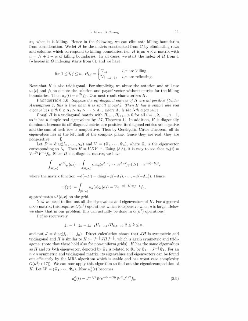
4.1. Convergence of Localization Error. Proposition 3.3 and Remark 3 showthat the localization error converges exponentially in the NIG model and the SubOUmodel, which is confirmed in our numerical experiment. In Figure 1, we plot theconvergence of localization error in these two models for a European put. For each A,we calculate the option price under the localized problem using a large number of gridpoints so that the discretization error is negligible compared to the localization error,and we can regard the difference between the approximate price and the benchmarkprice as the localization error. As discussed in Section 4.1, the finite boundaries −Aand A can be specified as either killing or reflecting. It is observed in Figure 1 that inboth specifications, the error converges exponentially, consistent with our theoreticalresult. Comparing the two specifications, using reflecting boundaries produces muchmore accurate results. This is expected, as for the original diffusion X, it is possible forit to go back to (−A,A), which is impossible when −A and A are killing boundaries.We also plot the convergence of localization error for a European put under the


A1 1.5 2 2.5

max

imum

err

or

10-6

10-5

10-4

10-3

10-2

10-1

100

NIG: KillingNIG: Reflecting

A0.6 0.7 0.8 0.9 1 1.1 1.2

max

imum

err

or

10-6

10-5

10-4

10-3

10-2

10-1

SubOU: KillingSubOU: Reflecting

Fig. 1: Convergence of localization error for a European put under the NIG andSubOU model. We plot the maximum localization error of the option price for S0

over [80, 120] in log scale.

A1.5 2 2.5 3

max

imum

err

or

10-6

10-5

10-4

10-3

10-2

10-1

100

SubCIR: Reflecting

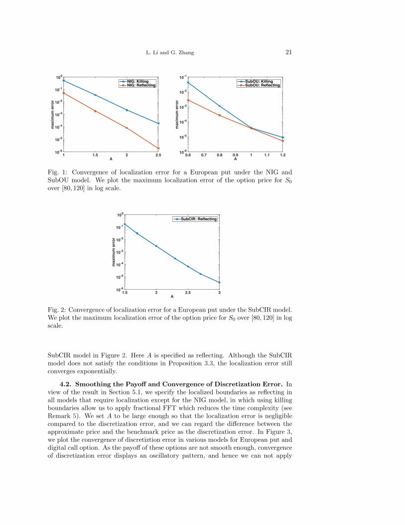
Fig. 2: Convergence of localization error for a European put under the SubCIR model.We plot the maximum localization error of the option price for S0 over [80, 120] in logscale.

SubCIR model in Figure 2. Here A is specified as reflecting. Although the SubCIRmodel does not satisfy the conditions in Proposition 3.3, the localization error stillconverges exponentially.

4.2. Smoothing the Payoff and Convergence of Discretization Error. Inview of the result in Section 5.1, we specify the localized boundaries as reflecting inall models that require localization except for the NIG model, in which using killingboundaries allow us to apply fractional FFT which reduces the time complexity (seeRemark 5). We set A to be large enough so that the localization error is negligiblecompared to the discretization error, and we can regard the difference between theapproximate price and the benchmark price as the discretization error. In Figure 3,we plot the convergence of discretiztion error in various models for European put anddigital call option. As the payoff of these options are not smooth enough, convergenceof discretization error displays an oscillatory pattern, and hence we can not apply


Richardson extrapolation to speed up convergence. We propose to use the projectionmethod in [51] to smooth the payoff (see their paper for detailed account of this ap-proach). Figure 3 shows convergence of discretization error now becomes smooth andextrapolation becomes applicable. Furthermore, the slope of the smooth line indicatesthe convergence order is two. It is interesting to note that although projection in-troduces error to the initial data, it does not necessarily make the numerical solutionless accurate. As Figure 3 shows, using projection leads to more accurate numericalsolution for pricing European put options under the subordinate reflected Brownianmotion and digital call options under the NIG model. In other cases, for a given grid,projection results in slightly larger error and in the worse case the error is three timesof the error using the original payoff. The advantage of projection is that it makesextrapolation possible so that we can obtain highly accurate solution with small gridsize, despite that for each grid, the solution under projection might be less accurate.

We next apply extrapolation to the price sequence for the projected payoff forvarious models and results for the ATM case (S0 = K) are displayed in Table 1.Extrapolation works very well in all models. By extrapolating the price in the first tworows, we already achieve a relative error around 0.01% or 0.001% in a few millisecondsin all cases! This suffices for financial applications where typically a relative error oforder 0.1% is good enough (see [8]). We have also tested the accuracy in the OTM(S0 > K) and ITM (S0 < K) case, and results are similar to the ATM case. We donot display such results here to save space.

4.3. Comparison to a PIDE Scheme for the NIG Model. For popularLevy subordinate Brownian motion models, there already exist several PIDE schemes.Here we compare our method to a very efficient PIDE scheme developed in [16] (here-after we call it DFV) for the NIG model. The DFV scheme is developed for jumpprocesses with finite activity. To apply it, we approximate the small jump part by aBrownian motion as in [14] and large jumps are also truncated. As mentioned in Re-mark 6, the DFV schemes has time complexity O(mn log2 n), where m is the numberof time steps and n is the number of grid points for the space variable. In contrast, ourmethod does not discretize time and the time complexity is O(n log2 n). Furthermore,our method does not have approximation error for small and large jumps. Figure 4compares the DFV scheme and our FDEIG method for European put option for twomaturities. We plot the maximum error and the corresponding computation time. Itis clear that for all maturities considered, the FDEIG method is faster for given levelsof accuracy. Moreover, as expected, the difference becomes more pronounced as thematurity increases.

4.4. The Option Delta. The delta of an option is important for hedging. Fora point xi in the interior of the grid, we approximate uφx(t, xi) as

uφx(t, xi) ≈uφh,i+1(t)− uφh,i−1(t)

2h,

where uφh,i±1(t) approximates uφ(t, xi±h). To calculate uφh(t), we can use the originalpayoff or the projected payoff. Figure 5 plots the convergence of delta for both payoffsunder three models. To obtain the benchmark, we use the transform approach underthe NIG model and for the SubCIR and SubJDCEV model, we use an analyticalexpression for the delta derived from the eigenfunction expansion for the price viaterm-by-term differentiation (see [40, Eq.(19)]). Like the case for option price, theconvergence is oscillatory under the original payoff but smooth under the projected


1/h101 102

max

imum

err

or

10-4

10-3

10-2

10-1

100 NIG: Putprojected payofforiginal payoff

1/h102 103

max

imum

err

or

10-5

10-4

10-3

10-2

10-1 SubRBM: Putprojected payofforiginal payoff

1/h100 101

max

imum

err

or

10-6

10-5

10-4

10-3

10-2

10-1 SubJDCEV: Putprojected payofforiginal payoff

1/h101 102

max

imum

err

or

10-5

10-4

10-3

10-2

10-1

100 SubCIR: Putprojected payofforiginal payoff

1/h101 102

max

imum

err

or

10-5

10-4

10-3

10-2

10-1

100 NIG: Digital Callprojected payofforiginal payoff

Fig. 3: Convergence of discretization error for various models (log-log scale). Weplot the maximum error of the option price for S0 over [80, 120] for the original andprojected payoff.

payoff. Furthermore, the convergence order is two in the projected payoff case. Weapply extrapolation to speed up convergence and Table 2 shows the extrapolationresults. We are able to achieve high level of accuracy for the delta in a few milliseconds.

5. Conclusions. This paper develops a novel and efficient method named asFDEIG for pricing European options in models based on one-dimensional subordi-


Time/ms100 101 102 103

max

imum

err

or

10-4

10-3

10-2

10-1T=1

DFVFDEIG

Time/ms100 101 102 103

max

imum

err

or

10-4

10-3

10-2

10-1T=5

DFVFDEIG

Fig. 4: Comparison of the DFV scheme and the FDEIG method for pricing Europeanput under the NIG model. The localization interval is set to be (−4, 4) in bothmethods. We plot the maximum error for S0 ∈ [80, 120] with the correspondingcomputation time.

1/h101 102

max

imum

err

or

10-5

10-4

10-3

10-2

10-1 NIG: Put Deltaprojected payofforiginal payoff

1/h101 102

max

imum

err

or

10-6

10-5

10-4

10-3

10-2 SubCIR: Put Deltaprojected payofforiginal payoff

1/h100 101

max

imum

err

or

10-7

10-6

10-5

10-4

10-3

10-2 SubJDCEV: Put Deltaprojected payofforiginal payoff

Fig. 5: Convergence of the delta of European put options under the NIG and SubCIR,SubJDCEV models (log-log scale). We plot the maximum error for the delta forS0 ∈ [80, 120].


NIG: PutN Projected Error Order Time/ms Extrapolated Error

128 9.528940 -3.37E-02 0.6256 9.554093 -8.54E-03 1.98 1.8 9.562478 -1.54E-04512 9.560486 -2.15E-03 1.99 2.4 9.562617 -1.49E-05

SubRBM: PutN Projected Error Order Time/ms Extrapolated Error

16 2.436106 -9.77E-03 0.232 2.443634 -2.24E-03 2.13 0.3 2.446143 2.70E-0464 2.445333 -5.39E-04 2.05 0.8 2.445899 2.70E-05

SubCIR: PutN Projected Error Order Time/ms Extrapolated Error

128 11.053394 -3.37E-02 2.2256 11.078793 -8.29E-03 2.02 6.6 11.087259 1.78E-04512 11.085021 -2.06E-03 2.01 26.5 11.087097 1.54E-05

SubJDCEV: PutN Projected Error Order Time/ms Extrapolated Error

128 1.655903 -9.71E-03 1.9256 1.663168 -2.44E-03 1.99 6.1 1.665590 -2.19E-05512 1.664999 -6.13E-04 1.99 28.5 1.665609 -2.96E-06

NIG: Digital CallN Projected Error Order Time/ms Extrapolated Error

128 0.412030 -4.97E-03 0.6256 0.415784 -1.21E-03 2.03 1.3 0.417035 3.85E-05512 0.416701 -2.96E-04 2.03 2.5 0.417006 9.41E-06

Table 1: Extrapolation results for the option price when S0 = 100. The “Projected”column shows the option price with projected payoff for various grid size N whilethe “Extrapolated” column shows the extrapolated value using the price from the“Projected” column in previous and current row. The first error column shows theerror for unextrapolated price, while the second error column shows the error for theextrapolated price. The order is defined as − log2(eN/eN/2) where eN is the error fora grid with size N . “ms” stands for milliseconds.

nate diffusions, which are obtained by time changing a one-dimensional diffusion withan independent Levy or additive subordinator. The diffusion process under consider-ation is a regular one with drift µ(x), diffusion coefficient σ(x) and killing rate k(x)and it lives on an interval with end-point l and r (−∞ ≤ l < r ≤ ∞). The bound-ary behavior can be either natural, exit, entrance or regular specified as killing andreflecting. Our method is applicable if on any compact sub-interval [a, b] ⊂ (l, r),σ(x) > 0, σ(x) ∈ C4([a, b]), µ(x) ∈ C3([a, b]), k(x) ∈ C2([a, b]) and the proposed nu-merical scheme converges if the payoff function is bounded and piecewise continuous(see Proposition 3.2 for the convergence of localization and Proposition 3.12 for theconvergence of spatial discretization; the condition for the payoff can be weakened forthe convergence of localization). Subject to further regularity conditions, we provethat the localization error converges exponentially (Proposition 3.3) and for smoothpayoffs, the discretezation error converges in second order (Proposition 3.9). Sincefinancial payoffs are typically not smooth, we apply a smoothing technique and useextrapolation to speed up convergence. The computation complexity of our method


NIG: Put DeltaN Projected Error Order Time/ms Extrapolated Error

128 -0.43645502 2.15E-03 0.7256 -0.43806513 5.39E-04 2.00 1.5 -0.43860184 1.97E-06512 -0.43847061 1.33E-04 2.02 2.5 -0.43860577 -1.96E-06

SubCIR: Put DeltaN Projected Error Order Time/ms Extrapolated Error

128 -0.39393376 -7.52E-05 2.2256 -0.39387687 -1.83E-05 2.04 7.0 -0.39385790 7.10E-07512 -0.39386314 -4.53E-06 2.01 24.1 -0.39385856 4.84E-08

SubJDCEV: Put DeltaN Projected Error Order Time/ms Extrapolated Error

128 -0.27181061 2.99E-05 1.8256 -0.27183261 7.87E-06 1.92 6.2 -0.27183994 5.37E-07512 -0.27183848 2.00E-06 1.98 28.8 -0.27184044 3.93E-08

Table 2: Extrapolation results for the option delta when S0 = 100.

is O(n2) where n is the number of grid points (excluding killing boundaries) and thecomplexity can be reduced to O(n log2 n) for subordinate Brownian motions. Com-pared to existing numerical PIDE schemes, the FDEIG method does not discretizetime and hence there is no time discretization error. Furthermore, it does not truncatelarge and small jumps, which is done in existing PIDE schemes. Various numerical ex-periments confirm the computational efficiency and accuracy of the FDEIG method.We also compare it to a popular PIDE scheme for subordinate Brownian motions andshow that it can have significant computational advantages over the existing PIDEscheme for these processes.

While we use finite difference to discretize the diffusion PDE, we remark that finiteelement can also be used, which leads us to solve some generalized matrix eigenvalueproblem in the form Hx = λMx. Compared to the finite difference case, this problemcannot be solved in O(n2) in general, thus one would expect that using the samenumber of grid points, the finite difference discretization is faster than the finiteelement method. This is the primary reason why we choose to use finite difference inthis paper. However, the finite element approach can be advantageous in that thereis no need to smooth the payoff in order to apply extrapolation and error order canbe found quite easily for general payoffs.

The current paper focuses on pricing European options. For path-dependentoptions, we expect that our method can be extended to price discretely monitoredones with backward induction, and for American options, we will extend our schemeto solve the corresponding variational inequality. In future research, we also plan toconsider how to price multivariate options in asset price models based on multivariatesubordinate diffusions that are constructed via multivariate subordination in [47].

Appendix A. Proof for Lemmas.

Proof. [Lemma 3.1] (i) A and −A are killing: Let ζ ′ := inf {t ≥ 0 : Mt,x ≥ A}.Then the lifetime of XA, ζA = min(ζ, ζ ′), where ζ is the lifetime of X (XA can bekilled either by hitting A or −A, or by the killing rate, whichever occurs first). We


also have XAs = Xs1{ζA>s} + ∆1{ζA≤s}.

uA(s, x)− u(s, x) = Ex[f(XAs )1{ζA>s}]− Ex[f(Xs)1{ζ>s}]

= Ex[f(Xs)1{ζ>s}1{ζ′>s}]− Ex[f(Xs)1{ζ>s}] = −Ex[f(Xs)1{ζ>s}1{ζ′≤s}].

Therefore |uA(s, x) − u(s, x)| ≤ Ex[f(Xs)1{Ms,x≥A}]. Under the second assumption

on f , we have |uA(s, x)− u(s, x)| ≤ ‖f‖∞ Px(Ms,x ≥ A).

(ii) A and −A are reflecting: XAs = XA

s 1{Ms,x≥A} + Xs1{Ms,x<A} for s ≥ 0 and

uA(s, x) = Ex[f(XAs )1{ζA>s}1{Ms,x<A}] + Ex[f(XA

s )1{ζA>s}1{Ms,x≥A}]

= Ex[f(XAs )1{ζA>s}1{Ms,x<A}] + Ex[f(XA

s )1{ζA>s}1{Ms,x≥A}]

= Ex[f(Xs)1{ζ>s}1{Ms,x<A}] + Ex[f(XAs )1{ζA>s}1{Ms,x≥A}].

Hence under the first assumption, we have

|uA(s, x)− u(s, x)| = | − Ex[f(Xs)1{ζ>s}1{Ms,x≥A}] + Ex[f(XAs )1{ζA>s}1{Ms,x≥A}]|

≤ Ex[f(Xs)1{Ms,x≥A}] + Ex[f(Ms,x)1{Ms,x≥A}] + Ex[f(−Ms,x)1{Ms,x≥A}],

where we used monotonicity of f to conclude that f(XAs ) is bounded by f(Ms,x) +

f(−Ms,x). Under the second assumption, |uA(s, x)−u(s, x)| ≤ 2 ‖f‖∞ Px (Ms,x ≥ A).

Proof. [Lemma 3.4] [25] proves the claim for λn and ϕ(k)n for k = 0, 1 based on

Volterra’s integral equation. We can follow this idea by taking successive differenti-

ation of the integral equation to prove the result for ϕ(k)n (k = 2, 3, 4). The detailed

proof is omitted here.Proof. [Lemma 3.7] Our assumption implies that the conditions in Theorem 5.2

of [30] are satisfied, applying which shows that for any T > 0, u ∈ H 4+ε2 ,4+ε([0, T ] ×

[l, r]). This implies that ∂xxxu(t, x), ∂xxxxu(t, x) are bounded on [0, T ]× [l, r] for anyT > 0. By the Cauchy-Schwartz inequality, |fn| ≤ ‖f‖2 for all n, where ‖f‖2 :=(∫

[l,r]f2(x)m(dx))1/2 is the L2-norm of f . This fact together with Lemma 3.4 imply

that there exists a constant C > 0 such that,

|∂xxxu(t, x)| ≤∞∑n=1

|fn| eλnt |ϕ′′′n (x)| ≤ C∞∑n=1

n3eλnt,

|∂xxxxu(t, x)| ≤∞∑n=1

|fn| eλnt |ϕ′′′′n (x)| ≤ C∞∑n=1

n4eλnt.

As t → ∞, both infinite series on the RHS tend to zero. Therefore ∂xxxu(t, x),∂xxxxu(t, x) are uniformly bounded on [0,∞)× [l, r].

Proof. [Lemma 3.7] Under our assumption, the conditions in Theorem 5.3 of [30]

are satisfied, applying which shows that for any T > 0, u ∈ H 5+ε2 ,5+ε([0, T ] × [l, r]).

Hence ∂xxxu(t, x), ∂xxxxu(t, x) and ∂t∂xxxu(t, x) are bounded on [0, T ] × [l, r]. Theuniform boundedness of ∂xxxu(t, x), ∂xxxxu(t, x) on [0,∞) × [l, r] can be derived inthe same way as Lemma 3.7. Now consider ∂t∂xxxu(t, x). Applying Cauchy-Schwartzinequality to fn and Lemma 3.4, there exists C > 0 such that

|∂t∂xxxu(t, x)| ≤∞∑n=1

|fnλn| eλnt |ϕ′′′n (x)| ≤ C∞∑n=1

n3|λn|eλnt,


As t → ∞, the infinite series on the RHS of the inequality tend to zero. Hence∂t∂xxxu(t, x) is uniformly bounded in [0,∞)× [l, r].

Proof. [Lemma 3.8] Under our assumption, the conditions in Theorem 5.3 of [30]

are satisfied, applying which shows that for any T > 0, u ∈ H 5+ε2 ,5+ε([0, T ] × [l, r]).

Hence ∂xxxu(t, x), ∂xxxxu(t, x) and ∂t∂xxxu(t, x) are bounded on [0, T ] × [l, r]. Theuniform boundedness of ∂xxxu(t, x), ∂xxxxu(t, x) on [0,∞) × [l, r] can be derived inthe same way as Lemma 3.7. Now consider ∂t∂xxxu(t, x). Applying Cauchy-Schwartzinequality to fn and Lemma 3.4, there exists C > 0 such that

|∂t∂xxxu(t, x)| ≤∞∑n=1

|fnλn| eλnt |ϕ′′′n (x)| ≤ C∞∑n=1

n3|λn|eλnt,

As t → ∞, the infinite series on the RHS of the inequality tend to zero. Hence∂t∂xxxu(t, x) is uniformly bounded in [0,∞)× [l, r].

Proof. [Lemma 3.11] We first note that there exists positive constant Cl < Cuwhich are independent of h such that

Cl ≤ ‖J‖∞ ≤ Cu. (A.1)

This can be proved following the argument in the proof of Lemma 1 in [26]. Recallthat Λk is the k-th eigenvalue of H and let Φk be the k-th normalized eigenvector(ΦTk JΦk = 1). We obtain an expression for Ps,i,j . In (3.10), setting the functionφ(λ) = λ (which corresponds to the no time change case) and fh to be a vector whosej-th element is one and all others zero, we obtain Ps,i,j = Jj,j

∑nk=1 e

ΛksΦk,iΦk,j(recall that n = N + 1−# of killing boundaries).

We will apply results from [26] and [9]. The boundary conditions for the differ-ential equation in their set-up are homogeneous Dirichlet conditions (correspondingto killing boundaries) and the finite-difference scheme they analyze is a little bit d-ifferent from ours. Nevertheless one can prove that their results still hold in ourfinite-difference scheme for both killing and reflecting boundaries by modifying thearguments in these references (we omit such lengthy discussions here). From thetheorem in [26], there is a constant C1 independent of h and k such that

‖Φk/dk‖∞ ≤ C1

√h, where dk =

√√√√ n∑i=1

Φ2k,i.

Since∑ni=1 Φ2

k,iJi,i = 1, applying (A.1), we obtain dk ≤ 1/√Cl. Therefore ‖Φk‖∞ ≤

(C1/√Cl)√h. By [9, Lemma 3], there is a positive integer k0, independent of n and

constants K1,K2, independent of h such that for k0 ≤ k ≤ n, K1k2π2 ≤ Λk ≤

K2k2π2 which implies that

∑nk=1 e

Λks ≤ (k0 − 1) +∑∞k=0 e

−K1k2π2s ≤ C2 where C2

is independent of h. Therefore

Ps,i,j ≤ maxj|Jj,j |max

k,i,j|Φk,iΦk,j |

n∑k=1

eΛks ≤ Cu(C21/Cl)C2h.

By Lemma 3.4, for all k, ‖ϕk‖∞ is bounded by a constant. We also have λk ∼O(−k2), so

∑∞k=1 e

λks is also bounded by some constant. From [45], p(s, x, y) =

m(y)∑∞k=1 e

λksϕk(x)ϕk(y). Hence sup(x,y)∈(l,r)×(l,r) p(s, x, y) ≤ ‖m‖∞ ‖ϕk‖2∞∑∞k=1 e

λks,which is bounded by some constant (the speed density m is continuous on [l, r] andhence bounded).


REFERENCES

[1] Andersen, L. and Andreasen, J., Jump-diffusion processes: volatility smile fitting and nu-merical methods for option pricing, Review of Derivatives Research, 4 (2000), pp. 231–262.

[2] Barndorff-Nielsen, O. E., Processes of Normal Inverse Gaussian type, Finance and Stochas-tics, 2 (1998), pp. 41–68.

[3] Barndorff-Nielsen, O. E. and Levendorskii, S., Feller processes of Normal Inverse Guas-sian type, Quantitative Finance, 1 (2001), pp. 318–331.

[4] Borodin, A. and Salminen, P., Handbook of Brownian Motion—Facts and Formulae,Birkhauser, Basel, 2nd ed., 2002.

[5] Boyarchenko, N. and Levendorskii, S., The eigenfunction expansion method in multifactorquadratic term structure models, Mathematical Finance, 17 (2007), pp. 503–539.

[6] Boyarchenko, S. and Levendorskii, S., Non-Gaussian Merton-Black-Scholes Theory, vol. 9,World Scientific, 2002.

[7] Boyarchenko, S. and Levendorskii, S., New efficient versions of Fourier transform methodin applications to option pricing, Journal of Computational Finance, (2013).

[8] Broadie, M. and Detemple, J. B., American option valuations: new bounds, approximations,and a comparison of existing methods, Review of Financial Studies, 9 (1996), pp. 1211–1250.

[9] Carasso, A., Finite-difference methods and the eigenvalue problem for nonselfadjoint Sturm-Liouville operators, Mathematics of Computation, 23 (1969), pp. 717–729.

[10] Carr, P. and Linetsky, V., A jump to default extended CEV model: an application of Besselprocesses, Finance and Stochastics, 10 (2006), pp. 303–330.

[11] Carr, P. and Madan, D. B., Option valuation using the fast Fourier transform, Journal ofComputational Finance, 2 (1999), pp. 61–73.

[12] Conley, T. G., Hansen, L. P., Luttmer, E. G. J., and Scheinkman, J. A., Short-terminterest rates as subordinated diffusions, Review of Financial Studies, 10 (1997), pp. 525–577.

[13] Cont, R. and Tankov, P., Financial Modeling with Jump Processes, Chapman & Hall, Cam-bridge, 2004.

[14] Cont, R. and Voltchkova, E., A finite difference scheme for option pricing in jump diffusionand exponential Levy models, SIAM Journal on Numerical Analysis, 43 (2005), pp. 1596–1626.

[15] Cont, R. and Voltchkova, E., Integro-differential equations for option prices in exponentialLevy models, Finance and Stochastics, 9 (2005), pp. 299–325.

[16] d’Halluin, Y., Forsyth, P., and Vetzal, K., Robust numerical methods for contingentclaims under jump diffusion processes, IMA Journal on Numerical Analysis, 25 (2005),pp. 87–112.

[17] Dhillon, I. S., A new O(n2) Algorithm for the Symmetric Tridiagonal Eigenvalue/EigenvectorProblem, PhD thesis, The University of California at Berkeley, 1997.

[18] Dixit, A. K. and Pindyck, R. S., Investment Under Uncertainty, Princeton University Press,Princeton, NJ, 1994.

[19] Ekstrom, E. and Tysk, J., Boundary conditions for the single-factor term structure equation,The Annals of Applied Probability, 21 (2011), pp. 332–350.

[20] Fang, F. and Oosterlee, C. W., A novel pricing method for european options based onFourier-cosine series expansions, SIAM Journal on Scientific Computing, 31 (2008), p-p. 826–848.

[21] , Pricing early-exercise and discrete barrier options by Fourier-cosine series expansions,Numerische Mathematik, 114 (2009), pp. 27–62.

[22] Feng, L. and Linetsky, V., Pricing discretely monitored barrier options and defaultable bondsin Levy process models: a fast Hilbert transform approach, Mathematical Finance, 18(2008), pp. 337–384.

[23] , Pricing options in jump-diffusion models: an extrapolation approach, Operations Re-search, 56 (2008), pp. 304–325.

[24] , Computing exponential moments of the discrete maximum of a Levy process and look-back options, Finance and Stochastics, 13 (2009), pp. 501–529.

[25] Fulton, C. T. and Pruess, S. A., Eigenvalue and eigenfunction asymptotics for regularsturm-liouville problems, Journal of Mathematical Analysis and Applications, 188 (1994),pp. 297–340.

[26] Gekeler, E., On the eigenvectors of a finite-difference approximation to the Sturm-Liouvilleeigenvalue problem, Mathematics of Computation, (1974), pp. 973–979.

[27] Heston, S. and Zhou, G., On the rate of convergence of discrete-time contingent claims,


Mathematical Finance, 10 (2000), pp. 53–75.[28] Karlin, S. and Taylor, H. M., A Second Course in Stochastic Processes, Academic Press,

New York, 1981.[29] Knight, F. B., Essentials of Brownian Motion and Diffusion, vol. 18 of Mathematical Surveys

and Monographs, American Mathematical Society, Providence, 1981.[30] Ladyzhenskaia, O. A., Solonnikov, V. A., and Ural’tseva, N. N., Linear and quasi-linear

equations of parabolic type, vol. 23, American Mathematical Soc., 1988.[31] Lessig, C. and Bientinesi, P., On parallelizing the mrrr algorithm for data-parallel coproces-

sors, in Parallel Processing and Applied Mathematics, Springer, 2010, pp. 396–402.[32] Li, J., Li, L., and Mendoza-Arriaga, R., Additive subordination and its applications in

finance, Finance and Stochastics, (2016). Forthcoming.[33] Li, J., Li, L., and Zhang, G., A pure jump model for pricing and hedging VIX options, (2015).

Working paper.[34] Li, L. and Linetsky, V., Optimal stopping and early exercise: an eigenfunction expansion

approach, Operations Research, 61 (2013), pp. 625–643.[35] , Optimal stopping in infinite horizon: an eigenfunction expansion approach, Statistics

and Probability Letters, 85 (2014), pp. 122–128.[36] , Time-changed Ornstein-Uhlenbeck processes and their applications in commodity

derivative models, Mathematical Finance, 24 (2014), pp. 289–330.[37] , Discretely monitored first passage problems and barrier options: an eigenfunction ex-

pansion approach, Finance and Stochastics, 19 (2015), pp. 941–977. DOI 10.1007/s00780-015-0271-1.

[38] Li, L. and Mendoza, R., Ornstein-Uhlenbeck processes time-changed with additive subordina-tors and their applications in commodity derivative models, Operations Research Letters,41 (2013), pp. 521–525.

[39] Li, L., Mendoza-Arriaga, R., Mo, Z., and Mitchell, D., Modelling electrici-ty prices: a time change approach, Quantitative Finance, (2016). available athttp://dx.doi.org/10.1080/14697688.2015.1125521.

[40] Li, L., Qu, X., and Zhang, G., An efficient algorithm based on eigenfunction expansion-s for some optimal timing problems in finance, Journal of Computational and AppliedMathematics, 294 (2016), pp. 225–250.

[41] Lim, D., Li, L., and Linetsky, V., Evaluating callable and putable bonds: an eigenfunctionexpansion approach, Journal of Economic Dynamics and Control, 36 (2012), pp. 1888–1908.

[42] Linetsky, V., Spectral methods in derivatives pricing, in Handbook of Financial Engineering,Handbooks in Operations Research and Management Sciences, Birge, J. R. and Linetsky,V., eds., Elsevier, 2008, ch. 6.

[43] Lord, R., Fang, F., Bervoets, F., and Oosterlee, C. W., A fast and accurate FFT-basedmethod for pricing early-exercise options under Levy processes, SIAM Journal on ScientificComputing, 30 (2008), pp. 1678–1705.

[44] Madan, D. and Yor, M., Representing the CGMY and Meixner Levy processes as timechanged Brownian motions, Journal of Computational Finance, 12 (2008), pp. 27–47.

[45] McKean, H. P., Elementary Solutions for Certain Parabolic Partial Differential Equations,Transactions of the American Mathematical Society, 82 (1956), pp. 519–548.

[46] Mendoza-Arriaga, R., Carr, P., and Linetsky, V., Time changed Markov processes inunified credit-equity modeling, Mathematical Finance, 20 (2010), pp. 527–569.

[47] Mendoza-Arriaga, R. and Linetsky, V., Multivariate subordination of Markov processeswith financial applications, Mathematical Finance, (2014). Ariticle published online.

[48] , Time-changed CIR default intensities with two-sided mean-reverting jumps, The Annalsof Applied Probability, 24 (2014), pp. 811–856.

[49] Oleinik, O. A. and Radkevic, E. V., Second-order equations with nonnegative characteristicform, Plenum Press, 1973.

[50] Pascucci, A., PDE and Martingale Methods in Option Pricing, Springer, 2011.[51] Pooley, D. M., Vetzal, K. R., and Forsyth, P. A., Convergence remedies for non-smooth

payoffs in option pricing, Journal of Computational Finance, 6 (2003), pp. 25–40.[52] Rong, S., On solutions of backward stochastic differential equations with jumps and applica-

tions, Stochastic Processes and their Applications, 66 (1997), pp. 209–236.[53] Sato, K., Levy Processes and Infinitely Divisible Distributions, Cambidge University Press,

1999.[54] Schilling, R. L., Song, R., and Vondracek, Z., Bernstein Functions: Theory and Applica-

tions, no. 37 in De Gruyter studies in mathematics, De Gruyter, Berlin, 2nd. ed., 2012.[55] Thomee, V. and Wahlbin, L., Convergence rates of parabolic difference schemes for non-

smooth data, Mathematics of Computation, 28 (1974), pp. 1–13.


[56] Todorov, V. and Tauchen, G., Volatility jumps, Journal of Business & Economic Statistics,29 (2011), pp. 356–371.

[57] Veselic, K., On real eigenvalues of real tridiagonal matrices, Linear Algebra and its Applica-tions, 27 (1979), pp. 167–171.

[58] Yueh, W.-C., Eigenvalues of several tridiagonal matrices, Applied Mathematics E-Notes, 5(2005), pp. 210–230.

option pricing in some non-lévy jump models

Documents

Transcript of option pricing in some non-lévy jump models