MIKE ZERO PREPROCESSING & POSTPROCESSING

MIKE ZEROPREPROCESSING &POSTPROCESSING

Volume 1 - Generic Editors and Viewers

User Guides

MIKE by DHI 2014

Please Note

CopyrightThis document refers to proprietary computer software which is protectedby copyright. All rights are reserved. Copying or other reproduction ofthis manual or the related programs is prohibited without prior writtenconsent of DHI. For details please refer to your 'DHI Software LicenceAgreement'.

Limited LiabilityThe liability of DHI is limited as specified in Section III of your 'DHISoftware Licence Agreement':

'IN NO EVENT SHALL DHI OR ITS REPRESENTATIVES (AGENTSAND SUPPLIERS) BE LIABLE FOR ANY DAMAGES WHATSO-EVER INCLUDING, WITHOUT LIMITATION, SPECIAL, INDIRECT,INCIDENTAL OR CONSEQUENTIAL DAMAGES OR DAMAGESFOR LOSS OF BUSINESS PROFITS OR SAVINGS, BUSINESSINTERRUPTION, LOSS OF BUSINESS INFORMATION OR OTHERPECUNIARY LOSS ARISING OUT OF THE USE OF OR THE INA-BILITY TO USE THIS DHI SOFTWARE PRODUCT, EVEN IF DHIHAS BEEN ADVISED OF THE POSSIBILITY OF SUCH DAMAGES.THIS LIMITATION SHALL APPLY TO CLAIMS OF PERSONALINJURY TO THE EXTENT PERMITTED BY LAW. SOME COUN-TRIES OR STATES DO NOT ALLOW THE EXCLUSION OR LIMITA-TION OF LIABILITY FOR CONSEQUENTIAL, SPECIAL, INDIRECT,INCIDENTAL DAMAGES AND, ACCORDINGLY, SOME PORTIONSOF THESE LIMITATIONS MAY NOT APPLY TO YOU. BY YOUROPENING OF THIS SEALED PACKAGE OR INSTALLING ORUSING THE SOFTWARE, YOU HAVE ACCEPTED THAT THEABOVE LIMITATIONS OR THE MAXIMUM LEGALLY APPLICA-BLE SUBSET OF THESE LIMITATIONS APPLY TO YOUR PUR-CHASE OF THIS SOFTWARE.'

Printing HistoryJune 2003June 2004June 2005December 2006November 2007January 2009November 2010September 2012November 2013

3

4 MIKE Zero

C O N T E N T S

5

Time Series Editor . . . . . . . . . . . . . . . . . . . . . . . . . . . . . . . . . . . . 17

1 TIME SERIES EDITOR . . . . . . . . . . . . . . . . . . . . . . . . . . . . . . . . 191.1 Introduction . . . . . . . . . . . . . . . . . . . . . . . . . . . . . . . . . . . 191.2 New File Dialog . . . . . . . . . . . . . . . . . . . . . . . . . . . . . . . . . 19

1.2.1 Import from ASCII File . . . . . . . . . . . . . . . . . . . . . . . . 201.2.2 Wave Climate Template . . . . . . . . . . . . . . . . . . . . . . . 221.2.3 LITProf template . . . . . . . . . . . . . . . . . . . . . . . . . . . . 231.2.4 LITTren template . . . . . . . . . . . . . . . . . . . . . . . . . . . 241.2.5 Source Template . . . . . . . . . . . . . . . . . . . . . . . . . . . 251.2.6 STPBatch template . . . . . . . . . . . . . . . . . . . . . . . . . . 251.2.7 Wind template . . . . . . . . . . . . . . . . . . . . . . . . . . . . . 26

1.3 Export to ASCII File . . . . . . . . . . . . . . . . . . . . . . . . . . . . . . . 261.4 File Properties Dialog . . . . . . . . . . . . . . . . . . . . . . . . . . . . . . 27

1.4.1 General Information . . . . . . . . . . . . . . . . . . . . . . . . . . 271.4.2 Axis Information . . . . . . . . . . . . . . . . . . . . . . . . . . . . 271.4.3 Item Information . . . . . . . . . . . . . . . . . . . . . . . . . . . . 28

1.5 Tabular View . . . . . . . . . . . . . . . . . . . . . . . . . . . . . . . . . . . 301.6 Graphical View . . . . . . . . . . . . . . . . . . . . . . . . . . . . . . . . . 31

1.6.1 Zoom . . . . . . . . . . . . . . . . . . . . . . . . . . . . . . . . . . 311.6.2 Editing modes . . . . . . . . . . . . . . . . . . . . . . . . . . . . . 311.6.3 Graphical and font settings . . . . . . . . . . . . . . . . . . . . . . 321.6.4 TS Types graphical representation . . . . . . . . . . . . . . . . . 33

1.7 Graphical Settings Dialog . . . . . . . . . . . . . . . . . . . . . . . . . . . 331.8 Font Settings Dialog . . . . . . . . . . . . . . . . . . . . . . . . . . . . . . 341.9 File Formats . . . . . . . . . . . . . . . . . . . . . . . . . . . . . . . . . . . 341.10 Tools . . . . . . . . . . . . . . . . . . . . . . . . . . . . . . . . . . . . . . . 36

1.10.1 Calculator . . . . . . . . . . . . . . . . . . . . . . . . . . . . . . . 361.10.2 Interpolation . . . . . . . . . . . . . . . . . . . . . . . . . . . . . . 371.10.3 Select Sub-Set . . . . . . . . . . . . . . . . . . . . . . . . . . . . . 381.10.4 Statistics . . . . . . . . . . . . . . . . . . . . . . . . . . . . . . . . 391.10.5 Edit Custom Blocks . . . . . . . . . . . . . . . . . . . . . . . . . . 40

Profile Series Editor . . . . . . . . . . . . . . . . . . . . . . . . . . . . . . . . . . . 41

2 INTRODUCTION . . . . . . . . . . . . . . . . . . . . . . . . . . . . . . . . . . . . 432.1 Create a New Dataset . . . . . . . . . . . . . . . . . . . . . . . . . . . . . 432.2 Open an Existing Dataset . . . . . . . . . . . . . . . . . . . . . . . . . . . 432.3 Editing the Dataset . . . . . . . . . . . . . . . . . . . . . . . . . . . . . . . 432.4 Further help . . . . . . . . . . . . . . . . . . . . . . . . . . . . . . . . . . . 44

3 PROPERTIES . . . . . . . . . . . . . . . . . . . . . . . . . . . . . . . . . . . . . . 453.1 New Profile Series Dialog . . . . . . . . . . . . . . . . . . . . . . . . . . . 45

6 MIKE Zero

3.1.1 Cross-shore profile . . . . . . . . . . . . . . . . . . . . . . . . . . 463.1.2 Initial coastline alignment . . . . . . . . . . . . . . . . . . . . . . . 463.1.3 Cross-section of Trench . . . . . . . . . . . . . . . . . . . . . . . 473.1.4 Pier Resistance Profile . . . . . . . . . . . . . . . . . . . . . . . . 483.1.5 ADCP Vector Plot . . . . . . . . . . . . . . . . . . . . . . . . . . . 49

3.2 Geographical Information . . . . . . . . . . . . . . . . . . . . . . . . . . . . 503.3 File Properties Dialog . . . . . . . . . . . . . . . . . . . . . . . . . . . . . . 50

3.3.1 General Information . . . . . . . . . . . . . . . . . . . . . . . . . . 503.3.2 Axis Information . . . . . . . . . . . . . . . . . . . . . . . . . . . . 513.3.3 Item Information . . . . . . . . . . . . . . . . . . . . . . . . . . . . 51

3.4 Tabular View . . . . . . . . . . . . . . . . . . . . . . . . . . . . . . . . . . . 523.4.1 Cell format . . . . . . . . . . . . . . . . . . . . . . . . . . . . . . . 53

3.5 Graphical View . . . . . . . . . . . . . . . . . . . . . . . . . . . . . . . . . . 533.5.1 Zoom . . . . . . . . . . . . . . . . . . . . . . . . . . . . . . . . . . 533.5.2 Graphical and font settings . . . . . . . . . . . . . . . . . . . . . . 54

3.6 Navigation View . . . . . . . . . . . . . . . . . . . . . . . . . . . . . . . . . 543.7 File Formats . . . . . . . . . . . . . . . . . . . . . . . . . . . . . . . . . . . 54

3.7.1 DFS . . . . . . . . . . . . . . . . . . . . . . . . . . . . . . . . . . . 553.7.2 ASCII . . . . . . . . . . . . . . . . . . . . . . . . . . . . . . . . . . 55

3.8 Import from ASCII File . . . . . . . . . . . . . . . . . . . . . . . . . . . . . 563.8.1 File to Import . . . . . . . . . . . . . . . . . . . . . . . . . . . . . . 573.8.2 Completion and Editing . . . . . . . . . . . . . . . . . . . . . . . . 57

3.9 Export to ASCII File . . . . . . . . . . . . . . . . . . . . . . . . . . . . . . . 57

4 TOOLS . . . . . . . . . . . . . . . . . . . . . . . . . . . . . . . . . . . . . . . . . . 594.1 Calculator . . . . . . . . . . . . . . . . . . . . . . . . . . . . . . . . . . . . . 59

4.1.1 Edit Expression . . . . . . . . . . . . . . . . . . . . . . . . . . . . 594.1.2 Sub set . . . . . . . . . . . . . . . . . . . . . . . . . . . . . . . . . 60

4.2 Interpolation . . . . . . . . . . . . . . . . . . . . . . . . . . . . . . . . . . . 604.2.1 Gap filling . . . . . . . . . . . . . . . . . . . . . . . . . . . . . . . . 604.2.2 Sub-set . . . . . . . . . . . . . . . . . . . . . . . . . . . . . . . . . 61

4.3 Edit Custom Blocks . . . . . . . . . . . . . . . . . . . . . . . . . . . . . . . 61

Grid Series Editor . . . . . . . . . . . . . . . . . . . . . . . . . . . . . . . . . . . . . 63

5 INTRODUCTION . . . . . . . . . . . . . . . . . . . . . . . . . . . . . . . . . . . . 655.1 Create a New Dataset . . . . . . . . . . . . . . . . . . . . . . . . . . . . . 655.2 Open an Existing Dataset . . . . . . . . . . . . . . . . . . . . . . . . . . . 665.3 Editing the Dataset . . . . . . . . . . . . . . . . . . . . . . . . . . . . . . . 665.4 Further help . . . . . . . . . . . . . . . . . . . . . . . . . . . . . . . . . . . 66

7

6 FILE . . . . . . . . . . . . . . . . . . . . . . . . . . . . . . . . . . . . . . . . . . . 696.1 File Formats . . . . . . . . . . . . . . . . . . . . . . . . . . . . . . . . . . . 69

6.1.1 DFS format . . . . . . . . . . . . . . . . . . . . . . . . . . . . . . . 696.1.2 ASCII format . . . . . . . . . . . . . . . . . . . . . . . . . . . . . . 696.1.3 Grid State Format . . . . . . . . . . . . . . . . . . . . . . . . . . . 70

6.2 New Grid Series File . . . . . . . . . . . . . . . . . . . . . . . . . . . . . . 716.2.1 Step 1: Select the type of grid to be created . . . . . . . . . . . . 716.2.2 Step 2: Specify the projection, the geographical position of the origin

of the dataset and the orientation 716.2.3 Step 3: Specify the temporal and spatial properties . . . . . . . 726.2.4 Step 4: Specify the items to be included . . . . . . . . . . . . . . 736.2.5 Step 5: Overview . . . . . . . . . . . . . . . . . . . . . . . . . . . 73

6.3 Import from ASCII File . . . . . . . . . . . . . . . . . . . . . . . . . . . . . 736.3.1 File to Import . . . . . . . . . . . . . . . . . . . . . . . . . . . . . . 736.3.2 Completion and Editing . . . . . . . . . . . . . . . . . . . . . . . . 746.3.3 Hint . . . . . . . . . . . . . . . . . . . . . . . . . . . . . . . . . . . 74

6.4 Export to ASCII File . . . . . . . . . . . . . . . . . . . . . . . . . . . . . . . 746.5 Import from Dfsu File . . . . . . . . . . . . . . . . . . . . . . . . . . . . . . 74

6.5.1 Step 1: Select File to Import . . . . . . . . . . . . . . . . . . . . . 746.5.2 Step 2: Specify geographical parameters . . . . . . . . . . . . . 746.5.3 Step 3: Specify the spatial properties . . . . . . . . . . . . . . . . 756.5.4 Step 4: Specify land value . . . . . . . . . . . . . . . . . . . . . . 756.5.5 Step 5: Completion and Editing . . . . . . . . . . . . . . . . . . . 756.5.6 Step 6: Modifying Custom Block . . . . . . . . . . . . . . . . . . 75

7 EDIT . . . . . . . . . . . . . . . . . . . . . . . . . . . . . . . . . . . . . . . . . . . 777.1 Geographical Information . . . . . . . . . . . . . . . . . . . . . . . . . . . 777.2 Time Steps . . . . . . . . . . . . . . . . . . . . . . . . . . . . . . . . . . . . 77

7.2.1 Modifying Time Steps . . . . . . . . . . . . . . . . . . . . . . . . . 777.3 Items . . . . . . . . . . . . . . . . . . . . . . . . . . . . . . . . . . . . . . . 78

7.3.1 Editing an existing file . . . . . . . . . . . . . . . . . . . . . . . . 797.4 Spatial Axis . . . . . . . . . . . . . . . . . . . . . . . . . . . . . . . . . . . 807.5 Edit Custom Blocks . . . . . . . . . . . . . . . . . . . . . . . . . . . . . . . 80

7.5.1 MIKE 21 / MIKE 3 specific . . . . . . . . . . . . . . . . . . . . . . 80

8 VIEW . . . . . . . . . . . . . . . . . . . . . . . . . . . . . . . . . . . . . . . . . . . 818.1 Tabular View . . . . . . . . . . . . . . . . . . . . . . . . . . . . . . . . . . . 818.2 Graphical View . . . . . . . . . . . . . . . . . . . . . . . . . . . . . . . . . 828.3 Palette . . . . . . . . . . . . . . . . . . . . . . . . . . . . . . . . . . . . . . 828.4 Overlay . . . . . . . . . . . . . . . . . . . . . . . . . . . . . . . . . . . . . . 83

8.4.1 Map Projection . . . . . . . . . . . . . . . . . . . . . . . . . . . . . 838.4.2 North Arrow . . . . . . . . . . . . . . . . . . . . . . . . . . . . . . 83

8 MIKE Zero

8.5 Grid Settings . . . . . . . . . . . . . . . . . . . . . . . . . . . . . . . . . . . 848.6 Axis Annotation . . . . . . . . . . . . . . . . . . . . . . . . . . . . . . . . . 848.7 Mouse Pointer Coordinates . . . . . . . . . . . . . . . . . . . . . . . . . . 848.8 Fixed aspect ratio . . . . . . . . . . . . . . . . . . . . . . . . . . . . . . . . 848.9 Export Graphics . . . . . . . . . . . . . . . . . . . . . . . . . . . . . . . . . 848.10 Toolbars . . . . . . . . . . . . . . . . . . . . . . . . . . . . . . . . . . . . . 84

8.10.1 Grid Editor Tools . . . . . . . . . . . . . . . . . . . . . . . . . . . . 858.10.2 Grid Editor Navigation . . . . . . . . . . . . . . . . . . . . . . . . . 85

8.11 Status Bar . . . . . . . . . . . . . . . . . . . . . . . . . . . . . . . . . . . . 86

9 TOOLS . . . . . . . . . . . . . . . . . . . . . . . . . . . . . . . . . . . . . . . . . . 879.1 Navigation . . . . . . . . . . . . . . . . . . . . . . . . . . . . . . . . . . . . 879.2 Go to . . . . . . . . . . . . . . . . . . . . . . . . . . . . . . . . . . . . . . . 879.3 Synchronize . . . . . . . . . . . . . . . . . . . . . . . . . . . . . . . . . . . 879.4 Selection . . . . . . . . . . . . . . . . . . . . . . . . . . . . . . . . . . . . . 88

9.4.1 Select and deselect . . . . . . . . . . . . . . . . . . . . . . . . . . 889.4.2 Select a Sub-Set of Data . . . . . . . . . . . . . . . . . . . . . . . 89

9.5 Interpolation . . . . . . . . . . . . . . . . . . . . . . . . . . . . . . . . . . . 909.5.1 Active Dataset . . . . . . . . . . . . . . . . . . . . . . . . . . . . . 909.5.2 Interpolation Settings . . . . . . . . . . . . . . . . . . . . . . . . . 909.5.3 Search Type . . . . . . . . . . . . . . . . . . . . . . . . . . . . . . 90

9.6 Filter . . . . . . . . . . . . . . . . . . . . . . . . . . . . . . . . . . . . . . . . 919.7 Set Value . . . . . . . . . . . . . . . . . . . . . . . . . . . . . . . . . . . . . 919.8 Calculator . . . . . . . . . . . . . . . . . . . . . . . . . . . . . . . . . . . . . 92

9.8.1 List of Functions . . . . . . . . . . . . . . . . . . . . . . . . . . . . 929.9 Calculate Statistics . . . . . . . . . . . . . . . . . . . . . . . . . . . . . . . 959.10 Copy File into Data . . . . . . . . . . . . . . . . . . . . . . . . . . . . . . . 95

9.10.1 File to Copy . . . . . . . . . . . . . . . . . . . . . . . . . . . . . . . 969.10.2 Item Mapping . . . . . . . . . . . . . . . . . . . . . . . . . . . . . . 969.10.3 2D to 3D Layer Mapping . . . . . . . . . . . . . . . . . . . . . . . 969.10.4 Sub-area Position . . . . . . . . . . . . . . . . . . . . . . . . . . . 979.10.5 Time Position . . . . . . . . . . . . . . . . . . . . . . . . . . . . . . 979.10.6 Operation . . . . . . . . . . . . . . . . . . . . . . . . . . . . . . . . 97

9.11 Crop . . . . . . . . . . . . . . . . . . . . . . . . . . . . . . . . . . . . . . . . 97

10 DATA OVERLAY . . . . . . . . . . . . . . . . . . . . . . . . . . . . . . . . . . . . 9910.1 Image Manager . . . . . . . . . . . . . . . . . . . . . . . . . . . . . . . . . 9910.2 Overlay Manager . . . . . . . . . . . . . . . . . . . . . . . . . . . . . . . . 99

9

Bathymetry Editor . . . . . . . . . . . . . . . . . . . . . . . . . . . . . . . . . . . . 101

11 INTRODUCTION . . . . . . . . . . . . . . . . . . . . . . . . . . . . . . . . . . . . 103

12 GETTING STARTED . . . . . . . . . . . . . . . . . . . . . . . . . . . . . . . . . . 10512.1 Step 1: Create a new Bathymetry document . . . . . . . . . . . . . . . . 10512.2 Step 2: Import background data . . . . . . . . . . . . . . . . . . . . . . . . 10612.3 Step 3: Import digitised survey depth data . . . . . . . . . . . . . . . . . . 10612.4 Step 4: Import data from background . . . . . . . . . . . . . . . . . . . . 10612.5 Case A - Create Grid Bathymetry . . . . . . . . . . . . . . . . . . . . . . . 107

12.5.1 Step 5A: Define grid bathymetry . . . . . . . . . . . . . . . . . . 10712.5.2 Step 6A: Interpolate xyz data to grid points . . . . . . . . . . . . 10712.5.3 Step 7A: Save bathymetry file . . . . . . . . . . . . . . . . . . . . 107

12.6 Case B - Create Line Bathymetry . . . . . . . . . . . . . . . . . . . . . . . 10812.6.1 Step 5B: Define line bathymetry . . . . . . . . . . . . . . . . . . . 10812.6.2 Step 6B: Interpolate xyz data to grid points . . . . . . . . . . . . 10912.6.3 Step 7B: Save bathymetry file . . . . . . . . . . . . . . . . . . . . 109

13 DIALOG OVERVIEW . . . . . . . . . . . . . . . . . . . . . . . . . . . . . . . . . . 11113.1 File Menu . . . . . . . . . . . . . . . . . . . . . . . . . . . . . . . . . . . . 111

13.1.1 File/New Menu . . . . . . . . . . . . . . . . . . . . . . . . . . . . . 11113.1.2 File/Open Menu . . . . . . . . . . . . . . . . . . . . . . . . . . . . 113

13.2 Edit Menu . . . . . . . . . . . . . . . . . . . . . . . . . . . . . . . . . . . . 11413.3 View Menu . . . . . . . . . . . . . . . . . . . . . . . . . . . . . . . . . . . . 11413.4 Work Area Menu . . . . . . . . . . . . . . . . . . . . . . . . . . . . . . . . 115

13.4.1 Set Current Contour Level . . . . . . . . . . . . . . . . . . . . . . 11513.4.2 Grid Bathymetry Management . . . . . . . . . . . . . . . . . . . . 11513.4.3 Line Bathymetry Management . . . . . . . . . . . . . . . . . . . . 11613.4.4 Background Management . . . . . . . . . . . . . . . . . . . . . . 11713.4.5 Export raw data to XYZ format . . . . . . . . . . . . . . . . . . . 11913.4.6 Resize workspace area . . . . . . . . . . . . . . . . . . . . . . . . 11913.4.7 Settings . . . . . . . . . . . . . . . . . . . . . . . . . . . . . . . . . 11913.4.8 Set Font . . . . . . . . . . . . . . . . . . . . . . . . . . . . . . . . 12013.4.9 Show Background Images . . . . . . . . . . . . . . . . . . . . . . 120

13.5 Grid Bathymetry . . . . . . . . . . . . . . . . . . . . . . . . . . . . . . . . . 12013.5.1 New Bathymetry . . . . . . . . . . . . . . . . . . . . . . . . . . . . 12013.5.2 Edit Bathymetry . . . . . . . . . . . . . . . . . . . . . . . . . . . . 12413.5.3 Export Bathymetry . . . . . . . . . . . . . . . . . . . . . . . . . . 12413.5.4 Interpolate Bathymetry . . . . . . . . . . . . . . . . . . . . . . . . 124

13.6 Line Bathymetry . . . . . . . . . . . . . . . . . . . . . . . . . . . . . . . . . 12613.6.1 New bathymetry . . . . . . . . . . . . . . . . . . . . . . . . . . . . 12613.6.2 Edit bathymetry . . . . . . . . . . . . . . . . . . . . . . . . . . . . 12913.6.3 Export bathymetry . . . . . . . . . . . . . . . . . . . . . . . . . . . 12913.6.4 Interpolate bathymetry . . . . . . . . . . . . . . . . . . . . . . . . 129

10 MIKE Zero

13.7 Window Menu . . . . . . . . . . . . . . . . . . . . . . . . . . . . . . . . . 12913.8 ToolBar Functions . . . . . . . . . . . . . . . . . . . . . . . . . . . . . . . 130

Mesh Generator . . . . . . . . . . . . . . . . . . . . . . . . . . . . . . . . . . . . . 133

14 INTRODUCTION . . . . . . . . . . . . . . . . . . . . . . . . . . . . . . . . . . . 13514.1 Concepts . . . . . . . . . . . . . . . . . . . . . . . . . . . . . . . . . . . . 13614.2 Boundary Definitions . . . . . . . . . . . . . . . . . . . . . . . . . . . . . 13714.3 Context sensitive menu . . . . . . . . . . . . . . . . . . . . . . . . . . . . 138

15 GETTING STARTED . . . . . . . . . . . . . . . . . . . . . . . . . . . . . . . . . 13915.1 Introduction . . . . . . . . . . . . . . . . . . . . . . . . . . . . . . . . . . . 13915.2 Data Location . . . . . . . . . . . . . . . . . . . . . . . . . . . . . . . . . 13915.3 Step 1 - Create a New Mesh Generator Workspace . . . . . . . . . . . 13915.4 Step 2 - Import Model Boundaries . . . . . . . . . . . . . . . . . . . . . . 14015.5 Step 3 - Editing the Land Boundary . . . . . . . . . . . . . . . . . . . . . 14315.6 Step 4 - Specification of Domain . . . . . . . . . . . . . . . . . . . . . . 14615.7 Step 5 - Specification of Boundaries . . . . . . . . . . . . . . . . . . . . 14715.8 Step 6 - Mesh Generation . . . . . . . . . . . . . . . . . . . . . . . . . . 14815.9 Step 7 - Smooth the Land Boundary . . . . . . . . . . . . . . . . . . . . 15015.10 Step 8 - Smoothing the Mesh . . . . . . . . . . . . . . . . . . . . . . . . 15215.11 Step 9 - Interpolation of a Bathymetry to the Mesh . . . . . . . . . . . . 15315.12 Step 10 - Using Polygons to Control the Node Density . . . . . . . . . . 15615.13 Step 11 - Using Polygons to Define Mesh Resolution Type . . . . . . . 15915.14 Step 12 - Analyse the mesh . . . . . . . . . . . . . . . . . . . . . . . . . 162

16 REFERENCE GUIDE . . . . . . . . . . . . . . . . . . . . . . . . . . . . . . . . . 16516.1 File Menu . . . . . . . . . . . . . . . . . . . . . . . . . . . . . . . . . . . . 16516.2 Edit Menu . . . . . . . . . . . . . . . . . . . . . . . . . . . . . . . . . . . . 165

16.2.1 Undo . . . . . . . . . . . . . . . . . . . . . . . . . . . . . . . . . . 16516.2.2 Redo . . . . . . . . . . . . . . . . . . . . . . . . . . . . . . . . . . 16516.2.3 Delete . . . . . . . . . . . . . . . . . . . . . . . . . . . . . . . . . 16616.2.4 Options . . . . . . . . . . . . . . . . . . . . . . . . . . . . . . . . 166

16.3 View Menu . . . . . . . . . . . . . . . . . . . . . . . . . . . . . . . . . . . 16616.3.1 Coordinate Overlays . . . . . . . . . . . . . . . . . . . . . . . . 16616.3.2 Zoom facilities . . . . . . . . . . . . . . . . . . . . . . . . . . . . 16616.3.3 Go To . . . . . . . . . . . . . . . . . . . . . . . . . . . . . . . . . 16716.3.4 Drawing options . . . . . . . . . . . . . . . . . . . . . . . . . . . 16716.3.5 Export Graphics . . . . . . . . . . . . . . . . . . . . . . . . . . . 16816.3.6 Toolbar . . . . . . . . . . . . . . . . . . . . . . . . . . . . . . . . 16816.3.7 Status Bar . . . . . . . . . . . . . . . . . . . . . . . . . . . . . . 168

16.4 Data Menu . . . . . . . . . . . . . . . . . . . . . . . . . . . . . . . . . . . 168

11

16.4.1 Import Boundary . . . . . . . . . . . . . . . . . . . . . . . . . . . . 16816.4.2 Export Boundary . . . . . . . . . . . . . . . . . . . . . . . . . . . 17016.4.3 Clean . . . . . . . . . . . . . . . . . . . . . . . . . . . . . . . . . . 17016.4.4 Convert Nodes to Vertices . . . . . . . . . . . . . . . . . . . . . . 17016.4.5 Convert Vertices to Nodes . . . . . . . . . . . . . . . . . . . . . . 17116.4.6 Redistribute Vertices . . . . . . . . . . . . . . . . . . . . . . . . . 17116.4.7 Manage Scatter Data . . . . . . . . . . . . . . . . . . . . . . . . . 17216.4.8 Prioritize Scatter Data . . . . . . . . . . . . . . . . . . . . . . . . 17516.4.9 Scatter Data Visualisation . . . . . . . . . . . . . . . . . . . . . . 181

16.5 Mesh Menu . . . . . . . . . . . . . . . . . . . . . . . . . . . . . . . . . . . 18216.5.1 Load mesh . . . . . . . . . . . . . . . . . . . . . . . . . . . . . . . 18216.5.2 Generate mesh . . . . . . . . . . . . . . . . . . . . . . . . . . . . 18216.5.3 Smooth Mesh . . . . . . . . . . . . . . . . . . . . . . . . . . . . . 18416.5.4 Interpolate . . . . . . . . . . . . . . . . . . . . . . . . . . . . . . . 18416.5.5 Refine Mesh . . . . . . . . . . . . . . . . . . . . . . . . . . . . . . 18716.5.6 Analyse Mesh . . . . . . . . . . . . . . . . . . . . . . . . . . . . . 18916.5.7 Arc/Mesh editing modes . . . . . . . . . . . . . . . . . . . . . . . 19116.5.8 Delete Mesh . . . . . . . . . . . . . . . . . . . . . . . . . . . . . . 19116.5.9 Export Mesh . . . . . . . . . . . . . . . . . . . . . . . . . . . . . . 19116.5.10 Mesh Visualisation . . . . . . . . . . . . . . . . . . . . . . . . . . 19216.5.11 Contour Visualisation . . . . . . . . . . . . . . . . . . . . . . . . . 193

16.6 Options Menu . . . . . . . . . . . . . . . . . . . . . . . . . . . . . . . . . . 19316.6.1 Projection . . . . . . . . . . . . . . . . . . . . . . . . . . . . . . . . 19416.6.2 Workspace . . . . . . . . . . . . . . . . . . . . . . . . . . . . . . . 19416.6.3 Import Graphic Layers . . . . . . . . . . . . . . . . . . . . . . . . 19416.6.4 Graphics Settings . . . . . . . . . . . . . . . . . . . . . . . . . . . 19516.6.5 Use Attribute Palette . . . . . . . . . . . . . . . . . . . . . . . . . 19616.6.6 Mesh Editing Options . . . . . . . . . . . . . . . . . . . . . . . . . 196

16.7 Window Menu . . . . . . . . . . . . . . . . . . . . . . . . . . . . . . . . . . 197

17 TOOLBAR FUNCTIONS . . . . . . . . . . . . . . . . . . . . . . . . . . . . . . . . 19917.1 Navigate Toolbar . . . . . . . . . . . . . . . . . . . . . . . . . . . . . . . . 19917.2 Boundary Definition Toolbar . . . . . . . . . . . . . . . . . . . . . . . . . . 200

17.2.1 Point properties . . . . . . . . . . . . . . . . . . . . . . . . . . . . 20117.2.2 Arc properties . . . . . . . . . . . . . . . . . . . . . . . . . . . . . 20217.2.3 Polygon properties . . . . . . . . . . . . . . . . . . . . . . . . . . 20417.2.4 Break line properties . . . . . . . . . . . . . . . . . . . . . . . . . 208

17.3 Info Toolbar . . . . . . . . . . . . . . . . . . . . . . . . . . . . . . . . . . . 21017.4 Scatter Data Toolbar . . . . . . . . . . . . . . . . . . . . . . . . . . . . . . 210

17.4.1 Graphically adding scatter data . . . . . . . . . . . . . . . . . . . 21117.4.2 Graphically selecting scatter data . . . . . . . . . . . . . . . . . . 21217.4.3 Deleting scatter data . . . . . . . . . . . . . . . . . . . . . . . . . 21217.4.4 Scatter data editing . . . . . . . . . . . . . . . . . . . . . . . . . . 213

12 MIKE Zero

17.5 Prioritization Toolbar . . . . . . . . . . . . . . . . . . . . . . . . . . . . . 21317.5.1 Prioritization area name . . . . . . . . . . . . . . . . . . . . . . . 214

17.6 Mesh Editing Toolbar . . . . . . . . . . . . . . . . . . . . . . . . . . . . . 21417.6.1 Delete mesh node . . . . . . . . . . . . . . . . . . . . . . . . . . 21517.6.2 Move mesh node . . . . . . . . . . . . . . . . . . . . . . . . . . 21717.6.3 Add mesh node . . . . . . . . . . . . . . . . . . . . . . . . . . . 21717.6.4 Add mesh node at boundary . . . . . . . . . . . . . . . . . . . . 21817.6.5 Collapse element face . . . . . . . . . . . . . . . . . . . . . . . 21917.6.6 Collapse element . . . . . . . . . . . . . . . . . . . . . . . . . . 22017.6.7 Merge triangular elements . . . . . . . . . . . . . . . . . . . . . 22117.6.8 Edit mesh node . . . . . . . . . . . . . . . . . . . . . . . . . . . 22117.6.9 Re-interpolate z-values in selected region . . . . . . . . . . . . 22217.6.10 Re-triangulate mesh in selected region . . . . . . . . . . . . . . 222

Data Viewer . . . . . . . . . . . . . . . . . . . . . . . . . . . . . . . . . . . . . . . . 223

18 INTRODUCTION . . . . . . . . . . . . . . . . . . . . . . . . . . . . . . . . . . . 225

19 CONCEPTS . . . . . . . . . . . . . . . . . . . . . . . . . . . . . . . . . . . . . . 227

20 GETTING STARTED . . . . . . . . . . . . . . . . . . . . . . . . . . . . . . . . . 22920.1 Introduction . . . . . . . . . . . . . . . . . . . . . . . . . . . . . . . . . . . 22920.2 Step 1 - Visualize salt intrusion in the model area . . . . . . . . . . . . 22920.3 Step 2 - Viewing the flow field . . . . . . . . . . . . . . . . . . . . . . . . 23220.4 Step 3 - Making a time series plot of the salinity concentration at two points

23320.5 Step 4 - Creating a Vertical profile of the current . . . . . . . . . . . . . 23520.6 Step 5 - Inspecting data values . . . . . . . . . . . . . . . . . . . . . . . 23620.7 Step 6 - Making a video animation of Salt intrusion . . . . . . . . . . . . 239

21 REFERENCE GUIDE . . . . . . . . . . . . . . . . . . . . . . . . . . . . . . . . . 24121.1 File Menu . . . . . . . . . . . . . . . . . . . . . . . . . . . . . . . . . . . . 241

21.1.1 File/New Menu . . . . . . . . . . . . . . . . . . . . . . . . . . . . 24121.1.2 File/Open Menu . . . . . . . . . . . . . . . . . . . . . . . . . . . 24121.1.3 File/Save (Save As) . . . . . . . . . . . . . . . . . . . . . . . . . 241

21.2 Edit Menu . . . . . . . . . . . . . . . . . . . . . . . . . . . . . . . . . . . . 24121.3 View Menu . . . . . . . . . . . . . . . . . . . . . . . . . . . . . . . . . . . 242

21.3.1 Coordinate Overlays . . . . . . . . . . . . . . . . . . . . . . . . 24221.3.2 Display Settings . . . . . . . . . . . . . . . . . . . . . . . . . . . 24221.3.3 Vectors . . . . . . . . . . . . . . . . . . . . . . . . . . . . . . . . 24521.3.4 Axis Annotation . . . . . . . . . . . . . . . . . . . . . . . . . . . 24521.3.5 Value at Cursor . . . . . . . . . . . . . . . . . . . . . . . . . . . 24521.3.6 Zoom in . . . . . . . . . . . . . . . . . . . . . . . . . . . . . . . . 24521.3.7 Zoom to Coordinates . . . . . . . . . . . . . . . . . . . . . . . . 245

13

21.3.8 Zoom Out . . . . . . . . . . . . . . . . . . . . . . . . . . . . . . . . 24521.3.9 Fixed Aspect Ratio . . . . . . . . . . . . . . . . . . . . . . . . . . 24521.3.10 Export Graphics . . . . . . . . . . . . . . . . . . . . . . . . . . . . 24621.3.11 Font . . . . . . . . . . . . . . . . . . . . . . . . . . . . . . . . . . . 24621.3.12 Toolbar . . . . . . . . . . . . . . . . . . . . . . . . . . . . . . . . . 24621.3.13 Statusbar . . . . . . . . . . . . . . . . . . . . . . . . . . . . . . . . 246

21.4 Data Menu . . . . . . . . . . . . . . . . . . . . . . . . . . . . . . . . . . . . 24621.4.1 Options . . . . . . . . . . . . . . . . . . . . . . . . . . . . . . . . . 24621.4.2 Vertical Profile by Coordinates . . . . . . . . . . . . . . . . . . . 25221.4.3 Time series by Coordinates . . . . . . . . . . . . . . . . . . . . . 25321.4.4 Selected Points . . . . . . . . . . . . . . . . . . . . . . . . . . . . 25421.4.5 Add and remove layers . . . . . . . . . . . . . . . . . . . . . . . . 257

21.5 Video Menu . . . . . . . . . . . . . . . . . . . . . . . . . . . . . . . . . . . 25721.5.1 Properties . . . . . . . . . . . . . . . . . . . . . . . . . . . . . . . 257

21.6 Colors Menu . . . . . . . . . . . . . . . . . . . . . . . . . . . . . . . . . . . 25821.6.1 Auto Scale Type . . . . . . . . . . . . . . . . . . . . . . . . . . . . 25821.6.2 New Palette . . . . . . . . . . . . . . . . . . . . . . . . . . . . . . 25821.6.3 Save Current Palette . . . . . . . . . . . . . . . . . . . . . . . . . 25821.6.4 Edit Current Palette . . . . . . . . . . . . . . . . . . . . . . . . . . 25821.6.5 Open Palette . . . . . . . . . . . . . . . . . . . . . . . . . . . . . . 258

21.7 Time series context menu . . . . . . . . . . . . . . . . . . . . . . . . . . . 25821.7.1 Select Item for Export . . . . . . . . . . . . . . . . . . . . . . . . . 259

22 TOOLBAR FUNCTIONS . . . . . . . . . . . . . . . . . . . . . . . . . . . . . . . . 26122.1 Zoom Functions . . . . . . . . . . . . . . . . . . . . . . . . . . . . . . . . . 26122.2 Data Functions . . . . . . . . . . . . . . . . . . . . . . . . . . . . . . . . . 26122.3 Navigation Functions . . . . . . . . . . . . . . . . . . . . . . . . . . . . . . 262

Data Manager . . . . . . . . . . . . . . . . . . . . . . . . . . . . . . . . . . . . . . . 265

23 DATA MANAGER . . . . . . . . . . . . . . . . . . . . . . . . . . . . . . . . . . . 26723.1 Operation and navigation . . . . . . . . . . . . . . . . . . . . . . . . . . . 267

23.1.1 Selection . . . . . . . . . . . . . . . . . . . . . . . . . . . . . . . . 26823.1.2 Cropping . . . . . . . . . . . . . . . . . . . . . . . . . . . . . . . . 268

23.2 File . . . . . . . . . . . . . . . . . . . . . . . . . . . . . . . . . . . . . . . . 26923.2.1 New file . . . . . . . . . . . . . . . . . . . . . . . . . . . . . . . . . 26923.2.2 Open file . . . . . . . . . . . . . . . . . . . . . . . . . . . . . . . . 272

23.3 Edit . . . . . . . . . . . . . . . . . . . . . . . . . . . . . . . . . . . . . . . . 27223.3.1 Calculator . . . . . . . . . . . . . . . . . . . . . . . . . . . . . . . 27223.3.2 Interpolate . . . . . . . . . . . . . . . . . . . . . . . . . . . . . . . 27823.3.3 Mark and restore . . . . . . . . . . . . . . . . . . . . . . . . . . . 278

23.4 View . . . . . . . . . . . . . . . . . . . . . . . . . . . . . . . . . . . . . . . 279

14 MIKE Zero

23.4.1 Items . . . . . . . . . . . . . . . . . . . . . . . . . . . . . . . . . 27923.4.2 Add/Remove images . . . . . . . . . . . . . . . . . . . . . . . . 279

23.5 Tools . . . . . . . . . . . . . . . . . . . . . . . . . . . . . . . . . . . . . . 27923.5.1 Statistics . . . . . . . . . . . . . . . . . . . . . . . . . . . . . . . 27923.5.2 Extraction . . . . . . . . . . . . . . . . . . . . . . . . . . . . . . . 28023.5.3 Export to xyz . . . . . . . . . . . . . . . . . . . . . . . . . . . . . 282

23.6 Examples . . . . . . . . . . . . . . . . . . . . . . . . . . . . . . . . . . . . 28323.6.1 Comparing simulation results . . . . . . . . . . . . . . . . . . . 28323.6.2 Creating initial conditions . . . . . . . . . . . . . . . . . . . . . . 28423.6.3 Replacing certain values with delete value . . . . . . . . . . . . 285

Data Extraction FM . . . . . . . . . . . . . . . . . . . . . . . . . . . . . . . . . . . 287

24 DATA EXTRACTION FM . . . . . . . . . . . . . . . . . . . . . . . . . . . . . . 28924.1 Input . . . . . . . . . . . . . . . . . . . . . . . . . . . . . . . . . . . . . . . 28924.2 Output . . . . . . . . . . . . . . . . . . . . . . . . . . . . . . . . . . . . . . 289

24.2.1 Geographical view . . . . . . . . . . . . . . . . . . . . . . . . . . 28924.2.2 Output specification . . . . . . . . . . . . . . . . . . . . . . . . . 29024.2.3 Output items . . . . . . . . . . . . . . . . . . . . . . . . . . . . . 294

Result Viewer . . . . . . . . . . . . . . . . . . . . . . . . . . . . . . . . . . . . . . . 295

25 RESULT VIEWER . . . . . . . . . . . . . . . . . . . . . . . . . . . . . . . . . . 29725.1 File Menu . . . . . . . . . . . . . . . . . . . . . . . . . . . . . . . . . . . . 29725.2 Edit Menu . . . . . . . . . . . . . . . . . . . . . . . . . . . . . . . . . . . . 29825.3 View Menu . . . . . . . . . . . . . . . . . . . . . . . . . . . . . . . . . . . 298

25.3.1 Coordinate Overlays . . . . . . . . . . . . . . . . . . . . . . . . 29825.3.2 Mouse Pointer Coordinates . . . . . . . . . . . . . . . . . . . . 29825.3.3 Zoom facilities . . . . . . . . . . . . . . . . . . . . . . . . . . . . 29925.3.4 Profile . . . . . . . . . . . . . . . . . . . . . . . . . . . . . . . . . 29925.3.5 Export Graphics . . . . . . . . . . . . . . . . . . . . . . . . . . . 29925.3.6 Aspect ratio . . . . . . . . . . . . . . . . . . . . . . . . . . . . . . 29925.3.7 Toolbar . . . . . . . . . . . . . . . . . . . . . . . . . . . . . . . . 30025.3.8 Status Bar . . . . . . . . . . . . . . . . . . . . . . . . . . . . . . 300

25.4 Projects Menu . . . . . . . . . . . . . . . . . . . . . . . . . . . . . . . . . 30025.4.1 Add Files to Project . . . . . . . . . . . . . . . . . . . . . . . . . 30025.4.2 Overlay Manager . . . . . . . . . . . . . . . . . . . . . . . . . . 30125.4.3 Active View Settings . . . . . . . . . . . . . . . . . . . . . . . . . 30225.4.4 Work Area . . . . . . . . . . . . . . . . . . . . . . . . . . . . . . 30225.4.5 Video . . . . . . . . . . . . . . . . . . . . . . . . . . . . . . . . . 302

25.5 Display Properties . . . . . . . . . . . . . . . . . . . . . . . . . . . . . . . 30425.5.1 Image file . . . . . . . . . . . . . . . . . . . . . . . . . . . . . . . 304

15

25.5.2 Grid file or unstructured file . . . . . . . . . . . . . . . . . . . . . 30525.5.3 Shape file . . . . . . . . . . . . . . . . . . . . . . . . . . . . . . . . 30525.5.4 Vector file . . . . . . . . . . . . . . . . . . . . . . . . . . . . . . . . 30625.5.5 Branches . . . . . . . . . . . . . . . . . . . . . . . . . . . . . . . . 30725.5.6 Pipes . . . . . . . . . . . . . . . . . . . . . . . . . . . . . . . . . . 30725.5.7 Profiles . . . . . . . . . . . . . . . . . . . . . . . . . . . . . . . . . 30825.5.8 3D Items properties . . . . . . . . . . . . . . . . . . . . . . . . . . 31125.5.9 Cross-section . . . . . . . . . . . . . . . . . . . . . . . . . . . . . 31325.5.10 UZ plot . . . . . . . . . . . . . . . . . . . . . . . . . . . . . . . . . 314

25.6 Window Menu . . . . . . . . . . . . . . . . . . . . . . . . . . . . . . . . . . 31425.7 Result Viewer Toolbar . . . . . . . . . . . . . . . . . . . . . . . . . . . . . 315

25.7.1 Time series extractor . . . . . . . . . . . . . . . . . . . . . . . . . 31725.7.2 Profile Extractor . . . . . . . . . . . . . . . . . . . . . . . . . . . . 31825.7.3 Cross-section extractor . . . . . . . . . . . . . . . . . . . . . . . . 32025.7.4 UZ Specific Plots . . . . . . . . . . . . . . . . . . . . . . . . . . . 321

Climate Change . . . . . . . . . . . . . . . . . . . . . . . . . . . . . . . . . . . . . . 325

26 CLIMATE CHANGE . . . . . . . . . . . . . . . . . . . . . . . . . . . . . . . . . . 32726.1 Introduction . . . . . . . . . . . . . . . . . . . . . . . . . . . . . . . . . . . 32726.2 Model Selection . . . . . . . . . . . . . . . . . . . . . . . . . . . . . . . . . 32826.3 Climate Change Scenarios . . . . . . . . . . . . . . . . . . . . . . . . . . 328

26.3.1 Scenario . . . . . . . . . . . . . . . . . . . . . . . . . . . . . . . . 32826.4 Example . . . . . . . . . . . . . . . . . . . . . . . . . . . . . . . . . . . . . 330

26.4.1 Introduction . . . . . . . . . . . . . . . . . . . . . . . . . . . . . . 33026.4.2 Model setup . . . . . . . . . . . . . . . . . . . . . . . . . . . . . . 33026.4.3 Climate change setup . . . . . . . . . . . . . . . . . . . . . . . . 33026.4.4 Resulting effect from climate change . . . . . . . . . . . . . . . . 334

Index . . . . . . . . . . . . . . . . . . . . . . . . . . . . . . . . . . . . . . . . . . . . . . 339

16 MIKE Zero

T I M E S E R I E S E D I T O R

17

18 MIKE Zero

Introduction

1 TIME SERIES EDITOR

1.1 Introduction

The appearance of the Time Series Editor differs if you create a new (blank) time series compared to opening an existing data (*.dfs0) file.

Creating a new time series requires specification of properties for the time series file, and the File Properties dialog is therefore opened in this case.

If you are opening an existing time series data file, the data are immedi-ately presented in the Time Series data dialog where data can be viewed and edited both in a graphical and in a tabular view. In this case, if you wish to change the already defined file properties, it is required to open the File Properties dialog from the graphical view.

You operate the Time Series Editor from the main menu, the tool bar icons, or by right-clicking on the graphical view.

1.2 New File Dialog

This dialog is used to create a new Time Series.

It is possible to create a "Blank" data set, import from ASCII file or select from a number of pre-defined templates containing different sets of prop-erties.

Time Series Editor 19

Time Series Editor

If you chose "Blank Time Series", the File Properties Dialog is displayed with a set of default properties. You can then customize the time series according to your own needs.

If you choose From ASCII File, the Import from ASCII File dialog is dis-played where you can set the properties to import from ascii.

If you choose one of the template files, the File Properties Dialog is dis-played with a set of properties specific to this template. It may not be pos-sible to edit all of the properties. The following templates are available:

Wave Climate TemplateLITProf templateLITTren templateSource TemplateSTPBatch templateWind template

1.2.1 Import from ASCII FileThis functionality can be used to import time series data from an ASCII file. The data set can then be saved as a dfs file or exported to an ASCII file again. Please refer to File Formats.

To import time series data, go to ' File', ' New' and select ' Time Series' under the MIKE Zero heading. This will open the ' New Time Series' dia-log. Choose 'From Ascii File', and press 'OK'.

20 MIKE Zero

New File Dialog

File to ImportOn the Import from ascii dialog select the ASCII file from which you wish to import the data. The ASCII file must have a certain format in order to be read correctly, see File Formats.

DelimiterChoose the Delimiter that separates the data in the ASCII File. When you use Timeseries Editor to export to ASCII, the TAB is used as delimiter.

Time descriptionChoose the axis type of the data in the ASCII file. It’s impossible to know which axis type the data in the ASCII file has. So, the user interaction is needed in this property. You can select all the axis types: Equidistant Cal-endar Axis, Equidistant Relative Axis, Non-Equidistant Calendar Axis, Non-Equidistant Relative Axis and Relative Item Axis. Please refer to Axis Information


Time Series Editor

Treat consecutive delimiters as oneSet this option active means that all consecutive delimiters are treated as one, e.g. ,if the delimitor is a TAB and there are 5 consecutive TABs, the import from ASCII will deal with these 5 TABs as only one.

Ignore delimiters in beginning of lineAll delimiters in beginning of lines are ignored when this option is acti-vated.

Delimiter between time and first itemWhen this option is activated, there must be a delimiter between the time for each timestep and the first item value. Otherwise, the time for each timestep is just followed by the first item value.

Delete ValueFill in the Delete Value used in the file. The Delete value should be a number not typical for the data and that represents meaningless data. When a delete value is found on the data, the correspondent cell in the tab-ular view is empty and there is no point in the graphical view.

Time Series Export ASCII formatWhen this option is enabled, all the settings are set according to the format a timeseries is exported to ASCII using Timeseries Editor. You can only disable this option if you set an Equidistant axis type. Doing so, you can than set the Start Time, the timestep and the number of timesteps supposed to exist in the ASCII file.

File previewJust below the description properties, there is the file preview, where you can see the top part of the ASCII file specified.

Import previewBelow file preview, there is the import preview. Here you can preview the result of the import with the selected description properties and change the properties till you get the expected result

After all description properties are set as wished, click the OK button and the import is done.

1.2.2 Wave Climate TemplateWave Climate template creates a timeseries with the following pre-defined properties

22 MIKE Zero

New File Dialog

Equidistant Calendar Axis

10 seconds timestep

10 Timesteps

15 Items:

– Duration (pct. year) of type Undefined, unit percent

– Wave Height of type Wave height and unit meter

– Wave Direction of type Wave direction and unit degree

– Profile Number of type Profile number and unit ()

– Wave Period of type Wave period and unit second

– Ref. Depth, height of type Water Level and unit meter

– Ref. Depth, angle of type Water Level and unit meter

– Mean water level of type Water Level and unit meter

– Spectral Description of type Spectral description and unit ()

– Spreading Factor of type Spreading factor and unit ()

– Current Speed of type Flow velocity and unit m/s

– Ref. No for current of type Reference point number and unit ()

– Wind Speed of type Wind Velocity and unit m/s

– Wind Direction of type Wind Direction and unit degree

– Wind Friction coeff. of type Wind friction factor and unit ()

The Title is Wave Climate. You can edit the title, the start time, the time step and the number of time steps.

It is always possible to customize the data set. When the data set has been created, you can right-click in the graphical view and select "Properties". The File Properties Dialog is displayed, and all the properties can be edited.

1.2.3 LITProf templateLITProf template creates a timeseries with the following pre-defined properties


10 seconds timestep

10 Timesteps

6 Items:


Time Series Editor

– Time of type Undefined and unit hour




– Spreading Factor of type Spreading factor and unit ()

– Water Level of type Water Level and unit meter

The Title is LITProf. You can edit the title, the start time, the time step and the number of time steps.


1.2.4 LITTren templateLITTren template creates a timeseries with the following pre-defined properties


10 seconds timestep

10 Timesteps

7 Items:

– Time of type Undefined and unit hour


– Wave Angle of type Wave direction and unit degree



– Current Angle of type Flow direction and unit degree

– Mean water level of type Water Level and unit meter

The Title is LITTren. You can edit the title, the start time, the time step and the number of time steps.


24 MIKE Zero

New File Dialog

1.2.5 Source TemplateSource template creates a timeseries with the following pre-defined prop-erties


10 seconds timestep

10 Timesteps

15 Items:

– Duration (pct. year) of type Undefined and unit percent

– Item 2 to 15 - Source Value of type Discharge and unit m^3/s

The Title is Source. You can edit the title, the start time, the time step and the number of time steps.


1.2.6 STPBatch templateSTPBatch template creates a timeseries with the following pre-defined properties


10 seconds timestep

10 Timesteps

13 Items:

– Water Depth of type Water Level and unit meter




– Energy dissipation factor of type Undefined and unit undefined


– Current Direction of type Flow direction and unit degree

– Mean Grain Size of type Grain diameter and unit millimeter

– Sediment Spreading of type Geometrical deviation and unit ()

– Water temp. of type Temperature and unit degree Celsius


Time Series Editor

– Bed Slope x-dir (m/m) of type Bed slope and unit ()

– Bed Slope y-dir (m/m) of type Bed slope and unit ()

– Duration (pct. year) of type Undefined and unit percent

The Title is STPBatch. You can edit the title, the start time, the time step and the number of time steps.


1.2.7 Wind templateWind template creates a timeseries with the following pre-defined proper-ties


10 seconds timestep

10 Timesteps

2 Items:

– Speed of type Wind velocity and unit m/s

– Direction of type Wind direction and unit degree

The Title is Wind. You can edit the title, the start time, the time step and the number of time steps.


1.3 Export to ASCII File

You can Export a Timeseries to an ASCII File. For further description of Time Series File Formats, see File Formats.

Go to 'File' and 'Export to ASCII'. In the pop-up window you can specify where the ASCII File should be saved and under which File Name.

The file is exported using default Timeseries Editor properties. When importing an ASCII file exported by Timeseries Editor, just activate the Time Series Export ASCII format property on the Import from ASCII dia-

26 MIKE Zero

File Properties Dialog

log and the import will be made with the expected result. Please refer to Import from ASCII File

1.4 File Properties Dialog

This dialog is used to view and change the properties of the time series being visualized.

1.4.1 General Information

Title : The title for the data contained in the file. Any text can be typed here

1.4.2 Axis Information

Axis Type : The type of the time axis. You can select between the following types:

Equidistant Calendar Axis : Data is stored with a fixed time interval and start at an absolute date and time.

Equidistant Relative Axis : Data is stored with a fixed time interval, but do not have a absolute start date and time. The start time is not applicable in this case.


Time Series Editor

Non-Equidistant Calendar Axis : Each data point is stored at a specific arbitrary absolute time. The time step is not applicable in this case.

Non-Equidistant Relative Axis : Each data point is stored at a specific arbitrary relative time. The start time and time step are not applicable in this case.

Relative Item Axis : Non-time varying data. The first item is used for the X axis and the succeeding items are plotted against this item. The start time and the time step are not applicable in this case. You can also specify the unit for the X axis.

Start Time : The start time of the data. This is only relevant for calendar axis data. The format used is the standard windows format. To change this edit the regional settings in the windows control panel.

Time Step : The timestep for the data. Only relevant when the time axis is equidistant (Equidistant Calendar Axis or Equidistant Time Axis). You can specify days, hour:minute:second and milliseconds. A timestep of one hour would thus be given as “01:00:00” in the [hour:min:sec] input box.

No. of Timesteps : Number of time steps. If this number is changed, time steps are added or removed as appropriate at the end of the time series. When adding timesteps, the new timesteps added will be filled with an empty value, meaning that no value has been inserted.

Axis units :Spatial axis is not used in dfs0 files.

1.4.3 Item Information

Name : Text that identifies the item.

Type : The type of the data contained in the item, indicating if it is e.g. a water level, wave height, etc. It is possible to select from a number of types using the combo box which appears if you click in the field. If a type not contained in the list is needed, write the type in the text field. This also applies to the unit below.

28 MIKE Zero


Unit : Text that identifies the unit of the item. Unit is always related to the type. It is possible to select from a number of units using the combo box which appears if you click in the field. If a unit not contained in the list is needed, write the unit in the text field.

TS Type :The type of the time series for the item. It’s used to specify the meaning of the data values. You can select between the following types:

Instantaneous : means that the values are representative at one precise instant. For example, the wind velocity is an instantaneous value. This type is the default type.

Accumulated : means that the values are representative of one succes-sive accumulation over the time and always relative to the start of the event to register values from. For example, the rainfall accumulated over the year if we have monthly rainfall values.

Step Accumulated : means that values are representative of an accumu-lation over a timestep. Values represent the timespan between the pre-vious timestep and the current timestep

Mean Step Accumulated : means that values are representative of an average accumulation per timestep. Values represent the timespan between the previous timestep and the current timestep

Reverse Mean Step Accumulated : is equal to Mean Step Accumulated type, but values represent the timespan between the current timestep and the next Timestep. Used for forecasting purposes

The representation for each of the TS Types is different, since the physical meaning of values is also different. You can read more about TS Value types in Appendix A.4 in file ‘DFS_UserGuide.pdf’ supplied with the installation.

Pos (x,y,z) :Coordinate that identifies a spatial location related to the item values.

Min. :Minimum value for all data in the item. This value is not editable since it’s based on statistical information of the Item.

Max. : Maximum value for all data in the item. This value is not editable since it’s based on statistical information of the Item.


Time Series Editor

Mean : Mean value for the data in the item. This value is not editable since it’s based on statistical information of the Item.

Insert :Insert an item before the selected one. This item will be named “Untitled” and you can immediately edit the Item properties.

Append : Append an item at the end of the list. This item will be named “Untitled” and you can immediately edit the Item properties.

Delete : Delete the selected item. You cannot delete an Item if it is the last one in the list, but trying to delete it causes that all properties in the Item will be cleared.

1.5 Tabular View

This view shows the data in a tabular form.

You can select entire rows or columns by clicking on one of the grey cells. Data can be cut and pasted freely.

The time column is greyed out for equidistant axis, as editing the time has no meaning in that case.

The time is shown in the default windows format selected on your compu-ter. You can change this by editing the regional settings in the windows control panel.

You can move around in the table by using the arrow buttons or the TAB or ENTER keys. If the TAB and ENTER key is pressed at the right most column, the active cell is moved to the first column in the next line. This can be used to quickly enter data in a typewriter fashion. SHIFT+TAB or SHIFT+ENTER works the other way. If you are at the bottom right cell of the table and press TAB or ENTER, a new row is added. The time is extrapolated from the previous values and the item values are empty.

The currently selected cell can also be seen in the Graphical View as a square around the value that corresponds to it.

30 MIKE Zero

Graphical View

1.6 Graphical View

This view presents the data graphically.

By pressing the right mouse button a pop-up menu is displayed. This menu can be used to zoom, enable options, customize the representation, select sub-sets are select which items are shown.

You can know the precise point where the mouse pointer is positioned looking at the Status Bar at the bottom of the screen.

1.6.1 ZoomYou can zoom in and out on the data shown, use previous zoom, use next zoom or refresh the view using the Zoom In, Zoom Out, Previous Zoom, Next Zoom and Refresh commands accessible from the menu that pops up right clicking on the view, from the View menu or even from the Zoom toolbar

The first icon represents the Zoom In command, the second one the Zoom Out, The third one the Previous Zoom, the fourth one the Next Zoom and the fifth one enables or disables the grid lines in the view, which is also accessible from the menu that pops up right clicking on the view.

When you zoom in, scroll bars are displayed at the bottom and right hand side of the view. You can pan by moving the scroll bars.

1.6.2 Editing modesData can be edited graphically by using four modes:

Select points : allows you to select points. When clicking in a point that point is selected. A red square around the point appears and the corre-spondent cell in the Tabular View is selected

Move points: allows you to move points. When the mouse pointer is near a point, the pointer becomes a moving cross and you can move the point by moving the mouse pointer while keeping the left button of the mouse down (drag)


Time Series Editor

Insert points : allows you to insert new points in the data set just by positioning the mouse pointer where the new point shall be located and click the left button. When this mode is enabled, the mouse pointer becomes a pencil. It’s only possible to select this mode in a Non Equi-distant Axis type.

Delete points : allows you to delete points. When this mode is selected, when the mouse pointer is near a point, the pointer becomes a rubber and clicking on the left button of the mouse, deletes the point. The point is not deleted from the data but its value is set to empty.

You can select these four modes through the pop-up menu, the Edit menu or using the Mode Toolbar

The first icon enables the Select Points Mode, the second one enables the Move Points Mode, the third one enables the Insert Points Mode and the fourth one enables the Delete Points Mode.

When a file is opened, all items contained in the file are by default plotted. The title contained in the file is used as an header and the item names are displayed in the upper left hand corner of the plot.

If data are associated with a calendar axis, the date and hour is plotted at appropriate intervals. If data are associated with a relative axis, a normal X axis is shown.

The axes are scaled automatically so all data presented are shown.

1.6.3 Graphical and font settingsThe appearance of the text and graphics can be controlled through the graphics and font commands in the Settings menu or the pop-up menu.

In the graphics settings, you can select which point style (or no point at all) you want to use for each item, which line style (or no line at all) you want to use to connect the points and the text format to apply to the points labels (if desired).

In the font settings, you can select the font, font style, size, font effects and font color to use in the legends.

Please refer to Graphical Settings Dialog and Font Settings Dialog

32 MIKE Zero

Graphical Settings Dialog

1.6.4 TS Types graphical representationThe representation of the data depends on the TS Type of the items.

Instantaneous : Points are connected by lines. Empty data (delete val-ues) are marked at the x-axis.

Accumulated :The same as Instantaneous. However, an Accumulated timeseries shall be always and increasing line.

Step Accumulated : A line is drawn from the x-axis previous timestep till the point.

Mean Step Accumulated : A line is drawn from the previous timestep till the current timestep with the value at current timestep

Reverse Mean Step Accumulated : A line is drawn from the current timestep till the next timestep with the value at current timestep

1.7 Graphical Settings Dialog

This dialog is used to change the settings of the graphical view.

On the left hand side, the dialog shows the items organized in a tree struc-ture. Each item has branches for points, lines and labels. By selecting a branch it’s settings can be changed in the right hand side of the dialog.


Time Series Editor

For points, you can select the point mark, the point mark color, the point mark fill style and the point mark size and you can also enable/disable the point marks.

For lines, you can select the line style, the line color, the line fill style and the line thickness and you can also enable/disable lines.

For labels, you can select the text justification, the text color, the text background style and you can also enable/disable labels.

It is also possible to control if items are displayed or not by using the right mouse button on top of the item name in the tree structure.

1.8 Font Settings Dialog

This dialog is used to change the settings of the font to use in the graphical view.

You can select the font, font style, font size, font effect like strike out, underline and color and the script (language resource) to use for special characters.

1.9 File Formats

The Time Series Editor supports two file formats, the DFS Format and ASCII.

Note that files can be converted from one format to the other, i.e. saved in a different format than they opened in, but with restrictions (see below).

34 MIKE Zero

File Formats

DFS : This format is developed by DHI for storage of hydrodynamic time vary-ing data. Both zero, one, two and three dimensional data can be stored, although only zero dimensional data is relevant for the time series editor.

Files saved in this format must have the extension .dfs0 or .dfs. dt0 is also allowed, since it is the old timeseries file format.

ASCII : This is a generic text format which can be produced by almost any spread-sheet or text editors. Only non-equidistant calendar axis data can be saved in this format. Files must have the following format :

TitleTime Itemname 1 Itemname 2Unit 100182 1003 2 100256 1800 11996-12-24 18:00:00 1.23 2.341996-12-24 18:30:00 1.44 3.381996-12-24 19:00:00 2.12 4.63etc...

The first line contains the title.

The second line contains the string “Time” followed by the name of the items. The list is separated with tabs.

The third line is optional. It contains the string "Unit" followed by three values per item specifying unit item type, unit type, and time series values type, usually as a result of a previous export.

Each of the following lines contain data for one time step. Each line con-sists of a date and time followed by one field for each of the data items.

The date and time format follows the ISO standard 8601, which is YYYY-MM-DD HH:MM:SS. Between the date and time there can be a 'Space' or the letter 'T'. Following the time there must be a Tab and each of the data items must be separated by Tabs.

Note, that the date and time format shown in the example above is not the same as in the tabular view, and therefore you cannot paste the example data into that view.

Files saved in this format can have any extension except .dfs0 and .dfs.


Time Series Editor

1.10 Tools

This is a set of tools available to work with the timeseries data.

Calculator can be applied for several calculations on the data.

Interpolation can interpolate missing values (delete values) in the data.

You can select a sub-set of the data to work with using the Select Sub-Set tool.

You can see statistical information of the data using the Statistics tool.

Tools are accessible through the Tools menu or by clicking on the desired tool icon on the Tools Toolbar:

1.10.1 CalculatorCalculator tool is used to set item’s data based on calculations.

You can access Calculator tool from Calculator in the Tools menu or by clicking the Calculator icon in the Tools Toolbar (the second icon in the Tools Toolbar).

Here you can specify the calculation to make and which Item to set the calculated data in.

Target Item specified which item will have the data set based on the calcu-lation specified. Item is specified by ‘i’ followed by the number of the item sequence in the timeseries.

You can insert a Operand, which basically, is an item. the value of the Operand item is then used to make the calculations of each of the

36 MIKE Zero

Tools

timesteps (all timesteps in the item or all the timesteps in the current Sub-Set that you can specify).

You can also insert an Operand which basically is + for addition, - for sub-traction, * for multiplication and / for division as well as a mathematical function from the functions list. Note that values in trigonometric functions are defined in degrees.

As an example, if you select the target item as item 2, then insert item 3 as Operand, then insert Operator +, then insert item 4 as Operand, then insert Operator /, then insert function cos and finally insert item 1 as Operand, you should get the final expression of i2 = i3 + i4 / cos(i1).

You can also specify a Sub-Set where the calculation will be made, using the tab Sub-Series that appears when you select Current Sub-Set. Please refer to Select Sub-Set.

1.10.2 InterpolationInterpolation tool is used to interpolate missing values (delete values).

You can access Interpolation tool from Interpolation in the Tools menu or by clicking the Interpolation icon in the Tools Toolbar (the fourth icon in the Tools Toolbar).

You can choose where to interpolate. If you select Entire Data-Set, the interpolation will be done in the entire data of the currently selected item (the one that corresponds to the current cell selected in the Tabular View).

If you select Current Sub-Set, the interpolation will be done in the Current Sub-Set. You can also select at this moment the Sub-Set to use, using the


Time Series Editor

tab Sub-Series that appears when you select Current Sub-Set. Please refer to Select Sub-Set.

You can also specify which items to interpolate, using the Item Range tab that appears when Current Sub-Set is enable in the Interpolation Dialog. Please refer to Select Sub-Set.

In the Interpolation tab you can also select how the data is interpreted. Since each TS Type has a different physical meaning, the interpolation is handled in a different way for all the 4 types. Only Instantaneous, Accu-mulated, Step Accumulated and Mean Step Accumulated TS Types are supported.

You can also specify the maximum allowed gaps (missing values) so that interpolation is done. Activating Use Max. Gap length you can specify the maximum allowed gap duration. If a gap bigger than the length specified is found, interpolation will not be done for this timestep(s).

1.10.3 Select Sub-SetSelect sub-Set is used to specify a sub-Set of the data to work with.

You can access Select sub-Set tool from Select Sub-Set in the Tools menu, by clicking the Select Sub-Set icon in the Tools Toolbar (the first icon in the Tools Toolbar) or by selecting Select Sub-Set from the menu that pops up right clicking on the Graphical View.

Here you can specify the time where the Sub-Set begins and the time where the Sub-Set ends or, alternatively, the timestep where the Sub-Set begins and the timestep where the Sub-Set ends. Clicking on the Select All button, selects the entire data set.

Clicking on the tab Item Range you can also specify which items belong to the Sub-Set.

38 MIKE Zero

Tools

1.10.4 StatisticsStatistics tool is used to view statistical information for all the items in the timeseries data set.

You can access Statistics tool from Statistics in the Tools menu or by clicking the Statistics icon in the Tools Toolbar (the third icon in the Tools Toolbar).

.

On the Statistics dialog, you can see the all item Names, all item Mini-mum values, all item Maximum values, all item Mean values, all item Standard Deviation values and the number of missing values (delete val-ues) for the Entire Data-Set.

You can also specify use Sub-Set clicking on the Current Sub-Set. To specify a different Sub-Set, please refer to Select Sub-Set.


Time Series Editor

1.10.5 Edit Custom BlocksThis tool can be used to edit the custom blocks of a file. Custom blocks are data in dfs files where miscellaneous information about the file is kept.

40 MIKE Zero

P R O F I L E S E R I E S E D I T O R

41

42 MIKE Zero

Create a New Dataset

2 INTRODUCTIONThe appearance of the Profile Series Editor differs if you create a new (blank) profile series compared to opening an existing data (*.dfs1) file.

Creating a new profile (or line) series requires specification of properties for the profile series file, and the File Properties dialog is therefore opened in this case.

If you are opening an existing profile series data file, the data are immedi-ately presented in the Profile Series data dialog where data can be viewed and edited both in a graphical and in a tabular view. In this case, if you wish to change the already defined file properties, it is required to open the File Properties dialog from the graphical view.

You operate the Profile Series Editor from the main menu, the tool bar icons, or by right-clicking on the graphical view.

2.1 Create a New Dataset

To create a new dataset containing a 1D profile, go to File New and select Profile Series under the MIKE Zero heading. This will open the New Pro-file Series Dialog (p. 45).

2.2 Open an Existing Dataset

To open an existing dataset, go to File Open and select the file format that you are looking for. If you double-click a file in the Windows Explorer with a file format associated with the Profile Editor, then the editor will open and load the data ready for editing.

2.3 Editing the Dataset

When you have selected the dataset to edit, the editor is ready to work. Similar to other MIKE Zero DFS editors, such as the Time Series Editor and the Grid Editor, the Profile Editor has two views, a graphical view and a tabular view. A movable splitter bar allowing you to adjust the relative sizes of the two views separates these views.

Profile Series Editor 43

Introduction

2.4 Further help

Further help can be found for the following topics:

Tabular View (p. 52)- about the tabular view of the data

Graphical View (p. 53)- about the graphical view of the data

Navigation View (p. 54) - about modifying the tabular view

File Formats (p. 54) - about file formats

Import from ASCII File (p. 56) - about importing data from ASCII

Export to ASCII File (p. 57)- about importing data from ASCII

Tools Calculator (p. 59)- transform the data using expressions that involve the data itself, the time step etc.

Interpolation (p. 60)- fill blank values

Edit Custom Blocks (p. 61)- change or create custom blocks

44 MIKE Zero

New Profile Series Dialog

3 PROPERTIES

3.1 New Profile Series Dialog

This dialog is used to create a new Profile Series.

It is possible to create a "Blank" data set, import from ASCII file or select from a number of pre-defined templates containing different sets of prop-erties.

If you chose "Blank T1 Document", the File Properties Dialog is dis-played with a set of default properties. You can then customize the profile series according to your own needs.

If you choose “From ASCII File”, the import from ascii Dialog is dis-played where you can set the properties to import from ascii.

If you choose a “Template”, the File Properties Dialog is displayed with a set of properties specific to this template. It may not be possible to edit all of the properties. The following templates are available:

Cross-shore profile (p. 46)Initial coastline alignment (p. 46)Cross-section of Trench (p. 47)Pier Resistance Profile (p. 48)ADCP Vector Plot (p. 49)


Properties

3.1.1 Cross-shore profileThe origin of the cross-shore profile is positioned at a chosen water depth, approaching the shoreline along an axis which is perpendicular to the depth contours.The cross-shore profile template creates a profile series with the following pre-defined properties:


1 Timestep

10 seconds timestep

10 Grid points

1 meter Grid Step

Orientation: 0 deg.N

5 Items:1: Bathymetry (m)2: Bed roughness (m)3: Mean grain diameter, d50 (mm) 4: Fall velocity (m/s)5: Geometrical Spreading (√(d84/d16))

The Title is CRSHORE and the Start time is the time of creating the file. Internally the DATA TYPE Parameter is set to 101.

You cannot edit the number of time steps, the number of items and the item definitions.

NOTE: The orientation of the coastline (deg.N) is saved in custom block 1 in the MIKE Zero DataUtility when the data file is created in the profile editor. The coastline orientation should be opposite the actual orientation of the line.


3.1.2 Initial coastline alignmentThis file describes the alignment, shape and properties of a coastline. The initial coastline alignment template creates a profile series with the fol-lowing pre-defined properties:


1 Timestep

46 MIKE Zero


10 seconds timestep

10 Grid points

1 meter Grid Step


6 Items:1: Beach position (m)2: Dune position (m)3: Height of dune (m)4: Profile number5: Angle between baseline and off-shore depth contour (degrees) OR Position of offshore depth contour (m)6: Active Depth (m)

The type of offshore contour description (angle/position) is set in the input parameter file.

The Title is COASTLINE and the Start time is the time of creating the file. Internally the DATA TYPE Parameter is set to 105.


NOTE: The orientation of the baseline (deg.N) is saved in custom block 1 in the MIKE Zero DataUtility when the data file is created in the profile editor. The baseline orientation should be perpendicular to the actual ori-entation of the line.


3.1.3 Cross-section of TrenchThis file describes the shape of a trench. The cross-shore profile template creates a profile series with the following pre-defined properties:


1 Timestep

10 seconds timestep

10 Grid points

1 meter Grid Step


Properties


1 Item:1: Bathymetry (m)

The Title is CRSECTION and the Start time is the time of creating the file. Internally the DATA TYPE Parameter is set to 106.


NOTE: The orientation of the trench alignment (deg.N) is saved in cus-tom block 1 in the MIKE Zero DataUtility when the data file is created in the profile editor. The channel alignment should be perpendicular to the actual orientation of the line.


3.1.4 Pier Resistance ProfileThis file describes the parameters necessary for including the resistance effect from a pier into the hydraulic simulation. A pier data file is a profile data file where the number of time steps in fact is the number of piers, i.e. the time axis in the data file is not a true time axis. In the same way, the spatial axis is not a true spatial axis, but merely a collection of data describing the pier. The pier data file has the layout depicted in Figure 3.1.

Figure 3.1 Layout of pier data file

The Pier Resistance template creates a profile series with the following pre-defined properties:

48 MIKE Zero


Equidistant Calendar Axis with 1 time step and 10 seconds time stepThe Start time is the time of creating the file.

Internally the DATA TYPE Parameter is set to 800.

10 grid points with 1 meter grid step to be used when defining the pier position and pier layout.


The x- and y-coordinates must be specified as map projection coordinates, e.g. UTM-33 coordinates. The map projection is defined by the Geograph-ical Information in the data file.

Pls. see the HD Reference Manual in the Coastal Hydraulics and Ocea-nography User Guide for further description of the pier data.

3.1.5 ADCP Vector PlotThis file describes velocity components formatted for plotting in the ADCP 2D Plot option. Each grid step denotes a measuring point where the velocity is measured at one specific level.

The ADCP Vector Plot template creates a profile series with the following pre-defined properties:


1 Timestep

10 seconds timestep

1 meter Grid Step

5 Items:1: Offset (seconds)2: Easting (m)3: Northing (m)4: u-velocity component (m/s)5: v-velocity component (m/s)

Internally the DATA TYPE Parameter is set to 901.

The Start time must be defined as the start of the survey time. The actual time of the measurement is then defined by the start time plus the offset given in item 1.


Properties


3.2 Geographical Information

The Geographical Information dialog is used to set the geographical posi-tion and orientation of the profile line, as well as the projection zone.

NOTE: The orientation given in the Geographical Information dialog only refers to the orientation of the profile line and will not be the same as the orientation that is defined for certain pre-defined LITPACK file types.

3.3 File Properties Dialog

This dialog is used to view and change the properties of the profile series being visualized.

3.3.1 General Information

Title : The title for the data contained in the file. Any text can be typed here

50 MIKE Zero


3.3.2 Axis Information

Axis Type : The type of the time axis. You can select between the following types :

Equidistant Calendar Axis : Data is stored with a fixed time interval and start at an absolute date and time.

Equidistant Relative Axis : Data is stored with a fixed time interval, but do not have a absolute start date and time. The start time is not applicable in this case.

Start Time : The start time of the data. This is only relevant for calendar axis data. The format used is the standard windows format. To change this edit the regional settings in the windows control panel.

Time Step : The timestep for the data. Only relevant when the time axis is equidistant (Equidistant Calendar Axis or Equidistant Time Axis). You can specify days, hour:minute:second and milliseconds. A timestep of one hour would thus be given as “01:00:00” in the [hour:min:sec] input box.

No. of Timesteps : Number of time steps. If this number is changed, time steps are added or removed as appropriate at the end of the time series. When adding timesteps, the new timesteps added will be filled with an empty value, meaning that no value has been inserted.

Number of Grid Points :If this number is changed, grid steps are added or removed as appropriate at the end of the profile series. When adding grid points, the new grid points will be filled with an empty value, meaning that no value has been inserted.

Grid Step : The grid step for the data. The unit is meters.

3.3.3 Item Information

Name : Text that identifies the item.


Properties

Type : The type of the data contained in the item, indicating if it is e.g. a water level, wave height, etc. It is possible to select from a number of types using the combo box which appears if you click in the field. If a type not contained in the list is needed, write the type in the text field. This also applies to the unit below.

Unit : Text that identifies the unit of the item. Unit is always related to the type. It is possible to select from a number of units using the combo box which appears if you click in the field. If a unit not contained in the list is needed, write the unit in the text field.

Min. :Minimum value for all data in the item. This value is not editable since it’s based on statistical information of the Item.

Max. : Maximum value for all data in the item. This value is not editable since it’s based on statistical information of the Item.

Insert :Insert an item before the selected one. This item will be named “Untitled” and you can immediately edit the Item properties.

Append : Append an item at the end of the list. This item will be named “Untitled” and you can immediately edit the Item properties.

Delete : Delete the selected item. You cannot delete an Item if it is the last one in the list, but trying to delete it causes that all properties in the Item will be cleared.

3.4 Tabular View

This view shows the data in a tabular form.

You can select entire rows or columns by clicking on one of the grey cells. Data can be cut and pasted freely. You can move around in the table by using the arrow buttons or the TAB or ENTER keys.

52 MIKE Zero

Graphical View

The time column is greyed out, as editing the time has no meaning in an equidistant time axis.

The time is shown in the default windows format selected on your compu-ter. You can change this by editing the regional settings in the windows control panel.

The currently selected cell can also be seen in the Graphical View (p. 53) as a square around the value that corresponds to it.

The tabular view per default shows all time steps for one item. In the Nav-igation View dialog under ‘Options’ you can select to show all items for one time step.

3.4.1 Cell formatYou can define how to display the values in the Tabular View by setting the cell style:

GeneralThe cell format is chosen as the most optimal with largest detail

FixedValue is shown as a decimal number with a fixed number of decimals

ScientificValue is shown in scientific mode with a defined number of digits

3.5 Graphical View

This view presents the data graphically.

By pressing the right mouse button a pop-up menu is displayed. This menu can be used to zoom, enable options, customize the representation, select sub-sets are select which items are shown.

3.5.1 ZoomYou can zoom in and out on the data shown, use previous zoom, use next zoom or refresh the view using the Zoom In, Zoom Out, Previous Zoom, Next Zoom and Refresh commands accessible from the menu that pops up right clicking on the view, from the View menu or even from the Zoom toolbar.

When you zoom in, scroll bars are displayed at the bottom and right hand side of the view. You can pan by moving the scroll bars.


Properties

3.5.2 Graphical and font settingsThe appearance of the text and graphics can be controlled through the graphics and font commands in the Settings menu or the pop-up menu.

In the graphics settings, you can select which point style (or no point at all) you want to use for each item, which line style (or no line at all) you want to use to connect the points and the text format to apply to the points labels (if desired).

In the font settings, you can select the font, font style, size, font effects and font color to use in the legends.

3.6 Navigation View

The navigation dialog is used to position the editor at the desired item for all time steps or at the desired time step for all items. Simply choose the wanted item and time step and close. If you want to switch to another view, click the appropriate view at the bottom of the dialog.

3.7 File Formats

The Time Series Editor supports two file formats, the DFS Format and ASCII.

Note that files can be converted from one format to the other, i.e. saved in a different format than they opened in, but with restrictions.

54 MIKE Zero

File Formats

3.7.1 DFSThis format is developed by DHI for storage of hydrodynamic time vary-ing data. Both zero, one, two and three dimensional data can be stored, although only zero dimensional data is relevant for the time series editor.

Files saved in this format must have the extension .dfs0 or .dfs. dt0 is also allowed, since it is the old timeseries file format.

3.7.2 ASCIIThis is a general format which can be generated by most spread sheets or text editors. The first part of an ASCII File must contains the Header Information. An example of a Header Information is given below:

Title wave conditions along local boundaryTime 1998-10-06 00:45:00 14 1800NoGridPoints 8Spacing 20NoDynamicItems 4Item Hm0 [m] Wave height meterItem Tm [s] Wave period secondItem MWD [deg] Wave direction degreeItem DSD [deg] Standard deviation, DSD degreeDelete -1E-030<Empty line>

The lines in the Header Information must appear in this order and fields must be separated with tabs. The first item in the lines of the Header Infor-mation is a string, i.e. 'Title', 'Time’, 'Spacing' etc. The Header Information ends with an empty line.

The lines specify the following:

TitleTime Information: A Time Axis Descripter, Start Date yyyy-mm-dd, Start Time, number of Time Steps and Time Interval in secondsNumber of Gridpoints Grid SpacingNumber of Dynamic Items.Item: Name, Type, Unit (these can be left unspecified)Delete value: The Delete value should be a number not typical of the data


Properties

Data follows after the Header Information and must be arranged in blocks. Each block represent one time step. An example of a data block is shown below:

The items can be stored in two ways:

Items as columns (as shown above)This way the values for grid step 0 for the items are shown in the top row, the grid step number increase downwards.Note: each item value must be succeded by a tab.

Items as rowsThis way the values for grid step 0 for the items are shown in the left column, the grid step number increase to the right

Files saved in this format can have any extension although dfs1, dfs and .dt1 should be avoided.

3.8 Import from ASCII File

This tool can be used to import profile data from an ASCII File and con-vert it into a DFS File ( *.dfs1 and *.dt1). The DFS File format is devel-oped by DHI for storage of bathymetric and hydrodynamic data.

These files typically contain model grids, hydrodynamic data, model results etc.

To import profile data, go to ' File', ' New' and select ' Profile Series' under the MIKE Zero heading. This will open the ' New File' dialog. Choose 'From ASCII File', and press 'OK'.

tstep 00.483734 3.11164 107.877 31.52830.484118 3.11231 107.92 31.52080.484501 3.11299 107.962 31.51330.484883 3.11368 108.004 31.50580.485263 3.11438 108.046 31.49830.485643 3.11508 108.087 31.49080.486021 3.11579 108.128 31.48330.486399 3.11651 108.169 31.4757<Empty line>

56 MIKE Zero

Export to ASCII File

3.8.1 File to ImportOn the 'Import From ASCII' dialog select the ASCII File from which you wish to import the data. The ASCII File must have a certain format in order to be read correctly, see File Formats (p. 54).

Choose whether the items are presented in rows or columns.

3.8.2 Completion and EditingTo complete the importing of data press 'OK'. Thereafter the new DFS File is shown with the Profile Editor. Here you can edit data and finally save the DFS File.


You can Export a Profile File in DFS Format to an ASCII File. For further description of Profile File Formats, see File Formats (p. 54).

Open the DFS File (*.dfs1 or *.dfs) in the Profile Editor. Go to 'File' and 'Export to ASCII'. In the pop-up window you can specify where the ASCII File should be saved and under which File Name.

Also choose whether the items are presented in rows or columns.


Properties

58 MIKE Zero

Calculator

4 TOOLS

4.1 Calculator

This tool can be used to assign values or apply mathematical expressions to a selected interval of time steps and spatial data for the active item. The active item can be selected under the View menu under Items.

4.1.1 Edit ExpressionThis is where you construct the expression for the calculation. The way the expression is built depends on whether the expression should work on a single or multiple time steps. If the expression should work on only a single time step, the expression can be built by selecting first the target item, which is the location of the results of the calculation. You can then select either:

insert an operator (add, subtract, multiply or divide), or

insert an operand (the time step row of the data series t1, t2, ...tn), or

insert a function (i.e. sine, cosine, tangent, etc.).

As you build the expression, it will be shown in the "Current Expression" field where you can further modify the expression manually.

If the expression should work on multiple time steps, the target and oper-and are not selectable, but should always be "t" - the operand could also be "n" for the position in the profile.

Once you are familiar with the calculator functions you can create the expression directly in the "Current Expression" field. The drop down arrow to the right of the field allows you to re-use and modify previously constructed expressions.

Sample expression #1: t3=t2-t1 This expression subtracts the values stored in time step 1 from the values stored in time step 2 and place the results in time step 3. This operation will be performed for the grid points which have been selected on the sub set dialog.

Sample expression #2: t2=3.14159 This expression would assigns all values stored in time step 2 to be equal to 3.14159. This operation will be performed for each grid point which has been selected in the sub-series.


Tools

Sample expression #3: t=t*3 +2.01 This expression calculates the given expression for all the selected time steps. If t1 and t2 are selected - the expression gives the same result, as executing both t1=t1*3+2.01 and t2=t2*2.01. This operation will be per-formed for each grid point which has been selected on the sub set dialog.

Sample expression #4: t=n This expression assigns all values stored in the selected time steps to be equal to the number of the position in the profile. This operation will be performed for each grid point which has been selected on the sub set dia-log.

4.1.2 Sub set On this dialog you select the range of time steps and grid points for which the expression should be executed.

You can either enter a starting and ending grid point number or select all data ("Select All" button).

You can either enter a starting and ending time step number or select all data "Select All" button). The "Select Current" button will select only the time step currently active in the view.

4.2 Interpolation

This tool can be used to fill data cells which contain missing values by interpolating in time or space between the nearest non-missing data cells for the active data item. The item is activated under the View menu under items.

4.2.1 Gap filling

Interpolate on First select the data set and item range over which you want the interpola-tion function performed. If you choose "Entire Data Set" all data will be gap fill interpolated in either time or space. Otherwise, if you choose "Current Sub-set", only the selected grid points for the active item will be operated on.

Interpolation Type Depending on the type of data, the interpolation can be handled in two ways. The data can be interpolated in:

60 MIKE Zero

Edit Custom Blocks

Spatial dimension

Time dimension

Interpolating in space can be useful if you have two or more water level measurement at two or more gird points, and you want to interpolate the water level for the grid points in between.

4.2.2 Sub-setOn these dialogs you select the range of time steps and grid points for which the Interpolation/Gap filling should be performed.

You can either enter a starting and ending grid point number or select all data ("Select All" button).

You can either enter a starting and ending time step number or select all data "Select All" button).

4.3 Edit Custom Blocks

This tool can be used to create and edit custom blocks in the file. For some MIKE Zero applications element 1 in the first custom block defines the geographical orientation of the bathymetry.


Tools

62 MIKE Zero

G R I D S E R I E S E D I T O R

63

64 MIKE Zero

Create a New Dataset

5 INTRODUCTIONThe appearance of the Grid Series Editor differs if you create a new (blank) time series compared to opening an existing data (*.dfs2) file.

Creating a new grid (or matrix) series requires specification of properties for the grid series file, and the File Properties dialog is therefore opened in this case.

If you are opening an existing grid series data file, the data are immedi-ately presented in the Grid Series data dialog where data can be viewed and edited both in a graphical and in a tabular view. You cannot directly change the already defined file properties of a grid series.

You operate the Grid Series Editor from the main menu, the tool bar icons, or by right-clicking on the graphical view.

5.1 Create a New Dataset

To create a new dataset containing a 2D or a 3D grid, go to File New and select Grid Series under the MIKE Zero heading. This will open the New Grid Dialog shown below.

Figure 5.1 New Grid dialog

Grid Series Editor 65

Introduction

By selecting Blank Grid you must define the grid parameters as described in the section New Grid Series File (p. 71).

By selecting From ASCII File you must follow the instructions given in section Import from ASCII File (p. 73).

By selecting From Dfsu File you must follow the instructions described in the section Import from Dfsu File (p. 74).

5.2 Open an Existing Dataset

To open an existing dataset, go to File Open and select the file format that you are looking for. If you double-click a file in the Windows Explorer with a file format associated with the Grid Editor, then the editor will open and load the data ready for editing.

5.3 Editing the Dataset

When you have selected the dataset to edit, the editor is ready to work. Similar to other MIKE Zero DFS editors, such as the Time Series Editor and the Profile Editor, the Grid Editor has two views, a graphical view and a tabular view. A movable splitter bar allowing you to adjust the relative sizes of the two views separates these views.

5.4 Further help

Further help can be found for the following topics:

Graphical View (p. 82) - about the graphical view of the data

Tabular View (p. 81) - about the tabular view of the data

New Grid Series File (p. 71) dialog - to create a new dataset

Tools Navigation (p. 87) - to navigate in the dataset in time and how to select an item

Set Value (p. 91) - to assign a value to a selection of grid cells

Filter (p. 91) - to filter a selection of data (e.g. smooth the data)

Crop (p. 97) - to discard some of the data and keep the rest

66 MIKE Zero

Further help

Calculator (p. 92) - transform the data using expressions that involve the data itself, the time step etc.

Interpolation (p. 90) - fill blank values

Copy File into Data (p. 95) - import data from another dataset

Toolbars (p. 84) - the Windows toolbars associated with the Grid Edi-tor


Introduction

68 MIKE Zero

File Formats

6 FILE

6.1 File Formats

The Grid Editor supports two file formats, the DFS format and ASCII.

Note that files can be converted from one format to the other, i.e. saved in a different format than they opened in, but with restrictions.

6.1.1 DFS formatThis format is developed by DHI for storage of hydrodynamic data saved in grids. Both one, two and three dimensional data can be stored, although only two and three dimensional data are relevant for the grid editor.

Files saved in this format must have the extension *.dfs2, *.dfs3, *.dt2 and *.dt3.

6.1.2 ASCII formatThis is a general format which can be generated by most spread sheets or text editors. The first part of an ASCII File must contains the Header Information. An example of a Header Information is given below:

Title Example of Import from ASCII FileDim 3Geo UTM -1.20 37.32 -35.40Time EquidistantTimeAxis 2000-05-03 00:00:00 2 30.00NoGridPoints 6 4 5Spacing 200.00 200.00 1NoStaticItems 1Item Bathymetry Undefined UndefinedNoDynamicItems 2Item H (m) waterdepth Water level meterItem Q (m**3/s/m) flux Flow Flux m^3/s/mDelete -1E-030<Empty line>

The lines in the Header Information must appear in this order and fields must be separated with tabs. The first item in the lines of the Header Infor-mation is a string, i.e. 'Title', 'Dim', 'Geo' etc. The Header Information ends with an empty line.

The lines specify the following:


File

TitleDimension: Can be either 2 or 3.Geographic Information: UTM-zone, origin longitude, origin latitude and orientation.Time Information: A Time Axis Description, Start Date yyyy-mm-dd, Start Time, number of Time Steps and Time Interval in seconds.Grid Information: Number of Grid points in first, second and third dimension.Number of Static Items (a Static Item is data related to time series data, but not a part if it. For example, the bathymetry in a file from a HD-run with H, P Q as Dynamic Items). Static Items: Name, Type, Unit (these can be left unspecified).Number of Dynamic Items.Dynamic Item: Name, Type, Unit (these can be left unspecified)Delete value: The Delete value should be a number not typical of the data

Data follows after the Header Information and must be arranged in blocks. An example of a data block is shown below:

tstep 187 item 1 layer 020 20.0313 21.093 21.1076 21.2892 -1E-03020 20.2856 21.1294 21.1587 21.2748 -1E-030-1E-030 -1E-030 -1E-030 21.0826 21.2092 -1E-030-1E-030 -1E-030 -1E-030 20.8634 20.8749 -1E-030<Empty line>

The first data blocks must contain the Static Items. The Dynamic Items follow and must be presented in the following order:

tstep 0 item 1 layer 0tstep 0 item 1 layer 1 - until all layers are specifiedtstep 0 item 2 layer 0tstep 0 item 2 layer 1 - until all Dynamic Items are specifiedtstep 1 item 1 layer 0Etc.

Files saved in this format can have any extension although dfs2, dfs3, dfs, dt2 and dt3 should be avoided.

6.1.3 Grid State FormatYou can save your grid file as a Grid State File (.gsf). This will save your normal grid file together with extra information about a specific palette and background layers if any.

70 MIKE Zero

New Grid Series File

Figure 6.1 Example of saved grid file in gsf-format as interpreted by the grid editor.

6.2 New Grid Series File

The new-dialog is used to create new 2D and 3D grids. A wizard takes you through five steps to input the basic information needed to define the grid.

6.2.1 Step 1: Select the type of grid to be created2D and 3D refer to the number of dimensions of the grid in space. Both types of grids can have one or more time steps, see step 3.

6.2.2 Step 2: Specify the projection, the geographical position of the origin of the dataset and the orientation

The map projection defines the local coordinate system/rectangular area in which the data is specified. It is best to select a map projection that result in a minimum of distortion of the spatial data.

The coordinates of the origin may be defined in two ways:

Geographical coordinates specified by longitude and latitude

Map projection coordinates specified by Easting and Northing

The two specification modes are linked such that e.g. when modifying the origin using the Map projection values, the Geographical coordinates will automatically be updated accordingly.


File

The geographical position of the origin of the grid is defined as the centre point in the first grid cell (j,k) = (0,0).

Figure 6.2 Definition of Origo

NOTE: If the map projection is defined as NON-UTM, the origo is defined as the lower left corner of cell (j,k) = (0,0).

Furthermore, the orientation of the grid at the origin must be specified. This is defined as the angle between true north and the y-axis of the grid measured clockwise. A mnemonic way of remembering this definition is by thinking of NYC, which normally means New York City, but which for our purpose means "from North to the Y-axis Clockwise", see the figure below.

Figure 6.3 Definition of grid orientation

6.2.3 Step 3: Specify the temporal and spatial propertiesTo define the temporal properties you need to specify:

72 MIKE Zero

Import from ASCII File

the type of axis, only choice is equidistant, meaning a constant time step between the grids

the time for the first grid

the time step between the grids, given in seconds

the number of time steps in the dataset

The spatial properties include:

the number of grid points in each direction

the grid spacing in meters in each direction. The grid spacing is con-stant in each direction, but can vary between directions

6.2.4 Step 4: Specify the items to be includedThe grid can contain several items. Give the item(s) a name and select the item type from the list. A unit has been defined for each item type, and this unit will automatically be set when choosing the item type. If you cannot find the item type that you need, then use 'undefined'. Using the 'Insert', 'Append' and 'Delete' options you can manage the list of items.

All values in the grid will be initially set to the delete value specified on this page. This means that values that are not somehow filled later in the editing process will have the delete value.

6.2.5 Step 5: OverviewPress 'Finish' to complete the initialisation process and start editing.

6.3 Import from ASCII File

This tool can be used to import grid data from an ASCII File and convert it into a DFS File (*.dfs2, *.dfs3, *.dt2 and *.dt3). The DFS File format is developed by DHI for storage of hydrodynamic data.

These files typically contain model grids, wind fields, model results etc.

To import grid data, go to ' File', ' New' and select ' Grid Series' under the MIKE Zero heading. This will open the ' Grid Series' dialog. Choose 'From ASCII File', and press 'OK'.

6.3.1 File to ImportOn the 'Import From ASCII' dialog select the ASCII File from which you wish to import the data. The ASCII File must have a certain format in order to be read correctly.


File

6.3.2 Completion and EditingTo complete the importing of data press 'OK'. Thereafter the new DFS File is shown with the Grid Editor. Here you can edit data and finally save the DFS File.

6.3.3 HintCreating a frame from an existing file can make it easier to create the header for the ASCII file to be imported. Simply by exporting an existing file to ASCII and change the relevant header information and include the actual data after the header file.

Please notice that if the EUM Data Type and EUM Unit for an item does not match according to the Unit Base Group definition, then the file can-not be created.


You can Export a Grid File in DFS Format to an ASCII File. For further description of Grid File Formats, see File Formats (p. 69).

Open the DFS File (*.dfs2, *dfs3 or *.dfs) in the Grid Editor. Go to 'File' and 'Export to ASCII'. In the pop-up window you can specify where the ASCII File should be saved and under which File Name.

6.5 Import from Dfsu File

This tool can be used to import grid data from a Dfsu File and convert it into a DFS File (*.dfs2, *.dfs3, *.dt2 and *.dt3).

NOTE: You can only import dfsu files describing the horizontal domain. It is not possible to create a dfs2 file from a dfsu file describing a vertical boundary.

6.5.1 Step 1: Select File to ImportOn the 'Import from dfsu file' dialog select the Dfsu File from which you wish to import the data.

6.5.2 Step 2: Specify geographical parametersYou must specify the geographical position of the origin of the new grid and the orientation of the grid.

74 MIKE Zero

Import from Dfsu File

The projection of the geographical coordinate system is read from the Dfsu file.

6.5.3 Step 3: Specify the spatial propertiesYou must specify the number of grid points and the grid spacing in each direction, respectively.

The time axis properties is read from the Dfsu file.

6.5.4 Step 4: Specify land valueYou must specify the minimum value that defines land.

The items are read from the Dfsu file.

6.5.5 Step 5: Completion and EditingTo complete the importing of data press 'Finish'. Thereafter the new DFS File is shown with the Grid Editor. Here you can edit data and finally save the DFS File.

6.5.6 Step 6: Modifying Custom BlockIn case you want to apply bathymetry data within a geographical domain you need to modify the third value in the M21_Misc custom block to -900 in order for the program to recognize the map projection, see MIKE 21 / MIKE 3 specific (p. 80).


File

76 MIKE Zero

Geographical Information

7 EDIT

7.1 Geographical Information

The Geographical Information dialog is used to set the geographical posi-tion and orientation of the grid, as well as the projection zone.

7.2 Time Steps

The Time Steps dialog is used to manage the time axis of the file.

It is possible to specify the start date and time for the file as well as the time step interval between the time steps.

7.2.1 Modifying Time Steps

Selecting time stepsIt is possible to select time steps in the dialog by simply clicking on them in the list, or by using the "Select" and/or "Invert" button. The number of selected time steps are displayed next to the list.


Edit

Inserting time steps1 Select the items in the list where the new items should be placed

before/after

2 Specify the number of items to insert before/after the selected time steps

3 Specify whether the new items should be inserted before or after the selected items

4 Specify whether the new items should be filled with blanks (delete val-ues) or a copy of the values from the selected items they are placed before/after

5 Press the "Insert" button.

Removing time stepsTo remove one or more time steps simply select them as described above and press the "Remove" button.

7.3 Items

The Items dialog is used to manage the items in the file.

78 MIKE Zero

Items

The grid can contain several items. Give the item(s) a name and select the item type from the list. A unit has been defined for each item type, and this unit will automatically be set when choosing the item type. If you cannot find the item type that you need, then use 'undefined'. Using the 'Insert', 'Append' and 'Delete' options you can manage the list of items.

For new items all values in the grid will initially be set to the delete value specified on this page. This means that values that are not somehow filled later in the editing process will have the delete value.

7.3.1 Editing an existing file

Copy1 Insert or append a new item.

2 Select the item (row) to copy by clicking on the left most (grey) cell and press Ctrl+C.

3 Select the newly created item (row) by clicking on the left most (grey) cell and press Ctrl+V.

The properties and values of the new item will be identical to the original item


Edit

Delete valueIt is not recommended to change the delete value in an existing file since all un-specified values are set to the delete value. After a change, these values will be interpreted as non-delete value.

7.4 Spatial Axis

The Spatial Axis dialog is used to manage the spatial axis of the file.

Each axis is defined by origin grid number, number of grid points and grid spacing. It is not possible to edit the number of grid points for an existing grid series file.

7.5 Edit Custom Blocks

This tool can be used to edit the custom blocks of a file. Custom blocks are data in dfs files where miscellaneous information about the file is kept.

7.5.1 MIKE 21 / MIKE 3 specificMost MIKE 21 and MIKE 3 data files have a custom block called "M21_Misc". It is a block of 7 floats

Item 1: orientation at origin relative to true north.

Item 2: drying depth.

Item 3: code for identifying whether or not the data contains geograph-ical information; it is -900 if it contains geographical information.

Item 4: the zland value, the value above which bathymetric data (the data itself in case of bathymetry data file; the prefix record containing the bathymetry in other cases) is considered as land.

Item 5-6: are more free and may have different meaning in different sit-uations.

80 MIKE Zero

Tabular View

8 VIEWThe graphical view appears to the left-hand side of the Grid Editor editor. On the right-hand-side you have the Tabular View.

You may adjust the relative size of the graphical view and the tabular view by adjusting the splitter bar between the views.

8.1 Tabular View

The area that is viewed in the tabular view can be indicated in the Graphi-cal View by switching on the selection overlay.

The tabular view works like a simple spreadsheet:

Click on a cell, and you can enter or modify a value

Use the mouse or the arrows to highlight a block of cells. The use cut (ctrl X), copy (ctrl C) and paste (ctrl V) as usual. These actions may be reversed by using undo (ctrl Z)

You can move around in the table by using the arrow buttons or the TAB or ENTER keys. If the TAB and ENTER key is pressed at the right most column, the active cell is moved to the first column in the next line. This can be used to quickly enter data in a typewriter fashion. SHIFT+TAB or ENTER works the other way


View

Cell FormatYou can define the cell format by selecting Tabular View at the bottom of the drop-down menu for View.

Decimal pointPlease note that the tabular view always represents numbers with a '.' as the decimal point, regardless of which representation is used by the Win-dows system. You should be aware of this when copying numbers to and from other applications that may use a different notation.

8.2 Graphical View

In the graphical view you may manipulate the data using various tools. Inside the graphical view you can zoom and pan. There are three ways of zooming in and out: from the menu item View, from the standard toolbar, or clicking the right mouse button while pointing at the graphical view. The last action will bring up the following pop-up menu.

In 3D you may select the jk-plane, the jl-plane or the kl-plane by selecting the appropriate property page at the bottom of the graphical view.

Graphical view settingsThere are a number of graphical view attributes that can be set. These are accessible from the menu item View.

8.3 Palette

The color palette is used to specify the colours used for shading of the graphical view according to contour levels. A palette may be created and saved for later use.

82 MIKE Zero

Overlay

If you want to save the palette together with the specific grid file, you can use the Grid State Format (p. 70).

8.4 Overlay

A number of items can be laid over the graphical view for various pur-poses. Many of these options are switched on and off.

Grid - overlays a grid following the grid cells in the view

Position of tab view - overlays a grid mask corresponding to the tabular view to the right. Placing the pointer near the bottom end of the mask may move around this grid mask, When the pointer changes character, you can move the mask freely by keeping the left mouse button down. Drop the mask at the new location by releasing the mouse button again. The active point in the tabular view is highlighted in the mask with a distinct colour.

Position of perpendicular slices - used only in connection with 3D files

Selection - highlights the cells which have been selected by use of the Selection tool.

Color legend - places a colour legend next to the graphical representa-tion, the colours should be set using the Palette (p. 82).

Geographical net - lines of constant longitude and latitude are placed over the graphical view

Map Projection Net…- lines of constant Eastings and Northings are overlaid.

North Arrow - shows an arrow indicating the direction towards the geo-graphical north pole

8.4.1 Map ProjectionYou can add or remove a map projection net in the display.

You can select which map projection net to overlay. Per default the dis-played map projection net is defined as in the data file.

8.4.2 North ArrowYou can add or remove a north indicator in the display.

You can choose between different types of indicators as well as specify a given position for the north indicator to be placed in the display.


View

8.5 Grid Settings

Here you can define the way contours and isolines are displayed in the Graphical View. The colours can be set using the Palette, and a colour leg-end can be placed next to the grid, see Overlay (p. 83).

8.6 Axis Annotation

Choose here how you would like the axis annotation on the graphical view to be. The options are grid points, kilometers and meters.

8.7 Mouse Pointer Coordinates

When the mouse pointer is in the graphical view, the coordinates of the point and the value at the point that you are pointing at are displayed in the Status Bar.

Choose here how you would like the mouse pointer coordinates to be dis-played. The options are (x,y)-coordinates, (lon,lat)-coordinates or UTM-coordinates (the UTM-zone is defined by the information in the dfs2 file).

8.8 Fixed aspect ratio

This option can be switched on and off. Use this option to choose between views with fixed aspect ratio or with aspect ratio adjusted to the size of the graphical view.

8.9 Export Graphics

The entire plot area with all plot objects within can be exported to either Clipboard, Metafile or Bitmap.

8.10 Toolbars

Two toolbars are particular to the Grid Editor:

Grid Editor Tools toolbar

Grid Editor Navigation toolbar

84 MIKE Zero

Toolbars

These toolbars provide easy and convenient access to a number of tools that are also available from the Grid Editor menu bar.

8.10.1 Grid Editor Tools

8.10.2 Grid Editor Navigation

Pointer

Select Points (p. 88)

Select Lines (p. 88) (pull down from Select points)

Select Polygon (p. 88) (pull down from Select points)

Select Rectangle (p. 88) (pull down from Select points)

Select All (p. 88)

Select View (p. 88)

Select Values (p. 89)

Calculator (p. 92)

Interpolation (p. 90)

Move one step forward in time

Rewind one step in time

Move one layer up (3D only)

Move one layer down (3D only)

Select item


View

8.11 Status Bar

A status bar at the bottom of the application can be switched on and off.

When the pointer is in the graphical view, the status bar shows you the coordinates of the point and the value at the point that you are pointing at.

86 MIKE Zero

Navigation

9 TOOLS

9.1 Navigation

The navigation dialog is used to position the editor at the desired layer of data (in 3D) at the desired time step and the desired item. Simply choose the wanted layer, time step and item and close. When you are working with a 3D dataset and want to switch to another plane, you should click the appropriate view at the bottom of the graphical view.

You may also conveniently use the Grid Editor Toolbars for navigating the data.

9.2 Go to

Using this option your active cursor will move to the minimum or maxi-mum value in the Tabular View.

The Graphical View will not be synchronized accordingly.

9.3 Synchronize

Synchronize tab to map moves the Tabular View to the area displayed in the centre of the Graphical View.


Tools

Synchronize map to tab moves the Graphical View to the area displayed in the Tabular View.

9.4 Selection

9.4.1 Select and deselectThese menu entries under Tools are used to activate the tools for making a selection of grid cells that can then be processed in different ways. You can also use the Select a Sub-Set of Data property page that are included in many of the tools in the Grid Editor.

The Select tool is accumulative in the sense that the selections are com-bined into one selection. To start from scratch you should un-select the cells. You can also use the below tools in a deselect mode, such that you 'subtract' the cells from the selection. There are a number of selection tools available:

PointsUse this tool to point to individual cells that you want to select. Click once at each cell

LinesUse this tool to select the cells along a line that you define. The cells near-est this line will be selected. The line needs not be straight, but it can con-sist of a number of straight segments. Click at points on the line and double click on the last point

PolygonUse this tool to select the cells inside a polygon. Click at each corner and finish by double clicking

RectangleUse this tool to select the cells inside a rectangle. Place the pointer at one corner of the rectangle and pull it towards the opposite corner. When the desired rectangle is shown, then click the mouse

ViewUse this tool to select the cells shown in the current view

AllUse this tool to select all cells in the active dataset

88 MIKE Zero

Selection

ValuesUse this tool to select the cells which do not have delete values

Highlighted in tabular viewThis select the cells highlighted in the tabular view

9.4.2 Select a Sub-Set of DataMany of the tools in the Grid Editor operate on a sub-set of selected data from the dataset. The active data are defined in the 'Sub-Set' property page.

The active data should be defined in terms of:

Sub-area: choose either the points which have been selected using the Selection option in the graphical view, or all grid points in the plane

Items: Choose one or more of the items

Time steps: choose a range of one or more time steps

Layers: Choose a range of one or more layers

To change the position of the editor while the Subset page is invoked press the "Navigation..." button to get access to the Navigation dialog.


Tools

9.5 Interpolation

This tool can be used to interpolate in the data and fill cells with missing values.

9.5.1 Active DatasetThe active data are defined in the “Select a Sub-Set of Data” page.

9.5.2 Interpolation SettingsThis parameter will determine how the interpolation will weigh the values used in the interpolation according to the distance from the interpolation point to these points. The weights can be based on the inverse of the dis-tance, the distance squared or the distance cubed, in order to vary the rela-tive weight given to the nearest points relative to points further away.

Land points can be ignored. This is very important when using artificial values to indicate land, because if such values are included in the interpo-lation this may lead to falsified results.

9.5.3 Search Type

Linear searchDepending on the type of data which are interpolated there may be an interest to restrict the search for values to base the interpolation on to either vertical or horizontal lines (i.e. along one or the other grid axis). One example hereof could be bathymetric data in the surf zone where such data could be obtained from a ship sailing along lines. Here the outcome of the interpolation could vary significantly depending on the choice of search type.

Area integratedArea integrated type for interpolation performs a convolution when calcu-lating the interpolated value. The algorithm starts it’s search in the current point and searched in a rectangular area around the point. The size of the rectangle is defined by the "Area side length". "Number of points" defines how many neighbouring grid points that is used in the interpolation. If e.g. 20 is specified in "Number of points" the search algorithm finds the 20 closest points inside the specified rectangle and performs an inverse dis-tance weighted interpolation raised to the specified power chosen in inter-polation settings.

90 MIKE Zero

Filter

9.6 Filter

This tool is used to perform digital filtering operations on the active data. The active data are defined in the “Select a Sub-Set of Data” page.

A number of pre-defined filters are provided. Select the filter by clicking on the stencil that you require:

The filtering process may be repeated a number of times to enhance the effect.

Land values and delete values can be included in the calculations or ignored. Typically delete values should not be included in the filtering process since they represent 'empty' cells. Instead these cells could be filled by Interpolation prior to the filtering. When filtering near land, the inclusion of land values may lead to a falsification of the data for example when an artificial constant land value has been specified in a bathymetry dataset.

9.7 Set Value

This tool is used for three operations on the active data:

Set value: set all the active data to the specified value

Add value: add the specified value to all the active data

Multiply value: multiply all the active data by the specified value

Averaging Filter

Averaging Filter

Averaging Filter

Sharpening Filter

Sharpening Filter


Tools

The active data are defined in the “Select a Sub-Set of Data” page.

9.8 Calculator

This tool can be used to assign values to a dataset. It can be done in terms of a simple value or as an expression. If an expression that includes the current value (s) is used, no changes will be made to data points which current value equals the delete value.

Active DatasetThe active data are defined in the “Select a Sub-Set of Data” page.

ExpressionThen construct the expression for the calculation. As you input the expres-sion, it will be shown in the field below. There are three types that you can insert in the expression.

Operators: the four operators add, subtract, multiply and divide

Operands: j, k, l are the indices for the grid cell in the x-, y- and z-direc-tions, respectively, and s is the cell value itself

Function: choose a mathematical function from the List of Functions below.

9.8.1 List of FunctionsThe Calculator allows you to compose your own expressions that can be used to modify values in data sets. Below you will find a table with a list of the mathematical functions you can choose between, which arguments they take and which result they return.

Table 9.1 List of functions

Function Name

Arguments Evaluation

Evaluation

abs (x) The absolute value of x

acos (x) The acos function returns the arccosine of x in the range 0 to 180 degrees. If x is less than –1 or greater than 1, acos returns a delete value

92 MIKE Zero

Calculator

asin (x) The asin function returns the arcsine of x in the range –90 to 90 degrees. If x is less than –1 or greater than 1, asin returns a delete value

atan (x) atan returns the arctangent of x. If x is 0, atan returns 0. atan returns a value in the range –90 to 90 degrees

atan2 (xy) atan2 returns the arctangent of y/x. If both parameters of atan2 are 0, the function returns 0. atan2 returns a value in the range –180 to 180 degrees, using the signs of both parameters to determine the quadrant of the return value. atan2 is well defined for every point other than the origin, even if x equals 0 and y does not equal 0

ceil (x) The ceil function returns a double value repre-senting the smallest integer that is greater than or equal to x

cos (x) The cos function returns the cosine of x (x in degrees)

cosh (x) The cosh function returns the hyperbolic cosine of x

cube (x) Returns the cube of x, i.e. x3

exp (x) The exp function returns the exponential value of the floating-point parameter, x

floor (x) The floor function returns a floating-point value representing the largest integer that is less than or equal to x

int (x) Returns the integer value of the argument x

ln (x) The ln function returns the natural logarithm of x if successful. If x is negative, the function returns a delete value. If x is 0, it returns a delete value

log10 (x) The log10 function returns the base-10 loga-rithm of x if successful. If x is negative, the function returns a delete value. If x is 0, it returns a delete value



Tools

max (xy) max returns the larger of its arguments

min (xy) min returns the smaller of its arguments

mod (xy) mod returns the floating-point remainder of x / y. If the value of y is 0.0, mod returns a delete value

pow (xy) pow returns the value of xψ

racos (x) The racos function returns the arccosine of x in the range 0 to π radians. If x is less than –1 or greater than 1, racos returns a delete value

rasin (x) The rasin function returns the arcsine of x in the range –π /2 to π /2 radians. If x is less than –1 or greater than 1, rasin returns a delete value

ratan (x) ratan returns the arctangent of x. If x is 0, atan returns 0. atan returns a value in the range –π /2 to π /2 radians

ratan2 (xy) ratan2 returns the arctangent of y/x. If both parameters of ratan2 are 0, the function returns 0. ratan2 returns a value in the range –π to π radians, using the signs of both parameters to determine the quadrant of the return value. ratan2 is well defined for every point other than the origin, even if x equals 0 and y does not equal 0

rcos (x) rcos returns the cosine of x (x in radians)

rsin (x) rsin returns the sine of x (x in radians)

rtan (x) rtan returns the tangent of x (x in radians)

sin (x) sin returns the sine of x (x in degrees)

sinh (x) sinh returns the hyperbolic sine of x

sqr (x) Returns the square of x, i.e. x2

sqrt (x) The sqrt function returns the square root of x. If x is negative, sqrt returns a delete value

tan (x) tan returns the tangent of x (x in degrees)

tanh (x) tanh returns the hyperbolic tangent of x


94 MIKE Zero

Calculate Statistics

9.9 Calculate Statistics

This tool calculates the statistics of the Active Dataset and display the val-ues in a window.

Active DatasetThe active data are defined in the “Select a Sub-Set of Data” page.

StatisticsThe calculated values includes the minimum, maximum and mean value and the standard deviation.

Furthermore a block diagram shows the distribution of the values in the intervals defined by the Palette.

9.10 Copy File into Data

This tool can be used to copy data from a file into the dataset being edited.


Tools

9.10.1 File to CopySelect the data file from which data should be copied.

If you edit a 2D data file you may copy data from a 2D data file.If you edit a 3D data file you may copy data from either 2D or 3D data files.

9.10.2 Item MappingSelect the items from which data should be copied and the corresponding items to which data should be copied.

You may copy several items in one process.

9.10.3 2D to 3D Layer MappingWhen copying a 2D file into a 3D file you can choose to populate either one particular layer in the 3D file or all layers.

96 MIKE Zero

Crop

9.10.4 Sub-area PositionGive the coordinates in the grid being edited where the origin of the data to be copied should be positioned. As an example, we have a grid with the dimensions (0:20,0:20) and we wish to copy data into the rectangle given by the four points (10,14), (13,14), (13,17) and (10,17). We select a file which has data in a grid (0:3,0:3) and specify j-origin=10 and k-origin=17. This will place the copied data in the desired rectangle.

9.10.5 Time PositionThe copied data can be placed in the dataset being edited from a given time step and forwards. You can specify either the time step or the time. If you specify the time, and that time is not coincident with a time step in the edited dataset, then the nearest time step which is shown in the time step origin edit field will be used.

9.10.6 OperationWhen the data is copied to the dataset, this may be done in a number of ways:

Copy (all values are copied such that they replace the existing data in the dataset)

Copy if target differs from delete value

Copy if source differs from delete value

Copy if source AND target differs from delete value

+: the values are added to the existing data in the dataset

-: the values are subtracted from the existing data in the dataset

*: the existing values are multiplied by the values in the file

/: the existing values are divided by the values in the file

9.11 Crop

This tool is used to crop (or reduce) the dataset in one or more ways.


Tools

Spatial croppingUse this option to crop the data to a smaller spatial coverage. Choose a rectangular area either as the current view or as the area described by the coordinates given by you. The data outside the selected area will be dis-carded.

Item croppingUse this option to choose the items to keep, the rest of the items are dis-carded.

Time croppingUse this option to discard time steps in the dataset. The data outside the chosen interval will be discarded. The time interval can be selected in terms of the time or the time step number.

98 MIKE Zero

Image Manager

10 DATA OVERLAY

10.1 Image Manager

In the Image Manager you specify the overlay file name and type.

If you want to save a link between the overlay file file image and the spe-cific grid file, you can use the Grid State Format (p. 70).

Figure 10.1 Example of background layer

10.2 Overlay Manager

In the Overlay Manager you specify which layer(s) to display and the dis-play order. Remember to adjust the transparency level in Grid Settings (p. 84).


Data Overlay

100 MIKE Zero

B A T H Y M E T R Y E D I T O R

101

102 MIKE Zero

11 INTRODUCTIONThe first appearance of the Bathymetry Editor differs if you create a new set of bathymetry editing specifications compared to opening an existing specification (*.BATSF) file.

The Bathymetry Editor provides a work environment for creating, editing and presenting detailed digital bathymetries.

The Bathymetry Editor includes utilities for importing raw data from vari-ous external sources (i.e. xyz soundings, xyz contours, MIKE 21 format-ted data), or to manually create data by using the built-in drawing tools. To aid the process of editing data and to use for presentations, graphical back-ground images such as maps can be imported and overlaid with the bathymetry data.

Creating a new Bathymetry Editor setup first of all requires that the geo-graphical workspace area be defined. If you are opening an existing bathymetry editor specification file, the working area with all saved set-tings is presented on the screen.

The Bathymetry Editor is operated from the main menu, the tool bar icon or from the menu selection obtained by right-clicking on the graphical dis-play of the working area.

An example with a step-by-step description is included with the installa-tion. Please find this example in your installation folder under Exam-ples\MIKEZero\BatEdit.

Various interpolation options are available to you to provide the best pos-sible method for your type of data.

When the bathymetry has been prepared, you can use the export utilities to output bathymetry data in various formats.

Bathymetry Editor 103

Introduction

104 MIKE Zero

Step 1: Create a new Bathymetry document

12 GETTING STARTEDThe following example provides you with an introduction to the Bathyme-try Editor.

12.1 Step 1: Create a new Bathymetry document

From the File menu in the main window select New->File or press the New File button

and select Bathymetries in the New File dialog

Figure 12.1 New file dialog

The Define Working Area dialog will appear, see Figure 13.1. Define your Work Area sufficiently large such that it covers a geographical area which contains all relevant data.

Hint: Select "Views -> Double Buffer Redraw" to speed up re-drawing of graphics between the different steps.


Getting Started

12.2 Step 2: Import background data

Data such as digitised coastline data or images can be imported to the background (WorkArea -> Background Management -> Import) to pro-vide a visual reference of the defined Work Area. The data is then imported as background objects and will be displayed at the correct geo-graphical positions within the previously defined Work Area.

Hint: Select "WorkArea -> Settings" and under "Background Objects" find the "Land/Water Lines" and adjust the "Thickness" to (say) 1 to obtain a nice thickness of lines drawn between land/water points. Similar adjustment might be useful for the "Point Size" of "Land/Water Points".

Hint: Save you specifications: Go to File -> Save.

12.3 Step 3: Import digitised survey depth data

Digitised survey depth data to be used in the generation of the bathymetry is first imported to the background (WorkArea -> Background Manage-ment -> Import). The depth data is now imported as background objects and should be displayed at the correct geographical positions within the previously defined Work Area.

Hint: Select "WorkArea -> Settings" and under "Background Objects" find the "Points" and adjust "Point Size" to (say) 0.5 to obtain a nice size of these background objects.

12.4 Step 4: Import data from background

To import the survey depth data from the background do following:

1 Mark your points by selecting "Import from Background" and drag pointer to select area of selected points.

2 The selected points are now changing colour.

3 Finally press "Import from Background" once more.

4 The selected points are now changing colour again and are ready to be included in the generation of the bathymetry.

106 MIKE Zero

Case A - Create Grid Bathymetry

Hint: Depending on your work area settings, the colour/size/shape of the imported points/lines might be different from the ones shown as back-ground object. You may adjust these settings from the dialog on the "Graphics" tab under "WorkArea -> Settings".

12.5 Case A - Create Grid Bathymetry

12.5.1 Step 5A: Define grid bathymetryTo define a grid bathymetry select WorkArea -> Grid Bathymetry Man-agement -> New" and enter the parameters as described in section 13.5.1 New Bathymetry (p. 120).

Figure 12.2 Example of Bathymetry Area displayed on top of background data

12.5.2 Step 6A: Interpolate xyz data to grid pointsTo generate a bathymetry from the imported xyz data select "WorkArea -> Bathymetry Management -> Interpolate".

This generates a temporary bathymetry file in memory.

12.5.3 Step 7A: Save bathymetry fileTo save the temporary bathymetry file on the harddisk (using a default name) save your work by “File -> Save”.


Getting Started

To save the bathymetry file by a specific name use "WorkArea -> Grid Bathymetry Management -> Export".

Your gridded bathymetry data file is now found in the same folder as the .batsf file.

Figure 12.3 Example of generated bathymetry.

12.6 Case B - Create Line Bathymetry

12.6.1 Step 5B: Define line bathymetryTo define a line bathymetry select WorkArea -> Line Bathymetry Man-agement -> New" and enter the parameters as described in 13.6.1 New bathymetry (p. 126).

108 MIKE Zero

Case B - Create Line Bathymetry

Figure 12.4 Example of Line outline displayed on top of point data

12.6.2 Step 6B: Interpolate xyz data to grid pointsTo generate a bathymetry from the imported xyz data select "WorkArea -> Line Bathymetry Management -> Interpolate".

This generates a temporary bathymetry file.

12.6.3 Step 7B: Save bathymetry fileTo save the temporary bathymetry file on the harddisk (using a default name) save your work by “File -> Save”.

To save the bathymetry file by a specific name use "WorkArea -> Line Bathymetry Management -> Export".

Your line bathymetry data file is now found in the same folder as the .batsf file.

Figure 12.5 Example of generated bathymetry.


Getting Started

110 MIKE Zero

File Menu

13 DIALOG OVERVIEW

The bathymetry editor provides you a work environment for creating, edit-ing and presenting detailed digital bathymetries.

13.1 File Menu

This is where you can open, close and save files, and access printer related utilities.

13.1.1 File/New MenuThis is where you can define a new Workspace Area from which you can create a bathymetry.

A working area is defined by a Map projection, a Geographical origin and a Spatial Extent.


Dialog Overview

Figure 13.1 Define working area

Map projectionThe map projection defines the local coordinate system/rectangular area in which the data is specified. It is best to select a map projection that result in a minimum of distortion of the spatial data.

MIKE Zero provides a comprehensive list of pre-defined map projections that can be selected from the Map Projection type drop-down box. Often the map projection will be of type Transverse Mercator, but other types are available as well. The map projection type “LONG/LAT” is mainly rele-vant for model applications using spherical coordinates, i.e. for modules in the MIKE 21/3 FM series.

A map projection is basically a formula for converting between Cartesian (x,y)-coordinates - often in map projections referred to as easting and northing - and longitudes and latitudes. Thus whenever the map projection

112 MIKE Zero

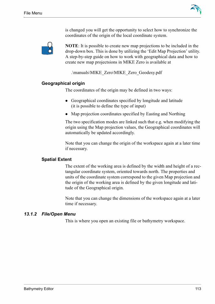
File Menu

is changed you will get the opportunity to select how to synchronize the coordinates of the origin of the local coordinate system.

NOTE: It is possible to create new map projections to be included in the drop-down box. This is done by utilizing the ‘Edit Map Projection’ utility. A step-by-step guide on how to work with geographical data and how to create new map projectsions in MIKE Zero is available at

.\manuals\MIKE_Zero\MIKE_Zero_Geodesy.pdf

Geographical originThe coordinates of the origin may be defined in two ways:

Geographical coordinates specified by longitude and latitude(it is possible to define the type of input)

Map projection coordinates specified by Easting and Northing

The two specification modes are linked such that e.g. when modifying the origin using the Map projection values, the Geographical coordinates will automatically be updated accordingly.

Note that you can change the origin of the workspace again at a later time if necessary.

Spatial ExtentThe extent of the working area is defined by the width and height of a rec-tangular coordinate system, oriented towards north. The properties and units of the coordinate system correspond to the given Map projection and the origin of the working area is defined by the given longitude and lati-tude of the Geographical origin.

Note that you can change the dimensions of the workspace again at a later time if necessary.

13.1.2 File/Open MenuThis is where you open an existing file or bathymetry workspace.


Dialog Overview

Figure 13.2 Open file menu

13.2 Edit Menu

Clipboard editing operations.

Undo This will undo your last operation

Cut/Copy/Paste Cuts, copies and pastes your selected data through the Windows clipboard

Delete Deletes your selected data. The DELETE keyboard command will also perform the same function.

13.3 View Menu

This is where you add toolbar views, status bar and enable double buffer redraws.

Double Buffer Redraw Double buffer redraw uses a technique where you draw into a bitmap and then copy the bitmap to the display. It gives you a much faster refresh rate of the display, but you sacrifice available system memory.

114 MIKE Zero

Work Area Menu

13.4 Work Area Menu

The Work Area menu provides you access to the main tools for bathyme-try definition, creation, interpolation, editing, overlaying images, turning layers on and off, and presentation.

13.4.1 Set Current Contour LevelThis menu pop-up is where you enter the Current Contour Level (depth). After you set the Current Contour Level value, all manual input data will acquire that depth value until you change the value of the Current Contour Level.

13.4.2 Grid Bathymetry ManagementThis is where grid bathymetries are defined, re-defined, interpolated and exported to other formats. The system will allow you to manage a number of grids originating from a single raw data source.

For more information see 13.5 Grid Bathymetry (p. 120).

Figure 13.3 Grid bathymetry management, main dialog

New New Bathymetry is where you can define a grid bathymetry within the workspace.

Edit Edit Bathymetry is where you can edit the definition of a previously defined grid bathymetry.

Delete This is where you can delete a previously defined grid bathymetry.


Dialog Overview

Export Export Bathymetry is where you can export the grid bathymetry to various formats such as binary data files or ASCII formats or as a depth encoded BITMAP graphic file.

Interpolate Interpolate Bathymetry is where you can define the interpolation method and interpolate the defined grid to a digital grid.

13.4.3 Line Bathymetry ManagementThis is where line bathymetries are defined, re-defined, interpolated and exported to dfs1 files. The system will allow you to manage a number of lines originating from a single raw data source.

For more information see 13.6 Line Bathymetry (p. 126).

Figure 13.4 Line bathymetry management, main dialog

New New Bathymetry is where you can define a line bathymetry within the workspace.

Edit Edit Bathymetry is where you can edit the definition of a previously defined line bathymetry.

Delete This is where you can delete a previously defined line bathymetry.

Export Export Bathymetry is where you can export the generated line bathymetry to a dfs1 file.

116 MIKE Zero

Work Area Menu

Interpolate Interpolate Bathymetry is where you can define search radius for the points used in the interpolation.

Presently it is only possible to project the points directly to the line. Note that a work area using LONG/LAT will produce inaccurate results for this type of bathymetry.

13.4.4 Background ManagementThe Background Management system provides you the utility of bringing external data sources into the Bathymetry Editor program. Your back-ground data can either be imported x,y,z data to be added to the raw data-base, or it can be image files to provide background images much like a GIS system. You can control the visualization attributes of the data in Set-tings.

Figure 13.5 Background management


Dialog Overview

Import

Figure 13.6 Import files into background

Normally you first import data in the background into your work area. Types of data which you can import into the background include digitizer files, MIKE 21 XYZ-files, graphical BITMAP and GIF file formats. Before you can import graphical files into the Bathymetry Editor, you need to rectify the image to a compatible coordinate system defined for your work area. (see MIKE Zero Image Rectifier for details on preparing graphic files for the Bathymetry Editor).

When you import MIKE 21 XYZ files you can specify the source coordi-nate system. When the XYZ-file is selected but before the “Open”-button is pressed or a double click is executed, the source coordinate system can be specified by selecting from the “Convert from”-combo box. Coordi-nates can be imported without conversion, as longitude/latitude or by vari-ous map projections. Note that datum shift will not be considered during this automatic conversion.

A number of background sources can be imported into your work area. If you no longer need a background source, simply highlight the background source you want to delete and then click the DELETE option.

118 MIKE Zero

Work Area Menu

13.4.5 Export raw data to XYZ formatYou can export selected raw data to xyz format using this facility. Two ASCII files will be generated. A land file and a water file.

13.4.6 Resize workspace areaThis is where you can re-define your Workspace Area with a new Spatial Extent and a new Geographical Origin.

13.4.7 SettingsThe settings panel allows you to control the attributes for the 4 main lay-ers; Bathymetry Objects, Line Bathymetry Objects, Raw Data Objects and Background Objects. By turning on or off certain layers you can view and edit these layers either individually or in combination with other layers. You can display each object as either points, lines or labels where you can also define the point size, line size and color given to each layer independ-ently.

Figure 13.7 Settings panel

Bathymetry Objects Bathymetry Objects are those that have been interpolated into a fixed grid. You can control Point, Line and Label attributes.


Dialog Overview

Line Bathymetry Objects Line Bathymetry Objects are those that have been interpolated onto a fixed line. You can control Point, Line and Label attributes.

Raw Data Objects Raw Data Object or Foreground objects are those that are available to be interpolated. You can control raw data objects defined as Points, Contour Points, Contour Lines, Land/Water Points, Land/Water Lines and Labels.

Background Objects Background objects are those you have imported, but are not yet available to be interpolated. You can control background objects defined as Points, Contour Points, Contour Lines, Land/Water Points, Land/Water Lines and Labels. To bring background images and data into the Foreground and produce Raw Data Objects, you should use the ToolBar Functions.

13.4.8 Set FontYou can set the font attributes here from this menu.

13.4.9 Show Background ImagesIf you have imported a graphical image into the Background objects, then you can turn the display of the background on or off here.

13.5 Grid Bathymetry

A grid bathymetry defines a dfs2 file containing bathymetry information.

13.5.1 New BathymetryYou define a digital grid by specifying the Geographical Origin and Orien-tation of the grid (in UTM or Geographic coordinates), and some Overall bathymetry properties that includes the grid resolution and specification of land.

120 MIKE Zero

Grid Bathymetry

Figure 13.8 Define digital grid for bathymetry

Geographical Origin You must specify the position of the origin for your grid bathymetry in map projection or Long/LAT coordinates.


Dialog Overview

The geographical position of the origin of the grid is defined as the centre point in the first grid cell (j,k) = (0,0).

Figure 13.9 Definition of Origo

NOTE: If the map projection is defined as NON-UTM, the origo is defined as the lower left corner of cell (j,k) = (0,0).

OrientationThe orientation of your grid is defined as the angle between true north and the y-axis of the grid measured clockwise (“North to Y orientation”). A mnemonic way of remembering this definition is by thinking of NYC, which normally means New York City, but which for our purpose means "from North to the Y-axis Clockwise", see Figure 13.10.

Figure 13.10 Definition of North to Y orientation

The grid rotation defines the clockwise rotation of the grid from map pro-jection north to model north (y-axis of the grid).

PLEASE NOTE: In general the grid rotation is not equal to the North to Y orientation as the map projection north deviate increasingly from true

122 MIKE Zero

Grid Bathymetry

north the longer away from the center of the map projection domain the model area is placed, see Figure 13.11.

Figure 13.11 Left: Chart north (Nc) and true north (NT) for single UTM zone.Right: Difference between Grid rotation and North to Y orientation.

Overall bathymetry properties

Grid Spacing You must specify the distance between grid points in the x and y direc-tions, in metres.

Grid Dimensions You must specify the number of grid points in the x and y directions.

Land Value You must specify the limiting grid cell value defining land. All values above this will be considered to be land.

Display Border You can choose to display the boundary of your defined grid in the Work Area after interpolation.


Dialog Overview

Display Grid Points You can choose to display the grid points of your defined grid in the Work Area after interpolation.

13.5.2 Edit BathymetryYou can re-define a previously defined digital grid here by changing the origin (in UTM or LONG/LAT coordinates), the orientation of the grid, the x and y grid spacing, the number of grid points in x and y, and the land value.

13.5.3 Export BathymetryYou can use this facility to export your interpolated digital grid to another format such as binary data files or ASCII formats, or to a graphical Depth BITMAP file.

Figure 13.12 Export interpolated digital grid bathymetry to another format

13.5.4 Interpolate BathymetryThis is where you specify how your raw data is interpolated to the fixed grid as has been specified in the bathymetry definition.

124 MIKE Zero

Grid Bathymetry

Figure 13.13 Interpolate raw data to fixed grid

Land Generation (Phase I) There are 2 methods for interpolating the land:

1 Polygon Fill

2 Extensive

If your land boundaries have been entered as polygons, then all areas inside the polygon are assigned the value of +10m which is the usual default land value. If you are using land polygons you would choose the polygon fill method. This is a much faster interpolation scheme than the Extensive method that interpolates all grid points based on nearest raw values. You would choose the extensive method if you do not have land polygons, or if you want to interpolate true topographic elevations.

Box Grouping (Phase II) This option specifies how the raw data points are sorted. Currently the raw data points can only be sorted by grouping them by their cell index.

Gap Filling (Phase III) This is where you choose which interpolation technique will be used for gap filling at grid points where no land exists. You specify a search radius that defines how many grid points the search will extend. There are cur-rently 4 search methods available to you.

1 Bilinear interpolationFour points from the raw data, in the vicinity of the actual point, are found in such a way that there is a point in each quadrant. These points


Dialog Overview

now form a quadrangle (or quadrilateral) that encapsulates the grid point. This quadrangle is now transformed into a normalized square (rectified), and bilinear interpolation is performed.

2 Triangular interpolationThree points from the raw data, in the vicinity of the actual point, are found in such a way, that they form a triangle that encapsulates the grid point. Triangular interpolation is now performed.

3 Inverse distance weighted interpolationFour points from the raw data nearest to the actual point measured in each main direction are selected. The inverse distance from the actual point determines the weight of each point in the interpolation.NOTE: The result may be affected by the orientation of the grid

4 Inverse squared distance weighted interpolationFour points from the raw data nearest to the actual point measured in each main direction are selected. The inverse squared distance from the actual point determines the weight of each point in the interpolation.NOTE: The result may be affected by the orientation of the grid

13.6 Line Bathymetry

A line bathymetry defines a dfs1 file containing bathymetry values or rel-ative coastline position.

13.6.1 New bathymetryYou define a digital line by specifying the Geographical origin and Orien-tation of the line (in map projection or geographic coordinates).

You also define some overall Overall bathymetry properties that includes the type of line and line resolution.

Geographical originYou must specify the position of the origin for your line bathymetry in map projection or Long/LAT coordinates.

The geographical position of the origin is defined by grid point 0.

126 MIKE Zero

Line Bathymetry

Figure 13.14 Definition of Origo for line

OrientationThe orientation of your line is defined as the angle between true north and the direction of the line measured clockwise.

Figure 13.15 Definition of North to Y orientation

PLEASE NOTE: In general the line rotation is not equal to the North to Y orientation as the map projection north deviate increasingly from true north the longer away from the center of the map projection domain the model area is placed, see Figure 13.16.


Dialog Overview

Figure 13.16 Left: Chart north (Nc) and true north (NT) for single UTM zone.Right: Difference between Line rotation and North to Y orientation.

Overall bathymetry properties

Type of 1D bathymetryYou must specify the type of bathymetry. You can choose between

Cross-shore profile(will contain bathymetry values along the line)

Coastline position(will contain distance from raw points to the line)

Grid Spacing You must specify the distance between grid points along the line.

Grid Dimensions You must specify the number of grid points on the line.

Display Line You can choose to display the extension of your defined line in the Work Area.

Display Grid Points You can choose to display the grid points of your defined line in the Work Area.

128 MIKE Zero

Window Menu

13.6.2 Edit bathymetryYou can re-define a previously defined digital line here by changing the origin (in UTM or LONG/LAT coordinates), the orientation of the line, the grid spacing and the number of grid points.

13.6.3 Export bathymetryYou use this facility to export your interpolated digital line to a dfs1 file.

13.6.4 Interpolate bathymetryThis is where you specify how your raw data is interpolated onto the fixed line that as has been specified in the bathymetry definition.

Search radiusYou specify a search radius that defined how near the points have to be to the defined line in order to be included in the interpolation.

Figure 13.17 Interpolate raw data to fixed line

Note: presently it is only possible to apply Linear interpolation.

Linear interpolationThe data on the line is derived by first projecting the raw data points per-pendicular onto the line. The values on the line is then interpolated line-arly and the values extracted in the grid point positions along the line.

13.7 Window Menu

This provides you the standard Windows views, and allows you to switch between different open windows.


Dialog Overview

13.8 ToolBar Functions

The following describes the main editing functions that are available to you from the toolbar.

Zoom Functions

You can Zoom-in, Zoom-out and go to Previous-zoom and Next-zoom. You can recall all available previous and next zooms. If the buttons are grayed-out there are no previous or next zooms available. These functions are also available to you by right-clicking the pointer device.

Grid Function

Switch to turn grid on and off.

Pick Mode

Pick Mode. When you enable pick mode, raw data points (foreground points) can be selected by dragging the mouse over the points of interest while depressing the left-mouse button.

Move Mode

Move Mode. If you depress the left-mouse button while over a point you wish to move, the point can be dragged to a new location.

Import From Background

Import From Background mode. With this mode, you can select the back-ground points you want to be brought to the foreground to become part of

130 MIKE Zero

ToolBar Functions

the digital grid bathymetry. Click the Import From Background toolbar button. Highlight the background points you wish to import (single points or area selection). After the background points have been highlighted you then click on the Import From Background toolbar button again. The background data will be transferred to the foreground and become raw data points.

Add Data Points Mode

Add Data Points Mode. In this mode, you click the mouse on a position in the work area, resulting in a raw data point with a depth equal to the cur-rent contour level.

Add Contours Mode

Add Contours Mode. In this mode, you hold down the left-mouse button and drag the mouse. It will place consecutive points of a contour line in the work area as raw data points with a constant depth equal to the current contour level.

Add Land/Water Polygons Mode

Add Land/Water Polygons Mode. In this mode, you hold down the left-mouse button and drag the mouse. This will place consecutive points of a polygon used to define land/water boundaries. These points will go into the raw data layer. For land the current contour level should be set to a value of +10.

Add Points to Contours or Land/Water or Polygons Mode

Add Points to Contours or Land/Water Polygons Mode. In this mode, you hold down the left-mouse button near the end point of a contour or poly-gon. This will allow you to add more points to the existing contour entity.


Dialog Overview

Select Polygons or Contours Mode

Enables selection of entire polygons or contours. By left clicking when touching just a small part of the polygon/contour the entire polygon/con-tour is selected.

NOTEThe minimum digitization distance between consecutive points when dig-itizing in the Bathymetry Editor is 5 units of whatever local coordinate system the working area has been defined in. When working in longi-tude/latitude type coordinate systems, this is a significant distance and the user will experience it impossible to digitize when working in smaller areas. In such cases, the user should digitize in an alternate coordinate sys-tem using length units. The digitized values may then be exported to a xyz file and subsequently imported into a Bathymetry Editor setup using a lon-gitude/latitude type coordinate system.

132 MIKE Zero

M E S H G E N E R A T O R

133

134 MIKE Zero

14 INTRODUCTIONThe Mesh Generator provides a work environment for creating detailed digital mesh for use in the MIKE Zero flexible mesh (FM) models.

Providing these new generation models with a suitable mesh is essential for obtaining reliable results from the model simulations. MIKE Zero offers the MIKE 21 Flow Model FM, MIKE 3 Flow Model FM and MIKE 21 Spectral Wave Model FM, which all are based on a flexible mesh.

Figure 14.1 Land/Water boundary for a domain covering the Planet Earth

Setting up a mesh includes appropriate selection of the area to be mod-elled, adequate resolution of the bathymetry, flow, wind and wave fields under consideration and definition of codes for open and land boundaries. Furthermore, the resolution in the geographical space must also be selected with respect to stability considerations.

You generate a mesh file with the MIKE Zero Mesh Generator. The mesh file is an ASCII file (.mesh extension) that includes information of the geographical position and water depth at each node point in the mesh. The file also includes information about the node connectivity of the triangular and quadrangular elements. All the specifications for generating the mesh file are saved in a Mesh Definition File (.mdf extension), which can be modified and re-used.

Mesh Generator 135

Introduction

The Mesh Generator includes utilities for importing raw data from various external sources (e.g. XYZ soundings, XYZ contours, MIKE 21 bathymetries, MIKE C-MAP exported data), or to manually create data by using the built-in drawing tools. You can import background images such as maps in the Mesh Generator and use them when editing data or for e.g. enhancing presentation graphics.

14.1 Concepts

Your work with the Mesh Generator revolves around inserting and defin-ing nodes, vertices, arcs and polygons. It is therefore important that you understand the meaning of these concepts, shown in Figure 14.2.

Figure 14.2 Concepts in Mesh Generator

A node defines the start and end point of an arc. A closed arc will only have one node while an open arc will have two nodes.

A vertex is an internal point along an arc.

An arc is a number of line segments composed of zero or more vertices and one or two nodes.

136 MIKE Zero

Boundary Definitions

A polygon is a closed loop composed of one closed arc, or two or more open arcs. A polygon is not explicitly defined by the user - it is auto-matically generated when closing an arc or a set of arcs. A polygon can (but not necessarily) be assigned to be a 'zone', which can be given a name. By defining a zone, the polygon can be included or excluded (e.g. representing an island) from the domain or may be identified as a region where a quadrangular mesh is required. Basically, your work with the Mesh Generator should end up with the definition of one large polygon that defines the domain and a number of smaller polygons defining land areas and quadrangular mesh areas within the domain area.

. Note: The terms domain area and workspace area refer to the areas that are to be modelled with one of the FM models and the area in which you are working within the Mesh Generator, respectively. The domain area is a subset of the workspace area.

Your work with the Mesh Generator comes in three phases:

1 Definition of the model boundaries - closed boundaries (land-water) and open boundaries (see Boundary Definitions). You define the boundaries by importing land-water boundary files or by drawing arcs in the workspace area.

2 When you are satisfied with the model boundary, you generate a depth-independent mesh. You can control the mesh generation by defining a maximum triangle area, maximum skewness of the triangles and a maximum number of generated mesh points. Further you may identify areas defined by ‘zones’ within which the mesh may be constructed as quadrangular or defined by another maximum triangle area.

3 In the last phase you can refine the mesh by scaling the element areas according to the water depth at the element center point (this requires the import of water depth information) or modify the mesh using the Mesh Editing facilities. You can define different polygons within the workspace area and modify the mesh within the areas independently of each other.

14.2 Boundary Definitions

You distinguish between closed and open boundaries through the point attribute parameter. For each node in the grid you shall specify an attribute value. You do this by selecting the node (or nodes), right-clicking and selecting properties. From the Point Properties dialog box you can enter the node attribute value, see Figure 14.3.

Mesh Generator 137

Introduction

Figure 14.3 Defining node attribute value

The numeric value of the attribute field (the field labeled ‘a’ on the dialog) is important. The value is used to distinguish between the different open boundaries in the mesh. Later when you apply the generated mesh in a model setup, you will be asked to associate each open boundary defined in the mesh with a boundary condition. You shall use a value of ‘1’ for all closed (i.e. land-water) boundaries in the mesh, whereas all open bounda-ries must be defined with a number > 1.

Note: Per default the Mesh Generator assumes that all boundaries are land boundaries when generating the mesh. I.e. you only have to specify attribute values for open boundaries.

Hint: you can select an arc and specify an arc attribute value, which will-then be used as attribute for all points (vertices and nodes) along the arc.

14.3 Context sensitive menu

You gain access to the context sensitive menu by right-clicking the mouse in the graphics area, see Figure 14.4.

In this menu you may define the selection property (node, rectangle or polygon) or change the view.

Figure 14.4 Context sensitive menu

138 MIKE Zero

Introduction

15 GETTING STARTED

15.1 Introduction

This chapter offers a brief introduction to mesh generation with the Mesh Generator. The following example guides you through the setup of a mesh for Funningsfjord - a fjord on the Faeroe Islands.

The example consists of the following steps:

Step 1 - Create a New Mesh Generator WorkspaceStep 2 - Import Model BoundariesStep 3 - Editing the Land BoundaryStep 4 - Specification of DomainStep 5 - Specification of BoundariesStep 6 - Mesh GenerationStep 7 - Smooth the Land BoundaryStep 8 - Smoothing the MeshStep 9 - Interpolation of a Bathymetry to the MeshStep 10 - Using Polygons to Control the Node DensityStep 11 - Using Polygons to Define Mesh Resolution TypeStep 12 - Analyse the mesh

NOTE: A comprehensive Step-by-step training guide for the Mesh Gener-ator is provided with the MIKE Zero installation. The training guide (PDF-format) can be found in installation folder at

.\MIKE Zero\Manuals\MIKE_ZERO\Mesh_Generator_Step_By_Step.pdf

15.2 Data Location

The data files used in the example are located in the default MIKE Zero installation folder at

.\MIKE Zero\Examples\MIKE_Zero\MeshEdit

15.3 Step 1 - Create a New Mesh Generator Workspace

From the MIKE Zero File menu select New->File->Mesh Generator. You must specify the projection of your coming mesh, before the Mesh Gener-ator can create a workspace for you to work with.

Mesh Generator 139

Getting Started

The Mesh Generator starts by prompting you for a map projection as shown in Figure 15.1.

Figure 15.1 Workspace projection

Please specify the projection as WGS_1984_UTM_Zone_30N.

The Mesh Generator then creates a workspace and you are ready to initiate with the mesh creation process.

15.4 Step 2 - Import Model Boundaries

Model boundaries consist of two types:

The boundary(ies) between land and water.These boundaries are named land boundaries.

The boundary(ies) where you expose boundary conditions (water level, flux variations or wave spectra) when preparing a model simulation. These boundaries are named open boundaries.

The easiest way to define model boundaries is by using the MIKE C-MAP tool. MIKE C-MAP is a global database with water depth and land-water boundaries. You can zoom to a specific area in MIKE C-MAP and export land-water boundaries and water depth values for use with the Mesh Gen-erator.

Two data files are supplied with the example:

land.xyz defining land boundaries

water.xyz giving water depth at a number of points within the area

The area from where data has been extracted is shown in Figure 15.2.

140 MIKE Zero

Step 2 - Import Model Boundaries

Figure 15.2 Funning Fjord

From the Data menu please select the Import Boundary… menu item and browse to the land.xyz file. After having selected the land.xyz file, you will be presented with a Boundary Attribute dialog as shown in Figure 15.3.

Figure 15.3 Boundary Properties

In this menu you shall specify the layout of the land.xyz file, the projec-tion of the data and how to interpret the data. The Reference Guide pro-vides details on import formats.

Mesh Generator 141

Getting Started

Please specify the values as shown in Figure 15.3.

Note: The projection here is specified as LONG/LAT meaning that the data in the land.xyz file are in longitude and latitude. The Mesh Generator will convert the longitudes and latitudes to easting and northing coordi-nates in the UTM-30 projection.

The Mesh Generator reads the data file and updates the workspace as shown in Figure 15.4.

Figure 15.4 Imported Boundary Data

It is only the area in fjord itself that shall be modelled, i.e. the Mesh Gen-erator shall only generate a mesh within the fjord. From Figure 15.4 it can be seen that the area to be modelled consists of:

One open model boundary at the north-east corner of the model area

Land boundaries along the west and east part of the fjord

The next step involves cleaning the workspace for unnecessary land-water boundary points.

142 MIKE Zero

Step 3 - Editing the Land Boundary

15.5 Step 3 - Editing the Land Boundary

During this step you shall remove all points that are located outside the model area as depicted in Figure 15.4.

Please start by deleting the points and arc segments from the left part of the workspace. You select the Delete points button (the eraser) in the tool-bar and click on the points and arcs in the left part of the window. This is illustrated below in Figure 15.5.

Figure 15.5 Delete points and arc segments

You can delete multiple objects quickly by outlining a rectangle or a poly-gon. Try to remove the points and arcs in the left side of the workspace as follows: Select the Delete points button in the editing toolbar, press the left button and drag the mouse over the points, see Figure 15.6. When the button is released all points and arcs inside the rectangle are removed.

Mesh Generator 143

Getting Started

Figure 15.6 Delete points and arcs in outlined rectangle

You may delete entire arcs and related points by first selecting the arc by the arc selection tool, and then pressing the Delete key on the keyboard, see Figure 15.7.

Figure 15.7 Delete selected arcs

144 MIKE Zero

Step 3 - Editing the Land Boundary

It is also possible to delete multiple points and arc segments by enclosing them within a polygon and pressing the Delete key on the keyboard.

Please try the following:

1 From the editing toolbar select the Select points function

2 Right click the mouse to display the workspace context menu and select Inside Polygon

3 Add corners to the polygon by left clicking the mouse. Make a polygon around the line of land in the upper left corner of the window

4 Finish the polygon by double left clicking the mouse

5 Press the Delete key on the keyboard and all points within the polygon are deleted

This course of action is illustrated in Figure 15.8.

Figure 15.8 Polygon selection

You should end up with a land boundary as shown in Figure 15.9.

Mesh Generator 145

Getting Started

Figure 15.9 Final land boundary

Please note that the land boundary as shown in Figure 15.8 consists of one open arc (with two nodes). This has been achieved by converting all land nodes to vertices. During this process make sure that possible holes in the land boundary are closed - depending on how you have cleaned the work-space you might have to close holes.

15.6 Step 4 - Specification of Domain

You have to defined the domain area as a polygon. This allows the area to be triangulated, as only closed areas (polygons) can be triangulated

A new arc closing the fjord must be drawn at the upper right corner of the model area. This new open boundary arc uses the same nodes as the land boundary arc. To draw this arc, select the Draw Arc tool and click on the 2 nodes at the entrance of the fjord, see Figure 15.10.

146 MIKE Zero

Step 5 - Specification of Boundaries

Figure 15.10 Draw boundary arc by connecting two existing nodes

15.7 Step 5 - Specification of Boundaries

It is important to distinguish between land and open boundaries. As explained in Step 4 - Specification of Domain, the domain area as depicted in Figure 15.10 has both a land and an open boundary. By default the Mesh Generator assumes that all boundaries are of type land. You will have to specify that the boundary at the upper right corner is an open boundary.

Please select the Select Arc function in the editing toolbar and select the Open Boundary Arc. Right click and select properties. In the dialog box please specify the arc attribute as 2, see Figure 15.11. This is an indication to the model simulation program that this is an open boundary.

Mesh Generator 147

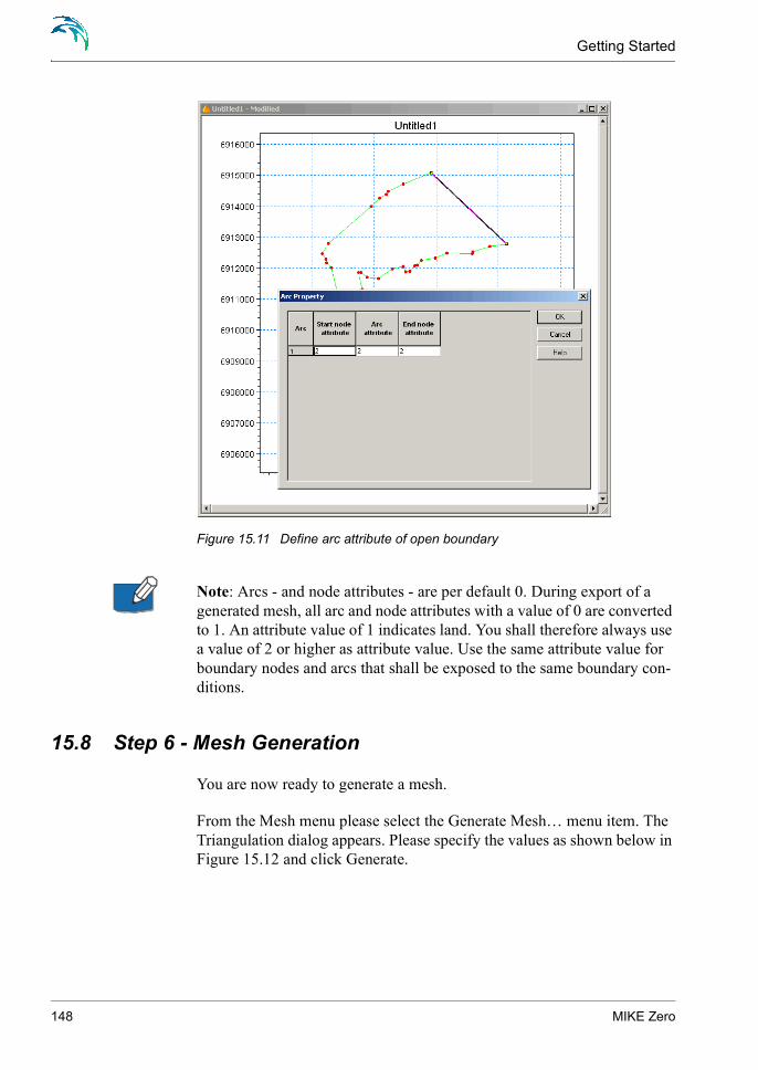
Getting Started

Figure 15.11 Define arc attribute of open boundary

Note: Arcs - and node attributes - are per default 0. During export of a generated mesh, all arc and node attributes with a value of 0 are converted to 1. An attribute value of 1 indicates land. You shall therefore always use a value of 2 or higher as attribute value. Use the same attribute value for boundary nodes and arcs that shall be exposed to the same boundary con-ditions.

15.8 Step 6 - Mesh Generation

You are now ready to generate a mesh.

From the Mesh menu please select the Generate Mesh… menu item. The Triangulation dialog appears. Please specify the values as shown below in Figure 15.12 and click Generate.

148 MIKE Zero

Step 6 - Mesh Generation

Figure 15.12 Mesh generation

The Mesh Generator now calculates and draws a mesh as shown in Figure 15.13.

Note: The Boundary Definition toolbar becomes disabled when the mesh has been generated and the Mesh Editing toolbar is enabled instead. If the mesh is deleted from the workspace the process is reversed. Pls. see Tool-bar Functions (p. 199).

Figure 15.13 Generated mesh

Mesh Generator 149

Getting Started

15.9 Step 7 - Smooth the Land Boundary

If the generated triangles appear unsatisfactorily - e.g. being too small or too large close to land - you have different options. One option is to smooth the land boundary.

Please delete the mesh by selecting the Mesh menu and then the Delete Mesh menu item. Thereafter select the Land Boundary Arc and right-click the mouse and select Redistribute vertices. You are presented with a dia-log box as shown in Figure 15.14.

Figure 15.14 Redistribute vertices

Please specify the values as shown in Figure 15.14 and press OK.

Note: You should always try with a preview before accepting the redistri-bution. With very complex geometries, the redistribution can fail with an unusable land boundary as result.

The new land boundary should be as shown in Figure 15.15. As you can see, the land boundary appears much smoother.

150 MIKE Zero

Step 7 - Smooth the Land Boundary

Figure 15.15 Land boundary after redistribution

A triangulation with the new land boundary results in a mesh generation as depicted in Figure 15.16.

Note: The points are placed much more regular along the boundary line than what was the case with the “raw” boundary line as shown in Figure 15.13.

Mesh Generator 151

Getting Started

Figure 15.16 Triangulation after redistribution of the land boundary

15.10 Step 8 - Smoothing the Mesh

Often you will have to ensure that the variation with respect to area and skewness between neighbouring triangles are kept as small as possible, i.e. creating smooth transitions between different areas in the mesh.

Please select the Smooth mesh… menu item in the Mesh menu and spec-ify 10 as the number of iterations.

In Figure 15.17 you can see the effect of smoothing the mesh.

152 MIKE Zero

Step 9 - Interpolation of a Bathymetry to the Mesh

Figure 15.17 Effect of smoothing

15.11 Step 9 - Interpolation of a Bathymetry to the Mesh

You can refine a mesh in order to correlate the areas of the generated trian-gles to the water depth. Typically you will want to have smaller triangles in shallower areas than in deeper areas.

Please do the following:

1 Delete the mesh

2 Insert a Polygon marker in the fjord by using the Insert Polygon tool in the Boundary Definition toolbar. Select the marker using the Select Polygon tool, right click and select Properties. Use the tick box to ensure that the zone is included in the Triangulation

3 Generate a mesh - in the Mesh menu select the Triangulate… menu item

Before you can interpolate the Z-values at the mesh nodes, you must import scatter data to interpolate from. You add scatter data from the Man-age Scatter Data… menu item in the Data menu.

Please select the water.xyz file and specify LONG/LAT as projection. After importing the data your display should look as shown in Figure 15.18.

Mesh Generator 153

Getting Started

Figure 15.18 Scatter data view

You can now interpolate the imported scatter data to the mesh nodes. Select the Interpolate… menu item in the Mesh menu. Accept the default values and select Interpolate. After the interpolation has finished, click the Close button and the depth interpolated mesh is displayed as a contour plot. See Figure 15.19 for the result.

Note: It is possible to modify the applied color palette for scatter data and contours individually by selecting menu items in the Data menu and Mesh menu, respectively.

154 MIKE Zero

Step 9 - Interpolation of a Bathymetry to the Mesh

Figure 15.19 Contoured map

You can now refine the mesh in order to take the water depth into consid-eration. In the Mesh menu select the Refine mesh… menu item, choose the Depth/gradient option, accept the default values and click the Refine button. A subset of the mesh before and after refinement mesh is shown in Figure 15.20.

Figure 15.20 Detail of mesh before (left) and after (right) refinement

Mesh Generator 155

Getting Started

You should be able to notice that the areas of the triangles are smaller close to land than out in the middle of the fjord.

15.12 Step 10 - Using Polygons to Control the Node Density

Frequently you will need to have a finer resolution in some parts of your model area than in other parts. You can to a certain degree achieve this by refining the mesh relative to the water depth as shown in Step 9 - Interpo-lation of a Bathymetry to the Mesh.

Another way to achieve this is by dividing the model area in different zones - or polygon areas - and defines different maximum element areas for each zone. This method gives you more control of the mesh generation than refining a mesh relative to the water depth.

In the present example you would probably like to have the inner part of the fjord resolved with smaller elements than the outer part.

Please delete the mesh by selecting the Mesh menu and the Delete Mesh. Thereafter you should divide the model area into two zones - an inner and an outer zone. You do this by converting two vertices half-way up the fjord - one at each side of the fjord - to nodes by right-clicking the vertex and select Vertices to Nodes. You can then draw an arc between the two nodes and thus divide the model area into two zones. This is illustrated in Figure 15.21.

Figure 15.21 Dividing an area into zones

156 MIKE Zero

Step 10 - Using Polygons to Control the Node Density

Note: In Figure 15.21 a number of vertices have been placed between the two nodes. The mesh generation algorithm will use these vertices when generating the mesh. In this way, You can control the layout of the meshes close to the borderline between the two zones.

You place a polygon marker in the two zones by clicking the Insert Poly-gon button in the toolbar and then click first in the outer and then in the inner zone. This is shown below in Figure 15.22.

Figure 15.22 Placing polygon markers

You now have to select the zones and define the maximum element area. Please, click the Select Polygon button in the toolbar, select the inner pol-ygon marker and right-click and select properties. You will be presented with a dialog box as shown in Figure 15.23.

Mesh Generator 157

Getting Started

Figure 15.23 Polygon Properties

Make sure that the Apply Triangular mesh is selected and then specify that the triangulation algorithm shall use a local maximum element size of 5000. Do the same for the outer area and specify 40000 as local maximum element size.

You are now ready to make the mesh. In the Mesh menu, select the Gener-ate Mesh… menu item. The result is shown in Figure 15.24.

158 MIKE Zero

Step 11 - Using Polygons to Define Mesh Resolution Type

Figure 15.24 Triangulation using two zones with different maximum element areas

From Figure 15.24 it is clearly seen that the mesh elements now are smaller in the inner part of the fjord than in the outer part.

Note: It is also possible to use the Mesh Editing feature ‘Re-triangulate selected region’ to modify the mesh resolution in a local area after the mesh has been generated.

15.13 Step 11 - Using Polygons to Define Mesh Resolution Type

In a river the flow direction will often be uniform whereas the flow direc-tion in a sea will be more complex. In areas of uniform directional flow it can often be an advantage to model the flow pattern in a quadrangular mesh. Now try to define the inner part of the fjord by a quadrangular mesh while the remaining part is maintained as a triangular mesh. This requires that the inner part of the fjord is defined by at least 4 arcs and that two of the arcs are only defined by the nodes.

Please do the following:

1 Delete the mesh

2 Convert two vertices in the inner end of the fjord to nodes as shown in Figure 15.25

Mesh Generator 159

Getting Started

3 Convert two vertices at the banks of the fjord to nodes and define a new arc as shown in Figure 15.25

4 Define a new polygon marker in the new inner polygon. Select the pol-ygon marker (this will highlight the polygon and show the arc attribute values)

5 Right click to select Properties. Use the tick box to define the polygon as a quadrangular mesh and specify the options shown in Figure 15.26

6 Generate a mesh - in the Mesh menu select the Triangulate… menu item

This will result in the mesh shown in Figure 15.27.

Figure 15.25 Polygon properties for quadrangular mesh

160 MIKE Zero

Step 11 - Using Polygons to Define Mesh Resolution Type

Figure 15.26 Quadrangular polygon options

Figure 15.27 Resulting mesh in inner fjord using quadrangular elements

Mesh Generator 161

Getting Started

15.14 Step 12 - Analyse the mesh

To ensure that the mesh is optimal for use in the numerical model, the mesh is analysed using the Mesh Analysis option.

First interpolate the scatter data into the node points as shown in section 15.11 while using the triangulated mesh from section 15.12. This creates the bathymetry information that ensure that all options in the Mesh Analy-sis dialog is available.

Select Mesh in the Toolbar, Mesh Editing and then Analyse Mesh. This will give the Analyse Mesh dialog shown in Figure 15.28.

Figure 15.28 Analysing mesh options

The two first options in the Analyse Mesh dialog calculates the time step constraints for each mesh element based on the CFL stability criteria. The latter two options analyse the mesh sololy defined on the mesh element geometry.

162 MIKE Zero

Step 12 - Analyse the mesh

Selecting the zoom button for the smallest time step at the top of the table will cause the display to mark the grid cell and zoom into the local area, see Figure 15.29.

Note: Choosing some of the other analysis options will reveal that the CFL criteria causes the most severe time restriction.

Figure 15.29 Marked grid cell for smallest restrictive time step when calculation is based on the water level.

By using the information from the analysis it is possible to optimize the mesh layout by modifying the mesh resolution locally around the critical mesh elements.

You can now try to optimize the mesh by adding or deleting node points using the Mesh Editing toolbar. Note that each edition may change the result of the analysis.

Mesh Generator 163

Getting Started

164 MIKE Zero

File Menu

16 REFERENCE GUIDEThe following describes the main functions that are available to you from the menubar.

16.1 File Menu

The Mesh Generator provides you with a work environment for creating, editing and presenting detailed digital flexible meshes.

File/New MenuYou use the New menu item in the File menu to create a new mesh docu-ment, i.e. mesh definition file. The only information you initially must specify is the geographical projection of the mesh.

File/Open MenuYou use the Open menu item in the File menu to open an existing mesh document file. All mesh documents have a .mdf as file extension.

16.2 Edit Menu

The edit menu provides options for undoing and redoing previous made changes to the mesh document, for selecting and deleting points and for setting different global Mesh Generator options. Global options are options that cover all editing sessions with the Mesh Generator.

16.2.1 UndoYou use the Undo menu item to undo the last change made to the mesh document. All changes made during an edit session are recorded and can be undone. However, you can define a limit for the number of changes to record from the Options menu item (p. 166).

Note: You can use the keyboard shortcut Ctrl-Z to activate the undo func-tion.

16.2.2 RedoYou use the Redo menu item to redo an undo action. If you have undone too many changes you can come back to a previous state by using the redo function.

Mesh Generator 165

Reference Guide

Note: The redo stack is cleared the first time you make direct changes to a mesh definition, e.g. inserting new nodes.You can use the keyboard shortcut Ctrl-Y to activate the redo function.

16.2.3 DeleteYou use the Delete menu item to delete all selected features, e.g. nodes or arcs.

Note: You can use the keyboard shortcut Delete to activate the delete function

16.2.4 OptionsYou use the Options… menu item to set different Mesh Generator global options, i.e. options that take effect in all Mesh Generator editing sessions.

The undo level specifies how many changes the Mesh Generator should record and make available for undoing. If you are working with a very large setup that requires a lot of memory, you could lower the level and in this way reduce the memory needed for holding the undo buffers.

16.3 View Menu

The View menu provides functionality for overlaying the workspace area with geographical information, for zooming in the data, for adding toolbar views and status bar.

16.3.1 Coordinate OverlaysThis menu item makes it possible to overlay the workspace area with a geographical net showing the latitudes and longitudes and a North arrow.

16.3.2 Zoom facilitiesThe Zoom In menu item gives access to a rubber band you can use to select a sub-area to work with. You use the rubber band to define the sub-area. With the band present; you outline the area by pressing the left mouse button and dragging the band. When you release the button, the workspace area will zoom to the specified area.

The Zoom out menu item resets the zoom level to the full workspace area.

The Zoom to Extent of Data menu item sets the zoom level such that all data points are shown in the workspace area.

166 MIKE Zero

View Menu

16.3.3 Go ToThe Go To menu item shows a dialog you can use to navigate in the work-space.

Figure 16.1 The Go to dialog

You can go to:

A specific coordinate

A specific node in a generated mesh

A specific element in a generated mesh

The largest or smallest element in a generated mesh

The smallest angle element in a generated mesh

The deepest or highest located node in a generated mesh

The most shallow located node in a generated mesh

The dialog also allows you to zoom in on the specified point. Setting the zoom level to a value higher than 100 implies zooming in on a point, and values less that 100 correspond to zooming out.

16.3.4 Drawing options

Fixed Aspect RatioWith the Fixed Aspect Ratio menu item enabled, the workspace area will be drawn using the same scale in both the X- and Y-directions. If you clear the Fixed Aspect Ratio menu item, the workspace area will fill the entire editor window.

Mesh Generator 167

Reference Guide

Double BufferDouble buffer redraw is a technique where you draw into a bitmap and then copy the bitmap to the display. It gives you a much faster refresh rate of the display, but at the cost of reduced available system memory.

16.3.5 Export GraphicsWith the Export Graphics menu item you can copy the workspace area as an image to the clipboard or directly save it in a file as either a bitmap or as a Windows metafile.

This is mainly to be used when preparing presentations or for importing illustrations in reports.

16.3.6 ToolbarThe Toolbar menu item gives access to a toolbar selection dialog.

Note: You cannot deselect the Mesh Generator specific toolbars

16.3.7 Status BarThe Status bar menu item toggles between showing and hiding the MIKE Zero status bar.

16.4 Data Menu

The Data menu provides functionality for importing, exporting and con-verting data.

Note: Some of these menu items are only accessible when the relevant object has been selected.

16.4.1 Import BoundaryThe Import Boundary menu lets you import an XYZ file defining the land-water boundary. After having selected the file with the boundary informa-tion, you have to specify additional information for the editor to correctly interpret the XYZ data.

168 MIKE Zero

Data Menu

Figure 16.2 Import boundary dialog

You need to specify:

1 The layout of the XYZ dataThe data in the file must be formatted as ASCII text in three or four columns with the two first columns giving the X-and Y-coordinates of the points. The remaining one or two columns shall include connectiv-ity information and - optionally - a Z-coordinate defining the water depth at the point. The connectivity column is used to define arcs. All points along an arc - except the last point - shall have a connectivity value of 1 and the last point shall have a connectivity value of 0.

2 The projection of the dataIf the data has a different projection than the workspace area, the data values will be converted to the projection used with the workspace area.NOTE: The automatic conversion does not consider Datum Shift. If required then convert the xyz data using the Datum Convert Utility before adding the data to the setup.

3 How to convert the point values to arcsYou can choose to connect all points to one arc, i.e. omitting the con-nectivity column in the data, or to use the connectivity information and draw multiple arcs. Finally, you can specify a minimum length of arcs (measured in number of points). The latter can for example be used to exclude small islands from the mesh.

Mesh Generator 169

Reference Guide

By selecting the Data Info button you can view the statistics of the XYZ file and the minimum and maximum values of the columns.

Note: When importing boundary data, the Mesh Generator assumes that all closed arcs with a horizontal and vertical extent less than 20 per cent of the full data range represents islands. Such islands will not be included in the triangulation. You can - if needed - later change the status of such automatically detected islands.

Note: In case a vertice point during the import process is recognized to be defined more than once (double-defined), the point is skipped.

16.4.2 Export BoundaryThe Export Boundary menu gives you the option of exporting selected point and/or arcs to an XYZ file. This can be used to e.g. import the data in other models or if you want to manipulate the arcs with another pro-gram like e.g. Microsoft Excel.

16.4.3 CleanWhen importing boundary data you might come in a situation where either some points are placed very close to each other or points are defined more than once (double-defined). The triangulation algorithm cannot triangulate areas with double-points and generates strange meshes with points located very near each other.

With the Clean menu you have the possibility of removing nodes located near each other. You specify a minimum distance between nodes. All nodes with a distance less than the specified threshold value will be removed.

Note: The algorithm can only remove nodes - and not vertices - located near each other. In case your data contains two or more vertices - or a node and a vertex - placed near each other, you will have to manually resolve the problem. Zoom to the point and move or remove points in order to solve the problem. The mesh algorithm will - in case of double points - abort the mesh calculation and report the location of the double points.

16.4.4 Convert Nodes to VerticesWith this menu item you can convert selected nodes to vertices.

Note: Changing a node to a vertex results in merging two arcs into one arc. You cannot convert a node representing a single arc to a vertex.

170 MIKE Zero

Data Menu

16.4.5 Convert Vertices to NodesWith this menu item you can convert selected vertices to nodes.

Note: Changing a vertex to a node results in splitting a single arc into two smaller arcs.

16.4.6 Redistribute VerticesThis menu item provides you with a dialog you can use to redistribute the vertices along selected arcs, e.g. ensuring that all vertices are place with at constant distance apart.

Figure 16.3 Arc Redistribution dialog

You can redistribute the vertices along the selected arc(s) in three different ways:

You can specify the number of vertices along the arc(s)

You can specify the distance between the vertices along the arc(s)

You can divide each segment along the arc(s) in a specified number of segments

The selected arcs are curve-fitted following a spline curve. You can spec-ify the spline factor. A smaller spline factor leads to a smoother curve, but at the cost of moving points.

Note: This menu item is only accessible after you graphically have selected one or more arcs.

Mesh Generator 171

Reference Guide

16.4.7 Manage Scatter Data The Manage Scatter Data menu gives you a dialog from where you can manage your scatter data. You can add, remove or reduce scatter data sets as well as convert scatter data points to nodes or arcs.

It is also possible to modify individual scatter data points using the Scatter Data Toolbar (p. 210).

NOTE: Reducing scatter data sets using the Reduce Scatter Data Set but-ton saves the edited data in a new file. Modifying individual scatter data points using the Scatter Data Toolbar will modify the original scatter data set.

Scatter data is typically used to interpolate bathymetry values to the mesh elements. The range of the various data sources may be viewed at the bot-tom of the dialog for all files or for a selected file. It is possible to zoom to the extent of the range of all scatter data or a selected file.

Furthermore you can choose which data files to display in the graphics.

Figure 16.4 The Manage Scatter Data dialog

Add scatter dataYou can use the following type of files as scatter data:

172 MIKE Zero

Data Menu

XYZ files, ASCII files organised in three columns – X,Y coordinates and the bathymetry value (Z)

DFS2 files, DHI 2D data files containing bathymetries.NOTE: only values below the specified land value are used

DFSU files, DHI flexible mesh filesNOTE: the values are obtained from the static item bathymetry value

Mesh files, files exported from the Mesh Generator with a mesh defini-tion and bathymetry value

NOTE: When you select a xyz file you have to specify the map projection for the data values. In case this map projection is different from the Work-space Projection the coordinate values will be converted automatically however the conversion will not consider Datum Shift. If required then convert the xyz data using the Datum Convert Utility before adding the data to the setup.

From this menu item you also get the opportunity to Convert scatter data to nodes and arcs.

It is possible to prioritize the data in the interpolation process by applying different weights to the data sources (see Prioritize Scatter Data (p. 175)).

Convert scatter dataWith the Convert Scatter Data dialog you can convert imported scatter data to arcs or nodes.

Figure 16.5 Convert scatter data dialog

If you convert scatter data to arcs or nodes you should normally also remove the scatter data file from the list of inserted scatter data file.

Mesh Generator 173

Reference Guide

Note: The action takes effect when you click the OK button and cannot be reversed.

Reduce Scatter Data SetThe Reduce Scatter Data Set menu item displays a dialog that allows you to reduce the number of scatter data points. This can be useful in order to reduce the time it takes to interpolate a bathymetry to a generated mesh.

If the scatter data you have imported has a much finer resolution than the area of mesh element, it is often advantageous to reduce the amount of scatter data.

When reducing the data you first specify in the Manage Scatter Data dia-log if you want to reduce all the scatter data or only the data from a spe-cific file.

Figure 16.6 Scatter data reduction dialog

The Mesh Generator offers three different algorithms for reducing the amount of scatter data:

You can reduce the number of scatter points by defining a maximum number of scatter points per mesh element.

This algorithm scans all scatter points and associates them to the mesh elements. You can specify a maximum number of points per element to retain. You also specify a threshold value for the number of points to retain per pseudo-element outside the convex hull – the outer domain

174 MIKE Zero

Data Menu

of the mesh area. The pseudo-element is taken as an element with an area corresponding to the largest true element.

You can reduce the number of scatter data based by defining a maxi-mum number of points per square unit

This algorithm divides the area in a number of equally sized squares and retains only the first number of specified points per square.

You can reduce the number of scatter data based on the proximity of scatter points.

This algorithm scans all scatter point and detects and removes all points located within the specified distance from the actual point.

Note: When you reduce a scatter data set you have to save the reduced scatter data set to a new file. The new file will be written as an XYZ file.

16.4.8 Prioritize Scatter DataThe Prioritize Scatter Data menu item displays a dialog that allows you to apply different weights for specified scatter data sets and define a sequence of prioritization that is used when you Interpolate the mesh bathymetry.

Mesh Generator 175

Reference Guide

Figure 16.7 The Prioritization dialog

To enable the prioritization functionality you must enable the 'Use Prioriti-zation' check box.

You can define one or several weight combinations in the lower part of the dialog. The corresponding Weight IDs can then be selected for global and/or local prioritization.

The local prioritization are defined in the upper part of the dialog. To be able to use prioritization for only a part of the domain, a Prioritization area must be defined beforehand. In case of several local prioritization areas the order entry defines the sequence of the interpolation.

Prioritization areaA prioritization area is a user defined area where a specific prioritization weight combination is to be used. Prioritization areas are different from the polygons used for specifying mesh resolutions and mesh type. To cre-ate areas for local prioritization use the Prioritization Toolbar (p. 213).

176 MIKE Zero

Data Menu

IntroductionThe input topographical data typically originate from various sources. The multiple sources are reflected in the variation in spatial extent, resolution and quality. As an example one may have data in a coarse resolution for a region and additionally some fine resolution LIDAR for a subarea. For the subarea one would typically solely use the LIDAR data for constructing the bathymetry whereas for the remaining area the coarser regional wide data would be used. Thus the user would preferably assign some rules to the interpolation of the scatter data.

The interpolation prioritization functionality in the mesh editor enables the user to grade the quality of the scatter data globally for the whole model domain as well as locally for subareas of the model domain. The accuracy associated with the various sources may further vary signifi-cantly. This in turn may result in fine scale data being impacted by less accurate data giving rise to synthetic smoothing in the interpolation. To reduce such effects the prioritization of source data may be used. The pri-oritization is carried out by applying weights to the individual data sets. These weights may be assigned globally and locally.

How to use the prioritization functionalityIn the step-by-step example four data sets are used for interpolating the bathymetry values in a generated mesh:

1 Regional lines distributed across the whole domain

2 Local lines in a smaller area

3 Measurements from distinct sub area in front of the harbour

4 Dummy settings for the harbour area

Pls. see the outline of the applied scatter data sets in the figure below.

Mesh Generator 177

Reference Guide

Step 1: Import dataThe data can be loaded into the Mesh Generator using the menu item: Manage Scatter Data. The various data sources are added one by one by clicking the 'Add…' button and selecting the data file. Finally click the 'Apply' button to update the overview.

Once the data files have been selected the window will look similar to the one in Figure 16.4. Note that at the bottom of this window the range of the various data sources may be viewed. Furthermore the zoom button can zoom to the extent defined by a selected data set as shown below.

Step 2: Create prioritization incidentsThe next step is to assign prioritization weights to the data sources. This will be done locally as well as globally. The prioritization will be utilized such that for the area in front of the harbour only the survey data will be applied and in the area covered by local lines the regional lines and local lines will be prioritized by 10% and 90%, respectively. Thus a set prioriti-zation weights are needed for each of the data sets.

178 MIKE Zero

Data Menu

To define the weights access the prioritization dialog through the menu item Prioritize Scatter Data. In the dialog that appears the lower part of the window defines the weight combinations. To activate these you must ena-ble the 'Use Prioritization' check box. Subsequently one can add any number of weight combinations.

In the example shown in Figure 16.7 two weight combinations have been defined: one which only takes the survey data into account and one which uses a combination of Regional lines and Survey lines. Note that the weights must be non-negative values and cannot all be zero.

Step 3: Define prioritization areasTo apply local weights one needs to define areas for which the local weights are to be applied. This is done through the Prioritization Toolbar (p. 213) used for creating and editing prioritization polygons.

Using these tools one can define, move, add, delete and select nodes of a prioritization area. The user is prompted to supply a name for the defined area to be used in the Local prioritization dialog later. Once the area has been defined the view will look similar to the one below.

The SurveyArea area encompasses data from the WeightID Survey and the LocalLinesArea data from WeightID Vicinity.

Mesh Generator 179

Reference Guide

Step 4: Apply prioritization incidents to areasThe next step is to assign the weight combination to the individual prioriti-zation area. This is done through the Prioritize Scatter Data menu. Once the prioritization areas have been defined the upper part of the dialog will be populated with the area names. The only remaining step is to assign the appropriate weight combination ID to the individual prioritization areas. The menu will look similar to Figure 16.7 once the weight combinations have been assigned.

Note that outside the two defined areas (global prioritization) no prioriti-zation is applied which means that all data sources are pooled into one data set which is then used to interpolate the data onto the mesh.

Step 5: Generate mesh and interpolate bathymetryThe next step is to generate the mesh and carry out the interpolation. A comparison of the resulting mesh with and witout prioritization of the scatter data is displayed in Figure 16.8.

180 MIKE Zero

Data Menu

Figure 16.8 Resulting mesh bathymetryUpper: with prioritization of scatter dataLower: without priotization of scatter data

16.4.9 Scatter Data Visualisation

View Scatter DataThis menu item toggles visualization of scatter data. Drawing large amount of scatter data can be time consuming.Toggling scatter data visu-alization off can improve the responsiveness of the Mesh Generator.

You can define which scatter data sources to display from the Manage Scatter Data dialog (see p. 172).

Note: The menu item is only active if scatter data have been imported.

Mesh Generator 181

Reference Guide

Scatter Data Point SizeThis menu items toggles the size of the scatter data points to be shown in the display. You have the option to choose between 10 sizes, see Figure 16.9. The point size is not affected by the zoom level.

Figure 16.9 Scatter data point size: 1 to 10.

Scatter Data PaletteYou may define your own attribute palette for the scatter data point attributes.

View Scatter Data LegendThis menu item toggles between showing and hiding the colour legend that visualizes the colour ramp used when drawing scatter data points.

Note: The menu item is only active if scatter data have been imported.

16.5 Mesh Menu

The Mesh menu provides functionality for importing, generating and exporting a mesh.

16.5.1 Load meshYou use the Load Mesh menu item to import an existing mesh.

This mesh can be utilized as a starting point for modifying the mesh using the Mesh Editing Toolbar (p. 214).

16.5.2 Generate meshYou use the Generate Mesh... menu item to generate a mesh of the area. There are a certain number of rules to follow in order to secure a success-ful mesh generation:

At least three points are required for starting the generation

182 MIKE Zero

Mesh Menu

Mesh generation is only performed within polygons - a polygon is implicitly made of one or more arcs. In order to generate a mesh for a coastal area, you will therefore have to have one polygon covering the full area to be modelled.

The mesh algorithm cannot handle double-defined points. You will have to remove all double-points before a mesh can be generated. You can either remove double-points through the Clean menu item in the Data menu or by editing the points

Mesh generationThe Generate Mesh ...menu leads to a Mesh Generation dialog box from where you can initiate the mesh generation or specify a number options controlling the mesh generation.

Figure 16.10 Mesh Generation dialog

Generation of the triangular part of the mesh is controlled through three parameters that are specified in the Mesh Generation dialog.

The parameters are:

1 The maximum allowable element area measured in m^2 or deg^2 depending on the projection of the workspace area. The algorithm gen-erally seeks to maximize the areas of the elements

2 The smallest allowable angle between two sides in a triangle. This parameter controls the skewness of the triangles

3 The maximum number of generated nodes

Mesh Generator 183

Reference Guide

After the mesh has been calculated the Generate Mesh ... dialog will report the number of elements and nodes that have been generated both for the triangular and the quadrangular part.

Note: Generation of a quadrangular part of the mesh is controlled through the Polygon properties dialog (see p.204).

16.5.3 Smooth MeshThe Smooth Mesh menu item can be used to smooth the triangular part of a generated mesh. Smoothing a mesh means that the differences with respective to area and angles between neighbouring elements are reduced, i.e. the elements are homogenised.

Figure 16.11 Smoothing dialog

Two options can be included when smoothing the mesh:

Smoothing constrained by mesh criterionPrior to mesh generation some constraints on the element area and the angles may be applied. When smoothing the mesh one may disable these constraints by deselecting the check box.

Leave mesh nodes at arcs untouchedIf this check box is deselected ALL internal nodes may be relocated. Otherwise, if a node originally was part of a defined arc or is a single user defined node, then the node is not allowed to be moved during the smoothing.

Note: The smoothing algorithm only applies to triangular mesh elements. If the mesh after smoothing remains the same the overall mesh is as homogenised as can be.

16.5.4 InterpolateThe Interpolation menu item is used for interpolation of scatter data to the mesh nodes. Typically, the scatter data represents the bathymetry in the area, but it could also be other types of spatial data.

184 MIKE Zero

Mesh Menu

Note: In order to perform an interpolation you have to have imported some scatter data to interpolate from. You import scatter data using the Manage Scatter Data menu item in the Data Menu (p. 168).

Figure 16.12 Interpolation dialog

PrioritizationIf you want to utilize prioritization in the interpolation you have to have defined the prioritization weights beforehand using the Prioritize Scatter Data menu item in the Data Menu (p. 175).

Value from scatter dataIf you have a very dense set of scatter data points, you can dramatically decrease the interpolation time by simply assigning the node value from the closest located scatter point. You do this by clicking the Set value from scatter data check box – you should at the same time set a reasonably max-imum search distance.

Mesh Generator 185

Reference Guide

NOTE: Node points assigned a value in this way will not be included in the overall interpolation. E.g. the presence of break lines will not be con-sidered.

TrianglesYou can select between two different algorithms for performing the inter-polation for the triangular part:

Natural Neighbour interpolation

The Natural Neighbour method - which is particularly effective for dealing with a variety of spatial data themes exhibiting clustered or highly linear distributions - is a geometric estimation technique that uses natural neighbourhood regions generated around each point in the data set. The natural neighbourhood regions are determined by creating a triangulated irregular network from the scatter data points.

With the Natural Neighbour method four additional points can option-ally be used in the interpolation. The position of the four points can be controlled through the Size of bounding window parameter. The points will be placed at the lower left, upper left, lower right and upper right corner of the workspace area, respectively. The parameter specifies the distance from the four points to the data extent area. The water depth value at the four points will be defined as the extrapolation value.

You can specify a node value to be used in situations where the Mesh Generator needs to extrapolate in order to calculate the water depth at a node value.

Linear interpolation

The linear method uses a mesh generated from the scatter points when doing the interpolation. For each point to be interpolated a surrounding triangle is determined and a linear interpolation based on the node val-ues is made.

QuadranglesFor the quadrangular part the interpolation settings are set individually for each of the polygon areas. The areas defined by quadrangles are listed at the bottom of the Interpolation dialog. For each quadrangular mesh area the interpolation method used is listed. Further you may choose to zoom to the area in question by clicking the zoom button. Finally the Edit button grants access to the interpolation settings for the individual quadrangular mesh areas.

186 MIKE Zero

Mesh Menu

Figure 16.13 Interpolation options for areas with quadrangular mesh

Within the quadrangular interpolation options you may choose the same methods available for the triangular part. In addition you can choose the Inverse Distance Weigthed method that requires a strength value in both the flow direction and the transversal flow direction. The latter gives the possibility of applying a greater weight to data in the flow direction com-pared to data lying in the transversal direction.

See also Setting up zones with quadrangular mesh elements (p. 205).

16.5.5 Refine MeshA mesh may be refined using one or both of the following methods

Face bisection

Depth/Gradient

Face bisectionYou can refine a mesh by subdividing the faces of the existing elements. This approach is termed 'Face bisection'. The bisection method is designed to only change the size of the elements in a given mesh without changing the overall quality of the mesh, i.e. the angles of the refined mesh will not become less than the original mesh. The approach is illustrated in Figure 16.14.

Mesh Generator 187

Reference Guide

Figure 16.14 Approach for bisection of elementsUpper: Approach for triangular elementLower: Approach for quadrilateral element

The only parameter that is required is the number of bisections to apply. Once this has been selected the start button can clicked and the progress will visualized through a progress bar.

The number of elements grows by a factor of four per bisection applied. Thus using e.g. 3 bisections will make the number of elements grow by 43=64. In general try to select the number of bisections in the range 1-4. In the present version you cannot create a mesh with more than 500.000 ele-ments via bisection.

NOTE: The bisection method may also be invoked when exporting the generated mesh to either a mesh file or a dfsu file.

Depth/Gradient You can refine a mesh in order to take the water depth into account when generating a mesh. Doing so requires:

That the workspace area has been interpolated with respect to water depth

That at least one zone has been defined. A zone is a polygon that can be marked for inclusion or not in the triangulation. You define a zone by placing a zone marker within a polygon and marking the zone (right click the zone point and select properties) for taking part in triangula-tion or not. You can give the zone a name for easier identification

188 MIKE Zero

Mesh Menu

Note: This feature don’t work if the mesh contains any quadrangular ele-ments.

Note: A polygon is a closed loop composed of one closed arc, or two or more open arcs. A polygon is not explicitly defined by the user. It is auto-matically generated when an arc, or a set of arcs, is closed. A polygon can (but does not have to be) assigned to be a zone.

Figure 16.15 Mesh refinement by depth dialog

The refinement option dialog lets you specify the correlation between ele-ment area and water depth or bed level gradient. You can specify both lin-ear and non-linear by choosing the curve (double-click on the curve and drag the generated knot) dependency.

16.5.6 Analyse MeshYou can analyse the mesh for its applicability in a simulation by evaluat-ing the restricting time step for each mesh element. The minimum time step will define the maximum time step for the entire simulation.

Note: You have to be in Mesh Editing mode in order to analyse a mesh.

By using the editing facitilies in the Mesh Editing Toolbar (p. 214) you have the possibility to modify the mesh in selected regions in order to increase the minimum time step and thus decrease the total simulation time for your model.

Mesh Generator 189

Reference Guide

You may analyse the mesh using different options:

Smallest time step based on the water level

Smallest time step based on the water depth

Smallest area

Smallest angle

The smallest time step, dtmin, for each element is found by the limiting CFL number, the length of the smallest face of the element, le, and the total water depth, Dt, as follows:

(16.1)

The resulting table in the dialog contains the upper most restrictive values and you have the option to zoom into each of the elements in the table.Note that you may control the number of elements in the table.

Figure 16.16 Analyse Mesh dialog

dtmin12--- CFL le 9.8Dt( )⁄⋅ ⋅=

190 MIKE Zero

Mesh Menu

16.5.7 Arc/Mesh editing modesThe mesh editor has two main modes when editing:

Arc editing mode

Mesh editing mode

The Arc editing mode is used for setting up the arcs and single nodes which make up the skeleton for generating the mesh. The Arc editing mode is typically only used initially to get the overall working area defined along with delineation of coast lines or other specific topographi-cal features in the domain.

The Mesh editing mode on the other hand is used when modifying an already generated mesh e.g. merging triangular elements or moving indi-vidual mesh nodes. Keep in mind that if the mesh is subsequently regener-ated all mesh editing will be lost.

To switch between the two modes select the 'Mesh' menu and then choose either 'Arc Editing' or 'Mesh Editing'. When selecting Arc editing a possi-ble mesh will be displayed by a paler shade of color and any Mesh editing tools are inactive. Similarly choosing the mesh editing mode inactivates Arc editing tools and all arcs in the set-up will be visualized by a stronger mesh color, see Mesh Visualisation (p. 192).

Note: You can use the keyboard shortcut Ctrl-M to toggle between the two modes.

16.5.8 Delete MeshThe Delete Mesh menu item deletes a generated mesh.

16.5.9 Export MeshYou use the Export Mesh functionality to export a generated mesh to a file for use in one of the simulation models in the FM-series.

Note: You cannot use the Mesh Generator document file (.mdf-file) with the simulation models. You will have to export the mesh to a .mesh file in order to use it in a model simulation.

Export asTypically, you will export the mesh as a .mesh file - an ASCII-file defin-ing the node positions, the element topology and the depth at the nodes. This information defines the necessary information for the FM-simulation models for setting up the computational grid.

Mesh Generator 191

Reference Guide

You can also select to save the data as a .dfsu file. Such a file cannot be used as a mesh-definition file with the simulation models. However, you can use this possibility to generate e.g. bottom friction and eddy viscosity maps for the simulation models.

Additional refine meshThe Face bisection may also be invoked when exporting the generated mesh to either a mesh file or a dfsu file. In that case the program generates two files:

1 The original mesh in the format (*.dfsu or *.mesh) selected by the user

2 A refined mesh where the refinement algorithm has been applied.

The latter file will be given the name 'filename_refined.*' where the origi-nal mesh is saved in a file named filename.*. The extension being either mesh or dfsu.

Note: The additional refined mesh is only generated if the user checks the 'Create refined mesh'. This feature may be used to carry out simulations with same mesh structure but different resolutions.

ExampleTo make a .dfsu file including e.g. a bottom friction map instead of bathymetry you do the following:

1 Generate the mesh you want to use in a simulation

2 Specify bottom friction values covering the model area as either a XYZ-file or as a .dfs2-file

3 Load the mesh file into the Mesh Generator

4 Add the bottom friction values as scatter data

5 Interpolate the bottom friction values to the mesh

6 Export the Mesh to a .dfsu-file through the Export Mesh menu. You can give a descriptive name to the data you export, e.g. "Bottom Friction.dfsu".

16.5.10 Mesh Visualisation

Draw meshThis menu item toggles between displaying and hiding a generated mesh.

192 MIKE Zero

Options Menu

Mesh ColorThis menu items toggles the main color of the mesh shown in the display. You have the option to choose between black, yellow, red or blue. The shade of the color is determined by the choice of Arc/Mesh editing modes (p. 191).

View Mesh Element NumbersThis menu item toggles between drawing mesh element numbers in each generated mesh element.

View Mesh Node NumbersThis menu item toggles between drawing node numbers at each generated mesh node.

Note: Some menu items are only accessible after a mesh has been gener-ated or loaded.

16.5.11 Contour Visualisation

Contour typeWith this menu you can toggle between showing the interpolated water depth as a box contour map or as a shaded contour map. A box contour map differs from a shaded contour map by colouring a triangle according to the depth of the centre of gravity point of the triangle. A shaded contour map is drawn without relation to the generated mesh.

You also have the option to set the transparency of the contour map.

Contour paletteYou may define your own attribute palette for the contour map.

View Scatter Data LegendThis menu item toggles between showing and hiding the colour legend that visualizes the colour ramp used when drawing the contour map.

Note: The last menu item is only active if a contour map exist.

16.6 Options Menu

This menu lets you set different options with respect to projection, work-space area, various graphics parameters and mesh editing.

Mesh Generator 193

Reference Guide

16.6.1 ProjectionThis menu item gives you the possibility of selecting or changing the pro-jection of the workspace area or data. If data points have already been inserted in the area, they will also be converted to the new projection.

Figure 16.17 Workspace projection dialog

Note: The automatic conversion of coordinates does not consider any datum transformation. If this is required then use the MIKE Zero Datum-Convert utility to convert the data before entering the data into the Mesh Generator.

16.6.2 WorkspaceFrom this menu you can redefine the size of the workspace area.

Note: you have to "Zoom Out" in order to redraw the workspace area to the new extent.

16.6.3 Import Graphic LayersThis menu lets you import image files and use them as background in the workspace area. You have to specify the path of the images. In case the image is georeferenced the positioning and extent of the image in the workspace area is automatically set. Otherwise you have to define the position by specifying the coordinates to the image origin (lower left cor-ner) and the extent of the image in metres or degrees.

Note: You specify the image origin and extent by clicking the Edit button in the Import Layers dialog.

194 MIKE Zero

Options Menu

Figure 16.18 Image Manager and Overlay Manager dialog

16.6.4 Graphics SettingsThe Graphics setting menu let you specify the symbol and colour for nodes, vertices, arcs and polygons.

Mesh Generator 195

Reference Guide

Figure 16.19 Graphics settings dialog

16.6.5 Use Attribute PaletteYou may define your own attribute palette for the point attributes.

This menu toggles between using the attribute palette or not.

16.6.6 Mesh Editing OptionsDuring a mesh editing process you may want to avoid the pop-up win-dows attached to the editing of adding, deleting and editing mesh nodes. The Mesh Editing Options dialog enables you to define and activate dif-ferent types of pop-up windows used during the mesh editing process.

196 MIKE Zero

Window Menu

Figure 16.20 Mesh Editing Options dialog

16.7 Window Menu

This provides you the standard Windows views, and allows you to switch between different open windows.

Mesh Generator 197

Reference Guide

198 MIKE Zero

Navigate Toolbar

17 TOOLBAR FUNCTIONSThe following describes the main editing functions that are available to you from the toolbar. In the process of generating a mesh you will work in two modes which will influence on the availability of the toolbar func-tions:

Generation modeDuring the initial generation and interpolation of the mesh you will mainly use the Boundary Definition Toolbar and Scatter Data Toolbar

Editing modeIf adjustments of the generated mesh or editions in existing old files are needed you will mainly use the Mesh Editing Toolbar.

17.1 Navigate Toolbar

You use the Navigate toolbar to zoom and pan in the workspace area.

These functions are also available from the workspace context menu, i.e. by right-clicking in the workspace area.

Icon Description

Zoom on specified region in the workspace. You define the region by outlining it with the rubber band

Zoom to the full workspace area

Recall the previous zoom definition

Establish the next zoom definition, effectively undo a previous zoom action

PanNote: Pan can also be activated by pressing the Enter key and dragging the mouse

Toggles between displaying and hiding the coordinate system grid

Mesh Generator 199

Toolbar Functions

17.2 Boundary Definition Toolbar

You use the functions to:

Insert nodes, arcs and polygons

Select points, nodes and polygons

Move, delete or remove points

Select and insert break lines

Icon Description Comment

Use this function to select nodes Left button selects node or vertexCtrl + left button adds to selection

Use this function to select an arc Left button selects arcCtrl + left button adds to selection

Use this function to select a polygon (i.e. a marker placed inside a polyon). You can through the polygon context menu define whether the polygon shall be included in the triangulation

Left button selects polygon markerCtrl + left button adds to selection

Use this function to insert nodes Left button to insert a new nodeCtrl + left button inserts a new node and opens node property window

Use this function to draw arcs Left button inserts vertexShift + left button inserts end nodeShift + right button inserts nodeEsc removes last vertex

200 MIKE Zero

Boundary Definition Toolbar

Note: The Boundary Definition toolbar is only available when you are in the Arc Editing mode.

17.2.1 Point propertiesYou can use the Point properties dialog to:

Adjust the geographical coordinates of the point

Specify a depth value at the point

Use this function to insert polygons (i.e. a marker placed inside a polyon)

Left button inserts new pol-ygon markerCtrl + left button inserts new polygon marker and opens polygon property window

Use this function to move a point Left button moves node, vertex or polygon marker

Use this function to delete a set of selected points. You can select a number of points for deletion by dragging the cursor with the left button pressed

Left mouse button deletes object (node, vertex, poly-gon or segment of an arc)

Use this function to select break line Left button selects break line

Use this function to draw break line Left button inserts vertexRight button opens context menu where you can insert end node for break lineEsc removes last vertex

All functions Right button opens context menu

All functions Shift + alt + left button moves the centre of the win-dow

All functions Del deletes current selection

Icon Description Comment

Mesh Generator 201

Toolbar Functions

Figure 17.1 Point properties dialog

If the point is a node you can also specify an attribute value. The attribute value is used by the simulation setup editor to distinguish between differ-ent stretches of the open boundaries in the mesh, i.e. the stretches of the convex hull (outer line) where you have to specify a boundary condition.

Note: During export of a generated mesh, all arc and node attributes with a value of 0 are converted to 1. An attribute value of 1 indicates land. You shall therefore always use a value of 2 or higher as attribute value. Use the same attribute value for boundary nodes and arcs that shall be exposed to the same boundary conditions.

17.2.2 Arc propertiesYou use the Arc properties dialog to uniquely identify the boundaries in the mesh. The mesh includes two types of boundaries:

1 Land boundary, i.e. a boundary line that separates land from water. When you use the mesh in a simulation, the computational engine implicitly defines a zero velocity boundary condition perpendicular to the arc

2 Open boundary, i.e. a boundary line where you when setting up a simu-lation shall prescribe the boundary condition

Each boundary in your model setup corresponds to one or more consecu-tive arcs in the mesh definition. In order for the model setup editor to dis-tinguish between the different boundaries you have to give each boundary in the mesh a unique number – or attribute value.

A boundary in the model equals the vertices plus the start and end node along the arc(s) as defined in the Mesh Generator. You therefore have to specify an attribute for both the arc itself and the start and end nodes of the arc.

202 MIKE Zero


Figure 17.2 Arc Property dialog

The first and last node of an arc is defined as the positive direction of rota-tion around the model area, i.e. counter clockwise

A node – which by definition is the start and end point of the arc – typi-cally belongs to two arcs. This implies that you have to pay special atten-tion to the attribute values you give the start and end nodes.

Depending on how the arcs connect to each other you shall follow on of the following two rules.

Connection of two open boundaries In this case you have to ensure that the end node of the arc is given the same attribute value as the arc itself. This is illustrated below.

Connection of an open and a closed boundaryIn this case you have to ensure that the node that connects the open and closed boundaries is given the attribute value corresponding to the

Mesh Generator 203

Toolbar Functions

attribute value of the open boundary. This is irrespective of the node being the first or last node along the open boundary arc. The scenario is illus-trated below.

Note: During export of a generated mesh, all arc and node attributes with a value of 0 are converted to 1. An attribute value of 1 indicates land. You shall therefore always use a value of 2 or higher as attribute value. Use the same attribute value for boundary nodes and arcs that shall be exposed to the same boundary conditions.

17.2.3 Polygon propertiesYou use the Polygon properties dialog to specify the details of the mesh within the polygon. That is whether a triangular or quadrangular mesh approach is to be used within the polygon.

You can specify whether the polygon shall

be included in the mesh generation

have a triangular mesh

have a quadrangular mesh

Islands located in the inner part or the model domain shall be defined as polygons and be excluded from mesh generation.

You can also give the polygon a name for easy identification and you can set an upper limit for the triangular mesh elements within the polygon.

When selecting the quadrangular mesh option the direction of the ele-ments must be specified through the start and the end arc. These arcs are chosen such that the anticipated flow is perpendicular to the arcs.

There are two approaches with respect to the generation of the quadrangu-lar grid

204 MIKE Zero


Algebraic box method

transfinite interpolation

The first of these requires that the start and the end arcs each consist of only two nodes and one line segment. This constraint is also reflected in the available arcs to be chosen. The list only displayes the simple two node (no vertices arcs). The transfinite interpolation method does not have such a constraint.

For both methods the element size must be specified through a maximum length in the stream wise direction and in the transversal stream direction.

Further it is possible to zoom to the polygon and to control the display set-tings when the polygon is selected.

Figure 17.3 Polygon properties dialog

Setting up zones with quadrangular mesh elementsOne or more regions of the work area may have a predominantly flow direction e.g. a river course. For these regions it may be advantageous to use a mesh which is aligned with the flow direction. The latter may be achieved by the use of the quadrangular mesh option. Using this option

Mesh Generator 205

Toolbar Functions

you may identify different zones within which a quadrangular mesh may be applied.

The steps involved in setting up a quadrangular mesh zone are

1 Construct a polygon using 4 or more arcs. Below the inner polygon is destined to have a quadrangular mesh whileh the two surrounding pol-ygons are to be populated with triangular elements.

2 The inner polygon is defined using the ‘Insert Polygon’ tool. Simply activate the tool and click within the polygon.

3 Select the ‘Select Polygons’ tool and click on the defined polygon and then right click to activate the conetxt sensitive menu. Note that as the polygon is selceted the outline of the polygon is marked and the inner part is coloured.

206 MIKE Zero


4 Select the properties menu item

5 Within the properties dialog the polygon or zone should be given a name for easy identification say ‘river bed’.

6 Select the ‘Apply quadrangular mesh’

7 Within the quadrangular mesh options the start and the end arcs must be seleceted. Note that only valid arcs are displayed for selection. A Start and an end arc cannot be adjacent. Further when using the alge-braic boxing method the begin and end arc must both be single line segment arcs i.e. no vertices.

8 The maximum element length in the stream wise direction is set (from start arc to end arc)

9 The maximum element length in the transversal direction is set.

Mesh Generator 207

Toolbar Functions

10 You may choose to control the display settings for the polygon if you so desire

11 Click Ok

12 In the main menu select ‘Mesh’ and then ‘Generate Mesh’ and then finally ‘Generate’. A combined mesh will then appear.

General guidelines for applying quadrangular mesh elementsWhen combining multiple quadrangular mesh polygons some guidelines must be followed

Multiple quadrngular mesh polygons may only be connected at start or end arcs

Polygons should not have vertices giving rise to angles which are greater than 270 degrees

When applying the algebraic box method the end and start arcs must only consist of one line segment each

Note: Once a mesh is generated it is possible to modify individual ele-ments using the Mesh Editing Toolbar (p. 214), for example merging two triangular elements to one quadrangular element.

17.2.4 Break line propertiesBreak lines are polylines which act as boundaries for interpolation. Thus a point lying on the opposite side of a break line should be disregarded when carrying out an interpolation using the nearest neighbour or the lin-ear interpolation routine. Two points lie on opposite sides of a break line, if the line segment joining the points intersect the break line at least once.

208 MIKE Zero


A scenario is illustrated below: A shallow area is connected to a deep channel to serve as an extra reservoir. The bed level in the shallow area is -2 meter to -1 meter, whereas the bed level in the channel is -10m. A few scatter points are inserted to reflect this.

Having inserted a break line to divide the two main areas the interpolated bathymetry clearly shows a shallow area next to a deep channel (left fig-ure below), if no break line is inserted this is not the case (right figure below).

Mesh Generator 209

Toolbar Functions

NOTE: Node points assigned values by the Value from scatter data option will not consider the presence of the break lines as these are not a part of the interpolation.

17.3 Info Toolbar

You use the info toolbar to navigate in the workspace and to measure dis-tances..

17.4 Scatter Data Toolbar

You use the scatter data toolbar to add, select, reduce, delete and edit scat-ter data.

Icon Description

Use this function as a shortcut to the Go To dialog

Use this function to measure distances in the workspace

210 MIKE Zero

Scatter Data Toolbar

Note: Changing scatter data using the toolbar functionality will overwrite the original xyz file.

17.4.1 Graphically adding scatter dataClicking the Add Scatter Data toolbar function opens a dialog box where you can specify the Z-value of the added scatter points.

Figure 17.4 Add scatter data dialog for manual insertion of scatter points

You add scatter points by holding down the left mouse button and moving the mouse in the workspace area. The points are not added to the active scatter data set – the set used for interpolation – until you have saved the added scatter data points to an XYZ-file.

Note: - You can add scatter data points to an existing XYZ-file by specifying the existing file in the File selection field.- You can dynamically change the Z-value in the dialog box. This only

Icon Description Pointer

Use this function to graphically add scatter data points

Use this function to display the overall properties for scatter data points within a region

Use this function to graphically select and delete scatter data points

Use this function to graphically select and edit scatter data points

Mesh Generator 211

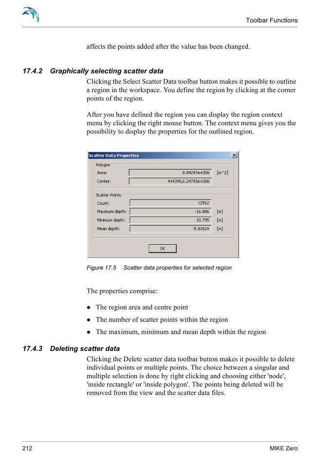
Toolbar Functions

affects the points added after the value has been changed.

17.4.2 Graphically selecting scatter dataClicking the Select Scatter Data toolbar button makes it possible to outline a region in the workspace. You define the region by clicking at the corner points of the region.

After you have defined the region you can display the region context menu by clicking the right mouse button. The context menu gives you the possibility to display the properties for the outlined region.

Figure 17.5 Scatter data properties for selected region

The properties comprise:

The region area and centre point

The number of scatter points within the region

The maximum, minimum and mean depth within the region

17.4.3 Deleting scatter dataClicking the Delete scatter data toolbar button makes it possible to delete individual points or multiple points. The choice between a singular and multiple selection is done by right clicking and choosing either 'node', 'inside rectangle' or 'inside polygon'. The points being deleted will be removed from the view and the scatter data files.

212 MIKE Zero

Prioritization Toolbar

17.4.4 Scatter data editingClicking the Edit scatter data toolbar button makes it possible to modify the z-value of a scatter data point. By activating this tool and selecting either a one or multiple scatter points the user may select to either add a value to the z-value or to modify the z-value. The Selection is done in the same way as the deletion tool.

Finally the editing that has been carried out on to the scatter data will be saved in the corresponding xyz files when the set-up is saved.

Note: Scatter data editing is not covered by the undo and redo functional-ity within the mesh generator.

17.5 Prioritization Toolbar

You use the Area prioritization toolbar to define, modify and delete areas for use in prioritizing scatter values during interpolation.


Define prioritization area

Move area node

Add node to area

Delete area node

Select area

Mesh Generator 213

Toolbar Functions

17.5.1 Prioritization area nameWhen you have selected an existing prioritization area or are creating a new prioritization area, a dialog shows the name of the polygon. You may edit the name.

The names are used for local prioritization of scatter data during interpola-tion, see Prioritize Scatter Data (p. 175).

17.6 Mesh Editing Toolbar

You use the mesh editing toolbar to modify the mesh layout and the node values. After pressing the toolbar icon the pointer enables you to select a node, a face or an element, respectively, for editing.

Note: The changes made to the mesh using the mesh editing facilities are not tracked or saved as a list in the mdf-file. Only the resulting mesh is saved for further reference.


Delete mesh node

Move mesh node

Add mesh node within the existing mesh

Add mesh node at boundary of the existing mesh

Collapse element face. The adjacent elements will automatically be re-tri-angulated

214 MIKE Zero

Mesh Editing Toolbar

Note: The Mesh Editing toolbar is only available when you are in the Mesh Editing mode.

17.6.1 Delete mesh nodeWhen you delete a mesh node you have to specify how to handle the adja-cent elements.

You can choose to re-triangular the adjacent elements or to Make land of the adjacent elements.

Figure 17.6 Retriangulation options when deleting mesh node

In case you specify Re-triangulate the resulting polygon is re-triangulated. An example is shown in Figure 17.7.

Collapse element. The adjacent elements will automatically be re-tri-angulated

Merge triangular elements into one quadrangular element

Edit mesh node properties.

Re-interpolate z-values in selected region

Re-triangulate mesh in selected region


Mesh Generator 215

Toolbar Functions

Figure 17.7 Deleting node: Initial and resulting mesh after re-triangulation

Make landIf the resulting polygon is to be defined as land you have to specify the value of the boundary nodes.

Figure 17.8 Definition of code value in boundary node

The code value for the boundary nodes will per default be 1 (land) but it can be larger, thus indicating an internal boundary.

An example of a resulting mesh changed to land is shown in Figure 17.9.

Figure 17.9 Deleting node: Initial and resulting mesh making land

216 MIKE Zero


17.6.2 Move mesh nodeYou can move a mesh node by selecting and dragging it to a new location. The new location must be within the polygon made up of the elements connected to the node to be moved. Figure 17.10 shows an example.

The z value at the new location is interpolated based on the user default settings for interpolation. The data used as scatter data for the interpola-tion are the values at the mesh nodes.

Figure 17.10 Moving node: Initial and resulting mesh

17.6.3 Add mesh nodeWhen you add a mesh node to the existing mesh you have to specify if you want to re-triangulate adjacent elements.

If yes, then the area with elements adjacent to the element enclosing the new mesh node will be re-triangulated

If no, then only the element enclosing the point will be changed

Figure 17.11 Retriagulation options when adding mesh node

Mesh Generator 217

Toolbar Functions

An example of the resulting mesh using each of the two options is shown in Figure 17.12.

The z value is obtained through interpolation using the user settings. The data used as scatter data for the interpolation are the values at the mesh nodes.

The code value of the mesh node is set to zero i.e. an internal node.

Figure 17.12 Adding node: Initial and resulting meshUpper: Re-triangulating adjacent elementsLower: Triangulation of single element

17.6.4 Add mesh node at boundaryYou can add a mesh node to the boundary of the mesh. An example is shown in Figure 17.13.

The z value of the new mesh node is obtained through interpolation using the user settings. The data used as scatter data for the interpolation are the values at the mesh nodes.

218 MIKE Zero


Figure 17.13 Adding node to boundary: initial and resulting mesh

17.6.5 Collapse element faceWhen a face is collapsed the joined elements may be either triangular or rectangular. As shown in the figures below a triangular element will degenerate into a face element whereas a quadrangular element will degenerate into a triangular element.

The z value of the new mesh node is obtained through interpolation using the user settings. The data used as scatter data for the interpolation are the values at the mesh nodes.

The code value of the mesh node is set to the maximum of the two nodes being collapsed.

Figure 17.14 Collapsing of mesh face for a triangular element

Mesh Generator 219

Toolbar Functions

Figure 17.15 Collapsing of mesh face for a quadrangular element

17.6.6 Collapse elementWhen a mesh element (triangular or quadrangular) is collapsed it takes all nodes in the mesh element and collaps them to the center point of the ele-ment (center of mass) as shown in Figure 17.16.

Note: This procedure may remove up to four mesh elements (five if the collapsed element is quadrangular).

The z value at the new mesh node is obtained through interpolation using the user settings. The data used as scatter data for the interpolation are the values at the mesh nodes.

The code value of the mesh node is set to the maximum of the nodes of the collapsed element.

Figure 17.16 Collapsing mesh element for triangular mesh

220 MIKE Zero


17.6.7 Merge triangular elementsYou can create a new quadrangular element by removing the common face between two triangular elements as shown in Figure 17.17.

Note that element faces can only be removed at the interface between two triangular elements. No interpolation is needed for the new mesh.

Figure 17.17 Merging two triangular elements into one quadrangular element

17.6.8 Edit mesh nodeYou can change the properties for the individual mesh nodes. The options depends on the location of the mesh node.

Inside the model boundary you can modify the location of the mesh node by the (x,y) coordinates and the z value.

At the model boundary can modify the z value and the code value.

Figure 17.18 Editing Mesh node properties

Note: It is possible to select multiple mesh nodes to edit by using the con-text sensitive polygon or rectangular selection tool. In this case the x and the y fields are deactivated.

Mesh Generator 221

Toolbar Functions

17.6.9 Re-interpolate z-values in selected regionYou can re-interpolate scatter data onto the mesh in a selected region. Click the toolbar icon and select a region using the context sensitive poly-gon or rectangular selection tool. The mesh nodes lying within the poly-gon are then highlighted and the interpolation can be carried out for only the selected mesh nodes based on the global settings in the interpolation menu.

17.6.10 Re-triangulate mesh in selected regionYou can re-triangulate a selected region of the mesh. Click the toolbar icon and select a region using the context sensitive polygon or rectangular selection tool. The selected elements and mesh nodes lying within the pol-ygon are then highlighted and the Mesh generation dialog appears (p. 183). After setting the triangulation parameters the re-triangulation can be carried out for only the selected area.

222 MIKE Zero

D A T A V I E W E R

223

224 MIKE Zero

18 INTRODUCTIONThe Data Viewer provides you an environment for inspecting and analyz-ing simulation results obtained from one of the MIKE Zero flexible mesh models. Today MIKE Zero offers the MIKE 21 Flow Model FM, MIKE 3 Flow Model FM and MIKE 21 Spectral Wave Model FM that calculates based on a flexible mesh.

With the tool you can visualize the results as 2D contour plots or as 2D vector field maps, extract values at one or more points and present them in time series plot, presenting results as vertical slices and inspect the raw values as numbers in arbitrarily selected regions. The tool provides you numerous functions for navigating and visualizing the data - e.g. zooming in the horizontal plane, forward and backward spooling in the time dimen-sion and selection horizontal layers in results from the 3D MIKE 3 flow Model FM.

Figure 18.1 Temperature results for an area covering Øresund, Denmark.

Data Viewer 225

Introduction

Although the tool is targeting results files from the MIKE Zero FM mod-els, it provides also some functionality for inspecting and analyzing results obtained with the classic MIKE Zero structured mesh models, e.g. MIKE 21 HD. If you use the Data Viewer for analyzing model results obtained with one of these models, you have to know, that the Data Viewer interpo-late the point values in order to specify the shade color of the element.

Typically you use the Data Viewer for one of the following two reasons:

For analyzing model results - perhaps for trying to identify possible causes for model results or instabilities.

For preparing model results presentations - e.g. animations of tidal wave propagation over the model area, time series plot of current speed in areas of particularly interests.

NOTE: Both the Data Manager and the Data Viewer can be applied to vis-ualize the outline and contents of .mesh and .dfsu files. You may shift the default editor for .mesh and .dfsu files by modifying the file association:MIKE Zero->File->Options->User Settings->File Associations

226 MIKE Zero

19 CONCEPTSYour work with the Data Viewer starts by selecting a simulation results file - typically a file of type .dfsu (result file from one of the FM models). The Data Viewer also accepts files of type .dfs2 (i.e. a file with model results from one of the MIKE Zero structured models) and of type .mesh (a mesh definition file).

After having selected the file you want to analyze your work with the Data Viewer revolves around the use of:

The menu system for defining how and what you want to see from the result file.

The toolbars for accessing often used functionality.

The workspace area context menu - right clicking in the main window - provides you a shortcut for the most used functionality.

The workspace area for specifying time series points, vertical profile routes and node selection for viewing numeric data values.

These elements of the Data Viewer is shown below in Figure 19.1.

Although you can use the Data Viewer to modify the loaded data files, the tool is - as the name also indicates - mainly a browser type of tool. I.e. you will typically not change any data values.

In order for you to get the best out of your work with the Data Viewer, you have to know a few things about MIKE Zero data files:

A data file is organized as a collection of time steps and items.

A time step represents data at specific points in time. A time step in a data file represents data values at a specific point in time.

An item represents a specific physical entity - e.g. surface elevation, temperature etc.

Data files can be categorized as 0-, 1-, 2- and 3-dimensional. The Data Viewer works only with 2- and 3-dimensional files, i.e. files with data that is addressed with 2 or 3 spatial coordinates and one time coordi-nate.

With the Data Viewer you can navigate in the data file by going from time step to step for visualizing e.g. the progression of a tidal wave or from item to item for e.g. correlating tidal wave progression with e.g. salt intru-sion.

Data Viewer 227

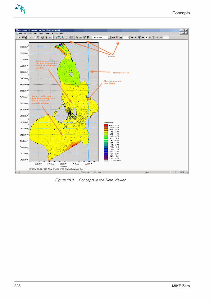
Concepts

Figure 19.1 Concepts in the Data Viewer

228 MIKE Zero

Introduction

20 GETTING STARTED

20.1 Introduction

This chapter guides you through a working session with the Data Viewer. During the session you will try-out a number of the many features the Data Viewer provides you for analyzing and presenting results obtained from the MIKE Zero FM models.

All of the exercises in this getting started guide uses a results file obtained from a 3D simulation of the flow field and transportation of salt and tem-perature in Øresund - the sound between Denmark and Sweden. The simu-lation were originally made during a study undertaken by DHI for the Danish and Swedish authorities in order to assess the environmental impact of construction a link between the two countries. You can read more about this study in the MIKE Zero Flow Model FM Getting Started guide.

The result file used in this example is located in the default MIKE Zero installation folder at

.\MIKE Zero\Examples\MIKE_Zero\DataViewer

The Getting Started example is organized in the following 6 steps:

Step 1 - Visualize salt intrusion in the model areaStep 2 - Viewing the flow fieldStep 3 - Making a time series plot of the salinity concentration at two pointsStep 4 - Creating a Vertical profile of the currentStep 5 - Inspecting data valuesStep 6 - Making a video animation of Salt intrusion

20.2 Step 1 - Visualize salt intrusion in the model area

During this step of the Getting Started example you visualize salt-water intrusion from north in the model area.

Please start MIKE Zero, select File→Open→File. From the presented Select data file dialog you browse to the 3D_flow.dfsu result file. After having selected the file, the workspace area of the Data Viewer displays a contour plot of the first data item in the file extracted at the first time step and top layer. You should see a drawing similar to Figure 20.1.

Data Viewer 229

Getting Started

Figure 20.1 Initial drawing

You can see that the first times step in the data file corresponds to the 6. September, 1997 at midnight and that the file contains 13 time steps in total (counted from 0 to 12) and have 10 layers. You can also see that the first item is the U velocity, which corresponds to the velocity component in the X-direction.

Please select Salinity as a data item from the item selection dropdown but-ton in the toolbar or from the Data menu→Options→Contour dialog. Go to time step 7 (either by using the time step text field in the toolbar or by using the Data→Options→Time dialog). From the View→Display Set-tings... dialog switch to Box Contour. Zoom on the narrow strait at the North end of the area. You should now see something similar to Figure 20.2.

230 MIKE Zero

Step 1 - Visualize salt intrusion in the model area

Figure 20.2 Salt intrusion at the North end of the Sound

Note: You can move around in the model area at the current selected zoom level by use of the scrollbars, e.g. by moving the vertical scrollbar down-wards you will also move the viewport in the data.

Please from the View menu switch to Shaded Contour, impose the mesh, enable a title and a North arrow indicator. Place the North arrow on land area just below the North open boundary. The drawing should then appear as in Figure 20.3.

Data Viewer 231

Getting Started

Figure 20.3 Shaded contours and annotations

Note how much smoother the shading appears.

20.3 Step 2 - Viewing the flow field

This step teaches you to impose a vector field illustrating the current flow in a model area. Again load the 3D_flow.dfsu result file (see Step 1 in the Getting Started guide).

Please select Salinity from the item selection dropdown button in the tool-bar and then select Vectors at element centers from the Data→Option-s→Vector dialog.

In most case time step zero in a results file corresponds to the initial condi-tions of the simulation. This implies that the current velocity is zero in the entire model area and correspondingly no vectors will be drawn. Please go to time step 10 from the time step text button in the Workspace. You should now be able to see some very small vectors representing - and scaled after - the current flow velocities.

In order to better see the vectors please increase the vector length scaling. From the Data→Options→Vector options dialog specify User defined scaling and use 5 as scale factor in both the X- and Y-directions. Figure 20.4 shows the flow field before and after vector scaling.

232 MIKE Zero

Step 3 - Making a time series plot of the salinity concentration at two points

Figure 20.4 Effect of vector scaling

20.4 Step 3 - Making a time series plot of the salinity concentration at two points

In this step you will learn how two use the Data Viewer for extracting data values at user specified points and presenting them in a time series plot.

Please load the 3D_flow.dfsu result file as described in Step 1 of this guide.

You will during this step define two time series location point - one close to the north boundary and one close to the south boundary - and extract data values of salinity and present the data values in a time series plot.

Please ensure that the current selected data item is Salinity. If this is not the case, you can select Salinity as current selection from the dropdown item selection button in the toolbar. Select the Time Series Location button in the toolbar, please notice that cursor changes to a time series icon. Click at a position close to the north boundary and a position at the left part of the south boundary. You should notice that the workspace is updated with a marker at the selected point. Double click the left mouse button outside the model area and the Data Viewer displays the exact location of the point, see Figure 20.5.

Data Viewer 233

Getting Started

Figure 20.5 Point properties dialog

The dialog in Figure 20.5 lets you:

1 Modify the coordinates of the points and

2 Specify whether you want:

To keep the point markers in the workspace,

Remember the locations between invocations of the dialog

Interpolate data values to the exact location of the defined points oruse the nearest point values.

Please keep the settings as they are and click the OK button. The Data Viewer then spools through the file and extracts the requested values. The values will be shown in a time series plot in a window separate from the works space window. You should see something similar to what is shown in Figure 20.6.

234 MIKE Zero

Step 4 - Creating a Vertical profile of the current

Figure 20.6 Time series of salinity

20.5 Step 4 - Creating a Vertical profile of the current

In this step you will learn how to view data values in vertical profiles.


You will during this step define a profile route - ranging from the island of Amager to the island of Saltholm - and generate a vertical contour plot of the distribution of current in the profile.

Please ensure that the current selected data item is Current speed. If this is not the case, you can select Current speed as current selection from the dropdown item selection button in the toolbar. Select the Selection of Ver-tical Profile button in the toolbar and please notice that shape of the cursor changes to a profile. Click at a position on the island of Amager (the larg-est island in the model area and located almost in the middle of the area) and move the mouse to a position on the island of Saltholm (the island slightly to the right of Amager) and double-click. This ends the profile route definition and you will be presented a dialog that shows you the exact coordinates defining the profile route. You can - optionally - modify the coordinates from the dialog as well as you can choose to overlay the workspace area with the profile route. Please accept the settings as they are shown by selecting the OK button.

Data Viewer 235

Getting Started

The Data Viewer extract values along the profile route and downwards. The extracted values will be shown in a window separate from the work-space window as a profile plot. You should end up with visualization sim-ilar to the one shown in Figure 20.7. Please note that contours in Figure 20.7 are drawn as shaded contours.

Figure 20.7 Profile plot

Note: You can with the profile plot view the time evolution of the current distribution by time navigating forward and backward in time - use the Navigate toolbar to either single stepping or playing the data file.

20.6 Step 5 - Inspecting data values

In this step you will learn how to view the exact numerical data values within a user specified area.


You will during this step define a polygon in the area between the islands of Amager and Saltholm (see the previous step for the location of the islands). The reason for this is to inspect the exact values of the current speed within the area.

236 MIKE Zero

Step 5 - Inspecting data values

Please ensure that the current selected data item is Current speed. If this is not the case, you can select Current speed as current selection from the dropdown item selection button in the toolbar. Then Navigate to time step 22 in the data file and finally do a zoom on the area to be inspected. You should now see a workspace area similar to the one in Figure 20.8.

Figure 20.8 Strait between the islands of Amager and Saltholm

Select the Position of Node Selection Polygon button in the toolbar and please notice that shape of the cursor changes to a polygon. Click at a position on the top-right corner of Amager and outline an area encompass-ing the straits between the two islands. Double-click the left mouse button when you are satisfied with the outline. The Data Viewer then opens a dia-log showing you the index numbers of the elements located within the pol-ygon, the current speed at the center of the elements and the x- and y-coordinates at the center point. Depending on your outline the dialog should appear someway similar to the one presented in Figure 20.9.

Data Viewer 237

Getting Started

Figure 20.9 Current speed values

Note: The dialog also lets you specify whether you want the values to be drawn in the workspace area - here, you can select between having the ele-ment numbers and/or data values shown. Selecting the Empty Selection check box empties the current selection and erases any workspace annota-tion. You may use the Calculator to modify the selected element values.

Please ensure that the Display Element Value is selected and the two check boxes are de-selected. Then click the OK button. You should then see a drawing equal to the one shown in Figure 20.8, but with the current speed values shown on top of the contours. Most likely the numbers are located too close to each other for you to be able to read the values. Try to zoom closer to the strait area - you should then see something similar to what is shown in Figure 20.10.

238 MIKE Zero

Step 6 - Making a video animation of Salt intrusion

Figure 20.10 Zoom on the Strait between the islands of Amager and Saltholm

Note: Please be aware that drawing data values on top of the workspace area can take a considerable amount of time.

20.7 Step 6 - Making a video animation of Salt intrusion

The last step in the Getting Started guide is to make a video showing the salt intrusion in the Sound.

Please load the 3D_flow.dfsu result file as described in Step 1 of this guide and ensure that Salinity is selected as the current data item (if this is not the case you can use the Item Selection dropdown button in the toolbar to select the Salinity Item).

Please from the Video→Properties dialog specify the name of the file to hold the video and specify a frame rate of 10 frames per second, see Figure 20.11.

Figure 20.11 Setting Video generation properties

Data Viewer 239

Getting Started

Select the OK button and back in the Workspace area make sure that the current time step number is 0 (use the time step button in the Navigate toolbar if this is not the case). Press the Video Forward button in the Navi-gate toolbar to initiate the video generation. You will then be given the option to compress the video output file. The workspace window will be updated during the video recording.

Note: Please be aware that video generation can take a considerably amount of time.

A message box, see Figure 20.12, will inform you when the video genera-tion has ended.

Figure 20.12 Video generation notification

You can distribute video like this one to e.g. your customers. They will be able to view the video with most modern media players like e.g. Microsoft Media Player. Figure 20.13 below shows the above-generated video loaded in Microsoft Media player.

Figure 20.13 Salt Intrusion in Microsoft Media Player

240 MIKE Zero

File Menu

21 REFERENCE GUIDEThe Data Viewer provides you an environment for inspecting and analyz-ing simulation results obtained from one of the MIKE Zero flexible mesh models.

21.1 File Menu

The File Menu provides functionality for opening, closing and saving files, and for accessing printer related utilities.

21.1.1 File/New MenuYou use the File→New menu to create a new workspace for viewing and analyzing model results. Selecting this menu provides you with a file selection box you use to navigate to the result file you want to analyze. You can select files with the following extensions:

.dfsu - simulation results from the MIKE Zero FM models.

.dfs2 - MIKE Zero type 2 data file - typically results from the MIKE Zero 2D simulation modules.

.mesh - flexible mesh generated by the MIKE Zero Mesh Generator tool.

21.1.2 File/Open MenuYou can use this menu to open a MIKE Zero FM result file (file type .dfsu) for viewing and analyzing model results.

Additionally you can open a .frv file. A .frv which contains settings from a previous work session with the Data Viewer, e.g. a reference to the results file and like zoom level, item selection, vector scaling etc.

21.1.3 File/Save (Save As)You can save your Data Viewer settings in a .frv file. This file will contain a reference to the results file plus various settings like zoom level, item selection, vector scaling etc.

21.2 Edit Menu

The Edit menu is currently not used by the Data Viewer tool.

Data Viewer 241

Reference Guide

21.3 View Menu

The View provides you with functionality for customizing the workspace area by e.g. overlaying it with geographical information like a longi-tude/latitude net, a North arrow and with general annotation. You can e.g. annotate the area by:

A data title giving the name of the currently loaded data file

Changing the used contouring algorithm

Zoom level

Etc

21.3.1 Coordinate OverlaysThis menu makes it possible to overlay the workspace area with a geo-graphical net showing the longitudes and latitudes, a map projection grid and an arrow pointing towards true North.

Map ProjectionYou can add or remove a map projection net in the display.

You can select which map projection net to overlay. Per default the dis-played map projection net is defined as in the data file.

North ArrowYou can add or remove a north indicator in the display.


21.3.2 Display Settings By default the Data Viewer shows a shaded contour plot of the first item (and first time step) in the data file. Alternatively other contouring algo-rithms can be applied by editing the Contour Type.

The plot display can furthermore be defined by Isolines, Miscellaneous settings and Common view properties.

Contour TypeYou can define the way contours are displayed. The contour is defined by a Primary option that defines the contour type and Secondary options that depends on the primary option.

242 MIKE Zero

View Menu

Primary optionsBox Contour Each grid cell is given a colour according to the value in the cell.

Box Contour with transparencyEach grid cell is given a colour according to the value in the cell. Secondary Options: No. 1

Shaded ContourThe grid is covered with colours indicating the values in the cells, a smooth surface is used. The land values will always be displayed in green.Secondary options: No. 2 or No. 3 or No. 4 + No. 1

No Contour Used in connection with background overlays. The bathymetry will not be shown.

Secondary options1 Transparency

Used in connection with background overlays the value defines the transparency of the layer.

2 Copy ColoursThe colours indicate the values in the cell.

3 Copy Colours with TransparencyThe colours indicate the values in the cell, one colour is fully transpar-ent (usually white).

4 Blend coloursAll colours are transparent with a user-defined transparency (second-ary option 2) and one colour is fully transparent (usually white).

Isolines

IsolinesThis check box toggle between showing or hiding a layer with isoline information. The isolines represent line with constant data values.

The isolines are created following the same algorithm as is used for true (i.e. not box) contour plots.

Draw labels Apply labels to the isolines. either as transparent, opaque or framed opaque.

Data Viewer 243

Reference Guide

Properties for isoline labelsThe maximum number of isoline lables, check for colliding labels and removal of adjacent identical labels can be controlled here

Miscellaneous

Element meshThis check box toggle between showing or hiding a layer with the mesh used in the model simulations.

BorderThis check box toggle between showing or hiding the boundary lines in the model area.

Color legendThis check box toggle between showing or hiding a color legend. The color legend is drawn to the right of the workspace and shows the correla-tion between colors and data values.

The scale used by the Data Viewer when generated the color legend can be taken from the data range in the current zoomed area, the current layer or from the whole data item. You select between these options from the Colors→Auto Scale Type menu.

TitleThis check box toggle between showing or hiding a title on the plot. The title is drawn above the workspace and shows the name of the result file.

White backgroundThis check box toggles between showing the background by white or gray color.

Color dried land as backgroundThis checkbox enables delete values in the data to be shown by the back-ground color. This is especially useful when presenting results from flood-ing simulations.

Common view properties

Position of attached overlaysControls whether multiple color legend overlays should be stacked from the bottom and up or stacked from the top and down.

244 MIKE Zero

View Menu

21.3.3 VectorsThis menu toggle between showing or hiding a layer with the calculated flow velocity, the flow velocity is shown in the form of a vector field. The Data Viewer will in most cases be able to select the right information from the result file in order to create the vector field, this is always the case with e.g. results file from the MIKE Zero FM models.

In case the Data Viewer for some reasons does not have the information necessary for selecting the flow velocity information, you can specify the items in the result file that contains the flow velocity components. You do this from the Vector entry in the Data Viewer dialog, select the Data→Op-tions menu.

21.3.4 Axis AnnotationThis enables you to toggle between showing or hiding the workspace axes, i.e. the coordinate axes.

21.3.5 Value at CursorThis enables you to toggle between showing or hiding the value of the individual element.

21.3.6 Zoom inThe Zoom In menu gives access to a rubber band you can use to select a sub-area to work with. You use the rubber to define the sub-area - with the band present, you outline the area by pressing the left mouse button and dragging the mouse. When you release the button, the Data Viewer will zoom to the specified area.

21.3.7 Zoom to CoordinatesWith the Zoom to Coordinates menu you can define the zoom area by specifying the coordinates at the lower left and upper right corner of the area.

21.3.8 Zoom OutThe Zoom Out menu resets the zoom level to the full workspace area.

21.3.9 Fixed Aspect RatioThis menu toggle between drawing in fixed aspect ratio or not. With Fixed Aspect Ratio enabled the workspace area will be drawn using the same scale for both x- and y-coordinates. Clearing Fixed Aspect Ratio results in a workspace area that fills the entire editor window.

Note: It is not possible to enable Fixed Aspect Ratio whenever the ratio between the two axis is less than 0.02.

Data Viewer 245

Reference Guide

21.3.10 Export GraphicsWith the Export Graphics menu you can copy the workspace area as an image to the clipboard or directly save it in a file as a bitmap or Windows metafile. This is mainly used when preparing presentations or for import-ing illustrations in reports.

21.3.11 FontThis menu lets you select the font to use for drawing text in the workspace area.

21.3.12 ToolbarThe Toolbar menu gives access to a toolbar selection dialog.

Note: you cannot deselect the Data Viewer specific toolbars.

21.3.13 StatusbarThe Statusbar menu toggles between showing or hiding the MIKE Zero statusbar.

21.4 Data Menu

You use the data menu for changing the aspect of the data that is visual-ized. E.g. you can from the menu select one or more points in the data and have the Data Viewer to generate a time series plot of the values in the specified point or points. Or you can use the data menu to select the time step or data item that shall be visualized in the workspace area.

21.4.1 OptionsThe options menu provides you a number of dialogs from where you can select and specify different aspects of the data to be visualized.

246 MIKE Zero

Data Menu

Figure 21.1 Options dialog

Specifically you can use the Options dialog to set:

The specific time step in the data file that shall be visualized.

The item in the data file that shall be visualized.

Enabling or disabling of drawing the mesh and or model area bounda-ries.

Enabling or disabling of vector drawing. You can also specify the items from the data file that constitute the vector field.

Vector scaling options.

Different textual annotation of the workspace area.

Time You use this dialog to specify the discrete time step from the data file that you want to visualize in the workspace area.

Data Viewer 247

Reference Guide

Figure 21.2 Time options dialog

Note: You can also use the Goto Time Step button in the Navigate toolbar to reach this functionality.

You can also specify a jump value to be used when scrolling forward and backward in the data file.

LayersYou use the Layers dialog to specify the vertical layer from where the data for visualization shall be taken. You can either specify a layer based on sigma coordinates or on an interpolated Z coordinate.

All of the MIKE Zero 3D FM models use Sigma coordinates - i.e. dimen-sionless transformed coordinates - for the representation of the vertical axis. In the transformed coordinate system the distance between sigma layers are constant over the model area - but when converted back to phys-ical values (e.g. meters) the spacing is not equidistant.

248 MIKE Zero

Data Menu

Figure 21.3 Layer options dialog

If you select Sigma layer you shall specify the layer number while you with Interpolated Z-values specifies z-coordinate.

Note: You can also use the Goto Layer button in the Navigate toolbar to reach this functionality.

Contour You use this dialog to specify the item from the data file you want to visu-alize in the workspace area.

Figure 21.4 Contour Options dialog

Data Viewer 249

Reference Guide

The dialog lets you select amongst the items found in the data file for con-tour visualization. You can also from this menu specify the type of con-touring and whether you want enable or disable contour drawing.

See section 21.3.2, Display Settings for an explanation of the different contour options.

Note: You can also use the Item selection dropdown box in the Navigate toolbar and the View Menu to reach this functionality.

Mesh You use this dialog to enable or disable the drawing of the model mesh and/or model boundaries.

Figure 21.5 Mesh Options dialog

Note: You can also use the View menu and the workspace context menu (right clicking in the workspace area) to reach this functionality.

Vector This dialog enables you to overlay the workspace area with a vector field illustrating the flow field within the model area. The Data Viewer uses two items from the data file in order to draw the flow field. With results files from all the MIKE Zero FM models the data viewer knows the items for use with vector drawing, with other types of files, however, you might have to specify the items to be used. In such case you use the Vector dia-log to select the items.

250 MIKE Zero

Data Menu

Figure 21.6 Vector Options dialog

The dialog also lets you specify how to place the vectors and - in case you select the vectors to be interpolated to a structured mesh - how to distrib-ute the vectors in the workspace area.

Note: You can also use the View menu and the workspace context menu (right clicking in the workspace area) to reach this functionality.

Vector optionsYou use the options on this dialog to specify the scaling of the vectors illustrating the flow field. You can either let the Data Viewer scale the vec-tors or you can specify your own scaling.

Figure 21.7 Vector scaling Options

Data Viewer 251

Reference Guide

If you want to make your own vector scaling you shall specify the length of the x- and y-components measured in average node distance corre-sponding to 1 m/s.

Text annotationsYou use this dialog to specify textual annotation of workspace area.

Figure 21.8 Text Annotation Options

You can e.g. specify a title that will be drawn on top of the workspace area, coordinate axes text and other informational text.

Note: You can also use the View to reach part of this this functionality.

21.4.2 Vertical Profile by CoordinatesIf the data file you work with includes 3-dimensional data values, you can use the Vertical Profile by Coordinates dialog to visualize the data values in a vertical plan. The vertical plane is defined by defining a polyline in the horizontal plane - you define the polyline by entering the x- and y- coordinates oat the corners of the polyline in the dialog.

252 MIKE Zero

Data Menu

Figure 21.9 Vertical Profile Definition

After confirming the coordinates by selecting the OK button, the data in the vertical plane will be visualized in a separate window as a contour plot.

You can enable or disable a graphical representation of the profile route in the workspace.

Note: You can also specify the polyline by using the Position of vertical profile toolbar button.

21.4.3 Time series by CoordinatesThe Time Series by Coordinates dialog lets you specify one or more points in the workspace area. The maximum number of points to extract is 100.

The Data Viewer extracts values at each time step in the data file and presents them in a time series plot.

Data Viewer 253

Reference Guide

Figure 21.10 Time Series by Coordinates Specification

You have to be aware that with large data files, it might take some time for the Data Viewer to extract the values and present them graphically.

You can specify whether the Data Viewer shall remember the Time Series locations between activation of the dialog and whether the location of the extracted time series shall be shown in the workspace.

Note: You can also specify the points by using the Position of time-series toolbar button.

21.4.4 Selected PointsIn some situations you might want to know the exact numeric value at one or more points within the model area. You use the Selected Points dialog box to specify one or more points at which you want to know the data val-ues.

254 MIKE Zero

Data Menu

Figure 21.11 Selected Points Specification

The data values will both be shown in the dialog and - optionally - in the workspace area In case you prefer to view the numbers in the workspace area, you will most often have to zoom very close to the area with the selected points.

You can also select to see the element numbers in the workspace area by selecting the Display Element No. check box. To remove data values from the workspace area, you re-select this dialog and select the Empty selec-tion check box.

Note: You can also specify the points by using the Position of node selec-tion polygon toobar button.

CalculatorThe calculator can be used to assign values to a dataset. It can be done in terms of a simple value or as an expression. Table 21.1 gives an overview of the functions. It lists the function names, the number of arguments and a brief description.

Table 21.1 Overview of functions in calculator

Name Argc. Explanationsin 1 sine function

cos 1 cosine function

Data Viewer 255

Reference Guide

Table 21.2 lists the default operators supported.

tan 1 tangens function

asin 1 arcus sine function

acos 1 arcus cosine function

atan 1 arcus tangens function

sinh 1 hyperbolic sine function

cosh 1 hyperbolic cosine function

tanh 1 hyperbolic tangens function

asinh 1 hyperbolic arcus sine function

acosh 1 hyperbolic arcus cosine function

atanh 1 hyperbolic arcus tangens function

log2 1 logarithm to the base 2

log10 1 logarithm to the base 10

log 1 logarithm to the base 10

ln 1 logarithm to the base e (2.71828...)

exp 1 e raised to the power of x

sqrt 1 square root of a value

sign 1 sign function -1 if x<0; 1 if x>0

rint 1 round to nearest number

abs 1 absolute value

Table 21.2 Overview of operators in calculator

Operator Meaning= assignement*

+ addition

- subtraction

* multiplication

Table 21.1 Overview of functions in calculator

Name Argc. Explanation

256 MIKE Zero

Video Menu

21.4.5 Add and remove layersThis menu lets you import image files and use them as background in the workspace area. You have to specify the path of the images and the posi-tion of the images relative to the workspace area. The latter is defined by specifying the coordinates to the image origin (lower left corner) and the extent of the image in meters or degrees.

Note: You specify the image origin and extent by clicking the Edit button in the Image Manager dialog. In the Overlay Manager dialog you can specify which layer to display and the display order.

21.5 Video Menu

You can use the video menu to set options for generation an animated video of the data.

21.5.1 PropertiesThis dialog lets you specify the filename of the video output.

Figure 21.12 Video Properties

The video file will be generated as an AVI file. You can use e.g. Microsoft Media Player to play the file. From the dialog you can also specify the frame rate of the video, i.e. the speed with which the file shall be played.

Note: The generation of the video is not initiated from this dialog. You will have to use either the Video forward or Video reverse toolbar buttons

/ division

^ raise x to power of y

Table 21.2 Overview of operators in calculator

Operator Meaning

Data Viewer 257

Reference Guide

to actual generate the video. You shall be aware that generation of a video can take a considerable amount of time.

21.6 Colors Menu

You use the Colors menu to specify how to generate the color legend and to define a color palette for the contour drawing.

21.6.1 Auto Scale TypeThe Auto Scale Type menu lets you select between three different ways to generate the color legend:

Current Zoom - this option generates the color legend based on the minimum and maximum data values from the data at the current time step and within the current zoom level (the area you have zoomed to).

Current Layer - this option generates the color legend based on the minimum and maximum data values from the data at the current time step and current vertical layer, i.e. at the same Z (or sigma) coordinate.

All Data - this option uses the minimum and maximum values from all time steps and all layers when generating the color legend.

21.6.2 New PaletteThis menu lets you define a custom palette. The palette is used for select-ing the specific colors representing data value ranges.

21.6.3 Save Current PaletteThis menu lets you save a custom defined palette.

21.6.4 Edit Current PaletteThis menu lets you edit a custom defined palette.

21.6.5 Open PaletteThis menu lets you open and read a previous defined palette.

21.7 Time series context menu

You can use the time series context menu (right-click in the time series window) to change zoom level of the time series plot, to save the graphics as a bitmap or a metafile and to save the extended data value as a dfs0 file.

258 MIKE Zero

Time series context menu

21.7.1 Select Item for ExportYou use this dialog to select the items, i.e. values from specific points, you want to save in the dfs0 file.

Data Viewer 259

Reference Guide

260 MIKE Zero

Zoom Functions

22 TOOLBAR FUNCTIONSThe following describes the main editing functions that are available to you from the toolbar.

22.1 Zoom Functions

Figure 22.1 Zoom functions toolbar

You can Zoom-in, Zoom-out and go to Previous-zoom and Next-zoom. You can recall all available previous and next zooms. If the buttons are grayed-out there are no previous or next zooms available.

These functions are also available from the workspace context menu (i.e. right-clicking in the workspace area).

22.2 Data Functions

Figure 22.2 Data functions toolbar

You use the data functions to:

Select points for time series generation

Select position for visualizing the data values in a vertical profile

Select position of node selection polygon for inspecting the numeric data values.

Data Viewer 261

Toolbar Functions

22.3 Navigation Functions

Figure 22.3 Navigation toolbar

You use the navigation functions to navigate in the data file. You can:

Select the data item to visualize

Select the horizontal layer to visualize. Note: The MIKE Zero FM models all work with Sigma coordinates in the vertical dimension. This implies that the distance between layers measured in physical units (e.g. meters) is not constant.

Select the time step in the data file to visualize.

Generate a video from the data file.

Table 22.1 Icon Description for Data functions toolbar

Icon Description

Use this function to deselect a previous selectedfunction.

Use this function to select points for time series generation.

Use this function to specify a polyline for verticalprofile generation.

Use this function to select a polygon for inspection of numeric data values.

262 MIKE Zero

Navigation Functions

Table 22.2 Icon Description for Navigation functions toolbar

Icon Description

Use this function to select the item from the data file to visualize.

Use this function to select the layer just above the cur-rent layer for visualization.

Use this function to select the layer just below the cur-rent layer for visualization.

Use this function to toggle between layer selection based on sigma value or z-coordinate.

Use this function to select the layer from which data shall be visualized. If Sigma-based selection is enabled you specify a layer number otherwise you specify the z-coordinate.

Use this function to visualize the data from the first time step in the data file.

Use this function to visualize the data from the time step just before current time step.

Use this function to generate a video file by automati-cally going backward in the data file. Note: You specify the name of the vide file from the Video→Properties menu

Use this function to automatically update the visualiza-tion by going backward one time step in the data file. No video file is generated.

Use this function to stop video generation or automati-cally playing the data file.

Use this function to automatically update the visualiza-tion by going forward one time step in the data file. No video file is generated.

Use this function to generate a video file by automati-cally going forward in the data file. Note: You specify the name of the vide file from the Video→Properties menu

Use this function to visualize the data from the time step just after current time step.

Data Viewer 263

Toolbar Functions

Use this function to visualize the data from the last time step in the data file.

Use this function to select the time step number in the data file from where the data shall be visualized.

Table 22.2 Icon Description for Navigation functions toolbar

Icon Description

264 MIKE Zero

D A T A M A N A G E R

265

266 MIKE Zero

Operation and navigation

23 DATA MANAGERThe Data Manager is a utility for managing (create, edit, copy, etc) Dfs data files associated with the DHI Software product series.

Data Manager supports the flexible mesh (FM) data files: 2D and 3D .dfsu files, .mesh files and to some degree 2D and 3D grid files (dfs2 and dfs3 files).

The Data Manager can be accessed by right-clicking the file and choosing the option ‘Open with’ Data Manager if the Data Manager has not been associated as a default editor for the file.

Note that the Data Manager is designed to update files. Do take a backup of important simulation files, before loading it into the Data Manager. When changes to a file are saved to disc, and the Data Manager closed down, there is no undoing of changes.

23.1 Operation and navigation

You operate the Data Manager from the main menu, the tool bar icons, or by right-clicking on the graphical view.

By pressing and holding the shift button and then pressing and holding the left mouse button, you can pan/move the view. By pressing and holding the shift button and role the mouse wheel, the view will zoom in/out.

To the right of the graphical view, there is a table of "Element id" and "Value". You can mark individual element values by using shift/Ctrl and left mouse button, or you can mark all values by clicking the "Value" header. These values can be copy-pasted into other applications (text edi-tors, Excel etc.). Similarly, data can be copy-pasted back into the table from text editors, Excel or others.

Right clicking in the graphical view, you get the context menu, see Figure 23.1. The context menu contains options to zoom, pan, view mesh and other visual options, herein Selection and Cropping of data.Unselecting "Shaded contours" will show box contours instead.

Data Manager 267

Data Manager

Figure 23.1 Context menu

23.1.1 SelectionTo select/highlight certain elements, right click the graphical view, choose "Select area". Then by repeatedly left clicking the mouse in the graphical view, you select a polygon. By double clicking, the polygon selection ends, and all elements having center within the polygon will be selected/highlighted. To remove selection/highlighting, right click and choose "clear selection" from the context menu.

23.1.2 CroppingHaving selected one or several areas, you can crop the data in two ways:

Crop to selectionHere you keep the data that are selected

Cut out selectionHere you keep the data that are not selected

NOTE: The Data Manager is designed to update files. When cropping or cutting data there will be given no option to save the result in a new file, thus keeping the original file untouched. Do take a backup of important simulation files, before loading it into the Data Manager.

268 MIKE Zero

File

23.2 File

You may create, open and save files from the File drop-down menu.

NOTE:Any modifications you have made to your file after opening or creation are only saved after you have selected ‘Save’ or ‘Save As’ from the File menu. However, when using Cut/Crop the modifications are saved imme-diately.

23.2.1 New fileCreating a new data file requires specification of the spatial properties of the mesh, the time axis and the item(s). Thus a wizard of three steps must be followed to create a new file.

NOTE: You have to save the new file by a filename before you can con-tinue to edit the data values in the file.The new file will have one time step only.

Spatial InformationFirst you define the spatial properties of the file by selecting a file to import the mesh from.

This can be a mesh file generated by the Mesh Generator or an existing dfsu-file. If the selected file is a 3D dfsu file, the layers will be imported, but not editable and constant in time, corresponding to the initial time step in the 3D file.

Data Manager 269

Data Manager

Figure 23.2 New file wizard page 1 - define spatial grid

Time axis informationThen you specify the time axis type. You have five options:

Undefined

Equidistant - no explicit start time

Non-equidistant - no explicit start time

Equidistant - explicit start time

Non-equidistant - explicit start time

If selecting an equidistant axis, you have to specify the time step and time step unit. If selecting an explicit start time you have to define the date and time of the first timestep.

NOTE: It is not possible to create a file with more than one time step.

270 MIKE Zero

File

Figure 23.3 New file wizard page 2 - define time axis

ItemsFinally you define the items in the file.

For each item, you must specify its name, type and unit. You may add, edit and delete item information before you save the file by pressing `Finish'. When `Finish´ has been pressed, it is no longer possible to add more items.

Data Manager 271

Data Manager

Figure 23.4 New file dialog 3 - define item(s)

23.2.2 Open fileThe default editor/viewer for dfsu data files can be set to either the Data Viewer or the Data Manager via the User Settings in the MIKE Zero shell.

If the dfsu file is contained in a MIKE Zero project, you can open an exist-ing file in the Data Manager, even if the default editor is set to the Data Viewer, by right-clicking the file in Project Explorer and choose the option ‘Open with...’ Data Manager. The data are then immediately pre-sented in the Data Manager dialog where data can be viewed and edited both in a graphical and in a tabular view.

23.3 Edit

23.3.1 CalculatorYou access the Calculator from Edit on the main menu.

The Calculator can be used to assign/edit values of the current dataset. It can edit the currently selected item of the dataset. The assignment can be done in terms of a simple value or as an advanced expression. You can decide to assign to

272 MIKE Zero

Edit

All values in the dataset or a user defined subset.

The currently selected timestep or all timesteps.

The user defined subset must be selected in the DataManager before enter-ing the Calculator.

NOTE: When working on large datasets, significant increase of computa-tional speed can be gained by using the foreach special function when the expression only contains one item, see Special Functions (p. 277).

Figure 23.5 Calculator dialog

VariablesThe list shows variables that can be used in an expression. Default is listed the CurrItem, the currently selected item of the dataset being edited.

You can add more items from the same file, and items from other files. The Calculator automatically handles a number of issues.

Data Manager 273

Data Manager

Adding items from the same fileItems need not have the same units. The Calculator automatically converts between units of same type, i.e., you may add different units of length as meters and feet, and the result will be as expected.

NOTE: The resulting Calculator-expression must have the same unit type as the current item, unless the function void() is used.

Adding items from another fileThe files need not to be based on the same mesh. Necessary interpola-tion is performed in the added items, when the meshes do no match.Note that even very small differences will imply interpolation. See also Calculation mode (p. 275).

The files need not have the same temporal definition. Necessary inter-polation in time is performed in the added items, when the timesteps do no match.

The files need not cover the same geographical area. The full expres-sion is only applied in the intersecting area. In areas not covered by the added items, undefined or zero values will be used instead.

The coordinate system projections need not to match. All coordinates are transformed into the system of the current file.

NOTE: In case of 3-dimensional files the calculator expression considers the vertical position of the cell as well.If the files are exactly the same in the vertical, as well as being the same horizontal mesh, the mesh values are used directly in the expression. However, if the mesh resolution in the two files differ, either horizontal or vertical, the variables applied will be based on the centre cell value for the individual mesh elements. This is found by interpolation considering the values in the adjacent layers and elements. See also Calculation mode (p. 275).

Output Options

Timestep selectionThe expression can be applied to timesteps in the following ways:

Apply to only selected timestep of current item.

Apply to all timesteps of current item.

274 MIKE Zero

Edit

Apply to all resulting timesteps. This means that if the time definition of an added item goes beyond the final time of the current item, timesteps will be added to the current item and the file, thereby increasing the number of timesteps in the cur-rent file.

Area selectionIf a number of elements are selected in the DataManager before entering the Calculator, you can specify whether the expression is applied to the selected elements, or all elements in the current file. Default is "only selected area" if some area is selected, and "all elements" if no area is selected.

When operating on a variable, the function or operator will be applied to all values of the variable unless otherwise stated.

You may limit the data for editing by defining certain time steps and/or selected area.

Calculation modeYou have the option to force the calculations to be carried out in interpo-late mode instead of using discrete values values as per default. This is especially useful when you perform complex computations and the meshes are different.

ExpressionThe Calculator allows you to compose your own expressions that can be used to assign or modify values of the current item in the data set. All operators and functions can operate on either constants or variables.

All operators and functions will be applied to elements of the current item individually. This means that all/selected values of the current item will be updated, but the spatial description will remain unchanged.

The usual Mathematical Functions and Operators can be used, and works in the traditional manner. Furthermore, some Special Functions are defined.

Units are handled in the expression. If one item of unit [m/s] is multiplied with an item of type [s], the resulting unit is [m]. A variable with unit [m/s] can not be added to a variable of unit [m].

NOTE: The entire expression must return the same unit as the current item. To circumvent mismatching units, either the convert() or the void() function must be used.

Data Manager 275

Data Manager

Mathematical FunctionsBelow you will find a table with a list of the mathematical functions you can choose between and which result they return.


Function Evaluation

abs(x) The absolute value of x

sin(x) The sine of x Note: x is given in radians

cos(x) The cosine of x Note: x is given in radians

tan(x) The tangent of x Note: x is given in radians

sinh(x) The hyperbolic sine of x

cosh(x) The hyperbolic cosine of x

tanh(x) The hyperbolic tangent of x

ceil(x) Smallest integer value greater than x

floor(x) Largest integer value less than x

exp(x) Exponential value of x

log(x) Natural logarithm of x

log10(x) The base-10 logarithm of x

sqrt(x) The square root of x

max(x,y) maximum value (returns the bigger value of x or y)Note:

x and y must be scalars, they cannot be items.Use the foreach() function to apply on items:foreach(it in CurrItem, max(it, 0.6))

min(x,y) minimum value (returns the minor value of x or y)Note:

x and y must be scalars, they cannot be items.Use the foreach() function to apply on items:foreach(it in CurrItem, min(it, 0.6))

276 MIKE Zero

Edit

Special FunctionsA number of special functions are available in the Calculator:

undefined()E.g. undefined(arg).

Returns true/false indicating the state of arg.Does not check each value in a variable. This is because the variable itself can be flagged as undefined.See the foreach(<it> in <variable>, expression) construct for explicit value iteration.

convert()E.g. convert(value, eumUnit)

Returns a copy of <value> converted to the requested eumUnit.

if()E.g. if (test_expression, then_expression, else_expression)

Evaluates <test_expression> as true/false, and then executes either <then_expression> or <else_expression>.

foreach()E.g. foreach(<iteratorname> in <var>, expression)

Defines <iteratorname> as an iterator variable for the variable <var>. This iterator can then be used in <expression> as <iteratorname>.Eg. foreach(it in Var1, it+5), which will add 5 to all values in Var1.

In all cases where an expression is to be applied to all values in a variable, the foreach operator will be much faster than the corresponding simple expression.Eg. foreach(it in Var1, it+5) will execute much faster than the simple (but equivalent) expression Var1+5.

When performing a calculation on all values in a variable, but disregard-ing undefined values it is necessary to use the foreach operator.Eg. foreach( it in Var1, if (undefined(it), it, it+5) ), will add 5 to all values in Var1 that are not undefined.

When performing a max/min calculation it is necessary to use the foreach operator, e.g. foreach(it in Var2, max(it,0.7)).

Data Manager 277

Data Manager

void()E.g. void(value)

Returns a copy of <value> without any unit attached.

OperatorsBesides the normal operators such as plus, minus, multiply and divide you may use delimiters and relation operatores as given below.

23.3.2 InterpolateThis feature interpolates a given item spatially. The interpolation will replace originally undefined or delete values with interpolated values.

23.3.3 Mark and restoreMark and restore provides a kind of version control and can be used to undo changes made to a dataset.

When modifying a dataset, you may want to mark the current version, to be able to recognize it at a later time. You can continue editing the file, make as many marks as necessary. If you at some point find out that a pre-

Table 23.2 List of operators

Operator example Evaluation

v1 + v2v1 - v2v1 * v2v1 / v2

Ordinary binary operators

v1^ pow Power operator. Eg. v1^pow raises v1 to the power of pow

v1 == v2v1 < v2v1 > v2v1 <= v2v1 >= v2v1 <> v2

Ordinary binary comparison operators

- the ‘not equal’ operator <> can also be specified as !=

- v1 Unary minus operator

( ) Parenthesis can be used for explicit expression grouping

278 MIKE Zero

View

vious version of the dataset is better, you can restore the data from that version.

When you restore a previous version, all future marks/versions are deleted.

Every time a calculator expression is executed, a mark is automatically created.

23.4 View

You may select which item, time step and layer to view and edit from the View drop-down menu.

23.4.1 ItemsYou select the item to view by choosing between the available data items in the dataset.

Figure 23.6 Select item dialog

23.4.2 Add/Remove imagesIt is possible to add images to the graphical display. The order of the dis-played layers can be defined in the overlay manager.

23.5 Tools

23.5.1 StatisticsThis tool calculates the statistics of the selected item in the dataset.

Data Manager 279

Data Manager

The output will be a dataset file with only one time step, containing three items:

1 Statistical minimum

2 Statistical maximum

3 Statistical mean

23.5.2 Extraction

Figure 23.7 Data Extraction utility

In the Data Extraction tool you can extract data from a dfsu file.

The possible dimension and definition of the output is dependent on the dimension of the input dfsu file.

You may extract data in three dimensions:

Point

Column (for 3D data files only)

Profile

280 MIKE Zero

Tools

Figure 23.8 Illustration of output types when extracting data from dfsu filesRed : 2D dfsu file, Green: 3D dfsu file

PointThe output from extracting data in a point is a dfs0 file.

You may define the location in two ways:

CoordinatesHere you define the xy(z) coordinates of the extraction point directly.

Digitize from graphical viewHere you mark the position of the point on the graphical view.You define the z-coordinate of the extractio point directly.

ColumnThe output from extracting data in a column is a dfsu file. The dfsu file contains the values from the layers in the vertical, defining element number 1 as the bottom layer, and increasing in number towards the water surface.

You may define the location in two ways:

CoordinatesHere you define the xy coordinates of the extraction point directly

Digitize from graphical viewHere you mark the position of the point on the graphical view

Note: this option only works for 3D data files.

ProfileThe output from extracting a profile depends on the dimension of the input dfsu file. In case the file is a 2D file, the output is a dfs1 file showing the

Data Manager 281

Data Manager

values along a line. In case the file is a 3D file, the output is a dfsu file showing the values in the vertical along a line. You may define the loca-tion in two ways:

Digitize from the graphical viewHere you mark the position of the line on the graphical view

Load from .xyz fileHere you specify the name of a .xyz file (z-value is not used).

An additional option is to interpolate the profile line to follow the nearest segment list, i.e. a line through the node values as displayed in Figure 23.9.

Figure 23.9 Extraction of data along profile line from (0,50) to (1000,50)Upper: element meshMiddle: default extraction line Lower: extraction line when including nearest segment list

23.5.3 Export to xyz

Figure 23.10 Export element values to xyz file

282 MIKE Zero

Examples

This tool export element values from the file to ascii file(s) with extension xyz.

For each selected item and time step a separate file is generated. The indi-vidual files are named by the item description and time value, e.g. ‘Sur-face elevation_01-01-2004_01-20-00.xyz’ for the item ‘Surface elevation’ at the time step ‘01-01-2004 01:20:00’.

A generated output xyz file contains four columns:

1 x-coordinate

2 y-coordinate

3 z-coordinate (in case of 2D files this is the bathymetry value)

4 element value

23.6 Examples

The following describe some examples of use of the Data Manager.

23.6.1 Comparing simulation resultsIf you have several simulations of the same area, the Data Manager can compare the results.

Assume we want to compare one item as, e.g., surface elevation from the two files: data1.dfsu and data2.dfsu. There are two ways of accomplishing this: A fast procedure and a "reusable" one.

The fast procedure can be applied, when you want to see the difference here and now, but you do not need to save the difference to a file. The reusable procedure will save the difference to a new file.

The fast procedure1 Load data1.dfsu in the Data Manager.

2 Select the item and timestep that you wish to compare.

3 Start the Calculator.

4 Add the corresponding item from data2.dfsu as a new variable.

5 In expression, type: CurrItem-Var2

Data Manager 283

Data Manager

6 We need to specify whether we want to compare all timesteps, or just the current one. Then press Calculate.

Now the current item will be the difference between the two.

NOTE: Do not press save, since the current item will be overwritten with the newly calculated data, and the original data in data1.dfsu will be lost.

The reusable procedureThis is the procedure when you want to save the result in a third file.

1 From the menu, select "file", "new", "file" and find the Data Manager. This will start the "New file wizard".

2 Select "import 2D or 3D dfsu file", and choose either data1.dfsu or data2.dfsu. This will be the mesh that the comparison will be made on. Click "next"

3 Select an equidistant time axis - no explicit start time. Specify a timestep corresponding to either of the data1.dfsu, data2.dfsu files.

4 Add a new item corresponding to the item you wish to compare, e.g., surface elevation. Specify type and unit. If you wish to compare more than one item, you can add more items here. Click "finish", and you will have the skeleton of a new file defined.

5 Start the Calculator. Add two variables, as Var2 select data1.dfsu and relevant item, and as Var3 select data2.dfsu and relevant item. Now enter Var2-Var3 in expression. Press Calculate.

The difference is calculated. You can now save the file.

Note: The two data files need not to be based on the same mesh, or the same projection. See Variables in Calculator for reference.

Note: The result will in general not be exactly the same when comparing data1.dfsu with data2.dfsu as opposed to comparing data2.dfsu with data1.dfsu. This is the case if the meshes in the two files differ. The result will depend on the mesh used when performing the actual difference, due to the application of interpolation when meshes differ.

23.6.2 Creating initial conditionsNow we shall show how to make a new file containing initial conditions for a new simulation. In this example we will generate a grain size map where the mean grain size, d50, is defined based on the water depth, D, according to the formula:

284 MIKE Zero

Examples

d50 = -0.001 . D 2 + 0.3

or

d50 = max(-0.001 . D 2 + 0.3, 0.06)

In the latter case, we set a minimum grain size of 0.06.

We assume that we already have a data.dfsu 2D file containing the still water depth.

1 From the menu, select "file", "new", "file" and find the Data Manager. This will start the "New file wizard".

2 Select "import 2D or 3D dfsu file", and choose data.dfsu. Click "next"

3 Select an equidistant time axis - no explicit start time.

4 Add a new item corresponding to the item you wish to use as initial condition, in this case a type Grain Diameter with unit mm. Click "fin-ish", and you will have the skeleton of a new file defined.

5 Start the Calculator. Add one variables, as Var2 select data1.dfsu and the still water depth item. Now enter one of the formulas in expression:

Current item = void(-0.001*Var2*Var2+0.3)orCurrent item = foreach(it in Var2, void(max(-0.001*it^2+0.3, 0.06)))

6 Press Calculate and Click “Save” to save the file

23.6.3 Replacing certain values with delete valueIt may be feasible to eliminate all zero-values when evaluating difference maps or eliminate all values above a certain level to focus on the remain-ing data.

Assume we have a difference map where all zero-values is to be replaced by a delete value, e.g. 1.e-35.

1 Load the dfsu file into the Data Manager

2 Select the item you wish to modify.

3 Start the Calculator.

4 In expression, type: if(CurrItem<>0,CurrItem,1*10^(-35))or

Data Manager 285

Data Manager

if(CurrItem!=0,CurrItem,1*10^(-35))

Note: CurrItem is not valid in the <else_expression>.

5 We need to specify whether we want to modify all timesteps, or just the current one.

6 Press Calculate and Click “Save” to save the file

286 MIKE Zero

D A T A E X T R A C T I O N F M

287

288 MIKE Zero

Input

24 DATA EXTRACTION FMThe Data Extraction FM is a tool for extraction of data from 2D and 3D unstructured data files (dfsu), e.g. result files from MIKE 21 & MIKE 3 Flow Model FM and MIKE 21 Spectral Waves FM.

The output dialogs is similar to the outputs dialogs in the setup editors of MIKE 21 & MIKE 3 Flow Model FM and MIKE 21 Spectral Waves FM and has a subset of the functionality of these. The specification of point, line and area/volume series in the Data Extraction FM tool is identical to the specification in the setup editors, but there is currently no additional output items available.

NOTE: This tool doesn’t work for Spectral Parameter files varying in space (from MIKE 21 SW) or for Decoupled Flux files (from MIKE 21 & MIKE 3 Flow Model FM).

24.1 Input

Select name and location of the input file, which must be a 2D or 3D unstructured data file (dfsu).

When a file is selected a number of file information is displayed on the Input dialog.

24.2 Output

In the main Outputs dialog you can add a new output file by clicking on the "New output" button. By selecting a file in the Output list and clicking on the "Delete output" you can remove this file. For each output file you can specify the name (title) of the file and whether the output file should be included or not. The specification of the individual output files is made subsequently. You can go to the dialog for specification by clicking on the "Go to .." button. Finally, you can view the results using the relevant MIKE Zero viewing/editing tool by clicking on the "View" button during and after the extraction.

24.2.1 Geographical view This dialog shows the geographical position of the output data.

Data Extraction FM 289

Data Extraction FM

24.2.2 Output specificationFor each selected output file the field type, the output format, the output file (name and location) and the time step must be specified. Depending on the output format the geographical location/extend of the output data must also be specified.

Field type For a 2D unstructured data file only field type 2D is currently available.

For a 3D unstructured data file only field type 3D is currently available.

Output format The possible choice of output format depends on the field type.

For field type 2D the following formats can be selected

Point series. Selected field data in geographical defined points.

Lines series. Selected field data along geographical defined lines.

Area series. Selected field data in geographical defined areas.

For field type 3D the following formats can be selected

Point series. Selected field data in geographical defined points.

Lines series. Selected field data along geographical defined lines.

Volume series. Selected field data in geographical defined areas and vertical layers.

Output file A name and location of the output file must be specified along with the type of data (file type).

Time stepThe temporal range (first and last time step) and time step frequency refers to the time steps in the input file. Note, that 0 is the first time step in the input file.

Point series You must select the map projection (LONG/LAT, UTM-32 etc.) in which you want to specify the horizontal location of the points.

You must also specify the type of interpolation. You can select discrete values or interpolated value

290 MIKE Zero

Output

The geographical coordinates are either taken from the dialog or from a file. The file format is an ascii file with four space separated items for each point on separate lines. The first two items must be floats (real numbers) for the x- and y-coordinate. For 3D field data the third item must be an integer for the layer number if discrete values is selected and a float (real number) for the z-coordinate if interpolated values is selected. For 2D field data the third item is unused (but must be specified). The last item (the remaining of the line) is the name specification for each point.

For 2D field data the point values in the output file are determined by piecewise linear interpolation. Hence, the point values are the discrete val-ues for the element in which the specified point is located. For 3D field data the point values in the output file are determined by piecewise linear interpolation in the horizontal domain, while in the vertical either piece-wise linear interpolation or linear interpolation is used depending on the choice of interpolation. The element number and the horizontal coordi-nates of the center of the element and the z-coordinate are listed in the log-file.

Layer numberThe layer number selected for discrete values in the point output is defined from the lowest active layer (=1) increasing upwards. In case the mesh is a type sigma mesh the number of active layers in the water column will always be the same in any point in the domain. In case the mesh is a com-bined sigma-z level mesh the number of active layers may vary in the domain. An example is shown in Figure 24.1.


Data Extraction FM

Figure 24.1 Example of layer numbers in point output specification in case of combined sigma-z level mesh.

Line series You must select the map projection (LONG/LAT, UTM-32 etc.) in which you want to specify the horizontal location of the points.

The geographical coordinates are taken from the dialog. You must specify the first and the last point on the line and the number of discrete points on the line.

For 2D field data the values for the points on the line in the output file are determined by piecewise linear interpolation. Hence, the point values are the discrete values for the element in which the specified point is located. For 3D field data the values for the points on the line in the output file are determined by piecewise linear interpolation in the horizontal domain and linear interpolation in the vertical. The element number and the horizontal coordinates of the center of the element and the z-coordinate are listed in the log-file.

Area series The discrete field data within a polygon can be selected. The closed region is bounded by a number of line segments. You must specify the coordi-nates of the vertex points of the polygon. Two successive points are the endpoints of a line that is a side of the polygon. The first and final point is

292 MIKE Zero

Output

joined by a line segment that closes the polygon. The geographical coordi-nates of the polygon points are taken from the dialog or from a file. The file format is an ascii file with three space separated items for each of the two points on separate lines. The first two items must be floats (real num-bers) for the x- and y-coordinate. For 3D field data the third item must be a float (real number) for the z-coordinate. For 2D field data the third item is unused (but must be specified).

You must also select the map projection (Long/Lat, UTM-32 etc.) in which you want to specify the horizontal location of the points.

Volume seriesThe discrete field data within a polygon in the horizontal domain can be selected and within a specified range of layers in the vertical domain. The closed region in the horizontal domain is bounded by a number of line segments. You must specify the coordinates of the polygon points of the polygon. Two successive points are the endpoints of a line that is a side of the polygon. The first and final point is joined by a line segment that closes the polygon. The geographical coordinates of the vertex points are taken from the dialog or from a file. The file format is an ascii file with three space separated items for each of the two points on separate lines. The first two items must be floats (real numbers) for the x- and y-coordi-nate. For 3D field data the third item must be a float (real number) for the z-coordinate. For 2D field data the third item is unused (but must be spec-ified). You must also specify the range of layers (first and last layer number) which should be stored in the output file.

You must also select the map projection (Long/Lat, UTM-32 etc.) in which you want to specify the horizontal location of the points.

Layer numberThe layer number(s) selected for the volume output are numbered 1 at the lowest layer and increase upwards. In case of a combined sigma-z level mesh only the elements containing water are saved in the output. An example is shown in Figure 24.2.


Data Extraction FM

Figure 24.2 Example of layer numbers in volume output specification in case of combined sigma-z level mesh.

24.2.3 Output itemsAll output items are optional, i.e. the user is free to select among the items in the input file. However, for volume series (3D output) the Z coordinate item must be selected in order for the output file to be treated as a proper 3D unstructured data file in for example the Data Viewer.

294 MIKE Zero

R E S U L T V I E W E R

295

Result Viewer is a powerful tool for presentation of results from model applications.

File MenuEdit MenuView MenuProjects MenuDisplay PropertiesWindow MenuResult Viewer Toolbar

296 MIKE Zero

File Menu

25 RESULT VIEWERThe information provided in the present manual is related, specifically, to the use of the MIKE Zero Result Viewer for the applications involving presentation of results from DHI numerical modelling software within the MIKE Zero suite.

It is organized logically following the appearance on the menu pages.

25.1 File Menu

This is where you open, save and close files, and access printer related utilities. The menu consists of the below Windows standard commands, plus a special Print Setup command.

NewOpens the standard MIKE Zero File/New dialog where you can choose to create a document type.

OpenOpens the standard MIKE Zero File/Open dialog where you can choose to open an existing document.

CloseCloses the active document.

SaveSaves the Animator mza-file.

Save AsSaves the Animator mza-file as a new file.

PrintProduces a hardcopy of the current plot.

Print PreviewShows a preview of the hardcopy, as it will appear on the hardcopy device.

Print SetupHere you may select the printer and modify its setup. This is also where you choose the layout of the paper and the paper size.

Result Viewer 297

Result Viewer

25.2 Edit Menu

Clipboard and object editing.

UndoUndo latest command.

Cut/Copy/PasteCuts, copies and pastes your selected data through the Windows clipboard.

DeleteDeletes your selected data.

25.3 View Menu

This is where you change margins, add toolbar views, status bar and mod-ify the magnification of the view. You can also export to graphics.

25.3.1 Coordinate OverlaysThis menu makes it possible to overlay the workspace area with a geo-graphical net showing the longitudes and latitudes, a map projection grid and an arrow pointing towards true North.

Map ProjectionYou can add or remove lines of constant Eastings and Northings in the dis-play.

You can select which map projection net to overlay. Per default the dis-played map projection net is defined as in the work area.

North ArrowYou can add or remove a north indicator in the display.


25.3.2 Mouse Pointer CoordinatesThe mouse coordinates displayed can be one of the following types:

(x,y) coordinates (grid)

(lon,lat) coordinates

298 MIKE Zero

View Menu

Map projection coordinates

25.3.3 Zoom facilities

Zoom InAllows you to zoom in on the plotted data and change the focus of the plot.

Zoom to coordinatesAllows you to zoom in on an area specified by (x,y) coordinates.

Zoom OutZooms out to default coverage.

25.3.4 ProfileThis enables you to load, save and create a new profile plot.

If you have a profile open you can save the current profile location. This allows you to create stardard profiles for comparing scenarios.

25.3.5 Export GraphicsThe entire plot area with all plot objects within can be exported.

Copy to ClipboardCopies the selected data to the clipboard. The general idea is that the graphics from an object at any time can be copied to a standard Windows application which supports GDI-operations. An example could be to export the graphics to MS Word. Activate the "Copy to Clipboard" func-tion, then switch to MS Word and activate the "Paste"-function or press "Ctrl" V in and active Word document, and then a copy of the plot appears in MS Word.

Save to MetafileSaves the current plot to an enhanced meta file.

Save to BitmapSaves the current snapshot plot to a bitmap file.

25.3.6 Aspect ratioThis value defines how the display is scaled relatively in the x- and y-axis direction.

Result Viewer 299

Result Viewer

25.3.7 ToolbarAllows you to insert and remove toolbars. The Result Viewer Toolbar pro-vides a number of tools especially relevant for the Result Viewer.

25.3.8 Status BarToggles the status bar at the bottom of the window on and off. While it provides useful information, it may be convenient to toggle the status bar off for an increased viewing area.

25.4 Projects Menu

25.4.1 Add Files to Project

Figure 25.1 Add files to project dialog

This is where you add a new file to the project. The file can be a number of types:

MIKE 11 Result File

Graduated Time Series File

Image File

Shape File

MIKE 21 Result File

MIKE 3 Result File

MIKE SHE Result File

300 MIKE Zero

Projects Menu

MIKE 11 Reservoir Result Files

MIKE 21 C Result File

NS 3 Result File

FM Result File

Enhanced Meta File

MOUSE Result File

2D mesh file

Some of the documentation for the individual modules (e.g. MIKE SHE) contains further description and examples related to the use of the Result Viewer.

MIKE 21 Result FileIf your file has been recognized as a standard output file from MIKE 21 HD, i.e. containing the items H Water depth, P-flux and Q-flux and with Data type = 1, you get the additional option of selecting one of the derived items: Surface Elevation, Current Velocity in the X direction, Current velocity in the Y direction or Current Speed.

NOTE: The calculations of derived items are based on the assumption of the absolute delete value in the file is very small, e.g. -10-30. The use of other delete values may lead to incorrect derived results in grid cells next to cells holding delete values.

25.4.2 Overlay Manager

Figure 25.2 Overlay manager dialog

Result Viewer 301

Result Viewer

Here you specify what is shown on the plot.

You can also specify which item goes on top, by using the up/down arrow buttons.If e.g. an item is very low on the list (high number), it will be plotted on top of an item higher on the list, thus creating a different picture than if the two were switched around.

25.4.3 Active View SettingsThe display of each of the layers must be defined. Dependent of the type of result file, different properties can be set.

For further description, please see Display Properties (p. 304).

25.4.4 Work Area

Figure 25.3 Work area definition

The work area for the presentation is set by specifying the extent of the working area and the projection to be used.

The display of the results will always be directed towards North.

25.4.5 Video

PropertiesYou can control various output settings for the video. Which ones and in what way is dependent on the particular plot object(s).

Double Buffering This is a special drawing technique, that allows flicker-free animations. Double Buffering is only used if the plot control is active.

302 MIKE Zero

Projects Menu

File name The video file name is the name of the AVI-file used for generation of video output from the plot.

Frame rate The Frame rate is the number of frames per second that is displayed in the video.

Image size The Image size for a single plot object is defined by the layout in the plot. The Image size for multiple plot objects can be defined by one of three options:

Minimum rectangle enclosing all plotsThe image in the video is automatically set to the minimum size.

Full paperThe image will display the full page of the plot

CustomHere you define the margins for the image to control the size.

RecordRecord a video in avi, mpg, flc or frame format. Besides the format you can select how long the video should be (no. of frames), the speed of the video (frame rate), the image size and the output name and directory.

In case you want to stop the recording before the end of the animation press ‘Escape’.

SnapshotMake a still picture in either *:BMP, *:JPEG, *.PNG or *.TIF format. Besides the format you can select the image size and the output file name.

Result Viewer 303

Result Viewer

25.5 Display Properties

25.5.1 Image file

Figure 25.4 Image file properties

This is where you define the display style of an image. Using transparent colors gives the possibility to view several layers.

The size and position of the image in the work area is given in the projec-tion, such as they are defined in the Work Area.

304 MIKE Zero

Display Properties

25.5.2 Grid file or unstructured file

Figure 25.5 Grid properties

This is where you define the display style of a grid.

You may define contours, isolines and which item of the data file to dis-play. The Layer no. refers to the layers in 3-dimensional data files.

25.5.3 Shape file

Figure 25.6 Shape file properties

Result Viewer 305

Result Viewer

This is where you define the display style of a shape file.

You define how the points, lines/polygons and text annotations are to be displayed.

The shape file must be georeferenced within the Work Area to be dis-played.

25.5.4 Vector file

Figure 25.7 Vector properties

This is where you define the display style of vectors.

You define the items for the X- and Y-coordinate, respectively, and the style of the vector. Furthermore the vector scale and frequency of plotting vectors can be specified.

306 MIKE Zero

Display Properties

25.5.5 Branches

Figure 25.8 Branch properties

This is where you define the display of branches from a MIKE 11 model setup.

You can define the branch width and the branch color.

25.5.6 Pipes

Figure 25.9 Pipes properties

Result Viewer 307

Result Viewer

This is where you define the display of pipes from a MIKE URBAN CS or MOUSE setup.

You can define the pipes width and colour.

25.5.7 ProfilesThis is where you define the display of e.g. a cross-section plot of a satu-rated zone from a MIKE SHE simulation.

See also Profile Extractor (p. 318).

Symbol and Fonts

Figure 25.10 Symbol and fonts for longitudinal profile plot

308 MIKE Zero

Display Properties

Graphical Items

Figure 25.11 Graphical item properties in longitudinal profile plot

In this dialog you specify the layout for the individual graphical items. If you click on the Details... button for the item, you will get the 3D Items properties dialog where you can change the colour scale and plotting char-acteristics for the cross-section, see page 311.

Result Viewer 309

Result Viewer

Tabular Items

Figure 25.12 Tabular item properties in longitudinal profile plot

In this dialog you specify the layout for the individual tabular items.

When you add a tabular item you must specify wether it is a static item or a dynamic item.

Figure 25.13 Selection of tabular item

310 MIKE Zero

Display Properties

User defined indicators

Figure 25.14 User defined indicator properties

In this dialog you specify the layout for the individual user defined indica-tors.

25.5.8 3D Items properties In this dialog you can change the colour scale and plotting characteristics for a cross-section.

Result Viewer 311

Result Viewer

Style

Figure 25.15 Style of contours in cross-section plots for 3D items.

Color

Figure 25.16 Colors for contours in cross-section plot for 3D items

312 MIKE Zero

Display Properties

Vectors

Figure 25.17 Vector properties in cross-section plot for 3D items

25.5.9 Cross-section

Figure 25.18 Cross-section properties

Result Viewer 313

Result Viewer

This is where you specify how a MIKE 11 cross-section can be displayed.

See also Cross-section extractor (p. 320).

25.5.10 UZ plot

Figure 25.19 Available UZ plot properties that can be modified.

UZ properties displays unsaturated zone water contents and flow from a MIKE SHE simulation.

See also UZ Specific Plots (p. 321).

StyleThis is where you specify the style of the contours.

ColorThis is where you specify the color of the contours.

25.6 Window Menu

This menu provides you with the standard Windows views and allows you to switch between different open windows.

314 MIKE Zero

Result Viewer Toolbar

25.7 Result Viewer Toolbar

Many of the functions in the Results Viewer are the same as those availa-ble in other DHI software tools (e.g., 2D Grid Editor). Additional tools available in the result viewer are summarized in Table 25.1 and below.

Table 25.1 Description of Result Viewer tools

Button Name Description

Rewind Rewinds result files to first time step

Previous Step Rewinds result files to the previous time step.

Video Reverse Generates an avi file from the current time step to the first time step

Play Reverse Plays result files from the current time step to the first time step. Identical to Video Reverse except an avi file is not generated.

Stop Animation Stops forward and reverse playing of result files and creation of avi files

Play Forward Plays result files from the current time step to the last time step. Identical to Video Forward except an avi file is not generated.

‘

Video Forward Generates an avi file from the current time step to the last time step

Next Step Advances result files from the current time step to the next time step

Wind Advances results files to the last time step

Go to time step Rewinds or advances result files to the specified time step

Time step Change the time step used by the result viewer. The time step can be less than or greater than the result file time step

Result Viewer 315

Result Viewer

Default Default selection tool.

Time series extractor

Tool to extract time series data from result files. Multiple time series can be extracted by holding down the Ctrl key while left-clicking. A single extraction or the last multiple extraction is selected using a double left-click. (See also p. 317).

Profile Extractor Tool to extract vertical profiles (cross-sections) from 3D result files. Vertices of a profile line are specified with a single left click and the profile line is closed with a double left-click. (See also p. 318)

Cross-section extractor

Tool to extract cross-sections of MIKE 11 results at H-points. (See also p. 320)

UZ Plot Tool to extract a UZ plot of the water content in the unsaturated zone. This tool generates a plot of water content versus depth with time. This tool can only be used on one cell at a time. A cell is selected by double left-click. (See also p. 322).

UZ Scatter plot Limits displays of results to unsaturated zone calculation cells. This button is only activated if unsaturated zone data is displayed in the result viewer. (See also p. 321).

UZ Filled Plot Displays interpolated unsaturated zone results in non-calculation cells and unsaturated zone results in calculation cells. This button is only activated if unsaturated zone data is displayed in the result viewer. (See also p. 321).

Longitudinal pipe plot

Displays pipes in longitudinal plot. Consequtive nodes must be selected

Time series pipe plot

Display time series plot for pipe network. Multi-ple time series can be selected

Table 25.1 Description of Result Viewer tools

Button Name Description

316 MIKE Zero


25.7.1 Time series extractorThe Time Series tool allows you to plot a time series of all the data availa-ble in the current view. To select display of time series data you must click on the Time series extractor icon, .

A single time series can be selected by double-clicking in the desired loca-tion. Time series can be extracted from multiple locations by holding down the Ctrl-key and left clicking on each desired location. When select-ing multiple locations the Ctrl-key should be held down while double clicking on the last location.

After selecting the locations of the time series files to extract you have the option to deselect some of the selected points and to accumulate the data over the simulation period (Figure 25.20). After making the appropriate selections/deselections press the OK button to generate the time series plot. The entire extraction process can be stopped by pressing the Cancel button. An example of a time series plot generated in the Results Viewer is shown in Figure 25.21.

Figure 25.20 Selection of time series items to extract.

Result Viewer 317

Result Viewer

Figure 25.21 Time series plot generated using the time series extraction tool.

Addition graphical functions can be accessed by right-clicking in the graphical view including zooming, exporting images, exporting time series data as dfs0 files, and modification of the time series plot properties.

25.7.2 Profile ExtractorTo display a cross section plot of a set of 3D gridded data, you must click on the Profile icon, . Clicking on this icon will allow you to interac-tively define a cross-section by left-clicking at each vertex of the profile line and double-clicking to close the profile.

After closing the profile, the following dialogue will be displayed listing the available output items.

318 MIKE Zero


Only one of these items can be selected. After selecting your item, click OK and the profile will be displayed.

The profiles exactor tool can be used to extract a cross-section through simulated MIKE SHE and MIKE 11 results. The type of cross-section cre-ated is dependent on the simulated data displayed in the result viewer. For example, if the result viewer contains simulated 3D heads and MIKE 11 results then the cross-section will have simulated water levels and simu-late MIKE 11 canal stages.

After defining the profile, the items to be displayed on the profile should be selected. The resulting profile is shown in Figure 25.22. As with the other tools, extracted profiles can be animated on the screen and/or exported as avi and image files.

Result Viewer 319

Result Viewer

Figure 25.22 Resultant profile generated with the profile extractor tool.

You can modify the plot by right clicking on the plot and selecting Proper-ties form the pop-up menu, see Profiles (p. 308).

As with the other tools available in the result viewer, users should experi-ment with the available options to learn how to fully use the result viewer profile extractor.

Saving and loading profilesIf you have a profile open, under the View/Profile item in the top menu bar (p. 299), you can save the current profile location. This allows you to cre-ate stardard profiles for comparing scenarios.

To load a saved profile, make the plan view plot active, by either minimis-ing or closing open profile plots. The View/Profile/Load option becomes active and you can load a saved profile and select the profile item nor-mally.

25.7.3 Cross-section extractorMIKE 11 results can also be added to the result viewer and simulated canal water levels can be displayed using the Cross-section extractor. The cross-section extractor shows simulated stages and the geometry of the cross-section being viewed.

To display a cross section plot from MIKE 11 results, you must click on the Cross-section icon, . After selecting the cross-section extractor tool, move the cursor over the location you want to extract the MIKE 11 results from (Figure 25.23). The simulated results are displayed along with the cross-section geometry (Figure 25.24). As with the other tools, extracted profiles can be animated on the screen and/or exported as .avi and image files.

320 MIKE Zero


Figure 25.23 Selection of a MIKE 11 cross-section location in the result viewer.

Figure 25.24 Resultant MIKE 11 cross-section plot.

Addition graphical functions can be accessed by right-clicking in the graphical view. Since the cross-section plots are relatively simple, modifi-cations are limited to changing line and marker properties, cross-section markers, etc. See also Cross-section (p. 313).

25.7.4 UZ Specific Plots

UZ Scatter and Filled PlotsFor unsaturated zone results, scatter or filled plots can be generated. UZ Scatter and Filled Plots are only different for simulations that do not use the “calculation in all cells” UZ module option.

UZ Scatter plots only show simulated results for UZ calculation cells. The number of UZ calculation cells may be less than the total number of active model domain used by the overland and saturated zone modules if the UZ module for the simulation is not using the “calculation in all cells” option. An example of when use of the UZ scatter plot is useful is shown in Figure 25.25.

Result Viewer 321

Result Viewer

Figure 25.25 A) UZ Scatter Plot and its relationship to B) the UZ calculation cells.

An example of a UZ Filled Plot is shown in Figure 25.26. In cases where the UZ module for the simulation is not using the “calculation in all cells” option the Result Viewer interpolates values from the calculation cells to adjacent inactive UZ cells.

Figure 25.26 UZ Filled plot.

UZ PlotUZ Plots can only be extracted from simulated unsaturated zone water contents and flow. This is because UZ plots display results for a single col-umn for all of the UZ calculation nodes in the column. Other simulated UZ results show net values for the entire UZ (i.e., infiltration, recharge to the SZ, etc.).

After selecting the UZ Plot extractor tool, , move the cursor over the column you want to extract the results from and double-click (Figure 25.27). Results from multiple UZ columns cannot be displayed on the same UZ Plot.

322 MIKE Zero


Figure 25.27 Extracting a UZ Plot from simulated unsaturated water contents and flow.

The simulated water content results for the selected column are displayed in Figure 25.28. The UZ Plots show either water content or unsaturated zone flow for each node in the column (y-axis) for the entire simulation (x-axis).

Figure 25.28 Example UZ plot of unsaturated zone water content.

Addition graphical functions can be accessed by right-clicking in the graphical view. Modifications that can be made include changing the interpolation methods, adding the mesh, adding isolines, changing the col-our schemes, etc. See also UZ plot (p. 314).

An example of a modified UZ plot with the mesh displayed and only showing the upper five meters of the soil column is shown in Figure 25.29.

Result Viewer 323

Result Viewer

Figure 25.29 Close up of upper 5 meters of soil column with the calculation grid displayed.

324 MIKE Zero

C L I M A T E C H A N G E

325

326 MIKE Zero

Introduction

26 CLIMATE CHANGE

26.1 Introduction

The Climate Change Editor is designed to generate future climate change scenarios based on existing set-ups. The climate change editor utilizes results published by the Intergovernmental Panel for Climate Change (IPCC). The main results used from the IPCC data are changes in air tem-perature and precipitation as a function of emission rates and prediction year.

Further the climate change editor may be used to consider the effect of cli-mate changes on the sea level. Sea level rise data are generated based on IPCC data supplemented with other publications on the subject. Please refer to the scientific documentation for more details.

The functionality of the Climate change editor is based on the user select-ing a limited number of input parameters for a future climate change sce-nario. The editor is then used to construct a future scenario based on the base scenario supplied by the user with modified input for air temperature, precipitation, potential evapotranspiration and sea level. The parameters that the user needs to supply are namely

One or more global circulation models (a climate model for the atmos-phere) also referred to as GCMs.

One or more sea level rise model.

An emission scenario

A future prediction year

Based on these values a climate change scenario set-up will be generated and the results may be compared with the results of the unaltered set-up.

The Climate change editor supports

MIKE 11

MIKE 21/MIKE 21 FM

MIKE SHE

MIKE FLOOD

Climate Change 327

Climate Change

26.2 Model Selection

Within this dialog the user selects the base set-up which is to be used for the climate change modelling. The selection is done by browsing for a set-up file of a valid type (sim11, m21, m21fm, mshe or couple). Once this is done the editor will propose a location for the climate change set-up i.e. the set-up with modified time series for climate data. You may select this default location (a subfolder of the folder holding the setup file) or alterna-tively you may select a different location.

For the climate change editor to select the correct modification factors the geographic location must be specified. By default the origin or the mid point of the model area in the set-up is chosen (which one depends on the model type). This location will be displayed in the latitude and longitude fields. If you are not satisfied with these values or if your set-up does not hold geographic information (using a NON-UTM as projection) specific values must be supplied.

Please note that the sea level data refer to global data and thus the location does not affect the sesa level rise delta change value.

26.3 Climate Change Scenarios

The climate change editor can produce multiple climate change scenarios based on the same base set-up. Within this specific dialog you name each of the scenarios. The name will be used as the folder name for the modi-fied climate change set-up. Once one or more climate change scenario names have been entered the user can define the details of the individual scenarios in the subsequent dialogs.

26.3.1 ScenarioWithin this page the following parametsr are selected

the emission scenario

one or more global circulation models

one or more sea level rise models

a scenario year

The work flow is

328 MIKE Zero

Climate Change Scenarios

1 Select the climate scenario year (values up to the year 2100 will be covered by the data).

2 Select the emission scenario to be modelled

3 Choose one or more GCMs for which the modification factors are to be used.

4 Choose one or more sea level models

5 Click the ‘Generate default delta change values” button

6 Inspect the modification factors for precipitation, evaporation, temper-ature and sea level rise in the subsequent pages

7 Modify the modification factors if needed

8 If satisfied with the values click “Generate Climate Change Scenario” and a dialog will confirm that the set-up has been generated

9 Open the set-up by clicking the “Open climate change model setup file.

10 Run the model an compare with the unaltered set-up results

Scenario ItemHere the modification factors are displayed for the items in question. For the sea level delta change factor there is no temporal variation.

Climate Change 329

26.4 Example

26.4.1 IntroductionThis example guides a user through the process of updating an existing model setup to consider future climatic changes through making a climate change scenario in the Climate Change Editor. The tool is available for use with MIKE 11, MIKE21, MIKE SHE and MIKE FLOOD.

The Climate Change Editor utilizes results published by the Intergovern-mental Panel for Climate Change (IPCC). It uses the IPCC data related to changes in air temperature and precipitation as a function of emission rates and prediction year.

The functionality of the Climate Change Editor is based on the user select-ing a limited number of input parameters for a future climate change sce-nario. The editor then constructs a future scenario with modified input for air temperature, precipitation and potential evapotranspiration. The parameters that the user must supply are the following:

One or more global circulation models (a climate model for the atmos-phere) also referred to as GCMs.

An emission scenario.

A future prediction year.

26.4.2 Model setupThe model setup and additional files used in this example can be found in your MIKE Zero installation folder. If you have chosen the default instal-lation folder, you should look in the example folder below MIKE_FLOOD\ClimateChange\

Please note that all future references made in this step-by-step guide to files in the examples are made relative to the above-mentioned folder.

26.4.3 Climate change setupIn the following screen dumps of the input pages are shown and a short description is provided.

Input The Climate Change Editor is initiated from MIKE Zero (New->MIKE Zero->Climate Change).

330 MIKE Zero

Example

Specify the base model setup and where the new generated climate change should be saved as seen in Figure 26.1 (If the model has Location NON-UTM, latitude and longitude must be specified).

Figure 26.1 MIKE Zero Climate Change: Specifying model setup, output location and model location

In the Climate Change Scenarios dialog it is possible to specify several climate change scenarios thus making it possible to make several model setups with different specifications to compare the end results, see Figure 26.2.

Climate Change 331

Figure 26.2 MIKE Zero Climate Change: Specifying the different Climate Change Scenarios

After adding a Climate Change Scenario it is possible to specify the parameters used for generating a new climate change model setup, see Figure 26.3. It is possible to select one or several GCMs and specify the CO2 emission scenario and the scenarios year. In the supplied example a single GCM namely CSMK3 has been chosen together with the SRA1B CO2 emission scenario and the scenarios year of 2015.

Figure 26.3 MIKE Zero Climate Change: Specifying Climate Change Scenario - GCM, CO2 emission scenario and scenario year.

332 MIKE Zero

Example

Resulting data change valuesTo run the scenario the delta change values needs to be generated via the "Generate default delta change values" button. The resulting delta change values can be viewed and modified before the new climate change model is created by clicking the "Generate climate change scenario" button. Then it is possible to open the new model by clicking the "Open climate change model setup file". 26.4.4 Resulting effect from climate change (p. 334) presents an example case with a model setup and the resulting climate change scenario.

Figure 26.4, Figure 26.5 and Figure 26.6 shows the resulting delta change values for precipitation, evaporation and temperature for the mentioned climate change scenario.

Figure 26.4 MIKE Zero Climate Change: Inspecting and changing monthly pre-cipitation delta

Figure 26.5 MIKE Zero Climate Change: Inspecting and changing monthly evap-oration delta

Climate Change 333

Figure 26.6 MIKE Zero Climate Change: Inspecting and changing monthly tem-perature delta

26.4.4 Resulting effect from climate changeThe model setup is a MIKE Flood model that consists of a MIKE 11 model and a MIKE 21 FM model. It models a landscape with hills, a river and a beach with an open boundary to the ocean, see Figure 26.7 and Figure 26.8.

Figure 26.7 MIKE 11 result file showing the river part of the model setup

334 MIKE Zero

Example

Figure 26.8 MIKE 21 FM mesh showing the bathymetry of the model setup

Rainfall added to the MIKE 21 FM model flows down to the river which transports the rainfall to the sea.

The Climate Change Scenario is setup with CSMK3 as GCM, SRA1B CO2 emission scenario and scenarios year of 2015.

Model resultsFigure 26.9 and Figure 26.10 shows the difference of running the original model and the climate change model. The rainfall increases and the river overflow at approximately position (1752650, 5947880). Further results from the MIKE 11 model shows the overflow in the last part of the river branch, see Figure 26.11 and Figure 26.12.

Climate Change 335

Figure 26.9 MIKE 21 FM original model setup result

Figure 26.10 MIKE 21 FM climate change model setup result

336 MIKE Zero

Example

Figure 26.11 MIKE 11 Profile plot of the last branch of the river, original model setup

Figure 26.12 MIKE 11 Profile plot of the last branch of the river, climate change model setup, notice an overflow happening around x = 100m

Climate Change 337

338 MIKE Zero

I N D E X

339

Index

Numerics1D bathymetry . . . . . . . . . . . . 128

AAdd mesh node . . . . . . . . . . . . 217Algebraic box method . . . . . . . . 208Analyse mesh . . . . . . . . . . . . . 189Arc . . . . . . . . . . . . . . . . . . . 136Arc editing mode . . . . . . . . . . . 191Arc Properties . . . . . . . . . . . . 202ASCII File . . . . . . . . . . . . 20, 56, 73ASCII files . . . . . . . . . . . . . . . 173Attribute . . . . . . . . . . . . . . . . 138Axis information . . . . . . . . . . 27, 51

BBisection . . . . . . . . . . . . . . . . 187Box Grouping . . . . . . . . . . . . . 125Break line . . . . . . . . . . . . . . . 208

CCalculator . . . . . . 36, 59, 92, 255, 272Climate change . . . . . . . . . . . . 327Closed Boundaries . . . . . . . . . . 137Collapse element . . . . . . . . . . . 220Collapse element face . . . . . . . . 219Color legend . . . . . . . . . . . . . 244Colors . . . . . . . . . . . . . . . . . 258Column data . . . . . . . . . . . . . 281Connection of boundaries . . . . . . 203Context sensitive menu . . . . . . . 138Contour . . . . . . . . . . . 193, 242, 250Convert . . . . . . . . . . . . . . . . 170Convert Scatter Data . . . . . . . . 173Coordinate Overlays . . . . . . . . . 166Crop . . . . . . . . . . . . . . . . 97, 268Cut . . . . . . . . . . . . . . . . . . . 268

DDatum shift . . . . . . . . . . . . . . 118Datum transformation . . . . . . . . 194Delete . . . . . . . . . . . . . . . . . 143Delete Mesh . . . . . . . . . . .150, 191Delete mesh node . . . . . . . . . . 215Delete value . . . . . . . . . . . .285, 301

Derived item . . . . . . . . . . . . . . 301DFS2 files . . . . . . . . . . . . . . . 173Dfsu . . . . . . . . . . . . . . . . . . . 74DFSU files . . . . . . . . . . . . . . . 173Discrete values . . . . . . . . . . . . 275Domain . . . . . . . . . . . . . . . . . 137Double Buffer . . . . . . . . . . 167, 168Draw Mesh . . . . . . . . . . . . . . 192

EEdit mesh node . . . . . . . . . . . . 221Editing modes . . . . . . . . . . . . . . 31EUM Data Type . . . . . . . . . . . . . 74EUM Unit . . . . . . . . . . . . . . . . 74Exclude from Triangulation . . . . . 158Export Boundary . . . . . . . . . . . 170Export Graphics . . . . . . . . . . . . 168Export graphics . . . . . . . . . . . . 246Export Mesh . . . . . . . . . . . . . . 191Export to ASCII File . . . . . . . . . . 26Export to xyz . . . . . . . . . . . . . 283Extraction . . . . . . . . . . . . . . . 280

FField type . . . . . . . . . . . . . . . 290File Formats . . . . . . . . . . .34, 54, 69File Properties . . . . . . . . . . . . . . 50File Properties Dialog . . . . . . . . . 27Filter . . . . . . . . . . . . . . . . . . . 91Fixed Aspect Ratio . . . . . . . . . . 167Flexible Mesh . . . . . . . . . . . . . 135Font Settings Dialog . . . . . . . . . . 34Format . . . . . . . . . . . . . . . . . 290

GGap Filling . . . . . . . . . . . . . . . 125General Information . . . . . . . .27, 50Generate mesh . . . . . . . . . . . . 182Go To . . . . . . . . . . . . . . . . . . 167Graphical and font settings . . . .32, 54Graphical Settings . . . . . . . . . . . 33Graphical View . . . . . . . . .31, 53, 82Grid rotation . . . . . . . . . . . . . . 123

340 MIKE Zero

Index

IImport Boundary . . . . . . . . . . . 168Import Graphic Layers . . . . . . . . 194Import Scatter Data . . . . . . . . . . 172Input . . . . . . . . . . . . . . . . . . 289Insert Zone . . . . . . . . . . . . . . 153Interpolate . . . . . . . . . . . . . . . 184Interpolation . . . . . . . . . 37, 153, 278Introduction . . . . . . . . . . . . . . . 65Inverse Distance Weigthed interpolation

187Isolines . . . . . . . . . . . . . . . . . 243Item information . . . . . . . . . . . 28, 51

LLabels . . . . . . . . . . . . . . . . . 243Land Boundaries . . . . . . . . . . . 140Land Generation . . . . . . . . . . . 125Layer number . . . . . . . . . . 292, 294Layers . . . . . . . . . . . . . . . . . 257Line rotation . . . . . . . . . . . . . . 128Linear Interpolation . . . . . . . . . . 186LITPACK Orientation . . . . . . . . . . 50Local Maximum . . . . . . . . . . . . 158

MMap projection . . . . . . . . . 290, 292Mark element values . . . . . . . . . 267Memory . . . . . . . . . . . . . . . . 166Merge . . . . . . . . . . . . . . . . . 221Mesh . . . . . . . . . . . . . . . . . . 135Mesh Definition File . . . . . . . . . 135Mesh editing mode . . . . . . . . . . 191Mesh files . . . . . . . . . . . . . . . 173Move mesh node . . . . . . . . . . . 217

NNatural Neighbour Interpolation . . . 186Navigation . . . . . . . . . . . . . . . . 87Navigation View . . . . . . . . . . . . . 54New data file . . . . . . . . . . . . . 269New File . . . . . . . . . . . . .19, 45, 71Node . . . . . . . . . . . . . . . . . . 136North to Y orientation . . . . . . 123, 128

OOpen Boundaries . . . . . . . . 137, 140Open file . . . . . . . . . . . . . . . . 241Options . . . . . . . . . . . . . . . . . 166origin . . . . . . . . . . . . . . . 122, 126Output . . . . . . . . . . . . . . . . . 289

PPalette . . . . . . . . . . . . . . . . . 82Point Attribute . . . . . . . . . . . . . 137Point data . . . . . . . . . . . . . . . 281Point Properties . . . . . . . . . . . . 201Points . . . . . . . . . . . . . . . . . . 254Polygon . . . . . . . . . . . . . . . . . 137Polygon Properties . . . . . . . . . . 204Polygon selection . . . . . . . . . . . 268Position . . . . . . . . . . . . . . . . . 121Prioritization area . . . . . . . . . . . 176Profile data . . . . . . . . . . . . . . . 281Projection . . . . . . . . . . . . 140, 194

QQuadrangular mesh . . . . . . . . . . 205

RRedistribute . . . . . . . . . . . . . . 171Redo . . . . . . . . . . . . . . . . . . 165Refine . . . . . . . . . . . . . . . . . . 155Refine Mesh . . . . . . . . . . . . . . 187Re-interpolate . . . . . . . . . . . . . 222Re-triangulate . . . . . . . . . . . . . 222

SScatter data . . . . . . . . . . . . . . 172Segment list . . . . . . . . . . . . . . 282Select area . . . . . . . . . . . . . . . 268Select Sub-Set . . . . . . . . . . . . 38Select Zone . . . . . . . . . . . . . . 153Smooth Mesh . . . . . . . . . . . . . 184Smoothing . . . . . . . . . . . . . . . 152Spatial properties . . . . . . . . . . . 269Statistics . . . . . . . . . . . . . . 39, 279Status Bar . . . . . . . . . . . . . . . 168

341

Index

TTabular View . . . . . . . . . . 30, 52, 81Temporal range . . . . . . . . . . . . 290Time axis . . . . . . . . . . . . . . . 270Time step . . . . . . . . . . . . . . . 290Toolbars . . . . . . . . . . . . . . . . . 84Transparency . . . . . . . . . . . . . 243Triangulate . . . . . . . . . . . . . . 148TS Types graphical representation . 33

UUndo . . . . . . . . . . . . . . . . . . 165Unit Base Group . . . . . . . . . . . . 74

VVector . . . . . . . . . . . . . . . . . 250Vectors . . . . . . . . . . . . . . . . 245Vertex . . . . . . . . . . . . . . . . . 136Vertical position . . . . . . . . . . . . 274Video . . . . . . . . . . . . . . . . . . 257video . . . . . . . . . . . . . . . . . . 303View Colour Legend . . . . . . . . . 182View Scatter Data . . . . . . . . . . 181

WWorkspace . . . . . . . . . . . .137, 194

XXYZ . . . . . . . . . . . . . . . . . . 136XYZ files . . . . . . . . . . . . . . . . 173

ZZoom . . . . . . . . . . . . . . 31, 53, 258

342 MIKE Zero

MIKE ZERO PREPROCESSING & POSTPROCESSING

Documents

Transcript of MIKE ZERO PREPROCESSING & POSTPROCESSING