Robust Automatic Multi-Sperm Tracking in Time-Lapse Images
179
Robust Automatic Multi-Sperm Tracking in Time-Lapse Images A Thesis Submitted to the Faculty of Drexel University by Leonardo F. Urbano in partial fulfillment of the requirements for the degree of Doctor of Philosophy May 2014
-
Upload
khangminh22 -
Category
Documents
-
view
2 -
download
0
Transcript of Robust Automatic Multi-Sperm Tracking in Time-Lapse Images
Robust Automatic Multi-Sperm Tracking in Time-Lapse Images
A Thesis
Submitted to the Faculty
of
Drexel University
by
Leonardo F. Urbano
in partial fulfillment of the
requirements for the degree
of
Doctor of Philosophy
May 2014

c� Copyright 2014Leonardo F. Urbano.

ii
Dedications
To my friend, Moshe.

iii
Acknowledgments
As the culmination of almost ten years of graduate education, the completion of this dis-
sertation marks a major milestone in my life. I am indebted to a number of individuals for
their help and encouragement during this e↵ort.
First, I would like to thank my advisor Dr. Moshe Kam for his time, guidance, support
and encouragement throughout my years of study at Drexel University.
Throughout this journey, I have been grateful for the love and support of my wife Becky
and my parents Leonardo and Kathy.
This project would not have been possible without the assistance and advice of Dr.
Puneet Masson, MD and Dr. Matthew VerMilyea of Penn Fertility Care at the Hospital of
the University of Pennsylvania. I thank the team of andrology technicians at Penn Fertility
Care for the preparation and imaging of patient semen samples used in this project.
Finally, I would like to thank the other members of my dissertation committee, Dr. Paul
Kalata, Dr. Leonid Hrebien, Dr. Naga Kandasamy, and Dr. Thomas Chmielewski for their
advice and support.

iv
Table of Contents
List of Tables . . . . . . . . . . . . . . . . . . . . . . . . . . . . . . . . . . . . . . vi
List of Figures . . . . . . . . . . . . . . . . . . . . . . . . . . . . . . . . . . . . . vii
List of Symbols and Nomenclature . . . . . . . . . . . . . . . . . . . . . . . . xii
Abstract . . . . . . . . . . . . . . . . . . . . . . . . . . . . . . . . . . . . . . . . . xvi
1. Introduction . . . . . . . . . . . . . . . . . . . . . . . . . . . . . . . . . . . . . 1
1.1 Thesis Overview . . . . . . . . . . . . . . . . . . . . . . . . . . . . . . . . . . 2
2. Background and Literature Review . . . . . . . . . . . . . . . . . . . . . . 6
2.1 Development and Physiology of Human Spermatozoa . . . . . . . . . . . . . . 6
2.2 Semen Analysis . . . . . . . . . . . . . . . . . . . . . . . . . . . . . . . . . . . 9
2.3 Multi-target Tracking . . . . . . . . . . . . . . . . . . . . . . . . . . . . . . . 14
2.4 Previous Work in Automatic Sperm Tracking . . . . . . . . . . . . . . . . . . 17
2.5 Application to the Present Work . . . . . . . . . . . . . . . . . . . . . . . . . 20
3. Sperm Cell Imaging and Pixel Segmentation . . . . . . . . . . . . . . . . 21
3.1 Sperm Cell Imaging . . . . . . . . . . . . . . . . . . . . . . . . . . . . . . . . 21
3.2 Sperm Pixel Segmentation . . . . . . . . . . . . . . . . . . . . . . . . . . . . . 25
3.3 Edge Detection in Sperm Cell Images . . . . . . . . . . . . . . . . . . . . . . 27
3.4 Example Segmentation Results . . . . . . . . . . . . . . . . . . . . . . . . . . 35
4. Multi-Sperm Tracking . . . . . . . . . . . . . . . . . . . . . . . . . . . . . . . 43
4.1 Kalman Filter for Sperm Tracking . . . . . . . . . . . . . . . . . . . . . . . . 43
4.2 The Probabilistic Data Association Filter (PDAF) . . . . . . . . . . . . . . . 58
4.3 The Joint Probabilistic Data Association Filter (JPDAF) . . . . . . . . . . . 61

v
4.4 The Exact Nearest-Neighbor (ENN)-JPDAF . . . . . . . . . . . . . . . . . . . 70
4.5 Track Management and Track Clustering . . . . . . . . . . . . . . . . . . . . 71
5. Calculation of Sperm Concentration and Motility Parameters . . . 76
5.1 Measuring Sperm Concentration . . . . . . . . . . . . . . . . . . . . . . . . . 76
5.2 Measuring Sperm Motility Parameters . . . . . . . . . . . . . . . . . . . . . . 79
6. Tracking Results Using Simulations . . . . . . . . . . . . . . . . . . . . . . 82
6.1 Optimal Subpattern Assignment (OSPA) Distance . . . . . . . . . . . . . . . 82
6.2 Three Simple Scenarios . . . . . . . . . . . . . . . . . . . . . . . . . . . . . . 85
6.3 Simulated Sperm Scenes . . . . . . . . . . . . . . . . . . . . . . . . . . . . . . 98
7. Tracking Results Using Time-Lapse Images . . . . . . . . . . . . . . . . . 111
7.1 Semen Analysis Data from Five Patients . . . . . . . . . . . . . . . . . . . . . 111
7.2 Tracking and Motility Analysis of Sperm in Time-Lapse Images . . . . . . . . 120
8. Concluding Remarks . . . . . . . . . . . . . . . . . . . . . . . . . . . . . . . . 151
Bibliography . . . . . . . . . . . . . . . . . . . . . . . . . . . . . . . . . . . . . . . 152
Appendix A: MATLAB code for Murty’s method . . . . . . . . . . . . . . . . 157
Vita . . . . . . . . . . . . . . . . . . . . . . . . . . . . . . . . . . . . . . . . . . . . . 159

vi
List of Tables
2.1 Typical values of swimming parameters of human sperm. . . . . . . . . . . . . 9
2.2 Lower limits of the accepted reference values for semen analysis. . . . . . . . . 10
2.3 Abnormalities revealed by sperm analysis. . . . . . . . . . . . . . . . . . . . . . 11
6.1 Motility measurements collected at 20⇥ 106 sperm/mL. . . . . . . . . . . . . . 109
6.2 Motility measurements collected at 40⇥ 106 sperm/mL. . . . . . . . . . . . . . 109
6.3 Motility measurements collected at 60⇥ 106 sperm/mL. . . . . . . . . . . . . . 109
7.1 Semen analysis worksheet: Tech #1 (un-washed semen) chamber U1. . . . . . . 115
7.2 Semen analysis worksheet: Tech #1 (un-washed semen) chamber U2. . . . . . . 115
7.3 Semen analysis worksheet: Tech #1 (washed semen) chamber W1. . . . . . . . 115
7.4 Semen analysis worksheet: Tech #1 (washed semen) chamber W2. . . . . . . . 115
7.5 Semen analysis worksheet: Tech #2 (un-washed semen) chamber U1. . . . . . . 116
7.6 Semen analysis worksheet: Tech #2 (un-washed semen) chamber U2. . . . . . . 116
7.7 Semen analysis worksheet: Tech #2 (washed semen) chamber W1. . . . . . . . 116
7.8 Semen analysis worksheet: Tech #2 (washed semen) chamber W2. . . . . . . . 116
vii
List of Figures
2.1 Diagram of a human spermatozoa. . . . . . . . . . . . . . . . . . . . . . . . . . 7
2.2 Sperm swimming patterns collected from our tracking experiments. . . . . . . . 8
2.3 Typical ad-hoc tracking methodology used by many CASA systems. . . . . . . 13
3.1 Unwashed semen at ⇥200 magnification. . . . . . . . . . . . . . . . . . . . . . . 22
3.2 Semen washed by centrifugation at ⇥200 magnification. . . . . . . . . . . . . . 23
3.3 Interlaced video frame at ⇥400 magnification. . . . . . . . . . . . . . . . . . . . 24
3.4 De-interlaced video frame at ⇥400 magnification. . . . . . . . . . . . . . . . . . 24
3.5 Flowchart of sperm segmentation process. . . . . . . . . . . . . . . . . . . . . . 28
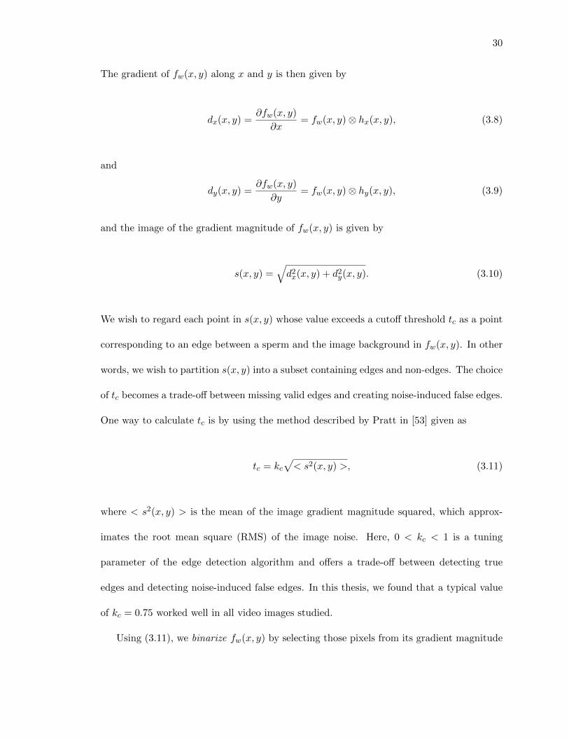
3.6 Details of the edge detection technique. (A) original image, (B) Wiener-filtering,(C) edge detection, (D) dilation, (E) close holes, (F) erode, (G) object labeling,(H) final detection results. . . . . . . . . . . . . . . . . . . . . . . . . . . . . . . 37
3.7 Original video frame A. . . . . . . . . . . . . . . . . . . . . . . . . . . . . . . . 38
3.8 Original video frame B. . . . . . . . . . . . . . . . . . . . . . . . . . . . . . . . 38
3.9 Morphologically enhanced detected edges in video frame A. . . . . . . . . . . . 39
3.10 Morphologically enhanced detected edges in video frame B. . . . . . . . . . . . 39
3.11 Output of Otsu’s intensity thresholding for video frame A. . . . . . . . . . . . . 40
3.12 Output of Otsu’s intensity thresholding for video frame B. . . . . . . . . . . . . 40
3.13 Result of multiplying the images in Figures 3.9 and 3.11. . . . . . . . . . . . . 41
3.14 Result of multiplying the images in Figures 3.10 and 3.12 . . . . . . . . . . . . 41
3.15 Final segmentation results for video frame A. . . . . . . . . . . . . . . . . . . . 42
3.16 Final segmentation results for video frame B. . . . . . . . . . . . . . . . . . . . 42
4.1 Steady-state DWNA ↵-� filter gains and normalized residual error vs trackingindex ⇤. . . . . . . . . . . . . . . . . . . . . . . . . . . . . . . . . . . . . . . . . 52

viii
4.2 Circular sperm trajectory. . . . . . . . . . . . . . . . . . . . . . . . . . . . . . . 56
4.3 Meandering sperm trajectory. . . . . . . . . . . . . . . . . . . . . . . . . . . . . 56
4.4 Average normalized innovations squared (NIS) vs time for 100 Monte Carlo runs. 57
4.5 True position, estimated position and validation gate for a simulated sperm. . . 57
4.6 Measurement-to-track association conflicts. . . . . . . . . . . . . . . . . . . . . 61
4.7 Number of feasible joint association events for m = n = 1 to 10. . . . . . . . . . 64
4.8 Example: five targets and five measurements in conflict. . . . . . . . . . . . . . 65
5.1 Number of sperm counted at ⇥200 magnification in field 1. . . . . . . . . . . . 78
5.2 Number of sperm counted at ⇥200 magnification in field 2. . . . . . . . . . . . 78
5.3 Illustration of dynamic sperm swimming parameters. . . . . . . . . . . . . . . . 80
6.1 Four examples of imperfect tracking. . . . . . . . . . . . . . . . . . . . . . . . . 83
6.2 Scenario A using PDAF: ground truth and estimated tracks. . . . . . . . . . . 87
6.3 Scenario A using PDAF: mean OSPA distance. . . . . . . . . . . . . . . . . . . 87
6.4 Scenario A using JPDAF: ground truth and estimated tracks. . . . . . . . . . . 88
6.5 Scenario A using JPDAF: mean OSPA distance. . . . . . . . . . . . . . . . . . 88
6.6 Scenario A using ENN-JPDAF: ground truth and estimated tracks. . . . . . . . 89
6.7 Scenario A using ENN-JPDAF: mean OSPA distance. . . . . . . . . . . . . . . 89
6.8 Scenario B using PDAF: ground truth and estimated tracks. . . . . . . . . . . 91
6.9 Scenario B using PDAF: mean OSPA distance. . . . . . . . . . . . . . . . . . . 91
6.10 Scenario B using JPDAF: ground truth and estimated tracks. . . . . . . . . . . 92
6.11 Scenario B using JPDAF: mean OSPA distance. . . . . . . . . . . . . . . . . . 92
6.12 Scenario B using ENN-JPDAF: ground truth and estimated tracks. . . . . . . . 93
6.13 Scenario B using ENN-JPDAF: mean OSPA distance. . . . . . . . . . . . . . . 93
6.14 Scenario C using PDAF: ground truth and estimated tracks. . . . . . . . . . . 95

ix
6.15 Scenario C using JPDAF: mean OSPA distance. . . . . . . . . . . . . . . . . . 95
6.16 Scenario C using JPDAF: ground truth and estimated tracks. . . . . . . . . . . 96
6.17 Scenario C using JPDAF: mean OSPA distance. . . . . . . . . . . . . . . . . . 96
6.18 Scenario C using ENN-JPDAF: ground truth and estimated tracks. . . . . . . . 97
6.19 Scenario C using ENN-JPDAF: mean OSPA distance. . . . . . . . . . . . . . . 97
6.20 Sperm swimming trajectory (black), instantaneous velocity (dashed line) andswimming direction angle . . . . . . . . . . . . . . . . . . . . . . . . . . . . . . 99
6.21 Simulated sperm trajectories at 1/30-sec intervals with and without head wob-bling using directional persistence times ⌧
p
= 0.1 sec, 0.01 sec, and 0.001 sec. . 100
6.22 Simulated 20⇥ 106/mL concentration: ground truth track history. . . . . . . . 103
6.23 Simulated 20⇥ 106/mL concentration using PDAF: mean OSPA distance. . . . 103
6.24 Simulated 20⇥ 106/mL concentration using JPDAF: mean OSPA distance. . . 104
6.25 Simulated 20⇥ 106/mL concentration using ENN-JPDAF: mean OSPA distance. 104
6.26 Simulated 40⇥ 106/mL concentration using PDAF: track history. . . . . . . . . 105
6.27 Simulated 40⇥ 106/mL concentration using PDAF: mean OSPA distance. . . . 105
6.28 Simulated 40⇥ 106/mL concentration using JPDAF: mean OSPA distance. . . 106
6.29 Simulated 40⇥ 106/mL concentration using ENN-JPDAF: mean OSPA distance. 106
6.30 Simulated 60⇥ 106/mL concentration: ground truth track history. . . . . . . . 107
6.31 Simulated 60⇥ 106/mL concentration using PDAF: mean OSPA distance. . . . 107
6.32 Simulated 60⇥ 106/mL concentration using JPDAF: mean OSPA distance. . . 108
6.33 Simulated 60⇥ 106/mL concentration using ENN-JPDAF: mean OSPA distance. 108
6.34 Percentage error in mean motility parameter measurements. . . . . . . . . . . . 110
7.1 Sample preparation. . . . . . . . . . . . . . . . . . . . . . . . . . . . . . . . . . 112
7.2 Five patients: sperm concentration (un-washed semen). . . . . . . . . . . . . . 117
7.3 Five patients: sperm concentration (washed semen). . . . . . . . . . . . . . . . 117

x
7.4 Five patients: percent motility (un-washed semen). . . . . . . . . . . . . . . . . 118
7.5 Five patients: percent motility (washed semen). . . . . . . . . . . . . . . . . . . 118
7.6 Five patients: percent forward progression (un-washed semen). . . . . . . . . . 119
7.7 Five patients: percent forward progression (washed semen). . . . . . . . . . . . 119
7.8 Patient No. 449, snapshot of multi-target tracking for chamber W1. . . . . . . 121
7.9 Patient No. 449, 30 sec track histories for fields A, B, and C. . . . . . . . . . . 122
7.10 Patient No. 449, VCL and VSL measurements for fields A, B, and C. . . . . . 123
7.11 Patient No. 449, LIN and ALH measurements for fields A, B, and C. . . . . . . 124
7.12 Patient No. 449, VCL measurements for fields A, B, and C. . . . . . . . . . . . 125
7.13 Patient No. 449, VSL measurements for fields A, B, and C. . . . . . . . . . . . 125
7.14 Patient No. 449, LIN measurements for fields A, B, and C. . . . . . . . . . . . 126
7.15 Patient No. 449, ALH measurements for fields A, B, and C. . . . . . . . . . . . 126
7.16 Patient No. 451, snapshot of multi-target tracking for chamber W1. . . . . . . 127
7.17 Patient No. 451, 30 sec track histories for fields A, B, and C. . . . . . . . . . . 128
7.18 Patient No. 451, VCL and VSL measurements for fields A, B, and C. . . . . . 129
7.19 Patient No. 451, LIN and ALH measurements for fields A, B, and C. . . . . . . 130
7.20 Patient No. 451, VCL measurements for fields A, B, and C. . . . . . . . . . . . 131
7.21 Patient No. 451, VSL measurements for fields A, B, and C. . . . . . . . . . . . 131
7.22 Patient No. 451, LIN measurements for fields A, B, and C. . . . . . . . . . . . 132
7.23 Patient No. 451, ALH measurements for fields A, B, and C. . . . . . . . . . . . 132
7.24 Patient No. 495, snapshot of multi-target tracking for chamber W1. . . . . . . 133
7.25 Patient No. 495, 30 sec track histories for fields A, B, and C. . . . . . . . . . . 134
7.26 Patient No. 495, VCL and VSL measurements for fields A, B, and C. . . . . . 135
7.27 Patient No. 495, LIN and ALH measurements for fields A, B, and C. . . . . . . 136

xi
7.28 Patient No. 495, VCL measurements for fields A, B, and C. . . . . . . . . . . . 137
7.29 Patient No. 495, VSL measurements for fields A, B, and C. . . . . . . . . . . . 137
7.30 Patient No. 495, LIN measurements for fields A, B, and C. . . . . . . . . . . . 138
7.31 Patient No. 495, LIN measurements for fields A, B, and C. . . . . . . . . . . . 138
7.32 Patient No. 544, snapshot of multi-target tracking for chamber W1. . . . . . . 139
7.33 Patient No. 495, 30 sec track histories for fields A, B, and C. . . . . . . . . . . 140
7.34 Patient No. 544, VCL and VSL measurements for fields A, B, and C. . . . . . 141
7.35 Patient No. 544, VCL and VSL measurements for fields A, B, and C. . . . . . 142
7.36 Patient No. 544, VCL measurements for fields A, B, and C. . . . . . . . . . . . 143
7.37 Patient No. 544, VSL measurements for fields A, B, and C. . . . . . . . . . . . 143
7.38 Patient No. 544, LIN measurements for fields A, B, and C. . . . . . . . . . . . 144
7.39 Patient No. 544, ALH measurements for fields A, B, and C. . . . . . . . . . . . 144
7.40 Patient No. 562, snapshot of multi-target tracking for chamber W1. . . . . . . 145
7.41 Patient No. 562, 30 sec track histories for fields A, B, and C. . . . . . . . . . . 146
7.42 Patient No. 562, VCL and VSL measurements for fields A, B, and C. . . . . . 147
7.43 Patient No. 562, LIN and ALH measurements for fields A, B, and C. . . . . . . 148
7.44 Patient No. 562, VCL measurements for fields A, B, and C. . . . . . . . . . . . 149
7.45 Patient No. 562, VSL measurements for fields A, B, and C. . . . . . . . . . . . 149
7.46 Patient No. 562, LIN measurements for fields A, B, and C. . . . . . . . . . . . 150
7.47 Patient No. 562, ALH measurements for fields A, B, and C. . . . . . . . . . . . 150

xii
List of Symbols and Nomenclature
2 element of
� Minkowski addition
Minkowski substraction
⌦ two-dimensional discrete convolution operator
Cov(.) covariance operator
E(.) expectation operator
Var(.) variance operator
(.)c complement (of an image) operator
(.)T matrix transpose operator
d.e ceiling operator, i.e., round up to nearest integer
N [µ;Px
] Gaussian distributed random variable with mean µ and covariance Px
In⇥n
n⇥ n identity matrix
(k|k � 1) denotes quantity at time k given a measurement at time k � 1
(k|k) denotes quantity at time k given a measurement at time k
xt
(k) 4⇥ 1 state vector for target t at time k
zt
(k) 2⇥ 1 position measurement vector for target t at time k
wt
(k) 2⇥ 1 process noise vector for target t at time k
nt
(k) 2⇥ 1 position measurement noise vector for target t at time k
W (k) 2⇥ 2 covariance matrix of wt
(k) at time k
N(k) 2⇥ 2 measurement noise covariance matrix at time k
�2w
process noise variance (assumed equal in x and y directions)
�2n
sensor measurement noise variance (assumed equal in x and y directions)
T time between sensor measurements (sec)
F 4⇥ 4 system dynamics matrix
G 4⇥ 2 system input matrix
H 2⇥ 4 measurement matrix

xiii
zj
(k) 2⇥ 1 j–th position measurement received at time k
tj
index of the target that measurement j is associated with
xt
(k|k) 4⇥ 1 estimated state of target t at time k given a measurement at time k
xt
(k|k � 1) 4⇥ 1 predicted state of target t at time k given a measurement at time k� 1
Pt
(k|k) 4⇥ 4 state estimation error covariance matrix for target t at time k given ameasurement at time k
Pt
(k|k � 1) 4⇥ 4 predicted state estimation error covariance matrix for target t at timek given a measurement at time k � 1
Q(k) 4⇥ 4 process noise covariance matrix at time k
zt
(k|k � 1) 2⇥1 predicted position measurement for target t at time k given a measure-ment at time k � 1
⌫jt
(k) 2⇥ 1 residual or innovation vector for target t using measurement j
St
(k) 2⇥ 2 residual or innovation covariance matrix for target t at time k
Kt
(k) 4⇥ 2 Kalman filter gain matrix for target t at time k
↵,� scalar steady-state Kalman filter position and velocity gains (dimensionless)
⇤ target tracking index (dimensionless)
PG
probability that the track gate would contain a measurement if the targetwas detected
� position gate threshold (dimensionless)
Vmax
velocity gate threshold (µm/sec)
Z(k) the set of all measurements received at time k
Zk the set of all measurements received up to and including time k
P t
D
probability of detection of target t
Ljt
(k) likelihood ratio that measurement zj
(k) originated from target t rather thanfrom clutter at time k
�jt
(k) the marginal probability that measurement zj
(k) is associated to target t attime k
�0t
(k) the marginal probability that none of the measurements is associated totarget t at time k
� the expected number of measurements due to clutter per unit area of thesurveillance space per scan of data (assumed to be Poisson distributed withmean �)

xiv
�n
the expected number of new targets per unit area of the surveillance spaceper scan of data (assumed to be Poisson distributed with mean �
n
)
⌫t
(k) 2⇥ 1 probability-weighted combined residual vector
P c
t
(k|k) 4⇥4 measurement-updated state estimation error covariance matrix for tar-get t at time k that would be obtained in the absence of measurement originuncertainty
Pt
(k) 4⇥ 4 matrix of the spread of the innovations for target t at time k
✓(k) joint association event at time k
⌧j
(✓) binary measurement association indicator; ⌧j
(✓) = 1 if measurement j isassociated with any target in event ✓ (zero otherwise)
�t
(✓) binary target detection indicator; �t
(✓) = 1 if target t is associated with anymeasurement in event ✓ (zero otherwise)
!jt
(✓, k) indicates if measurement j is associated with target t in joint associationevent ✓(k)
P ✓(k)|Zk probability of the joint association event ✓(k) given all of the measurementsup to time k
`t
(k) track score of target t equal to the cumulative negative log of the likelihoodratio L
jt
(k) for target t at time k
�`t
(k) track score increment for target t at time k
PDT
probability of deleting a true track
PCF
probability of confirming a false track
Xk
set of q labeled ground truth target track positions at time k
Yk
set of r labeled estimated target track positions at time k
do
(Xk
,Yk
) optimal subpattern assignment distance between Xk
and Yk
k
xk,i
the position of ground truth track i with label lxi
, i = 1 . . . q
yk,j
the position of ground truth track j with label lxj
, j = 1 . . . r
d(x,y) localization base distance
p optimal subpattern assignment order parameter (p > 0)
c localization error penalty (c > 0)
⇠ labeling error penalty (0 ⇠ c)
sperm swimming direction angle (radians)
V simulated sperm swimming speed (µm/sec)

xv
⌧p
directional persistence time of simulated sperm swimming angle (sec)
ALH amplitude of lateral head displacement
BCF beat cross frequency
CASA computer-assisted semen analysis
DWNA discrete white noise acceleration
ENN-JPDAF exact nearest-neighbor JPDAF
FOV field of view
HA hyaluronic acid
ICSI intracytoplasmic sperm injection
IUI intrauterine insemination
IVF in-vitro fertilization
JPDAF joint probabilistic data association filter
LIN swimming path linearity
LOA limits of agreement
MHI motion history image
MHT multiple hypothesis tracker
OSPA optimal subpattern assignment
PDAF probabilistic data association filter
SNR signal-to-noise ratio
VCL curvilinear velocity
VSL straight-line velocity
xvi
AbstractRobust Automatic Multi-Sperm Tracking in Time-Lapse Images
Leonardo F. UrbanoMoshe Kam, PhD
Human sperm cell counting, tracking and motility analysis is of significant interest to bi-
ologists studying sperm function and to medical practitioners evaluating male infertility.
Today, the prevailing method for analyzing sperm at fertility clinics and research laborato-
ries is laborious and subjective. Namely, the number and quality of sperm are often visually
appraised by technicians using a microscope. Although total sperm count and sperm con-
centration can be reasonably estimated when standard protocols are applied, they have
little diagnostic value except in identifying pathologically extreme abnormalities. More dy-
namic sperm swimming parameters such as curvilinear velocity (VCL), straight-line velocity
(VSL), linearity of forward progression (LIN) and amplitude of lateral head displacement
(ALH) are increasingly believed to have clinical significance in predicting infertility but
are impossible for a human observer to visually discern. Expensive computer-assisted se-
men analysis (CASA) instruments are also sometimes used but are severely encumbered
by crude ad-hoc tracking algorithms which cannot track sperm in close proximity or whose
paths intersect and are typically limited to analyzing video clips of 1 sec duration.
In this thesis, we present a robust automatic multi-sperm tracking algorithm that can
measure dynamic sperm motility parameters over time in pre-recorded time-lapse images.
This e↵ort is informed by progress in signal processing and target tracking technologies over
the last three decades. Multi-target tracking algorithms originally developed for radar, sonar
and video processing have addressed similar problems in other domains. In this thesis, we

xvii
demonstrate that their methodologies can be used for sperm tracking and motility analysis.
To resolve sperm measurement-to-track association conflicts, we applied and evaluated three
multi-target tracking algorithms: the probabilistic data association filter (PDAF), the joint
probabilistic data association filter (JPDAF) and the exact nearest neighbor extension to the
JPDAF (ENN-JPDAF). We validated the accuracy of our tracking and motility analysis by
using simulated sperm trajectories whose ground truth tracks were perfectly known. Using
samples collected from five patients at a fertility clinic, we demonstrated automatic sperm
detection and tracking even during challenging multi-sperm collision events.
Combined analysis, testing and simulation support the use of probabilistic data as-
sociation techniques robust automatic multi-sperm tracking. This method could provide
fertility specialists with new data visualizations and interpretations previously impossible
with existing laboratory protocols.

1
Chapter 1: Introduction
Sperm cell counting, tracking and classification is of significant interest to biologists study-
ing sperm function and to medical practitioners evaluating and treating male reproductive
pathology [1, 2]. For example, human sperm are routinely examined at fertility clinics
around the world as the first step in identifying the cause of a couples’ suspected infertility
[3]. If a couple elects to use assistive reproductive technology (ART), then partner or donor
semen is analyzed to select candidate sperm for in-vitro fertilization (IVF), intracytoplas-
mic sperm injection (ICSI), or intra-uterine insemination (IUI) [4]. Sperm analysis can also
indicate the presence of toxins or the onset of other diseases [5]. Sperm analysis is increas-
ingly applied by veterinary practitioners for industrial animal husbandry and commercial
stud farming.
Today, the prevailing method for analyzing human sperm at fertility clinics is both la-
borious and subjective [6, 7]. Namely, the number and quality of sperm are often visually
appraised by technicians by examining a sample of patient sperm using a microscope. In
order to minimize the variability of test results from laboratory to laboratory, standard
protocols have been developed to make routine sperm analysis more objective and repro-
ducible, the most notable of which is the World Health Organization (WHO) Manual for
the Examination and Processing of Human Semen [1]. Using such protocols, it is possible
for a trained technician to estimate with some accuracy the total concentration of sperm
in an ejaculate and the percentage of sperm exhibiting progressive motility, both of which
are believed to have clinical significance in predicting infertility. Despite the availability of
such protocols, di↵erences between laboratories persist [8, 9].

2
Attempts to make sperm analysis more objective began in the mid-1980s with the intro-
duction of computer-assisted semen analysis (CASA) systems [10, 11]. Such CASA systems
use computers to digitally capture a sequence of video frames from a microscope and apply
digital image processing algorithms to automatically detect and count sperm cells. In addi-
tion, CASA systems can reconstruct the swimming paths of sperm over several video frames
and thus enables the measurement of dynamic swimming parameters including curvilinear
velocity (VCL), straight-line velocity (VSL), linearity of forward progression (LIN), and
amplitude of lateral head displacement (ALH) – all of which are impossible for a human
observer to visually discern.
Unfortunately, today’s CASA systems remain prohibitively expensive and require sub-
stantial user intervention to operate [8]. This is in part because nearly all CASA systems
employ crude ad-hoc tracking algorithms that are unable to reconstruct the paths of sperm
swimming in close proximity or during near-misses and collisions [12, 2, 10]. This limitation
restricts the usefulness of CASA to the analysis of low-density sperm samples or high-density
sperm samples that have been diluted with a patients own seminal plasma (which may not
always be possible with available clinical material) [2]. As a result, CASA instruments are
estimated to be used in < 2% of laboratories processing human semen and < 20% of major
andrology laboratories in the United States [11]. Over the last 30 years, CASA has failed
to replace manual sperm analysis, depriving biologists and medical specialists of a practical
tool to enhance our understanding of sperm function.
1.1 Thesis Overview
In this thesis, our primary objective is to develop a fully-automated, robust, multi-sperm
tracking algorithm capable of accurately measuring sperm motility parameters from time-

3
lapse images with minimal operator intervention. This e↵ort is informed by progress in
signal processing and target tracking technologies over the last three decades. Multi-target
tracking algorithms originally developed for radar and sonar applications and video pro-
cessing have addressed similar problems in other domains. In this thesis, we demonstrate
that their methodologies can be used for sperm tracking and analysis.
This thesis is organized into eight chapters that discuss the problem of automatic sperm
detection, tracking and motility analysis. Chapters 2 through 8 provide the following infor-
mation.
Chapter 2. Background and Literature Review. This chapter discusses the develop-
ment and physiology of human sperm cells, describes a typical semen analysis, and reviews
the capabilities and limitations of existing CASA systems. Several multi-target tracking
algorithms originally developed for radar, sonar and video processing applications are then
briefly described. Lastly, previous works in the area of multi-sperm tracking and analysis
that influenced this thesis are discussed.
Chapter 3. Sperm Cell Imaging and Pixel Segmentation. This chapter describes
the process of imaging human sperm samples using a digital microscope including the neces-
sary video pre-processing required before sperm segmentation can be performed on recorded
video image frames. Next, the four common techniques for cell segmentation are briefly
described: intensity thresholding, feature detection, morphological filtering and region ac-
cumulation. The combined approach used in this thesis to segment sperm cells – namely,
an intensity thresholding operation combined with a feature detection and morphological
filtering operation – is described in detail and example segmentation results from our track-
4
ing experiments are presented.
Chapter 4. Multi-Sperm Tracking. This chapter presents a Kalman filter with mea-
surement gating applied to a discrete white noise acceleration (DWNA) target model
for tracking human sperm cells and discusses selection of filter parameters. The multi-
measurement and multi-target extensions of this Kalman filter – namely, the probabilistic
data association filter (PDAF) and the joint probabilistic data association filter (JPDAF)
– are presented and their relative strengths and weaknesses discussed. Special attention is
given to the computationally expensive process of enumerating every feasible joint associ-
ation event required by the JPDAF. A simpler approach that rapidly identifies only the
most highly probable joint events using Murty’s method for finding the M -best ranked as-
signments is then demonstrated. Fitzgerald’s exact nearest neighbor (ENN)-JPDAF which
avoids track coalescence is then presented. Finally, multi-target tracking implementation
issues such as track management (i.e., initiation, continuation and deletion) and track clus-
tering are discussed.
Chapter 5. Sperm Counting and Motility Analysis. This chapter describes the stan-
dard methodology for calculating sperm concentration, percent motility and percentage of
sperm exhibiting forward progression. In addition, formulas for the calculation of VCL,
VSL, LIN and ALH using track data produced by our algorithm is then discussed.
Chapter 6. Tracking Results Using Simulations. This chapter presents results ob-
tained by applying the PDAF, JPDAF and ENN-JPDAF algorithm to three simple multi-
target scenarios. To objectively compare algorithms, Ristic’s extension of Schuchmachers
5
optimal subpattern assignment (OSPA) distance to labeled tracks is presented and calcu-
lated using the set of perfectly known ground truth tracks and the set of estimated tracks
produced by each algorithm. Next, the three algorithms are applied to realistic simulated
scenes of swimming sperm at three di↵erent concentrations and their performances com-
pared using the OSPA distance averaged over Monte Carlo replications of each scene. Fi-
nally, we compare motility measurements collected by each algorithm in each of three scenes.
Chapter 7. Tracking Results Using Time-Lapse Images. This chapter presents
the tracking results and motility parameter measurements obtained by applying the ENN-
JPDAF algorithm to time-lapse images of sperm from five human subjects collected at a
fertility clinic.
Chapter 8. Concluding Remarks. This chapter provides concluding remarks about
the thesis, summarizes the accomplishments and contributions and identifies areas of future
study.

6
Chapter 2: Background and Literature Review
In this chapter, we briefly describe the development and physiology of human spermatozoa,
give an overview of the standard semen analysis, and review previous work in the area of
multi-target tracking including automatic sperm tracking. This work includes CASA in-
strumentation, biomedical image processing and radar and sonar tracking and surveillance
technologies. Lastly, we identify how the reviewed work was extended to fit the unique
requirements of our application.
2.1 Development and Physiology of Human Spermatozoa
Sperm are produced in the seminiferous tubules of the adult male testes in a complex
process called spermatogenesis that takes place over a period of 60–70 days [2]. During
spermatogenesis, a tiny germ cell called a spermatogonia splits into multiple daughter cells,
each of which is capable of becoming a spermatocyte and eventually a spermatid. The
maturation of a spermatid into a recognizable testicular sperm occurs during the process
of spermiogenesis. Mature sperm are then transported and stored in the epididymis – a
narrow tightly-coiled tube nearly six to seven meters long [13] – until ejaculation. Over
the normal course of spermatogenesis in a healthy adult male, approximately 1,200 sperm
achieve maturation with every heartbeat, or approximately 120 million sperm per day [14].
The number and concentration of sperm exhibits wide intra-individual variation over time
[1].
The typical human sperm has three major and clearly discernible parts: a head, a

7
Figure 2.1: Diagram of a human spermatozoa.
midpiece and a tail (see Figure 2.1). The head is approximately 3–5 µm long and 2–3 µm
wide and is comprised of a nucleus which contains genetic material and a cap-like acrosome
which contains digestive enzymes necessary for penetration of the sperm into the female
oocyte. The thickened midpiece between the head and tail is the engine of the sperm and
is approximately 7–8 µm long and 1 µm wide and comprised of spiral-like mitochondria.
Finally, the whip-like tail or flagella is about 50 µm long [1, 2].
It is interesting to note that contrary to popular belief, nearly all testicular sperm
are immotile and acquire motility only after ejaculation when they are mixed with the
secretions of the accessory glands of the vas deferens, seminal vesicles and the prostate [2].
Immediately after ejaculation, semen is a thick coagulated mass comprised of sperm and
gelatinous bodies. Sperm cells themselves only account for 1–5% of the total volume of
ejaculate. Over a period of 15–30 minutes at room temperature, semen attains a watery
consistency due to a process known as liquefaction after which sperm motility is markedly
increased. The most typical swimming pattern (> 90%) is the forward-progressive but
meandering path characterized by distinct sinusoidal head motion, while the rarest (< 3%)
is the so-called hyperactivated or “star-spin” swimming pattern characterized by extremely
8
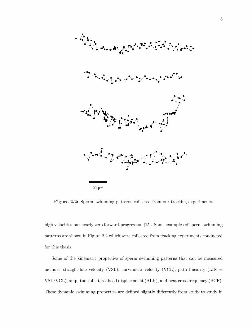
Figure 2.2: Sperm swimming patterns collected from our tracking experiments.
high velocities but nearly zero forward-progression [15]. Some examples of sperm swimming
patterns are shown in Figure 2.2 which were collected from tracking experiments conducted
for this thesis.
Some of the kinematic properties of sperm swimming patterns that can be measured
include: straight-line velocity (VSL), curvilinear velocity (VCL), path linearity (LIN =
VSL/VCL), amplitude of lateral head displacement (ALH), and beat cross frequency (BCF).
These dynamic swimming properties are defined slightly di↵erently from study to study in
9
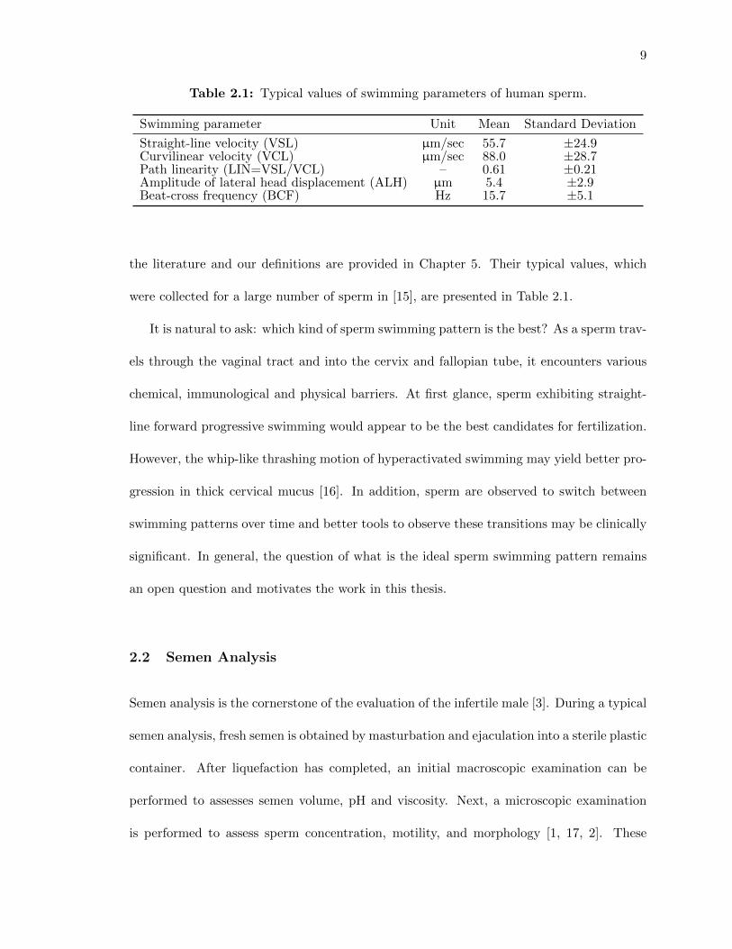
Table 2.1: Typical values of swimming parameters of human sperm.
Swimming parameter Unit Mean Standard Deviation
Straight-line velocity (VSL) µm/sec 55.7 ±24.9Curvilinear velocity (VCL) µm/sec 88.0 ±28.7Path linearity (LIN=VSL/VCL) – 0.61 ±0.21Amplitude of lateral head displacement (ALH) µm 5.4 ±2.9Beat-cross frequency (BCF) Hz 15.7 ±5.1
the literature and our definitions are provided in Chapter 5. Their typical values, which
were collected for a large number of sperm in [15], are presented in Table 2.1.
It is natural to ask: which kind of sperm swimming pattern is the best? As a sperm trav-
els through the vaginal tract and into the cervix and fallopian tube, it encounters various
chemical, immunological and physical barriers. At first glance, sperm exhibiting straight-
line forward progressive swimming would appear to be the best candidates for fertilization.
However, the whip-like thrashing motion of hyperactivated swimming may yield better pro-
gression in thick cervical mucus [16]. In addition, sperm are observed to switch between
swimming patterns over time and better tools to observe these transitions may be clinically
significant. In general, the question of what is the ideal sperm swimming pattern remains
an open question and motivates the work in this thesis.
2.2 Semen Analysis
Semen analysis is the cornerstone of the evaluation of the infertile male [3]. During a typical
semen analysis, fresh semen is obtained by masturbation and ejaculation into a sterile plastic
container. After liquefaction has completed, an initial macroscopic examination can be
performed to assesses semen volume, pH and viscosity. Next, a microscopic examination
is performed to assess sperm concentration, motility, and morphology [1, 17, 2]. These

10
Table 2.2: Lower limits of the accepted reference values for semen analysis.
On at least two occasions Reference value
Ejaculate volume 1.5 mLSemen pH 7.2Sperm concentration 15⇥106 sperm/mLTotal sperm number 39⇥106 sperm/ejaculatePercent motility 40%Forward progression 32%Normal morphology 4% normalSperm agglutination absentViscosity 2 cm thread post-liquefaction
measured semen parameters are then compared against the lower limits of their accepted
reference values, the most recent of which are reproduced from [1] in Table 2.2. In practice,
these lower reference limits are intended only to help classify men as fertile or sub-fertile
and to identify abnormalities and are not intended to reflect normal sperm parameters of
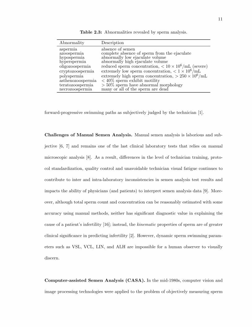
the general population [3]. A list of some of the many abnormalities that may be identified
by a semen analysis is provided in Table 2.3 (taken from [2]).
The primary tool of semen analysis is the laboratory microscope. Today, a vast major-
ity of semen analysis is done manually by technicians who visually appraise semen quality
in accordance with standard protocols [1]. Sperm concentration is typically measured by
manually identifying and counting sperm using a microscope ocular lens embedded with a
10⇥10 counting grid, or other specialized counting chambers may be used. The number
of sperm counted within the grid pattern is then multiplied by a scale factor (di↵erent for
each microscope and obtained by calibration) that relates the grid area to a fractional vol-
ume and ultimately to concentration expressed as millions of sperm per mL [1, 18]. The
percentage of motile sperm is typically calculated as the percentage of counted sperm ex-
hibiting any motion whatsoever (progressive or non-progressive). The percentage of motile
sperm exhibiting forward progression is typically as the percentage of counted sperm having
11
Table 2.3: Abnormalities revealed by sperm analysis.
Abnormality Description
aspermia absence of semenazoospermia complete absence of sperm from the ejaculatehypospermia abnormally low ejaculate volumehyperspermia abnormally high ejaculate volumeoligozoospermia reduced sperm concentration, < 10⇥ 106/mL (severe)cryptozoospermia extremely low sperm concentration, < 1⇥ 106/mLpolyspermia extremely high sperm concentration, > 250⇥ 106/mLasthenozoospermia < 40% sperm exhibit motilityteratozoospermia > 50% sperm have abnormal morphologynecrozoospermia many or all of the sperm are dead
forward-progressive swimming paths as subjectively judged by the technician [1].
Challenges of Manual Semen Analysis. Manual semen analysis is laborious and sub-
jective [6, 7] and remains one of the last clinical laboratory tests that relies on manual
microscopic analysis [8]. As a result, di↵erences in the level of technician training, proto-
col standardization, quality control and unavoidable technician visual fatigue continues to
contribute to inter and intra-laboratory inconsistencies in semen analysis test results and
impacts the ability of physicians (and patients) to interpret semen analysis data [9]. More-
over, although total sperm count and concentration can be reasonably estimated with some
accuracy using manual methods, neither has significant diagnostic value in explaining the
cause of a patient’s infertility [16]; instead, the kinematic properties of sperm are of greater
clinical significance in predicting infertility [2]. However, dynamic sperm swimming param-
eters such as VSL, VCL, LIN, and ALH are impossible for a human observer to visually
discern.
Computer-assisted Semen Analysis (CASA). In the mid-1980s, computer vision and
image processing technologies were applied to the problem of objectively measuring sperm

12
swimming parameters. This technique, referred to as computer-assisted semen analysis
(CASA), uses digital microscopes and image processing software to help automate the pro-
cess of sperm detection, tracking and classification and provides researchers and clinicians
with an objective and quantitative assessment of sperm swimming dynamics. A detailed
review of the historical development and commercialization of CASA instruments is given
in [11]. Nearly all CASA systems operate in two basic steps: (1) identification of sperm in
recorded video frames, and (2) reconstruction of the sperm swimming paths over a sequence
of video frames. After the swimming paths have been reconstructed, the motility param-
eters of individual sperm can be calculated and statistically summarized to characterize a
sample population.
Precise details of the algorithms employed by commercial CASA systems are scarce, but
detailed evaluations of such commercial systems and the available literature on the principles
of the CASA methodology are abundant [7, 10, 19, 20, 21, 22, 23, 24, 25, 26, 27, 28, 29].
From these reports, it is apparent that many CASA systems employ similar (and crude) ad-
hoc tracking algorithms that are unable to reliably reconstruct the paths of sperm swimming
in close proximity or during near-misses and collisions [12, 2, 10].
The basic methodology used by most CASA systems to reconstruct the swimming paths
of sperm is essentially to “connect-the-dots” and is illustrated in Figure 2.3A. Specifically, a
circle is drawn around the position of a sperm detected in the first video frame. The radius
of the circle is equal to the maximum displacement a sperm is expected to travel between
video frames. This maximum displacement (or maximum velocity) is often a user-defined
parameter, which may require user input or tuning for each sample. In the next frame, the
sperm has moved to a new position, but is still inside the first circle, and so a line is drawn
connecting the previous and new position. The circle is then re-centered at the new sperm

13
Figure 2.3: Typical ad-hoc tracking methodology used by many CASA systems.
position and the process is repeated until the entire sperm path is reconstructed.
In many CASA systems, if more than one sperm is detected within a circle on a given
frame, as depicted in Figure 2.3B, there is an ambiguity about which sperm should be used
to extend the track. The most common action taken by CASA instruments in this situation
is to terminate the paths and exclude the sperm in question from analysis [2, 12]. This
tends to bias the analysis of the sample toward the slower cells, since faster sperm have a
higher probability of being involved in such near-misses and of thus being excluded from
analysis. In other systems, the sperm closest to the center of the circle is used continue the
path reconstruction (i.e., nearest neighbor). This can result in the incorrect joining of two
distinctly di↵erent sperm paths (a track swap) which can cause errors in the calculation of
sperm motility parameters [10].
The inability for CASA instruments to reliably reconstruct the swimming paths of sperm
in close proximity or whose paths intersect restricts their usefulness to the analysis of low-
density sperm samples [2]. Nearly all of these crude tracking algorithms are appearance-

14
based (i.e., model-free) in which a-priori mathematical models of sperm kinematics are
seldom used in the tracking process. Instead, knowledge of sperm motion (e.g., maximum
speed) is applied in a heuristic or ad-hoc manner, usually in the form of a list of various tun-
ing knobs that the user must carefully adjust. Changing the settings of a CASA instrument
can yield vastly di↵erent measurements for the same sample [30].
Despite its advantages over manual methods, it is estimated that CASA is used in < 2%
of laboratories evaluating human semen and < 20% of major andrology laboratories in the
United States [11]. The limited use of CASA is primarily due to the prohibitively high cost
of associated equipment and technician training [8]. Training is necessary because CASA
instruments are sensitive to their parameter settings, which require adjustment for process-
ing di↵erent kinds of samples. In fact, the degree of necessary human intervention required
to obtain useful measurements with CASA systems can be as time-consuming as manual
methods, and so the benefits of automation are not fully realized for the costs incurred [12].
2.3 Multi-target Tracking
The problem of simultaneously tracking multiple targets has been studied extensively by the
radar and sonar tracking and surveillance community for decades. The number of papers
and texts dealing with this subject number in the thousands and so a complete review
cannot be presented here, although we refer the reader to some important classical texts on
the subject [31, 32, 33]. In recent years, interest in biomedical image and cell tracking has
exploded [34, 35, 36, 37].
When processing a scan of data from a radar, sonar or digital microscope sensor, mea-
surements may originate from targets of interest, from false detections due to random sensor
measurement noise (i.e., clutter), or from other nearby targets which may or may not al-
15
ready be in track. When studying cells using digital microscopy, a cell may swim in and
out of the focal plane and fail to be detected only to return at a later time at a di↵erent
spatial position. Furthermore, depending on the microscope sensor resolution, two or more
targets may be so close together that only a single merged measurement is produced.
A central problem in multi-target tracking is the so called data association problem. Data
association answers the question: “to which target does this measurement correspond?”
and is sometimes referred to as the motion correspondence problem. There are two basic
classes of data association techniques: deterministic and probabilistic. An example of a
deterministic data association technique is the simple nearest-neighbor scheme [32] whereby
the measurement closest to the predicted position of a target is used to update and extend its
track and all other measurements discarded. A more sophisticated technique is the so-called
global nearest-neighbor (GNN) scheme [33] in which a matrix of pairwise distances between
every track and measurement is formed and the optimal permutation of assignments of
measurements to tracks is found such that the sum of the distances of the assignments is
a minimum over all other possible assignment permutations. Such techniques work well in
a benign target environment, but can face di�culties in situations where the number of
real or false targets is large. Furthermore, since knowledge of the target dynamics are not
used, correct association when many targets and measurements are in close proximity can
be problematic.
On the other end of the spectrum are the probabilistic data association techniques.
A detailed review on the use of probabilistic methods for data association for tracking in
biomedical images is given by Rasmussen in [38]. These schemes employ a dynamical model
of target motion and a model of the measurement process in order to estimate the state of
a target using a sequence of measurements, usually in the form a Kalman filter. Among

16
these techniques, the so-called multi-hypothesis tracker (MHT) [39] is regarded as the most
accurate solution to the general multi-target tracking problem. In the MHT approach, the
states and state estimation error covariances provided by each target filter is used to identity
every feasible measurement-to-track association hypothesis over a certain time depth which
are used to calculate a set of association probabilities. The computational and memory
requirements of MHT-based methods, however, increase exponentially with the number of
objects tracked and with the total tracking duration. This makes MHT unattractive for
many time-critical applications.
A widely-used sub-optimal probabilistic data association scheme that has been imple-
mented in many real-world applications is the so-called probabilistic data association filter
(PDAF) [40] which considers only two possible measurement origin hypotheses: measure-
ments originate either from the target of interest or they originate from clutter. The PDAF
is very e↵ective for tracking single targets in clutter, but in a target-rich environment the
persistent presence of measurements from nearby targets can cause severe tracking degra-
dation. The natural multi-target extension of the PDAF is the joint probabilistic data
association filter (JPDAF) which considers the possibility that measurements could have
originated from targets already being tracked [41]. Similar to MHT, the JPDAF calcu-
lates every measurement-to-track association hypothesis jointly across all targets. Unlike
the MHT, only the latest scan of data is used (i.e., it is approximately the MHT with a
time-depth of one scan). In this sense, the JPDAF approximates the MHT at considerably
less computational cost but has performance comparable to that of the MHT [42].

17
2.4 Previous Work in Automatic Sperm Tracking
In this section, we discuss a number of previous works in automatic sperm and biomedical
particle tracking which influenced the work in this thesis.
In [43], Young describes a real-time ad-hoc sperm tracking system that di↵ers in a
number of ways from existing CASA systems and techniques. Namely, Young uses a pixel
grayscale detection threshold to discriminate sperm from background pixels, tracks each
sperm until a pre-specified number of points have been collected or until the sperm swims
out of the microscopic field-of-view, and outputs summary statistics for the motility mea-
surements collected for all of a pre-specified number of sperm. In addition, tracks are
automatically initiated and terminated as sperm enter and exit the microscopic field-of-
view, which relieves technicians from having to select multiple fields within a sample. This
has the advantage of also minimizing the potential e↵ect of technician bias when selecting
fields, as technicians tend to select fields containing a large number of sperm [1]. In contrast,
most CASA systems typically analyze only 5 to 30 frames (typically 1 second of video) and
do not initiate tracks on new sperm entering the microscopic field-of-view. Young also ob-
serves that although the motility parameters di↵er for individual sperm, the values for the
entire specimen become stable when a large number of sperm are traced over time, which
also reveal the temporal changes in sperm swimming patterns which cannot be observed by
typical CASA instruments.
In [44], Beresford-Smith discusses the application of radar tracking algorithms to the
problem of sperm tracking. Specifically, a Kalman filter and PDAF are presented wherein
the target state vector is augmented with the maximum pixel brightness of each sperm.
Using this technique, real-time single-sperm tracking is achieved, although no detailed re-
sults were presented or discussed. However, given the fact that PDAF performs poorly in

18
scenes with large numbers of real and false targets, it is unlikely that a PDAF-based multi-
sperm tracking algorithm is practical for clinical sperm analysis except for very low density
samples. We explore this hypothesis in Chapter 6 when we apply the PDAF to tracking
simulated sperm at di↵erent concentrations.
In [4], Liu discusses experiments using a Kalman filter to quantify the locomotive be-
havior of human sperm heads and tails. Sperm head tracking is done using a motion history
image (MHI)-based approach in which a sequence of video frames are blended to form a
smeared image of the path traced by moving sperm. A curve is fitted to each smear and
used to calculated VCL, VSL and LIN. To study sperm tails, an aliquot of sperm placed on
a dish coated with hyaluronic acid (HA) causes healthy mature sperm to bind to the dish as
though it were a female oocyte. Upon binding, sperm tails can be seen to flicker vigorously.
The sperm tails are detected by analyzing the pixels in a region near the sperm head in the
direction opposite the sperm motion, and the di↵erence in the position of sequential tail
detections in the flickering image is averaged and regarded as the tail beating amplitude.
It is hypothesized that those sperm whose tails beat most vigorously are prime “healthy”
candidates for IVF, ICSI and IUI. Liu’s paper thus demonstrates a novel application of
automatic sperm tracking in the area of sperm selection. A disadvantage of the MHI-based
approach is that it cannot detect or track immotile sperm or debris which can lead to errors
in the reconstructed paths of motile sperm.
In [45], Tomlinson discusses the application and validation of a novel CASA system that
employs a multi-target tracking algorithm. Specifically, Khan’s Markov chain Monte Carlo
(MCMC)-based tracking algorithm [46] is applied, which uses particle filters and a term to
account for potential “interaction” between multiple sperm in close proximity. A validation
experiment comparing the concentration and motility measurements of sperm samples using

19
the new CASA instrument to measurements obtained by “gold standard” manual analysis
performed by technicians shows good agreement. A combination of automatic image pro-
cessing and user intervention is used to detect sperm in recorded videos. Tracking is limited
to only 30 frames (1 second).
In [15, 47, 48], Su presents a lensfree on-chip holographic imaging platform capable of
tracking sperm in 3D over a large (4.2⇥4.2⇥5.8 cm) field-of-view. This new sensor enables
for the first time the observation of helical swimming patterns in 4–5% of human sperm
and allows for detecting changes in sperm swimming patterns over time. Specific details of
the tracking algorithm employed by this system are not presented, except for a reference
to Crocker’s technique [49] for tracking particles in videos of colloidal suspensions, which
is based loosely on a modified nearest-neighbor scheme. Although the technique is able to
track sperm in 3D, each analyzed track segment is typically only 10–20 seconds long and
only very low concentration samples (< 9⇥ 106/mL) are imaged. Furthermore, it requires
2.2 hours to process approximately 20 minutes of holographic video.
In [36], Chenouard describes an objective comparison of particle tracking methods.
Three main factors are identified as a↵ecting performance: dynamics (type of particle mo-
tion), density (number of particles within the field-of-view), and signal (relative to noise).
A set of simulated video sequences exhibiting a range of particle dynamics, densities and
SNR are provided to participants in an open competition between members of the tracking
community in 2012. Several multi-target tracking techniques are evaluated including a vari-
ety of deterministic and probabilistic data association algorithms. Each is compared using
quantitative performance measures based on the optimal subpattern assignment (OSPA)
distance [50]. Although there is no clear winner that consistently outperformed every other
algorithm in every scenario, a Kalman filter based approach using probabilistic data asso-

20
ciation is most accurate overall.
2.5 Application to the Present Work
In this thesis, our primary objective is to develop a fully-automated, robust, multi-sperm
tracking algorithm capable of measuring sperm motility parameters accurately with mini-
mal operator intervention. We desire a system that is capable of tracking sperm over long
periods of time (uninterrupted), that can automatically initiate and delete tracks as sperm
enter and exit the microscopic field-of-view, and that collects motility measurements by
analyzing a large number of track points beyond the typical 5 to 30 frames used by typi-
cal CASA systems. Rather than truncate tracks in close proximity or use over-simplified
deterministic data association techniques like nearest-neighbor association, we will apply
probabilistic data association methods to reconcile measurement-to-track association con-
flicts and thus enable analysis of samples at typical clinical concentrations. To validate our
method we use both simulated tracks whose ground truth states are perfectly known and
real sperm scenes collected from patients by a fertility clinic. We use quantitative metrics
such as the OSPA distance to objectively compare the performance of di↵erent algorithms
using simulated scenes over a range of typical sperm concentrations.
21
Chapter 3: Sperm Cell Imaging and Pixel Segmentation
In this chapter, we discuss the imaging of sperm cells using microscopes and present a
method for automatic sperm head detection and localization in time-lapse images. This
process, referred to as segmentation, involves the application of standard image processing
techniques. In this thesis, we implemented a sperm segmentation algorithm using MAT-
LAB’s Image Processing Toolbox. A brief mathematical description of the segmentation
process is presented, along with results.
3.1 Sperm Cell Imaging
Sperm cells were first discovered by Antonie van Leeuwenhoek in 1677 following improve-
ments in lens-making that lead directly to the invention of the microscope [51]. Modern
phase contrast microscopes – which convert phase shifts in light to changes in brightness –
are widely available in today’s laboratories and enable high-contrast viewing of sperm cells.
In a typical semen analysis, sperm are easily viewed using a phase contrast microscope at
⇥200 magnification (⇥20 objective and ⇥10 ocular) [1].
Under magnification, sperm heads and tails can be clearly discerned. In addition, other
cells may be observed including epithelial cells, round cells (leukocytes and immature germ
cells) and isolated (detached) sperm heads and tails. A human observer typically has little
di�culty distinguishing sperm cells from debris, but if the number of debris particles is
large it can interfere with sperm counting. To mitigate this problem, sperm samples may
be washed to remove such debris. Washing is accomplished by mixing semen with a chemical

22
Figure 3.1: Unwashed semen at ⇥200 magnification.
gradient (typically a sterile isotonic salt solution), spinning the sample in a centrifuge for
approximately 20 minutes and re-suspending the resulting pellet in media. An example of
an un-washed and washed sperm sample is given in Figures 3.1 and 3.2.
Using a digital microscope, sperm cell images or time-lapse video images can be captured
and saved to a computer file for later analysis. The spatial and temporal resolution of digital
microscopes varies from application to application and laboratory to laboratory. In addition,
depending on the instrument’s image capture hardware and software, video files may be
stored as a sequence of interlaced frames. In an interlaced video, each video frame actually
contains half of two video frames each captured at two di↵erent times. Specifically, even
numbered rows of pixels belong to an image captured at one time and odd numbered rows of
pixels belong to an image captured at a di↵erent time. Interlacing can save bandwidth, but
it introduces undesirable image artifacts in videos of moving sperm that must be removed

23
Figure 3.2: Semen washed by centrifugation at ⇥200 magnification.
before any image processing is performed. These artifacts, sometimes called pixel combing
or mouse-teeth in video-processing jargon, are most pronounced in videos of moving objects
and are therefore especially problematic when processing videos of moving cells. Interlaced
videos of moving sperm cells can appear to have double heads or double tails which may be
mistaken for sperm with morphological defects. An example of an interlaced video frame
imaged at ⇥400 from one of our tracking experiments is given in Figure 3.3. Conveniently,
many free software packages are available for de-interlacing such videos. In this thesis, the
videos we received from a fertility laboratory were interlaced and the open source video
transcoder software HandBrake Version 0.9.9 was used to de-interlace the videos before
applying our segmentation algorithm. The de-interlaced version of the video frame depicted
in Figure 3.3 is shown in 3.4, where the double sperm head and double sperm tail artifacts
are now removed.

24
Figure 3.3: Interlaced video frame at ⇥400 magnification.
Figure 3.4: De-interlaced video frame at ⇥400 magnification.

25
3.2 Sperm Pixel Segmentation
A number of cell segmentation methods have been developed over the last 50 years [35].
The most common can be classified into four basic techniques: (1) intensity thresholding,
(2) feature detection, (3) morphological filtering, and (4) region accumulation.
Intensity Thresholding. Since cells have pixel intensities di↵erent from background pix-
els, a threshold operation can be applied to each pixel. Pixels whose grayscale value exceeds
the threshold are accepted and pixels whose grayscale values are below the threshold are
rejected. What is left is a binary black and white image. The resulting binarized image
depends strongly on the value of the detection threshold. If the threshold is too low, then
random background noise pixels may be accepted. If the threshold is too high, then low
contrast sperms will not be detected. In many existing CASA systems, the grayscale thresh-
old is chosen manually by the user and held fixed for every video frame. In this thesis, we
apply a unique optimal threshold to each frame calculated using Otsu’s method [52]. Otsu’s
method takes a grayscale image and iterates through all possible threshold values until it
finds the value which maximizes the inter-class variance – i.e., the variance of the grayscale
distribution above and below the threshold.
Feature Detection. Instead of pixel intensity, the relationship between pixels and their
neighboring pixels can be exploited to perform segmentation. An example of such feature
extraction is to calculate the gradient of an image to detect edge-like features between cells
and background pixels. Feature detection techniques have the advantage of being more
robust in some cases because they rely on the local variations between pixels in an image
rather than their absolute intensity values.

26
Morphological Filtering. After a binary image has been generated either by intensity
thresholding or feature detection, the resulting binarized image can be further enhanced by
using morphological operators such as erode, dilate, open, and close. These operators can
be combined or applied successively to achieve the desired result.
Region Accumulation. In this approach, selected seed point pixels inside each cell are
first identified and a region growing process is applied to each point that accumulates the
neighboring pixels according to some rule. The most popular among this class of algorithms
is the watershed algorithm. It’s basic principle is based on regarding either the light or dark
intensities in an image as catchment basins that fill with water to identify the pixels in a
region belonging to cells. However, the watershed algorithm is infamous for producing over-
segmentation and usually requires additional post-processing.
There is no silver bullet cell segmentation algorithm. A solution often depends on sev-
eral factors including the resolution and capabilities of the imaging microscope, the types
of cells being segmented and the density of cells in an image. In this thesis, we explore two
methods for sperm cell segmentation using ⇥200 images of sperm cells. A key objective of
ours was to develop an algorithm that avoids merged measurements which can occur when
two or more sperm cells in close proximity are mistaken for a single cell. To achieve this,
we found that applying separately an intensity thresholding operation using Otsu’s method
and a feature detection operation to detect edges and then combining the results worked
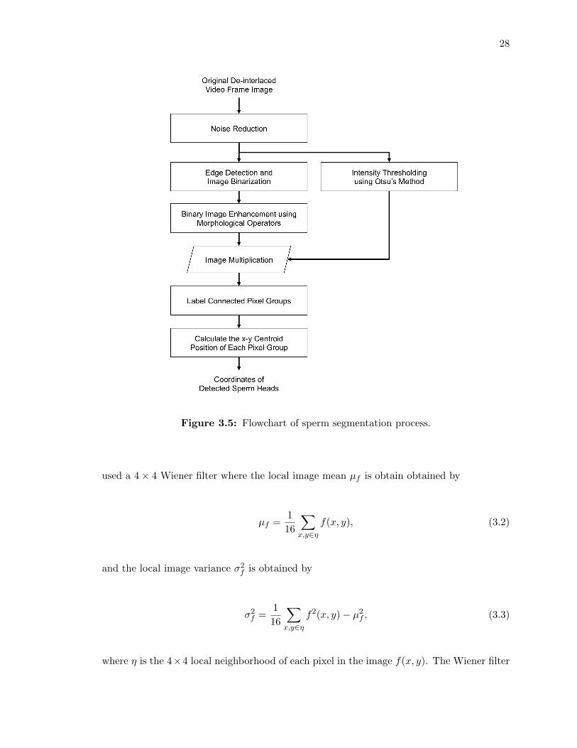
best. The complete segmentation process is outlined in Figure 3.5.

27
3.3 Edge Detection in Sperm Cell Images
This section presents a brief mathematical description of each step of the edge detection
process and shows the results of each step as applied to video frames obtained during our
sperm tracking experiments.
Prior to segmentation, each video frame is converted from its native RGB color video
frame to grayscale where each pixel has a value between 0 and 255. In standard image
processing texts [53], such a digital image is represented by a scalar function f(x, y) with
(x, y) 2 R2 and where the value of f(x, y) is the pixel grayscale value. The heart of image
processing is in the definition and application of specific image filters, denoted here by
h(x, y). By choosing an appropriate filter h(x, y), one can enhance or suppress selected
aspects of an image f(x, y). The application of an image filter h(x, y) to an image f(x, y)
is done using two-dimensional discrete convolution, given by
g(x, y) = f(x, y)⌦ h(x, y) =1X
m=�1
1X
n=�1f(x, y)h(x�m, y � n). (3.1)
Image Noise Reduction. The first step in our segmentation algorithm is to apply a filter
to reduce noise present in the video image. Image noise is caused by random electrical
disturbances in the video imaging system and is manifested as random light or dark pixels.
A simple way to reduce noise in an image is to replace each pixel by the average value of its
local neighboring pixels. A more sophisticated technique, such as a Wiener filter, exploits
the local statistical variation of pixel values in the neighborhood of each pixel. In this thesis,
we applied a standard Wiener filter hw
(x, y) which replaces each pixel value using estimates
of the local mean and variance in the neighborhood of each pixel. For imaging at ⇥200, we
28
Figure 3.5: Flowchart of sperm segmentation process.
used a 4⇥ 4 Wiener filter where the local image mean µf
is obtain obtained by
µf
=1
16
X
x,y2⌘f(x, y), (3.2)
and the local image variance �2f
is obtained by
�2f
=1
16
X
x,y2⌘f2(x, y)� µ2
f
, (3.3)
where ⌘ is the 4⇥4 local neighborhood of each pixel in the image f(x, y). The Wiener filter

29
hw
(x, y) is then constructed from these local estimates as
hw
(x, y) = µ+�2f
� ⌫2f
�2f
(f(x, y)� µf
), (3.4)
where ⌫f
is the average of all the local estimated variances. Applying the Wiener filter
yields a noise-reduced image fw
(x, y) given by
fw
(x, y) = f(x, y)⌦ hw
(x, y). (3.5)
Edge Detection and Image Binarization. The second step in our segmentation algo-
rithm is to detect the pixels in the noise-reduced image that correspond to edges separating
sperm from background pixels. To do this, we calculate the gradient of the image. The
gradient of the the noise-reduced image fw
(x, y) along the x and y direction can be approx-
imated using the Sobel method [53]. The Sobel method approximates the gradient along
the horizontal pixel rows by applying a 3⇥ 3 filter hx
(x, y) given by
hx
(x, y) =1
4
2
6
6
4
�1 0 +1
�2 0 +2
�1 0 +1
3
7
7
5
, (3.6)
and approximates the gradient along the vertical pixel columns by applying a 3 ⇥ 3 filter
and hy
(x, y) given by
hy
(x, y) =1
4
2
6
6
4
+1 +2 +1
0 0 0
�1 �2 �1
3
7
7
5
. (3.7)
30
The gradient of fw
(x, y) along x and y is then given by
dx
(x, y) =@f
w
(x, y)
@x= f
w
(x, y)⌦ hx
(x, y), (3.8)
and
dy
(x, y) =@f
w
(x, y)
@y= f
w
(x, y)⌦ hy
(x, y), (3.9)
and the image of the gradient magnitude of fw
(x, y) is given by
s(x, y) =q
d2x
(x, y) + d2y
(x, y). (3.10)
We wish to regard each point in s(x, y) whose value exceeds a cuto↵ threshold tc
as a point
corresponding to an edge between a sperm and the image background in fw
(x, y). In other
words, we wish to partition s(x, y) into a subset containing edges and non-edges. The choice
of tc
becomes a trade-o↵ between missing valid edges and creating noise-induced false edges.
One way to calculate tc
is by using the method described by Pratt in [53] given as
tc
= kc
p
< s2(x, y) >, (3.11)
where < s2(x, y) > is the mean of the image gradient magnitude squared, which approx-
imates the root mean square (RMS) of the image noise. Here, 0 < kc
< 1 is a tuning
parameter of the edge detection algorithm and o↵ers a trade-o↵ between detecting true
edges and detecting noise-induced false edges. In this thesis, we found that a typical value
of kc
= 0.75 worked well in all video images studied.
Using (3.11), we binarize fw
(x, y) by selecting those pixels from its gradient magnitude

31
s(x, y) which exceed the cuto↵ threshold tc
according to
b(x, y) = {s(x, y) : (s(x, y) > tc
)}. (3.12)
The result is a binary image b(x, y) whose elements are either 1 if the pixel is an edge or 0
if the pixel is a non-edge.
Image Enhancement using Morphological Operators. The third step of our sperm
segmentation algorithm is to refine the binary image b(x, y) by applying a sequence of
morphological dilation, closing and erosion operators. These enhancements help eliminate
pixels belonging to the sperm tail and debris and can enhance the separation between closely
spaced sperm. The first morphological operation applied is a dilation of the binarized image
gradient b(x, y) using a 1⇥ 3 horizontal binary structuring element sx
(x, y) followed by1 a
3⇥ 1 vertical binary structuring element sy
(x, y) given by
sx
(x, y) =h
1 1 1i
, (3.13)
and
sy
(x, y) =
2
6
6
4
1
1
1
3
7
7
5
. (3.14)
The resulting dilated binary image bd
(x, y) is obtained by
bd
(x, y) = (b(x, y)� sx
(x, y))� sy
(x, y), (3.15)
where � denotes Minkowski addition. After dilation, some holes may remain in the groups
1Since dilation is commutative (i.e., A�B = B �A), the order doesn’t matter.

32
of connected pixels belong to sperm. To close the holes, we apply a pixel-closing operation
on bd
(x, y) to obtain
bc
(x, y) = (bd
(x, y)��s1
(x, y)) s1
(x, y), (3.16)
where s1
(x, y) is a 3⇥ 3 binary matrix of 1’s and denotes Minkowski subtraction. Next,
an erosion of the surviving pixel groups is performed according to
be
(x, y) = bc
(x, y) �sd
(x, y), (3.17)
where sd
(x, y) is a 5⇥ 5 binary diamond structuring element given by
sd
(x, y) =
2
6
6
6
6
6
6
6
6
4
0 0 1 0 0
0 1 1 1 0
1 1 1 1 1
0 1 1 1 0
0 0 1 0 0
3
7
7
7
7
7
7
7
7
5
. (3.18)
Label Connected Pixel Groups. The fourth step of our sperm segmentation algorithm
is to label each connected pixel group in the final eroded binary image be
(x, y). This is done
by employing MATLAB’s built-in algorithm for labeling connected components assuming
4-connectivity. This creates a set of sub-images, each containing a group of connected pixels.
Sperm Head Localization. The fifth and final step of our sperm segmentation algo-
rithm is to calculate the centroid of each group of connected pixels. The coordinates of
the centroid of each connected pixel group are then regarded as the position of a detected
sperm head. We also calculate the area of the pixels in each pixel group in order to exclude

33
centroids belonging to pixel groups whose size far exceeds the size of a typical human sperm
head.

34
Algorithm 1 Sperm pixel segmentation using edge detection
1: for Each gray scale video frame image f(x, y) do2: Apply a Wiener filter h
w
(x, y) to remove image noise
fw
(x, y) = f(x, y)⌦ hw
(x, y)
3: Compute the row and column gradient of fw
(x, y) using Sobel filters hx
(x, y) andhy
(x, y)
dx
(x, y) =@f
w
(x, y)
@x= f
w
(x, y)⌦ hx
(x, y)
dy
(x, y) =@f
w
(x, y)
@y= f
w
(x, y)⌦ hy
(x, y)
and calculate the gradient magnitude
s(x, y) =q
d2x
(x, y) + d2y
(x, y)
4: Compute the gradient threshold tc
scaled by tuning parameter kc
tc
= kc
p
< s2(x, y) >
and form the binary image of s(x, y)
b(x, y) = {s(x, y) : s(x, y) > tc
}
5: Dilate the binary image b(x, y) using a vertical structuring element sx
(x, y) and ahorizontal structuring element s
y
(x, y) to obtain bd
(x, y)
bd
(x, y) = (b(x, y)� sx
(x, y))� sy
(x, y)
6: Close the holes in the binary image bd
(x, y) using a square matrix of ones s1
(x, y)
bc
(x, y) = (bd
(x, y)��s1
(x, y)) s1
(x, y)
7: Erode bc
(x, y) using a diamond structuring element sd
(x, y)
be
(x, y) = bc
(x, y) �sd
(x, y)
8: end for

35
3.4 Example Segmentation Results
The sperm segmentation process is illustrated in Figure 3.6 – Figure 3.16.
To demonstrate the edge-detection component of our segmentation algorithm, we show
each step applied to a sub-region of a ⇥200 video frame, depicted in Figure 3.6. Figure
3.6.A shows the original sub-region depicting several sperm in close proximity. Figure 3.6.B
shows the results of applying the Wiener filter to the original image to reduce image noise.
Figure 3.6.C is the image gradient calculated using the Sobel method. The pixels from
Figure 3.6.C are then subjected to dilation, closing and erosion operations (Figure 3.6.D,
Figure 3.6.E, and Figure 3.6.F, respectively). The connected pixels in Figure 3.6.F are then
labeled in Figure 3.6.G and the centroids of the labelled groups (depicted in Figure 3.6.H
by red crosses superimposed on the original sub-region image) are regarded as the positions
of the sperm heads.
Note that this edge-detection scheme can occasionally result in merged measurements
(note the two sperm mistakenly detected as a single sperm in the center of Figure 3.6.H).
This issue was addressed by combining the results of the edge-detection method with Otsu’s
method, which does a better job at discerning multiple sperm in close proximity. Using two
⇥200 frames (A and B) collected from two di↵erent videos obtained from our sperm tracking
experiments (Figures 3.7 and 3.8), the output of the edge-detection algorithm is shown for
both in Figures 3.9 and 3.10. In these figures, the edges of sperm are detected evenly
across the image despite local variations in the grayscale value of each frame’s background.
However, there is a tendency for the pixels of nearby sperm to be coalesced into blobs,
which results in merged measurements. In contrast, applying Otsu’s method on the original
noise-reduced image frames (see Figures 3.11 and 3.12), results in improved identification
of pixels belonging to nearby sperm and helps avoid merged measurements. However, since

36
Otsu’s method uses the global image frame grayscale statistics to calculate its detection
threshold value, it can sometimes cause portions of unevenly illuminated background image
to be detected. When we multiply these two results together, we get the benefits of both
(see Figures 3.13 and 3.14). Calculating the centroids of the multiplied images yields the
final results depicted in Figures 3.15 and 3.16.
Once the centroids of each sperm are identified, the x-y coordinates are converted to
microns by applying a scale factor. This pixel-to-micron scale factor was determined by
imaging a sample superimposed with a digital boresight applied by the microscope image-
capture software. The boresight had a known diameter of 12 µm at ⇥400 magnification
and using recorded videos had a measured diameter of 28 pixels. This corresponds to a
pixel-to-micron scale factor of 0.429 µm/pixel at ⇥400 and 0.857 µm/pixel at ⇥200. Sub-
micron variability was observed after repeated imaging and measurement of the boresight
diameter, indicating a spatial resolution for each digital microscopic image of <1 pixel = <
0.857 µm.
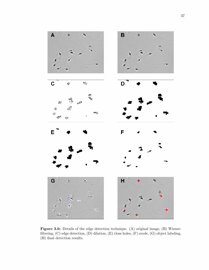
37
Figure 3.6: Details of the edge detection technique. (A) original image, (B) Wiener-filtering, (C) edge detection, (D) dilation, (E) close holes, (F) erode, (G) object labeling,(H) final detection results.

38
Figure 3.7: Original video frame A.
Figure 3.8: Original video frame B.

39
Figure 3.9: Morphologically enhanced detected edges in video frame A.
Figure 3.10: Morphologically enhanced detected edges in video frame B.
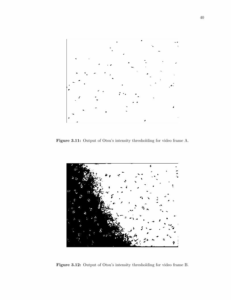
40
Figure 3.11: Output of Otsu’s intensity thresholding for video frame A.
Figure 3.12: Output of Otsu’s intensity thresholding for video frame B.
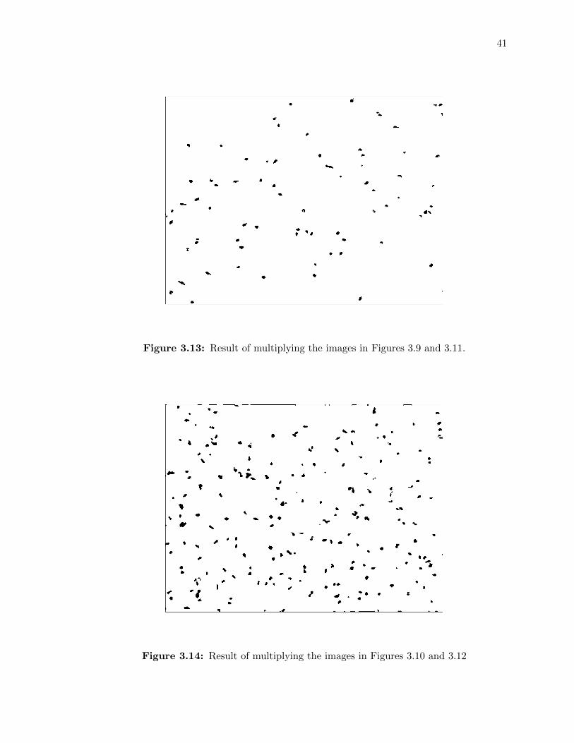
41
Figure 3.13: Result of multiplying the images in Figures 3.9 and 3.11.
Figure 3.14: Result of multiplying the images in Figures 3.10 and 3.12

42
Figure 3.15: Final segmentation results for video frame A.
Figure 3.16: Final segmentation results for video frame B.

43
Chapter 4: Multi-Sperm Tracking
In this chapter, we present and discuss several multi-target tracking algorithms and their
application to multi-sperm tracking in time-lapse images. We begin by presenting the
two dimensional two state (position-velocity) Kalman filter with measurement gating for
tracking targets assuming zero mean white Gaussian process and measurement noise dis-
turbances. Next, the PDAF and the JPDAF are presented and their relative strengths and
weaknesses discussed. Special attention is given to the computationally expensive process of
enumerating every feasible joint association event for the JPDAF. A simpler approach that
rapidly identifies the most highly probable joint events based on Murty’s method for finding
the M -best ranked assignments is then demonstrated. Track partitioning using k-means
clustering to enable additional computational throughput is then discussed, followed by a
review of classical track management logic for the initiation, continuation and deletion of
target tracks based on the concept of track score.
4.1 Kalman Filter for Sperm Tracking
Kalman filters with reduced state kinematic models are used extensively in real-time tar-
get tracking applications [54, 55, 56, 57, 58, 59, 60]. In the formulation of these filters,
higher-order target states like acceleration and jerk, which often vary unpredictably and
do not last long enough to be observed or estimated during maneuvers, are often neglected
[61]. Instead, additive white plant noise is used in the filter plant model to account for
un-modeled target states.

44
Discrete White Noise Acceleration (DWNA) Target Model. One of the most widely
used reduced state kinematic models for target motion is the two state (position-velocity)
discrete white noise acceleration (DWNA) model. The DWNA model for the motion of a
target t moving in two dimensions is given by
xt
(k + 1) = Fxt
(k) +Gwt
(k), (4.1)
where xt
(k) is the 4 ⇥ 1 target t state vector at time k and wt
(k) is the 2 ⇥ 1 zero mean
piecewise constant random target acceleration vector with covariance matrix W (k). A
measurement zt
(k) (target position plus noise) is obtained every T seconds given by
zt
(k) = Hxt
(k) + nt
(k), (4.2)
where nt
(k) is the 2 ⇥ 1 zero mean additive white position noise vector with covariance
matrix N(k). The constant system dynamics matrix F , system input gain matrix G and
measurement matrix H are given by, respectively,
F =
2
6
6
6
6
6
4
1 0 T 0
0 1 0 T
0 0 1 0
0 0 0 1
3
7
7
7
7
7
5
, (4.3)
G =
2
6
6
6
6
6
4
T 2/2 0
0 T 2/2
T 0
0 T
3
7
7
7
7
7
5
, (4.4)

45
and
H =
"
1 0 0 0
0 1 0 0
#
. (4.5)
In reality, multiple measurements may be available at time k and the tracker doesn’t know
which measurement belongs to target t. Therefore, in the sequel we denote by zj
(k) the
j�th measurement received at time k and by tj
the index of the target to which measure-
ment j is associated.
DWNA Kalman Filter. For linear kinematic target models with zero mean white noise
inputs, the Kalman filter is the optimal minimum mean square error (MMSE) state estima-
tor [57]. The Kalman filter for estimating the state of a target tj
from a sequence of noisy
position measurements zj
(k) assuming the state and measurement model given by Equa-
tions (4.1) and (4.2) is now presented. Here, the predicted target state vector xtj (k|k � 1)
is given by
xtj (k|k � 1) = Fx
tj (k � 1|k � 1), (4.6)
and the predicted measurement vector ztj (k|k � 1) is given by
ztj (k|k � 1) = Hx
tj (k|k � 1), (4.7)
where the notation (k|k�1) indicates a quantity at time k given a measurement at time k�1.
The di↵erence between the measurement zj
(k) and the predicted measurement ztj (k|k� 1)
is called the measurement residual or the innovation vector and is given by
⌫jtj (k) = z
j
(k)� ztj (k|k � 1), (4.8)

46
and has covariance matrix Stj (k) where
Stj (k) = HP
tj (k|k � 1)HT +N(k). (4.9)
The predicted target state estimation error covariance matrix Ptj (k|k � 1) is given by
Ptj (k|k � 1) = FP
tj (k � 1|k � 1)F T +Q(k � 1), (4.10)
where Q(k � 1) is the process noise covariance matrix given by
Q(k � 1) = GW (k � 1)GT . (4.11)
The estimated target state vector xtj (k|k) and state estimation error covariance matrix
Ptj (k|k) are then given by
xtj (k|k) = x
tj (k|k � 1) +Ktj (k)⌫jtj (k), (4.12)
and
Ptj (k|k) = P
tj (k|k � 1)�Ktj (k)HP
tj (k|k � 1), (4.13)
where Ktj (k) is the Kalman filter gain matrix
Ktj (k) = P
tj (k|k � 1)HTStj (k)
�1. (4.14)
47
Measurement Gating. In practice, the measurement zj
(k) is only processed by the filter
if it is validated or gated by the track. That is, if the measurement falls within the two
dimensional error ellipsoid defined by the filter-calculated residual covariance matrix Stj (k),
i.e.,
⌫jtj (k)
TStj (k)
�1⌫jtj (k) �, (4.15)
where � is the gate threshold. The value of � is chosen based on the probability PG
that
the gate would contain a measurement if the target were detected by the sensor [58]. Under
the zero mean white noise assumption of the state estimation and measurement errors, the
quantity ⌫jtj (k)
TStj (k)
�1⌫jtj (k) is a Chi-squared distributed random variable with degrees
of freedom equal to the dimension of the measurement residual vector ⌫jtj (k), in this case
2. This quantity is also referred to as the normalized innovations squared, Mahalanobis
distance, or the normalized statistical distance between the predicted measurement ztj (k|k�
1) and the actual measurement zj
(k). Based on the cumulative distribution function for a
Chi-squared random variable with 2 degrees of freedom, a gate probability of PG
= 0.95
corresponds to � = 5.9915 and a gate probability PG
= 0.9997 corresponds to � = 16.2235.
Colloquially,p� is sometimes referred to as the number of sigmas of a validation gate [32].
Depending on the size of Stj (k), a measurement may satisfy Equation (4.15) but, be-
cause of its relative position with respect to the predicted target position, may result in an
excessively large (sometimes non-physical) velocity. If this occurs, it can lead to track loss.
For this reason, an additional velocity gating criterion may be applied of the form
k⌫jtj (k)kT
Vmax
, (4.16)
where Vmax
is the maximum possible target velocity (for moving sperm imaged at 15 frames
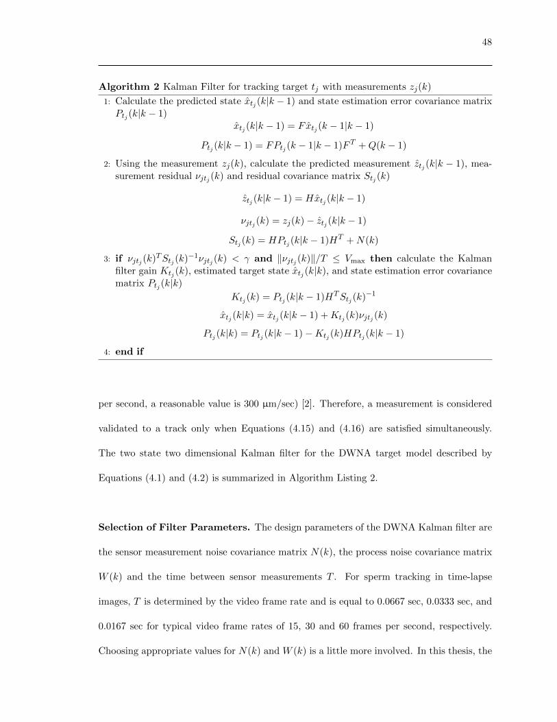
48
Algorithm 2 Kalman Filter for tracking target tj
with measurements zj
(k)
1: Calculate the predicted state xtj (k|k � 1) and state estimation error covariance matrix
Ptj (k|k � 1)
xtj (k|k � 1) = Fx
tj (k � 1|k � 1)
Ptj (k|k � 1) = FP
tj (k � 1|k � 1)F T +Q(k � 1)
2: Using the measurement zj
(k), calculate the predicted measurement ztj (k|k � 1), mea-
surement residual ⌫jtj (k) and residual covariance matrix S
tj (k)
ztj (k|k � 1) = Hx
tj (k|k � 1)
⌫jtj (k) = z
j
(k)� ztj (k|k � 1)
Stj (k) = HP
tj (k|k � 1)HT +N(k)
3: if ⌫jtj (k)
TStj (k)
�1⌫jtj (k) < � and k⌫
jtj (k)k/T Vmax
then calculate the Kalmanfilter gain K
tj (k), estimated target state xtj (k|k), and state estimation error covariance
matrix Ptj (k|k)
Ktj (k) = P
tj (k|k � 1)HTStj (k)
�1
xtj (k|k) = x
tj (k|k � 1) +Ktj (k)⌫jtj (k)
Ptj (k|k) = P
tj (k|k � 1)�Ktj (k)HP
tj (k|k � 1)
4: end if
per second, a reasonable value is 300 µm/sec) [2]. Therefore, a measurement is considered
validated to a track only when Equations (4.15) and (4.16) are satisfied simultaneously.
The two state two dimensional Kalman filter for the DWNA target model described by
Equations (4.1) and (4.2) is summarized in Algorithm Listing 2.
Selection of Filter Parameters. The design parameters of the DWNA Kalman filter are
the sensor measurement noise covariance matrix N(k), the process noise covariance matrix
W (k) and the time between sensor measurements T . For sperm tracking in time-lapse
images, T is determined by the video frame rate and is equal to 0.0667 sec, 0.0333 sec, and
0.0167 sec for typical video frame rates of 15, 30 and 60 frames per second, respectively.
Choosing appropriate values for N(k) and W (k) is a little more involved. In this thesis, the
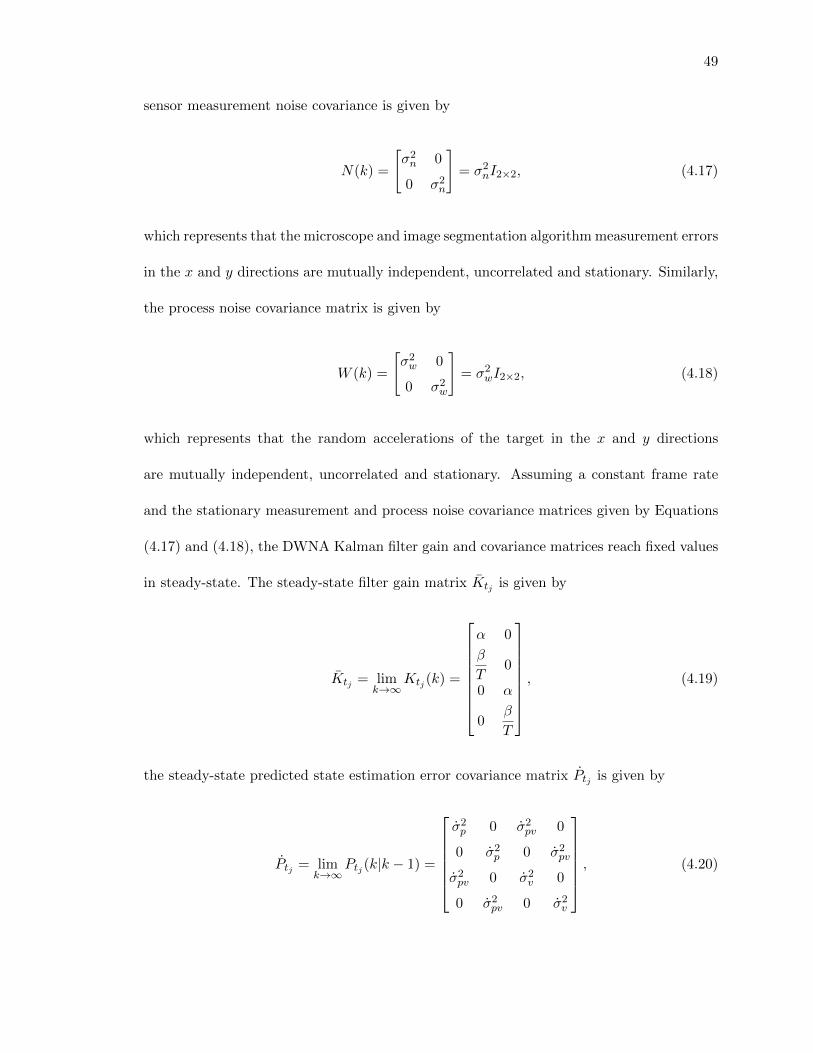
49
sensor measurement noise covariance is given by
N(k) =
"
�2n
0
0 �2n
#
= �2n
I2⇥2
, (4.17)
which represents that the microscope and image segmentation algorithm measurement errors
in the x and y directions are mutually independent, uncorrelated and stationary. Similarly,
the process noise covariance matrix is given by
W (k) =
"
�2w
0
0 �2w
#
= �2w
I2⇥2
, (4.18)
which represents that the random accelerations of the target in the x and y directions
are mutually independent, uncorrelated and stationary. Assuming a constant frame rate
and the stationary measurement and process noise covariance matrices given by Equations
(4.17) and (4.18), the DWNA Kalman filter gain and covariance matrices reach fixed values
in steady-state. The steady-state filter gain matrix Ktj is given by
Ktj = lim
k!1K
tj (k) =
2
6
6
6
6
6
6
6
4
↵ 0
�
T0
0 ↵
0�
T
3
7
7
7
7
7
7
7
5
, (4.19)
the steady-state predicted state estimation error covariance matrix Ptj is given by
Ptj = lim
k!1Ptj (k|k � 1) =
2
6
6
6
6
6
4
�2p
0 �2pv
0
0 �2p
0 �2pv
�2pv
0 �2v
0
0 �2pv
0 �2v
3
7
7
7
7
7
5
, (4.20)

50
and the steady-state updated state estimation error covariance matrix Ptj is given by
Ptj = lim
k!1Ptj (k|k) =
2
6
6
6
6
6
4
�2p
0 �2pv
0
0 �2p
0 �2pv
�2pv
0 �2v
0
0 �2pv
0 �2v
3
7
7
7
7
7
5
. (4.21)
Substituting Equations (4.20) and (4.17) into (4.9) yields the steady-state residual covari-
ance matrix Stj given by
Stj = lim
k!1Stj (k) =
"
�2s
0
0 �2s
#
=
"
�2p
+ �2n
0
0 �2p
+ �2n
#
. (4.22)
Substituting Equation (4.22) and (4.19) into (4.14) yields the two relationships
↵ =�2p
�2p
+ �2n
, (4.23)
and
� =
�2pv
�2p
+ �2n
!
T. (4.24)
Recalling from Equation (4.22) that �2s
= �2p
+ �2n
, we can re-arrange Equation (4.23) and
take the square root to obtain
�s
�n
=1p
1� ↵, (4.25)
where �s
/�n
is the normalized residual error. This expression is useful because it relates
the size of the validation gate to the sensor noise and filter position gain ↵.
In [55], Kalata showed that the steady-state DWNA Kalman filter gain and covariance
matrices are completely determined by the single dimensionless quantity known as the target

51
tracking index, denoted by ⇤, according to
⇤2 =�2w
T 4
�2n
=�2
1� ↵ , (4.26)
and the filter gains obey the Kalata relation [57] given by
� = 2(2� ↵)� 4p1� ↵. (4.27)
Substituting (4.27) into (4.26) and solving for ↵ yields
↵ = �1
8
n
⇤2 + 8⇤� (⇤+ 4)p
⇤2 + 8⇤o
, (4.28)
which is plotted for a range of tracking index values in Figure 4.1. In addition, the normal-
ized residual error is also plotted as a function of tracking index. Equations (4.26)–(4.28)
have been used extensively in the literature to design and characterize Kalman filters for
target tracking applications [58, 57, 59, 60, 62].

52
Figure 4.1: Steady-state DWNA ↵-� filter gains and normalized residual error vstracking index ⇤.

53
In the formulation of the DWNA target model, the target acceleration is assumed to
be a zero mean random white process. In reality, however, realistic target maneuvers
violate the zero mean white noise assumption. Real target maneuvers are not random white
noise accelerations, but deterministic accelerations with unknown magnitude and direction
and unknown onset time and duration. A common design problem in the target tracking
literature is: how should the white process noise �2w
be chosen for a given application?
A prevalent method for designing DWNA Kalman filters is to select the value of �2w
via empirical tuning, which is often a di�cult task [61]. Another method is to choose �2w
in some relation to a-priori knowledge about the target maneuver capability, such as the
maximum acceleration of the target Amax
. According to Blair and Bar-Shalom in [63], one
should choose �2w
= A2
max
or A2
max
/4. According to Blackman [58], it is common to choose
�2w
= A2
max
/9. These rule-of-thumb schemes are only approximations that attempt to relate
the model random acceleration to the real target acceleration [64], but each scheme yields
a di↵erent value for �2w
and hence di↵erent filter performance.
In applying the DWNA Kalman filter to sperm tracking, a further question must be
asked: what exactly is the target? Although the sperm head is the most recognizable
feature of the sperm and most easily segmented, it wiggles sinusoidally about an average
path traced by a non-wiggling point typically located somewhere on the sperm mid-piece.
Are we tracking the sperm head or are we tracking the average position traced out by the
sperm? Clearly, to measure sperm motility parameters we must reconstruct and analyze the
path traced out by the sperm head. However, predicting the position of a sperm head with
any accuracy would require either a high video frame rate or a highly nonlinear model that
accounts for the complex hydrodynamic interactions between the head, tail and surrounding
media [65], or both.

54
In this thesis, we explore a novel solution to the problem of selecting filter parameters:
(1) we use the DWNA Kalman filter to predict and estimate the mean path about which the
sperm head wiggles in order to maintain track and (2) we use the raw position measurements
associated (i.e., validated) to the track in order to reconstruct the complex path traced by
the sperm head and to measure its motility parameters. This is accomplished by choosing
�2w
approximately equal to the acceleration of the average sperm swimming path, which is
significantly less than the acceleration of the sperm head itself.
To illustrate this approach, consider the two sperm trajectories and their average swim-
ming paths shown in Figure 4.2 and 4.3. These trajectories were collected from our sperm
tracking experiments using videos imaged at 15 frames per second and a 5-point moving
average was used to obtain the average swimming paths. The trajectory in Figure 4.2 is
a large circular path comprised of 240 track points (16 sec long) while the trajectory in
Figure 4.3 is an “S”-shaped meandering path comprised of 136 track points (9 sec long).
The average deviation of the sperm head position between consecutive track points was
empirically found to be 4.3 and 4.6 µm for the circular and meandering paths, respectively.
The acceleration necessary to move the sperm head a distance of 4.3 µm in T = 1/15 sec
is approximately 2(4.3 µm)/T 2 = 1,935 µm/sec2 and to move a distance of 4.6 µm is ap-
proximately 2(4.6 µm)/T 2 = 2,070 µm/sec2. Thus, for both trajectories the sperm head
acceleration is approximately 2,000 µm/sec2. Assuming the maximum acceleration of the
average swimming path is significantly less than the acceleration of the sperm head (namely,
one-tenth) we obtain for �2w
a value of 200 µm/sec2. The wobbling position of the sperm
head was regarded as additional sensor noise by selecting for �n
a value of 4 µm in each
direction or �n
= 4p2 µm. The tracking index for �
n
= 4p2µm, �
w
= 200 µm/sec2, and
T = 0.0667 sec (assuming a frame rate of 15 frames per second) is ⇤ = 0.1571. This corre-

55
sponds to a normalized residual error ratio of�s
�n
= 1.3223 and thus a validation gate radius
ofp��
s
= 18.3091 µm for � = 5.9915 (i.e., PG
= 0.95) and 30.1282 µm for � = 16.2235
(i.e., PG
= 0.9997).
The purpose of this approach to filter parameter selection is to ensure that measure-
ments of the sperm head are detected inside the validation gate centered at the predicted
average sperm position – i.e., to ensure that track is maintained. A track is more likely
to be lost if a detected sperm head lies outside the track validation gate. In order to
evaluate how the above choice of filter parameters satisfies this objective, we applied the
DWNA filter to simulated sperm swimming paths and calculated the normalized innova-
tions squared using Equation 4.15 averaged over 100 Monte Carlo trajectories at each time
k. In the two-dimensional tracking problem, the theoretical NIS is chi-squared distributed
random variable with two degrees of freedom. The average NIS is plotted in figure 4.4
along with the intervals within which the NIS is expected to fall with 95% confidence. In
a perfectly matched filter (i.e., when the sample innovation covariance exactly matches the
filter-calculated innovation covariance) the average NIS would fall between the upper and
lower confidence levels. Observe that the average NIS is below the lower confidence level;
this signifies that this set of filter parameters yields a residual covariance matrix that is
larger than the sample residual error covariance. In other words, sperm head detections
are likely to fall within the validation gate centered at the predicted track position. This is
demonstrated in Figure 4.5 which shows the true position, predicted position and validation
gate for one of the 100 Monte Carlo simulated sperm trajectories. At each point, the true
sperm head position is contained within the validation gate.

56
Figure 4.2: Circular sperm trajectory.
Figure 4.3: Meandering sperm trajectory.
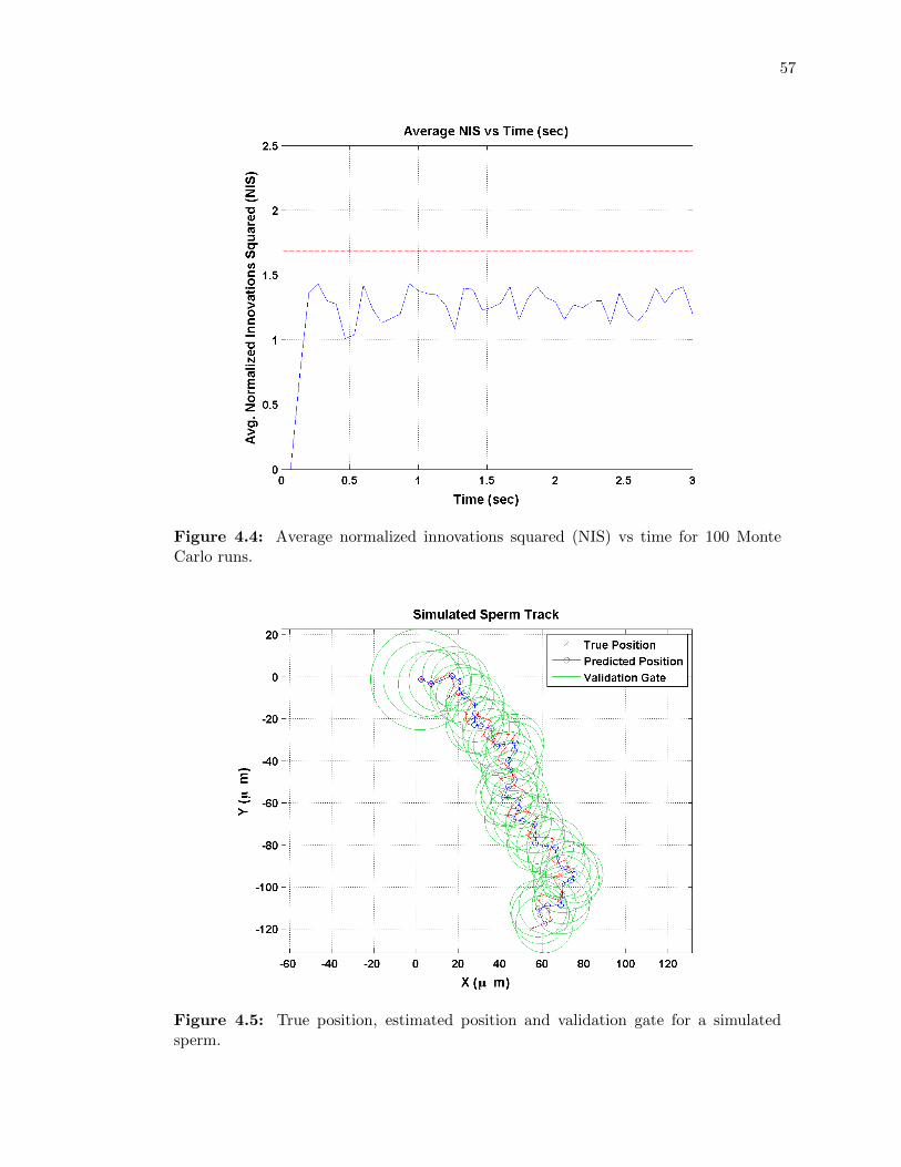
57
Figure 4.4: Average normalized innovations squared (NIS) vs time for 100 MonteCarlo runs.
Figure 4.5: True position, estimated position and validation gate for a simulatedsperm.

58
4.2 The Probabilistic Data Association Filter (PDAF)
In the Kalman filter presented in the previous section, no provision was made for the
possibility that multiple measurements may be validated by the track filter. In such a
case, a decision process is needed in order to choose which measurement or combination
of measurements should be used to update the track filter. In this section we describe the
PDAF, which is the multi-measurement extension of the Kalman filter and is designed for
tracking single targets in clutter [66].
The basic approach of the PDAF is to consider at every scan of data the probability that
each validated measurement came either from the target of interest or from clutter. All of
the measurements validated by the track filter are then combined into a single probability-
weighted average measurement which is used to update the track. To develop the equations
for the PDAF, consider a set of m measurements received at time k which we denote by
Z(k) = {zj
(k)}mj=1
, (4.29)
and the set of all measurements up to and including time k which we denote by
Zk = {Z(i)}ki=1
. (4.30)
In the standard parametric formulation of the PDAF assuming a Poisson clutter model,
the marginal probability �jt
(k) that measurement zj
(k) is associated to track t at time k is

59
given by [40]
�jt
(k) =
8
>
>
>
>
>
>
>
>
>
>
<
>
>
>
>
>
>
>
>
>
>
:
Ljt
(k)
1� P t
D
PG
+P
m
j=1
Ljt
(k), if j = 1 . . .m
1� P t
D
PG
1� P t
D
PG
+P
m
j=1
Ljt
(k), j = 0
(4.31)
where j = 0 means that no measurements were validated by the track and P t
D
is the target
detection probability. The likelihood ratio Ljt
(k) that the measurement zj
(k) originated
from target t rather than from clutter is given by
Ljt
(k) = ��1ftj [zj(k)]P
t
D
, (4.32)
where ftj [.] denotes the Gaussian pdf with argument z
j
(k), mean ztj (k|k�1), and covariance
Stj (k) given by
ftj [zj(k)] = |2⇡S
tj (k)|�1/2 exp
✓
�1
2⌫jtj (k)
TStj (k)
�1⌫jtj (k)
◆
, (4.33)
and |.| denotes the determinant operator. In equation (4.32), the expected number of
measurements due to clutter per unit area of the surveillance space per scan of data is
assumed to be Poisson distributed with mean �. In practice, � is a design parameter and a
typical value representing infrequent clutter detections is � = 1⇥ 10�6 per unit area.
Once the marginal probabilities �jt
(k) have been calculated for all of the measurements
validated by track t, a probability-weighted combined residual ⌫t
(k) is calculated according
60
to
⌫t
(k) =m
X
j=1
�jt
(k)⌫jtj (k), (4.34)
and used to update the state in track t’s Kalman filter according to
xt
(k|k) = xt
(k|k � 1) +Kt
(k)⌫t
(k), (4.35)
where the Kalman filter gain is computed as before in Equation (4.14). Unlike the standard
Kalman filter, in the PDAF the updated state estimation error covariance matrix Pt
(k|k)
is increased to reflect the additional error due to measurement origin uncertainty according
to
Pt
(k|k) = �0t
(k)Pt
(k|k � 1) + [1� �0t
(k)]P c
t
(k|k) + Pt
(k). (4.36)
In Equation (4.36), �0t
(k) is the probability that none of the measurements is correct which
is given by equation (4.31) to be equal to
�0t
(k) =1� P
D
PG
1� P t
D
PG
+P
m
j=1
Ljt
(k), (4.37)
the matrix P c
t
(k|k) is the updated state estimation error covariance that would be obtained
in the absence of measurement origin uncertainty given by
P c
t
(k|k) = Pt
(k|k � 1)�Kt
(k)St
(k)Kt
(k)T , (4.38)
and the matrix Pt
(k) is the spread of the innovations given by
Pt
(k) = Kt
(k)
2
4
m
X
j=1
�jt
(k)⌫jtj (k)⌫jtj (k)
T � ⌫t
(k)⌫t
(k)T
3
5Kt
(k)T . (4.39)

61
Figure 4.6: Measurement-to-track association conflicts.
4.3 The Joint Probabilistic Data Association Filter (JPDAF)
Although the PDAF performs well when tracking a single target in clutter, it is ill-suited
for tracking multiple targets. In particular, the PDAF performs very poorly when tracking
multiple targets in close proximity or whose paths intersect (for example, Figure 4.6). This
is expected, since the PDAF was derived assuming only two measurement origin hypotheses:
either the measurement originated from the target of interest, or it originated from clutter.
No consideration is made by the PDAF for the possibility that a measurement originated
from another target, which may or may not already be in track. In such a scenario, it is
possible that each measurement belongs to a di↵erent track. It is also possible that some
(or all) of the measurements are clutter. In any situation involving a set of measurements
in conflict with a set of tracks there are many possible association hypotheses. The problem
to solve is: which hypothesis is correct?
The multi-target extension of the PDAF which addresses this problem is called the

62
joint probabilistic data association filter (JPDAF) [41, 32]. The key di↵erence between the
PDAF and the JPDAF is that in the JPDAF the marginal measurement-to-track association
probabilities �jt
(k) are calculated jointly across all targets and validated measurements. In
order to do this, the JPDAF must enumerate every feasible joint association event – i.e.,
every feasible combination of association between every target and measurement. This has
the advantage that when multiple measurements are validated by a track, the probability-
weighted combined residual correctly discounts the contribution of measurements shared by
nearby tracks, a feature which the PDAF lacks.
A feasible joint association event is an assignment of measurements to tracks or to clutter
satisfying two requirements: (R1) a measurement can originate from only a single target or
from clutter and (R2) a target can give rise to no more than one measurement [41, 32, 67].
For m measurements and n tracks, the probability of the joint association event ✓(k) given
the measurements up to time k is given by [68]
P{✓(k)|Zk} =1
c
m
Y
j=1
{��1ftj [zj(k)]}⌧j(✓)
n
Y
t=1
(P t
D
)�t(✓)(1� P t
D
)1��t(✓), (4.40)
where ⌧j
(✓) is the binary measurement association indicator, �t
(✓) is the binary target detec-
tion indicator, and c is a normalizing constant. In equation (4.40), ⌧j
(✓) = 1 if measurement
j is associated with any target in the event ✓, and �t
(✓) = 1 if target t is associated with
any measurement in the event ✓ (they are equal to zero otherwise). The marginal proba-
bility �jt
(k) that measurement j is associated with target t is then given by summing the
probabilities of the joint events where this target-to-measurement association occurs. The
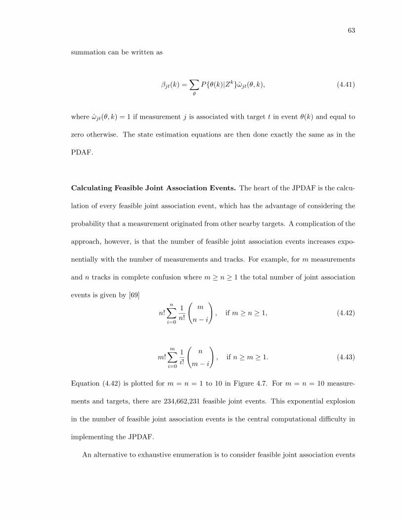
63
summation can be written as
�jt
(k) =X
✓
P{✓(k)|Zk}!jt
(✓, k), (4.41)
where !jt
(✓, k) = 1 if measurement j is associated with target t in event ✓(k) and equal to
zero otherwise. The state estimation equations are then done exactly the same as in the
PDAF.
Calculating Feasible Joint Association Events. The heart of the JPDAF is the calcu-
lation of every feasible joint association event, which has the advantage of considering the
probability that a measurement originated from other nearby targets. A complication of the
approach, however, is that the number of feasible joint association events increases expo-
nentially with the number of measurements and tracks. For example, for m measurements
and n tracks in complete confusion where m � n � 1 the total number of joint association
events is given by [69]
n!n
X
i=0
1
n!
m
n� i
!
, if m � n � 1, (4.42)
m!m
X
i=0
1
i!
n
m� i
!
, if n � m � 1. (4.43)
Equation (4.42) is plotted for m = n = 1 to 10 in Figure 4.7. For m = n = 10 measure-
ments and targets, there are 234,662,231 feasible joint events. This exponential explosion
in the number of feasible joint association events is the central computational di�culty in
implementing the JPDAF.
An alternative to exhaustive enumeration is to consider feasible joint association events

64
Figure 4.7: Number of feasible joint association events for m = n = 1 to 10.
as solutions to classical assignment problems. In a multi-target tracking problem having
m measurements and n targets, a feasible joint association event can be expressed as the
solution to the m⇥ n association matrix A given by
A = [ajt
] =
8
>
>
>
>
<
>
>
>
>
:
� ln(��1ftj [zj(k)]), if measurement j is validated by track t
1, otherwise
(4.44)
In Equation (4.44), each element ajt
of A is equal to the negative log likelihood ratio (NLLR)
that a validated measurement j is associated with track t at time k as opposed to clutter
and equal to infinity if measurement j not validated by track t. A solution to A is an
assignment of measurements to tracks that satisfies feasibility requirements (R1) and (R2).
An optimal solution to A is a solution A⇤ that satisfies feasibility requirements (R1) and

65
Figure 4.8: Example: five targets and five measurements in conflict.
(R1) and where the value of the sum of the assignments is the minimum over every other
permutation of legal assignments. A number of popular methods for solving the optimal
assignment problem can be used here, among which are the Munkres algorithm, the Jonker-
Volgenant-Castanon (JVC) algorithm and the auction algorithm [33]. In this thesis, we use
the Munkres algorithm which is summarized in Algorithm Listing 3 (adapted from [70] to
match our notation).
As an example, consider the scenario depicted in Figure 4.8 in which four targets t1
, t2
,
t3
, and t4
are in conflict with four measurements z1
, z2
, z3
, and z4
. The association matrix
A0
for this scene is given by
A0
=
2
6
6
6
6
6
4
�12.5908 �10.7781 1 �10.0680
�10.5315 �12.7375 �9.9715 �11.9809
�12.0178 �12.2701 �11.6031 �12.8759
1 1 �12.4983 �10.2984
3
7
7
7
7
7
5
. (4.45)

66
Algorithm 3 Munkres algorithm for finding an optimal assignment for the matrix A
1: For each row of the matrix A subtract the value of the smallest element from eachelement in the row.
2: For each column of the resulting matrix subtract the value of the smallest element fromeach element in the column.
3: Find a zero, Z, of the matrix. If there is no starred zero in its row nor its column, starZ. Repeat for each zero of the matrix. Go to step 4.
4: Cover every column containing a 0⇤. If all columns are covered, the starred zeros formthe desired independent set; Exit. Otherwise, go to step 5.
5: Choose a noncovered zero and prime it; then consider the row containing it. If thereis no starred zero Z in this row, go to step 6. If there is a starred zero Z in this row,cover this row and uncover the column of Z. Repeat until all zeros are covered. Go tostep 7.
6: There is a sequence of alternating starred and primed zeros constructed as follows: letZ0
denote the uncovered 00. Let Z1
denote the Z⇤ in Z 00
s column (if any). Let Z2
denotethe 00 in Z 0
1
s row. Continue in a similar way until the sequence stops at 00, Z2k
, whichhas no 0⇤ in its column. Unstar each starred zero of the sequence, and star each primedzero of the sequence. Erase all primes and uncover every line. Return to step 4.
7: Let h denote the smallest noncovered element of the matrix; it will be positive. Addh to each covered row; then subtract h from each uncovered column. Return to step 5without altering any asterisks, primes, or covered lines.
Applying the Munkres algorithm to A we obtain the optimal assignment A⇤0
given by
A⇤0
=
2
6
6
6
6
6
4
�12.5908 �10.7781 1 �10.0680
�10.5315 �12.7375 �9.9715 �11.9809
�12.0178 �12.2701 �11.6031 �12.8759
1 1 �12.4983 �10.2984
3
7
7
7
7
7
5
, (4.46)
where the bold blue elements indicate the assignments. The value or cost of an assignment
is the sum of the individual assignments. The optimal assignment A⇤0
is the assignment with
minimum cost, in this case -50.7025. The solution A⇤0
is a feasible joint association event
which we denote by
✓0
= (t1
, z1
)(t2
, z2
)(t3
, z4
)(t4
, z3
). (4.47)
To find additional feasible joint association events, one can create new sub-problems from
67
A0
by selecting an arbitrary association (i.e., an element in A0
) and removing it from con-
sideration (i.e., by setting it equal to infinity) and then re-run the Munkres algorithm to
find a new optimal assignment.
Murty’s Method for Finding the M-Best Ranked Assignments. In [71], Murty
presented a method for finding the set of M -best assignments of A ranked in order of
increasing cost. In [67], Cox recognized that Murty’s method could be applied to multi-
target tracking on order to identify the most highly probable feasible joint association events.
The essence of Murty’s method is rather than creating new sub-problems by removing
elements from A selected arbitrarily, one removes from A elements corresponding to an
optimal assignment beginning with the initial optimal assignment. A complete description
of Murty’s method, adapted to our notation, is provided in Algorithm Listing 4 and an
original implementation of the method written in MATLAB developed for this thesis is
provided in Appendix B.
Applying Murty’s method to A0
, we obtain the four next best solutions A⇤1
, A⇤2
, A⇤3
, and
A⇤4
and four corresponding feasible joint association events ✓1
, ✓2
, ✓3
, and ✓4
, given by
A⇤1
=
2
6
6
6
6
6
4
�12.5908 �10.7781 1 �10.0680
�10.5315 �12.7375 �9.9715 �11.9809
�12.0178 �12.2701 �11.6031 �12.8759
1 1 �12.4983 �10.2984
3
7
7
7
7
7
5
(4.48)
✓1
= (t1
, z1
)(t2
, z3
)(t3
, z4
)(t4
, z2
), cost = � 49.3401 (4.49)

68
A⇤2
=
2
6
6
6
6
6
4
�12.5908 �10.7781 1 �10.0680
�10.5315 �12.7375 �9.9715 �11.9809
�12.0178 �12.2701 �11.6031 �12.8759
1 1 �12.4983 �10.2984
3
7
7
7
7
7
5
(4.50)
✓2
= (t1
, z2
)(t2
, z2
)(t3
, z4
)(t4
, z1
), cost = � 47.3216 (4.51)
A⇤3
=
2
6
6
6
6
6
4
�12.5908 �10.7781 1 �10.0680
�10.5315 �12.7375 �9.9715 �11.9809
�12.0178 �12.2701 �11.6031 �12.8759
1 1 �12.4983 �10.2984
3
7
7
7
7
7
5
(4.52)
✓3
= (t1
, z2
)(t2
, z1
)(t3
, z4
)(t4
, z2
), cost = � 47.2751 (4.53)
and
A⇤4
=
2
6
6
6
6
6
4
�12.5908 �10.7781 1 �10.0680
�10.5315 �12.7375 �9.9715 �11.9809
�12.0178 �12.2701 �11.6031 �12.8759
1 1 �12.4983 �10.2984
3
7
7
7
7
7
5
(4.54)
✓4
= (t1
, z1
)(t2
, z2
)(t3
, z3
)(t4
, z4
), cost = � 47.2298 (4.55)
Using ✓0
, ✓1
, ✓2
, ✓3
, and ✓4
(which are ranked in order of increasing cost) in Equations
(4.40) and (4.31) with P t
D
= 0.99 and � = 1 ⇥ 10�6, we obtain the measurement-to-track
association probabilities
�jt
(k) =
2
6
6
6
6
6
4
0.9346 0.0373 0 0.0281
0.0169 0.7711 0.0031 0.2089
0.0485 0.1916 0.0229 0.7370
0 0 0.9740 0.0260
3
7
7
7
7
7
5
(4.56)

69
The tracks can then be updated using (4.56).

70
Algorithm 4 Murty’s method to find the M -best solutions of an assignment problem A0
1: Find the best solution, A⇤0
, to A0
(this can be done using a standard algorithm like theMunkres algorithm )
2: Initialize the list of problem/solution pairs with (A0
, A⇤0
)3: Clear the list of solutions to be returned4: for i = 1 to M , or until the list of problem/solution pairs is empty do5: Search through the list of problems/solutions pairs, and find the pair (A,A⇤) that
has the best solution value6: Remove (A,A⇤) from the list of problems/solutions pairs7: Add A⇤ to the list of solutions to be returned8: for For each triple, (j, t, a
jt
), found in A⇤ do9: Let A0 = A
10: Remove the triple (j, t, ajt
) from A0
11: Look for the best solution, (A0)⇤, to A0
12: if (A0)⇤ exists then13: Add (A0, (A0)⇤) to the set of problem/solution pairs14: end if15: From A, remove all triples that include j, and all triples that include t, except
(j, t, ajt
) itself. (This reduces the dimension of the problem by one).16: end for17: end for
4.4 The Exact Nearest-Neighbor (ENN)-JPDAF
A key step in both the PDAF and JPDAF algorithms is the calculation of a probability-
weighted average measurement which is used to update each target track. Since it’s an
average, this pseudo-measurement has a position di↵erent from any of the measurements
used to calculate it. This step is advantageous when some of the measurements validated
by a track belong to clutter, but when the measurements belong to other targets and
the targets are consistently detected in close proximity to one another, it can lead to an
undesirable phenomenon known as track coalescence. During track coalescence, the pseudo-
measurement calculated for each track results in the target tracks steering toward, and
often oscillating about, a point located somewhere in between the two targets. When the
targets eventually separate, this merging and oscillation can result in a undesirable track

71
swap where the track identities are switched.
In [62], Fitzgerald proposed the so-called exact nearest-neighbor (ENN) extension to
the JPDAF (denoted as ENN-JPDAF) which is comprised of the standard JPDAF algo-
rithm except at the end an optimal assignment of measurements to tracks is made using
the marginal association probability matrix �jt
(k). Namely, an optimal assignment that
maximizes the sum of the association probabilities is then used to assign measurements
to tracks. In this thesis, we implement the ENN-JPDAF by forming the matrix �⇤jt
(k) by
taking the negative log of the marginal association probability matrix �jt
(k)
�⇤jt
(k) = � ln�jt
(k), (4.57)
and using this matrix as the input the Munkres algorithm in order to obtain an optimal
assignment on �⇤jt
(k).
4.5 Track Management and Track Clustering
The PDAF, JPDAF and ENN-JPDAF provide no explicit method for initiating, continuing
or deleting tracks nor do they provide a method for selecting the set of measurements and
tracks on which to calculate a set of feasible joint association events. These two processes,
referred to respectively as track management and track clustering, are indispensable for
implementing any of the three algorithms presented. In this section, we discuss the logic
for track management and track clustering implemented in this thesis.
Track Management. Up to this point, we have assumed that a track has already been
initiated on each target. In practice, some supervisory track management logic is required

72
in order to process each scan of measurements and decide when to initiate new tracks and
when to update or terminate any pre-existing tracks. In a typical multi-target tracking
system, all of the information relevant to all of the tracks – such as each track’s entire
measurement, state and covariance history – are stored in a data structure called a track
file. Initiating a new track typically involves creating a new entry in the track file, while
deleting a track simply indicates that no further updates will be made to a given track.
In many multi-target tracking systems, an ad-hoc M out of N test is often used to
make such decisions, where M and N are design parameters [58]. For example, if a track
is validated by no measurements in M out of N scans, then the track is considered to be
lost and the track is deleted. Similarly, if a measurement is validated by no track in M
out of N scans, then a new target is assumed to have been detected and a new track is
initiated. These schemes work well in benign target scenarios, but in applications such as
sperm tracking where the number of real and false targets may be high, a more sophisticated
approach is desired.
In this thesis, we apply a classical method for track management, which is based on the
concept of a track score [58, 72]. The track score is a dimensionless quantity calculated for
every track on every scan of data that summarizes the quality of the track over its entire
history. A convenient way to calculate such a quantity, since it is already available, is to
maintain a running product of the likelihood ratio Ljt
(k) calculated when updating each
track throughout during its life. For numerical convenience, the log-likelihood ratio (LLR)
`t
(k) is used to convert a running product into a running sum over the life of the track, and
is given by
`t
(k) =k
X
l=0
lnLjt
(l). (4.58)
73
Equation (4.58) can be expressed recursively as
`t
(k) = `t
(k � 1) +�`t
(k), (4.59)
where the track score increment �`t
(k) is calculated di↵erently based upon whether or
not a track is updated by a measurement (or by a probability-weighted average of all
measurements validated by the track) according to
�`t
(k) =
8
>
>
>
>
<
>
>
>
>
:
ln(1� P t
D
), if track t is not updated (i.e., not detected)
lnLjt
(k), if track t is updated
(4.60)
At the start of track life, the track score is initialized according to
`t
(0) = ln
✓
�n
�
◆
, (4.61)
where �n
, analogous to � in equation (4.32), is the expected number of measurements from
new targets per unit are of the measurement space per scan of data [73].
Using track scores, the total set of active tracks can be partitioned into sub-classes based
on their overall track quality [72, 58, 33]. Typically, tracks comprised of a single point (i.e.,
recently initialized by a raw measurement) are potential tracks. A track comprised of two
or more points is a tentative track until it becomes a confirmed track after its score exceeds
some specified confirmation threshold. Lastly, a track is considered deleted if it’s track score
drops below some specified deletion threshold.
In this thesis, we initiate a track on any measurement that is not associated to any
existing track and initialize its track score according to equation (4.61). Every time we

74
update a track, we calculate its track score and record it in that track’s track file. When a
track is not validated by any measurement, we decide whether or not to continue (i.e., to
coast) the track or to delete the track by performing a Wald sequential probabilistic ratio
test (SPRT) using the value of that track’s score [58, 33]. Following the standard SPRT
formulation, the upper and lower test thresholds Tu
and Tl
are defined as
Tl
= ln
✓
PDT
1� PCF
◆
, (4.62)
and
Tu
= ln
✓
1� PDT
PCF
◆
+ ln
✓
�n
�
◆
, (4.63)
where PDT
is the probability of deleting a true track and PCF
is the probability of confirming
a false track, which are both algorithm design parameters [33]. Note that the initial track
score `t
(0) is added to the right hand side of (4.63) because the classical SPRT assumes an
initial score of zero. The track confirmation and deletion logic is then given as follows:
`t
(k) > Tu
, confirm the track
Tl
< `t
(k) < Tu
, continue the track
`t
(k) < Tl
, delete the track
(4.64)
In this thesis, we chose PDT
= 1⇥ 10�6 and PCF
= 1⇥ 10�5.
Track Clustering. Simultaneous multi-target tracking of potentially hundreds of targets
can still be computationally prohibitive despite powerful approximations such as Murty’s
method. This is because at every data frame one must construct the hypothesis matrix
A by performing pair-wise calculations between every track and every measurement. For

75
example, if 100 sperm are detected in a given video frame and there are 100 pre-existing
tracks, 100⇥100 = 10, 000 pair-wise calculations must be performed to populate A, followed
by application of Murty’s method to find the M -best feasible joint association events. In
many practical systems, tracks and measurements are first clustered into smaller groups
and each cluster is processed separately by the multi-target tracking algorithm [74].
In this thesis, we use the popular k-means clustering algorithm to partition the total set
of measurements and predicted track positions into k clusters based on their pairwise Eu-
clidean distance. Each resulting cluster contains a subset of the total set of measurements
and tracks that are spatially near to one another. We use the k-means clustering algorithm
because we can control approximately how many measurements and tracks will be grouped
into each cluster. We set the k-factor of the k-means algorithm equal to the total number
of tracks divided by 20, which yields a set of clusters each having approximately 20 mea-
surements and 20 tracks. Di↵erent k-values can be chosen by the user to trade the accuracy
of the algorithm for increased processing speed, or vice versa.
Once the set of clusters has been created, data association can proceed by operating on
each cluster separately. Note that clusters are formed on each frame. So two tracks that
belonged in the same cluster on one frame aren’t necessarily in the same cluster in the next
frame.

76
Chapter 5: Calculation of Sperm Concentration and Motility Parameters
In this chapter, we review the standard method for manually calculating sperm concentra-
tion, percentage of motile sperm and the percentage of sperm exhibiting forward progression
– each of which is measured during a standard semen analysis. Next, we define the formu-
las used to calculate dynamic motility parameters VCL, VSL, LIN, and ALH from sperm
swimming paths reconstructed using track data.
5.1 Measuring Sperm Concentration
Sperm concentration is typically calculated by counting the number of sperm identified
within a counting grid (typically 10⇥10) embedded in a microscope ocular lens and ap-
plying a scale factor. The scale factor relates the average number of sperm per box to a
concentration expressed in millions of sperm per mL. To calculate the scale factor, often
referred to as the microscope F-factor, the size of each box in the grid is first determined by
using the counting grid ocular lens to observe a stage micrometer. The F-factor, denoted
here by F ⇤, is then computed as follows:
F ⇤ =1⇥ 106
volume of 1 box (µm3). (5.1)
Figures 5.1 and 5.2 depict a 10⇥10 counting grid superimposed on two di↵erent microscopic
fields from the same sample obtained during one of our tracking experiments using a 20 µm
chamber depth. Each box is 35 µm ⇥ 35 µm. Therefore, the microscope F-factor is given

77
by
F ⇤ =1⇥ 106
35 µm ⇥ 35 µm ⇥ 20 µm= 40.8163. (5.2)
The formula for calculating sperm concentration is then given by
C = Nsperm
⇥ F ⇤ (5.3)
where Nsperm
is the average number of sperm per box given by
Nsperm
=# sperm
# boxes. (5.4)
By examining the two fields in Figures 5.1 and 5.2, a total of 199 sperm are counted in 2
fields ⇥ 100 boxes per field = 200 boxes. Therefore, the average number of sperm per box
is
Nsperm
=199
200= 0.995, (5.5)
and the concentration is C = 40.61⇥ 106/mL.
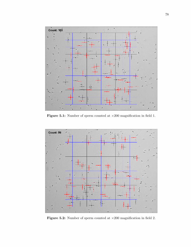
78
Figure 5.1: Number of sperm counted at ⇥200 magnification in field 1.
Figure 5.2: Number of sperm counted at ⇥200 magnification in field 2.
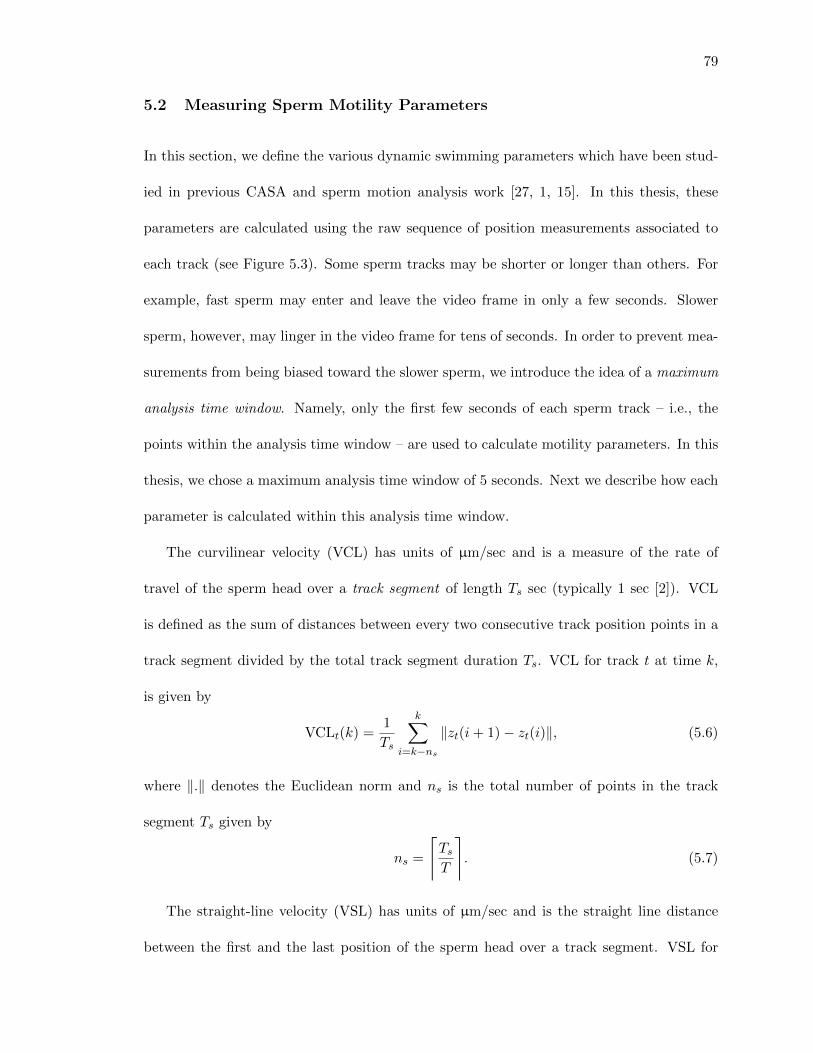
79
5.2 Measuring Sperm Motility Parameters
In this section, we define the various dynamic swimming parameters which have been stud-
ied in previous CASA and sperm motion analysis work [27, 1, 15]. In this thesis, these
parameters are calculated using the raw sequence of position measurements associated to
each track (see Figure 5.3). Some sperm tracks may be shorter or longer than others. For
example, fast sperm may enter and leave the video frame in only a few seconds. Slower
sperm, however, may linger in the video frame for tens of seconds. In order to prevent mea-
surements from being biased toward the slower sperm, we introduce the idea of a maximum
analysis time window. Namely, only the first few seconds of each sperm track – i.e., the
points within the analysis time window – are used to calculate motility parameters. In this
thesis, we chose a maximum analysis time window of 5 seconds. Next we describe how each
parameter is calculated within this analysis time window.
The curvilinear velocity (VCL) has units of µm/sec and is a measure of the rate of
travel of the sperm head over a track segment of length Ts
sec (typically 1 sec [2]). VCL
is defined as the sum of distances between every two consecutive track position points in a
track segment divided by the total track segment duration Ts
. VCL for track t at time k,
is given by
VCLt
(k) =1
Ts
k
X
i=k�ns
kzt
(i+ 1)� zt
(i)k, (5.6)
where k.k denotes the Euclidean norm and ns
is the total number of points in the track
segment Ts
given by
ns
=
&
Ts
T
'
. (5.7)
The straight-line velocity (VSL) has units of µm/sec and is the straight line distance
between the first and the last position of the sperm head over a track segment. VSL for
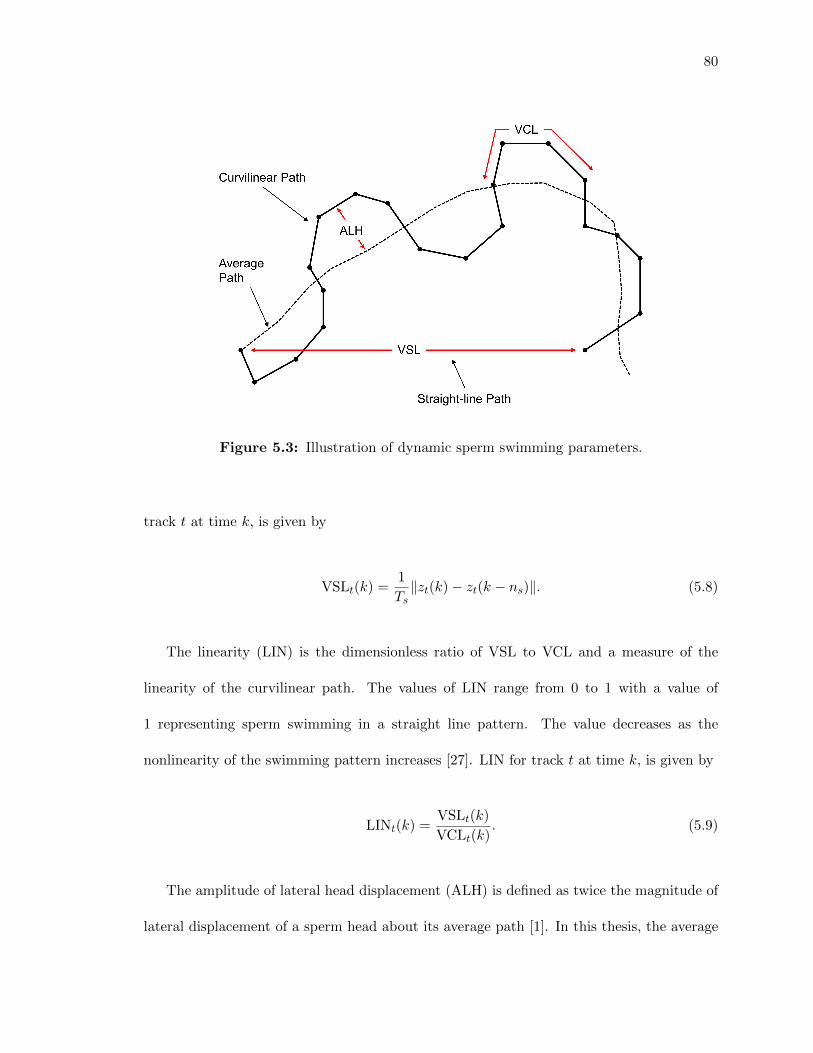
80
Figure 5.3: Illustration of dynamic sperm swimming parameters.
track t at time k, is given by
VSLt
(k) =1
Ts
kzt
(k)� zt
(k � ns
)k. (5.8)
The linearity (LIN) is the dimensionless ratio of VSL to VCL and a measure of the
linearity of the curvilinear path. The values of LIN range from 0 to 1 with a value of
1 representing sperm swimming in a straight line pattern. The value decreases as the
nonlinearity of the swimming pattern increases [27]. LIN for track t at time k, is given by
LINt
(k) =VSL
t
(k)
VCLt
(k). (5.9)
The amplitude of lateral head displacement (ALH) is defined as twice the magnitude of
lateral displacement of a sperm head about its average path [1]. In this thesis, the average
81
path of the sperm is calculated using an na
-point moving average zts
(k) over the track
segment of duration Ts
where na
= 5. The ALH for target track t at time k is then given
by
ALHt
(k) =2
Ts
k
X
i=k�ns
kzt
(i)� zts
(i)k. (5.10)
Now that we have described how these four motility parameters are computed using
sperm track data, in the next chapter we compare the set of motility parameter measure-
ments collected using each of the three tracking algorithms (PDAF, JPDAF and ENN-
JPDAF) applied to simulated sperm trajectories.

82
Chapter 6: Tracking Results Using Simulations
In this chapter, we present and discuss tracking results obtained by applying the PDAF,
JPDAF and ENN-JPDAF algorithms to simulated multi-target scenarios. To compare the
performance of each algorithm objectively, we calculate the optimal subpattern assignment
(OSPA) distance between the set of perfectly known simulated ground truth tracks and the
set of estimated tracks produced by each algorithm. Three simple scenes are generated to
demonstrate the advantages and disadvantages of each algorithm, followed by three real-
istic scenes of swimming sperm simulated at three di↵erent concentrations. In the latter
simulation, the set of motility measurements produced by each algorithm are compared as
a function of increasing concentration.
6.1 Optimal Subpattern Assignment (OSPA) Distance
The performance of a multi-target tracking algorithm is typically assessed using Monte Carlo
simulations whereby the set of estimated tracks produced by the algorithm are compared
to the set of perfectly known ground truth tracks. Such evaluations are often challenging
since the results are highly scenario-dependent and di�cult to quantify in terms of a few
variables [62, 36].
One of the problems that inevitably arises when performing such an evaluation is the
appropriate pairing between estimated and ground truth tracks. In other words: which
estimated track should be compared to which ground truth track? This is illustrated in
Figure 6.1. In the case of a perfect tracker, every estimated track is temporally and spatially

83
Figure 6.1: Four examples of imperfect tracking.
identical to every ground truth track. In practice, (i.e., using an imperfect tracker), an
estimated track may be in the spatial neighborhood of one or more ground truth tracks
(Figure 6.1.A). Furthermore, if an estimated track was initiated late or terminated early
(or both) it may only span a partial segment of a corresponding ground truth track (Figure
6.1.B). A track may initially follow one ground truth track and later swap to another
(Figure 6.1.C). Finally, an estimated track may not exist at all (it was never initiated) for
a corresponding ground truth track (Figure 6.1.D).
In [50], Schuhmacher introduced the optimal subpattern assignment (OSPA) distance
between ground truth and estimated tracks whereby the problem of assigning estimated
tracks to ground truth tracks is solved by casting the problem in terms of an optimal
assignment problem. In [75], Ristic extended the concept of the OSPA distance to labeled
tracks which penalizes an algorithm if track identities are swapped. In this thesis, we use
Ristic’s OSPA distance for labeled tracks to compare multi-target tracking algorithms using
simulations.
The OSPA distance between labeled tracks is a single number that summarizes the per-
formance of a multi-target tracking algorithm due to three sources of tracking error, each

84
expressed as a distance: localization error, labeling error and cardinality error. Although
the OSPA distance is calculated at every time k, it first requires that ground truth tracks
be paired with estimated tracks. This is done by finding the globally optimal permuta-
tion of assignments of ground truth labels to estimated tracks that minimizes the sum of
the distances between pairs of tracks over all time. Once the labeling of tracks has been
completed, the OSPA distance between labeled tracks can be computed.
At time k, the set of q labeled ground truth tracks Xk
is given by
Xk
= {(xk,1
, lx1
), . . . , (xk,q
, lxq
)}, (6.1)
and the set of r labeled estimated tracksYk
produced by the multi-target tracking algorithm
is given by
Yk
= {(yk,1
, ly1
), . . . , (yk,r
, lyr
)}. (6.2)
Here, xk,i
is the position of ground truth track i with label lxi
, i = 1 . . . q and yk,j
is the
position of estimated track j with label lyj
, j = 1 . . . r. The labels associated with a track
do not change with time. For q r, the OSPA distance is given by [50, 75]
do
(Xk
,Yk
) =
"
1
r
min⇡2⇧r
m
X
i=1
�
dc
�
xk,i
, yk,⇡(i)
��
p
+ (r � q)cp!#
1/p
, (6.3)
where xk,i
= (lxi
,xk,i
), yk,⇡(i)
= (ly⇡(i)
,xk,i
), ⇧r
is the set of permutations of length q with
elements taken from {1, 2, . . . , r}, and 1 p 1 is the OSPA order parameter. Note that
for r > q, do
(Xk
,Yk
) = do
(Yk
,Xk
). The cuto↵ distance dc
(x, y) = min(c, d(x, y)) between
the two labeled tracks at time k, with c > 0 being the cuto↵ parameter. The purpose of the
cuto↵ distance is to limit the penalty of assigned tracks which separate to large distances.

85
The base distance between two labeled tracks at time k is defined as
d(x, y) = (d(x,y)p + d(lx, ly)p)1/p , (6.4)
where the localization base distance d(x,y), typically adopted as the p-norm, is given by
d(x,y) = kx� ykp
. (6.5)
The labeling error d(lx, ly) is given by
d(lx, ly) =
8
>
>
>
>
<
>
>
>
>
:
⇠, if lx 6= ly
0, otherwise
(6.6)
where the parameter 0 ⇠ c controls the penalty assigned to the labeling error inter-
preted relative to the localization base distance d(x,y). A value of ⇠ = 0 assigns no penalty
to labeling error and ⇠ = c assigns the maximum penalty. Note that the cardinalities q and
r in Equations (6.1) and (6.2) depend on time k.
6.2 Three Simple Scenarios
This section presents and discusses the result of applying the PDAF, JPDAF and ENN-
JPDAF algorithms to three simple simulated multi-target scenes. Ten Monte Carlo replica-
tions of each scenario were simulated and the mean OSPA distance between labeled tracks
calculated at each time step with p = 1, ⇠ = 25µm, and c = 50µm.
Scenario A: Two Crossing Targets. In this scenario, two targets are separated initially

86
at frame k = 0, cross at frame k = 150, and are separated at frame k = 300. The
starting position and velocity of Target #1 is at x1
(0) = 10 µm, y1
(0) =250 µm and x1
(0)=
28 µm/sec and y1
(0) =-20 µm/sec. The starting position and velocity of Target #2 is
x2
(0) = 10µm, y2
(0) = 50µm and x2
(0) = 28 µm/sec and y2
(0) = 20 µm/sec.
Figure 6.2 depicts the tracking results from one out of the ten Monte Carlo replications
of the scenario using the PDAF. The red lines are the true target trajectories, the blue
lines are the estimated target trajectories, the circles are the validation gates using a gate
threshold of � = 16.2235 drawn at frame k = 20, 150 and 280. From this figure, some of the
drawbacks of the PDAF are readily apparent. Namely, track #2 gets confused the track
#1 and both end up following the same target (Target #2). This causes a new track to be
formed (track #3) after the two targets cross path and begin separating. The initiation of
a new track is seen in the increased value of the mean OSPA distance and mean cardinality
error, depicted in Figure 6.3.
The JPDAF algorithm, in contrast, has no di�culty maintaining track on both targets
before and after they intersect as seen in Figures 6.4 and 6.5. In general, the same is true of
the ENN-JPDAF in Figure 6.6, however it can be seen in Figure 6.7 that the mean OSPA
distance is slightly larger than that of the JPDAF at certain times, indicating that in some
Monte Carlo runs there was a track swap. Based on all three results, JPDAF is the clear
winner here.

87
Figure 6.2: Scenario A using PDAF: ground truth and estimated tracks.
Figure 6.3: Scenario A using PDAF: mean OSPA distance.
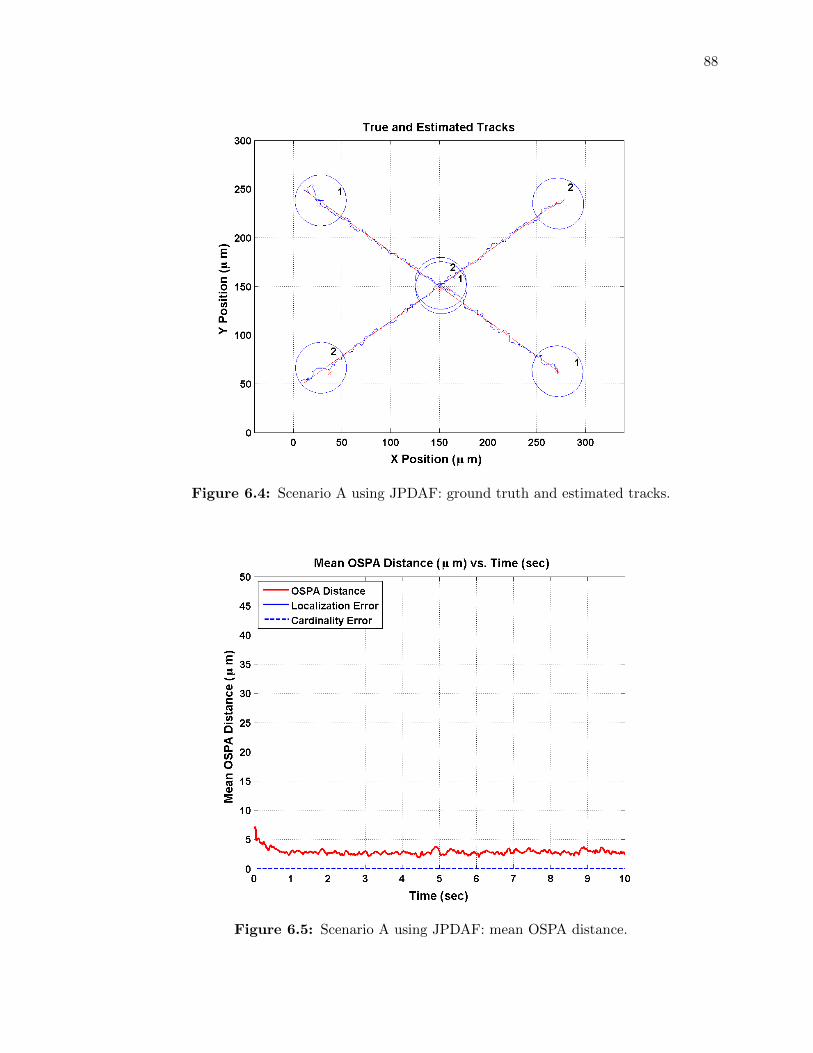
88
Figure 6.4: Scenario A using JPDAF: ground truth and estimated tracks.
Figure 6.5: Scenario A using JPDAF: mean OSPA distance.

89
Figure 6.6: Scenario A using ENN-JPDAF: ground truth and estimated tracks.
Figure 6.7: Scenario A using ENN-JPDAF: mean OSPA distance.

90
Scenario B: Two Targets, Approaching then Separating. In this scenario, two
targets approach each other but move on parallel paths rather than crossing, then eventually
separate. The starting position and velocity of Target #1 is at x1
(0) = 10µm, y1
(0) =
225µm and x1
(0) = 28µm/sec and y1
(0) =-28 µm/sec. The starting position and velocity
of Target #2 is x2
(0) = 10µm, y2
(0) = 75µm and x2
(0) =28 µm/sec and y2
(0) =28 µm/sec.
Between frames k = 70 and k = 81, Target #1 accelerates in the y direction at 2.8 µm/sec2
and Target #2 accelerates in the y direction at -2.8 µm/sec2. Between frames k = 82 and
k = 228, both targets are moving on parallel paths. between frames k = 229 and k = 240,
Target #1 accelerates in the y direction at 2.8 µm/sec2 and Target #2 accelerates in the y
direction at -2.8 µm/sec2.
In this example, the PDAF again performs poorly. From Figure 6.8, one sees that tracks
on Targets #1 and #2 are maintained until they approach one another, where at this time
we see severe track coalescence (a single blue track between the two true target paths). This
is also seen in the mean OSPA distance plot in Figure 6.9 as increased localization error.
Eventually, the PDAF has two tracks following Target #2 and starts a new track (track 3)
to follow true Target #1, which results in an increased cardinality error in the mean OSPA
distance plot.
The JPDAF performs better than the PDAF (see Figure 6.10) in that it never initiated a
new track after the targets separate. However, due to the probability-weighted update step
of the JPDAF it su↵ers from track coalescence which contributes to increased localization
error in the mean OSPA plot 6.11.
The ENN-JPDAF performed the best in this scenario: no new tracks were formed (see
Figure 6.12) and the mean localization error was smaller than that of the JPDAF (see
Figure 6.13). In this case, ENN-JPDAF is the clear winner.

91
Figure 6.8: Scenario B using PDAF: ground truth and estimated tracks.
Figure 6.9: Scenario B using PDAF: mean OSPA distance.

92
Figure 6.10: Scenario B using JPDAF: ground truth and estimated tracks.
Figure 6.11: Scenario B using JPDAF: mean OSPA distance.

93
Figure 6.12: Scenario B using ENN-JPDAF: ground truth and estimated tracks.
Figure 6.13: Scenario B using ENN-JPDAF: mean OSPA distance.

94
Scenario C: Two Parallel Targets and One Crossing Target. In this scenario,
one crossing target intersects the paths of two parallel targets. The starting position and
velocity of Target #1 is at x1
(0) = 10µm, y1
(0) = 175µm and x1
(0) = 28µm/sec and y1
(0) =
0µm/sec. The starting position and velocity of Target #2 is x2
(0) = 10µm, y2
(0) = 125µm
and x2
(0) = 28µm/sec and y2
(0) = 0µm/sec. The starting position and velocity of Target
#3 is x3
(0) = 10µm, y3
(0) = 50µm and x3
(0) = 28µm/sec and y3
(0) = 20µm/sec.
In this example, the PDAF again performs poorly. From Figure 6.14, one sees that
tracks on Targets #1 and #2 are maintained until they are intersected by Target #3. The
PDAF confuses Target #3 with Target #1 and track labels are swapped, and also a new
track is initiated (track 4). Furthermore, tracks 2 and 3 become merged and both follow
Target #2. These tracking errors are seen in the increased mean OSPA distance plot in
Figure 6.15 as increased localization error and cardinality error.
The JPDAF performs better than the PDAF (see Figures 6.16 and 6.17) which tracked
all targets from beginning to end, with some minor increase in the mean OSPA distance
when the tracks approach each other. The results of the ENN-JPDAF are similar (see Fig-
ures 6.18 and 6.19). While the PDAF is the clear loser in this this, the winner is somewhere
between the JPDAF and ENN-JPDAF.
Using the OSPA metric on these three simple scenarios allowed us to objectively com-
pare the PDAF, JPDAF and ENN-JPDAF multi-target tracking algorithms. The plots of
the mean OSPA distance vs. time correlate with tracking errors that can be inferred by
subjective analysis of the tracking results. Animated videos of these three simple scenarios
were generated in which the tracking errors are more easily observed.
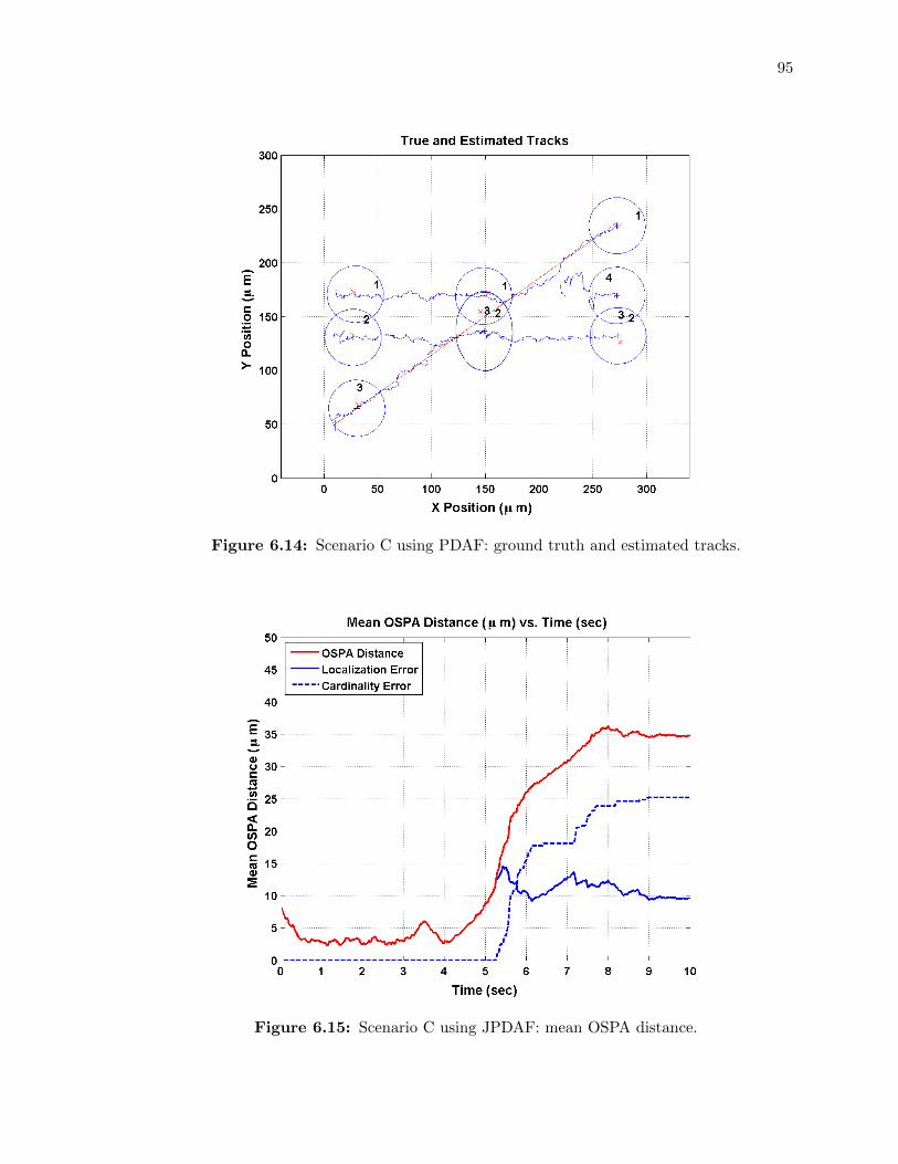
95
Figure 6.14: Scenario C using PDAF: ground truth and estimated tracks.
Figure 6.15: Scenario C using JPDAF: mean OSPA distance.
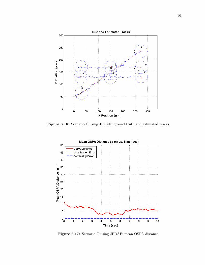
96
Figure 6.16: Scenario C using JPDAF: ground truth and estimated tracks.
Figure 6.17: Scenario C using JPDAF: mean OSPA distance.
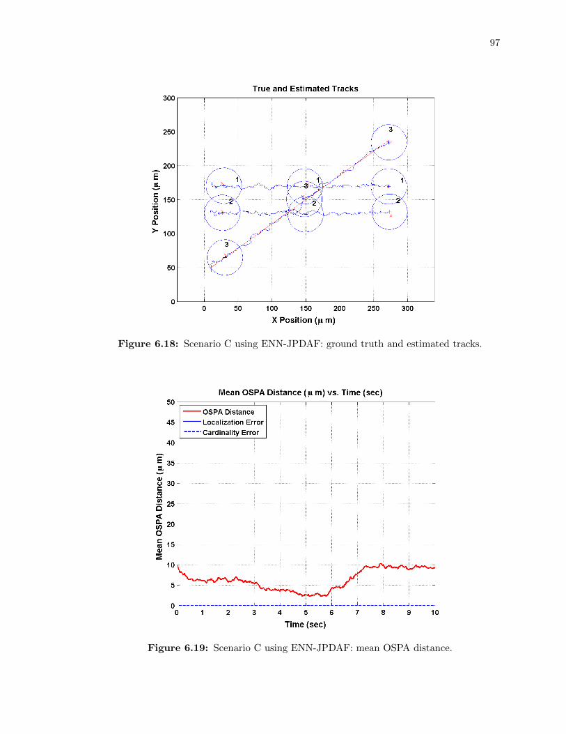
97
Figure 6.18: Scenario C using ENN-JPDAF: ground truth and estimated tracks.
Figure 6.19: Scenario C using ENN-JPDAF: mean OSPA distance.

98
6.3 Simulated Sperm Scenes
In this section, we present and discuss the results of applying the PDAF, JPDAF, and
ENN-JPDAF to simulated scenes, each 10 seconds long, of swimming sperm at three dif-
ferent concentrations: 20, 40 and 60 ⇥106/mL. Assuming a ⇥200 magnification and a
548.5 µm⇥411.4µm field-of-view (the same as our imaging microscope used in our sperm
tracking experiments using real human semen), the three di↵erent simulated concentrations
contained 90, 180 and 270 sperm, respectively.
To simulate realistic sperm swimming motion, we modify a mathematical model of sperm
swimming motion developed in [76] where sperm motion is assumed to obey the nonlinear
equations of motion for a persistent random walk having rotational di↵usion given by
dx
dt= V cos , (6.7)
dy
dt= V sin , (6.8)
and
d
dt=
s
2
⌧p
⇣, (6.9)
where V is the average sperm speed, is the sperm swimming direction angle, ⌧p
is the decay
time constant for directional persistence and ⇣ is zero mean white noise with unity standard
deviation (see Figure 6.20). To make the sperm motion more realistic, a sinusoidal head
wobble motion was added to the simulated paths orthogonal to the instantaneous sperm
swimming direction. The amplitude and frequency of the head wobbling signal were selected
randomly from a normal distribution with parameters typical of human sperm swimming
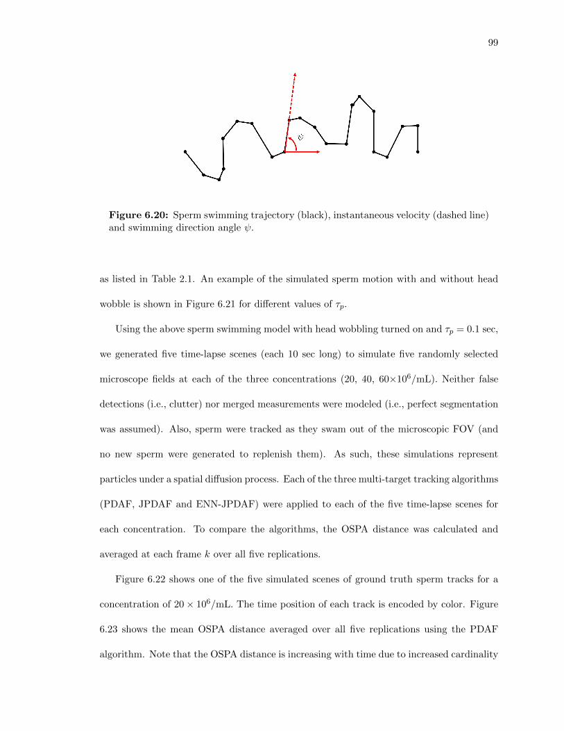
99
Figure 6.20: Sperm swimming trajectory (black), instantaneous velocity (dashed line)and swimming direction angle .
as listed in Table 2.1. An example of the simulated sperm motion with and without head
wobble is shown in Figure 6.21 for di↵erent values of ⌧p
.
Using the above sperm swimming model with head wobbling turned on and ⌧p
= 0.1 sec,
we generated five time-lapse scenes (each 10 sec long) to simulate five randomly selected
microscope fields at each of the three concentrations (20, 40, 60⇥106/mL). Neither false
detections (i.e., clutter) nor merged measurements were modeled (i.e., perfect segmentation
was assumed). Also, sperm were tracked as they swam out of the microscopic FOV (and
no new sperm were generated to replenish them). As such, these simulations represent
particles under a spatial di↵usion process. Each of the three multi-target tracking algorithms
(PDAF, JPDAF and ENN-JPDAF) were applied to each of the five time-lapse scenes for
each concentration. To compare the algorithms, the OSPA distance was calculated and
averaged at each frame k over all five replications.
Figure 6.22 shows one of the five simulated scenes of ground truth sperm tracks for a
concentration of 20⇥ 106/mL. The time position of each track is encoded by color. Figure
6.23 shows the mean OSPA distance averaged over all five replications using the PDAF
algorithm. Note that the OSPA distance is increasing with time due to increased cardinality

100
Figure 6.21: Simulated sperm trajectories at 1/30-sec intervals with and without headwobbling using directional persistence times ⌧
p
= 0.1 sec, 0.01 sec, and 0.001 sec.
error. In other words, multiple tracks are being spawned as sperm swim in close proximity
to each other and the number of estimated tracks is greater than the number of ground
truth tracks. Figure 6.23 shows the mean OSPA distance averaged over all five replications
using the JPDAF algorithm. Note that the mean OSPA distance decreases to a fixed
value as time increases and that there is at least some non-zero cardinality error, indicating
erroneous initiation or deletion of one or more tracks during the five replications. Figure
6.25 shows the mean OSPA distance averaged over all five replications using the ENN-
JPDAF algorithm. Here, the mean OSPA distance remains at a fixed value throughout the
tracking and the cardinality error is zero everywhere.
Figure 6.26 shows one of the five simulated scenes of ground truth sperm tracks for a
concentration of 40⇥106/mL. Figure 6.23 shows the mean OSPA distance averaged over all
five replications using the PDAF algorithm. Compared to the simulation at 20⇥106/mL, the
mean OSPA distance is approximately 5 µm larger over time. Figure 6.28 shows the mean

101
OSPA distance averaged over all five replications using the JPDAF algorithm. Compared to
the simulation at 20⇥106/mL, the peak mean OSPA distance is approximately 2 µm larger
and again there is non-zero cardinality error, indicating erroneous initiation or deletion of
one or more tracks during the five replications. Figure 6.29 shows the mean OSPA distance
averaged over all five replications of the ENN-JPDAF algorithm, which is similar to that of
the JPDAF but with a smaller peak error.
Figure 6.30 shows one of the five simulated scenes of ground truth sperm tracks for a
concentration of 60⇥106/mL. Figure 6.31 shows the mean OSPA distance averaged over all
five replications using the PDAF algorithm. Compared to the simulation at 40⇥ 106/mL,
the mean OSPA distance is again approximately 5 µm larger over time. Figures 6.32 and
6.33 show the mean OSPA distance averaged over all five replications using the JPDAF and
ENN-JPDAF algorithms. Compared to the simulations at 40 ⇥ 106/mL, the peak mean
OSPA distance is slightly larger. By the end of the tracking, the mean OSPA distances
approach similar fixed values. This time however, there is some small non-zero cardinality
error using ENN-JPDAF.
In general, the mean OSPA distance increased with time in all cases for the PDAF. For
the JPDAF and ENN-JPDAF, the mean OSPA distance approached nearly fixed values. To
gain some additional insight into the performance of these algorithms during these tracking
experiments, we measured VCL, VSL, LIN and ALH using each algorithm and calculated
the mean and standard deviation over all five replications. Ground truth and measured
motility parameters for 20, 40 and 60⇥ 106/mL are summarized in Table 6.1, 6.2 and 6.2,
respectively with standard deviations denoted by parentheses. The percent error between
mean value for each parameter is plotted as a function of concentration for each algorithm
in Figure 6.34. Note that for all of the parameters, the ENN-JPDAF has the smallest error

102
compared to ground truth. For this reason, we used the ENN-JPDAF to process time-
lapse images of real sperm collected from a fertility clinic which we now discuss in the next
chapter.

103
Figure 6.22: Simulated 20⇥ 106/mL concentration: ground truth track history.
Figure 6.23: Simulated 20⇥106/mL concentration using PDAF: mean OSPA distance.

104
Figure 6.24: Simulated 20 ⇥ 106/mL concentration using JPDAF: mean OSPA dis-tance.
Figure 6.25: Simulated 20⇥ 106/mL concentration using ENN-JPDAF: mean OSPAdistance.

105
Figure 6.26: Simulated 40⇥ 106/mL concentration using PDAF: track history.
Figure 6.27: Simulated 40⇥106/mL concentration using PDAF: mean OSPA distance.

106
Figure 6.28: Simulated 40 ⇥ 106/mL concentration using JPDAF: mean OSPA dis-tance.
Figure 6.29: Simulated 40⇥ 106/mL concentration using ENN-JPDAF: mean OSPAdistance.
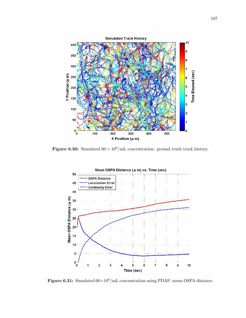
107
Figure 6.30: Simulated 60⇥ 106/mL concentration: ground truth track history.
Figure 6.31: Simulated 60⇥106/mL concentration using PDAF: mean OSPA distance.

108
Figure 6.32: Simulated 60 ⇥ 106/mL concentration using JPDAF: mean OSPA dis-tance.
Figure 6.33: Simulated 60⇥ 106/mL concentration using ENN-JPDAF: mean OSPAdistance.

109
Table 6.1: Motility measurements collected at 20⇥ 106 sperm/mL.
Ground Truth PDAF JPDAF ENN-JPDAF
VCL (µm/sec) 95.56 (19.66) 90.04 (20.61) 94.33 (20.04) 95.70 (19.59)VSL (µm/sec) 45.66 (21.88) 44.14 (21.63) 45.74 (21.91) 45.66 (21.87)LIN 0.47 (0.18) 0.48 (0.19) 0.47 (0.19) 0.47 (0.18)ALH (µm) 3.85 (1.03) 3.59 (1.03) 3.78 (1.04) 3.86 (1.03)
Table 6.2: Motility measurements collected at 40⇥ 106 sperm/mL.
Ground Truth PDAF JPDAF ENN-JPDAF
VCL (µm/sec) 96.06 (20.19) 87.32 (21.22) 94.30 (20.55) 96.37 (20.16)VSL (µm/sec) 46.15 (22.13) 43.92 (21.40) 46.31 (22.10) 46.06 (22.09)LIN 0.47 (0.18) 0.48 (0.19) 0.48 (0.18) 0.47 (0.18)ALH (µm) 3.89 (1.06) 3.46 (1.04) 3.78 (1.04) 3.90 (1.04)
Table 6.3: Motility measurements collected at 60⇥ 106 sperm/mL.
Ground Truth PDAF JPDAF ENN-JPDAF
VCL (µm/sec) 95.96 (20.13) 85.20 (21.42) 93.99 (20.49) 96.59 (20.17)VSL (µm/sec) 46.34 (22.52) 42.41 (22.09) 46.43 (22.55) 46.22 (22.46)LIN 0.47 (0.19) 0.48 (0.19) 0.48 (0.19) 0.47 (0.19)ALH (µm) 3.85 (1.08) 3.34 (1.01) 3.73 (1.03) 3.88 (1.06)

110
Figure 6.34: Percentage error in mean motility parameter measurements.

111
Chapter 7: Tracking Results Using Time-Lapse Images
In this chapter, we discuss the collection and preparation of washed semen samples collected
from five patients by a fertility clinic. Next, we review the semen analysis reports provided
by two technicians for each sample. Finally, we present and discuss the results of applying
the ENN-JPDAF to time-lapse images of these samples.
7.1 Semen Analysis Data from Five Patients
Semen samples were collected from five men at the Penn Fertility Care Center at the Hospital
of the University of Pennsylvania in accordance with university guidelines and allowed to
liquefy at room temperature for at least 30–40 minutes. After mixing the sample well by
repeated aspiration using a pipette, 5 µL of fresh un-washed semen was loaded into each of
the two chambers of a standard MicroCell slide. Next, a second MicroCell slide was loaded
(5 µL per chamber) with washed semen prepared using PureSperm100, a 100% gradient
sterile isotonic salt solution, by centrifugation using for 10 minutes (see Figure 7.1).
A standard manual semen analysis was performed on each of the five un-washed and
washed samples by two separate technicians, referred to here as Tech #1 and Tech #2,
their worksheet data reproduced here in Tables 7.1–7.8. During the analysis, each sample
was kept at 37� C using a thermally regulated microscope stage. Immediately after manual
analysis, each sample was transported to another laboratory (about 5 minutes away) with a
heated microscope stage so that time-lapse images could be recorded. At least five randomly
selected fields of each of the two MicroCell chambers were imaged at ⇥200 magnification

112
Figure 7.1: Sample preparation.
for 8 to 10 minutes.
During the manual analysis, each technician manually measured sperm concentration,
percent motility and percent forward progression in accordance with their local labora-
tory protocol. In addition, the concentration of round cells (if present) were recorded and
whether or not the presence of debris interfered with counting was indicated. The patients
are identified by randomly assigned numbers, given here as 449, 451, 495, 544 and 562.
In Figures 7.2 – 7.7, the measurements from Tech #2 are plotted against those obtained
by Tech #1 for sperm concentration, percent motility, and forward progression for all repli-
113
cate un-washed samples (U1 and U2) and replicate washed samples (W1 and W2). On each
plot, a dashed black line with slope 1 is drawn as a reference and the mean and standard
deviation of the absolute di↵erence between technician measurements (|�|) are given for
each replicate analyzed.
In general, the agreement between the two technicians is greater for the washed sam-
ples than for the un-washed samples. For un-washed semen (Figure 7.2), the mean abso-
lute di↵erence between concentration measurements for U1 was 5.8⇥106/mL with a stan-
dard deviation of 4.44⇥106/mL and for U2 was 2.6⇥106/mL with a standard deviation of
2.88⇥106/mL. For washed semen (Figure 7.3), the mean absolute di↵erence between con-
centration measurements for W1 was 2⇥106/mL with a standard deviation of 1.22⇥106/mL
and for W2 was 1.8⇥106/mL with a standard deviation of 1.3⇥106/mL.
For un-washed semen (Figure 7.4), the mean absolute di↵erence between the measured
percentage of motile sperm for U1 was 7.6 and the standard deviation was 4.04 and for
U2 was 3.8 with a standard deviation of 3.63. For washed semen (Figure 7.5), the mean
absolute di↵erence between the measured percentage of motile sperm for W1 was 1.4 and
the standard deviation was 2.07 and for W2 was 1.4 with a standard deviation of 1.67.
Also, the percent of motile sperm is significantly higher after washing with PureSperm100
(approximately double).
For un-washed semen (Figure 7.6), the mean absolute di↵erence between the measured
percentage of sperm exhibiting forward progression for U1 was 6 with a standard deviation
of 3.61 and for U2 was 3.6 with a standard deviation of 3.05. For washed semen (Figure 7.7),
the mean absolute di↵erence between the measured percentage of sperm exhibiting forward
progression for W1 was 1.2 with a standard deviation 0.837 and for W2 was 1.4 with a
standard deviation of 0.548. Also, the percentage of sperm exhibiting forward progression

114
is significantly higher after washing with PureSperm100 (approximately double)

115
Table 7.1: Semen analysis worksheet: Tech #1 (un-washed semen) chamber U1.
Patient # 449 451 495 544 562
Sperm concentration (⇥10�6/mL) 24 43 26 30 20Round cell concentration (⇥10�6/mL) 7 0 1 1 1Debris interfere with count (Y/N) N N N N NPercent motility (PR + NP) 64% 49% 48% 59% 57%Forward progression (PR) 40% 30% 26% 50% 23%
Table 7.2: Semen analysis worksheet: Tech #1 (un-washed semen) chamber U2.
Patient # 449 451 495 544 562
Sperm concentration (⇥10�6/mL) 21 41 20 35 20Round cell concentration (⇥10�6/mL) 8 1 1 0 1Debris interfere with count (Y/N) N N N N NPercent motility (PR + NP) 70% 49% 39% 48% 51%Forward progression (PR) 35% 32% 23% 43% 21%
Table 7.3: Semen analysis worksheet: Tech #1 (washed semen) chamber W1.
Patient # 449 451 495 544 562
Sperm concentration (⇥10�6/mL) 18 45 4 36 18Round cell concentration (⇥10�6/mL) 0 0 0 0 0Debris interfere with count (Y/N) N N N N NPercent motility (PR + NP) 97% 72% 92% 93% 98%Forward progression (PR) 95% 69% 89% 92% 97%
Table 7.4: Semen analysis worksheet: Tech #1 (washed semen) chamber W2.
Patient # 449 451 495 544 562
Sperm concentration (⇥10�6/mL) 18 43 6 40 25Round cell concentration (⇥10�6/mL) 0 0 0 0 0Debris interfere with count (Y/N) N N N N NPercent motility (PR + NP) 97% 77% 93% 91% 98%Forward progression (PR) 95% 72% 90% 91% 98%
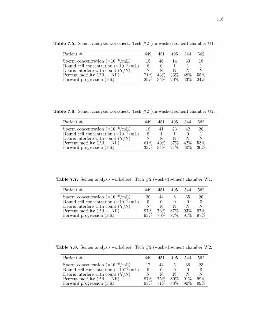
116
Table 7.5: Semen analysis worksheet: Tech #2 (un-washed semen) chamber U1.
Patient # 449 451 495 544 562
Sperm concentration (⇥10�6/mL) 15 46 14 33 18Round cell concentration (⇥10�6/mL) 8 0 1 1 1Debris interfere with count (Y/N) N N N N NPercent motility (PR + NP) 71% 43% 36% 48% 55%Forward progression (PR) 29% 35% 20% 43% 24%
Table 7.6: Semen analysis worksheet: Tech #2 (un-washed semen) chamber U2.
Patient # 449 451 495 544 562
Sperm concentration (⇥10�6/mL) 18 41 23 42 20Round cell concentration (⇥10�6/mL) 8 1 1 0 1Debris interfere with count (Y/N) N N N N NPercent motility (PR + NP) 61% 49% 37% 42% 53%Forward progression (PR) 33% 34% 21% 40% 30%
Table 7.7: Semen analysis worksheet: Tech #2 (washed semen) chamber W1.
Patient # 449 451 495 544 562
Sperm concentration (⇥10�6/mL) 20 44 8 35 20Round cell concentration (⇥10�6/mL) 0 0 0 0 0Debris interfere with count (Y/N) N N N N NPercent motility (PR + NP) 97% 73% 87% 93% 97%Forward progression (PR) 93% 70% 87% 91% 97%
Table 7.8: Semen analysis worksheet: Tech #2 (washed semen) chamber W2.
Patient # 449 451 495 544 562
Sperm concentration (⇥10�6/mL) 17 44 5 36 23Round cell concentration (⇥10�6/mL) 0 0 0 0 0Debris interfere with count (Y/N) N N N N NPercent motility (PR + NP) 97% 75% 89% 91% 99%Forward progression (PR) 93% 71% 88% 90% 99%

117
Figure 7.2: Five patients: sperm concentration (un-washed semen).
Figure 7.3: Five patients: sperm concentration (washed semen).

118
Figure 7.4: Five patients: percent motility (un-washed semen).
Figure 7.5: Five patients: percent motility (washed semen).

119
Figure 7.6: Five patients: percent forward progression (un-washed semen).
Figure 7.7: Five patients: percent forward progression (washed semen).

120
7.2 Tracking and Motility Analysis of Sperm in Time-Lapse Images
In this section, we present and describe the results of applying the ENN-JPDAF algorithm
to videos of sperm samples from the five patients. Image segmentation, multi-sperm tracking
and motility parameter measurement were done automatically with no human intervention.
To assess the reproducibility of our algorithm, we analyzed video clips (each 30 sec long) for
three randomly selected microscopic fields (denoted here by the letters A, B and C). Only
motile sperm (i.e., sperm having VCL > 30 µm/sec [15]) and sperm having a total track
length > 3 sec were analyzed. This was done to exclude drifting debris, spurious tracks
and sperm which orbit the edges of the microscope field-of-view from biasing the analysis.
Motility parameters VCL, VSL, LIN and ALH were measured over the first 5 sec of each
sperm track using a 1 sec moving average window.
The tracking results are visualized in several ways. First, we show a snapshot of the
tracks produced by the multi-target tracking algorithm superimposed on a randomly chosen
video frame. Next, we show the 30 sec track histories obtained of each sperm tracked for
each field examined. These pictures show the swimming paths of the sperm observed in
each patient sample. The motility measurements collected for each field are then displayed
in two ways: (1) a scatterplot of VCL and VSL measurements and a scatterplot of LIN and
ALH measurements, with points colored by their relative density and (2) separate box and
whisker plots for VCL, VSL, LIN and ALH. In the box and whisker plots, the bottom and
top edges of each box are the 25-th and 75-th percentiles (i.e., the first and third quartiles),
the central red line mark is the median (the third quartile), and the whiskers extend to 1.5
times the di↵erence between the third and first quartiles and the outliers are drawn as red
crosses.

121
Figure 7.8: Patient No. 449, snapshot of multi-target tracking for chamber W1.
Patient No. 449. Figure 7.8 shows sperm tracks superimposed on a snapshot from the
video clip of field A. Three di↵erent microscopic fields were chosen randomly within chamber
W1 of the MicroCell and imaged for 30 sec each. The 30 sec track histories obtained by the
multi-sperm tracking algorithm for each field are depicted in Figure 7.9. The time of each
point on the plotted tracks is encoded by its color. A total of 162, 111 and 201 tracks were
analyzed in fields A, B, and C, respectively. Figure 7.10 and Figure 7.11 shows scatterplots
of the motility measurements collected for each field. The distribution of the VCL, VSL,
LIN, and ALH measurements collected for each field are summarized using box and whisker
plots in Figures 7.12, 7.13, 7.14, and 7.15. From these plots, the median value of VCL
is approximately 85 µm/sec, the median value of VSL is approximately 50 µm/sec, the
median value of LIN is approximately 0.55, and the median value of ALH is approximately
5 µm/sec.

122
0 100 200 300 400 5000
50
100
150
200
250
300
350
400
X (µm)
Y (µ
m)
Patient 449, Field A (162 Tracks Analyzed)
Tim
e El
apse
d (s
ec)
0
5
10
15
20
25
30
Figure 7.9: Patient No. 449, 30 sec track histories for fields A, B, and C.
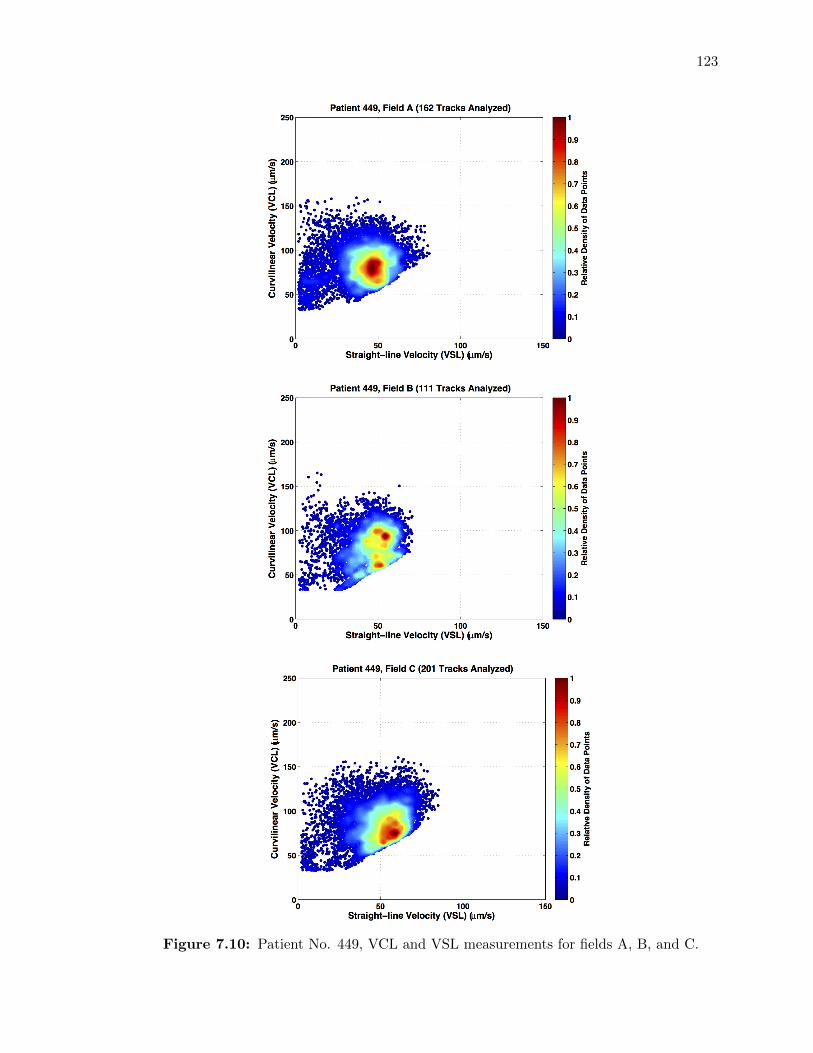
123
Figure 7.10: Patient No. 449, VCL and VSL measurements for fields A, B, and C.
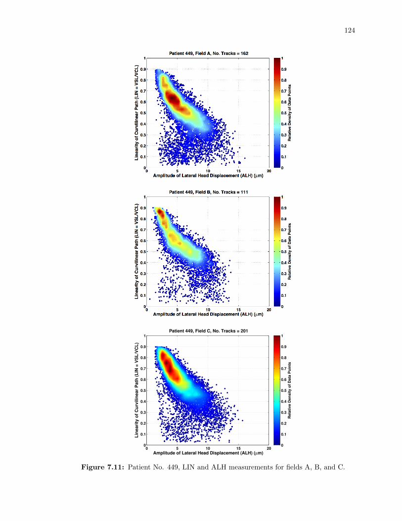
124
0 5 10 15 200
0.1
0.2
0.3
0.4
0.5
0.6
0.7
0.8
0.9
1
Amplitude of Lateral Head Displacement (ALH) (µm)
Lin
eari
ty o
f C
urv
ilin
ear
Path
(L
IN =
VS
L/V
CL
)
Patient 449, Field C, No. Tracks = 201
Rela
tive D
en
sit
y o
f D
ata
Po
ints
0
0.1
0.2
0.3
0.4
0.5
0.6
0.7
0.8
0.9
1
Figure 7.11: Patient No. 449, LIN and ALH measurements for fields A, B, and C.
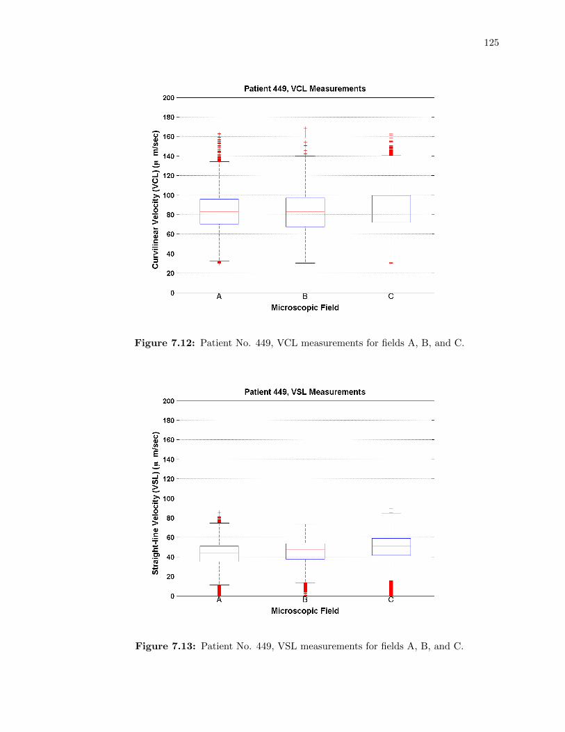
125
Figure 7.12: Patient No. 449, VCL measurements for fields A, B, and C.
Figure 7.13: Patient No. 449, VSL measurements for fields A, B, and C.

126
Figure 7.14: Patient No. 449, LIN measurements for fields A, B, and C.
Figure 7.15: Patient No. 449, ALH measurements for fields A, B, and C.

127
Figure 7.16: Patient No. 451, snapshot of multi-target tracking for chamber W1.
Patient No. 451. Figure 7.16 shows sperm tracks superimposed on a snapshot from the
video clip of field A. Three di↵erent microscopic fields were chosen randomly within chamber
W1 of the MicroCell and imaged for 30 sec each. The 30 sec track histories obtained by the
multi-sperm tracking algorithm for each field are depicted in Figure 7.17. The time of each
point on the plotted tracks is encoded by its color. A total of 510, 470 and 271 tracks were
analyzed in fields A, B, and C, respectively. Figure 7.18 and Figure 7.19 show scatterplots
of the motility measurements collected for each field. The distribution of the VCL, VSL,
LIN, and ALH measurements collected for each field are summarized using box and whisker
plots in Figures 7.20, 7.21, 7.22, and 7.23. From these plots, the median value of VCL
is approximately 65 µm/sec, the median value of VSL is approximately 35 µm/sec, the
median value of LIN is approximately 0.6, and the median value of ALH is approximately
3.8 µm/sec.

128
Figure 7.17: Patient No. 451, 30 sec track histories for fields A, B, and C.
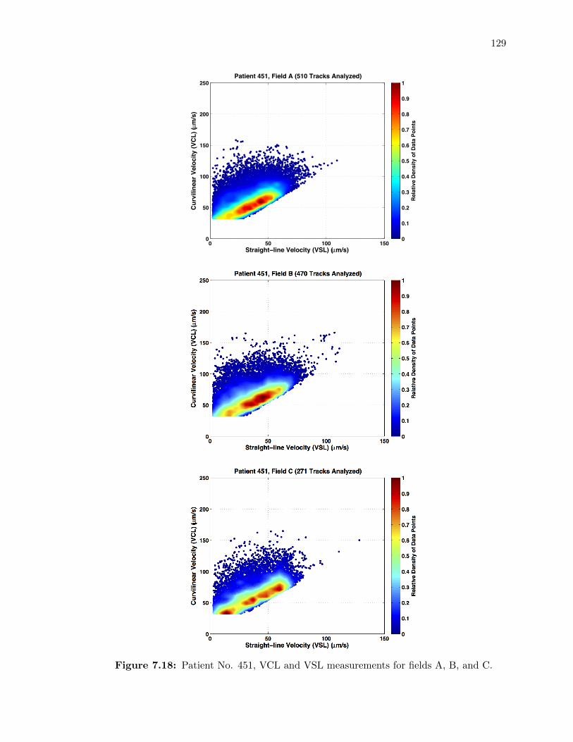
129
0 50 100 1500
50
100
150
200
250
Straight−line Velocity (VSL) (µm/s)
Curv
iline
ar V
eloc
ity (V
CL) (µm
/s)
Patient 451, Field A (510 Tracks Analyzed)
Rela
tive
Dens
ity o
f Dat
a Po
ints
0
0.1
0.2
0.3
0.4
0.5
0.6
0.7
0.8
0.9
1
Figure 7.18: Patient No. 451, VCL and VSL measurements for fields A, B, and C.
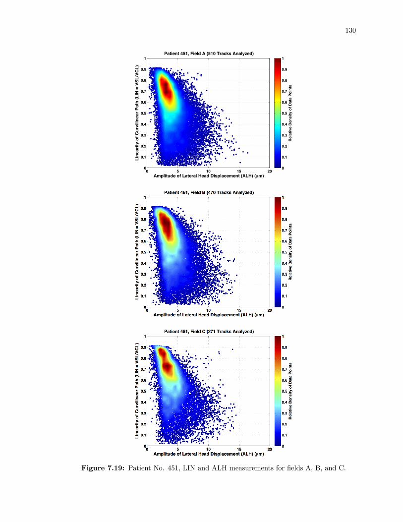
130
0 5 10 15 200
0.1
0.2
0.3
0.4
0.5
0.6
0.7
0.8
0.9
1
Amplitude of Lateral Head Displacement (ALH) (µm)
Line
arity
of C
urvi
linea
r Pat
h (L
IN =
VSL
/VC
L)
Patient 451, Field A (510 Tracks Analyzed)
Rel
ativ
e D
ensi
ty o
f Dat
a Po
ints
0
0.1
0.2
0.3
0.4
0.5
0.6
0.7
0.8
0.9
1
Figure 7.19: Patient No. 451, LIN and ALH measurements for fields A, B, and C.

131
Figure 7.20: Patient No. 451, VCL measurements for fields A, B, and C.
Figure 7.21: Patient No. 451, VSL measurements for fields A, B, and C.

132
Figure 7.22: Patient No. 451, LIN measurements for fields A, B, and C.
Figure 7.23: Patient No. 451, ALH measurements for fields A, B, and C.

133
Figure 7.24: Patient No. 495, snapshot of multi-target tracking for chamber W1.
Patient No. 495. Figure 7.24 shows sperm tracks superimposed on a snapshot from the
video clip of field A. Three di↵erent microscopic fields were chosen randomly within chamber
W1 of the MicroCell and imaged for 30 sec each. The 30 sec track histories obtained by
the multi-sperm tracking algorithm for each field are depicted in Figure 7.25. The time of
each point on the plotted tracks is encoded by its color. A total of 17, 8 and 7 tracks were
analyzed in fields A, B, and C, respectively. Figure 7.26 and Figure 7.27 show scatterplots
of the motility measurements collected for each field. The distribution of the VCL, VSL,
LIN, and ALH measurements collected for each field are summarized using box and whisker
plots in Figures 7.28, 7.29, 7.30, and 7.31. Due to the limited number of sperm available to
analyze for this patient, the median values of VCL, VSL, LIN and ALH are seen to fluctuate
across fields.

134
Figure 7.25: Patient No. 495, 30 sec track histories for fields A, B, and C.

135
Figure 7.26: Patient No. 495, VCL and VSL measurements for fields A, B, and C.

136
0 5 10 15 200
0.1
0.2
0.3
0.4
0.5
0.6
0.7
0.8
0.9
1
Amplitude of Lateral Head Displacement (ALH) (µm)
Line
arity
of C
urvi
linea
r Pat
h (L
IN =
VSL
/VC
L)
Patient 495, Field A (17 Tracks Analyzed)
Rel
ativ
e D
ensi
ty o
f Dat
a Po
ints
0
0.1
0.2
0.3
0.4
0.5
0.6
0.7
0.8
0.9
1
Figure 7.27: Patient No. 495, LIN and ALH measurements for fields A, B, and C.
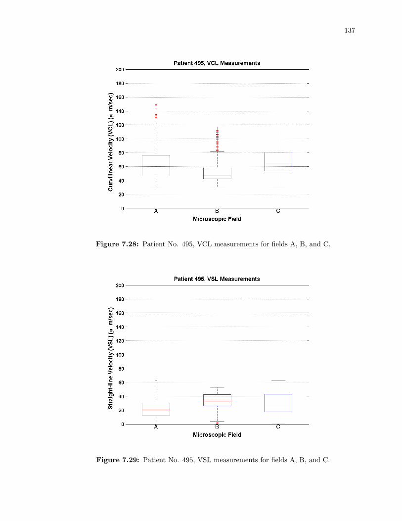
137
Figure 7.28: Patient No. 495, VCL measurements for fields A, B, and C.
Figure 7.29: Patient No. 495, VSL measurements for fields A, B, and C.

138
Figure 7.30: Patient No. 495, LIN measurements for fields A, B, and C.
Figure 7.31: Patient No. 495, LIN measurements for fields A, B, and C.

139
Figure 7.32: Patient No. 544, snapshot of multi-target tracking for chamber W1.
Patient No. 544. Figure 7.32 shows sperm tracks superimposed on a snapshot from the
video clip of field A. Three di↵erent microscopic fields were chosen randomly within chamber
W1 of the MicroCell and imaged for 30 sec each. The 30 sec track histories obtained by the
multi-sperm tracking algorithm for each field are depicted in Figure 7.33. The time of each
point on the plotted tracks is encoded by its color. A total of 199, 172 and 191 tracks were
analyzed in fields A, B, and C, respectively. Figure 7.34 and Figure 7.35 show scatterplots
of the motility measurements collected for each field. The distribution of the VCL, VSL,
LIN, and ALH measurements collected for each field are summarized using box and whisker
plots in Figures 7.36, 7.37, 7.38, and 7.39. From these plots, the median value of VCL
is approximately 60 µm/sec, the median value of VSL is approximately 35 µm/sec, the
median value of LIN is approximately 0.55, and the median value of ALH is approximately
4 µm/sec.

140
Figure 7.33: Patient No. 495, 30 sec track histories for fields A, B, and C.
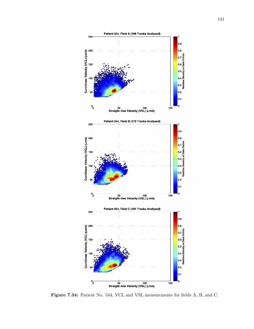
141
Figure 7.34: Patient No. 544, VCL and VSL measurements for fields A, B, and C.

142
Figure 7.35: Patient No. 544, VCL and VSL measurements for fields A, B, and C.

143
Figure 7.36: Patient No. 544, VCL measurements for fields A, B, and C.
Figure 7.37: Patient No. 544, VSL measurements for fields A, B, and C.

144
Figure 7.38: Patient No. 544, LIN measurements for fields A, B, and C.
Figure 7.39: Patient No. 544, ALH measurements for fields A, B, and C.

145
Figure 7.40: Patient No. 562, snapshot of multi-target tracking for chamber W1.
Patient No. 562. Figure 7.40 shows sperm tracks superimposed on a snapshot from the
video clip of field A. Three di↵erent microscopic fields were chosen randomly within chamber
W1 of the MicroCell and imaged for 30 sec each. The 30 sec track histories obtained by the
multi-sperm tracking algorithm for each field are depicted in Figure 7.41. The time of each
point on the plotted tracks is encoded by its color. A total of 34, 58 and 53 tracks were
analyzed in fields A, B, and C, respectively. Figure 7.42 and Figure 7.43 show scatterplots
of the motility measurements collected for each field. The distribution of the VCL, VSL,
LIN, and ALH measurements collected for each field are summarized using box and whisker
plots in Figures 7.44, 7.45, 7.46, and 7.47. From these plots, the median value of VCL
is approximately 60 µm/sec, the median value of VSL is approximately 35 µm/sec, the
median value of LIN is approximately 0.75, and the median value of ALH is approximately
3 µm/sec.

146
Figure 7.41: Patient No. 562, 30 sec track histories for fields A, B, and C.
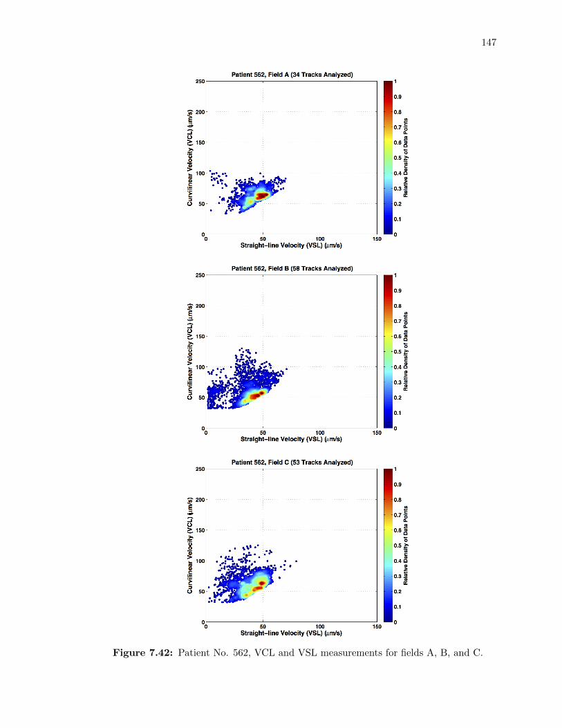
147
Figure 7.42: Patient No. 562, VCL and VSL measurements for fields A, B, and C.

148
Figure 7.43: Patient No. 562, LIN and ALH measurements for fields A, B, and C.

149
Figure 7.44: Patient No. 562, VCL measurements for fields A, B, and C.
Figure 7.45: Patient No. 562, VSL measurements for fields A, B, and C.
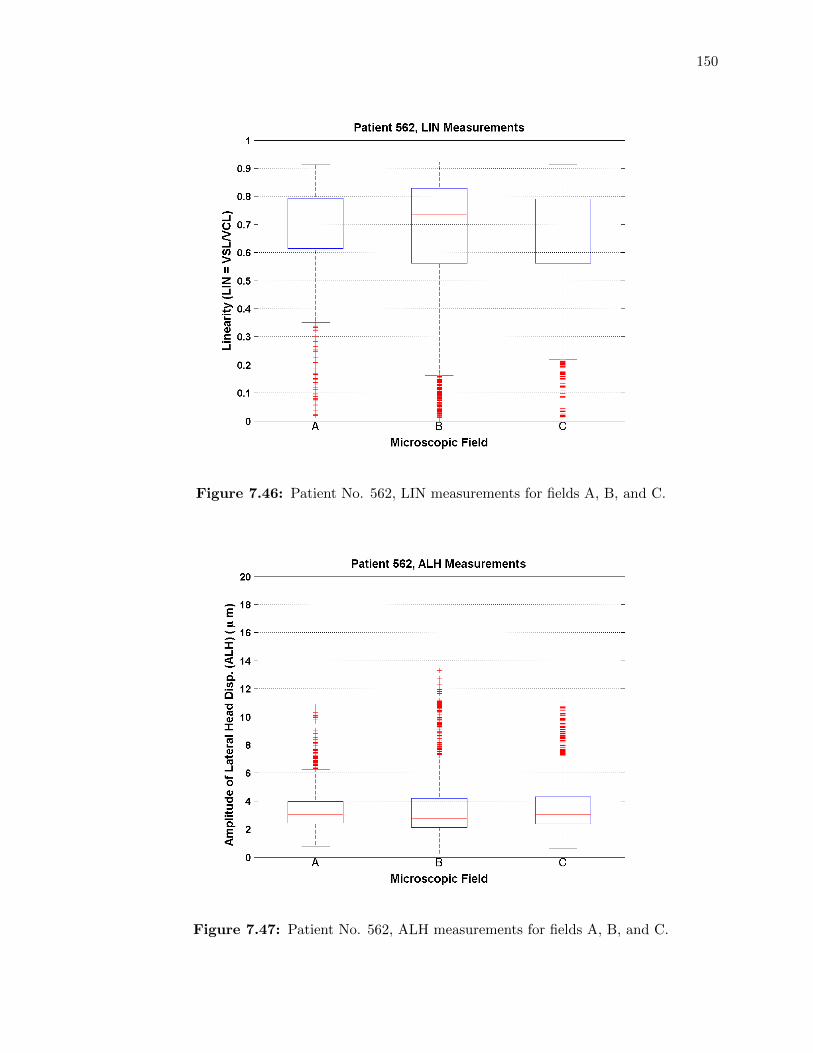
150
Figure 7.46: Patient No. 562, LIN measurements for fields A, B, and C.
Figure 7.47: Patient No. 562, ALH measurements for fields A, B, and C.

151
Chapter 8: Concluding Remarks
In this thesis, we presented a robust automatic multi-sperm tracking algorithm that can
measure dynamic sperm motility parameters over time in pre-recorded time-lapse images.
We evaluated three multi-target tracking algorithms: the probabilistic data association fil-
ter (PDAF), the joint probabilistic data association filter (JPDAF) and the exact nearest
neighbor extension to the JPDAF (ENN-JPDAF). Based on simulation results, we selected
the ENN-JPDA to apply to time-lapse images of human sperm obtained from a fertility
clinic. Simultaneous tracking and motility analysis of hundreds of sperms was demon-
strated. Combined analysis, testing and simulation support the use of probabilistic data
association techniques robust automatic multi-sperm tracking. This method could provide
fertility specialists with new data visualizations and interpretations previously impossible
with existing laboratory protocols. In future work, we will explore methods for dealing with
merged measurements and examine time-lapse images captured at higher frame rates (60
fps).
152
Bibliography
[1] WHO, Laboratory Manual for the Examination and Processing of Human Semen, 5thEdition. World Health Organization, 2010.
[2] D. Mortimer, Practical Laboratory Andrology. Oxford University Press, USA, 1994.
[3] C. Opinion, “Diagnostic evaluation of the infertile male,” Fertility and Sterility, vol. 98,no. 2, pp. 294–301, 2012.
[4] J. Liu, C. Leung, Z. Lu, and Y. Sun, “Quantitative analysis of locomotive behavior ofhuman sperm head and tail,” Biomedical Engineering, IEEE Transactions on, vol. 60,no. 2, pp. 390–396, 2013.
[5] C. Schleh and A.-L. Leoni, “How to optimize the benefits of computer assisted spermanalysis in experimental toxicology,” Journal of Occupational Medicine and Toxicology,vol. 8, no. 6, 2013.
[6] A. P. Chong, C. A. Walters, and S. A. Weinrieb, “The neglected laboratory test: thesemen analysis,” Journal of Andrology, vol. 4, no. 4, pp. 280–282, 1983.
[7] C. H. Yueng, T. G. Cooper, and E. Nieschlag, “A technique for standardization andquality control of subjective sperm motility assessments in semen analysis,” Fertilityand Sterility, vol. 67, no. 6, pp. 1156–1158, 1997.
[8] S. A. Rothmann and A. A. Reese, “Semen analysis: the test techs love to hate,” MedicalLaboratory Observer, 2007.
[9] K. A. Brooks, “How reliable are results from the semen analysis?,” Fertility and Steril-ity, vol. 82, no. 1, pp. 41–44, 1983.
[10] S. T. Mortimer, “CASA: Practical aspects,” Journal of Andrology, vol. 21, no. 4,pp. 515–524, 2000.
[11] R. P. Amann and D. F. Katz, “Andrology lab corner: Reflections on CASA after 25years,” Journal of Andrology, vol. 25, no. 3, pp. 317–325, 2004.
[12] R. J. Sherins, “Clinical use and misuse of automated semen analysis,” Annals of theNew York Academy of Sciences, vol. 637, no. 1, pp. 424–435, 1991.
[13] W. contributors, “Epididymis,” Wikipedia, The Free Encylcopedia, 2013. Online, ac-cessed 20 April 2014.
[14] “Spermatogenesis,” The Turek Clinic, http://www.theturekclinic.com; accessed April6th, 2014.
[15] T.-W. Su, L. Xue, and A. Ozcan, “High-throughput lensfree 3D tracking of hu-man sperms reveals rare statistics of helical trajectories,” Proceedings of the NationalAcademy of Sciences, vol. 109, no. 40, pp. 16018–16022, 2012.

153
[16] E. A. Ga↵ney, H. Gadelha, D. J. Smith, J. R. Blake, and J. C. Kirkman-Brown, “Mam-malian sperm motility: observation and theory,” Annual Review of Fluid Mechanics,vol. 43, pp. 501–528, 2011.
[17] D. J. Lamb, “Semen analysis in 21st century medicine: the need for sperm functiontesting,” Asian Journal of Andrology, vol. 12, no. 6, pp. 64–70, 2010.
[18] Vitrolife, “Microcell User Manual 1.3,” 2012.
[19] R. O. Davis and D. F. Katz, “Standardization and comparability of casa instruments,”Journal of Andrology, vol. 13, January/February 1992.
[20] D. H. Owen and D. F. Katz, “Sampling factors influencing accuracy of sperm kinematicanalysis,” Journal of Andrology, vol. 14, May/June 1993.
[21] X. Albe, J. Auger, S. Margules, and J. C. Bisconte, “Measurement of spermatozoalmotility over prolonged periods of time using image analysis,” Computers and Biomed-ical Research, vol. 21, no. 3, pp. 276–288, 1988.
[22] L. Robertson, D. P. Wolf, and J. S. Tash, “Temporal changes in motility parame-ters related to acrosomal status: identification and characterization of populations ofhyperactivated human sperm,” Biology of Reproduction, vol. 39, no. 4, pp. 797–805,1988.
[23] F. Mazzilli, T. Rossi, M. Delfino, and I. Nofroni, “Accuracy of computer-assisted semenanalysis in prefreeze and post-thaw specimens with high and low sperm counts andmotility,” Andrologia, vol. 31, no. 4, pp. 187–194, 1999.
[24] R. S. Sidhu, R. K. Sharma, J.-C. Lee, and A. Agarwal, “Accuracy of computer-assistedsemen analysis in prefreeze and post-thaw specimens with high and low sperm countsand motility,” Urology, vol. 51, no. 2, pp. 306–312, 1998.
[25] T. G. Cooper and C.-H. Yeung, “Computer-aided evaluation of assessment of grade aspermatozoa by experienced technicians,” Fertility and Sterility, vol. 85, no. 1, pp. 220–224, 2006.
[26] C. H. Yueng and E. Nieschlag, “Performance and comparison of CASA systemsequipped with di↵erent phase-contrast optics,” Journal of Andrology, vol. 14, no. 3,pp. 1939–4640, 1993.
[27] S. O. Mack, D. P. Wolf, and J. S. Tash, “Quantitation of specific parameters of motilityin large numbers of human sperm by digital image processing,” Biology of Reproduction,vol. 38, no. 2, pp. 270–281, 1988.
[28] D. Katz, R. Davis, B. Delandmeter, and J. Overstreet, “Real-time analysis of spermmotion using automatic video image digitization,” Computer Methods and Programsin Biomedicine, vol. 21, no. 3, pp. 173–182, 1985.
[29] S. T. Mortimer and M. A. Swan, “E↵ect of image sampling frequency on established andsmoothing-indepdenent kinematic values of capacitating human spermatozoa,” HumanReproduction, vol. 14, no. 4, pp. 997–1004, 1999.

154
[30] H. F. M. Broekhujse and B. Gadella, “Do CASA systems satisfy consumers demands?a critical analysis.,” Reproduction in Domestic Animals, vol. 46, no. 2, pp. 49–51, 2011.
[31] A. Gelb, Applied Optimal Estimation. The MIT Press, 1974.
[32] Y. Bar-Shalom and P. Fortmann, Tracking and data association. San Diego, CA, USA:Academic Press, 1988.
[33] S. Blackman and R. Popoli, Design and Analysis of Modern Tracking Systems. ArtechHouse Radar Library, 1999.
[34] A. Yilmaz, O. Javed, and M. Shah, “Object tracking: a survey,” ACM ComputingSurveys, vol. 38, no. 4, 2006.
[35] E. Meijering, “Cell segmentation: 50 years down the road,” IEEE Signal ProcessingMagazine, vol. 29, pp. 140–145, September 2012.
[36] N. Chenouard and et. al., “Objective comparison of particle tracking methods,” NatureMethods, vol. 11, pp. 281–289, 2014.
[37] M. J. Saxton, “Single-particle tracking: connecting the dots,” Nature Methods, vol. 5,pp. 671–672, August 2008.
[38] C. Rasmussen and G. D. Hager, “Probabilistic data association methods for trackingcomplex visual objects,” Pattern Analysis and Machine Intelligence, IEEE Transac-tions on, vol. 23, no. 6, pp. 560–576, 2001.
[39] D. B. Reid, “An algorithm for tracking multiple targets,” IEEE Transactions on Au-tomatic Control, vol. 24, no. 6, pp. 843–854, 1979.
[40] Y. Bar-Shalom, F. Daum, and J. Huang, “The probabilistic data association filter,”IEEE Control Systems Magazine, pp. 82–100, December 2009.
[41] T. E. Fortmann, Y. Bar-Shalom, and M. Sche↵e, “Sonar tracking of multiple targetsusing joint probabilistic data association,” Oceanic Engineering, IEEE Journal of,vol. 8, no. 3, pp. 174–184, 1983.
[42] T. Kirubarajan, Y. Bar-Shalom, and K. R. Pattipati, “Multiassignment for tracking alarge number of overlapping objects,” IEEE Transactions on Aerospace and ElectronicSystems, vol. 37, no. 1, pp. 2–21, 2001.
[43] S. T. Young, W. L. Tzeng, Y. L. Kuo, M. L. Hsiao, and S. R. Chiang, “Real-time tracingof spermatozoa,” Engineering in Medicine and Biology Magazine, IEEE, vol. 15, no. 6,pp. 117–120, 1996.
[44] B. Beresford-Smith and D. V. Helden, “Applications of radar tracking algorithms tomotion analysis in biomedical images,” Image Processing, Proceedings of the IEEEInternational Conference on, no. 1, pp. 411–415, 1994.
[45] M. J. Tomlinson and K. Poole, “Validation of a novel computer-assisted sperm analysis(casa) system using multitarget-tracking algorithms,” Fertility and Sterility, vol. 93,no. 6, pp. 1911–1920, 2010.

155
[46] Z. Khan, T. Balch, and F. Dellaert, “An mcmc-based particle filter for tracking multipleinteracting targets,” Lecture Notes in Computer Science, vol. 3024, pp. 279–290, 2004.
[47] T.-W. Su, A. Erlinger, D. Tseng, and A. Ozcan, “Compact and light-weight auto-mated semen analysis platform using lensfree on-chip microscopy,” Annals of Chem-istry, vol. 82, pp. 8307–8312, 2010.
[48] T.-W. Su, I. Choi, J. Feng, K. Huang, E. McLeod, and A. Ozcan, “Sperm trajectoriesform chiral ribbons,” Scientific Reports, Nature, vol. 3, no. 1664, 2013.
[49] J. C. Crocker and D. G. Grier, “Methods of digital video microscopy for colloidalstudies,” Journal of Colloid and Interface Science, vol. 179, pp. 298–310, 1996.
[50] D. Schuhmacher, B.-T. Vo, , and B.-N. Vo, “A consistent metric for performanceevaluation of multi-object filters,” Signal Processing, IEEE Transactions on, vol. 56,no. 8, pp. 3447–3457, 2008.
[51] Wikipedia Contributors, “Page: Antonie van Leeuwenhoek,” Wikipedia, The Free En-cyclopedia.
[52] N. Otsu, “A threshold selection method from gray-level histograms,” IEEE Transac-tions on Systems, Man, and Cybernetics, vol. 9, pp. 62–66, January 1979.
[53] W. Pratt, Digital Image Processing, 4th Edition. Wiley-Interscience, 2007.
[54] B. Friedland, “Optimum steady-state position and velocity estimation using noisy sam-pled position data,” IEEE Transactions on Aerospace and Electronic Systems, vol. 9,no. 6, pp. 907–911, 1973.
[55] P. R. Kalata, “The tracking index: A generalized parameter for ↵-� and ↵-�-� targettrackers,” Aerospace and Electronic Systems, IEEE Transactions on, vol. 20, no. 2,pp. 174–182, 1984.
[56] B. Friedland, “On the properties of reduced-order kalman filters,” Proceedings of the28th Conference on Decision and Control, pp. 1601–1604, December 1987.
[57] Y. Bar-Shalom, X. Li, and T. Kirubarajan, Estimation with Applications to Trackingand Navigation. Wiley-Interscience, 2001.
[58] S. Blackman, Multiple-target Tracking with Radar Applications. Artech House, 1986.
[59] W. D. Blair, “Design of nearly constant velocity track filters for tracking maneuveringtargets,” Information Fusion, 2008 11th International Conference on, pp. 1–7, 2008.
[60] W. D. Blair, “Design of nearly constant velocity track filters for brief maneuvers,”Information Fusion (FUSION), 2011 Proceedings of the 14th International Conferenceon, pp. 1–8, 2011.
[61] G. Portmann, J. Moore, and W. Bath, “Separated covariance filtering,” IEEE Inter-national Radar Conference, pp. 456–460, 1990.
[62] R. J. Fitzgerald, “Development of practical PDA logic for multitarget tracking bymicroprocessor,” Proceedings of the American Control Conference, pp. 889–898, June1986.
156
[63] W. Blair and Y. Bar-Shalom, “Tracking maneuvering targets with multiple sensors:does more data always mean better estimates?,” IEEE Transactions on Aerospace andElectronic Systems, vol. 32, pp. 450–456, January 1996.
[64] W. Blair and Y. Bar-Shalom, “Maneuver-driven ↵-� and ↵-�-� tracking filters,” IEEETransactions on Aerospace and Electronic Systems, vol. 31, no. 1, pp. 341–357, 1995.
[65] B. M. Friedrich, I. H. Riedel-Kruse, J. Howard, and F. Julicher, “High-precision track-ing of sperm swimming fine structure provides strong test of resistive force theory,”The Journal of Experimental Biology, vol. 213, pp. 1226–1234, 2010.
[66] Y. Bar-Shalom, “Tracking methods in a multitarget environment,” Automatic Control,IEEE Transactions on, vol. 23, no. 4, pp. 618–626, 1978.
[67] I. J. Cox, “On finding ranked assignments with application to multitarget tracking andmotion correspondence,” Aerospace and Electronic Systems, IEEE Transactions on,vol. 31, no. 1, pp. 486–489, 1995.
[68] K. Romeo, D. F. Crouse, Y. Bar-Shalom, and P. Willett, “A fast coalescence-avoidingJPDAF,” Signal and Data Processing of Small Targets, vol. 8393, 2012.
[69] S. Challa, M. R. Morelande, D. Musicki, and R. J. Evans, Fundamentals of ObjectTracking. Cambridge University Press, 2011.
[70] F. Bourgeois and J.-C. Lassalle, “An extension of the munkres algorithm to the assign-ment problem to rectangular matrices,” Communications of the ACM, vol. 14, no. 12,pp. 802–804, 1971.
[71] K. G. Murty, “An algorithm for ranking all the assignments in order of increasing cost,”Operations Research, vol. 16, no. 3, pp. 682–687, 1968.
[72] J. J. Stein and S. S. Blackman, “Generalized correlation of multi-target track data,”IEEE Transactions on Aerospace and Electronic Systems, vol. 11, pp. 1207–1217,November 1975.
[73] Y. Bar-Shalom, S. S. Blackman, and R. J. Fitzgerald, “Dimensionless score function formultiple hypothesis tracking,” Aerospace and Electronic Systems, IEEE Transactionson, vol. 43, no. 1, pp. 392–400, 2007.
[74] J. K. Uhlmann, “Algorithms for multiple-target tracking,” American Scientist, vol. 80,pp. 128–143, 1992.
[75] B. Ristic, B.-N. Vo, D. Clark, , and B.-T. Vo, “A metric for performance evaluation ofmulti-target tracking algorithms,” Signal Processing, IEEE Transactions on, vol. 59,no. 7, pp. 3452–3457, 2011.
[76] L. Armon, S. R. Caplan, M. Eisenbach, and B. M. Friedrich, “Testing human spermchemotaxis: how to detect biased motion in population assays,” PLoS ONE, vol. 7,no. 3, 2012.

157
Appendix A: MATLAB code for Murty’s method
Below is the MATLAB listing implementing Murty’s method which was developed for this
thesis.
1 function [SOLUTIONS] = murtys best(P0, S0, V0, N)2 % 1. Find the best solution S0 to P0.3 % [S0, V0] = munkres(P0);45 % 2. Initialize the list of problem / solution pairs with P0, S0, V06 P{1} = P0; S{1} = S0; V(1) = V0;78 % 3. Clear the list of solutions to be returned9 SOLUTIONS = [];
1011 % 4. For k = 1 to N (or until the list of P/S pairs is empty)12 for k = 1 : N1314 % 4.1 Find the solution with the best (minimum) value V15 best idx = find(V == min(V), 1);1617 % If its not empty18 if ˜isempty(best idx)19 P BEST = P{best idx};20 S BEST = S{best idx};21 V BEST = V(best idx);2223 % 4.2 Remove <P,S> from the list of P/S pairs24 P{best idx} = [];25 P(cellfun(@(P) isempty(P), P)) = [];26 S{best idx} = [];27 S(cellfun (@(S) isempty(S), S)) = [];28 V(best idx) = [];2930 % 4.3 Add S to the list of solutions to be returned31 SOLUTIONS{end+1} = S BEST;3233 % 4.4 For each assignment in S34 [ i , j ] = find(S BEST);35 for n = 1:length(i)3637 % 4.4.1 Let P’ = P
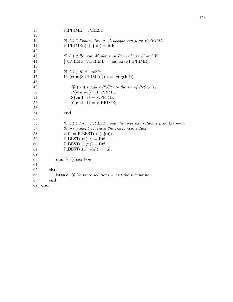
158
38 P PRIME = P BEST;3940 % 4.4.2 Remove this n�th assignment from P PRIME41 P PRIME(i(n), j(n)) = Inf;4243 % 4.4.3 Re�run Munkres on P’ to obtain S’ and V’44 [S PRIME, V PRIME] = munkres(P PRIME);4546 % 4.4.4 If S’ exists47 if (sum(S PRIME(:)) == length(i))4849 % 4.4.4.1 Add <P’,S’> to the set of P/S pairs50 P{end+1} = P PRIME;51 S{end+1} = S PRIME;52 V(end+1) = V PRIME;5354 end5556 % 4.4.5 From P BEST, clear the rows and columns from the n�th57 % assignment but leave the assignment intact58 a ij = P BEST(i(n), j(n));59 P BEST(i(n), :) = Inf;60 P BEST(:, j(n)) = Inf;61 P BEST(i(n), j(n)) = a ij;6263 end % // end loop6465 else66 break % No more solutions � exit the subroutine67 end68 end
159
Vita
Leonardo Francesco Urbano was born in New York City, New York. He received his B.S.
and M.S. in Electrical Engineering from the Department of Electrical and Computer Engi-
neering, Drexel University, Philadelphia, in 2005 and 2007, respectively. He joined the Data
Fusion Laboratory at Drexel University in 2002 under the supervision of Dr. Moshe Kam.
His research has spanned a variety of areas in computer engineering and control theory
such as a banana and strawberry. He has also been a teaching assistant in the Department
from 2004 to 2006. His teaching responsibilities include lecture, recitation, help session, and
quiz/homework assignment and grading.
He has served as Secretary of the IEEE Philadelphia Section since 2013. He is a member
of the IEEE and the American Society of Andrology.