Time-lapse monitoring of localized changes within ...

TIME-LAPSE MONITORING OF LOCALIZED

CHANGES WITHIN HETEROGENEOUS

MEDIA WITH SCATTERED WAVES

by

Kanu Chinaemerem

c� Copyright by Kanu Chinaemerem, 2014

All Rights Reserved

A thesis submitted to the Faculty and the Board of Trustees of the Colorado School

of Mines in partial fulfillment of the requirements for the degree of Doctor of Philosophy

(Geophysics).

Golden, Colorado

Date

Signed:Kanu Chinaemerem

Signed:Dr. Roel SniederThesis Advisor

Golden, Colorado

Date

Signed:Dr. Terry Young

Professor and HeadDepartment of Geophysics

ii

ABSTRACT

Time-lapse monitoring of geological and mechanical media has been the focus of various

studies over the past four decades because of the information that the inferred changes within

the medium provides insight into the dynamic characteristics of the medium. Time-lapse

changes within a medium can be used to characterize the temporal evolution of the medium,

evaluate the forces driving the changes within the medium and make predictions on the future

state of the monitored medium. The detectability of the changes within a material depends

on the characteristics of the change to be imaged, the sensitivity of the monitoring data to

the change, and the time-lapse monitoring parameters such as the monitoring source-receiver

array and the spectral content of the monitoring waves. Various time-lapse monitoring tools

have been used to monitor changes within media ranging from the earth’s surface to tumors

within the human body. These monitoring tools include the use of 4D active surveys were

an imprint of the change within the medium is extracted from the time-lapse surveys and

the use of interferometric techniques that use singly or multiply scattered waves.

My major goal in this study is to image and localize changes present within a scattering

medium using time-lapse multiply scattered waves generated within the monitored medium.

The changes to be imaged are generally localized in space. This work is an extension of coda

wave interferometry. Coda wave interferometry focuses on the identification and extraction

of average velocity change occurring within a scattering medium. Due to the non-linear char-

acteristics of multiply scattered waves and limited information of the origin of the multiply

scattered waves, coda wave interferometry resolves the average velocity change within the

scattering medium with no or limited indication of the location of the change. In this study,

I demonstrate that time-lapse changes can be imaged and localized within scattering media

using travel-time changes or decorrelation estimated from the time-lapse coda waves. The

imaging algorithm is defined to invert for the location and magnitude of changes within both

iii

statistically homogeneous and statistically heterogeneous scattering media. The imaging of

the localized change requires an appropriate computation of the sensitivity of the scattered

waves to the monitored change.

I develop a novel approach to compute the sensitivity kernel needed to image localized

changes present within a scattering medium. I compute the sensitivity kernel, using an

a-priori scattering model that has similar statistical properties as the actual medium, by

computing the intensity of the scattered waves generated at both the source and the receiver

locations. This approach of the kernel computation allows one to compute the sensitiv-

ity kernel for any heterogeneous scattering medium with a prescribed boundary condition.

Generating the kernel with the a priori model prevents one from invoking a homogeneity

assumption of the scattering model.

I apply the imaging algorithm on both numerical and laboratory experiments. The

numerical experiment provides an opportunity to evaluate the resolution of the monitored

change for each coda lapse time. In the laboratory experiment, I accurately resolve the

change induced within two concrete blocks due to localize stress and heat changes. I also

monitored velocity changes present within the subsurface beneath the Eastern section of the

Basin and Range Province, Western US. Time-lapse monitoring with coda waves, generated

with repeating active sources, over a period of four months suggests of the presence of a

maximum velocity change of approximately 0.2% with the Eastern section of the Basin and

Range Province. This observed velocity change are likely induced by the deformation within

the Basin and Range Province.

iv

TABLE OF CONTENTS

ABSTRACT . . . . . . . . . . . . . . . . . . . . . . . . . . . . . . . . . . . . . . . . . iii

LIST OF FIGURES . . . . . . . . . . . . . . . . . . . . . . . . . . . . . . . . . . . . . . x

LIST OF TABLES . . . . . . . . . . . . . . . . . . . . . . . . . . . . . . . . . . . . . . xxi

ACKNOWLEDGMENTS . . . . . . . . . . . . . . . . . . . . . . . . . . . . . . . . . xxii

DEDICATION . . . . . . . . . . . . . . . . . . . . . . . . . . . . . . . . . . . . . . . xxv

CHAPTER 1 INTRODUCTION . . . . . . . . . . . . . . . . . . . . . . . . . . . . . . . 1

CHAPTER 2 ESTIMATION OF VELOCITY CHANGE USING REPEATINGEARTHQUAKES WITH DIFFERENT LOCATIONS AND FOCALMECHANISMS . . . . . . . . . . . . . . . . . . . . . . . . . . . . . . . . 6

2.1 Abstract . . . . . . . . . . . . . . . . . . . . . . . . . . . . . . . . . . . . . . . . 6

2.2 Introduction . . . . . . . . . . . . . . . . . . . . . . . . . . . . . . . . . . . . . . 6

2.3 Mathematical Consideration . . . . . . . . . . . . . . . . . . . . . . . . . . . . . 8

2.4 Numerical Validation . . . . . . . . . . . . . . . . . . . . . . . . . . . . . . . . 11

2.4.1 Data processing . . . . . . . . . . . . . . . . . . . . . . . . . . . . . . . 15

2.4.2 E↵ect of perturbation of source properties on the estimated velocitychange . . . . . . . . . . . . . . . . . . . . . . . . . . . . . . . . . . . . 16

2.4.3 Limiting regimes of the estimations . . . . . . . . . . . . . . . . . . . . 20

2.5 Discussion and Conclusion . . . . . . . . . . . . . . . . . . . . . . . . . . . . . 25

2.6 Acknowledgments . . . . . . . . . . . . . . . . . . . . . . . . . . . . . . . . . . 28

CHAPTER 3 A COMPARISON OF THREE METHODS FOR ESTIMATINGVELOCITY CHANGES BETWEEN TIME-LAPSE MICROSEISMICSIGNALS . . . . . . . . . . . . . . . . . . . . . . . . . . . . . . . . . . . 29

v

3.1 Abstract . . . . . . . . . . . . . . . . . . . . . . . . . . . . . . . . . . . . . . . 29

3.2 Introduction . . . . . . . . . . . . . . . . . . . . . . . . . . . . . . . . . . . . . 29

3.3 Methods . . . . . . . . . . . . . . . . . . . . . . . . . . . . . . . . . . . . . . . 30

3.3.1 Windowed cross-correlation . . . . . . . . . . . . . . . . . . . . . . . . 31

3.3.2 Stretching method . . . . . . . . . . . . . . . . . . . . . . . . . . . . . 33

3.3.3 Smooth dynamic time warping . . . . . . . . . . . . . . . . . . . . . . . 35

3.4 Real microseismic signals . . . . . . . . . . . . . . . . . . . . . . . . . . . . . . 36

3.5 Monitoring with downhole arrays . . . . . . . . . . . . . . . . . . . . . . . . . 41

3.6 Conclusion . . . . . . . . . . . . . . . . . . . . . . . . . . . . . . . . . . . . . . 44


CHAPTER 4 NUMERICAL COMPUTATION OF THE SENSITIVITY KERNELFOR TIME-LAPSE MONITORING WITH MULTIPLYSCATTERED ACOUSTIC WAVES . . . . . . . . . . . . . . . . . . . . 47

4.1 Abstract . . . . . . . . . . . . . . . . . . . . . . . . . . . . . . . . . . . . . . . 47

4.2 Introduction . . . . . . . . . . . . . . . . . . . . . . . . . . . . . . . . . . . . . 47

4.3 Sensitivity Kernel . . . . . . . . . . . . . . . . . . . . . . . . . . . . . . . . . . 50

4.4 Numerical computation . . . . . . . . . . . . . . . . . . . . . . . . . . . . . . . 51

4.4.1 Numerical vs. analytical computation . . . . . . . . . . . . . . . . . . . 53

4.4.2 Scattering Velocity models . . . . . . . . . . . . . . . . . . . . . . . . . 58

4.4.3 Topography-induced Scattering . . . . . . . . . . . . . . . . . . . . . . 65

4.5 Discussion and Conclusion . . . . . . . . . . . . . . . . . . . . . . . . . . . . . 72


CHAPTER 5 NUMERICAL COMPUTATION OF THE SENSITIVITY KERNELFOR TIME-LAPSE MONITORING WITH MULTIPLYSCATTERED ELASTIC WAVES . . . . . . . . . . . . . . . . . . . . . 77

vi

5.1 Abstract . . . . . . . . . . . . . . . . . . . . . . . . . . . . . . . . . . . . . . . 77

5.2 Introduction . . . . . . . . . . . . . . . . . . . . . . . . . . . . . . . . . . . . . 77

5.3 Mean travel-time change in an elastic coda interferometry . . . . . . . . . . . . 79

5.4 Mean travel-time change with multiply scattered elastic intensity . . . . . . . . 80

5.5 Random isotropic scattering model . . . . . . . . . . . . . . . . . . . . . . . . 83

5.5.1 Sensitivity to perturbations in P-wave velocity . . . . . . . . . . . . . . 87

5.5.2 Sensitivity to perturbations in S-wave velocity . . . . . . . . . . . . . . 89

5.6 Heterogeneous scattering model with free-surface . . . . . . . . . . . . . . . . 92

5.6.1 Sensitivity to perturbations in P-wave velocity . . . . . . . . . . . . . . 95

5.6.2 Sensitivity to perturbations in S-wave velocity . . . . . . . . . . . . . . 99

5.7 Discussion and Conclusion . . . . . . . . . . . . . . . . . . . . . . . . . . . . 100

5.8 Acknowledgments . . . . . . . . . . . . . . . . . . . . . . . . . . . . . . . . . 101

CHAPTER 6 TIME-LAPSE IMAGING OF LOCALIZED WEAK CHANGESWITH MULTIPLY SCATTERED WAVES: NUMERICALEXPERIMENT . . . . . . . . . . . . . . . . . . . . . . . . . . . . . . 102

6.1 Abstract . . . . . . . . . . . . . . . . . . . . . . . . . . . . . . . . . . . . . . 102

6.2 Introduction . . . . . . . . . . . . . . . . . . . . . . . . . . . . . . . . . . . . 102

6.3 Theory . . . . . . . . . . . . . . . . . . . . . . . . . . . . . . . . . . . . . . . 104

6.4 Model setup: . . . . . . . . . . . . . . . . . . . . . . . . . . . . . . . . . . . 106

6.5 Model and Data resolution . . . . . . . . . . . . . . . . . . . . . . . . . . . . 108

6.6 Time-lapse inversion . . . . . . . . . . . . . . . . . . . . . . . . . . . . . . . 114

6.7 Conclusions . . . . . . . . . . . . . . . . . . . . . . . . . . . . . . . . . . . . 115


vii

CHAPTER 7 TIME-LAPSE IMAGING OF LOCALIZED WEAK CHANGESWITH MULTIPLY SCATTERED WAVES: LABORATORYEXPERIMENT . . . . . . . . . . . . . . . . . . . . . . . . . . . . . . 118

7.1 Abstract . . . . . . . . . . . . . . . . . . . . . . . . . . . . . . . . . . . . . . 118

7.2 Introduction . . . . . . . . . . . . . . . . . . . . . . . . . . . . . . . . . . . . 118

7.3 Theory . . . . . . . . . . . . . . . . . . . . . . . . . . . . . . . . . . . . . . . 119

7.4 Laboratory experiment in a concrete block . . . . . . . . . . . . . . . . . . . 121

7.5 Data analysis . . . . . . . . . . . . . . . . . . . . . . . . . . . . . . . . . . . 130

7.6 Time-lapse inversion . . . . . . . . . . . . . . . . . . . . . . . . . . . . . . . 133

7.7 Conclusion . . . . . . . . . . . . . . . . . . . . . . . . . . . . . . . . . . . . . 137

CHAPTER 8 TIME-LAPSE MONITORING ACROSS UTAH AND EASTERNSECTION OF BASIN AND RANGE . . . . . . . . . . . . . . . . . . 138

8.1 Abstract . . . . . . . . . . . . . . . . . . . . . . . . . . . . . . . . . . . . . . 138

8.2 Introduction . . . . . . . . . . . . . . . . . . . . . . . . . . . . . . . . . . . . 138

8.3 Data processing . . . . . . . . . . . . . . . . . . . . . . . . . . . . . . . . . . 141

8.4 Time-lapse velocity change . . . . . . . . . . . . . . . . . . . . . . . . . . . . 145

8.4.1 Spatial distribution of velocity change . . . . . . . . . . . . . . . . . . 146

8.4.2 Coda time window analysis of h✏i . . . . . . . . . . . . . . . . . . . . 146

8.4.3 Parameter Estimation . . . . . . . . . . . . . . . . . . . . . . . . . . 152

8.5 Causes for the velocity changes . . . . . . . . . . . . . . . . . . . . . . . . . 156

8.5.1 Seasonal loading . . . . . . . . . . . . . . . . . . . . . . . . . . . . . 156

8.5.2 Local seismicity . . . . . . . . . . . . . . . . . . . . . . . . . . . . . . 161

8.6 Discussion and Conclusions . . . . . . . . . . . . . . . . . . . . . . . . . . . 163


viii

CHAPTER 9 CONCLUSION AND FUTURE WORK . . . . . . . . . . . . . . . . . 170

REFERENCES CITED . . . . . . . . . . . . . . . . . . . . . . . . . . . . . . . . . . 173

APPENDIX A - THE TIME PERTURBATION DUE TO A PERTURBEDSOURCE . . . . . . . . . . . . . . . . . . . . . . . . . . . . . . . . . 183

APPENDIX B - VARIANCE OF THE TIME PERTURBATION . . . . . . . . . . . 185

APPENDIX C - ERROR ESTIMATION . . . . . . . . . . . . . . . . . . . . . . . . . 186

APPENDIX D - COMPARATIVE TIME SHIFT BETWEEN CHANGES INVELOCITY AND SOURCE LOCATION . . . . . . . . . . . . . . . 188

APPENDIX E - ANALYTICAL APPROXIMATION OF THE MODEL OFPACHECO AND SNIEDER [70] . . . . . . . . . . . . . . . . . . . . 190

ix

LIST OF FIGURES

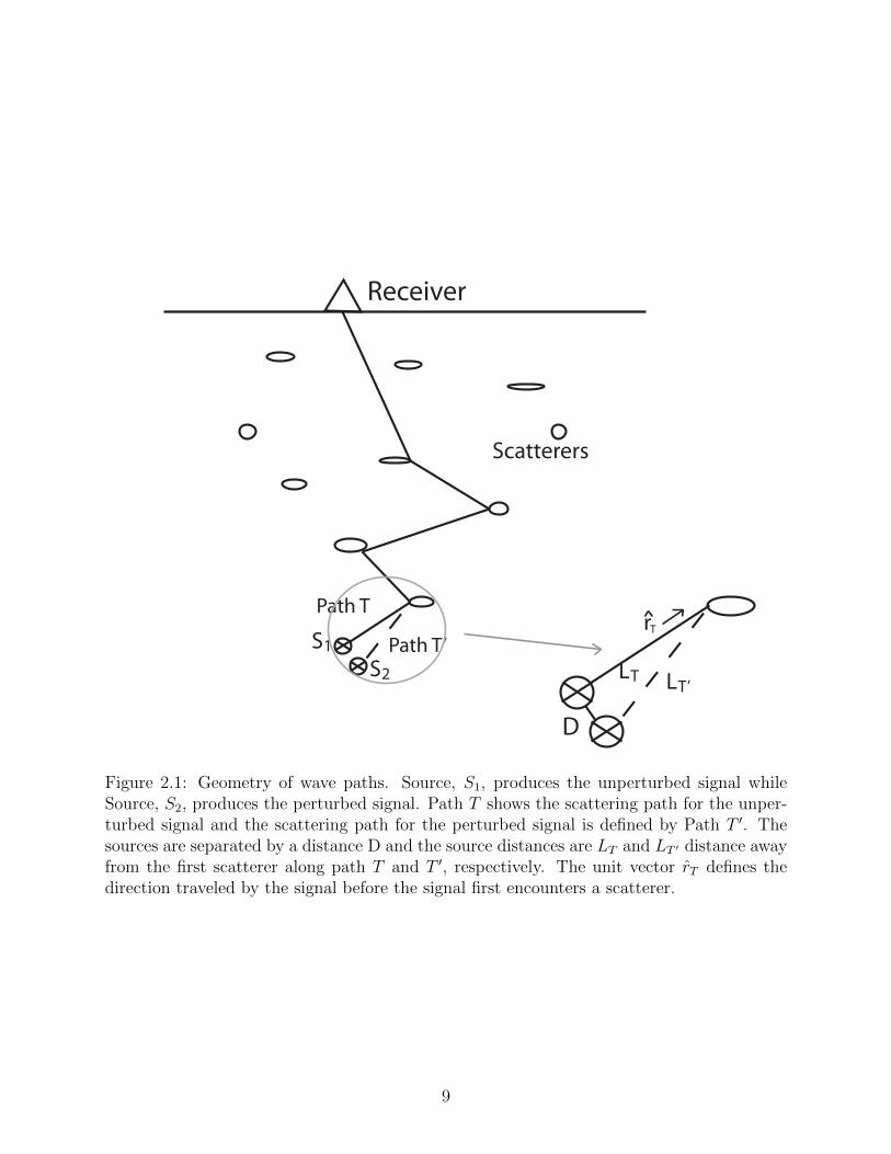
Figure 2.1 Geometry of wave paths. Source, S1, produces the unperturbed signalwhile Source, S2, produces the perturbed signal. Path T shows thescattering path for the unperturbed signal and the scattering path forthe perturbed signal is defined by Path T 0. The sources are separatedby a distance D and the source distances are L

T

and LT

0 distance awayfrom the first scatterer along path T and T 0, respectively. The unitvector r

T

defines the direction traveled by the signal before the signalfirst encounters a scatterer. . . . . . . . . . . . . . . . . . . . . . . . . . . . 9

Figure 2.2 The experiment geometry of the numerical simulation. The receivers(squares) are surrounding the point scatterers (black dots). The sourceis positioned in the origin (cross). All perturbations of the sourcelocation is done from this position. The stations marked (NW, NE, E,SE, and SW) are used in the presentation of results in Figure 2.7 andFigure 2.8. . . . . . . . . . . . . . . . . . . . . . . . . . . . . . . . . . . . 12

Figure 2.3 Recorded seismic signals at station E (Figure 2.2), the reference signal(red line) and the time-lapse signal (black line) with 0.4% relativevelocity change (I), the time-lapse signal (black line) with 0.14�

d

sourcedisplacement (II), and the time-lapse signal (black line) with 20o sourceangle perturbations (III). Inset A shows the late coda while inset Bshows the first arrivals of the two signals. The black bold line is thetime window used for data processing. Time 0 is the source rupture time. . 14

Figure 2.4 The objective function R(✏) (solid line) as a function of the stretchfactor ✏. The objective function is minimum for ✏ = 0.4%, whichcorresponds to the time-lapse velocity change. The correspondingmaximum correlation of the stretch factors is given by the dash lines. . . 17

Figure 2.5 Estimated relative velocity change for model velocity change of h �VV0i =

0.1% (blue), h �VV0i = 0.2% (red), h �V

V0i = 0.3% (black), and h �V

V0i = 0.4%

(green). The receiver numbers are counted counter-clockwise from theW station in Figure 2.2. . . . . . . . . . . . . . . . . . . . . . . . . . . . 18

x

Figure 2.6 Estimated relative velocity change due to perturbation in the sourcelocation and the source radiation. A. The estimated velocity change forperturbed source location (divided by the dominant wavelength; insetin the top right) and B. The estimated velocity change caused bychanges in source radiation angles (inset in the top right). The value of⇣ is given by equation 2.15. The receiver numbers are countedcounter-clockwise from the W station in Figure 2.2. . . . . . . . . . . . . 19

Figure 2.7 Estimated relative velocity change after a 0.1% velocity change andvarious source location perturbations (Table 2.1). The shift in thesource locations are divided by the dominant wavelength �

d

of therecorded signals. For values of the source location shift greater than�d

/4, we have incorrect estimates for the velocity change due to thedistortion of the perturbed signal. Stations SW, SE, NE, and NWpositions are given in Figure 2.2. The red line indicates the model(accurate) velocity change. . . . . . . . . . . . . . . . . . . . . . . . . . . 22

Figure 2.8 E↵ect of source angle perturbation on estimated velocity change. A.The estimated relative velocity changes are from a 0.1% model velocitychange (Red line) and various source radiation perturbations(Table 2.2). B. The decorrelation of the doublets, due to source angleperturbations, measured by maximum cross-correlation values. StationsSW, SE, NE, and NW positions are given in Figure 2.2. . . . . . . . . . . 24

Figure 2.9 Source radiation pattern of the modeled earthquake sources before andafter simultaneous perturbation of the source angles (strike ��, rake�� and dip ��) of 20 degree each. . . . . . . . . . . . . . . . . . . . . . . 26

Figure 3.1 Synthetic time-lapse signals (a) and recorded microseismic time lapsesignals (b). The blue curve is the baseline signal and the red curve isthe time-lapse signal. . . . . . . . . . . . . . . . . . . . . . . . . . . . . . 30

Figure 3.2 The stability of the windowed cross-correlation method for time shiftestimation. The time shifts are estimated within time windows whosewidths 2t

w

are relative to the dominant period T of the signal: 2tw

=37.5T (a), 2t

w

= 75T (b), and 2tw

= 112.5T (c), where T = 0.033 s. . . . 32

Figure 3.3 The stability of the windowed stretching method for relative velocitychange estimation. The relative velocity changes are estimated withintime windows whose widths are relative to the dominant period T ofthe signal: 37.5T (a), 75T (b), and 112.5T (c), where T = 0.033 s. Thered line shows the exact relative velocity change. . . . . . . . . . . . . . . 34

xi

Figure 3.4 Time shifts and relative velocity changes estimated via SDTW. Thetime shifts (a) and the relative velocity changes (b) are computed fromthe synthetic time-lapse signals shown in Figure 3.1a. We compare theexact velocity change (red) to the estimated relative velocity changes(blue) (b). . . . . . . . . . . . . . . . . . . . . . . . . . . . . . . . . . . . 37

Figure 3.5 Time shifts computed from the unfiltered time-lapse microseismicsignals (a) using windowed cross-correlation (b), the windowedstretching method (c), and SDTW (d). . . . . . . . . . . . . . . . . . . . 38

Figure 3.6 Time shifts computed from the 5-15Hz bandpassed time-lapsemicroseismic signals (a) using windowed cross-correlation (b), thewindowed stretching method (c), and SDTW (d). . . . . . . . . . . . . . 39

Figure 3.7 Relative velocity changes (b) computed from the 5-15Hz bandpassedtime-lapse microseismic signals (a) using SDTW and multiple boundson du/dt. Time shifts are sampled on an amplitude-aligned coarse grid(red points) (a). . . . . . . . . . . . . . . . . . . . . . . . . . . . . . . . . 41

Figure 3.8 Numerical model for time-lapse localized velocity change. The referencevelocity (scattering) model (a) with the source-receiver setup, and theexact localized velocity change (b) with the source-receiver setup. . . . . . 42

Figure 3.9 A comparison of the estimated time shifts (a) and relative velocitychanges (b) using stretching method (black) and smooth dynamicwarping (red). These timeshifts and velocity changes are estimatedusing the time-lapse signals for Source 2 and Receiver 3 pair shown inFigure 3.8. . . . . . . . . . . . . . . . . . . . . . . . . . . . . . . . . . . . 43

Figure 3.10 The early (near t = 1.6 s) and late (near t = 3.4 s) coda of thetime-lapse signals (a) are highlighted. Time shifts from the early codaare computed using the stretching method (b) and SDTW (c), and timeshifts in the late coda are also computed using the stretching method(d) and SDTW (e). The colored lines indicate the magnitude of theestimated traveltime changes. . . . . . . . . . . . . . . . . . . . . . . . . . 45

Figure 3.11 Distribution of the relative velocity changes between time-lapse signalscomputed using the stretching method (a) and SDTW (b) amongsource-receiver pairs. The velocity changes are estimated using theearly part of the time-lapse coda. Blue circles are the receivers whilethe red circles are the sources. The blue rectangle gives the localizedtime-lapse velocity change of 5%. The colored lines indicate themagnitude of the estimated relative velocity changes. . . . . . . . . . . . 46

xii

Figure 4.1 Velocity model for numerical computation of sensitivity kernel forcomparison with the analytical solution. . . . . . . . . . . . . . . . . . . . 54

Figure 4.2 Temporal and spatial evolution of the sensitivity kernel (numericalsolution). . . . . . . . . . . . . . . . . . . . . . . . . . . . . . . . . . . . 54

Figure 4.3 Temporal and spatial evolution of the sensitivity kernel using theradiative transfer model. . . . . . . . . . . . . . . . . . . . . . . . . . . . 55

Figure 4.4 Temporal and spatial evolution of the sensitivity kernel using thedi↵usion model. . . . . . . . . . . . . . . . . . . . . . . . . . . . . . . . . 56

Figure 4.5 Comparison between numerical sensitivity kernel (black line) anddi↵usion- (blue line) and radiative transfer- (red line) based kernelalong the source- (at 2 km) receiver- (at 5 km) line. . . . . . . . . . . . 59

Figure 4.6 Compassion of the kernel at t = 2.0 s using a number of scatteringmodel realizations . . . . . . . . . . . . . . . . . . . . . . . . . . . . . . . 60

Figure 4.7 The inline subsection (A) and the crossline subsection (B) of the kernelat t = 2.0 s after averaging over 1, 5, 10, and 20 realizations of thescattering model with the same statistical properties. . . . . . . . . . . . 61

Figure 4.8 Velocity model with a vertical-fractured-like reservoir. . . . . . . . . . . 64

Figure 4.9 Temporal and spatial evolution of the sensitivity kernel (numericalsolution) in a reservoir with vertical-fractured-like velocity perturbationwith a near-surface receiver. S 00 corresponds to the reflected scatteredphase. . . . . . . . . . . . . . . . . . . . . . . . . . . . . . . . . . . . . . 66

Figure 4.10 Temporal and spatial evolution of the sensitivity kernel (numericalsolution) in a reservoir with vertical-fractured-like velocity perturbationwith a receiver within the reservoir. . . . . . . . . . . . . . . . . . . . . . 67

Figure 4.11 Velocity model with a shale-like reservoir. . . . . . . . . . . . . . . . . . 68

Figure 4.12 Temporal and spatial evolution of the sensitivity kernel (numericalsolution) in a reservoir with shale-like velocity perturbation. S 00

corresponds to the reflected scattered phase. . . . . . . . . . . . . . . . . 69

Figure 4.13 Temporal and spatial evolution of the sensitivity kernel (numericalsolution) in a reservoir with shale-like velocity perturbation. . . . . . . . . 70

Figure 4.14 Velocity model with variable topography. . . . . . . . . . . . . . . . . . . 74

xiii

Figure 4.15 Temporal and spatial evolution of the sensitivity kernel (numericalsolution) showing topography-induced scattering using verticalsource-receiver line. . . . . . . . . . . . . . . . . . . . . . . . . . . . . . . 74

Figure 4.16 Temporal and spatial evolution of the sensitivity kernel (numericalsolution) showing topography-induced scattering using horizontalsource-receiver line. . . . . . . . . . . . . . . . . . . . . . . . . . . . . . . 75

Figure 5.1 Scattering diagram illustrating the scattering interactions of thescattered waves within a scattering medium. . . . . . . . . . . . . . . . . 81

Figure 5.2 Statistically homogeneous velocity models: P-wave velocity (left) andS-wave velocity (right). . . . . . . . . . . . . . . . . . . . . . . . . . . . . 84

Figure 5.3 P-wave sensitivity kernel Ki

p

of the scattered waves generated by avertically aligned point force source for the i = x component (left) andthe i = z component (right). The source (yellow arrow, S) is located at[x, z] = [1.5, 1.5]km and the receiver (orange arrow, R) at [x, z] = [1.5,0.7]km. The direction of the arrows at the source and receiver indicatesthe direction of the source radiation and the direction of thedisplacement component at the receiver, respectively. The base of thearrows are the locations of either the source or the receiver. . . . . . . . . 85

Figure 5.4 The P-wave intensity fields used for the kernel computation attravel-time 0.35 s in the statistically homogeneous model (Figure 5.2).Top: The source intensity field due to a vertical point force located at[x, z] = [1.5, 1.5]km (yellow arrow, S). Middle: The receiver intensityfield due to a horizontal point force located at [x, z] = [1.5, 0.7]km(orange arrow) for the x-component kernel. Bottom: The receiverintensity field due to a vertical point force located at [x, z] = [1.5,0.7]km (orange arrow) for the z-component kernel. The direction of thearrow at the source indicates the direction of the source radiation andat the receiver indicates the direction of the displacement component atthe receiver. The base of the arrows are the locations of either thesource or the receiver. . . . . . . . . . . . . . . . . . . . . . . . . . . . . . 86

xiv

Figure 5.5 The S-wave intensity fields used for the kernel computation attravel-time 0.35 s in the statistically homogeneous model (Figure 5.2).Top: The source intensity field due to a vertical point force located at[x, z] = [1.5, 1.5]km (yellow arrow, S). Middle: The receiver intensityfield due to a horizontal point force located at [x, z] = [1.5, 0.7]km(orange arrow) for the x-component kernel. Bottom: The receiverintensity field due to a vertical point force located at [x, z] = [1.5,0.7]km (orange arrow) for the z-component kernel. The direction of thearrows at the source and receiver indicates the direction of the sourceradiation and the direction of the displacement component at thereceiver, respectively. The base of the arrows are the locations of eitherthe source or the receiver. . . . . . . . . . . . . . . . . . . . . . . . . . . . 89

Figure 5.6 S-wave sensitivity kernel Ki

s

of the scattered waves generated by avertically aligned point force source for the i = x component (left) andthe i = z component (right). The source (yellow arrow, S) is located at[x, z] = [1.5, 1.5]km and the receiver (orange arrow, R) at [x, z] = [1.5,0.7]km. The direction of the arrows at the source and receiver indicatesthe direction of the source radiation and the direction of thedisplacement component at the receiver, respectively. The base of thearrows are the locations of either the source or the receiver. . . . . . . . . 90

Figure 5.7 Heterogeneous velocity models with free surface: P-wave velocity (left)and S-wave velocity (right). . . . . . . . . . . . . . . . . . . . . . . . . . . 93

Figure 5.8 The P-wave intensity fields used for the kernel computation attravel-time 0.25 s in the statistically heterogeneous model (Figure 5.7).Top: The source intensity field due to a vertical point force located at[x, z] = [1.0, 0.25]km (yellow arrow, S). Middle: The receiver intensityfield due to a horizontal point force located at [x, z] = [2.0, 0.25]km(orange arrow) for the x-component kernel. Bottom: The receiverintensity field due to a vertical point force located at [x, z] = [2.0,0.25]km (orange arrow) for the z-component kernel. The direction ofthe arrows at the source and receiver indicates the direction of thesource radiation and the direction of the displacement component atthe receiver, respectively. The base of the arrows are the locations ofeither the source or the receiver. . . . . . . . . . . . . . . . . . . . . . . . 94

xv

Figure 5.9 P-wave sensitivity kernel Ki

p

of the scattered waves generated by avertically aligned point force source for the i = x component (left) andthe i = z component (right). The source (yellow arrow, S) is located at[x, z] = [1.0, 0.25]km and the receiver (orange arrow, R) at [x, z] = [2.0,0.25]km.The direction of the arrows at the source and receiver indicatesthe direction of the source radiation and the direction of thedisplacement component at the receiver, respectively. The base of thearrows are the locations of either the source or the receiver. . . . . . . . . 96

Figure 5.10 The S-wave intensity fields used for the kernel computation attravel-time 0.25 s in the statistically heterogeneous model (Figure 5.7).Top: The source intensity field due to a vertical point force located at[x, z] = [1.0, 0.25]km (yellow arrow, S). Middle: The receiver intensityfield due to a horizontal point force located at [x, z] = [2.0, 0.25]km(orange arrow) for the x-component kernel. Bottom: The receiverintensity field due to a vertical point force located at [x, z] = [2.0,0.25]km (orange arrow) for the z-component kernel. The direction ofthe arrows at the source and receiver indicates the direction of thesource radiation and the direction of the displacement component atthe receiver, respectively. The base of the arrows are the locations ofeither the source or the receiver. . . . . . . . . . . . . . . . . . . . . . . . 97

Figure 5.11 S-wave sensitivity kernel Ki

s

of the scattered waves generated by avertically aligned point force source for the i = x component (left) andthe i = z component (right). The source (yellow arrow, S) is located at[x, z] = [1.0, 0.25]km and the receiver (orange arrow, R) at [x, z] = [2.0,0.25]km. The direction of the arrows at the source and receiverindicates the direction of the source radiation and the direction of thedisplacement component at the receiver, respectively. The base of thearrows are the locations of either the source or the receiver. . . . . . . . . 98

Figure 6.1 Sensitivity kernel K(s,xo

, r, t) for the source-receiver pair (S-R) withina statistical homogeneous scattering velocity model. . . . . . . . . . . . 105

Figure 6.2 Numerical model for time-lapse inversion of localized velocity changewith the used sources (red circles) and receivers (blue circles). Top: thereference velocity (scattering) model with the source-receiver setup andBottom: the true localized velocity change with the source-receiversetup. . . . . . . . . . . . . . . . . . . . . . . . . . . . . . . . . . . . . . 107

Figure 6.3 Azimuthal dependence of the estimated velocity change due to aGaussian positive velocity change along the source-receiver pair atazimuth 900 (red line). The figure panels are the estimated velocitychanges at various coda lapse times measured by the the transportmean free time t⇤ of the scattering model. . . . . . . . . . . . . . . . . . 109

xvi

Figure 6.4 The model geometry use for data averaging test. A Gaussian velocitychange is centered at location [x, z] = [3, 5] km within a statisticallyhomogeneous velocity model. The data averaging test used a ring ofreceivers (black dots) and s source (blue dot) located at [x, z] = [5, 5]km. The azimuth of the receivers is specified by the degrees. Theyellow arrow points to the location of the velocity change. . . . . . . . . 109

Figure 6.5 The coda time windows use for resolution analysis for the time-lapseimaging. Top: The used time windows for Category 1 resolutionanalysis and Bottom: The used time windows for Category 2 resolutionanalysis. . . . . . . . . . . . . . . . . . . . . . . . . . . . . . . . . . . . 111

Figure 6.6 The point spread function pi for the inverted model at [x, z] = [5, 3] kmusing the Top: Category 1 and Bottom: Category 2 time-windows. Thepoint spread function pi uses time-windows: I (black window), II (redwindow), III (blue window), IV (green window), and V (yellow window)in Figure 6.5. . . . . . . . . . . . . . . . . . . . . . . . . . . . . . . . . 112

Figure 6.7 Data spread function for the inverted model using the Top: Category 1time-windows and Bottom: Category 2 time-windows. Each value is anestimated fractional velocity change for a given source-receiver pair. . . 113

Figure 6.8 Inverted fractional velocity change using various coda time windows.Top inset: a typical recorded coda signal with time windows use toinvert the velocity changes. Inverted velocity change in A: with blacktime window, B: with red time window, C: with blue time window, andD. with green time window. The black box shows the extent of thevelocity change. . . . . . . . . . . . . . . . . . . . . . . . . . . . . . . . 116

Figure 7.1 Schematic of the 3D concrete block for time-lapse monitoring . . . . . . 122

Figure 7.2 Outline of the 3D concrete block with the locations of the usedtransducers. The transducers are embedded within the concrete block.The transducer locations are the projection along the z-axis (left) andalong the x-axis (right). . . . . . . . . . . . . . . . . . . . . . . . . . . . 122

Figure 7.3 The electrical and mechanical setup of the stress loading experiment. . . 123

Figure 7.4 Typical time-lapse coda signals recorded at transducer 17 due to asource at transducer 16 from the stress loading experiment. The blackellipse indicate the electrical signal use to book-keep the source unsettime. . . . . . . . . . . . . . . . . . . . . . . . . . . . . . . . . . . . . . 124

xvii

Figure 7.5 The pictorial (Top) and the schematics (bottom) of the concrete blockuse for the time-lapse temperature monitoring experiment. The cyanline gives the heating cartridge probe. . . . . . . . . . . . . . . . . . . . 125

Figure 7.6 The electrical and mechanical setup of the stress loading experiment. . . 126

Figure 7.7 Typical coda signal recorded by sensor R5 due to a source at sensor S1from the temperature experiment. . . . . . . . . . . . . . . . . . . . . . 126

Figure 7.8 Temperature history of the time-lapse heating experiment. Thequestion mark indicates that the temperature curve between 1:11pm(4th of April) and 8am (5th of April) is unknown. . . . . . . . . . . . . . 127

Figure 7.9 Normalized temperature distribution across the heated concretemedium at the end of the temperature history in Figure 7.8 usingequation 7.10. The cyan line is the heating cartridge probe. . . . . . . . 129

Figure 7.10 Record of the estimated time-lapse decorrelation due to a load jumpfrom 5 kN to 10 kN (left) and a load jump from 5 kN to 15 kN(right). The record contains 90 traces (due to 10 pairs of sensors withno trace for the same sensor combination). The records are arrangedaccording to the source sensor records. . . . . . . . . . . . . . . . . . . 131

Figure 7.11 Record of the estimated time-lapse relative velocity change in % due toa load jump from 5 kN to 10 kN (left) and a load jump from 5 kN to15 kN (right). The record contains 90 traces (due to 10 pairs of sensorswith no trace for the same sensor combination). The records arearranged according to the source sensor records. . . . . . . . . . . . . . 131

Figure 7.12 Time-lapse decorrelation due to stress loading from 5 kN to 10 kN(left) and from 5 kN to 15 kN (right) at X. The colored lines betweentwo sensors are the estimated average decorrelation between the timelapse signals using equation . . . . . . . . . . . . . . . . . . . . . . . . 132

Figure 7.13 Time-lapse fractional velocity change (%) and decorrelation due totemperature change within the concrete block. The colored linesbetween two sensors are the estimated changes (fractional velocitychange (left) and decorrelation (left)) between the time lapse signals forthe time-window in time-lapse coda (top). The changes for each sensorpairs are not restricted to the connecting colored lines. . . . . . . . . . . 133

Figure 7.14 Inverted change due to stress loading from 5 kN to 10 kN (left) andfrom 5 kN to 15 kN (right) at X. Top inset: Time-lapse coda showingthe time-window used for the inversion. . . . . . . . . . . . . . . . . . . 135

xviii

Figure 7.15 Inverted change due to localized temperature change due to a heatingcartridge at H (Figure Figure 7.5 (Bottom)) using the travel-timechanges and decorrelation estimated at the coda time window (blackrectangle) in Top inset. In the Bottom inset: (left) the inverted relativevelocity change (in percentage) using estimated travel-time changes and(right) the inverted change in the scattering cross-section (in m2) usingestimated decorrelation. . . . . . . . . . . . . . . . . . . . . . . . . . . 136

Figure 8.1 USArray transportable array given by the red squares. The location ofthe explosion (source) is given by the yellow star. The blue and thegreen squares give the locations of the groundwater wells and the GPSstations, respectively. . . . . . . . . . . . . . . . . . . . . . . . . . . . . 140

Figure 8.2 Example recording of typical blast events. Event 09/10/2007 recordedat station L13A. The three components, N-S (blue), Up-Down (U-D)(red) and the E-W (black) are all used in the time-lapse analysis. . . . . 142

Figure 8.3 Typical recordings of the blast events bandpass filtered between 1-5 Hz.The three components, N-S (blue), Up-Down (U-D) (red) and the E-W(black) are all used in the time-lapse analysis. The black rectangle givesthe coda section of the blast signal. . . . . . . . . . . . . . . . . . . . . 143

Figure 8.4 A typical time-lapse coda of the 1-5 Hz filtered recorded blast events forthe Up-Down (U-D) component. . . . . . . . . . . . . . . . . . . . . . . 145

Figure 8.5 The cumulative relative velocity changes expressed in percentages forN-S (red), Up-Down (U-D) (green) and the E-W (black) components.Here the average is computed using all the stations in the USArraydisplayed in Figure 8.1. Missing first five estimates in Case 3 is becauseonly signals from August 1 is processed in Case 3. . . . . . . . . . . . . 147

Figure 8.6 Relative velocity changes in % estimated from the 8 blast doubletsusing vertical component of the stations. The blue points are thesurface stations. The source location is the point where all the coloredlines meet. The color lines are the estimated percentage velocitychanges for each source-receiver pair. . . . . . . . . . . . . . . . . . . . 148

Figure 8.7 The relative velocity change estimated for each of the time-lapseperiods as a function of source-receiver distance. Power law fitting ofthe estimated velocity changes in Utah Wasatch fault region. Fit E-W,N-S, and U-D are the fitting solutions for the estimated velocitychanges of E-W, N-S, and U-D components, respectively. . . . . . . . . 149

xix

Figure 8.8 Estimated velocity change di↵erence �T

for each time-lapse period.The plots show the estimated velocity change di↵erence �

T

versus thesource-receiver distance for the A: N-S component, B: Up-Down (U-D)component, and C: N-S component. . . . . . . . . . . . . . . . . . . . 150

Figure 8.9 Estimated velocity change h✏i versus time in the coda for eachtime-lapse period using the N-S component (top), the Up-Down (U-D)component (middle), and the E-W component (bottom). . . . . . . . . 151

Figure 8.10 Dependence of the estimated velocity change on the dimensionlessparameter ⌘. The definition of ⌘ is given in equation 6. The blackrectangle corresponds to the range of velocity changes estimated withstation J13. . . . . . . . . . . . . . . . . . . . . . . . . . . . . . . . . . 153

Figure 8.11 Correlation of average velocity change with groundwater level changemeasured in meters (positive meters mean deepening of thegroundwater level). Each plot shows the fit of the average velocitychanges from the three signal components. S1 to S9 are the names ofthe groundwater wells. . . . . . . . . . . . . . . . . . . . . . . . . . . . 157

Figure 8.12 Linear regression between the E-W strain derived from E-W GPSdetrended displacement and the individual components of averagevelocity change (E-W, N-S, and vertical components). The linearregression is computed using A, all the available GPS displacement, B,only the Basin and Range GPS displacements, C, only the Wasatchfault displacements, and D, only the Snake River Plain GPSdisplacements. . . . . . . . . . . . . . . . . . . . . . . . . . . . . . . . . 159

Figure 8.13 Comparison of the peak ground acceleration (PGA) with averagerelative velocity change estimated in Case 2. The PGA values areestimated from the local seismicity (M > -0.36) that occurred duringthe monitored time-lapse period. The PGA values are estimated usingrelationship between PGA and the magnitude of an earthquake Chiouet al. . . . . . . . . . . . . . . . . . . . . . . . . . . . . . . . . . . . . . 162

Figure 8.14 Increased sensitivity due to the presence of Moho interface at depth25km based on the ratio of the volume integral of the sensitivity kernelwith and without the Moho interface. . . . . . . . . . . . . . . . . . . . 165

xx

LIST OF TABLES

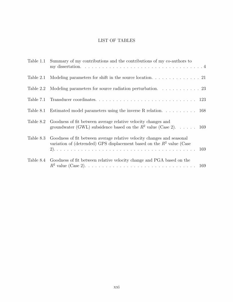
Table 1.1 Summary of my contributions and the contributions of my co-authors tomy dissertation. . . . . . . . . . . . . . . . . . . . . . . . . . . . . . . . . . . 4

Table 2.1 Modeling parameters for shift in the source location. . . . . . . . . . . . . . 21

Table 2.2 Modeling parameters for source radiation perturbation. . . . . . . . . . . . 23

Table 7.1 Transducer coordinates. . . . . . . . . . . . . . . . . . . . . . . . . . . . . 123

Table 8.1 Estimated model parameters using the inverse R relation. . . . . . . . . . 168

Table 8.2 Goodness of fit between average relative velocity changes andgroundwater (GWL) subsidence based on the R2 value (Case 2). . . . . . 169

Table 8.3 Goodness of fit between average relative velocity changes and seasonalvariation of (detrended) GPS displacement based on the R2 value (Case2). . . . . . . . . . . . . . . . . . . . . . . . . . . . . . . . . . . . . . . . . 169

Table 8.4 Goodness of fit between relative velocity change and PGA based on theR2 value (Case 2). . . . . . . . . . . . . . . . . . . . . . . . . . . . . . . . 169

xxi

ACKNOWLEDGMENTS

If I have seen further it is by standing on ye sholders of Giants. The accomplishment of

this dissertation echoes these words from Isaac Newton. The progress in earning my graduate

degree and in the completion of this thesis work has been the result of a huge amount of

support I have received along the way. I doubt the space here is enough to show my true

appreciation and thanks to all who have supported, encouraged, and inspired me.

First, I am grateful to my advisor Dr. Roel Snieder. I first met him briefly during the

CWP meeting at the 2009 SEG Annual meeting in Houston. Then, I came to scout some of

the research groups I was interested in applying to. He was one of those I met on that day

that made me feel comfortable applying to CWP. I later met him again on my first day at

CWP with Yuanzhong Fan (a CWP alumnus), who introduced me to him. I did receive my

first dose of Roel’s jokes during this meeting, some of them I still remember. He’s that kind

of person. He has always been encouraging and funny, even as he demanded the best from

me. I believe I have grown in no small way because of his guidance. This growth includes

the way I now tackle scientific problems and improvement in my communication skills. I

don’t think I am yet where I need to be, but his tutoring gives me the right foundation as I

move forward.

I am grateful to Roel for the opportunity he gave me to work on diverse research projects.

While with him, I have had the opportunities to work with both real and numerical data,

work on both individual and collaborative projects, and acquire research experience in a

couple of oil companies through internships. A lot of these opportunities have come from

his ability to both guide me in the right direction through his suggestions and to give me

the freedom to pursue projects that I have interest in. His guidance and relationship I will

still highly regard even beyond my PhD studies. I am also grateful to the wonderful research

minds of Dan O’Connell, Kristine Pankow, Ernst Niederleithinger, and Andrew Munoz,

xxii

whom I had the opportunity to work with. Our discussions have enormously enriched me

personally and in my thesis work.

I thank the members of my thesis committee - Dr. Masami Nakagawa, Dr. Paul Sava,

Dr. Thomas Davis, Dr. David Wald and Dr. Michael Walls - for all their guidance and

revision of my thesis work. A lot of the advice I have received both during my defenses and

our one-on-one meetings have been useful to improve the quality of this dissertation. I am

also grateful for their encouragement during the di�cult time of the thesis process. I ever

remain grateful. My regard also goes to the faculty and students of CWP and the Geophysics

Department in general. I am grateful for colleagues and friends who in no small ways have

made the last four years wonderful. The diversity both in research interests and personal

backgrounds was what drew my interest to this research group. I wasn’t disappointed but

rather gained far more than I could imagine. CWP’s demand on its students to develop into

well-rounded scientists in terms of the content of their research, the communication of their

work, and direct interaction with the big players in industry is unmatched. Fan, my o�cial

graduate buddy the year I joined CWP, deserves credit. He was my first contact with CWP

during our SEG/Exxonmobil SEP program. I later learned that his recommendation was

instrumental to my joining CWP as a graduate student. Fan, thank you.

Diane Witters, I am really grateful for your help with all the writing, communication, and

pronunciation skills. My meetings with Diane opened my eyes to the nuances of technical

writing, made me aware of the common mistakes I make, and helped me work on the clarity

of my oral delivery. Although I am far from where she will want me to be at mastering these

skills, I now have the confidence to critically evaluate my own writing and communication.

I am at times amazed at her patience. Thank you, Diane, for your help and encouragement

which have, in a lot of ways, made this dissertation a reality. I am also grateful to Pamela

Kraus, Shingo Ishida, John Stockwell and Michelle Szobody for their help with administrative

details surrounding my PhD studies which have allowed me to concentrate on my research.

xxiii

My journey through graduate school started when Dr. G. U. Chukwu, one of my under-

graduate lecturers, pointed my attention to the scholarship program in Earth System Physics

at International Center for Theoretical Physics (ICTP), Italy. This opportunity opened the

door to the rest of my graduate studies. I am immensely grateful to him for his foresight.

I am really grateful to my parents and sisters back in Nigeria. Their patience with me

throughout all the process of graduate school since I left home about seven years ago cannot

be matched. I am sincerely grateful for their prayers, belief, support, jokes, and stories. I

do own them all.

xxiv

To Almighty God

xxv

CHAPTER 1

INTRODUCTION

Time-lapse monitoring tools in geophysics provide ways for monitoring changes within the

earth, geomechanical structures, and mechanical structures. The information inferred from

the observed changes can be used to describe various geomechanical or mechanical processes,

such as fluid migration and geological or structural deformations, within the medium in

which the change occurs. Time-lapse monitoring is used in petroleum engineering activities

such as in hydrocarbon production and fluid injection [22, 43], in global seismology such as

for monitoring volcanic activities [56, 88] and for preseismic to post-seismic deformations

near and far away from fault rupture zones [16, 117], in geohazard evaluations such as for

monitoring stress changes in the near surface [62, 89] and in monitoring mechanical structures

like cracks or defects in buildings, roads, and machines [31, 100]. Various monitoring methods

and tools are used for characterizing time-lapse changes. These monitoring tools di↵er from

one disciplinary field to another depending on what the monitoring objectives are.

The challenge of monitoring with seismic waves depends, in general, on whether the waves

are transmitted, singly scattered, or multiply scattered within the scattering medium. Usu-

ally the complexity of the waves with respect to the scattering medium increases from trans-

mitted waves (direct or diving waves) to the multiply scattering waves. However, increased

scattering of the waves within the scattering medium usually provides better illumination

of the scattering medium [26, 28], additional redundancy that is useful for improving the

resolution and increasing the signal-to-noise ratio of images [8, 9], and increased sensitivity

of the waves to changes within the scattering medium [97, 108]. Coda wave interferome-

try provides a means of monitoring weak changes with multiply scattered waves, especially

changes which are poorly detected by singly scattered waves [76]. The challenge in using

1

multiply scattered waves for monitoring weak and localized time-lapse changes, in order to

take advantage of their increased sensitivity, is to develop a relatively cheap and e�cient

way of imaging the time-lapse changes with multiply scattered waves.

In this dissertation, I work with both numerical and field-collected multiply scattered

waves (coda waves), which I use to study the capability of monitoring and imaging weak

localized time-lapse changes within scattering media. The scattering media to which we

apply this work cover a wide range of structures from the geological subsurface to mechanical

structures. Specifically, we use scattered waves generated within the earth’s subsurface

for time-lapse monitoring of the eastern part of the Basin and Range in the western US

(Chapter 8) and ultrasonic waves generated within heterogeneous concrete blocks for time-

lapse monitoring of localized changes within the blocks due to either stress or temperature

changes (Chapters 6 and 7). We also perform a number of numerical tests to characterize

other scattering media.

In Chapter 2, I explore the use of time-lapse scattered waves generated by repeating

sources with varying source properties; specifically, I analyze the impact of di↵erences in their

locations and focal mechanisms. The focus in this chapter is to characterize the limits of the

repeating sources generating the time-lapse scattered waves; the repeating sources we can

use for monitoring time-lapse velocity changes within a scattering medium. Understanding

these limits allows us to pick sources for the time-lapse scattered waves within a pre-defined

region and a range of source radiation angles, without working under the strong restriction

of using perfectly repeating scattering signals. This is vital in cases where we have limited

control over the sources such as when using the coda from earthquakes or microseismic events

for time-lapse monitoring. I use simple numerical models with a homogeneous distribution

of scatterers and a uniform time-lapse velocity change in the scattering models. I define

a limiting criterion for selecting the maximum allowable distance between the repeating

sources, and suggest the use of the maximum cross-correlation of the time-lapse coda as a

proxy for the error due to the deviation in the source radiation angles.

2

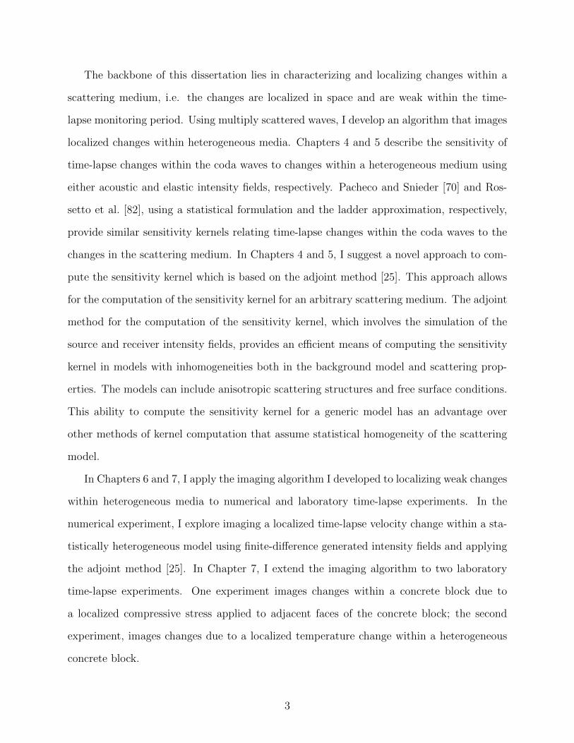
The backbone of this dissertation lies in characterizing and localizing changes within a

scattering medium, i.e. the changes are localized in space and are weak within the time-

lapse monitoring period. Using multiply scattered waves, I develop an algorithm that images

localized changes within heterogeneous media. Chapters 4 and 5 describe the sensitivity of

time-lapse changes within the coda waves to changes within a heterogeneous medium using

either acoustic and elastic intensity fields, respectively. Pacheco and Snieder [70] and Ros-

setto et al. [82], using a statistical formulation and the ladder approximation, respectively,

provide similar sensitivity kernels relating time-lapse changes within the coda waves to the

changes in the scattering medium. In Chapters 4 and 5, I suggest a novel approach to com-

pute the sensitivity kernel which is based on the adjoint method [25]. This approach allows

for the computation of the sensitivity kernel for an arbitrary scattering medium. The adjoint

method for the computation of the sensitivity kernel, which involves the simulation of the

source and receiver intensity fields, provides an e�cient means of computing the sensitivity

kernel in models with inhomogeneities both in the background model and scattering prop-

erties. The models can include anisotropic scattering structures and free surface conditions.

This ability to compute the sensitivity kernel for a generic model has an advantage over

other methods of kernel computation that assume statistical homogeneity of the scattering

model.

In Chapters 6 and 7, I apply the imaging algorithm I developed to localizing weak changes

within heterogeneous media to numerical and laboratory time-lapse experiments. In the

numerical experiment, I explore imaging a localized time-lapse velocity change within a sta-

tistically heterogeneous model using finite-di↵erence generated intensity fields and applying

the adjoint method [25]. In Chapter 7, I extend the imaging algorithm to two laboratory

time-lapse experiments. One experiment images changes within a concrete block due to

a localized compressive stress applied to adjacent faces of the concrete block; the second

experiment, images changes due to a localized temperature change within a heterogeneous

concrete block.

3

A vital part of the work in this dissertation involves the extraction of the time-lapse

changes (travel-time shifts) within the multiply scattered waves. In Chapter 3, I explore the

used of dynamic time warping (DTW) algorithm [35] for time shift extractions in order to

characterize their strengths and weaknesses in regard to time-lapse monitoring of the weak

changes within scattering media. I compared the DTW algorithm with two existing methods

(time-shift cross-correlation and stretching methods) for estimating travel-time change within

time-lapse coda waves. In Chapter 8, I apply coda wave interferometry to monitor time-lapse

velocity changes within the subsurface beneath the eastern flank of the Basin and Range.

This region is an actively deforming region of the western US and the study suggests a

consistent velocity change of less than 0.2 % within a time period of 5 months. Comparison

of the velocity changes with temporal variation of the E-W strain suggests that the velocity

change is driven by the extensional deformation within Basin and Range.

Table 1.1: Summary of my contributions and the contributions of my co-authors to mydissertation.

Chapter My contribution Contribution of others2 Define sensitivity analysis and con-

ducted numerical analysisDiscussion on monitoring with micro-seismicity with Dan O’Connell

3 Develop cross-correlation/stretchingcodes

Andrew Munoz developed (S)-DTWcodes

7 Develop inversion code and doing inver-sions

Setup of laboratory experiment andtime-lapse data collection by S.Grotheand E. Niederleithingher (BAM).

8 Data analysis, code development andanalytical/numerical analysis

Collection of time-lapse data via IRISand GPS measurements by K. Pankow.

4/5/6 Develop novel computation of sensitiv-ity kernel, code development, and nu-merical analysis

My contribution to the field of geophysics and time-lapse monitoring via this dissertation,

is the development and implementation of an approach to image localized and weak changes

present within statistically heterogeneous media using multiply scattered waves. The changes

my imaging algorithm provides spatial resolution to include velocity changes within volca-

4

noes, geomechanical perturbations within stimulated or depleting hydrocarbon reservoirs,

changes in the thermal properties of an enhanced geothermal system (EGS), defects within

mechanical structures and tumors within the human body. I developed the theoretical and

the numerical background of all the studies presented in this dissertation. Table 1.1 gives a

brief description of the contributions of my co-authors. I used the Madagascar open-source

software package (http://www.ahay.org) to develop the numerical codes I used to compute

the sensitivity kernels. Other codes I used for data analysis, various numerical tests and

inversion, I developed using the MATLAB software.

The work in this dissertation is, or will be, documented in the following publications:

Chapter 2: Kanu, C.O., R. Snieder, and D. O’Connell (2013), Estimation of veloc-

ity change using repeating earthquakes with di↵erent locations and focal mechanisms, J.

Geophys. Res. Solid Earth, 118, 29052914, doi:10.1002/jgrb.50206.

Chapter 4: Kanu, C.O., and R. Snieder, Numerical computation of the sensitivity

kernel for time-lapse monitoring with multiply scattered acoustic waves, Geophysical Journal

International. (submitted).

Chapter 5: Kanu, C. O., and R. Snieder, Numerical computation of the sensitivity

kernel for time-lapse monitoring with multiply scattered elastic waves, Geophysical Journal

International. (submitted).

Chapter 6: Kanu, C. O., and R. Snieder, Time-lapse imaging of localized weak changes

with multiply scattered waves: Numerical experiment, Journal Geophysical Research (sub-

mitted).

Chapter 7: Kanu, C. O., R. Snieder, E. Niederleithingher, and S. Grothe, Time-lapse

imaging of localized weak changes with multiply scattered waves: Laboratory experiment,

Ultrasonics (submitted).

Chapter 8: Kanu, C., R. Snieder, and K. Pankow (2014), Time-lapse monitoring of

velocity changes in Utah, J. Geophys. Res. Solid Earth, 119, doi:10.1002/2014JB011092.

5

CHAPTER 2

ESTIMATION OF VELOCITY CHANGE USING REPEATING EARTHQUAKES WITH

DIFFERENT LOCATIONS AND FOCAL MECHANISMS

Chinaemerem O. Kanu1, Roel Snieder1 and Dan O’Connell2

Published in Journal Geophysical Research (2013)

2.1 Abstract

Codas of repeating earthquakes carry information about the time-lapse changes in the

subsurface or reservoirs. Some of the changes within a reservoir change the seismic velocity

and thereby the seismic signals that travel through the reservoir. We investigate, both

theoretically and numerically, the impact of the perturbations in seismic source properties

of used repeating earthquakes on time-lapse velocity estimation. We derive a criterion for

selecting seismic events that can be used in velocity analysis. This criterion depends on

the dominant frequency of the signals, the centertime of the used time window in a signal,

and the estimated relative velocity change. The criterion provides a consistent framework

for monitoring changes in subsurface velocities using microseismic events and the ability to

assess the accuracy of the velocity estimations.

2.2 Introduction

Monitoring temporal changes within the Earth’s subsurface is a topic of interest in many

areas of geophysics. These changes can result from an earthquake and its associated change

in stress [16], fluid injection or hydrofracturing [22], and oil and gas production [116]. Some

of the subsurface perturbations induced by these processes include temporal and spatial ve-

locity changes, stress perturbations, changes in anisotropic properties of the subsurface, and

1Center for wave phenomena, Colorado School of Mines2Fugro Consultants, Inc., William Lettis Associates Division, Lakewood, CO 80401

6

fluid migration. Many of these changes span over a broad period of time and might even

influence tectonic processes, such as induced seismicity [117]. For example, Kilauea, Hawaii

(which erupted in November 1975) is suggested to have triggered a magnitude 7.2 earthquake

within a half hour of the eruption [47]. A seismic velocity perturbation of the subsurface

leads to progressive time shifts across the recorded seismic signals. Various methods and data

have been used to resolve the velocity perturbations. These methods include seismic coda

wave interferometry [97], doublet analysis of repeating microseismic and earthquake codas

[76], time-lapse tomography [107], and ambient seismic noise analysis [12, 16, 58, 88, 111].

Earthquake codas have higher sensitivity to the changes in the subsurface because multi-

ple scattering allows these signals to sample the area of interest multiple times. However,

there are inherent challenges in the use of these signals. Doublet analysis of the earthquake

(microseismic) codas requires repeating events. Failure to satisfy the requirement that the

events are identical can compromise the accuracy of the estimated velocity changes. In this

study, we focus on the estimation of velocity changes using codas of repeating earthquakes

that are not quite identical in their locations and source mechanisms.

Fluid-triggered microseismic events often are repeatable, but in practice events occur at

slightly di↵erent positions with somewhat di↵erent source mechanisms [30, 59, 85]. Changes

in the source properties might result from coseismic stress changes [5] or changes in the

properties of the event rupture locations [57]. Imprints of the source perturbation and the

velocity change on the seismic waveforms can be subtle. Therefore, we will need to ask, how

do the source location, source mechanism, and subsurface perturbations a↵ect the estimated

velocity changes? Snieder [96] shows that we can retrieve velocity changes from the coda

of the waveforms recorded prior to and after the change. Robinson et al. [79] develop a

formulation using coda wave interferometry to estimate changes in source parameters of

double-couple sources from correlation of the coda waves of doublets. Snieder and Vrijlandt

[99], using a similar formulation, relate the shift in the source location to the variance of

the travel time perturbations between the doublet signals. In all these studies, the authors

7

assume that the expected (average) change in travel time of the coda (due to either changes

in the source locations or source mechanisms) is zero.

In this study, we investigate the impact of changes in source properties on the estimation

of relative velocity changes. Knowledge of the impact of these perturbations on the esti-

mated velocity change allows for a consistent framework for selecting pairs of earthquakes or

microearthquakes used for analyzing the velocity changes. This results in a more robust es-

timation of velocity change. In Section 2.3, we explore the theoretical relationships between

the velocity changes and perturbations in the earthquake source properties. Following this

section is a numerical validation of the theoretical results. We explain the implications and

limitations of our results in Section 2.5. In the appendices, we explain the mathematical

foundation of our results in this study.

2.3 Mathematical Consideration

In this section, we use the time-shifted cross-correlation [96, 97] to develop an expression

for the average value of the time perturbation of scattered waves that are excited by sources

with varying source properties. This perturbation is due to changes in the velocity of the

subsurface and to changes in the source properties. These changes, we assume, may occur

concurrently. Figure 2.1 is a schematic figure showing the general setup of the problem we are

investigating. Two sources (S1 and S2) represent a doublet (repeating seismic events). These

events occur at di↵erent locations and may have di↵erent rupture patterns. We assume that

these events can be described by a double couple. We investigate the ability of using the

signals of these sources for time-lapse monitoring of velocity changes, assuming that these

sources occur at di↵erent times. We express the signals of the two sources as unperturbed

and perturbed signals, where the perturbation refers to any change in the signal due to

changes within the subsurface and/or the source properties.

The unperturbed seismic signal U(t) is given as

U(t) = AX

T

U (T )(t) (2.1)

8

Receiver

Scatterers

Path T

Path T’

S2

S1

D

LT LT’

rT

Figure 2.1: Geometry of wave paths. Source, S1, produces the unperturbed signal whileSource, S2, produces the perturbed signal. Path T shows the scattering path for the unper-turbed signal and the scattering path for the perturbed signal is defined by Path T 0. Thesources are separated by a distance D and the source distances are L

T

and LT

0 distance awayfrom the first scatterer along path T and T 0, respectively. The unit vector r

T

defines thedirection traveled by the signal before the signal first encounters a scatterer.

9

and the perturbed seismic signal U(t) is given as

U(t) = AX

T

(1 + ⇣(T ))U (T )(t� tTp

), (2.2)

where A and A are the amplitudes of the unperturbed and perturbed source signals, respec-

tively. These amplitudes represent the strengths of the sources. The recorded waves are a

superposition of wave propagation along all travel paths as denoted by the summation over

paths T . The change in the source focal mechanism only a↵ects the amplitude of the wave

traveling along each trajectory T because the excitation of waves by a double couple is real

[2]. The change in the signal amplitudes - due to changes in the source mechanism angles -

is defined by ⇣(T ) for path T , and tTp

is the time shift on the unperturbed signal due to the

medium perturbation for path T . The change in the signal amplitudes along path T depends

on the source radiation angles. In this study, we assume that the medium perturbation re-

sults from the velocity change within the subsurface and changes in the source properties.

The time-shifted cross-correlation of the two signals is given as

C(ts

) =

Zt+t

w

t�t

w

U(t0)U(t0 + ts

) dt0, (2.3)

where t is the centertime of the employed time window and 2tw

is the window length. The

normalized time-shifted cross-correlation R(ts

) can be expressed as follows:

R(ts

) =

Rt+t

w

t�t

w

U(t0)U(t0 + ts

) dt0

(R

t+t

w

t�t

w

U2(t0) dt0R

t+t

w

t�t

w

U2(t0) dt0)12

. (2.4)

The time-shifted cross-correlation has a maximum at a time lag equal to the average time

perturbation (ts

= htp

i) of all waves that arrive in the used time window [96]:

@C(ts

)

@ts

��(t

s

=htp

i)= 0. (2.5)

Equation 2.5 allows for the extraction of the average travel-time perturbation from the cross-

correlation. In this study, the average of a quantity f is a normalized intensity weighted sum

of the quantity [96]:

hfi =P

T

A2T

fTP

T

A2T

, (2.6)

10

where A2T

=R(UT (t0))2 dt0 is the intensity of the wave that has propagated along path T .

We show in Appendices A and B that the expected value of the time perturbation and

its variance are given by

htp

i = �D�VVo

Et (2.7)

and

�2t

= ht2p

i � htp

i2 ' D2

3V 20

. (2.8)

In the above equations, h�V/V0i is the average relative velocity change, D is the shift in the

source location, and V0 is the unperturbed velocity of a wave mode. This result is applicable

to any wave mode. Equation 2.7 suggests that the average time shift in the multiple scattered

signals depends only on the velocity changes within the subsurface. The variance of the time

shifts depends, however, on the perturbations of the source location.

2.4 Numerical Validation

We test the equations in section 2.3 with a numerical simulation using Foldy’s multiply

scattering theory [27] described by Groenenboom [32]. The theory models multiple scattering

of waves by isotropic point scatterers. We conduct our numerical experiments using a circular

2D geometry (Figure 2.2) with point scatterers surrounded by 96 receiver stations. We

uniformly assign the imaginary component of the scattering amplitude ImA = -4 to all the

scatterers. In 2D, this is the maximum scattering strength that is consistent with the optical

theorem that accounts for conservation of energy [32]. The wave radiated by the earthquakes

is modulated by the far-field P-wave radiation pattern F P :

U0(r) = F PG(0)(r, rs

), (2.9)

where G(0)(r, rs

) is the green’s function between the source location rs

and any other point

r. In 2D, where the take-o↵ direction is restricted within the 2D plane, F P is given as [2]

F P = cos� sin � sin 2( � �)� sin� sin 2� sin2 ( � �), (2.10)

11

−15 −10 −5 0 5 10 15−15

−10

−5

0

5

10

15

West−East (km)

So

uth

−N

ort

h (

km)

E

SW

NW NE

SE

W

Figure 2.2: The experiment geometry of the numerical simulation. The receivers (squares)are surrounding the point scatterers (black dots). The source is positioned in the origin(cross). All perturbations of the source location is done from this position. The stationsmarked (NW, NE, E, SE, and SW) are used in the presentation of results in Figure 2.7 andFigure 2.8.

12

where is the azimuth of the outgoing wave and �, �, and � are the source parameters (rake,

dip and strike, respectively). Sources are located at the center of the scattering area. The

source spectrum has a dominant frequency fd

of approximately 30 Hz and a frequency range

of 10-50 Hz. The source spectrum tapers o↵ at the frequency extremes by a cosine taper

with a length given by half of the bandwidth. We assume a reference velocity V0 = 3500

m/s. Because the model we are using is an isotropic multiple scattering model, the transport

mean free path is the same as the scattering mean free path: l⇤ = l. The scattering mean

free path l⇤ [14, 32] is given by

l⇤ =ko

⇢|ImA| , (2.11)

where ko

is the wavenumber of the scattered signal and ⇢ is the scatterer density. For our

model, the mean free path l⇤ is approximately 30.5 km. There is no intrinsic attenuation in

the numerical model.

We generate multiple scattered signals, which are recorded at the receivers, using the

numerical model in Figure 2.2. These signals are generated with a reference model defined

by the following reference parameter values: the source radiation parameters � = 0o, � =

0o, � = 90o; change in medium velocity �V = 0 m/s; and shift in the source location D = 0

m. We refer to signals generated by this reference model as the reference signals. In order to

understand the e↵ect of the perturbation of these parameters on velocity change estimation,

we also generate synthetic signals from the perturbed version of the model. The perturbed

model consists of perturbation of either the source locations, source radiation parameters, the

medium velocity, or a combination of these. Synthetic signals from the reference and the 0.4%

velocity perturbed models are shown in Figure 2.3I with zoom insets showing the stretching

of the waveform by the velocity perturbation. The result of the velocity perturbation on

the signals is a progressive time shift of the arriving seismic phases in the signals. Similarly,

the e↵ect of the independent perturbation of the source locations and the source radiation

parameters are shown in Figure 2.3II and Figure 2.3III, respectively. The source location

perturbation is 0.14�d

along the z direction and the source radiation perturbation is 20o for

13

0 5 10 15 20 25 30−1

−0.5

0

0.5

1

Time (s)

No

rma

lize

d A

mp

litu

de A

B

3.2 3.3 3.4 3.5 3.6 3.7−1

−0.5

0

0.5

1

Time (s)

No

rma

lize

d A

mp

litu

de

13 13.1 13.2 13.3 13.4 13.5 13.6−0.2

−0.1

0

0.1

0.2

Time (s)

No

rma

lize

d A

mp

litu

de

0 5 10 15 20 25 30−1

−0.5

0

0.5

1

Time (s)

No

rma

lize

d A

mp

litu

de

13 13.1 13.2 13.3 13.4 13.5 13.6−0.2

−0.1

0

0.1

0.2

Time (s)

No

rma

lize

d A

mp

litu

de

3.2 3.3 3.4 3.5 3.6 3.7−1

−0.5

0

0.5

1

Time (s)

Norm

aliz

ed A

mplit

ude

A

B

0 5 10 15 20 25 30−1

−0.5

0

0.5

1

Time (s)

No

rma

lize

d A

mp

litu

de A

B

13 13.1 13.2 13.3 13.4 13.5 13.6−0.2

−0.1

0

0.1

0.2

Time (s)

No

rma

lize

d A

mp

litu

de

3.2 3.3 3.4 3.5 3.6 3.7−1

−0.5

0

0.5

1

Time (s)

No

rma

lize

d A

mp

litu

de

I

II

III

Figure 2.3: Recorded seismic signals at station E (Figure 2.2), the reference signal (red line)and the time-lapse signal (black line) with 0.4% relative velocity change (I), the time-lapsesignal (black line) with 0.14�

d

source displacement (II), and the time-lapse signal (black line)with 20o source angle perturbations (III). Inset A shows the late coda while inset B showsthe first arrivals of the two signals. The black bold line is the time window used for dataprocessing. Time 0 is the source rupture time.

14

both the strike, rake and dip angles. The zoom insets in these Figure 2.3II and Figure 2.3III

show that the changes in the source properties result in amplitude di↵erences between the

time-lapse signals. There are also phase di↵erences between the time-lapse signals due to

the perturbation of the source locations.

2.4.1 Data processing

To estimate the velocity perturbations or possible velocity change imprints on the syn-

thetic signals due to the perturbation of the source location or its radiation properties, we

use the stretching algorithm of Hadziioannou et al. [33] who demonstrate the stability and

robustness of the algorithm relative to the moving time-window cross-correlation of Snieder

et al. [97] and the moving time-window cross-spectral analysis of Poupinet et al. [76]. Both

algorithms satisfy the relative velocity change equation [96]:

*tp

t

+= �✏, (2.12)

where ✏ = h�V/Vo

i is the relative velocity change.

In the stretching algorithm, we multiply the time of the perturbed signal with a stretching

factor (1� ✏) and interpolate the perturbed signal at this stretched time. The time window

we use in all our analysis is given by the black bold line in Figure 2.3. We then stretch the

perturbed signal at a regular interval of ✏ values. The range of the ✏ values can be arbitrarily

defined or predicted by prior information on the range of changes in the subsurface velocity.

To resolve the value of ✏, we use an L2 objective function rather than the cross-correlation

algorithm as suggested by Hadziioannou et al. [33]. For events of equal magnitude (A = A),

the objective function is

R(✏) = ||U(t(1� ✏))� U(t)||2, (2.13)

where ||...||2 is the L2 norm. Figure 2.4 shows the objective function based on the L2 norm

and the maximum cross-correlation for the case of a 0.4% velocity change. The L2 norm

more accurately constrains the velocity change than the maximum cross-correlation. The

15

minimum of the objective function based on the L2 norm depends on the amplitude changes

between the two signals and on the travel time perturbations due to velocity changes and

shifts in the source location. The signals have uniform magnitudes. The amplitude changes

between the signals are due to changes in the orientation of the source angles.

The error in the estimated relative velocity change ��v

is given by

��v

�U

2⇡fd

At, (2.14)

where fd

is the dominant frequency, t is the centertime of the signal, A is the amplitude of

the signals, and �U

is the standard deviation of the recorded waveforms. The derivation of

equation 2.14 is given in Appendix C. The error associated with the velocity change depends

on additive noise in the signals and on di↵erences in the signals both in amplitude and in

phase due to perturbation in source properties.

2.4.2 E↵ect of perturbation of source properties on the estimated velocitychange

To understand the e↵ect of the changes in the source properties on the estimation of the

relative velocity changes, we conduct our numerical experiment over a range of parameter

changes. We perturb the source location and the orientation of the source angles. The

perturbation of the source radiation parameters is characterized by the weighted root mean

square change in source parameters h⇣i [80]:

h⇣i = �1

2(4��2 +��2 +��2), (2.15)

where �� is the change in strike, �� is the change in rake, and �� is the change in dip,

between the two sources.

Figure 2.5 and Figure 2.6 show the estimated velocity changes due to the perturbation of

medium velocity and the source properties (location and radiation parameters), respectively.

For Figure 2.5, we generate signals with the following perturbation in the model velocity

h�V/V0i: 0.1%, 0.2%, 0.3%, and 0.4%. In these models, we keep the source parameters un-

changed. Using the stretching method, we are able to recover the velocity changes we impose

16

−0.02 −0.01 0 0.01 0.020

0.1

0.2

0.3

0.4

0.5

0.6

0.7

0.8

0.9

1

Stretch factor (relative velocity change)

Ob

ject

ive

fu

nct

ion

Max. CorrelationLeast−squares norm

Figure 2.4: The objective function R(✏) (solid line) as a function of the stretch factor ✏. Theobjective function is minimum for ✏ = 0.4%, which corresponds to the time-lapse velocitychange. The corresponding maximum correlation of the stretch factors is given by the dashlines.

17

0 20 40 60 80 1000

0.1

0.2

0.3

0.4

0.5

0.6

Receiver number

Re

lativ

e v

elo

city

ch

an

ge

(%

)

0.1%0.2%0.3%

0.4%

Figure 2.5: Estimated relative velocity change for model velocity change of h �VV0i = 0.1%

(blue), h �VV0i = 0.2% (red), h �V

V0i = 0.3% (black), and h �V

V0i = 0.4% (green). The receiver

numbers are counted counter-clockwise from the W station in Figure 2.2.

18

0 20 40 60 80 100−0.02

−0.01

0

0.01

0.02

D/λ = 0.036D/λ = 0.07D/λ = 0.107D/λ = 0.143

Re

lativ

e V

elo

city

Ch

an

ge

(%

)

1d

d

d

d

0 20 40 60 80 100−0.02

−0.01

0

0.01

0.02

Receiver Number

ζ = −0.022ζ = −0.091ζ = −0.206ζ = −0.366

A

B

Figure 2.6: Estimated relative velocity change due to perturbation in the source locationand the source radiation. A. The estimated velocity change for perturbed source location(divided by the dominant wavelength; inset in the top right) and B. The estimated velocitychange caused by changes in source radiation angles (inset in the top right). The value of ⇣is given by equation 2.15. The receiver numbers are counted counter-clockwise from the Wstation in Figure 2.2.

19

in the model from the codas of each of the perturbed signals and that of the reference signal

(Figure 2.5). The method accurately estimates the model velocity change in all the receivers.

We also generate signals with perturbations in the source locations and mechanisms only.

In this case, the true velocity change is zero. Figure 2.6 shows that the estimated relative

velocity changes h�V/Vo

i are near the true value (�V = 0) for models with perturbations of

either the source location or the source radiation parameters. The velocity change estimated

from individual stations varies around zero, but with a shift in the source location of D =

0.143�d

, with �d

the dominant wavelength and source angle perturbations as large as ��

= 20o, �� = 20o, and �� = 20o (h⇣i = -0.366), the magnitude of the estimated velocity

change is smaller than 1/20th of the typical velocity changes inferred from seismic signals

(Figure 2.6). These variations in the velocity change inferred from di↵erent stations can

be used to estimate the errors in the estimated velocity change. These results agree with

equation 2.7 which predicts that the average value of time shifts in the perturbed signal

results only from changes in the medium velocity and is not a↵ected by changes in source

properties. We will need to know how e↵ectively we can resolve the velocity changes in our

model in the presence of the other model parameter perturbations.

2.4.3 Limiting regimes of the estimations

To investigate the extent of the perturbation in the source location and source radiation

perturbations that can be allowed in the estimation of relative velocity changes, we generate

synthetic signals with models having a 0.1% relative velocity change and various perturba-

tions of the source parameters. The values of the source parameter perturbations are given

in Table 2.1 and Table 2.2. Figure 2.7 shows the estimated relative velocity changes from

signals generated from sources at di↵erent locations. The figure shows that we can recover

the relative velocity change of 0.1% using doublets (two sources) within a sphere of radius

�d

/4 , where �d

is the dominant wavelength of the seismic signal which is approximately 140

m. This is consistent with the criterion we derived in Appendix D, which predicts that for

an accurate estimation of the subsurface velocity change, the shift in the source location has

20

to satisfy

D

�d

<p2

��

*�V

Vo

+��fdt, (2.16)

where fd

is the dominant frequency of the signals, h�V/V0i is the average velocity change in

the subsurface, and t is the centertime of the processed signal. The criterion is derived from

a comparison of the phase changes due to velocity changes with those due to shifts in the

source location. For the results in Figure 2.7, our model parameters are h�V/Vo

i = 0.1%, t

= 10 s, and fd

' 25 Hz. With these values, the constraint on the source location shift for

Figure 2.7 is

D

�d

< 0.35. (2.17)

Table 2.1: Modeling parameters for shift in the source location.

Case �V

V

(%) D/�d

Reference 0 0Case 1 0.1 0.0274Case 2 0.1 0.0547Case 3 0.1 0.0820Case 4 0.1 0.1094Case 5 0.1 0.1367Case 6 0.1 0.1642Case 7 0.1 0.1918Case 8 0.1 0.2197Case 9 0.1 0.2477Case 10 0.1 0.2760Case 11 0.1 0.3047Case 12 0.1 0.3337Case 13 0.1 0.3627Case 14 0.1 0.3916Case 15 0.1 0.4202

Figure 2.7 shows that for D/�d

� 0.3, the estimated velocity change deviates significantly

from the real velocity change; this is in agreement with equation 2.17. The criterion in equa-

tion 2.16 imposes a constraint on the spacing requirements for the source locations of the

doublets used for time-lapse velocity change monitoring with microearthquakes. Alterna-

21

0 0.1 0.2 0.3 0.4 0.5−0.6

−0.4

−0.2

0

0.2

0.4

0.6

Source location shifts (D/λ )

Re

lativ

e v

elo

city

ch

an

ge

(%

)

Station SWStation SEStation NEStation NW

d

D

λd

< 0.35

Figure 2.7: Estimated relative velocity change after a 0.1% velocity change and varioussource location perturbations (Table 2.1). The shift in the source locations are divided bythe dominant wavelength �

d

of the recorded signals. For values of the source location shiftgreater than �

d

/4, we have incorrect estimates for the velocity change due to the distortionof the perturbed signal. Stations SW, SE, NE, and NW positions are given in Figure 2.2.The red line indicates the model (accurate) velocity change.

22

Table 2.2: Modeling parameters for source radiation perturbation.

Case �V

V

��(o) ��(o) ��(o) �h⇣iReference 0 0 0 0 0Case 1 0.1 0 0 0 0Case 2 0.1 2 2 2 0.0037Case 3 0.1 4 4 4 0.0146Case 4 0.1 6 6 6 0.0329Case 5 0.1 8 8 8 0.0585Case 6 0.1 10 10 10 0.0914Case 7 0.1 12 12 12 0.1316Case 8 0.1 14 14 14 0.1791Case 9 0.1 16 16 16 0.2339Case 10 0.1 18 18 18 0.2961Case 11 0.1 20 20 20 0.3655Case 12 0.1 22 22 22 0.4423Case 13 0.1 24 24 24 0.5264Case 14 0.1 26 26 26 0.6178Case 15 0.1 28 28 28 0.7165

tively, equation 2.16 gives the magnitude of a velocity change that is resolvable with a given

shift in the source location. According to equation 2.16, the allowable source separation

increases with the centertime t of the employed time window. This is due to the fact that

the imprint of the velocity change is more pronounced as the waves have propagated over a

greater distance through the perturbed medium. However, signals at later times in the coda

are more a↵ected by the presence of additive noise because the signal-to-noise ratio usually

decreases towards the late coda.

We also investigate the e↵ect of the source radiation properties on the estimated velocity

change of the medium of interest. Figure 2.8 shows the estimated velocity changes from a

model with 0.1% velocity change using sources with perturbed radiation angles (measured

by h⇣i). The values of the perturbed source radiation angles are given in Table 2.2. In Fig-

ure 2.8A, the estimated velocity change at the individual stations progressively deviates from

the true velocity change of 0.1% with increasing change in the orientations of the source an-

gles. This deviation is due to the decorrelation between the perturbed and the unperturbed

23

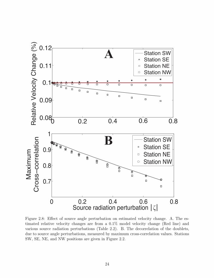
0 0.2 0.4 0.6 0.8

0.7

0.8

0.9

1

Source radiation perturbation ζ

Ma

xim

um

Cro

ss−

co

rre

latio

n


0 0.2 0.4 0.6 0.80.08

0.09

0.1

0.11

0.12

Re

lativ

e V

elo

city

Ch

an

ge

(%

)


A

B

Figure 2.8: E↵ect of source angle perturbation on estimated velocity change. A. The es-timated relative velocity changes are from a 0.1% model velocity change (Red line) andvarious source radiation perturbations (Table 2.2). B. The decorrelation of the doublets,due to source angle perturbations, measured by maximum cross-correlation values. StationsSW, SE, NE, and NW positions are given in Figure 2.2.

24

signals as shown in Figure 2.8B, which shows the maximum normalized cross-correlation of

the codas within the processed time window. With an increasing change in the orientation

of the sources, the maximum cross-correlation value of the waves excited by the doublets

decreases. However, for source angle perturbations as large as �� = 28o, �� = 28o, and ��

= 28o, which corresponds to |h⇣i| = 0.72 (Figure 2.8A), the maximum deviation from the

0.1% model velocity change is approximately 0.01%. This is a small change compared to

velocity changes resolved from seismic signals in practice. The maximum cross-correlation

(Figure 2.8B) can be retrieved from the data and can be used as a diagnostic of the ac-

curacy of the estimated velocity change. In this example, a maximum cross-correlation of

0.7 indicates an error of about 10% in the estimated velocity change. The di↵erence in the

errors observed among the 4 stations (SW, SE, NE and NW) is due to the di↵erences in the

amplitude perturbations resulting from the changes in the source angles. Figure 2.9 shows

that with source angle perturbations of �� = 20o, �� = 20o, and �� = 20o the loops in the

radiation pattern in the NE and SW directions change more dramatically than those in the

NW and SE directions. For the parameters used in this experiment, the transport mean free

time t⇤, defined as the time over which the scattered waves loses their directions, is given

by t⇤ = l⇤/c = 8.7 s. c is the propagation velocity of the scattered waves. The time interval

used for the analysis of the coda waves is 3.6 to 20 s (Figure 2.3). This means that the coda

waves in the early part of the time interval used still retains information about the direction

in which they were radiated. The changes in the radiation pattern thereby result to a higher

error in velocity changes estimated with stations NE and SW than those with stations NW

and SE.

2.5 Discussion and Conclusion

In this study, we investigate the influence of perturbation in source properties (location

and radiation) on the estimation of velocity changes. These velocity changes are extracted

from multiply scattered signals (codas) of repeating events. We show that we can resolve

accurate values of relative velocity changes if the shift in the source location satisfies equa-

25

0.5

1

30

210

60

240

90

270

120

300

150

330

180 0

SW

NW

SE

NE

∆φ = ∆λ = ∆δ = 0

∆φ = ∆λ = ∆δ = 20

0

0

Figure 2.9: Source radiation pattern of the modeled earthquake sources before and aftersimultaneous perturbation of the source angles (strike ��, rake �� and dip ��) of 20 degreeeach.

26

tion 2.16. This constraint depends on the dominant frequency of the signal, the estimated

relative velocity change, and the centertime of the employed time window. This places a

restriction on the relative event locations that can be used to estimate the relative velocity

change of the subsurface. However, to use this constraint, we need to know the magnitude of

the relative velocity change we seek to measure. Preliminary results on the velocity change

can be used to pick events satisfying equation 2.16 for an accurate estimation of the velocity

changes. Using doublets that do not satisfy the constraint result in an inaccurate estimate

of the velocity change. Weaver et al. [110] similarly showed that changes in noise sources

induce error in velocity change estimated from correlation signals obtained from the noise

signals. Although our study di↵ers from Weaver et al. [110] in that we are using the coda

signals from the earthquake sources, the actual velocity changes can be estimated from the

signal in the presence of the source perturbation as shown by Weaver et al. [110], except

when the criterion in equation 2.16 is violated.

A significant change in the source mechanism of double couple sources can introduce a

bias in the estimation of relative velocity change. This bias is due to the decorrelation of

the perturbed and unperturbed signals which lowers the accuracy of the estimated velocity

change. As shown in Figure 2.6B and Figure 2.8A, some of the stations underestimate

while others overestimate the velocity change. However, this bias is negligible for the typical

velocity changes resolved from seismic signals in practice. This result permits the use of

sources of di↵erent orientations for the estimation of velocity changes, provided that the

maximum cross-correlation of the source signals is greater than 0.7 as shown in Figure 2.8B.

For a consistent estimate of the velocity change, using multiple stations is useful to ascertain

the accuracy of the estimated velocity change in an isotropic subsurface.

The theory presented in this study is based on a number of simplifications and assump-

tions. First, we assume a uniform velocity change across our model. For the case of a

localized isotropic velocity change, the resolved velocity change is a fraction of the local

velocity change, where the fraction is dependent on the amount of time the codas spend

27

within the perturbed region relative to the unperturbed region.

In this study, we assume that the scatterer density is uniform in all directions from the

source. We also ignore changes in the scattering properties which might include shifts in

scatterer locations [65, 98] and changes in the scattering strength of the scatterers. These

changes in the scatterer properties can be due to changes in fluid properties such as fluid

migration or opening and closing of fractures and pre-existing faults. If the shifts in the

scatterer location are random, the average travel time perturbation due to scatterer location

shift is zero. However, if the shifts in the scatterer locations are non-random or directional,

the average time perturbation due to scatterer location shift over all take-o↵ angles is a

non-zero mean traveltime change. A non-zero mean traveltime perturbation is also expected

for non-uniform scatterer density. The scattered signals lag behind while traveling through a

higher scatterer density region compared to a lower scatterer density region. These introduce

a bias in the estimated relative velocity changes if the changes in scatterer properties or

density are significant.

We used point scatterers in our numerical modeling even though in the real world, scatter-

ing can be caused by faults, fractures, horizontal or dipping layers. The employed modeling

uses scalar waves, hence it does not account for mode conversions of elastic waves (for ex-

ample, P-to-S or S-to-P and surface waves) that might result due to the presence of layers,

free surface, and fractures. The coda is usually dominated by S wave [1, 97], hence the mode

conversions between P and S waves do not dominate the details of the scattering processes.

2.6 Acknowledgments

We thank two anonymous reviewers for the critical and constructive comments. This

work was supported by the U.S. Dept. of Energy through grant DE-EE0002758.

28

CHAPTER 3

A COMPARISON OF THREE METHODS FOR ESTIMATING VELOCITY CHANGES

BETWEEN TIME-LAPSE MICROSEISMIC SIGNALS

Chinaemerem O. Kanu and Andrew Munoz

3.1 Abstract

Time-lapse seismic signals provide information about subsurface velocity changes. The

accuracy with which we measure these velocity changes is dependent on the accuracy of

time shift measurements. We compare three methods of estimating time shifts using real

and synthetic microseismic time-lapse signals, and use these time shifts to estimate relative

velocity changes. We compare: 1) time-shift cross-correlation, 2) stretching method, and 3)

smooth dynamic time warping (SDTW); SDTW provides the most detailed estimation of

both time shifts and relative velocity changes among the three methods.

3.2 Introduction

Subsurface time-lapse velocity changes can be monitored using repeating earthquakes

and microseismic events [76]. Velocity changes might be caused by fluid injection from

hydraulic activities [22], hydrocarbon migration and production [116], and stress-induced

changes. Velocity changes that are weak, localized, or embedded within a noisy signal are

challenging to detect. We seek a method that estimates the relative velocity changes in the

presence of noise and without any prior knowledge of the subsurface velocity structure.

These velocity changes are heterogeneous and vary non-linearly with traveltime. Esti-

mating accurate velocity changes requires that we use a high-resolution traveltime estimation

method. Windowed cross-correlation (sometimes known as moving window cross-correlation)

29

is a well known method used for estimating time shifts. Another well-known method, the

stretching method, better estimates traveltime changes and also directly estimates relative

velocity changes. We introduce a new technique for time-lapse time-shift estimation called

dynamic time warping, which is a well-known signal processing method. To compute these

traveltime changes, we use a modified version called smooth dynamic time warping (SDTW)

[35]. We then compute relative velocity changes from these time shifts. To compare these

three methods, we measure the time shifts between both synthetic and recorded microseismic

time-lapse signals (Figure 3.1) using each method and compute relative velocity changes.

Figure 3.1: Synthetic time-lapse signals (a) and recorded microseismic time lapse signals (b).The blue curve is the baseline signal and the red curve is the time-lapse signal.

3.3 Methods

Time-lapse velocity changes within the subsurface, like in a stimulated reservoir, induce

travel time delays on seismic waves. We estimate these delays and use them to compute

relative velocity changes.

30

3.3.1 Windowed cross-correlation

Windowed cross-correlation of paired signals is a common technique used for time-shift

estimation. This technique has specifically been used for time shift estimation in time-lapse

studies [88] and for computing traveltime misfits between the real data and model predicted

data in geophysical inverse problems [49, 106]. Its extensive use stems from the e�cient

computation cost of cross-correlation.

For a constant relative velocity change �v/v, we can estimate the relative velocity change

[96]

�v

v= ��t

t(3.1)

where �t is the traveltime change between the time-lapse seismic signals and t is the traveltime

of the seismic wave.

The time shifts between the seismic codas can be estimated using the maximum cross-

correlation given by

R(ts

) =

Rt+t

w

t�t

w

d(t0)d(t0 + ts

) dt0qR

t+t

w

t�t

w

d2(t0) dt0R

t+t

w

t�t

w

d2(t0) dt0, (3.2)

where d(t) is the baseline coda and d(t) is the time-lapse coda. The traveltime di↵erence

�t between the two cross-correlated codas corresponds to the timeshift ts

that maximizes

R(ts

) [97]. The maximum cross-correlation is computed over a time window 2tw

centered

at traveltime t. The accuracy of the relative velocity change depends on the accuracy and

stability of the estimated time shifts. The estimation of time shifts is influenced by cycle-

skipping, especially for large traveltime changes, while the stability of the estimated time

shifts depends on the size of the cross-correlation window. Figure 3.2 shows the time shifts

estimated from noise-free synthetic time-lapse codas using three di↵erent window sizes. By

increasing the window size, the stability of the estimated time shifts increases. However,

each time shift estimation is influenced by cycle-skipping, regardless of the window size. For

instance, at t = 8.2 s in Figure 3.2, there is a discontinuity in the estimated time shifts. This

31

discontinuity corresponds to a cycle-skip. The cycle-skip is solely dependent on the time

shifts between the time-lapse signals and on the dominant period of the signals.

Figure 3.2: The stability of the windowed cross-correlation method for time shift estimation.The time shifts are estimated within time windows whose widths 2t

w

are relative to thedominant period T of the signal: 2t

w

= 37.5T (a), 2tw

= 75T (b), and 2tw

= 112.5T (c),where T = 0.033 s.

Time shifts between time-lapse codas can also be estimated in the frequency domain using

the moving-window cross-spectrum technique [76]. Using this technique, the time shifts �t

are estimated from the phase spectrum �(f):

�t =�(f)

2⇡f. (3.3)

32

3.3.2 Stretching method

The stretching method proposed by Hadziioannou et al. [33] provides a direct estimate of

the relative velocity change �v/v by shrinking or stretching the time-lapse coda signal relative

to the baseline coda signal using an estimated stretch factor ✏. We stretch the signals by

d(t) ! d(t(1 + ✏)), (3.4)

where ! is the stretching operation.

The estimation of the optimal stretching factor ✏ can be obtained using either the cross-

correlation

R(✏) =

Rt

max

t

min

d(t0)d(t0(1 + ✏)) dt0qR

t

max

t

min

d2(t0) dt0R

t

max

t

min

d2(t0(1 + ✏)) dt0, (3.5)

where tmin

and tmax

are the minimum and the maximum traveltimes of the stretched time-

lapse signals, or the L2 norm of the di↵erence between the time-lapse and baseline coda

signals:

R(✏) = ||d(t(1 + ✏))� d(t)||2. (3.6)

The optimal ✏ is determined by the ✏ that maximizes the cross-correlation or minimizes the

L2 norm between the baseline coda and the time-lapse coda. In this study, we use the L2

norm to pick the optimal ✏ value. This optimal stretching factor ✏ is equal to ��t/t, which

according to equation 3.1 is also equal to the estimated relative velocity change �v/v.

Hadziioannou et al. [33] show, using laboratory data, that the stretching method is a more

accurate and robust estimate of �v/v compared to the window cross-correlation method. The

stretching method is limited to a constant �v/v over the time window that the stretch factor

is computed. To compute a time-varying �v/v, we compute the stretch factor over smaller

time windows, or we use a predefined functional relationship between the stretch factor

and traveltime ✏ = f(t). To use this predefined function, we must know how the relative

velocity change varies along the seismic coda. By computing the stretch factors with small

coda time windows (windowed stretching method), we only need to assume the stretching

33

window length. In the windowed stretching method, the stability of the extracted stretch

factors depends on the time window length relative to the dominant period of the time-lapse

signals; this dependence is similar to that found with the windowed cross-correlation method.

Figure 3.3 shows the impact of the window length on the stability of the estimated velocity

changes. The stability of the estimated relative velocity changes increases with length of the

stretching window, especially in the presence of large time shifts in the signals.

Figure 3.3: The stability of the windowed stretching method for relative velocity changeestimation. The relative velocity changes are estimated within time windows whose widthsare relative to the dominant period T of the signal: 37.5T (a), 75T (b), and 112.5T (c),where T = 0.033 s. The red line shows the exact relative velocity change.

34

3.3.3 Smooth dynamic time warping

Dynamic time warping (DTW) is a widely used algorithm in speech-processing and has

recently been modified and applied to geophysics [19, 34, 35]. We use a modified form of DTW

called smooth dynamic time warping (SDTW) [35] to compute time shifts between time-lapse

signals; this modification of DTW samples time shifts at coarse intervals, which decreases the

resolution of (or smooths) the time shifts. SDTW computes a globally optimal solution to

a non-linear minimization problem (the alignment between two time-lapse signals), subject

to constraints on time shifts.

Specifically, we align the baseline signal d(t) to the time-lapse signal d(t) such that

d(t) ⇡ d(t� u(t)), (3.7)

where u(t) are the time shifts that optimally align the time lapse signals. These shifts are

subject to constraints on . We follow the same analysis as Munoz and Hale [61] to relate to

relative velocity changes:

du

dt=

vo

(t)� v(t)

vo

(t), (3.8)

= ��vvo

,

where v is the velocity of the time-lapse signal, vo

is the velocity of the baseline signal, and

�v/vo

is the relative velocity change. We limit these velocity changes to constrain du/dt:

min

✓�v

vo

◆ du

dt max

✓�v

vo

◆. (3.9)

Following Compton and Hale [19], we use an amplitude-aligned, non-uniform grid (com-

puted from the baseline signal) to estimate time shifts. These grid points align with the

largest amplitudes within a time window of at least 0.25 s. We show an example of these

grid points in Figure 3.7a. The grid spacing prevents us from sampling time shifts too finely.

At the grid points, we are more confident with our time shift estimates and therefore our

relative velocity change estimates compared with time shifts estimated at blindly sampled

35

coarse grid points.

Figure 3.4a shows time shifts, computed using SDTW, that align the synthetic micro-

seismic baseline and time-lapse signals shown in Figure 3.1, and Figure 3.4b shows the

associated relative velocity changes in blue compared to the exact velocity changes in red.

These computed relative velocity changes align well with the exact values.

A geophysically reasonable assumption is that relative velocity changes are smooth and

continuous. Therefore, we interpolate time shifts between grid points using cubic splines,

and because cubic splines have continuous first derivatives, our resulting relative velocity

changes are smooth. We illustrate the sensitivity of constraints computed using equation 3.9

in Figure 3.7b, where the variation in relative velocity change is larger in the late times of

the time-lapse signals than at the earlier times; this instability may be attributed to the

decrease in signal to noise ratio with time.

3.4 Real microseismic signals

We use recorded time-lapse microseismic signals from a geothermal field to compare the

three time shift estimation methods. These microseismic signals are shown in Figure 3.1b;

their magnitude is approximately 1.5 Mw

. We anticipate a non-zero relative velocity change

between the microseismic signals due to the variation in the subsurface properties over time.

These recorded microseismic signals are noisy, which will a↵ect the accuracy of the estimated

time shifts and relative velocity changes [110].

We compute these time shifts using the three previously discussed methods: windowed

cross-correlation, window stretching method, and SDTW. Figure 3.5 shows the estimated

time shifts using the full-bandwidth microseismic signals. The time shifts estimated using

windowed cross-correlation and the window stretching method are computed with overlap-

ping window sizes of 1.0 s. Computing time shifts with the overlapping windows provides a

detailed estimate of the time shifts. However, this implies that the individual measurements

of the time shifts are correlated. Figure 3.5 shows that the estimated time shifts computed

using windowed cross-correlation and stretching method have less variability compared to

36

Figure 3.4: Time shifts and relative velocity changes estimated via SDTW. The time shifts(a) and the relative velocity changes (b) are computed from the synthetic time-lapse signalsshown in Figure 3.1a. We compare the exact velocity change (red) to the estimated relativevelocity changes (blue) (b).

37

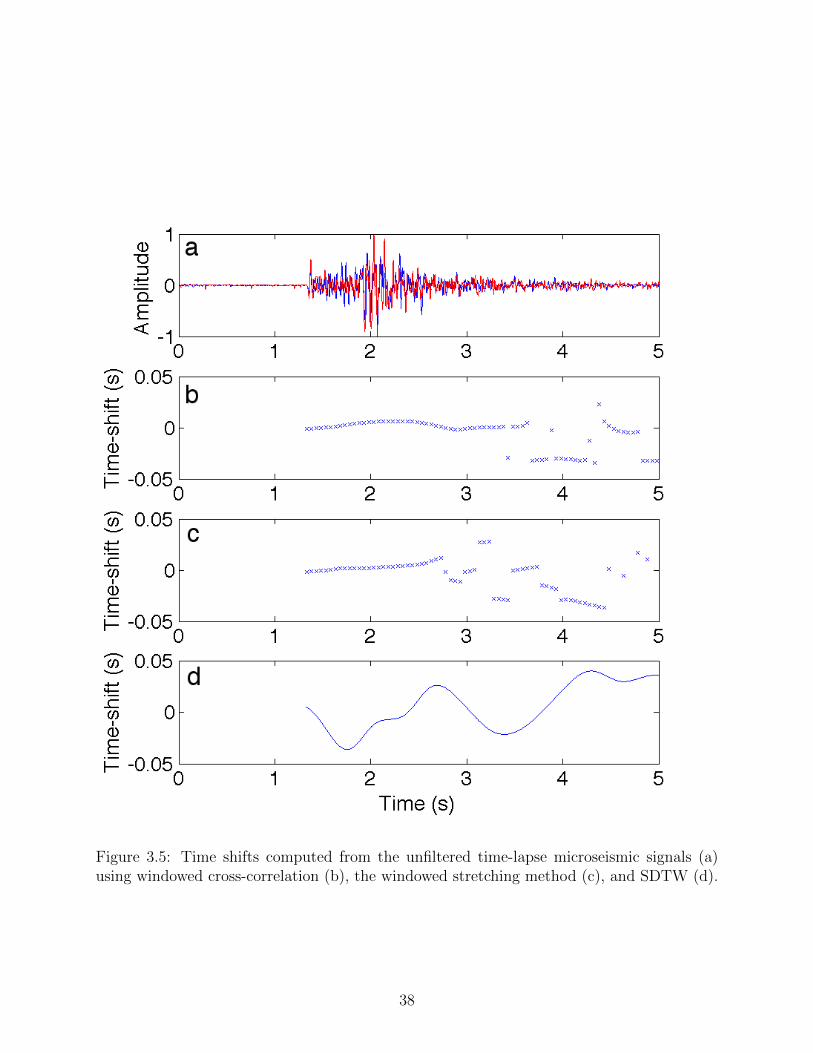
Figure 3.5: Time shifts computed from the unfiltered time-lapse microseismic signals (a)using windowed cross-correlation (b), the windowed stretching method (c), and SDTW (d).

38

Figure 3.6: Time shifts computed from the 5-15Hz bandpassed time-lapse microseismic sig-nals (a) using windowed cross-correlation (b), the windowed stretching method (c), andSDTW (d).

39

the SDTW estimates, especially at times with high signal-to-noise ratios. This is due to an

averaging e↵ect of the windowing. Late in the coda, for example at t > 3.5 s, the windowed

cross-correlation and stretching method show more variability in time shifts compared to the

early coda. This variability in the late coda is due to the low signal-to-noise ratio; this e↵ect

is also noted when computing time shifts using SDTW, as shown in Figure 3.5d. However,

the estimated time shifts using SDTW are more continuous. In Figure 3.5d and Figure 3.6d,

we bound �v/vo

to ±10%.

We also compute the time shifts using the filtered time-lapse signals shown in Figure 3.6a

to improve our time shift estimates. We filter the high frequency noise from the previously

shown time-lapse signals using a 5-15 Hz bandpass filter; this range spans the dominant

frequencies of the signal. Figure 3.6 shows estimates of time shifts from these filtered signals

using all three methods. These estimates contain smaller time shift variations compared

to the time shifts estimated from unfiltered recorded data shown in Figure 3.5. The time

shifts computed using SDTW show a larger variability with time compared to the time shifts

estimated from windowed cross-correlation and stretching method. The averaging e↵ect of

the time windowing of the time-lapse signals via the cross-correlation and stretching methods

reduces this variability of the time-shifts across the coda. The estimated time shifts from

these three methods are similar from t = 1 s to t = 2.7 s (Figure 3.6). For traveltimes

greater than 2.7 s, the SDTW estimated time shifts deviate from the estimated time shifts

that are computed using cross-correlation and stretching methods. The time shifts computed

using SDTW are dependent on the sampling of amplitude-aligned grid points and the du/dt

constraints used (equation 3.9).

From the time shifts, estimated using SDTW, we compute relative velocity changes using

equation 3.8, as shown in Figure 3.7. We vary these relative velocity changes by varying the

bounds on the maximum and minimum relative velocity change to: ±5%, ±10%, ±15%,

and ±20%. As shown in Figure 3.7b, if we vary these constraints, we also vary the resulting

relative velocity changes. When the signal to noise ratio is large, the relative velocity change

40

is consistent, as seen in early times in the signal. When the signal to noise ratio is low, the

relative velocity change varies more as we vary the constraints on �v/vo

. Figure 3.7 can be

used to measure the time-varying uncertainty of our relative velocity change estimation. The

red points shown in Figure 3.7a align with peaks and troughs of amplitudes in the signals.

These points correspond to the grid points used to coarsely sample time shifts in SDTW.

Notice a gap in grid points from 0 s to about 1 s; this is gap that we compute by measuring

the first arrival time among the time-lapse signals.

Figure 3.7: Relative velocity changes (b) computed from the 5-15Hz bandpassed time-lapsemicroseismic signals (a) using SDTW and multiple bounds on du/dt. Time shifts are sampledon an amplitude-aligned coarse grid (red points) (a).

3.5 Monitoring with downhole arrays

To compare the ability of these time shift estimation methods in identifying localized

velocity changes within the subsurface, we consider a synthetic example with a time-lapse

monitoring source (red) and receiver (blue) setup given in Figure 3.8a that shows both the

41

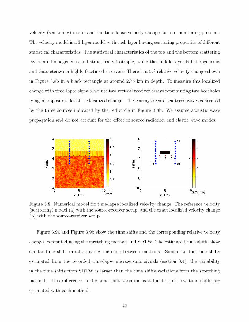
velocity (scattering) model and the time-lapse velocity change for our monitoring problem.

The velocity model is a 3-layer model with each layer having scattering properties of di↵erent

statistical characteristics. The statistical characteristics of the top and the bottom scattering

layers are homogeneous and structurally isotropic, while the middle layer is heterogeneous

and characterizes a highly fractured reservoir. There is a 5% relative velocity change shown

in Figure 3.8b in a black rectangle at around 2.75 km in depth. To measure this localized

change with time-lapse signals, we use two vertical receiver arrays representing two boreholes

lying on opposite sides of the localized change. These arrays record scattered waves generated

by the three sources indicated by the red circle in Figure 3.8b. We assume acoustic wave

propagation and do not account for the e↵ect of source radiation and elastic wave modes.

Figure 3.8: Numerical model for time-lapse localized velocity change. The reference velocity(scattering) model (a) with the source-receiver setup, and the exact localized velocity change(b) with the source-receiver setup.

Figure 3.9a and Figure 3.9b show the time shifts and the corresponding relative velocity

changes computed using the stretching method and SDTW. The estimated time shifts show

similar time shift variation along the coda between methods. Similar to the time shifts

estimated from the recorded time-lapse microseismic signals (section 3.4), the variability

in the time shifts from SDTW is larger than the time shifts variations from the stretching

method. This di↵erence in the time shift variation is a function of how time shifts are

estimated with each method.

42

Figure 3.9: A comparison of the estimated time shifts (a) and relative velocity changes (b)using stretching method (black) and smooth dynamic warping (red). These timeshifts andvelocity changes are estimated using the time-lapse signals for Source 2 and Receiver 3 pairshown in Figure 3.8.

Time shifts computed using STDW vary more with time compared to the windowed

stretching method. Figure 3.9b also shows the time-varying relative velocity changes com-

puted using SDTW and stretching method; SDTW shows more variability in the relative

velocity change with time. This estimated velocity change is a fraction of the true velocity

change, where the fraction depends on the relative time the scattered wave spends in the

region of change relative to the traveltime of the scattered wave [75].

Figure 3.10 shows source-receiver estimated time shifts relative to the location of the

velocity change both in the early and late coda. Both time shift estimation methods give

similar source-receiver distribution of the time shifts. Early in the coda waves (near t = 1.6 s

in Figure 3.10a), the estimated time shifts are larger for source-receiver paths that intersect

the localized velocity change. This distribution of time shifts in the early coda is also reflected

in the estimated velocity changes shown in Figure 3.11. Relative velocity changes computed

using SDTW are a better indicator of the magnitude localized velocity change in our model

than the relative velocity changes computed using the stretching method but the estimated

relative velocity change using SDTW suggests negative velocity change which is not present

in the time-lapse model.

Later in the coda (near t = 3.4 s in Figure 3.10a), the time shifts average across the source-

receiver pairs such that the source-receiver pairs below the region of change are a↵ected by

43

the localized change. This behavior of the time shifts in the late coda results from scattered

waves that travel along paths other than the direct source-to-receiver path. We need the

statistical properties of the scattering model to understand the behavior of the time shifts and

the scattered waves late in the coda. For more details on the behavior of the scattered waves

in a random scattering medium, we refer the reader to Kanu and Snieder [38]. However,

the time shifts in the early coda give a preliminary indication of the location of the velocity

change.

3.6 Conclusion

In this paper, we compare time shift and relative velocity change estimations using three

methods: time shift cross-correlation, stretching method, and smooth dynamic time warping

(SDTW). We compare these methods using both synthetic time-lapse signals and recorded

time-lapse microseismic signals. The synthetic signals allow for a comparison of the results

of the three methods with known exact values, while the recorded microseismic signals allow

us to compare the methods in the presence of noise.

Compared to the time shift cross-correlation and the stretching method, time shifts com-

puted using SDTW are more detailed. This is because the SDTW time shifts are computed

by optimally aligning two signals. In the time shift cross-correlation and stretching methods,

the time shifts and relative velocity changes are estimated within windows. This leads to an

averaging of the estimated time shift or velocity change values within the time window, which

smooths the variations in the time shifts. However, the averaging by the cross-correlation

and stretching methods reduces the impact of signal noise on the time-shift estimations.

SDTW may be inaccurate in the presence of noise if time shifts are computed on a finely

sampled grid, but if we use an amplitude-aligned coarse grid, the e↵ect of noise on the result-

ing time shifts is reduced. We are also able to constrain relative velocity changes by imposing

constraints on du/dt, thus further limiting potential errors in our time shifts due to noise.

We use the amplitude-aligned grid points and constraints on relative velocity changes that

minimize the e↵ect of noise and provide an optimal tie of the time-lapse signals. SDTW

44

Figure 3.10: The early (near t = 1.6 s) and late (near t = 3.4 s) coda of the time-lapsesignals (a) are highlighted. Time shifts from the early coda are computed using the stretchingmethod (b) and SDTW (c), and time shifts in the late coda are also computed using thestretching method (d) and SDTW (e). The colored lines indicate the magnitude of theestimated traveltime changes.

45

Figure 3.11: Distribution of the relative velocity changes between time-lapse signals com-puted using the stretching method (a) and SDTW (b) among source-receiver pairs. Thevelocity changes are estimated using the early part of the time-lapse coda. Blue circles arethe receivers while the red circles are the sources. The blue rectangle gives the localizedtime-lapse velocity change of 5%. The colored lines indicate the magnitude of the estimatedrelative velocity changes.

is also una↵ected by cycle-skipping, which causes errors in estimating time shifts using the

cross-correlation method.

3.7 Acknowledgments

We thank the sponsors of the Consortium Project on Seismic Inverse Methods for Com-

plex Structures, whose support made this research possible. We are also grateful to Roel

Snieder for initiating the idea of this study, his helpful suggestions, and his witty jokes.

46

CHAPTER 4

NUMERICAL COMPUTATION OF THE SENSITIVITY KERNEL FOR TIME-LAPSE

MONITORING WITH MULTIPLY SCATTERED ACOUSTIC WAVES

Chinaemerem Kanu and Roel Snieder

To be submitted to Geophysical Journal International (2015)

4.1 Abstract

In time-lapse monitoring of weak localized changes within a medium using coda waves,

we can either use the resulting decorrelation and/or the phase shift of the coda waves. The

formulation for both the decorrelation and the phase-shift of the coda waves resulting from

the weak time-lapse changes contains a common sensitivity kernel that is needed to image

the weak localized changes. We provide a novel approach to compute the sensitivity kernel

which uses numerical modeling (finite di↵erence) of the wavefields from the source and the

receiver with an a priori scattering model. These wavefields give the intensities needed

to compute the sensitivity kernels. This approach is di↵erent from common methods of

computing the sensitivity kernel that use analytical approximations of the scattered intensity.

The numerical solution of the sensitivity kernel allows us to use arbitrary earth model that

may include a free surface without simplifying the property of the scattering model. We

demonstrate the behavior of the numerical solution of the sensitivity kernel with end members

of heterogeneous scattering models.

4.2 Introduction

Multiple scattering of seismic waves along their travel paths potentially provides informa-

tion about the subsurface that can be used to increase the resolution of an imaged subsurface

(with multiple reflected waves) [8], increase illumination especially within a poorly illumi-

nated subsurface [26, 28] and monitor weak time-lapse changes within the earth’s subsurface

47

[76, 87, 97]. Using scattered waves, especially for monitoring temporal weak changes within

the subsurface, we can increase the illumination and resolution of time-lapse changes within

a subsurface [10, 52]. Multiply scattered waves are used for monitoring weak changes such as

velocity changes as weak as 0.1% [97] and monitoring defects within mechanical structures

[55]. However, the complexity in the travel paths of the multiply scattered waves, which

depends on the scattering properties of the medium of interest, makes it challenging to ac-

curately describe the origin, travel paths, and distribution of the scattered waves within the

medium. In a strongly scattering medium, the multiply scattered waves for late lapse time

can be described as a di↵usive process [72, 92, 112]. The di↵usion model has been used suc-

cessfully in imaging algorithms that use multiply scattered waves in medical imaging [113] or

in imaging of missing scatterers [82]. But, the validity of using the di↵usion intensity model

in explaining the multiple scattering of waves depends on the strength of the scattering pro-

cess. Even in a strongly scattering medium, the di↵usion intensity model is only accurate at

large lapse times, i.e. for t >> r/c, where t is the travel-time, r is the source-receiver dis-

tance and c is the average velocity of the medium. Alternatively, the scattered intensity can

be modeled using the radiative transfer intensity model, which more accurately predicts the

scattered intensity for all scattering regimes [69, 105]. The di↵usion and radiative transfer

intensity models are analytical models developed under the assumption of a stochastic wave

equation. These analytical intensity models, as well as most other intensity models for the

scattered waves, are based on homogeneous or simple scattering media. The scattered inten-

sity can easily become complicated if the statistical properties of the scattering medium are

heterogeneous. We show that for more realistic media, a more accurate scattered intensity

can be modeled numerically using, for example, finite-di↵erence modeling rather than using

the analytical intensity models.

Time-lapse changes within the earth’s subsurface (both natural and induced) are usually

either gradual, weak, or localized both in space and time. Detecting these changes in many

cases requires data that are highly sensitive to the changes. Vlastos et al. [108] show that

48

the sensitivity of multiply scattered waves to the weak changes is significantly higher than

the sensitivity of the ballistic or direct part of the seismic waves to the weak changes. This

increase in the sensitivity is due to the repeated sampling of the weak velocity changes by the

scattered waves [81]. The high sensitivity of the multiply scattered waves has led to successful

detection of time-lapse velocity changes within the earth’s subsurface. Poupinet et al. [76] use

coda waves generated by repeating earthquakes to observe an average S wave velocity change

of 0.2% after the 1979 Mw

5.9 Coyote Lake earthquake on the Calaveras Fault, California.

Using correlation functions generated from seismic noise, Wegler and Sens-Schonfelder [111]

detect a sudden decrease in the seismic velocity of the region surrounding the 2004 Mw

6.6

Mid-Niigata earthquake rupture. Using controlled-source monitoring Nishimura et al. [64]

detected a velocity decrease of 0.3-1.0 % due to the 1998 Mw

6.1 Mount Iwate earthquake.

However, Pacheco and Snieder [70] show that the spatial sensitivity of the multiply scattered

waves to the time lapse changes is not uniformly distributed but is dependent on the source

and receiver locations.

Most time-lapse monitoring of weak changes within the earth’s subsurface using multiply

scattered waves has been limited to identifying weak changes rather than localizing these

changes. Except in very densely distributed source and receiver set-ups, the velocity changes

detected by coda wave interferometry are spatially averaged velocity changes. Recently,

successful e↵orts have been made not only in identifying the weak changes using multiply

scattered waves, but also in localizing the changes in a statistically homogeneous scattering

medium [82]. However, to localize changes within the earth’s subsurface - a scattering

medium which is most likely to be inhomogenous - we will need to appropriately handle the

inhomogeneities of the earth’s subsurface. Because of the prominence of surface waves, we

also need to account for the presence of a free surface.

In this study, we explore the capability of computing the sensitivity kernel that we need

for time-lapse monitoring and localizing the weak changes within a medium. In the next

subsection, we describe the theoretical connection of the sensitivity kernel to the estimated

49

time lapse time-shifts or the decorrelations in the time lapse scattered waves resulting from

the weak changes. In section 4.4, we develop a novel approach for computing the kernel

numerically for any scattering model and explore the behavior of the kernel using various

end-member scattering models. In section 4.5, we discuss the practicality of the kernel

computation.

4.3 Sensitivity Kernel

Pacheco and Snieder [70] use the intensity of multiply scattered waves to develop a

sensitivity kernelK(s,xo

, r, t) which relates the mean travel time changes h⌧i to the localized

relative velocity change within the subsurface �v/v(xo

):

h⌧(t)i = �Z

V

K(s,xo

, r, t)�v

v(x

o

) dV (xo

), (4.1)

where t is the travel-time of the scattered wave, V is the scattering volume, and s and r

are the source and the receiver locations, respectively. The sensitivity kernel K(s,xo

, r, t)

depends on the source and receiver locations, the scattering property of the medium, and

the travel-time of the scattered wave.

Rossetto et al. [82] consider a di↵erent problem where the local scattering strength

changes. This change is accounted for by a change in scattering cross-subsection ��(xo

).

Using the correlation function C(s, r, t) of the multiply scattered waves in a medium with

this time-lapse change, they relate the decorrelation 1�C(s, r, t) of the time lapse scattered

waves to the time lapse change in the total scattering cross-subsection of the medium:

1� C(s, r, t) =

Z

V

v(xo

)��(xo

)

2K(s,x

o

, r, t) dV (xo

). (4.2)

Using either the time-shifts or the decorrelation values from the time-lapse multiply

scattered waves for resolving localized weak changes, the sensitivity kernelK(s,xo

, r, t) forms

the building block for the Frechet derivatives needed to resolve the weak changes. The

50

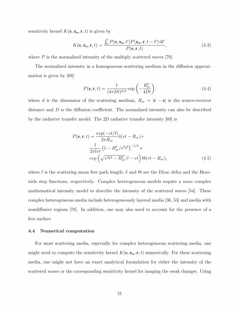
sensitivity kernel K(s,xo

, r, t) is given by

K(s,xo

, r, t) =

Rt

0 P (s,xo

, t0)P (xo

, r, t� t0) dt0

P (s, r, t), (4.3)

where P is the normalized intensity of the multiply scattered waves [70].

The normalized intensity in a homogeneous scattering medium in the di↵usion approxi-

mation is given by [69]:

P (s, r, t) =1

(4⇡Dt)d/2exp

✓�R2

sr

4Dt

◆, (4.4)

where d is the dimension of the scattering medium, Rsr

= |r � s| is the source-receiver

distance and D is the di↵usion coe�cient. The normalized intensity can also be described

by the radiative transfer model. The 2D radiative transfer intensity [69] is

P (s, r, t) =exp(�vt/l)

2⇡Rsr

�(vt�Rsr

)+

1

2⇡lvt

�1�R2

sr

/v2t2��1/2 ⇥

exp⇣p

v2t2 �R2sr

/l � vt⌘⇥(vt�R

sr

), (4.5)

where l is the scattering mean free path length; � and ⇥ are the Dirac delta and the Heav-

iside step functions, respectively. Complex heterogeneous models require a more complex

mathematical intensity model to describe the intensity of the scattered waves [54]. These

complex heterogeneous media include heterogeneously layered media [36, 53] and media with

nondi↵usive regions [78]. In addition, one may also need to account for the presence of a

free surface.

4.4 Numerical computation

For most scattering media, especially for complex heterogeneous scattering media, one

might need to compute the sensitivity kernel K(s,xo

, r, t) numerically. For these scattering

media, one might not have an exact analytical formulation for either the intensity of the

scattered waves or the corresponding sensitivity kernel for imaging the weak changes. Using

51

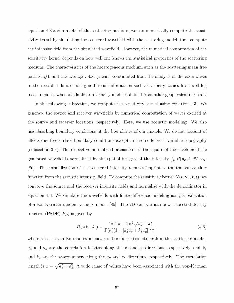
equation 4.3 and a model of the scattering medium, we can numerically compute the sensi-

tivity kernel by simulating the scattered wavefield with the scattering model, then compute

the intensity field from the simulated wavefield. However, the numerical computation of the

sensitivity kernel depends on how well one knows the statistical properties of the scattering

medium. The characteristics of the heterogeneous medium, such as the scattering mean free

path length and the average velocity, can be estimated from the analysis of the coda waves

in the recorded data or using additional information such as velocity values from well log

measurements when available or a velocity model obtained from other geophysical methods.

In the following subsection, we compute the sensitivity kernel using equation 4.3. We

generate the source and receiver wavefields by numerical computation of waves excited at

the source and receiver locations, respectively. Here, we use acoustic modeling. We also

use absorbing boundary conditions at the boundaries of our models. We do not account of

e↵ects due free-surface boundary conditions except in the model with variable topography

(subsection 3.3). The respective normalized intensities are the square of the envelope of the

generated wavefields normalized by the spatial integral of the intensityRV

P (xo

, t) dV (xo

)

[86]. The normalization of the scattered intensity removes imprint of the the source time

function from the acoustic intensity field. To compute the sensitivity kernel K(s,xo

, r, t), we

convolve the source and the receiver intensity fields and normalize with the denominator in

equation 4.3. We simulate the wavefields with finite di↵erence modeling using a realization

of a von-Karman random velocity model [86]. The 2D von-Karman power spectral density

function (PSDF) P2D is given by

P2D(kx, kz) =4⇡�(+ 1)✏2

pa2x

+ a2z

�()(1 + [k2x

a2x

+ k2z

a2z

])+1, (4.6)

where is the von-Karman exponent, ✏ is the fluctuation strength of the scattering model,

ax

and az

are the correlation lengths along the x- and z- directions, respectively, and kx

and kz

are the wavenumbers along the x- and z- directions, respectively. The correlation

length is a =p

a2x

+ a2z

. A wide range of values have been associated with the von-Karman

52

parameters for the earth subsurface. The values of the von-Karman parameters depend on

the subsurface lithology and the depth of the subsurface. Using the autocorrelation function

of surface rock samples from Westerly and Oshima granite, Spetzler et al. [101] estimate for

the Westerly granite ✏ = 8.5 % and a = 0.22 mm while ✏ = 9.3 % and a = 0.46 mm for the

Oshima granite. Yoshimoto and Sato [114], using 149 waveforms in the frequency band of 8

- 16 Hz from 10 earthquakes occurring at depths shallower than 10 km, estimates the range

of ✏ and a values to be 5 - 8 % and 0.3 - 0.8 km, respectively, in the Nilko area of Japan.

The scattering model we use for kernel computation consists of the random velocity

fluctuations defined by the von-Karman parameters and constant density. The velocity

model is given as

v(x) = v0(x)[1 + ⇣(x)], (4.7)

where v0(x) is the background velocity and ⇣(x) is a realization of the random velocity

fluctuation for the von-Karman PSDF in equation 4.6 [86].

4.4.1 Numerical vs. analytical computation

The sensitivity kernel can be estimated from analytical models of the scattered intensity

(the di↵usion and radiative transfer approximation of the scattered intensity). To compare

the analytical and numerical solution of the sensitivity kernel, we use a von-Karman scat-

tering model defined by the following parameters: ax

= ay

= 0.01 km, ✏ = 0.1, = 0.5, and

f = 15 Hz (� = 0.23 km). This scattering model and the dominant scattering wavenumber

correspond to ka ' 0.27. The scattering velocity model is given in Figure 4.1 with an average

velocity of 3.5 km/s. The theoretical scattering mean free path length (lV K

) and transport

mean free path length (l⇤V K

) for these von-Karman parameters and the scattered waves are

5.7 km and 6.9 km, respectively [86].

We compute the analytical solution of the sensitivity kernel by using the corresponding

theoretical mean free path lengths and the approximations of the scattered intensity using the

di↵usion (equation 4.4) and the radiative transfer (equation 4.5) models. We also convolve

53

0 2 4 6 8 104.44.24.0

3.83.63.43.2

02

46

810

x (km)

z (k

m)

3.0

2.82.6

km/s

Figure 4.1: Velocity model for numerical computation of sensitivity kernel for comparisonwith the analytical solution.

Figure 4.2: Temporal and spatial evolution of the sensitivity kernel (numerical solution).

54

Figure 4.3: Temporal and spatial evolution of the sensitivity kernel using the radiativetransfer model.

55

Figure 4.4: Temporal and spatial evolution of the sensitivity kernel using the di↵usion model.

56

the analytical intensities with the intensity of the source wavelet used for the computation

of the numerical kernel. Figure 4.2, Figure 4.3 and Figure 4.4 show time snapshots of

the temporal evolution of the sensitivity kernel for both the numerical and the analytical

solutions, respectively. In Figure 4.2, Figure 4.3 and Figure 4.4, the time-shots are taken at

0.95 s, 1.20 s, 2.00 s, and 4.00 s. The numerical solution of the sensitivity kernel is bound by

the a kernel front which is defined as the edge of the kernel that is dominantly composed of

single scattering and bounds the multiple scattering contributions. The numerical sensitivity

kernel shows similar features represented in the radiative transfer model (Figure 4.3) of the

sensitivity kernel including the direct line-of-sight characteristic of the ballistic kernel (0.95

s) and the elliptical shape of the kernel front at lapse times after the first arrival time.

The major di↵erence between the numerical kernel and the radiative transfer kernel is the

fluctuations in the numerical kernel. The numerical kernel in Figure 4.2 is computed with one

realization of the scattering model. These kernel fluctuations are suppressed by averaging the

numerical kernel over many realizations of the scattering model. The di↵usion approximation

of the sensitivity kernel (Figure 4.4), as expected, only reproduces the spatial features of the

kernel at long lapse times (ct/Rsr

� 1) [69] with no clear ellipsoidal edge. Figure 4.5 shows

a cross-subsection of the kernel along the source-receiver line. The di↵usion kernel fails to

explain the zero or near-zero sensitivity of the kernel beyond the kernel front, evident in

both the numerical and the radiative transfer kernels.

The spatial and temporal behavior of the kernel implies that to resolve time-lapse changes

within a scattering medium with homogeneous statistical properties, the radiative transfer

kernel can closely substitute for the numerical kernel solution. Figure 4.5 shows that the

numerical kernel has more fluctuations compared to the analytical solutions. This numerical

kernel is computed with one realization of the scattering model. The kernel fluctuations

which are due to isolated scatterers within the scattering model, are present in the multiply

scattering contribution to the kernel. We can suppress the kernel fluctuations by averaging

the kernel over a number of the realizations of the scattering model with the same statistical

57

properties. Figure 4.6 shows the averaged kernel at travel-time 2.00 s over 1, 5, 10 and 20

realizations of the scattering model. Increasing the number of realizations of the model used

for the kernel computation reduces the fluctuations both at the singly scattered and multiply

scattered part of the kernel. With few realizations of the random model (5-10 realizations)

we can achieve stability in the sensitivity kernel (Figure 4.7).

4.4.2 Scattering Velocity models

Random isotropic scattering model

Figure 4.2 shows the kernel for a given source-receiver pair (S-R) at the following time

snapshots: 0.95 s, 1.20 s, 2.00 s, and 4.00 s. The direct wave excited by a source S arrives

at the receiver R at travel-time t = 0.90 s with an average velocity of 3.5 km/s. The

time snapshots of the kernel shown in Figure 4.2 show the sensitivity to the changes in the

scattering model for the scattered phases arriving at a specific travel-time t. The kernel at t

= 0.95 s corresponds to the sensitivity of scattered waves dominated by direct and forward

scattered waves. With increasing time, the area covered by the sensitivity kernel progressively

increases. The spatial broadening of the kernel with time increases the detectability of any

change in the scattering property of the medium due to multiple interaction between the

scattered waves and the change with time, especially changes away from the path of the direct

wave (which is along the source-receiver line in this case). However, the resolving power of

the kernel is expected to decrease with increasing time because of the spatial broadening of

the kernel. The shape of the kernel with increasing time depends on the source and receiver

locations, the corresponding travel-time, and the properties of the scattering medium. At

times t > 0.95 s, the kernel assumes an elliptical shape with the major axes along the

source-receiver line and the minor axes perpendicular to the source-receiver line. The edge

of the kernel is dominated by contributions from single scattering. The kernel for the singly

scattered waves is given by [71]

K(xo

, t) =1

2⇡hp

(ct/Rsr

� 1)

hrs

s+

rr

r

i, (4.8)

58

where s and r are the distances from the point xo

to the source and receiver, respectively;

rs

and rr

are the distances from any point on the kernel front to the source and receiver,

respectively.

Figure 4.5: Comparison between numerical sensitivity kernel (black line) and di↵usion- (blueline) and radiative transfer- (red line) based kernel along the source- (at 2 km) receiver- (at5 km) line.

The single-scattering-dominated part of the kernel spatially bounds the multiple scat-

tering part of the kernel. The inner part of the kernel accounts for multiple scattering,

which has lower amplitude compared to the kernel contribution from the single scattering.

Within the multiple-scattering-dominated part of the kernel, there are high sensitivities at

59

Figure 4.6: Compassion of the kernel at t = 2.0 s using a number of scattering modelrealizations

60

the source and receiver locations which are predicted accurately by the analytical solutions

in Figure 4.5. These high sensitivities at or near the source and receiver locations suggest

that the dominant contribution to the multiply scattered waves recorded at receiver R due

to a source S originates from scattering near the source and receiver locations.

0 5 100

1

2

3

4

5

6

7x10

−7

x (km)

Sensitivity

kernel(s/m

)

151020

0 5 100

1

2

3

4

5

6

7x10

−7

z (km)

Sensitivity

kernel(s/m

)

151020

2

0 5 100

1

2

3

4

5

6

7x10

−7

x (km)

Sensitivity

kernel(s/m

)

151020

0 5 100

1

2

3

4

5

6

7x10

−7

z (km)

Sensitivity

kernel(s/m

)

151020

2

0 5 100

1

2

3

4

5

6

7x10

−7

x (km)

Sensitivity

kernel(s/m

)

151020

0 5 100

1

2

3

4

5

6

7x10

−7

z (km)

Sensitivity

kernel(s/m

)

151020

2

0 5 100

1

2

3

4

5

6

7x10

−7

x (km)

Sensitivity

kernel(s/m

)

151020

0 5 100

1

2

3

4

5

6

7x10

−7

z (km)

Sensitivity

kernel(s/m

)

151020

2 2

A B

Figure 4.7: The inline subsection (A) and the crossline subsection (B) of the kernel at t = 2.0s after averaging over 1, 5, 10, and 20 realizations of the scattering model with the samestatistical properties.

Random non-isotropic scattering model

The scattering properties within the earth’s subsurface are generally complex and inho-

mogeneous. The scattering characteristics of the subsurface can vary from place to place

depending on both the underlying lithology and overlaying stress conditions of the local and

regional subsurface. The scattering properties of the earth’s subsurface also vary with depth

[93]. The stress- and depth- dependent scattering properties of the subsurface controls the

scattering process of the seismic wave traveling through the subsurface. The e↵ective scat-

tering of the subsurface are defined by both the scattering properties of the subsurface and

the characteristics of the incident seismic phase that is scattered. The characteristics of the

incident phase include the incidence angle of the wave, the spectral properties of the incident

wave, and the wave mode of the incident wave [45].

61

To explore the dependence of the sensitivity kernel on the scattering medium, we test two

scattering models whose background velocity is a 3-layered velocity model. In both models

(Figure 4.8 and Figure 4.11), the top and bottom layers have the same scattering properties

given by the von-Karman PSDF. For the top layer, = 0.5, ✏ = 0.5, and az

= ax

= 0.05 km;

for the bottom layer, = 0.8, ✏ = 0.1, and az

= ax

= 0.1 km. However, in the middle layer,

one model consists of vertical velocity perturbations while the other model is composed of

horizontal velocity perturbations. The model with vertical velocity perturbations mimics a

highly vertically fractured reservoir while the model with horizontal velocity perturbations

represents a shale-like reservoir with a thin laminated layering. The middle layer for both

models is defined by the following von-Karman parameters. For the vertically fractured

model, az

= 0.5 km and ax

= 0.0001 km; for the shale-like model, az

= 0.0001 km and ax

= 0.5 km. In both models, = 0.1 and ✏ = 0.5 for the middle layer. In both scattering

models, we compute the sensitivity kernels using two source-receiver configurations. In one

configuration, the source-receiver line is vertical while in the second configuration the source-

receiver line is horizontal and is embedded within the middle layer. These source-receiver

configurations resemble a source such as a microseismic event or an earthquake embedded

within the subsurface with either a receiver at the near surface (for the vertical source-receiver

line) or a receiver within a borehole (for the horizontal source-receiver line).

Figure 4.9 and Figure 4.10 give time snapshots of the sensitivity kernel in the vertically

fractured model for the vertical and horizontal source-receiver configurations, respectively.

In both source-receiver configurations, the kernels show many of the features present in the

kernel of the random isotropic model (Figure 4.2), which include the spatial broadening of the

kernel with increasing time, the high sensitivity at the source and receiver locations, and the

presence of the single scattering contributions to the kernel at the kernel front. However, the

heterogeneity in the scattering model introduces extra features to the kernel of the vertically

fractured model which are not present in the random isotropic kernel (Figure 4.2). In both

source-receiver configurations, the width of the kernel (along the minor axes of the kernel)

62

at each layer of the model depends on the e↵ective velocity in that layer (see Figure 4.9

and Figure 4.10 at t = 2.50 s). In the vertical source-receiver configuration at t = 2.50 s

and 5.00 s, there are extra scattered fronts marked as S00within the kernel; these fronts are

secondary scattered intensity fronts due to reflections from the layer interfaces in the model.

These reflected fronts lag behind the singly scattered front. In the horizontal source-receiver

configuration (Figure 4.10), the direct wave refracts through the top interface of the bottom

layer because of the higher velocity of the bottom layer (Figure 4.10 at t = 1.38 s). A

few milliseconds later, many of the forward scattered waves are confined within the middle

layer (Figure 4.10 at t = 1.40 s). At later lapse times, the singly scattered kernel front

propagates out from the middle layer into the top and the bottom layers. The extent of the

front propagation depends on the average velocity of the layer. The reflected wavefronts S00

seen in the vertical source-receiver configuration are absent in the kernel with the horizontal

source-receiver configuration. This is because the reflectors are parallel to the source-receiver

line in the horizontal configuration. The sensitivity is dominant within the middle layer

because the vertical velocity perturbations within the middle layer persistently reflects back

and forth waves traveling horizontally between the source and the receiver. The orientations

of the velocity perturbations are perpendicular to the dominant forward propagation of the

waves which is along the source-receiver line (Figure 4.10 at t = 2.50 s and 5.00 s). This

dominance of the kernel in the middle layer is not present with the vertical source-receiver

setup (Figure 4.9), where in the middle layer the wave propagation direction is along the

direction of the velocity perturbation. The lack of the kernel dominance within the middle

layer with a vertical source-receiver setup is because of the relative orientation of the source-

receiver line and the orientation of the scatterers which results to minimal scattering of the

waves compared to the horizontal source-receiver setup. Also the scattered waves recorded

at the receiver has a higher probability of exploring the whole model space without being

trapped within middle layer due to scattering. With the horizontal source-receiver setup,

much of the recorded scattered waves are generated within the middle layer.

63

0 2 4 6 8 104.4

4.0

3.6

3.2

2.8

2.4

2.0

02

46

810

x (km)

z (k

m)

km/s

Figure 4.8: Velocity model with a vertical-fractured-like reservoir.

Figure 4.12 and Figure 4.13 give time snapshots of the sensitivity kernel in the shale-

like model using the vertical and horizontal source-receiver configurations, respectively. The

kernel for the shale-like model, which uses a vertical source-receiver configuration, exhibits

similar features present in the vertically fractured model with a similar source-receiver setup.

Di↵erences in the kernels are in the multiply scattered part of the kernel in the middle

layer of the vertically fractured model where there are more scattering close to the source.

However, with the horizontal source-receiver configuration (Figure 4.13), the kernel at late

lapse time (t = 2.50 s and 5.00 s) shows features di↵erent from those present in the kernel

with the vertically fractured model using the horizontal source-receiver configuration. The

high sensitivity present in the vertically fractured model using the horizontal source-receiver

setup is absent from the model with the horizontal velocity perturbation in the middle layer

because the direction of wave propagation between the source and the receiver is parallel

to the velocity layering in the middle layer, which results in relatively less scattering of the

seismic wave. The e↵ect of the source-receiver setup on the kernel behavior implies that the

setup of the source and receiver pairs relative to the location of a particular time-lapse change

within a scattering medium has large implications for the capability of detecting and resolving

64

the time-lapse change. For example, if there is a change in the middle layer, the horizontal

source-receiver setup provides a better scenario for detecting and resolving the time-lapse

change in the middle layer than will the vertical source-receiver setup. This connection

between the source-receiver setup and the behavior of the sensitivity kernel suggests the

need for the source and receiver to be in close proximity to the location of the time-lapse

change. The relative direction of the forward scattering between the source and the receiver

to the orientation of the length of the scatterers impacts the relative magnitude of the

sensitivity of the scattered intensity to the time-lapse change. This impact is evident in a

comparison of the kernel strength in the middle layers of the vertically fractured model to

the kernel strength in the middle layer of the shale-like model. The relative strength of the

kernel is higher in the vertically fractured model where the perpendicular alignment of the

scatterers allows for a stronger generation of multiply scattered waves.

The kernels at early lapse times are almost identical in both models (Figure 4.9, Fig-

ure 4.10, Figure 4.12 and Figure 4.13 at t = 1.38 s and 1.40 s). The kernels at these times

consist of mainly direct, refracted, and forward scattered waves.

4.4.3 Topography-induced Scattering

Seismic waves are not only scattered by heterogeneities within the earth’s subsurface,

but also by near-surface heterogeneities such as variable topography or low velocity uncon-

solidated lithology in the near-surface layers. Due to the high impedance contrast across the

free surface and the higher heterogeneities within the near-surface compared to the hetero-

geneities deeper in the subsurface [93], the multiple scattering from variable topography and

near-surface scattering e↵ects can dominate bulk scattering. Rough or variable topography

plus the presence of the free surface can focus or defocus seismic waves and can convert

seismic waves from one wave mode to another such as conversion of body waves to surface

waves and vice versa [45]. Bouchon et al. [11] show that a simple symmetric ridge can induce

amplification of a monochromatic SH wave by up to a factor of 1.5 at the crest of the ridge.

The amplification factor of the incident wave depends on the incident angle of the wave and

65

0 2 4 6 8 10 x10-6

(s/m )202

46

810 0

0.5

1.0

x (km)

z (k

m)

R

S

t = 1.40s

0 2 4 6 8 10 x10-6

(s/m )202

46

810 0

0.5

1.0

x (km)

z (k

m)

R

St = 1.80s

0 2 4 6 8 10 x10-6

(s/m )202

46

810 0

0.6

0.2

0.4

x (km)

z (k

m)

R

S

S’’

S’’

t = 2.50s

0 2 4 6 8 10 x10-6

(s/m )202

46

810 0

1.0

2.0

0.5

1.5

x (km)

z (k

m)

R

St = 5.00s

Figure 4.9: Temporal and spatial evolution of the sensitivity kernel (numerical solution) ina reservoir with vertical-fractured-like velocity perturbation with a near-surface receiver. S 00

corresponds to the reflected scattered phase.

66

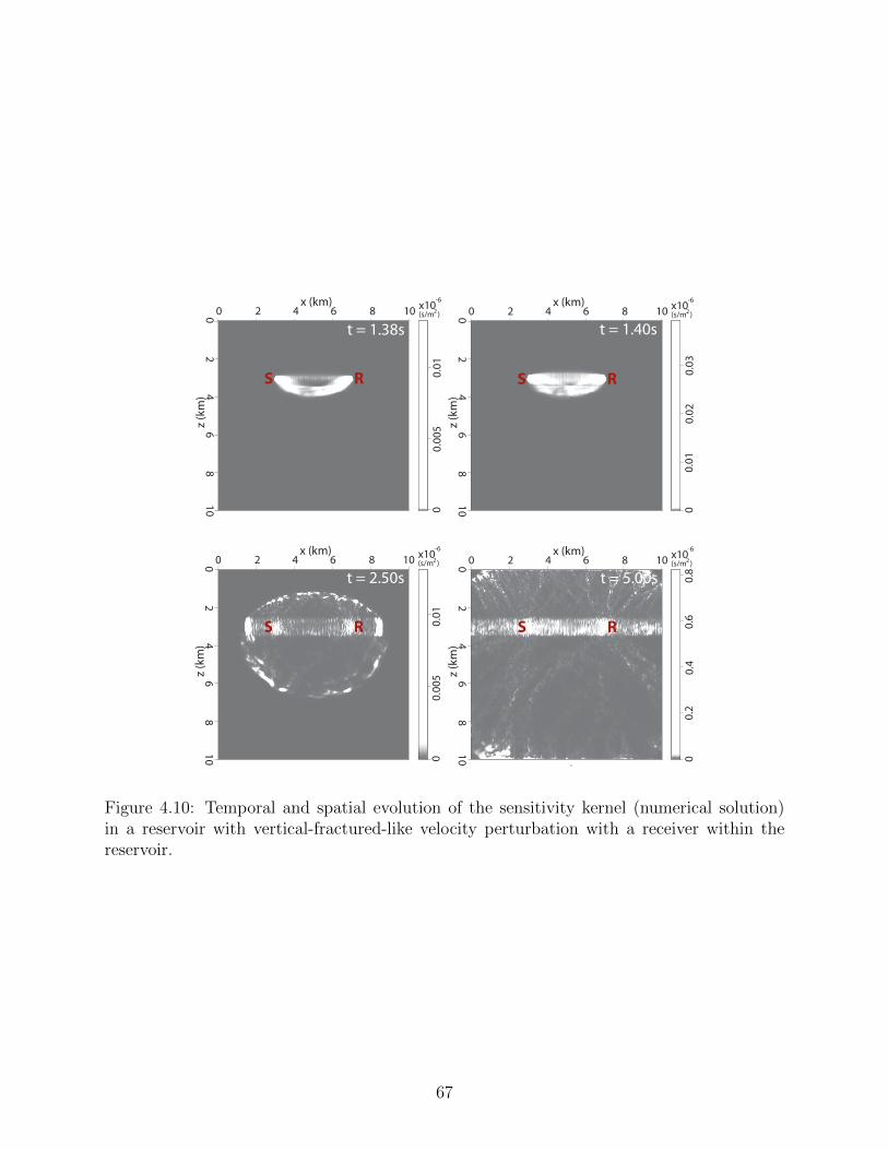
0 2 4 6 8 10 x10-6

(s/m )202

46

810 0

0.00

50.

01

x (km)

z (k

m)

t = 1.38s

RS

0 2 4 6 8 10 x10-6

(s/m )202

46

810 0

0.01

0.02

0.03

x (km)

z (k

m)

RS

t = 1.40s

0 2 4 6 8 10 x10-6

(s/m )202

46

810 0

0.00

50.

01

x (km)

z (k

m)

t = 2.50s

RS

0 2 4 6 8 10 x10-6

(s/m )202

46

810 0

0.2

0.4

0.6

0.8

x (km)

z (k

m)

t = 5.00s

RS

Figure 4.10: Temporal and spatial evolution of the sensitivity kernel (numerical solution)in a reservoir with vertical-fractured-like velocity perturbation with a receiver within thereservoir.

67

the height to width ratio of the topography perturbation.

0 2 4 6 8 104.4

4.0

3.6

3.2

2.8

2.4

2.0

02

46

810

x (km)

z (k

m)

km/s

Figure 4.11: Velocity model with a shale-like reservoir.

To explore the e↵ect of topography on the sensitivity kernel, we simulate an acoustic

wavefield using a homogeneous velocity model with a variable topography. The velocity

model consists of 3 homogeneous layers: a top air layer with a velocity of 330m/s, a thin

layer under the topography with a velocity of 2000 m/s, and the rest of the model with a

velocity of 3000 m/s (Figure 4.14). The free-surface is approximated using the air-subsurface

interface based on the velocity discontinuity assuming a constant density [103]. We model

the variable topography using a 1D von-Karman PSDF in order to create a random variable

topography with a correlation across the topography defined by a correlation distance of 0.5

km.

We compute the sensitivity kernel with the scattered waves induced by the variable to-

pography using a vertical source-receiver setup (Figure 4.15) and a horizontal source-receiver

setup (Figure 4.16). At time t = 1.40 s, the kernel accounts for the direct wave between

source S and receiver R. The direct wave kernel using the vertical source-receiver setup is

shown in Figure 4.15 at t = 1.40 s. At later lapse time (Figure 4.15; t > 1.40 s), the

kernel expands into a singly scattered front which broadens with time. The kernel has a

68

0 2 4 6 8 10 x10-6

(s/m )202

46

810 0

0.2

0.4

0.6

0.8

x (km)

z (k

m)

t = 1.40sR

S

0 2 4 6 8 10 x10-6

(s/m )202

46

810 0

24

68

x (km)

z (k

m)

t = 1.80sR

S

0 2 4 6 8 10 x10-6

(s/m )202

46

810 0

24

x (km)

z (k

m)

t = 2.50sR

S

S’’

S’’

0 2 4 6 8 10 x10-6

(s/m )202

46

810 0

24

6

x (km)

z (k

m)

t = 5.00sR

S

Figure 4.12: Temporal and spatial evolution of the sensitivity kernel (numerical solution) ina reservoir with shale-like velocity perturbation. S 00 corresponds to the reflected scatteredphase.

69

0 2 4 6 8 10 x10-6

(s/m )202

46

810 0

0.00

20.

004

0.00

60.

008

x (km)

z (k

m)

t = 1.38s

RS

0 2 4 6 8 10 x10-6

(s/m )202

46

810 0

0.01

0.02

x (km)

z (k

m)

t = 1.40s

RS

0 2 4 6 8 10 x10-6

(s/m )202

46

810 0

24

6

x (km)

z (k

m)

t = 2.50s

RS

0 2 4 6 8 10 x10-6

(s/m )202

46

810 0

510

x (km)

z (k

m)

t = 5.00s

RS

Figure 4.13: Temporal and spatial evolution of the sensitivity kernel (numerical solution) ina reservoir with shale-like velocity perturbation.

70

relatively large magnitude within the tiny low velocity layer underneath the topography

(Figure 4.15, t = 2.5 s and 5.0 s). This part of the kernel is due to scattering contributions

from the topography-induced scattering which are trapped in the near-surface layer. This

topography-induced sensitivity is contained predominantly within the near-surface layer by

the velocity interface on top of the high velocity halfspace. The topography-induced sensitiv-

ity, however, increases and broadens away from the receiver location within the near-surface

layer with an increase in time.

When the source and receiver are embedded within the near-surface layer underneath

the variable topography, the kernel of the first arrival consists of refracted waves o↵ of the

higher velocity halfspace underneath the near-surface low velocity layer (Figure 4.16, t =

1.6 s). Similar to the vertical source and receiver setup, the direct/refracted kernel with the

horizontal source and receiver setup splits for t= 1.8 s into the singly scattered kernel. In

Figure 4.16, only the downward subsection of the singly scattered kernel is present because

the high velocity contrast across the topography prevents propagation of scattered waves

into the air. At later lapse time (t = 2.50 s and 5.00 s, Figure 4.16), the dominant part

of the kernel lies within the low velocity layer which results from the topography-induced

scattering and the trapped waves within the low velocity layer. The presence of the thin

low velocity layer underneath the topography induces kernels with similar behavior at large

lapse time for both source-receiver setups.

The behavior of the kernel in the presence of variable topography and a thin low velocity

layer in the above results demonstrates the need to accurately characterize the scattering

properties of the medium being monitored. Incorporating both the topography and the

appropriate velocity (scattering) model in the kernel computation provides the distribution

and origin of the scattered waves via the kernel that can be used for time-lapse monitoring.

Due to the e↵ect of variable topography and of a heterogeneous scattering medium on the

kernel, we will need to use an appropriate source-receiver array setup to image a time-lapse

change within the subsurface. For example, in a case of monitoring velocity changes within

71

a reservoir that might be due to fluid production or injection within the reservoir, a borehole

array in close proximity to the change might be a more e↵ective source-receiver setup for

monitoring than using a surface-receiver array. In this case, the borehole array records more

of the scattered waves generated within a given layer. This results in higher sensitivity to

a change in that layer. Also, the borehole array, depending on its relative depth to the

free-surface, will have less of the topography- or near-surface- induced scattering.


We propose a novel approach to compute the sensitivity kernel that can be used to resolve

weak changes within the earth’s subsurface or any other medium using multiply scattered

waves. These are changes which are usually irresolvable with singly scattered waves. Our

approach does not rely on analytical models of the scattered intensity such as the di↵usion

and radiative transfer models. To compute the sensitivity kernel, we compute the scattered

intensity field needed for the kernel computation using an a priori model of the scattering

medium from numerically generated scattered wavefield. In this paper, we use the finite-

di↵erence modeling for the computation of the seismic wavefield. The numerical modeling of

the scattered intensity can take advantage of various numerical methods for seismic wavefield

computation. Using our approach we can incorporate any complexities of the scattering

medium and any boundary conditions of the medium. With an appropriate a priori scattering

model, we can obtain a more accurate estimate of the sensitivity kernel which accurately

describes the intensity of the scattered wave recorded by a given source-receiver pair. Our

kernel computation approach is suitable for a medium such as the earth’s subsurface where

in most cases the scattering properties are heterogeneous and whose scattered intensity may

not be described analytically.

The caveat to the computation of the scattered intensity and in extension the sensitivity

kernel for the time lapse monitoring, are the computation cost of both the scattered intensity

and the corresponding kernel and the need for an accurate a priori model of the statistical

properties of the scattering medium. The cost of the kernel computation mostly depends

72

on the travel-time of the scattered phase for the kernel, the sum of number of sources and

receivers, the number of the scattering model realizations needed, the cost of the forward

modeling of the scattered intensity for both the source and receiver intensity fields, and

the cost for the convolution between the source and receiver intensity fields. The cost for

the forward modeling of the scattered intensity depends on the spatial dimensions of the

scattering model used for modeling the intensity field which makes a significant di↵erence

if the medium is 2D or 3D and the temporal or the frequency dimension of the scattered

waves. All numerical examples we show in this paper uses 2D models but the computation

of the numerical kernel in 3D follows exactly the same procedure.

Another limitation of the numerical computation of the sensitivity kernel is the need

to know the statistical property of the a priori model. This limitation is also inherent to

the analytical computation of the kernel where the scattering parameter such the di↵usion

coe�cient and the mean free path length are needed for the di↵usion and the radiative

transfer models, respectively. The details of the a priori scattering model needed for the ker-

nel computation can be relaxed, with the requirement that the a priori model used should

have similar statistical property to that of the true model and that the corresponding scat-

tered intensity should explain significantly the envelope of the scattered wave rather than the

individual phases of the multiply scattered waves. The e↵ect of the fluctuations in the micro-

scopic properties between the a priori scattering model and the true scattering medium can

be suppressed while computing the kernel with multiple realizations of the scattering model.

A few realizations of the scattering model (for example, 5-10 realizations) can significantly

stabilize the fluctuations in the sensitivity kernel.

The numerical examples in this study are based on acoustic wave propagation with

isotropic source radiation. This acoustic wave assumption can be considered valid at the

equipartition regime of multiply scattered waves at which S-wave energy dominates the scat-

tered waves [37, 109]. Equipartitioning of the scattered waves is achieved late in the coda

(travel-times at which di↵usion approximation is usually considered). However, our recipe

73

0 2 4 6 8 1002

46

810

x (km)

z (k

m)

0.5

1

.0

1.5

2

.0

2.

5

3.0

(km/s)

Figure 4.14: Velocity model with variable topography.

0 2 4 6 8 10 x10-6

(s/m )202

46

810 0

0.5

1.0

1.5

x (km)

z (k

m)

t = 1.40sR

S

0 2 4 6 8 10 x10-6

(s/m )202

46

810 0

0.5

1.0

1.5

2.0

x (km)

z (k

m)

t = 1.80sR

S

0 2 4 6 8 10 x10-6

(s/m )202

46

810 0

0.2

0.4

0.6

x (km)

z (k

m)

t = 2.50sR

S

0 2 4 6 8 10 x10-6

(s/m )202

46

810 0

0.2

0.4

0.6

0.8

x (km)

z (k

m)

t = 5.00sR

S

Figure 4.15: Temporal and spatial evolution of the sensitivity kernel (numerical solution)showing topography-induced scattering using vertical source-receiver line.

74

0 2 4 6 8 10 x10-6

(s/m )202

46

810 0

0.05

0.1

x (km)

z (k

m)

t = 1.60sRS

0 2 4 6 8 10 x10-6

(s/m )202

46

810 0

510

1520

x (km)

z (k

m)

t = 1.80sRS

0 2 4 6 8 10 x10-6

(s/m )202

46

810 0

0.2

0.4

x (km)

z (k

m)

t = 2.50sRS

0 2 4 6 8 10 x10-6

(s/m )202

46

810 0

0.1

0.2

0.3

0.4

x (km)

z (k

m)

t = 5.00sRS

Figure 4.16: Temporal and spatial evolution of the sensitivity kernel (numerical solution)showing topography-induced scattering using horizontal source-receiver line.

75

for computing the numerical sensitivity kernel remains valid for elastic wave propagation.

For elastic waves, we expect to get the sensitivities to the change in P- and S-wave veloci-

ties. The computation of the elastic sensitivity kernels will involve additional considerations.

Some of these considerations include, separating the P- and S- wave modes in order to get

the sensitivities to P- and S-wave velocity changes and using the appropriate radiation pat-

tern for the receiver intensity field that depends on the propagation directions of either the

recorded P- or S-wave. The details on the elastic sensitivity kernel will be in a forthcoming

publication.

4.6 Acknowledgments

This research was supported by sponsors of the Consortium Project on Seismic Inverse

Methods for Complex Structures. The reproducible numerical examples in this paper use

the Madagascar open-source software package freely available from http://www.ahay.org.

76

CHAPTER 5

NUMERICAL COMPUTATION OF THE SENSITIVITY KERNEL FOR TIME-LAPSE

MONITORING WITH MULTIPLY SCATTERED ELASTIC WAVES


To be submitted to Geophysical Journal International (2015)

5.1 Abstract

Coda wave interferometry has been used extensively to monitor average velocity changes

within elastic media, where the average velocity changes are weighted averages of the P-

and S-wave velocity changes. However, in most cases, obtaining the individual values of the

P- and S-wave velocity changes provides more detailed information on the change present

within an elastic medium compared to using the weighted average of the P- and S-wave

velocity changes. We provide a novel approach to evaluate the sensitivity of elastic travel-

time changes to fractional changes in the P- or S-wave velocity. This approach involves

a numerical computation of the sensitivity kernel using P- and S-wave scattered intensity

fields within any arbitrary scattering medium with a prescribed boundary condition. The

P- and S- sensitivity kernels allow one to evaluate the contributions of the P- and S-wave

velocity changes to the travel-time changes for a specific displacement component of the

elastic time-lapse coda.

5.2 Introduction

The earth’s subsurface and mechanical structures undergo changes in their elastic prop-

erties which can be monitored over a period of time. The changes in the elastic properties,

such as perturbations in the P- or S-wave velocities, result from the changes in the lattice

material of the medium (rock properties in the case of the earth’s subsurface) or changes

in the properties of fluid present within the pores of the medium. Time-lapse tools have

77

been used in various disciplines to monitor changes both in lithology and in fluid properties

or movements. The time-lapse tools used include 4D active surveys where the interest is

to extract di↵erences between the time-lapse surveys [90], monitor changes with repeating

earthquakes [76], and use passive interferometry for time-lapse monitoring [50, 88]. For each

of these time-lapse monitoring tools, one needs time-lapse data where the only di↵erences

in the time-lapse data result from changes within the medium that is monitored. The capa-

bility for achieving high sensitivity of the time-lapse data to changes within the monitored

medium varies according to the monitoring method used.

Multiply scattered waves, due to their redundant sampling of the monitored medium,

have higher sensitivity to perturbations in the elastic properties of the scattering medium

compared to singly scattered waves. The increase in sensitivity allows for identification of

changes within the medium and detectability of changes as weak as 0.1% [96]. Multiply

scattered waves have been used to monitor S-wave velocity changes due to coseismic stress

changes [76, 87, 111], to characterize P- and S-wave velocity changes resulting from CO2 or

water injection into reservoirs [4, 41], to monitor volcanoes, landslides, geothermal reservoirs

or dams [13, 50, 51, 56], and to characterize concrete [31].

Notwithstanding the successful use of multiply scattered waves in monitoring time-lapse

changes in the elastic properties of a scattering medium, little has been done to characterize

the spatial distribution and the location of the time-lapse changes. In most cases, the location

and the spatial distribution of the perturbations are as important as the temporal changes.

The location of the change provides additional information such as the origin of the observed

change, the dynamics of the change, and potentially the driving forces for the perturbation

of the elastic properties. Prior e↵orts to characterize the spatial component of the time-lapse

changes hinged on the distribution of the monitoring sources and receivers [15, 50] which

generally characterizes the variation of the estimated changes across the monitoring stations.

This aspect of the spatial characterization is dependent on having a su�ciently dense station

distribution. Usually only limited information about the location of the change is obtained.

78

Pacheco and Snieder [70], assuming multiple scattering of scalar waves, provide the rela-

tionship between a localized velocity change and the travel-time changes due to the localized

velocity change. This theory is extended to changes in the scattering properties of a scat-

tering medium by Rossetto et al. [82]. Implicit in both studies is the assumption of acoustic

wave scattering. However, to monitor and image perturbations in the elastic properties of

the scattering medium, we need an imaging algorithm that resolves the elastic properties

(for example, P- and S-wave velocities). The imaging algorithm needs to resolve both the

spatial and temporal component of the time-lapse change. In this study, we provide the

imaging equation for time-lapse elastic velocity change and explore the characteristics of the

sensitivities of the travel-time change to P- and S-wave velocity changes using a non-isotropic

source.

5.3 Mean travel-time change in an elastic coda interferometry

The travel-time t⇣ of an elastic scattered wave along the scattering path ⇣ can be defined

as

t⇣ i = t⇣ ip

+ t⇣ is

, (5.1)

where t⇣p

and t⇣s

are the time spent either as a P- or a S-wave before the scattered wave is

recorded. The index i is the recorded component of scattered elastic displacement which in

this study is i = x, z for 2D elastic scattering. Although the examples in this study are for

2D elastic media, the theory is equally valid in 3D. Equation 5.1 can be expressed as

t⇣ i =l⇣ i

p

↵+

l⇣ is

�= s

p

l⇣ ip

+ ss

l⇣ is

, (5.2)

where ↵ and � are the P- and S-wave velocities, sp

and ss

are the P- and S-wave slownesses,

and lp

and ls

are the traveled distance for the P- and S-waves, respectively. Assuming there

are perturbations in the P- or the S- wave velocities such that the perturbed slownesses are

sp

(x) = sp

(x) + �sp

(x) and ss

(x) = ss

(x) + �ss

(x), the perturbed travel-time is

t⇣ i + ⌧ ⇣ i = sp

l⇣ ip

+ �sp

l⇣ ip

+ ss

l⇣ is

+ �ss

l⇣ is

. (5.3)

79

From equation 5.3, the travel-time change ⌧ ⇣ i is

⌧ ⇣ i = �sp

l⇣ ip

+ �ss

l⇣ is

=�s

p

sp

t⇣ ip

+�s

s

ss

t⇣ is

. (5.4)

In equation 5.4, t⇣ ip

and t⇣ is

provide the weights for the contribution of the P- and S- wave

fractional velocity change to the travel-time change ⌧ ⇣ i. Averaging over all paths arriving at

a particular travel-time, the average travel-time change h⌧ ii is

h⌧ ii = �sp

sp

htip

i+ �ss

ss

htis

i. (5.5)

The time spent by the P- or S-wave in the scattering medium thus explains the sensitivity

of the scattered elastic waves to the fractional change in the P- or S-wave velocity [81, 97].

So if we replace the time spent by the scattered waves within the scattering medium with

sensitivity kernels (K(x,t)) [71], we obtain

h⌧ ii =Z

V

Ki

p

(x, t)�s

p

sp

dx+

Z

V

Ki

s

(x, t)�s

s

ss

dx, (5.6)

where Ki

p

(x, t) and Ki

s

(x, t) are the kernels that represent the sensitivity of the travel-time

change to the fractional changes in the P- and S- wave velocities, respectively. We define

equation 5.6 as the kernel-based travel-time change.

5.4 Mean travel-time change with multiply scattered elastic intensity

To find the relationship between the travel-time changes and the fractional velocity

changes, we need to determine the time spent within the scattering medium (therefore the

sensitivity kernel) by the P- and S-wave contributions. Equation 5.6 gives the contributions

of the fractional change in the P- or S-wave velocity to the travel-time change for a given

component i of the time-lapse scattered waves via the P- and S-wave sensitivity kernels

Ki

p

(x, t) and Ki

s

(x, t), respectively. Using Helmholtz decomposition for an isotropic elastic

medium, we can split the intensity of the scattered waves W (x, t) into the intensities for the

compressive wave Wp

and the shear wave Ws

[84, 91], assuming a displacement field u(x, t):

W (x, t) = Wp

(x, t) + Is

(x, t) =

✓�

2+ µ

◆(r · u(x, t))2 + µ

2(r⇥ u(x, t))2, (5.7)

80

where � and µ are the Lame parameters and the bar denotes an ensemble average. Equa-

tion 5.7 splits the scattered intensity into P- and S-wave intensities by evaluating the diver-

gence and curl of the displacement field. We can re-express equation 5.7 as

W (x, t) =↵2⇢

2(r · u(x, t))2 + �2⇢

2(r⇥ u(x, t))2, (5.8)

where ⇢ is the density of the scattering medium. Following [70], the probability for an elastic

P(x,x0, t)

Figure 5.1: Scattering diagram illustrating the scattering interactions of the scattered waveswithin a scattering medium.

wave travelling from a source s to a receiver r with a travel-time t via x at travel-time t0 for

the ith displacement component (P i(x, r, s, t0, t)), assuming the ladder approximation [3], is

P i(x, r, s, t0, t) = P i(x, s, t0)P i(r,x, t� t0), (5.9)

where P i(x,x0, t) is all the scattering contributions from locations x0 to x at travel-time t

for the ith displacement component, described in Figure 5.1. The scattering contributions

consist of all scattering events between scatterers at x1 and x2 (Figure 5.1) which allow for

scattering between P- and S- wave modes. The scattering consists of wave propagation from

x to the first scatterer along the path considered at x1, all the scattering between scatterers

at x1 and x2, and the scattered wave from the last scatterer along the path at location x2

to the location x0. Equation 5.9 is then expressed with the P- and S-wave contributions:

P i(x, r, s, t0, t) = P i

p

(x, s, t0)P i

p

(r,x, t� t0) + P i

s

(x, s, t0)P i

s

(r,x, t� t0) (5.10)

= P i

p

(x, s, t0)P i

p

(x, r, t� t0) + P i

s

(x, s, t0)P i

s

(x, r, t� t0),

81

where P i

p

(x,x0, t) or P i

s

(x,x0, t) are the probabilities that the scattered waves travel either as

a P- or S-wave between scatterers from locations x0 to x at travel-time t, respectively, for the

ith displacement component. The probability P i(x, r, s, t0, t) contains all the contributions

of the scattered intensity visiting the location x at travel-time t0, generated by a source at

location s, and recorded by the receiver at location r. We invoke the reciprocity theorem

in the last line of equation 5.10. We assume that along a given scattering path at a given

travel-time, the elastic wave occupies either the P- or S- wave state. The probabilities P (x, t)

are the normalized scattered intensities I(x, t) which are given as

I(x, t) =W (x, t)R

R

W (x, t) dx, (5.11)

whereRR

... dx is the integration of the scattering region R. Using equation 5.10, we have

I i(x, r, s, t0, t) = I ip

(x, s, t0)I ip

(x, r, t� t0) + I is

(x, s, t0)I is

(x, r, t� t0). (5.12)

The scattered intensity I i(x, s, t0) at location x is generated by a source at s with the source

mechanism that generated the time-lapse signals used for monitoring; contrastingly, the

scattered intensity I i(x, r, t0) from the location r to a location x is generated by placing a

point force source at r in the direction of component i of the recorded scattered intensity.

At the receiver location, the recorded displacement field for a specific component is the

displacement whose particle motion is aligned in the direction of the component of the

recorded displacement field.

Averaging over all possible path contributions that visit all intermediate points x,

I i(r, s, t) =

Z

A

I i(x, r, s, t0, t) dx (5.13)

=

Z

A

[I ip

(x, s, t0)I ip

(x, r, t� t0) + I is

(x, s, t0)I is

(x, r, t� t0)] dx.

Integrating both sides over travel-time t,

82

tI i(r, s, t) =

Z

A

Zt

0

[I ip

(x, s, t0)I ip

(x, r, t� t0) + I is

(x, s, t0)I is

(x, r, t� t0)] dt0 dx. (5.14)

Then, the travel-time t is

t =1

I i(r, s, t)

Z

A

Zt

0

[I ip

(x, s, t0)I ip

(x, r, t� t0) + I is

(x, s, t0)I is

(x, r, t� t0)] dt0 dx, (5.15)

where I i(r, s, t) corresponds to the normalized scattered intensity of the ith component of

the displacement field recorded at r due to a source at s. Equation 5.15 gives

t =

Z

A

[Ki

p

(x, t) +Ki

s

(x, t)] dx, (5.16)

where

Ki

p

(x, t) =

Rt

0 [Ii

p

(x, s, t0)I ip

(x, r, t� t0)] dt0

I i(r, s, t), (5.17)

and

Ki

s

(x, t) =

Rt

0 [Ii

s

(x, s, t0)I is

(x, r, t� t0)] dt0

I i(r, s, t). (5.18)

The mean travel-time change is obtained by inserting 5.17 and 5.18 into equations 5.6.

Therefore the kernel-based travel-time (KBT) change within the time-lapse coda waves can

be estimated using equations 5.6, 5.17 and 5.18. The computation of the kernel-based travel-

time (KBT) change requires a numerical simulation of the displacement field u(x, t), compu-

tation of the normalized intensity field I(x, t) using equations 5.8 and 5.11, and the evaluation

of equation 5.6 using equations 5.17 and 5.18.

5.5 Random isotropic scattering model

To explore the properties of the elastic sensitivity kernel, we compute Ki

p

(x, t) and

Ki

s

(x, t) using equations 5.17 and 5.18, respectively, in a statistically homogeneous scattering

83

Figure 5.2: Statistically homogeneous velocity models: P-wave velocity (left) and S-wavevelocity (right).

model. To compute the sensitivity kernels Ki

p

(x, t) and Ki

s

(x, t), we use elastic waveform

modeling to compute the displacement field. Then using equation 5.8, we obtain the inten-

sity fields of the compressive and the shear waves. With equations 5.17 and 5.18, we then get

the sensitivity kernels. The used scattering model is a von-Karman scattering velocity model

[86] defined by the following parameters: ax

= az

= 0.01 km, ✏ = 0.8, and = 0.5. Fig-

ure 5.2 shows the P- and S-wave velocity models with an average velocity of 3.5 km/s and

2.5 km/s, respectively. Using a source wavelet with a dominant frequency of 30 Hz, we get

a dominant elastic wave scattering wavenumber ka that yields values of 0.54 and 0.75 for

the P- and S-waves, respectively. The P- and S-wave scattering models are characterized

by the transport mean free paths (l⇤V K

) of 0.032 km and 0.021 km, respectively [86]. Each

von-Karman scattering velocity model is generated with a random realization. The sensitiv-

ity kernels are usually computed with multiple realizations of the scattering models [38] to

stabilize the sensitivity kernel. However, the kernel examples we show in this study involve

only one realization of the scattering model.

84

-6

R

S

6

6R

S

-6

R

S

6

6R

S

-6

R

S

6

6R

S

-6

R

S

6

6R

S

Figure 5.3: P-wave sensitivity kernel Ki

p

of the scattered waves generated by a verticallyaligned point force source for the i = x component (left) and the i = z component (right).The source (yellow arrow, S) is located at [x, z] = [1.5, 1.5]km and the receiver (orange arrow,R) at [x, z] = [1.5, 0.7]km. The direction of the arrows at the source and receiver indicatesthe direction of the source radiation and the direction of the displacement component at thereceiver, respectively. The base of the arrows are the locations of either the source or thereceiver.

85

S6

R -

6

R

Figure 5.4: The P-wave intensity fields used for the kernel computation at travel-time 0.35 sin the statistically homogeneous model (Figure 5.2). Top: The source intensity field due toa vertical point force located at [x, z] = [1.5, 1.5]km (yellow arrow, S). Middle: The receiverintensity field due to a horizontal point force located at [x, z] = [1.5, 0.7]km (orange arrow)for the x-component kernel. Bottom: The receiver intensity field due to a vertical point forcelocated at [x, z] = [1.5, 0.7]km (orange arrow) for the z-component kernel. The direction ofthe arrow at the source indicates the direction of the source radiation and at the receiverindicates the direction of the displacement component at the receiver. The base of the arrowsare the locations of either the source or the receiver.

86

5.5.1 Sensitivity to perturbations in P-wave velocity

Using equation 5.17, we compute the sensitivity of the travel-time change due to pertur-

bations in P-wave velocity for waves excited by a point force oriented in the z-direction. The

sensitivity kernel is computed using the velocity models in Figure 5.2. The locations of the

source and receiver for the kernel computation are shown in Figure 5.3 by the yellow and

orange arrows, respectively. Given that the radiation of the source and receiver wavefields is

directional, the orientation of the source-receiver pair a↵ects the radiation of the sensitivity

kernel especially across the kernel front. The radiation pattern of the source and the direc-

tional sensitivity of the displacement sensor cause the sensitivity kernels to be dependent

on direction, especially for the early arriving waves whose direction is not yet influenced by

multiple scattering. Figure 5.3 shows the P-wave sensitivity kernel for the x- (left) and z-

(right) displacement components. The four panels for each component (x, z) of the kernel

correspond to the kernels at travel-times t = 0.26 s, 0.50 s, 0.75 s, and 1.00 s, for waves that

are excited by a vertical point force. The first arrival time of the P-wave is approximately

0.24 s.

We compute the sensitivity kernels using numerically generated intensity fields (Fig-

ure 5.4) and we simulate the intensity fields with a finite di↵erence elastic modeling algorithm

in Madagascar (http://www.ahay.org). The intensity field for either the P- or the S-wave is

computed by evaluating equation 5.8.

The edge of the sensitivity kernels is defined by the kernel front [38] which is dominated by

single scattering contributions and bounds the interior of the kernel where multiple scattering

waves dominate. However, because the source radiation is non-isotropic and the wavefield

is recorded along either the x- or the z- direction (Figure 5.3), the kernel front is also non-

isotropic. Figure 5.3 (left) shows the sensitivity kernel for the displacement field along the

x-direction. There are vanishing amplitudes on the kernel front along the z-direction above

the receiver location and in the lower hemiellipse of the kernel front, except along the z-

direction below the source location. The nodal sensitivity at the kernel front above the

87

receiver location is due to the lack of a singly scattered P-wave recorded by the x-component

of the receiver along the z-direction (Figure 5.4, middle panel). The vanishing amplitude of

the kernel front in the lower hemiellipse (Figure 5.3) results from the fact that the vertical

point source radiates a vanishing P-wave front along the horizontal direction (Figure 5.4,

top panel) and the x-component of the receiver records no vertical propagating P-wave

(Figure 5.4, middle panel). However, since the vertical point force preferentially radiates the

P-wave in the vertical direction and the scattered P-waves are recorded horizontally by the

x-component of the receiver, there is non-zero amplitude along the kernel front in the upper

hemiellipse, except along the z-direction above the receiver location.

For the sensitivity kernel along the z-direction (Figure 5.3 (right)), there is vanishing

sensitivity at the kernel front propagating horizontally from the source-receiver line. This

horizontally propagating part of the kernel results from a vanishing P-wave radiated hori-

zontally by the vertical point force (Figure 5.4, top panel) and recorded horizontally by the

z-component of the receiver. This part of the kernel front propagating horizontally from the

source-receiver line decays with coda lapse time, i.e., as the eccentricity of the kernel front

decreases toward zero. With increasing coda lapse time, the contributing P-wave radiation

to the horizontally propagating part of the kernel originates from near the node of the source

P-wave intensity front (Figure 5.4, top panel). However, the vertically propagating part of

the kernel front (Figure 5.3 (right)) is generated by the P-waves radiated and recorded along

the z direction (Figure 5.4, top and bottom panel).

Within the kernel front lies the multiply scattering contribution to the kernel. Given

that for late times, the intensity field is directionally randomized due to multiple scattering,

the multiple scattering contributions to the kernel do not retain the radiation characteristics

of the kernel front. At the source and receiver locations, the sensitivity is elevated similar

to that predicted by acoustic scattering [38, 70]. This elevated sensitivity, which is present

for all coda lapse times, is due to the large amplitude of waves that are scattered near the

source or the receiver.

88

5.5.2 Sensitivity to perturbations in S-wave velocity

S6

R -

6

R

Figure 5.5: The S-wave intensity fields used for the kernel computation at travel-time 0.35 sin the statistically homogeneous model (Figure 5.2). Top: The source intensity field due toa vertical point force located at [x, z] = [1.5, 1.5]km (yellow arrow, S). Middle: The receiverintensity field due to a horizontal point force located at [x, z] = [1.5, 0.7]km (orange arrow)for the x-component kernel. Bottom: The receiver intensity field due to a vertical point forcelocated at [x, z] = [1.5, 0.7]km (orange arrow) for the z-component kernel. The directionof the arrows at the source and receiver indicates the direction of the source radiation andthe direction of the displacement component at the receiver, respectively. The base of thearrows are the locations of either the source or the receiver.

To compute the S-wave sensitivity kernel, we evaluate equation 5.18 using the shear

intensity field Is

. Figure 5.5 shows the scattered intensity field at 0.35s. The arrival time

of the direct S-wave is approximately 0.33 s. The figure shows the S-wave intensity field

generated at the source location by a point force aligned along the z-direction (Figure 5.5,

89

R

S

-6

R

S

6

6

R

S

-6

R

S

6

6

R

S

-6

R

S

6

6

R

S

-6

R

S

6

6

Figure 5.6: S-wave sensitivity kernel Ki

s

of the scattered waves generated by a verticallyaligned point force source for the i = x component (left) and the i = z component (right).The source (yellow arrow, S) is located at [x, z] = [1.5, 1.5]km and the receiver (orange arrow,R) at [x, z] = [1.5, 0.7]km. The direction of the arrows at the source and receiver indicatesthe direction of the source radiation and the direction of the displacement component at thereceiver, respectively. The base of the arrows are the locations of either the source or thereceiver.

90

top panel). The receiver intensity fields are also shown, which are generated at the receiver

location by a point source aligned along the x-direction (Figure 5.5, middle panel) or along

the z-direction (Figure 5.5, bottom panel) for the computation of the sensitivity kernel along

the x- or z- component of the displacement field, respectively. The source and the receiver

locations are indicated by the yellow and orange arrows, respectively. The S-wave intensity

fields show scattered phases propagating beyond the S-wave scattered front. These scattered

phases are due to P-to-S converted waves.

In Figure 5.6, we show the S-wave sensitivity kernel for the x- and z- components of the

displacement field generated by a vertical point source. The panels in Figure 5.6 correspond

to the kernels at travel-times t = 0.35 s, 0.50 s, 0.75 s, and 1.00 s. As was the case for the

P-wave kernels, the kernel fronts are significantly larger than the contributions elsewhere

in the kernel. The S-wave kernel consists of the kernel front defining the single scattering

contribution, the sensitivity due to multiple scattering beyond and bounded by the kernel

front, and the elevated sensitivity at or near the source and the receiver locations. The

sensitivity beyond the kernel front is the sensitivity to the S-wave velocity perturbation due

to S waves converted from originally travelling P-waves. The part of the sensitivity kernel

bounded by the kernel front results from S-waves multiply scattering from both P- and

S-waves.

The kernel fronts show a radiation pattern defined by the source radiation pattern, the

orientation of the source-receiver line, and the component of the recorded displacement field.

The radiation pattern of the kernel front in the x-component of the S-wave kernel is a 1800

rotation of the radiation pattern of the kernel front in the x-component of the P-wave kernel

(compare the left panels of Figure 5.3 and Figure 5.6). The rotation results from the 900

rotations in the radiation patterns in both the source and receiver S-wave intensities relative

to the source and receiver P-wave intensities. In the kernel front of the x-component of the

displacement field (Figure 5.6 (left)), a node is present along the z-direction below the source

location because of the node in the S-wave radiation in the z-direction along the wavefront

91

of the source S-wave intensity field (Figure 5.5, top panel). The vanishing sensitivity along

the kernel front at the upper hemiellipse is generated by the vanishing S-wave radiated in

the vertical direction by a vertical point source. However, given that the S-wave front is

radiated horizontally from the source location, the kernel front in the lower hemiellipse of

the kernel front is non-zero.

The S-wave sensitivity kernel for the z-component shows a di↵erent radiation pattern.

The kernel shows a nodal sensitivity along the the z-direction except at the source and the

receiver locations. The nodal sensitivity at the kernel front along the z-direction is due

to the nodal line (in 2D) of the S-wave radiated vertically by the vertical point force. The

nodal sensitivity splits the kernel symmetrically into a left and right horizontally propagating

kernel front. The horizontally propagating part of the kernel front is generated by the S-

waves radiating in the horizontal direction.

5.6 Heterogeneous scattering model with free-surface

The earth’s subsurface is usually statistically heterogeneous and is a sphere or half space

bounded by a free surface. The presence of the heterogeneity and the free-surface adds

additional complexity to the scattered wavefield. For seismic waves propagating within the

earth, we expect the presence of both surface waves and body waves and the continuous

conversion between these two wave types. To explore the characteristics of the sensitivity

kernel in the presence of these complexities in wave scattering, we compute the kernel with

the scattering models in Figure 5.7, which shows a two-layered scattering velocity model

bound at the top by a free surface. The top layers of the P- and S-wave velocity models are

strongly scattering layer defined by the von-Karman parameters ax

= az

= 0.01 km, ✏ = 1.0,

and = 0.2. In the bottom half-spaces, the von-Karman parameters are ax

= az

= 0.1 km,

✏ = 0.1, and = 0.8. The average P-wave velocity of the top layer is 2.5 km/s while that of

the bottom half-space is 3.5 km/s. The average S-wave velocity for the top and the bottom

layers are 1.78 km/s and 2.5 km/s, respectively. We assume a constant density of 1.5 g/cm3.

92

R S

R S

Figure 5.7: Heterogeneous velocity models with free surface: P-wave velocity (left) andS-wave velocity (right).

93

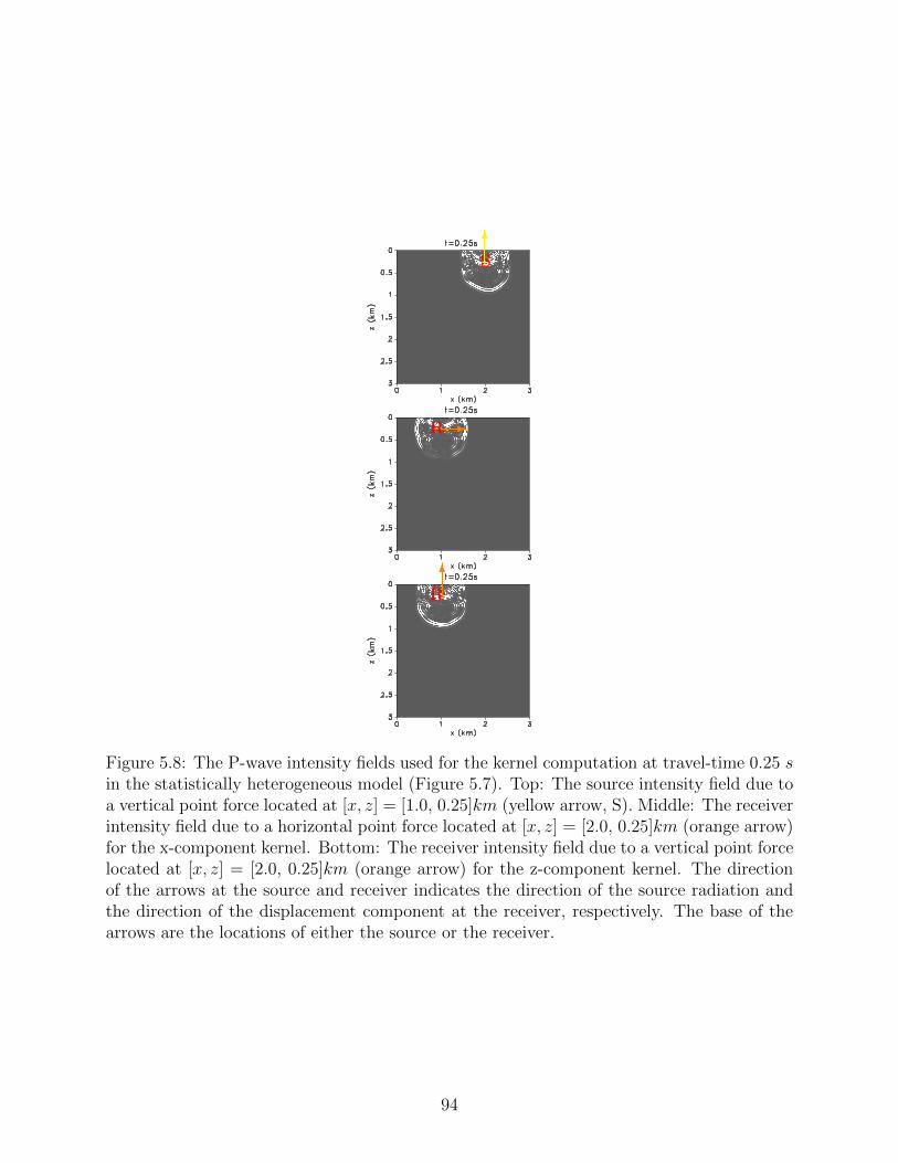
S6

-R

6R

Figure 5.8: The P-wave intensity fields used for the kernel computation at travel-time 0.25 sin the statistically heterogeneous model (Figure 5.7). Top: The source intensity field due toa vertical point force located at [x, z] = [1.0, 0.25]km (yellow arrow, S). Middle: The receiverintensity field due to a horizontal point force located at [x, z] = [2.0, 0.25]km (orange arrow)for the x-component kernel. Bottom: The receiver intensity field due to a vertical point forcelocated at [x, z] = [2.0, 0.25]km (orange arrow) for the z-component kernel. The directionof the arrows at the source and receiver indicates the direction of the source radiation andthe direction of the displacement component at the receiver, respectively. The base of thearrows are the locations of either the source or the receiver.

94

5.6.1 Sensitivity to perturbations in P-wave velocity

We compute the sensitivity kernels for a source-receiver pair embedded within the strongly

heterogeneous top layer (Figure 5.7). The source is a vertical point force located at [x, z]

= [1.0, 0.25]km (yellow arrow, Figure 5.7). Figure 5.8 shows the intensity field generated

by the point force and the receiver intensity fields with horizontal and vertical point forces

for the computation of the x- and z-components of the kernels, respectively. The intensity

fields are composed of scattered intensities from the free-surface and the reflector, a multiply

scattered intensity field, and a scattered intensity due to surface waves propagating along

the top layer. Due to the lower velocity, strong heterogeneity, free surface, and an embedded

source within the top layer, most of the scattered intensity is trapped within the top layer.

In the bottom layer, we have mostly coherently scattered waves propagating across the

layer. The forward propagating front is distorted due to the relatively broad velocity vari-

ations in the bottom layer. Figure 5.9 shows the P-wave sensitivity kernels for the x- and

z-components of the displacement fields at travel-times 0.425 s, 0.50 s, 0.75 s, and 1.00 s.

The travel-time of the first arrival is approximately 0.4 s. At the top panels of Figure 5.9

for both kernel components, the sensitivity is dominated mostly by forwardly propagating

scattered waves. The source radiation and components of the displacement fields define the

radiation of the kernel fronts shown in the top two figure panels of the kernel (Figure 5.9; t

= 0.425s and 0.5s). However for longer coda lapse times, the kernel is chaotic within the top

layer. In the two lower figure panels of Figure 5.9, the sensitivity is larger in the top layer

than in the bottom layer. Also, the kernel sensitivity within the top layer is randomized and

the kernel front is weak. The randomized nature of the kernel in the top layer results from

multiple scattering because of the strong heterogeneity within the top layer. The propagat-

ing kernel front in the bottom layer is still present but with smaller magnitude compared

with the kernel in the top layer.

95

R S6

- R S66

R S6

- R S66

R S6

- R S66

R S6

- R S66

Figure 5.9: P-wave sensitivity kernel Ki

p

of the scattered waves generated by a verticallyaligned point force source for the i= x component (left) and the i= z component (right). Thesource (yellow arrow, S) is located at [x, z] = [1.0, 0.25]km and the receiver (orange arrow,R) at [x, z] = [2.0, 0.25]km.The direction of the arrows at the source and receiver indicatesthe direction of the source radiation and the direction of the displacement component at thereceiver, respectively. The base of the arrows are the locations of either the source or thereceiver.

96

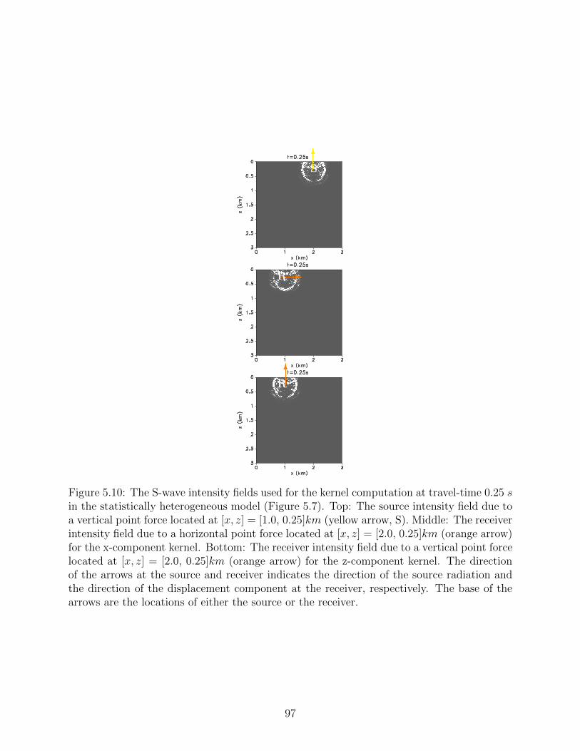
S6

-R

6R

Figure 5.10: The S-wave intensity fields used for the kernel computation at travel-time 0.25 sin the statistically heterogeneous model (Figure 5.7). Top: The source intensity field due toa vertical point force located at [x, z] = [1.0, 0.25]km (yellow arrow, S). Middle: The receiverintensity field due to a horizontal point force located at [x, z] = [2.0, 0.25]km (orange arrow)for the x-component kernel. Bottom: The receiver intensity field due to a vertical point forcelocated at [x, z] = [2.0, 0.25]km (orange arrow) for the z-component kernel. The directionof the arrows at the source and receiver indicates the direction of the source radiation andthe direction of the displacement component at the receiver, respectively. The base of thearrows are the locations of either the source or the receiver.

97

R S6

- R S66

R S6

- R S66

R S6

- R S66

Figure 5.11: S-wave sensitivity kernel Ki

s

of the scattered waves generated by a verticallyaligned point force source for the i= x component (left) and the i= z component (right). Thesource (yellow arrow, S) is located at [x, z] = [1.0, 0.25]km and the receiver (orange arrow,R) at [x, z] = [2.0, 0.25]km. The direction of the arrows at the source and receiver indicatesthe direction of the source radiation and the direction of the displacement component at thereceiver, respectively. The base of the arrows are the locations of either the source or thereceiver.

98

5.6.2 Sensitivity to perturbations in S-wave velocity

The computation of S-wave kernels uses the scattered S-wave intensities from both the

source and the receiver locations. Figure 5.10 shows the source S-wave intensity field due to

a vertical point force located at [x, z] = [1,0.25] km (yellow arrow, S) and the receiver S-wave

intensity fields for the x and z-components of the S-wave kernels. We compute the S-wave

intensity using the decomposed S-wave displacement field (equation 5.8). The receiver S-

wave displacement fields are generated by the point forces, aligned to the x and z-directions

for the x and z-components of the kernel, respectively, and located at [x, z] = [2,0.25] km

(orange arrows; Figure 5.10, middle and bottom panel). These intensity fields contain both

the intensity of the surface waves propagating within the top layer, reflected intensities both

from the free-surface and the reflector, and transmitted intensity propagating through the

bottom layer. At travel-time 0.25s, Figure 5.10 shows the nodal lines of the intensities

present in the forward propagating and reflected intensities.

Figure 5.11 shows the x- and z-components of the S-wave sensitivity kernel for travel-

times 0.50 s, 0.75 s, and 1.00 s. At travel-time 0.50 s, the x-component of the sensitivity

kernel is relatively higher at the source location (yellow arrow) compared to the receiver

location (orange arrow, S) because the amplitude is largest along the x-direction for the

source intensity field (Figure 5.10, middle panel). In the z-component of the kernel, the

sensitivities at the source and receiver locations have comparable magnitude with little in-

dication of the kernel split along the x-direction because the scattering occurs close to the

source and receiver locations. In the two bottom panels of Figure 5.11 (travel-times 0.75 s

and 1.00 s), the sensitivity within the top layer is mostly randomized but is still bounded

by a suppressed kernel front. The sensitivity within the bottom layer has relatively smaller

magnitude compared to the top layer.

The reduced sensitivities within the bottom layer (using the source-receiver pair em-

bedded within the strongly heterogeneous top layer) imply that there is weaker scattering

contributions to the scattered waves from the bottom layer across the coda lapse time. This

99

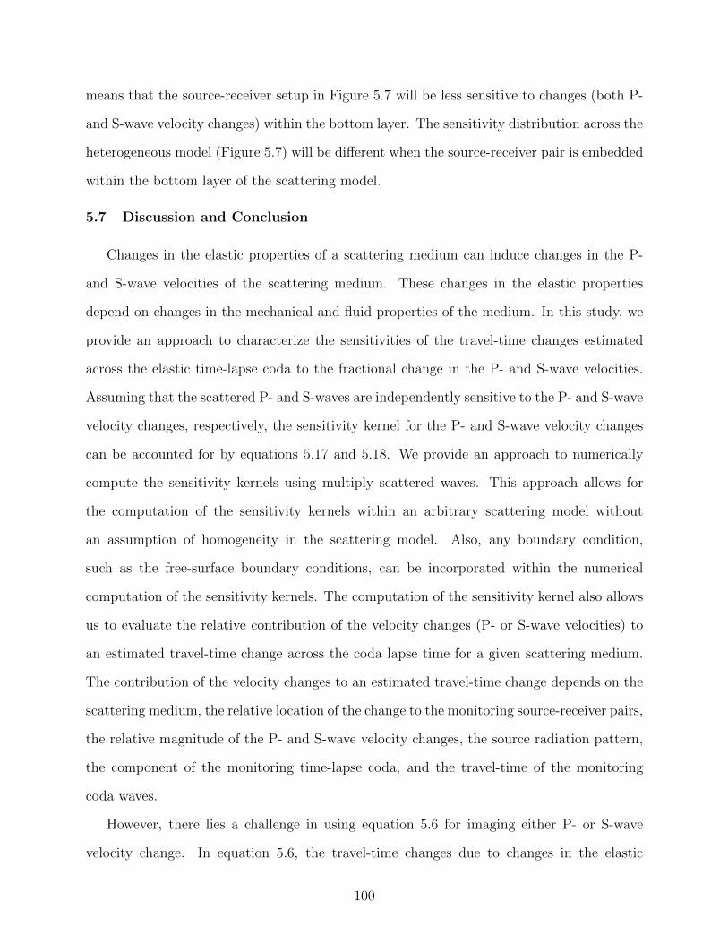
means that the source-receiver setup in Figure 5.7 will be less sensitive to changes (both P-

and S-wave velocity changes) within the bottom layer. The sensitivity distribution across the

heterogeneous model (Figure 5.7) will be di↵erent when the source-receiver pair is embedded

within the bottom layer of the scattering model.


Changes in the elastic properties of a scattering medium can induce changes in the P-

and S-wave velocities of the scattering medium. These changes in the elastic properties

depend on changes in the mechanical and fluid properties of the medium. In this study, we

provide an approach to characterize the sensitivities of the travel-time changes estimated

across the elastic time-lapse coda to the fractional change in the P- and S-wave velocities.

Assuming that the scattered P- and S-waves are independently sensitive to the P- and S-wave

velocity changes, respectively, the sensitivity kernel for the P- and S-wave velocity changes

can be accounted for by equations 5.17 and 5.18. We provide an approach to numerically

compute the sensitivity kernels using multiply scattered waves. This approach allows for

the computation of the sensitivity kernels within an arbitrary scattering model without

an assumption of homogeneity in the scattering model. Also, any boundary condition,

such as the free-surface boundary conditions, can be incorporated within the numerical

computation of the sensitivity kernels. The computation of the sensitivity kernel also allows

us to evaluate the relative contribution of the velocity changes (P- or S-wave velocities) to

an estimated travel-time change across the coda lapse time for a given scattering medium.

The contribution of the velocity changes to an estimated travel-time change depends on the

scattering medium, the relative location of the change to the monitoring source-receiver pairs,

the relative magnitude of the P- and S-wave velocity changes, the source radiation pattern,

the component of the monitoring time-lapse coda, and the travel-time of the monitoring

coda waves.

However, there lies a challenge in using equation 5.6 for imaging either P- or S-wave

velocity change. In equation 5.6, the travel-time changes due to changes in the elastic

100

velocities are coupled. Equation 5.6 can be expressed in the matrix form

⌧ = ⌧p

+ ⌧s

=⇥K

p

dx Ks

dx⇤⇥" ˆ

�s

p

s

p

�s

s

s

s

#, (5.19)

where ⌧ is an M⇥1 vector of the travel-time changes and ˆ�s

p,s

s

p,s

is a N⇥1 vector of the dis-

cretized slowness model of either the P- or S-wave. The discretized kernels Kp

dx and Ks

dx

are an M⇥N matrix of the P- and S-wave sensitivity kernel, respectively, where M is the

dimension of the estimated travel-time change and N is the dimension of the discretized

monitored medium.

The travel-time changes estimated from the time-lapse coda of a particular component

contain the contributions from both the P- and S-wave velocity changes. The coupled travel-

time changes will provide trade-o↵s for the inverted fractional changes in the P- and S-wave

velocities. The trade-o↵ can be limited by using estimates of the travel-time change from

travel-times at which the relative magnitude of one of the sensitivity kernels (P or S) is

significantly larger than the other. At travel-times close to the direct P-wave arrival time,

the P-wave sensitivity is expected to be greater than the S-wave sensitivity; conversely at

travel-times close to the direct S-wave arrival time, the S-wave sensitivity is greater. Also at

travel-times t >> r/c, where r is the source-receiver distance and c average velocity, the coda

is expected to be dominated by the S-waves [1, 97, 109] due to equipartioning of the scattered

waves. At these travel-times one expects greater contribution of the S-velocity change to

the travel-time change. Comparison of the contributions of the kernels to the travel-time

changes across the elastic coda may provide a constraint on the relative magnitude of the

fractional velocity changes in either the P- or S- wave velocity.

5.8 Acknowledgments


Methods for Complex Structures. The reproducible numerical examples in this paper use

the Madagascar open-source software package freely available from http://www.ahay.org.

101

CHAPTER 6

TIME-LAPSE IMAGING OF LOCALIZED WEAK CHANGES WITH MULTIPLY

SCATTERED WAVES: NUMERICAL EXPERIMENT


To be submitted to Journal Geophysical Research (2015)

6.1 Abstract

Multiply scattered seismic waves, due to their long path length within a finite volume,

provide information that can be used to detect and image weak time-lapse changes within a

medium. Such weak changes are usually not resolved with singly scattered waves. Previous

use of multiply scattered waves for time-lapse monitoring assume some level of statistical

homogeneity about the scattering medium. This homogeneity is usually characterized either

by a constant mean free path or di↵usion coe�cient. In a realistic medium, however, this

assumption of homogeneity likely breaks down. We demonstrate the capability of resolving

a localized time-lapse velocity change within a 3-layer scattering model using multiply scat-

tered waves. The layers within the model have di↵erent scattering properties. We localize

the weak velocity change but the resolution of the imaged change degrades with increasing

coda travel-time.

6.2 Introduction

Various monitoring tools have been developed to monitor and characterize weak changes

within a wide spectrum of media which includes the earth’s subsurface, mechanical struc-

tures such as buildings, and medical specimens. These monitoring tools range from single-

scattering wave methods (such as sonic/seismic tomography [48, 66], reflection/transmission

methods [21], and time-lapse microscopy [43]) to multiply-scattering wave methods (such

as di↵usion (acoustic) wave spectroscopy (D(A)WS) [20, 74] and coda wave interferometry

102

(CWI) [96, 97]). The strengths and limitations of these monitoring tools depend on both

the sensitivity of the monitoring data to the change in the medium and how accessible the

imaging data is for the monitoring process. It has been demonstrated that multiply scat-

tered waves are more likely to identify weak temporal changes than do single-scattered waves

[31, 44]. Multiply scattered waves, due to increased scattering, provide information about

the monitored medium that can be used to increase the resolution of the imaged medium

(for example, using reflected multiples) [8], increase illumination especially within poorly il-

luminated subsurface [28], and increase the detection of weak time-lapse changes within the

medium [76]. Increased scattering of seismic waves potentially improves the detectability of

the weak changes especially in cases where these weak changes are not resolvable with singly

scattered waves. However, because of the averaging e↵ect of multiply scattered waves and

the complexity in the travel paths of the multiply scattered waves, the spatial resolution of

the weak changes is usually not high.

Initial e↵orts in using multiply scattered waves for time-lapse monitoring were success-

fully used for detecting changes within a monitored medium [64, 76, 97, 111]. Techniques like

D(A)WS and CWI are geared toward measuring global change within a medium thereby av-

eraging the changes present across the monitored medium regardless of whether the changes

are localized or not. However, imaging the locations of weak time-lapse changes was a focus

of recent research. The first known recipe for inverting a localized change using multiply

scattered waves is given by Pacheco and Snieder [70] who relate the mean travel-time changes

to a localized slowness change. Rossetto et al. [82] introduce a technique, called LOCADIFF,

which uses the decorrelation of the time-lapse scattered waves to image a localized change

in the scattering medium. These e↵orts at localizing changes within a scattering medium

assume statistically homogeneous scattering models. How well these methods resolve weak

changes in complexly heterogeneous media especially in media where the scattered waves

have non-di↵usive behavior is yet unknown.

103

In this study, we investigate the capability of imaging a localized weak velocity change

within a scattering medium with heterogeneous statistical properties. Using a numerical

example of structurally heterogeneous model, we demonstrate the use of travel-time changes

to image a localized time-lapse velocity change within a scattering medium. In section 6.5,

we describe how the resolution of the imaged change in the model depends on the spatial

broadening of the sensitivity kernel and on the averaging out of the estimated fractional

velocity change.

6.3 Theory

Pacheco and Snieder [70] developed a sensitivity kernel K(s,xo

, r, t) that is based on

the intensity of multiply scattered waves which relates mean travel-time changes h⌧(t)i to a

localized relative velocity change �v/v(xo

) at xo

:

h⌧(t)i = �Z

V

K(s,xo

, r, t)�v

v(x

o

) dV (xo

), (6.1)

where V is the scattering volume, and s and r are the source and the receiver locations,

respectively. We estimate the travel-time changes (h⌧(t)i = -✏t) using the stretching method

[33] for a given time window of the scattered waves, where ✏ is the stretching factor. The

stretching factor is equal to the estimated fractional velocity change within the time window.

To obtain the optimal stretch factor, we minimize

min f(✏) = ||u(t+ ✏t)� u(t)||t,tw2 , (6.2)

where u(t) and u(t) are the original and the time-lapse coda signals, respectively.

Perturbation of a scattering medium can result in changes in the scattering cross-section

of the medium without a change in the velocity of the medium. Rossetto et al. [82] relate

the decorrelation D(s, r, t) between time-lapse multiply scattered waves to the time-lapse

change in the total scattering cross-subsection ��(xo

) of a medium:

D(s,xo

, r, t) =v(x

o

)��(xo

)

2K(s,x

o

, r, t). (6.3)

104

The change in the total scattering cross-subsection describes changes in the scattering prop-

erties the medium. The time-windowed decorrelation is defined as

D(s, r, t) = 1� C(s, r, t)

= 1�R

t+t

w

t�t

w

u(s, r, t0)u(s, r, t0 + ts

) dt0

[R

t+t

w

t�t

w

u(s, r, t0)2]1/2[R

t+t

w

t�t

w

u(s, r, t0)2]1/2, (6.4)

where t is the travel-time and tw

is the half-length of the time-window use to compute the

cross-correlation C(s, r, t).

Equations 6.1 and 6.3 contain the same sensitivity kernelK(s,xo

, r, t) [75], which depends

on the source and receiver locations, the scattering property of the medium, and the travel-

time of the scattered waves. The sensitivity kernel is given by

K(s,xo

, r, t) =

Rt

0 P (s,xo

, t0)P (xo

, r, t� t0) dt0

P (s, r, t), (6.5)

where P is the normalized intensity of the scattered waves [70]. The normalized intensity

Figure 6.1: Sensitivity kernel K(s,xo

, r, t) for the source-receiver pair (S-R) within a statis-tical homogeneous scattering velocity model.

or the corresponding sensitivity kernel can be computed either by using analytical intensity

models such as the di↵usion intensity model or the radiative transfer intensity model [69];

or by using a numerical approach where the sensitivity kernel is computed by convolving

numerically generated source and receiver intensity fields [38]. The intensity fields are com-

105

puted from numerically simulated scattered wavefields excited at the source and the receiver

locations. Using the numerically generated scattered intensity fields in equation 6.5, the

sensitivity kernel K(s,xo

, r, t) is obtained for every given coda lapse time t. Figure 6.1 shows

a sensitivity kernel for the source-receiver pair (S-R) using a statistical homogeneous scat-

tering velocity model. This sensitivity kernel corresponds to the scattered waves recorded

at travel-time t ' t⇤, where t⇤ is the mean free time. Given an estimate of the statistical

properties of the scattering model, the numerical solution of the wavefield gives the kernel

for imaging the time-lapse changes present in a medium, especially in a heterogeneously

complex medium.

6.4 Model setup:

To explore the capability of resolving a localized velocity change using either the es-

timated travel-time change or the decorrelation of the time-lapse data, we consider the

geometry shown in Figure 6.2, which shows both the velocity (scattering) model and the

time-lapse velocity change for our imaging problem. The velocity model is a 3 layer model,

with each layer having scattering properties of di↵erent statistical characteristics. The sta-

tistical characteristics of the top and the bottom scattering layers are structurally isotropic,

while the middle layer is statistically heterogeneous characterizing a highly fractured reser-

voir. The time-lapse change is a 0.5% velocity change in the rectangle embedded within the

middle layer shown in Figure 6.2 (bottom). To monitor and resolve this localized change, we

use two vertical receiver arrays representing two boreholes located on opposite sides of the

localized change. These boreholes record scattered waves generated by the 9 sources that

are located along a horizontal line. This source-receiver setup depicts time-lapse monitor-

ing with repeating microseismic events whose scattered waves (codas) are recorded in the 2

boreholes. We assume acoustic waves generated by an explosive source, hence we are not

accounting for the e↵ect of the source radiation and elastic seismic wave modes.

106

Figure 6.2: Numerical model for time-lapse inversion of localized velocity change with theused sources (red circles) and receivers (blue circles). Top: the reference velocity (scattering)model with the source-receiver setup and Bottom: the true localized velocity change withthe source-receiver setup.

107

6.5 Model and Data resolution

The challenge of imaging localized velocity changes or other model properties with the

multiply scattered waves lies in the resolution of the imaged model parameters. For our

imaging of the time-lapse changes, the resolution of the imaged localized changes depends

on the travel-time of the scattered waves. With increasing travel-time, the imaging data (the

travel-time changes or the decorreration) spreads out in space and the sensitivity kernel for

the time-lapse changes broadens spatially. To consider the resolution of the inverse prob-

lem, we consider both the model resolution and the data resolution. The model resolution

considers the impact of the spatial broadening of the kernel on the resolution of the inverse

solution while the data resolution evaluates the e↵ect of the data averaging. Data averaging

within the time-lapse coda wave occurs because at increasing coda lapse time, the recorded

coda results from the interference of scattered waves travelling across broader region of the

scattering medium in the presence of localized change. Figure 6.3 shows an azimuthal depen-

dence of estimated velocity changes due to a Gaussian positive velocity change (Figure 6.4,

yellow arrow points to the location of the velocity change) within a statistical homogeneous

scattering model (Figure 6.4) using the circular receiver array and a source embedded in the

middle of the model (Figure 6.4, blue dot). The azimuth of the Gaussian velocity change is

along azimuth 900 (Figure 6.3, red line) and the maximum velocity change is 1%. We show

the estimated velocity change for 36 source-receiver pairs at di↵erent azimuths for 5 coda

lapse times. Figure 6.3 shows non-zero estimated velocity changes for source-receiver pairs

with azimuth close to the azimuth of the Gaussian velocity change early in the coda (t < t⇤).

But later in the coda time (t > t⇤), the velocity change spreads to other source-receiver pairs

far from the Gaussian velocity change. The estimated velocity change becomes isotropic at

large coda lapse time (t >> t⇤). The estimated velocity changes are path-averaged velocity

changes of all the interfering scattered waves recorded within the coda wave time-window use

to estimate the velocity changes. Given that the velocity change is localized, the estimated

velocity change is a fraction of the true maximum velocity change in the medium.

108

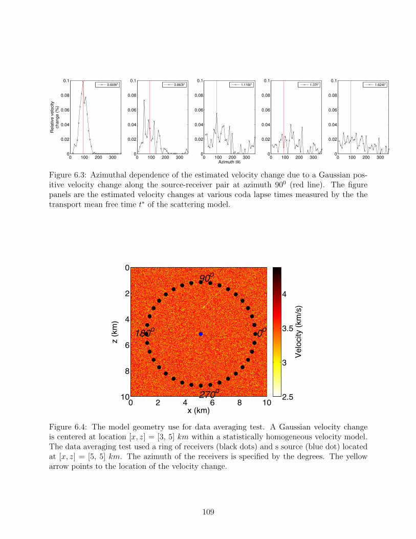
0 100 200 3000

0.02

0.04

0.06

0.08

0.1

Rela

tive v

elo

city

change (

%)

0.609t*

0 100 200 3000

0.02

0.04

0.06

0.08

0.1

0.863t*

0 100 200 3000

0.02

0.04

0.06

0.08

0.1

Azimuth (θ)

1.116t*

0 100 200 3000

0.02

0.04

0.06

0.08

0.1

1.37t*

0 100 200 3000

0.02

0.04

0.06

0.08

0.1

1.624t*

Figure 6.3: Azimuthal dependence of the estimated velocity change due to a Gaussian pos-itive velocity change along the source-receiver pair at azimuth 900 (red line). The figurepanels are the estimated velocity changes at various coda lapse times measured by the thetransport mean free time t⇤ of the scattering model.

x (km)

z (k

m)

0o

90o

180o

270o0 2 4 6 8 10

0

2

4

6

8

10

Velo

city

(km

/s)

2.5

3

3.5

4��

��

Figure 6.4: The model geometry use for data averaging test. A Gaussian velocity changeis centered at location [x, z] = [3, 5] km within a statistically homogeneous velocity model.The data averaging test used a ring of receivers (black dots) and s source (blue dot) locatedat [x, z] = [5, 5] km. The azimuth of the receivers is specified by the degrees. The yellowarrow points to the location of the velocity change.

109

Lets consider an inverse problem d = Km (ignoring noise due either to data measurement

or the model discretization), where m is the model, d is the data, and the K is a discretized

version of the Frechet derivative which describes the sensitivity of the data to the model.

We minimize the regularized least-squares objective function �:

� = ||Wd

(d�Km)||22 + �||m||22 (6.6)

where � is the trade-o↵ parameter and Wd

is the data weighting matrix whose diagonal

elements are the standard deviation of d. We determine the trade-o↵ parameter using

generalized cross-validation (GCV) [7].

The estimated model is

m = [KTWT

d

Wd

K+ �I]�1KTWT

d

Wd

Km (6.7)

where m is the actual model and I is an identity matrix. Equation 6.7 can be rewritten as:

m = Rm

m (6.8)

where Rm

= [KTWT

d

Wd

K+ �I]�1KTWT

d

Wd

K is the model resolution matrix. The model

resolution matrix Rm

explains how the inverse solution is a smeared out version of the actual

model m. From equation 6.8,

m = Rm

m =NX

i=1

mi

pi (6.9)

where N is the dimension of the model and pi are the column vectors of the model resolution

matrix Rm

. The pi vectors which are usually called the point spread functions, explain how

the ith element of the actual model is mapped to the estimated model. Following Oldenborger

and Routh [68], we can determine how well an ith parameter of the model is resolved by

solving

[KTWT

d

Wd

K+ �I]pi = KTWT

d

Wd

K�i

(6.10)

for pi using a delta function vector �i

which has 1 at the ith vector element and zeros

elsewhere. To solve for pi, we use a linear conjugate gradient algorithm. Each of the pi are

110

Figure 6.5: The coda time windows use for resolution analysis for the time-lapse imaging.Top: The used time windows for Category 1 resolution analysis and Bottom: The used timewindows for Category 2 resolution analysis.

obtained after 5 iterations. We compare the model resolution at various time windows of the

multiply scattered waves (coda). To estimate the travel-time changes across the coda, we

use 0.6 s time windows with each window overlapping 0.1 s with the previous time window.

Each time window contains about 10 cycles of the signal and the windowed signals are

tapered with a Tukey time window. Using a time window which is 10 times the dominant

period helps stabilize the estimated travel-time changes [97]. To get more data points for the

inversion, we interpolate estimated travel-time changes from time-interval 0.5 s to 0.02 s.

To evaluate the model resolution across the coda, we consider two time-window categories.

These window categories define time-windows that contain sub-time-windows. Category 1

uses a 0.55 s time window with progressive shifts of the centertime of the window to later

coda times by 0.5 s (Figure 6.5 Top). For Category 2, each of the time-windows start from

0.30 s before the first arrival. The first time window (Figure 6.5 black rectangle) extends to

0.25 s after the first arrival. The extent of the rest of the time windows increases by 0.25 s

(Figure 6.5 Bottom), i.e extending to 0.80 s, 1.05 s, 1.30 s, and 1.55 s, respectively after the

111

travel-time of the first arrival.

I

x (km)

z (k

m)

0 5 10

0

5

10

II

x (km)0 5 10

0

5

10

III

x (km)0 5 10

0

5

10

IV

x (km)0 5 10

0

5

10

V

x (km)0 5 10

0

5

10

−0.005

0.00

0.005

0.010

0.015

0.020

I

x (km)

z (k

m)

0 5 10

0

5

10

II

x (km)0 5 10

0

5

10

III

x (km)0 5 10

0

5

10

IV

x (km)0 5 10

0

5

10

V

x (km)0 5 10

0

5

10

−0.005

0.00

0.005

0.010

0.015

0.020

Figure 6.6: The point spread function pi for the inverted model at [x, z] = [5, 3] km using theTop: Category 1 and Bottom: Category 2 time-windows. The point spread function pi usestime-windows: I (black window), II (red window), III (blue window), IV (green window),and V (yellow window) in Figure 6.5.

Figure 6.6 (Top) shows the pi for the model elements located at [x, z] = [5, 3] km for

the coda time-windows in Figure 6.5 (Top). This model element corresponds to the model

location inside the middle horizon which is between z of 2.5-3.5 km (Figure 6.2). The resolved

point spread functions suggest a decrease of the model resolution with increased centertime of

the time-window (Figure 6.6). This reduced resolution results from the spatial broadening

of the sensitivity kernel. However, using the coda time-windows in Figure 6.5 (Bottom),

the velocity change pi is better resolved with increasing centertime of the time-window

(Figure 6.6 Bottom). Extending the time-windows to longer coda lapse time in Category 2

(Figure 6.5 (Bottom)), we incorporate additional model information into the inverse process

which helps to improve model resolution (Figure 6.6 Bottom). But the spatial control on

the resolved local change in the model lies on the earlier part of the coda.

112

I

sources

receiv

ers

2 4 6 8

5

10

15

20

II

sources

2 4 6 8

5

10

15

20

III

sources

2 4 6 8

5

10

15

20

IV

sources

2 4 6 8

5

10

15

20

V

sources

2 4 6 8

5

10

15

20

0.000

0.001

0.002

0.003

0.000

0.001

0.002

I

sources

rece

ivers

2 4 6 8

5

10

15

20

II

sources

2 4 6 8

5

10

15

20

III

sources

2 4 6 8

5

10

15

20

IV

sources

2 4 6 8

5

10

15

20

V

sources

2 4 6 8

5

10

15

20

0.000

0.0005

0.0010

0.0015

0.0020

Figure 6.7: Data spread function for the inverted model using the Top: Category 1 time-windows and Bottom: Category 2 time-windows. Each value is an estimated fractionalvelocity change for a given source-receiver pair.

113

Due to multiple scattering of the waves within the scattering model, there is an averaging

of the estimated travel-time change across the coda with increasing travel-time. Figure 6.7

shows the average estimated fractional velocity change across the time windows for Categories

1 and 2, as defined in Figure 6.5. These values are the average values of the subwindows

in the time windows shown in the categories. The receiver and the source numbering in

Figure 6.7 are shown in Figure 6.2. In Figure 6.7 (Top), the average estimated velocity

changes are smeared across the source-receiver pairs with increasing the centertime of the

coda waves. The smearing of the estimated velocity changes means that there are smaller

or insignificant di↵erences between the estimated velocity changes for source-receiver lines

across the location of the change and the estimated velocity changes for source-receiver lines

away from the location of the change (Figure 6.7, Top). Also due to the averaging of the

estimated velocity changes due to multiple scattering, the estimated velocity change is a

fraction of the true maximum velocity change in the medium (explained in Figure 6.3).

In Category 2, the smearing of the estimated velocity change is relatively smaller than in

Category 1. In Category 2, the average velocity change for all the time windows contains

the estimates of the velocity change near the direct or forward scattered waves.

6.6 Time-lapse inversion

To localize the weak velocity change, we minimize the objective function � (equation 6.6).

The objective function � corresponds to solving the following weighted least squares problem:

KTWT

d

d = [KTWT

d

Wd

KS�1 + �I]Sm = [KTWT

d

Wd

KS�1 + �I]mS

, (6.11)

where d is the estimated travel-time change �t, and m = S�1mS

is the fractional velocity

change. The sensitivity weighting matrix S is a diagonal matrix with the elements Sij

=

�ij

wj

, where the weights wj

are given by [46]:

wj

=

NX

k=1

K2kj

!1/2

, j = 1, ...,M ; (6.12)

114

where N is the number of data and M is the number of the discretized model space. We

apply S to suppress the elevated sensitivity at the source and receiver locations [38]. The

sensitivity weighting matrix acts as a preconditioner for the inversion problem. To solve

equation 6.11, we use a linear conjugate-gradient method. All the imaged velocity changes

in this subsection are obtained after 5 iterations.

The inverted velocity images correctly recovers the location of the velocity change, albeit

with some artifacts. For the time windows shown in the top panel of Figure 6.8, the resolution

of the inverted velocity change varies with di↵erent coda time windows. Figure 6.8B provides

the best resolved and localized image of the velocity change. In Figure 6.8A, there are smears

in the inferred velocity change towards the receivers above the velocity change. These smears

are caused by the forward scattered waves that have their highest sensitivity along the source-

receiver lines that cut across the location of the velocity change. At later times (Figure 6.8B,

C, and D), there is an additional artifact which is centered at location [x, z] = [5, 5.8]

km. This artifact is induced by the intersection of kernel fronts which have relatively large

amplitudes compared to the inner part of the sensitivity kernel. In Figure 6.8D the artifact

is weaker due to the weakening of the kernel front with traveltime.

6.7 Conclusions

In this study, we demonstrate the capability of resolving localized weak changes within

heterogeneous scattering media using multiply scattered waves. Our imaging algorithms

build on the work of Pacheco and Snieder [70] and Rossetto et al. [82]. Using estimated time-

lapse travel-time change, we demonstrate with a numerical example how well we can localize

a weak velocity change within a heterogeneous 3-layer scattering model. We image this

localized velocity change in the 3-layer model without assuming any statistical homogeneity

of the scattering model. For this model, our imaging recipe resolves well the location of the

velocity change especially early in the coda wave. However, the resolution of the imaged

velocity change progressively decreases with increasing travel-time of the coda waves we use

in the imaging. The decrease in the resolution of the velocity change results from the spatial

115

x (km)

z (k

m)

A

0 5 10

0

2

4

6

8

10 −0.1

0

0.1

0.2

0.3

0.4

x (km)

z (k

m)

B

0 5 10

0

2

4

6

8

10 −0.1

0

0.1

0.2

0.3

0.4

x (km)

z (k

m)

C

0 5 10

0

2

4

6

8

10 −0.1

0

0.1

0.2

0.3

0.4

x (km)

z (k

m)

D

0 5 10

0

2

4

6

8

10 −0.1

0

0.1

0.2

0.3

0.4

Figure 6.8: Inverted fractional velocity change using various coda time windows. Top inset:a typical recorded coda signal with time windows use to invert the velocity changes. Invertedvelocity change in A: with black time window, B: with red time window, C: with blue timewindow, and D. with green time window. The black box shows the extent of the velocitychange.

116

broadening of the sensitivity kernel with travel-time and the averaging out of the estimated

changes across the sources and receivers.

6.8 Acknowledgments


Methods for Complex Structures. The reproducible numeric examples in this paper use the

Madagascar open-source software package freely available from http://www.ahay.org.

117

CHAPTER 7

TIME-LAPSE IMAGING OF LOCALIZED WEAK CHANGES WITH MULTIPLY

SCATTERED WAVES: LABORATORY EXPERIMENT

Chinaemerem Kanu1 2, Roel Snieder1 2, Ernst Niederleithinger1 2, and Sven Grothe2

To be submitted to Ultrasonics (2015)

7.1 Abstract

Mechanical structures can undergo changes due to wear and tear due to natural or man-

made processes. These processes usually induce stress or temperature changes in the struc-

tures which create either irreversible or partially reversible changes on the rigidity of the

structures. We demonstrate the use of multiply scattered ultrasound waves in monitoring

and imaging localized changes within concrete blocks. We present a laboratory experiment

with two concrete blocks where in one we apply a localized stress change and in the other

a temperature change from a localized heating cartridge. Using the intensity of multiply

scattered waves, we imaged the changes induced by both the stress and temperature changes

within the concrete blocks. We accurately localize the change within the concrete blocks

using the decorrelation of the time-lapse coda and the fractional velocity changes.

7.2 Introduction

Mechanical structures, such as buildings, roads, and bridges, are known to undergo wear

and tear over time which can compromise the longevity of these structures. The resulting

defects within the structures can be weak and hard to detect, so that their e↵ect on the

overall integrity of the structures are felt late. For an optimal management of the mechanical

structures and the overall safety of their use, there is a need to monitor the mechanical

1Center for wave phenomena, Colorado School of Mines2BAM (Federal Institute for Materials Research and Testing), Berlin, Germany

118

structures continuously with a monitoring tool or method that has the sensitivity to identify

the defects before they escalate to a destructive stage. Coda wave interferometry (CWI)

provides a tool to identify weak changes or defects within a scattering medium, such as in

monitoring of volcanoes [56], subsurface velocity changes near faults or in the near subsurface

[76, 87], or changes in concrete blocks induced by either stress changes or temperature changes

[31, 100]. The higher sensitivity of the coda waves to weak changes compared to the singly

scattered waves allows for the detection of weak changes within scattering media. However,

the coda waves provide spatially averaged estimates of the weak changes especially in cases

where the time-lapse changes are localized. This spatial averaging limits the ability to resolve

the locations of the weak changes.

We present two laboratory experiments with concrete blocks in which we monitor weak

changes. In one of the experiments we monitor a weak change due to an induced compressive

stress (force) at the opposite sides of the concrete block while in the second experiment we

monitor changes due to temperature changes within a di↵erent concrete block. The temper-

ature changes in the concrete block is either due to the ambient temperature fluctuations

within the concrete and due to a localized heating provided by a heat cartridge within the

concrete block. In this study, we apply an imaging algorithm based on the scattered intensity

of the time-lapse coda to localize the weak changes within the concrete blocks [38].

7.3 Theory

Velocity changes and changes in the scattering properties of a heterogeneous medium

induce changes within time-lapse coda waves. Pacheco and Snieder [70] and Rossetto et al.

[82] related the travel-time changes and decorrelation of the time-lapse coda waves to ve-

locity changes and perturbations in the scattering cross-section of the medium, respectively.

Using probability density functions, Pacheco and Snieder [70] give the relationship between

a localized fractional velocity change �v/v(xo

) at xo

and the estimated travel-time changes

119

h⌧(t)i induced by the velocity change:

h⌧(t)i = �Z

V

K(s,xo

, r, t)�v

v(x

o

) dV (xo

), (7.1)

whereK(s,xo

, r, t) is the sensitivity of the travel-time change to the localized velocity change

in the scattering medium. The sensitivity, which is computed using the intensity of the

scattered wavefield [38], depends on the source and receiver locations, the scattering property

of the medium, and the travel-time of the scattered waves. Similarly, Rossetto et al. [82]

relate the decorrelation D(s, r, t) between time-lapse multiply scattered waves to the time-

lapse change in the total scattering cross-subsection ��(xo

) of a medium:

D(s,xo

, r, t) =v

2

Z

V

K(s,xo

, r, t)��(xo

) dV (xo

), . (7.2)

The change in the total scattering cross-subsection describes a change in the scattering

property the medium.

The travel-time changes h⌧(t)i and the decorrelation D(s, r, t) can be estimated for a

given source-receiver pair by comparing the time-lapse coda waves. Practically, the time-

windowed decorrelation is obtained using

D(s, r, t) = 1� C(s, r, t)

= 1�R

t+t

w

t�t

w

u(s, r, t0)u(s, r, t0 + ts

) dt0

[R

t+t

w

t�t

w

u(s, r, t0)2]1/2[R

t+t

w

t�t

w

u(s, r, t0)2]1/2, (7.3)

where t is the travel-time and tw

is the half-length of the time-window use to compute

the cross-correlation C(s, r, t). We estimate the travel-time changes (h⌧(t)i = -✏t) using

the stretching method [33] for a given time window of the scattered waves, where ✏ is the

stretching factor. The stretching factor is equal to the estimated fractional velocity change

within the time window. To obtain the optimal stretch factor, we minimize

min f(✏) = ||u(t+ ✏t)� u(t)||t,tw2 , (7.4)

where u(t) and u(t) are the original and the time-lapse coda signals, respectively.

120

The sensitivity kernel is given by

K(s,xo

, r, t) =

Rt

0 P (s,xo

, t0)P (xo

, r, t� t0) dt0

P (s, r, t), (7.5)

where P is the normalized intensity of the multiply scattered waves [70]. The sensitivity

kernel K(s,xo

, r, t) can be estimated either by using the analytical [70, 82] or numerical

methods [38]. The analytical method of computing K(s,xo

, r, t) usually uses the di↵usion

[72, 92, 112] or the radiative transfer formulation of the scattered intensity [69]. However, the

analytical methods typically assumes that the scattering medium is statistical homogeneous.

In a medium where the scattering properties are spatially varying, the numerical method

of computing the sensitivity kernel is preferred [38], because the sensitivity is computed

numerically with an a prior estimate of the scattering model by numerically computing the

normalized intensity of the multiply scattered waves.

7.4 Laboratory experiment in a concrete block

Concrete block with stress changes

To demonstrate the capability of resolving weak changes within a physical scattering medium,

we invert for a change induced by a localized stress loading on the surface of a concrete block

with dimensions 1.5 x 1.5 x 0.5 m3. The concrete block, with an average P-wave velocity

of 4 km/s, consists of aggregate (which act as scatterers) of size approximately 32 mm and

reinforcements in half of the block (Figure 7.1). The reinforcement consists of a rebar mesh

of 8 mm rods spaced at 150 mm intervals. Within the block, we embedded 18 transducers

that serves both as sources and receivers. Because of coupling issues, we only use 10 of

the transducers (Figure 7.2). Table 7.1 gives the locations of the used transducers. These

10 transducers are connected to ultrasound transmitting and receiving equipment via a

multiplexer. The multiplexer connects an amplified signal generated by a function generator

to a given transducer selected at a given time (Figure 7.3). This selected transducer acts as

the source while the rest of the transducers serve as receivers. The recorded signals are sent

to an Analog-to-Digital (A/D) device and then to data storage. A given load experiment

121

results to a total of 90 traces. The source signal has a dominant frequency of 60 kHz.

Figure 7.1: Schematic of the 3D concrete block for time-lapse monitoring

Figure 7.2: Outline of the 3D concrete block with the locations of the used transducers.The transducers are embedded within the concrete block. The transducer locations are theprojection along the z-axis (left) and along the x-axis (right).

To induce a local change on the concrete block, we apply a stress loading on a 30 mm

borehole drilled through the block along the z-axis. The borehole is located at (x = 0.95 m,

y = 0.325 m). A 20 mm bolt is put through the borehole and fastened on both sides with

load distribution steel plates and nuts. The load steel plates are 0.1 x 0.1 m2 wide and 10

mm thick. On one side of the block, a calibrated load cell (a piezoelectric sensor) is placed

between the load steel plate and an additional disc. The load cell is used for current supply

122

Figure 7.3: The electrical and mechanical setup of the stress loading experiment.

and voltage measurement. This experiment which was designed and setup at the Federal

Institute for Materials Research and Testing, Berlin, Germany (known as BAM) involves

monitoring series of stress loading ranging from 0 kN to 100 kN and back to 0 kN .

Table 7.1: Transducer coordinates.

Transducer No. x (mm) y (mm) z (mm)16 1000 375 374.517 500 375 374.518 250 375 374.519 1000 1125 83.522 1000 375 83.523 500 375 83.524 250 375 83.528 1105 160 22029 605 160 22030 355 160 220Load 950 325 0 - 500

Figure 7.4 shows typical signals recorded at transducer 17 when transducer 16 acts as

a source. At t=0 each receiver records a event from the source induced electrical response.

We use this electrical event (Figure 7.4 (black ellipse)) to book-keep the onset time of the

source signals. This event is removed prior to time-lapse analysis of the signals. The rest of

the recorded scattered waves in the signals consist of ballistic and coda waves resulting from

123

wave scattering within the concrete block. The two signals in Figure 7.4 are from repeated

experiments on a given stress load displaying the strong repeatability of the signals.

Figure 7.4: Typical time-lapse coda signals recorded at transducer 17 due to a source attransducer 16 from the stress loading experiment. The black ellipse indicate the electricalsignal use to book-keep the source unset time.

Concrete block for temperature changes

Figure 7.5 shows both the pictorial and schematic views of the concrete block we use for

monitoring changes due to temperature changes. The experiment was conducted in an

outdoor field in Berlin that is owned by BAM. The concrete block has a dimension of 5

x 4 m2 and 0.8 m thick consisting of a concrete mix based on the C30/37 mix design

given in the European (Eurocode2) or German guidelines (DIN 1045-1). There is a heat

cartridge H connected via a heating pipe from outside into the concrete block to induce

local temperature changes within the block (Figure 7.5 bottom, cyan line). We monitor the

time-lapse local temperature changes using sensors that are attached at the side faces of the

concrete block. We have ten sensors at each of the four sides of the concrete block. The

sources for the monitoring ultrasonic waves are given as sensors (S1-S20) while sensors R1-

R20 are the recording sensors of the scattered (ultrasonic) waves (Figure 7.5 Bottom). The

electrical setup of the temperature experiment is similar to the setup in the stress experiment

(Figure 7.6). However, in the temperature experiment, we use an ultrasonic source signal

of a dominant frequency of 25 kHz. Figure 7.7 shows an example of the time-lapse signals

recorded by sensor R5 due to source signal from sensor S5.

124

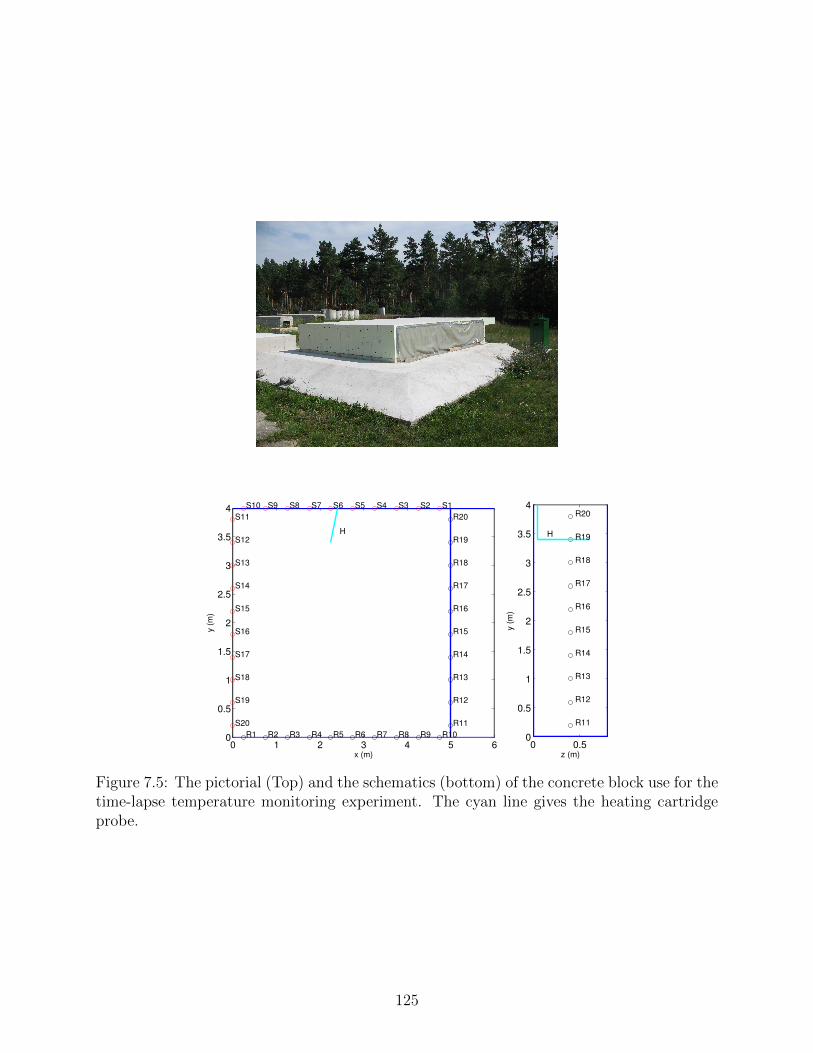
0 1 2 3 4 5 60

0.5

1

1.5

2

2.5

3

3.5

4

H

S1S2S3S4S5S6S7S8S9S10

S11

S12

S13

S14

S15

S16

S17

S18

S19

S20

R1 R2 R3 R4 R5 R6 R7 R8 R9 R10

R11

R12

R13

R14

R15

R16

R17

R18

R19

R20

x (m)

y (m

)

0 0.50

0.5

1

1.5

2

2.5

3

3.5

4

R11

R12

R13

R14

R15

R16

R17

R18

R19

R20

H

z (m)

y (m

)

Figure 7.5: The pictorial (Top) and the schematics (bottom) of the concrete block use for thetime-lapse temperature monitoring experiment. The cyan line gives the heating cartridgeprobe.

125

Trigger

Storage

PC

A

D

Receiver

MUX

MUXTransmitter

Preamplifier

(x60)Specimen

TTLWavelet

Figure 7.6: The electrical and mechanical setup of the stress loading experiment.

0 2 4 6 8 10−1

−0.5

0

0.5

1

time (ms)

am

plit

ud

e

Figure 7.7: Typical coda signal recorded by sensor R5 due to a source at sensor S1 from thetemperature experiment.

126

The fundamental solution of the heat transfer equation for an infinite 3D homogeneous

medium with a thermal conductivity k using a delta temperature forcing of maximum 10 C

is

T (x, t) =1p4⇡↵t

e

�||x�x0||2/4↵t, (7.6)

where ↵ is the thermal di↵usivity of the heated medium. The thermal di↵usivity is given

as k/⇢cp

, where ⇢ is the density of the medium and cp

is the specific heat capacity of the

medium.

��

Figure 7.8: Temperature history of the time-lapse heating experiment. The question markindicates that the temperature curve between 1:11pm (4th of April) and 8am (5th of April)is unknown.

Figure 7.8 shows the temperature history of the time-lapse temperature experiment at

the location of the heat cartridge. The time-lapse temperature change occurs between 8am at

the 4th of April, 2014 and 8am at the 5th of April, 2014. The ambient temperatures measured

were 11.370 C on the 4th and 10.410 C on the 5th of April. During the baseline measurement

on 4th of April, the temperature of the heating cartridge was set at 1000 C. However, at

11:11am on 4th of April, the heating temperature was increased to 5100 C for a period of 2

hours before the cartridge was turned o↵. The decay of the temperature after 1:11pm on the

4th of April is based on the solution of the heat transfer equation in equation 7.6. To estimate

the temperature distribution across the heated concrete block at the time-lapse time (8am

on the 5th of April), we need the initial condition of the temperature distribution across the

127

concrete, i.e., the temperature distribution across the concrete at 1:11pm on the 4th of April.

We do have point temperature measurements at the location of the heat cartridge and 0.2 m

away from the heat cartridge within the concrete. The temperature measurements at the

location of the heat cartridge and 0.2 m away from the heat cartridge are 5100C and 470C,

respectively.

Let’s assume that the temperature distribution at 1:11pm on the 4th of April (the initial

temperature condition TIC

(x, t) ) has a Gaussian characteristics defined as:

TIC

(x, t) = 510e�||x�x0||2/2�2, (7.7)

where � is the width of the temperature anomaly during the initial temperature condition

time. This assumed Gaussian characteristics ignores the e↵ect of the reflecting boundaries.

This is because we do not have the exact location of the temperature sensor 0.2 m away from

the heat cartridge. Using the temperature measurement 0.2 m away from the heat cartridge,

the estimated width of the temperature anomaly during the initial temperature condition

time � is 0.092 m. Therefore,

TIC

(x, t) = 510e�||x�x0||2/0.0168m2. (7.8)

Assuming TIC

(x, t) as the initial condition for the heat conduction, the solution of the

heat conduction within the concrete at the time-lapse time (TT

(x, t)) is

TT

(x, t) =

Z

V

T (x� x0, t)TIC

(x0, t) dx0, (7.9)

TT

(x, t) =510p4⇡↵t

e

�||x�2x0||2/(4↵t+0.0168)m2. (7.10)

The typical thermal di↵usivity of concrete medium ranges from 0.002-0.007 m2/hr [115].

Using equation 7.10 and assuming a thermal di↵usivity ↵ of 0.005 m2/hr for a concrete

material, the approximate distribution of the temperature (equation 7.10) within the concrete

material is shown in Figure 7.9. The temperature at the location of the heat cartridge is

463.840C during 8am of the 5th of April, 2014. Therefore the temperature curve in Figure 7.8

decreases to approximately 463.840C on 8am of the 5th of April.

128

x (m)

y (m

)

H


S11

S12

S13

S14

S15

S16

S17

S18

S19

S20

R1 R2 R3 R4 R5 R6 R7 R8 R9 R10

R11

R12

R13

R14

R15

R16

R17

R18

R19

R20

0 1 2 3 4 50

0.5

1

1.5

2

2.5

3

3.5

4

0

0.2

0.4

0.6

0.8

1

Figure 7.9: Normalized temperature distribution across the heated concrete medium at theend of the temperature history in Figure 7.8 using equation 7.10. The cyan line is the heatingcartridge probe.

129

7.5 Data analysis

Using coda wave interferometry analysis (CWI), we can estimate the fractional velocity

change �v/v or the decorrelation D of the time-lapse coda signals for a specific time window

using either the stretching method [33], or by computing D = 1 � Cmax

(equation 7.3),

respectively.

In the stretching method, we stretch one of the coda signal by a constant stretch factor

relative to the second time-lapse coda signal. The optimal stretch factor, which is the

estimated fractional velocity change within the windowed time-lapse coda, is determined

by the stretch factor that minimizes the L2 norm of the di↵erence between the time-lapse

coda signals. Figure 7.10 and Figure 7.11 show the estimated decorrelation D and the

estimated fractional velocity change �v/v from the 90 time-lapse coda signals in the stress

experiment, respectively. The estimates of the decorrelation or the fractional velocity change

is random and larger before the first arrival because of low signal-to-noise ratio. The figures

compare changes due to load jumps from 5 kN to 10 kN and from 5 kN to 15 kN . The

changes are larger for the 5 kN -15 kN load jump than for the 5 kN -10 kN load jump

(Figure 7.10 and Figure 7.11). The estimated changes are more pronounced for later coda

lapse times. Compare traces 28-35 with traces 38-45. Traces 38-45 generally have larger

time-lapse velocity changes and decorrelations than traces 28-35. The di↵erences in the

time-lapse changes across the traces are due to the arrangements of the sensors. Figure 7.12

provides a picture of the recorded time-lapse change for individual transducer pairs. The

figure shows an indication of a localized change. Figure 7.12 shows the average decorrelations

estimated from the time-lapse scattered waves arriving between 0.28 ms and 0.58 ms after

the first arrival. The decorrelations are estimated using the time-window in time-lapse coda

in Figure 7.12 (top). Larger decorrelation results from the load jump of 5 kN to 15 kN

compared to the load jump of 5 kN to 10 kN and also from the sensor pairs close to the

location of the compressive loads.

130

trace

time

(m

s)

decorrelation

20 40 60 80

0.2

0.4

0.6

0.8

1

1.2

1.4

1.6

0

0.1

0.2

0.3

0.4

0.5

0.6

0.7

0.8

0.9

1

trace

time

(m

s)

decorrelation

20 40 60 80

0.2

0.4

0.6

0.8

1

1.2

1.4

1.6

0

0.1

0.2

0.3

0.4

0.5

0.6

0.7

0.8

0.9

1

Figure 7.10: Record of the estimated time-lapse decorrelation due to a load jump from 5 kNto 10 kN (left) and a load jump from 5 kN to 15 kN (right). The record contains 90 traces(due to 10 pairs of sensors with no trace for the same sensor combination). The records arearranged according to the source sensor records.

trace

time

(m

s)

relative velocity change (%)

20 40 60 80

0.2

0.4

0.6

0.8

1

1.2

1.4

1.6

−0.5

−0.4

−0.3

−0.2

−0.1

0

0.1

0.2

0.3

0.4

0.5

trace

time

(m

s)

relative velocity change (%)

20 40 60 80

0.2

0.4

0.6

0.8

1

1.2

1.4

1.6

−0.5

−0.4

−0.3

−0.2

−0.1

0

0.1

0.2

0.3

0.4

0.5

Figure 7.11: Record of the estimated time-lapse relative velocity change in % due to a loadjump from 5 kN to 10 kN (left) and a load jump from 5 kN to 15 kN (right). The recordcontains 90 traces (due to 10 pairs of sensors with no trace for the same sensor combination).The records are arranged according to the source sensor records.

131

Figure 7.12: Time-lapse decorrelation due to stress loading from 5 kN to 10 kN (left) andfrom 5 kN to 15 kN (right) at X. The colored lines between two sensors are the estimatedaverage decorrelation between the time lapse signals using equation 7.3 for the time-windowin time-lapse coda (top). The decorrelations for each sensor pairs are not restricted to theconnecting colored lines.

132

Figure 7.13 shows the estimated decorrelation and velocity (negative) changes for the

time-lapse heating experiment for the source-receiver pairs using the time-window shown

with the black box in the top panel of Figure 7.13. For each source-receiver pair, the time-

window is centered at a delay time of 2.5 ms from the first arrival times. The decorrelation

and velocity (negative) changes are spread out across the source-receiver pairs but there are

larger decorrelation and velocity (negative) changes for the source-receiver pairs across the

heat cartridge (lying between S5 and S6).

01

23

45

0

1

2

3

40

0.5

R11R10

R12

R9

R13R14

R8

R15R16

R7

R17

R6

R18R19

R5

x (m)

R20

R4

S1

R3

S2

R2

S3

R1

S4

S20

S5

S19S18

S6

S17

S7

S16S15

y (m)

S8

S14S13

S9

S12S10

S11

z (m

)

−0.25

−0.2

−0.15

−0.1

−0.05

0

0.05

0.1

0.15

0.2

0.25

01

23

45

0

1

2

3

40

0.5

R11R10

R12

R9

R13R14

R8

R15R16

R7

R17

R6

R18R19

R5

x (m)

R20

R4

S1

R3

S2

R2

S3

R1

S4

S20

S5

S19S18

S6

S17

S7

S16S15

y (m)

S8

S14S13

S9

S12S10

S11

z (m

)

−0.25

−0.2

−0.15

−0.1

−0.05

0

0.05

0.1

0.15

0.2

0.25

Figure 7.13: Time-lapse fractional velocity change (%) and decorrelation due to temperaturechange within the concrete block. The colored lines between two sensors are the estimatedchanges (fractional velocity change (left) and decorrelation (left)) between the time lapsesignals for the time-window in time-lapse coda (top). The changes for each sensor pairs arenot restricted to the connecting colored lines.

7.6 Time-lapse inversion

Here, we invert for weak changes within the heterogeneous 3D concrete blocks. These

weak changes are induced either by a compressive localized stress or a localized change in

133

temperature within the concrete block. To invert for the changes induced by the stress

loadings or the localized temperature change, we solve

KTWT

d

d = [KTWT

d

Wd

K+ �I]m, (7.11)

where KT is a discretized version of the sensitivity kernel (equation 7.5) of the travel-time

change or the decorrelation to the localized change in the scattering model using multiply

scattered waves, Wd

is the data weighting matrix, � is a regularization parameter, and m

defines the inverted change in the scattering medium which are either the change in velocity

or the change in the scattering cross-section. The data is either the decorrelation of the

time-lapse coda or the travel-time change from the time-lapse coda. To solve equation 7.11,

we use linear conjugate-gradient method.

We compute the sensitivity kernel using radiative transfer model of the scattered intensity

in the block [38] with fully reflecting boundary conditions [82] on the planar boundaries of

the concrete block. We currently assume acoustic wave scattering but future inversions of

the weak change in the concrete block will incorporate elastic scattering. To estimate the

sensitivity kernel we estimate the average mean free path by fitting the intensities of the coda

waves using radiative transfer intensity which depends on the mean free path. We estimate

the mean free path to be approximately 1.52 m which corresponds to a mean free time of

0.362 ms using P-wave velocity for the stress experiment and a mean free path of 3.75 m

and a mean free time of 0.893 ms for the temperature experiment. The time window we use

for the inversion extends beyond the mean free time.

Figure 7.14 shows the inverted solution of the weak changes within the concrete block

in the stress experiment at z = 0 m for stress loading of 5-10 kN and 5-15 kN using the

time window in Figure 7.14 (top). For the stress experiment we use the decorrelation of the

time-lapse coda for the inversion. These stress loadings induce a relatively more significant

and consistent perturbation on the amplitude of the coda signals than on the phase of the

coda. Figure 7.14 shows the resolved change which is at close proximity to the point of the

stress loading for both stress experiments. The resolution of the weak change depends on

134

the source-receiver coverage and the time windows we use for the inversion due to the spatial

broadening of the sensitivity kernel with travel-time [38].

� � � �

Figure 7.14: Inverted change due to stress loading from 5 kN to 10 kN (left) and from 5kN to 15 kN (right) at X. Top inset: Time-lapse coda showing the time-window used forthe inversion.

Using the same inversion algorithm, we invert for the time-lapse change within the con-

crete block in Figure 7.5 due to a localized temperature change. Figure 7.15 shows the

inverted velocity change in percent resulting from a heating experiment at the location of

the heating cartridge. We use scattered waves recorded at the same hour of the day to

reduce the e↵ect of ambient temperature change. Figure 7.15 compares the imaged velocity

change and the imaged change in the scattered cross-section with the location of the heat-

ing cartridge. We use estimated fractional velocity change and decorrelation extracted from

time-windows centered at around 2.5ms after the first arrival (Figure 7.15 top). The figures

show that using the estimated change from the coda time-window beyond the mean free time,

we can accurately localize the location of the temperature change induced by the heating

within the concrete. The imaged velocity change suggests that temperature changes induces

135

x (m)

y (m

)

H


S11

S12

S13

S14

S15

S16

S17

S18

S19

S20

R1 R2 R3 R4 R5 R6 R7 R8 R9 R10

R11

R12

R13

R14

R15

R16

R17

R18

R19

R20

0 1 2 3 4 50

0.5

1

1.5

2

2.5

3

3.5

4

−5

0

5

x (m)

y (m

)

H


S11

S12

S13

S14

S15

S16

S17

S18

S19

S20

R1 R2 R3 R4 R5 R6 R7 R8 R9 R10

R11

R12

R13

R14

R15

R16

R17

R18

R19

R20

0 1 2 3 4 50

0.5

1

1.5

2

2.5

3

3.5

4

−0.4

−0.3

−0.2

−0.1

0

0.1

0.2

0.3

0.4

Figure 7.15: Inverted change due to localized temperature change due to a heating cartridgeat H (Figure Figure 7.5 (Bottom)) using the travel-time changes and decorrelation esti-mated at the coda time window (black rectangle) in Top inset. In the Bottom inset: (left)the inverted relative velocity change (in percentage) using estimated travel-time changes and(right) the inverted change in the scattering cross-section (in m2) using estimated decorre-lation.

136

a negative velocity change around the heating cartridge. The negative velocity change im-

plies that at 8am of 5th of April, 2014, the temperature within the concrete surrounding the

heating cartridge has not dropped down to 1000 C [31, 63]. The elevated temperature at

8am of 5th of April, 2014 is supported by the modeled time-lapse temperature distribution

within the medium in Figure 7.9.

7.7 Conclusion

This study demonstrates the use of time-lapse ultrasound waves to monitor changes

induced within heterogeneous concrete blocks by stress and heat changes. We monitor time-

lapse localized changes within a C30/37 concrete block due to an induced compressive stress

applied on opposite sides of the concrete block. In another concrete block, we monitor

changes induced by elevated localized heat within the block that is induced by an embedded

heating cartridge. To image the changes within the concrete blocks, we use imaging algo-

rithms based on the work of Pacheco and Snieder [70] and Rossetto et al. [82]. The imaging

algorithms allow for the use of either time-lapse fractional velocity changes or the decorre-

lation of the time-lapse ultrasound signals to image the change. To invert for the localized

change within the concrete blocks, we solve a regularized least squares problem using linear

conjugate gradient. We accurately localized the change within the concrete blocks using

decorrelation and fractional velocity changes estimated with coda lapse times beyond the

mean free time of the concrete blocks.

137

CHAPTER 8

TIME-LAPSE MONITORING ACROSS UTAH AND EASTERN SECTION OF BASIN

AND RANGE

Chinaemerem Kanu1, Roel Snieder1 and Kristine Pankow2

Published in Journal Geophysical Research (2014)

8.1 Abstract

The Eastern part of the Basin and Range, extending to the Wasatch fault region, is

an actively deforming region characterized by varieties of extensive features and prominent

seismicity along the inter-mountain seismic belt. The present day deformation of the inter-

mountain seismic belt and the eastern Basin and Range provinces, motivates an interest in

continuous monitoring of the region. In this study we monitor time-lapse velocity changes

within Utah and eastern Nevada using coda waves generated by repeatable explosions. This

monitoring characterizes velocity changes within the region from June to September of 2007.

We observe, both temporally and spatially, variable velocity changes within the monitored

region, with a maximum path-average velocity change of 0.2%. This suggests a significant

change in the velocity within the region given the short monitoring duration. Correlation

of the temporal variation of the average velocity change with strains derived from GPS

detrended displacements suggests that the velocity change might be driven by the broad

deformation within the monitored region.

8.2 Introduction

Coda wave interferometry is an e↵ective tool to monitor time-lapse changes within a

medium, especially if these changes are weak [97]. Coda wave interferometry allows us to

1Center for wave phenomena, Colorado School of Mines2University of Utah Seismograph Stations, Salt Lake City, Utah

138

extract subsurface changes from scattered seismic waves generated from repeated sources.

With identical sources and negligible noise, di↵erences within the seismic coda (such as time

shift and amplitude decay) provide information about the changes within the monitored

medium through which the coda wave travels. Due to the redundancy in the coda waves and

possibly increased illumination of the subsurface by the scattered waves, the sensitivity of

the scattered waves to perturbations within the subsurface usually increases with increasing

travel time. This sensitivity of the multiply scattered waves has allowed for monitoring

weak changes in velocity that are in the order of 0.1% [96]. Multiply scattered waves have

successfully been used to monitor velocity changes along fault regions [76, 87], detect in-

situ velocity changes due to stress changes in a mine [31], characterize near-surface velocity

changes [62, 89], monitor temporal changes within volcanic regions [56], and detect far-field

stress-induced velocity changes (such as those induced by solid earth tides) [100].

The monitored region in this study covers the Basin and Range physiographic province,

the transition from the Basin and Range to both the Middle Rocky Mountains and the

Colorado Plateau, and the Snake River Plain (Figure 8.1). This region is characterized by

active deformation, primary extension mostly east-west directions for the Basin and Range

and more southeast to northwest extension in the Snake River Plain [77]. In addition to the

major phyisographic provinces, the region is characterized by mostly north-south trending

normal faults, including the Wasatch fault. While there is di↵use seismicity throughout the

region, most of the seismicity is concentrated with the Intermountain Seismic Belt (ISB), a

zone of shallow seismicity that extends from Montana to Arizona [95]. Unique to western

Utah are basins composed of soft sediments related to Lake Bonneville (a late Pleistocene

pluvial lake). In the Salt Lake Basin these soft sediments are greater than 1 km deep in

some locations [83]. The soft sediments are potentially susceptible to both near-field and far-

field stress loadings. Taken together, the active regional deformation, localized seismicity

and faulting, and surface geology, provide a complex contemporary deforming area with

potentially small- and large-scale changes in both time and space.

139

Figure 8.1: USArray transportable array given by the red squares. The location of theexplosion (source) is given by the yellow star. The blue and the green squares give thelocations of the groundwater wells and the GPS stations, respectively.

140

In this study, we monitor temporal velocity changes within the crustal sub-surface in the

Great Basin and across the transition zone to the Middle Rocky Mountains and Colorado

Plateau. We use coda waves generated by time-lapse active sources during the summer

of 2007. These coda waves were recorded by USArray stations located in western Utah,

eastern Nevada and southern Idaho (Figure 8.1). In the following section, we describe in

detail the data processing routine we use in this study. In sections 8.4 and 8.5 we present the

results from the time-lapse monitoring of the study area and an interpretation of the results,

respectively. Section 8.6 concludes the results of the study and discusses the assumptions

we use to resolve the in-situ velocity changes.

8.3 Data processing

We process coda signals generated by 9 rocket motor explosions, occurring between June

4 and September 10 2007, which were surface rocket explosions at the Utah Test and Training

Range (UTTR) of Hill Air Force Base, Utah [102]. Each of the explosions was carried out at

the same location with latitude and longitude of N41.141o and W112.9065o, respectively. The

similarity in the source properties of the monitoring signals prevents errors in the estimated

relative velocity changes due to changes in the properties of the sources (such as a shift in

source location or source mechanism) generating the coda signals [39, 110]. The blast signals

were recorded on 54 Earthscope USArray transportable (TA) stations surrounding the blast

location (Figure 8.1).

In this study we process the three (N-S, E-W and vertical) components of the recorded

explosive signals. Figure 8.2 shows an example of the unfiltered velocity records. We use

a 1-5Hz frequency band for the time-lapse monitoring and an example blast signal for the

1-5Hz frequency band is given in Figure 8.3. We use the S-wave coda section of the signals

(i.e. the section of the signal with exponential amplitude decay) (Figure 8.4). The onset time

of the coda section after the S-waves varies between stations. We normalize each signal with

its maximum amplitude and resampled each of the signals from a time interval �t of 0.025s

to 0.001s. The resampling increases the resolution of the estimated velocity changes. The

141

−200 −100 0 100 200 300−1

0

1

N−S

−200 −100 0 100 200 300−1

0

1

No

rma

lize

d a

mp

litu

de

Up−Down

−200 −100 0 100 200 300−1

0

1

Time (s)

W−E

Figure 8.2: Example recording of typical blast events. Event 09/10/2007 recorded at stationL13A. The three components, N-S (blue), Up-Down (U-D) (red) and the E-W (black) areall used in the time-lapse analysis.

142

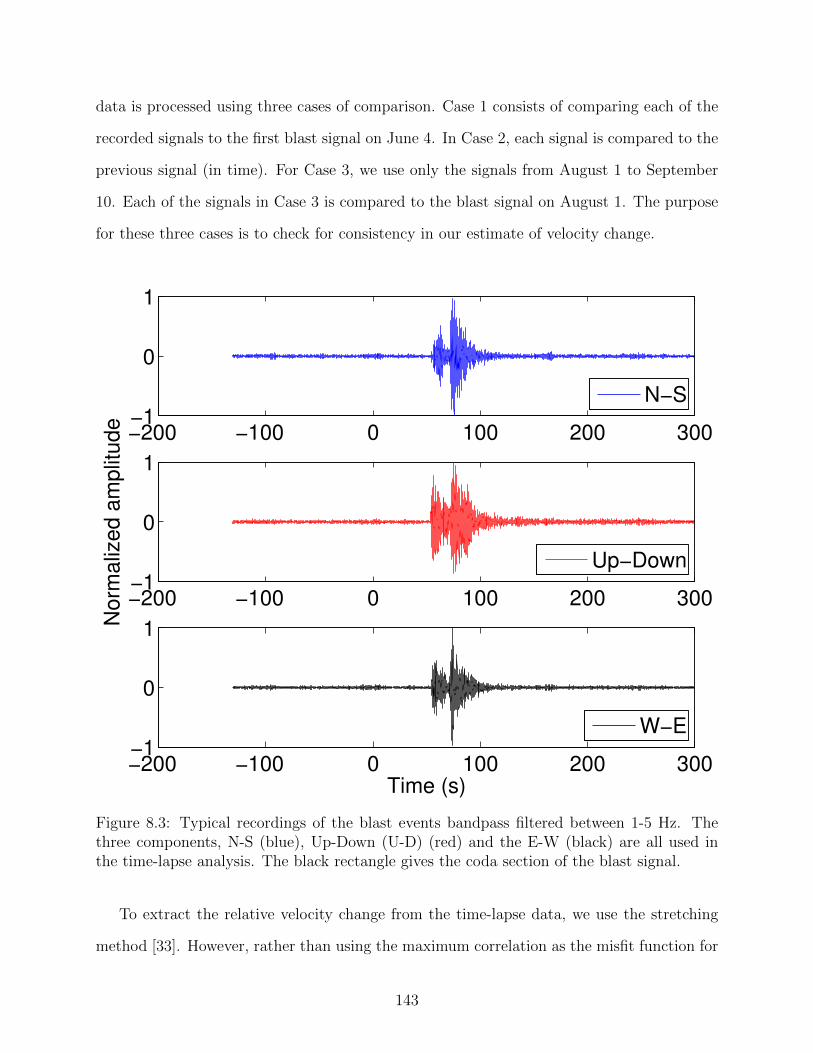
data is processed using three cases of comparison. Case 1 consists of comparing each of the

recorded signals to the first blast signal on June 4. In Case 2, each signal is compared to the

previous signal (in time). For Case 3, we use only the signals from August 1 to September

10. Each of the signals in Case 3 is compared to the blast signal on August 1. The purpose

for these three cases is to check for consistency in our estimate of velocity change.

−200 −100 0 100 200 300−1

0

1

N−S

−200 −100 0 100 200 300−1

0

1

No

rma

lize

d a

mp

litu

de

Up−Down

−200 −100 0 100 200 300−1

0

1

Time (s)

W−E

Figure 8.3: Typical recordings of the blast events bandpass filtered between 1-5 Hz. Thethree components, N-S (blue), Up-Down (U-D) (red) and the E-W (black) are all used inthe time-lapse analysis. The black rectangle gives the coda section of the blast signal.

To extract the relative velocity change from the time-lapse data, we use the stretching

method [33]. However, rather than using the maximum correlation as the misfit function for

143

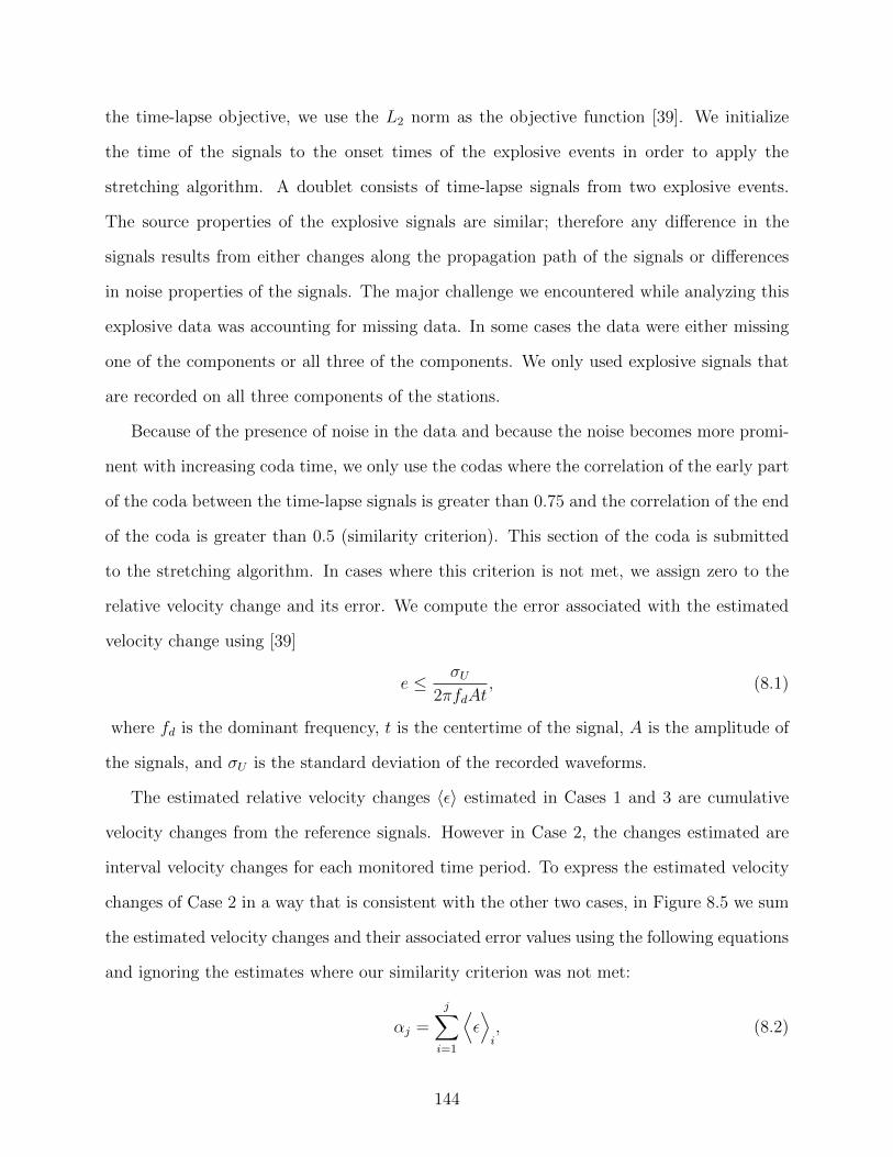
the time-lapse objective, we use the L2 norm as the objective function [39]. We initialize

the time of the signals to the onset times of the explosive events in order to apply the

stretching algorithm. A doublet consists of time-lapse signals from two explosive events.

The source properties of the explosive signals are similar; therefore any di↵erence in the

signals results from either changes along the propagation path of the signals or di↵erences

in noise properties of the signals. The major challenge we encountered while analyzing this

explosive data was accounting for missing data. In some cases the data were either missing

one of the components or all three of the components. We only used explosive signals that

are recorded on all three components of the stations.

Because of the presence of noise in the data and because the noise becomes more promi-

nent with increasing coda time, we only use the codas where the correlation of the early part

of the coda between the time-lapse signals is greater than 0.75 and the correlation of the end

of the coda is greater than 0.5 (similarity criterion). This section of the coda is submitted

to the stretching algorithm. In cases where this criterion is not met, we assign zero to the

relative velocity change and its error. We compute the error associated with the estimated

velocity change using [39]

e �U

2⇡fd

At, (8.1)

where fd

is the dominant frequency, t is the centertime of the signal, A is the amplitude of

the signals, and �U

is the standard deviation of the recorded waveforms.

The estimated relative velocity changes h✏i estimated in Cases 1 and 3 are cumulative

velocity changes from the reference signals. However in Case 2, the changes estimated are

interval velocity changes for each monitored time period. To express the estimated velocity

changes of Case 2 in a way that is consistent with the other two cases, in Figure 8.5 we sum

the estimated velocity changes and their associated error values using the following equations

and ignoring the estimates where our similarity criterion was not met:

↵j

=jX

i=1

D✏E

i

, (8.2)

144

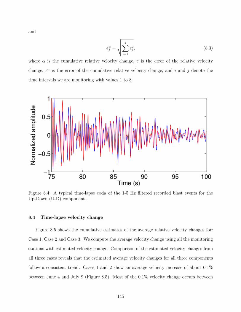
and

e↵j

=

vuutjX

i=1

e2i

, (8.3)

where ↵ is the cumulative relative velocity change, e is the error of the relative velocity

change, e↵ is the error of the cumulative relative velocity change, and i and j denote the

time intervals we are monitoring with values 1 to 8.

Figure 8.4: A typical time-lapse coda of the 1-5 Hz filtered recorded blast events for theUp-Down (U-D) component.

8.4 Time-lapse velocity change

Figure 8.5 shows the cumulative estimates of the average relative velocity changes for:

Case 1, Case 2 and Case 3. We compute the average velocity change using all the monitoring

stations with estimated velocity change. Comparison of the estimated velocity changes from

all three cases reveals that the estimated average velocity changes for all three components

follow a consistent trend. Cases 1 and 2 show an average velocity increase of about 0.1%

between June 4 and July 9 (Figure 8.5). Most of the 0.1% velocity change occurs between

145

June 26 and July 9. The temporal variation of the rest of the velocity changes lie within

the error level of the velocity change. The error values are the standard deviations of the

mean estimated velocity changes from all the stations. However, the velocity remains fairly

constant from July 9 until August 1. Given the consistency in the average velocity changes

after August 1 shown by all the cases, the estimated velocity changes might be significant.

But the variability of these velocity changes is hard to discern given the error level of the

velocity changes.

8.4.1 Spatial distribution of velocity change

Figure 8.6 and Figure 8.7 show the velocity change for each station. The trend of the

velocity changes in these figures are similar to what are observed in the average velocity

changes computed using all the stations. The estimated velocity changes in Figure 8.6

and Figure 8.7 are the estimated velocity changes in Case 2 for each time-lapse period.

Figure 8.6 shows the spatial distribution of the velocity changes which varies with receivers;

the region of dominant velocity changes also varies from one time period to the other.

The estimated velocity changes generally decrease with increasing source-receiver distance

(Figure 8.7). The dependence of the estimated velocity change on the source-receiver distance

explains the high error levels in the average of the estimated velocity change shown in

Figure 8.5. The spread in the velocity changes estimated at the stations is not due to random

errors but due to variations in the estimated velocity change among di↵erent source-receiver

pairs. The spatial distribution of the velocity changes and the dependence of the velocity

change on the source-receiver distance might suggest that the velocity changes in the medium

are spatially localized.

8.4.2 Coda time window analysis of h✏i

Obermann et al. [67] shows that the variation of the estimated velocity change with time

in the coda waves can be use to di↵erentiate between subsurface velocity change at shallow

or at great depths. We estimate velocity change within 5 coda time windows: [ts

; ts

+ 3],

146

Figure 8.5: The cumulative relative velocity changes expressed in percentages for N-S (red),Up-Down (U-D) (green) and the E-W (black) components. Here the average is computedusing all the stations in the USArray displayed in Figure 8.1. Missing first five estimates inCase 3 is because only signals from August 1 is processed in Case 3.

147

Figure 8.6: Relative velocity changes in % estimated from the 8 blast doublets using verticalcomponent of the stations. The blue points are the surface stations. The source locationis the point where all the colored lines meet. The color lines are the estimated percentagevelocity changes for each source-receiver pair.

148

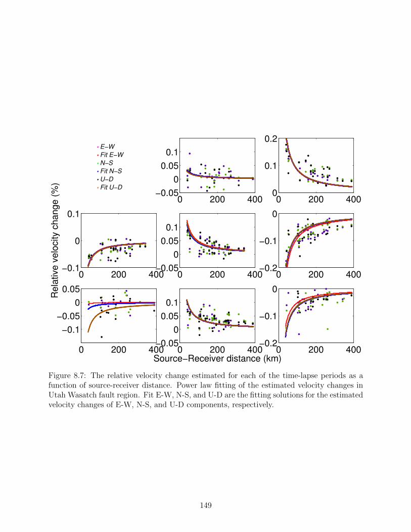
0 200 400−0.05

0

0.05

0.1

0 200 4000

0.1

0.2

0 200 400−0.1

0

0.1

Re

lativ

e v

elo

city

ch

an

ge

(%

)

0 200 400−0.05

0

0.05

0.1

0 200 400−0.2

−0.1

0

0 200 400

−0.1

−0.05

0

0.05

0 200 400−0.05

0

0.05

0.1

Source−Receiver distance (km)0 200 400

−0.2

−0.1

0

. E−W

. Fit E−W

. N−S

. Fit N−S

. U−D

. Fit U−D

Figure 8.7: The relative velocity change estimated for each of the time-lapse periods as afunction of source-receiver distance. Power law fitting of the estimated velocity changes inUtah Wasatch fault region. Fit E-W, N-S, and U-D are the fitting solutions for the estimatedvelocity changes of E-W, N-S, and U-D components, respectively.

149

Figure 8.8: Estimated velocity change di↵erence �T

for each time-lapse period. The plotsshow the estimated velocity change di↵erence �

T

versus the source-receiver distance for theA: N-S component, B: Up-Down (U-D) component, and C: N-S component.

150

Figure 8.9: Estimated velocity change h✏i versus time in the coda for each time-lapse periodusing the N-S component (top), the Up-Down (U-D) component (middle), and the E-Wcomponent (bottom).

151

[ts

+ 5; ts

+ 8], [ts

+ 10; ts

+ 13], [ts

+ 15; ts

+ 18], and [ts

+ 20; ts

+ 23], where ts

is the first

arrival time of the S-wave and the units are seconds. Figure 8.8 shows estimated velocity

change di↵erence �T

for the three signal components - N-S, E-W, and U-D components. We

define the estimated velocity change di↵erence �T

as

�T

= |h✏i|T

� |h✏i|[ts

;ts

+3] (8.4)

where, T is the coda time windows ([ts

+ 5; ts

+ 8], [ts

+ 10; ts

+ 13], [ts

+ 15; ts

+ 18], and

[ts

+ 20; ts

+ 23] seconds). Figure 8.8 compares �T

for all the monitoring stations and time-

lapse periods. We compute the errors using equation 8.3. The figure shows that the velocity

change di↵erences �T

are predominately negative for stations less than 50 km but for source-

receiver distances greater than 50 km the �T

values cluster around zero. The predominately

negative values of �T

for source-receiver distances less than 50 km shows that the absolute

value of the estimated velocity change for the coda times 5 s greater than the arrival time

of S-wave (ts

) are predominately smaller than the absolute value of the estimated velocity

change at the coda time close to the arrival time of S-wave for these distances. These negative

values of �T

for source-receiver distances less than 50 km might indicate that the subsurface

velocity change extends to the near surface [67]. However, the cluster of the �T

values for

source-receiver distances greater than 50 km shows no consistent variations in �T

. This is

because the estimated velocity change is fairly constant across the coda times. Figure 8.9

shows the estimated velocity change across the coda for the three signal components using

station N12A. We estimate the velocity change using 3 s time windows with 2 s overlap. The

overlap allows for more estimates of the velocity changes. The estimated velocity change is

fairly constant across the coda. This variation of the estimated velocity change might suggest

a broad subsurface velocity change across the crust extending to the near-surface.

8.4.3 Parameter Estimation

Assuming a di↵usion model for the coda waves, the traveltime shifts (and therefore

the estimated velocity changes) depend on the magnitude of the subsurface in-situ velocity

152

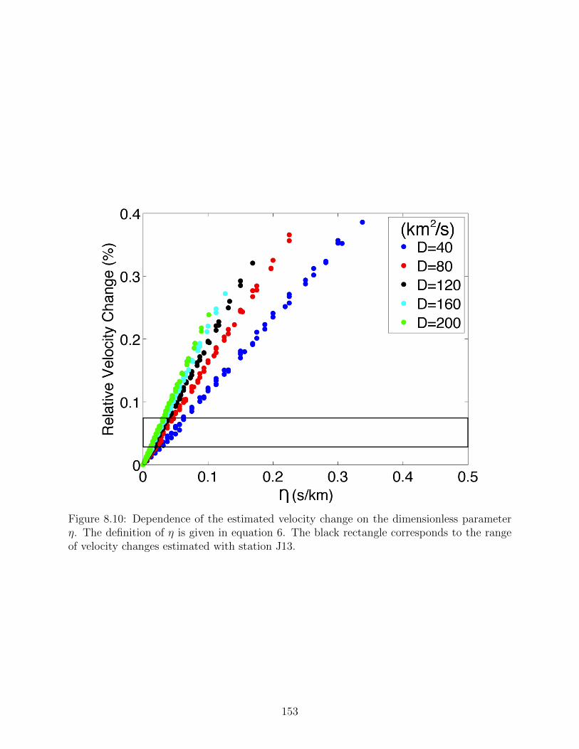
Figure 8.10: Dependence of the estimated velocity change on the dimensionless parameter⌘. The definition of ⌘ is given in equation 6. The black rectangle corresponds to the rangeof velocity changes estimated with station J13.

153

change �v, the volume of the velocity change �V , the di↵usion coe�cient D of the scattered

wave intensity [70], and the source-receiver distance Rsr

. Assuming a uniform lateral velocity

change within a layer of thickness h near the earth’s free surface and 3D bulk wave scattering,

we can formulate the parametric dependence of the estimated relative velocity change h✏i as

follows:

h✏i = F (�v/v, h,D,Rsr

). (8.5)

The function F can be found from the theory of Pacheco and Snieder [70], which relates

the estimated relative velocity change h✏i to the model parameters (�v/v, h,D,Rsr

) through

the relation:

h✏i =Z

V

K(r, t;D)�v

v(r) dV ; (8.6)

where K(r, t;D) is the sensitivity kernel of velocity change using multiply scattered waves,

with travel time t, to subsurface relative velocity change �v/v at location r. Here, the

source-receiver distance Rsr

is given by the known source and receiver locations. For a given


, the estimated relative velocity change depends mostly on the

parameter ⌘, defined as

⌘ =h

D

�v

v. (8.7)

Figure 8.10 shows the apparent (estimated) velocity changes using the source-receiver dis-

tance of station J13 for values of ⌘ from 0 s/km to 0.45 s/km as obtained from equa-

tion 8.5. These values of ⌘ cover the range of relative velocity change we observe in this

study (h✏i < 0.2%). Figure 8.10 suggests that the combined e↵ect of the magnitude of the

subsurface velocity change �v and the depth of the velocity change h have the greatest influ-

ence on the estimated velocity change, for a given source-receiver distance Rsr

. Assuming the

di↵usion model, di↵erent D values gives di↵erent slopes in Figure 8.10. With a wide range

of estimated velocity change h✏i, these di↵erent slopes suggest that di↵usion coe�cient D

gives a weaker trade-o↵ with the other two parameters, the magnitude of subsurface relative

154

velocity change �v/v and the depth of velocity change h. However, for the range of velocity

change we estimate in this study (black rectangle in Figure 8.10 for station J13), the depen-

dence of h✏i on the three parameters (h, D, �v/v) is mostly through the combination of ⌘.

We cannot separate the e↵ect of D except if we independently estimate D. Figure 8.10 is for

Station J13, the other stations show a similar trade-o↵ between the three model parameters.

We can constrain the di↵usion coe�cient D by using the relationship that at the peak of

the coda intensity, D = R2sr

/6hti (Appendix E). The weighted average time hti corresponds

to the peak of the coda intensity. For the current dataset, the estimated average di↵usion

coe�cient is 106 km2/s. Fixing the di↵usion coe�cient to this average value, the velocity

change is a function of the trade-o↵ between �v/v and h. The trade-o↵ between �v/v and h

makes it impossible to independently determine each of these parameters without additional

information.

According to equation E.12 in Appendix E, we can use a power law relation to describe

the dependence of estimated velocity changes on distance (Figure 8.7) as:

h✏i = aR�1sr

, (8.8)

where a = (h�v/v)⌃ (equation A12). ⌃ is a dimensionless constant of the monitored region

(equation E.11) that depends on the di↵usion coe�cient D. Using the power-law relation in

equation 8.8, we invert the values of h�v/v from the estimated velocity changes. Table 8.1

gives the estimated parameters for the fitting solutions of the estimated velocity changes,

the goodness of fit in R2 (a measure of regression) values, and the inverted values of h�v/v.

We use the weighted nonlinear least-squares method with the inverse of the estimated errors

as weights. Negative R2 values are encountered due to the use of a nonlinear model [18].

Based on the surface layer model, the inverted values for h�v/v are of the order of 1 %km

(Table 8.1). This value of h�v/v implies, for a change extending throughout the crustal

thickness of 25-40 km, the average subsurface in-situ velocity becomes less than 0.04%.

However, when the thickness of the layer is limited to less than a kilometer the velocity

change is large (' 1%). A velocity change of less than 0.04% for a crustal-scale deformation

155

might be realistic in the actively extending Basin and Range province.

The di↵usion model in the Appendix E generally explains the decrease of the estimated

velocity changes h✏i with the source-receiver distance. However, as the goodness of fit in

R2 indicates (Table 8.1), equation E.12 provides a poor description of the variation of the

estimated velocity changes h✏i with source-receiver distance. This poor fit results from the

significant scatter in the estimated velocity changes h✏i. The deviation of the estimated

velocity changes h✏i from equation E.12 can result from heterogeneity in the scattering

properties of the monitored subsurface (captured by varying D values) or heterogeneity

in the subsurface velocity change. These heterogeneity are ignored in the di↵usion model in

Appendix E.

8.5 Causes for the velocity changes

Variations in subsurface velocity at time scales similar to the ones in the observed velocity

changes might be induced by fluctuations in seasonal stress loading including precipitation,

hydrological cycles, thermal changes, local seismicity, and groundwater level variations [104].

8.5.1 Seasonal loading

Utah is a region that receives little precipitation. Available precipitation records for the

monitored region show that the cumulative precipitation during the monitored time period

is less than 5 cm. This amount of precipitation can not induce the amount of velocity change

observed. The groundwater level, however, can vary temporally, not only due to precipitation

but also to irrigation practices [6], stress loading resulting from large earthquakes [60], and

solid earth tides [100]. Figure 8.11 shows the correlation between cumulative groundwater

level change (positive values corresponds to deepening of the groundwater level) over the

monitored period with the estimated average velocity change from Case 2, using 9 recording

wells. The location of the recording wells of the groundwater level are shown in Figure 8.1.

For a few of the wells (wells S4, S7, S8 and S9), a linear regression suggests that the average

velocity changes show significant correlation (with regression coe�cients R2 > 0.5) with

156

0 0.2 0.4−0.05

0

0.05

0.1

0.15

Groundwater level change (m)

Ve

loci

ty c

ha

ng

e (

%)

0 5 10−0.05

0

0.05

0.1

0.15


Ve

loci

ty c

ha

ng

e (

%)

0 2 4−0.05

0

0.05

0.1

0.15


Ve

loci

ty c

ha

ng

e (

%)

0 0.5 1−0.05

0

0.05

0.1

0.15


Ve

loci

ty c

ha

ng

e (

%)

0 0.2 0.4−0.05

0

0.05

0.1

0.15


Ve

loci

ty c

ha

ng

e (

%)

0 5 10−0.05

0

0.05

0.1

0.15

Groundwater level change (m)V

elo

city

ch

an

ge

(%

)

−0.1 −0.05 0−0.05

0

0.05

0.1

0.15


Ve

loci

ty c

ha

ng

e (

%)

0 0.05 0.1−0.05

0

0.05

0.1

0.15


Ve

loci

ty c

ha

ng

e (

%)

0 0.5 1−0.05

0

0.05

0.1

0.15


Ve

loci

ty c

ha

ng

e (

%)

E-WN-SU-D

E-WN-SU-D

E-WN-SU-D

E-WN-SU-D

E-WN-SU-D

E-WN-SU-D

E-WN-SU-D

E-WN-SU-D

E-WN-SU-D

S1 S2 S3

S4 S5 S6

S7 S8 S9

Figure 8.11: Correlation of average velocity change with groundwater level change measuredin meters (positive meters mean deepening of the groundwater level). Each plot shows thefit of the average velocity changes from the three signal components. S1 to S9 are the namesof the groundwater wells.

157

the groundwater level subsidence. We quantify the quality of the correlation using the

R2 values of the linear fit (Table 8.2) [23]. We obtain R2 values less than 0.67 using a

weighted least-squares fit, where we use the standard deviation of the estimated velocity

change as the weights. Among wells S4, S7, S8 and S9, only well S7 supports a direct

proportional relationship between velocity change and stress (pressure) changes, if we assume

that increase in groundwater level change results in an increase in e↵ective stress. The

maximum groundwater level change within the time period monitored among the wells is

less than 2 m. This corresponds to approximately a change in the e↵ective stress of less than

2.94 x 10�2 MPa assuming that the Biot coe�cient is equal to 1 and a soil density of less

than 2.5 g/cm3. The stress sensitivity ⌘ reported in the literature is between 10�6/Pa and

10�9/Pa [44, 94]. These stress sensitivity values imply a range of �v/v values of magnitude

10�2 to 10�5 %. Given that these values of �v/v are orders of magnitude smaller than the

estimated velocity changes h✏i and that only a few of the stations show significant positive

correlation with the velocity changes (Figure 8.11), the groundwater level change is unlikely

to explain the observed velocity changes.

Seasonal strain changes can be recorded by detrended GPS displacement measurements.

Using horizontal GPS displacements from GPS stations within our monitored region (Fig-

ure 8.1), we quantify the correlation between the estimated relative velocity change and

the seasonal E-W strain using the R2 values of the linear fit (Figure 8.12). We compute

the average horizontal strain between stations using the average detrended horizontal GPS

displacements denoted by di,jk

. Because, the horizontal distances between the stations are

much larger than the elevations between the stations, we approximate the average horizontal

strains by:

�ijkk

=djk

� dik

Xj

k

�X i

k

, (8.9)

where, i and j are station indexes, Xk

is either E-W (k = 1) or N-S (k = 2) GPS location,

and � is the average strain. The detrended GPS displacement di,jk

is averaged two days prior

158

0 5 10 15

x 10−9

−0.1

−0.05

0

0.05

0.1

Ve

loci

ty c

ha

ng

e (

%)

1 1.5 2 2.5 3

x 10−8

−0.1

−0.05

0

0.05

0.1

0 1 2 3

x 10−8

−0.1

−0.05

0

0.05

0.1

−2 0 2 4

x 10−9

−0.1

−0.05

0

0.05

0.1

E-W

N-S

U-D

E-W

N-S

U-D

E-W

N-S

U-D

E-W

N-S

U-D

A

B

C

D

Ve

loci

ty c

ha

ng

e (

%)

Ve

loci

ty c

ha

ng

e (

%)

Ve

loci

ty c

ha

ng

e (

%)

Mean Strain (E−W)

Figure 8.12: Linear regression between the E-W strain derived from E-W GPS detrendeddisplacement and the individual components of average velocity change (E-W, N-S, andvertical components). The linear regression is computed using A, all the available GPSdisplacement, B, only the Basin and Range GPS displacements, C, only the Wasatch faultdisplacements, and D, only the Snake River Plain GPS displacements.

159

to and two days after the time of each blast. Table 8.3 and Figure 8.12 show the linear

correlation with the estimated average velocity changes using 4 groups of the GPS stations.

One group consists of all the available GPS stations while the other 3 groups use either only

stations within the Snake River Plain, only stations within the Basin and Range, or only the

stations close to the Wasatch fault. Comparison of the estimated average velocity changes

from Case 2 with the average horizontal GPS strain using all the GPS stations shows a

significant linear correlation, based on the R2 values, of the velocity changes with the East-

West strain (Table 8.3). For the strains derived from the Basin and Range GPS stations,

there is a larger correlation of the velocity changes with the East-West strains compared

to the strain derived from all the stations. Stations along the Snake River Plain region

show negligible correlation (R2 < 0.23) with the observed velocity change (Figure 8.12D,

and Table 8.3). Fits with negative R2 values here, suggests that the linear fit might be an

incorrect model for those fits.

Seasonal variation in GPS displacement and therefore the seasonal variations in the strain

can be induced by thermoelastic or hydrologic variations [104]. While hydrologic variations

can induce localized changes, variations in the thermal conditions within the crust can be

responsible for a broad crustal deformation [42]. Crustal deformation in the Basin and Range

predominately creates normal fault and extensive structures striking in approximately north-

south orientations. The correlation between the estimated average velocity changes and the

calculated strain changes suggests that the velocity changes might be driven at least in part

by the changes in the seasonal strain. With the inconsistent correlation we obtained between

the average velocity and the groundwater level change, the strain changes here, might be

driven by tectonic or thermoelastic stress changes. Given that the observed velocity changes

correlate significantly with the strains aligned in the direction of the crustal deformation in

the area, the velocity changes we observe might extend deep into the crust and therefore

result in a small subsurface �v/v. If the seasonal strains from the Basin and Range GPS

detrended displacements are induced by crustal deformation, a significant part of the velocity

160

change observed might be driven by broad crustal deformation in the monitored region. The

monitored region covers the eastern flank of the Basin and Range, which has been shown to

have elevated thermal conditions [24] that might be responsible for broad active deformation

in the region. Tectonic deformation of the region could induce velocity changes within the

crust; however, these velocity changes are broader, more gradual, and extend deeper than the

change due to other physical mechanisms such as variations in groundwater level or regional

seismicity. Because of the broad and gradual properties of the crustal deformation-induced

velocity changes, we expect larger values of h (volume of change) and lower subsurface

relative velocity changes �v/v. With a larger value of h, crustal deformation due to stress

changes or elevated temperatures deep within the crust might explain, at least in part, the

inverted values of h�v/v on the order of 1%km.

8.5.2 Local seismicity

Figure 8.13 shows the peak ground acceleration (PGA) due to local seismicity and the es-

timated velocity changes. We compute PGA (y) using its relationship with event magnitude

given by Chiou et al. [17]:

ln(y) = ln(yref

) + � ln(Vs30) + f

NL

(Vs30, yref ) (8.10)

where ln (yref

) = c1 � 2.1 ln[Rf

+ CNS

] + (�0.5 + 2.1) lnpR

f

+ 502 + �Rf

and CNS

=

c5 cosh[c6max(M � 3.0)]. Vs30 is the average shear wave velocity in the top 30m, f

NL

defines

the nonlinear soil response of the monitored area, M is the event magnitude, and Rf

is

the distance to the fault rupture location in km. We use values for coe�cients �, �, c1,

c5, and c6 reported by Pankow [73] for the Utah region. To compute PGA, we use the

Vs30 value of 230m/s. The deviation of V

s30 for each monitoring station from 230m/s will

a↵ect the magnitude of the PGA values and will a↵ect negligibly the temporal variations

of the PGA values. The temporal variations of the PGA values depends on the number

and magnitude of the seismicity registered during each time period. We compute PGA for

earthquake magnitudes and hypocenter parameters determined by the Utah Regional Seismic

161

Figure 8.13: Comparison of the peak ground acceleration (PGA) with average relative ve-locity change estimated in Case 2. The PGA values are estimated from the local seismicity(M > -0.36) that occurred during the monitored time-lapse period. The PGA values areestimated using relationship between PGA and the magnitude of an earthquake Chiou et al.[17].

162

Network for seismic events in the monitoring region during the monitored time-lapse period

(Figure 8.1).

The following time intervals contain days of relatively high spikes of PGA events: August

1 - August 6, August 13 - August 27, and August 27 - September 10 (Figure 8.13). Among

these time periods, only the time period – August 27 - September 10 – has the anomalous

PGA events occurring near the end of each time-lapse period. Comparing the PGA values

with the estimated average velocity change, there is no clear correlation between the local

seismicity induced PGA and the estimated average velocity changes. This insignificant cor-

relation is suggested by the R2 value of the linear fit between the PGA (total and average)

values and the estimated average velocity changes (Table 8.4). The R2 value of the linear fit

for each of the average velocity changes is less than 0.32.

The e↵ect of the local seismicity is expected to be constrained near the Wasatch fault

which is situated in the eastern section of the monitored region. Therefore, local seismicity

within the Wasatch fault system might be an unlikely cause for the observed velocity changes.

8.6 Discussion and Conclusions

The estimated velocity changes suggest that the eastern flank of the Basin and Range

and the transition to the Middle Rocky Mountains and Colorado Plateau, are undergoing

small but significant velocity changes within a short period of time. Correlation of the

estimated velocity changes with groundwater level changes, seasonal tectonic strain changes

and local seismicity indicates that the velocity change mostly might be induced by the East-

West crustal deformation in the eastern Basin and Range. The magnitude of the estimated

average velocity change varies from one time-lapse period to the other. The maximum of the

absolute value of the estimated velocity change is 0.2%. Due to the averaging e↵ect of coda

interferometry, the volume and the magnitude of the velocity change are strongly correlated.

We observe that the path-averaged velocity changes depend on the distance between the

monitoring source and receivers. The estimated velocity changes generally decrease with


. This reduction in the estimated velocity change with source-

163

receiver distance is seen assuming 3D di↵usion wave scattering. With the di↵usion model and

assuming a uniform scattering model, there is an inverse Rsr

dependence of the estimated

velocity changes h✏i. However, there is significant deviation of the estimated velocity changes

h✏i from the inverse Rsr

relation. This deviation can result from heterogeneities in the

subsurface �v/v or in the scattering properties of the subsurface. To obtain the inverse Rsr

relation and consequently estimate the magnitude of the subsurface in-situ velocity change

using the coda waves, we have made the following simplifying assumptions:

First, we assume that the coda waves we use for the time-lapse monitoring are described

using the di↵usion approximation for multiply scattered waves. This approximation is usu-

ally an over-simplification of the scattered waves especially in the early part of the coda.

This approximation is likely to result in an erroneous estimation of the inverted values of

h�v/v. Also we assume a uniform di↵usion model for the monitored area defined by an av-

erage di↵usion constant in the subsurface. This di↵usion constant is related to the distance

between source and receivers using the di↵usion model of the recorded intensities. If the

average di↵usion constant is uncharacteristic of the variation of the di↵usion property of the

monitored region, the inverted h�v/v will also be erroneous.

Second, we use a semi-infinite 3D subsurface with a fully reflecting free surface to in-

vert for h�v/v. The fully reflecting free surface may be a fair approximation of the free

surface, but we ignore the presence of the Moho discontinuity. This boundary will change

the magnitude of the sensitivity kernel of the coda because the crustal thickness is much

less than the source-receiver distances used in estimating the velocity changes. Keller et al.

[40] suggest that the crustal Basin and Range-Colorado Plateau transition has a thickness of

about 25 km with a crustal thickness of 30 km for the Basin and Range [29]. Assuming an

absorbing boundary at the crust-upper mantle interface will likely increase the magnitude

of the sensitivity kernel [82]. Figure 8.14 shows that with a Moho interface at 25 km, the

volumetric integral of the sensitivity kernel is increased by a factor of 1.25 to 1.80 depending

on the source-receiver distance. This will result in a reduction of the value of the inverted

164

0 50 100 150 200 250 300 350 400

1.3

1.4

1.5

1.6

1.7

1.8

1.9

Ra

tio v

olu

me

inte

gra

l of th

e s

en

sitiv

ity k

ern

el (

s)

source−receiver distance (km)

Figure 8.14: Increased sensitivity due to the presence of Moho interface at depth 25kmbased on the ratio of the volume integral of the sensitivity kernel with and without theMoho interface.

165

h�v/v.

Third, we made a 2D approximation of the expression of Pacheco and Snieder [70] in

equation E.6 by assuming that h/Rsr

⌧ 1. Therefore, the inverted h�v/v represents the

true h�v/v within the subsurface if the velocity changes are restricted within the crust. If

the observed velocity changes result from a deeper region of the subsurface, then the true

values of h�v/v might deviate from the inverted values. Because of the large values of Rsr

(several hundred kms), the approximation of h/Rsr

⌧ 1 is not likely to significantly a↵ect

the inverted values of h�v/v.

Fourth, due to the extent of the monitored region, the recorded explosive signals are

expected to generate surface waves. Due to conversion from body waves to surface waves,

the surface waves can arrive within the coda wave time window especially for short source-

receiver distances. In the recorded explosive signals, the surface waves mostly arrive after

the coda waves. However, the relative arrival times of the coda wave and the surface wave

are dependent on the source-receiver distances. In this study we have restricted the velocity

changes analysis to the coda wave. The variation of the estimated velocity change across the

coda (Figure 8.9) does not suggest a significant presence or contribution of surface-dominated

scattered wave [67]. However, the presence of surface wave or surface dominated scattered

waves in the coda will increase the sensitivity of the scattered waves to localized velocity

change. This will result in lower values of h�v/v. Therefore the inverted h�v/v values can

be considered as the upper limit of the real h�v/v changes within the monitored region.

Finally, we assume a uniform lateral velocity change in the layer of velocity change across

the monitored region. In reality it is likely that the velocity changes are localized in space

both laterally and in depth. A heterogeneity in the subsurface velocity change likely explains

the scatter in the estimated velocity changes. The inverted h�v/v can be seen as the average

h�v/v of the true h�v/v within the monitored region. This means that in some areas of

the monitored region the true changes will be higher or lower than the inverted values.

166

The above assumptions notwithstanding, the estimated velocity changes suggest that

the crust underneath the region around the eastern Basin and Range is undergoing a path-

averaged velocity change of the order of 0.1% within a short period of time. There might be a

need to incorporate these velocity changes in any characterization of both the seismicity and

deformation within the region. However, it would be useful to discern if these velocity changes

are seasonal by incorporating measurements taken over several years or by applying coda

wave interferometry to the coda waves generated from ambient noise correlations [33, 89].

8.7 Acknowledgments

We are grateful for the financial support of the Department of Energy (DOE) through

grant DE-EE0002758. The explosive signals used in this study were obtained from the

broadband USArray stations via IRIS.

167

Table 8.1: Estimated model parameters using the inverse R relation.

Event period a (%km) R2 h�v

v

(%km)Period 1 (06/04-06/26)E-W 1.208 ± 4.6796 -0.0359 0.2796 ± 1.0830N-S 1.227 ± 4.0842 -0.0244 0.2840 ± 0.9452U-D 1.069 ± 4.9240 -0.02897 0.2474 ± 1.1396Period 2 (06/26-07/09)E-W 8.272 ± 0.6536 0.3448 1.9144 ± 0.1514N-S 8.358 ± 0.8643 -0.0987 1.9343 ± 0.2001U-D 8.450 ± 1.1125 -0.3393 1.9556 ± 0.2576Period 3 (07/09-07/16)E-W -3.382 ± 0.3990 0.2096 -0.7827 ± 0.0924N-S -3.502 ± 0.4276 -0.0120 -0.8105 ± 0.0990U-D -3.574 ± 0.5839 -0.2823 -0.8271 ± 0.1352Period 4 (07/16-08/01)E-W 4.677 ± 0.3941 0.4538 1.0824 ± 0.0913N-S 4.141 ± 0.4903 -0.3588 0.9584 ± 0.1135U-D 4.382 ± 0.4513 0.2150 1.0141 ± 0.1045Period 5 (08/01-08/06)E-W -9.001 ± 0.6926 0.09855 -2.0831 ± 0.1605N-S -8.038 ± 0.5898 0.2633 -1.8602 ± 0.1366U-D -7.889 ± 0.8625 -0.0293 -1.8258 ± 0.1997Period 6 (08/06-08/13)E-W -0.2111 ± 7.7143 0.00313 -0.0489 ± 1.7853N-S -0.9408 ± 6.9643 -0.0524 -0.2177 ± 1.6117U-D -4.062 ± 33.2908 0.1378 -0.9401 ± 7.7045Period 7 (08/13-08/27)E-W 4.003 ± 0.5133 -0.3547 0.9264 ± 0.1188N-S 3.949 ± 0.6128 -1.569 0.9139 ± 0.1418U-D 4.019 ± 0.4722 0.06362 0.9301 ± 0.1093Period 8 (08/27-09/10)E-W -5.143 ± 0.9411 0.118 -1.1902 ± 0.2178N-S -6.538 ± 0.9513 -0.0716 -1.5131 ± 0.2202U-D -6.328 ± 3.2270 -0.2798 -1.4645 ± 0.7469

168

Table 8.2: Goodness of fit between average relative velocity changes and groundwater (GWL)subsidence based on the R2 value (Case 2).

Velocity Compo-nents /

S1 S2 S3 S4 S5 S6 S7 S8 S9

GWL stationsE-W -0.1866 0.0367 0.3931 0.4412 0.3179 0.1779 0.5178 0.4376 0.4798N-S -0.1858 0.1071 0.4697 0.4743 0.3641 0.2612 0.5366 0.5125 0.5274U-D -0.2493 0.0297 0.3706 0.6005 0.4117 0.2057 0.6658 0.6142 0.6357

Table 8.3: Goodness of fit between average relative velocity changes and seasonal variationof (detrended) GPS displacement based on the R2 value (Case 2).

GPS Component / Velocity Components E-W N-S U-DAll GPS stationsE-W 0.6106 0.5228 0.4993N-S -0.1240 -0.1401 -0.1828Basin and Range stationsE-W 0.7842 0.7982 0.6354N-S -0.1424 -0.1545 -0.1952Wasatch fault stationsE-W 0.6335 0.5442 0.6267N-S 0.1476 0.1912 0.0750Snake River Plain stationsE-W 0.2261 -0.0052 -0.1200N-S -0.1127 -0.1491 -0.0770

Table 8.4: Goodness of fit between relative velocity change and PGA based on the R2 value(Case 2).

Velocity Components Total PGA soil Mean PGA soilE-W 0.2186 -0.0208N-S 0.3158 0.0504U-D 0.2060 0.0472

169

CHAPTER 9

CONCLUSION AND FUTURE WORK

The goal of my thesis work was to study the capability of imaging weak time-lapse changes

and to develop imaging tools to image these changes. The time-lapse changes I considered

range from velocity changes within mechanical and geo-mechanical structures to changes in

the scattering strength of a scattering medium. The studies in the dissertation also focus on

weak changes in which multiply scattered waves tend to provide higher sensitivity than singly

scattered waves. These weak changes include velocity changes within the earth or mechanical

structures which might result from naturally occurring events, induced stress changes, or

thermal forcings. The changes also can result from various types of wear and tear in buildings,

roads, and machines due to aging of these structures or to induced external forcings. The

major contribution of this work is a technique for characterizing and localizing weak changes

within any scattering medium using multiply scattered waves. This contribution extends the

usual focus of coda wave interferometry, which is to detect weak changes within scattering

media without providing significant information on the location of the detected change.

I developed an inversion algorithm that simultaneously detects and images localized weak

changes within a scattering medium. The imaged localized change suggests that the reso-

lution depends on the coda lapse time where the imaging data is extracted and on the

monitoring source and receiver setup. We have explored a few topics in regard to detecting

and imaging changes within a scattering medium such as determining the impact of the shifts

in the properties of the sources generating the repeating coda waves, localizing change within

a statistical heterogeneous medium, and characterizing the sensitivity of acoustic and elastic

scattered waves. There remain a number of unexplored issues regarding the monitoring of

localized weak changes using time-lapse coda waves.

170

There is need to extensively investigate the control that the source and receiver setup has

on the inversion process. In Chapter 5, we show the e↵ect of data averaging, which increases

with coda lapse time, on the imaging process. However, the spread of the estimated change

from the scattered waves across the source-receiver pairs depends on the placement of the

source-receiver pairs relative to the time-lapse change to be imaged. An e↵ective source-

receiver geometry for monitoring includes source-receivers pairs for whom the ballistic waves

traverse the anomaly, as well as source-receiver pairs for which the scattered waves sample the

anomaly. Determining an optimal monitoring source-receiver setup that images a localized

change will require a priori information about the general location of the change (if present)

and about the scattering property of the medium.

In Chapter 4, we demonstrate the computation of the elastic sensitivity kernel and explain

the characteristics of the sensitivity to perturbations in the P- and S-wave velocities. There

is a need to apply these sensitivity kernels to imaging P- and S-wave velocity changes in real

data problems such as those in the laboratory imaging problems found in Chapter 6. Because

of the time constraint, we will leave the imaging with elastic kernels to future studies.

The sensitivity kernel both for acoustic and elastic wave scattering uses the scattered

intensity field rather than the scattered wavefield. Utilizing the scattering intensity field

allows us to formulate the imaging problem when we know only the statistical properties

of the scattering model, without the need to know the precise locations and characteristics

of the microscopic scatterers within the scattering medium. The question for future studies

is, can we reformulate the imaging problem to use the scattered wavefield for computing

the sensitivity kernel without using a priori the microscopic properties of the individual

scatterers present within the scattering medium?

The numerical computation of the sensitivity kernel is dependent on knowledge of the

statistical properties of the scattering medium. For a statistically homogeneous scattering

medium, the scattering properties of the medium can be estimated by fitting and describing

the envelope of the scattered intensity recorded by the receivers. However, for a heteroge-

171

neously scattering medium, more elaborate techniques will be needed to estimate the a priori

scattering model for the kernel computations. We can estimate the a priori scattering model

by describing the envelope of the time lapse coda when a dense monitoring array is present

or by using imaged models from other geophysical imaging techniques such as migration

velocity analysis, full waveform inversion and well-log measurements. For a weak velocity

change and an accurate a priori scattering model, the sensitivity kernel is computed once

and can be reused for subsequent time-lapse monitoring of a given medium. The question

for future studies becomes, What is the impact of an error in the a priori scattering model

on the computed sensitivity kernel and, in general, on the imaging of localized changes?

172

REFERENCES CITED

[1] Aki, K. and L. Chouet, 1975, Origin of coda waves: source, attenuation, and scatteringe↵ects: J. Geophys. Res., 80, 3322–3342.

[2] Aki, K. and P. G. Richards, 2002, Quantitative seismology: University Science Books.

[3] Akkermans, E. and G. Montambaux, 2007, Mesoscopic physics of electrons and photons:Cambridge University Press. Cambridge Books Online.

[4] Arts, R., O. Eiken, A. Chadwick, P. Zweigel, L. Van der Meer, and B. Zinszner, 2004,Monitoring of CO2 injected at Sleipner using time-lapse seismic data: Energy, 29, 1383–1392.

[5] Asano, Y., T. Saito, Y. Ito, K. Shiomi, H. Hirose, T. Matsumoto, S. Aoi, S. Hori, and S.Sekiguchi, 2011, Spatial distribution and focal mechanisms of aftershocks of the 2011 o↵the Pacific coast of Tohoku earthquake: Earth, Planets and Space, 63, 669–673.

[6] Ashland, X. and R. E. Giraud, 2005, Groundwater level fluctuations in Wasatch frontlandslides and adjacent slopes, Northern Utah: Utah Geological Survey Open-File Report,448, 22.

[7] Aster, R. C., B. Borchers, and C. H. Thurber, 2013, Parameter estimation and inverseproblems: Academic Press.

[8] Belkebir, K., P. C. Chaumet, and A. Sentenac, 2006, Influence of multiple scattering onthree-dimensional imaging with optical di↵raction tomography: Journal of the OpticalSociety of America A, 23, 586–595.

[9] Berkhout, A. and D. Verschuur, 2006, Imaging of multiple reflections: Geophysics, 71,SI209–SI220.

[10] Berkhout, A., D. Verschuur, and G. Blacquire, 2012, Illumination properties andimaging promises of blended, multiple-scattering seismic data: a tutorial: GeophysicalProspecting, 60, 713–732.

[11] Bouchon, M., C. A. Schultz, and M. N. Toksz, 1996, E↵ect of three-dimensional topog-raphy on seismic motion: Journal of Geophysical Research: Solid Earth, 101, 5835–5846.

173

[12] Brenguier, F., M. Campillo, C. Hadziioannou, N. Shapiro, and E. Larose, 2008a, Post-seismic relaxation along the San Andreas Fault at Parkfield from continuous seismologicalobservations: Science, 321, 1478–1481.

[13] Brenguier, F., N. M. Shapiro, M. Campillo, V. Ferrazzini, Z. Duputel, O. Coutant, andA. Nercessian, 2008b, Towards forecasting volcanic eruptions using seismic noise: NatureGeoscience, 1, 126–130.

[14] Busch, K., C. M. Soukoulis, and E. N. Economou, 1994, Transport and scattering meanfree paths of classical waves: Physical Review B, 50, 93–98.

[15] Chen, J. H., B. Froment, Q. Y. Liu, and M. Campillo, 2010, Distribution of seismicwave speed changes associated with the 12 May 2008 Mw 7.9 Wenchuan earthquake:Geophysical Research Letters, 37.

[16] Cheng, X., F. Niu, and B. Wang, 2010, Coseismic velocity change in the rupture zoneof the 2008 Mw 7.9 Wenchuan earthquake observed from ambient seismic noise: Bulletinof the Seismological Society of America, 100, 2539 –2550.

[17] Chiou, B., R. Youngs, N. Abrahamson, and K. Addo, 2010, Ground-motion attenuationmodel for small-to-moderate shallow crustal earthquakes in California and its implicationson regionalization of ground-motion prediction models: Earthquake Spectra, 26, 907–926.

[18] Colin Cameron, A. and F. A. Windmeijer, 1997, An R-squared measure of goodness offit for some common nonlinear regression models: Journal of Econometrics, 77, 329–342.

[19] Compton, S. and D. Hale, 2013, Estimating vp

/vs

ratios using smooth dynamic imagewarping: Center for Wave Phenomena, Report 765, 211–222.

[20] Cowan, M. L., I. P. Jones, J. H. Page, and D. A. Weitz, 2002, Di↵using acoustic wavespectroscopy: Physical Review. E, Statistical, Nonlinear, and Soft Matter Physics, 65.PMID: 12188849.

[21] Daley, T., L. Myer, J. Peterson, E. Majer, and G. Hoversten, 2008, Time-lapse crosswellseismic and VSP monitoring of injected CO2 in a brine aquifer: Environmental Geology,54, 1657–1665.

[22] Davis, T. L., M. J. Terrell, R. D. Benson, R. Cardona, R. R. Kendall, and R. Winarsky,2003, Multicomponent seismic characterization and monitoring of the CO2 flood at Wey-burn field, Saskatchewan: The Leading Edge, 22, 696–697.

[23] Draper, N. R. and H. Smith, 1981, Applied regression analysis: Wiley.

174

[24] Eaton, G. P., 1982, The Basin and Range Province: Origin and tectonic significance:Annual Review of Earth and Planetary Sciences, 10, 409–440.

[25] Fichtner, A., F. Bleibinhaus, and Y. Capdeville, 2011, Full seismic waveform modellingand inversion: Springer.

[26] Fleury, C., 2013, Increasing illumination and sensitivity of reverse-time migration withinternal multiples: Geophysical Prospecting, 61, 891–906.

[27] Foldy, L. L., 1945, The multiple scattering of waves. I. General theory of isotropicscattering by randomly distributed scatterers: Physical Review, 67, 107–119.

[28] Gaburro, R., C. J. Nolan, T. Dowling, and M. Cheney, 2007, Imaging from multiplyscattered waves: Society of Photo-Optical Instrumentation Engineers, 304–311.

[29] Gilbert, H. J. and A. F. Sheehan, 2004, Images of crustal variations in the intermountainwest: Journal of Geophysical Research: Solid Earth, 109, B03306.

[30] Godano, M., T. Bardainne, M. Regnier, A. Deschamps, and M. Valette, 2012, Spatialand temporal evolution of a microseismic swarm induced by water injection in the Arkema-Vauvert salt field (southern France): Geophysical Journal International, 188, 274–292.

[31] Gret, A., R. Snieder, and U. Ozbay, 2006, Monitoring in situ stress changes in a miningenvironment with coda wave interferometry: Geophysical Journal International, 167, 504–508.

[32] Groenenboom, J., 1995, Attenuation, dispersion, and anisotropy by multiple scatteringof transmitted waves through distributions of scatterers: The Journal of the AcousticalSociety of America, 98, 3482–3492.

[33] Hadziioannou, C., E. Larose, O. Coutant, P. Roux, and M. Campillo, 2009, Stabilityof monitoring weak changes in multiply scattering media with ambient noise correlation:Laboratory experiments: Journal of the Acoustical Society of America, 125, 3688–3695.

[34] Hale, D., 2013, Dynamic warping of seismic images: Geophysics, 78, S105–S115.

[35] Hale, D. and S. Compton, 2013, Smooth dynamic warping: Center for Wave Phenom-ena, Report 764, 201–210.

[36] Haney, M. M., K. van Wijk, and R. Snieder, 2005, Radiative transfer in layered mediaand its connection to the O’Doherty-Anstey formula: Geophysics, 70, T1–T11.

175

[37] Hennino, R., N. Tregoures, N. Shapiro, L. Margerin, M. Campillo, B. Van Tiggelen, andR. Weaver, 2001, Observation of equipartition of seismic waves: Physical Review Letters,86, 3447–3450.

[38] Kanu, C. and R. Snieder, 2014, Numerical computation of the sensitivity kernel fortime-lapse monitoring with multiply scattered waves: Center for Wave Phenomena, Re-port 816, 291–306.

[39] Kanu, C. O., R. Snieder, and D. O’Connell, 2013, Estimation of velocity change usingrepeating earthquakes with di↵erent locations and focal mechanisms: Journal of Geophys-ical Research: Solid Earth, 118, 2905–2914.

[40] Keller, G. R., R. B. Smith, and L. W. Braile, 1975, Crustal structure along the GreatBasin-Colorado Plateau Transition from seismic refraction studies: Journal of GeophysicalResearch, 80, 1093–1098.

[41] Khatiwada, M., K. van Wijk, L. Adam, M. Haney, et al., 2009, A numerical sensitivityanalysis to monitor CO2 sequestration in layered basalt with coda waves: 79th Ann.Internat. Mtg. Soc. Expl. Geophys. Expanded Abstracts, 3865–3869.

[42] Lachenbruch, A. H. and J. H. Sass, 1977, Heat flow in the United States and the thermalregime of the crust, in the earth’s crust: Geophys. Monogr. Ser., edited by J. G. Heacocket al., 20, 626–675.

[43] Landrø, M., 2001, Discrimination between pressure and fluid saturation changes fromtimelapse seismic data: Geophysics, 66, 836–844.

[44] Larose, E. and S. Hall, 2009, Monitoring stress related velocity variation in concretewith a 2 x 10�5 relative resolution using di↵use ultrasound: The Journal of the AcousticalSociety of America, 125, 1853–1856. PMID: 19354358.

[45] Levander, A., R., 1990, Seismic scattering near the earth’s surface: Pure and AppliedGeophysics, 132, 21–47.

[46] Li, Y. and D. W. Oldenburg, 2000, Joint inversion of surface and three-componentborehole magnetic data: Geophysics, 65, 540–552.

[47] Lipman, P., J. Lockwood, R. Okamura, D. Swanson, and K. Yamashita, 1985, Grounddeformation associated with the 1975 magnitude-7.2 earthquake and resulting changes inactivity of Kilauea volcano, Hawaii: U.S. Geological Survey Professional Paper 1276, 45pp.

[48] Lumley, D. E., 2001, Timelapse seismic reservoir monitoring: Geophysics, 66, 50–53.

176

[49] Luo, Y. and G. T. Schuster, 1991, Wave equation traveltime inversion: Geophysics, 56,645–653.

[50] Maeda, T., K. Obara, and Y. Yukutake, 2010, Seismic velocity decrease and recoveryrelated to earthquake swarms in a geothermal area: Earth Planets and Space, 62, 685–691.

[51] Mainsant, G., E. Larose, C. Bronnimann, D. Jongmans, C. Michoud, and M. Jaboyedo↵,2012, Ambient seismic noise monitoring of a clay landslide: Toward failure prediction:Journal of Geophysical Research: Earth Surface (2003–2012), 117, F01030.

[52] Malcolm, A. E., B. Ursin, and M. V. De Hoop, 2009, Seismic imaging and illuminationwith internal multiples: Geophysical Journal International, 176, 847–864.

[53] Margerin, L., M. Campillo, and B. van Tiggelen, 1998, Radiative transfer and di↵usionof waves in a layered medium: New insight into coda Q: Geophysical Journal International,134, 596–612.

[54] Margerin, L. and H. Sato, 2011, Reconstruction of multiply-scattered arrivals from thecross-correlation of waves excited by random noise sources in a heterogeneous dissipativemedium: Wave Motion, 48, 146–160.

[55] Masera, D., P. Bocca, and A. Grazzini, 2011, Frequency analysis of acoustic emissionsignal to monitor damage evolution in masonry structures: Journal of Physics: ConferenceSeries, 305, 012134.

[56] Matsumoto, S., K. Obara, K. Yoshimoto, T. Saito, A. Ito, and A. Hasegawa, 2001,Temporal change in P-wave scatterer distribution associated with the Mw 6.1 earthquakenear Iwate volcano, northeastern Japan: Geophysical Journal International, 145, 48–58.

[57] McGuire, J. J., J. A. Collins, P. Goudard, E. Roland, D. Lizarralde, M. S. Boettcher,M. D. Behn, and R. D. van der Hilst, 2012, Variations in earthquake rupture propertiesalong the Gofar transform fault, East Pacific Rise: Nature Geoscience, 5, 336–341.

[58] Meier, U., S. N.M., and F. Brenguier, 2010, Detecting seasonal variations in seismicvelocities within Los Angeles basin from correlations of ambient seismic noise: Geophys.J. Int., 181, 985–996.

[59] Miyazawa, M., A. Venkataraman, R. Snieder, and M. A. Payne, 2007, Analysis ofmicroearthquake data at Cold Lake and its applications to reservoir monitoring: SEGTechnical Program Expanded Abstracts, 26, 1266–1270.

[60] Montgomery, D. R. and M. Manga, 2003, Streamflow and water well responses to earth-quakes: Science (New York, N.Y.), 300, 2047–2049. PMID: 12829774.

177

[61] Munoz, A. and D. Hale, 2014, Automatic simultaneous multiple-well ties: Center forWave Phenomena, Report 788, 41 pp.

[62] Nakata, N. and R. Snieder, 2012, Estimating near-surface shear wave velocities in Japanby applying seismic interferometry to KiK-net data: Journal of Geophysical Research:Solid Earth, 117, B01308.

[63] Naus, D. J., 2006, The e↵ect of elevated temperature on concrete materials andstructures-a literature review: Technical report, Oak Ridge National Laboratory (UnitedStates). Funding organisation: ORNL work for others (United States).

[64] Nishimura, T., N. Uchida, H. Sato, M. Ohtake, S. Tanaka, and H. Hamaguchi, 2000,Temporal changes of the crustal structure associated with the M6.1 earthquake on Septem-ber 3, 1998, and the volcanic activity of Mount Iwate, Japan: Geophysical Research Let-ters, 27, 269–272.

[65] Niu, F., P. Silver, R. Nadeau, and T. McEvilly, 2003, Migration of seismic scatterersassociated with the 1993 Parkfield aseismic transient event: Nature, 426, 544–548.

[66] Nolet, G., 1987, Seismic tomography: With applications in global seismology and ex-ploration geophysics: Springer.

[67] Obermann, A., T. Planes, E. Larose, C. Sens-Schonfelder, and M. Campillo, 2013, Depthsensitivity of seismic coda waves to velocity perturbations in an elastic heterogeneousmedium: Geophysical Journal International, 194, 372–382.

[68] Oldenborger, G. A. and P. S. Routh, 2009, The point-spread function measure of res-olution for the 3-D electrical resistivity experiment: Geophysical Journal International,176, 405–414.

[69] Paasschens, J. C. J., 1997, Solution of the time-dependent Boltzmann equation: PhysicalReview E, 56, 1135–1141.

[70] Pacheco, C. and R. Snieder, 2005, Time-lapse travel time change of multiply scatteredacoustic waves: The Journal of the Acoustical Society of America, 118, 1300–1310.

[71] ——–, 2006, Time-lapse traveltime change of singly scattered acoustic waves: Geophys-ical Journal International, 165, 485–500.

[72] Page, J. H., H. P. Schriemer, A. E. Bailey, and D. A. Weitz, 1995, Experimental test ofthe di↵usion approximation for multiply scattered sound: Physical Review E, 52, 3106–3114.

178

[73] Pankow, K. L., 2012, Instrumentally recorded ground motions in the Utah region since2000: Selected topics in engineering and environmetal geology in Utah: Utah GeologicalAssociation Publication, 41, 1–8.

[74] Pine, D. J., D. A. Weitz, P. M. Chaikin, and E. Herbolzheimer, 1988, Di↵using wavespectroscopy: Physical Review Letters, 60, 1134–1137.

[75] Planes, T., E. Larose, L. Margerin, V. Rossetto, and C. Sens-Schonfelder, 2014,Decorrelation and phase-shift of coda waves induced by local changes: multiple scat-tering approach and numerical validation: Waves in Random and Complex Media, 1–27,doi:10.1080/17455030.2014.880821.

[76] Poupinet, G., W. L. Ellsworth, and J. Frechet, 1984, Monitoring velocity variations inthe crust using earthquake doublets: An application to the Calaveras fault, California:Journal of Geophysical Research, 89, 5719–5731.

[77] Puskas, C. M., R. B. Smith, C. M. Meertens, and W. L. Chang, 2007, Crustal de-formation of the Yellowstone-Snake river plain volcano-tectonic system: Campaign andcontinuous GPS observations, 1987-2004: Journal of Geophysical Research: Solid Earth,112, B03401.

[78] Ripoll, J., M. Nieto-Vesperinas, and S. R. Arridge, 2001, E↵ect of roughness in nondif-fusive regions within di↵usive media: Optical Society of America OCIS, 18, 940–947.

[79] Robinson, D. J., M. Sambridge, and R. Snieder, 2011, A probabilistic approach forestimating the separation between a pair of earthquakes directly from their coda waves:Journal of Geophysical Research, 116, B04309.

[80] Robinson, D. J., R. Snieder, and M. Sambridge, 2007, Using coda wave interferometryfor estimating the variation in source mechanism between double couple events: Journalof Geophysical Research, 112, B12302.

[81] Rossetto, V., 2013, Local time in di↵usive media and applications to imaging: PhysicalReview E, 88. arXiv:1307.4867.

[82] Rossetto, V., L. Margerin, T. Planes, and E. Larose, 2011, Locating a weak changeusing di↵use waves: Theoretical approach and inversion procedure: Journal of AppliedPhysics, 109, 903–911.

[83] Roten, D., K. B. Olsen, J. C. Pechmann, V. M. Cruz-Atienza, and H. Magistrale, 2011,3D simulations of M 7 earthquakes on the Wasatch fault, Utah, Part I: Long-Period (0-1Hz) ground motion: Bulletin of the Seismological Society of America, 101, 2045–2063.

179

[84] Ryzhik, L., G. Papanicolaou, and J. B. Keller, 1996, Transport equations for elastic andother waves in random media: Wave motion, 24, 327–370.

[85] Sasaki, S. and H. Kaieda, 2002, Determination of stress state from focal mechanismsof microseismic events induced during hydraulic injection at the Hijiori hot dry rock site:Pure and Applied Geophysics, 159, 489–516.

[86] Sato, H., M. C. Fehler, and T. Maeda, 2012, Seismic wave propagation and scatteringin the heterogeneous earth: Second edition: Springer.

[87] Scha↵, D. P. and G. C. Beroza, 2004, Coseismic and postseismic velocity changes mea-sured by repeating earthquakes: Journal of Geophysical Research: Solid Earth, 109,B10302.

[88] Sens-Schonfelder, C. and U. Wegler, 2006, Passive image interferometry and sea-sonal variations at Merapi volcano, Indonesia: Geophys. Res. Lett., 33, L21302,doi:10.1029/2006GL027797.

[89] ——–, 2011, Passive image interferometry for monitoring crustal changes with ambientseismic noise: Comptes Rendus Geoscience, 343, 639–651.

[90] Shang, X. and L. Huang, 2012, Optimal designs of time-lapse seismic surveys for moni-toring CO2 leakage through fault zones: International Journal of Greenhouse Gas Control,10, 419–433.

[91] Shapiro, N., M. Campillo, L. Margerin, S. Singh, V. Kostoglodov, and J. Pacheco, 2000,The energy partitioning and the di↵usive character of the seismic coda: Bulletin of theSeismological Society of America, 90, 655–665.

[92] Shapiro, S. A. and G. Kneib, 1993, Seismic attenuation by scattering: Theory andnumerical results: Geophysical Journal International, 114, 373–391.

[93] Shearer, P., M. and S. Earle, P., 2008, Observing and modeling elastic scattering in thedeep earth: Advances in Geophysics, 50, 167–194.

[94] Silver, P. G., T. M. Daley, F. Niu, and E. L. Majer, 2007, Active source monitoringof cross-well seismic travel time for stress-induced changes: Bulletin of the SeismologicalSociety of America, 97, 281–293.

[95] Smith, R. B. and W. J. Arabasz, 1991, Seismicity of the Intermountain Seismic Belt:Neotectonics of North America, Geological Society of America, Decade Map, 1, 185–228.

[96] Snieder, R., 2006, The theory of coda wave interferometry: Pure and Applied Geo-physics, 163, 455–473.

180

[97] Snieder, R., A. Gret, H. Douma, and J. Scales, 2002, Coda wave interferometry forestimating nonlinear behavior in seismic velocity: Science, 295, 2253–2255.

[98] Snieder, R. and J. Page, 2007, Multiple scattering in evolving media: Physics Today,60 (5), 49–55.

[99] Snieder, R. and M. Vrijlandt, 2005, Constraining the source separation with coda waveinterferometry: Theory and application to earthquake doublets in the Hayward fault,California: Journal of Geophysical Research, 110, B04301.

[100] Spane, F. A., 2002, Considering barometric pressure in groundwater flow investigations:Water Resources Research, 38, 1–18.

[101] Spetzler, J., C. Sivaji, O. Nishizawa, and Y. Fukushima, 2002, A test of ray theory andscattering theory based on a laboratory experiment using ultrasonic waves and numericalsimulation by finite-di↵erence method: Geophysical Journal International, 148, 165–178.

[102] Stump, B., R. Burlacu, C. Hayward, K. Pankow, S. Nava, J. Bonner, S. Hock, D.Whiteman, A. Fisher, T. S. Kim, R. Kubacki, M. Leidig, J. Britton, D. Drobeck, P.ONeill, K. Jensen, K. Whipp, G. Johnson, P. Roberson, R. Read, R. Brogan, and S.Masters, 2007, Seismic and Infrasonic energy generation and propagation at local andregional distances: Phase I-Divine Strake Experiment: Air Force Research Laboratoryreport, AFRL-RV-HA-TR-2007-1188.

[103] Taillandier, C., M. Noble, H. Chauris, and H. Calandra, 2009, First-arrival traveltimetomography based on the adjoint-state method: Geophysics, 74, WCB1–WCB10.

[104] Tsai, V. C., 2011, A model for seasonal changes in GPS positions and seismic wavespeeds due to thermoelastic and hydrologic variations: Journal of Geophysical Research:Solid Earth, 116, B04404.

[105] Turner, J. A. and R. L. Weaver, 1994, Radiative transfer and multiple scattering ofdi↵use ultrasound in polycrystalline media: The Journal of the Acoustical Society ofAmerica, 96, 3675–3683.

[106] Van Leeuwen, T. and W. A. Mulder, 2010, A correlation-based misfit criterion for wave-equation traveltime tomography: Geophysical Journal International, 182, 1383–1394.

[107] Vesnaver, A. L., F. Accaino, G. Bohm, G. Madrussani, J. Pajchel, G. Rossi, and G. D.Moro, 2003, Time-lapse tomography: Geophysics, 68, 815–823.

[108] Vlastos, S., E. Liu, I. G. Main, M. Schoenberg, C. Narteau, X. Y. Li, and B. Maillot,2006, Dual simulations of fluid flow and seismic wave propagation in a fractured network:E↵ects of pore pressure on seismic signature: Geophysical Journal International, 166,825–838.

181

[109] Weaver, R., 1982, On di↵use waves in solid media: J. Acoust. Soc. Am., 71, 1608–1609.

[110] Weaver, R. L., C. Hadziioannou, E. Larose, and M. Campillo, 2011, On the precisionof noise correlation interferometry: Geophysical Journal International, 185, 1384–1392.

[111] Wegler, U. and C. Sens-Schonfelder, 2007, Fault zone monitoring with passive imageinterferometry: Geophysical Journal International, 168, 1029–1033.

[112] Wesley, J. P., 1965, Di↵usion of seismic energy in the near range: Journal of Geophys-ical Research, 70, 5099–5106.

[113] Yodh, A. and B. Chance, 1995, Spectroscopy and imaging with di↵using light: PhysicsToday, 48 (3), 34–41.

[114] Yoshimoto, K. and H. Sato, 1997, Short-wavelength crustal heterogeneities in the Nikkoarea, Central Japan, revealed from the three-component seismogram envelope analysis:Physics of The Earth and Planetary Interiors, 104, 63–73.

[115] Young, J. F., S. Mindess, and D. Darwin, 2002, Concrete: Prentice Hall.

[116] Zoback, M. and J. Zinke, 2002, Production-induced normal faulting in the Valhall andEkofisk oil fields: Pure and Applied Geophysics, 159, 403–420.

[117] Zoback, M. D. and H.-P. Harjes, 1997, Injection-induced earthquakes and crustal stressat 9 km depth at the KTB deep drilling site, Germany: Journal of Geophysical Research,102, 18477–18491.

182

APPENDIX A - THE TIME PERTURBATION DUE TO A PERTURBED SOURCE

From Figure 2.1, the traveltime tT

for the signal along path T from the unperturbed

source to the first scatterer along path T is given by

tT

=LT

Vo

, (A.1)

where Vo

is the unperturbed medium velocity. The traveltime tT

0 for the signal along path

T 0 from the perturbed source to the same first scatterer is given by

tT

0 =LT

0

V. (A.2)

We assume that the signals from both sources after scattering by the first scatterer travel

along the same path (Figure 1). We define LT

= LT

0 + �L and V = Vo

+ �V , where

�L = �(rT

·D), with D the perturbation of the source location and rT

the take-o↵ direction

from the first source to the scatterer. The takeo↵ direction from the source rT

in spherical

coordinates is

rT

=

0

@cos sin ✓sin sin ✓

cos ✓

1

A , (A.3)

where ✓ and are colatitude and longitude in spherical coordinates, respectively. The

traveltime for the signal along path T from the second source to the first scatterer can be

re-expressed as

tT

0 =LT

0

Vo

+ �V(A.4)

'✓

1

Vo

� �V

V 2o

+ ...

◆LT

�✓

1

Vo

� �V

V 2o

+ ...

◆· (r

T

·D) . (A.5)

Ignoring the terms of second order or higher in the velocity change and source displacement,

equation A.5 gives,

tT

0 ' LT

Vo

�✓�V

Vo

◆✓LT

Vo

◆� (r

T

·D)

Vo

, (A.6)

183

= tT

+ tpv

+ tpl

. (A.7)

Therefore, the time perturbation along path T 0 is given as

tT0

p

= tT

0 � tT

= tpv

+ tpl

, (A.8)

where tpv

= time shift due to velocity change and tpl

= time shift due to shift in source.

We need to derive the expression for htp

i. With equation 2.6 and equation A.8, the

average time perturbation is given,

htp

i =P

T

A2T

tTpP

T

A2T

=�P

T

A2T

⇣( �VV

o

)(LT

V

o

) + ( rT ·DV

o

)⌘

PT

A2T

,

=

⌧�V

Vo

� RT

LT

/Vo

d⌦RT

d⌦+

RT

(rT

·D)/Vo

d⌦RT

d⌦, (A.9)

whereRT

... d⌦ denotes an integration over all take-o↵ angles. In 3D, the integration limits of

d✓ and d are [0, ⇡] and [0, 2⇡], respectively. SinceRT

rT

d⌦ = 0 andRT

(LT

/Vo

) d⌦/RT

d⌦

= t, where t is the traveltime of the scattered ray from the source to the receiver along path

T , equation A.9 reduces to

htp

i = �⌧�V

Vo

�t. (A.10)

Hence to first order in D, the average traveltime perturbation depends only on the velocity

changes within the explored medium.

184

APPENDIX B - VARIANCE OF THE TIME PERTURBATION

The variance of the travel time perturbation, using equation 2.6, is given by

�2t

=

PT

A2T

(tp

� htp

i)2PT

A2T

= ht2p

i � htp

i2. (B.1)

where using equation A.7 ht2p

i is given by

ht2p

i =

PT

A2T

⇣�⇣

�V

V

o

⌘⇣L

T

V

o

⌘� r

T

·DV

o

⌘2

PT

A2T

. (B.2)

Expanding equation B.2 gives

ht2p

i =X

T

A2T

✓�V

Vo

◆2✓LT

Vo

◆2

+

✓rT

·DVo

◆2

+2

✓�V

Vo

◆✓LT

Vo

◆✓rT

·DVo

◆!,X

T

A2T

. (B.3)

In equation B.3,RT

(rT

·D)2 d⌦RT

d⌦=

D2

C, (B.4)

where C = 1,2,or 3 equals the dimension of the problem andRT

rT

·D d⌦RT

d⌦= 0, (B.5)

. Therefore, in 3D,

ht2p

i =D�VV0

E2t2 +

D2

3V 20

, (B.6)

Combining equations B.6 and A.10, the total variance of the time perturbation is

�2t

=D2

3V 20

. (B.7)

In the absence of additive noise, the variance of the traveltime perturbation thus depends

only on the shift in the source location. With the estimate of the subsurface velocity, we can

estimate the shift in the source location from equation B.7.

185

APPENDIX C - ERROR ESTIMATION

We estimate the error associated with the estimated relative velocity change using the

data residuals from the L2 norm. Using equation 2.7 and a Taylor series expansion of U(t+tp

)

with respect to t in terms of U(t),

U(t+ tp

) = U(t� ✏t) ' U(t)� ✏tdU(t)

dt, (C.1)

where ✏ =D

�V

V0

E. Here, we assume that ✏ is constant across the signal. Including additive

errors �U(t) in the data with standard deviation �U

, equation C.1 gives

U(t� ✏t) + �U(t) ' U(t)� (✏+ �✏)tdU

dt, (C.2)

where �✏ is the error of the relative velocity change due to the error in the data U(t + tp

).

The relationship between the data error and the error in the relative velocity change, then

gives

�U

' ��v

tdU

dt(C.3)

where ��v

is the standard deviation of the error in the relative velocity change. Therefore,

the error in the relative velocity change between the perturbed and unperturbed signals is

��v

= ||✏� ✏||2 �U

||M ||2, (C.4)

where ✏ and ✏ are the estimated and the exact relative velocity changes, respectively, and

||M ||2 is 2⇡fd

t||U ||2, with fd

the dominant frequency of the signal. Therefore, the error in

the estimated relative velocity change ��v

is

��v

�U

||U ||22⇡fdt. (C.5)

In practice, t is the centertime of the used time window, ||U ||2 is the amplitude of the data.

The error equation (equation C.5) depends on the dominant frequency of the signal, the

length of the signals, and the amplitude di↵erence between the signals ˆU(t) and U(t) which

186

is normalized by the amplitude of U(t). The error in the data �U

is due to any dissimilarity

between the two signals ˆU(t) and U(t) resulting from either shift in the source location or

the presence of additive noise.

187

APPENDIX D - COMPARATIVE TIME SHIFT BETWEEN CHANGES IN VELOCITY

AND SOURCE LOCATION

In this subsection, we compare phase shifts due to the shift in the source location to the

phase shifts resulting from velocity change within the subsurface. If the phase of the wave

that travels over a distance r from a source to a scatterer is exp(ik · rT

), the phase change

due to shift in the source location along path T is

exp (�ik(rT

·D)) = exp (�ikD cos ✓T

), (D.1)

where ✓T

is the angle between the take-o↵ ray of path T and the shift in the source location

D, and k = 2⇡/�. For D/� < 1, we can approximate equation D.1 as

exp (�ikD cos ✓T

) ' 1� ikD cos ✓T

� 1

2(kD cos ✓

T

)2. (D.2)

The average value of the phase changes due to the shift in the source location is

hexp (�ikD cos ✓T

)i ' 1� ikDhcos ✓T

i � 1

2(kD)2hcos2 ✓

T

i (D.3)

assuming we sum over all angles hcos ✓T

i = 0. For equal contribution from all take-o↵ angles

in 2D (the numerical simulations in subsection 2.4 are in 2D), hcos2 ✓T

i = 12 . Therefore,

hexp (�ikD cos ✓T

)i ' 1� 1

4k2D2. (D.4)

Also, if the phase of the wave that travels over a time t is exp(�i!t), the phase change due

to the change in the medium velocity is

exp (�i!�t) ' 1� i!�t� 1

2(!�t)2, (D.5)

where �t is the time shift due to velocity change. The second order terms contribute to the

variance of the phase change. Therefore, for an accurate estimation of the velocity change,

1

4k2D2 <

1

2!2�t2. (D.6)

188

Equation D.6 implies that

D

�<

p2f |�t|. (D.7)

But the average value of time shift due to velocity change h�ti is

h�ti = �D�VVo

Et. (D.8)

Therefore, equation D.7 reduces to

D

�<

p2f��D�VVo

E��t. (D.9)

Equation D.9 shows that for an accurate estimation of relative velocity changes, the shift

in the source location D has to satisfy equation D.9. For practical purposes, � and f can

be defined as the dominant wavelength and frequency of the processed signal, respectively.

Also, t can be assigned as the centertime of the used time window.

189

APPENDIX E - ANALYTICAL APPROXIMATION OF THE MODEL OF PACHECO

AND SNIEDER [70]

The timeshift h⌧(t)i extracted from repeating coda (assuming the di↵usion model) can

be related to the localized velocity changes by the model of Pacheco and Snieder [70] as

�h⌧(t)it

= h✏(t)i =Z

V

K(s,xo

, r, t)

t

�v

v(x

o

) dV, (E.1)

where V in the integration volume and s, xo

, and r are the source, arbitrary, and receiver

locations, respectively. The sensitivity kernel K(s,xo

, r, t) is

K(s,xo

, r, t) =

Rt

0 P (s,xo

, t0)P (xo

, r, t� t0) dt0

P (s, r, t), (E.2)

and P (x1,x2, t) is the normalized intensity recorded at a receiver location x2 due to a source

at x1. Using the di↵usion approximation for the normalized intensity in a 3D semi-infinite

inhomogenous medium with a full reflecting surface boundary and where the source and

receivers are located on the boundary, the normalized intensity is [82]

P (R, t) =2

(4⇡Dt)3/2exp

✓�R2

sr

4Dt

◆. (E.3)

Then the sensitivity kernel K(s,xo

, r, t) in a 3D medium with a full reflecting surface bound-

ary is given by [82]

K(s,xo

, r, t) =1

2⇡Dexp

✓R2

sr

� (r + s)2

4Dt

◆✓1

s+

1

r

◆, (E.4)

where Rsr

is the source-receiver distance, and r and s are distances from the receiver and

source to xo

, respectively. Therefore from equation E.1,

�h⌧(t)ihti = h✏(t)i =

Z

x

Z

y

Zh

0

1

2⇡Dhtiexp✓R2

sr

� (r + s)2

4Dhti

◆✓1

s+

1

r

◆�v

v(x

o

) dz dy dx.

(E.5)

190

Assuming h/Rsr

<< 1 and that the relative velocity change is constrained to the near surface

slab such that �v/v(xo

) = �v/v, then

�h⌧(t)ihti = h✏(t)i ' h

�v

v

Z

x

Z

y

1

2⇡Dhtiexp✓R2

sr

� (r + s)2

4Dhti

◆✓1

s+

1

r

◆dy dx. (E.6)

The travel time hti associated with the estimated average velocity h✏(t)i is [96]

hti =Rt

0 w(t)t dt0Rt

0 w(t) dt0, (E.7)

where w(t) is the intensity of the scattered waves. Because the intensity is higher in the

early part of the coda rather than in the later, the weighted average time hti lies close to the

peak of the intensity. At the intensity peak,

@P (Rsr

, t)

@t= 0. (E.8)

Based on equation E.3, R2sr

/6Dhti = 1.

In order to define equation E.6 with the major contributing variables, we express the vari-

ables as dimensionless quantities, let x0 = x/p6Dhti, y0 = y/

p6Dhti, R0

sr

= Rsr

/p6Dhti =

1, r0 = r/p

6Dhti, and s0 = s/p

6Dhti. Then,


⇡

�v

v

s3

2Dhti

Z

x

0

Z

y

0exp

✓3

2

�1� (r0 + s0)2

�◆✓ 1

s0+

1

r0

◆dy0 dx0. (E.9)

Using R2sr

/6Dhti = 1, equation E.9 gives

�h⌧(t)ihti = h✏(t)i ' 3

⇡

h

Rsr

�v

v

Z

x

0

Z

y

0exp

✓3

2

�1� (r0 + s0)2

�◆✓ 1

s0+

1

r0

◆dy0 dx0. (E.10)

Let

3

⇡

Z

x

0

Z

y

0exp

✓3

2

�1� (r0 + s0)2

�◆✓ 1

s0+

1

r0

◆dy0 dx0 = ⌃, (E.11)

then


Rsr

�v

v⌃. (E.12)

191

Equation E.12 allows for a parametric description of the estimated velocity change h✏(t)i

in terms of the model parameters h, �v/v, and Rsr

. ⌃ is a constant dimensionless parameter

and the numerical solution for our study is equal to 4.32±0.02. The error in ⌃ is a numerical

error.

192

Time-lapse monitoring of localized changes within ...

Documents

Transcript of Time-lapse monitoring of localized changes within ...