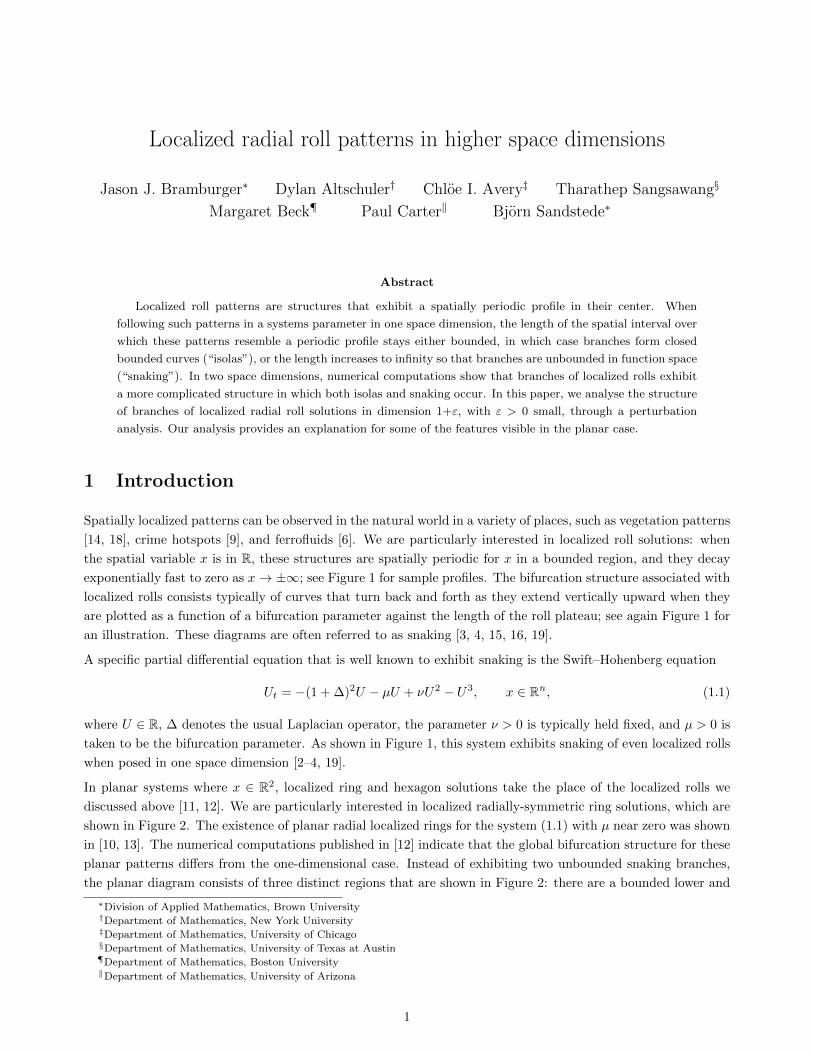
Localized radial roll patterns in higher space dimensions

Jason J. Bramburger∗ Dylan Altschuler† Chloe I. Avery‡ Tharathep Sangsawang§

Margaret Beck¶ Paul Carter‖ Bjorn Sandstede∗

Abstract

Localized roll patterns are structures that exhibit a spatially periodic profile in their center. When

following such patterns in a systems parameter in one space dimension, the length of the spatial interval over

which these patterns resemble a periodic profile stays either bounded, in which case branches form closed

bounded curves (“isolas”), or the length increases to infinity so that branches are unbounded in function space

(“snaking”). In two space dimensions, numerical computations show that branches of localized rolls exhibit

a more complicated structure in which both isolas and snaking occur. In this paper, we analyse the structure

of branches of localized radial roll solutions in dimension 1+ε, with ε > 0 small, through a perturbation

analysis. Our analysis provides an explanation for some of the features visible in the planar case.

1 Introduction

Spatially localized patterns can be observed in the natural world in a variety of places, such as vegetation patterns

[14, 18], crime hotspots [9], and ferrofluids [6]. We are particularly interested in localized roll solutions: when

the spatial variable x is in R, these structures are spatially periodic for x in a bounded region, and they decay

exponentially fast to zero as x→ ±∞; see Figure 1 for sample profiles. The bifurcation structure associated with

localized rolls consists typically of curves that turn back and forth as they extend vertically upward when they

are plotted as a function of a bifurcation parameter against the length of the roll plateau; see again Figure 1 for

an illustration. These diagrams are often referred to as snaking [3, 4, 15, 16, 19].

A specific partial differential equation that is well known to exhibit snaking is the Swift–Hohenberg equation

Ut = −(1 + ∆)2U − µU + νU2 − U3, x ∈ Rn, (1.1)

where U ∈ R, ∆ denotes the usual Laplacian operator, the parameter ν > 0 is typically held fixed, and µ > 0 is

taken to be the bifurcation parameter. As shown in Figure 1, this system exhibits snaking of even localized rolls

when posed in one space dimension [2–4, 19].

In planar systems where x ∈ R2, localized ring and hexagon solutions take the place of the localized rolls we

discussed above [11, 12]. We are particularly interested in localized radially-symmetric ring solutions, which are

shown in Figure 2. The existence of planar radial localized rings for the system (1.1) with µ near zero was shown

in [10, 13]. The numerical computations published in [12] indicate that the global bifurcation structure for these

planar patterns differs from the one-dimensional case. Instead of exhibiting two unbounded snaking branches,

the planar diagram consists of three distinct regions that are shown in Figure 2: there are a bounded lower and

∗Division of Applied Mathematics, Brown University†Department of Mathematics, New York University‡Department of Mathematics, University of Chicago§Department of Mathematics, University of Texas at Austin¶Department of Mathematics, Boston University‖Department of Mathematics, University of Arizona

1

0.18 0.185 0.19 0.195 0.2 0.205 0.21 0.215110

120

130

140

150

160

170

0 50 100 150-0.6

-0.4

-0.2

0

0.2

0.4

0.6

0.8

1

1.2

0 50 100 150-0.6

-0.4

-0.2

0

0.2

0.4

0.6

0.8

1

1.2

Figure 1: The bifurcation diagram of localized rolls to equation (1.1) in dimension n = 1 for ν = 1.6. Two

branches of solutions move back and forth in µ whilst the L2-norm of the associated localized solutions increases.

Sample profiles are given on the right for each of the branches, where we restrict the domain to x ≥ 0 and note

that the full solutions on R are symmetric over x = 0. Solutions are obtained at the parameter values µ = 0.2105

(top) and µ = 0.2110 (bottom). Notice that the profiles along one branch have a maximum at x = 0, while the

profiles along the other branch have a minimum at x = 0.

an unbounded upper snaking branch, which are separated by a region of stacked isolas. Furthermore, the upper

snaking branch seems to collapse onto a vertical line located approximately at µ = 0.204. The spatial profiles

retain the same basic shape through these different regions. However, along the lower branch, rolls are added in

the far field, while rolls are added near the center of the pattern along the upper snaking branch.

The goal of this paper is to shed light on the differences between the bifurcation diagrams in one and two space

dimensions. To illustrate the scope of our paper, we first outline how radial solutions can be found for the

Swift–Hohenberg equation. Writing U(x) = U(r) with r := |x|, we see that radially-symmetric steady-states of

the Swift–Hohenberg equation (1.1) satisfy the ordinary differential equation (ODE)

0 = −(

1 +n− 1

r∂r + ∂rr

)2

U − µU + νU2 − U3, r > 0. (1.2)

Note that the space dimension n enters explicitly into the second term on the right-hand side. As suggested in

[12], we will carry out a perturbation analysis near n = 1 by setting n = 1 + ε with 0 < ε � 1. While there is

no meaningful connection between n and the underlying dimension unless n is an integer, we can study (1.2) in

its own right for real n. Rewriting (1.2) as a first-order system, we obtain the nonautonomous ODE

u′1 = u2,

u′2 = u3 − u1 −ε

ru2,

u′3 = u4,

u′4 = −u3 − µu1 + νu21 − u3

1 −ε

ru4,

(1.3)

where ′ = ddr ,

u1 = U, u2 = ∂rU, u3 = (1 +ε

r∂r + ∂rr)U, u4 = ∂r(1 +

ε

r∂r + ∂rr)U,

and 0 ≤ ε � 1 is now a small parameter that connects the one-dimensional system (ε = 0, corresponding to

n = 1) to the 1 + ε-dimensional system. Since the one-dimensional case is well understood, we can leverage the

2

0.175 0.18 0.185 0.19 0.195 0.2 0.205 0.21100

200

300

400

500

600

700

800

900

Isol

as

Low

erB

ranc

h

Upp

er B

ranc

h

Figure 2: Snaking in the planar Swift–Hohenberg equation with ν = 1.6. The bifurcation diagram is composed

of three distinct regions: the lower snaking branch (magenta), stacked isolas (turquoise), and the upper snaking

branch (brown). The isolas are a collection of closed curves, as is demonstrated in the upper right inset. The

bottom right inset provides a contour plot of the bifurcating localized spot solutions of the Swift–Hohenberg equa-

tion.

existing theoretical approaches to understand what structural changes the nonautonomous perturbation term

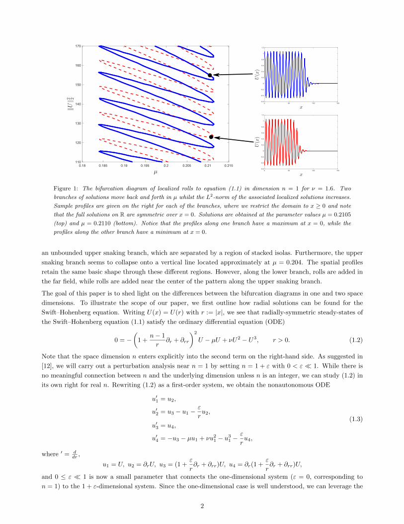
induces as ε changes near zero. Figure 3 illustrates the connection between even localized roll patterns of (1.1)

and heteroclinic solutions that connect periodic solutions to the equilibrium u = 0 of the ODE (1.3) in the

one-dimensional situation.

When ε = 0, equation (1.3) is autonomous, reversible under r 7→ −r, and conservative. Reversibility and the

existence of a conserved quantity H : R4 → R allows us to assume that (1.3) admits a cylinder of reversible

periodic orbits that is parametrized by the phase of the periodic patterns along its circumference and the value

U(r)

u(r)

Figure 3: The left panel illustrates an even localized roll solution U(r) of the Swift–Hohenberg equation (1.2). The

right panel shows the same profile now viewed as a solution u(r) of the first-order dynamical system (1.3): the

associated trajectory of (1.3) starts sufficiently close to the periodic orbit γ, follows this orbit for some amount

of time r, and converges to the trivial equilibrium u = 0 along its stable manifold.

3

<latexit sha1_base64="jBwNY3dzluIKK7a26JGabkJUQyc=">AAACE3icdZDNTsJAFIWn/iL+oS7dNLKBBElLgg07Ek1w4QKjBRJBMjNccGQ6bTpTUkJ8B1cm+iyujFsfwEdxZ4slsSae1c13z5zcOcTjTCrD+NSWlldW19YzG9nNre2d3dzefku6gU/Bpi53/Q7BEjgTYCumOHQ8H7BDOLTJ+DTetyfgS+aKazX1oOfgkWBDRrGKUKt9KwtGsZ/LG2XLtKwTUzfKxlzxYFYrZk03E5JHiZr93Fd34NLAAaEox1LemIanejPsK0Y5PGS7gQQP0zEewWx+YxphR8qpQ9LQwepOekDTNAwEo+7gT2bIVah8HEEJysFMDF2hZg3GuX6FhVzwKDBeFM7YiClZuoj+LEoNH2BcTJl/JXOsIGTqGBPiw4TNW4otxOWDODAbdbUoRP9/sCvlWtm8NPL1alJaBh2iI1RAJrJQHZ2jJrIRRffoET2jF+1Je9XetPcf65KWvDlAKWkf3/pVn/0=</latexit>

Plane of Neumann Boundary

Conditions

H(u)

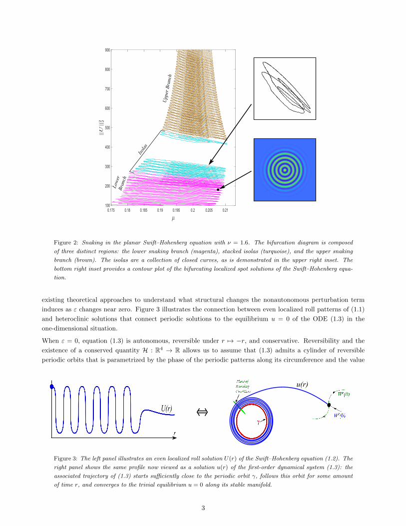
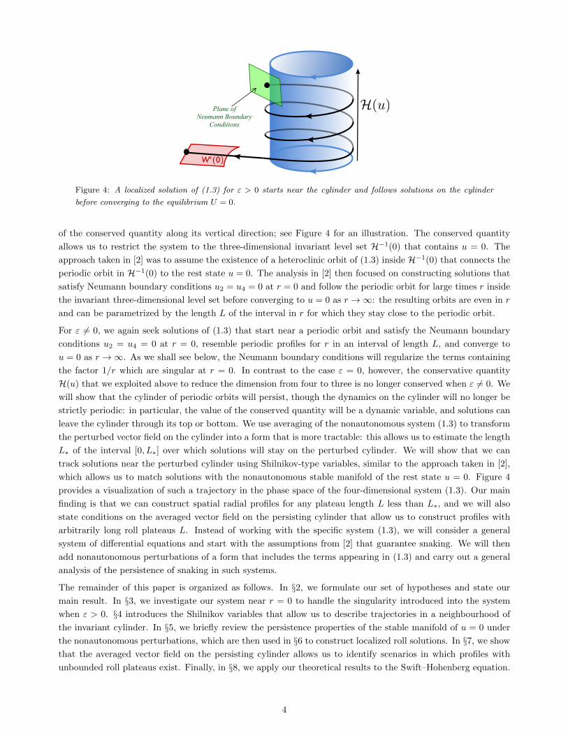
Figure 4: A localized solution of (1.3) for ε > 0 starts near the cylinder and follows solutions on the cylinder

before converging to the equilibrium U = 0.

of the conserved quantity along its vertical direction; see Figure 4 for an illustration. The conserved quantity

allows us to restrict the system to the three-dimensional invariant level set H−1(0) that contains u = 0. The

approach taken in [2] was to assume the existence of a heteroclinic orbit of (1.3) inside H−1(0) that connects the

periodic orbit in H−1(0) to the rest state u = 0. The analysis in [2] then focused on constructing solutions that

satisfy Neumann boundary conditions u2 = u4 = 0 at r = 0 and follow the periodic orbit for large times r inside

the invariant three-dimensional level set before converging to u = 0 as r →∞: the resulting orbits are even in r

and can be parametrized by the length L of the interval in r for which they stay close to the periodic orbit.

For ε 6= 0, we again seek solutions of (1.3) that start near a periodic orbit and satisfy the Neumann boundary

conditions u2 = u4 = 0 at r = 0, resemble periodic profiles for r in an interval of length L, and converge to

u = 0 as r →∞. As we shall see below, the Neumann boundary conditions will regularize the terms containing

the factor 1/r which are singular at r = 0. In contrast to the case ε = 0, however, the conservative quantity

H(u) that we exploited above to reduce the dimension from four to three is no longer conserved when ε 6= 0. We

will show that the cylinder of periodic orbits will persist, though the dynamics on the cylinder will no longer be

strictly periodic: in particular, the value of the conserved quantity will be a dynamic variable, and solutions can

leave the cylinder through its top or bottom. We use averaging of the nonautonomous system (1.3) to transform

the perturbed vector field on the cylinder into a form that is more tractable: this allows us to estimate the length

L∗ of the interval [0, L∗] over which solutions will stay on the perturbed cylinder. We will show that we can

track solutions near the perturbed cylinder using Shilnikov-type variables, similar to the approach taken in [2],

which allows us to match solutions with the nonautonomous stable manifold of the rest state u = 0. Figure 4

provides a visualization of such a trajectory in the phase space of the four-dimensional system (1.3). Our main

finding is that we can construct spatial radial profiles for any plateau length L less than L∗, and we will also

state conditions on the averaged vector field on the persisting cylinder that allow us to construct profiles with

arbitrarily long roll plateaus L. Instead of working with the specific system (1.3), we will consider a general

system of differential equations and start with the assumptions from [2] that guarantee snaking. We will then

add nonautonomous perturbations of a form that includes the terms appearing in (1.3) and carry out a general

analysis of the persistence of snaking in such systems.

The remainder of this paper is organized as follows. In §2, we formulate our set of hypotheses and state our

main result. In §3, we investigate our system near r = 0 to handle the singularity introduced into the system

when ε > 0. §4 introduces the Shilnikov variables that allow us to describe trajectories in a neighbourhood of

the invariant cylinder. In §5, we briefly review the persistence properties of the stable manifold of u = 0 under

the nonautonomous perturbations, which are then used in §6 to construct localized roll solutions. In §7, we show

that the averaged vector field on the persisting cylinder allows us to identify scenarios in which profiles with

unbounded roll plateaus exist. Finally, in §8, we apply our theoretical results to the Swift–Hohenberg equation.

4

2 Main results

Consider the ordinary differential equation

ux = f(u, µ), (2.1)

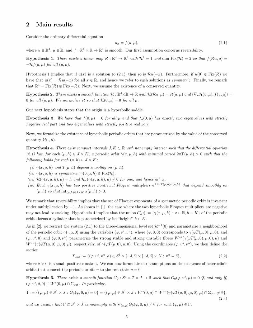
where u ∈ R4, µ ∈ R, and f : R4 × R→ R4 is smooth. Our first assumption concerns reversibility.

Hypothesis 1. There exists a linear map R : R4 → R4 with R2 = 1 and dim Fix(R) = 2 so that f(Ru, µ) =

−Rf(u, µ) for all (u, µ).

Hypothesis 1 implies that if u(x) is a solution to (2.1), then so is Ru(−x). Furthermore, if u(0) ∈ Fix(R) we

have that u(x) = Ru(−x) for all x ∈ R, and hence we refer to such solutions as symmetric. Finally, we remark

that R4 = Fix(R)⊕ Fix(−R). Next, we assume the existence of a conserved quantity.

Hypothesis 2. There exists a smooth function H : R4×R→ R with H(Ru, µ) = H(u, µ) and 〈∇uH(u, µ), f(u, µ)〉 =

0 for all (u, µ). We normalize H so that H(0, µ) = 0 for all µ.

Our next hypothesis states that the origin is a hyperbolic saddle.

Hypothesis 3. We have that f(0, µ) = 0 for all µ and that fu(0, µ) has exactly two eigenvalues with strictly

negative real part and two eigenvalues with strictly positive real part.

Next, we formalize the existence of hyperbolic periodic orbits that are parametrized by the value of the conserved

quantity H(·, µ).

Hypothesis 4. There exist compact intervals J,K ⊂ R with nonempty interior such that the differential equation

(2.1) has, for each (µ, h) ∈ J ×K, a periodic orbit γ(x, µ, h) with minimal period 2πT (µ, h) > 0 such that the

following holds for each (µ, h) ∈ J ×K:

(i) γ(x, µ, h) and T (µ, h) depend smoothly on (µ, h).

(ii) γ(x, µ, h) is symmetric: γ(0, µ, h) ∈ Fix(R).

(iii) H(γ(x, µ, h), µ) = h and Hu(γ(x, µ, h), µ) 6= 0 for one, and hence all, x.

(iv) Each γ(x, µ, h) has two positive nontrivial Floquet multipliers e±2πT (µ,h)α(µ,h) that depend smoothly on

(µ, h) so that inf(µ,h)∈J×K α(µ, h) > 0.

We remark that reversibility implies that the set of Floquet exponents of a symmetric periodic orbit is invariant

under multiplication by −1. As shown in [1], the case where the two hyperbolic Floquet multipliers are negative

may not lead to snaking. Hypothesis 4 implies that the union C(µ) := {γ(x, µ, h) : x ∈ R, h ∈ K} of the periodic

orbits forms a cylinder that is parametrized by its “height” h ∈ K.

As in [2], we restrict the system (2.1) to the three-dimensional level set H−1(0) and parametrize a neighborhood

of the periodic orbit γ(·, µ, 0) using the variables (ϕ, vs, vu), where (ϕ, 0, 0) corresponds to γ(ϕT (µ, 0), µ, 0), and

(ϕ, vs, 0) and (ϕ, 0, vu) parametrize the strong stable and strong unstable fibers W ss(γ(ϕT (µ, 0), µ, 0), µ) and

Wuu(γ(ϕT (µ, 0), µ, 0), µ), respectively, of γ(ϕT (µ, 0), µ, 0). Using the coordinates (ϕ, vs, vu), we then define the

section

Σout := {(ϕ, vs, vu, h) ∈ S1 × [−δ, δ]× [−δ, δ]×K : vu = δ}, (2.2)

where δ > 0 is a small positive constant. We can now formulate our assumptions on the existence of heteroclinic

orbits that connect the periodic orbits γ to the rest state u = 0.

Hypothesis 5. There exists a smooth function G0 : S1 × I × J → R such that G0(ϕ, vs, µ) = 0 if, and only if,

(ϕ, vs, δ, 0) ∈W s(0, µ) ∩ Σout. In particular,

Γ := {(ϕ, µ) ∈ S1 × J : G0(ϕ, 0, µ) = 0} = {(ϕ, µ) ∈ S1 × J : W s(0, µ) ∩Wuu(γ(ϕT (µ, 0), µ, 0), µ) ∩ Σout 6= ∅},(2.3)

and we assume that Γ ⊂ S1 × J is nonempty with ∇(ϕ,µ)G0(ϕ, 0, µ) 6= 0 for each (ϕ, µ) ∈ Γ.

5

m

j

0

2p

m

m

j

0

2p

m

m

j

0

2p

m

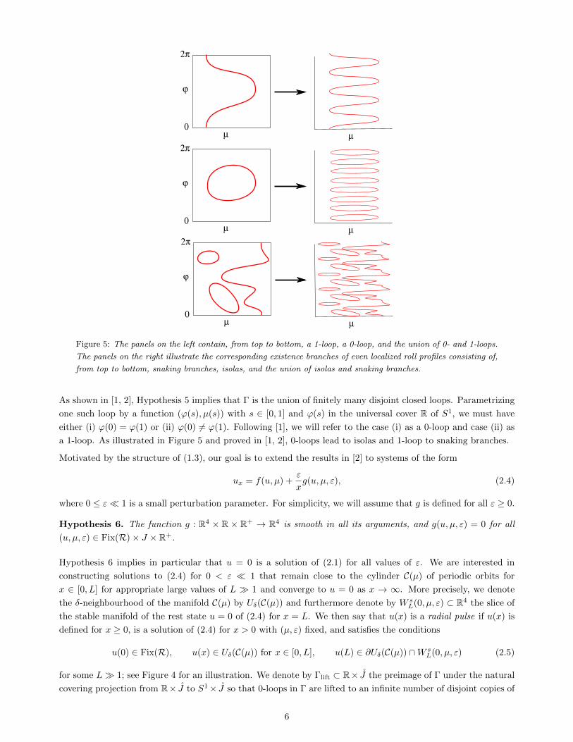
Figure 5: The panels on the left contain, from top to bottom, a 1-loop, a 0-loop, and the union of 0- and 1-loops.

The panels on the right illustrate the corresponding existence branches of even localized roll profiles consisting of,

from top to bottom, snaking branches, isolas, and the union of isolas and snaking branches.

As shown in [1, 2], Hypothesis 5 implies that Γ is the union of finitely many disjoint closed loops. Parametrizing

one such loop by a function (ϕ(s), µ(s)) with s ∈ [0, 1] and ϕ(s) in the universal cover R of S1, we must have

either (i) ϕ(0) = ϕ(1) or (ii) ϕ(0) 6= ϕ(1). Following [1], we will refer to the case (i) as a 0-loop and case (ii) as

a 1-loop. As illustrated in Figure 5 and proved in [1, 2], 0-loops lead to isolas and 1-loop to snaking branches.

Motivated by the structure of (1.3), our goal is to extend the results in [2] to systems of the form

ux = f(u, µ) +ε

xg(u, µ, ε), (2.4)

where 0 ≤ ε� 1 is a small perturbation parameter. For simplicity, we will assume that g is defined for all ε ≥ 0.

Hypothesis 6. The function g : R4 × R × R+ → R4 is smooth in all its arguments, and g(u, µ, ε) = 0 for all

(u, µ, ε) ∈ Fix(R)× J × R+.

Hypothesis 6 implies in particular that u = 0 is a solution of (2.1) for all values of ε. We are interested in

constructing solutions to (2.4) for 0 < ε � 1 that remain close to the cylinder C(µ) of periodic orbits for

x ∈ [0, L] for appropriate large values of L � 1 and converge to u = 0 as x → ∞. More precisely, we denote

the δ-neighbourhood of the manifold C(µ) by Uδ(C(µ)) and furthermore denote by W sL(0, µ, ε) ⊂ R4 the slice of

the stable manifold of the rest state u = 0 of (2.4) for x = L. We then say that u(x) is a radial pulse if u(x) is

defined for x ≥ 0, is a solution of (2.4) for x > 0 with (µ, ε) fixed, and satisfies the conditions

u(0) ∈ Fix(R), u(x) ∈ Uδ(C(µ)) for x ∈ [0, L], u(L) ∈ ∂Uδ(C(µ)) ∩W sL(0, µ, ε) (2.5)

for some L� 1; see Figure 4 for an illustration. We denote by Γlift ⊂ R× J the preimage of Γ under the natural

covering projection from R× J to S1× J so that 0-loops in Γ are lifted to an infinite number of disjoint copies of

6

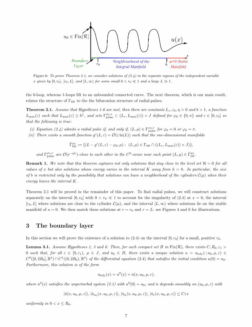
Figure 6: To prove Theorem 2.1, we consider solutions of (2.4) in the separate regions of the independent variable

x given by [0, r0], [r0, L], and [L,∞) for some small 0 < r0 � 1 and a large L� 1.

the 0-loop, whereas 1-loops lift to an unbounded connected curve. The next theorem, which is our main result,

relates the structure of Γlift to the the bifurcation structure of radial-pulses.

Theorem 2.1. Assume that Hypotheses 1-6 are met, then there are constants L∗, ε0, η > 0 and b > 1, a function

Lmax(ε) such that Lmax(ε) ≥ b1ε , and sets Γϕ0,ε

pulse ⊂ (L∗, Lmax(ε)) × J defined for ϕ0 ∈ {0, π} and ε ∈ [0, ε0] so

that the following is true:

(i) Equation (2.4) admits a radial pulse if, and only if, (L, µ) ∈ Γϕ0,εpulse for ϕ0 = 0 or ϕ0 = π.

(ii) There exists a smooth function gc(L, ε) = O(ε ln(L)) such that the one-dimensional manifolds

Γϕ0

lift := {(L− gc(L, ε)− ϕ0, µ) : (L, µ) ∈ Γlift ∩ ((L∗, Lmax(ε))× J)},

and Γϕ0,εpulse are O(e−ηL)-close to each other in the C0-sense near each point (L, µ) ∈ Γϕ0

lift.

Remark 1. We note that this theorem captures not only solutions that stay close to the level set H = 0 for all

values of x but also solutions whose energy varies in the interval K away from h = 0. In particular, the size

of b is restricted only by the possibility that solutions can leave a neighborhood of the cylinders C(µ) when their

energy leaves the interval K.

Theorem 2.1 will be proved in the remainder of this paper. To find radial pulses, we will construct solutions

separately on the interval [0, r0] with 0 < r0 � 1 to account for the singularity of (2.4) at x = 0, the interval

[r0, L] where solutions are close to the cylinder C(µ), and the interval [L,∞) where solutions lie on the stable

manifold of u = 0. We then match these solutions at r = r0 and r = L: see Figures 4 and 6 for illustrations.

3 The boundary layer

In this section we will prove the existence of a solution to (2.4) on the interval [0, r0] for a small, positive r0.

Lemma 3.1. Assume Hypotheses 1, 3 and 6. Then, for each compact set B in Fix(R), there exists C,R0, ε1 >

0 such that, for all ε ∈ [0, ε1), µ ∈ J , and u0 ∈ B, there exists a unique solution u = ubdy(·;u0, µ, ε) ∈C0([0, 2R0],R4) ∩C1((0, 2R0),R4) of the differential equation (2.4) that satisfies the initial condition u(0) = u0.

Furthermore, this solution is of the form

ubdy(x) = u0(x) + u(x, u0, µ, ε),

where u0(x) satisfies the unperturbed system (2.1) with u0(0) = u0, and u depends smoothly on (u0, µ, ε) with

|u(x, u0, µ, ε)|, |uu0(x, u0, µ, ε)|, |uµ(x, u0, µ, ε)|, |uε(x, u0, µ, ε)| ≤ Cεx

uniformly in 0 < x ≤ R0.

7

Proof. Let u0(x) be the solution of ux = f(u, µ) with u0(0) = u0 ∈ Fix(R). Writing u(x) = u0(x) + v(x), we see

that u(x) is a solution to (2.4) of the form desired by the lemma if, and only if, v(x) satisfies the nonautonomous

initial-value problem

vx = f(u0(x) + v, µ)− f(u0(x), µ) +ε

xg(u0(x) + v, µ, ε), v(0) = 0. (3.1)

We can write u0(x) = u0 + xu(x) and

f(u0(x) + v, µ)− f(u0(x), µ) = f(x, v, µ)v.

Furthermore, denoting by PR the projection onto Fix(−R) along Fix(R), we can use Hypothesis 6 to write

1

xg(u, µ, ε) =

1

xg(u, µ, ε)PRu.

Using the Banach space

X =

{v ∈ C0([0, 2R0],R4) : v(0) = 0 and ‖v‖ := sup

x∈[0,R0]

|v(x)|x

<∞},

we then define, for v ∈ X, the new function

[Tv](x) :=

∫ x

0

[f(u0(s) + v(s))− f(u0(s), µ) +

ε

sg(u0(s) + v(s), µ, ε)

]ds

=

∫ x

0

[f(s, v(s), µ)v(s) +

ε

sg(u0(s) + v(s), µ, ε)PR(u0 + su(s) + v(s))

]ds

=:

∫ x

0

[f(s, v(s), µ)v(s) + εg1(s, v(s), µ, ε) +

ε

sg2(s, v(s), µ, ε)v(s)

]ds

where we used that PRu0 = 0. Since fixed points of T are in one-to-one correspondence with solutions of (3.1),

it suffices to show that, for sufficiently small R0, δ > 0, T maps the ball of radius δ centered at the origin in

X into itself and is a uniform contraction on this ball: these properties are straightforward to verify using the

uniform bounds on the smooth functions f and g1,2 and their Lipschitz constants in v. We omit the details.

4 Shilnikov variables

The results of the preceding section allow us to restrict the analysis of (2.4) to the region x ≥ r0 for each fixed,

but arbitrary, value of r0. For each such fixed r0, we will construct a local coordinate system akin to Shilnikov

variables for the nonautonomous system (2.4) near the cylinder C(µ) of periodic orbits.

Choose a closed nonempty interval K0 ⊂ K. For each δ > 0, we define I := [−δ, δ] and let V := R× I × I ×K,

V0 := R× I × I ×K0, and C0(µ) := {γ(x, µ, h) : x ∈ R, h ∈ K0}.

Lemma 4.1. Assume that Hypotheses 1-6 are met, then there is a δ > 0 such that the following is true for each

fixed r0 ∈ (0, R0]: there is an ε2 > 0 such that there are smooth real-valued functions (hc1,2,3, hs, hu, he1,2,3) and a

smooth change of coordinates that puts (2.4) restricted to a uniform neighborhood of C0(µ) into the form

vcx = 1 +ε

xhc1(vc, vh, µ, ε) +

ε2

x2hc2(x, vc, vh, µ, ε) +

ε

xhc3(x, v, µ, ε)vsvu

vsx = −[α(µ, vh) + hs(x, v, µ, ε)]vs

vsu = [α(µ, vh) + hu(x, v, µ, ε)]vu

vhx =ε

xhe1(vc, vh, µ, ε) +

ε2

x2he2(x, vc, vh, µ, ε) +

ε

xhe3(x, v, µ, ε)vsvu,

(4.1)

8

where (x, µ, ε) ∈ [r0,∞) × J × [0, ε2] and v = (vc, vs, vu, vh) ∈ V. The functions (hc1,2,3, hs, hu, he1,2,3) are

2πT (µ, vh)-periodic in vc, uniformly bounded for x ≥ r0, and globally Lipschitz in v ∈ V. Moreover, hs and hu

vanish identically when (vs, vu, ε) = (0, 0, 0), and he1,2 vanish identically for vh ∈ ∂K. The reverser R acts via

R(vc, vs, vu, vh) = (−vc, vu, vs, vh).

Proof. Let vh := H(u, µ), then, for each solution u(x) of (2.4), we have

vhx = ∇uH(u, µ) · ux = ∇uH(u, µ) ·(f(u, µ) +

ε

xg(u, µ, ε)

)=ε

x∇uH(u, µ) · g(u, µ, ε) (4.2)

upon using Hypothesis 2. Note that the identity H(Ru, µ) = H(u, µ) implies that vh remains unchanged under

the action ofR. As in [2, 5], we can now use Hypothesis 4(iv) to introduce the invertible coordinate transformation

u = Q(v, µ) defined for v = (vc, vs, vu, vh) ∈ R × I × I ×K so that, for ε = 0, Q(vc, 0, 0, vh, µ) = γ(vc, µ, vh)

parametrizes the periodic orbits, the sets {vu = 0} and {vs = 0} parametrize, respectively, the strong stable and

strong unstable fibers of γ(vc, µ, vh), and {vh = h} gives H−1(h). Note that the action of the reverser follows

from Hypothesis 4(ii). Referring again to [2, 5], the vector field in the new coordinates v is then given by

vcx = 1 + f c(v, µ)vsvu +ε

xf c(x, v, µ, ε)

vsx = −[α(µ, vh) + fs1 (v, µ)vs + fs2 (v, µ)vu]vs +ε

xfs(x, v, µ, ε)

vsu = [α(µ, vh) + fu1 (v, µ)vs + fu2 (v, µ)vu]vu +ε

xfu(x, v, µ, ε)

vhx =ε

xfh(x, v, µ, ε)

(4.3)

for each µ ∈ J and ε ≥ 0, where the functions f j with j = c, s, u, h represent the terms coming from the

perturbation g(Q(v), µ, ε), with fh given by (4.2).

Note that the set {vs = vu = 0}, which corresponds to the cylinder C(µ) in the original variables, forms an

invariant, normally hyperbolic manifold for (4.3) when ε = 0. We claim that this invariant manifold persists

as an integral manifold for (4.3) for all sufficiently small ε > 0. Indeed, it is straightforward to check that our

system satisfies the hypotheses stated in [7, Theorem 2.2], and this theorem then guarantees the existence of a

smooth function Θ(x, vc, vh, µ, ε) that is defined for all 0 < ε� 1 such that{(vs, vu) =

ε

xΘ(x, vc, vh, µ, ε); (vc, vh) ∈ R× I

}is a smooth integral manifold for (4.3). Furthermore, the transformation Θ is 2πT (µ, vh)-periodic in vc, uniformly

bounded in x ≥ r0, and does not depend on the choice of r0. Defining the new variables

(vs, vu) := (vs, vu)− ε

xΘ(x, vc, vh, µ, ε)

and noting that {(vs, vu) = 0} corresponds to the integral manifold we just constructed, we see that, upon

dropping the tildes, the system (4.3) becomes

vcx = 1 +ε

xHc

1(vc, vh, µ, ε) +ε2

x2Hc

2(x, vc, vh, µ, ε) +Hc3(x, v, µ, ε)vs +Hc

4(x, v, µ, ε)vu

vsx = −[α(µ, vh) +Hs1(x, v, µ, ε)]vs +Hs

2(x, v, µ, ε)vu

vsu = [α(µ, vh) +Hu1 (x, v, µ, ε)]vu +Hu

2 (x, v, µ, ε)vs

vhx =ε

xHh

1 (vc, vh, µ, ε) +ε2

x2Hh

2 (x, vc, vh, µ, ε) +ε

xHh

3 (x, v, µ, ε)vs +ε

xHh

4 (x, v, µ, ε)vu,

(4.4)

where Hc,h1 (vc, vh, µ, ε) = f c,h(vc, 0, 0, vh, µ, ε). The functions appearing in (4.4) are 2πT (µ, vh)-periodic in vc,

uniformly bounded in their arguments, independent of r0 for x ≥ r0, and globally Lipschitz in v. Furthermore,

Hs,uj vanish when (vs, vu, ε) = (0, 0, 0) for j = 1, 2. By locally straightening the stable and unstable fibers of

9

the integral manifold so that they correspond, respectively, to vu = 0 and vs = 0, we can bring (4.4) into the

normal form (4.1); see [5] or [8, Chapter 4] for details. Finally, we can multiply the functions he1,2 by appropriate

cutoff functions so that the products coincide with the original functions for vh ∈ K0 and vanish identically when

vh ∈ ∂K. Throughout these transformations, the action of the reverser remains as stated in the lemma.

Note that Lemma 4.1 shows that {(vs, vu) = 0} is an integral manifold of (2.4) that corresponds to the perturbed

invariant cylinder C(µ) of periodic orbits of (2.1). The vector field on this integral manifold is given by(vc

vh

)x

=

(1

0

)+ε

xh1(vc, vh, µ, ε) +

ε2

x2h2(x, vc, vh, µ, ε) =:

(1

0

)+ε

xF c(x, vc, vh, µ, ε). (4.5)

Due to the fact that when ε > 0 the flow of (2.4) can move between the level sets of the conserved quantity H,

there is the possibility that trajectories can leave V by having vh /∈ K, representing a trajectory that flows off

the top or bottom of the integral manifold. To prevent this from happening we have applied cutoff functions to

guarantee that V is invariant, but we note that the system (4.1) does not completely correspond to the original

perturbed differential equation (2.4). This leads to the following lemma which precisely determines when a

trajectory of (4.5) corresponds to a trajectory of (2.4), along with some important properties about solutions on

the integral manifold.

Lemma 4.2. For each fixed r0 ∈ (0, 1] and given L ≥ 1/r0, ϕ1 ∈ R, and h1 ∈ K, there exists a unique solution

Φ(x; r0, L, ϕ1, h1, µ, ε) to (4.5) that satisfies the boundary conditions

vc(L) = ϕ1, vh(L) = h1 (4.6)

and lies in I ×K for x ∈ [r0, L]. This solution is smooth in (x, r0, L, ϕ1, h1, µ, ε) and we have

vc(r0) = ϕ1 − L+ r0 + gc(L, µ, ε), (4.7)

with |gc(L, µ, ε)|, |vhϕ(r0)|, |vhh1(r0)|, |vhµ(r0)| ≤ Cgε ln(L), for some constant Cg > 0. This solution provides a

genuine solution of the original system whenever Φh(x; r0, L, ϕ1, h1, µ, ε) ∈ K0 for x ∈ [r0, L].

Proof. Since I × ∂K is invariant under (4.5) for all ε > 0, existence, uniqueness, and smoothness of the solution

is immediate. Therefore, it remains to estimate vc(r0). We write vc(x) = ϕ1 +x−L+ vc(x) so that the boundary

condition vc(L) = ϕ1 is equivalent to vc(L) = 0. Thus, vc(r0) is given implicitly by

vc(r0) = ε

∫ r0

L

hc1(vc(s), vh(s), µ, ε)

sds+ ε2

∫ r0

L

hc2(s, vc(s), vh(s), µ, ε)

s2ds.

Bounding hc1,2 by a uniform constant C1 > 0, we obtain

|vc(r0)| = |gc(L, µ, ε)| ≤ εC1(ln(L) + | ln(r0)|) ≤ εCg ln(L)

with Cg := C1(1 + | ln(r0)|/ ln(L)) ≤ 2C1 for L ≥ 1/r0. The bounds on |vh(r0)| and its derivatives are handled

in an identical manner.

Proposition 4.3. There exist η, L0,M > 0 such that, for each fixed 0 < r0 ≤ 1, there exists an ε3 > 0 such that

the following holds: pick 0 ≤ ε ≤ ε3, L ≥ L0, and let Φ(x; r0, L, ϕ1, h1, µ, ε) be as above, then, for each as ∈ I,

there exists a unique solution v(x) = v(x; r0, L, as, ϕ1, h1, µ, ε) ∈ V to (4.1) defined for x ∈ [r0, L] so that

vc(L) = ϕ1, vs(r0) = as, vu(L) = δ, vh(L) = h1.

Furthermore, this solution satisfies

|vs(x)| ≤Me−ηx, |vu(x)| ≤Meη(x−L), |(vc(x), vh(x))T − Φ(x; r0, L, ϕ1, h1, µ, ε)| ≤Me−ηL (4.8)

for all x ∈ [r0, L], v(x) is smooth in (x, r0, L, as, ϕ1, h1, µ, ε), and the bounds (4.8) also hold for these derivatives.

10

Proof. We will show that the assumptions of [17, Theorem 2.2] are satisfied: our statements then follow directly

from this theorem. Note that restricting to x ≥ r0 and choosing 0 ≤ ε2 ≤ r20 guarantees that the right-hand

side of (4.1) is bounded uniformly in x. It remains to establish appropriate exponential bounds for solutions of

the linearized dynamics of (4.1). Linearizing (4.1) along the solution (vc, vs, vu, vh) = (Φc(x), 0, 0,Φh(x)), where

(Φc(x),Φh(x))T = Φ(x; r0, L, µ, ε) satisfies (4.5)–(4.6) on [r0, L], we arrive at the linear system

vsx = −[α(Φh(x)) + hs(x,Φc(x), 0, 0,Φh(x), ε)]vs (4.9a)

vux = [α(Φh(x)) + hu(x,Φc(x), 0, 0,Φh(x), ε)]vu (4.9b)

wx =ε

xD(vc,vh)F

c(x,Φc(x),Φh(x), ε)c, (4.9c)

where w = (vc, vh)T ; note that we have suppressed the dependence on µ ∈ J for notational convenience.

Lemma 4.1 implies that (hs, hu) vanish uniformly when ε = 0, and Hypothesis 4 implies that α(µ, vh) is bounded

away from zero uniformly in (µ, vh) ∈ J ×K. Hence, for ε > 0 taken sufficiently small, the right-hand sides of

(4.9a) and (4.9b) are uniformly bounded away from zero,and we conclude that there are constants ηs, ηu > 0

and M0 > 0 such that the solution operators Ψs(x, s),Ψu(x, s) of (4.9a) and (4.9b), respectively, satisfy

|Ψs(x, y)| ≤M0e−ηs(x−y) and |Ψu(y, x)| ≤M0eη

u(y−x)

for r0 ≤ y ≤ x ≤ L and ε > 0 sufficiently small. Furthermore, we may take ηu > 0 so that −ηs + ηu < 0.

We now turn to (4.9c). Lemma 4.1 guarantees that there is a constant C > 0 with |D(vc,vh)Fc(x,Φc(x),Φh(x), ε)| ≤

C uniformly in all arguments, and we conclude that

|wx| ≤εC

x|w| ≤ ε 1

2C|w|

provided we pick 0 ≤ ε2 ≤ r20. Denoting the solution operator to (4.9c) by Ψc(x, y), we have

|Ψc(x, y)| ≤ e√εC(x−y)

for all x, y ∈ [r0, L], independently of r0 and L, which verifies [17, Hypothesis (E1) in Theorem 2.2]. Finally,

taking ε > 0 and sufficiently small, we can guaranteed that

ηs + ηu +√εK2 < 0 < ηu −√εC,

which verifies [17, Hypothesis (D2) in Theorem 2.2]. We have now verified all hypotheses required to obtain the

result in the statement of Proposition 4.3.

Proposition 4.3 shows that we can understand the dynamics of (4.1) via solutions Φ(x; r0, L, ϕ1, h1, µ, ε) to (4.5).

In §7, we will explore conditions on the vector field on the integral manifold that imply that solutions to (4.5)–

(4.6) stay in K0 for all x, and therefore by Lemma 4.2 correspond to genuine solution to (2.4). Prior to doing so

though, we continue our exploration of the full augmented vector field (4.5) by obtaining radial pulse solutions

in this situation and work to understand their bifurcation characteristics.

5 The stable manifold

We now describe the set of solutions u(x) that converge to the trivial equilibrium as x → ∞. Recall that

Hypothesis 6 implies that u = 0 persists as an equilibrium of the nonautonomous system (2.4) for all ε ≥ 0.

Hence, for any L ≥ 1, we define the section of the stable manifold of the trivial solution at x = L to be

W sL(0, µ, ε) := {u0 ∈ R4 : u(x) satisfies (2.4) with u(L) = u0, and u(x)→ 0 as x→∞}.

11

Using the constant δ > 0 introduced in Lemma 4.1, we define the section Σout to be

Σout = R× I × {vu = δ} ×K.

First, we show that W sL(0, µ, ε) is a regular perturbation of W s(0, µ) in ε.

Lemma 5.1. For each L ≥ 1, the set W sL(0, µ, ε) is a two-dimensional manifold that is O(εL−1)-close in the

C1 sense to W s(0, µ), uniformly in µ.

Proof. The lemma follows from the uniform contraction mapping principle.

Next, we use the preceding lemma to provide a parametrization of the stable manifold in the Shilnikov variables.

Lemma 5.2. There exists ε4 > 0 and smooth real-valued functions zΓ, zh so that the following is true for each

ε ∈ [0, ε4] and L ≥ 1: we have that (ϕ, vs, δ, vh) with |vs|, |vh| < ε4 lies in W sL(0, µ, ε)∩Σout if, and only if, there

exists (ϕ∗, µ∗) ∈ Γ such that

ϕ = ϕ∗ + zΓ(L,ϕ∗, vs, µ∗, ε)∂G0

∂ϕ(ϕ∗, 0, µ∗)

µ = µ∗ + zΓ(L,ϕ∗, vs, µ∗, ε)∂G0

∂µ(ϕ∗, 0, µ∗)

vh = zh(L,ϕ∗, vs, µ∗, ε),

where the function G0 was defined in Hypothesis 5, and the functions zΓ and zh are bounded uniformly in L ≥ 1,

independent of L when ε = 0, and satisfy

zΓ(·, ϕ∗, 0, µ∗, 0) = 0, zh(·, ϕ∗, vs, µ∗, 0) = 0.

Proof. Define the subset of Σout × J ∼= R× I ×K × J given by

W sL(0, ε) :=

⋃µ∈J

(W sL(0, µ, ε) ∩ {vu = δ})× {µ}.

First, note that W sL(0, 0) is independent of L since (2.4) is autonomous when ε = 0. Hypothesis 5 implies that

Γ = W sL(0, 0) ∩ (R× {0} × {0} × J),

that the function G : R× I ×K × J → R2 given by

G(ϕ, vs, vh, µ) = (G0(ϕ, vs, µ), vh)

satisfies G−1(0) = W sL(0, 0), and that ∇(ϕ,vh,µ)G(ϕ, 0, 0, µ) ∈ R2×3 has full rank for all (ϕ, µ) ∈ Γ. Therefore, we

may use the columns of ∇(ϕ,vh,µ)G(ϕ, 0, 0, µ) to define normal vectors to Γ as a subset of W sL(0, ε) in the space

Σout×J to obtain the existence of the functions zΓ and zh, which represent deviations from Γ along these normal

vectors with respect to small perturbations in vs and ε. Smoothness properties and boundedness with respect to

L ≥ 1 follow from Lemma 5.1. The property zh(ϕ∗, vs, µ∗, 0) = 0 follows from the fact that W s(0, µ) ⊂ H−1(0)

for all µ ∈ J . This completes the proof.

6 Matching conditions

We can now match the solution segments we obtained in the preceding sections for 0 ≤ x ≤ r0, r0 ≤ x ≤ L,

and L ≥ x. Before doing so, we restate our definition (2.5) of radial pulses. We say that u(x) is a radial-pulse

12

solution to (2.4) if

u(0) ∈ Fix(R), (6.1a)

u(x) ∈ V, x ∈ [0, L), (6.1b)

u(L) ∈W sL(0, µ, ε) ∩ Σout. (6.1c)

Furthermore, recall that Γlift ⊂ R × J is defined to be the preimage of Γ from (2.3) under the natural covering

map from R× J to S1 × J . Due to the cutoff functions applied to the vector field (4.1) that guarantee that V is

an invariant region for all x ≥ r0, we remind the reader that only those trajectories (vc(x), vs(x), vu(x), vh(x))

of (4.1) for which vh(x) ∈ K0 correspond to genuine trajectories to (2.4). It should therefore be noted that the

following result is for the augmented system (4.1), which eases the analysis, and in Section 7 we describe how

these solutions can be related to the original differential equation (2.4). Throughout the proof of Theorem 2.1,

we will make use of the following theorem that we state without proof.

Theorem 6.1. Let F : Rn → Rn be a smooth function and assume there exists an invertible matrix A ∈ Rn×n,

w0 ∈ Rn, 0 < κ < 1, and ρ > 0 such that

(i) ‖1−A−1DF (w)‖ ≤ κ for all w ∈ Bρ(w0),

(ii) ‖A−1F (w0)‖ ≤ (1− κ)ρ.

Then F has a unique root w∗ in Bρ(w0), and this root satisfies |w∗ − w0| ≤ 11−κ‖A−1F (w0)‖.

Theorem 6.2. Assume that Hypotheses 1-6 are met. There exist constants L∗, ε0, η > 0 and sets Γϕ0,εpulse ⊂

(L∗,∞)× J defined for ϕ0 ∈ {0, π} and ε ∈ [0, ε0] so that the following is true:

(i) The modified equation (2.4) using the flow (4.1) admits a radial-pulse solution if, and only if, (L, µ) ∈ Γϕ0,εpulse

for ϕ0 = 0 or ϕ0 = π.

(ii) There exists a smooth function gpulse(L, µ, ε) = O(ε ln(L)) such that the one-dimensional manifolds

Γϕ0

lift := {(L− gpulse(L, µ, ε)− ϕ0, µ) : (L, µ) ∈ Γlift ∩ ((L∗∞)× J)},

and Γϕ0,εpulse are O(e−ηL)-close to each other in the C0-sense near any point (L, µ) ∈ Γϕ0

lift. In particular, the

function gpulse is such that

gpulse(L, µ, ε) = gc(L, µ, ε) +O(ε2 ln(L)),

where gc(L, µ, ε) is defined in (4.7).

Proof. Lemma 3.1, Proposition 4.3, and Lemma 5.2 show that it suffices to match the solution segments we

constructed there at x = r0 and x = L. More precisely, we need to match

(i) the boundary-layer solution of Lemma 3.1 with the Fenichel solution obtained in Proposition 4.3 at x = r0

to satisfy (6.4);

(ii) the Fenichel solution and the stable manifold W sL(0, µ, ε) characterized in Lemma 5.2 at x = L in Σout to

satisfy (6.1c).

We begin by precisely denoting each of the relevant solutions used to perform the matchings. Take some u0 ∈Fix(R) convert the solution guaranteed by Lemma 3.1 associated to this u0 into the coordinates of Lemma 4.1.

That is, for ϕ0 ∈ {0, π} and arbitrary a0 ∈ I, h0 ∈ K we can write u0 = (ϕ0, v0, v0, h0) ∈ Fix(R), and consider

r0 > 0 so that we write this solution as

vb(r0, u0, µ, ε) = (ϕ0, a0, a0, h0) + (vcb(r0, u0, µ, ε), vsb(r0, u0, µ, ε), v

ub (r0, u0, µ, ε), v

hb(r0, u0, µ, ε)),

where we vjb(0, u0, µ, ε) = 0 for all j = c, u, s, h and vb(0, r0, u0, µ, ε) = u0 ∈ Fix(R). Furthermore, at ε = 0 we

have

vb(r0, u0, µ, ε) = (ϕ0 + r0, a0, v0, h0) +O(r0)a0,

13

since vb depends smoothly on x and taking a0 = 0 results in the flow restricted to the invariant periodic orbits

governed by vs = vu = 0 and vh = h0. Then, from Lemma 3.1 for sufficiently small ε > 0 we get

vb(r0, u0, µ, ε) = (ϕ0 + r0, a0, v0, h0) +O(r0a0) +O(ε). (6.2)

We further note that the dependence of vb(r0, u0, µ, ε) on h0 is absent from the O(r0a0) term since when ε = 0

the solution vb(x, u0, µ, 0) belongs to the h0 level set of the conserved quantity H.

Continuing, we now assume that (Φc,Φh)(x; r0, L, ϕ1, h1, µ, ε) is a solution on the integral manifold satisfying

the conclusions of Lemma 4.2 in that

Φc(L; r0, L, ϕ1, h1, µ, ε) = ϕ1, Φh(L; r0, L, ϕ1, h1, µ, ε) = h1,

for some ϕ1 ∈ R, h1 ∈ K. Then, from Proposition 4.3 we have the existence of a Fenichel solution, denoted

vf(x; r0, L, b0, ϕ1, h1, µ, ε), smooth in all parameters, and satisfying

vf(r0; r0, L, b0, ϕ1, h1, µ, ε) = (Φc(r0) +O(e−ηL), b0,O(e−ηL),Φh(r0) +O(e−ηL)),

vf(L; r0, L, b0, ϕ1, h1, µ, ε) = (ϕ1,O(e−ηL), δ, h1).(6.3)

where (Φc,Φh)(x) = (Φc,Φh)(x; r0, L, ϕ1, h1, µ, ε) for the ease of notation. Moreover, the error estimates in (6.3)

can be differentiated and hold for all derivatives with respect to (x, r0, L, b0, ϕ1, h1, µ, ε).

We now state the first matching equation, corresponding to 1. above. This requires matching vb(r0) = vf(r0),

which becomes

ϕ0 + r0 +O(r0a0 + ε) = Φc(r0; r0, L, b0, ϕ1, h1, µ, ε) +O(e−ηL) (6.4a)

a0 +O(r0a0 + ε) = b0 +O(e−ηL) (6.4b)

a0 +O(r0a0 + ε) = O(e−ηL) (6.4c)

h0 +O(r0a0 + ε) = Φh(r0; r0, L, b0, ϕ1, h1, µ, ε) +O(e−ηL) (6.4d)

using the expansion for vb(r0) stated in (6.2). We begin by focussing on (6.4b)-(6.4d) and then return to (6.4a)

after performing all other matching. Hence, let us define the smooth function F0 : R3 → R3 by

F0(a0, b0, h0) =

a0 − b0a0

h0 − Φh(r0; r0, L, ϕ1, h1, µ, ε)

+O(r0a0 + e−ηL + ε),

so that roots of F0 are exactly the solutions of (6.4b)–(6.4d) with the variables (r0, L, ϕ0, ϕ1, h1, µ, ε) treated as

parameters in the system. Using the notation of Theorem 6.1 we take w0 = (0, 0,Φh(r0; r0, L, b0, ϕ1, h1, µ, ε))

and A0 to be the invertible matrix

A0 =

1 −1 0

0 1 0

0 0 1

.We then have

F0(w0) = O(e−ηL + ε) =⇒ ‖A−10 F0(w0)‖ = O(e−ηL + ε)

since a0 = 0, and

‖1−A−10 DF0(w)‖ = O(r0 + e−ηL + ε),

since Φh(r0; r0, L, ϕ1, h1, µ, ε) is independent of (a0, b0, h0). Hence, taking κ = 12 and ρ = 1 allows for the

application of Theorem 6.1 for fixed r0 > 0 sufficiently small, which gives the existence a unique function

(a∗0, b∗0, h∗0)(L,ϕ0, ϕ1, h1, µ, ε) defined for all sufficiently small ε > 0, large L > 0, ϕ0 ∈ {0, π} and arbitrary

(ϕ1, h1, µ), smooth in the arguments (L,ϕ1, h1, µ, ε), and given by

(a∗0, b∗0, h∗0)(L,ϕ0, ϕ1, h1, µ, ε) = (0, 0,Φh(r0; r0, L, ϕ1, h1, µ, ε)) +O(e−ηL + ε).

14

Moreover, recalling from Lemma 4.2 that

Φhϕ1(r0; r0, L, ϕ1, h1, µ, ε),Φ

hh1

(r0; r0, L, ϕ1, h1, µ, ε),Φhµ(r0; r0, L, ϕ1, h1, µ, ε) = O(ε ln(L)), (6.5)

we therefore find that

∂ϕ1(a∗0, b

∗0, h∗0)(L,ϕ0, ϕ1, h1, µ, ε) = O(e−ηL + ε+ ε ln(L)),

∂h1(a∗0, b

∗0, h∗0)(L,ϕ0, ϕ1, h1, µ, ε) = O(e−ηL + ε+ ε ln(L)),

∂µ(a∗0, b∗0, h∗0)(L,ϕ0, ϕ1, h1, µ, ε) = O(e−ηL + ε+ ε ln(L)).

(6.6)

We now move to the second matching condition, stated in 2. above, which requires obtaining vf(L) ∈W sL(0, µ, ε).

To use vf(L; r0, L, b0, ϕ1, h1, µ, ε) to match with the stable manifold W sL(0, µ, ε) we start by following [1] to

parameterize Γ. For each 0-loop in Γ, we parametrize the loop by 2π-periodic functions (ϕ(s), µ(s)) with 0 ≤s ≤ 2π so that

Γlift = {(ϕ(s) + 2πj, µ(s)) : 0 ≤ s ≤ 2π, j ∈ N}.

If Γ is a 1-loop, we can parametrize Γlift by a curve (ϕ(s), µ(s)) with s ≥ 0, where (ϕ(s + 2π), µ(s + 2π)) =

(ϕ(s) + 2π, µ(s)). Hence, from Lemma 5.2 this matching condition is equivalent to solving

ϕ1 = ϕ(s) + zΓ(L, ϕ(s), vsf (L; r0, L, b0, ϕ1, h1, µ, ε), µ(s), ε)∂G0

∂ϕ(ϕ(s), 0, µ(s)),

µ = µ(s) + zΓ(L, ϕ(s), vsf (L; r0, L, b0, ϕ1, h1, µ, ε), µ(s), ε)∂G0

∂µ(ϕ(s), 0, µ(s)),

h1 = zh(L, ϕ(s), vsf (L; r0, L, b0, ϕ1, h1, µ, ε), µ(s), ε),

(6.7)

since vc(L; r0, L, ϕ1, h1, µ, ε) = ϕ1 and vh(L; r0, L, ϕ1, h1, µ, ε) = h1.

We now use the function b∗0(L,ϕ0, ϕ1, h1, µ, ε), determined above, to solve (6.7). From Proposition 4.3 we have

the estimate

|vsf (L; r0, L, b0, ϕ1, h1, µ, ε)| ≤Me−ηL (6.8)

for some M > 0, and furthermore, the bound (6.8) holds for all derivatives of vsf (L; r0, L, b0, ϕ1, h1, µ, ε) with

respect to (x, r0, L, b0, ϕ1, h1, µ, ε) evaluated at x = L. Then, evaluating vsf at b0 = b∗0(L,ϕ0, ϕ1, h1, µ, ε), we

take partial derivatives and using (6.6) we find that (upon suppressing parameter dependence for notational

convenience)

∂ϕ1vsf (L; r0, L, b

∗0, ϕ1, h1, µ, ε) = ∂ϕ1v

sf + ∂b0v

sf ∂ϕ1b

∗0 = O(e−ηL + e−2ηL + εe−ηL + ε ln(L)e−ηL),

and the same result further holds for both ∂h1vsf (L; r0, L, ϕ1, h1, µ, ε) and ∂µv

sf (L; r0, L, ϕ1, h1, µ, ε). Then, since

e−ηL and ln(L)e−ηL are bounded uniformly and e−ηL ≥ e−2ηL for all L ≥ 1, we find that

O(e−ηL + e−2ηL + εe−ηL + ε ln(L)e−ηL) = O(−ηL + ε),

simplifying the estimates on ∂ϕ1vsf (L; r0, L, b

∗0, ϕ1, h1, µ, ε), ∂h1v

sf (L; r0, L, b

∗0, ϕ1, h1, µ, ε) and ∂µv

sf (L; r0, L, b

∗0, ϕ1, h1, µ, ε).

Using the fact that zΓ, zh vanish when vsf = ε = 0 we find that (6.7) can be written

ϕ1 = ϕ(s) +O(e−ηL + ε),

µ = µ(s) +O(e−ηL + ε),

h1 = O(e−ηL + ε).

(6.9)

We introduce the function F1 : R3 → R3 given by

F1(ϕ1, µ, h1) =

ϕ1 − ϕ(s)

µ− µ(s)

h1

+O(e−ηL + ε),

15

so that roots of F1 are exactly the solutions to (6.9) evaluated at b∗0(L,ϕ0, ϕ1, h1, µ, ε, s), where we consider

(L,ϕ0, ε) to be parameters. Proceeding as before, we take w1 = (ϕ(s), µ(s), 0) and A1 to be the invertible matrix

A1 =

1 0 0

0 1 0

0 0 1

.This then gives

F1(w1) = O(e−ηL + ε) =⇒ ‖A−11 F1(w1)‖ = O(e−ηL + ε),

and using the above error bounds for the partial derivatives on vsf (L; r0, L, b∗0, ϕ1, h1, µ, ε) we further have

‖1−A−11 DF1(w)‖ = O(e−ηL + ε).

Taking again κ = 12 and ρ = 1 allows for the application of Theorem 6.1 which gives the existence a unique

function (ϕ∗1, µ∗, h∗1)(L,ϕ0, ε, s) defined for all sufficiently small ε > 0, large L > 0, ϕ0 ∈ {0, π} and arbitrary s,

smooth in the arguments (L, ε, s), and given by

(ϕ∗1, µ∗, h∗1)(L,ϕ0, ε, s) = (ϕ(s), µ(s), 0) +O(e−ηL + ε).

Evaluating (a∗0, b∗0, h∗0) at (ϕ∗1, µ

∗, h∗1)(L,ϕ0, ε, s) allows one to write the unique solution to equations (6.4b)–(6.4d)

and (6.7) as functions of only (L,ϕ0, ε, s) so that

a∗0(L,ϕ0, ε, s) = O(e−ηL + ε),

b∗0(L,ϕ0, ε, s) = O(e−ηL + ε),

h∗0(L,ϕ0, ε, s) = Φh(r0; r0, L, ϕ1(s), 0, µ(s), ε) +O(e−ηL + ε+ ε2 ln(L)),

ϕ∗1(L,ϕ0, ε, s) = ϕ(s) +O(e−ηL + ε),

µ∗(L,ϕ0, ε, s) = µ(s) +O(e−ηL + ε),

h∗1(L,ϕ0, ε, s) = O(e−ηL + ε),

(6.10)

upon evaluating Φh(r0; r0, L, ϕ1, h1, µ, ε) at (ϕ∗1, µ∗, h∗1)(L,ϕ0, ε, s) and expanding using (6.5).

We now turn to equation (6.4a), which is the only remaining matching equation from (6.4) and (6.7) to be solved.

Evaluating (6.4a) at the previously obtained solution (6.10), the unique solution of (6.4b)–(6.4d) and (6.7), we

are required to solve

Φc(r0; r0, L, ϕ∗1(L,ϕ0, ε, s), h

∗1(L,ϕ0, ε, s), µ

∗(L,ϕ0, ε, s), ε)+r0−ϕ0 +O(r0a∗0(L,ϕ0, ε, s)+e−ηL+ε) = 0. (6.11)

We note that the O(r0a∗0(L,ϕ0, ε, s)) term in (6.11) depends on h∗0(L,ϕ0, ε, s), which belongs to K for all

(L,ϕ0, ε, s). Since K is compact, we use the fact that a∗0(L,ϕ0, ε, s) = O(e−ηL + ε) to find that

O(r0a∗0(L,ϕ0, ε, s)) = O(e−ηL + ε),

for r0 > 0 fixed. Using (6.10) we can further expand

Φc(r0;r0, L, ϕ∗1(L,ϕ0, ε, s), h

∗1(L,ϕ0, ε, s), µ

∗(L,ϕ0, ε, s), ε)

= Φc(r0; r0, L, ϕ(s), 0, µ(s), ε) +O(ε ln(L)(e−ηL + ε))

= ϕ(s) + r0 − L+ gc(L, µ(s), ε) +O(ε+ ε2 ln(L))),

(6.12)

where we have applied (4.7), the form of ϕ∗1(L,ϕ0, ε, s), and used the previously stated fact that O(ε ln(L)e−ηL) =

O(ε). Recall that gc(L, µ, ε) = O(ε ln(L)) for all µ ∈ J .

Substitution of (6.12) into (6.11) gives

ϕ(s)− ϕ0 − L+ gc(L, µ(s), ε) +O(e−ηL + ε+ ε2 ln(L)) = 0. (6.13)

16

This expression can be rearranged to read

ϕ(s)− ϕ0 + L

(− 1 +

gc(L, µ(s), ε)

L+O(e−ηL +

ε

L+ε2 ln(L)

L)

)= 0,

which is unbounded in L and monotonically decreasing when L is large since gc(L, µ, ε) = O(ε ln(L)). Therefore,

since ϕ(s)→∞ as s→∞, we may use the Intermediate Value Theorem to infer that for all s sufficiently large

there exists a unique solution L∗(ϕ0, ε, s) solving (6.11) with the property that L∗(ϕ0, ε, s) → ∞ as s → ∞.

Moreover, we define gpulse(L, µ, ε) to be so that (6.13) is written

ϕ(s)− ϕ0 − L+ gpulse(L, µ(s), ε) +O(e−ηL + ε),

so that gpulse(L, µ, ε) = gc(L, µ, ε) + O(ε2 ln(L)). Note that gpulse(L, µ, ε) = O(ε ln(L)), as claimed, since

its leading order term is the function gc. Hence, the functions (a∗0, b∗0, h∗0, ϕ∗1, µ∗, h∗1)(L,ϕ0, ε, s) evaluated at

L = L∗(ϕ0, ε, s) solve the matching equations (6.4b) and (6.9), and the claims of the theorem now follow.

Remark 2. Since we solved (6.11) using the Intermediate Value Theorem, it is not clear whether Γϕ0,εpulse is a

smooth manifold. We were not able to gain sufficient control over the flow on the integral manifold to prove that

Γϕ0,εpulse is indeed a smooth manifold and therefore state only that Γϕ0,ε

pulse is a set for ε > 0. We note, however, that

the bifurcation curves Γϕ0,εpulse are indeed smooth and unique whenever ε ln(L) is sufficiently small, as we can then

differentiate and bound the derivative of the left-hand side of (6.11) with respect to L.

7 Dynamics on the integral manifold

Recall that

vcx = 1 +ε

xhc1(vc, vh, µ, ε) +

ε2

x2hc2(x, vc, vh, µ, ε), (7.1a)

vhx =ε

xhe1(vc, vh, µ, ε) +

ε2

x2he2(x, vc, vh, µ, ε), (7.1b)

governs the dynamics on the two-dimensional invariant integral manifold that continues the cylinder, C(µ), of

wave trains that exist at ε = 0 to positive values of ε. We proved in Theorem 6.2 that radial pulses persist for

a given sufficiently small value of ε > 0 based upon the results of Lemma 4.2 and Proposition 4.3, which rely

on the fact that the cutoff functions guarantee that there is a solution (vc(x), vh(x)) ∈ R×K for all x ∈ [0, L].

Here we will extend the results of Lemma 4.2 in an effort to better describe bifurcating radial pulse solutions to

(2.4) using the following averaging result, whose proof is left to §7.2.

Theorem 7.1. For arbitrary r0 > 0, the transformation

vc = x+ wc + εW c(x,wc, wh, µ), vh = wh + εWh(x,wc, wh, µ), (7.2)

where W c and Wh are defined in (7.14), transforms (7.1) to the form

wcx =ε

x

[F c0 (wh, µ) + εF c1 (x,wc, wh, µ, ε)

],

whx =ε

x

[Fh0 (wh, µ) + εFh1 (x,wc, wh, µ, ε)

].

(7.3)

The functions F c,h1 are smooth, 2πT (µ, h)-periodic with respect to wc, and uniformly bounded in x ≥ r0, wh ∈(−k, k), µ ∈ J and ε ≥ 0 sufficiently small and satisfies ε ≤ r2

0.

17

Along with the proof of Theorem 7.1, we also show that one may obtain the exact form for the leading order

functions F c0 and Fh0 as they relate to the perturbed function g in (2.4). In particular, our results show that

Fh0 (h, µ) =1

2πT (µ, h)

∫ 2πT (µ,h)

0

〈∇H(γ(x, µ, h)), g(γ(x, µ, h), µ, 0)〉dx, (7.4)

so that Fh0 can be thought of as the average of g evaluated on the invariant manifold C(µ) of the unperturbed

system (2.1). Hence, given a function g, Fh0 can be computed numerically using the periodic orbits of the

unperturbed system (2.1). Moreover, in the following section we present a case study of the Swift-Hohenberg

equation and show that in the case of the Swift-Hohenberg equation the function F c0 identically vanishes, which

therefore gives that the leading order dynamics of wc are at O(ε2).

The averaged system (7.3) of Theorem 7.1 allows one to better understand the dynamics of the invariant in-

tegral manifold. That is, in §7.1 we provide a series of results that connect the bifurcation curves obtained in

Theorem 6.2 to the original differential equation (2.4). Our first result, Lemma 7.2 begins with system (7.1) to

provide a lower bound on how long one can ensure trajectories on the invariant integral manifold can be guar-

anteed to stay in K0, which from Lemma 4.2 guarantees that these solutions correspond to genuine trajectories

associated to (2.4). Following this result we focus on system (7.3) and formulate hypotheses which can be used

to extrapolate valuable insight into the nature of the existence and bifurcation structure of radial pulse solutions

to (2.4). One such result provides a ‘best-case scenario’ for the function Fh0 which guarantees that appropriate

trajectories on the invariant integral manifold remain in K0 for arbitrarily long amounts of time, whereas the

second major result is based upon our numerical investigation of the Swift-Hohenberg equation using the identity

(7.4). In Section 8 we make clear the connection between the results in §7.1 and the motivating Swift-Hohenberg

equation.

7.1 Bifurcation diagrams

Prior to working with (7.3), we provide the most general result which gives the lower bound for the height of the

bifurcation curves stated in Theorem 2.1.

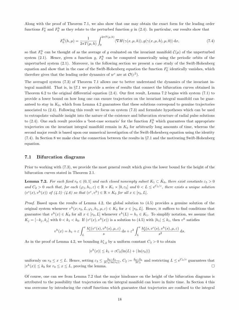
Lemma 7.2. For each fixed r0 ∈ (0, 1] and each closed nonempty subset K1 ⊂ K0, there exist constants ε5 > 0

and C2 > 0 such that, for each (ϕ1, h1, ε) ∈ R ×K1 × [0, ε5] and 0 < L ≤ eC2/ε, there exists a unique solution

(vc(x), vh(x)) of (4.5)–(4.6) so that (vc, vh) ∈ R×K0 for all x ∈ [r0, L].

Proof. Based upon the results of Lemma 4.2, the global solution to (4.5) provides a genuine solution of the

original system whenever vh(x; r0, L, ϕ1, h1, µ, ε) ∈ K0 for x ∈ [r0, L]. Hence, it suffices to find conditions that

guarantee that vh(x) ∈ K0 for all x ∈ [r0, L] whenever vh(L) = h1 ∈ K1. To simplify notation, we assume that

Kj = [−kj , kj ] with 0 < k1 < k0. If (vc(x), vh(x)) is a solution to (4.5) with |h1| ≤ k1, then vh satisfies

vh(x) = h1 + ε

∫ x

L

he1(vc(s), vh(s), µ, ε)

sds+ ε2

∫ x

L

he2(s, vc(s), vh(s), µ, ε)

s2ds.

As in the proof of Lemma 4.2, we bounding he1,2 by a uniform constant C3 > 0 to obtain

|vh(x)| ≤ k1 + εC3(ln(L) + | ln(r0)|)

uniformly on r0 ≤ x ≤ L. Hence, setting ε3 ≤ k0−k12C3| ln(r0)| , C2 := k0−k1

2C3and restricting L ≤ eC2/ε guarantees that

|vh(x)| ≤ k0 for r0 ≤ x ≤ L, proving the lemma.

Of course, one can see from Lemma 7.2 that the major hindrance on the height of the bifurcation diagrams is

attributed to the possibility that trajectories on the integral manifold can leave in finite time. In Section 4 this

was overcome by introducing the cutoff functions which guarantee that trajectories are confined to the integral

18

x

wh

wh0

-d

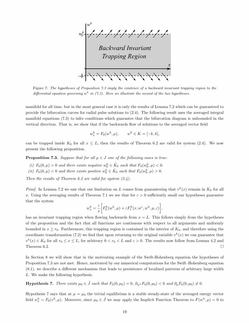
Figure 7: The hypotheses of Proposition 7.3 imply the existence of a backward invariant trapping region to the

differential equation governing wh in (7.3). Here we illustrate the second of the two hypotheses.

manifold for all time, but in the most general case it is only the results of Lemma 7.2 which can be guaranteed to

provide the bifurcation curves for radial pulse solutions to (2.4). The following result uses the averaged integral

manifold equations (7.3) to infer conditions which guarantee that the bifurcation diagram is unbounded in the

vertical direction. That is, we show that if the backwards flow of solutions to the averaged vector field

whx = F0(wh, µ), wh ∈ K = [−k, k],

can be trapped inside K0 for all x ≤ L, then the results of Theorem 6.2 are valid for system (2.4). We now

present the following proposition.

Proposition 7.3. Suppose that for all µ ∈ J one of the following cases is true:

(i) F0(0, µ) > 0 and there exists negative wh0 ∈ K0 such that F0(wh0 , µ) < 0.

(ii) F0(0, µ) < 0 and there exists positive wh0 ∈ K0 such that F0(wh0 , µ) > 0.

Then the results of Theorem 6.2 are valid for system (2.4).

Proof. In Lemma 7.2 we saw that our limitation on L comes from guaranteeing that vh(x) remain in K0 for all

x. Using the averaging results of Theorem 7.1 we see that for ε > 0 sufficiently small our hypotheses guarantee

that the system

whx =ε

x

[Fh0 (wh, µ) + εFh1 (x,wc, wh, µ, ε)

],

has an invariant trapping region when flowing backwards from x = L. This follows simply from the hypotheses

of the proposition and the fact that all functions are continuous with respect to all arguments and uniformly

bounded in x ≥ r0. Furthermore, this trapping region is contained in the interior of K0, and therefore using the

coordinate transformation (7.2) we find that upon returning to the original variable vh(x) we can guarantee that

vh(x) ∈ K0 for all r0 ≤ x ≤ L, for arbitrary 0 < r0 < L and ε > 0. The results now follow from Lemma 4.2 and

Theorem 6.2.

In Section 8 we will show that in the motivating example of the Swift-Hohenberg equation the hypotheses of

Proposition 7.3 are not met. Hence, motivated by our numerical computations for the Swift–Hohenberg equation

(8.1), we describe a different mechanism that leads to persistence of localized patterns of arbitrary large width

L. We make the following hypothesis.

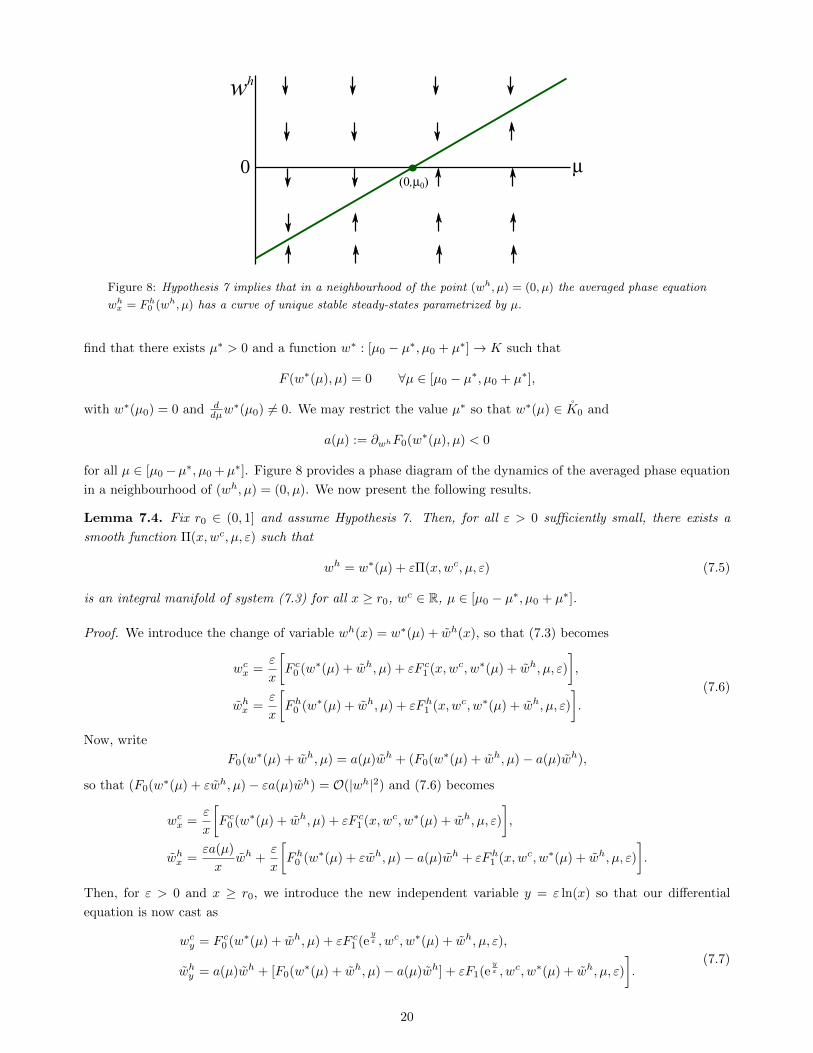
Hypothesis 7. There exists µ0 ∈ J such that F0(0, µ0) = 0, ∂whF0(0, µ0) < 0 and ∂µF0(0, µ0) 6= 0.

Hypothesis 7 says that at µ = µ0 the trivial equilibrium is a stable steady-state of the averaged energy vector

field whx = F0(vh, µ). Moreover, since µ0 ∈ J we may apply the Implicit Function Theorem to F (wh, µ) = 0 to

19

m

h

0

wh

(0,m0)

Figure 8: Hypothesis 7 implies that in a neighbourhood of the point (wh, µ) = (0, µ) the averaged phase equation

whx = Fh

0 (wh, µ) has a curve of unique stable steady-states parametrized by µ.

find that there exists µ∗ > 0 and a function w∗ : [µ0 − µ∗, µ0 + µ∗]→ K such that

F (w∗(µ), µ) = 0 ∀µ ∈ [µ0 − µ∗, µ0 + µ∗],

with w∗(µ0) = 0 and ddµw

∗(µ0) 6= 0. We may restrict the value µ∗ so that w∗(µ) ∈ K0 and

a(µ) := ∂whF0(w∗(µ), µ) < 0

for all µ ∈ [µ0−µ∗, µ0 +µ∗]. Figure 8 provides a phase diagram of the dynamics of the averaged phase equation

in a neighbourhood of (wh, µ) = (0, µ). We now present the following results.

Lemma 7.4. Fix r0 ∈ (0, 1] and assume Hypothesis 7. Then, for all ε > 0 sufficiently small, there exists a

smooth function Π(x,wc, µ, ε) such that

wh = w∗(µ) + εΠ(x,wc, µ, ε) (7.5)

is an integral manifold of system (7.3) for all x ≥ r0, wc ∈ R, µ ∈ [µ0 − µ∗, µ0 + µ∗].

Proof. We introduce the change of variable wh(x) = w∗(µ) + wh(x), so that (7.3) becomes

wcx =ε

x

[F c0 (w∗(µ) + wh, µ) + εF c1 (x,wc, w∗(µ) + wh, µ, ε)

],

whx =ε

x

[Fh0 (w∗(µ) + wh, µ) + εFh1 (x,wc, w∗(µ) + wh, µ, ε)

].

(7.6)

Now, write

F0(w∗(µ) + wh, µ) = a(µ)wh + (F0(w∗(µ) + wh, µ)− a(µ)wh),

so that (F0(w∗(µ) + εwh, µ)− εa(µ)wh) = O(|wh|2) and (7.6) becomes

wcx =ε

x

[F c0 (w∗(µ) + wh, µ) + εF c1 (x,wc, w∗(µ) + wh, µ, ε)

],

whx =εa(µ)

xwh +

ε

x

[Fh0 (w∗(µ) + εwh, µ)− a(µ)wh + εFh1 (x,wc, w∗(µ) + wh, µ, ε)

].

Then, for ε > 0 and x ≥ r0, we introduce the new independent variable y = ε ln(x) so that our differential

equation is now cast as

wcy = F c0 (w∗(µ) + wh, µ) + εF c1 (eyε , wc, w∗(µ) + wh, µ, ε),

why = a(µ)wh + [F0(w∗(µ) + wh, µ)− a(µ)wh] + εF1(eyε , wc, w∗(µ) + wh, µ, ε)

].

(7.7)

20

Hence, we are now in the appropriate form to apply [7, Theorem 2.2] to see that there exists a smooth, uniformly

bounded function Π(y, wc, µ, ε) such that

wh = Π(y, wc, µ, ε)

is an integral manifold for (7.7). Moreover, from [7, Theorem 2.2] we have that Π(y, wc, µ, 0) = 0 for all (y, wc, µ).

Therefore, tracing back all of our coordinate transformations we arrive at the integral manifold for (7.3) in the

form (7.5) given by

Π(x,wc, µ, ε) := ε−1Π(ε ln(x), wc, µ, ε),

which is smooth and uniformly bounded. This completes the proof.

Corollary 7.5. Fix r0 ∈ (0, 1] and assume Hypothesis 7. There exists ε6 > 0 such that for each L > 1,

µ ∈ [µ0 − µ∗, µ0 + µ∗], ϕ1 ∈ R, and ε ∈ [0, ε6], then the solution (vc(x), vh(x)) ∈ R×K satisfying

vc(L) = ϕ1, vh(L) = w∗(µ) + εΠ(L,ϕ1, µ, ε) + εWh(L,ϕ1, w∗(µ) + εΠ(L,ϕ1, µ, ε)µ).

where Wh is defined in (7.14), is such that vh(x) ∈ K0 for all x ∈ [r0, L].

Proof. From Lemma 7.5 we may obtain a solution to (7.3) by restricting wh = w∗(µ) + εΠ(x,wc, µ, ε) and

inspecting the resulting one-dimensional non-autonomous differential equation

wcx =ε

x

[F c0 (w∗(µ) + εΠ(x,wc, µ, ε), µ) + F c1 (x,wc, w∗(µ) + εΠ(x,wc, µ, ε), µ, ε)

].

Smoothness of the differential equation, and uniform boundedness with respect to wc imply the existence of a

solution for all x ∈ [r0, L] with the boundary condition wc(L) = ϕ′1 ∈ R, for each L > 1. Furthermore, using

the invertible change of variables introduced in Theorem 7.1, we can trace back these changes of variable to the

original variables (vc, vh) so that

vc(x) = x+ wc(x) + εW c(x,wc(x), w∗(µ) + εΠ(x,wc(x), µ, ε), µ),

vh(x) = w∗(µ) + εΠ(x,wc(x), µ, ε) + εW s(x,wc(x), w∗(µ) + εΠ(x,wc(x), µ, ε), µ).

Then, at x = L we have

vc(L) = L+ ϕ′1 + εW c(L,ϕ′1, w∗(µ) + εΠ(L,ϕ′1, µ, ε), µ).

For all L > 1 and ε ≥ 0 sufficiently small, the function

ϕ′1 7→ L+ ϕ′1 + εW c(L,ϕ′1, w∗(µ) + εΠ(L,ϕ′1, µ, ε), µ),

is surjective from R to R, and therefore, for all ϕ1 ∈ R, there exists a choice of ϕ′1 ∈ R such that vc(L) = ϕ1

when wc(L) = ϕ′1. This confirms the boundary conditions at x = L and concludes the proof.

Lemma 7.6. Assume Hypotheses 1-7 are met and we further have the following:

(i) There exists ϕ ∈ S1 such that (ϕ, µ0) ∈ Γ.

(ii) ∂ϕG0(ϕ, 0, µ0) 6= 0 for some (ϕ, µ0) ∈ Γ (i.e. the point (ϕ, µ0) is not a saddle-node unfolded in ϕ).

Then, for ε ≥ 0 sufficiently small and each ϕ0 ∈ {0, π}, the following holds: there exists a sequence {(Lϕ0n , µϕ0

n )}∞n=1

with Lϕ0n → ∞ monotonically so that at µ = µϕ0

n the differential equation (2.4) admits radial pulse solutions,

un(x;ϕ0), with the property that |un(x;ϕ0)| → ∞ monotonically.

Proof. This proof proceeds in a similar way to that of the proof of Theorem 6.2 in that we must match solutions

at x = r0 and x = L, and therefore we will primarily focus on what is different in our current situation. From

our assumptions, we can locally parametrize a neighbourhood of (ϕ, µ0) ∈ Γ in Γ as (ϕ(s), µ(s)) ∈ Γ, for a small

21

parameter s so that µ(0) = 0 and µ′(0) 6= 0. Hence, the function s 7→ µ(s) is locally surjective onto an open,

connected, neighbourhood of µ0 ∈ J .

The major difference from the proof of Theorem 6.2 is that we now assume that (Φc,Φh)(x; r0, L, ϕ1, µ, ε) is a

solution on the integral manifold satisfying the conclusions of Corollary 7.5 satisfying the boundary conditions

Φc(L; r0, L, ϕ1, µ, ε) = ϕ1, Φh(L; r0, L, ϕ1, µ, ε) = w∗(µ) +O(ε),

for some ϕ1 ∈ R and Φc(r0; r0, L, ϕ1, µ, ε) again satisfying (4.7). Thus, the matching condition (6.4) at x = r0

remains unchanged, and can again be solved for fixed r0 > 0 sufficiently small to obtain the existence a unique

function (a∗0, b∗0, h∗0)(L,ϕ0, ϕ1, µ, ε) defined for all sufficiently small ε > 0, large L > 0, ϕ0 ∈ {0, π} and arbitrary

(ϕ1, µ), smooth in the arguments (L,ϕ1, µ, ε), and given by

(a∗0, b∗0, h∗0)(L,ϕ0, ϕ1, µ, ε, s) = (0, 0,Φh(r0; r0, L, ϕ1, µ, ε)) +O(e−ηL + ε),

and again satisfying (6.6).

Now, (6.9) becomes

ϕ1 = ϕ(s) + 2πn

+ zΓ(L, ϕ(s), vsf (L; r0, L, b∗0(L,ϕ0, ϕ1, µ, ε), ϕ1, µ, ε), µ(s), ε)

∂G0

∂ϕ(ϕ(s), 0, µ(s)),

µ = µ(s) + zΓ(L, ϕ(s), b∗0(L,ϕ0, ϕ1, µ, ε), ϕ1, µ, ε), µ(s), ε)∂G0

∂µ(ϕ(s), 0, µ(s)),

w∗(µ) +O(ε) = zh(L, ϕ(s), b∗0(L,ϕ0, ϕ1, µ, ε), ϕ1, µ, ε), µ(s), ε),

(7.8)

where (ϕ(s) + 2πn, µ(s)) ∈ Γlift for every n ∈ N. All error bounds remain identical to those in the proof of

Theorem 6.2, and therefore we define the function F2 : R3 → R3 by

F2(ϕ1, µ, s) =

ϕ1 − ϕ(s)− 2πn

µ− µ(s)

w∗(µ)

+O(e−ηL + ε),

so that roots of F2 are exactly the solutions to (7.8) evaluated at b∗0(L,ϕ0, ϕ1, µ, ε), where we consider (L,ϕ0, ε, n)

to be parameters. Proceeding as before, we take w2 = (ϕ(0) + 2πn, µ0, 0) and A2 to be the matrix

A2 =

1 0 0

0 1 −µ′(0)

0 0 (w∗)′(µ0)

,which is invertible since (w∗)′(µ0) 6= 0. Since µ(0) = 0 and w∗(µ0) = 0 this then gives

F2(w2) = O(e−ηL + ε) =⇒ ‖A−12 F2(w2)‖ = O(e−ηL + ε),

and as before we further have

‖1−A−12 DF2(w)‖ = O(e−ηL + ε+ s+ µ), (7.9)

where the O(s + µ) term comes from the smooth properties of (ϕ(s), ˜µ(s)) and w∗(µ) with respect to s and µ,

respectively. Hence, taking κ = 12 and ρ > 0 sufficiently small to restrict the size of the O(s+µ) in (7.9), we can

apply Theorem 6.1 to obtain the existence a unique function (ϕ∗1, µ∗, s∗)(L,ϕ0, ε, n) defined for all sufficiently

small ε > 0, large L > 0, ϕ0 ∈ {0, π} and arbitrary n ∈ N, smooth in the arguments (L, ε), and given by

(ϕ∗1, µ∗, s∗)(L,ϕ0, ε, n) = (ϕ(0) + 2πn, µ0, 0) +O(e−ηL + ε).

Now, we again follow as in the proof of Theorem 6.2 to solve (6.4a), which requires solving

Φc(r0; r0, L, ϕ∗1(L,ϕ0, ε, n), µ∗(L,ϕ0, ε, n), ε) + r0 − ϕ0 +O(r0a

∗0(L,ϕ0, ε, s) + e−ηL + ε) = 0.

22

Similar manipulations to that of Theorem 6.2 give

ϕ(0) + 2πn− ϕ0 − L+ gc(L, µ, ε) +O(e−ηL + ε) = 0, (7.10)

where we recall that gc(L, µ, ε) = O(ε ln(L)). Then, as in the proof of Theorem 2.1, the left-hand-side of (7.10)

is unbounded in L and is monotonically decreasing for all L sufficiently large. Hence, for each n sufficiently

large, we can apply the Intermediate Value Theorem to obtain a function L(r0, n, ε), such that L(ϕ0, ε, n)→∞as n → ∞, which satisfies (7.10). We note that for each sufficiently small ε > 0 we have obtained a discrete

sequence, Lϕ0n = L(ϕ0, ε, n), of radial pulse solutions to (2.4) at µ = µ∗(L(ϕ0, ε, n), ϕ0, ε, n). Moreover, as

n→∞ we also have Lϕ0n →∞ monotonically, thus giving that |un(x;ϕ0)| → ∞ monotonically. This completes

the proof.

7.2 Proof of Theorem 7.1

The proof of Theorem 7.1 will be broken down throughout this subsection in an effort to clarify the proof by

presenting some necessary preliminary results. To begin, let vc(x) = x+ vc(x), so that we obtain

vcx = 1 + vcx,

and therefore (7.1) becomes

vcx =ε

xhc1(x+ vc, vh, µ, ε) +

ε2

x2hc2(x, x+ vc, vh, µ, ε),

vhx =ε

xhe1(x+ vc, vh, µ, ε) +

ε2

x2he2(x, x+ vc, vh, µ, ε).

(7.11)

Note that from Lemma 4.1, all functions are 2πT (µ, vh)-periodic with respect to vc and now hc,e1 are also

2πT (µ, vh)-periodic with respect the independent variable x. This leads to the first result.

Lemma 7.7. The function Fh0 defined in (7.4) is such that

Fh0 (vh, µ) =1

2πT (µ, vh)

∫ 2πT (µ,vh)

0

he1(x+ vc, vh, µ, 0) dx.

Proof. Let us define

I(vc, vh, µ) =1

2πT (µ, vh)

∫ 2πT (µ,vh)

0

he1(x+ vc, vh, µ, 0) dx.

Following the coordinate transformations of Lemma 4.1, it is clear that

he1(x+ vc, vh, µ, 0) = 〈∇H(γ(x+ vc, µ, vh)), g(γ(x+ vc, µ, h), µ, 0)〉,

which we recall from Hypothesis 4 is 2πT (µ, vh)-periodic in x and vc. Hence, I(vh, µ) becomes

I(vc, vh, µ) =1

2πT (µ, vh)

∫ 2πT (µ,vh)

0

〈∇H(γ(x+ vc, µ, vh)), g(γ(x+ vc, µ, vh), µ, 0)〉dx.

Then, vc acts as a phase-advance and hence it is clear that I(vc, vh, µ) is independent of vc. Therefore, it follows

that I(vc, vh, µ) = Fh0 (vh, µ) for all (vh, µ), thus completing the proof.

Along with Fh0 , we will also define

F c0 (vh, µ) =1

2πT (µ, vh)

∫ 2πT (µ,vh)

0

hc1(x+ vcx, vh, µ, 0) dx. (7.12)

23

Then, we consider the functions

F c,h(x, vc, vh, µ) := hc,e1 (x+ vc, vh, µ, 0)− F c,h0 (vh, µ), (7.13)

which are 2πT (µ, vh)-periodic in x and average to zero. Following the proof of Theorem 7.1, we will return to F c0to provide an explicit form in terms of the original perturbed vector field (2.4) as was done for Fh0 in Lemma 7.7.

We now state the following lemma which details the boundedness of the functions W c,h used to perform the

averaging of the vector field (7.1).

Lemma 7.8. There exists a C > 0 such that for every r0 > 0 the functions

W c(x, vc, vh, µ) :=

∫ x

r0

F c(s, vc, vh, µ)

sds,

Wh(x, vc, vh, µ) :=

∫ x

r0

Fh(s, vc, vh, µ)

sds,

(7.14)

and their derivatives with respect to vc and vh are uniformly bounded by Cr−10 for all x ≥ r0, vc ∈ R, vh ∈ K,

and µ ∈ J .

Proof. Integrating (7.14) by parts gives

W c,h(x, vc, vh, µ) =1

x

∫ x

r0

F c,h(s, vc, vh, µ) ds+

∫ x

r0

1

s2

∫ s

r0

F c,h(t, vc, vh, µ) dtds.

Recall that the functions F c,h defined in (7.13) have zero average for each fixed vh. Hence, there exists a constant

CW > 0 such that the functions

s 7→∫ s

r0

F c(t, vc, vh, µ) dt, s 7→∫ s

r0

F c(t, vc, vh, µ) dt,

are uniformly bounded by CW for all s ≥ r0, vc ∈ R, vh ∈ K and µ ∈ J . Thus, for all x ≥ r0 we have that

|W c,h(x, vc, vh, µ)| ≤ CWr0

+ CW

∫ x

r0

1

s2ds =

CWr0

+CWr0− CW

x≤ 2CW

r0.

The estimates for the derivatives of W c,h with respect to vc and vh follow in exactly the same way since the

functions are again periodic in x for each fixed vh ∈ K.

Prior to presenting the following result, it should be noted that using the function definitions (7.13), differentiating

W c,h with respect to x gives

W c,hx (x, vc, vh, µ) =

F c,h(x, vc, vh, µ)

x=

1

x(hc,e1 (x+ vc, vh, µ, 0)− F c,h0 (vh, µ)). (7.15)

We now present the proof of Theorem 7.1.

Proof of Theorem 7.1. We will use the notation

W (x,wc, wh, µ) = [W c(x,wc, wh, µ),Wh(x,wc, wh, µ)]T

for simplicity. Then, using the invertible, near-identity change of variable(vc

vh

)=

(wc

wh

)wc + εW (x,wc, wh, µ),

we have that (vcxvhx

)= (I + εD(wc,wh)W (x,wc, wh, µ))

(wcxwhx

)+

(εW c

x(x,wc, wh, µ)

εWhx (x,wc, wh, µ)

), (7.16)

24

where I denotes the 2× 2 identity matrix. and .

Then, using (7.11) and (7.15) we can rearrange (7.16) to arrive at

(I + εD(wc,wh)W (x,wc, wh, µ))

(wcxwhx

)=ε

x

(hc1(x+ wc + εW c(x,wc, wh, µ), wh + εWh(x,wc, wh, µ), µ, ε)

he1(x+ wc + εW c(x,wc, wh, µ), wh + εWh(x,wc, wh, µ), µ, ε)

)

+ε2

x2

(hc2(x, x+ wc + εW c(x,wc, wh, µ), wh + εWh(x,wc, wh, µ), µ, ε)

he2(x, x+ wc + εW c(x,wc, wh, µ), wh + εWh(x,wc, wh, µ), µ, ε)

)

− ε

x

(hc1(x+ wc, wh, µ, 0)

he1(x+ wc, wh, µ, 0)

)

+ε

x

(F c0 (wh, µ)

Fh0 (wh, µ)

).

(7.17)

From Lemma 7.8 we have that D(wc,wh)W (x,wc, wh, µ) is uniformly bounded for x ≥ r0, and therefore for ε ≥ 0

sufficiently small we have that (I + εD(wc,wh)W (x,wc, wh, µ)) is invertible for all (x,wc, wh, µ). Hence, we may

apply (I + εD(wc,wh)W (x,wc, wh, µ))−1 to both sides of (7.17) to obtain(wcxwhx

)=ε

x(I + εD(wc,wh)W (x,wc, wh, µ))−1

(F c0 (wh, µ) + F c1 (x,wc, wh, µ, ε)

Fh0 (wh, µ) + Fh1 (x,wc, wh, µ, ε)

),

where we have introduced the function F c,h1 to compactly write the right-hand-side of (7.17), and note that

F c,h1 (x,wc, wh, µ, ε) = O(ε).

Finally, remarking that [(I + εD(wc,wh)W (x,wc, wh, µ))−1 − I] = O(ε), we have(wcxwhx

)=ε

x

(F c0 (wh, µ)

Fh0 (wh, µ)

)+ε

x[(I + εD(wc,wh)W (x,wc, wh, µ))−1 − I]

(F c0 (wh, µ)

Fh0 (wh, µ)

)︸ ︷︷ ︸

O(ε2)

+ε

x(I + εD(wc,wh)W (x,wc, wh, µ))−1

(F c1 (x,wc, wh, µ, ε)

Fh1 (x,wc, wh, µ, ε)

)︸ ︷︷ ︸

O(ε2)

.

Hence, defining the functions(F c1 (x,wc, wh, µ, ε)

Fh1 (x,wc, wh, µ, ε)

)= ε−1[(I + εD(wc,wh)W (x,wc, wh, µ))−1 − I]

(F c0 (wh, µ)

Fh0 (wh, µ)

)

+ (I + εD(wc,wh)W (x,wc, wh, µ))−1

(F c1 (x,wc, wh, µ, ε)

Fh1 (x,wc, wh, µ, ε)

),

shows that our differential equation is now in the form of (7.3). Note F c,h1 are well-defined, smooth and uniformly

bounded when ε ≤ r20. This completes the proof.

Having now proved Theorem 7.1, we now provide an explicit form for the function F c0 in terms of the original

perturbed vector field (2.4).. Recall that in (7.12) we have that

F c0 (vh, µ) =1

2πT (µ, vh)

∫ 2πT (µ,vh)

0

hc1(x+ vcx, vh, µ, 0) dx.

Furthermore, since the periodic orbits γ(x, µ, h) of the unperturbed system (2.1) depend smoothly on h, we find

that γh(x, µ, h) (the partial derivative of γ(x, µ, h) with respect to h) is a solution to the variational equation

25

ux = fu(γ(x, µ, h))u. Furthermore, γh(0, µ, h) ∈ Fix(R), or equivalently, γh(x, µ, h) = Rγh(−x, µ, h) for all

(x, µ, h).

From the discussion following Hypothesis 4, standard Floquet Theory tells us that for each (x, µ, h) the set

{γx(x, µ, h), ps(x, µ, h), pu(x, µ, h), γh(x, µ, h)}

is a linearly-independent, spanning set of R4. Then, we define a smooth function ψ(x, µ, h) so that ψ is orthogonal

to span{ps, pu, γh} with |ψ(x, µ, h)| = 1 for each (x, µ, h). This leads to the following result detailing the precise

expression for F c0 in terms of the perturbed vector field (2.4).

Lemma 7.9. The function F c0 defined in (7.12) is such that

F c0 (vh, µ) =1

2πT (µ, vh)

∫ 2πT (µ,vh)

0

〈ψ(x, µ, vh), g(γ(x, µ, vh))〉〈ψ(x, µ, vh), γx(x, µ, vh)〉 dx.

Proof. In Lemma 4.1 we introduced the change of variable

u = Q(v) = γ(vc, µ, vh) + vsps(vc, µ, vh) + vupu(vc, µ, vh) + h.o.t., (7.18)

so that when ε = 0 we have vu = 0 and vs = 0 parametrize the strong stable and strong unstable fibres of

γ(vc, µ, vh), respectively. Differentiating (7.18) results in

f(Q(v)) +ε

xg(Q(v), µ, ε) = γx(vc, µ, vh)vcx + γh(vc, µ, vh)vhx + ps(vc, µ, vh) + pu(vc, µ, vh) + h.o.t., (7.19)

where we have used the fact that u is a solution of (2.4). Then, to obtain the form of the vcx equation in (4.3) we

take the inner product with ψ of both sides of (7.19) and divide by 〈ψ(x, µ, vh), γx(x, µ, vh)〉. It should be noted

that 〈ψ(x, µ, vh), γx(x, µ, vh)〉 never vanishes due to the linear independence of the set {γx, ps, pu, γh} and the

fact that ψ is orthogonal to span{ps, pu, γh}. This process is exactly how the form for the vcx equation is derived

to obtain it as stated in (4.3). Particularly, following the coordinate transformations of Lemma 4.1 we have that

hc1(vc, vh, µ, ε) =〈ψ(vc, µ, vh), g(Q(vc, 0, 0, vh))〉〈ψ(vc, µ, vh), γx(vc, µ, vh)〉 .

Now, using the fact that Q(vc, 0, 0, vh) = γ(vc, µ, vh), from (7.12) we have that F c0 (vh, µ) is in the form stated

in the lemma.

In Section 8 we will use Lemma 7.9 to show that when considering the motivating case of the Swift–Hohenberg

equation we find that F c0 vanishes for all (vh, µ) ∈ K × J .

8 Application to the Swift-Hohenberg Equation

We now apply our results to the Swift–Hohenberg equation (1.1). Recall that radial steady-states of the Swift–

Hohenberg equation posed on Rn satisfy the system

0 = −(

1 +n− 1

x∂x + ∂xx

)2

U − µU + νU2 − U3, (8.1)

where we denote the radial variable by x. Setting ε := n − 1, u1 = U , u2 = ∂xu1, u3 = (1 + εx∂x + ∂xx)u1 and

u4 = ∂xu3, equation (8.1) is equivalent to

u′1 = u2,

u′2 = u3 − u1 −ε

xu2,

u′3 = u4,

u′4 = −u3 − µu1 + νu21 − u3

1 −ε

xu4.

(8.2)

26

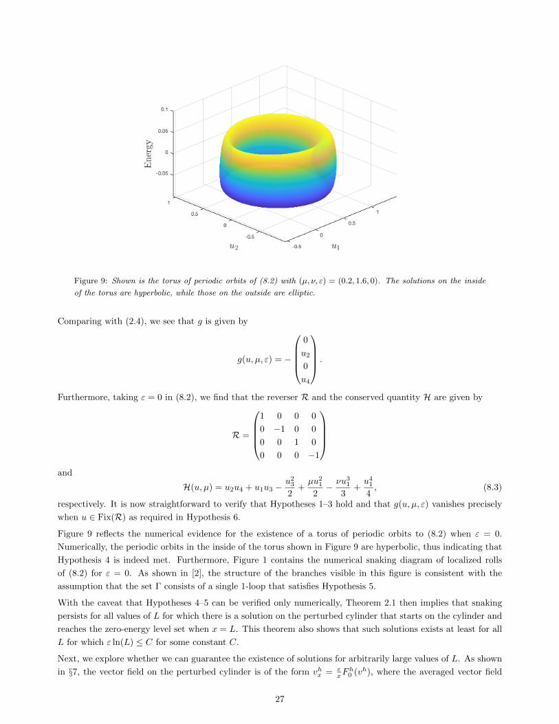
Figure 9: Shown is the torus of periodic orbits of (8.2) with (µ, ν, ε) = (0.2, 1.6, 0). The solutions on the inside

of the torus are hyperbolic, while those on the outside are elliptic.

Comparing with (2.4), we see that g is given by

g(u, µ, ε) = −

0

u2

0

u4

.

Furthermore, taking ε = 0 in (8.2), we find that the reverser R and the conserved quantity H are given by

R =

1 0 0 0

0 −1 0 0

0 0 1 0

0 0 0 −1

and

H(u, µ) = u2u4 + u1u3 −u2

3

2+µu2

1

2− νu3

1

3+u4

1

4, (8.3)

respectively. It is now straightforward to verify that Hypotheses 1–3 hold and that g(u, µ, ε) vanishes precisely

when u ∈ Fix(R) as required in Hypothesis 6.

Figure 9 reflects the numerical evidence for the existence of a torus of periodic orbits to (8.2) when ε = 0.

Numerically, the periodic orbits in the inside of the torus shown in Figure 9 are hyperbolic, thus indicating that

Hypothesis 4 is indeed met. Furthermore, Figure 1 contains the numerical snaking diagram of localized rolls

of (8.2) for ε = 0. As shown in [2], the structure of the branches visible in this figure is consistent with the

assumption that the set Γ consists of a single 1-loop that satisfies Hypothesis 5.

With the caveat that Hypotheses 4–5 can be verified only numerically, Theorem 2.1 then implies that snaking

persists for all values of L for which there is a solution on the perturbed cylinder that starts on the cylinder and

reaches the zero-energy level set when x = L. This theorem also shows that such solutions exists at least for all

L for which ε ln(L) ≤ C for some constant C.

Next, we explore whether we can guarantee the existence of solutions for arbitrarily large values of L. As shown

in §7, the vector field on the perturbed cylinder is of the form vhx = εxF

h0 (vh), where the averaged vector field

27

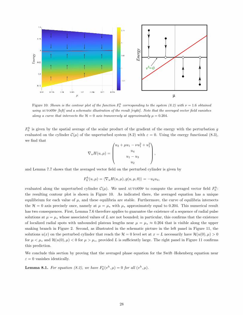
Energy

m

vh=0

Figure 10: Shown is the contour plot of the function Fh0 corresponding to the system (8.2) with ν = 1.6 obtained

using auto09p [left] and a schematic illustration of the result [right]. Note that the averaged vector field vanishes

along a curve that intersects the H = 0 axis transversely at approximately µ = 0.204.

Fh0 is given by the spatial average of the scalar product of the gradient of the energy with the perturbation g

evaluated on the cylinder C(µ) of the unperturbed system (8.2) with ε = 0. Using the energy functional (8.3),

we find that

∇uH(u, µ) =

u3 + µu1 − νu2

1 + u31

u4

u1 − u3

u2

,

and Lemma 7.7 shows that the averaged vector field on the perturbed cylinder is given by

Fh0 (u, µ) = 〈∇uH(u, µ), g(u, µ, 0)〉 = −u2u4,

evaluated along the unperturbed cylinder C(µ). We used auto09p to compute the averaged vector field Fh0 :

the resulting contour plot is shown in Figure 10. As indicated there, the averaged equation has a unique

equilibrium for each value of µ, and these equilibria are stable. Furthermore, the curve of equilibria intersects

the H = 0 axis precisely once, namely at µ = µ∗ with µ∗ approximately equal to 0.204. This numerical result

has two consequences. First, Lemma 7.6 therefore applies to guarantee the existence of a sequence of radial pulse

solutions at µ = µ∗ whose associated values of L are not bounded; in particular, this confirms that the existence

of localized radial spots with unbounded plateau lengths near µ = µ∗ ≈ 0.204 that is visible along the upper

snaking branch in Figure 2. Second, as illustrated in the schematic picture in the left panel in Figure 11, the

solutions u(x) on the perturbed cylinder that reach the H = 0 level set at x = L necessarily have H(u(0), µ) > 0

for µ < µ∗ and H(u(0), µ) < 0 for µ > µ∗, provided L is sufficiently large. The right panel in Figure 11 confirms

this prediction.

We conclude this section by proving that the averaged phase equation for the Swift–Hohenberg equation near

ε = 0 vanishes identically.

Lemma 8.1. For equation (8.2), we have F c0 (vh, µ) = 0 for all (vh, µ).

28

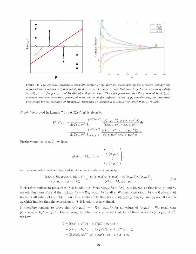
Energy

m

vh=0

50 100 150 200 250 300 350-4

-3

-2

-1

0

1

2

3

410-3

= 0.195= 0.1975= 0.2004= 0.2025= 0.205

Figure 11: The left panel contains a schematic picture of the averaged vector field on the perturbed cylinder and

representative solutions u(x) that satisfy H(u(L), µ) = 0 for large L: note that these trajectories necessarily satisfy

H(u(0), µ) > 0 for µ < µ∗ and H(u(0), µ) < 0 for µ > µ∗. The right panel contains the graphs of H(u(x), µ),

averaged over one wave-train period, of radial pulses at five different values of µ, corroborating the theoretical

predictions for the evolution of H(u(x), µ) depending on whether µ is smaller or larger than µ∗ ≈ 0.204.

Proof. We proved in Lemma 7.9 that F c0 (vh, µ) is given by

F c0 (vh, µ) =1

2πT (µ, vh)

∫ 2πT (µ,vh)

0

〈ψ(x, µ, vh), g(γ(x, µ, vh))〉〈ψ(x, µ, vh), γx(x, µ, vh)〉 ds

=1

2πT (µ, vh)

∫ πT (µ,vh)

−πT (µ,vh)

〈ψ(x, µ, vh), g(γ(x, µ, vh))〉〈ψ(x, µ, vh), γx(x, µ, vh)〉 ds.

Furthermore, using (8.2), we have

g(γ(x, µ, h), µ, ε) = −

0

γ2(x, µ, h)

0

γ4(x, µ, h)

,

and we conclude that the integrand in the equation above is given by

〈ψ(x, µ, h), g(γ(x, µ, h), µ, ε)〉〈ψ(x, µ, h), γx(x, µ, h)〉 =

ψ2(x, µ, h)γ2(x, µ, h) + ψ4(x, µ, h)γ4(x, µ, h)

〈ψ(x, µ, h), γx(x, µ, h)〉 . (8.4)

It therefore suffices to prove that (8.4) is odd in x. Since γ(x, µ, h) = Rγ(−x, µ, h), we see that both γ2 and γ4

are odd functions of x and that γx(x, µ, h) = −Rγx(−x, µ, h) for all x. We claim that ψ(x, µ, h) = −Rψ(−x, µ, h)

holds for all values of (x, µ, h). If true, this would imply that 〈ψ(x, µ, h), γx(x, µ, h)〉, ψ2, and ψ4 are all even in

x, which implies that the expression in (8.4) is odd in x as claimed.

It therefore remains to prove that ψ(x, µ, h) = −Rψ(−x, µ, h) for all values of (x, µ, h). We recall that

pu(x, µ, h) = Rps(−x, µ, h). Hence, using the definition of ψ, we see that, for all fixed constants (c1, c2, c3) ∈ R3,

we have

0 = 〈ψ(x), c1ps(x) + c2p

u(x) + c3γh(x)〉= 〈ψ(x), c1Rpu(−x) + c2Rps(−x) + c3Rγh(−x)〉= 〈Rψ(x), c1p

u(−x) + c2ps(−x) + c3γh(−x)〉,

29

where we have suppressed the dependence of all functions on (µ, h) for notational convenience. Since (c1, c2, c3)

were arbitrary and ψ(x) spans the orthogonal compliment of span{ps(x), pu(x), γh(x)} for all (x, µ, h), it follows

that

Rψ(x) = ±ψ(−x) =⇒ ψ(x) = ±Rψ(−x),

for every x, since ψ is smooth and is such that |ψ(x, µ, h)| = 1 for all (x, µ, h). Now, recall that γh(0) ∈ Fix(R),

and, furthermore, we have

ps(0) + pu(0) = ps(0) +Rps(0) ∈ Fix(R).

Linear independence of the set {ps(x), pu(x), γh(x)} for all x coupled with the fact that Fix(R) is two-dimensional

then implies that

Fix(R) = span{ps(0) + pu(0), γh(0)}.

Then, by definition of ψ(x), for all (c1, c2) ∈ R2 we have

〈ψ(0), c1(ps(0) + pu(0)) + c2γh(0)〉 = 0,

and hence we must have that ψ(0) ∈ Fix(−R). Therefore, ψ(x) = −Rψ(−x) and the lemma is proved.

9 Discussion

In this paper, we analyzed the existence and bifurcation structure of localized roll solutions to a class of singularly

perturbed ODEs. The class of ODEs was motivated by the system (1.3), whose solutions correspond to stationary

radial spots of the Swift–Hohenberg equation (1.2) posed on Rn. The two key differences between n = 1 and

n > 1 are that (1.3) no longer possesses a conserved quantity when n > 1 and that the term 1/x that becomes

effective for n > 1 is not integrable on [1,∞). Through a perturbation analysis near n = 1, we were able to

attribute the breakup of the snaking structure in dimensions n > 1 to these differences: the lack of a conservative

quantity allows trajectories to track the entire invariant cylinder of periodic orbits, and the non-integrability of

the perturbation allows solutions on the invariant cylinder to leave the cylinder through its top or bottom

in finite time. Our analysis explains why the lower branch shown in Figure 2 for radial spots of the planar

Swift–Hohenberg equation is bounded.

In addition, our description of the flow on the invariant perturbed cylinder of periodic orbits via averaging

provided an explanation for the vertical asymptote of the upper snaking branch near µ = 0.204. Specifically, we

proved that, if the averaged vector field on the cylinder admits solutions that stay on the cylinder for all times

and reach the periodic orbit that has zero energy, then the full system has radial pulses for each sufficiently

large roll plateau length. We showed numerically that the averaged equation belonging to the Swift–Hohenberg

equation has an equilibrium in the zero energy level set when µ is near 0.204.

Our analysis does not explain the precise structure of the branches shown in Figure 2 for the planar Swift–

Hohenberg equation. In particular, we can explain neither the existence of an intermediate stack of isolas nor

the fact the upper snaking branch forms a connected curve. We believe that the specific shape of the snaking

diagram is determined by the behavior of solutions away from the invariant cylinder of periodic orbits and will

therefore likely depend on the global dynamics rather than local properties near the cylinder of rolls and the

stable manifold of the origin.

Finally, we observed numerically that the vertical asymptote µ = µ∗ of the upper snaking branch for the Swift–

Hohenberg equation with n > 1 agrees, to numerical accuracy, with the Maxwell point. As pointed out in the

last section, the conditions that give, respectively, the vertical asymptote and the Maxwell point differ, and it is

not clear to us why their difference vanishes for all values of ν.

30

Acknowledgements. Bramburger was supported by an NSERC PDF, Altschuler was supported by the NSF

through grant DMS-1439786, Avery, Carter, and Sangsawang were supported by the NSF through grant DMS-

1148284, and Sandstede was partially supported by the NSF through grant DMS-1408742.

References

[1] T. Aougab, M. Beck, P. Carter, S. Desai, B. Sandstede, M. Stadt, and A. Wheeler. Isolas versus snaking of

localized rolls, J. Dyn. Differ. Equ., at press.

[2] M. Beck, J. Knobloch, D. Lloyd, B. Sandstede, and T. Wagenknecht. Snakes, ladders, and isolas of localized

patterns, SIAM J. Math. Anal. 41, (2009) 936-972.

[3] J. Burke and E. Knobloch. Localized states in the generalized Swift–Hohenberg equation, Phys. Rev. E 73,

(2006) 056211.

[4] P. Coullet, C. Riera, and C. Tresser. Stable static localised structures in one dimension, Phys. Rev. Lett.

84, (2000) 3069-3072.

[5] N. Fenichel. Geometric singular perturbation theory for ordinary differential equations, J. Differ. Equations

31, (1979) 53-98.

[6] M. Groves, D. Lloyd, and A. Stylianou. Pattern formation on the free surface of a ferrofluid: spatial dynamics

and homoclinic bifurcation, Phys. D. 350, (2017) 1-12.

[7] J. Hale. Ordinary Differential Equations, 2nd Ed., Robert E. Kreiger Publishing Company, Florida, 1980.

[8] C. Kuehn. Multiple Time Scale Dynamics, volume 191 of Applied Mathematical Sciences. Springer-Verlag,

New York, 2015.

[9] D. Lloyd and H. OFarrell. On localised hotspots of an urban crime model, Phys. D. 253, (2013) 23-39.

[10] D. Lloyd and B. Sandstede. Localized radial solutions of the Swift–Hohenberg equation, Nonlinearity 22,

(2009) 485-524.

[11] D. Lloyd, B. Sandstede, D. Avitabile, and A. Champneys. Localized hexagon patterns in the planar Swift–

Hohenberg equation, SIAM J. Appl. Dyn. Syst. 7, (2008) 1049-1100.

[12] S. McCalla and B. Sandstede. Snaking of radial solutions of the multi-dimensional Swift–Hohenberg equa-

tion: a numerical study, Phys. D. 239 (2010), 1581-1592.

[13] S. McCalla and B. Sandstede. Spots in the Swift–Hohenberg equation, SIAM J. Appl. Dyn. Syst. 12, (2013)

831-877.

[14] E. Meron. Pattern-formation approach to modelling spatially extended ecosystems, Ecol. Model. 234, (2012)

70-82.

[15] Y. Pomeau. Front motion, metastability, and subcritical bifurcations in hydrodynamics, Phys. D. 130,

(1999) 73-104.

[16] P. Parra-Rivas, D. Gomila, L. Gelens, and E. Knobloch. Bifurcation structure of localized states in the

Lugiato-Lefever equation with anomalous dispersion, Phys. Rev. E 97, (2018) 042204.

[17] S. Schecter. Exchange lemmas 1: Deng’s lemma, J. Differ. Equations 245, (2008) 392-410.

31

[18] E. Sheffer, H. Yizhaq, M. Shachak, and E. Meron. Mechanisms of vegetation-ring formation in water-limited

systems, J. Theor. Bio. 273, (2011) 138-146.

[19] P. Woods and A. Champneys. Heteroclinic tangles and homoclinic snaking in the unfolding of a degenerate

reversible Hamiltonian-Hopf bifurcation, Phys. D. 129, (1999) 147-170.

32