Pattern Recognition 40 (2007) 19–32www.elsevier.com/locate/patcog

Image classification with the use of radial basis function neural networksand the minimization of the localized generalization error

Wing W.Y. Nga,b,∗, Andres Doradoc, Daniel S. Yeunga,b, Witold Pedryczd, Ebroul Izquierdoc

aDepartment of Computing, The Hong Kong Polytechnic University, ChinabMedia and Life Science Computing Lab, Shenzhen Graduate School, Harbin Institute of Technology, China

cDepartment of Electronic Engineering, Queen Mary, University of London, UKdDepartment of Electrical and Computer Engineering, University of Alberta, Canada

Received 31 October 2005; accepted 6 July 2006

Abstract

Image classification arises as an important phase in the overall process of automatic image annotation and image retrieval. In this study,we are concerned with the design of image classifiers developed in the feature space formed by low level primitives defined in the setting ofthe MPEG-7 standard. Our objective is to investigate the discriminatory properties of such standard image descriptors and look at efficientarchitectures of the classifiers along with their design pursuits. The generalization capabilities of an image classifier are essential to itssuccessful usage in image retrieval and annotation. Intuitively, it is expected that the classifier should achieve high classification accuracyon unseen images that are quite “similar” to those occurring in the training set. On the other hand, we may assume that the performance ofthe classifier could not be guaranteed in the case of images that are very much dissimilar from the elements of the training set. To followthis observation, we develop and use a concept of the localized generalization error and show how it guides the design of the classifier.As image classifier, we consider the usage of the radial basis function neural networks (RBFNNs). Through intensive experimentation weshow that the resulting classifier outperforms other classifiers such as a multi-class support vector machines (SVMs) as well as “standard”RBFNNs (viz. those developed without the guidance offered by the optimization of the localized generalization error). The experimentalstudies reveal some interesting interpretation abilities of the RBFNN classifiers being related with their receptive fields.� 2006 Pattern Recognition Society. Published by Elsevier Ltd. All rights reserved.

Keywords: Image classification; Radial basis functions neural networks; MPEG-7; Support vector machines; Generalization error

1. Introduction

A vast amount of digital images are become omnipresentthese days call for an intensified effort towards buildingefficient needs for their automatic annotation and retrievalmechanisms. Classification of digital images becomesone of the fundamental activities one could view as the

∗ Corresponding author. Department of Computing, The Hong KongPolytechnic University, China. Tel.: +852 2766 4901; fax: +852 2774 0842.

E-mail addresses: cswyng@comp.polyu.edu.hk(W.W.Y. Ng), andres.dorado@elec.qmul.ac.uk (A. Dorado),csdaniel@comp.polyu.edu.hk (D.S. Yeung), pedrycz@ee.ualberta.ca(W. Pedrycz), ebroul.izquierdo@elec.qmul.ac.uk (E. Izquierdo).

0031-3203/$30.00 � 2006 Pattern Recognition Society. Published by Elsevier Ltd. All rights reserved.doi:10.1016/j.patcog.2006.07.002

fundamental prerequisite for all other image processingpursuits. In image classification we could follow the generalparadigm of pattern recognition. In pattern recognition, eachobject is described by a collection of features that forms amultidimensional space in which all discrimination activi-ties take place. Various classifiers, both linear and nonlinear,become available at this stage including support vectormachines (SVM), linear classifiers, polynomial classifiers,radial basis function neural networks (RBFNNs), fuzzyrule-based systems, etc. No matter what classifier hasbeen chosen, a formation of a suitable feature becomes ofparamount relevance. The problem of forming of the featurespace in the case of images is even more complicated. Onone hand, we have a lot of different alternatives. On the other

20 W.W.Y. Ng et al. / Pattern Recognition 40 (2007) 19–32

hand, the diversity of images contributes to the elevatedlevel of complexity and difficulty. In images, we encounter avariety of images showing different shapes, colors, texture,etc yet belonging to the same class. An image could bedescribed by an intensity of color of each pixel or even betterby some descriptors. In this study, our objective is to exploreand quantify the discriminatory properties of the MPEG-7 image descriptors in classification problems. Those areexplored in conjunction to two main categories of classifierssuch as SVMs and RBFNNs.

Unfortunately, it becomes obvious that any classifierrequiring high training accuracy may not achieve good gen-eralization capability. Since both target outputs and distri-butions of the unseen samples are unknown, it is impossibleto compute the generalization error in a direct way. Thereare two major approaches to estimate the generalizationerror, namely, analytical model and cross-validation (CV).In general, analytical models bound above the generaliza-tion error for any unseen samples and do not distinguishtrained classifiers with the same number of effective pa-rameters but different values of parameters. Thus, the errorbounds given by those models are usually loose [1]. Themajor problem of analytical models is the estimation ofthe number of effective parameters of the classifier, whichcould be solved by using the VC-dimensions [2]. The VC-dimension of a classifier is defined as the largest number ofsamples that can be shattered by this classifier [2]. How-ever, only loose bound of VC-dimensions could be foundfor nonlinear classifiers, e.g. neural networks, and this putsa severe limitation on the applicability of analytical modelsto nonlinear classifiers, except the SVM [3]. Although CVuses true target outputs for unseen samples, it is time con-suming for large datasets and CL classifiers must be trainedfor C-fold CV and L choices of classifier parameters. CVmethods estimate the expected generalization error insteadof its bound, thus they do not guarantee the finally builtclassifier to have good generalization capability [1].

In image classification, one may not expect a classifiertrained using one category of images (say, animals) to cor-rectly classify images coming from some other categories(e.g. vegetables). In this case, one may revise the train-ing dataset by adding training samples of vegetables andre-train the classifier to include the new class of images. Forexample, in our dataset we have images of cow but not air-plane, thus we could not expect the classifier trained usingour dataset to correctly recognize an airplane. It is expectedthat an image classifier work well for those classes that havebeen used to train it assuming images belonging to the sameclass are conceptually similar and such that their descriptorvalues should also be similar. That is, unseen samples simi-lar to the training samples, in terms of sup-type of distancein the feature space is smaller than a given threshold, areconsidered to be more important. Thus, in the evaluation ofthe generalization capabilities of the image classifiers, onemay ignore those images that are totally dissimilar to thoseexisting in the training set.

In general, image classification problems are multi-classclassification problems and difficult to find a classifier withgood generalization properties. In this work, we aim to findan image classifier featuring better generalization capabil-ity and interpretability with respect to domain knowledgein image classification. We concentrate on finding an opti-mal number of receptive fields for RBFNNs to classify theimages with lower generalization error to unseen images.

We organize the study in the following manner. The start-ing point is a discussion on the formation of the featurespace based upon the framework of descriptors being avail-able in the MPEG-7 standard. These issues are covered inSection 2. We provide a brief introduction to image classi-fiers in Section 3. The localized generalization error model(R∗

SM) and the corresponding approach to the selection ofthe architecture of the network are described in Sections 4and 5, respectively. We present a comprehensive suite of ex-perimental studies in Section 5. Concluding comments arecovered in Section 6.

2. MPEG-7 feature space

In this section, we elaborate on the feature space arisingwithin the framework of MPEG-7. The MPEG-7 descrip-tors are useful for low-level matching and provide a greatflexibility for a wide range of applications.

2.1. MPEG-7 descriptors

MPEG-7, formally known as multimedia content de-scription interface is an ISO/IEC standard developed bythe moving picture experts group (MPEG) for descrip-tion and search of audio and video content; refer towww.chiariglione.org/mpeg/. In contrast with the earlierstandards known as MPEG-1, MPEG-2, and MPEG-4 thatare focused on coding and representation of audio–visualcontent, On the other hand, MPEG-7 moves forward andbecomes more general by embracing a description of mul-timedia content [4].

MPEG-7 has emerged as a cornerstone of the develop-ment of a wide spectrum of applications dealing with audio,speech, video, still pictures, graphics, 3D models, and alike.In a nutshell, the MPEG-7 environment delivers a compre-hensible metadata description standard that is interoperablewith other leading standards such as SMPTE Metadata Dic-tionary, Dublin Core, EBU P/Meta, and TV Anytime; re-fer to www.ebu.ch/trev_284-mulder.pdf. Initially, MPEG-7was focused more on web-based applications and annota-tion tools (e.g. Refs. [5,6]). Nowadays, it is being drifted toother domains such as education, video surveillance, enter-tainment, medicine and biomedicine.

The ultimate objective of MPEG-7 is to provide interoper-ability among systems and applications used in generation,management, distribution, and consumption of audio–visualcontent descriptions. Such descriptions of streamed (live) or

W.W.Y. Ng et al. / Pattern Recognition 40 (2007) 19–32 21

Table 1MPEG-7 visual descriptors used to characterize still images

Color descriptors Texture descriptors Shape descriptors

Color layout Texture browsing Region-based shapeColor structure Homogeneous texture Contour-based shapeDominant color Edge histogramScalable color

stored on various media help either users or applications inidentifying, retrieving, or filtering essential audio–visual in-formation, cf. Refs. [4,7].

MPEG-7 specifies standardized descriptors and descrip-tion schemes for audio and video, as well as integratedmultimedia content. Also standardized is a description def-inition language that allows for new descriptors and de-scription schemes to be defined. MPEG-7 descriptors definesyntax and semantics of features of audio–visual content.MPEG-7 allows these descriptions to be at different per-ceptual and semantic levels. At the lowest abstraction level,such descriptors may include shape, texture, and color. Atthe highest abstraction level, they may include events, ab-stract concepts, and so forth. Table 1 presents a list of thebasic MPEG-7 visual descriptors applicable to still images.

We use the proposed feature vector structure [8] that com-bines features extracted from MPEG-7 color and texture de-scriptors. The structure keeps the original topology in orderto preserve syntax and embedded semantics on these descrip-tors. The proposed feature space is constructed using fivehistogram-based MPEG-7 color and texture descriptors [9].The color layout descriptor (CLD) effectively represents thespatial distribution of color in a very compact form by con-trolling the number of coefficients enclosed in the descrip-tor. The scalable color descriptor (SCD) is a color histogramin Hue-saturation-value color space, which is encoded by aHaar transform. The color structure descriptor (CSD) cap-tures both color content and information about the struc-ture of this content. In contrast to ordinary color histogramthis descriptor uses a sliding window to capture color dis-tributions by groups of pixels rather than by each pixel be-ing treated separately. The edge histogram descriptor (EHD)captures spatial distribution of five types of edges. Semi-global and global histograms derived from this descriptorcan be combined with other descriptors, e.g. color struc-ture, to obtain accurate matching between images of a sim-ilar semantics. The homogeneous texture descriptor (HTD)is useful to represent image data as a mosaic of homoge-neous textures. This descriptor provides a useful quantitativerepresentation of the texture by using the first and secondmoments of the energy in the frequency domain.

2.2. Selection of the MPEG-7 descriptor elements

The selection of the descriptor elements becomes an im-portant issue in defining the structure of the feature space.

This is an open and difficult problem to define an absolutelyoptimal feature space due to the lack of evaluation criteria.Furthermore, any bias towards either color or texture de-scriptors may not be appropriate. Thus, in this study, we in-tend to use a suite of descriptors which produces a balancedfeature space by including a suitable number of the textureand color descriptors. Table 2 shows the different configura-tions of color and textures components in the feature space.

As indicated in the last column (Settings), the CLD is setup to the recommended default, which includes six Y coeffi-cients and three each of Cr and Cb coefficients [9]. CSD isadjusted to 64 elements, which are calculated based on ap-proximations done when using the 184-bin descriptor. SCDis fixed to 64 by scaling the quantized representation of Haarcoefficients to obtain the desired number of bits. EHD usesits default that corresponds to 80 elements. HTD uses thefull-layer; that is 62 elements. The 140-element color and142-element texture components produce a difference of twoelements, which constitutes an acceptable balance. Conse-quently, the full-size feature vector consists of 282 elements.Afterwards, following the paradigm of pattern recognition,let us treat each image formed in the MPEG-7 feature spaceas a 282-dimensional numeric vector. The images will bedenoted as x, z, y and alike.

3. Classifiers for image classification

In this section, we discuss several selected architecturesof classifiers that are quite often encountered in image clas-sification. It is of interest to investigate their properties inthis setting and review some related development strategies.

3.1. SVMs for image classification

In image classification, a significant interest has been ex-pressed in classifiers realized as SVMs [2]. In Ref. [10],Barla et al. investigated the potential of SVMs to solve im-age classification problems. As pointed out by Jain et al.an evident advantage of SVMs classifiers lies in their capa-bilities to learn from a relatively small number of samples[11]. The class (label) of a new sample is determined bya linear combination of the kernel functions evaluated ona certain subset of the examples—the support vectors andthe input. The coefficients of the combination are obtainedas a solution to a convex optimization problem occurring atthe learning stage. The choice of the kernel relies on priorknowledge of the problem domain.

Chapelle et al. presented an approach to overcome poorlygeneralization on image classification tasks, because of thehigh dimensionality of the feature space. They used a SVMsapproach because of its good generalization performancethat is retained even when the dimension of the input spaceis very high [12]. Serrano et al. proposed an improved SVM-based approach to indoor/outdoor classification. The ap-proach uses a low-dimensional feature set in which a low

22 W.W.Y. Ng et al. / Pattern Recognition 40 (2007) 19–32

Table 2Setting of the dimensionality of the feature vector with the reference to different configurations of color and texture components in the MPEG-7 featurespace

Descriptor Number of elements Settings

CLD 12 12CSD 32 64 120 184 64SCD 16 62 64 128 256 64EHD 80 80HTD 32 62 62

dim(Color) = 140, dim(Texture) = 142

Difference in number of features 2Total number of features 282

computation complexity is achieved without compromis-ing the accuracy [13]. Yen et al. applied SVM ensemblesto adapt binary SVMs to multi-class classification and ad-dress the high computational cost for training [14]. Tsaiet al. implemented concept-based indexing by combiningSOMs and SVMs in a two-stage hybrid classifier [15]. InRef. [16] Prabhakar et al. proposed another hybrid approach.The classification of images as either picture or graphicsis performed by a combination of a rule-based tree classi-fier and a neural network classifier. Dong and Yang com-bined SVMs and kNN for hierarchical classification of webimages. A threshold strategy called “HRCut” is proposedas a way of handling the difficulty in applying traditionalstrategies (e.g. rank-based threshold) to decide the winnercategory for each image [17].

Several methods have been proposed to deal with multi-class problem using SVM [18], such as one-against-all, how-ever they are still based on binary classifications. Moreover,SVM project the images to a very high dimensional kernelspace in which one may find difficult to analyze the resultingclassifier and relate it to any domain knowledge availablewhen dealing any problems of image classification.

3.2. RBFNNs in image classification

In contrast, the RBFNNs [19,20] operate directly in the in-put space, i.e. the MPEG-7 feature space we have discussedin Section 2. In later section, we will discuss aspects of thevisualization of the receptive fields and their relationshipswith the images and MPEG-7 descriptors, in particular. Thetraining of RBFNNs consists of two major phases that isunsupervised and supervised learning. In the unsupervisedphase, one defines the number of receptive fields and thenthe clustering algorithm is used to determine the center andthe spread of the receptive field. The connections (weights)between the output of the RBFNN and receptive fields arecomputed by pseudo-inverse, which becomes possible ow-ing to the linear relationship with respect to the parametersto be estimated. The assumed performance index is viewedas the mean squared error (MSE). A selection of a suitable

number of the receptive fields of the network becomes akey architectural component to the successful performanceof the resulting RBFNN. Fig. 1 illustrates the architectureof the RBFNN. The kth output of the RBFNN is describedin the following form

f (x, k) =M∑

j=1

wjk exp

((x − uj )

T(x − uj )

−2v2j

), (1)

where M, wjk , uj and vj denote the number of the receptivefields, the connection (weight) between the j th receptivefield and the kth output, the feature vector of the center andthe width of the j th receptive field, respectively. As will beexplained later on, the centers of the receptive field capturesome representatives of the collection of images.

Each of the outputs f (x, k) represents a degree ofmembership of an image to the corresponding class. For theK-class problem, we end up with a network with K outputs.Given this arrangement, an image is assigned to class forwhich the corresponding output achieves its maximal value.

4. A concept and realization of the localizedgeneralization error

Given the anticipated diversity of images to be classi-fied, one could easily envision that there is no classifica-tion algorithm that is capable of carrying out a zero errorclassification. This straightforward and very much intuitiveobservation is that when it comes to images that are verymuch different from those the classifier was exposed dur-ing the training phase. In other words, we acknowledge thatany classifier comes with some limited generalization capa-bilities. In terms of the geometry of the feature space, onecould note that the discriminatory capabilities of the clas-sifier are indeed confined to some limited neighborhood ofthe patterns we were provided to train the classifier. Mov-ing outside such neighborhood and assessing the quality ofthe classifier is somewhat counterproductive. Definitely, itis known and intuitively appealing that we will not be ableto improve the performance of the classifier over there. It is

W.W.Y. Ng et al. / Pattern Recognition 40 (2007) 19–32 23

f (x,1)

f (x,2)

f (x,K )

1st Receptive Field

2nd Receptive Field

M th Receptive Field

x

w11

w12

w1K

w21

w22

w2K

wM1wM2

wMK

Fig. 1. Architecture of the RBFNN with M receptive fields and K outputs.

therefore better to concentrate on the neighborhood and op-timize a classifier to perform the best within such regions.Assuming this point of view, the design of the classifier willbe guided by the minimization of the generalization errorthat is confined in its nature; hence the name of the localizedgeneralization error.

To explain the essence of the classifier, let us introducesome basic notation. A finite training data set formed in then-dimensional feature vectors of the images is denoted byX, X = {x1, x2, . . . , xN } that is dim (xb) = n and N denotesthe number of training samples. A classifier endowed withsome vector of parameters � is denoted by f (x; �) whilethe “true” and obviously unknown mechanism of mappingpatterns on a collection of classes is denoted by F(x).

For each xb let us define its Q-neighborhood to be of theform

SQ(xb) = {x|x = xb + �x; |�x|�Q for ∀i = 1, 2, . . . , n}.All points in SQ(xb) are regarded as unseen samples thatare local (viz. similar) to xb. We anticipate that given theclose vicinity of xb, it is legitimate to expect some soundperformance of the classifier in this region. Obviously, thefollowing monotonicity relationship holds: if Q̂ > Q thenSQ(xb) ⊂ S

Q̂(xb).

Let us now form the union of SQ(xb) taken over all ele-ments of X, that is

SQ =N⋃

b=1

SQ(xb).

It will be referred to as a Q-union. The graphical illustrationof this construct is visualized in Fig. 2.

Being cognizant of the limited and focused nature of anyclassifier, in its design and the ensuing assessment of theperformance, it is legitimate to concentrate on the use of

Fig. 2. An illustration of Q-union (SQ) for some training samples. Thecrosses are training samples and any point in the shaded area correspondsto some unseen sample.

the generalization error computed within the Q-union (RSM)

instead of looking at the error for all possible unseen sam-ples (call this one Rtrue). We use the notation RSM to in-dicate that it is defined based on the stochastic sensitivitymeasure. This measure is computed by taking the expecta-tion of the squared differences between the classifier out-puts for the training sample and the unseen samples in itsQ-neighborhood. In Fig. 2, one may notice that the Rtrue

bounds for the error for any samples in the entire input spaceT, i.e. any point in the T in Fig. 2 is included. In contrast, theRSM bounds for the generalization error for points locatedwithin the shaded area only, including the training samplesrepresented by white crosses.

Thus we obtain the following straightforward relationship:

Rtrue =∫

∀x(F (x) − f (x; �))2p(x) dx

=∫

x∈SQ

(F (x) − f (x; �))2p(x) dx

+∫

x/∈SQ

(F (x) − f (x; �))2p(x) dx

= RSM + Rres . (2)

24 W.W.Y. Ng et al. / Pattern Recognition 40 (2007) 19–32

Taking advantage of the Hoeffding’s inequalities [21] whilenot making any assumption about the distribution p(x), thefollowing inequality holds with a probability of 1 − � [22]:

RSM =∫

x∈SQ

(F (x) − f (x; �))2p(x) dx

�(√

Remp +√

ESQ((�y)2) + A

)2

+ � = R∗SM , (3)

where �=max((F (x)−f (x; �))2)√

ln(�)/(−2l), ESQ((�y)2)

denotes the stochastic sensitivity measure for the classifierf (x; �) and 1 − � stands the confidence of the bound.

Let us note that the stochastic sensitivity measure is com-puted by taking the expectation of the squared output per-turbations of a classifier and it indicates the complexity ofa classifier [22]. The output perturbation taken with respectto a training sample is defined as the differences betweenthe classifier’s outputs of the training sample and the un-seen samples located within its Q-neighborhood. We haveno prior knowledge as to the unseen samples and thus weassume that they are uniformly distributed around thosetraining samples, i.e. p(�x) is governed by the uniformdistribution.

A stochastic sensitivity (ESQ((�y)2)) is defined as keep

here the first part of the expression below:

ESQ((�y)2) = 1

l

l∑b=1

∫x∈SQ(xb)

(f (x; �) − f (xb; �))2

× p(�x) d�x. (4)

After taking into account the architecture of the RBFN,this leads to the expression [22,23]

ESQ((�y)2) ≈ 1

3Q2

M∑j=1

�j + 0.2

9Q4N

M∑j=1

�j , (5)

where

�j = �j

(n∑

i=1

(�2xi

+ (�xi+ uji)

2)/v4j

),

uj = (uj1, uj2, . . . , ujn), �j = �j /v4j ,

A = (max(F (x)) − min(F (x))),

�j = (wj )2 exp((Var(sj )/2�4

j ) − (E(sj )�2j )),

E(sj ) =n∑

i=1

(�2xi

+ (�xi+ uji)

2), sj = ‖x − uj‖2,

�y = f (x; �) − f (xb; �),

Var(sj ) =n∑

i=1

(ED[(xi − �xi)4] − (�2

xi)2

+ 4ED[(xi − �xi)3](�xi

+ uji)

+ 4�2xi

(�xi+ uji)

2),

Remp = 1

N

N∑b=1

(F (xb) − f (xb; �))2,

�xiand �2

xidenote the mean and variance of the ith feature

of the pattern, respectively.The approximation of this measure is realized by remov-

ing higher order terms in its Taylor expansion. Similarly,an error of this approximation could be expressed using theTaylor remainder. If required, to improve the approximationmore terms could be included in the expression.

Specifically for any RBFNN, when substituting Eq. (4)into Eq. (3), with a probability of 1 − � we have

R∗SM ≈

⎛⎝√√√√1

3Q2

M∑j=1

�j + 0.2

9Q4N

M∑j=1

�j

+√Remp + √A

⎞⎠

2

+ �. (6)

From Eq. (3), one may notice that the generalization errorupper bound depends on the training error (Remp), stochasticsensitivity measure and some constants.

The two constants A and � are fixed after the trainingdataset has been defined. The first constant (A) indicates therange of the target output; in our case it is equal to 1 (sinceevery output represents a degree of membership to the cor-responding class and therefore is positioned in the unit in-terval). The constant � vanishes when the number of trainingsamples approaches infinity. This indicates that the general-ization error will be high if the training dataset consists ofa very few training samples. On the other hand, the train-ing error indicates how well the RBFNN learns from thetraining samples. One could not expect a RBFNN yieldinggood generalization capabilities if it even could not gener-alize the training samples. Furthermore, the stochastic sen-sitivity measure relates to the complexity of the RBFNN.If the RBFNN is too complex, its output changes dramati-cally when input is changed, thus overfitting may occur be-cause the significant memorization effect. Alluding to thebias/variance dilemma, the classifier with good generaliza-tion capabilities should yield low classification bias (trainingerror) and variance (complexity). Therefore the R∗

SM modelpenalizes both the training error and the RBFNN complex-ity. Hence the best RBFNN should achieve a sound bal-ance between low training error and the complexity of theclassifier.

W.W.Y. Ng et al. / Pattern Recognition 40 (2007) 19–32 25

5. The architecture design of RBFNNs

In the sequel, we confine ourselves to RBFNNs withGaussian receptive fields. We apply a standard clusteringalgorithm (say, k-Means, self-organizing maps, etc.) to findthe location of the receptive fields of the network. Typically,this is done once the number of the receptive fields has beenfixed. The choice of this number is not a trivial task andits suitable selection impacts the generalization abilities ofthe network. To address this issue, we discuss a new algo-rithm which will lead to the architecture; we are referring toas a maximal coverage classifier with selected generaliza-tion (MC2SG) as proposed in Refs. [22,23] For any giventhreshold value a shown in Eq. (7), the RSM model allowsto find the best classifier by maximizing the values of Q, as-suming that the MSE of all samples within the Q-Union issmaller than the given threshold value. One can formulatethe problem of model selection in the following manner

max∈

Q s.t. constraint: R∗SM(Q)�a. (7)

Problem (7) exhibits two design facets. The first one con-cerns the number of receptive fields (�) and the second oneis the Q for a fixed �. For every fixed � and Q, we candetermine the corresponding value of R∗

SM . These two pa-rameters (� and Q) are independent from each other. For agiven training dataset and a fixed value of �, one could com-pute the maximum Q value in which the R∗

SMbound is lessthan or equal to a threshold a. So, intuitively the Q valueprovides an indication on how big the area of coverage ofthe unseen samples whose generalization errors in MSE areless than a. Thus, a larger Q indicates better generalizationof a classifier (in some probabilistic sense). On the otherhand, for two classifiers yielding the same value of R∗

SM

with different values of Q, the one that yields a larger valueof Q value exhibits better generalization capability. One maynotice that the R∗

SM for RBFNN, see Eq. (6), becomes anincreasing function with respect to Q. Based on Eq. (6),the value of Q is computed by solving the following fourthorder polynomial equation:

⎛⎝√√√√1

3Q2

M∑j=1

�j + 0.2

9Q4N

M∑j=1

�j +√Remp + √

A

⎞⎠

2

+ �

= a,

Q4 0.2

3N

M∑j=1

�j+Q2M∑

j=1

�j−3(√

a−�−√Remp−√A)2

= 0. (8)

There is a maximum of four solutions for Eq. (8) and thesmallest real-valued solution will be used as the final resultQ∗. If no real solution exists, we choose the zero as thesolution to the problem. Moreover, if the training error islarger than the selected threshold a, the generalization errorshould not be smaller than a and thus no value of Q could

satisfy the constraint given by Eq. (7). Therefore we obtain

h(M, Q∗) ={

0 Remp �a,

Q∗ else.(9)

Thus, for the selection of the RBFNN model, Eq. (7) comesin the form

maxM∈[ 1,2,...,l] h(M, Q∗). (10)

6. Experiments

In this section, we elaborate on the series of experiments.First, we elaborate on the experimental setup. Next, we re-port on the experimental results and focus on the interpre-tation of the network.

6.1. Experimental setup

The experimental material consists of 1000 color imagesof different size are collected from Corel stock gallery anddownloaded from FreeFoto.com (www.freefoto.com). Im-ages are manually categorized into five classes namely an-imal, building, city view, landscape, and vegetation. Eachclass comprises 200 images. Ten training and testing datasetsare independently generated in a random fashion to run a10-fold CV, with 60% of the samples being used to train theclassifier and the remaining 40% samples for testing.

In general, an image is assigned to a certain class de-pending upon the object the camera was focused on. Thefollowing criteria were used to assign images to classes:

(1) Animal: A scene falls into this category when an animalof a visible size appears in the picture. The major dif-ficulty of classifying the images in this class is that theimages are the mimetic properties of several species.Some of them may be totally different from the others.

(2) Building: A scene is tagged with this class when a build-ing structure of a visible size appears in the picture. Twomajor difficulties are identified with this category: dif-ferent types of buildings, i.e. castles, residential houses,warehouses, religious facilities, etc.; and the differentdistances used in the close-ups.

(3) City view: A scene containing panoramic views of cities,specifically buildings, is assigned to this category. Thedifferent angles and small size of the man-made struc-tures, among others, are examples of shortcomings tocategorize these scenes.

(4) Landscape: A scene is placed in this category when thepicture depicts scenery with natural elements such asmountains, forest, seashores, etc. No man-made objectsare expected to be in this type of images.

(5) Vegetation: A scene belongs to this category when na-ture, i.e. plants, appears in the picture.

The RBFNN that was trained using MC2SG is comparedwith multi-class SVMs [18] endowed with Gaussian kernels.

26 W.W.Y. Ng et al. / Pattern Recognition 40 (2007) 19–32

Table 3Experimental results for 10 independent runs

RBFNN by MC2SG RBFNN by sequential SVM withlearning Gaussian Kernel

Training accuracy 91.38 ± 1.46 92.25 ± 1.14 89.01 ± 0.06Testing accuracy 83.90 ± 1.81 79.73 ± 1.03 78.18 ± 1.77Training time (s) 49.02 ± 1.44 49.85 ± 4.87 706.08 ± 76.52

Reported are mean values and the standard deviations.

The RBFNN consists of five output neurons each of themcorresponding to one of the classes occurring in the problem.The receptive fields are formed with the use of the K-Meansalgorithm. A “standard” RBFNN is also considered whosethe number of receptive fields is selected through sequen-tial learning [24]. In this mode of learning, one receptivefield is being added to the RBFNN until the highest trainingaccuracy has been reached or some pre-selected maximalnumber of receptive fields has been reached. Among thoseRBFNNs already formed, the one which yields the highesttraining accuracy will be selected.

The determination of the constant a in Eq. (9) is realizedaccording to the classifier’s output schemes for classifica-tion. In our case, the output value of the RBFNN has therange of [0, 1] and misclassification occurs when the squareddifference between the RBFNN output and target output islarger than 0.25. Therefore, we select the value of a to be0.25. Similarly as encountered in other methods, h(M, Q∗)is generally not differentiable with respect to M. Thereforein order to find the optimal solution one must experimentwith all possible values of M. Our experimental results showthat h(M, Q∗) approaches zero when the classifier becomestoo complex, i.e. M becomes too large. Some useful heuris-tics would be to stop the process once Q approaches zero.Following this observation, we stop the search when the val-ues Q drop below 10% of the maximum value of Q duringthe experiments.

6.2. Experimental results

The high dimensionality of feature vectors, large numberof samples and multiple classes are common in image classi-fication. Both SVM and the proposed RBFNN training withMC2SG are scalable to the high dimensionality of features.

As shown in Table 3, the RBFNN trained with the use ofMC2SG outperforms both the RBFNN developed throughsequential learning and the SVM returning higher accuracyon the testing set. This is somewhat expected as the tradi-tionally trained RBFNN minimizes only the training accu-racy and thus it has no guarantee as to the generalizationabilities of the classifier. The average accuracy on the testingset of the RBFNNs trained by MC2SG is 5.73% and 4.17%higher than the multi-class SVM with Gaussian kernel andRBFNN trained by sequential learning which minimizingthe training error, respectively. The 5% testing accuracy

Table 4Distribution of receptive fields among classes

Animal Building City view Landscape Vegetation

10.30 ± 0.8 9.70 ± 0.6 10.20 ± 0.9 10.10 ± 1.1 9.30 ± 0.8

indicates the RBFNNs trained by MC2SG correctly classify20 more images out of 400 when being compared with othermethods.

Furthermore, SVM is originally designed for binary clas-sification and the sound theoretical foundation of SVM isbuilt for the binary classification only. In contrast, RBFNNis suitable for multi-class classification problems and boththe R∗

SM and MC2SG are designed for multi-class problems.Furthermore, SVM minimizes the generalization error forall unseen samples while the MC2SG minimizes the gener-alization error for those samples similar to the training sam-ples only. Minimizing the generalization error for unseensamples that are totally different from the training samplesmay not be meaningful in image classification problems be-cause similarity of images in the same class is based onconceptual matching in addition to low-level matching. Onthe other hand, if a large group of future images is dissimi-lar to all of the training samples, one may consider revisingthe training dataset and retrain the classifiers. In the retrain-ing, the clusters represented by those receptive fields in theRBFNN may be merged together or changed to adapt to thenew elements in the class (e.g. animal images in a differentscenario).

Moreover, the training time of SVM is 14 times longerthan the proposed one. The optimization problem solved bythe MC2SG is linear with respect to the number of sampleswhile the one for SVM is more than quadratic.

In RBFNN, each of the receptive fields corresponds to aregion in the input space. Higher activation values of thereceptive field reported with respect to a certain image in-dicates that the image is closer (similar) to this particularreceptive field. The classification result of the RBFNN isbased on the weighted activation values of all the receptivefields and thus the similarity between images and the ab-stract images captured by the receptive fields plays an im-portant role in the image classification using RBFNN. InTable 4, we summarize the distribution of the number of re-ceptive fields with respect to each concept class. A receptive

W.W.Y. Ng et al. / Pattern Recognition 40 (2007) 19–32 27

0

5

10

15

20

25

1020

3040

50

Receptive Field ID

Animal Building City View

Landscape Vegetation

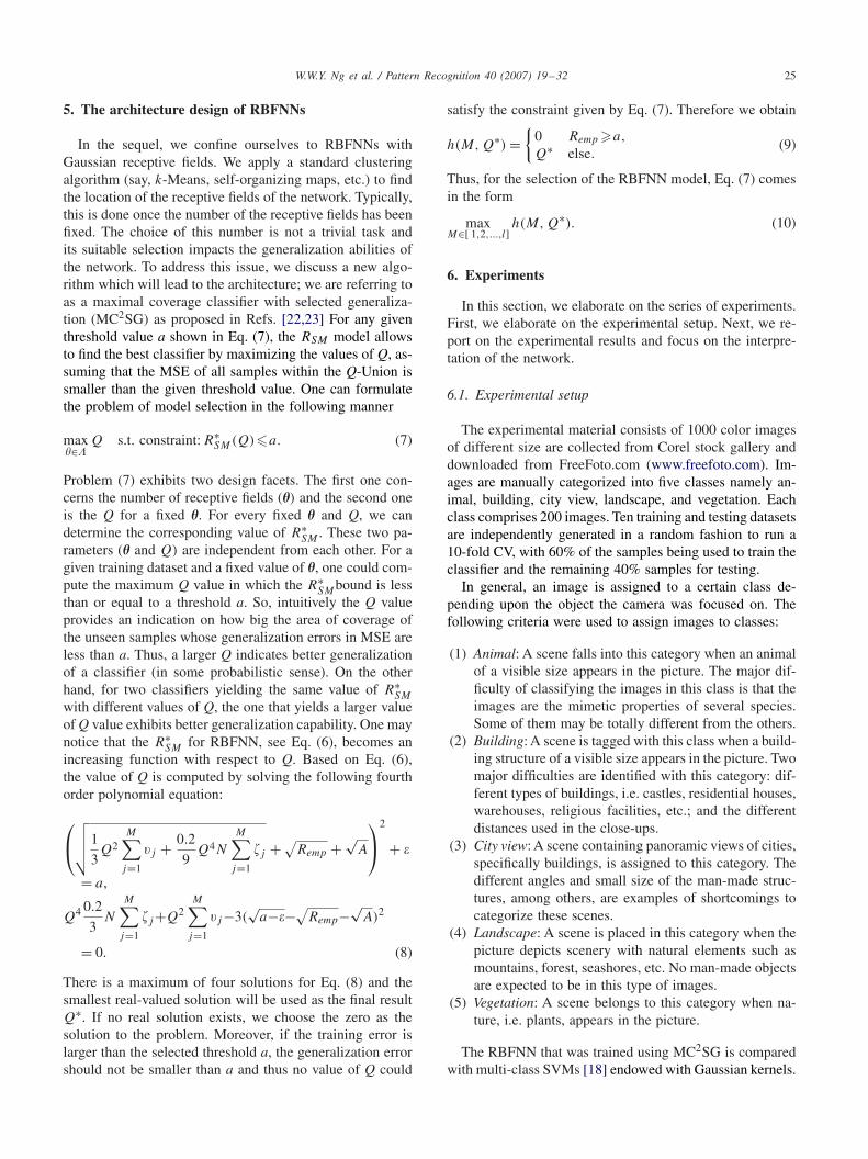
Fig. 3. Receptive fields against the number of images with highest acti-vation. Groups of nodes within the hidden layer resemble the semanticcategorization of data.

field represents the class of Buildings if the training imagethat is the closest to it is belongs to the Building class. Onemay observe that the number of receptive fields in classesAnimal, City View and Landscape are slightly larger thanthose for the classes of Building and Vegetation. This indi-cates that the varieties of these two categories representedin terms of color and texture descriptors are less diversi-fied than reported for the remaining three classes. For exam-ples, images that belong to the category of Buildings usuallyconsist of many vertical and horizontal edges. The color ofthe images belonging to the category Vegetation is predomi-nantly green. In contrast, images in the category of Animalsexhibit different shapes (edges and texture). The color alsoexhibits more diversity when more types of animals are in-volved in this class. On average, the numbers of receptivefields in all classes are nearly the same and this indicates thatthe complexity of recognizing image belonging to differentcategories could be equally challenging.

When using SVM, the images are projected to a very highdimensional kernel space and it is very difficult to visualizethe SVM or relate it to the problem domain knowledge.Instead, the RBFNN works in the original feature space inthe following section, we provide further analysis to theresulting RBFNN using the eighth training dataset, whichyields the highest testing accuracy among all.

For each image being fed to the RBFNN, one of the recep-tive fields yields the highest activation level. Fig. 3 shows thenumber of images yielding the highest activation for eachreceptive field. For example, the first receptive field comeswith 19 images in the Animal class yielding the highest ac-tivation but zero for other classes, therefore this receptivefield forms an abstraction for the Animal class. It offers aninsight into the relation between nodes in the hidden layer

Table 5Confusion matrix of RBFNN trained by MC2SG

63.80 ± 6.3 2.80 ± 1.7 3.20 ± 1.6 3.70 ± 1.8 7.30 ± 3.42.80 ± 2.0 65.90 ± 6.4 5.70 ± 2.1 3.70 ± 2.0 1.40 ± 0.84.20 ± 2.1 8.90 ± 3.2 57.60 ± 5.4 6.70 ± 2.6 0.30 ± 0.81.40 ± 0.9 0.50 ± 0.8 1.60 ± 1.2 75.60 ± 10.4 1.50 ± 0.96.30 ± 1.7 0.00 ± 0.0 1.00 ± 1.4 1.40 ± 1.3 72.70 ± 5.2

Table 6Confusion matrix of RBFNN trained by sequential learning

60.10 ± 5.4 3.70 ± 2.0 4.10 ± 1.5 4.80 ± 1.6 8.40 ± 3.13.60 ± 1.6 61.80 ± 7.2 8.00 ± 3.2 4.20 ± 2.2 2.00 ± 1.34.50 ± 1.8 9.60 ± 2.8 54.70 ± 5.7 8.40 ± 2.5 0.70 ± 0.91.90 ± 1.2 1.40 ± 1.0 2.10 ± 0.9 72.60 ± 10.5 2.10 ± 1.46.90 ± 2.1 0.80 ± 0.6 1.50 ± 1.4 2.60 ± 1.5 69.70 ± 4.9

Table 7Confusion matrix of SVM

54.90 ± 6.2 3.10 ± 1.2 5.10 ± 2.1 9.00 ± 2.6 8.70 ± 2.82.40 ± 0.8 55.30 ± 4.8 13.80 ± 1.7 6.30 ± 2.7 1.70 ± 1.03.70 ± 2.2 3.50 ± 2.0 59.50 ± 5.5 10.30 ± 2.6 0.70 ± 1.21.70 ± 1.0 1.10 ± 1.2 2.60 ± 1.1 74.10 ± 9.3 1.10 ± 1.19.60 ± 2.5 0.30 ± 0.4 0.40 ± 0.5 2.20 ± 1.6 68.90 ± 3.8

and the expected categorization of images produced by thenetwork.

Tables 5–7 present the average confusion matrices forthe testing dataset for RBFNN trained by MC2SG, RBFNNoptimized by sequential learning and SVM, respectively.RBFNN trained by MC2SG achieves higher accuracy than itscounterparts when classifying images belonging to classes:Animal, Building, Landscape, and Vegetation. The accuracyfor images ascribed to class City view is higher in compar-ison with RBFNN trained by sequential learning but lowerthan the one obtained by the SVM classifier. However, theconfusion between classes is lower in most of the cases whenusing RBFNN optimized by MC2SG than using the othertwo classifiers.

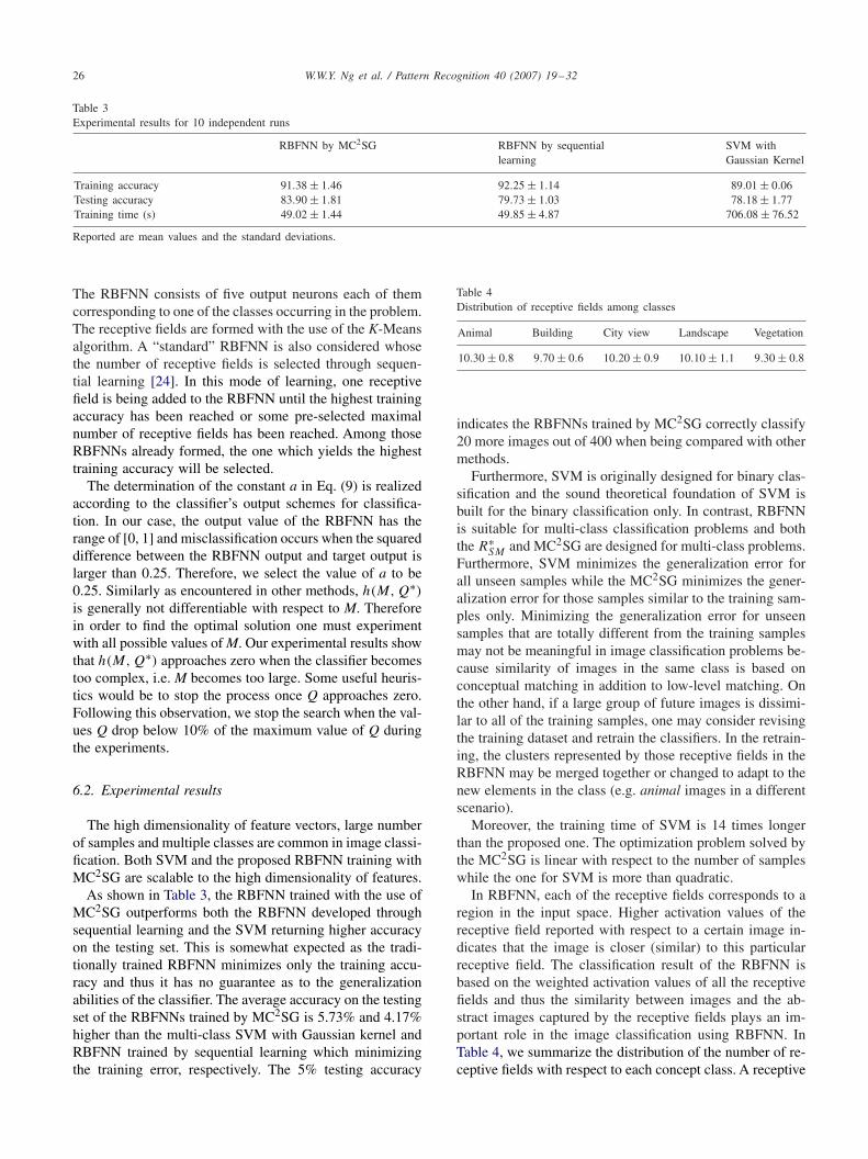
From the confusion matrices, one may notice that theclassifiers develop some confusion between the follow-ing pairs of classes: Animal&Vegetation, Building&Cityview, Building&Landscape, Landscape&City view andVegetation&Animal. These errors are somewhat anticipatedbecause of the commonalities of color and texture descrip-tions occurring in these classes. Furthermore, such possiblemisclassifications could be expected from the semanticpoint of view. For example, one can observe in Fig. 4 thatimages belonging to City view consist of many Buildingsand Animal images usually having the background simi-lar to Vegetation’s foreground. The pair of Landscape andCity view are similar in cases which the lower part of theimage is water while the upper part is either mountain orbuildings. It is also noted that animals exhibiting mimicryas the last four images depicted at the last row of Fig. 4 arefrequently misclassified as vegetation.

28 W.W.Y. Ng et al. / Pattern Recognition 40 (2007) 19–32

Fig. 4. Samples of expected misclassified images occurring due to semantic overlap.

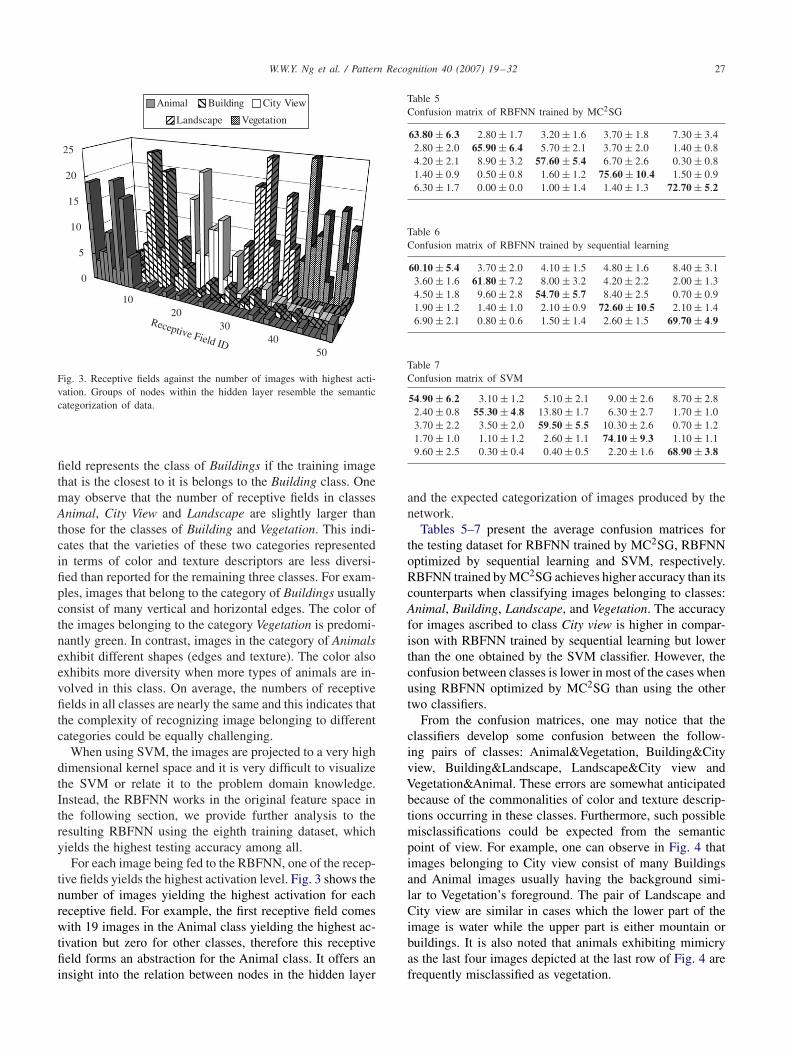
(a) (c) (e)(b) (d)

Fig. 5. Selected samples of misclassified images.

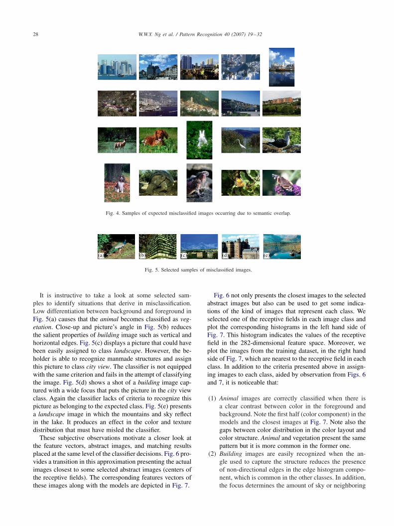
It is instructive to take a look at some selected sam-ples to identify situations that derive in misclassification.Low differentiation between background and foreground inFig. 5(a) causes that the animal becomes classified as veg-etation. Close-up and picture’s angle in Fig. 5(b) reducesthe salient properties of building image such as vertical andhorizontal edges. Fig. 5(c) displays a picture that could havebeen easily assigned to class landscape. However, the be-holder is able to recognize manmade structures and assignthis picture to class city view. The classifier is not equippedwith the same criterion and fails in the attempt of classifyingthe image. Fig. 5(d) shows a shot of a building image cap-tured with a wide focus that puts the picture in the city viewclass. Again the classifier lacks of criteria to recognize thispicture as belonging to the expected class. Fig. 5(e) presentsa landscape image in which the mountains and sky reflectin the lake. It produces an effect in the color and texturedistribution that must have misled the classifier.

These subjective observations motivate a closer look atthe feature vectors, abstract images, and matching resultsplaced at the same level of the classifier decisions. Fig. 6 pro-vides a transition in this approximation presenting the actualimages closest to some selected abstract images (centers ofthe receptive fields). The corresponding features vectors ofthese images along with the models are depicted in Fig. 7.

Fig. 6 not only presents the closest images to the selectedabstract images but also can be used to get some indica-tions of the kind of images that represent each class. Weselected one of the receptive fields in each image class andplot the corresponding histograms in the left hand side ofFig. 7. This histogram indicates the values of the receptivefield in the 282-dimensional feature space. Moreover, weplot the images from the training dataset, in the right handside of Fig. 7, which are nearest to the receptive field in eachclass. In addition to the criteria presented above in assign-ing images to each class, aided by observation from Figs. 6and 7, it is noticeable that:

(1) Animal images are correctly classified when there isa clear contrast between color in the foreground andbackground. Note the first half (color component) in themodels and the closest images at Fig. 7. Note also thegaps between color distribution in the color layout andcolor structure. Animal and vegetation present the samepattern but it is more common in the former one.

(2) Building images are easily recognized when the an-gle used to capture the structure reduces the presenceof non-directional edges in the edge histogram compo-nent, which is common in the other classes. In addition,the focus determines the amount of sky or neighboring

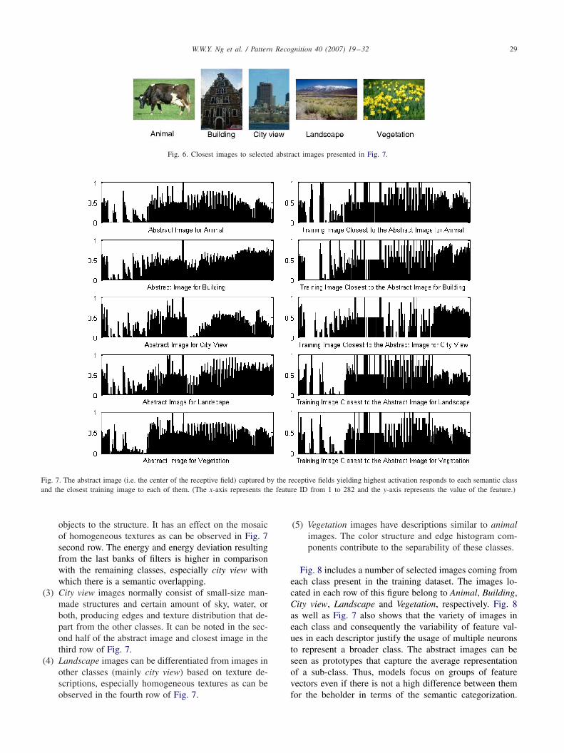
W.W.Y. Ng et al. / Pattern Recognition 40 (2007) 19–32 29

Fig. 6. Closest images to selected abstract images presented in Fig. 7.

Fig. 7. The abstract image (i.e. the center of the receptive field) captured by the receptive fields yielding highest activation responds to each semantic classand the closest training image to each of them. (The x-axis represents the feature ID from 1 to 282 and the y-axis represents the value of the feature.)

objects to the structure. It has an effect on the mosaicof homogeneous textures as can be observed in Fig. 7second row. The energy and energy deviation resultingfrom the last banks of filters is higher in comparisonwith the remaining classes, especially city view withwhich there is a semantic overlapping.

(3) City view images normally consist of small-size man-made structures and certain amount of sky, water, orboth, producing edges and texture distribution that de-part from the other classes. It can be noted in the sec-ond half of the abstract image and closest image in thethird row of Fig. 7.

(4) Landscape images can be differentiated from images inother classes (mainly city view) based on texture de-scriptions, especially homogeneous textures as can beobserved in the fourth row of Fig. 7.

(5) Vegetation images have descriptions similar to animalimages. The color structure and edge histogram com-ponents contribute to the separability of these classes.

Fig. 8 includes a number of selected images coming fromeach class present in the training dataset. The images lo-cated in each row of this figure belong to Animal, Building,City view, Landscape and Vegetation, respectively. Fig. 8as well as Fig. 7 also shows that the variety of images ineach class and consequently the variability of feature val-ues in each descriptor justify the usage of multiple neuronsto represent a broader class. The abstract images can beseen as prototypes that capture the average representationof a sub-class. Thus, models focus on groups of featurevectors even if there is not a high difference between themfor the beholder in terms of the semantic categorization.

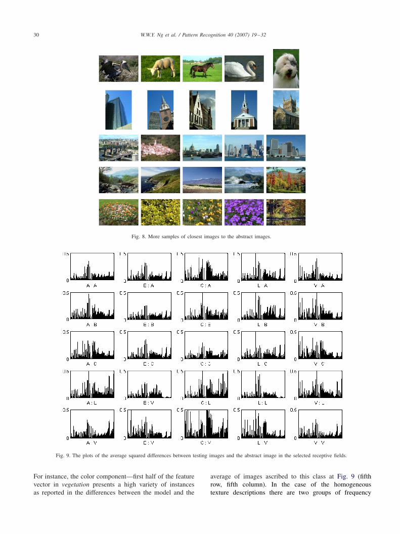
30 W.W.Y. Ng et al. / Pattern Recognition 40 (2007) 19–32

Fig. 8. More samples of closest images to the abstract images.

Fig. 9. The plots of the average squared differences between testing images and the abstract image in the selected receptive fields.

For instance, the color component—first half of the featurevector in vegetation presents a high variety of instancesas reported in the differences between the model and the

average of images ascribed to this class at Fig. 9 (fifthrow, fifth column). In the case of the homogeneoustexture descriptions there are two groups of frequency

W.W.Y. Ng et al. / Pattern Recognition 40 (2007) 19–32 31

filters. One may notice that the values of the low frequencyfilters yielding a very high variance produces high dif-ferences between the images and abstract images of theirclasses (diagonal form left to right in Fig. 9). The exceptionis class landscape (fourth row, fourth column), which asmentioned above, relies on this descriptor to discriminatefrom other classes.

In Fig. 9, we use the notation of “A:B” to denote theplot of the average differences between the abstract imageof animal and testing samples of building. (A: Animal, B:Building, C: City view, L: Landscape and V: Vegetation.)Columns correspond to the model, while rows refer to thetesting sample. The diagonal shows the highest matching.

Finally, it is worth to stress the contribution of the lo-calized generalization error model in selecting the RBFNNarchitecture that produces significant separability and dis-crimination between classes, though the description of im-ages does not capture enough criteria to resemble semanticcharacterization of these classes.

7. Conclusions

In this study, being motivated by the concept that se-mantically similar images should exhibit similarity in thefeature space, we proposed an application of the localizedgeneralization error model to image classification. Thismodel captures the generalization error for unseen samplesthat are similar to the training samples. Experimental re-sults show that the RBFNN trained using the minimizationof the localized generalization error outperforms “standard”RBFNN and multi-class SVM. Moreover, we showed howthe RBFNN could be helpful in the visualization of thereceptive fields with respect to the categories of images tobe classified.

The selection of the MPEG-7 descriptors (the featurespace) for describing images is still an open problem. In thiswork, we formed the MPEG-7 feature space to describe im-ages by balancing the number of color and texture descrip-tors. However, further detailed investigations on the forma-tion of the optimal feature space become necessary. It is verylikely that some classes of images may be distinguished wellby some MPEG-7 descriptors however the choice of suchdescriptors could depend upon the character of the classes.While here we decided to consider 5 predefined categoriesof images, one should become aware that more work is nec-essary to fully explore the capabilities of the MPEG-7 de-scriptors as a basis of the most suitable feature space. Oneinteresting alternatives would be to form the feature spacewith the aid of the localized generalization error model.

Acknowledgments

This work is supported by a Hong Kong Polytechnic Uni-versity Interfaculty Research Grant No. G-T891 and CanadaResearch Chair (W. Pedrycz).

References

[1] T. Hastie, R. Tibshirani, J. Friedman, The Element of StatisticalLearning, Springer, New York, 2001.

[2] V. Vapnik, Statistical Learning Theory, Wiley, New York, 1998.[3] V. Cherkassky, X. Shao, F.M. Mulier, V.N. Vapnik, Model complexity

control for regression using VC generalization bounds, IEEE Trans.Neural Networks 10 (5) (1999) 1075–1089.

[4] B.S. Manjunath, P. Salembier, T. Sikora, Introduction to MPEG-7Multimedia Content Description Interface, Wiley, New York, 2002.

[5] E. Izquierdo, I. Damnjanovic, P. Villegas, X. Li-Qun, S. Herrmann,Bringing user satisfaction to media access: the 1st busman project,IEEE Proceedings of the International Conference on InformationVisualisation, 2004, pp. 444–449.

[6] V. Mezaris, H. Doulaverakis, R.M.B. de Otalora, S. Herrmann, I.Kompatsiaris, M.G. Strintzis, A test-bed for region-based imageretrieval using multiple segmentation algorithms and the MPEG-7 experimentation model: the schema reference system, Imageand Video Retrieval, Lecture Notes in Computer Science, 2004,pp. 592–600.

[7] S.-F. Chang, T. Sikora, A. Puri, Overview of the MPEG-7 standard,IEEE Trans. Circuits Systems Video Technol. 11 (6) (2001) 688–695.

[8] A. Dorado, W. Pedrycz, E. Izquierdo, An MPEG-7 learning space forsemantic image classification, Proceedings of the 31st Latin AmericanComputing Conference, Cali, Colombia, 2005, pp. 297–307.

[9] B.S. Manjunath, J.-R. Ohm, V.V. Vasudevan, A. Yamada, Color andtexture descriptors, IEEE Trans. Circuits Systems Video Technol. 11(6) (2001) 703–715.

[10] A. Barla, F. Odone, A. Verri, Old fashioned state-of-the-art imageclassification, IEEE Proceedings of International Conference onImage Analysis and Processing, 2003, pp. 566–571.

[11] A.K. Jain, P.W. Duin, J. Mao, Statistical pattern recognition: a review,IEEE Trans. Pattern Anal. Mach. Intell. 22 (1) (2000) 4–37.

[12] O. Chapelle, P. Haffner, V.N. Vapnik, Support vector machines forhistogram-based image classification, IEEE Trans. Neural Networks10 (5) (1999) 1055–1064.

[13] N. Serrano, A. Savakis, A. Luo, A computationally efficientapproach to indoor/outdoor scene classification, IEEE Proceedings ofInternational Conference on Pattern Recognition, 2002, pp. 146–149.

[14] R. Yan, Y. Liu, R. Jin, A. Hauptmann, On predicting rare classeswith SVM ensembles in scene classification, IEEE Proceedingsof International Conference on Acoustics, Speech, and SignalProcessing, 2003, pp. 21–24.

[15] C.-F. Tsai, K. McGarry, J. Tait, Image classification usinghybrid neural networks, ACM SIGIR Proceedings of InternationalConference on Research and Development in Information Retrieval,2003, pp. 431–432.

[16] S. Prabhakar, H. Cheng, J.C. Handley, Z. Fan, Y.W. Lin,Picture–graphics color image classification, IEEE Proceedings ofInternational Conference on Image Processing, 2002, pp. 785–788.

[17] S.-B. Dong, Y.-M. Yang, Hierarchical web image classification bymulti-level features, in: Proceedings of International Conference onMachine Learning and Cybernetics, Beijing, China, November 2002,pp. 663–668.

[18] K. Crammer, Y. Singer, On the algorithmic implementation ofmulticlass Kernel-based vector machines, J. Mach. Learn. Res. 2 (2)(2002) 265–292.

[19] Y. Cheng, J. Lu, T. Yahagi, Car license plate recognition based onthe combination of principal components analysis and radial basisfunction networks, IEEE Proceedings of International Conference onSignal Processing, 2004, pp. 1455–1458.

[20] Y. Fan, M. Paindavoine, Implementation of an RBF NeuralNetwork on embedded systems: real-time face tracking and identityverification, IEEE Trans. Neural Networks 14 (5) (2003) 1162–1175.

[21] W. Hoeffding, Probability inequalities for sums of bounded randomvariables, J. Am. Stat. Assoc. 58 (1963) 13–30.

32 W.W.Y. Ng et al. / Pattern Recognition 40 (2007) 19–32

[22] W.W.Y. Ng, D.S. Yeung, D. Wang, E.C.C. Tsang, X.-Z.Wang, Localized generalization error and its application toRBFNN training, in: Proceedings of International Conference onMachine Learning and Cybernetics, Guangzhou, China, 2005,pp. 4667–4673.

[23] D.S. Yeung, W.W.Y. Ng, D. Wang, E.C.C. Tsang, X.-Z. Wang,Localized generalization error model and its application to

architecture selection for radial basis function neural network, IEEETrans. Neural Networks, submitted for publication, second review.

[24] L. Yingwei, N. Sundararajan, P. Saratchandran, A sequential learningscheme for function approximation using minimal radial basisfunction neural networks, Neural Comput. 9 (1997) 461–478.